IIIIIIIIIIIII\1

-III(I

I

ESTIMATING ONE MEAN OF A BIVARIATE NORMAL DISTRIBUTIONUSING A PRELIMINARY TEST OF SIGNIFICANCE AND A TWO STAGE

SAMPLING SCHEME

By

D. R. Brogan and J. Sedransk

Department of Biostatistics, U. N. Cand

Department of Statistics, University of Wisconsin

Institute of Statistics Mimeo Series No. 752

June 1971

II

(IIIIIIIIIIIIIIIII

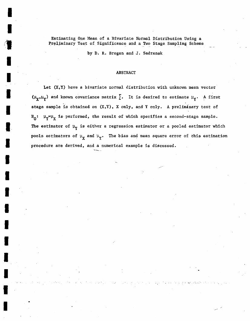
Estimating One Mean of a Bivariate Normal Distribution Using aPreliminary Test of Significance and a Two Stage Sampling Scheme

by D. R. Brogan and J. Sedransk

ABSTRACT

Let (X,Y) have a bivariate normal distribution with unknown mean vector

(llx, l1y) and known covariance matrix r. It is desired to estimate ].ly' ·A first

stage sample is obtained on (X,Y), X only, and Y only. A preliminary test of

HO: lly=llx is performed, the result of which specifies a second-stage sample.

The estimator of l1y is either a regression estimator or a pooled estimator which

pools estimators of ].lX and lly' The bias and mean square error of this estimation

procedure are derived, and a numerical example is discussed.-_._~

..-

by D. R. Brogan and J. Sedransk*

Let the random variable (X,Y)' follow the bivariate normal distribution

(1.l)

After this preliminary test, a second~;&PX is tested.native hypothesis H1 :

1. Statement of the Problem and Examples

It is desired to estimate Py when there is evidence that perhaps Py=PX• There

are available n>O bivariate-observations on (X,Y), an additional n~>O inde­

pendent observations on X, and an additional ny>O independent observations on

Y: Using these observations, the null hypothesis HO

: Py=PX versus the a1ter-

Estimating One Mean of a Bivariate Normal Distribution Using aPreliminary Test ,of Significance and a Two Stage Sampling Scheme

with mean vector E{X,Y), = (pX,~)f and known covariance matrix L, where

stage of sampling is carried out on one, two or three of the following random, ,,-

*D. R. Brogan is Assistant Professor, Department of Biostatistics, Universityof North Carolina School of Public Health. J. Sedransk is Associate Professor,Department of Statistics, University of Wisconsin. This research was partiallysupported by National Institutes of Health Biometry Training Grant 5TlGM34,National Institute of Mental Health Training Grant MH10373, and National Centerfor Educational Statistics (U.S. Office of Education) Contract Number OEC-3­002041-2041.

variables: (X,Y) only, X only, and Y only. The estimator of Py , using data

from the first and second stages of sampling, depends upon the acceptance or

rejection of HO• This general estimator reduces in special cases to estimators

proposed by other authors who have considered the "preliminary test" approach to

II)Ii

II,IIIIIIIIIIII'II

II

~'I

IIIIIIIIIIIIIIII

-2-

estimating ~Y' In this paper, the bias and mean square error of the proposed

estimator are derived.

A situation where such an estimation scheme would be appropriate is the

estimation of the average systolic blood pressure (SBP) of a hospital population.

SBP is available on each admitted patient's hospital record. However, it is

well known that SBP varies within each person depending upon time of day,

general level of excitement, and so on. Hence, theoretically, measurements of

SBP should be" taken on a random sample of admitted patients und~r some set of

standard conditions. Then, one could easily estimate ~Y' where Y is SBP measured

under the set of st~ndard conditions. However, since measurements on Yare

difficult (and expensive) to obtain, it would be hoped that measurements on X,

SBP measured under non-standard conditions, for a relatively large sample of

patients might be used in conjunction with measurements on Y for a relatively

small sample of patients in order to estimate ~Y' In this example, it may be

that 1~-~xl is small; almost certainly, though, a~ would be larger than a;.A random sample on X at the first stage could be collected from past

hospital records where, it is assumed, SBP was measured under non-standard con­

ditions. An independent bivariate random sample on (X,Y) could be obtained by

measuring SBP under standard conditions on a sample of patients, as well as by;r

using the usual SBP from the hospital records of the same patients. A further,

independent, random sample on Y at the first stage (though not necessary) could

possibly come from a research project done on some of the hospital population

where SBP was purposely taken under standard conditions and the SBP under non-

standard conditions is not available. Of course, it is necessary to take

caution that these three samples do, indeed, come from the same population.

F~ther sampling can be done at the second stage under several options (see~. ~ . . - .

II'IIIIIIIIIIIIIIIII

-3-

Section 3).

Letting CX' CY' and Cxy be the respective per unit costs of measuring SBP

under non-standard, standard, and both conditions, it is obvious in this example

that Cx<Cy<Cxy.<Cx+Cy • Hence, observations on X may be "preferred to",pbserva­

tions on Y if X can be used effectively to estimate ~Y. This type of cost con­

figuration is typical of many situations in which one might wish to apply the

preliminary test approach discussed in this paper. That is, one wishes. to

estimate ~y' but an observation on X is less costly than an obs~vation on Y

and there is some p~ior evidence that ~y=~X.

Another example is that of estimating the average volume of trees in a

forest. For any given tree it is possible to measure Y, the actual volUme. This,

however, is difficult and expensive. A much cheaper method which may provide a

good estimate of the volume is to measure the height H of the tree and' the dia­

meter D at a specified height off the ground. Then the volume is estimated by

X = kD2H. If 1~-~xl is small, then measureme~ts of X could be pooled with

measurements of Y in order to estimate ~.

Still another example is the post-enumeration surveys which~the Census

Bureau conducts to check on the adequacy of coverage and content in the decennial

census of population,and housing [Bailar, 8]. For each of several geographic;r

areas, there could be available the population count or the attribute data from

the post-enumeration survey (i.e. Y) and from the original census (i.e. X).

These observations can possibly be combined in order to estimate the total pop­

ulation or the average value of some attribute for these areas. It would be

hoped that the combined estimate would be more accurate than the census figures

alone.

II~I

II.IIIIIIIIIIIIII

• t

-4-

These three examples illustrate the following considerations: (1) a pooled

estimator seems appropriate if I~Y-~Xr is small; (2) observations on X instead

of Yare desirable from a cost viewpoint; and (3) a correlation between X and Y

may allow utilization of information on X even though l~y-~xl is not small.

2. Previous Investigations of Related Problems

Some of the authors who have studied parametric estimation problems by

using pooling. procedures after a preliminary test of significance are Mosteller4

[17], Bennett [10, 11], Kitagawa [15], Bancroft [9], Asano. [3, 4; 5], Kale and

Bancroft [14], Han and Bancroft [12], Asano and Sugimura [7], and Huntsberger

[13]. Asano and Sato [6] and Sato [19] have considered two bivariate populations

and two multivariate populations, respectively. Tamura [20, 21] has considered

non-parametric estimation after a preliminary test of significance.

This study differs from these other investigations in three respects.

First, there is no published research where a two-stage sampling procedure has

been considered in conjunction with a preliminary test of significance. The,/

two-stage estimation procedures discussed, for example, by Yen [22] and Arnold- .r_

and Al-Bayyati [2], use information from the first stage to determine the

sampling plan at the second stage, but a preliminary tes.t of significance is

not used to make this determination. The two-stage sampling scheme is useful

because, for a given budget (assuming CX<Cy~Cxy)' it may be advantageous to do

some additional sampling after the preliminary test is done. For example, if

HO

: ~=~X is accepted, then a large sample where only X is measured is reason­

able for the second stage. However if HO: ~Y=~X is rejected, then a small

sample where only Y is measured is probably more feasible for the second stage.

In addition, the method proposed here allows a bivariate sample on (X,Y) at the

second stage.

II

0"

IIIIIIIIIIIIIIII

-5-

Second, there are no published results where both independent and dependent

sampling can be included atueach stage. Thus,·given a budget and cost function,

in the procedure proposed here one can, at least theoretically, determine the

optimal allocation of resources (1) between sampling at the first and second

stages, and (2) among bivariate and univariate (both X and Y) sampling at each

stage.

Third, every investigator except Kitagawa [15] and Mehta and Gurla!1d [16]..

has considered the random variables X and Y to be independent. Mehta and

Gurland [16]"however, are concerned with testing hypotheses about a bivariate

normal population, Qne of which is the null hypothesis that p=O. Kitagawa [15],

on the other hand, considers p#O, where p is unknown, although his investigation

is speci~lized by having only a one-stage bivariate sample of size n with----

cr~=cr~=cr2 •

In many prospective applications of the preliminary test approach (such

as the SBP example) it is to be expected that cr~#cr~. Further, it is important

to extend the results available for "pooling means" to include the numerous

applications where p is not necessarily zero, and where random samples of sizes

n>O, ~>O, and ny>O as described in Section 1 are selected. Thus, to avoid

having to. us.e approx~mate distribution theory, I has be~n assumed to be known;r

in this investigation. A small Monte Carlo study has been carried out to deter-

mine the effect on the bias and mean square error of the estimator of ~Y from

estimating the components of I [Ruhl, 18].

Finally, it may also be noted that (1) those authors considering cr~#cr~

[e.g. 10] assume that cr~ and cr~ are known; and (2) some of the authors [14, 17]

-6-

.---

are the same as those studied by many of the above authors except for those

3. The Sampling Procedure, Some Notation, and Some Special Cases

Y be the sample means from the two inde-nyAnalogously, if HO is accepted, let the

A random sample (Xl,Yl), ••• ,(Xn,Yn) is selected from the bivar~at~ normal

distribution.. In addition, an independent random sample of nX ~bservations is4

taken on X, and a random sample of ny obs~rvations is taken on Y~ In the first

stage sample, thus, are (n~) observations on X and (n+ny) observations on Y.

Note that only Xi and Yi are correlated, (i=l, ••• ,n), where (Xi,Yi ) denotes

the i-th element in the. bivariate sample.

who take cr~=cr~=cr2 assume, for simplicity, that cr2 is known.

Special cases of the sampling procedure considered in this investigation

investigations where cr2=cr2=cr2 and/or p are assumed to be unknown.X Y

At this point a preliminary test of the null hypothesis HO: ~=~X versus

the alternative hypothesis HI: ~y:;'J.1x is done using the sample data from the

first stage. On the basis of the preliminary test HO is either accepted or

rejected. A second stage sample is then taken, again allowing a bivariate sample

on (X,Y) and two independent samples, one each on X and Y. If H9

_is accepted,

the size of the bivariate sample will be nO' and the size of the independent

samples on X and Y will be nOX and nOY' respectively. ~imilarly, if HO is

•rejected, the sizes of the samples at the second stage will be nl , nIX' and nly •

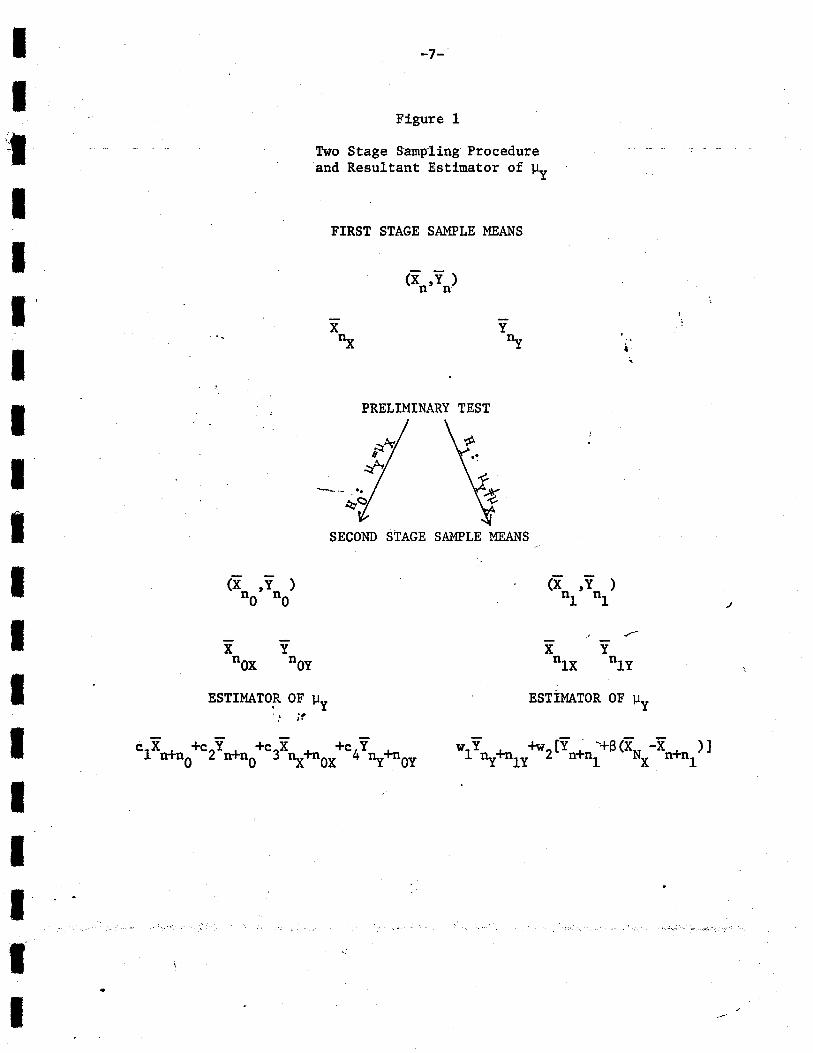
Thus, the notation for this sampling procedure can be summarized as follows.

Let X and Y be the sample means on X and Y from the bivariate sample at then n _

first stage. Likewise, let X and~

pendent samples at the first stage.

respective sample means be denoted byX , Y ,X ,and Y • If H~ is rejected,nO nO nOX nOY v

the sample means will be X , Y , X ,and Y • The notation and sampling_ _ n1 n1 . nlX n1yscheme are illustrated in Figure 1.

IIIIIIIIIIII

II

-'IIIII

----_._-_.--- .---

ESTiMATOR OF lly

(x tY )n n

-7-

Figure 1

PRELIMINARY TEST

x~

FIRST STAGE SAMPLE MEANS

--

Two Stage Sampling Procedureand Resultant Estimator of ~Y

" jf

ESTIMATO;a OF lly

SECOND STAGE SAMPLE MEANS

\ '

c1x +n +c2Y + +c3X +n +c4Y +nnOn nO ~ OX ny OY

II

1\1

IIIIIIIIIIIIII-II

-8-

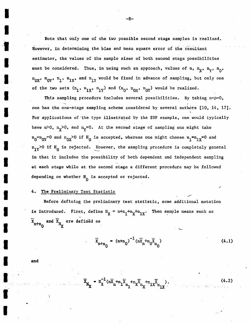
estimator, the values of the sample sizes of both second stage possibilities

Before defining the preliminary test statistic, some additional notation

(4.1)

(4.2)

However, the sampling procedure is completely general---~ -

-1 - - - -K..y = NX (nX +nIX -ML_X +nUX ) •Jo'x. n n1 --x: ~ . nlX .

However, in determining the bias and mean square error of the resultant

Note that only one of the two possible second stage samples is realized.

must be considered. Thus, in using such an approach, values of n, ~, ny, nO'

nOX' nOY' nl , nIX' and nly would be fixed in advance of sampling, but only one

of the two sets (nl , nIX' nly) and (nO' nOX ' nOY) would be realized.

This sampling procedure includes several possibilities. By takin~ n=p=O,

one has the one-stage sampling scheme considered by several authOrs [10, 14, 17].

For applications of 'the type il1ustra~ed oy the SBP example, one would typically

have n>O, nx>O, and ~=O. At the second stage of sampling one might take

nO=nOY=O and nOX>O if HO is accepted, whereas one might choose n1=n1X=0 and

nly>O if HO is rejected.

at each stage while at the second stage a different procedure may be followed

in that it includes the possibility of both dependent and independent sampling

depending on whether HO

is accepted or rejected.

4. The Preliminary Test Statistic

is introduced. First, define NX = n+nl +nX+n1X' Then sample means such as

X +n and ~are defined asn 0 X

and

II~I

II.IIIIIIIIIIIII'I

-9-

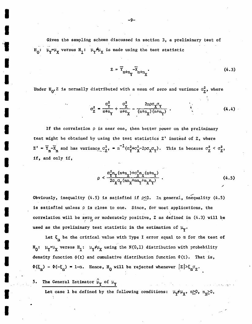
Given the sampling scheme discussed in section 3, a preliminary test of

(4.3)

(4.4)

(4.5)

This is because cr2 < cr2Z Z'

.,,-Obviously, inequality (4.5) is satisfied if p<O. In general, inequality (4.5)

If the correlation p is near one, then better power on the preliminary

test might be obtained by using the test statistics Z' instead of Z, where

Under HO'Z is normally distributed with a mean of zero and variance cr~, where

HO: Py=~X versus Hl : ~Y~X is made using the test statistic

Z' = Yn-Xn and has varianC~_?~,

if, and only if,

is satisfied unless p is close to one. Since, for most applications, the

correlation will be zero or moderately positive, Z as defined in (4.3) will be.' if

used as the preliminary test statistic in the estimation of ~.

Let ~a be the critical value with Type I error equal to a for the test of

HO: Py=~X versus Hl : ~Y~~X using the N(O,l) distribution with probability

density function ~(t) and cumulative distribution function ~(t). That is,

~(~a) - ~(-~a) = l-a. Hence, HO will be rejected whenever Izl>~acrz·

"5. The General Estimator ~Y of ~Y

Let case 1 be defined by the following conditions: Py~~X' n>O, nx~O,

II'~I

IIIIIIIIIIIIII-II

-10-

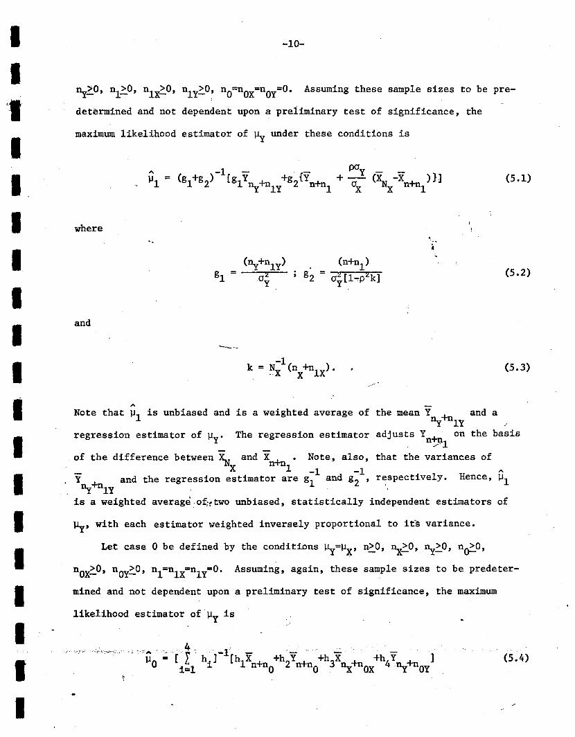
(5.2)

(5.3)

(5.1)

(5.4)

the mean Y +n and atty 1Y "

adjusts Yn+n on the basis. /1

that the variances of

(n+n1)

g2 =cr~[1...,p2k]

The regression estimator

---

where

ny,>0, n1>0, n1~>0, n1Y~0, nO=nOX=nOY=O. Assuming these sample sizes to be pre­

determined and not dependent upon a preliminary test of significance, the

maximum likelihood estimator of ~Y under these conditions is

and

A

Note that ~1 is unbiased and is a weighted average of

~, with each estimator weighted inversely proportional to its variance.

of the difference between XN and X +n. Note, also,X n 1 -1 -1 A

Y +n and the regression estimator are gl and g2 ' respectively. Hence, ~1

tty 1Y .is a weighted average:o~~two unbiased, statistically independent estimators of

regression estimator of ~y.

Let case 0 be defined by the conditions ~=~X' n>O, ~>O, Uy>O, n~O,

nOX>O, nOY>O, n1=n1X=n1Y=0. Assuming, again, these sample sizes to be predeter­

mined and not dependent upon a preliminary test of significance, the maximum

likelihood estimator of'~y is

II~I

IIIIIIIIIIIIIIfI

/

-11-

to be an arbitrary known constant.

(5.7)

(5.6)

where

hI(n+n

O)

[l. - ~]. h3

= (~+nox)/a~= (l_pZ) a2 a a 'X X Y(5.5)

h2 =(n+no) [5- - ~]. h4 (ny+nOY ) I a~ •(l_pZ) (J a a ' =

y X Y

A-

Note that ~O is a weighted average of four unbiased estimators of ~ and hence

unbiased. The weights hi' i=1, ••• ,4, as defined in (5.5), minimize the variance

These two maximum likelihood estimators suggest the definition of the

A- A-

accepted, then the estimator ~ of ~y is defined as ~YO where--._-

A-

of ~O.

estimator of ~ under the possibilities of accepting or rejecting HO• If HO is

A- A-

If HO is rejected, then the estimator ~y of ~y is defined as ~Yl where

4Reasonable choices for wi and ci would be wi = gi/ (gl+g2) and ci = hi/[ r hi]·

. i=1Likewise, a reasonable choice for a would be pay/aX as suggested by (5.1).

However, these choices will not necessarily minimize the variance or mean square

A-

For the derivation of the bias and mean square error of~~y' wi' i=1,2, and

ci ' i=1,2,3,4, are assumed to be arbitrary known constants such that (5.6) and

(5.7) are satisfied. Also, the regression coefficient a in (5.7) is assumed

II(I

IIIIIIIIIIIIIIII

-12-

as

where all terms have been previously defined in (4.3), (4.4), (5.6), and (5.7) •

(6.2)

(6.3)

(6.4)

I -2;t(A Z=z) = ~A+crz (z-~)Cov(A,Z).

"The expectation of ~y is defined as

If now A and Z are bivariate normal random variables, where A has uncon-~

E(~) = E[~Ylllzl>~a(Jz]pr[/zl>~a(Jz] + E[~ollzl<~a(Jz]pr[/.~I<~a(J~'] (6.1)

•

"error of lly even though they do minimize the variance of the maximumlik~lihood

"estimators from which ~ was defined. Hence, for generality, the bias and mean

square error are derived for wi' ci ' and 13 being known constants.

"6. Bias of ~

.-This can be written as

mean ~ = ~-~X and variance (J~ as defined in (4.4).

where h(z) is the density function of Z, and z- is normally distributed with

ditional expectation ~A' Anderson [1] shows that

A

Using (6.3) to obtain the conditional expectations in (6.2), E(~y) is obtained

II,IIIIIIIIIIIIII'fI

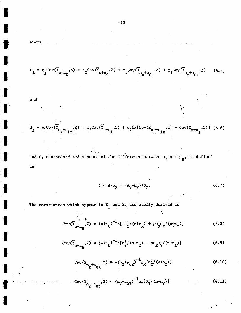
(6.10)

·(6.11)

(6.8)

(6.9)

.(6.7)

Cov(Y +n ,Z)I1y OY

'.'- ;f

Cov(Xn+n ,Z)o

--._-

-13-

/

where

HI = c Cov(X + ,Z) + c2cov(Yn+n0

'Z) + c3Cov(X +n ,Z) + c4Cov(Y +n ,Z) (6.5)1 n nO nX OX Ily OY

and

and 0, a standardized measure of the difference between ~ and ~x' is defined

as

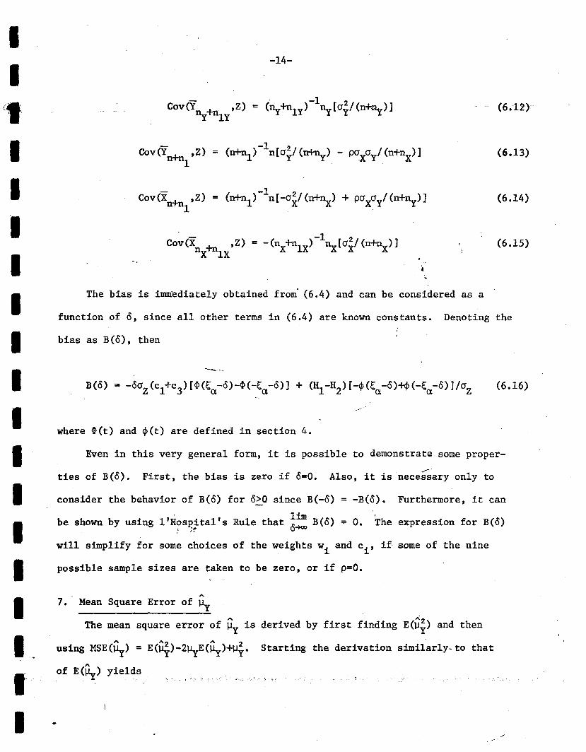
The covariances which appear in HI and H2 are easily derived as

IIII,

IIIIIIIIIIIIII'II

(6;12)

(6.16)

(6.15)

(6.14)

(6.13)

~

Also, it is necessary only to

Starting the derivation similarly. to that

Cov(X +n ,Z)nX IX

First, the bias is zero if 0=0.

Cov(Yn+n ,Z)1

The bias is immediately obtained from" (6.4) and can be considered as a

ties of B(o).

Even in this very general form, it is possible to demonstrate some proper-

---.-.

function of 0, since all other terms in (6.4) are known constants. Denoting the

-14-

bias as B(o), then

where ~(t) and ~(t) are defined in section 4.

consider the behavior of B(o) for 0>0 since B(-o) = -B(o). Furthermore, it can

" limbe shown by using l'H?s~!ta1's Rule that o~ B(o) = O. The expression for B(o)

" --

,.,7. Mean Square Error of ~

The mean square error of ~Y is derived by first finding E(a~) and then

will simplify for some choices of the weights wi and ci ' if some of the nine

possible sample sizes are taken to be zero, or if p=O.

,.,using MSE(~) =

,.,of E(~) yields

II('~

II"IIIIIIIIIIIIII

jf

and

(7.1)

(7.2)

(7.5)

(7.4)

-15-

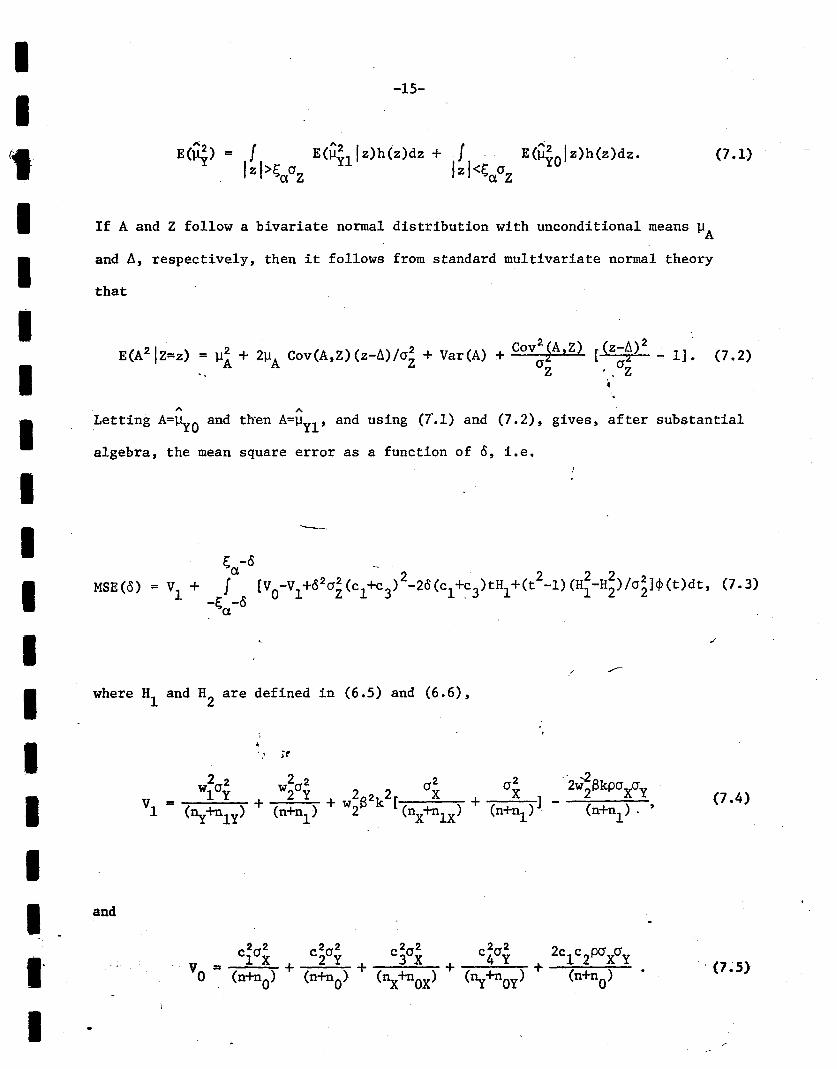
E{~) =

(A21 ) 2 2 C (A Z)( A)/ 2 + V (A) + Cov2

(A,Z) [(Z-fr)2 -,1].'E Z=z = ~A + ~A ov, Z-u crz ar 2crz .. crz..

---.

that

If A and Z follow a bivariate normal distribution with unconditional means ~A

and A, respectively, then it follows from standard multivariate normal theory

E; -0

MSE(o) = VI + _~J:o [VO-vl+02a~(cI+C3)2_20(cI+C3)tHI+(t2_1)(H~-H~)la~1~(t)dt. (7.3)

a

'" '"Letting A=~O and then A=~Yl' and using (1.1) and (7.2), gives, after substantial

algebra, the mean square error as a function of 0, i.e.

where HI and H2

are defined in (6.5) and (6.6),

IIttIIIIIIIIIIIIIII'I

II'I:IIIIIIIIIIIIII,I

-16-

A A.

Note that Vo and VI are the unconditional. variances of ~yo and ~Yl' respectively. -

A few properties of MSE(o) can be ascertained in this general form. First,

mean square error is a symmetric function of 0, i.e. MSE(-o) = MSE(o). Hence,

it is necessary only to investigate the behavior of MSE(o) for o~o. Second,

it can be shown that ~~ MSE(o) = VI' the unconditional variance of ~Yl. Third,

MSE(O) is equal to the unconditional variance of ~Yl' i.e. VI' plus another term

which can either be positive or negative.

The expression for MSE(o) in (7.3) can be integrated and written as in (6.16)

as a function of ¢(x) and ~(x), where x takes the value (~ -0) or (-~ -0). Onea a

of us has written a computer program to evaluate the bias and mean square error

as given in equations (7.3) and (6.16). What is typically done in studies of

preliminary test procedures is to evaluate the bias and mean square error for-..- --.

various values of a and ~ or 0, for some given sample sizes and variance-covariance

matrix. This paper presents the additional problem, however, of determining

values for the weights wi and ci and the regression coefficient B.

8. Choice of the Weights w. and c. and the Regression Coefficient B1 1 ~

It is theoretically possible to choose the w., c., and B so that the mean square1 1

error as given in (7.3) is minimized. If this is pursu~d, however, three things

become evident. First,;~he solution for wI' w2 ' and B is independent of the sol­

ution for the c., which simplifies matters considerably. Secondly, however, the1

solution for w2

and B involves two simultaneous equations with terms bf order

three such as B2w2

, Bw~, etc. Third, the solutions for wi' ci ' and Bwill all

be functions of 0, which, of course, is unknown. Hence, it does not appear

feasible to choose the weights wi' ci ' and B so that mean square error as given

in (7.3) is minimized with respect to these parameters.

IIIt

IIII

-17-

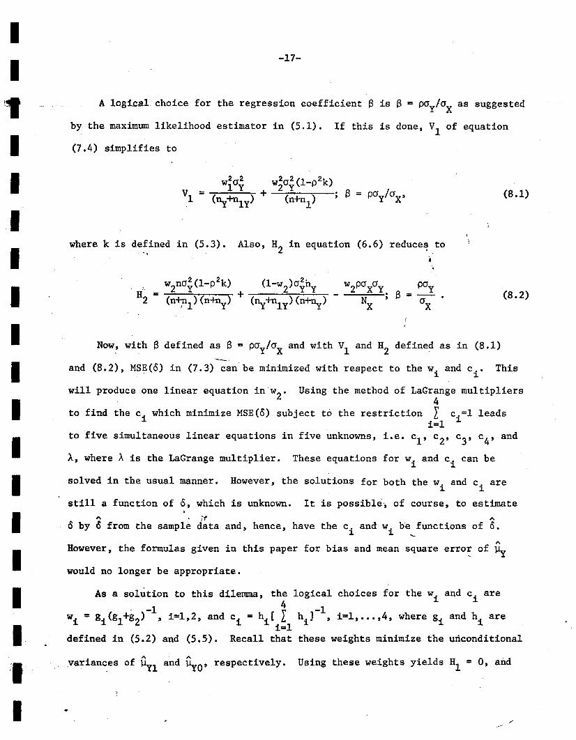
A logical choice for the regression coefficient B is B = (Xly/ax

as suggested

by the maximum likelihood estimator in (5.1). If this is done, VI of equation

(7.4) simplifies to

(8.1)

where k is defined in (5.3). Also, H2

in equation (6.6) reduces to

A ~ ;f A

o by 0 from the sample data and, hence, have the c. and w. be functions of O.1. 1.

A.

However, the formulas given in this paper for bias and mean square erro: of ~

would no longer be appropriate.

Now, with B defined as B = pay/ax and with VI and H2 defined as in (8.1)"--_.

and (8.2), MSE(o) in (7.3) can be minimized with respect to the w. and c .• This.1.1.

(8.2)

Using these weights yields HI = 0, and

logical choices for the wi and ci are

-1hi] , i=1, ••• ,4, where gi and hi are

these weights minimize the unconditional

the4

c i = hie li=l

Recall that

w2na~(1-p2k) (1-w2)a~~

H2= (n~l)(n+ny) + (Uy+nly)(n~)

Using the method of LaGrange multipliers4

the ci which minimize MSE(o) subject to the restriction l c.=l leadsi=l 1.

simultaneous linear equations in five unknowns, i.e. cl ' c2' c3 ' c4 ' andto five

to find

will produce one linear equation in w2 •

A, where A is the LaGrange multiplier. These equations for wi and ci can be

solved in the usual manner. However, the solutions for both the w. and c. are1. 1.

still a function of 0, which is unknown. It is possible, of course, to estimate

variances of Uyl and PyO ' respectively.

As a solution to this dilemma,. -1

wi = gi(gl+g2) , i=1,2, and

defined in (5.2) and (5.5).

IIIIIIIIII.'1

I

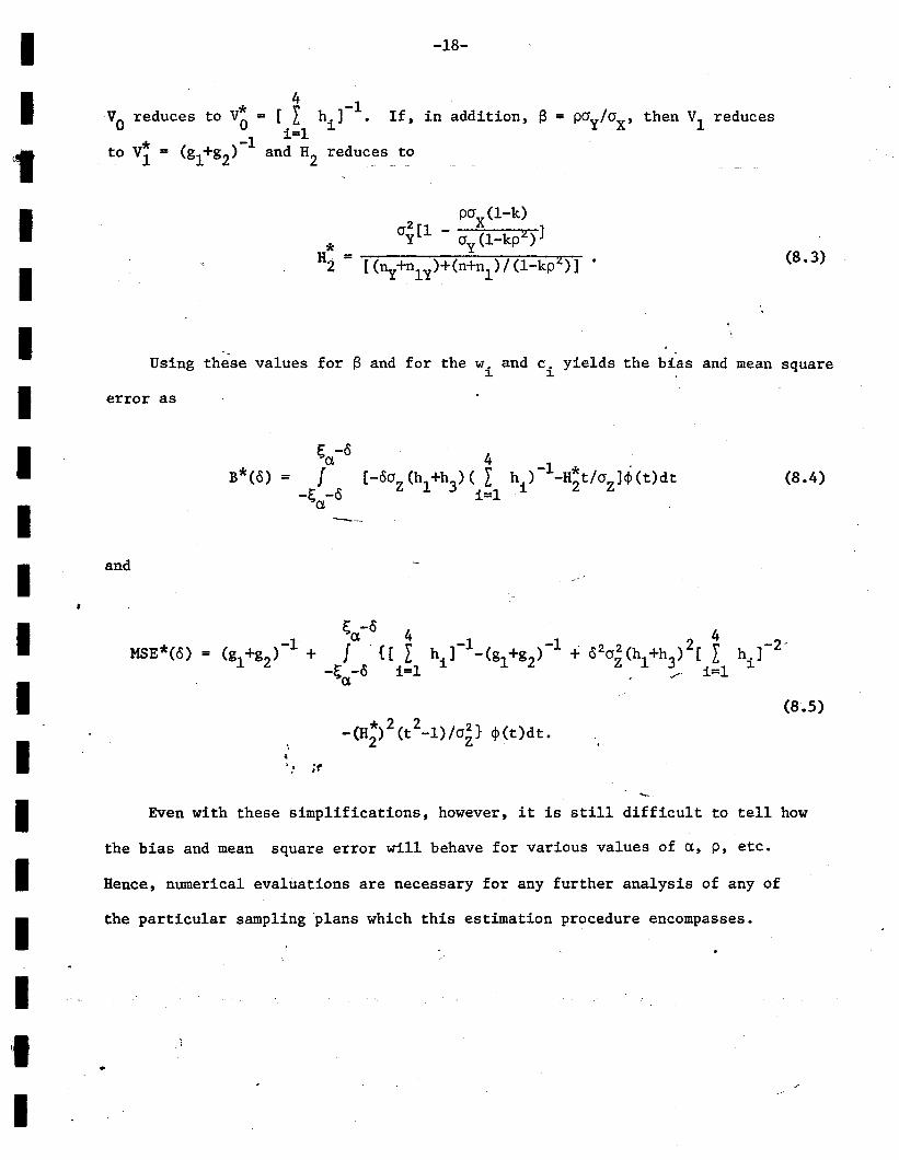
Even with these simplifications, however, it is still difficult to tell how

(8.3)

(8.4)

(8.5)

--

;t

~a-o

B*(o) = f-~a-o

-18-

"

Using these values for S and for the w. and c. yields the bias and mean square1. 1. •

* ~ -1Vo reduces to Vo = [L hi] • If, in addition, S = pay/aX' then Vl reducesi=l* -1to Vl = (gl+g2) and H2 reduces to

MSE*(o)

error as

and

the bias and mean square error will behave for various values of a, p, etc.

the particular sampling plans which this estimation procedure encompasses.

Hence, numerical evaluations are necessary for any further analysis of any of

IIl'IIIIIIIIIIIIII'II

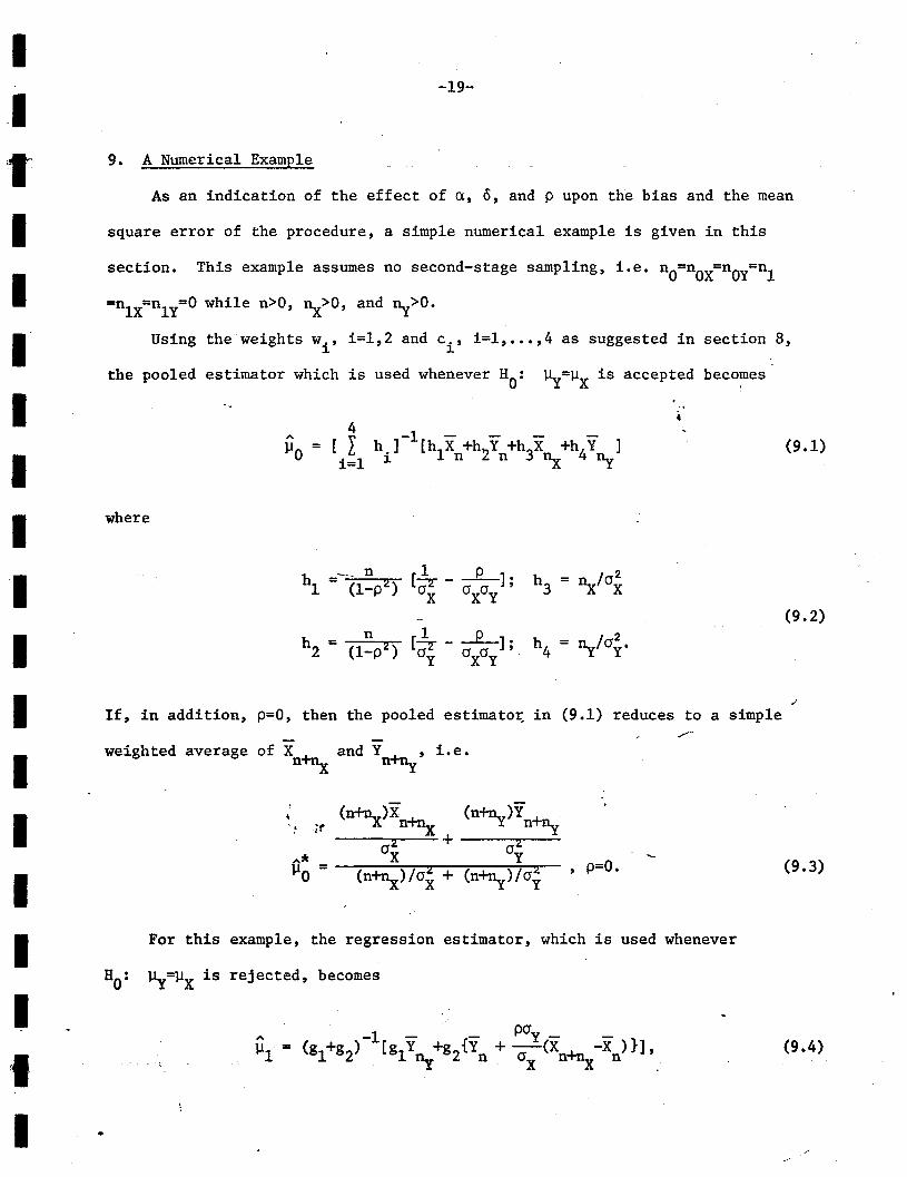
If, in addition, p=O, then the pooled estimato~ in (9.1) reduces to a simple

As an indication of the effect of a, 0, and p upon the bias and the mean

section. This example assumes no second-stage sampling, i.e. nO=nOX=nOy=n1

=nlX=nly=O while n>O, ~>O, and ~>O.

Using the weights w., i=1,2 and c., i=l, ••• ,4 as suggested in section 8,1 1

(9.1)

(9.2)

(9.3)

(9.4)

, p=O.

n 1 P 2h - [ ]. h4 = ~_/crY.2 - (l_p2) (1T - cra ' rY X Y

h --- n [1 p]1 = (1_p2) (1T - cra ;

X X Y

4nO = [l h.]-1[h

1X +h..,Y +h3X +h4Y ]

i=l 1 n ~ n nX ny

,.. 1 PC1y= (g +g ) - [glY +g2{Y + -(X +n.._-X )}],

~l 1 2 ny n aX n. --x n .'

For this example, the regression estimator, which is used whenever

-19-

the pooled estimator which is used whenever HO

: ~Y=~X is accepted becomes

square error of the procedure, a simple numerical example is given in this

9. A Numerical Example

where

weighted average of Xn+nx and Yn+ny' i.e.

HO: ~=~X is rejected, becomes

IIIIIIIIIIII

I

I.1fIIII

II'f

-20-

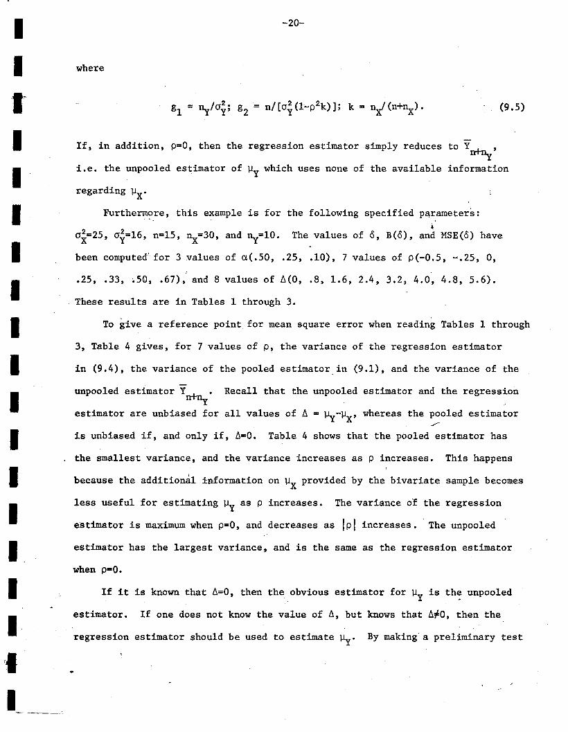
where

(9.5)

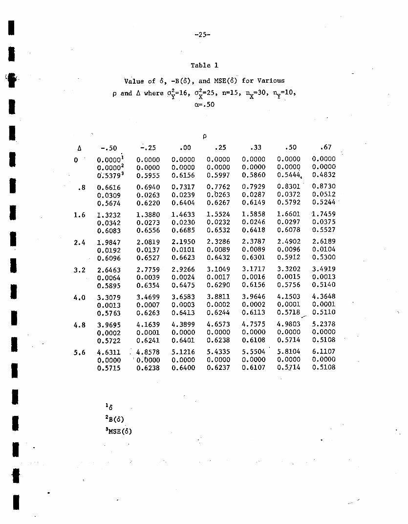
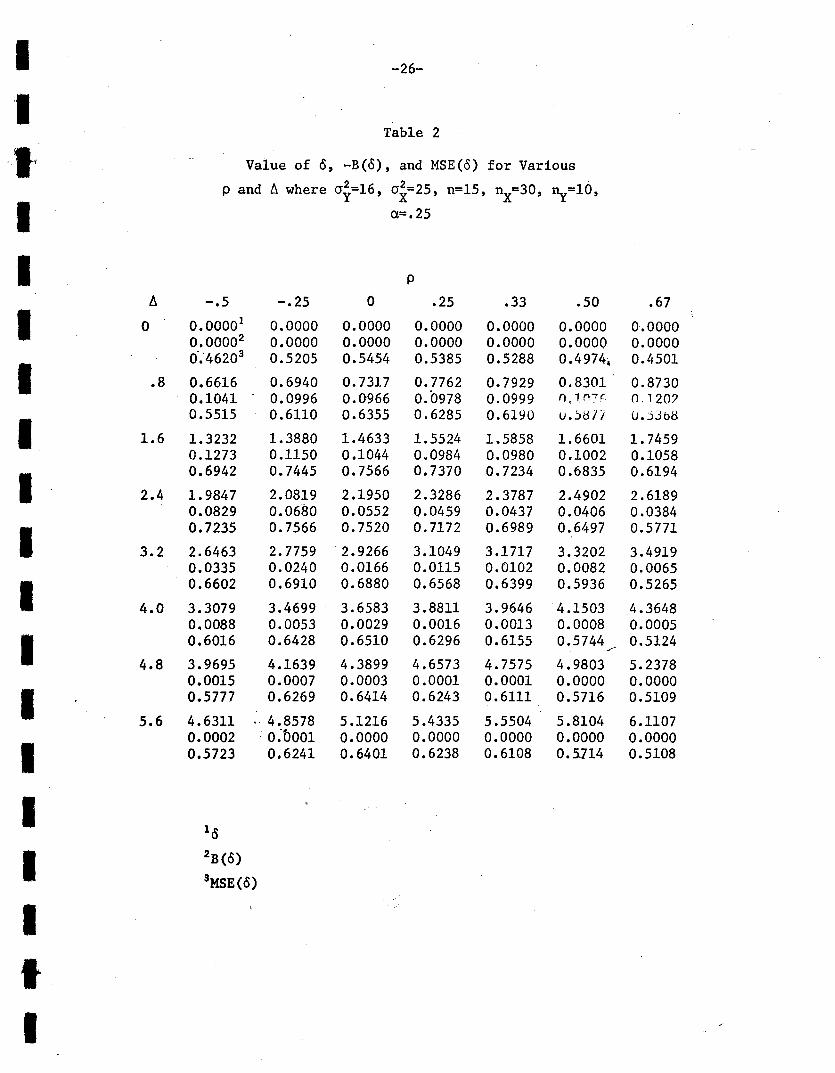
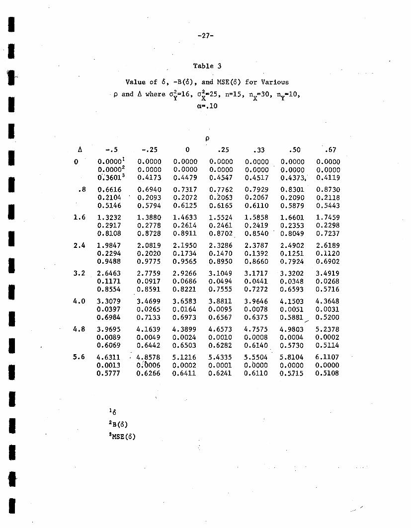
Furthermore, this example is for the following specified p~rameters:

been computed'for 3 values of <X(.50, .25, .10),7 values of p(-0.5, -.25,0,

If, in addition, p=O, then the regression estimator simply reduces to Yn+ny'

i.e. the unpoo1ed estimator of ~Y which uses none of the available information

regarding ~X'

IIII

0 2=25 0 2=16 n=15 ~_=30, and ~.=10.X 'Y' 'x y4

The values of 0, B(o), and MSE(o) have

IIIIIIIIII·'I

.25, .33, .50, .67), and 8 values of b.(0, .8,1.6,2.4,3.2,4.0,4.8,5.6).

These results are in Tables 1 through 3.

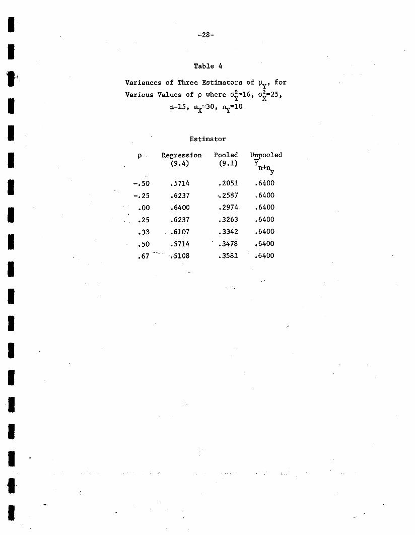
To give a reference point for mean square error when reading Tables 1 through

3, Table 4 gives, for 7 values of p, the variance of the regression estimator

in (9.4), the variance of the pooled estimator in (9.1), and the variance of the

unpoo1ed estimator Yn+ny' Recall that the unpoo1ed estimator and the regression

estimator are unbiased for all values of b. = ~Y-~X' whereas the pooled estimator

is unbiased if, and only if, b.=0. Table 4 shows that the pooled estimator has

the smallest variance, and the variance increases as p increases. This happens

because the additional information on ~X provided by the bivariate sample becomes

less useful for estimating ~Y as p increases. The variance of the regression

estimator is maximum when p=O, and decreases as Ipi increases. The unpoo1ed

estimator has the largest variance, and is the same as the regression estimator

when p=O.

If it is known that b.=0, then the obvious estimator for ~Y is the unpoo1ed

estimator. If one does not know the value of b., but knows that b.~0, then the

regression estimator should be used to estimate ~y' By making' a preliminary test

II

•IIIIIIIIIIIII'1JI

-21-

of significance, one expects to use the pooled estimator whenever ~~O or 0~0

and hence reduce the mean square error below the value of the variance (also

mean square error) of the regression estimator.

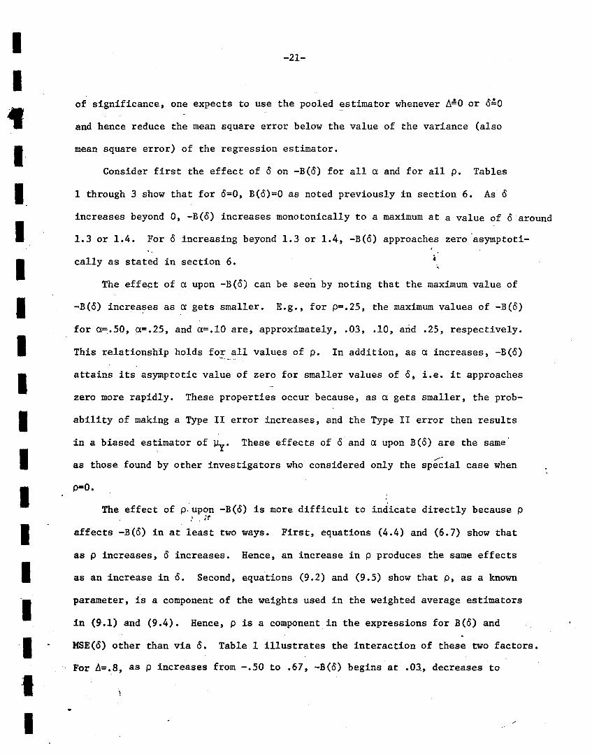
Consider first the effect of 0 on -B(o) for all a and for all p. Tables

1 through 3 show that for 0=0, B(o)=O as noted previously in section 6. As 0

increases beyond 0, -B(o) increases monotonically to a maximum at a value of 0 around

1.3 or 1.4. For o increasing beyond 1.3 or 1.4, -B(o) approaches zero 'asymptoti-

4cally as stated in section 6.

The effect of a upon -B(o) can be seen by noting that the maximum value of

-B(o) increa~es as a gets smaller. E.g., for p=.25, the maximum values of -B(O)

for a=.50, a=.25, and a=.lO are, approximately, .03, .10, arid .25, respectively.

This relationship holds for all values of p. In addition, as a increases, -B(o)

attains its asymptotic value of zero for smaller values of 0, i.e. it approaches

zero more rapidly. These properties occur because, as a gets smaller, the prob­

ability of making a Type II error increases, and the Type II error then results

in a biased estimator of ~Y. These effects of 0 and a upon B(o) are the same'

~

as those found by other investigators who considered only the special case when

p-O.

The effect of p.upon -B(o) is more difficult to indicate directly because p~ . ;t

affects -B(o) in at least two ways. First, equations (4.4) and (6.7) show that

as p increases, 0 increases. Hence, an increase in p produces the same effects

as an increase in o. Second, equations (9.2) and (9.5) show that p, as a known

parameter, is a component of the weights used in the weighted average estimators

in (9.l) and (9.4). Hence, p is a component in the expressions for B{o) and

MSE(o) other than via o. Table 1 illustrates the interaction of these two factors.

For ~=.8, as p increases from -.50 to .67, -B(o) begins at .03, decreases to

IIt·IIIIIIIIIIIIII

I

-22-

.02, and then increases to-.05. Now, if p were having no effect over and above

its effect through 0, then -B(o) should steadily increase as p increases because

o is increasing from .66 to .87. This isn't true, however, since -B(o) decreases

until p attains some point in the interval [O,~). For ~=1.6 in Table 1, one

would expect -B(o) to decrease as p increases if p was having its only effect

through o. However, -B(o) decreases until p reaches a point in [O,~), and then

it begins to increase. The same general behavior is seen for ~=2.4, although

the minimum value of -B(o) appears to occur for p E [~,~J. For ~~3.2 in Table 1,

an increase in p produces a decrease in -B-(o), most likely primarily through the

influence of o. S~ilar patterns are seen in Tables 2 and 3, except that the

value of ~ for which an increase in p always produces a decrease in -B(o) gets

smaller as a gets smaller (i.e. ~=3.2, 2.4, and 1.6 in Tables 1, 2, ,and 3, res­

pectively). In general, it appears from this example that an increase in p

will cause the same effects as an increase in 0, with the following exceptions:

1) For 0 in the range of, approximately 0 to .7, an increase in p produces

a decrease in -B(o) rather than an increase. /

2) For 0 in the range of, approximately, 1.6 to 1.8, an increase in p

produces an increase in -B(o) rather than a decrease.

Consider now the effect of 0 on MSE(o) for any given value of p and a.-,J.

Looking down any column of Tables 1, 2, or 3, it can be seen that the minimum'-

MSE(o) occurs at 0=0. This minimum value of MSE(o) is less than the variance

of the regression estimator, but greater than the variance of the pooled

estimator. As 0 increases beyond 0, MSE(o) increases monotonically until it

reaches the value of the variance of the regression estimator. This occurs

approximately around 0=.8. As 0 increases beyond .8, MSE(o) increases monotonically

until it attains its maximum value for 0 approximately equal to 2. As 0

IItIIIIIIIIIIIIII,I

I

-23-

increases beyond 2, MSE(o) decreases monotonically toward a limiting

- value which is the variance of the regression estimator. Hence, the pooling

procedure yields maximum mean square error around 0=2, with MSE(o) approaching

from above the variance of the regression estimator for 0>2 and MSE(o) less

than the variance of the regression estimator for 0<.8 (approximately).

The effect of a upon MSE(o) can be seen by noting that, for fixed p, the

minimum value of MSE(o) decreases as a decreases. E.g., for p=.25, the,minimum

value of MSE(o) is .60, .54, and .45 for a=.50, .25, and .10, re~pectively. Also,

the maximum value of MSE(o) increases as a·decreases. E.g., for p=.25, the

maximum values of MSE(o) are (approximately) .65, .74, and .90 for a=.50, .25,

and .10, respectively. In addition, it can be noted from Tables 1 through 3

that, as a decreases, MSE(o) approaches its asymptotic value more slowly.--._~

Hence, a smaller value of a will result in a larger reduction in MSE(o) if 0

is small (approximately less than .S), but, on the other hand, will result in

a larger increase in MSE(o) if 0 is moderate (approximately equal to 2). These

effects of 0 and a upon MSE(o) are the same as those found by other investigators

for the special cases where p=O. ...,-.

P can affect MSE(o) either via 0 or through its influence on the weights

in the weighted estimators. The general effect upon MSE(o) of increasing p;~

from -.50 to .67, as illustrated in Tables 1 through 3, is to first increase

MSE(o) to some maximum value and then to decrease MSE(o). For any given value of

~, Table 1 shows that the maximum value for MSE(o) is attained for p approximately

equal to zero, whereas in Tables 2 and 3 the maximum value for MSE(o) is attained

for some value of p in the interval (-.25,.25). Hence, in general, it appears

that an increase in the absolute value of p will decrease MSE(o), altnough this

relationship between p and MSE(o) is definitely not symmetric about the point p=O.

IIfIIIIIIIIIIIIIIII

-24-

10. Some General Conclusions

The bias and mean square error of a two-stage sampling scheme which involves

a preliminary test of significance have been derived. Numerical investigation

of some one-stage examples only indicate that in this procedure a and 0 have an

effect on B(o) and MSE(o) which is similar to that reported by other authors

who have considered similar procedures. In addition, it appears that an increase

in the absolute value of p will generally decrease MSE(o). The relationship

between p and"B(o) is not obvious, but it appears that p influenCes B(o) primarily

through the effect of p upon o.

/

I -25-

ITable 1

(t Value of 0, -B(o), and MSE(o) for Various

p and ~ where 0 2=16 0 2=25 n=15 ~=30 ny=10

Iy 'X' , , ,

cx=.50

I p

~ -.50 -.25 .00 .25 .33 .50 .67

I 0 0.0000 1 0.0000 0.0000 0.0000 0.0000 0.0000 0.00000.00002 0.0000 0.0000 0.0000 0.0000 O.oooq 0.0000

I0':5379 3 0.5955 0.6156 0.5997 0.5860 0.54444

0.4832

.8 0.6616 0.6940 0.7317 0.7762 0.7929 0.8301 0.87300'.0309 0.0263 0.0239 0.b263 0.0287 0.0372 0.0512

I0.5674 0.6220 0.6404 0.6267 0.6149 0.5792 0.5244 .

1.6 1.3232 1. 3880 1.4633 1.5524 1.5858 1.6601 1. 74590.0342 0.0273 0.0230 0.0232 0.0246 0.0297 0.0375

I0.6083 0.6556 0.6685 0.6532 0.6418 0.6078 0.5527

2.4 1. 9847 2.0819 2.1950 2.3286 2.3787 2.4902 2.61890.0192 0.0137 0.0101 0.0089 0.0089 0.0096 0.0104

I0.6096 0.6527 0.6623 0.6432 0.6301 0.5912 0.5300

3.2 2.6463 2.7759 2.9266 3.1049 3.1717 3.3202 3.49190.0064 0.0039 0.0024 0.0017 0.0016 0.0015 0.0013

I 0.5895 0.6354 0.6475 0.6290 0.6156 0.5756 0.5140

4.0 3.3079 3.4699 3.6583 3.8811 3.9646 4.1503 4.36480.0013 0.0007 0.0003 0.0002 0.0002 0.0001 0.0001

I 0.5763 0.6263 0.6413 0.6244 0.6113 0.5718 0.5110./

4.8 3.9695 4.1639 4.3899 4.6573 4.7575 4.9803 5.23780.0002 0.0001 0.0000 0.0000 0.0000 0.0000 0.0000

I 0.5722 0.6241 0.6401 0.6238 0.6108 0.5714 0.5108

5.6 4.6311 4.8578 5.1216 5.4335 5.5504 5.8104 6.1107

I0.0000 '. 0.'0000 0.0000 0.0000 0.0000 0.0000 0.00000.5715 0.6238 0.6400 0.6237 0.6107 0.5]14 0.5108

I 10

I 2B(O)

sMSE(o)

III

I -26-

ITable 2

t Value of 0, -B(o), and MSE(o) for Various

Ip and ~ where cr~=16, cr~=25, n=15, nX=30, ny=10,

a=.25

I p

f:. -.5 -.25 0 .25 .33 .50 .67

I 0 0.0000 1 0.0000 0.0000 0.0000 0.0000 0.0000 0,.00000.00002 0.0000 0.0000 0.0000 0.0000 0.0000 0.0000

I0':46203 0.5205 0.5454 0.5385 0.5288 0.4974, 0.4501

.8 0.6616 0.6940 0.7317 0.7762 0.7929 0.8301 0.87300.1041 0.0996 0.0966 0.0978 0.0999 () • 1 ('17 F- a 120?

I0.5515 0.6110 0.6355 0.6285 0.6190 u.j81l O.SJbB

1.6 1.3232 1.3880 1.4633 1.5524 1.5858 1.6601 1.74590.1273 0.1150 0.1044 0.0984 0.0980 0.1002 0.1058

I0.6942 0.7445 0.7566 0.7370 0.7234 0.6835 0.6194

2.4 1.9847 2.0819 2.1950 2.3286 2.3787 2.4902 2.61890.0829 0.0680 0.0552 0.0459 0.0437 0.0406 0.0384

I0.7235 0.7566 0.7520 0.7172 0.6989 0.6497 0.5771

3.2 2.6463 2.7759 2.9266 3.1049 3.1717 3.3202 3.49190.0335 0.0240 0.0166 0.0115 0.0102 0.0082 0.0065

I 0.6602 0.6910 0.6880 0.6568 0.6399 0.5936 0.5265

4.0 3.3079 3.4699 3.6583 3.8811 3.9646 '4.1503 4.36480.0088 0.0053 0.0029 0.0016 0.0013 0.0008 0.0005

I 0.6016 0.6428 0.6510 0.6296 0.6155 0.5744 0.5124.----4.8 3.9695 4.1639 4.3899 4.6573 4.7575 4.9803 5.2378

0.0015 0.0007 0.0003 0.0001 0.0001 0.0000 0.0000

I 0.5777 0.6269 0.6414 0.6243 0.6111 0.5716 0.5109

5.6 4.6311 4.8578 5.1216 5.4335 5.5504 5.8104 6.11070.0002 . O:bOOl 0.0000 0.0000 0.0000 0.0000 0.0000

I ' 0.5723 0.6241 0.6401 0.6238 0.6108 0.5114 0.5108

I 10

I 2B(0)

3MSE (0)

IfI

IIIJ{

IIIIIIIIIII,I

II,I,

I

-28-

Table 4

Variances of Three Estimators of ~Y' for

Various Values of p where cr~=16, cr~=25,

n=15, ~=30, ny=lO

Estimator

p Regression Pooled Unpooled(9.4) (9.1) Yn+n

y

-.50 .5714 .2051 .6400

-.25 .6237 ·.2587 .6400

.00 .6400 .2974 .6400

.25 .6237 .3263 .6400

.33 .6107 .3342 .6400

.50 .5714 .3478 .6400

.67 ---, '.5108 .3581 .6400

III"IIIIIIIIIIIIIIII

[1]

[2]

[3]

[4]

[5]

[6]

[7]

[8]

[9]

[10]

[11]

[12]

[13]

[14]

. (15]

-29-

REFERENCES

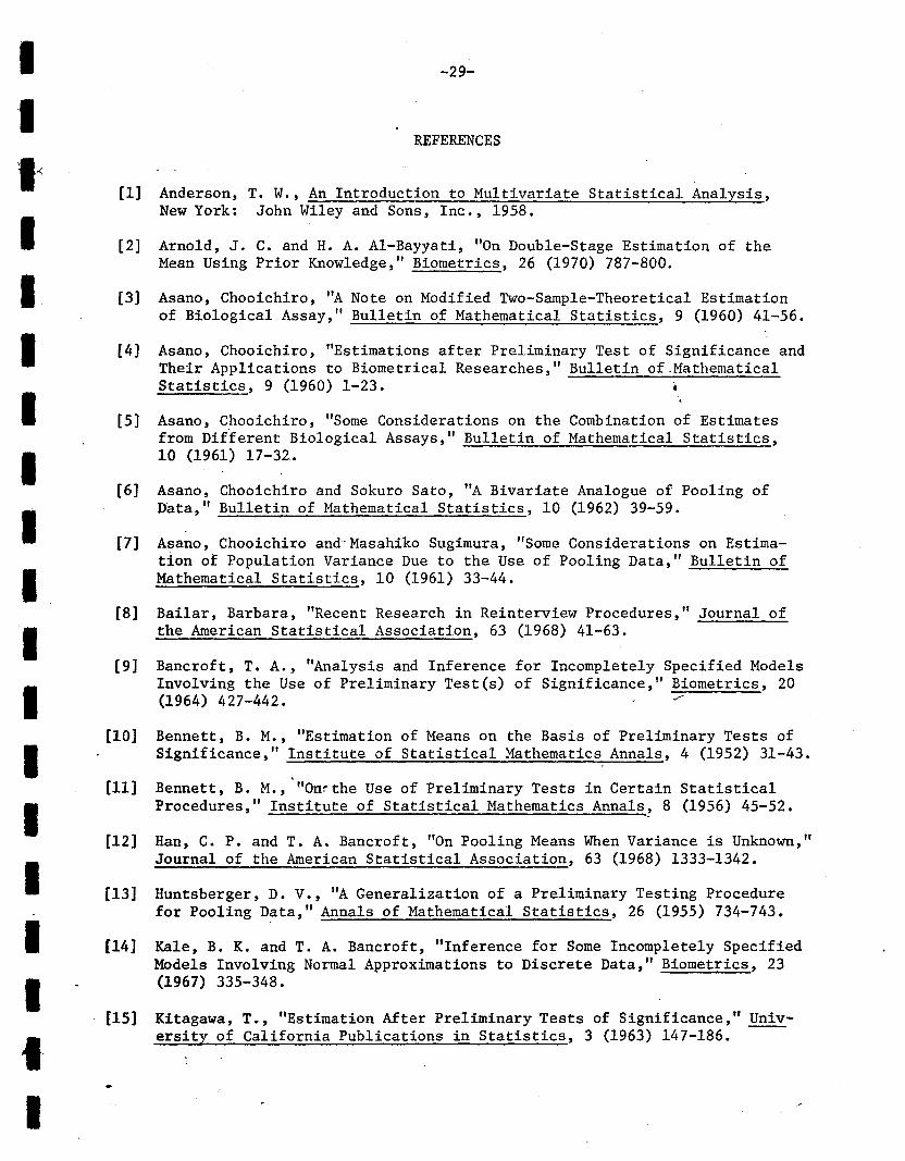
Anderson, T. W., An Introduction to Multivariate Statistical Analysis,New York: John Wiley and Sons, Inc., 1958.

Arnold, J. C. and H. A. Al-Bayyati, "On Double-Stage Estimation of theMean Using Prior Knowledge," Biometrics, 26 (1970) 787-800.

Asano, Chooichiro, '~ Note on Modified Two-Sample-Theoretical Estimationof Biological Assay," Bulletin of Mathematical Statistics, 9 (1960) 41-56.

Asano, Chooichiro, "Estimations after Preliminary Test of Significance andTheir Applications to Biometrical Researches," Bulletin of.MathematicalStatistics, 9 (1960) 1-23.

Asano, Chooichiro, "Some Considerations on the Combination of Estimatesfrom Different Biological Assays," Bulletin of Mathematical Statistics,10 (1961) 17-32.•

Asano, Chooichiro and Sokuro Sato, "A Bivariate Analogue of Pooling ofData," Bulletin of Mathematical Statistics, 10 (1962) 39-59.

Asano, Chooichiro and-Masahiko Sugimura, "Some Considerations on Estima­tion of Population Variance Due to the Use of Pooling Data," Bulletin ofMathematical Statistics, 10 (1961) 33-44.

Bailar, Barbara, "Recent Research in Reinterview Procedures," Journal ofthe American Statistical Association, 63 (1968) 41-63.

Bancroft, T. A., "Analysis and Inference for Incompletely Specified ModelsInvolving the Use of Preliminary Test(s) of Significance," Biometrics, 20(1964) 427-442. ./

Bennett, B. M., "Estimation of Means on the Basis of Preliminary Tests ofSignificance," Institute of Statistical Mathematics Annals, 4 (1952) 31-43.

Bennett, B. M., •"On~ the Use of Preliminary Tests in Certain StatisticalProcedures," Institute of Statistical Mathematics Annals, 8 (1956) 45-52.

Han, C. P. and T. A. Bancroft, "On Pooling Means When Variance is Unknown,"Journal of the American Statistical Association, 63 (1968) 1333-1342.

Huntsberger, D. V., "A Generalization of a Preliminary Testing Procedurefor Pooling Data," Annals of Mathematical Statistics, 26 (1955) 734-743.

Kale, B. K. and T. A. Bancroft, "Inference for Some Incompletely SpecifiedModels Involving Normal Approximations to Discrete Data," Biometrics, 23(1967) 335-348.

Kitagawa, T., "Estimation After Preliminary Tests of Significance," Univ­ersity of California Publications in Statistics, 3 (1963) 147-186. ----

II~

IIIIIIIIIIIIIIII

-30-

[16] Mehta, J. S. and John Gurland, "Testing Equality of Means in the Presenceof Correlation," Biometrika, 56 (1969) 119-126.

[17] Mosteller, F., "On Pooling Data," Journal of the American StatisticalAssociation, 43 (1948) 231-242.

[18] Ruhl, D. J. B., Preliminary Test Procedures and Bayesian Procedures forPooling Correlated Data, unpublished Ph.D Dissertation, Ames, Iowa:Iowa State University, 1967.

[19] Sato, Sokuro, "A Multivariate Analogue of Pooling of Data," Bulletin ofMathematical Statistics, 10 (1962) 61-76.

[20] Tamura, Ryoji, "Nonparametric Inferences with a Preliminary. Test," Bulletinof Mathematical Statistics, 11 (1965) 39-61. •

[21] Tamura, Ryoji, ~'Some Estimate Procedures with a Nonparametric PreliminaryTest I," Bulletin of Mathematical Statistics, 11 (1965) 63-71.

[22] Yen, Elizabeth, "On Two State Non-Parametric Estimation," Annals of Math­ematical Statistics, 35 (1964) 1099-1114.