Embed Size (px)
Citation preview

ISR develops, applies and teaches advanced methodologies of design and analysis to solve complex, hierarchical,heterogeneous and dynamic problems of engineering technology and systems for industry and government.
ISR is a permanent institute of the University of Maryland, within the Glenn L. Martin Institute of Technol-ogy/A. James Clark School of Engineering. It is a National Science Foundation Engineering Research Center.
Web site http://www.isr.umd.edu
I RINSTITUTE FOR SYSTEMS RESEARCH
TECHNICAL RESEARCH REPORT
Closed-Loop Monitoring Systems for Detecting Incipient Instability
by T. Kim, E. Abed
T.R. 98-49

Report Documentation Page Form ApprovedOMB No. 0704-0188
Public reporting burden for the collection of information is estimated to average 1 hour per response, including the time for reviewing instructions, searching existing data sources, gathering andmaintaining the data needed, and completing and reviewing the collection of information. Send comments regarding this burden estimate or any other aspect of this collection of information,including suggestions for reducing this burden, to Washington Headquarters Services, Directorate for Information Operations and Reports, 1215 Jefferson Davis Highway, Suite 1204, ArlingtonVA 22202-4302. Respondents should be aware that notwithstanding any other provision of law, no person shall be subject to a penalty for failing to comply with a collection of information if itdoes not display a currently valid OMB control number.
1. REPORT DATE 09 SEP 1998 2. REPORT TYPE
3. DATES COVERED 00-00-1998 to 00-00-1998
4. TITLE AND SUBTITLE Close-Loop Monitoring Systems for Detecting Incipient Instability
5a. CONTRACT NUMBER
5b. GRANT NUMBER
5c. PROGRAM ELEMENT NUMBER
6. AUTHOR(S) 5d. PROJECT NUMBER
5e. TASK NUMBER
5f. WORK UNIT NUMBER
7. PERFORMING ORGANIZATION NAME(S) AND ADDRESS(ES) Department of Electrical Engineering,Institute for SystemsResearch,University of Maryland,College Park,MD,20742
8. PERFORMING ORGANIZATIONREPORT NUMBER
9. SPONSORING/MONITORING AGENCY NAME(S) AND ADDRESS(ES) 10. SPONSOR/MONITOR’S ACRONYM(S)
11. SPONSOR/MONITOR’S REPORT NUMBER(S)
12. DISTRIBUTION/AVAILABILITY STATEMENT Approved for public release; distribution unlimited
13. SUPPLEMENTARY NOTES
14. ABSTRACT see report
15. SUBJECT TERMS
16. SECURITY CLASSIFICATION OF: 17. LIMITATION OF ABSTRACT
18. NUMBEROF PAGES
37
19a. NAME OFRESPONSIBLE PERSON
a. REPORT unclassified
b. ABSTRACT unclassified
c. THIS PAGE unclassified
Standard Form 298 (Rev. 8-98) Prescribed by ANSI Std Z39-18

Closed-Loop Monitoring Systems for
Detecting Incipient Instability
Taihyun Kim and Eyad H. Abed
Department of Electrical Engineering
and the Institute for Systems Research
University of Maryland
College Park, MD 20742 USA
Manuscript: 9 September 1998
Abstract
Monitoring systems are proposed for the detection of incipient instability in uncer-
tain nonlinear systems. The work employs generic features associated with the response
to noise inputs of systems bordering on instability. These features, called \noisy pre-
cursors" in the work of Wiesenfeld, also yield information on the type of bifurcation
that would be associated with the predicted instability. The closed-loop monitoring
systems proposed in the paper have several advantages over simple open-loop moni-
toring. The advantages include the ability to in uence the frequencies at which the
noisy precursors are observed, and the ability to simultaneously monitor and control
the system.
1 Introduction
In this paper, we propose monitoring systems for detection of incipient instability in uncertainnonlinear systems. Our aim is to develop automatic monitoring systems that provide awarning that a system is operating dangerously close to an instability. Such a warningmechanism can be of great value especially when no accurate system model is available andthe system is being operated in a stressed condition. If an exact model were available, then
1
the stability boundary could be calculated o�-line, and there would be no need for an on-linemonitoring system for detecting incipient instability.
Generically, loss of stability results in bifurcation of new steady states from the nominalone [6], [17],[19]. The type of bifurcation that occurs depends on the manner in which thesystem loses stability. Since bifurcations involve changes neglected in linearized models, it isnot surprising that linear control design methods have often been found to be inadequate forcontrol law design for stressed systems. Bifurcation control methods have arisen to addressstabilization of systems in such situations [4].
In this paper, we contribute to this problem area by considering the design of monitoringsystems for detection of incipient instability. We also make observations on the design ofcombined monitoring and control systems for physical systems susceptible to bifurcation andloss of stability.
To develop an on-line approach to the detection of incipient instability in the absence of anaccurate system model, we harness the e�ects of external continuously acting disturbances.The presence of these disturbances facilitates determination of measured signal featuresassociated with nearness to instability. The presence of disturbance inputs, which can occurnaturally or be injected, is crucial. Without continuous disturbances, a system at equilibriumwould remain at equilibrium until an instability occurs, with no possibility of an on-linewarning signal. We take the continuously acting disturbances to be white noise inputs. Thisallows us to make use of previous work of Wiesenfeld and co-workers [20, 11, 21, 22, 24, 14, 23].Wiesenfeld was interested in features that can be observed in the power spectrum of ameasured output of a system that is operating close to an incipient bifurcation. He focused onnonlinear systems operating along a steady state limit cycle. He referred to the distinguishingfeatures in the power spectrum as \noisy precursors" of the bifurcations. Noisy precursorsare aspects of the power spectral density of a measured output that arise in the vicinity ofan instability.
The monitoring systems we propose do not employ or require a system model. Rather,use of the noisy precursors notion allows a nonparametric approach based on general featuresof noise-driven systems operating close to instability. Moreover, the monitoring systems wedevelop are closed-loop, in the sense that they involve both sensing and actuation. Thishas important advantages over the direct open-loop approach of simply monitoring a systemoutput and deciding if it exhibits features of a noisy precursor. Closed-loop monitoringsystems can enhance our con�dence in deciding that system operation is indeed near aninstability as well as in determining the nature of the instability.
For many engineering system models, the normal operating condition is an equilibriumpoint rather than a periodic solution. Thus, we extend the theory of noisy precursors tosystems operating at an equilibrium point. This forms the basis for our design of monitoring
2

systems for detection of incipient instability.Our results apply to situations that share the following general characteristics. A physical
system is operating at or near a nominal stable steady state. The system depends on a setof parameters, some of which change slowly with time. Outside a certain range of parametervalues (the \design range"), model uncertainty impedes reliable determination of systemstability. However, there are circumstances in which the parameters will move outside ofthe design range. Moreover, in these circumstances it is crucial that system operability bemaintained as far as possible outside the design range. The parameter changes may occurdue to action of the system operator, or may be exogenous. We refer to operation outsidethe design range as \stressed operation."
There are many important examples in which systems need to be operated in o�-design,stressed conditions. The driving factors depend on the application, but in general they entaila desire to achieve increased performance without re-design or expansion of the system.Often, stressed operation leads to a reduced margin of stability. Thus, stressed operationcan be unsafe, in that small uncertainties or disturbances can lead to loss of stability, i.e.,to system failure. Examples include electric power system voltage collapse [18], chemicalreactor runaway [12], jet engine stall [13], aircraft stall at high angle-of-attack [5], and lasersystem instability [8]. For each of these examples, precise models are di�cult to obtain,especially outside the design range.
The paper is organized as follows. In Section 2, we study noisy precursors for instabilityfor systems operating at an equilibrium point. In Section 3, we introduce a basic monitoringsystem that facilitates use of precursors to detect incipient instability. In Section 4, weredesign the monitoring system to ensure that the bifurcation occurring in the overall systemis supercritical. The monitoring systems of Section 3 and Section 4 require full state feedback.In Section 5, we alleviate the full state feedback requirement for plants that can be viewedas singularly perturbed (two time-scale) systems. In Section 6, we relax another assumption,namely that the system equilibrium point is known. In Section 7, we give a simple example.In Section 8, we collect our conclusions.
2 Noisy Precursors for Nonlinear System Instabilities
In this section, we extend the noisy precursor analysis of Wiesenfeld [20] to systems operatingat an equilibrium point. Wiesenfeld considered systems driven by white noise and operatingnear a periodic steady state. He showed that the power spectrum of a measured outputfor such a system exhibits sharply growing peaks near certain frequencies as the systemnears a bifurcation. The particulars depend on the type of bifurcation that the system
3

was approaching. He used the results to show that bifurcating systems could be used asselective-frequency ampli�ers [11], [22], [23].
Consider a nonlinear dynamic system (\the plant")
_~x = f(~x; �) +N(t) (1)
where ~x 2 Rn, � is a bifurcation parameter, and N(t) 2 Rn is a zero-mean vector whiteGaussian noise process. Let the system possess an equilibrium point ~x0. For small pertur-bations and noise, the dynamical behavior of the system can be described by the linearizedsystem in the vicinity of the equilibrium point ~x0. The linearized system corresponding to(1) with a small noise forcing N(t) is given by
_x = Df(~x0; �)x+N(t) (2)
where x := ~x � ~x0 and N(t) 2 Rn is a vector white Gaussian noise having zero mean. Forthe results of the linearized analysis to have any bearing on the original nonlinear model,we must assume that the noise is of small amplitude. This assumption of small noise will beexplicated below, in terms of smallness of correlation and cross-correlation coe�cients. Thedistinct notation for the system state ~x and the linearized system state x was used here forclarity. In the sequel, we will simply use the notation x and the meaning will be clear fromthe context.
The noise N(t) can occur naturally or can be injected using available controls. To facili-tate consideration of cases in which the noise is intentionally injected, we write N(t) in thegeneral form
N(t) = Bn(t) (3)
where B 2 Rn�m and n(t) 2 Rm is a vector white Gaussian noise. This notation allowsus to easily consider cases in which noise is injected in di�erent equations through availableactuation means. The noise vector N(t) is a white Gaussian with zero mean as long as n(t)is a white Gaussian with zero mean.
We view the system (2) as being in steady state and driven only by the noise process.Thus, we solve for the evolution of the state assuming a zero initial condition. The solutionof equation (2) at time t with a zero initial condition is
x(t) = eAtZ t
0e�AsN(s)ds (4)
where A := DF (x0). For our analysis, we assume that x0 is an asymptotically stableequilibrium point, i.e., all the eigenvalues of A have negative real part. We can express (4)
4

in terms of the eigenvectors and eigenvalues of A (normalized, and assumed distinct):
x(t) =nX
j=1
ljZ t
0
nXk=1
lkN(s)e�ksrkdse�jtrj
lirj = �ij
where ri and li are right and left eigenvectors, respectively, of A corresponding to eigenvalue�i, and where �ij is the Kronecker delta:
�ij =
(0 i 6= j
1 i = j(5)
Thus, the i-th component of x(t) is given by
xi(t) =nX
j=1
e�j trji
Z t
0ljN(s)e��jsds (6)
Since the power spectrum is the Fourier transform of the autocovariance function, we calcu-late the autocovariance for xi(t):
hxi(t)xi(t+ �)i =nX
j=1
nXk=1
e�j te�k(t+�)rji r
ki
Z t+�
0
Z t
0e��js1e��ks2
�nX
o=1
nXp=1
ljolkphNo(s1)Np(s2)ids1ds2
Let the noise have autocorrelation function
hNi(t)Nj(t+ �)i = �ij�(�) (7)
where �(�) is the Dirac delta function and the �ij are constants for all i; j. Moreover, �ijshould be small enough such that linearized analysis is valid. Again, (7) is satis�ed for thelinearized system as long as n(t) satis�es
hni(t)nj(t+ �)i = ij�(�) (8)
where the ij are constants for all i; j. Then
hxi(t)xi(t+ �)i =nX
j=1
nXk=1
e�j te�k(t+�)rji r
ki
Z t+�
0
Z t
0e��js1e��ks2
5

�nX
o=1
nXp=1
ljolkp�op�(s1 � s2)ds1ds2
=nX
j=1
nXk=1
e�j te�k(t+�)rji r
ki
Z t
0e��jse��ks
�nX
o=1
nXp=1
ljolkp�opds (9)
Note that the upper limit of integration changes from t+� to t because the impulse �(s1�s2)occurs for s1 = s2, and s1 < t in the inner integral.
For a dynamic system that depends on a single parameter, there are two basic typesof bifurcation from an equilibrium point. One is stationary bifurcation in which a newequilibrium emerges or the original equilibrium point suddenly disappears at the bifurcation.The other is Hopf bifurcation, where a periodic orbit emerges from the equilibrium pointat bifurcation. In stationary bifurcation, a real eigenvalue of the linearized system becomeszero as the parameter varies. In Hopf bifurcation, a complex conjugate pair of eigenvaluescrosses the imaginary axis.
Consider �rst the Hopf bifurcation. Assume that a complex conjugate pair of eigenvalues(denote them as � � �1; �� � �2) close to the imaginary axis has relatively smaller negativereal part in absolute value compared to other system eigenvalues:
jRe(�1)j; jRe(�2)j � jRe(�i)j (10)
for i = 3; : : : ; n. Since the integrand in (9) is the product of decaying exponentials (due tothe asymptotic stability assumption) and bounded, terms involving �1 and �2 dominate (9)for large t:
hxi(t)xi(t+ �)i � e�1(2t+�)(r1i )2Z t
0e�2�1s
nXj=1
nXk=1
l1j l1k�ijds
+ e�2(2t+�)(r2i )2Z t
0e�2�2s
nXj=1
nXk=1
l2j l2k�ijds
+ e�1(t+�)+�2tr1i r2i
Z t
0e�(�1+�2)s
nXj=1
nXk=1
l1j l2k�ijds
+ e�2(t+�)+�1tr1i r2i
Z t
0e�(�1+�2)s
nXj=1
nXk=1
l1j l2k�ijds
The power spectrum is measured with the use of a spectrum analyzer, and most practicalspectrum analyzers perform both an ensemble average and a time average. Thus, the �nal
6

autocovariance function is
Cii(�) := Re[hxi(t)xi(t + �)it] (11)
� � � 2e���
�cos(!�) + � � [e
��� (� cos(!�)� ! sin(!�))
2(�2 + !2)] (12)
where �t indicates averaging over time t, and we have written Cii in terms of �; ! > 0 insteadof in terms of �1 = �� + j! and �2 = ��� j!. Also, � and � are
� :=nX
j=1
nXk=1
l1j l2k�jkr
1i r
2i
� :=nX
j=1
nXk=1
l1j l1k�jk(r
1i )
2 +nX
j=1
nXk=1
l2j l2k�jk(r
2i )
2
Finally, taking the Fourier transform of equation (12) yields the desired power spectrum:
Sii(�) = �(j� + �)
(j� + �)2 + !2
+ �[�(j� + �)
(�2 + !2)((j� + �)2 + !2))� 1
(�2 + !2)((j� + �)2 + !2))] (13)
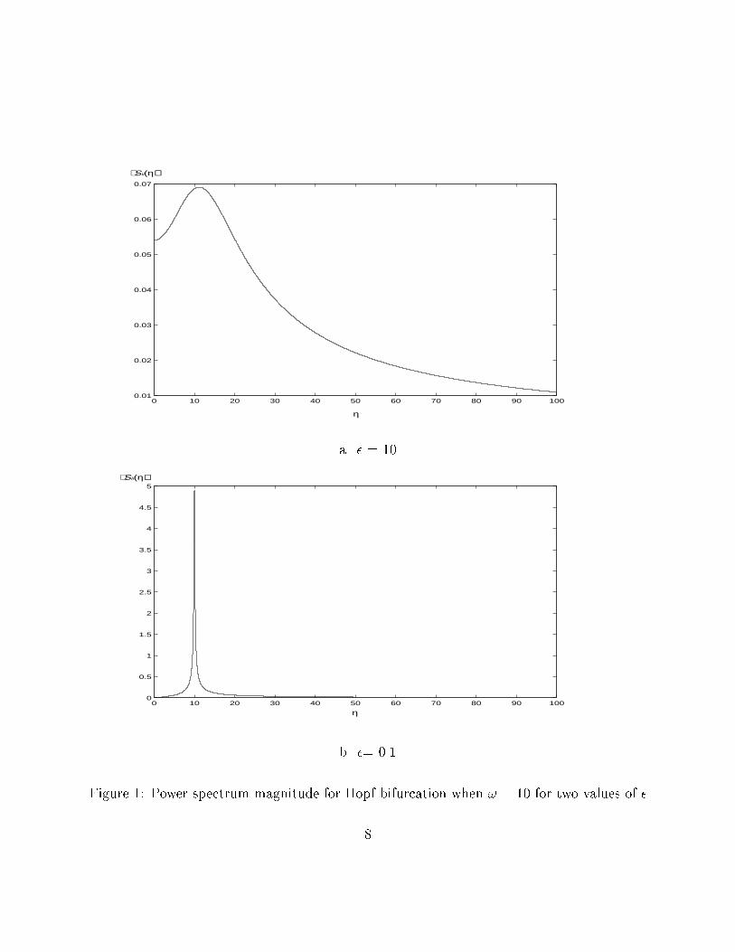
The magnitude of Sii(�) is maximum at � = ! and the maximum grows without bound as� ! 0. Moreover, as the noise power (as measured by the �ij) increases, the magnitudeof Sii(�) also increases. However, since � and � a�ect Sii(�) linearly and uniformly overfrequency �, the shape of the magnitude Sii(�) doesn't change with increasing noise power.Of course, we have assumed that the noise is of small amplitude, so we cannot actually allowthe �ij to increase without bound.
Fig. 1 shows the magnitude of Sii(�) for ! = 10, for two values of �. (For de�niteness, �and � have been set to 1 in constructing Fig. 1.) Note the sharp peak around ! = 10 thatappears as � ! 0. From this observation, we can conclude that the power spectrum peaknear the bifurcation is located at !, and the magnitude of this peak grows as � approaches tozero. This property will be used as a precursor signaling the closeness to Hopf bifurcation.
To study the impact of noise near a stationary bifurcation, assume that a real eigenvalueclose to zero (denote it as � � �1) and that it has relatively smaller negative real part inabsolute value compared to the other system eigenvalues:
j�1j � jRe(�i)j (14)
7
0 10 20 30 40 50 60 70 80 90 1000.01
0.02
0.03
0.04
0.05
0.06
0.07
η
Sii(η)
a. � = 10
0 10 20 30 40 50 60 70 80 90 1000
0.5
1
1.5
2
2.5
3
3.5
4
4.5
5Sii(η)
η
b. �= 0.1
Figure 1: Power spectrum magnitude for Hopf bifurcation when ! = 10 for two values of �
8

for i = 2; : : : ; n. Due to (14), terms with j = 1 and k = 1 dominate the expression (9) forlarge t, so that
hxi(t)xi(t+ �)i � e�1(2t+�)(r1i )2Z t
0e�2�1s
nXj=1
nXk=1
l1j l1k�ijds
Taking the time average, we get the autocovariance function
Cii(�) := hxi(t)xi(t+ �)it (15)
= [nX
j=1
nXk=1
l1j l1k�jk](r
1i )
2 e���
2�(16)
Fourier transformation of (16) gives the desired power spectrum:
Sii(�) = [nX
j=1
nXk=1
l1j l1k�jk](r
1i )
2 1
2�(�+ j�)(17)
This equation shows that the magnitude of the power spectrum peak grows as � approachesto zero and the location of this peak is � = 0. Fig. 2 shows the magnitude of Sii(�) (17). (Forde�niteness, the coe�cient in square brackets in Eq. (17) has been set to 1 in constructingFig. 2.) Note the sharp growing peak around ! = 0 as �! 0.
3 Monitoring System for Detecting Incipient
Stationary and Hopf Bifurcation
As shown in the foregoing section, we can expect to observe a growing peak in the powerspectrum of a measured output of a nonlinear system with white Gaussian noise input as thesystem approaches a bifurcation. In the case of Hopf bifurcation, the location of the powerspectrum peak coincides with the imaginary axis crossing frequency of the critical eigenval-ues. In the case of stationary bifurcation the power spectrum peak occurs at zero frequency.In this section, we use these observations to develop a monitoring system for proximity tobifurcation. Since noisy precursors associated with stationary bifurcation involve a grow-ing peak in the power spectrum at zero frequency, these are di�cult to resolve. Hence, we�rst propose a closed-loop monitoring system that addresses this problem by transforminga stationary bifurcation into a Hopf bifurcation. That is, the original plant augmented withthe monitoring system undergoes a Hopf bifurcation. The critical frequency of the Hopfbifurcation is set by the monitoring system itself. After introducing the monitoring systemand studying its use in monitoring for stationary bifurcation, we study its use in monitoringa system for proximity to a Hopf bifurcation.
9

0 10 20 30 40 50 60 70 80 90 1000
0.01
0.02
0.03
0.04
0.05
0.06
0.07
0.08
0.09
0.1
η
Sii(η)
a. � = 10
0 10 20 30 40 50 60 70 80 90 1000
1
2
3
4
5
6
7
8
9
10Sii(η)
η
b. �= 0.1
Figure 2: Power spectrum magnitude for stationary bifurcation for two values of �
10

3.1 Generating a Hopf Bifurcation from a Stationary Bifurcation
Suppose the plant of interest is susceptible to loss of stability through a stationary bifur-cation. Since Hopf bifurcation is easier to detect than stationary bifurcation through noisyprecursors, we introduce a monitoring system that replaces the stationary bifurcation witha Hopf bifurcation of tunable frequency.
In the absence of noise, let the plant obey the dynamics
_x = f(x; �) (18)
Results we obtain for this model will have immediate implications for precursor-based mon-itoring of the system with noise e�ects included. Suppose the following assumptions hold:
(S1) The origin is an equilibrium point of system (18) for all values of �.
(S2) System (18) undergoes stationary bifurcation from the origin at � = �c (i.e., there isa simple eigenvalue �(�) of Df(0; �) such that for some value � = �c, �(�c) = 0 andd�(�c)d�
6= 0)
(S3) All other eigenvalues of Df(0; �c) are in the open left half complex plane.
We introduce the following augmented system (plant plus monitoring system) correspond-ing to (18):
_xi = f(x; �)� cyi
_yi = cxi (19)
Here, y 2 Rn, c 2 R and i = 1; 2; : : : ; n. Eq. (19) will later be viewed as a basic monitoringsystem whose use facilitates detection of either stationary or Hopf bifurcation. Note thatthe state vector consists of the original physical system states x augmented with the statesy of the monitoring system.
Proposition 1 Under assumptions (S1)-(S3), the augmented system (19) undergoes a Hopfbifurcation from the origin at � = �c. Moreover, if for any value of � the origin of the originalsystem (18) is asymptotically stable (resp. unstable), then the origin is asymptotically stable(resp. unstable) for the augmented system (19).
11
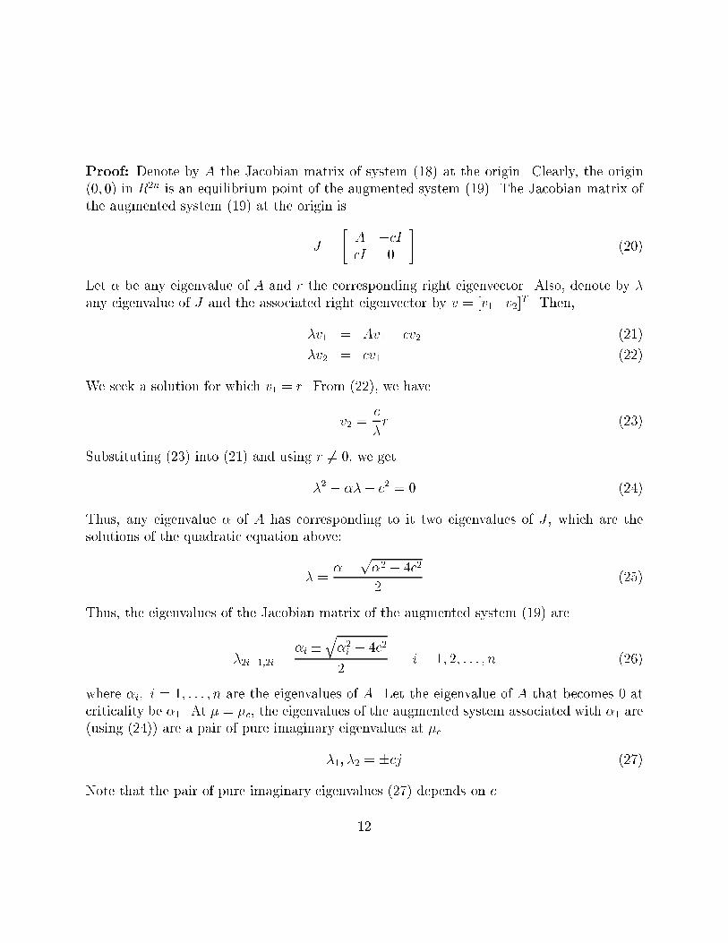
Proof: Denote by A the Jacobian matrix of system (18) at the origin. Clearly, the origin(0; 0) in R2n is an equilibrium point of the augmented system (19). The Jacobian matrix ofthe augmented system (19) at the origin is
J =
"A �cIcI 0
#(20)
Let � be any eigenvalue of A and r the corresponding right eigenvector. Also, denote by �any eigenvalue of J and the associated right eigenvector by v = [v1 v2]
T . Then,
�v1 = Av1 � cv2 (21)
�v2 = cv1 (22)
We seek a solution for which v1 = r. From (22), we have
v2 =c
�r (23)
Substituting (23) into (21) and using r 6= 0, we get
�2 � ��+ c2 = 0 (24)
Thus, any eigenvalue � of A has corresponding to it two eigenvalues of J , which are thesolutions of the quadratic equation above:
� =��p
�2 � 4c2
2(25)
Thus, the eigenvalues of the Jacobian matrix of the augmented system (19) are
�2i�1;2i =�i �
q�2i � 4c2
2i = 1; 2; : : : ; n (26)
where �i; i = 1; : : : ; n are the eigenvalues of A. Let the eigenvalue of A that becomes 0 atcriticality be �1. At � = �c, the eigenvalues of the augmented system associated with �1 are(using (24)) are a pair of pure imaginary eigenvalues at �c
�1; �2 = �cj (27)
Note that the pair of pure imaginary eigenvalues (27) depends on c.
12
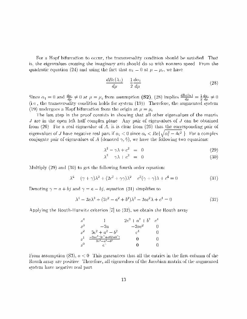
For a Hopf bifurcation to occur, the transversality condition should be satis�ed. Thatis, the eigenvalues crossing the imaginary axis should do so with nonzero speed. From thequadratic equation (24) and using the fact that �1 = 0 at � = �c, we have
dRe(�1)
d�=
1
2
d�1
d�(28)
Since �1 = 0 and d�1d�
6= 0 at � = �c from assumption (S2), (28) implies dRe(�1)d�
= 12d�1d�
6= 0
(i.e., the transversality condition holds for system (19)). Therefore, the augmented system(19) undergoes a Hopf bifurcation from the origin at � = �c.
The last step in the proof consists in showing that all other eigenvalues of the matrixJ are in the open left half complex plane. Any pair of eigenvalues of J can be obtainedfrom (26). For a real eigenvalue of A, it is clear from (26) that the corresponding pair of
eigenvalues of J have negative real part if �i < 0 since �i < Refq�2i � 4c2 g. For a complex
conjugate pair of eigenvalues of A (denoted ; � ), we have the following two equations:
�2 � � + c2 = 0 (29)
�2 � � � + c2 = 0 (30)
Multiply (29) and (30) to get the following fourth order equation:
�4 � ( + � )�3 + (2c2 + � )�2 � c2( + � )�+ c4 = 0 (31)
Denoting = a+ bj and � = a� bj, equation (31) simpli�es to
�4 � 2a�3 + (2c2 + a2 + b2)�2 � 2ac2�+ c4 = 0 (32)
Applying the Routh-Hurwitz criterion [7] to (32), we obtain the Routh array
s4 1 2c2 + a2 + b2 c4
s3 �2a �2ac2 0s2 3c2 + a2 + b2 c4 0
s1 �2ac2(2c2+a62+b2)3c2+a2+b2
0 0
s0 c4 0 0
From assumption (S3), a < 0. This guarantees that all the entries in the �rst column of theRouth array are positive. Therefore, all eigenvalues of the Jacobian matrix of the augmentedsystem have negative real part.
13
From the foregoing discussion, it is also clear that if any eigenvalue of A has positivereal part, then the corresponding eigenvalues of J also have positive real part. This provesthat if the origin is unstable for the plant, then it is also unstable for the augmented system.
Note that since the value c in equation (19) is adjustable, we can control the crossingfrequency of the complex conjugate pair of eigenvalues of the augmented system. Thus,for detecting stationary bifurcation, we only need to monitor a frequency band around thechosen value of c. It is also possible to slowly vary c in a controlled fashion, giving addedcon�dence in our assessment that an instability is imminent.
There are some other advantages of our monitoring system. The augmented system (19)has the same critical parameter value (�c) as the original system. This is actually not aluxury but a necessity for the system to be practically useful. In addition, the �nal partof the proof shows that augmenting the states yi and applying the feedbacks cyi to theoriginal system does not change the local stability of the system. Moreover, to apply themonitoring system, we do not need knowledge of the original system. However, there aresome restrictions and further considerations in applying the suggested monitoring system togeneral physical systems. We will discuss these in subsequent sections.
We assumed above that the stationary bifurcation was such that the transversality con-dition is satis�ed. This means that the eigenvalue that vanishes at criticality must crossinto the right half of the complex plane with nonzero speed as the parameter is varied. In asaddle node bifurcation, however, the nominal equilibrium disappears at criticality, so thatthe transversality condition does not hold. For a saddle-node bifurcation, the augmentedsystem of this section results in a degenerate Hopf bifurcation. The possible bifurcationdiagrams for degenerate Hopf bifurcation are more complex than for Hopf bifurcation [16],[10]. However, for the purpose of detecting incipient instability, the details of the ensuing bi-furcation are not important. These details become important when we consider the system'spost-bifurcation behavior.
3.2 Detecting Hopf Bifurcation using Monitoring System
In this section, we consider the e�ect of the monitoring system of the proceeding section ona system that undergoes Hopf bifurcation instead of stationary bifurcation. Consider againthe system (18), repeated here for convenience:
_x = f(x; �) (33)
14

(H1) The origin is an equilibrium point of (33) for all values of �.
(H2) System (33) undergoes a Hopf bifurcation from the origin at � = �c.
(H3) All other eigenvalues of Df(0; �c) are in the open left half complex plane.
As in the foregoing section, let the augmented system (plant plus monitoring system) be
_xi = fi(x; �)� cyi
_yi = cxi (34)
where x 2 Rn, y 2 Rn, c 2 R, and i = 1; 2; : : : ; n.
Proposition 2 Under the assumptions (H1)-(H3), the augmented system (34) undergoes acodimension two bifurcation at � = �c, in which two complex conjugate pairs of eigenvaluescross the imaginary axis. Moreover, for any value of � if the origin of the original system isasymptotically stable (resp. unstable), then the origin is asymptotically stable (resp. unstable)for the augmented system.
Proof: First, we show that the augmented system has two pairs of pure imaginary eigenval-ues at the origin for � = �c, and that these eigenvalues satisfy the transversality condition.
From assumption (H2), the Jacobian matrix of the original system at the origin has apair of pure imaginary conjugate eigenvalues (denote them by j!;�j!) for � = �c. From theproof of Proposition 1, it is clear that each of these eigenvalues results in a pair of eigenvaluesfor the augmented system which are the solutions of the following equations:
�2 � j!�+ c2 = 0 (35)
�2 + j!�+ c2 = 0 (36)
By multiplying the equations above, we get a fourth order equation the solutions of whichare eigenvalues of augmented system:
�4 + (2c2 + !2)�2 + c4 = 0 (37)
The four solutions of the equation above are given by
� = �q�2c2 � !2 �p
4c2!2 + !4
p2
(38)
15

Note that 2c2 + !2 >p4c2!2 + !4 for all c; ! 2 R. Therefore, the Jacobian matrix of
the augmented system has two pairs of pure imaginary conjugate eigenvalues at the criticalparameter value.
To check the transversality condition, consider the eigenvalues for � near �c. Near � = �c,we have the following fourth order equation the solutions of which result from the pair ofcomplex conjugate eigenvalues (�� !j) of the original system (see (31)):
�4 � 2��3 + (2c2 + �2 + !2)�2 � 2c2� + c4 = 0 (39)
Since � is close to �c, by continuity it follows that this equation has two pairs of complexconjugate eigenvalues as its solutions for � near �c. Denote these as e� fj; g�hj. The nextrelationship is now easily demonstrated:
�2� =4X
i=1
�i = e+ g (40)
�2c2� =4X
i;j;k=1
i6=j 6=k
�i�j�k = 2g(e2 + f 2) + 2e(g2 + h2) (41)
where �i; �j; �k are roots of (39). Taking the derivative of both sides of the equation abovewith respect to � and evaluating at � = �c (e = g = 0, � = 0, 2 = c� a) gives
de
d�+dg
d�= �2d�
d�
h2de
d�+ f 2 dg
d�= �c2d�
d�(42)
Next we solve Eq. (42) for dg
d�; ded�. Also, h and f are not 0 at the critical point from (38)
and f 6= h at the critical point if c 6= 0. These conditions guarantee that if d�d�6= 0, then
dg
d�6= 0; de
d�6= 0.
The last step in the proof consists in showing that all other eigenvalues of the Jacobianmatrix J of (34) lie in the open left half complex plane. Note that we have the same formof matrix J as in the proof of Proposition 1:
J =
"A �cIcI 0
#(43)
where all noncritical eigenvalues of A have negative real part. We can use the same procedureas in Proposition 1 to prove that if all noncritical eigenvalues of A have negative real part,then all corresponding eigenvalues of J have negative real part.
16

It is also clear that if any eigenvalue of A has positive real part, then the correspondingeigenvalues of J also have positive real part. This implies that if the original system isunstable, then the augmented system is also unstable.
Since two pairs of eigenvalues of the augmented system cross the imaginary axis at thecritical parameter value, we can expect to see two peaks in the power spectrum as the systemnears the bifurcation point. From (38), we see that the values of the pairs of imaginaryeigenvalues at criticality depend on c. Hence, we can change the location of the powerspectrum peaks by changing c. Moreover, we can predict the exact locations of the peaks ifthe pair of eigenvalues crossing the imaginary axis in the original system is known.
Because two pairs of eigenvalues cross the imaginary axis for the augmented system, theaugmented system undergoes a codimension two bifurcation. The nature of the bifurcationbehavior depends strongly on f(x; �). The possible bifurcation diagrams for the associateddegenerate Hopf bifurcation can be found in [16], [10]. However, as was the case for de-tecting incipient stationary bifurcation, the details of the degenerate Hopf bifurcation arenot important. They become important when we consider the system's post-bifurcationbehavior.
4 Stabilization of Bifurcated Limit Cycle
in the Augmented System
In this section, we suppose that the plant is subject to loss of stability through a stationarybifurcation. In these circumstances, the monitoring system proposed above results in a Hopfbifurcation in the augmented system. Besides being able to predict that a bifurcation isabout to take place, it would be useful if the monitoring system could also ensure stabilityof the bifurcated solution. That is, a system that can perform both monitoring and controlfunctions is desirable. The purpose of this section is to illustrate how the monitoring systemwe have proposed can be modi�ed to serve in both capacities. Liberal use is made of thebifurcation formulas and associated results summarized in Appendix B.
4.1 Stability of the Bifurcated Limit Cycle
of the Augmented System
First, we consider the relationship between the stability of bifurcated equilibrium points ofthe original system and stability of the bifurcated limit cycle of the augmented system. If
17
stability of the bifurcated equilibria of the original system implies stability of the bifurcatedperiodic solution of the augmented system, then bifurcation control design need only beperformed for the original system. We proceed to show, however, that the stability propertiesof the bifurcation persist in the case of scalar systems, but not generally for systems ofdimension two or higher.
Let the plant be given by_x = f(x; �) (44)
where x 2 Rn is the state vector and � 2 R is the bifurcation parameter, and the noise inputis neglected for the purposes of this section. Suppose that at the critical parameter value� = �c, the Jacobian matrix of (44) evaluated at the equilibrium point x0 = 0 has one zeroeigenvalue.
For simplicity, we �rst consider the one-dimensional case (n = 1), i.e., suppose thestate vector of (44) is a single variable. Also, suppose system (44) undergoes a pitchforkbifurcation. It is easy to see that the left (l) and right (r) eigenvectors corresponding tothe simple zero eigenvalue at criticality can be taken as any nonzero constants. Set r = 1and l = 1, so that r and l satisfy the normalization lr = 1. Lemma 1 (see Appendix B)then applies directly, allowing calculation of the associated bifurcation stability coe�cients�1 and �2. As discussed in Appendix B, the pitchfork bifurcation is supercritical (givingstable bifurcated equilibria) if �1 = 0 and �2 < 0. Since system (44) is assumed to undergoa pitchfork bifurcation, �1 = 0:
�1 = lQ(r; r) =@2f
@x2(0) = 0 (45)
Thus, Q(r; r) vanishes. Since Q(r; r) = 0, we have x2 = 0 (using the notation of AppendixB). Thus, �2 becomes
�2 = 2lC0(r; r; r) =2
3!
@3f
@x3(0) (46)
The augmented system corresponding to the plant (44) is
_x = f(x; �)� cy
_y = cx (47)
where x; y; � 2 R. We have shown that the augmented system undergoes a Hopf bifurcation ifthe original system undergoes a pitchfork bifurcation. To check the stability of the bifurcatedperiodic solution of (47), we only have to check the sign of the Hopf bifurcation stability
18

coe�cient �2 (102). At criticality, the Jacobian matrix of (47) is
L0 :=
"0 �cc 0
#(48)
The matrix L0 has an eigenvalue cj with corresponding right eigenvector r =h1 �j
iTand
left eigenvector l = 12
h1 j
i. Eigenvalue �cj has right eigenvector �r and left eigenvector �l.
Note that higher order terms only come from f(x; �) and they are not a function of y. Fromthis observation, we have
Q((x; y); (x; y)) =
0B@ 1
2!
hx y
i " @2f
@x2(0) 0
0 0
# "x
y
#
0
1CA
=
12@2f
@x2(0)x2
0
!(49)
From equation (45), equation (49) implies that Q(r; �r) and Q(r; r) both vanish. Therefore,the solutions of (100) and (101) are a = 0 and b = 0. Now, �2 of (47) becomes
�2 = 2Ref34lC(r; r; �r)g = 2
3
4
1
3!
@2f
@x3(0) (50)
since higher order terms only come from f(x; �) and none depend on y.Note that the sign of (46) agrees with the sign of (50). The next proposition therefore
follows.
Proposition 3 Suppose the system (44) is of �rst order, i.e., n=1. If the plant (44) un-dergoes a supercritical pitchfork bifurcation (respectively a subcritical pitchfork bifurcation),then the transformed system (47) undergoes a supercritical Hopf bifurcation (respectively asubcritical Hopf bifurcation).
Next, we consider the case n � 2, that is, the case in which the dimension of the plantis at least 2. We show using an example that the monitoring system proposed above doesnot necessarily preserve the stability character of the bifurcation in the plant. That is, asupercritical pitchfork bifurcation (resp. a subcritical pitchfork bifurcation) in the plantneed not result in a supercritical Hopf bifurcation (resp. a subcritical Hopf bifurcation) inthe augmented system.
19

Consider the example
_x1 = ��x1 � x31 + x1x2
_x2 = �x2 + kx21 (51)
where � 2 R is a bifurcation parameter and k 2 R is a constant. It is easy to see that theorigin is an equilibrium point for all parameter values � and that a pitchfork bifurcationoccurs for � = 0. Moreover, a simple calculation shows that �2 for this pitchfork bifurcationis �1. This implies that system (51) undergoes a supercritical pitchfork bifurcation at � = 0.
The augmented system corresponding to (51) is
_x1 = ��x1 � x31 + x1x2 � cy1
_y1 = cx1
_x2 = �x2 + kx21 � cy2
_y2 = cx2 (52)
As discussed in Appendix B, typically a Hopf bifurcation's stability is determined by a singlebifurcation stability coe�cient �2 (this di�ers from the �2 coe�cient in the study of pitchforkbifurcations). The Hopf bifurcation is supercritical if the coe�cient �2 is negative, and it issubcritical if the coe�cient is positive. We now calculate �2 for the Hopf bifurcation thatoccurs in the augmented system (52). To facilitate application of the formulas in AppendixB, denote the state vector of (52) as z = (z1; z2; z3; z4)
T where z1 := x1, z2 := y1, z3 := x2,and z4 := y2. The Jacobian matrix of (52) evaluated at the origin at criticality is
266640 �c 0 0c 0 0 00 0 �1 �c0 0 c 0
37775 (53)
One eigenvalue of this matrix is cj, and it has corresponding right eigenvector r =h1 �j 0 0
iTand left eigenvector l = 1
2
h1 j 0 0
i. The conjugate eigenvalue �cj has right eigenvector
�r and left eigenvector �l. The Taylor series expansion of the right side of (52) has the followingquadratic and cubic terms:
Q(z; z) =
26664z1z30kz210
37775 =
26664x1x20kx210
37775
20

C(z; z; z) =
26664�z31000
37775 =
26664�x31000
37775 (54)
Therefore, we have
Q(r; �r) = Q(r; r) =
2666400k
0
37775
C(r; r; �r) =
26664�1000
37775 (55)
Solving Eqs. (100) and (101) of Appendix B, we obtain
a =h0 0 0 �k
c
iTb =
h0 0 kj
2j�3ck
2j�3c
iT(56)
Substituting these values in (102) of Appendix B, we �nd that �2 for system (52) is
�2 = �3
4+
k
4 + 9c2(57)
Note that for su�ciently large k, �2 is positive. For such values of k, the augmented system(52) therefore undergoes a subcritical Hopf bifurcation even though the plant undergoes asupercritical pitchfork bifurcation. Thus, for n � 2, the monitoring system as presentedabove does not necessarily preserve the stability of bifurcated solutions. We now proceed tomodify the design to address this de�ciency.
4.2 Redesign for Combined Monitoring
and Bifurcation Stabilization
In this section, we modify our monitoring system such that the bifurcated limit cycle occur-ring in the augmented system is guaranteed stable regardless of the stability of the pitchfork
21

bifurcation occurring in the plant. That is, we ensure that the Hopf bifurcation in theaugmented system is supercritical, and that this holds regardless of whether the pitchforkbifurcation in the original system is supercritical or subcritical. The modi�cation that weintroduce in the monitoring system involves the addition of a nonlinear term with a gainparameter that can be tuned to ensure the desired result.
Let the plant obey the dynamics
_x = f(x; �); (58)
which we assume undergoes a pitchfork bifurcation from the origin for � = �c. Here, x 2 Rn
and � 2 R is the bifurcation parameter. Denote by rs and ls the right and left eigenvectors,respectively, corresponding to the simple zero eigenvalue of the system linearization at � =�c. Take the �rst component of rs to be 1 and impose the normalization lsrs = 1 (followingthe procedure in Appendix B).
Now consider the following redesign of the augmented system:
_xi = fi(x; �)� cyi
_yi = cxi �mx21yi (59)
Here, c and m are real constants. At criticality, the system (59) has Jacobian matrix
J =
"A �cIcI 0
#(60)
at the origin, written in terms of A, the Jacobian matrix of (58). Employing Proposition 1,it is easy to show that the augmented system (59) undergoes Hopf bifurcation and that thematrix J has eigenvalues �ci. Moreover, the right and left eigenvectors of J correspondingto the eigenvalue cj are given by
r =hrs �jrs
iTl =
1
2
hls jls
i(61)
Also, the right and left eigenvectors corresponding to the eigenvalue �cj are given by �r and�l, respectively.
The stability of the bifurcated periodic solution of the augmented system is determinedby the sign of the bifurcation stability coe�cient �2 (Eq. (102), Appendix B):
�2 = 2Ref2lQ0(r; a) + lQ0(�r; b) +3
4lC(r; r; �r)g (62)
22

Since there are no quadratic terms in yi in the augmented system (59), �2 simpli�es to
�2 = 2Ref2lsQf (r; a) + lsQf (�r; b) +3
4lC(r; r; �r)g (63)
where Qf (�; �) denotes the quadratic terms in the Taylor expansion of f(x; �c). Moreover,we can simplify
lC(r; r; �r) = lsCf(r; r; �r) +j
2lsCy(r; r; �r)
= lsCf(r; r; �r) +m
6
nXi=1
lisris(r
1s)
2 (64)
where Cf(x; x; x) denotes the cubic terms in the Taylor expansion of f(x; �c), and ris and l
is
denote the i-th component of rs and ls, respectively. Since the �rst component of r1s is 1 andlsrs = 1, (64) reduces to
lC(r; r; �r) = lsCf(r; r; �r)� m
6(65)
Hence, �2 becomes
�2 = 2Ref2lsQf (r; a) + lsQf(�r; b) +3
4lsCf(r; r; �r)g � 3m
12(66)
By choosing m positive and su�ciently large, we can ensure that �2 will be negative. Thiswill imply that the Hopf bifurcation occurring in the augmented system (59) is supercritical.
Here, we have suggested only one of many possible designs that render the Hopf bifurcatedsupercritical. The method is robust, since the e�cacy of the design does not depend on thedetails of the plant model. For any given plant, a su�ciently large feedback gain m willresult in supercriticality of the Hopf bifurcation. Note that we added a nonlinear term onlyto the dynamics of the augmented states yi not to those of the physical system states xi. Wetherefore have considerable freedom in choosing the nonlinear feedback gain m.
5 Reduced Order Monitoring System
The closed-loop monitoring systems introduced in the preceding two sections entail the useof full state feedback. In this section, we alleviate this requirement for plant models thatcan be viewed as singularly perturbed (or two time-scale) systems. We design a monitoringsystem in which only the slow states are fed back to the controls.
23

Consider a plant given by a singularly perturbed system of the form
_x = f(x; z; �; �)
� _z = g(x; z; �; �) (67)
where x 2 Rn, z 2 Rm, �; � 2 R and � is small but positive. The reduced system is obtainedby formally setting � = 0 in (67), giving
_x = f(x; z; �; 0)
0 = g(x; z; �; 0) (68)
Let m0 = (0; z0) be an equilibrium point of the reduced system. Also, assume
(SP1) m0 = (0; z0) is an equilibrium point of (68) for all values of �.
(SP2) f; g; are Cr(r � 5) in x; z; �; � in a neighborhood of (m0; 0; 0).
(SP3) No eigenvalue of D2g(0; z0; 0; 0) has zero real part.
(SP4) The reduced system undergoes a stationary bifurcation at m0 for the critical parametervalue � = �c.
Let the augmented system (plant plus monitoring system) corresponding to (67) be
_x = f(x; z; �; �)� cy
_y = cx
� _z = g(x; z; �; �) (69)
Proposition 4 Let (SP1)-(SP4) above hold. Then there is an �0 > 0 and for each � 2 [0; �0]
the augmented system (69) undergoes a Hopf bifurcation at an equilibrium m��c;�
0 near m0 fora critical parameter value ��c near �c.
Proof: By virtue of Theorem in [1] on persistence of Hopf bifurcation under singular pertur-bation, we need to verify two conditions. The �rst is that the reduced system correspondingto (69) undergoes a Hopf bifurcation at (0; 0; z0) at the critical parameter value � = �c. Thesecond condition is that the Jacobian matrix of g with respect to the fast variables z doesnot possess any eigenvalues with zero real part. The reduced system
_x = f(x; z; �; 0)� cy
_y = cx
0 = g(x; z; �; 0) (70)
24

Since the original reduced system (68) undergoes a stationary bifurcation, we can applyProposition 1 to (70) to show that the reduced augmented system (70) undergoes Hopf bi-furcation at the critical parameter value � = �c. The result now follows from [1].
Proposition 4 is useful because it implies that we only have to augment and feed back slowstates in a two-time scale system to transform stationary bifurcation into Hopf bifurcation.
6 Monitoring System for Nonzero Equilibrium Point
Although the results of the preceding sections do not depend on availability of an accuratemodel of the plant, they do require knowledge of the nominal equilibrium. In this section, wealleviate this requirement through a re-design of the monitoring system. Not surprisingly,the increased generality comes with some cost, mainly in the simplicity of the observedinstability precursor.
The requirement of a known equilibrium is embodied in assumption (S1), which statesthat the nominal equilibrium point of the plant is �xed at the origin for all parameter values.Through a simple parameter-dependent coordinate change, it is clear that the results of thepreceding sections still apply under the milder assumption that the equilibrium is a knownfunction of the parameter.
Assumption (S1) was invoked so that the equilibrium point of the plant is not changedupon applying state feedback. A standard control technique for exactly preserving an equi-librium despite model uncertainty involves the use of washout �lters [15]. Our revised designsin this section entail adjoining a washout �lter to the previous monitoring system designs.
Denote by x0(�) the nominal equilibrium point of system (18). We now allow the equi-librium to depend in some unknown fashion on the parameter �.
The following re-designed augmented system involves two sets of additional variables:the vector y, which appears in the original design (19); and the vector z, the washout �lterstates:
_xi = fi(x; �)� cyi
_yi = cxi + azi
_zi = yi (71)
for i = 1; 2; : : : ; n, where a; c 2 R.Proposition 5 Assume the original system (18) satis�es (S2) and (S3) at an equilibriumpoint x0(�) not necessarily at the origin. Then the augmented system (71) undergoes a
25

codimension 2 bifurcation at � = �c. At criticality, the linearization of (71) possesses onesimple zero eigenvalue and a pair of pure imaginary eigenvalues.
Proof: The equilibrium point of the augmented system (71) is (x0; 0; z0), where z0 is solutionof cxi+azi = 0. Note that new augmented system keeps x0 as a component of this equilibriumpoint. The Jacobian matrix of (71) evaluated at this equilibrium point is
J =
264 A �cI 0cI 0 aI
0 I 0
375 (72)
where A is the Jacobian matrix of the original system evaluated at x0. Let � be any eigen-value of A and r corresponding eigenvector. Also, assume � is an eigenvalue of J witheigenvector v = [vT1 vT2 vT3 ]
T . Then
�v1 = Av1 � cv2 (73)
�v2 = cv1 + av3 (74)
�v3 = v2 (75)
Attempt a solution v for which v1 = r. Solve (74) and (75) for v2 and v3 in terms of r, weget
v2 =c�
�2 � ar
v3 =c
�2 � ar
Substituting the equation for v2 into (73) and using r 6= 0, gives
�3 � ��2 + (c2 � a)�+ a� = 0 (76)
Since one eigenvalue of A becomes 0 at � = �c, we can set � = 0 to get following equationfor the expected pair of eigenvalues system at criticality:
�3 + (c2 � a)� = 0 (77)
If we choose a < 0, then J has eigenvalues 0;�pc2 � a j which correspond to the zeroeigenvalue of the original system criticality.
26

Next, we check the transversality condition. Equation (76) which corresponds to crossingsimple real eigenvalue of original system has one real and a pair of complex conjugate asits solution near the critical point. Denote � as the real eigenvalue and � � j as thepair of complex conjugate eigenvalue. Solving this notation in (76) and separating real andimaginary parts, we obtain
� + 2 � � = ���(�2 + 2) = �a (78)
Di�erentiating these equations with respect to �, gives
d�
d�+ 2
d�
d�= �d�
d�
d�
d�(�2 + 2) + 2
d�
d��� + 2
d
d� � =
d�
d�a (79)
At the critical parameter value � = �c, � = 0, � = 0, and 2 = c2 � a. Thus, at � = �c,
d�
d�+ 2
d�
d�= �d�
d�(80)
d�
d�(c2 � a) =
d�
d�a (81)
From equation (81), d�d�6= 0. Solving these equations for d�
d�, gives
d�
d�= �1
2
c
c2 � a
d�
d�(82)
which is nonzero if d�d�6= 0 and a < 0.
As was the case with Proposition 1, the �nal step in the proof consists of showing thatall other eigenvalues of the matrix J are in the open left half complex plane (C�). There arethree eigenvalues of J which correspond to one negative real value eigenvalue of A and theseeigenvalues are solutions of the (76). By using the Routh-Hurwitz criterion, we can showthat solutions of equation (76) in C� if the corresponding real eigenvalue of A is in C�. Forthe complex conjugate pair of eigenvalues of A ( ; � ), we have following two equations
�3 � �2 + (c2 � a)�+ a = 0 (83)
�3 � � �2 + (c2 � a)�+ a� = 0 (84)
27

Multiply (83) and (84) to get the sixth order equation
�6 � ( + � )�5 + (2(c2 � a) + � )�4 + ( + � )(2a� c2)�3
+ ((c2 � a)2 � 2a � )�2 + (c2 � a)a( + � )�+ a2 � = 0 (85)
By applying the Routh-Hurwitz criterion to (85), we can show that all solutions of (85) arein the open left half complex plane if Re( ) is negative (details are in Appendix A).
We have proved that the new augmented system (71) with nominal equilibrium notnecessarily at the origin replaces a stationary bifurcation with a codimension two bifurcation.Note that the design gives the same critical parameter value for the plant and the augmentedsystem. In addition, the crossing eigenvalues at critical point are located 0 and �pc2 � a j.Also, note that an original simple zero eigenvalue persists under the augmentation. Thus, themonitoring system's e�ectiveness has to do with its introduction of a purely imaginary pairof eigenvalues at criticality in addition to the zero eigenvalue. Near bifurcation, we expectpower spectrum peaks to be located at 0 and
pc2 � a. By varying c and a (both tunable
parameters), we can tune the location of the peak atpc2 � a as desired. This exibility
increases our assurance that the power spectrum peak is caused by closeness to instabilityrather than by other factors (such as noise). However, the new augmented system (71) alsocomes with some disadvantages compared to the system in Proposition 1. In Proposition 1,we transform a stationary bifurcation into a Hopf bifurcation. In other words, the systemhas a limit cycle as its solution instead of a new equilibrium point near of bifurcation. Incomparison to the previous augmented system design (19), the new augmented system (71)shows more complicated bifurcation behavior [9]. The system is no longer guaranteed to havea periodic orbit as a solution near bifurcation. Either a periodic orbit or a new equilibriumpoint could result at bifurcation. The bifurcation diagram depends strongly on the vector�eld f(x; �). However, it may be possible that augmented system has desired bifurcationdiagram by introducing some nonlinear terms into augmented states. Of course, to do thatwe have detail knowledge on f(x; �). Details on codimension two bifurcations can be foundin [9]. However, for the purpose of monitoring, it is enough to have a discernible powerspectrum peak when the system approaches instability.
The next proposition asserts that the new augmented system also works for singularlyperturbed systems using fewer states for feedback. The only di�erence from the previousresults on singularly perturbed systems is that we no longer require (SP1) of Section 5.Using the same notation as in Section 5, we have the following proposition.
Proposition 6 Let (SP2)-(SP4) of Section 5 hold for the system (18). Then there is an�0 > 0 and for each �0 2 [0; �0] the following extended system undergoes a codimension two
28

(one real and a pair of complex eigenvalues crossing) bifurcation at an equilibrium m��c;�
0 nearm0 for a critical parameter value ��c near �c:
_xi = fi(x; z; �; �)� cyi
_yi = cxi + awi
_wi = yi
� _z = g(x; z; �; �) (86)
where i = 1; 2; : : : ; n.
Proof: Follows directly from Proposition 5 and Theorem 7 of [1].
7 An Example
Consider again the simple system (51) which undergoes a pitchfork bifurcation. For conve-nience, we rewrite the equations for the plant (including a noise term) augmented with amonitoring system:
_x1 = ��x1 � x31 + x1x2 � cy1 +N(t)
_y1 = cx1
_x2 = �x2 + 5x21 � cy2
_y2 = cx2 (87)
Here, N(t) is a white Gaussian noise. The system (87) undergoes a Hopf bifurcation at� = 0, which is the parameter value where a pitchfork bifurcation occurs for the originalsystem (51). The origin loses stability as � is decreased through � = 0.
The simulation results in this section were obtained by the MATLAB Simulink package.Figure 3 shows the location of the power spectrum peak in frequency as the parameter cis (quasistatically) changed. The simulations were done for a parameter value of � = 0:1,which is before the origin loses stability. Note from the �gure that the location of the powerspectrum peak obtained from simulation (shown as an asterisk in Figure 3) agrees well withthe predicted location (straight line in Figure 3).
8 Conclusions
We have proposed closed-loop monitoring systems for detection of incipient instability inuncertain nonlinear plants. These systems make use of characteristics of the power spectrum
29

01
23
45
67
89
100 2 4 6 8 10 12
c
Location of power spetcrum peak (rad/sec)
Figu
re3:
Variation
oflocation
ofpow
erspectru
mpeak
with
c(�
=0:1)
30

of a measured output in the vicinity of an instability. By employing closed-loop designs, weare able to more reliably monitor for incipient instability through on-line tuning of controlparameters. Two time-scale models were used to reduce the number of measurements fedback in the closed-loop monitoring system. We have studied the impact of the monitoringsystems on stability of bifurcations that occur when stability is lost, and proposed designmodi�cations to ensure stability of bifurcated solutions in a robust fashion.
A Routh-Hurwitz Calculation for
Proposition 5
Using the same notation as in Proposition 5, and letting = � + j! and � = � � j!, Eq.(85) becomes
�6 � 2��5 + (2(c2 � a) + �2 + !2)�4 + 2�(2a� c2)�3 +
((c2 � a)2 � 2a(�2 + !2))�2 + 2(c2 � a)a��+ a2(�2 + !2) = 0
Applying the Routh-Hurwitz criterion to the equation above, we obtain the Routh array
s6 1 2(c� a) + � (c� a)2 � 2a(�2 + !2) a2(�2 + !2)
s5 �2� 2�(2a� c) 2�a(c� a) 0
s4 c+ �2 + !2 c2 � ac� 2a(�2 + !2) a2(�2 + !2) 0
s32�c(a�(�2+!2))
c+�2+!22�ac(c�a+�2+!2)
c+�2+!20 0
s2 � a2(�2 + !2) 0 0
s1�2ac3�(c+�2+!2)a(�2+!2+c)�(a+c)2
0 0 0
s0 a2(�2 + !2) 0 0 0
where � = a(�2+!2)(c+�2+!2)�(a+c)2(�2+!2)a�(�2+!2)
. If a < 0 and � < 0, then all entries in the �rst
column of this array are positive. Therefore, under this condition all solutions of (85) havenegative real part.
B Stability of Bifurcated Solutions
In this appendix, we recall formulas for determining the local stability of bifurcated solutions.Details can be found in Abed and Fu [2],[3].
31
Consider a one-parameter family of nonlinear autonomous systems
_x = f(x; �) (88)
where x 2 Rn is the vector state and � is a real-valued parameter. Let f(x; �) be su�cientlysmooth in x and � and let x0;� be the nominal equilibrium point of the system as a functionof the parameter �.
First, we consider the case of stationary bifurcation. For simplicity, we take the criticalparameter value to be �c = 0 in the statement of the next hypothesis.
(S) The Jacobian matrix of system (88) at the equilibrium x0;� has a simple zero eigenvalue�1(�) with �01(0) 6= 0, and the remaining eigenvalues lie in the open left half of thecomplex plane for � = 0.
The Stationary Bifurcation Theorem asserts that hypothesis (S) implies a stationarybifurcation from x0;� at � = 0 for (88). A new equilibrium branch bifurcates from x0;� at� = 0. The theorem states that near the point (x0;0; 0) of the (n + 1)-dimensional (x; �)-space, there exists a locally unique curve of critical points (x(�); �(�)), distinct from x0;� andpassing through (x0;0; 0), such that for all su�ciently small j�j, x(�) is an equilibrium pointof (88) when � = �(�). (Here, � is an auxiliary small parameter.)
The series expansions of x(�); �(�) can be written as
�(�) = �1� + �2�2 + � � � (89)
x(�) = x0;� + x1� + x2�2 + � � � (90)
If �1 6= 0, the system undergoes a transcritical bifurcation from x0;� at � = 0. That is,there is a second equilibrium point besides x0;� for both positive and negative values of �with j�j small. If �1 = 0 and �2 6= 0, the system undergoes a pitchfork bifurcation for j�jsu�ciently small. That is, there are two new equilibrium points existing simultaneously,either for positive or for negative values of � with j�j small. The new equilibrium pointshave an eigenvalue �(�) which vanishes at � = 0. The series expansion �(�) is given by
�(�) = �1� + �2�2 + � � � (91)
We have the exchange of stability formula:
�1 = ��1�0(0) (92)
Moreover, in case �1 = 0, �2 is given by
�2 = �2�2�0(0) (93)
32

Eqs. (92),(93) are not explicit formulas for �1 and �2. Explicit formulas are given Lemma 1.The bifurcation stability coe�cients �1 and �2 can be obtained using eigenvector com-
putations and series expansion of the vector �eld. System (88) can be written in the seriesform
_~x = L�~x+Q�(~x; ~x) + C�(~x; ~x; ~x) + � � �= L0~x + �L1~x+ �2L2~x + � � �
+Q0(~x; ~x) + �Q1(~x; ~x) + � � �+C0(~x; ~x; ~x) + � � � (94)
where ~x = x � x0;0; L�; L1; L2 are n � n matrices, Q�(x; x); Q0(x; x); Q1(x; x) are vector-valued quadratic forms generated by symmetric bilinear forms, and C�(x; x; x); C0(x; x; x)are vector-valued cubic forms generated by symmetric trilinear forms.
By assumption, the Jacobian matrix L0 has a simple zero eigenvalue with the remain-ing eigenvalues stable. Denote by l and r the left (row) and right (column) eigenvectors,respectively, of the matrix L0 associated with the simple zero eigenvalue, where the �rstcomponent of r is set to 1 and the left eigenvector l is chosen such that lr = 1. (Settingthe �rst component of r to 1 sometimes requires a re-ordering of the state variables.) Thefollowing well known fact is used in the statement of the next lemma:
�0(0) = lL1r (95)
The two lemmas that follow give stability criteria for the bifurcated equilibria of system(94). The �rst addresses to pitchfork bifurcation, while the second addresses transcriticalbifurcation.
Lemma 1 Let hypothesis (S) hold. Then
�1 = lQ0(r; r) (96)
Also, if �1 = 0, then�2 = 2lf2Q0(r; x2) + C0(r; r; r)g (97)
where x2 solvesL0x2 = �Q0(r; r) (98)
The bifurcated equilibrium points of (94) near x0� for � near 0 are asymptotically stable if�1 = 0 and �2 < 0, but they are unstable if �1 = 0 and �2 > 0.
33

Lemma 2 Let hypothesis (S) hold, and suppose that �1 6= 0 (this can be checked using (96)).Then the bifurcated solution is asymptotically stable on one side of � = 0 and is unstable onthe other. For any given value of � near 0, the stability of the bifurcated solution is oppositethat of the nominal equilibrium.
Now consider system (88) under for the following hypothesis, which implies occurrence ofHopf bifurcation. Again, for simplicity the critical value of the parameter is taken as �c = 0.
(H) The Jacobian matrix of system (88) at the equilibrium x0;�=0 has a pair of pure imag-inary eigenvalues �1(0) = j!c and ��1(0) = �j!c with !c 6= 0, the transversality
condition @Re[�(0)]@�
6= 0 is satis�ed, and all the remaining eigenvalues lie in the open lefthalf complex plane.
Under these conditions, the Hopf Bifurcation Theorem asserts the existence of a one-parameter family p�; 0 < � � �0 of nonconstant periodic solutions of system (88) emergingfrom x = x0;� at the parameter value 0 for su�ciently small j�j. Exactly one of the charac-teristic exponents of p� governs the asymptotic stability and is given by a real, smooth andeven function
�(�) = �2�2 + �4�
4 + � � � (99)
Speci�cally, p� is orbitally stable if �(�) < 0 but is unstable if �(�) > 0. Generically the localstability of the bifurcated periodic solution p� is decided by the sign of the coe�cient �2.It happens that the sign of �2 also determines the stability of the critical equilibrium pointx0;�. An algorithm for computing the stability coe�cient �2 follows.
Step1 Express (88) in the Taylor series form (94). Let r be the right eigenvector of L0
corresponding to eigenvalue j!c with the �rst component of r set to 1. Let l be the lefteigenvector of L0 corresponding to the eigenvalue j!c, normalized such that lr = 1.
Step2 Solve the equations
L0a = �1
2Q0(r; �r) (100)
(2j!cI � L0)b =1
2Q0(r; r) (101)
for a and b.
Step 3 The stability coe�cient �2 is given by
�2 = 2Ref2lQ0(r; a) + lQ0(�r; b) +3
4lC(r; r; �r)g (102)
34
Acknowledgments
This research has been supported in part by the Air Force O�ce of Scienti�c Researchunder Grant F49620-96-1-0161 and by the O�ce of Naval Research under MultidisciplinaryUniversity Research Initiative (MURI) Grant N00014-96-1-1123.
References
[1] E. Abed. Singularly perturbed Hopf bifurcation. IEEE Trans. Circuits and Systems,32(12):1270{1280, 1985.
[2] E. Abed and J.-H. Fu. Local feedback stabilization and bifurcation control, I. Hopfbifurcation. Systems and Control Letters, 7:11{17, 1986.
[3] E. Abed and J.-H. Fu. Local feedback stabilization and bifurcation control, II. stationarybifurcation. Systems and Control Letters, 8:467{473, 1987.
[4] E.H. Abed, H.O. Wang, and A. Tesi. Control of bifurcations and chaos. In The ControlHandbook, W.S. Levine, Editor, Sec. 57.6, Boca Raton: CRC Press, pages 951{966,1996.
[5] J.V. Carroll and R.K. Mehra. Bifurcation analysis of nonlinear aircraft dynamics. J.Guidance, 5:529{536, 1982.
[6] S.N. Chow and J.K. Hale. Methods of Bifurcation Theory. Springer-Verlag, New York,1982.
[7] G. Franklin, J. Powell, and A. Emami-Naeini. Feedback Control of Dynamic Systems.Addison-Wesley, New York, 1991.
[8] Z. Gills, C. Iwata, R. Roy, I.B. Schwartz, and I. Triandaf. Tracking unstable steadystates: Extending the stability regime of a multimode laser system. Physical ReviewLetters, 69:3169{3172, 1992.
[9] J. Guckenheimer. Multiple bifurcation problems of codimension two. SIAM J. Math.Anal., 15:1{49, 1984.
[10] J. Guckenheimer and P. Holmes. Nonlinear Oscillations, Dynamical Systems, and Bi-furcations of Vector Fields. Springer-Verlag, New York, 1983.
35

[11] C. Je�ries and K. Wiesenfeld. Observation of noisy precursors of dynamical instabilities.Physical Review A, 31:1077{1084, 1985.
[12] K.F. Jensen and W.H. Ray. The bifurcation behavior of tubular reactors. ChemicalEngineering Science, 37:199{222, 1982.
[13] J.L. Kerrebrock. Aircraft Engines and Gas Turbines. Second Edition, The MIT Press,Cambridge, 1992.
[14] E. Knobloch and K. Wiesenfeld. Bifurcation in uctuating systems: The center manifoldapproach. J. of Statistical Physics, 33:611{636, 1983.
[15] H.-C. Lee and E.H. Abed. Washout �lters in the bifurcation control high alpha ightdynamics. In Proc. American Control Conf., pages 206{211, 1991.
[16] J. Moiola and G. Chen. Hopf Bifurcation Analysis: A Frequency Domain Approach.World Scienti�c, Singapore, 1996.
[17] A.H. Nayfeh and B. Balachandran. Applied Nonlinear Dynamics: Analytical, Compu-tational, and Experimental Methods. John Wiley and Sons, New York, 1995.
[18] C.W. Taylor. Power System Voltage Stability. McGraw Hill, New York, 1994.
[19] J.M.T. Thompson and H.B. Stewart. Nonlinear Dynamics and Chaos. John Wiley andSons, Chichester, 1986.
[20] K.Wiesenfeld. Noisy precursors of nonlinear instabilities. J. Statistical Physics, 38:1744{1715, 1985.
[21] K. Wiesenfeld. Virtual Hopf phenomenon: A new precursor of period-doubling bifurca-tions. Physical Review A, 32:1744{1751, 1985.
[22] K. Wiesenfeld. Parametric ampli�cation in semiconductor lasers: A dynamical perspec-tive. Physical Review A, 33:4026{4032, 1986.
[23] K. Wiesenfeld. Period doubling bifurcations: what good are they? In Noise in NonlinearDynamical Systems, Vol. 2, F. Moss and P.V.E. McClintock, Eds., pages 145{178, 1989.
[24] K. Wiesenfeld and B. McNarama. Small-signal ampli�cation in bifurcating dynamicalsystems. Physical Review A, 33:629{642, 1986.
36