I

Probability SampIing with Quotas: An Experiment

C. BRUCE STEPHENSON

A VERY ancient debate, by the standards of survey research, concerns the merits, or more often the defects, of various modifica- tions to the theoretically convenient simpIe random sample (SRS) design. Since it is infeasible to draw a national simple random sample, national surveys have used a variety of complex designs, usually with respondents clustered to reduce interviewing costs. Within this very general framework, the most important distinction has perhaps been that between designs which attempt to control probabilistically every decision from top to bottom, and designs in which quotas-which inevitably permit some interviewer discretion-play a greater or lesser part. A typical quota sample around 1950 used quota categories based on age, sex, race, and economic status, within broadly defined geographic areas. Moser (1952) and Stephan and McCarthy (1958: Chap. 12) have described such samples. A number of empirical studies were made comparing this type of quota sample with prob- ability samples; see Moser and Stuart (1953) and Stephan and McCarthy (1958).

Since these early studies, major changes have been made in sam- pling techniques involving quotas (Sudman, 1966). The new sample design, called "probability sampling with quotas" by Sudman, im- poses much more stringent controls on the interviewer, allowing (in theory) no interviewer discretion in choosing the household at which

Abstract A widely used modification of probability sampling techniques involves the use of quotas at the last level of a multistage area probability sample. Here we analyze an experiment comparing this technique, called "probability sampling with quotas" by Sudman, with a full probability design, in two large national surveys. Biases were detected in household size and in men's employment status. Otherwise, results were encouraging for users of carefully conducted PSQ surveys.

C. Bruce Stephenson is on the General Social Survey staff at the National Opinion Research Center, University of Chicago, where he is a Ph.D. candidate.

Public Opinion Quarterly @ 1979 by The Trustees of Columbia University Published by Elsevier North-Holland, Inc. 0033-362W7910043-477/$1.75

478 C. BRUCE STEPHENSON

to administer the questionnaire. Because of these tight geographic controls, the attempt to specify the racial and economic composition of the sample by means of quotas could be relaxed. Thus many criticisms to which the earlier quota samples were liable are not relevant to "probability sampling with quotas," particularly those regarding the difficulty of attempting a quota control on economic status, and the great freedom interviewers formerly enjoyed in the choice of a respondent. Probability sampling with quotas, or PSQ for short, has been found quicker and, to a certain extent, cheaper than full probability sampling, but obviously remains open to theoretical attack because of possible bias at the last stage of respondent selec- tion, and more generally because the usual assumptions made in sampling theory do not justify the calculation of sampling error from a sample with nonprobability components.

Two lines of approach to this problem have been suggested. The frst (Stephan and McCarthy, 1958: Chap. lp), which is really appli- cable to any type of sample strictly executed, is simply to assume that parameters measured by a well-specified sampling technique will have a sampling distribution, and to estimate the variance of this distribu- tion either through replication or through comparison of carefully designed subsamples. Sudman (1966) went further, and argued that the assumption of a sampling distribution was justified because properly chosen quota categories could be regarded as strata, within which the probability of a person's being interviewed was essentially constant. From this argument he concluded that sampling error could be computed just as in any other clustered probability sample.

We shall not have anything further to say about these theoretical questions concerning the legitimacy of assuming sampling distribu- tions for PSQ designs, except for one comment in the conclusion. Such assumptions are better made consciously than unconsciously, but we do not have anything to contribute to their theory, nor do we wish to meddle in a theoretical controversy which still arouses strong feelings. Instead we will concentrate on some empirical evidence regarding the existence or nonexistence of perceptible bias in vari- ables measured with PSQ designs, as compared to a more rigorous full probability design. These comparisons should be of interest to anyone who deals with PSQ samples, regardless of the question of justifying inference from such samples. They are of particular interest since most earlier comparisons of "probability" and "quota" samples were made before the development of PSQ techniques.

The data for this analysis are from the 1975 and 1976 General Social Surveys (Davis, 1975, 1976). These surveys are part of a series of ~ational surveys containing a broad variety of demographic, attitudi-

PROBABKrrY SAMPLING WlTa QUOTAS 479

nal, and behavioral items, all repeated either every year or according to a regular schedule. The first three surveys in the series, from 1972 to 1974, were conducted with a PSQ design which is described below in more detail; the 1977 and subsequent surveys with a full probability (FP) design are also described below. In the transition years 1975-76 the sample was split, to allow both methodological comparisons and the splicing of the time series conducted with the two different types of sample. These two surveys have several features useful for the purpose of comparing sample designs. Hundreds of questions were included on the experiment. Many of them were asked both years, thus providing replicated comparisons. Clusters for each subsample were drawn from the NORC national sampling frame in a balanced way, as described below. All interviewing was done at about the same time each year, although the FP subsamples required longer to com- plete than the PSQ subsamples because of callbacks. Interviewer training and questionnaire layout were identical for the two subsam- ples, except for matters pertaining to sampling procedure. The FP subsamples included 735 persons in 1975 and 744 in 1976; the PSQ subsamples included 755 persons each year. Response rates for the FP subsamples were 75.6 percent in 1975 and 75.1 percent in 1976 (Smith, 1978). Response rates are not available for the PSQ subsam- ples, since it is difficult to define and ,to measure the number of respondents who could have fallen into a PSQ sample but did not.

1 Sampling Procedures

I King and Richards (1972) have described the procedures used in drawing the NORC National Probability Sampling Frame. Both sub- samples are taken from this frame, which is a stratified multistage area probability sample of clusters of households in the continental United States. The Primary Sampling Units (PSUs) are either Stan- dard Metropolitan Statistical Areas, as defined by the Bureau of the

j Census, or nonmetropolitan counties. The PSUs are divided into replicated subsamples, the first two of which were used jointly on

1 each of the General Social Surveys. Each of the two PSU subsamples I used on a survey may be considered an independent national sample

of PSUs. Within a PSU, a number of secondary units, or segments, are available. Sampling procedures, according to either of the methods described below, continued within the segments chosen for a given survey. For each GSS, three segments were chosen from each

I PSU. In one subsample of PSUs (the first in 1975, the second in 1976) I two segments were chosen for FP sampling and one for PSQ sam- I pling; in the other subsample of PSUs, one segment was chosen for

480 C. BRUCE STEPHENSON

FP sampling and two for PSQ. Two interviewers worked in each PSU, one of whom was assigned both an FP and a PSQ segment, while the other was assigned the remaining segment. An average of five respondents per segment were interviewed. (We shall not speak further of the replicated subsamples of PSUs. Henceforth the word subsample refers to the half of a survey sampled with a particular technique, as "the FP subsample" or "the PSQ subsample.")

In segments chosen for FP sampling, selection of third-stage units and finally of households continued according to the standard proce- dures described by King and 'Richards. These procedures were de- signed to give each household equal probability of selection. Inter- viewers went to the selected households to complete four-page screener interviews with a household member, obtaining information about all members of the household. This information enabled the interviewer to use a preprinted selection table (as described in Kish, 1965: 398-401) to choose the proper respondent. If necessary, an appointment was made to interview the selected person. Decisions at every stage of the selection process were thus independent of the availability of potential respondents.

Within segments chosen for PSQ sampling, a canvassing procedure determined which persons within third-stage units were interviewed. Interviewers received quotas based on sex, age, and employment status; they worked their way around a specified block from a specified starting point, seeking eligible persons in each dwelling place and interviewing them as they were found. No more than one person could be interviewed in any dwelling unit. Quotas for a par- ticular segment were assigned as described by Sudman (1966:751). The four categories were men under thirty-five years old, men thirty-five and older, employed women, and unemployed women. This method clearly involved somewhat less control over the choice of respondent; the four categories, however, were designed to yield representative numbers of certain hard-to-find population groups: young men, employed women.

Analysis Any straightforward application of the usual statistical tests to these

data would have yielded seriously misleading results. Hundreds of variables were available for comparison, and we wished to examine all of them. We therefore faced the problem of multiple comparisons: a number of subsample differences would be statistically significant because of chance variation alone. The usual inferential conclusion, that a difference of a certain size would appear by chance, under the

PROBABILITY SAMPLING WITH QUOTAS 481

null hypothesis of no difference in the population,' only a very small proportion of the time, loses much of its force when such differences are in fact found in only a small proportion of the great number of observed comparisons. The most common way of dealing with this problem is to adjust one's probability levels so that one can give the probability that a given difference would be observed, under the null hypothesis, in any of a (specified) number of comparisons. This method is well suited to showing that particularly large differences are probably not random. Here, however, the usual preference for Type I1 over Type I error (that is, the usual preference for neglecting small but real differences rather than reporting effects which might not be real) is unwarranted. When talking about the real world, it is perhaps better to remain silent than to say something wrong; but when com- paring two techniques, one should be as careful in denying differences as in asserting them. Here we have important information in addition to the observed magnitude of any differences: our knowledge, sub- stantial although incomplete, of the selection procedures which pro- duced the differences, and in most cases a more or less independent observation of the same differences in another survey (more or less independent because the PSUs were the same for the two surveys, while the second- and third-stage units were, in general, different).

Furthermore, the effects of clustering are particularly important in this analysis. Any statistical inference based on a cluster sample should take into account the generally pernicious effect of clustering on the precision of estimates; here this effect is accentuated because, at the second-stage level of clustering, each segment was sampled entirely with one method. Variables which are homogeneous within geographic (or any other) clusters can show large random differences across any arbitrary division of the clusters, and in particular across the arbitrary division of the segments into the FP and PSQ subsam- ples.

The general strategy of analysis was designed to circumvent these problems. As a first step, naive (SRS) estimates were made of the statistical significance of subsample differences for every variable on each survey. We used these estimates solely to select variables for further examination, choosing all variables for which, in either year, the naive estimate showed statistical significance at the .05 level. We then examined the selected variables to see whether, first, the dif- ferences persisted in each survey, and second, a reasonable explana- tion of the differences could be found. We shall later discuss those

More precisely, the null hypothesis is that people sampled by PSQ techniques have the same distribution of some variable as people sampled by FP techniques.

482 C. BRUCE STEPHENSON

differences which were both persistent and plausible. Finally, as a rough check on our work, we removed from consideration the vari- ables with apparently real differences, corrected the significance es- timates of those remaining variables whose differences were naively significant, and compared the number remaining significant with the number expected under the null hypothesis. That is, we checked whether about 5 percent of the remaining differences were statistically significant at the .05 level, and about 1 percent at the .O1 level. This comparison was certainly not rigorous, both because we made only approximate adjustments for clustering and because the variables were not statistically independent. Nevertheless, the strategy gives a rough measure of whether these remaining variables are distributed similarly in both subsamples. This final step is the only point in this paper at which we make probabilistic statements, and even there we present the conclusions only as approximately true for a large number of variables, in the aggregate. That is, we have no statistical reason to believe that the variables on the two surveys, aside from those explicitly discussed here, are distributed differently in PSQ than in FP samples, but we will not claim to have proved this for any particular variable.

Specifically, we analyzed subsample differences in two ways. Vari- ables measured at or near the interval level were tested for difference of means between the subsamples, using the t-distribution. These estimates could be corrected for clustering by simply dividing the t value by the square root of the design effect for the variance of the mean. In addition, all variables were cross-tabulated with sample technique, using chi-square for the naive significance estimate. Vari- ables with a large number of categories were collapsed into a suitable number for cross-tabulation: age, for instance, was collapsed into six categories, and the Census occupation codes into seven major groups.

Correcting these significance estimates for the final summary was more problematic. Exact estimators are available for categorical vari- ables from cluster samples (Cohen, 1976; Shuster and Downing, 1976); however, for computational convenience, and because infer- ence is of secondary importance in this analysis, the design effect for the mean was used as a convenient approximation. Chi-square is proportional to the number of cases, so chi-square divided by the design effect may be thought of as a chi-square computed for the "effective number of cases." (The effective number of casm-the true number divided by the design effedt-is the number of cases which a simple random sample would require to give an equally precise estimate of the mean: see Kish, 1965: 162. Here we. are applying this correction to a different statistic, so it is only an a p

PROBABIIXIY SAMPLING WITH QUOTAS 483

proximation.) To calculate the design effect we needed to dichotomize many categorical variables. There was sometimes no graceful way to dichotomize: the collapse was necessary precisely because subsample differences had been found, but the most natural ways of dichotomizing sometimes concealed these differences. As a conser- vative strategy dichotomies were formed so as to maximize the dif- ferences between subsamples; in no case did the creation of a dichotomy eliminate a naively significant difference.

Substantive Results

We may distinguish two types of bias in which sampling technique is implicated. First, many sample designs have bias built into their selection procedures, that is, they would be biased even if no prob- lems whatsoever were encountered in the execution of the design. Further, it is quite certain that problems will be encountered: people do not sit at home waiting for interviewers to call, nor do they invariably cooperate when an interviewer finds them. We shall call these two kinds of bias, respectively, design bias and participation bias. The distinction is in some respects arbitrary, but it is convenient to separate the consequences of a selection procedure from those of interviewing procedure. We do not mean to imply that the former are avoidable, and still less to imply that design bias is somehow more relevant to the merits of a sample design than is participation bias. In some respects the contrary is true, since the causes of participation bias must always remain partially hidden. We are simply distinguish- ing between sources of bias which can, in theory, be calculated a priori from those dependent on the success of interviewers in satisfy- ing the practical demands of a sample design.

The full-probability, or FP, design has the merit that from it one can easily predict the design bias, and partially evaluate the participation bias. In fact, in a sample drawn with probability-proportional-to-size techniques (Kish, 1965: Chap. 7) the probability of selection can be made equal for all households in the sampling frame, so that the design bias is zero when the household is the unit of analysis. More commonly one analyzes individuals; in this case design bias arises solely from the need to choose a single respondent in each household. Furthermore, the extent to which selected respondents participate in the survey is immediately available as the response rate, although the ensuing participation bias can only be measured indirectly, since we lack detailed information on nonrespondents.

The situation is murkier in a PSQ design. For the sake of exposi- tion, we may continue to distinguish between design and participation

484 C. BRUCE STEPHENSON

bias by imagining the ideal situation in which every household member would be sitting at home, eagerly awaiting an interview. Any . bias in such an obliging universe must be unavoidably built into the PSQ design. Of,course, one must expect further bias due to people's unavailability o? unwillingness to participate.

Let us first consider the design bias. In an FP sample, design bias follows from the impracticality of choosing households with probabil- ity proportional to size. The size of a household is learned only when an interviewer administers a short screener interview. Rather than attempt such an interview at all households in the third-stage sampling unit, one chooses households with equal probability and then ran- domly selects a person within each chosen household. Thus an indi- vidual's probability of selection in an FP sample is inversely propor- tional to the number of potential respondents-in effect, the number of adults-in the household. An interview is just as likely in a large household as in a small one, but aperson living in a large household is less likely to be interviewed than is a person in a small household, since only one interview is made within a household regardless of its size. It is similarly clear that a PSQ design will underrepresent per- sons from large households. Here the interviewer is searching directly 'or individuals (specifically, for individuals meeting the quota :riteria); but again, only one person in a household can be inter- riewed regardless of the number of otherwise satisfactory persons in hat household. Design bias related to household size could be elimi- iated by interviewing all eligible persons in households. (In the FP iubsample, this would make individuals' probabilities of selection :qua1 to those of their households, which in turn are equal by design. n the PSQ sample, the search for quota individuals within the elected blocks would simply become independent of household char- .cteristics.) For most purposes, however, the inefficiency that would nsue from the accentuated clustering effects would far outweigh the emoval of this source of bias.

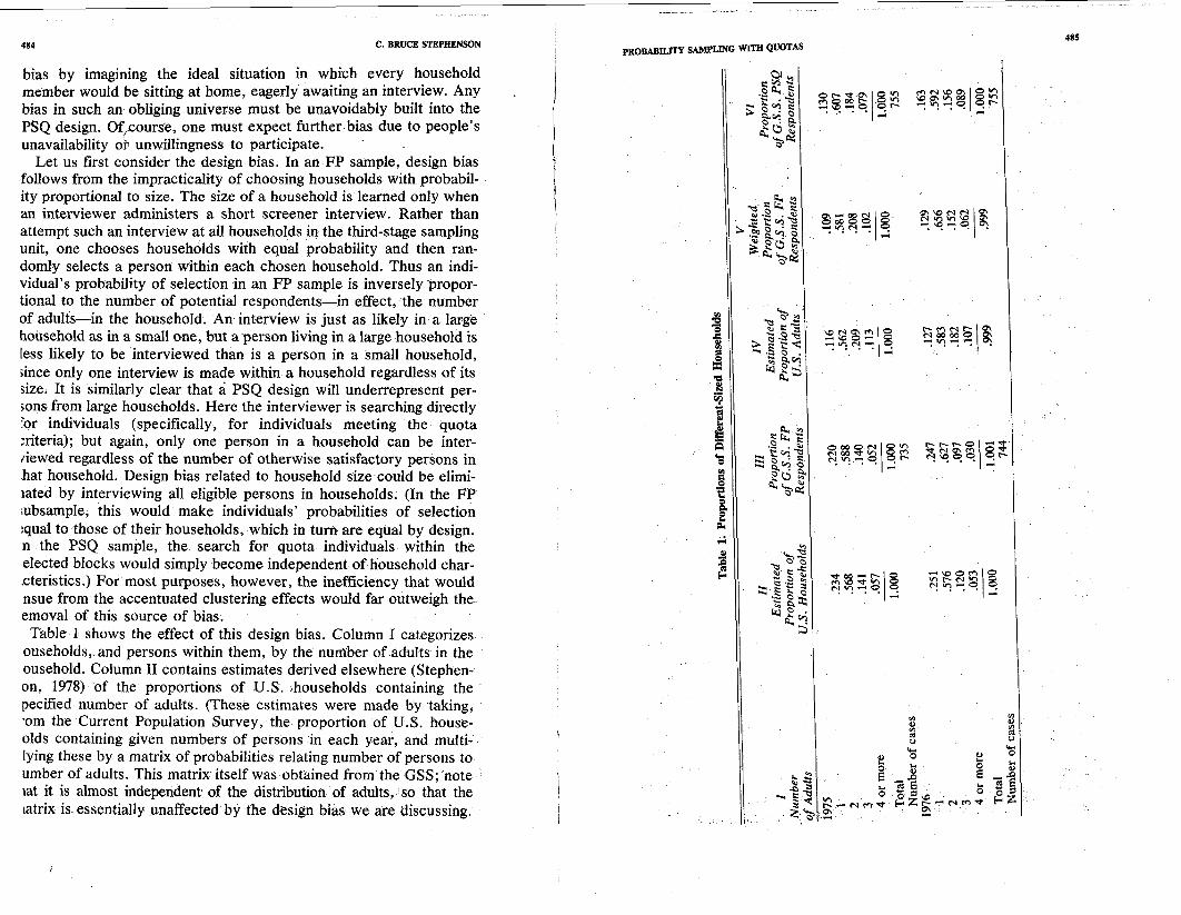
Table 1 shows the effect of this design bias. Column I categorizes ouseholds, and persons within them, by the number of adults in the ousehold. Column I1 contains estimates derived elsewhere (Stephen- on, 1978) of the proportions of U.S. bhouseholds containing the pecified number of adults. (These estimates were made by taking, -om the Current Population Survey, the proportion of U.S. house- olds containing given numbers of persons in each year, and multi- lying these by a matrix of probabilities relating number of persons to umber of adults. This matrix itself was obtained from the GSS; note lat it is almost independent of the distribution of adults, so that the tatrix is essentially unaffected by the design bias we are discussing.

PROBABILITY SAMPLMG WITH QUOTAS 485

486 C. BRUCE STEPAENSON

However, the stability of the numbers in Column I1 is dependent upon the case base for the corresponding row of the matrix. Hence the smaller numbers in Column II are the least stable.) Column 111, by comparison, shows the measured distribution of respondents' house- hold sizes in the FP subsamples of the GSS. By weighting the proportions in Columns I1 and 111 with their respective numbers of adults, we obtain in Columns IV and V estimates of the proportions of U.S. adults residing in households with the given number of adults. Here weights of 4.0 were used for all households with four or more adults. More accurate estimates would require using the exact number of adults, but these are not necessary for our present comparative purposes. The proportions, in Columns I11 and V, for the FP subsam- ples match our expectations reasonably well: unweighted, they are a good estimate of the distribution of households by size; weighted, they are a good estimate of the distribution of adults by household size.

Column VI shows the proportions obtained in the PSQ subsam- ples. The expected bias against persons from large households is evident in the comparison of Columns VI and IV. However, when individuals are the units of analysis and the data are used unweighted-as appears to be the case in most published research- the proportions from the PSQ subsample are less biased than those From the FP subsample. Column VI is closer to Column IV than is 2olumn 111. (See Stephenson, 1978, for discussion of why this is so.)

Bias in the proportion of respondents from different-sized house- holds is not very important in most analysis. The bias will, however, be transmitted with weakened intensity to other variables that are -elated to household size. Some of these are shown in Table 2. The 'elationship to number of adults of the first two variables in the table, otal number of persons and number of persons earning money, is )bvious. As Table 2 shows, the relative lack of persons from large louseholds in the FP subsample, as compared to the PSQ, persists in )oth of these variables. The remaining two items in Table 2, propor- ion married and proportion Catholic, are more important substan- ively but less strongly related to number of adults in the household. :ombining the two surveys, the proportions married in households of , 2, 3, and 4+ adults are respectively .02, .89, .62, and 53; the roportions Catholic are .23, .24, .27, and .37. For these variables 'able 2 shows that the expected differences are present but small ach year. Their "statistical significance," or lack thereof, is irrele- ant in this context, since they are transmitted from the known :lationship of household size to sampling technique. A precise correction for the design bias is available for the FP

PROBABILITY SAMPLING WITH QUOTAS 487

Table 2. Selected Variables by Subsample

1975 1976

FP PSO FP PSQ

Number of persons in households

1 .I70 .099 .I86 .128 2 .298 .293 .327 .317 3 .I96 .208 .I62 .I81 4 .I59 .I81 .I54 .I63 5 .lo2 .I11 .I11 .I18 6 or more .075 .lo7 -- .061 .093 --

Total 1.000 .999 1.001 1.000 Cases 735 755 742 755

Number of persons earning money in household 0 ,144 .I27 .I73 .I40 1 .417 .384 .436 .405 2 .310 .341 .300 .303 3 .073 .090 .063 .095 4 or more .056 .057 -- -- .028 .057

Total 1.000 .999 1.000 1.000 Cases 729 753 741 750

Marital status Married .650 .694 .641 .658 Not mamed .350 .306 -- .359 .342 --

Total 1.000 1.000 1.000 1.000 Cases 735 755 744 755

Religion Catholic .222 .265 .247 .274 Non-Catholic .778 .735 -- .753 .726 --

Total 1.000 1.000 1.000 1.000 Cases 734 754 742 755

subsample: one simply weights by number of adults, as we did in Column V of Table 1. The weighted sample proportions will still differ from the true proportions because of sampling error and (unknown), participation bias, but these are typically much smaller than the de-

I sign bias. Such weighting is, of course, inappropriate for the FP subsample whenever the household, rather than the individual re-

\ spondent, is the unit of analysis. There is no equally neat method for correcting the design bias in the PSQ subsample. This bias, against persons from large households, is expected; but a theoretical estima-

I tion of its size would be a formidable task. If accurate representation of different-sized households is required from a PSQ one must resort

I to "post-stratification" by simply weighting one's sample to match the population proportions, or estimates of them.

488 C. BRUCE STJ3PHENSON

Since each sample design, before weighting, is expected to yield biased proportions of persons from different-sized households, all the subsample comparisons examined in the present research were re- peated with weights which compensated, so far as possible, for the design bias related to household size. Application of these weights eliminated the subsample differences in total household size, number of money-earners per household, and proportion married; and it re- duced the size of the differences in proportion Catholic. These vari- ables aside, weighting had no systematic effect on differences be- tween the FP and PSQ subsamples. We shall therefore continue to discuss the unweighted comparisons.

Further bias, in either sample, originates from people being un- available or unwilling to participate. In most cases, elusive or reluc- tant respondents will be more seriously underrepresented in a PSQ sample than in an FP, because the field staff will put considerable effort into locating a person selected as an FP respondent and con- vincing that person to participate. Failures to find or convince such people are known, counted, and included in the nonresponse rate. On the other hand, interviewers in a PSQ survey simply go next door when no suitable person is available at a household. In general, then, people who are difficult to locate or to interview will be more seri- ously underrepresented in a PSQ than in an FP sample; yet the PSQ design permits no estimate of their number.

This general situation is modified somewhat for certain variables whose sample distribution is completely specified by the PSQ design. The quota categories, in particular, will be entirely filled, since the sample is not complete until they are filled. The "representation" thus attained is imperfect, however. Persistence in filling the quotas of, say, men younger than thirty-five is useful only to the extent that men younger than thirty-five are a homogeneous group. In the terms of Sudman's argument cited earlier, this criterion reduces to the familiar fact that stratification is useful only to the extent that strata are homogeneous. Now, the homogeneity of the "strata" formed by the quota categories depends upon one's substantive interests. Re- searchers who are studying some phenomenon strongly related to sex, but who are not primarily interested in its relationship to sex, will benefit from the quota controls that ensure proportionate representa- tion of men and women in a PSQ sample. If an FP sample contains too few men, because of a differential response rate perhaps, the same benefit can be achieved by post-stratification, that is, by re- weighting the sample to correct the sex distribution. Of course, a sample stratum that is present in its correct proportion because of either quota controls or post-stratification will not necessarily repre-

PROBABILITY SAMPLMG WITH QUOTAS 489

sent the corresponding population stratum well. No sample can be made to reflect the characteristics of population groups that are not included in it.

Turning to the data: the General Social Surveys included an inter- viewer rating of the cooperation shown by respondents who actually did participate. The four categories range from "friendly and in- terested" to "hostile." Interviewers have consistently rated over 80 percent of the sample "friendly and interested." In each of the 1975-76 surveys the proportion receiving less than this rating was about 4 percent higher in the FP subsample than in the PSQ. This might represent only the irritation of interviewers at the sometimes considerable effort needed to obtain completed FP interviews; but it certainly seems to confirm our expectation that FP techniques will obtain more interviews from less cooperative persons. Better repre- sentation of these persons is an advantage for the FP technique, one which would increase in research where respondent cooperation is a problem.

The four categories used in assigning quotas in the present PSQ design (men under thirty-five, men thirty-five and older, employed women, and unemployed women) were chosen because of the ex- pectation, based on previous research, that sex, age, and employment defined population groups difficult to interview (Sudman, 1966:752). In fact, the FP subsamples included about 58 percent women each year, compared to 52-53 percent in the quota-controlled PSQ. Evi- dently, more men than women were either unavailable or unwilling to be interviewed in the FP subsamples. Adjustment of the FP subsam- ple by weighting would eliminate this bias in research where it is important. Neither the unweighted PSQ nor the weighted FP subsam- ple, of course, will represent the truly uncooperative men.

A different pattern appears when one examines employment status. This is quota-controlled for women in the PSQ subsamples, but not for men. Table 3 shows that there are no subsample differences among women, while there are rather large differences among men. Assuming that the quotas for employed women are correct, it appears that the callback procedures in the FP subsample successfully achieve a representative proportion of employed women. It also appears that the lack of control over employment status for men in the PSQ sample has permitted a 10-15 percent deficiency in men who are working fulltime. PSQ interviewers were instructed to interview only at times when people are likely to be at home, late afternoons, evenings, and weekends; yet they evidently encountered an excess of the more readily available men, those not working fulltime.

No. similar problem accompanies the control which is applikd to

490 C. BRUCE STEPAENSON

men but not to women, age. There are no age differences between the subsamples for either sex. Optimistically, this means that no age quotas are needed for women, and the FP technique successfully obtains interviews from people of all ages.

One final, less obvious sense in which the composition of the PSQ subsample is controlled is that the choice of segments, when the sample is drawn, determines the geographic composition of the sam- ple. The quotas ensure that five cases, in the present design, are obtained from each segment. In an FP sample, on the other hand, the number of cases assigned in a segment, but not the number com- pleted, is determined before interviewing begins. If people in a par- ticular segment turn out to be less cooperative (or less easily located) than expected, there will simply be fewer cases than expected from that segment. More generally, if the response rate is low in certain kinds of segments, the achieved (FP) sample will underrepresent people from those kinds of segments. Thus central-city neighborhoods have yielded lower response rates, in several studies, than other places (see Marquis, 1977: 11-13 and Table 6; also Table 1 in Sudman, 1966). This fact will not visibly affect a PSQ sample, where interviewers can 3btain the desired number of cases from any neighborhood by con- :inuing to canvass. An FP sample, on the other hand, will be deficient n people from neighborhoods with low response rates.

Direct examination of this problem would require consideration of he actual refusals and other noninterviews, if possible in conjunction with the number of calls required to fill PSQ quotas in various neigh- )orhoods. We do not have data for such analysis. The following facts, lowever, suggest that the FP subsarnples actually were deficient in

Table 3. Employment Status by Subsample by Sex

Women Men

FP PSQ FP PSQ

975 Working fulltime Working parttime Other

Total Cases

!976 Working fulltime Working parttime Other

Total 1.000 1.000 1.001 1.000 Cases 430 400 314 355

PROBABXLlTY SAMPLMG WITE QUOTAS 491

cases from central cities. In each of the 1975 and 1976 FP subsamples, the average number of cases per segment was 5.0. Segments from central cities with populations greater than 250,000 (about a fifth of all segments used in the surveys) averaged 4.1 cases in 1975, 4.2 in 1976; segments from the central cities of the 12 largest Standard Metropoli- tan Statistical Areas (about an eighth of the segments) averaged 3.1 cases in 1975, 4.3 in 1976. Evidently the achieved cluster sizes are smaller in large central cities.

One must interpret this finding with some caution. The situation we have described differs from more typical nonresponse problems only insofar as one is dealing with attributes of the neighborhood itself. In an FP sample the effect of nonresponse is the same on neighborhood characteristics as on individual ones: any attribute concentrated among persons who are difficult to find or interview will be underrep- resented. PSQ sampling techniques, by requiring that a specific number of interviews be obtained in every sampled neighborhood, ensure that attributes of a neighborhood will be represented (via its inhabitants) regardless of whether neighborhood residents are difEcult to find or- interview. Thus a neighborhood fbll of unusually belligerent people will be represented properly in a PSQ sample, but not necessarily the belligerent people themselves; for the respondents finally interviewed may well be among the most amiable in the neighborhood. This example is exactly analogous to the earlier discussion of the artificial representation of variables used for the quota controls. On the other hand, if people in big cities favor federal aid to cities, then the forced representation of central-city neighborhoods in a PSQ sample would effectively capture proponents of federal aid to cities. In an FP sam- ple, a low central-city response rate could bias the results against such aid, if the sample was not weighted to compensate. Here the effectiveness of the PSQ "neighborhood quotas" is obviously due to homogeneity of neighborhoods with respect to the characteristic being examined.

We may tentatively suggest three GSS variables (in addition to the size-of-place codes themselves) where small subsample differences may be related to the problem of low central-city response rates. First, a smaller proportion of the FP subsamples favored spending on problems of the cities, and as suggested above it is particularly big-city residents who support such spending. Second, people who can name their ethnicity tend to live in large cities, and each year a smaller proportion of the FP subsamples named an ethnicity. Finally, all religious groups except Protestants are to some extent concen- trated in large cities; such groups are perhaps slightly underrepre- sented in FP samples.

12 C. BRUCE STEPHENSON

Statistical Summary

As promised, we shall now compare our best estimate of the umber of statistically significant subsample differences with the umber expected under a very broad null hypothesis: that, with stated xceptions, the two sampling techniques measure the same (uni- ariate) distributions for all variables on the surveys. Of course, this ypothesis cannot be strictly true: we know of some real differences, nd these must be transmitted to other variables. Still, the general mroposition suffices for our purposes. First, the exceptions. In the cross-tabular analysis, significant dif-

Srences were found between the subsamples for employment status, ex, and number of adults in the household. As explained above, we elieve these differences to be real. Two further variables, number of ersons and number of persons earning money in the household, robably show real dBerences, although the corrected chi-squares {ere not statistically significant at the .05 level. Finally, the dif- Srences in the three size-of-place codes are quite possibly real, and in ny case are not appropriate for these aggregate comparisons. Sub- -acting these 16 comparisons (eight variables, two years) from the 73 crosstabular comparisons done originally, we retained 457 com- arisons on which to check the general null hypothesis. Twenty-four f these (.053 of the total) were statistically significant at the .05 level, nd six (.013 of the total) at the .O1 level. Moreover, several of the ignificant differences involved the highly artificial dichotomies which {ere created to preserve subsample differences while permitting the alculation of design effects. In the aggregate, then, these remaining ariables were distributed randomly between the subsamples. Turning to the tests for differences in subsample means, we found a

lore complex situation. After removing from consideration the num- ers of adults, persons, and money-earners in the household, and the ize-of-place codes, we were left with 141 tests for differences be- ween means. Twenty-two of these (. 156 of the total) were statistically ignificant at the .05 level. It was quite clear from the start that many of the "statistically

ignificant" differences between the subsample means could not be =a1 differences due to sampling technique: they changed direction etween 1975 and 1976. In fact, many of the GSS variables measured t or near the interval level are measures of social, economic, or ducational status. On nearly all of these measures the FP subsample anked higher in 1975, but the PSQ subsample ranked higher in 1976. bidently a shift in the subsample distribution of these highly corre- ited variables took place between the two years. The reversa1 is Irtunate, for without it we might have been left with all sorts of fears

PROBABlLlTY SAMPLING WITH QUOTAS 493

about education or income biases in one or the other type of sample. The size of the reversal is slightly embarrassing, since we have mea- sured it so many times. If there are no large status differences be- tween the "universes" sampled by the two techniques, why did so many turn up in our two surveys? This question necessitates a brief digression in defense of probability (theory, which may profitably be skipped by any readers who are not bothered by the question.

As implied above, the reason so many variables which do not really differ between subsamples showed statistically significant differences is just that the variables, far from being independent, all measured about the same thing. The significance tests were trying to lead us into a "Type I" error, as they are expected to do a known proportion of the time. We insisted on testing all the status measures, and, as it happened, fell into the same Type I error repeatedly.

The variables which seem particularly likely to be involved in this sort of thing are education of respondent, spouse, father, and mother; Hodge-Siegel-Rossi occupational prestige of respondent's and spouse's jobs; family and respondent income; educational require- ments and relationship to data of respondent's and spouse's jobs; and Temme prestige of respondent's and spouse's jobs. (See Davis, Smith, and Stephenson, 1978, for precise definitions of these mea- sures.) These are all, of course, different variables. They are highly correlated, however, and highly clustered in neighborhoods. We have proposed that the (conceptual) variable status, as measured by the 14 variables listed above, was responsible for most of the observed subsample differences in these variables. We therefore performed a complete principal-components analysis of the 14 measured variables each year. The complete principal-components solution has the char- acteristic that the 14 factors are merely a linear transformation of the original 14 variables; no information has been lost or gained. The factor solutions for the two years were almost identical: each year the first factor accounted for 47-49 percent of the variance, with most loadings above .7; each year this principal factor was highly clustered, with a design effect greater than two. We therefore replaced, each year, the 14 correlated original variables with the 14 equivalent but statistically independent factors. (Had this paper attempted to main- tain a strictly inferential methodology throughout, we would have needed some simirar control over the lack of independence among hundreds of variables: a formidable task.) Only 2 of the 28 compari- sons, adjusted for clustering, made on the independent factors were statistically significant at the .05 level. The principal factor was "sig- nificantly" higher in the FP subsample in 1975; the second factor, which involves residual variation in respondent's occupation as con-

494 C. BRUCE STEPHENSON I

trasted with spouse's occupation, was "significantly" higher in the PSQ subsample in 1976. Neither difference was consistent across the two years. We do not present details of the factor analysis, as it is uninteresting in itself and readily reproducible from the public data.

If we count 2, instead of 15, significant differences at the .05 level on these 14 variables for the two years, the aggregate results looked much more reasonable. Nine comparisons out of 141 (.064) remained statistically significant at the .05 level, and two (.014) at the .O1 level.

The GSS variables not discussed in the text thus present, in the aggregate, a statistical picture compatible with our general null hy- pothesis. They do not appear to be distributed dBerently in the PSQ subsamples and in the FP subsamples. This is an oversimplification, since the real differences in household size, sex, employment status, and perhaps central-city representation are certainly transmitted to other variables. Such indirect differences are evidently small.

Conclusion

Three of our substantive findings are worth repeating. First, the selection procedures choose markedly different samples with regard to household size. The PSQ sample overrepresents large households, while both samples, especially the (unweighted) FP, underrepresent people from large households. Second, the PSQ sample in its present form underrepresents men who are working fulltime. Finally, difficult respondents are probably underrepresented more seriously in the PSQ sample, except in true neighborhood characteristics, where the PSQ design-but not the FP--ensures that the sampled neighborhoods are represented in the desired proportions. A weighted FP sample should represent neighborhoods as well as a PSQ sample, even in these instances. Sudman (1966), with less data for empirical comparison, identified the household-size bias and the sex difference due to un- cooperative men.

We have looked only for univariate effects, except for the employ- ment difference which occurred only among men; and of course we have examined only variables which appeared on the 1975 or 1976 General Social Surveys. We do not expect multivariate effects will be large. However, it is certainly possible that other variables exist whose distribution is affected by the type of sample used to measure them.

It should be emphasized that our findings apply only to "probability sampling with quotas" as described by Sudman. Other "quota sam- ples" that lack the tight geographic controls of the PSQ design cannot be assumed to behave as'well as the latter.

PROBABILZN SAMPLMG WITH QUOTAS 495

Nonetheless, the principal conclusion from this research is surely that the data from a survey carefully conducted with a PSQ design are, in fact, well-behaved. Survey analysis has been performed, and will no doubt continue to be performed, on PSQ samples, with conse- quences far less pernicious than one would expect from a reading of the more impassioned indictments of "quota sampling" (most of which, indeed, were directed at the far more discretionary quota samples of the 1940s and 1950s). It appears to us that a PSQ sample can represent its universe quite well, although it carries a greater risk of bias from the exclusion of people who are hard to fmd or interview. This risk should be frankly acknowledged, and in some cases will certainly outweigh the extra cost of an FP sample. Yet with a few exceptions, there was no detectable bias in the large group of ques- tions included on the GSS. It is likely that a quota control on the most serious exception, employment status for men, would 'appreciably improve the quality of PSQ samples. Still, one has better sources than these surveys for estimates of labor force participation, and indirect effects of this deficiency, although undoubtedly present, were not found to be large.

As to the theoretical question whether statistical inference is properly applied to samples chosen with an element of interviewer discretion, we have said nothing. We heartily endorse the idea that researchers should think about this and related questions. We do not believe, however, that among the many ways people misuse inferen- tial statistics, their application to PSQ samples is a matter for great concern.

References

Cohen, Joel E. 1976 "The distribution of the chi-squared statistic under clustered sam-

pling from contingency tables." Journal of the American Statistical Association 71 :665-70.

Davis, James A. 1975 Codebook for the Spring 1975 General Social Survey. Chicago: Na-

tional Opinion Research Center. 1976 Codebook for the Spring 1976 General Social Survey. Chicago: Na-

tional Opinion Research Center. Davis, James A., Tom W. Smith, and C. Bruce Stephenson

1978 General Social Surveys, 1972-1978: Cumulative Codebook. Chicago: National Opinion Research Center.

King, Benjamin F., and Carol Richards 1972 "The 1972 NORC national probability sample." Chicago: National

Opinion Research Center (photocopy). Kish, Leslie.

1965 Survey Sampling. New York: Wiley.

496 C. BRUCE STEPHENSON

Marquis, Kent H. 1977 "Survey response rates: some trends, causes and correlates." Santa

Monica: The Rand Corporation, The Rand Paper Series, P-5863. Moser, C. A.

1952 "Quota sampling." Journal of the Royal Statistical Society, Series A, 115:411-23.

Moser, C. A., and A. Stuart 1 1953 "An experimental study of quota sampling." Journal of the Royal

Statistical Society, Series A, 116:349-405. Shuster, J. J., and D. J. Downing

1976 "Two-way contingency tables for complex sampling schemes." Biometrika, 63:271-76.

Smith, Tom W. 1975 "Response rates on the 1975-1978 General Social Surveys with

comparisons to the omnibus surveys of the Survey Research Center, 1972-1976." Chicago: National Opinion Research Center, GSS Technical Report #7.

Stephan, Frederick J., and Philip J. McCarthy 1958 Sampling Opinions. New York: Wiley.

Stephenson, C. Bruce 1978 "Weighting the General Social Surveys for bias related to house'hold

size." Chicago: National Opinion Research Center, GSS Technical Report #3.

Sudman, Seymour 1966 "Probability sampling with quotas." Journal of the American Statis-

tical Association. 61 :749-71.