In the format provided by the authors and unedited.

© 2017 Macmillan Publishers Limited, part of Springer Nature. All rights reserved.

SUPPLEMENTARY INFORMATIONDOI: 10.1038/NCLIMATE3277

NATURE CLIMATE CHANGE | www.nature.com/natureclimatechange

LETTERSPUBLISHED ONLINE: 24 APRIL 2017 | DOI: 10.1038/NCLIMATE3277

Weakening temperature control on theinterannual variations of spring carbon uptakeacross northern landsShilong Piao1,2,3*, Zhuo Liu2, TaoWang1,3, Shushi Peng2, Philippe Ciais4, Mengtian Huang2,Anders Ahlstrom5, John F. Burkhart6, Frédéric Chevallier4, Ivan A. Janssens7, Su-Jong Jeong8,Xin Lin4, Jiafu Mao9, John Miller10,11, Anwar Mohammat12, Ranga B. Myneni13, Josep Peñuelas14,15,Xiaoying Shi9, Andreas Stohl16, Yitong Yao2, Zaichun Zhu2 and Pieter P. Tans10

Ongoing spring warming allows the growing season to beginearlier, enhancing carbon uptake in northern ecosystems1–3.Here we use 34 years of atmospheric CO2 concentrationmeasurements at Barrow, Alaska (BRW, 71◦ N) to show thatthe interannual relationship between spring temperature andcarbon uptake has recently shifted. We use two indicators: thespring zero-crossing date of atmospheric CO2 (SZC) and themagnitudeofCO2 drawdownbetweenMayand June (SCC). Thepreviously reported strong correlation between SZC, SCC andspring land temperature (ST) was found in the first 17 yearsof measurements, but disappeared in the last 17 years. Asa result, the sensitivity of both SZC and SCC to warmingdecreased. Simulations with an atmospheric transport model4coupled to a terrestrial ecosystem model5 suggest that theweakened interannual correlation of SZC and SCC with ST inthe last 17 years is attributable to the declining temperatureresponse of spring net primary productivity (NPP) ratherthan to changes in heterotrophic respiration or in atmospherictransport patterns. Reduced chilling during dormancy andemerging light limitation are possible mechanisms that mayhave contributed to the loss of NPP response to ST. Our resultsthus challenge the ‘warmer spring–bigger sink’ mechanism.

For the past decade, boreal forests have been a net carbon sink6;but the sink-or-source status of arctic tundra cannot be deducedfrom current observations7. Both modelling and observationalstudies have shown that spring warming has advanced leaf onsetin the Northern Hemisphere, thus lengthening the photosynthesisseason and, in turn, strengthening net carbon uptake1–3,8. The effectof temperature on spring CO2 uptake by plants has been identifiedas the main mechanism explaining the year-to-year variationsof atmospheric CO2 in spring. For instance, at Point Barrow

(hereafter referred to as Barrow) atmospheric measurement stationin north Alaska, the periodical spring drawdown of atmosphericCO2 occurs earlier in the year when spring temperature is warmer1,9.Beyond the rather well-studied interannual variations, examplesof decadal changes in climate affecting ecosystems remain elusive.Limited evidence from tree-ring data10 and satellite vegetationgreenness11,12 does give hints that the response of northern terrestrialcarbon fluxes to temperature may not be constant over timescalesof decades.

Here, we investigate changes in the interannual relationshipbetween spring temperature and CO2 uptake by northernecosystems (NEP, net ecosystem productivity) over the past threedecades. We use: the longest high-latitude atmospheric CO2record from Barrow; the LMDZ4 (Laboratoire de MétéorologieDynamique, ‘Z’ stands for zoom) atmospheric transport model4simulating CO2 concentrations from NEP produced by theprocess-based terrestrial carbon model ORCHIDEE5 (ORganizingCarbon and Hydrology In Dynamic Ecosystems), which alsoallows the partitioning of NEP into its component fluxes of NPPand heterotrophic respiration (HR); and satellite observationsof vegetation greenness, a proxy for photosynthesis. Temporalvariations in the seasonal variability of CO2 in spring at Barrowreflect changes in northern NEP and atmospheric mixing1,13. Weconsider two indicators of spring CO2 variations at Barrow, namelythe SZC (the day of year when CO2 crosses down through itsannual mean level; Supplementary Figs 1 and 2a) and the SCC(spring carbon capture, the seasonal magnitude of the observedCO2 decrease between the first week of May and the last week ofJune; Supplementary Figs 1 and 2b)1,13,14. These two indicators arecorrelated with land temperature to give the response of springNEP to temperature (all variables are detrended, see Methods).

1Key Laboratory of Alpine Ecology and Biodiversity, Institute of Tibetan Plateau Research, Chinese Academy of Sciences, Beijing 100085, China.2Sino-French Institute for Earth System Science, College of Urban and Environmental Sciences, Peking University, Beijing 100871, China. 3Center forExcellence in Tibetan Earth Science, Chinese Academy of Sciences, Beijing 100085, China. 4Laboratoire des Sciences du Climat et de l’Environnement, CEACNRS UVSQ, Gif-sur-Yvette 91191, France. 5School of Earth, Energy and Environmental Sciences, Stanford University, Stanford, California 94305-2210,USA. 6Department of Geosciences, University of Oslo, PO Box 1047 Blindem, 0316 Oslo, Norway. 7Department of Biology, University of Antwerp,Universiteitsplein 1, 2610Wilrijk, Belgium. 8School of Environmental Science and Engineering, South University of Science and Technology of China,Shenzhen 518055, China. 9Climate Change Science Institute and Environmental Sciences Division, Oak Ridge National Laboratory, Oak Ridge,Tennessee 37831, USA. 10National Oceanic and Atmospheric Administration Earth Systems Research Laboratory (NOAA/ESRL), 325 Broadway, Boulder,Colorado 80305, USA. 11Cooperative Institute for Research in Environmental Sciences, University of Colorado, Boulder 80309, USA. 12Xinjiang Institute ofEcology and Geography, Chinese Academy of Sciences, Urumqi 830011, Xinjiang, China. 13Department of Earth and Environment, Boston University, 675Commonwealth Avenue, Boston, Massachusetts 02215, USA. 14CREAF, Cerdanyola del Valles, Barcelona 08193, Catalonia, Spain. 15CSIC, Global EcologyUnit CREAF-CEAB-CSIC-UAB, Cerdanyola del Valles, Barcelona 08193, Catalonia, Spain. 16NILU—Norwegian Institute for Air Research,PO Box 100, 2027 Kjeller, Norway. *e-mail: slpiao@pku.edu.cn

NATURE CLIMATE CHANGE | ADVANCE ONLINE PUBLICATION | www.nature.com/natureclimatechange 1

© 2017 Macmillan Publishers Limited, part of Springer Nature. All rights reserved.

LETTERSPUBLISHED ONLINE: 24 APRIL 2017 | DOI: 10.1038/NCLIMATE3277

Weakening temperature control on theinterannual variations of spring carbon uptakeacross northern landsShilong Piao1,2,3*, Zhuo Liu2, TaoWang1,3, Shushi Peng2, Philippe Ciais4, Mengtian Huang2,Anders Ahlstrom5, John F. Burkhart6, Frédéric Chevallier4, Ivan A. Janssens7, Su-Jong Jeong8,Xin Lin4, Jiafu Mao9, John Miller10,11, Anwar Mohammat12, Ranga B. Myneni13, Josep Peñuelas14,15,Xiaoying Shi9, Andreas Stohl16, Yitong Yao2, Zaichun Zhu2 and Pieter P. Tans10

Ongoing spring warming allows the growing season to beginearlier, enhancing carbon uptake in northern ecosystems1–3.Here we use 34 years of atmospheric CO2 concentrationmeasurements at Barrow, Alaska (BRW, 71◦ N) to show thatthe interannual relationship between spring temperature andcarbon uptake has recently shifted. We use two indicators: thespring zero-crossing date of atmospheric CO2 (SZC) and themagnitudeofCO2 drawdownbetweenMayand June (SCC). Thepreviously reported strong correlation between SZC, SCC andspring land temperature (ST) was found in the first 17 yearsof measurements, but disappeared in the last 17 years. Asa result, the sensitivity of both SZC and SCC to warmingdecreased. Simulations with an atmospheric transport model4coupled to a terrestrial ecosystem model5 suggest that theweakened interannual correlation of SZC and SCC with ST inthe last 17 years is attributable to the declining temperatureresponse of spring net primary productivity (NPP) ratherthan to changes in heterotrophic respiration or in atmospherictransport patterns. Reduced chilling during dormancy andemerging light limitation are possible mechanisms that mayhave contributed to the loss of NPP response to ST. Our resultsthus challenge the ‘warmer spring–bigger sink’ mechanism.

For the past decade, boreal forests have been a net carbon sink6;but the sink-or-source status of arctic tundra cannot be deducedfrom current observations7. Both modelling and observationalstudies have shown that spring warming has advanced leaf onsetin the Northern Hemisphere, thus lengthening the photosynthesisseason and, in turn, strengthening net carbon uptake1–3,8. The effectof temperature on spring CO2 uptake by plants has been identifiedas the main mechanism explaining the year-to-year variationsof atmospheric CO2 in spring. For instance, at Point Barrow

(hereafter referred to as Barrow) atmospheric measurement stationin north Alaska, the periodical spring drawdown of atmosphericCO2 occurs earlier in the year when spring temperature is warmer1,9.Beyond the rather well-studied interannual variations, examplesof decadal changes in climate affecting ecosystems remain elusive.Limited evidence from tree-ring data10 and satellite vegetationgreenness11,12 does give hints that the response of northern terrestrialcarbon fluxes to temperature may not be constant over timescalesof decades.

Here, we investigate changes in the interannual relationshipbetween spring temperature and CO2 uptake by northernecosystems (NEP, net ecosystem productivity) over the past threedecades. We use: the longest high-latitude atmospheric CO2record from Barrow; the LMDZ4 (Laboratoire de MétéorologieDynamique, ‘Z’ stands for zoom) atmospheric transport model4simulating CO2 concentrations from NEP produced by theprocess-based terrestrial carbon model ORCHIDEE5 (ORganizingCarbon and Hydrology In Dynamic Ecosystems), which alsoallows the partitioning of NEP into its component fluxes of NPPand heterotrophic respiration (HR); and satellite observationsof vegetation greenness, a proxy for photosynthesis. Temporalvariations in the seasonal variability of CO2 in spring at Barrowreflect changes in northern NEP and atmospheric mixing1,13. Weconsider two indicators of spring CO2 variations at Barrow, namelythe SZC (the day of year when CO2 crosses down through itsannual mean level; Supplementary Figs 1 and 2a) and the SCC(spring carbon capture, the seasonal magnitude of the observedCO2 decrease between the first week of May and the last week ofJune; Supplementary Figs 1 and 2b)1,13,14. These two indicators arecorrelated with land temperature to give the response of springNEP to temperature (all variables are detrended, see Methods).

1Key Laboratory of Alpine Ecology and Biodiversity, Institute of Tibetan Plateau Research, Chinese Academy of Sciences, Beijing 100085, China.2Sino-French Institute for Earth System Science, College of Urban and Environmental Sciences, Peking University, Beijing 100871, China. 3Center forExcellence in Tibetan Earth Science, Chinese Academy of Sciences, Beijing 100085, China. 4Laboratoire des Sciences du Climat et de l’Environnement, CEACNRS UVSQ, Gif-sur-Yvette 91191, France. 5School of Earth, Energy and Environmental Sciences, Stanford University, Stanford, California 94305-2210,USA. 6Department of Geosciences, University of Oslo, PO Box 1047 Blindem, 0316 Oslo, Norway. 7Department of Biology, University of Antwerp,Universiteitsplein 1, 2610Wilrijk, Belgium. 8School of Environmental Science and Engineering, South University of Science and Technology of China,Shenzhen 518055, China. 9Climate Change Science Institute and Environmental Sciences Division, Oak Ridge National Laboratory, Oak Ridge,Tennessee 37831, USA. 10National Oceanic and Atmospheric Administration Earth Systems Research Laboratory (NOAA/ESRL), 325 Broadway, Boulder,Colorado 80305, USA. 11Cooperative Institute for Research in Environmental Sciences, University of Colorado, Boulder 80309, USA. 12Xinjiang Institute ofEcology and Geography, Chinese Academy of Sciences, Urumqi 830011, Xinjiang, China. 13Department of Earth and Environment, Boston University, 675Commonwealth Avenue, Boston, Massachusetts 02215, USA. 14CREAF, Cerdanyola del Valles, Barcelona 08193, Catalonia, Spain. 15CSIC, Global EcologyUnit CREAF-CEAB-CSIC-UAB, Cerdanyola del Valles, Barcelona 08193, Catalonia, Spain. 16NILU—Norwegian Institute for Air Research,PO Box 100, 2027 Kjeller, Norway. *e-mail: slpiao@pku.edu.cn

NATURE CLIMATE CHANGE | ADVANCE ONLINE PUBLICATION | www.nature.com/natureclimatechange 1

© 2017 Macmillan Publishers Limited, part of Springer Nature. All rights reserved.

Figure S1 A schematic to describe the terms for characterizing spring carbon uptake. We

use a smoothed detrended annual cycle of CO2 (the black solid line) for the year 1979 at

Barrow. The horizontal dashed line represents the detrended mean CO2 concentration. The

two vertical dashed lines indicate the start and end of the spring carbon uptake period

(May-June). Spring zero crossing date (SZC) is defined as the day of the year when CO2

crosses down its annual mean level (marked in blue). Spring carbon capture (SCC) is

calculated as the seasonal magnitude of the observed CO2 decrease between the first week of

May and the last week of June (marked in red).

Figure S2 Temporal evolution of observed spring zero crossing date (SZC), spring

carbon capture (SCC) and the average spring (March-June) temperature over the

vegetated region north of 50oN (ST). a, SZC, b, SCC and, c, ST, from 1979 to 2012.

Figure S3 The partial correlation coefficient of a, SZC (RSZC) and b, SCC (RSCC) with

preseason temperature using different preseason periods. The preseason is defined as the

period before 30 June with different start months varying from November to June. All

variables are detrended before the partial correlation analysis. ** indicates statistically

significant at the 5% level and * statistically significant at the 10% level.

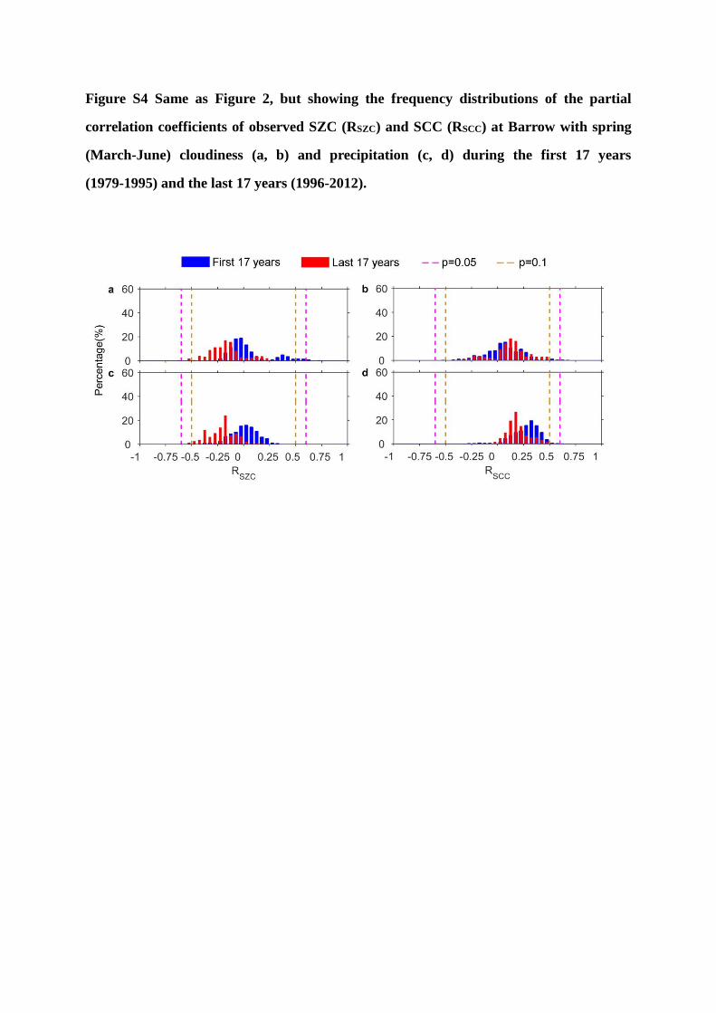
Figure S4 Same as Figure 2, but showing the frequency distributions of the partial

correlation coefficients of observed SZC (RSZC) and SCC (RSCC) at Barrow with spring

(March-June) cloudiness (a, b) and precipitation (c, d) during the first 17 years

(1979-1995) and the last 17 years (1996-2012).

Figure S5 Frequency distributions of the temperature sensitivity of (a) SZC (γSZC) and (b)

SCC (γSCC) at Barrow during the first 17 years (1979-1995; blue) and during the second,

more recent 17 years (1996-2012; red). The temperature sensitivity of SZC (SCC) is

calculated as the slope of temperature in a multiple regression of SZC (SCC) against

temperature, cloud cover and precipitation during March-June over the vegetated lands north

of 50 oN. The frequency distributions of temperature sensitivity are calculated by randomly

selecting 14 years during 1979-1995 and 1996-2012. All variables are detrended for each

study period before multiple linear regression analysis. Abbreviations of transport simulations

are defined in Table 1.

Figure S6 Mean spring footprint for Barrow derived from two different approaches

during three time periods. In the left panel, the footprint was derived from the adjoint code

of the LMDZ model. In the right panel, the footprint was derived from the Lagrangian particle

dispersion model FLEXPART. Note that the FLEXPART simulations are only available from

1985 to 2009.

Figure S7 Frequency distributions of the partial correlation coefficient of observed SZC

(RSZC) and SCC (RSCC) at Barrow with spring (March-June) temperature during the

first period (1979-1995) and during the second, more recent period (1996-2012). Here

climate variables (temperature, precipitation and cloud cover) were computed as the spatial

average weighted by the sensitivities (flux sensitivity from LMDZ and potential emission

sensitivity from FLEXPART) over the vegetated land area within the mean spring footprint. In

a-d, we used the mean spring footprint during the whole study period (1979-2012 for LMDZ

and 1985-2009 for FLEXPART, see Fig. S6 c and f). In e-h, we used the mean spring

footprint during the two time periods for the first 17 years and the last 17 years (Fig. S6 a, b,

d and e).

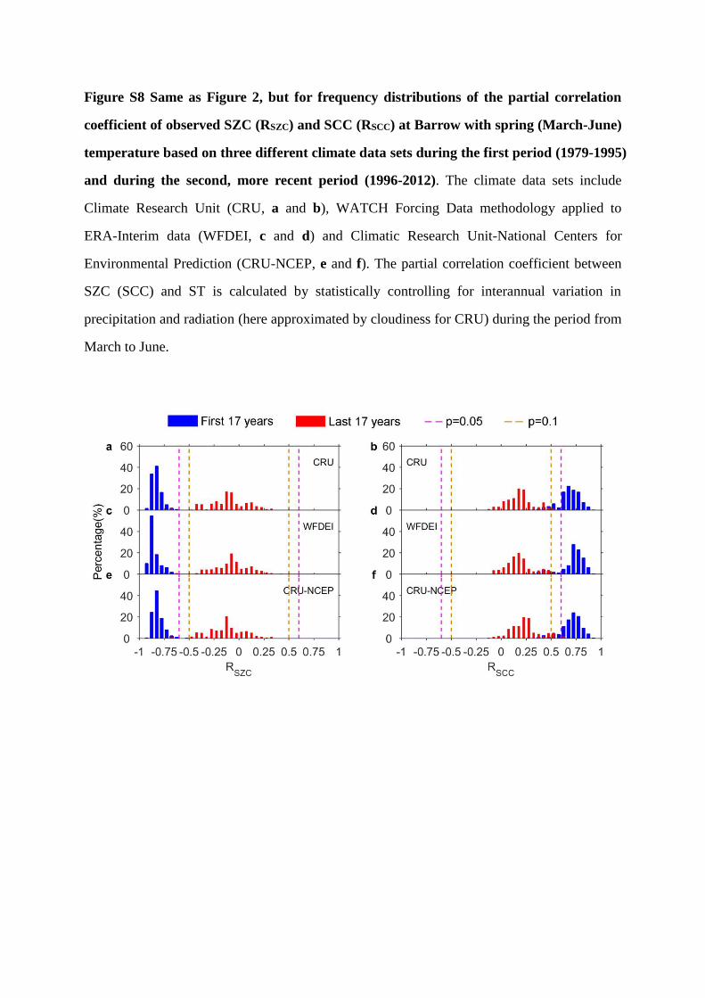
Figure S8 Same as Figure 2, but for frequency distributions of the partial correlation

coefficient of observed SZC (RSZC) and SCC (RSCC) at Barrow with spring (March-June)

temperature based on three different climate data sets during the first period (1979-1995)

and during the second, more recent period (1996-2012). The climate data sets include

Climate Research Unit (CRU, a and b), WATCH Forcing Data methodology applied to

ERA-Interim data (WFDEI, c and d) and Climatic Research Unit-National Centers for

Environmental Prediction (CRU-NCEP, e and f). The partial correlation coefficient between

SZC (SCC) and ST is calculated by statistically controlling for interannual variation in

precipitation and radiation (here approximated by cloudiness for CRU) during the period from

March to June.

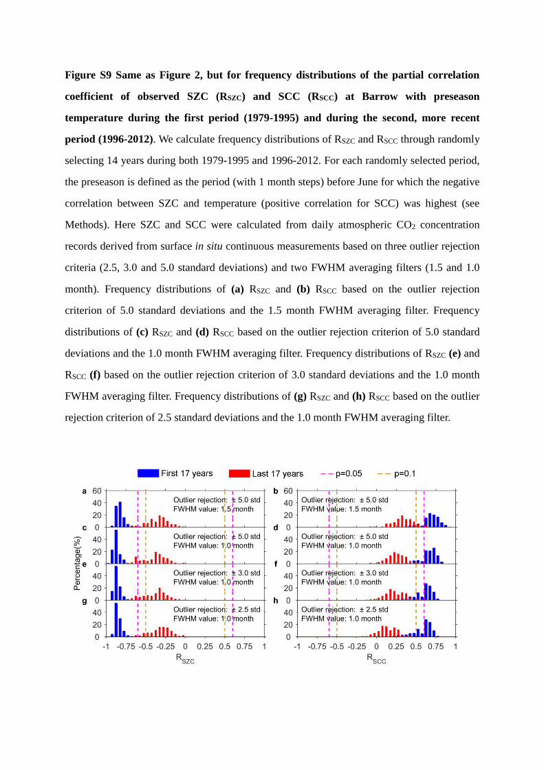
Figure S9 Same as Figure 2, but for frequency distributions of the partial correlation

coefficient of observed SZC (RSZC) and SCC (RSCC) at Barrow with preseason

temperature during the first period (1979-1995) and during the second, more recent

period (1996-2012). We calculate frequency distributions of RSZC and RSCC through randomly

selecting 14 years during both 1979-1995 and 1996-2012. For each randomly selected period,

the preseason is defined as the period (with 1 month steps) before June for which the negative

correlation between SZC and temperature (positive correlation for SCC) was highest (see

Methods). Here SZC and SCC were calculated from daily atmospheric CO2 concentration

records derived from surface in situ continuous measurements based on three outlier rejection

criteria (2.5, 3.0 and 5.0 standard deviations) and two FWHM averaging filters (1.5 and 1.0

month). Frequency distributions of (a) RSZC and (b) RSCC based on the outlier rejection

criterion of 5.0 standard deviations and the 1.5 month FWHM averaging filter. Frequency

distributions of (c) RSZC and (d) RSCC based on the outlier rejection criterion of 5.0 standard

deviations and the 1.0 month FWHM averaging filter. Frequency distributions of RSZC (e) and

RSCC (f) based on the outlier rejection criterion of 3.0 standard deviations and the 1.0 month

FWHM averaging filter. Frequency distributions of (g) RSZC and (h) RSCC based on the outlier

rejection criterion of 2.5 standard deviations and the 1.0 month FWHM averaging filter.

Figure S10 Same as Figure 2, but for frequency distributions of partial correlation

coefficient of observed SZC (RSZC) and SCC (RSCC) at Barrow with preseason

temperature based on weekly atmospheric CO2 concentration records during the first

period (1979-1995) and during the second, more recent period (1996-2012). Here the

weekly atmospheric CO2 concentration records were derived from (a, b) surface in situ

continuous measurements of SZC and SCC respectively, using the 1.5 month FWHM

averaging filter; and (c, d) surface flask samples of SZC and SCC respectively, using the 1.5

month FWHM averaging filter. We calculate frequency distributions of RSZC and RSCC

through randomly selecting 14 years during both 1979-1995 and 1996-2012. For each

randomly selected period, the preseason is defined as the period (with 1 month steps) before

June for which the negative correlation between SZC and temperature (positive correlation for

SCC) was highest (see Methods).

Figure S11 Frequency distributions of P value for the partial correlation coefficients of

observed SZC (PSZC) and SCC (PSCC) at Barrow with spring (March-June) temperature

considering the co-variation in snow water equivalent and previous winter temperature

during the first period (1979-1995) and during the second, more recent period

(1996-2012). Frequency distributions of P value of the partial correlation coefficient of (a)

SZC (PSZC) and (b) SCC (PSCC) with spring temperature after statistically controlling for

spring precipitation, spring cloud cover and maximum snow water equivalent from November

to June. Frequency distributions of P value of the partial correlation coefficient of (c) SZC

(PSZC) and (d) SCC (PSCC) with spring temperature after statistically controlling for spring

precipitation, spring cloud cover and winter (November to February) temperature. We

calculate frequency distributions of PSZC and PSCC through randomly selecting 14 years during

both 1979-1995 and 1996-2012. Note that snow water equivalent data is only available from

September 1979. Thus the maximum snow water equivalent from November 1978 to June

1979 was replaced by one value (null) when calculating P value of partial correlation

coefficient. Statistically significant P values are marked by the dotted line (magenta: P < 0.05

and brown: P < 0.1). The positive and negative sign indicate the corresponding positive and

negative partial correlation coefficients, respectively.

Figure S12 Frequency distributions of P value for the partial correlation coefficients of

observed SZC (PSZC) and SCC (PSCC) at Cold Bay (CBA) and Ocean Station M (STM)

with preseason temperature over the vegetated lands north of 50°N during the first

period (1979-1995) and during the second, more recent period (1996-2012). We calculated

frequency distributions of PSZC and PSCC using the 1.5 month FWHM averaging filter for (a, b)

CBA and (c, d) STM, respectively. The CO2 data at CBA and STM stations are based on

surface flasks sampled on a weekly basis. We calculate frequency distributions of PSZC and

PSCC through randomly selecting 14 years during 1979-1995 and 1996-2012. For each

randomly selected period, the preseason is defined as the period (with 1 month steps) before

June for which the negative correlation between SZC and temperature (positive correlation for

SCC) was highest (see Methods). Note that for STM, weekly CO2 records are only available

from 1981 to 2009. Thus all missing values were replaced by one value (null) when

calculating P value of partial correlation coefficient.

Figure S13 Changes in the partial correlation coefficients of a) SZC (RSZC) and (b) SCC

(RSCC) at Barrow with preseason (March-June) temperature over the vegetated lands

north of 50 oN during 1979-2012 after applying 15-year moving windows. The partial

correlation coefficient RSZC (RSCC) is computed as the correlation between the residuals

calculated after regressing SZC (SCC) on precipitation and cloud cover and those after

regressing ST on precipitation and cloud cover. Year on the horizontal axis is the central year

of the 15-year moving window (e.g., 1986 indicates a moving window from 1979-1993).

Solid circles indicate statistically significant partial correlation (P < 0.05), solid squares

indicate statistically marginally significant partial correlation (P < 0.1), and hollow circles

indicate insignificant partial correlation (P > 0.1). All variables are detrended for each study

period before partial correlation analysis. Abbreviations of transport simulations are defined

in Table 1.

Figure S14 Anomalies of observed and transport model simulated (a) SZC and (b) SCC

at Barrow from 1979 to 2012. Abbreviations of transport simulations are as defined in Table

1. TFTT: simulation with transient global NEE and transient transport; CFTT: simulation with

global NEE of year 1979 but transient transport (indicating the effect of wind change on SZC

and SCC variability); TFCT: the difference between TFTT and CFTT (indicating the effect of

global land carbon flux change on SZC and SCC variability); TFCT-B: the difference between

TFTT-B and CFTT (indicating the effect of boreal land carbon flux change on SZC and SCC

variability); TFCT-TE: the difference between TFTT-TE and CFTT (indicating the effect of

land carbon flux change over temperate regions defined as 30-50 oN on SZC and SCC

variability). The coefficient of determination (R2) between observed and transport model

simulated SZC (SCC) is given. R2 = 0.11 and R2 = 0.08 correspond to the 0.05 and 0.1

significance levels, respectively. All variables are detrended.

Figure S15 Frequency distributions of the partial correlation coefficient of (a) SZC

(RSZC) and (b) SCC (RSCC) with March-June temperature during the first 17 years

(1979-1995) and the second more recent 17 years (1996-2012). Here SZC and SCC were

calculated from the difference of the transport simulation CFTT-Ocean and CFTT (see

Methods), by which the impact of ocean flux on RSZC and RSCC can be estimated. Frequency

distributions of RSZC and RSCC were calculated as for Fig. 2 in the main text. Statistically

significant partial correlation coefficients are indicated as the dashed lines (magenta: P < 0.05

and brown: P < 0.1).

Figure S16 Detrended anomalies of net ecosystem productivity (NEP), net primary

productivity (NPP) and heterotrophic respiration (HR) in boreal regions derived from

ORCHIDEE simulations (a) S3 and (b) S1. In S3, atmospheric CO2 and all historical

climate factors were changed. In S1, only historical temperature was changed. The coefficient

of determination (R2) between NEP and NPP/HR is given.

Figure S17 The consistency in the direction of change in the partial correlation

coefficient of spring NPP and NDVI with temperature (△R) between NPP and NDVI

shown in Fig. 3. The direction of △R is shown on the horizontal axis, with the first symbol

for NDVI and the second for NPP under different scenarios (CO2+climate/ Only T/ Only T

during dormancy period). (+ +) and (- -) indicate a consistent direction of △R between

NDVI and NPP, whereas (+ -) and (- +) indicate an opposing direction of △R. The percentage

of all grids over the boreal vegetated area is given on the vertical axis.

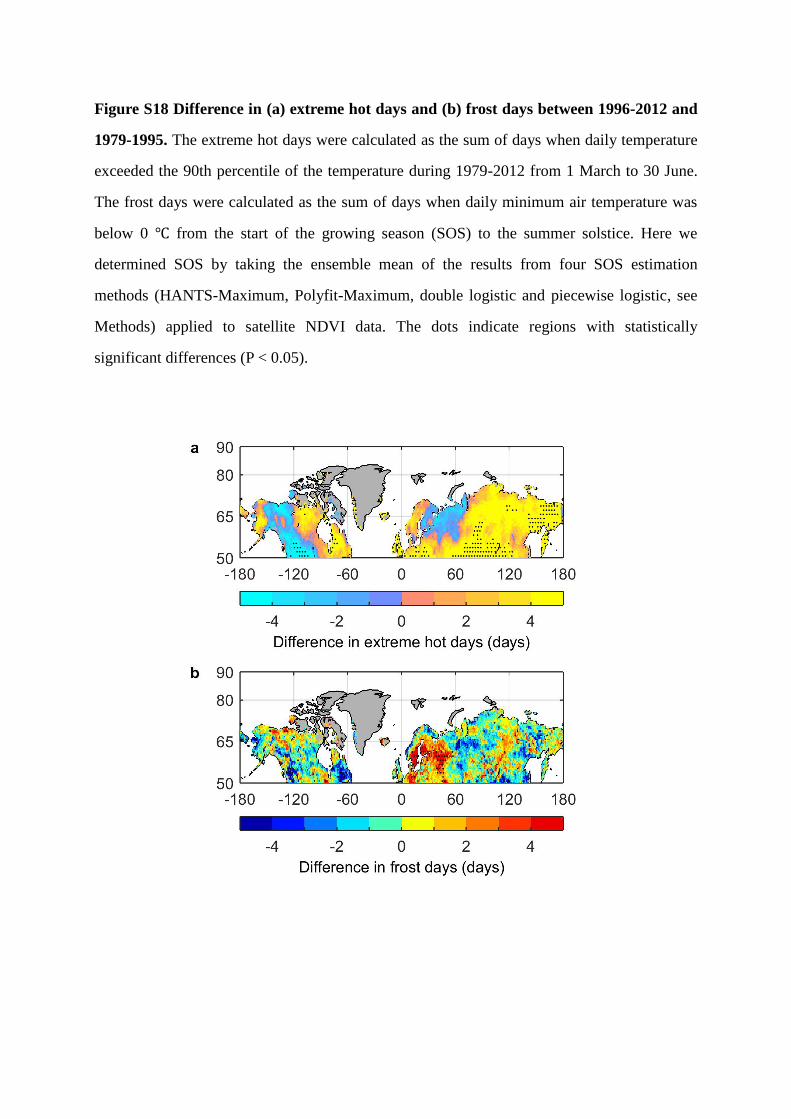
Figure S18 Difference in (a) extreme hot days and (b) frost days between 1996-2012 and

1979-1995. The extreme hot days were calculated as the sum of days when daily temperature

exceeded the 90th percentile of the temperature during 1979-2012 from 1 March to 30 June.

The frost days were calculated as the sum of days when daily minimum air temperature was

below 0 ℃ from the start of the growing season (SOS) to the summer solstice. Here we

determined SOS by taking the ensemble mean of the results from four SOS estimation

methods (HANTS-Maximum, Polyfit-Maximum, double logistic and piecewise logistic, see

Methods) applied to satellite NDVI data. The dots indicate regions with statistically

significant differences (P < 0.05).

Figure S19 Spatial distribution of (a and b) the mean green-up onset dates and (c and d)

trends in vegetation green-up dates during 1979-2012. The ORCHIDEE model-derived

results are shown in a and c, and the satellite-derived results are shown in b and d. The

modelled spring green-up date was estimated based on the seasonal cycle of simulated leaf

area index (LAI) following the approach developed by ref31. The observed spring green-up

date was obtained by taking the ensemble mean of the four estimation methods

(HANTS-Maximum, Polyfit-Maximum, double logistic and piecewise logistic, see Methods)

applied to satellite NDVI data. In the ORCHIDEE simulation, atmospheric CO2 and all

historical climate factors are changed. Note that the satellite data are only available from 1982

to 2011.

Figure S20 Same as Figure 2, but with no variables detrended.

Figure S21 The standard deviation (sd) of (a) SZC, (b) SCC, (c) spring temperature (ST),

andthe partial correlation coefficient of (d) SZC and (e) SCC with ST during the first 17

years (1979-1995), the second 17 years (1996-2012) and the first 17 years excluding year

1990. All variables are detrended before the sd calculation and partial correlation analysis.

The uncertainty is given using 500 bootstrap estimates.