Embed Size (px)
Citation preview

I! IIIIIIIIIIIIIIIIIIII
THiE INTEGRATION OF A HIGH VOLTAGE CABLE FAULTlOCATION INSTRUMENT WiTH
MODIERN INFORMATION TECHNOLOGY
BYROGIEIRJAMES xsu, Y
Dissertation submitted in compliance with the requirements for Master'sDegree in Technology in the Department of Electrical IEngineering(light Current)
at the Durban Institute of Technology
APPROVED FOIRFINAL SUBMISSION
l;/gfoLDate /fessor Vladimir B . c, D. IEng.Sc(E.E)
Supervisor

IIIIIIIIIIIIIIIIIIIII
Contents
1. Introduction
1.1Overview
1.2 Motivation
1.3 Research Goals and Scope
2. Introduction to Cable Fault Location by use of the Time
Domain Reflection (TDR) Method
2.1Time Domain Reflection Test Method for Fault Location
2.1.1 Cable Characteristic Impedance
2.1.2 Reflector Factor
2.1.3 Cable Attenuation/Loss
2.1.4 Velocity Factor
2.2Applications and High Voltage Derivatives and Methods
2.2.1 TDR Method
2.2.2 High Voltage Reflection Methods
2.2.2.1 High Voltage Surge Method
2.2.2.2 Discharge Pulse Detection Method
2.2.3 Pulse and High Voltage Generators
2.2.4 Coupling Methods
2.3Survey of the classic TDR instruments and the transition
to the Baseline approach
3. Baseline Approach Design
3.1Concept
3.2 Hardware
3.2.1 Bandwidth and Analogue Amplifier Requirements
3.2.1.1 The Amplifier/Attenuator Input Sections
3.2.2 High Speed Analogue to Digital Converter
2
8
8
9
10
14
14
15
16
16
17
19
19
21
22
23
25
26
26
28
28
28
29
32
32

IIIIIIIIIIIIIIIIIIIII
3.2.3 Data Collection Buffer as a Function of Cable 37Length and Resolution.
3.2.4Function/Pulse Generator and Cable Matching 40Considerations
3.2.4.1 Function Generator Pulse Width Range 403.2.5Triggering Considerations 42
3.2.5.1 Triggering Under Transient Capture 42
3.2.5.2Triggering under the TDR Type Cable 42Fault Location
3.2.6 Computing Platform and Data Controller Requirements 43
3.3 Software 443.3.1The Application Program Philosophy of the System 44
3.3.2 The Operating System 45
3.3.3 The Display 473.3.4 The Control Functions 51
3.3.5 The Data File/Storage Facility 523.3.6 Data Enhancing through Digital Signal Processing 533.3.7Database Fundamentals, Concepts and Programs 58
4. BaselineImplementation 62
4.1 Test Cases/Examples 624.1.1 High Voltage and Transient Operations 62
4.1.2 TDR and Related Low Voltage Methods 654.1.3 Refinements to Input Amplifier 66
4;1.4 Examples of Locating Complex Faults 68
4.2 Various Additional Applications and Refinements 70
4.2.1 Live Cables and Blocking Filters 704.2.2 Spin off Application 72
4.2.2.1 Remote Testing via Modem 73
4.2.2.2 Training Facilities 73
3

IIIIIIIIIIIIIIIIIIII
4.2.2.3 Database of Cables and Historic Databases
5. Implementation Results
5.1 Advantages
5.2 Disadvantages/Shortfalls
6. Conclusions and!Areas for Improvement and Refinement
7. Bibliography
4
73
75
75
76
77
79

III
Llst of lFiglUlres
I 2-1 Open Circuit 172-2 Short Circuit 17
I 2-3 Complex TOR WaveformlTrace 202-4 Multi "T" Domestic Cable Layout and its TOR pulse Response 21
I 2-5 High Voltage Storage Test Method 222-6 Traveling Surge Position Verse Time Diagram 22
I 2-7 Discharge Detection Test Method 23
2-8 Discharge Pulse Position Verse Time Diagram 24
I 2-9 The Arc Reflection Test Method 24
2-10 Superimposed Traces as seen by the Arc Reflection Method 25
I 3-1 Characteristic impedance and phase angle vs frequency 30
I of 25 - kV XLPE insulated power cable (Bartnikas et al. 2000)
3-2 Characteristic impedance and phase angle vs frequency 30
Iof coaxial polyethylene insulated communication cable
(Type RG - 58 ) (Bartnikas et al. 2000)
3-3 Attenuation vs frequency of 800 - ft 25 - kV XLPE power 30
I cable terminated with its approximate characteristic impedance
of 37 ohms (Bartnikas et al. 2000)
I 3-4 A 350 ps Rise/Fall time 10V Pulse monitored 36
on a 1 Ghz Sampling Oscilloscope. Direct 50W input
I connection is used (Williams 1993)
3-5 The test pulse appears smaller and slower on a 350 36
I Mhz instrument (t, = 1 ns ) (Williams 1993)
3-6 General arrangement of counters, AID converter and memory 38
I 3-7 The pulse generator block diagram 41
3-8 The Global Window, Expanded Window and Parameter 48
I Window of the Baseline screen
3-9 The Window Cursors or Markers on the Baseline Screen 48
II 5
II

IIII 3-10
3-11
I 3-123-13
I 3-14
3-15
I 4-1
I 4-2
4-3
I 4-4
4-5
I 4-64-7
I 4-8
4-9
IIIIIIIIII
A typical Baseline screen, including parameter details 49Measurement cursors and markers 49
Cable length parameters 50
An example of the magnification window 50
A further example of the magnification window 51A typical Baseline database record 60
A recall of an historic ICE trace 63
A typical ICE trace/waveform as viewed on the screen 64
Demonstration of the 'loop on loop off I method as used on a 64
short test cableA TDR trace without signal processing and correction 65
High speed TDR and data capture unit 67
Example of a complex fault 68The expanded close-in range TDR trace of a cable 69
Blocking filter schematic 71
Effects of a blocking filter on a TOR trace 72
6

IIIIIIIIIIIIIIIIIIIII
list of Tables
3-1 The attenuation at various frequencies for Cat 5 UTP cables
3-2 Recorded length for 4 Kbytes memory at two different
velocity factors3-3 Resolution in meters for various pulse widths
31
39
41
7

IIIIIIIIIIIIIIIIIIII
1.1 OvellVoew
Modern society as a whole seems destined to have an ever-increasing demand for
power for both industrial and domestic use, as continued population growth means
that cities, suburbs and industrial areas become larger and denser. At the same time
the trend toward increased productivity in all segments of industry is influencing the
development and techniques employed at locating faults in power cables and
networks to ensure only limited downtime and reduced direct and indirect costs
associated with the location of faults.
Although telecommunications are moving into the field of microwave and fibre optics,
power systems will remain on wire systems. Power distribution systems employ both
overhead lines/cables as well as underground cables. In order to keep pace with
expectations for increased power and efficient fault location it has been necessary for
cables and power transmission equipment, as well as techniques and methodologies
for identifying faults, to evolve so as to meet these demands and remain abreast with
the overall advancement in technology.
This thesis focuses on power cable fault location with an emphasis on the specific
area of cable fault location by the Time Domain Reflection (TOR) method. Derivatives
applicable in high voltage applications will also be addressed (Clegg et al. 1975 and
Gale 1975). There are several methods of fault location on power cable, as can be
found in references such as those by Tanaka et al. (1983), as well as Clegg (1995).
These various methods will be explored with the objective of building the case for an
8

IIIIIIIIIIIIIIIIIIII
integrated cable fault and cable reticulation database system, which will be describedin some detail in the body of this thesis.
1.2 Motovation
During a series of interviews and site visits in 1993 repeated complaints were
recorded by engineers involved in the location of cable faults as to the difficultiesfaced in locating pilot cable faults accurately. This difficulty on pilot cables is
essentially due to the noisy electrical environment, the length of cables and their
joints, which are at times approximately every 500 meters. Coupled to this is the fact
that TDR waveforms depicted on cable fault location instruments are often complex
and therefore not always straightforward to interpret making the fault location on pilotcables extremely difficult.
As most traditional cable fault location instruments at the time (1993) only capturedthe current TDR waveforms of the cable being explored, it became apparent that if a
method could be derived whereby an instrument could store TDR waveformscaptured before the fault, then this could be retrieved at the time a new fault was
being investigated, providing a comparison with the original, healthy TDR trace and
faCilitating in the interpretation as to the location of the fault. Considerations such as
aging, temperature etc. would however also need to be considered in this analysis.
By reviewing the literature on signal processing (Van Biesen et al. 1990 and Ho et al
1993), the probability of developing an instrument with these characteristics became
increasingly feasible. At the time (1993) fault location instruments did not have very
flexible storage functionality and usually made a hard copy of the waveform using aprinter or a Polaroid camera. In order to test the signal processing algorithms, abetter storage system and a platform, which would provide a lot of flexibility, was
needed. The personal computer provided the initial solution as data could becaptured via a high-speed data capture unit, saved and the results then processedand analysed. The next steps were therefore to define the goals and limitations and to
9

IIIIIIIIIIIIIIIIIIII
build the new instrument. This commenced in 1994 with on-going enhancements witheach test phase.
While this thesis will focus on the design, principals and methodologies of the original
instrument and the results captured, the concluding chapter will highlight the various
strengths and weaknesses that have become apparent through its implementation
and sets the conclusions/foundations as to the characteristics that will need to beincorporated into a new instrument, considering not only the observed strengths and
weaknesses but also the most recent advance in technology, drawing inter alia from
the paper "Signature Representation of Underground Cables and its Application to
Fault Diagnosis" by Ho et al. 1993, which has provided further validation to theproposed new instrument and its future enhancements.
1.3 Research GOC3l~S and Scope
The problem of fault location on wire cable belongs to several broad areas, namely to
Radio (Bisset 1988), Telephone, Communication and Power Engineering. Theparticular section that this research will be aimed at is power cables .as covered byClegg (1995) and McAlister (1982). Power wire networks can again be subdivided
into three subgroups namely High Voltage (HV), Low Voltage (LV) and Protection
System Networks. Although fault location methods could apply to all three subgroups
of networks, the main focus will be biased towards the fault location on protection
networks.
In power reticulation systems there are a number of substations feeding energy/power
into the network. Separate cables (pilot cables) link substations. These cables carrythe interconnected protection system signals. In the event that a fault develops in the
reticulation system the substations effected will transmit alarm and protection signalsto appropriately isolate them from. delivering energy to the fault. Without these
protection systems the cables and related equipment would be damaged due to the
10

IIIIIIIIIIIIIIIIIIIII
high levels of fault current. The protection system therefore forms an extremely vital
part of the reticulation system as do the pilot cables carrying the alarm control signals
for the protection systems.
One of the methods used for cable fault location is known as Time Domain Reflection
(TDR). Time Domain Reflection is also known as Pulse Echo (PE) and 'Radar
Method' as detailed in Clegg (1995). It is obtained by injecting a narrow pulse signal
into the one end of a cable and collecting the signal 'reflected' by the impedance
changes along the length of the cable. The cables are however not communication
cables and they are not terminated by the characteristic impedance of the cable. A
TDR trace therefore has many impedance mismatches caused by the joints along the
length of the cable. An occurrence of a fault adds additional 'mismatches' which may
indicate the position of the fault. The identification of the fault is therefore difficult due
to the abnormalities mentioned above and is compounded by the noise that is usually
present on such cables. There is also supporting evidence that a pulse applied to a
cable will cause a TDR trace that will be dependent on the cables topology. This
trace is repeatable and hence may be characterised as a 'Cable Signature' (Ho et al.
1993). The comparison of the cable's signature and the fault condition signature
should enable easier fault location. This is of great significance and supports the
justification of a database of 'signatures'. The database of signatures by itself is
however not of much use if the information is:-
not correctly collected
not always collected
difficult to use and apply
costly to apply in terms of additional overheads
or if the database management is not transparent to the fault location
engineer
While today's TDR type instruments are optimised for communication cable type
faults (Bisset 1988) they fall short in the number of traces that they can display and
11
IIIIIIIIIIIIIIIIIIII
information that can be managed for use at a later date. In short, they are goodinstruments but what is required is an integrated fault system. It is with this in mindand taking into account the significant advances in computer and informationtechnology that it was proposed to combine both these components to form anintegrated system placing more emphases on the system to enable rapid andaccurate fault location but on power pilot cables.
By actually producing a limited scale system (the Baseline) and evaluating it, will
produce evidence of the advantages of the proposed solution and will quantify thebenefits of such a systems. The proposed system is seen to considerably improve
fault location technology in the field of its application.
The research goals therefore focused on.-
• The development of a fault location instruments which will be controlled bya laptop computer
• The development of a methodology for establishing a system approach tofault location within an electrical distribution/utility company conditions
• Software development for implementation of the control, capture and
database program• The study and evaluation of the practical implementation of the system
evaluating the benefits
The challenges of the research can essentially be described as:-
• The development of an effective data capture instrument for capturing theTime Domain Reflection traces (hardware and software)
• The development of a storage/file manipulation system
• The development of a database• The development of a methodology for a comprehensive fault location
system developed for power transmission networks, specifically related to
12
IIIIIIIIIIIIIIIIIIII
the pilot cable fault location
The hypothesis around which the high speed cable fault location instrument
(Baseline) was developed was that the TDR trace obtained from a cable will indicatethe characteristic impedances changes along the cable length. This will characterize
the cable condition. By comparing the previous captured trace with that of onecaptured at the present time on the same cable will indicate changes due todegradation of the cable. A fault condition will be an extreme case and should
immediately flag the fault position in most cases.
13
IIIIIIIIIIIIIIIIIIIII
lntroductlon to Cable Fault Locatlon by use of the TomeDomain lRef~ection{TDR} Method
In this chapter the principles of the time domain reflection test methods used tolocate faults will be summarised, in particular the faults on power reticulation cablesystems and related cables.
2.1 Tome Domain Reflection Test Method! for Fault location
The time domain reflection method of locating faults in cables is based ontransmission line theory where a narrow pulse is injected into one end of the cableunder test. The transmitted pulse and its reflections, due to mismatches (impedancechanges) along the cable, are recorded and displayed on a display device such as a
crt ,video or Icd display.
Understanding just how the pulse will react with various types of impedance
mismatches allows the engineer to determine if a cable fault is either a short, open or
a high resistance fault. By knowing the time from the transmitted pulse to the returnpulse, as well as the velocity of propagation, the distance to the fault may be derived
from:
td=pc'2 where
t = time to fault and back
c = the speed of light ( m/s)
p = the velocity factor
While this forms the basis of the method, to obtain a clearer understanding a little
( 2.1)
14

IIIIIIIIIIIIIIIIIIIII
more detail needs to be explained.
2.1.1 Cable Characteristic Impedance
In a cable the conductors are separated by an insulation medium such as paper, oilimpregnated paper and, in newer cables, polymers as well as various pvc's. A cable
has a capacitance between conductors and possesses inductance and resistance. Todirect current (DC) the cable will be dominated by resistance. As the frequency isincreased the inductance and capacitance become increasingly more significant and
an approximation would need to include inductance and capacitance. At very high
frequencies the inductance and capacitance tend to be the dominant factors and thecable can be considered as a transmission line. At these frequencies the cable can beconsidered under transmission line theory. As such the cable will be seen to havean impedance which is termed the Characteristic Impedance (Millman et al. 1965)
where
Z = {Lo C
Zo = characteristic impedance
(2.2)which is given by
L = inductance
C = capacitance
The capacitance and inductance of the cable will be determined by the cable'sphysical construction. Factors such as conductor spacing and permittivity of theinsulating medium, termed cable construction geometry, affect the characteristic
impedance. As a result any change in the geometry of construction or change in theinsulating medium will result in a change in the characteristic impedance.
From transmission line theory (Millman et al. 1965) a transmission line terminated in
15

IIIIIIIIIIIIIIIIIIII
its characteristic impedance will not produce any reflections. From this it is inferred
that any line not terminated in its characteristic impedance will produce reflections. A
fault on a cable would usually alter the geometry of the cable at the point of fault and
hence a reflection would take place.
2.1.2 Reflection Factor
The reflection factor is the ratio of signal reflected and is given by:-
(2/20-1) .p= (2/20+ 1) (Millman et al. 1965) (2.3)
where Z is the termination impedance and Zo is the characteristic impedance
p is the reflection factor and has a value in the range - 1 to + 1
In general then if Z > Zo then p is positive which implies a non inverted reflected
waveform and if Z < Zo then p is negative which implies an inverted reflected
waveform.
It can further be inferred that
p = + 1
P = - 11 > P > 0-1 < P < 0
p = 0
=> Z is 00 or an open circuit
=> Z is 0 or a short circuit
=> Z > Ze=> Z < Zo=> Z = Zo
2.1.3 Cable Attenuation/loss
In addition to the reflection factor, cables do have losses which attenuate the injected
pulse. Thus a pulse injected into an open circuit cable is attenuated and reflected. If
16

IIIII
the pulse is attenuated by 10 dB while traveling to the end then the reflected pulse will
be subjected to a 10 dB attenuation. On arrival back at the input end it will be
attenuated by 20 dB and as the reflection factor is +1 from above it will not be
inverted.
II
An example of a pulse applied to an open or high resistance fault will produce a
waveform or trace as in Figure 2-1, while a pulse applied to a cable terminated in a
short will produce a waveform/trace as can be seen in Figure 2-2.
III Time Time
I Figure 2-1 Open Circuit Figure 2-2 Short Circuit
III
These waveforms, which are typical of this method will in future be referred to as a
Time Domain Reflection ( TDR) trace or waveform or more often just as a TDR trace.
2.1.4 Velocity Factor
II
Earlier it was stated that the distance to the fault could be obtained from the
expression:-
td=pc-2
(2.4)
I Firstly, as the pulse travels to the cable end and back it actually covers twice the
distance and thus must be divided by 2. Secondly, the velocity factor needs to be
II
17
II

IIIIIIIIIIIIIIIIIIIII
known in order for the distance to be accurately measured.
Once again from transmission theory (Millman et al 1965), for lines that are of
uniform cross section and in free space the velocity is given by:--
u = 1 1.JLC = f;€ (2.5)
where J1 = usu, and E = EOEr
J1 = 4 P x 10.7 which is the permittivity of free space.
E = 1/(36p x 109) which is the permeability free space.
For air the expression resolves to 3 x 10⁸ m/s or the speed of light ( c ).
For a dielectric the relative permittivity will be > 1, thus it is clear that the velocity of
the pulse in the cable will be traveling slower than the speed of light. The expression
(2.5) may be re written to take this into account as:
1u =
~(J1oEOEr)
~(J1oEo)
~(J1oEo€J
1p=--(~)
(2.6)
The velocity factor is given byu
r = =c
(2.7)
also sinceup=-c
it follows thatcu=--
~(€r)(2.6)
The above section provides the background and mechanism of the TDR method. The
principles also apply to various derived methods used in fault location on high voltage
cables which will be discussed later.
18

IIIIIIIIIIIIIIIIIIIII
2.2 AIPIP~DCaituOU1lSand IHUgh Vo~tatge lDell"DVaituves and Methods
While Chapter 2.1 described the principles and formula of the TOR method, thissection provides a very brief overview of the application of the principles and methodsand its directives as applicable in high voltage fault location. This is not a detaileddescription but rather gives an appreciation of the methods that are applicable. It isrelevant in the design phase of the hardware as well as software of the cable faultlocation instrument that was developed and is discussed later in this thesis. There are
many good references for a more detailed description such Clegg (1995), Millman etal. (1965), Dixon (1993) and William (1993).
2.2.1 TDR Method!
This method is also referred to as the "Low Voltage Pulse Radar Method" or "PulseEcho Method". While in a signal transmission cable every effort is made to match the
characteristic impedance of one cable to another at joins so as to minimize reflectionsthis is not the object for power cables and pilot cables. The main objective of power
cables is to deliver power at 50 or 60 Hz and as such a good connection andinsulation are the prime considerations.
In order to achieve these cable lengths many shorter lengths of cable are joinedtogether. As these cable lengths are usually set at the time that the cable is installed,
each section of cable will typically be the length that fits on a cable drum. Theselengths naturally vary for the thickness of cable and the drum size. The result of this isthat pilot cables might be joined every 500m and 11 kv three phase power cable at250m. Because the emphasis is on jointing the cable, as opposed to matching,
there will be significant reflections from both joints and terminations.
19

IIIIIIIIIIIIIIIIIIIII
When this method is applied to a pilot cable the complex TOR trace of Figure 2-3 is
more likely to be the result than that of the simple cable as shown in Figure 2-1 and
Figure 2-2 earlier.
.,The TOR trace shown in Figure 2-3 is that of a healthy pair in a 14 km cable.
Time
Figure 2-3: Complex TOR WaveformlTrace
From Figure 2-3 it will be seen that there are a vast number of reflections which give
rise to huge reflections at the beginning and diminish with cable length. The
transmission pulse experiences not only attenuation from the cable but each reflected
pulse is subjected to mismatches on the return path. This significantly attenuates the
return signal so making faults on long cables even more difficult to diagnose.
The TOR method is often applied to cables that have a main cable into which a
tapping is made to supply a user. The cable layout of such a network can be seen in
Figure 2-4. The application of a pulse injected into such a network will result in a TOR
trace as shown in Figure 2-4. Here again the reflections seen clearly show the joints
and terminations at the consumers. On closer inspection it is again noted that without
a cable layout drawing it is hard to distinguish which return pulse is the result of a
mismatch at the consumer or is due to a 'T'section.
As we are dealing with cable faults on high voltage cables, there are a number of
20

IIIII
methods that have the same principles of the TDR method but involve high voltagepulses.
III
Cable LayoutA
9~~--,rB
~ "-...... ... .....I .. '~..... ~, .., ...
I.
c
s
Eo...I - •
D
.......,
...,'\,,
II
DoD I
I
r I
I----'v- -XI
TimeTDR pulse response for pulse injected at S
Figure 2-4: Multi "T" Domestic Cable Layout and its TDR pulse Response
IIIII
2.2.2 High Voltage Reflection Methods
In high voltage networks a fault may flash over at the rated voltage which will causethe network to trip out by blowing a fuse or causing an electrical breaker to open. The
flash over may not cause the cable to be blown apart or become welded together. If
after a fault and circuit/network being isolated it can happen that the resistancebetween corresponding phases and earth shows no sign of a fault when tested. Onreconnection of the high voltage supply this will however once again result in a faultcondition. This is due to the ionization which takes place at the fault point as a resultof the high voltage being re-applied. The ionization results in an arc developing and
as this arc is a relatively low impedance path, high fault current results. These are
termed flashing faults. A low voltage TDR instrument may also not show much as thecables may not be damaged enough to show a massive reflection. Due to this,
methods have been developed over the years to apply high voltage pulses to thecable and record the reflections produced as a result. A very brief overview follows
IIII 21
II

IIII
2.2.2.1 High Voltage Surge Method
IThis method is also referred to as the "High Voltage Pulse Radar Method" (Tanaka1983). The high voltage developed is rectified and charges up a capacitor to a set
voltage. Once this voltage is reached a switch is closed and the high voltage pulseapplied to the cable under test is as in Figure 2-5:I
I
II
x-_-
24~ Surge Generator1 _
II
Figure 2-5: High Voltage Storage Test Method
Surge Input
Time
IIII
Figure 2-6: Traveling Surge Position Verse Time Diagram
IThe main difference is that the high voltage pulse behaves in the first instant just likethe low voltage TDR, however at some time later ionization takes place and at thatinstant the impedance at the point of fault drops to a low value. The result is that afterionization the high voltage pulse travels only to the point of fault and back. Thisoscillation continues until the energy has been dissipated as a result of the cableI
II 22
II

IIIIIIIII
losses. The main distinction is that there is an ionization time to take into
consideration.
2.2.2.2 Discharge Pulse Detection Method
This method is also known as the "Discharge Detection Pulse Radar Method" (Tanaka
1983) as well as the 'Relaxation Test' (Clegg 1995) and is demonstrated in Figure 2-7
below:-
IIII
24~ ~rge Generator .1 :
Kv
t
Figure 2-7: Discharge Detection Test Method
If a high voltage pulse is injected into the cable under test and the fault (high
impedance) does not ionize then the pulse simply travels to the end and back and
continues this oscillation as it is attenuated by the losses in the cable. This does not
give a fault position but simply provides the length of the cable.
III
In order to cause the fault point to ionize and arc/ flash over the cable is charged up
to the required test voltage and kept there until ionization takes place so causing a
flash over. This flash over produces a low impedance path and the cable is rapidly
discharged. This discharging generates a wave traveling in both directions away from
the fault and again oscillating until the energy has been dissipated. The wave
traveling in the section connected to the fault recorder travels repeatedly between the
fault and the recording end. This is depicted in Figure 2-8.
II,III
Figure 2-8: Discharge Pulse Position Verse Time Diagram
23
\

III
Sur gel n p u [ X
II Fa u I [ Po in [
I Tim e
II
If= (P2Ct) xxxxIt can thus be seen that the distance to the fault is given by
I II
A combination of the TDR and Discharge Pulse Detection Method or Relaxation Testis termed the "Arc Reflection Method" (Clegg 1995) and the 'Modified Pulse Radar
Measurement Method" (Tanaka 1983). This is illustrated in Figure 2-9.
I: ••.•••••••.•..•• : X'-T-· .· .· .· .· .
I240V: Surge Generator
-1- :
II
D o o
Figure 2-9: The Arc Reflection Test Method
I
In this method a generator that generates high voltage DC is applied to the cable
under test. A TDR instrument is coupled to the cable under test as well via a high
pass filter, which is also capable of withstanding the high voltage DC. The TDRcaptures a trace of the cable before the high voltage is applied. Next the high voltage
is applied causing the fault to ionize and an arc to form. Another TDR trace is thencaptured. The two traces are then superimposed as indicated in Figure 2-10. From
the first and second traces the divergence indicates the point of fault. This is found by
II
II 24
I

IIIIIIIIIIIIIIIIIIII
the equation (2.1).
""0a~ I----...J«
Open end
1 Fault point
Tim e
Figure 2-10: Superimposed Traces as seen by the Arc Reflection Method
As illustrated above, there are a number of TDR methods for which the applications
and high voltage derivatives share the same principles.
Section 2.1 and 2.2 of this chapter have provided an overview of some of the
considerations when desiqnlnq an instrument for the waveform analysis as applicable
in the field of power cable fault location. The next section considers the way in which
the coupling is made to cables especially at high voltages and introduces the coupler.
2.2.3 Pulse and High Voltage Generators
It is necessary to include the differences between pulse generators for low voltage
and high voltage in order to understand the waveforms that appear later.
The low voltage type pulse generators produce a pulse that is essentially a fixed
voltage and usually less than 10v peak. These pulse generators usually have the
ability to vary the pulse width from around 10 ns to 200 ns. The pulse is usually of
positive polarity and the rise and fall times are usually in the order of 5 ns to 20 ns.
25

IIII
High voltage pulse generators in contrast are usually referred to as surge generators
and basically consist of a high voltage transformer, the output of which is rectified and
fed to a capacitor or capacitor bank. The capacitor bank is charged negatively and the
voltage is usually controlled by varying the primary voltage, either electronically or
very often by a variac. The pulse is simply generated by closing a switch which then
applies the charge on the capacitor to the cable. Thus on the high voltage traces
shown the generator pulse appears as being negative.
IIIIII
2.2.4 Coupling Methods
Applying the TDR signal to the cable is quite simple but at high voltages this poses
problems. The method of coupling to a high voltage cable can be done by a divider
circuit. This is usually done by making use of capacitor divider's. The difficulty in terms
of the high voltage and in achieving a high frequency response is often considerable.
I An easier connection was developed by Gale (1975) in which a linear coupler was
used in the return or ground path of the surge generator.
III
2.3 SlUIrveyof the classic TDR instruments and the transition to
the Baseline approach
I
As mentioned in section 2.1 of this chapter the instruments that were around when
the Baseline cable fault location instrument was conceptualised where relatively
unsophisticated and had limited function digital oscilloscopes. The classic instruments
that had more than one channel where largely being replaced by the newer digital
oscilloscopes. The digital memories could save a waveform but many where not
capable of retaining these when switched off. If a waveform was required for storage
it had to be either photographed or, on the newer digital scopes, it could be printed.
II
III
26

IIIIIIIIIIIIIIIIIIII
As mentioned these were oscilloscopes and the most advanced TOR and cable fault
transient recorders had just reached the digital stage. The use of digital memories has
a major advantage as a TOR trace of a healthy pair can be compared with the faulty
one. Comparing the difference will normally indicate the point of fault.
Apart from the pilot cable fault location problems there are many instances where the
engineer would like a comparative trace. This led to the idea that in addition to being
able to save the data for processing it could also be used as a reference should the
same cable develop a fault in the future. A non-damaged saved TOR trace could
therefore be considered as a baseline from which to start. A paper published by Ho et
al. (1993) "Signature Representation of Underground Cables and its Application to
Cable Fault Diagnosis" considers that the TOR trace can be viewed as a signature
representation which characterizes the cable length giving further weight to the
original idea behind the Baseline instrument, which combines a personal computer
and a high speed transient data capture unit.
The next chapter focuses on the bandwidth and analogue amplifier requirements for
the Baseline instrument.
27

IIIIIIIIIIIIIIIIIIIII
Chapter 3
3.1 Concept
While the concept and theoretical framework for the Baseline instrument have briefly
been described in the overview section and in various parts of Chapter 2, this chapter
will focus on the various considerations and conclusions reached in the design of the
hardware and the software.
3.2 Hardware
The Baseline data capture instrument was designed to perform two types of test
functions, namely:-
o Transient capture on power fault locations and
o Time domain reflection waveform capturing
Although there are only two broad categories of tests on the cables as listed above
some additional parameters needed to be considered in order to understand/define
the constraints of the instrument, while simultaneously delivering meaningful results.
These parameters will be described in greater details in the remainder of this chapter.
Apart from the physical limitations that exist in the hardware and software, there are
also cost/benefit considerations that would influence the design of an instrument. For
the purposes of this paper, limited focus will however be placed on these
considerations.
28

IIIIIIIIIIIIIIIIIIII
3.2.1 Bandwidth and Analogue Amplifier Requirements
One of the first considerations was to understand the impedances that the instrumentmight have to encounter. It can be seen from Clegg (1995) that for a 0.6/1.0 kVbelted cable with 4 cores the characteristic impedance ranges from 12.0 - 18.2 ohms,
while 11 kV three core cable ranges from 18 ~ to 27.0 ohms. With a twisted pair
cable, as in pilot wires the characteristic impedance is around 90 to 100 ohm. Theimpedance range spans 12 to 100 ohms.
An additional consideration in the understanding of the required parameters is thebandwidth of the cable. As the two main areas that the instrument was designed to
be used in were fault location on power cables and pilot cables a consideration ofthese frequency responses was also be necessary.
Firstly considering a 25 kV XLPE cable and referring to Figure 3-1 and Figure 3-2(Bartnikas et al. 2000) it was noted that the characteristic impedance variedenormously from a minimum value of 50 ohms to 250 - a range of 200 ohms.Bartnikas et al. (2000) sited this to be the 'semiconducting shields' which causes thecable to behave as a complex quantity.
Also it can be seen from the attenuation versus frequency plot in Figure 2-14 that the
attenuation for this cable was approximately -40 dB and at greater frequencies on
average, the attenuation was around this figure.
Included for comparison from the Bartnikas et al. (2000) is the test conducted on a
RG 58 communication cable. This shows that the characteristic impedance range is
44 to 55, which is a total deviation of 11 ohms across the test frequency.
29

IIII t~O
JOIJ
5 :::'il)
~ .:!U<.r! l:rd',.!Oi In...Ii'....!:t ()}
-lOll
-1;'1)10011:
-41:>
Ju
'"-·::r,·~-410 ~~
&1'.I
I'
I , ·l.U'
I------r-~----..._----'-_.__----;:...-____l-t"';·:!G"-~·
F~~'
I Figure 3-1: Characteristic impedance and phase angle vs frequency of 25 - kV XLPE insulated
power cable (Bartnikaset al. 2000)
IIII ."~+----_---"'-------'----~-"'"'I"'~~--------!J"".
ILl2Plr.: ::l>l!.11Il:r
"'r:a'~!
IFigure 3-2: Characteristic impedance and phase angle vs frequency of coaxial polyethylene
insulated communication cable (Type RG - 58 ) (Bartnikaset al. 2000)
III
'0<;,1
I Figure 3-3: Attenuation vs frequency of 800 - ft 25 - kV XLPE power cable terminated with its
approximate characteristic impedance of 37 ohms (Bartnikaset al. 2000)
IFor the twisted pair similar to the pilot cable, a Cat 5 UTP solid cable, which is actually
II 30
II
IIIIII
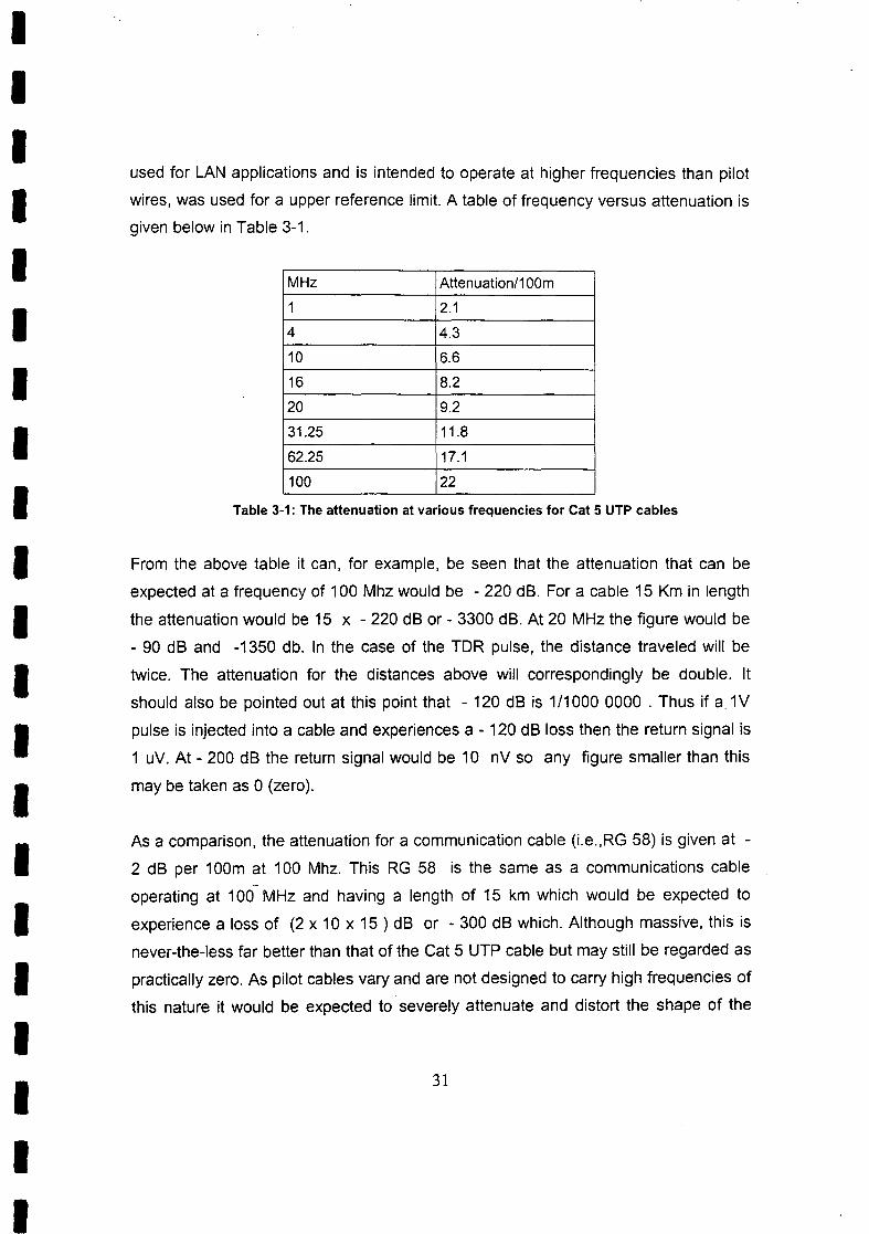
used for LAN applications and is intended to operate at higher frequencies than pilotwires, was used for a upper reference limit. A table of frequency versus attenuation isgiven below in Table 3-1.
III
MHz Attenuation/100m
1 2.1
4 4.3
10 6.6
16 8.2
20 9.2
31.25 11.8
62.25 17.1
100 22
Table 3-1: The attenuation at various frequencies for Cat 5 UTP cables
IIIII
From the above table it can, for example, be seen that the attenuation that can beexpected at a frequency of 100 Mhz would be - 220 dB. For a cable 15 Km in length
the attenuation would be 15 x - 220 dB or - 3300 dB. At 20 MHz the figure would be- 90 dB and -1350 db. In the case of the TOR pulse, the distance traveled will be
twice. The attenuation for the distances above will correspondingly be double. Itshould also be pointed out at this point that - 120 dB is 1/1000 0000 . Thus if a 1V
pulse is injected into a cable and experiences a - 120 dB loss then the return signal is1 uV. At - 200 dB the return signal would be 10 nV so any figure smaller than this
may be taken as 0 (zero).
II
As a comparison, the attenuation for a communication cable (Le.,RG 58) is given at -2 dB per 100m at 100 Mhz. This RG 58 is the same as a communications cable
operating at 100 MHz and having a length of 15 km which would be expected toexperience a loss of (2 x 10 x 15 ) dB or - 300 dB which. Although massive, this is
never-the-Iess far better than that of the Cat 5 UTP cable but may still be regarded aspractically zero. As pilot cables vary and are not designed to carry high frequencies ofthis nature it would be expected to severely attenuate and distort the shape of the
III 31
II

IIIIIIIIIIIIIIIIIIIII
injected pulse.
Each of these factors had to be taken into consideration when designing the entire
circuitry and demonstrate some of the potential difficulties or constraints.
3.2.1.1 The Ampiifier/Attenuator Input Sections
Given the above parameters it was decided to have two amplifier/attenuator sections
in the Baseline instrument; one for the transient capture mode to be used in
conjunction with the high voltage fault location. The second amplifier would be
coupled to the pulse generator for the TDR cable fault location. These separate inputs
would be selectable via a selection switch on the instrument's front panel.
Considering the substantial attenuation above 20 Mhz, and that for the XLPE cable at
frequencies greater than this the average attenuation appeared to be in the order of
- 50 db, a bandwidth of 80 Mhz was deemed to be appropriate. With this, the input
section would mean that all frequencies up to 40 Mhz would only be affected by a
loss of 1 dB.
3.2.2 High Speed Analogue to Digital Converter
When determining which analogue to digital (AID) converter to use for the Baseline it
was concluded that a flash 8 bit AID converter with sample and hold and a bandwidth
of 30 MHz was the most appropriate. The choice of the appropriate AID converter was
influenced by what components were readily available at the time of design and the
various considerations described below.
Firstly, under transient operation the instrument would be in use to locate high-voltage
faults. Under these circumstances the pulse or traveling wave oscillates between the
pulse injected end of the cable (input) and the end until ionisation takes place, at
32

IIIIIIIIIIIIIIII
which point the traveling wave travels between the input and the flashover point,
which is the point of fault. The distance to the fault is calculated using the formula: -
(3.1 )
40 m samples per second gives a sampling interval of 25 ns. By substituting this value
for time gives the resolution that can be expected. For a XLPE power cable the
velocity factor would be around 0.65. The resolution could be expressed as:-
d = (O.63x3xl08 x25 xIO-9)
r 2 (3.2)
=> dr=2.36 [m]
This implies that in the best case faults can be located to within 2.36 m. The error this
represents on a 1 km cable is 0.263% error. It is generally stated that as a rule of
thumb a distance of 1% on either side of the fault should be searched (Millman et
al.1965) and so the above error due to resolution is deemed to be acceptable.
III
The second consideration is whether the AID for the transient capture would be
acceptable for the TDR functions. When reviewing TDR reflections with regards to
the bandwidth of the AID converter the limitations set by the cable under test also
need to be considered. As already mentioned the pilot wires are only designed to
carry signal frequencies in the order of kHz. Frequencies in the MHz range are not
considered. Due to this and the fact that there are many various cables used for pilot
wires, each with their own bandwidth characteristics, a cable with superior frequency
responses was selected for reference comparison. On cables in real-life situations it
would be expected that the bandwidth could be worse.
33
II

IIIIIIIIIIIIIIIIIIIII
For the data/waveform capture an open circuit or short circuit would be visually
detected and the fault point would be resolved within the previous stated 2.36m.
Another point to consider was whether information other than an open circuit or short
circuit would be detected to enable more subtle influences to be visibly seen. If the
amplifier section can be considered a high resistance input section, with some strong
capacitance shunting this to ground, followed by an ideal amp, then this input section
can be considered an RC circuit and as such will have a rise time associated with the
RC time constant.
Applying a pulse to such a circuit results in a rise time which can be expressed in the
equation (3.3) below by considering the definition of rise time, as the time taken for a
signal to rise from 10% to 90% of its final value.
(3.3)
For a RC type circuit this can then be expressed as:-
jt=O.35where f = frequency
t = rise time (10% - 90%)
(3.4)
If the upper frequency f can be considered as the bandwidth frequency the equation
can be rewritten as follows:-
(3.5)
34

IIIIIIIIIIIIIIIIIIIII
=> t =0.35r BW
BW= 0.35t,
and
For the AID converter a rise time will be seen to be:-
0.35t=---r (35XI06)
= 10 ns
Only considering the AID converter it can be inferred that if the capture
signal/waveform rise time is slower than that of the AID converter then the AID
converter should be able to follow the signal with a limited distortion. If the captured
signal has a rise time faster than that of the AID converter then it can be assumed
that there will be a distortion as the AID converter cannot follow the input waveform
response.
Assuming that one might want to inject pulses with a 5 ns rise time into the cable
under test there would be both distortion and attenuation. The bandwidth for this rise
time would from the previous equations, be calculated as:-
BW= 0.35sx 10-9
=> 70 MHz
As this is one octave it would be expected that the attenuation would be -6 dB.
However due to the fact that the waveform is decaying exponentially this takes time.
For a pulse with a amplitude of V the decay is given by:-
-I
V = Verco
(3.6)
35

IIIIIIIIIIIIIIIIIIIII
The waveform is therefore not only attenuated but appears to have a wider pulsewidth due to the exponential decay.
An application note titled 'High Speed Amplifier Techniques by Williams (1993) gives
some clues as to what can be expected. In the section that deals with oscilloscopesand oscilloscope probes a good example of using a lower bandwidth oscilloscope isgiven. The pulse as shown in Figure 3-4 is 1 ns in pulse width, as well as having a10 V peak. Of interest is that with a 350 MHz bandwidth oscilloscope the original
waveform is attenuated and very slightly distorted but shows a good resemblance to
the original pulse.
Figure 3-4:A 350 ps Rise/Fall time 10V Pulse monitored on a 1 Ghz Sampling Oscilloscope.
Direct 50W input connection is used (William 1993)
Figure 3-5: The test pulse appears smaller and slower on a 350 Mhz instrument (t, = 1 ns )
(Williams 1993)
36

IIIIIIIIIIIIIIIIIIIII
From this it can be inferred that signals close to 2.86 times bandwidth can still bereadily observed and in the case of the AID converter's track-and-hold amp shouldstill give a reasonable result if it can be arranged by interleaving. For the 35 MHzbandwidth of the AID's track-and-hold amp a signal that has a frequency of 35 x 2.86or 100.1 MHz should be able to be captured, albeit attenuated and slightly distorted.
This demonstrates that in examining the waveforms of a TDR trace, the shape of thewaveforms is more important than the amplitude. Therefore the use of the 40 mega
samples/second AID converter with a bandwidth [of 35 MHz) would be acceptable if
the slight limitations are taken into account.
This AID converter would have a frequency response that at 70 MHz would be -6 dB.Looking at the Table 3-1 for Cat 5 UTP solid cable it can be seen that at a frequencyof 62.25 MHz the attenuation per 100m would be >17.1 db. Thus at these
frequencies and as the pulsed travels 2 x length (to end and back) this gives anattenuation > -342 dB /km . Cable lengths of 5 to 10 km are very common so theattenuation for a 5 km cable (> -1710 dB) is far in excess of the 6 dB loss in the AIDand shows that the limitation is cable rather than the instrument let alone the AID
converter.
3.2.3 Data Collection Buffer as a Function of Cable length and!
Resolution
In Chapter 3.2.2 it was shown that the resolution that could be expected at a velocityfactor of 0.63 would be 2.36 m. Sampling at 40 mega samples per second with a
memory depth of 1K bytes (1024) gives a TDR or 'trace distance' of 2.3 x 1024 or
2355 m per Kbytes of memory.
A more general expression can be developed as follows:-
37

IIII
frompets
dr=-2-
IIII
where R I = Recorded trace distance
p = velocity factor
c = speed of light
T s = sampling period
Md = Memory depth or size
I 1as T =f R, can be expressed in terms of sampling frequency:-
II
peMdR,= (3.7)z j,
I As a 4 Kbytes (4096) memory was available at the time and addressing could be
carried out using 12 bits this conveniently could be done by using 3 cascaded, 4 bit
counters. The general arrangement is shown in Figure 3-6 below.III
I
.----------------------------I~~~~I ~
I -1·
IFigure 3-6 General arrangement of counters, AID converter and memory
II 38
II

IIIIII Recorded Recorded
Frequency r1 Distance @r1 r2 Distance @r2
o MHz 0.63 9674 0.7 10749
20 MHz 0.63 19349 0.7 21499
10 MHz 0.63 38698 0.7 42998
5 MHz 0.63 77398 0.7 85995
2.5 MHz 0.63 154791 0.7 171990
III Table 3-2: Recorded length for 4 Kbytes memory at two different velocity factors
I For a sampling frequency of 40 Mhz, a velocity factor of 0.63 and with a resolution of
2.3 m the accuracy would be :-
I~XI00 %9674
II
=> 0.024%
I The above results are more than adequate for sampling purposes. There were
however two additional reasons for using the 4 Kbytes of memory at the time. These
where:-II i. As the data/transient capture unit was to be a separate unit the data would
have to be passed to the Personal Computer (PC) where it could be
displayed, processed and saved. As the connection would be a RS232
serial type, depending on the data and operation being performed, thisII
-
would take more time for more data. The latent time from triggering the unit
I 39
II
IIII
till the data (waveforms) would be displayed was considered and kept to a
minimum.
Iii. The storage would be on floppy disks and with 4 Kbytes of data per trace
this meant that if no other data was to be saved then 64 TOR/transient
traces/waveforms could be stored on a disk. If data was also to be saved
then at least 40 to 50 traces could be saved.II 3.2.4 Function/Pulse Gel11erator and Cable MatchliB1lgOonslderatlons
I As the TOR requires that a pulse is injected into the cable under test and the resulting
waveform captured, an appropriate pulse generator needed to be integrated into the
unit for the TOR functions of the unit. This was to incorporate a variable pulse width.
In addition, due to the attenuation mentioned earlier, as well as the noise from cross
talk on the pilot wire cables, it was decided to also include a variable amplitude
capability.
IIII
3.2.4. ~ FIUIB1Ictioll1Generator Pulse Width and Amplitude Range
II
The determination of the function generator range was the next problem that needed
to be resolved. Consulting Dixon (1993) provided a good rule of thumb - i.e., 'The
resolution obtained along the length (of cable) is approximately one-tenth of the
wavelength of the frequency corresponding to the rise time'.
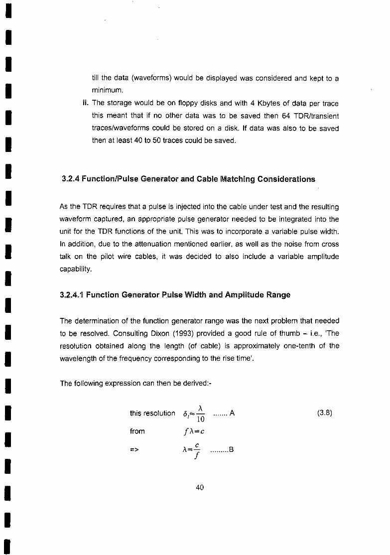
I The following expression can then be derived:-
I this resolution,\
....... A (3.8)8 R::-I 10
from f,\=c
c .........8=> ,\=-f
III 40
II

IIII substituting B into A gives
c8~-- CI 10j .
I As the speed in a cable is slower, the velocity is v= pc
IFor a cable the expression C can be written as
pc8~--I 10JI
IThe resolution can readily be tabulated for various frequencies as follows:
IFrequencies p=l p=0.83 p=0.63Mhz m m m
20 1.5 0.83 0.63
50 0.9 1.25 0.95
100 0.27 0.75 0.57
200 0.04 0.22 0.17
III
Table 3-3: Resolution in meters for various pulse widths
The design parameters for the pulse width generator were set as follows :-
II
Minimum pulse width
Maximum pulse width
Min Amplitude
Maximum Amplitude
5 ns
10 ms
3 Volts
25 Volts
I Designing the pulse generator in order to obtain a high slew rate, as well as a variable
amplitude pulse was not trivial. While compromises had to be made, the required
results were achieved as will be seen later in the example TOR traces. Figure 3-7
outlines the general block diagram of the pulse generator configuration.
IIII 41
I

IIII
I
Vs = 3...27V
r-,Pulse Enabl Pulse Generator Buffe
Pulse outputat TTL Levels Level Impedance Matchin
Trans tor
V~;, ;, ;,
I
IFigure 3·7: The pulse generator block diagram
III
3.2.5 TriggeriD1lg Consideratlcns
A method for capturing data in the TOR unit needed to be initiated, recognizing thatthe method differs for the transient capture and TOR functions. These two methodsare outlined below.
I 3.2.5. ~ Triggering Under Transient Captaue
I
I
Triggering under transient capture is related to the data to be captured during a highvoltage fault location using a surge generator. Under these conditions the highvoltage pulse is applied to the cable and travels to the cable end and back until
ionization takes place, at which point the travel is to the point of fault and back. Thetime to ionize is the critical element and as this does not occur within a defined time
the data capture needs to be initiated at the start of the high voltage pulse injection.The triggering therefore needs to be level and directionally sensitive and as such is
asynchronous just as an oscilloscope.
II
II
3.2.5.2 Triggering under the TDR Type Cable Fault location
IFor the TOR fault location there is no ionization time so the best method is to trigger
III
42

IIIII
off the pulse enable signal so making the triggering synchronous. This method allows
data to be collected and post processing or signal processing to be easily carried out.
One of the major errors to be concerned with is jitter that would be introduced by the
high speed data capture itself. As the order of magnitude is in the sub nano second
region, whereas the data that is to be captured is of a greater order of magnitude, the
effect of the jitter on the final results is deemed not to be material at this data capture
rate. Papers such as 'The Effects of Timing Jitter in Sampling Systems' (Souders et
al. 1990) and 'Effect of Sampling Jitter on Some Sine Wave Measurements' (Wagdy
et al. (1990) considers some of the effects of jitter.
IIIIIIIIIIIIIIII
3.2.6 Computing Platform and Data Controller Requirements
As the data/transient and pulse generator was to be a stand alone instrument all
communication was to take place with the personal computer via the RS232 serial
cable. There also had to be a microprocessor controlling the unit. The type of
microprocessor was not of much concern at that time. The main concern was that the
microprocessor would act as an instruction processor. This meant that it would have a
list of instructions to set up the data capture sections, such as the amplifier gains,
trigger settings as well as the trigger direction. The instruction would be issued from
the controlling Personal Computer (PC) which would do the signal processing as well
as displaying and managing of the data.
In order to ensure potability of the cable fault location instrument, a laptop PC, with an
Intel 80286 or 80386 processor was used. Other important features were that the PC
had to have a serial RS232 and printer port as well as a floppy disk drive. The initial
portable PC or laptop had a monochrome display, although a colour PC's soon
became the norm and replaced the monochrome version.
43

IIIIIIIIIIIIIIIIIIIII
3.3 Software
Chapter 3.2 has dealt with describing the hardware considerations and requirementsfor a fully integrated cable fault location system. The functionality of such a system is
however driven by the appropriate software or application programs. The variouscomponents to be considered in the software/application design of the end productare: --
• the application program philosophy of the system• the operating system
• the display
• the control functions
• data file/storage facility
3.2.1 TlheApplication Program Philosophy of the System
A PC has a number of programs that perform various functions. These programs arecalled application programs or just applications. The processor is therefore an
application that performs the task of writing documents. The personal computer (PC)
is normally supplied with a few of these application programs namely notepads, word
processors, databases, spreadsheets as well as organisers. In order to be able tocollect, save and view the data collected by the high-speed transient recorder it is
necessary to have an application program to provide this function. To create aprogram, a theme or philosophy has to be followed with the objective of reaching the
desired goal.
The philosophy or theme that was initially followed for the experimental researchinstrument was to have a small number of application programs each performing afunction. Collectively these application programs would deliver the desired result orobjective. This approach benefits from the fact that a small application can easily
44

IIIIIIIIIIIIIIIIIIII
accept configuration changes. The software for each of these applications therefore
needs to be written in a highly modular way thereby facilitating changes. At the
system level small stand-alone applications that can be scheduled in and out at will
are also beneficial. This arrangement also allows for rapid changes and tests.
For a dedicated instrument to be used by an operator the applications need to be
more automated and system details more transparent to the operator. The functions
need to be more rigid and integrated into the system.
3.3.2 The Operating System
The main objectives of an operating system, which runs application programs that
control the separate high-speed data recorder are:-
• that the system should cater for serial communication ports
• the boot up time should be relatively quick and automatic
• it should be able to recover quickly to major disruptions e.g., as in the event
of a power failure
• the system can be multitasking but does not have to be totally deterministic
as these functions can be handled by the remote high-speed data recorder
• the system needs to be supported with a good set of tools for development
purposes
• documentation of the internal workings should readily be available
• the system should support all the modern storage mediums, such as, floppy
disks, CO-ROM's and hard drives
• a support for higher resolution graphic devices is essential
• upgrades to the system must be backward compatible
Originally the operating system was selected on other factors, namely that it was
freely available, open and supported IBM compatible PCs. Essentially the operating
45

IIIIIIIIIIIIIIIIIIII
system (DOS -- by Microsoft ) performed most of the functions listed above. Therewere however a few limitations, such as memory limits that needed to be considered.
Using the DOS operating system applications were relatively easily developed andcompatible with the early Windows operating systems. While later upgrades toWindows tended to result in improved graphics, the compatibility with the original
operating system became more complex and required consistentenhancements/upgrades to the application software.
While it is not the intention to discuss these compatibility problems in details there are
considerable drawbacks in using Windows systems for embedded or stand-aloneinstruments have become evident. For example, should an operator merely switch theinstrument off without shutting down, as required by Windows, there is the risk thatthe system can be corrupted. This therefore requires a potential change in thebehavior of the operator of the instrument as other electronic instruments, such as theoscilloscope are merely switched off, without requiring a lengthy "shutting down"
routine. Furthermore, when next operated it would be expected that as the instrumentwarms up it will be operating on the functions and parameters that were previously
selected. Lengthy start times as experienced with Windows operating applicationsalso leave a negative impression as engineers working with the instrument tend to be
impatient and wish to get on with the task at hand. The operating system of aninstrument should therefore always be transparent to the operator, which is not the
case when using a Windows based system.
In a DOS based system if the power was removed at the next start-up of the
instrument it would simply go ahead with the application polnted to in the batch files.One may have lost the data collected at the time but the system would largely have
remained stable.
46

IIIIIIIIIIIIIIIIIIIII
3.3.3 The Display
When the first proto-type of the instrument was developed the graphics user interface
(GUI) was not available which meant that the graphical displays had to be manually
programmed.
When designing a graphical interface it is important to create an effective
environment that is intuitive to use. An effective display in a cable fault location
instrument is one that focuses the attention on the desired detail results while
simultaneously providing a broad overview. This is the philosophy that was applied to
the Baseline application software.
One of the main considerations regarding the waveforms was to be able to display all
required information on the screen without loslnq the necessary level of detail. The
information that needed to be displayed was:-
o the waveform data for the cable length under view/test.
o a section of detail which could magnify a desired portion of the waveform
and
o a section to show the parameters in use such as velocity factor, distance
etc
The solution that was developed and is described below is illustrated by snapshots
taken from the final screen designs.
Displaying a 13 to 15 TDR trace results in a great variation in the waveforms. In this
waveform there is usually a small area of interest. The ability to zoom into a particular
section meant that a magnification function was required, bearing in mind that the
operator of the instrument should also be able to see the entire waveform displayed.
This was achieved by segmenting the screen into three views as shown in Figure 3-8
to Figure 3-14.
47

IIIIIIIIIIIIIIIIIIIII
• View 1 known as 'the global window' was to hold the entire length of theTOR trace of the cable under test
• View 2 known as 'the zoom or expanded window' enlarged and focused inon the particular section defined by the window cursers set in the globalview.
• View 3 known as 'the parameters windows' held the parameterscorresponding to the settings of the instrument such as gain, triggering
parameters, printer and distance between the measuring cursers,calculated as the velocity factor.
-1'------- --p~WLnOO\1,
Figure 3-8: The Global Window, Expanded Window and Parameter Window of the Baseline screen
!be ~"'i:mdowClJ.Ti.Im or~
Figure 3-9: The Windows Cursors or Markers on the Baseline Screen
48

IIIIIIIIII Time
Figure 3-10: A typical Baseline screen, including parameter details
III
---~. _ .__~J"" .
_,- -- _,,- . ~,.1-- I V ,
_r"
, ..~/
i _,.
!/./,/ J..v,,,,,,
i "J I.p,c,,..~--;
! ,// I!;II
II .../I
iIII -
IIII
Figure 3-11: Measurement Cursors and Markers
II 49
II
~...wl~ Lon '" Iii.:- : Ira •
il':-CJ>404i6t~,.. u-61.:..c.:..l"6-(l r ru~o: }
1D.lh b t.fII9WSC..;> t .. :
bil:iit) O_l
I-V. 11"1 ': ....
t;.1P L..... ,,!
I;,TIll:; N\T ~ 'tD~-~~"€e1) (~tP.- ('1~'11'5: is tl~I'
-;0. G.2olc;ul~1tC Lho:: dios.1on"" lie·
':til: PO_L oJ IUlt=rt ~nllllll);.r;>iI·~ L.~ LllfQ ~c·!iO~

IIII
.> •• d. :4 1n'~lu,~.e:!l::.lO'tlPIC:
I,'-'_ ..,
IIII
Time
I Figure 3-14: An further example of the magnification window
I3.3.4 The Control IFUJW1CtioD1s
II
With any control function the layout should be as simple and intuitive as possible. As
the control of the data capture instrument (Baseline) was to be conducted from the
laptop computer a few options were available. These included the use of:-
I • Keys or keyboard• Mouse or roller ball.• Graphics pad or tablet
• Touch screen
IIII
As the instrument was designed to be portable and for use in the field to collect data
one of the concerns was the operating environment in which the fault location would
be conducted. Usually this operation would be from a test van or in a substation.These environments are usually dusty and present a number of problems to the
above devices. The keyboard was considered the device least affected under these
II 51
II

IIIIIIIIIIIIIIIIIIIII
conditions. On first impression function keys and using keys in general seemed a little
awkward. However, tests showed that when the instrument was in constant use -
usually daily - it did not take long for the operator to become accustomed to the
functions associated with the keys. Once the operator has reached this stage,
conducting or performing an operation was rapid and possibly faster than using one
of the pointing devices such as a mouse.
One exception to this is in selecting a section of the waveform to be magnified. While
this operation is presently done with keys, using one of the more modern pointing
devices such as an infrared tracker-ball would possibly improve this greatly in terms of
speed. These new infrared track-balls, although not as yet tested would probably
also be able to withstand the dusty conditions in which the instrument would be used.
3.3.5 The Data lFile/Storage Facility
One of the main features that distinguish this instrument/system from the previous
generation instruments is the ability to save data and related information in a coherent
format. This data can either be saved onto the:-
o internal hard drive or
o a floppy disk drivelCD Rom
Apart from just saving the waveform data, information regarding the saved waveform,
as seen in Figure 3-10, can also be stored for later retrieval and post processing, for
example:-
o the instrument's operational parameters such as sampling speed and
velocity of propagation
o a data file consisting of comments and circuit descriptions relating to the
waveform being saved.
52

IIIII
The data storage functionalities are the instrument's and in fact the system's biggestadvantages as it enables original data to be recalled while examining a new fault. Byrecalling not only the waveform but also related data and superimposing the newwaveform reading on the original trace the fault diagnostic is facilitated. Not only does
the waveform provide a reference but the original related notes also provide thenecessary background, such as:-I
II
• the cable length• the propagation velocity• the cable'end would have been established and so that becomes known
• mismatches form a signature which is characteristic of the cable or pilot wireunder examination and so the 'historic signature' is known
• when a comparison of another new trace is made with the historic signaturea great difference usually occurs at the fault point
IIIIII
3.3.6 Data Enhancing through Digital Signal Processing
As was seen earlier the longer the cable, the greater the attenuation of the injected
signal. The higher the frequency the higher the loss. Therefore for a pulse with a 1ns rise time injected into a cable, which is terminated in an open circuit there is a
reflected pulse which is not only attenuated but will be seen to have a longer rise
time.
I By fourier analysis a pulse waveform can be shown to consist of a fundamental
frequency and harmonics. Any periodic function may be expressed as a fourier
series:-III
(3.9)
III
53

IIIIII
where
2 f i'I tt ta;=y: f(t)cos--y;-dl where i=O,1,2, ....
where i=1,2, ....
IIIIII
and T= period of f(t) where T=}
If the injected pulse is repeated then the reflected waveform will be classed as aperiodic function. From this it can be seen that the higher frequency components of ainjected pulse (into a cable), together with the reflected resultant waveform, areattenuated with the even more attenuated higher harmonics. The result of this is thata pulse injected with a fast rise time returns with a slower rise time and appearsrounded. The longer the cable the more the attenuation, the slower rise time and
greater 'rounding' of the pulse corners. This phenomenon severely effects the test
engineer as will be explained below.
IIIII
When interpreting the reflected waveformlTDR trace the engineer is looking for
reflected pulses. The start of the pulse indicates the location of the feature thatcaused that disturbance and may well be the fault position. If the cable is long thestart of a pulse is however well rounded making the identification of the start pointdifficult. This problem is known and methods have been developed to try to improve
the accuracy. As described later this was addressed by an algorithm which effectively
magnified the event and by so doing made the transition more visible. The derived
algorithm described below will illustrate this.
IIII
One of the major problems which in fact motivated the development of this instrument
was the noise encountered on pilot wires. As noise is a random event a process of
54

IIIIIIIIIIIIIIIIIIII
cumulative averaging can reduce the noise. The first constraint however is that thesignal needs to be repetitive and to remove the random data sampling there needs tobe a means to synchronise the data capture event. In order to do this the datacapture was initiated by using a trigger supplied directly from the pulse generator. Tothe extent that the waveforms are individual data points, which are summed and then
accumulated, while the noise is random and limited to its peak value, then the signalwill increase relative to the noise. If expressed in terms of power, as noise generallyis, then the expression for Signal to Noise Ratio (SNR) from Horowitz et al (1982) will
be given by :-
PsSNR=1010g-Pn
(3.10)
where Psis the signal power
P n is the noise power
An error that is also curnulative through this method is DC offsets. These are usuallyare small and can be removed by signal processing. This is very easily accomplishedby automatically disconnecting the cable and sampling without generating a pulse,
followed by either averaging or filtering. This will ensure that only the DC offset
remains and any spurious noise is removed . This can be achieved with either amoving average filter, as described by the expression below (Smith 1997) or by
accumulative averaging as expressed in the formula above :-
(3-11)
The DC offset is then subtracted from each individual point. This can be expressed
as:-
55

IIIIIIIIIIIIIIIIIIIII
Yi=Xi-ede for i = 1 to n (n = 4096) (3-12)
where n = the number of data points collected (in this case 4096)
Y i is the sample without DC offset
Xi is the sample including the DC offset
ede is the DC offset
Once the DC offset has been removed the noise can be reduced by cumulativeaveraging.
The specific method that was implemented in the Baseline instrument was a
derivative of the method described above as it was decided, as far as possible, towork with integer math in both calculations and display functions.
Firstly a waveform/trace was captured and saved in an array. This was repeatedseveral time and added to the array. Next the resultant accumulative data was divided
by the number of waveforms captured, which gave the average. The result was savedto another array termed the Accumulated Array. As the above process was
repeated, subsequent results were summed. At the end the Summed Array was
averaged by dividing by the number of iterations performed. This was followed by
subtracting the DC offset multiplied by the number of secondary iterations. The result
of this was firstly noise reduction by averaging in the first stage and then accumulativeaveraging in the second stage, as well as any DC offset removal.
Putting this in mathematical terms is done as follows:-
Let the array of sampled data for the waveform of 4096 points be considered as an
Array of 1x4096 or a simply a vector S and considering that the DC offset can be
considered as an array filled with the DC offset error s;
56

III
Therefore if three waveforms Sp S2' S3 ,were taken then averaged this can be
Iwritten as a resultant vector (3.13)
II
Now assuming that the above entire process is repeated 4 times and added, then theOC error subtracted, the result can be expressed as:-
II
(3-14)
where SA would be the resultant vector.
II
A more general mathematical description for (3-13) and (3-14) above would be asfollows:-
I- 1 In -s =- Sm rn r=l
(3-15)
I(3-16)
III
As memory was however to be conserved in the Baseline, arrays were not
implemented in line with the described equations but rather followed the detailed
description above.
IHowever as the number of iterations completed by the first general equation (3-14) isIn' and by the second 'm' it can be seen that for the above where n = 3 and m = 4
would mean that 12 TOR traces would be captured and processed. Making n = 10and m = 10 then 100 TOR traces would be processed. By making these factorsadjustable in the Baseline application process the test engineer could change these
III 57
II

IIIIIIIIIIIIIIIIIIIII
factors until the desired averaging and cumulative sum was achieved. This methodwas used very successfully with positive results.
In general the approach has been to only implement algorithms that give exceptionalresults for all data collected and processed in commercial systems. The experimentalmachine (Baseline for development purposes) has other signal processing algorithms
that are undergoing a refinement process. One of the advantages of having the PCand operating system is that the process of experimenting with, and including, newalgorithms is greatly facilitated.
3.3.7 Database Fundamentals, Concepts and Programs
When data, in this case cable traces and related data, is being collected on a regular
basis at some point trying to keep all the information obtained and being able toreference back to a particular trace becomes difficult. Of benefit to the user wouldtherefore be a database/library where data can be 'looked up' and subsequentlyloaded into the memory for use and analytics. The ideal system for such purposes
would be a relational database which stores not only cable traces but all related
information required by the test engineer for easy access. This would, for exampleinclude, the substation location and equipment as well as cables and their routingmaps/charts. Building such a database is no small feat. A scaled-down version wastherefore designed with the main objective being able to see if there was a 'baseline'
trace for a particular cable and if so to display this historic information. As it wasenvisaged that changes would initially be made frequently to the system, the concept
was to separate the database function from the application program.
Using the high-speed data capture unit (Baseline), cable traces and information
collected during the location of cable faults was initially saved and filed on disc. Oncethe fault location process was completed then the files would be edited and anyadditional comments made in a standard template, using a file browse and edit
application program. The next stage was to run the database application program
58

IIIIIIIIIIIIIIIIIIIII
and load these new traces and data into the database as records. As the data for the
individual fields within a record were a function of the high-speed data application
program all the corresponding fields would be updated. The database fields that
were included are: --
• Date
• Time
• Substation ID
• Cable ID
• Engineer ID
• Contractor ID
• Jointer ID
• Trace Data
• Notes
• File Name
The primary key was chosen to be a combination of the date, time, substation 10, as
well as the cable ID which would make the record unique. This would allow one
record per second to be saved. It could have been arranged that each of the ID fields
such as 'Engineers ID' were foreign keys so making a relational database. This is
reserved for future enhancements. As such the 'Engineer ID' could have been linked
to engineers database which would have fields such as : --
• Engineers ID
• Surname
• First name
• Address
An example of the data stored in the database is illustrated in Figure 3-15 below.
59

IIIIIIIIIIIIIIIII
"~~--"""''''''''~~-----..---._..._.-.__
:JO'It,Qs~r.::ld.ll::>L l':ldlDH_oeo::.t.ionr Ad::trC33C.rC1.1::''!: HS~ Sta.t. IcnTrc;;r..sto:rI.18.l·· 7:-.(!,w i 1 r~'hCable
D1.::r:i m inqh·~1UviI:>!:: 007~';;
l...iOC". t: r;:r,ct: ex..iL){ .,~r. 1:'.1
Not';-e 11,Jot;. :.:r.t)1 r'! ..."
C~I>:. L""qtil.11 ~:1Il 1
---'''HI)~.'-D
[)~l' ~ L*tlCfthIS:' ( .. J
Ccnl•• la'''''9
P.C
r::tf,i ....ta ..1It-2 L..a.1NI P
A t.1.,dL..:t! ', ,( ,0::1' ~ 1 '.,.,_ r ~;:;r=?3 ll1<'ln::1::1g tne :!:ir~not;ic¢~lc ~~~~cpancyk !'·.Jrtller 200m. in of the t i.r et, e~ct.::.on
Figure 3-15: A typical database record
IIII
60

IIIIIIIIIIIIIIIIIIIII
While the initial foundations of a database were developed and supplied as astandard application with the Baseline instrument the concept and functionalities werenot fully developed given the considerable scope of such a project. As an interimstep, data was stored as a flat file for pure reference purposes without providing thebenefits to be had from a fully integrated relational database.
Unfortunately as the maintenance of the data records was viewed as an extra
'housekeeping' function, test engineers did not use this feature to its full extent.
Future developments will therefore need to not only focus on developing a more fully
integrated database but also ensure that the completion of all related data is easily
integrated into the test engineer's fault location processes.
61

IIIIIIIIIIIIIIIIIIIII
4.~ Test Cases/lExamlP~es
The previous chapters have dealt with the issues in the design of an instrument thatcould be capable of high-speed data capture, as well as the data processing and
filing. This section will provide a few examples of the various uses and also discusses
some of the changes and improvements to the system. Examples of traces used are
an exact replica of a trace on the screen of the PC or laptop at the time of the test.While on the screen these traces were in colour, thereby facilitating the analysis, thecopies used in this paper are black and white, which may therefore make the
illustration less effective.
Examples of tests described below can be divided into the High Voltage and
Transient method followed by the TOR and related low voltage methods.
4.1.1 High Voltage and Transient Operations
A few examples of various high voltage tests using a linear coupler and a test methodreferred to as the ICE (Gale 1975, Clegg 1995) method, as described in Chapter
2.2.4, are illustrated below.
In recalling an historic ICE trace the instrument would be set up according topreviously filed/stored traces and data. On observing the trace in Figure 4-1 together
with notes that may have been made at the time makes the test engineer more awareof what to expect. Although the new trace will not be the same, unless the fault is
62

III
exactly in the same place and ionisation takes place at precisely the same time, to the
trained eye a lot of information is already present. The distance/length will be valid, as
well as the first excursion time of the pulse to the cable end and back as ionisation
has not yet taken place. The above example would therefore be the starting point for
the location of a new fault on the same cable.
III
C"acbl ...... n<~"~!) It I.m :I
III
:7 L r Ifl 1
I --c:;, ...
~L.deitr- 1;;,·.11 nO<.j'z." [~. 1
II
~...
Time
II
Figure 4-1: A recall of a historic ICE trace
Another example is given in Figure 4-2. This is the typical display seen after capturing
an 'ICE' trace and shows the global window together with the magnified window and
parameters.IFigure 4-3 demonstrates another method namely the 'loop on loop off method, used
in conjunction with the 'ICE' test method. While this test was conducted on a short test
cable, it clearly demonstrates the results. Once again this method can be found in
various references such as that by Clegg (1995).
IIII 63
II
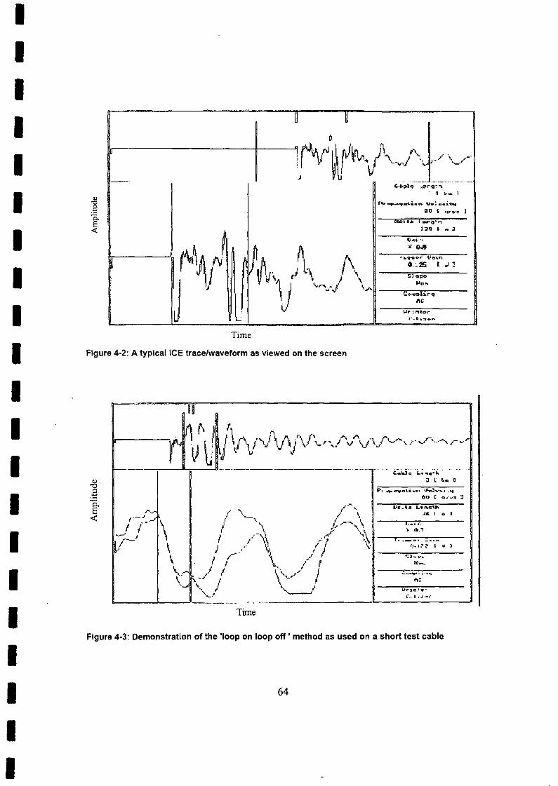
IIIIIIIIIIIIIIIIIIIII
B H
0
!r-v~\fln".!,--,J\v,J \J-- I V
---- J_ ...•.-.....-~.- ..... -..
If..g.jq ...pr-Q-:'"I ~.. I
It-. ~""'"'9crl.c.G_ lUao ~ '.. a a. ....
: ttQ I 1" WOO ~
ItD6:Ea.a 'I ~.., ..:'1I I'll I N l
rn~~j! 1i.;i· "I
J~if' ,;\:~ O,.I!I
-\ ""lII.q:-a.'" 11.: e.Ln
~ O.~2!'i 0 .J ~
l 1 : I
.I " ~J ~;:oi \
J ' V ....'ro,..~J \.... "'n',",
Lc~..,:::tl~,..q.
RC
...... "!".CU·
1:.1"3_'"
Time
Figure 4·2: A typical ICE trace/waveform as viewed on the screen
......_--___.--- ..-.~...- ._.- ..Time
Figure 4·3: Demonstration of the 'Ioop on loop off ' method as used on a short test cable
64

IIIII
4.1.2 TOR and Related low Voltage Methods
The TDR implementation function is illustrated in Figure 4-4 below. As demonstrated
this did not incorporate data processing such as cumulative averaging hence the
noise is present on the TDR trace. In a power environment this noise is ever present
especially when power consumption levels are high and as a result large currents are
involved. Cables are usually laid in ducts and trunks and therefore suffer noise from
cross talk. The method used to 'smooth out' this noise is cumulative averaging.
IIIIIIIIII
~6::>L.. Leon;h'" ( <D )
I"r ocolla !no QIJ'I. (iif,;tn.u .1 Gill r _ .•.•. 1
'Jill'"
,'h";';'''''· ~ ... r.u.uzu D U _
Figure 4-4: A TOR trace without signal processing and correction.
II
With cumulative averaging the noise is vastly reduced. Various algorithms were
tested and then given further field trials before they were incorporated in a function
which made the application (Baseline) runtime easy and intuitive, while the details and
complexity remained transparent to the operator.IIII
65
IIIIIIIIIIIIIIIIIIIII
4.1.3 Refinemelnts to the Input Amplifier
Tests on short and medium length cables (3 Km) showed that the TDR was morethan acceptable for this range however on testing longer cables and again long pilotcables the results were not acceptable. Beyond 5 km the details were not clear.
Increasing the pulse width and amplitude compounded the problem as it resulted in
'swamping' the input amplifier while still being unable to deal with the small returnsignals in the order of the millivolt range.
On examination of the problem it became clear that no digital processing would beable to improve the situation. When the amplifier reaches its limits:-
• any signal beyond the limit is irrelevant
the amplifier is no longer operating in the linear region but is rather
operating in the saturated or swamped region• the saturation region leads to the amplifier needing a recovery time. Even
though the signal amplitude may be within the amplifier range it is not
following and lags behind adding more waveform distortion.
The problem was tackled by reevaluating the specifications with the conclusion that
the new limit requirements should be:
Max. Pulse Amplitude : 25V
Min Pulse Amplitude : mV
The voltage ran.~ewas therefore 25,000 millivolts.
This represents a range of 87.96 dB. An 8 bit AID converter can resolve 1 part in 256
also :-
i4=16384
i5=32768
66

IIIIIIIIIIIIIIIIIIIII
By observation of the above at least a 15 bit AID was required. As an 8 bit AID was
built into the instrument some type of compression needed to be incorporated. This
function could be accomplished by:-
o varying the attenuation or gain proportional to time
• using a limiting amplifier with a logarithmic function
By limiting the input signal at the start to +/- 1 V greatly improves the situation
especially if there is a logarithmic function involved.
Another factor that was considered was the fact that as a section of the cable was
being examined the pulse amplitude, as well as the pulse width, had to be set so as to
optimise the reflected pulse and waveform. The limiting amplifier was constructed and
bench tests were then conducted which showed that the amplifier was functioning as
expected. The block diagram in Figure 4-5 shows where the limiting amplifier was
introduced into the high speed data acquisition/capture instrument (Baseline). Field
tests were scheduled on a 15 km pilot cable and the results were very positive.
localControlProcessor
Serial CommsRS 232 link
High Speed TOR and Data Capture Unit
Figure 4-5: High speed TOR and data capture unit
67

IIIIIIIIIIIIIIIIIIIII
By adding further digital signal processing algorithms which could now deal with thesignal range a further enhancement was achieved. An example of the results with anamplifier can be seen in Chapter 4.1.4 under examples of locating complex faults.
While the system was operating well in the field trials it became apparent that other
areas could be explored. What follows is a very brief discussion of each of these
together with relevant data and captured waveforms.
4.1.4 Examples of Locating Complex Faults
As in the case of pilot cable faults mentioned in the introductory section in Chapter
2.2.1, comparative methods provide a significant aid in the location of faults on these
cables. The progress in colour display also meant that the system could be furtherenhanced to take advantage of the additional features and a multiple trace facilitywas added. A total of 4 traces could be viewed simultaneously by this method. Theability to display multiple traces each in a different colour facilitated the process of
identifying major differences, which would correspondingly be the probable point of
fault. An example of this are shown in Figure 4-6 and Figure 4-7.
-....... Ii '" _
- •.••-------~----~--~---I1;.!;!I11I11tZ. \.crf'"llllil"h
1, I: C "~. :)
1).,.1 .... ~9u",d
'.I- 1:'.... t n. ::I
C..unJ.. I....~
..."" .. ,...... ,..
TimeFigure 4-6: Example of a complex fault
68

IIIII
Figure 4-6 illustrates a typical TOR waveform/trace taken on a pilot cable. The global
window is set up to show an 11 km cable length at a velocity factor of O.64c (thespeed of light). As this velocity factor is adjusted to give the correct length of thecable it is an average value and as such is a nominally set factor. This is referred toas ~ nominally velocity of propagation factor or NVP in the parameter window.
I In the zoomed or expanded window the trace from the global screen, as well as apreviously saved trace, which was stored in one of the memories, can be displayed.
This is illustrated in Figure 4-7 below.II -.
I~
f~~""''''' ......_,----_......_/-~---... ...... ----
~C 01:1.. _''''~t-
_1 I ..'" )
~u...-H ( _D 1.
. 1\ ~ O'ltL~:O L.Ift"lQt ...
\(I.• '" {'I\\ ~.~:t t • 1
!~ C"a';ll
~~~i'~j\'\L''-- -x :1.1
tM ~..~l!""". I \~\"\;ifI .. ,j .r-Ii! I
~I ~~ COiJ~'_L -e
~ito-
.1J ,I ' P,.ir.1",,'
B ,",po w....oor
IIIIIII
Time
I Figure 4-7: The expanded close-in range TOR trace of a cable
II
Any memory can be viewed or hidden at will allowing details to be removed or added
as required.
I 69
II

IIIIIIIIIIIIIIIIIIIII
As was seen and discussed earlier (Chapter 3) a drop off in signal amplitude with
distance/time was experienced. This is due to the attenuation discussed. The higher
attenuation or roll-off higher frequencies can also be easily depicted. The noise due to
cross talk was also severely reduced by signal processing, such that the noise was no
longer an issue.
When viewing Figure 4-6 and Figure 4-7 above it becomes apparent that the entire
cable would have to be examined to achieve effective results. This is done by
zooming into sections of the cable utilising the 'window cursor' control functions. It is
also clear that with complex waveforms, as shown, the comparative method facilitates
the process of locating cable faults. With only one TOR trace the task would be
almost impossible. A future development could make use of an algorithm to aid in the
location process purely on comparative bases on multiple traces.
4.2. Varlous Addltlonal AppHcations and Refinements
4.2.1 live Cables and Blocking filters
With power reticulation systems much of the distributed power is transformed down
from the kilovolt range into the 240 V to 380 V (UK) range for domestic and industrial
use.
Locating faults in the domestic and industrial voltage range usually involve the TOR
type tests. It is not always possible to isolate consumers and so high-voltage pulses
cannot be applied to the cable under diagnosis or test. Precautions are taken which
assume any cable to be worked on as live. If a TOR type instrument is attached to
these low voltage cables (low tension cables or LV cables) and the cable is energised,
apart from the engineer being hurt or potentially electrocuted, the instrument would
70

IIIIIIIIIII'IIIIIIIIII
also be destroyed. In order to facilitate this a blocking filter has to be inserted betweenthe instrument and the cable under investigation. The function of this blocking filter isto allow the narrow pulses to still be injected into the cable, while simultaneouslyblocking or isolating the 50 Hz mains. The blocking filter has to be fail-safe and, inthe event of catastrophic failure of the filter components, both the operator andinstrument must be totally safe.
As the emphasis is on safety while simultaneously delivering the pulses, a few
compromises had to be made in the design of the blocking filter. Figure 4-8 outlinesthe basic concept of the blocking filter.
Instrument Side Live Mains Side 110 - 380V
... - .. - - - ... - - - . - - - - . - - . - - - .. - . - - - ~
Figure 4-8: Blocking filter schematic
It must be noted that because of the high frequency nature of the pulses, the design
of the blocking filter needs to be suitable for frequencies in the 10 MHz to 200 MHz
range. The layout and components, including wound components, therefore need tobe considered and constructed for the rf. frequency spectrum. This means the
inductor needs to be a broad band bifilar winding, and core and capacitors need
careful consideration.
As mentioned earlier stray inductance and parasitic capacitance will introduce
distortion. If a blocking filter is used on very long LV cables then, due to the increased
pulse amplitude and pulse width, these small parasitic parameters start to become
Significant, with the result that they tend to become visible on the TOR trace. An
71
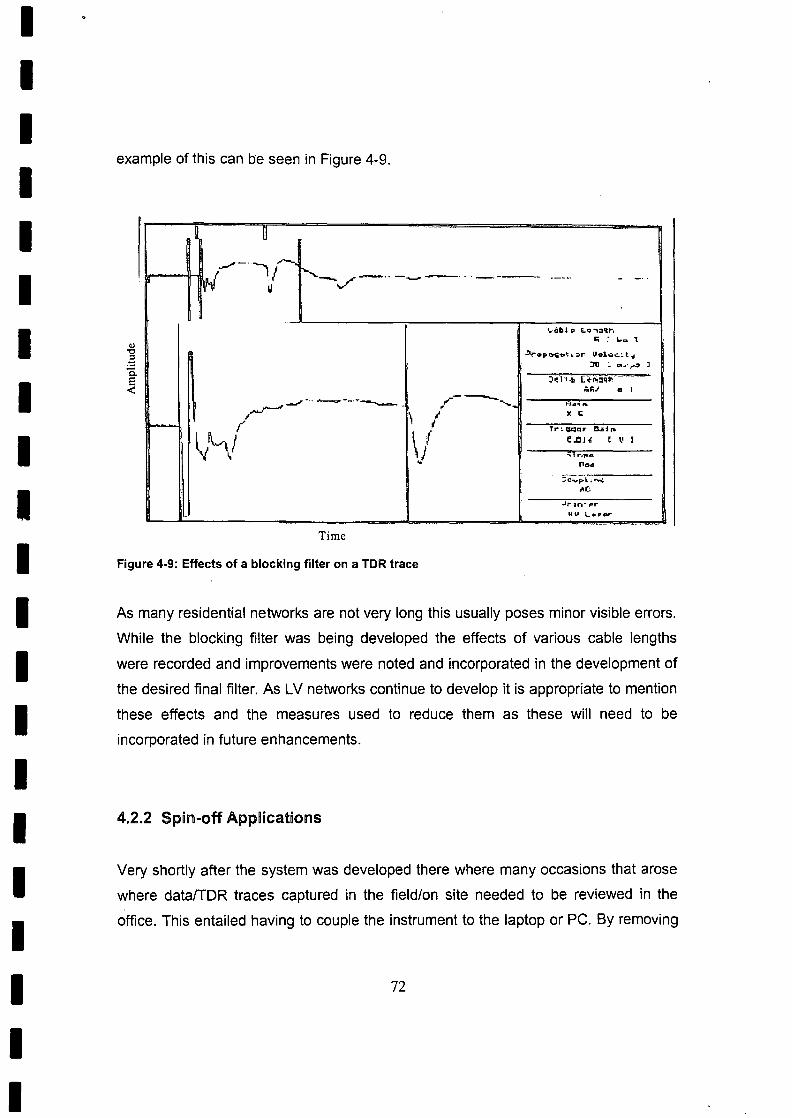
III
example of this can be seen in Figure 4-9.
IIII II)
"0
.€c..E«I
III
[ D
"'--"1"-"VJ" / "'--- ...,...-- .. _-_ ... _.---
Tr:.l;It1or l3..!ii ...
f.flH r \1 I
;-~~·L.""'i-It(:
UU L ...."..,.,.
Figure 4-9: Effects of a blocking filter on a TOR trace
Time
I As many residential networks are not very long this usually poses minor visible errors.
While the blocking filter was being developed the effects of various cable lengths
were recorded and improvements were noted and incorporated in the development of
the desired final filter. As LV networks continue to develop it is appropriate to mention
these effects and the measures used to reduce them as these will need to be
incorporated in future enhancements.
III
4.2.2 Spil1aoff ApplicationsII Very shortly after the system was developed there where many occasions that arose
where data/TDR traces captured in the field/on site needed to be reviewed in the
office. This entailed having to couple the instrument to the laptop or PC. By removingIIII
72

IIII
the initialising, control and data capturing routines from the initial application software
a virtual instrument was developed - termed the Baseline browser. This proved to be
a valuable additional functionality of the instrument, opening up more applications for
off-site viewing, even enabling traces to be e-mailed, viewed and printed remotely.III
4.2.2.1 Remote Testing via Modem
IAs the instrument is controlled via the serial port this means that introducing a modem
at either end allows the instrument section to be controlled over the phone line. This
feature has been tested between London and Edinburgh in Scotland (UK). From this
it is possible to infer that as long as the phone link is good this feature of remote
operation will be possible. With this facility it is conceivable that a specialist engineer
could have subordinate junior test engineers take permits and couple the instrument
and surge generators to the cable to be tested. Once each engineer had 'coupled up'
the specialist engineer could then take over and perform all the diagnosis and fault
location from a remote head office. Facilitating such a structure or hierarchy could
have significant cost and productivity benefits.
IIIII
4.2.2.2 Trainill1g Facttttles
IAs the Baseline browser allows waveforms and data files to be saved and retrieved,
waveforms captured during a large number of cable fault location exercises can be
saved and then used at a later date for teaching purposes.
II 4.2.2.3 Databases of Cables 31111d Historic Databases
III
In addition to storing individual traces in cesiqnated memories and files for future
retrieval, one of the key future enhancements of the Baseline system, as described in
Chapter 3.3.7 will be the development of database facilities which will, for example,
73
II

IIIIII,IIIIIIIIIIIIIII
enable utility companies to create a full and complete database of all cables in theareas for which they have responsibility. The task of capturing and storing cabletraces for existing cables is vast although it could be envisaged that in newlydeveloped areas this is undertaken as a matter of routine. For existing cables the
database could be built over time in that each time a fault is located the cable
concerned would automatically be stored in the database.
74

IIIIIIIIIIIIIIIIIIIII
The best way to analyse the results of the original objectives in the design of the
Baseline instrument can be summed up in terms of advantages and achievements, as
well as any disadvantages and shortfalls.
5.~ Advantages
When comparing the Baseline instrument with existing instruments, as well as viewing
the particular functionalities of the Baseline the advantages can be summarised as
follows:-
• The storage of waveforms and data has worked well
• The location of complex faults is greatly facilitated through colour screens
and the features that enable the comparison with previously stored traces.
This is particularly effective on pilot wire faults
• Signal processing has minimised the noise problem and with simultaneous
multi-trace viewing has made fault location easier
• Remote testing has become a possibility
• A virtual instrument means the training with real examples can be
undertaken
• Historical data filed can be retrieved
• Analysis and comparison can be undertaken off-site in a quiet un-
pressurised environment
• Application software can readily be upgraded
• Algorithms can be amended and directly incorporated into the application
75

IIIIIIIIIIIIIIIIIIIII
software
• From a development perspective, the instrument can act as a research
instrument in that it can be used to collect data to test new:-
~ algorithms for future use, including neural network algorithms
~ hardware designs and configurations so that new test results can be
compared with previous ones by observing the resulting waveforms
5.2 Disadvantages IShoirt1falls
As the Baseline database was not embedded in the system, the instrument has not
had a great take-up rate. This will therefore be an area for future development by
having a database that is an integral part of the data capture and control application.
76

IIIIIIIIIIIIIIIIIIIII
COIr1ChllSDIOIlil§ and A IT'Sa flOIT' Improvement callIild
Refunement
What this thesis has attempted to do is to not only provide the theoretical backgroundas to the various methods applied in the location of faults on underground cable butalso to describe how these methods and principles were applied to the design and
development of a high speed cable fault location instrument referred to as theBaseline. Through the development of this instrument a review was undertaken of
similar competitor instruments that existed at the time and while integrating most of
the features available in these instruments, the Baseline also introduce some newconcepts, such as PC based control, multi-trace visualisation, multi-colour traces,
remote operation and filing which facilitates historic data recall with automatic
instrument set-up.
As demonstrated with selected screen prints, considerable testing of the instrument
was undertaken prior to its finalization. The results of this testing, as well as inputfrom test engineers were incorporated into the final product which was sold to a
number of utility companies, notably two of the largest in the UK.
As discussed at various stages of the paper, while the instruments continues to
achieve its core objectives and remains in use, there are a number of areas that still
require enhancements based on ongoing feedback received from its users, notably
with regard to the database and the operating system.
A critical feature of any operating system which is integrated into an instrument suchas the Baseline is that it must be stable and obtainable throughout the life cycle of the
instrument. This could typically be a minimum of seven to ten years. If this is not the
77

IIIIIIIIIIIIIIIIIIII
case then many upgrades and reprogramming would be required with every newversion of the operating system used in the PC of the user's choice. This adds timeand reprogramming effort, thereby reducing the efficiency of production and henceeventual profitability. There are a number of operating systems available today which
are free and open and these would need to be examined. The advantage of thesesystems is that upgrades can be driven when required and not driven by thecommercial market
In addition to the required review of the core operating system, an alternative system
with a fully integrated PC, as opposed to a portable version of the PC may also have
wider commercial demand and would be able to withstand a more ruggedenvironment.
Whatever operating system and final housing is adopted, the database filing feature
will need to be merged and incorporated into the new application program. This willmake the operation transparent and automatic to the test engineer thereby reducing
"housekeeping" time and simultaneously automatically creating an historic database.
For the transient TDR data capture instrument, enhancements will also be made in
order to cater for the future. The AID converter will be increased to at least 100 MHz
and most probably 220 MHz. As the sample and hold incorporated into these AID'snowadays usually have much higher bandwidth the input and limiting amplifier section
will also have to be revamped to make the most of the bandwidth.
With regard to the TDR it is envisaged that a Digital Signal Processor (DSP) or fuse
programmable gate array would be incorporated with the objective of being able to
undertake real-time pre-processing quicker and more efficiently. By handling more
data and conducting a more complex signal processing set of algorithms better
results would be achieved.
78

IIIIIIIIIIIIIIIIIIII
While the above additional enhancements will be incorporated in to any new
instrument the basic principles described will continue to apply.
79

IIII'IIIIIIIIIIIIIIIII
Amsel G, Bosshard R, Rausch R, C Zajde, (1971), Time Domain Compensation of
Cable Induced Distortions Using Passive Filters for the Transmission of Fast
Pulses, The Review of Scientific Instruments, Volume 42, Number 8
Anderson S.J, (1990). Use of Power Cables in Commerce and Industry. Modern
Power Cable Tracing and Fault Location Techniques, Conference Proceedings
(ERA 90-0145) ERA Technol, UK
Anderson, J.M., (1971), Wide Frequency Range Current Transformers, The Review
of Scientific Instruments, Volume 42, Number 7, July 1971
Aubanel, E.E. and Oldham, K.B., (1985), Fourier Smoothing without the Fast Fourier
Transform, Byte, February 1985
Bartnikas, R. and Srivastava, K., (2000), Power and Communication Cables Theory
and Applications, IEEE Press
Barwicz, A., Bellemere, D. and Morawski, R.Z. (1990), Digital Correction of AID
Conversion Error Due to Multiplexing Delay, IEEE Transaction on Instrument
and Measurement, Vol. 39, No 1, February 1990
BICC (1957), BICC Electrical Conductors, British Insulated Calendar'S Cables
Limited, London
80

IIIIIIIIIIIIIIIIIIIII
Bisset J.P., (1988), New Pulse Reflectometer Overcomes Field Problerns., Broad
Cast Technology, Vol 14 Iss 2, October 1988
Burgess, D.A. And Kwei, G.H. (1971), A Variable Delay Gate Generator for Two-
Channel Counting Systems, Department of Chemistry, State University of New
York, 1 March 1971
Clegg B. (1995). Underground Cable Fault Location, ISBN 0-07-707804-7
Clegg, B and Lord, N.G : Modern (1975), Cable Fault Location Methods, Proc, lEE,
vol 122, No.4, 1975
Firth, J.M. (1971), A Generator for Nanosecond Charge Pulses, The Review of
Scientific Instruments, Volume 42, Number 8, August 1971
Dixon, M.W., (1993), A Microwave Handbook, Volume 1, Royal Society of Great
Britain
Gale, P.F., (1975), Cable Fault Location by Impulse Current Method, Proc. IEEE,
122 (4)
Goen, T (1987). Electrical Power Distribution System Engineering, McGraw-Hili,
Singapore
Gyles, C. (1990), 800 Ms/s Arbitrary Function Generator, IEEE Transactions on
Instruments and Measurement, Vol. 39. No.1, February 1990
Ho, C.M.; Lee, W.K; Hung, Y.S; (1993). Signature Representation of Underground
Cables and its Application to Fault Diagnosis, IEEE 2nd International
Conference on Advances in Power System Control, Operation and
Management, December 1993, Hong Kong
81

IIIIIIIIIIIIIIIIIIIII
Horowitz and Hill (1982), The Art of Electronics, Cambridge University Press,
Cambridge
Houtman H. (2000) I-Ghz Sampling Oscilloscope Front End Id Easily Modified,
Electronic Design, September 18, 2000
Imamura, M., (1990), A 1-Ms/s 16-Bit Analog-to-Digital Converter, IEEE
Transactions on Instrumentation and Measurement, Vol. 39, No 1, February
1990
Kuo,F., (1962), Network Analysis and Synthesis, Wiley International Edition
Kurtz E.B. and Shoemaker, T.M., (1986), The Lineman's and Cableman's
Handbook, McGraw-Hili, New York
Lee, W.K; Hung, Y.S May (1991). Cable Fault Diagnosis Using Signal Processing
Techniques. Insulated Line and Cable Systems, International Conference and
Workshop, Vol 2.
McAllister, D., (1982), Electric Cables Handbook - Chapter 28, Granada, London
Millman and Taub (1965) Pulse Digital and Switching Waveforms, McGraw-Hili,
International Student's Edition
Morton A.H, (1966), Advanced Electrical Engineering, Pitman Publishing Ltd
Padmanabhiah, M.A (1989). Cable Handling, Laying, Storage, Routine
Maintenance, Layout Drawings, Cable Faults, Fault Location and Analysis,
Electric India, Vol 29 Iss:3, Date 15 Feb.
82

IIIIIIIIIIIIIIIIIIII
tl
Shepherd, J., Morton, A.H. And Spence, L.F. (1975), Higher Electrical Engineering,
Pitman Publishing Ltd
Siew W.H .; Lee, P.C (1989). An Intelligent Cable Fault Locator, Proceedings of the
1989 IEEE Instrumentation and Measurement Technology, Seventh Conference
on Electric Power Supply Industry, 15-22 Oct 1988.
Smith S.W., (1997) The Scientists and Engineers Guide to Digital Signal Processing,
California Technical Publishing
Souders M., Flach D.R., Hagwood C., Yang G.L. (1990) The Effects of Timing
Jitter in Sampling Systems, IEEE Truncations on Instrumentation and
Measurement vol. 39 No 1 February 1990 (5)
Tanaka, T., and Greenwood, A. (1983), Advanced Power Cable Technology,
Volume 1 Basic Concepts and Testing, CRC Press Inc., Florida
Trigger, J.P. and Appleby, S. (1989), Advanced Techniques for Customer Line Fault
Location, Br Telecom Technol J, Vol 7, No 2, April 1989
Van Biesen, L.P.; Renneboog, J.; Barel, A.R.F. (1990). High Accuracy Location of
Faults on Electrical Lines using Digital Signal Processing, IEEE Transactions on
Instrumentation and Measurement, Vol: 39 No 1, ! February 1990,
Wagdy M.F., and Award S.S.(1990), Effects of Sampling Jitter on Some Sine
Wave Measurements, IEEE Truncations on Instrumentation and Measurement
vol. 39 No 1 February 1990 (6)
Williams J. (1993) Linear Applications Handbook Volume ii. ' A Guide to Linear
Circuit Design' Application note 47' High Speed Amplifier Techniques'
83