I. Introduction - Stanford Universityweb.stanford.edu/~gentzkow/research/generics.pdfpharmacists choosing them over store brands only 9 percent of the time, com pared to 26 percent

DO PHARMACISTS BUY BAYER? INFORMED SHOPPERSAND THE BRAND PREMIUM*

Bart J. Bronnenberg

Jean-Pierre Dube

Matthew Gentzkow

Jesse M. Shapiro

We estimate the effect of information and expertise on consumers’ willing-ness to pay for national brands in physically homogeneous product categories.In a detailed case study of headache remedies, we find that more informed orexpert consumers are less likely to pay extra to buy national brands, withpharmacists choosing them over store brands only 9 percent of the time, com-pared to 26 percent of the time for the average consumer. In a similar casestudy of pantry staples such as salt and sugar, we show that chefs devote 12percentage points less of their purchases to national brands than demograph-ically similar nonchefs. We extend our analysis to cover 50 retail health cate-gories and 241 food and drink categories. The results suggest thatmisinformation and related consumer mistakes explain a sizable share of thebrand premium for health products, and a much smaller share for most foodand drink products. We tie our estimates together using a stylized model ofdemand and pricing. JEL Codes: D12, D83, L66.

I. Introduction

A 100-tablet package of 325 mg Bayer Aspirin costs $6.29 atcvs.com. A 100-tablet package of 325 mg CVS store-brand aspirincosts $1.99 (as of 2013, http://www.cvs.com/shop/product-detail/Bayer-Aspirin-Tablets-Easy-Open-Cap?skuId=100073). The twobrands share the same dosage, directions, and active ingredient.Aspirin has been sold in the United States for more than 100years, CVS explicitly directs consumers to compare Bayer to theCVS alternative, and CVS is one of the largest pharmacy chains

*We are grateful to Kevin Murphy for inspiring this project and to numerousseminar participants for comments. We thank Jeff Eastman, Grace Hyatt, andTodd Kaiser at Nielsen for their assistance with the collection of the PanelViewsSurvey. We thank Art Middlebrooks, Svetlozar Nestorov, and the Marketing DataCenter at the University of Chicago Booth School of Business for their help withthe Homescan and RMS data. We thank the Neubauer Family Foundation, theInitiative on Global Markets at the University of Chicago Booth School ofBusiness, the Marketing Science Institute, the National Science Foundation,and the Netherlands Foundation for Scientific Research (NWO, Vici grant) forfinancial support. Results in this article are calculated based on data from theNielsen Company (US), LLC.

! The Author(s) 2015. Published by Oxford University Press, on behalf of Presidentand Fellows of Harvard College. All rights reserved. For Permissions, please email:[email protected] Quarterly Journal of Economics (2015), 1669–1726. doi:10.1093/qje/qjv024.Advance Access publication on July 15, 2015.

1669

at Stanford University on N

ovember 11, 2015

http://qje.oxfordjournals.org/D

ownloaded from

http://www.cvs.com/shop/product-detail/Bayer-Aspirin-Tablets-Easy-Open-Cap?skuId=100073

http://www.cvs.com/shop/product-detail/Bayer-Aspirin-Tablets-Easy-Open-Cap?skuId=100073

http://qje.oxfordjournals.org/

in the country, with presumably little incentive to sell a faultyproduct. Yet the prevailing prices are evidence that some con-sumers are willing to pay a threefold premium to buy Bayer.1

This is not an isolated case. In our data (described in moredetail later), we find that consumers would spend $44 billion lessper year on consumer packaged goods (CPG) if they switchedfrom a national brand to a store-brand alternative whenever pos-sible. Prior work documents substantial brand price premia in awide range of non-CPG categories, such as automobiles (Sullivan1998), index funds (Hortacsu and Syverson 2004), and onlinebooks (Smith and Brynjolfsson 2001).

Economists have long debated the origins of brand premia.On the one hand, national brands may offer superior quality orreliability,2 or may deliver direct utility benefits (Becker andMurphy 1993). On the other hand, consumers may be willing topay a premium for brands because they overestimate the benefitsof the brand or are otherwise confused or misled.3 Determiningwhich story holds is important for evaluating the efficiency ofconsumer goods markets and the welfare effects of advertising,and may be relevant to policy decisions in consumer protectionand regulation.

1. Indeed, in our data (described in more detail later), 25 percent of aspirinsales by volume (and 60 percent by expenditure) are to national-brand products.

2. In one instance, the FDA determined that a generic antidepressant per-formed less well than its branded counterpart, likely due to differences in their‘‘extended release’’ coatings (Thomas 2012). A widely publicized recall of store-brand acetaminophen in 2006 resulted from the discovery that some pills couldcontain metal fragments (Associated Press 2006); such risks could conceivably belower for national brands. Hortacsu andSyverson (2004) conclude that purchases ofhigh-cost ‘‘brand name’’ index funds partly reflect willingness to pay for nonfinan-cial objective attributes such as tax exposure and the number of other funds in thesame family.

3. Braithwaite (1928) writes that advertisements ‘‘exaggerate the uses andmerits’’ of national brands, citing aspirin and soap flakes as examples. Simons(1948) advocates government regulation of advertising to help mitigate ‘‘the unin-formed consumer’s rational disposition to ‘play safe’ by buying recognized, nationalbrands’’ (1948, 247). Scherer (1970) discusses premium prices for national-branddrugs and bleach, and writes that ‘‘it is hard to avoid concluding that if the house-wife-consumer were informed about the merits of alternative products by somemedium more objective than advertising and other image-enhancing devices, herreadiness to pay price premiums as large as those observed here would be attenu-ated’’ (1970, 329–332). More recently, a growing body of theoretical work considersmarkets with uninformed or manipulable consumers (Gabaix and Laibson 2006;Ellison and Wolitzky 2012; Piccione and Spiegler 2012).

QUARTERLY JOURNAL OF ECONOMICS1670


ovember 11, 2015


ownloaded from


In this article, we seek to separate these stories by askinghow the propensity to buy CPG brands varies with consumer in-formation and expertise. We introduce a novel database thatmatches household purchase data from the 2004–2011 NielsenHomescan panel to a new survey containing direct measures ofconsumer product knowledge, as well as three broader proxies:completed schooling, college major, and occupation. The databaseincludes purchases made by domain experts: pharmacists, physi-cians, or other health care workers in the context of health prod-ucts, and chefs or other food preparers in the context of foodproducts. Our measures of consumer knowledge capture bothknowledge of facts in the narrow sense, and broader sophistica-tion and expertise that allows consumers to translate such knowl-edge into optimal decisions. For simplicity of exposition, we referto all of these aspects of decision making simply as ‘‘information.’’

We entertain throughout the possibility that brands really dodeliver more utility, even in physically homogeneous categoriessuch as painkillers. Bayer aspirin might be better for consumersdue to nonactive ingredients, reliability, safety, packaging, orpsychic utility such as comfort or familiarity associated withthe brand itself. The extent to which this is the case is not some-thing we take a stand on a priori; it is the empirical object ofinterest. Our key assumption is that this true utility is thesame for informed and uninformed consumers—in other words,that all consumers would be better off if they weighed the relativemerits of brands and nonbrands in the same way as an informedexpert. Under this assumption, comparing the choices of in-formed and uninformed consumers lets us infer the extent towhich the latter misestimate the benefits of brands.

We frame our descriptive analysis with a stylized model thatmakes this interpretation explicit. In the model, householdschoose between a national brand and a store brand. The nationalbrand may deliver greater benefits to the household, whetherpsychic or instrumental. Households choose brands according totheir perceptions of these benefits. Households may misperceivethe benefits of brands, but there is a set of households whoseperceptions are known to be accurate. To fix ideas we think ofthis latter group of households as ‘‘informed,’’ and refer to thesource of errors by other consumers as ‘‘misinformation,’’ butthe model is general enough to allow for noninformational fric-tions in choice, such as decision errors or heuristics.

INFORMED SHOPPERS AND THE BRAND PREMIUM 1671


ovember 11, 2015


ownloaded from


The model shows that identification requires us to hold con-stant both the choice environment and the true preferences of thehouseholds when comparing the behavior of the informed to thatof the uninformed. To limit confounding variation in the choiceenvironment, we compare informed and uninformed consumerswho shop in the same chain, market, and time period.4 To limitconfounding variation in preferences, we focus our analysis onchoices between store and national brands that are matched onall physical attributes measured by Nielsen. This matching doesnot guarantee that the products are of identical quality (and,indeed, that is what we seek to learn from the behavior of ex-perts), but it eliminates variation in important horizontal attrib-utes (e.g., active ingredient) that might lead to large differencesin preferences between the informed and the uninformed. Wefurther include detailed controls for income and other demo-graphics, and compare occupations (e.g., physicians and lawyers)with similar socioeconomic status but different levels of product-specific expertise. We show that conditional on income and otherdemographics, well-informed consumers look similar to otherconsumers in their preferences for measured product attributes,making it more plausible that they are similar in their prefer-ences for unmeasured attributes. We argue that whateverunmeasured preference heterogeneity remains would likelylead us to understate the extent of misinformation.

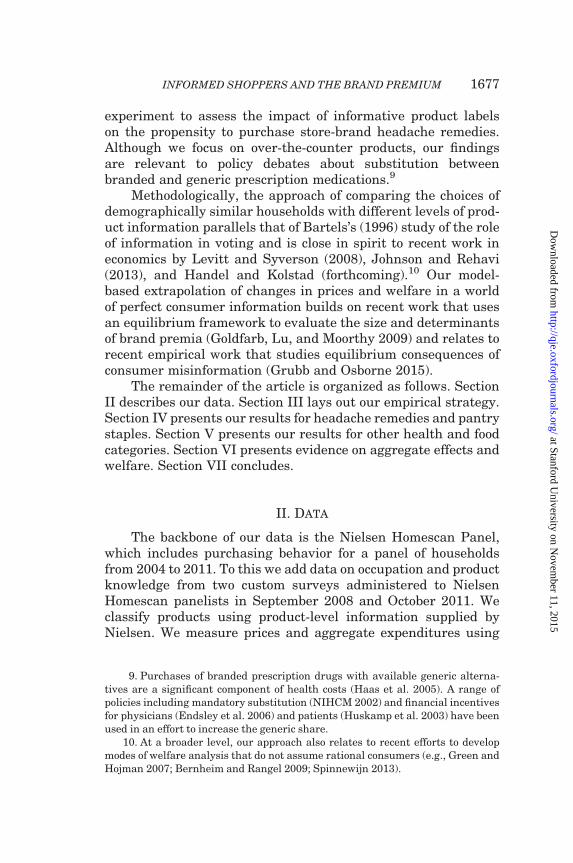
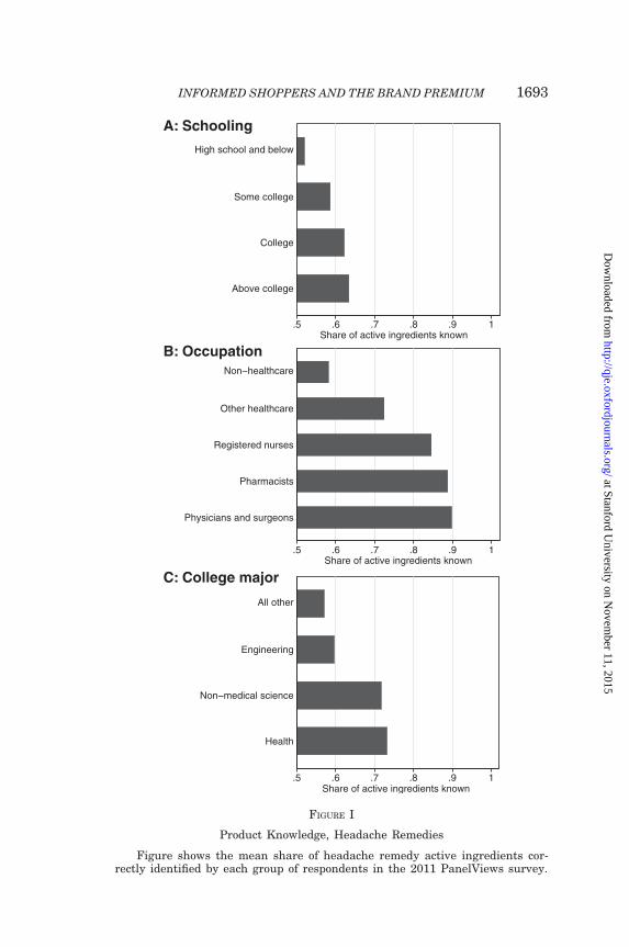
We begin the descriptive portion of our empirical analysiswith a detailed case study of headache remedies. For these prod-ucts, we measure information directly through a survey of asubset of Nielsen panelists in which we ask the panelists toname the active ingredient in various national-brand headacheremedies. This direct measure of information is highly correlatedwith our indirect proxy measures. The average respondent an-swers 59 percent of our active ingredient questions correctly. Forthe college-educated, this fraction rises to 62 percent. For thosewhose major was science or health, it is 73 percent. For registerednurses it is 85 percent, for pharmacists it is 89 percent, and forphysicians and surgeons it is 90 percent. Occupational specialtyis important enough to outweigh large differences in general

4. We address confounds related to workplace purchases (e.g., pharmacistsreceiving free samples or discounts that affect their purchasing behavior) by study-ing experts who are no longer employed at their specialty, and by studying the effectof college major.



ovember 11, 2015


ownloaded from


human capital. For example, registered nurses are far better in-formed about headache remedies than are lawyers, despitehaving completed less schooling and earning less in the labormarket on average.

We find that more informed households are consistentlymore likely to buy store-brand headache remedies. The averagehousehold devotes 74 percent of headache remedy purchases tostore brands. Controlling for household income, other demo-graphics, and interacted fixed effects for the market, chain, andquarter in which the purchase is made, a household whose pri-mary shopper correctly identifies all active ingredients is 19 per-centage points more likely to purchase a store brand than ashopper who identifies none. A household whose primary shopperbelieves that store brands are ‘‘just as safe’’ as national brands is21 percentage points more likely to purchase a store brand than ashopper who does not believe that statement.

A similar pattern emerges when we proxy for informationwith the schooling and occupation of the primary shopper.Having a college-educated primary shopper predicts an increaseof 4 percentage points, having a primary shopper with a healthcare occupation other than pharmacist or physician predicts anincrease of 8 percentage points, and having a primary shopperwho is a pharmacist or physician predicts an increase of 15 per-centage points, with pharmacists buying store brands 91 percentof the time. Primary shoppers with science majors buy more storebrands than those with other college degrees, and the effect ofoccupation is sizable among consumers not currently employed.

We find evidence that education and occupation capture var-iation similar to our more direct measures of information. Whenwe restrict attention to households whose primary shopper cor-rectly identifies all active ingredients and believes that storebrands are just as safe as national brands, the estimated effectof college education and occupation become economically smalland statistically insignificant.

In a second case study of pantry staples (salt, sugar, andbaking soda), we find that chefs devote 77 percent of their pur-chases to store brands, compared with 60 percent for the averageconsumer. The effect of being a chef is large and highly significantafter including our detailed vector of controls for income, demo-graphics, and the choice environment. Food preparers who arenot chefs are also significantly more likely to buy store brandsthan others who are demographically similar.



ovember 11, 2015


ownloaded from


We find that the effects of consumer information are largelydomain-specific. Neither knowledge of headache remedy activeingredients nor working in a health care occupation predictsstore-brand purchases in pantry staple categories. Similarly,working in a food preparer occupation other than chef does notpredict store-brand headache remedy purchases. We do find thatchefs buy more store-brand headache remedies, suggesting thatsome of their knowledge may be transferred across domains.

We extend the approach from our two case studies to the fullset of products in which there is a comparable store-brand alter-native to national brands and sufficient purchase volume to per-form a reliable analysis. Among 50 health-related categories, theeffects of knowledge of headache remedy active ingredients,working in a health care occupation other than pharmacist orphysician, and working as a pharmacist or physician are positivefor 43, 43, and 34 categories, respectively. A substantial numberof these positive coefficients—including a large share of those forover-the-counter medications—are both economically and statis-tically significant. On average across these categories, working asa pharmacist or physician reduces the probability of buying thenational brand by roughly a fourth. Results are less consistent forthe 241 food and drink categories that we study, with the effect ofbeing a chef positive for 148 categories and negative for 93.Several of the positive coefficients are economically and statisti-cally significant—including a number of pantry staples and otherproducts, such as baking mixes and dried fruit—but a large ma-jority are not individually distinguishable from zero. The averageeffect of working as a chef is to reduce the probability of buying anational brand by 2 percent. For health products, we find somesuggestive evidence that the effect of information on the propen-sity to buy the store brand is greater in categories with higheradvertising intensity and in categories with more agreementamong experts regarding the equivalence of store and nationalbrands.

Taken together, our estimates suggest that misinformationexplains a sizable portion of the brand premium in many healthcategories, as well as in certain food categories (such as pantrystaples) with little physical variation across brands. At the sametime, our results suggest a smaller role for information in the manycategories—including the majority of foods and beverages—inwhich even experts are willing to pay a premium to buy nationalbrands.



ovember 11, 2015


ownloaded from


To sharpen these conclusions, in the final section of the arti-cle we add structure to our stylized model of choice to allow us tomake quantitative statements about the effect of consumer infor-mation on welfare and pricing. We impose a set of assumptions onthe pricing conduct of retailers and manufacturers and makefunctional form assumptions about the distribution of consumerpreferences over brands and retailers. We choose the parametersof the distribution of preference heterogeneity to match themarket shares and price-cost margins of store and nationalbrand goods. We choose a parameter that governs the gap in per-ceived brand value between informed and uninformed shoppersto match our descriptive estimates of the effect of information onthe propensity to buy the store brand.

The estimated model implies that consumer informationgreatly affects the distribution of surplus in health categories.Making all consumers as informed as a pharmacist or physician,while holding prices constant at current levels, would reduce thevariable profits of the national headache remedy brands by half,equivalent to 19 percent of total expenditure. The profits of storebrands would increase by 5 percent of expenditure, and consumersurplus would increase by 4 percent of expenditure. If prices wereto adjust to reflect the change in consumer demand, the consumersurplus gains would be even greater. In health categories otherthan headache remedies, the effects are smaller, though still eco-nomically significant. In food and drink categories, by contrast,information effects are quantitatively small, with effects on prof-its and consumer surplus of a few percent in pantry staples andless than 1 percent in other food and drink products. Althoughthese conclusions are contingent on the functional form and otherassumptions embedded in the model, together with the coefficientestimates they paint a consistent picture of the relative impor-tance of information in different product categories.

We stress three caveats to our welfare conclusions. First, weconsider the effect of consumer information only on consumerchoice and product pricing. In the longer run, if consumerswere to become better informed, firms would adjust their adver-tising expenditures and product offerings, leading to additionalwelfare effects. Second, our model assumes that information perse does not affect the utility a consumer receives from a product.If, for example, believing that national-brand aspirin worksbetter actually makes national-brand aspirin more effective atreducing headaches, then informing consumers could actually



ovember 11, 2015


ownloaded from


make them worse off.5 Third, although we refer to the welfareeffects we calculate as effects of information, in fact they incor-porate all of the ways experts make decisions differently fromnonexperts. A pharmacist differs from a nonpharmacist notonly in knowing more facts about medications but also in knowingwhich facts are relevant to a given situation and knowing whatprocess to use to make good decisions about medication. Our anal-ysis is silent on which of these differences is the most importantin driving shopping behavior.

The primary substantive contribution of this study is to usenovel data and methods to quantify the importance of informationin consumer choice in an important real-world market.6 We addto existing survey and experimental evidence7 by exploitingmultiple sources of variation in consumer information, includingoccupational expertise.8 Our work complements concurrentresearch by Carrera and Villas-Boas (2013), who use a field

5. This is a limitation of any revealed-preference evidence on the effect of in-formation, but it is especially salient here as drugs are known to have brand-relatedplacebo effects (Branthwaite and Cooper 1981; Kamenica, Naclerio, and Malani2013).

6. A sizable literature examines the demographic and attitudinal correlates ofpurchasing store-brand consumer packaged goods (e.g., Dick, Jain, and Richardson1995; Richardson, Jain, and Dick 1996; Burton et al. 1998; Sethuraman and Cole1999; Kumar and Steenkamp 2007; Berges et al. 2009; Steenkamp, van Heerde, andGeyskens 2010) and generic prescription drugs (e.g., Shrank et al. 2009). A litera-ture on blind taste tests finds that consumers cannot distinguish among nationalbrands (Husband and Godfrey 1934; Allison and Uhl 1964) or between national-brand and store-brand goods (Pronko and Bowles 1949), though there are excep-tions (Mason and Batch 2009). Wills and Mueller (1989) and Caves and Greene(1996) use aggregate data to estimate the role of advertising and quality in brandpremia. Sethuraman and Cole (1999) analyze the drivers of willingness to pay fornational brands using hypothetical choices reported on a survey.

7. Existing evidence indicates that perceptions of similarity between national-and store-brand painkillers are correlated with stated purchase intentions (Cox,Coney, and Ruppe 1983; Sullivan, Birdwell, and Kucukarslan 1994). Cox, Coney,and Ruppe (1983) find that informing consumers of active ingredient similaritydoes not have a discernible effect on purchase selections.

8. We are not aware of other research on the brand preferences of health careprofessionals. An existing literature examines the health behaviors of doctors(Glanz et al. 1982), including their propensities to use certain categories of medi-cations like sleeping pills (Domenighetti et al. 1991). Most studies of the relation-ship between occupation and store-brand purchases code occupation at a high levelof aggregation (white collar, blue collar, etc.) without reference to specific expertise(see Szymanski and Busch 1987 for a review). An exception is Darden and Howell(1987), who study the effect of retail work experience on elements of ‘‘shoppingorientation,’’ such as attitudes toward store clerks.



ovember 11, 2015


ownloaded from


experiment to assess the impact of informative product labelson the propensity to purchase store-brand headache remedies.Although we focus on over-the-counter products, our findingsare relevant to policy debates about substitution betweenbranded and generic prescription medications.9

Methodologically, the approach of comparing the choices ofdemographically similar households with different levels of prod-uct information parallels that of Bartels’s (1996) study of the roleof information in voting and is close in spirit to recent work ineconomics by Levitt and Syverson (2008), Johnson and Rehavi(2013), and Handel and Kolstad (forthcoming).10 Our model-based extrapolation of changes in prices and welfare in a worldof perfect consumer information builds on recent work that usesan equilibrium framework to evaluate the size and determinantsof brand premia (Goldfarb, Lu, and Moorthy 2009) and relates torecent empirical work that studies equilibrium consequences ofconsumer misinformation (Grubb and Osborne 2015).

The remainder of the article is organized as follows. SectionII describes our data. Section III lays out our empirical strategy.Section IV presents our results for headache remedies and pantrystaples. Section V presents our results for other health and foodcategories. Section VI presents evidence on aggregate effects andwelfare. Section VII concludes.

II. Data

The backbone of our data is the Nielsen Homescan Panel,which includes purchasing behavior for a panel of householdsfrom 2004 to 2011. To this we add data on occupation and productknowledge from two custom surveys administered to NielsenHomescan panelists in September 2008 and October 2011. Weclassify products using product-level information supplied byNielsen. We measure prices and aggregate expenditures using

9. Purchases of branded prescription drugs with available generic alterna-tives are a significant component of health costs (Haas et al. 2005). A range ofpolicies including mandatory substitution (NIHCM 2002) and financial incentivesfor physicians (Endsley et al. 2006) and patients (Huskamp et al. 2003) have beenused in an effort to increase the generic share.

10. At a broader level, our approach also relates to recent efforts to developmodes of welfare analysis that do not assume rational consumers (e.g., Green andHojman 2007; Bernheim and Rangel 2009; Spinnewijn 2013).



ovember 11, 2015


ownloaded from


store-level data from 2008, also supplied by Nielsen. Finally, wemeasure wholesale prices using data from National PromotionReports’ PRICE-TRAK database. We discuss each data set inturn.

II.A. The Nielsen Homescan Panel

We obtained data from the Nielsen Homescan Panel througha partnership between the Nielsen Company and the James M.Kilts Center for Marketing at the University of Chicago BoothSchool of Business.11 The data include purchases made on morethan 77 million shopping trips by 125,114 households from 2004to 2011. Panelist households are given optical scanners and areasked to scan the barcodes of all consumer packaged goods theypurchase, regardless of outlet or store format.12

For each purchase, we observe the date, the universal prod-uct classification (UPC) code, the transaction price, an identifierfor the store chain in which the purchase was made, and the sizeof the item, which we convert to equivalent units specific to agiven product category (e.g., pill counts for headache remediesor pounds for salt). We compute the share of purchases going tostore brand or national brand products as the share weighted byequivalent units unless otherwise noted.

Nielsen supplies household demographic characteristics in-cluding the education of the household head, a categorical mea-sure of household income, number of adults, race, age, householdcomposition, home ownership, and the geographic market ofresidence.13

Nielsen recruits panelists through a mixture of direct mailand Internet advertising. Nielsen calibrates its recruitment effortto improve the representativeness of the sample according to arange of prespecified demographic characteristics. Householdsare asked to complete multiple brief surveys prior to inclusion

11. Information on access to the data from the partnership between the NielsenCompany and the James M. Kilts Center for Marketing at the University of ChicagoBooth School of Business is available at http://research.chicagobooth.edu/nielsen/.

12. The data include purchases from supermarkets, convenience stores, massmerchandisers, club stores, drug stores, and other retail channels for consumerpackaged goods.

13. A household’s geographic market is its Nielsen-defined Scantrack market.A Scantrack market can be a metropolitan area (e.g., Chicago), a combination ofnearby cities (e.g., Hartford–New Haven), or a part of a state (e.g., west Texas).There are 76 Scantrack markets in the United States.



ovember 11, 2015


ownloaded from

http://research.chicagobooth.edu/nielsen/


in the panel and are told in advance about the process of record-ing purchase information. Nielsen offers panelists regular prizedrawings, sweepstakes, and a system of ‘‘gift points.’’ See KiltsCenter for Marketing (2013) and Muth, Siegel, and Zhen (2007)for more detail on the process of recruiting and retainingpanelists.

A variety of studies have considered the representativenessof the Homescan panel.14 Aguiar and Hurst (2007) find thatHomescan panelists in Denver, CO, are similar to a comparablesample of the Panel Study of Income Dynamics. Harding,Leibtag, and Lovenheim (2012) find that the demographic char-acteristics of cigarette smokers in Homescan are similar to thosein data sets such as the Behavioral Risk Factor SurveillanceSystem or the National Health and Nutrition ExaminationSurvey.15 Lusk and Brooks (2011) find that relative to arandom digit dial sample, Homescan panelists are older, moreeducated, and more likely to be white, and that even after con-trolling for demographics, Homescan panelists are more price-sensitive in a hypothetical choice experiment.16 Consistent withthese findings, we show in the Online Appendix that Homescanpanelists purchase more store-brand products than others whoshop in the same store.

In light of the selection of the Homescan panel, there are tworeasonable ways to interpret our estimates. First, we may thinkof the estimates as internally valid for the sample of Homescanpanelists or the population that they represent. Second, we maythink of the estimates as valid for the entire population under thestrong assumption that the effect of information is homogeneous.

14. See also Zhen et al. (2009) for a comparison of expenditure data between theConsumer Expenditure Survey and the Homescan panel. Einav, Leibtag, and Nevo(2010) find that Homescan panelists are more accurate in recording quantities thanin recording prices. Accordingly, we draw on the store-level data described below formuch of the pricing information that we use in our analysis.

15. See Broda and Weinstein (2010), Handbury and Weinstein (2015), andKaplan and Menzio (forthcoming) for other recent economic applications ofHomescan data.

16. Nielsen provides projection factors to aggregate their panelists into a rep-resentative population. These projection factors are designed to match the samplefrequencies of nine demographic characteristics to the corresponding populationfrequencies. Muth, Siegel, and Zhen (2007) provide more detail on the constructionof the projection factors. As the projection factors are not designed for the subpop-ulations we study, we do not use them in our main analysis. In Appendix Table A.1we show our core results in specifications that weight by the projection factors.



ovember 11, 2015


ownloaded from

http://qje.oxfordjournals.org/lookup/suppl/doi:10.1093/qje/qjv024/-/DC1


If homogeneity fails, then our approach could understate or over-state the effect of information on brand choice, depending onwhether the effect of information on brand choice is greater orsmaller for those who do not participate in Homescan.

II.B. PanelViews Surveys

We conducted two surveys of Homescan panelists as part ofNielsen’s monthly PanelViews survey. The first survey was sentelectronically to 75,221 households in September 2008 with therequest that each adult in the household complete the surveyseparately. In total, 80,077 individuals in 48,951 households re-sponded to the survey for a household response rate of 65.1percent. The second survey was sent electronically to 90,393households in October 2011 with the request that each adult inthe household complete the survey separately. In total, 80,205individuals in 56,258 households responded to the survey for ahousehold response rate of 62.2 percent. We show in the OnlineAppendix that the administration of the survey is not associatedwith any changes in the likelihood of purchasing the store brand.The Online Appendix also compares the demographics of respon-dents to nonrespondents. Notably, we find that relative to nonre-sponding households, households that responded to the surveytend to be smaller, higher-income, more educated, and morelikely to be white.

Both surveys asked for the respondent’s current or mostrecent occupation, classified according to the 2002 Bureau ofLabor Statistics (BLS) codes (BLS 2002).17 We match these todata on the median earnings of full-time full-year workers ineach occupation in 1999 from the U.S. Census (2000). We groupoccupations into categories (health care, food preparer) using acombination of BLS-provided hierarchies and subjective judgment.The Online Appendix lists the occupations in these groupings.

The first survey included a set of additional questions relat-ing to household migration patterns. These questions were usedin the analysis of Bronnenberg, Dube, and Gentzkow (2012). Weignore them in the present analysis.

The second survey, designed for this study, included a seriesof questions about households’ knowledge and attitudes toward

17. In the small number of cases where an individual provided conflicting re-sponses to the occupation question across the two surveys, we use the value from thesecond survey.



ovember 11, 2015


ownloaded from






various products. In particular, for each of five national brands ofheadache remedy (Advil, Aleve, Bayer, Excedrin, Tylenol), weasked each respondent who indicated familiarity with a nationalbrand to identify its active ingredient from a list of six possiblechoices, or state ‘‘don’t know / not sure.’’18 For each respondent wecalculate the number of correct responses, treating ‘‘don’t know’’as incorrect. We also asked respondents whether they agreed ordisagreed with a series of statements, including ‘‘Store-brandproducts for headache remedies / pain relievers are just as safeas the brand name products,’’ with responses on a 1 (agree) to 7(disagree) scale. For each respondent, we construct an indicatorequal to 1 if the respondent chose the strongest possible agree-ment and 0 otherwise.

The second survey also asked respondents about their collegemajor using codes from the National Center for EducationStatistics (U.S. Department of Education 2012). We define twogroups of majors for analysis: health majors, which includes allmajors with the word ‘‘health’’ in their description,19 and non–health science majors, which includes all majors in the physicaland biological sciences.

Both surveys asked respondents to indicate whether they aretheir household’s ‘‘primary shopper’’ and whether they are the‘‘head of the household.’’ For each household we identify a singleprimary shopper whose characteristics we use in the analysis,following the criteria used in Bronnenberg, Dube, and Gentzkow(2012).20 In Appendix Table A.1 and the Online Appendix, weshow that our findings go largely unchanged when we incorporatedata on the characteristics of secondary shoppers into ouranalysis.

18. The correct active ingredients are ibuprofen (Advil), naproxen (Aleve), as-pirin (Bayer), aspirin-acetaminophen-caffeine (Excedrin), and acetaminophen(Tylenol). In each case, the six possible answers were the five correct active ingre-dients plus the analgesic hydrocodone.

19. Examples include ‘‘Health: medicine,’’ ‘‘Health: nursing,’’ and ‘‘Health:dentistry.’’

20. We start with all individuals within a household who respond to the survey.We then apply the following criteria in order, stopping at the point when only asingle individual is left: (i) keep only self-reported primary shopper(s) if at least oneexists; (ii) keep only household head(s) if at least one exists; (iii) keep only the femalehousehold head if both a female and a male head exist; (iv) keep the oldest individ-ual; (v)drop responses that appear tobe duplicate responses by thesame individual;(vi) select one respondent randomly.



ovember 11, 2015


ownloaded from



Throughout the article, we restrict attention to households inwhich at least one member answered the occupation question inone or both of our PanelViews surveys. The Online Appendix re-ports the number of households whose primary shopper works ineach health care and food preparer occupation.

II.C. Product Classification

Nielsen provides a set of attribute variables for each UPCcode purchased by a Homescan panelist. Some of these, such assize, are available for all categories. Others are category-specific.For example the data include a variable that encodes the activeingredient for each headache remedy in the data. We harmonizethe codes for essentially identical descriptors (e.g., ‘‘ACET’’ and‘‘ACETAMINOPHEN’’ both become ‘‘ACETAMINOPHEN’’).

We use these descriptors to aggregate UPCs into products. Aproduct is a group of UPCs that are identical on all nonsize at-tributes provided by Nielsen. For instance, in the case of head-ache remedies, a product is a combination of an active ingredient(e.g., aspirin, naproxen), form (e.g., tablet, gelcap), formula (e.g.,regular strength, extra strength), and brand (e.g., Bayer, Aleve,store brand). We classify products as store brands using Nielsen-provided codes, supplemented with manual corrections.

To compare store brands and national brands we aggregateproducts into comparable product groups, which are sets of prod-ucts that are identical on all product attributes except for brandand item size.21 We use the abbreviated term comparable to standin for comparable product group throughout the article.

We restrict attention to comparables in which we observe atleast 500 average annual purchases in Homescan, with at leastsome purchases going to both store-brand and national-brandproducts.22 We eliminate categories in which the available attrib-ute descriptors do not provide sufficient information to identifycomparable products.23 We also eliminate categories in which theaverage retail price per equivalent unit for national-brand

21. In Appendix Table A.1 we show the robustness of our main results to con-ditioning on item size.

22. We further eliminate comparable product groups in which fewer than 50retail chains ever sell a store brand according to the retail scanner data we discussin Section II.D.

23. These are: deli products, fresh produce, nutritional supplements, miscella-neous vitamins, and antisleep products.



ovember 11, 2015


ownloaded from



products is lower than store-brand products.24 This leaves uswith a universe of 420 comparables.

We analyze headache remedies and pantry staples in detail.We chose these two case studies because they have both sufficientpurchase volume and a sufficient number of expert households(health care workers and food preparers) to permit reliable anal-ysis and because our prior was that the scope for horizontaldifferentiation between national and store brands in these cate-gories would be especially small. Our universe of headache rem-edies consists of the comparables classified by Nielsen as adult,nonmigraine, daytime headache remedies. Our universe ofpantry staples consists of the comparables classified by Nielsenas table salt, sugar, or baking soda.

We restrict our sample to transactions such that at least onecomparable national-brand purchase and at least one comparablestore-brand purchase are observed in the Homescan data in thesame retail chain and quarter as the given transaction. This re-striction limits the likelihood that a national-brand product ispurchased because no store-brand alternative is available (orvice versa).

Although we compute summary statistics for the universe of420 comparables, we conduct regression analysis using only thosecomparables with at least 5,000 sample purchases. We do this toensure sufficient data to estimate models with a rich set of con-trols. With this restriction, there are 332 comparables availablefor regression analysis, including 6 headache remedies, 44 otherhealth-related products, 6 pantry staples, 235 other food anddrink products, and 41 remaining products. The OnlineAppendix lists all comparables that we use in our regressionanalysis.

II.D. Retail Scanner Data

To estimate prices and aggregate expenditure, we use 2008store-level scanner data from the Nielsen Retail MeasurementServices (RMS) files, which we obtained through a partnershipbetween Nielsen and Chicago Booth’s Kilts Center. These datacontain store-level revenue and volume by UPC and week forapproximately 38,000 stores in over 100 retail chains. We useour product classification to aggregate UPCs into products.

24. Retail prices are from retail scanner data we discuss in Section II.D. Weexclude 34 comparables based on this condition.



ovember 11, 2015


ownloaded from




For each comparable, we compute average price per equiva-lent unit for national and store brands, respectively, as the ratioof total expenditure to total equivalent units across all grocery,drug, and mass merchandise stores across all weeks in 2008. Wealso estimate total U.S. expenditure on national and store brandsrespectively by multiplying the number of equivalent units pur-chased in the Homescan data by (i) the ratio of total equivalentunits for the comparable in RMS and Homescan, (ii) the averageprice per equivalent unit, and (iii) the ratio of 2008 U.S. food,drug, and mass merchandise sales to total 2008 expenditure mea-sured in RMS.25

The sum of estimated total U.S. expenditure across thecomparables in our sample is $196 billion. If all observed equiv-alent units were purchased at the average price per equivalentunit of store brands, this sum would fall by $44 billion or 22percent.

II.E. Wholesale Price Data

We estimate retail margins by brand using data fromNational Promotion Reports’ PRICE-TRAK product, obtainedthrough Chicago Booth’s Kilts Center. These data contain whole-sale price changes and deal offers by UPC in 48 markets from2006 until 2011, along with associated product attributes suchas item and pack sizes. The data are sourced from one majorwholesaler in each market, which is representative due to theprovisions of the Robinson-Patman (Anti-Price Discrimination)Act.

We compute the average wholesale price of each product asthe unweighted average post-deal price across markets. We com-pute retail margins by matching wholesale prices with retailprices by UPC, item size, and year. We then compute themedian retail margin of national-brand and store-brand productswithin each comparable.26

25. The Annual Retail Trade Survey of the U.S. Census Bureau reports 2008annual sales in grocery stores, pharmacies and drug stores, and warehouse clubsand superstores of $512 billion, $211 billion, and $352 billion, respectively, totaling$1,075 billion (U.S. Census 2013).

26. We compute the median rather than the mean retail margin to avoid theinfluence of outlier observations that arise due to mismatch in item size or otherattributes.



ovember 11, 2015


ownloaded from


III. Model of Choice by Uninformed and Informed

Households

In this section we lay out a stylized model of choice by unin-formed and informed households. The model clarifies the assump-tions necessary to identify the effect of information on householdchoice and welfare.

III.A. Choice Model and Interpretation

Let there be a set of households indexed by i. Each householdmust choose between a national brand and a store brand of someproduct. At the store where household i shops, the national brandcosts �pi > 0 dollars more than the store brand.

Household i believes that the national brand delivers�vi � 0 more money-metric utility than the store brand, but thetrue difference is � ~vi � 0, which may be greater or lesser than�vi. The household buys the national brand if and only if�vi � �pi. We refer to the counterfactual in which the householdbuys the national brand if and only if � ~vi � �pi as informedchoice.

If �vi;� ~vi � �pi or �pi > �vi;� ~vi, then the household’s de-cision is identical under informed choice, so its welfare does notchange. If �vi � �pi > � ~vi, then under informed choice thehousehold switches from the national brand to the store brandand gains �pi �� ~vi. If � ~vi � �pi > �vi, then under informedchoice the household switches from the store brand to the na-tional brand and gains � ~vi ��pi.

The model does not specify why there is a gap between trueand perceived brand utility. However it is general enough to beconsistent with several intuitive reasons for such a gap:

(i) Perceptions of quality. Let �qi be the perceived qualitydifference between the two products and let � ~qi be thetrue difference in quality (say, clinical efficacy for a med-ication). Let mi be the household’s marginal utility ofmoney in units of quality. Then we can write �vi ¼

�qi

mi

and � ~vi ¼� ~qi

mi.

(ii) Perceptions of failure risk. The product may succeed, de-livering value v, or it may fail, delivering value v. Thesevalues are the same for the national and store brands, butthe risk of failure is different. A household perceives thatthe national brand’s risk of failure is lower by �ri, but in



ovember 11, 2015


ownloaded from


fact it is lower by �~ri. Then �vi ¼ �ri v � vÞ�

and � ~vi ¼

� ~ri v � vÞ�

.(iii) Attention to irrelevant factors. The national and store

brand differ by amounts �x1 and �x2 in each of two di-mensions (say, taste and packaging). Utility is a weightedaverage of the two dimensions. Household i attachesweight !i to the second dimension but the correct weightis 0. Then �vi ¼ 1� !ið Þ�x1 þ !i�x2 and � ~vi ¼ �x1.

Different microfoundations may be appropriate for differentproduct categories. For example, we might expect that percep-tions of failure risk are especially important for medications,whereas attention to factors like packaging is especially impor-tant for food and drinks.

Note that although our framework accommodates many rea-sons for a departure between true and perceived brand utility, itcannot accommodate cases in which information affects utilitydirectly. Suppose, for example, that the true utility informed con-sumers receive from the national brand and the store brand is thesame. Denote this � ~vinformed

i ¼ 0. Uninformed consumers receivethe same true utility from the store brand, but they receive anadditional placebo benefit from the national brand, so� ~vuninformed

i > �pi > 0. For both types, perceived and true utilityare equal. In this case, providing information to a consumer iwould cause her to lose the value of the placebo effect, and shewould suffer a welfare loss of � ~vuninformed

i ��pi instead of reapinga welfare gain of �pi.

III.B. Identifying the Welfare Gains from Informed Choice

We now consider how to recover the effect of informed choiceon the aggregate welfare of households.

Begin with the special case in which � ~vi ¼ 0 for all i. Thiswould be an appropriate assumption if we knew that national andstore brands were identical in all respects except for the branditself, and if we were prepared to assume away any psychic ben-efit of brands. In this case any household buying the nationalbrand would switch to the store brand under informed choice,gaining welfare �pi. We can compute the aggregate gain inhousehold welfare from informed choice by aggregating theprice premia paid by all households who buy the national brand.

Identification is more difficult in the more general case inwhich � ~vi is not known. Because choices are based on perceived



ovember 11, 2015


ownloaded from


utility �vi, we cannot use price variation to recover true utility� ~vi. Our approach in this article is to parameterize the relation-ship between � ~vi and �vi by assuming that more informed house-holds act according to � ~vi and less informed households actaccording to �vi.

Let �i 2 0; 1½ � be an index of household i’s information.Suppose that for all i, � ~vi ¼ � ~v and �vi ¼ �i� ~v þ 1� �ið Þ�v,where � ~v � 0 and �v � 0 are constants representing perceivedutility from the national brand for perfectly informed and per-fectly uninformed households, respectively. Suppose furtherthat all households shop in the same store, so that for all i, �pi

¼ �p for some constant �p > 0.We observe �i and an indicator yi for whether household i

chooses the store brand. There are three possible cases. If yi = 1or yi = 0 for all possible �i then �p > � ~v;�v or � ~v;�v � �p,respectively, so households do not gain from informed choice.If yi = 0 if and only if �i is below a threshold value, then �v ��p > � ~v and households buying the national brand would gain�p�� ~v from informed choice. If yi = 0 if and only if �i is above athreshold value, then � ~v � �p > �v and households buying thestore brand would gain � ~v ��p from informed choice.

From the sign of the cross-sectional relationship between yi

and �i, it is therefore possible to learn whether households as awhole are buying too much of the national brand, too much of thestore brand, or the right brand. This argument motivates ourdescriptive analysis of the relationship between household infor-mation and the propensity to buy the store brand in Sections IVand V.

Notice that the cross-sectional relationship between yi and �i

does not tell us how much households would gain from informedchoice. To recover that quantity, suppose that we observe choicesby a large number of households in which �i ¼ 1 and that we canvary the prices paid �p. Then we can learn � ~v by finding theprice gap at which informed households switch brands. Once weknow � ~v, we can compute the aggregate welfare gain from in-formed choice at current prices by aggregating the welfare gainsacross all households that buy a different brand from the onechosen by informed households. This argument motivates thestructural analysis in Section VI, in which we use a combinationof functional form and conduct assumptions to recover the neces-sary magnitudes.



ovember 11, 2015


ownloaded from


III.C. Estimation and Implementation

Here we flesh out the practical implications of the precedingdiscussion for our descriptive analysis of the effect of informationon brand choice. We defer details of our structural exercise untilSection VI.

To execute the cross-sectional test that we described, we needto ensure three conditions.

First, we need to observe variation in household information�i. We form a vector Ki of proxies for �i, including knowledge ofactive ingredients, completed schooling, college major, and occu-pation.27 These measures are proxies in the sense that we do notknow how the units of Ki map to �i. We cannot say, for example,that completing college closes the gap between true and perceivedpreferences by some given number of percentage points, as wecould if we measured �i directly. These measures are also proxiesin the sense that the correlation of an element of Ki with choice yi

reflects both a direct causal effect (e.g., knowing that Tylenol’sactive ingredient is acetaminophen directly affects choice) and anindirect effect of information correlated with Ki (e.g., consumerswho know Tylenol’s active ingredient also tend to be well in-formed about other characteristics of headache remedies).

Second, we need to compare more to less informed house-holds while holding constant prices �pi and any other contextualdrivers of choice (e.g., in-store displays or shelf position). We dothis by assuming that all such drivers are a function of observablestore and time characteristics Zi. In our preferred specifications,Zi will include interacted indicators for market, chain, and calen-dar quarter. In Appendix Table A.1, we show that our resultssurvive even richer controls for the timing and location ofpurchases.

Third, we need to compare more and less informed house-holds with identical true preferences � ~vi . This considerationmeans we need to exclude cases in which the national and storebrand differ on horizontal attributes (e.g., cherry versus orange

27. Past purchase experience may also serve as a proxy for a household’s knowl-edge of the category. As past purchases are endogenous both to preferences and tothe choice environment, we do not include this proxy in our main analysis. InAppendix Table A.1 we show that our core findings are unchanged if we estimatespecifications that control for average annual purchase volume. In these specifica-tions, higher purchase volume is consistently associated with a statistically signif-icant increase in the propensity to buy store brand.



ovember 11, 2015


ownloaded from


flavor) over which households may have different preference or-derings. We therefore focus on brand choice within comparableproduct groups that are homogeneous on measured attributes.We show empirically that preferences for measured attributes(e.g., tablet versus caplet) do not correlate with our informationproxies Ki, which supports our assumption that preferences forunmeasured horizontal attributes are not correlated with Ki.

This consideration also means we need to hold constanthouseholds’ willingness to pay for quality. Income is the mostobvious source of heterogeneity in willingness-to-pay for quality.We control for income in our analysis and find that doing so oftenstrengthens our results. We also show that a relationship be-tween information and choice is present even among occupationalgroups that are similar in socioeconomic status (e.g., lawyers andphysicians). We further control for a range of demographic char-acteristics (e.g., age and household composition). We expect thatany remaining preference heterogeneity will work against ourmain findings: if national brands are of higher quality and moreinformed households have a stronger preference for quality (phy-sicians have, if anything, a greater taste for high-quality medi-cine, and chefs have, if anything, a greater taste for high-qualityfood), our estimates will tend to understate the effect of informa-tion on choice.

To describe the relationships among choice yi, information Ki,household characteristics Xi, and choice environment Zi, we esti-mate linear probability models of the following form:

Pr yi ¼ 1jKi;Xi;Zið Þ ¼ �þ Ki�þ Xi� þ Zi�;ð1Þ

where �, �, �, and � are vectors of parameters.28 Although fornotational ease we have written the model at the level of thehousehold, a given household can make multiple purchases. Wetherefore estimate the model at the level of the purchase occa-sion, reporting standard errors that allow for correlation at thelevel of the household, and weighting transactions by purchasevolume. Appendix Table A.1 shows that our main conclusionsare unaffected if we estimate binary logit models instead oflinear probability models.

28. When we pool data across multiple comparables, we will allow the intercept� to differ by comparable.



ovember 11, 2015


ownloaded from


IV. Case Studies

IV.A. Headache Remedies

We begin our analysis with a case study of adult, nonmi-graine, daytime headache remedies. The first rows of Table Ishow summary statistics for the six comparables in this category.These products span four active ingredients, each associated witha familiar national brand: aspirin (Bayer), acetaminophen(Tylenol), ibuprofen (Advil), and naproxen (Aleve). We estimatetotal annual expenditure on these comparables to be 2:88 billiondollars. Store-brand purchases account for 74 percent of pills and53 percent of expenditures.29

On average, the per pill price of a store brand is 40 percent ofthe price of a comparable national brand. For aspirin, a matureproduct that has been off patent since 1917, the per pill price ofstore brands is 22 percent of the national-brand price. These pricedifferences are not due to differences in where these products aresold or to volume discounts: among cases in our panel in which weobserve at least one national-brand and one store-brand purchasefor the same active ingredient and package size in the samemarket, chain, and week, the per pill price paid for store brandsis on average 26 percent of the price of an equivalent nationalbrand. The median gap is 31 percent, and the national brand ischeaper in only 5 percent of cases.

Store-brand alternatives for national-brand headache reme-dies are widely available. Using our store-level data, we estimatethat 82 percent of national-brand headache remedy purchasevolume is purchased when a store brand with the same activeingredient and form and at least as many pills is sold in thesame store and quarter at a lower price.30 In our PanelViewssurvey data, only 3.6 percent of households report that no store-brand alternative was available at their last purchase.

29. Among households with multiple headache remedy purchases, 31 percentbought only store brands and 16 percent bought only national brands. The remain-ing 52 percent bought both store brands and national brands.

30. The analogous estimates at the store-month and store-week level are 77percent and 62 percent, respectively. These statistics can underestimate the avail-ability of store-brand alternatives because a store brand can be available but notpurchased in a given time period (Handbury and Weinstein 2015). These statisticscan also overstate availability because a product can be purchased but not availablethroughout the entire time period, for example due to stockouts (Matsa 2011).



ovember 11, 2015


ownloaded from


TABLE I

SUMMARY STATISTICS

Totalexpenditure($bn/year)

Store-brandshare

(volume)

Store-brandshare

($)

Price ratio(store brand/

nationalbrand)

Headache remediesAcetaminophen gelcaps 0.39 0.51 0.38 0.58Ibuprofen gelcaps 0.50 0.29 0.22 0.69Acetaminophen tablets 0.44 0.81 0.60 0.36Aspirin tablets 0.24 0.75 0.40 0.22Ibuprofen tablets 0.94 0.81 0.61 0.36Naproxen sodium tablets 0.37 0.57 0.44 0.61

Total (6) 2.88 0.74 0.53 0.40

Other health products, all (82) 10.87 0.58 0.47 0.54Other health products,

regression sample (44)8.94 0.57 0.46 0.55

Pantry staplesBaking soda 0.14 0.33 0.27 0.75Salt (iodized) 0.07 0.53 0.47 0.76Salt (plain) 0.04 0.47 0.40 0.75Sugar (brown) 0.17 0.70 0.65 0.81Sugar (granulated) 1.27 0.60 0.59 0.92Sugar (powdered) 0.13 0.72 0.70 0.88

Total (6) 1.81 0.60 0.57 0.92

Other food and drinkproducts, all (256)

134.90 0.39 0.33 0.71

Other food and drink products,regression sample (235)

122.61 0.43 0.37 0.70

Remaining products, all (70) 45.05 0.26 0.20 0.58Remaining products,

regression sample (41)31.81 0.34 0.26 0.68

Notes. Total expenditure is 2008 annual expenditure in all grocery, drug, and mass merchandisestores in the United States, estimated as described in Section II.D. Store-brand share (volume) is theshare of equivalent quantity units (pills for headache remedies, pounds for pantry staples) in each com-parable devoted to store brands in our 2004–2011 sample of the Nielsen Homescan Panel. Store-brandshare ($) is the share of expenditure devoted to store brands in our 2004–2011 sample of the NielsenHomescan Panel. Price ratio is the average price per equivalent quantity unit observed in the 2008Nielsen RMS data for store brands divided by the analogous average price for national brands. Rowsfor ‘‘headache remedies’’ and ‘‘pantry staples’’ each correspond to a single comparable product group. Rowsfor ‘‘other health products,’’ ‘‘other food and drink products,’’ and ‘‘remaining products’’ aggregate overmultiple comparable product groups, with the number of such groups shown in parentheses. Rows for ‘‘all’’refer to the universe of all comparables as defined in Section II.C. Rows for ‘‘regression sample’’ refer tothe subset of comparables analyzed in Section V. In the second through fourth columns, these aggregatesaverage over comparable product groups weighting by expenditure, except for headache remedies, wherewe weight by number of pills.



ovember 11, 2015


ownloaded from


In Figure I we look at the relationship between knowledgeof active ingredients and our indirect knowledge proxies—completed schooling, occupation, and college major. The relation-ships are as expected. Panel A shows that shoppers with a collegeeducation correctly identify the active ingredient in 62 percent ofcases, as against 52 percent for those with a high school degree orless. Panel B shows that nurses correctly identify the active in-gredient in 85 percent of cases, pharmacists in 89 percent, andphysicians and surgeons in 90 percent. Panel C shows that shop-pers whose college major is health- or science-related are moreinformed than other shoppers. In the Online Appendix, we con-firm these relationships in a regression framework, showing thatthey remain strong even after controlling for a rich set of house-hold characteristics, including income.

Having validated our proxies, we turn to our main questionof interest: the impact of information on the share of purchasesthat go to store brands. Figure II shows that greater knowledge ofactive ingredients predicts more purchases of store brands. Thosewho can name no active ingredients buy just over 60 percent storebrands. Those who can name all five active ingredients buy nearly85 percent store brands. Though these differences are large, theycould be due to reverse causality: those interested in savingmoney buy store brands and also take the time to read ingredientlabels. By contrast, while demographic characteristics like com-pleted schooling may be correlated with unobserved product pref-erences, such characteristics are most likely not determined byhouseholds’ preferences for store-brand versus national-brandproducts. We therefore turn next to examining variation in infor-mation induced by completed schooling, occupation, and collegemajor.

Figure III shows the relationship between store-brand shareand completed schooling. With no controls, we see that those witheducation beyond high school buy more store brands than thosewith a high school degree or less, but that there is no clear differ-ence between those with some college, a college degree, or morethan a college degree. The main confound here is income, whichis strongly negatively correlated with store-brand purchases.31

This is consistent with the ‘‘perceptions of quality’’ example in

31. The Online Appendix presents a plot of a household’s store-brand share ofpurchases against annual household income and confirms a strong negativerelationship.



ovember 11, 2015


ownloaded from




.5 .6 .7 .8 .9 1Share of active ingredients known

Physicians and surgeons

Pharmacists

Registered nurses

Other healthcare

Non−healthcare


Above college

College

Some college

High school and below


Health

Non−medical science

Engineering

All other

A: Schooling

B: Occupation

C: College major

FIGURE I

Product Knowledge, Headache Remedies

Figure shows the mean share of headache remedy active ingredients cor-rectly identified by each group of respondents in the 2011 PanelViews survey.



ovember 11, 2015


ownloaded from


Section III, in which households differ in both the marginal utilityof money and in the perceived quality gain from the nationalbrand. After controlling for income, we find a monotonic posi-tive relationship between completed schooling and store-brandshare.

Figure IV shows the relationship between store-brand shareand occupation. Here we see a negative relationship betweenstore-brand share and median occupational income among non–health care occupations. Households whose primary shopper is ahealth care professional buy far more store brands than others ofsimilar income. Pharmacists, physicians, and nurses buy morestore brands than lawyers, who have high levels of schoolingbut different occupational expertise.

Pharmacists, who stand out in the survey data in Figure I asamong the most informed about active ingredients, also stand outfor having the largest store-brand share among large health careoccupations. Only 8.5 percent of volume bought by pharmacistsare national-brand headache remedies, an amount small enough

.6.6

5.7

.75

.8.8

5S

tore

−br

and

shar

e of

pur

chas

es

Number of active ingredients known0 1 2 3 4 5

FIGURE II

Store-Brand Purchases and Knowledge, Headache Remedies

Horizontal axis shows the number of headache remedy active ingredientscorrectly identified in the 2011 PanelViews survey. The bars show the store-brand share of headache remedies for households in each category, weighted byequivalent volume (number of pills). Sample is restricted to panelists who an-swered all five active ingredient questions.



ovember 11, 2015


ownloaded from


to be explained by the occasional stockouts of store brands, andthe fact that some purchases are made by the nonpharmacistmember of a pharmacist’s household.32

.68

.7.7

2.7

4.7

6S

tore

−br

and

shar

e of

pur

chas

es

High schooland below

Some college College Above college

No controls Income controls

FIGURE III

Store-Brand Purchases and Education, Headache Remedies

Bars labeled ‘‘no controls’’ show the store-brand share of headache remedypurchases for households in each education category, weighted by equivalentvolume (number of pills). Bars labeled ‘‘income controls’’ show the predictedstore-brand share in each education category from a regression on indicatorsfor education categories and 19 household income categories, with the predictedvalues computed at the means of the covariates.

32. The fact that 8.5 percent of purchases by households whose primary shopperis a pharmacist are to national-brand goods suggests at first that 8.5 percent of thetime a pharmacist is willing to pay a significant price premium to buy a nationalbrand. There are three main reasons to interpret the finding differently. First, theprimary shopper need not be the only shopper in the household. In the smallnumber of cases (12 households, 37 transactions) in which a household with botha primary shopper and a secondary shopper who are pharmacists buy a headacheremedy, only 1.6 percent of purchases are to national brands. In the case of single-person households in which the only person is a pharmacist (22 households, 109transactions), only 5 percent of purchases are to national brands. Second, althoughwe have focused on transactions in retailers who stock both national brands andstore brands, some stockouts may nevertheless occur. Matsa (2011) estimates thestockout rate for over-the-counter drugs to be 2.8 percent. In the face of a stockout ofthe store brand, pharmacists who are unable to delay their purchase may switch tobuying a national-brand good. Third, although the average price premium for na-tional brands is very large in this category, there is some price variation, and



ovember 11, 2015


ownloaded from


Table II presents the relationship between store-brand shareand knowledge of active ingredients in a regression framework.The table presents estimates of equation (1), where the informa-tion variables of interest Ki are the share of active ingredientsknown and an indicator for college education. All specificationsallow the intercept � to differ by comparable. Columns (1), (2),and (3) include market and calendar quarter indicators in the

Lawyers

Pharmacists

Physicians

Registered nurses

.3.4

.5.6

.7.8

.91

Sto

re−

bran

d sh

are

of p

urch

ases

20000 40000 60000 80000 100000 120000 140000Median income in occupation ($1999)

FIGURE IV

Store-Brand Purchases and Occupation, Headache Remedies

Figure shows store-brand share of headache remedy purchases by occupa-tion (y-axis) and median earnings for full-time full-year workers in 1999 byoccupation (x-axis), weighted by equivalent volume (number of pills). Filled(colored) circles represent health care occupations. Occupation weights aregiven by the number of households whose primary shopper has the given oc-cupation in our sample (occupations with fewer than 25 such households areexcluded from the figure). The area of each circle is proportional to the occu-pation weights, with different scale for health care and non–health care occu-pations. The line is the prediction from an OLS regression of store-brand shareof purchase volume on median earnings excluding health care occupations andweighting each occupation by the occupation weights.

pharmacists may be buying when the price difference is unusually small. In theHomescan data, we find that for purchases made by households in which the pri-mary shopper is a pharmacist, the ratio of the average store-brand price to theaverage national-brand price is 6 percent greater than for the average purchase.For purchases made by households in which the only person is a pharmacist, theprice ratio is 14 percent greater than for the average purchase.



ovember 11, 2015


ownloaded from


vector of choice environment measures Zi; columns (4) and (5) addinteracted indicators for the market, chain, and calendar quarter.Column (1) includes controls for demographics other than incomein the vector of household characteristics Xi; column (2) adds thelog of imputed household income; columns (3)–(5) include incomecategory indicators.33

Column (2) shows that a 10 percent increase in householdincome reduces the propensity to purchase the store brand by

TABLE II

KNOWLEDGE AND HEADACHE REMEDY PURCHASES

Primary shoppercharacteristics (1) (2) (3) (4) (5)

College education 0.0094 0.0206 0.0212 0.0255 0.0214(0.0072) (0.0074) (0.0075) (0.0073) (0.0068)

Share of active ingredients known 0.1792 0.1805 0.1805 0.1898 0.1463(0.0111) (0.0112) (0.0111) (0.0108) (0.0105)

Log(household income) �0.0284(0.0063)

Believe store brands are ‘‘just as safe’’ 0.2058(0.0070)

Demographic controls? X X X X XMarket and quarter

fixed effects?X X X

Income categoryfixed effects?

X X X

Market-chain-quarterfixed effects?

X X

Sample Second Second Second Second Secondsurveywave

surveywave

surveywave

surveywave

surveywave

Mean of dependentvariable

0.7392 0.7392 0.7392 0.7392 0.7392

R2 0.1331 0.1351 0.1365 0.3561 0.3934Number of households 26,530 26,530 26,530 26,530 26,530Number of purchase

occasions195,268 195,268 195,268 195,268 195,268

Notes. Dependent variable: purchase is a store brand. Unit of observation is a purchase of a headacheremedy by a household. Observations are weighted by equivalent volume (number of pills). Standarderrors in parentheses are clustered by household. Household income is a categorical measure with 19possible values. In column (2) we impute each category at its midpoint and include indicators for top-codedvalues. In columns (3)–(5) we include separate indicators for each category. Demographic controls areindicators for categories of race, age, household composition, and housing ownership. ‘‘Believe store brandsare ‘just as safe’’’ means the primary shopper chose ‘‘agree’’ (1) on a 1–7 agree/disagree scale in response tothe statement ‘‘Store-brand products for headache remedies/pain relievers are just as safe as the brandname products.’’ All models include fixed effects for the comparable product group.

33. In our main specifications, we proxy for income using the categorical house-hold income variable supplied by Nielsen. Appendix Table A.1 presents specifica-tions that additionally control for average annual grocery spending and medianoccupational income.



ovember 11, 2015


ownloaded from


0.3 percentage points. Because income and education are posi-tively correlated but have opposite effects on store-brand pur-chasing, the effect of education gets larger when incomecontrols are added. In the preferred specification, column (4), col-lege education increases the propensity to buy store brand by 2.6percentage points. The effect of knowledge of active ingredients isfairly stable across specifications; column (4) shows that goingfrom knowledge of no active ingredients to knowledge of all in-creases the store-brand share by 19 percentage points.

Column (5) of Table II augments the specification in column(4) by adding to Ki an indicator for whether the shopper reportsthat store brands are ‘‘just as safe’’ as national brands. This is aless convincing measure of information than active ingredientknowledge, as the correct answer is arguably unclear. Still, it isworth noting that it is a very strong correlate of brand choice:believing store brands are just as safe as national brands has anadditional effect of 21 percentage points over and above the effectof active ingredient knowledge. The effect of having this beliefand being able to name all active ingredients correctly is 35 per-centage points.

Table III presents regression evidence on the effect of occu-pation. The model and controls in the first three columns are thesame as in columns (1), (2), and (4) of Table II, but now the vectorKi of information proxies consists of an indicator for college edu-cation, an indicator for being a pharmacist or physician, and anindicator for being in a health care occupation other than phar-macist or physician. The estimated occupation effects remainstable as we add controls. In the preferred specification ofcolumn (3) we find that being a pharmacist or physician increasesthe propensity to buy store brands by 15 percentage points; beingin another health care occupation increases the propensity by 8percentage points.

Column (4) of Table III presents evidence on the role of col-lege major. We restrict the sample to respondents who completedcollege and who reported their college major in our survey. Wefind that nonhealth science majors are 5 percentage points morelikely to buy store brand. Column (5) of Table III presents occu-pation results for the subsample of households whose primaryshoppers are not currently employed for pay. The OnlineAppendix shows that these households’ primary shoppers areless likely to be prime working age, more likely to be women,and more likely to be living with young children, relative to



ovember 11, 2015


ownloaded from




primary shoppers who are currently employed for pay. The coef-ficients on the occupation indicators remain large in magnitudeand statistically significant in this subsample, though less pre-cisely estimated than in the full sample. Taken together, columns(4) and (5) suggest our results are unlikely to be driven by factors

TABLE III

OCCUPATION AND HEADACHE REMEDY PURCHASES

Primary shoppercharacteristics (1) (2) (3) (4) (5) (6)

College education 0.0171 0.0288 0.0351 0.0431 0.0133(0.0061) (0.0064) (0.0061) (0.0100) (0.0123)

Pharmacist or physician 0.1527 0.1683 0.1529 0.1667 0.1445 0.0304(0.0296) (0.0294) (0.0295) (0.0380) (0.0493) (0.0379)

Other health care occupation 0.0792 0.0834 0.0790 0.0624 0.0489 0.0198(0.0099) (0.0098) (0.0102) (0.0172) (0.0224) (0.0160)

Health major 0.0096(0.0165)

Non–health science major 0.0507(0.0245)

Demographic controls? X X X X X XMarket and quarter

fixed effects?X X


X X X X X


X X X X

Sample All All All Collegemajor

reported

Notcurrentlyemployed

Secondsurveywave

Primary shoppersurvey response:

Know all activeingredients

X

Store brands are‘‘just as safe’’

X


0.7424 0.7424 0.7424 0.7536 0.7390 0.8732

R2 0.1166 0.1195 0.3037 0.4401 0.4330 0.6049Number of households 39,555 39,555 39,555 14,190 13,479 4,274Number of purchase

occasions279,499 279,499 279,499 92,020 103,624 33,373

Notes. Dependent variable: purchase is a store brand. Unit of observation is a purchase of a headacheremedy by a household. Observations are weighted by equivalent volume (number of pills). Standarderrors in parentheses are clustered by household. Occupation is defined as of the primary shopper’smost recent employment spell. ‘‘Health major’’ and ‘‘non–health science major’’ refer to primary shopper’sreported college major. Demographic controls are indicators for categories of race, age, household compo-sition, and housing ownership. All models include fixed effects for the comparable product group. ‘‘Knowall active ingredients’’ means the primary shopper correctly answered all questions about headacheremedy active ingredients. ‘‘Store brands are ‘just as safe’’’ means the primary shopper chose ‘‘agree’’(1) on a 1–7 agree/disagree scale in response to the statement ‘‘Store-brand products for headache rem-edies/pain relievers are just as safe as the brand name products.’’



ovember 11, 2015


ownloaded from


specific to current employment in a health care profession, suchas the availability of employee discounts or free samples. As fur-ther evidence, in the Online Appendix we use data on occupa-tional knowledge requirements to show that the propensity tobuy the store brand is greater among shoppers whose occupationsrequire medical knowledge. This holds true even if we excludeshoppers who we have classified as having occupations inhealth care.

Column (6) of Table III presents evidence on the extent towhich our direct and indirect knowledge measures capture thesame underlying variation. We repeat the preferred specificationof column (3), this time restricting to respondents who answeredall active ingredients questions correctly, and believe that storebrands are ‘‘just as safe’’ as national brands.34 Restricting atten-tion to well-informed consumers reduces the occupation coeffi-cients by more than 70 percent and renders them statisticallyindistinguishable from zero. These findings are consistent withthe interpretation that all of our measures capture variationalong a common dimension, which we interpret as information.

As further support for our identifying assumptions,Appendix Figure A.1 shows that health care professionals andnon–health care professionals look similar in their choices overobserved product attributes, such as active ingredient and phys-ical form. The Online Appendix presents analogous plots for av-erage annual purchase volume and item size, respectively.

IV.B. Pantry Staples

We now turn to the analysis of food purchases. Here ourproxies for knowledge are indicators for whether the primaryshopper is a chef (‘‘chef or head cook’’) or other food preparer.35

We begin with a case study of pantry staples: salt, sugar, andbaking soda. We choose these products because they are uniform

34. Imposing this restriction requires us to use only the sample of householdsthat responded to the second survey wave. We show in the Online Appendix that theresults from our baseline specification are comparable in this subsample.

35. Our second survey wave asked respondents to identify the most commonadditive to table salt (iodine), the scientific name for baking soda (sodium bicarbon-ate), and the most common ingredient of granulated sugar (sucrose). The share ofthese questions answered correctly is positively correlated with working as a chefbut not with being a nonchef food preparer, and is positively correlated (but notstatistically significantly so) with the propensity to buy store-brand pantry staples.Results for these knowledge measures are presented in the Online Appendix.



ovember 11, 2015


ownloaded from






in chemical composition and purpose, and thus analogous toheadache remedies in being relatively homogeneous.

The lower portion of Table I includes summary statistics forthe six comparables we classify as pantry staples: baking soda;regular iodized and plain salt (sold in boxes); and regular granu-lated, light brown, and powdered sugar (sold in bags).Collectively, these comparables account for $1.81 billion of expen-diture. Store-brand purchases account for 60 percent of volumeand 57 percent of expenditure. On average, the ratio of store-brand to national-brand price per equivalent volume is 0.92.

Figure V shows the relationship between store-brand shareand occupation. As with headache remedies, there is a strongnegative relationship between store-brand share and median oc-cupational income. Households whose primary shopper is a foodpreparer or food service manager buy more store brands than doothers of similar occupational income. Chefs—the occupationalgroup we would have expected ex ante to be most informedabout the quality of food products—buy more than 77 percentstore brands in these categories, more than any other occupationof meaningful size.

Table IV shows the relationship with occupation in a regres-sion framework. The specifications in the five columns are thesame as in the analogous columns of Table III, with the informa-tion proxies of interest Ki now consisting of an indicator for col-lege education, an indicator for being a chef, and an indicator forbeing a food preparer but not a chef. In our preferred specificationof column (3), we estimate that being a chef increases the proba-bility of buying store brands by 12 percentage points, and work-ing in a nonchef food preparation occupation increases thisprobability by 2 percentage points. These effects are somewhatsmaller in magnitude than those we estimate when we do notinclude our preferred set of controls. In contrast to headache rem-edies, we do not find any clear effect of college education. Column(4) shows that non–health science majors and health majors arenot statistically different from other college graduates. Column(5) shows that the coefficient on being a chef goes largelyunchanged when we focus on shoppers who are not currentlyemployed. The coefficient on being a nonchef food preparer fallsand becomes statistically insignificant, but its confidence intervalincludes the magnitude of our preferred estimate. These findingssuggest that the effects we estimate are not driven by mechanicaleffects of employment in the food industry.



ovember 11, 2015


ownloaded from


IV.C. Evidence on Domain Specificity

We find that health experts purchase more store-brandhealth products and that food experts purchase more store-brand food products. A natural follow-up question is whetherexperts’ knowledge is transferable outside of their domain of ex-pertise. Perhaps pharmacists’ understanding of the equivalenceof national-brand and store-brand headache remedies leads themto also recognize the likely equivalence of national-brand andstore-brand baking soda. Or perhaps their understanding doesnot translate beyond the categories with which they are directlyfamiliar.

Table V presents evidence on domain specificity. The firsttwo columns look at the effect of health care expertise on

Food service managers

Chefs

Supervisor food workers

CooksFood preparation workers

Bartenders

Food workers, other

.3.4

.5.6

.7.8

.91

Sto

re−

bran

d sh

are

of p

urch

ases

20000 40000 60000 80000 100000 120000 140000Median income in occupation ($1999)

FIGURE V

Store-Brand Purchases and Occupation, Pantry Staples

Figure shows store-brand share of pantry staple purchases by occupation(y-axis) and median earnings for full-time full-year workers in 1999 by occupa-tion (x-axis), weighted by equivalent volume (pounds). Filled (colored) circlesrepresent food preparer occupations. Occupation weights are given by thenumber of households whose primary shopper has the given occupation inour sample (occupations with fewer than 25 such households are excludedfrom the figure). The area of each circle is proportional to the occupationweights, with different scale for food preparer and non–food-preparer occupa-tions. The line is the prediction from an OLS regression of store-brand share ofpurchase volume on median earnings excluding food preparer occupations andweighting each occupation by the occupation weights.



ovember 11, 2015


ownloaded from


pantry staple purchases. Column (1) shows that the share ofheadache remedy active ingredients known has no significanteffect on the probability of purchasing store-brand pantry staples,with a confidence interval that rules out effects greater than 1.2percentage points. Column (2) shows that pharmacists, physi-cians, and other health care professionals are also not signifi-cantly more likely to buy store-brand pantry staples. Theconfidence intervals on the pharmacist-physician and otherhealth care occupation coefficients rule out effects greater than5.2 percentage points and 2.2 percentage points, respectively. Wecan confidently reject the hypothesis that these effects are aslarge as the effects we estimate for headache remedy purchases.

TABLE IV

OCCUPATION AND PANTRY STAPLE PURCHASES

Primary shoppercharacteristics (1) (2) (3) (4) (5)

College education �0.0230 �0.0060 �0.0062 �0.0023(0.0050) (0.0052) (0.0039) (0.0063)

Chef 0.1383 0.1298 0.1175 0.2079 0.1403(0.0204) (0.0197) (0.0189) (0.0513) (0.0367)

Other food preparer 0.0438 0.0344 0.0227 0.0529 0.0112(0.0132) (0.0127) (0.0101) (0.0204) (0.0157)

Health major 0.0013(0.0101)

Non–health science major 0.0243(0.0167)

Demographiccontrols?

X X X X X

Market and quarterfixed effects?

X X


X X X X


X X X

Sample All All All College major Not currentlyreported employed


0.5987 0.5987 0.5987 0.5801 0.5931

R2 0.0885 0.0922 0.3862 0.4453 0.4613Number of households 44,502 44,502 44,502 15,948 15,286Number of purchase

occasions588,484 588,484 588,484 192,026 222,918

Notes. Dependent variable: purchase is a store brand. Unit of observation is a purchase of a pantrystaple by a household. Observations are weighted by equivalent volume (pounds). Standard errors inparentheses are clustered by household. Occupation is defined as of the primary shopper’s most recentemployment spell. ‘‘Health major’’ and ‘‘non–health science major’’ refer to primary shopper’s reportedcollege major. Demographic controls are indicators for categories of race, age, household composition, andhousing ownership. All models include fixed effects for the comparable product group.



ovember 11, 2015


ownloaded from


The evidence thus suggests that health care expertise does nottranslate to behavior outside the health domain, consistent withpast evidence on the domain specificity of expertise (Levitt, List,and Reiley 2010).

The final column of Table V looks at the effect of food prep-aration expertise on headache remedy purchases. Here, we do seesome evidence of transferability: controlling for income and otherdemographics, chefs are a statistically significant 11 percentagepoints more likely to buy store-brand headache remedies thanother consumers. There is no significant effect for food preparersother than chefs.

V. Cross-Category Comparisons

V.A. Health Products

We turn next to analyzing a broad set of health products. Werestrict attention to the 6 headache remedy comparables that

TABLE V

EVIDENCE ON DOMAIN SPECIFICITY

Primary shopper characteristics (1) (2) (3)

College education �0.0048 �0.0072 0.0430(0.0048) (0.0039) (0.0061)

Share of active ingredients known �0.0012(0.0067)

Pharmacist or physician 0.0018(0.0256)

Other health care occupation 0.0056(0.0084)

Chef 0.1095(0.0340)

Other food preparer 0.0081(0.0168)

Products PantryStaples

PantryStaples

HeadacheRemedies

Mean of dependent variable 0.5978 0.5987 0.7424R2 0.4059 0.3860 0.3017Number of households 29,561 44,502 39,555Number of purchase occasions 404,372 588,484 279,499

Notes. Dependent variable: purchase is a store brand. Unit of observation is a purchase of a pantrystaple (first two columns) or headache remedy (third column) by a household. Observations are weightedby equivalent volume (pounds or number of pills). Standard errors in parentheses are clustered by house-hold. Occupation is defined as of the primary shopper’s most recent employment spell. All specificationsinclude demographic controls, income category fixed effects, comparable product group fixed effects, andmarket-chain-quarter fixed effects as in column (3) of Tables III and IV.



ovember 11, 2015


ownloaded from


we study above, and 44 additional comparables for which we ob-serve at least 5,000 purchases by households with nonmissingvalues of our demographic controls. These include other medica-tions such as cold remedies, first aid products such as bandages,and miscellaneous products such as vitamins and contact lenssolution. Nonpainkiller health categories account for $8.94 billionof expenditure per year. Store-brand purchases account for 57percent of volume. Store-brand prices are half of national-brandprices on average.

For each comparable, we run one regression to estimate theeffect of knowing headache remedy active ingredients (using thespecification in column (4) of Table II) and one to estimatethe effect of being a pharmacist or physician (using the specifica-tion in column (3) of Table III). Figures VI and VII present coef-ficients on these information proxies along with 95 percentconfidence intervals. The confidence intervals are not adjustedfor multiple hypothesis testing. We present analogous plots forthe coefficients on college education and other health care occu-pation in the Online Appendix.

To test joint hypotheses about sets of coefficients, we esti-mate our full set of regression models on 20 bootstrap replicates.In each replicate we draw a random subset of households withreplacement. For the remainder of the article, all bootstrap infer-ence will be based on these 20 replicates.36

Figure VI shows that the coefficient on active ingredientknowledge is positive in 43 out of 50 cases. The share of coefficientestimates that are positive is thus 0.86, which has a bootstrapstandard error of 0.05, and is therefore highly statistically distin-guishable from the null hypothesis of no effect (half of coefficientspositive). Consistent with the evidence on domain specificity thatwe present above, if we estimate analogous models for nonhealthcomparables, the coefficient on active ingredient knowledge ispositive in only 168 out of 282 cases, which is much closer tothe null hypothesis and highly statistically distinguishable fromthe number for health categories. Figure VIII illustrates the con-trast visually, plotting the distribution of t-statistics separatelyfor health and nonhealth comparables.

36. We use 20 replicates instead of a larger number due to computational costs.The Online Appendix compares the standard errors on our key regression coeffi-cients from our 20 replicates to those obtained from a more intensive bootstrap with200 replicates, for a random subset of 20 comparables.



ovember 11, 2015


ownloaded from




The differences among the coefficients in Figure VI are in-structive. The coefficients tend to be larger and more significantfor medications and relatively smaller for first aid and eye careproducts, suggesting that in the latter group informed shoppersperceive true quality differences. Indeed, contact lens solutions arethe only health care product we have identified where some med-ical professionals recommend patients buy national brands due to

Naproxen sodium tabletsArthritis pain remedies

Alkalizing effervescentsAcetaminophen PM tablets

Anti−gas gelcapsLaxative tablets

Acetaminophen tabletsAntacid tablets (ranitidine max strength)

Sleeping aid tabletsIbuprofen tablets

Mineral capletsContact lens solution (sensitive eyes)

Allergy tablets (loratadine)Antacid tablets (famotidine max strength)

Antacid tablets (omeprazole)Migraine tablets

Acetaminophen gelcapsAspirin tablets (low dose)

Aspirin tabletsSleeping aid mini−caplets

Multi−vitamins (with minerals)Rectal medication (ointment)

Adult incontinence (small/med)Nasal decongestant

Diarrhea remediesIbuprofen gelcaps

Contact lens solutionHydrocortisonesSheer bandagesFabric bandages

Gauze padsLaxative caplets

Antacid tablets (ranitidine)Cotton rounds

Adult incontinenceCalcium tablets

Antacid liquid (bismuth)Eye drops & lotions

Cotton swabsLaxative salts

Iron tabletsAntiseptics (hydrogen peroxide)

Digestive aids (dairy)Plastic bandages

Cotton ballsAntiseptics (alcohol)

Adult incontinence (large)Eye care (remaining)

Flexible fabric bandagesRectal medication (suppository)

−.5 0 .5Effect on probability of store−brand purchase

Headache remedies

Other medications

Remaining health products

FIGURE VI

Active Ingredient Knowledge Coefficients

Figure plots coefficients and 95 percent confidence intervals on ‘‘share ofactive ingredients known’’ for each health-related comparable product groupfrom a regression following the specification of Table II, column (4).



ovember 11, 2015


ownloaded from


quality concerns with store brands (Secor 2002). In the OnlineAppendix, we show that the estimated effects of most informationproxies tend to be larger (though not statistically significantly so)in comparables in which Consumer Reports considers store brandsand national brands to be equivalent. We also examine whetherthe effect of information is greater in the comparables for whichthe price gap between national and store brands is greatest, andfind only a weak association. Finally, we show that the effect of

Adult incontinence (small/med)Laxative tablets

Sleeping aid mini−capletsIbuprofen gelcaps

Naproxen sodium tabletsAdult incontinence (large)Antacid tablets (ranitidine)

Arthritis pain remediesAcetaminophen PM tablets

Diarrhea remediesLaxative capletsHydrocortisonesIbuprofen tabletsFabric bandages

Acetaminophen gelcapsCalcium tablets

Allergy tablets (loratadine)Adult incontinence

Mineral capletsAcetaminophen tablets

Aspirin tabletsMulti−vitamins (with minerals)

Contact lens solution (sensitive eyes)Digestive aids (dairy)

Laxative saltsAspirin tablets (low dose)

Cotton ballsCotton swabs

Plastic bandagesAntacid tablets (ranitidine max strength)

Antacid tablets (omeprazole)Flexible fabric bandages

Sheer bandagesIron tablets

Anti−gas gelcapsSleeping aid tabletsEye drops & lotions

Cotton roundsContact lens solution

Antiseptics (hydrogen peroxide)Antiseptics (alcohol)

Gauze padsAntacid tablets (famotidine max strength)

Antacid liquid (bismuth)Rectal medication (suppository)

Migraine tabletsNasal decongestant

Eye care (remaining)Alkalizing effervescents

Rectal medication (ointment)

−2 −1 0 1Effect on probability of store−brand purchase

Headache remedies

Other medications

Remaining health products

FIGURE VII

Pharmacist/Physician Occupation Coefficients

Figure plots coefficients and 95 percent confidence intervals on ‘‘pharmacistor physician’’ for each health-related comparable product group from a regres-sion following the specification of Table III, column (3).



ovember 11, 2015


ownloaded from




information tends to be greater in more advertising-intensive com-parables, consistent with the idea that perceptions of product qual-ity by the uninformed may be driven by advertising on the part ofnational-brand manufacturers.

Figure VII presents estimates of the effect of being a pharma-cist or physician; estimates of the effect of being in another healthcare occupation are presented in the Online Appendix. We seebroadly similar patterns to the coefficients on active ingredientknowledge, though with somewhat less precision. The effect ofbeing a pharmacist or physician is positive in share 0.68 of cases(bootstrap standard error = 0.05), and the effect of being in anotherhealth care occupation is positive in share 0.86 of cases (bootstrapstandard error = 0.04). In the Online Appendix we present plotsanalogous to Figure VIII for the coefficients on the pharmacist/physician indicator and the other health care occupation indicator.

It is important to stress that Figure VI shows the relationshipbetween store-brand purchase and knowledge of headache remedyactive ingredients; we do not have direct measures of knowledge

0.1

.2.3

.4D

ensi

ty

−5 0 5 10 15t−statistic on effect of knowledge of active ingredients

Non−health categories Health categoriesStandard normal

FIGURE VIII

Active Ingredient Knowledge Coefficients, Health versus Nonhealth Products

Figure plots the distribution of t-statistics on ‘‘share of active ingredientsknown’’ for all health-related and non–health-related comparable productsgroups from a regression following the specification of Table II, column (4).Distribution is estimated using an Epanechnikov kernel with optimal band-width. The standard normal density is plotted with dashed lines.



ovember 11, 2015


ownloaded from




for non–headache remedy comparables. We might therefore expectthis knowledge proxy to be most strongly related to store-brandpurchases in headache remedies and similar categories, even if thetrue effects of information are no greater in such categories. Ourcross-category analysis of occupational effects in Figure VII andthe Online Appendix is useful in part because the effects of occu-pation are not subject to this type of bias.

V.B. Food and Drink Products

Next we consider the remaining food and drink comparablesin our data. We restrict attention to the 6 pantry staples that westudy above, plus 235 additional comparables for which we ob-serve at least 5,000 purchases by households with nonmissingvalues of our demographic controls. These make up a broadcross-section of supermarket products, from milk and eggs, tocarbonated beverages, to ready-to-eat cereal. Excluding pantrystaples, these categories account for $123 billion of expenditure.Store-brand purchases account for 43 percent of volume. Onaverage, the price per equivalent volume for store brands is 70percent of that for national brands.

For each comparable, we run a separate regression to estimatethe effect of working as a chef or other food preparer on store-brandpurchases (using the specification in column (3) of Table IV).Figure IX summarizes the estimated coefficients and 95 percentconfidence intervals. Rather than try to present all coefficients in asingle figure, we aggregate comparables other than pantry staplesinto what Nielsen calls ‘‘product groups,’’ weighting the individualcomparables by precision and computing the aggregate confidenceinterval as if the individual coefficients are statistically indepen-dent. Thus, for example, the comparables for cola, diet cola, lemon-lime soda, and so forth are combined into the Nielsen productgroup ‘‘carbonated beverages.’’

The estimated effects of knowledge on store-brand purchasesin these categories are weaker than what we saw for health prod-ucts. The coefficients on working as a chef are positive for 148comparables and negative for 93. The share of coefficient esti-mates that are positive is thus 0.61, with a bootstrap standarderror of 0.04. The coefficients that are individually statisticallysignificant are generally small in magnitude. The pantry staplescategories stand out as having among the most positive and sig-nificant coefficients: granulated sugar has the third largest



ovember 11, 2015


ownloaded from



Baking mixesDried fruit

Sugar (granulated)Sugar (brown)

Dairy spreads & dipsSugar (powdered)

SoupJams & jellies

Gelatins & syrupCottage cheese, etc.

Prepared foodBaking supplies

CheeseFrozen vegetables

Pickles, olives & relishBaking soda

Dough productsSalad dressings & mayo

Canned vegetablesTable syrup & molasses

Oil & shorteningBread & baked goods

Canned seafoodFrozen fruit toppings

Dried veggies & grainsCandy

Salt (plain)Canned fruit

TeaSalt (iodized)

MilkEggs

Frozen breakfast foodsJuice drinks

Frozen juice drinksCondiments & sauces

Breakfast foodsCookiesSnacks

Frozen pizza & snacksSpices & seasonings

Butter & margarineFrozen baked goods

Ice creamYogurt

Carbonated beveragesPowdered milk

CerealNuts

Prepared food (dry)

−.5 0 .5Effect on probability of store−brand purchase

Pantry staplesOther food

FIGURE IX

Chef Coefficients

Figure plots coefficients and 95 percent confidence intervals on ‘‘chef’’ foreach food and drink category. Coefficients are estimated separately for eachcomparable in a regression following the specification of Table IV, column (3).Coefficients for pantry staples are plotted individually by comparable. We ag-gregate coefficients for all other comparables to the Nielsen product group level,reporting the precision-weighted mean of the estimated coefficients and con-structing the confidence intervals based on the harmonic mean of the estimatedvariances.



ovember 11, 2015


ownloaded from


coefficient in the figure, and three of the top six coefficients arepantry staples. In the Online Appendix we present plots analo-gous to Figure IX for working in other food preparation occupa-tions and for having a college education.

VI. Aggregate Effects of Consumer Information

In this section we add structure to the stylized model inSection III. We estimate the model using a combination of thecoefficients from the preceding analysis and additional data mo-ments. We then compute the effect of consumer information onthe distribution of consumer and producer surplus and on pricesand market shares.

The purpose of this analysis is twofold. First, we wish to ag-gregate the coefficients estimated in Section V to learn how ex-penditures, market shares, and profits would change in the drugstore and the grocery store if all households behaved like expertshoppers. This aggregation does not rely on details of the model: itamounts to an expenditure-weighted aggregation of the coeffi-cients from our linear probability models (e.g., those presentedin Figure VII), along with information on retail and wholesaleprices.

Second, we wish to predict how consumer welfare and firmpricing would change in a world of informed shoppers. Our pre-dictions are contingent on a set of strong parametric, symmetry,and conduct assumptions. These assumptions allow us to solvethe model in closed form for a large set of product categories andshow transparently how the various empirical moments deter-mine our estimates. Because the resulting model is highly styl-ized, our welfare and pricing results should be taken more assuggestive illustrations of the economic forces at work than asrealistic empirical predictions.

VI.A. Model

For each comparable, consider a market with R retailers in-dexed by r and households indexed by i. Each retailer sells a storebrand with price p 0; rð Þ and a national brand with price p 1; rð Þ.Each household must make a single purchase from the choice set0; 1f g � 1; :::;Rf g. Both the store brand and the national brand are

manufactured at constant marginal cost c.



ovember 11, 2015


ownloaded from



Each retailer sets the price of, and captures all profits from,its own store brand. A single manufacturer captures all profitsfrom the sale of the national brand and sets the price of this brandat each retailer. The assumption that the manufacturer sets thefinal retail price means that our model does not exhibit double-marginalization effects. We view this as an approximation to asetting in which the manufacturer has a rich set of instruments(wholesale prices, slotting fees, promotional allowances, resaleprice maintenance, etc.) with which to influence both the finalprice and the distribution of profits between the manufacturerand the retailer.37 We treat advertising and other marketingcosts incurred by the manufacturer as a sunk cost in the senseof Shaked and Sutton (1987) and Sutton (1989), and we assumethese costs are chosen at a prior stage that we do not model.

The market consists of a large number of uninformed house-holds—which we define as consumers who are not pharmacists orphysicians for health products and consumers who are not chefsfor food products—as well as a small number of informed house-holds. We assume the latter are few enough that firms ignorethem in making pricing decisions, and we do not include themin our welfare calculations.

Each household maximizes utility uiðb; rÞ given by

uiðb; rÞ ¼ vi bð Þ � p b; rð Þ � �i rð Þ;ð2Þ

where b 2 0; 1f g is an indicator for purchasing the nationalbrand, vi bð Þ is an idiosyncratic perceived brand preference,and �i rð Þ is an idiosyncratic travel cost distributed standardtype I extreme value up to a scale parameter. Each householdhas a true brand preference ~vi bð Þ.

We specify brand preferences as follows. We normalizevi 0ð Þ ¼ ~vi 0ð Þ ¼ 0. For each household, we let ~vi 1ð Þ ¼ l�i where lis a parameter and �i is a preference shock distributed i.i.d. logis-tic across households. For uninformed households, vi 1ð Þ ¼ �i; forinformed households, vi 1ð Þ ¼ ~vi 1ð Þ.

The parameter l� 0 indicates the similarity between trueand perceived brand preference for uninformed households.When l= 1, perceived and true brand preference agree; whenl= 0, national and store brand are truly identical but are per-ceived to be different.

37. See the discussion of vertical control in O’Brien and Shaffer (1992) andShaffer (1991).



ovember 11, 2015


ownloaded from


Throughout our analysis, we define consumer welfare withrespect to true brand preference. That is, we define the consumersurplus of a household that buys brand b at retailer r as~vi bð Þ � p b; rð Þ � �i rð Þ. We define total consumer surplus as thesum of consumer surplus across all households, and we definetotal surplus as the sum of total consumer surplus and the totalvariable profits of the manufacturer and retailers.

The game proceeds in three stages. First, the manufacturerand retailers simultaneously announce all prices p b; rð Þ. Second,each household learns its travel cost �i rð Þ and chooses which re-tailer r to visit. Third, each household learns its perceived brandpreference vi bð Þ and chooses which brand b to purchase. We re-strict our attention to a symmetric equilibrium in whichp 0; rð Þ ¼ p 0ð Þ, and hence p 1; rð Þ ¼ p 1ð Þ, for each retailer r.

VI.B. Estimation

Estimation is in closed form. Here we outline the key steps;an Appendix provides additional details.

We match p 0ð Þ and p 1ð Þ to the average store-brand and na-tional-brand prices, respectively, and we choose c to match themedian retail margin of store brands. We choose the scale of�i rð Þ to match the retailer’s markup on the store brand: greaterdispersion in �i rð Þ implies less competition among retailers andhence greater retail margins. Similarly, we choose the scale of �i

to match the manufacturer’s markup on the national brand. Givenscale parameters, we can then choose the location of �i to matchthe overall market share of the national brand: a high marketshare for the national brand implies a high mean value of �i.

Having pinned down the preferences of the uninformed, wechoose l to match the difference in store-brand purchase proba-bility between informed and uninformed consumers shown inFigures VII and IX. When informed households purchase morestore brand than uninformed households, l< 1. When informedhousehold purchase more national brands than uninformedhouseholds, l> 1.

The Online Appendix presents point estimates for all param-eters for all comparables, with bootstrapped standard errors.

VI.C. Results

Tables VI and VII present summaries of our findings, aggre-gated across groups of comparables, for health and food products,



ovember 11, 2015


ownloaded from



TA

BL

EV

I

HE

AL

TH

CA

TE

GO

RIE

SP

UR

CH

AS

ES

UN

DE

RF

UL

LIN

FO

RM

AT

ION

Hea

dach

ere

med

ies

(6)

Oth

erh

ealt

hca

tegor

ies

(44)

Base

lin

e

Info

rmed

con

sum

ers

at

base

lin

ep

rice

s

Info

rmed

con

sum

ers

at

equ

ilib

riu

mp

rice

sB

ase

lin

e

Info

rmed

con

sum

ers

at

base

lin

ep

rice

s

Info

rmed

con

sum

ers

at

equ

ilib

riu

mp

rice

s

Nati

onal-

bra

nd

qu

an

tity

share

0.2

58

0.1

17

0.2

86

0.4

35

0.3

70

0.5

06

(0.0

33)

(0.0

76)

(0.0

24)

(0.0

26)

Nati

onal-

bra

nd

pri

ce(r

elati

ve

toco

st)

6.0

36

—3.7

98

3.6

39

—3.1

81

(0.9

85)

(0.3

02)

Sto

re-b

ran

dp

rice

(rel

ati

ve

toco

st)

2.0

47

—1.9

96

1.9

49

—1.8

09

(0.1

05)

(0.0

73)

Ch

an

ge

as

ash

are

ofbase

lin

eex

pen

dit

ure

Man

ufa

ctu

rer

pro

fit

�0.1

88

�0.1

41

�0.0

53

�0.0

11

(0.0

47)

(0.0

51)

(0.0

16)

(0.0

21)

Ret

ail

erp

rofi

t0.0

53

�0.0

10

0.0

19

�0.0

34

(0.0

14)

(0.0

26)

(0.0

06)

(0.0

13)

Con

sum

erex

pen

dit

ure

�0.1

35

�0.1

51

�0.0

34

�0.0

44

(0.0

34)

(0.0

64)

(0.0

10)

(0.0

30)

Con

sum

ersu

rplu

s0.0

38

0.1

50

0.0

33

0.0

37

(0.0

21)

(0.0

64)

(0.0

07)

(0.0

32)

Tot

al

surp

lus

�0.0

97

�0.0

00

�0.0

01

�0.0

07

(0.0

25)

(0.0

09)

(0.0

08)

(0.0

05)

Base

lin

eco

nsu

mer

exp

end

itu

re($

bn

/yea

r)$2.8

8$8.9

4

Not

es.

Th

etw

op

an

els

rep

ort

resu

lts

for

hea

dach

ere

med

yco

mp

ara

ble

san

dot

her

hea

lth

com

para

ble

s,re

spec

tivel

y,

wit

hth

en

um

ber

ofco

mp

ara

ble

sin

pare

nth

eses

.T

he

‘‘base

lin

e’’co

lum

nre

por

tsaver

age

pri

ces

rela

tive

toes

tim

ate

dm

an

ufa

ctu

rin

gco

sts

an

dre

pea

tssu

mm

ary

info

rmati

onfr

omT

able

I.T

otal

exp

end

itu

reare

esti

mate

d2008

tota

lsfo

rall

gro

cery

,d

rug,

an

dm

ass

mer

chan

dis

est

ores

inth

eU

nit

edS

tate

s.H

ead

ach

ere

med

yre

lati

ve

pri

ces

an

dn

ati

onal-

bra

nd

share

sare

aver

aged

over

com

para

ble

pro

du

ctgro

up

sw

eigh

tin

gby

equ

ivale

nt

un

its

sold

,w

hil

eot

her

hea

lth

cate

gor

yre

lati

ve

pri

ces

an

dn

ati

onal-

bra

nd

share

sare

aver

aged

over

com

para

ble

pro

du

ctgro

up

sw

eigh

tin

gby

exp

end

itu

re.

Th

e‘‘i

nfo

rmed

con

sum

ers

at

base

lin

ep

rice

s’’

cou

nte

rfact

ual

com

pu

tes

the

effe

ctof

all

hou

seh

old

sch

oosi

ng

acc

ord

ing

totr

ue

rath

erth

an

per

ceiv

edbra

nd

pre

fere

nce

,h

old

ing

pri

ces

con

stan

tat

base

lin

ele

vel

s.T

he

‘‘in

form

edco

nsu

mer

sat

equ

ilib

riu

mp

rice

s’’c

oun

terf

act

ual

furt

her

all

ows

pri

ces

toad

just

tore

flec

tth

ech

an

ge

inco

nsu

mer

dem

an

d.

Sta

nd

ard

erro

rsin

pare

nth

eses

are

from

20

boo

tstr

ap

rep

lica

tion

sin

wh

ich

we

dra

wh

ouse

hol

ds

at

ran

dom

wit

hre

pla

cem

ent

an

dre

com

pu

teall

esti

mate

s.T

hes

est

an

dard

erro

rsth

us

acc

oun

tfo

rco

rrel

ati

onin

sam

pli

ng

erro

racr

oss

com

para

ble

s.S

eeS

ecti

onV

Ifo

rd

etail

sof

mod

elsp

ecifi

cati

onan

des

tim

ati

on.



ovember 11, 2015


ownloaded from


TA

BL

EV

II

FO

OD

AN

DD

RIN

KP

UR

CH

AS

ES

UN

DE

RF

UL

LIN

FO

RM

AT

ION

Pan

try

stap

les

(6)

Oth

erfo

odan

dd

rin

kca

tegor

ies

(235)

Base

lin

eIn

form

edco

nsu

mer

sIn

form

edco

nsu

mer

sB

ase

lin

eIn

form

edco

nsu

mer

sIn

form

edco

nsu

mer

sat

base

lin

ep

rice

sat

equ

ilib

riu

mp

rice

sat

base

lin

ep

rice

sat

equ

ilib

riu

mp

rice

s

Nati

onal-

bra

nd

qu

an

tity

share

0.4

04

0.3

11

0.4

34

0.5

75

0.5

65

0.5

74

(0.0

23)

(0.0

08)

(0.0

09)

(0.0

06)

Nati

onal-

bra

nd

pri

ce(r

elati

ve

toco

st)

1.3

12

—1.2

50

1.9

62

—2.0

10

(0.0

13)

(0.0

39)

Sto

re-b

ran

dp

rice

(rel

ati

ve

toco

st)

1.1

46

—1.1

34

1.3

46

—1.3

43

(0.0

03)

(0.0

05)

Ch

an

ge

as

ash

are

ofbase

lin

eex

pen

dit

ure

Man

ufa

ctu

rer

pro

fit

�0.0

18

�0.0

16

�0.0

05

0.0

05

(0.0

04)

(0.0

04)

(0.0

05)

(0.0

07)

Ret

ail

erp

rofi

t0.0

08

�0.0

08

0.0

03

�0.0

01

(0.0

02)

(0.0

02)

(0.0

02)

(0.0

02)

Con

sum

erex

pen

dit

ure

�0.0

10

�0.0

24

�0.0

02

0.0

04

(0.0

02)

(0.0

06)

(0.0

03)

(0.0

08)

Con

sum

ersu

rplu

s0.0

02

0.0

26

0.0

04

�0.0

04

(0.0

01)

(0.0

06)

(0.0

01)

(0.0

10)

Tot

al

surp

lus

�0.0

08

0.0

01

0.0

02

0.0

00

(0.0

02)

(0.0

01)

(0.0

04)

(0.0

03)

Base

lin

eco

nsu

mer

exp

end

itu

re($

bn

/yea

r)$1.8

1$122.6

1

Not

es.

Th

etw

op

an

els

rep

ort

resu

lts

for

pan

try

stap

les

com

para

ble

san

dot

her

food

an

dd

rin

kco

mp

ara

ble

s,re

spec

tivel

y,

wit

hth

en

um

ber

ofco

mp

ara

ble

sin

pare

nth

eses

.T

he

‘‘base

lin

e’’co

lum

nre

por

tsaver

age

pri

ces

rela

tive

toes

tim

ate

dm

an

ufa

ctu

rin

gco

sts

an

dre

pea

tssu

mm

ary

info

rmati

onfr

omT

able

I.T

otal

exp

end

itu

reare

esti

mate

d2008

tota

lsfo

rall

gro

cery

,d

rug,

an

dm

ass

mer

chan

dis

est

ores

inth

eU

nit

edS

tate

s.R

elati

ve

pri

ces

an

dn

ati

onal-

bra

nd

share

sare

aver

aged

over

com

para

ble

pro

du

ctgro

up

sw

eigh

tin

gby

exp

end

itu

re.

Th

e‘‘i

nfo

rmed

con

sum

ers

at

base

lin

ep

rice

s’’

cou

nte

rfact

ual

com

pu

tes

the

effe

ctof

all

hou

seh

old

sch

oosi

ng

acc

ord

ing

totr

ue

rath

erth

an

per

ceiv

edbra

nd

pre

fere

nce

,h

old

ing

pri

ces

con

stan

tat

base

lin

ele

vel

s.T

he

‘‘in

form

edco

nsu

mer

sat

equ

ilib

riu

mp

rice

s’’co

un

terf

act

ual

furt

her

all

ows

pri

ces

toad

just

tore

flec

tth

ech

an

ge

inco

nsu

mer

dem

an

d.

Sta

nd

ard

erro

rsin

pare

nth

eses

are

from

20

boo

tstr

ap

rep

lica

tion

sin

wh

ich

we

dra

wh

ouse

hol

ds

at

ran

dom

wit

hre

pla

cem

ent

an

dre

com

pu

teall

esti

mate

s.T

hes

est

an

dard

erro

rsth

us

acc

oun

tfo

rco

rrel

ati

onin

sam

pli

ng

erro

racr

oss

com

para

ble

s.S

eeS

ecti

onV

Ifo

rd

etail

sof

mod

elsp

ecifi

cati

onan

des

tim

ati

on.



ovember 11, 2015


ownloaded from


respectively. For each set of products we present the change rel-ative to baseline from two counterfactuals in which householdschoose according to true rather than perceived brand preference.In the first counterfactual, prices are held constant at observedlevels; in the second, prices adjust to reflect the change in con-sumer demand. We measure changes in consumer expenditureand surplus, and changes in retailer and manufacturer profit,relative to baseline expenditure levels. Tables VI and VII useour estimated parameter values. As a benchmark, the OnlineAppendix presents analogous results in which we impose l= 0regardless of the estimated l.

The left panel of Table VI presents results for headache rem-edies. Holding prices constant at baseline levels, if all consumersbecame as informed as pharmacists or physicians, the marketshare of national-brand headache remedies would fall by half,total expenditure on headache remedies would fall by 14 percent,and consumer surplus would increase by 4 percent relative tobaseline expenditure. The national-brand manufacturer wouldlose profits equivalent to 19 percent of baseline expenditure,and retailers would gain profits equivalent to 5 percent. Notethat total surplus falls even though we evaluate consumer wel-fare with respect to true preferences. The reason is that whilemanufacturing costs are equal across brands, prices are not.Because even experts perceive some small differences amongbrands (l> 0), shifting purchases toward store brands entailssome loss of social efficiency. To illustrate this intuition, theOnline Appendix shows that the change in total surplus getssmaller as national-brand prices approach store-brand prices.

Allowing prices to adjust softens the blow for the national-brand manufacturer by allowing the manufacturer to lower therelative price of the national brand. This harms retailers but in-creases the gains to the consumer. Because prices come to betterreflect manufacturing costs, total surplus rises relative to thecase in which prices are held constant, and there is no aggregateefficiency loss relative to baseline. In addition, calculations notreported in the table show that informed households benefit frommaking all households informed, because prices fall for both na-tional-brand and store-brand goods.

The right panel of Table VI shows that for other health cat-egories we find effects that are similar directionally to those forheadache remedies, smaller in magnitude, and still economicallysignificant. Allowing for price adjustment, consumers would gain



ovember 11, 2015


ownloaded from





surplus equivalent to 4 percent of baseline expenditure in healthcategories other than headache remedies, were they to chooseaccording to their true preferences. Additional results presentedin the Online Appendix show that much of this gain would comefrom (non–headache remedy) medication categories.

Table VII examines food and drink categories. Here, thesmall price differences between national and store brands andthe relatively modest effects of information combine to implyfairly small impacts. The greatest effect is found in pantry sta-ples, where allowing for both price adjustment and greater con-sumer information would improve consumer welfare by anamount equal to 3 percent of baseline expenditure.

The calculations in Tables VI and VII imply that at currentprices, the average household would gain $7.92 a year in con-sumer surplus from being as informed as a pharmacist or physi-cian when making health-related purchases and as informed as achef when making food purchases. Put differently, if informationis costly to acquire, households would optimally choose to be asinformed as an expert if the cost of doing so were less than $7.92and would choose to remain uninformed if the cost were greaterthan $7.92. Of course, these calculations consider only the bene-fits to information in the comparables that we study; there maywell be benefits to expert information in other consumer domains(e.g., decisions about elective surgical procedures).

VII. Conclusions

Across a range of products, we find strong evidence that moreinformed shoppers buy more store brands and fewer nationalbrands. Consumer information plays a large quantitative rolein health categories, where our estimates imply that expendi-tures and market shares would change significantly if all house-holds behaved like expert shoppers. By contrast, the role ofconsumer information is smaller in food and drink categories,where our estimates suggest much smaller gaps between expertand nonexpert shopping behavior.

We do not perform any quantitative policy evaluation in thearticle. However, we think our findings and methods may be rel-evant to several active policy areas. One such area is the regula-tion of ‘‘copycat’’ products that are designed to look like otherbrands. Regulators, especially in Europe, have considered the



ovember 11, 2015


ownloaded from



possibility that store-brand products with such copycat packag-ing might ‘‘lead consumers to think that the [store-brand] productis . . . of similar quality’’ to the national brand (UK CompetitionCommission 2008).38 Our findings imply that at least in someproduct categories, consumers exhibit the opposite bias, believingthat national brands are better than store brands when in factthey are not. In those categories, copycat packaging could raiseconsumer welfare by signaling that different brands are of similarquality.

A second area of potential policy relevance is the regulation ofdeceptive advertising. The U.S. Federal Trade Commission evalu-ates claims of deceptive advertising on whether the advertising isindeed deceptive and on whether the deception is ‘‘material,’’ forexample to the consumer’s purchase decision. A common method-ology for establishing deceptiveness is a copy test, in which con-sumers are shown the advertisements in question and asked tointerpret them (see, e.g., Federal Trade Commission 1999). Acommon methodology for establishing materiality is to survey con-sumers to ask what factors influence their decisions (Richards andPreston 1992). Our article suggests comparing the behavioral re-sponse of experts and nonexperts as a possible choice-based ap-proach to quantifying the harm from a potentially deceptiveadvertising claim or campaign. If experts respond differentlythan nonexperts, that may be taken as consistent with misinfor-mation; our model suggests one way to quantify the costs of thatmisinformation to nonexpert consumers.

In considering these and other policy implications, it is worthstressing that our study is limited to examining the effects ofinformation on brand choice and prices. If consumers were tobecome more informed, markets would adjust on other marginsas well. For example, although our analysis takes as given thedecision to purchase in a given category, better information couldalso lead consumers to change which product categories they buyin, and how much they buy. Turning to the supply side, a moreinformed population of consumers might change whether andhow much firms choose to advertise their products, as well aswhich products are introduced to the market. Taking account ofthese forms of adjustment, and examining their implications forwelfare is an important priority for future work.

38. See also section 2.4.4 of the European Commission’s Unfair CommercialPractices Guidance (European Commission 2014).



ovember 11, 2015


ownloaded from


APPENDIX TABLE A.1

KNOWLEDGE AND HEADACHE REMEDY PURCHASES, ROBUSTNESS

Headache remedies

Pantrystaples

Share ofactive

ingredientscoefficient

Collegeeducationcoefficient

Pharmacist/physiciancoefficient

Chefcoefficient

(1) Baseline 0.1898 0.0351 0.1529 0.1175(0.0108) (0.0061) (0.0295) (0.0189)

(2) Control for market-chain-week 0.2038 0.0316 0.1888 0.1118(0.0142) (0.0076) (0.0379) (0.0220)

(3) Control for market-chain-store-quarter 0.2067 0.0325 0.1137 0.1101(0.0174) (0.0095) (0.0530) (0.0259)

(4) Control for market-chain-store-week 0.2305 0.0290 0.1904 0.0995(0.0294) (0.0146) (0.0849) (0.0463)

(5) Control for average annual purchase volume 0.1828 0.0371 0.1438 0.1066(0.0109) (0.0062) (0.0293) (0.0189)

(6) Control for average annual grocery spending 0.1924 0.0319 0.1534 0.1195(0.0108) (0.0061) (0.0285) (0.0191)

(7) Control for median occupational income 0.1905 0.0350 0.1528 0.1147(0.0108) (0.0063) (0.0319) (0.0189)

(8) Condition sample on item size availability 0.1786 0.0404 0.1375 0.0998(0.0122) (0.0066) (0.0384) (0.0215)

(9) Condition sample on item size availabilityand control for item size

0.1691 0.0366 0.1349 0.0974

(0.0118) (0.0064) (0.0376) (0.0204)(10) Weight observations by Nielsen 0.1879 0.0532 0.1180 0.1092

projection factor(0.0137) (0.0085) (0.0334) (0.0242)

(11) Impute characteristics of actual shopper 0.1969 0.0405 0.1578 0.1256(0.0110) (0.0068) (0.0332) (0.0224)

(12) Logit controlling for market and quarter 0.2119 0.0327 0.2240 0.1290(0.0100) (0.0062) (0.0461) (0.0210)

Notes. Dependent variable: purchase is a store brand. Each row gives (i) the coefficient on ‘‘share ofactive ingredients known’’ from a specification analogous to Table II, column (4); (ii) the coefficient on‘‘college education’’ from a specification analogous to Table III, column (3); (iii) the coefficient on ‘‘phar-macist or physician’’ from a specification analogous to Table III, column (3); and (iv) the coefficient on‘‘chef’’ from a specification analogous to Table IV, column (3). Row (1) repeats the results from our mainspecifications. Row (2) is the same as the baseline but replaces market-chain-quarter fixed effects withmarket-chain-week fixed effects. Row (3) is the same as the baseline but replaces market-chain-quarterfixed effects with market-chain-store-quarter fixed effects. Row (4) is the same as the baseline but replacesmarket-chain-quarter fixed effects with market-chain-store-week fixed effects. Row (5) is the same as thebaseline but adds a control for the average annual volume of headache remedies (columns (1)–(3)) andpantry staples (column (4)) purchased by the household. Row (6) is the same as the baseline but adds acontrol for the household’s average annual grocery spending. Row (7) is the same as the baseline but addsa control for the median income of the occupation of the primary shopper. Row (8) is the same as thebaseline but restricts attention to transactions such that at least one comparable national-brand purchaseand at least one comparable store-brand purchase are observed in the Homescan data in the same retailchain, quarter, and item size as the given transaction. Row (9) is the same as row (8) but replacescomparable product group fixed effects with comparable product group-item size fixed effects. Row (10)is the same as the baseline but weights observations by the Nielsen projection factor. Row (11) is the sameas the baseline but imputes characteristics of the actual shopper by assuming that the primary shopper isthe actual shopper when there is no secondary shopper and that the primary shopper is the actualshopper 74 percent of the time when there is a secondary shopper; see the Online Appendix for details.Row (12) is the same as the baseline but replaces the linear probability model with a logit model and themarket-chain-quarter fixed effects with market and quarter fixed effects; observations are not weightedand reported coefficients are average marginal effects.



ovember 11, 2015


ownloaded from



Appendix: Details of Model Estimation and Computation

We estimate parameters separately for each comparable pro-duct group. Let the brand preference shock �i be distributed logis-tic with location parameter and scale parameter brand.39 Defineretail so that �i rð Þ

retailis distributed standard type I extreme value.

The parameters to be estimated are ; brand; retail;R; lf g.Let S be the population market share of the store brand for

uninformed households. From the properties of the logistic dis-tribution, it is immediate that

0.2

.4.6

.81

Sha

re o

f pur

chas

es

Ibuprofengelcap

Acetaminophengelcap

Naproxentablet

Aspirintablet

Acetaminophentablet

Ibuprofentablet

Non−healthcare Healthcare

APPENDIX FIGURE A.1

Physical Attribute Choice and Occupation, Headache Remedies

Share of purchases is computed from a set of linear probability models ofthe likelihood of purchasing the given product. Bars labeled ‘‘healthcare’’ showthe predicted probability from the given model for purchases made by house-holds whose primary shopper is in a health care occupation. Bars labeled ‘‘non-healthcare’’ show the predicted probability for the same purchases under thecounterfactual in which the household’s primary shopper is not in a health careoccupation. Each linear probability model’s unit of observation is a purchaseoccasion. Observations are weighted by equivalent volume (number of pills). Allspecifications include an indicator for college completion, demographic controls,income category fixed effects, and market-chain-quarter fixed effects.Demographic controls are dummies for categories of race, age, householdcomposition, and housing ownership. Predicted probabilities set the market-chain-quarter fixed effect so that the mean predicted probability is equal tothe empirical share. See the Online Appendix for a supporting table with ad-ditional details.

39. With this parameterization, the mean of �i is and the variance is�22

brand3 .



ovember 11, 2015


ownloaded from



S ¼ logit�1 �p�

brand

� �;ð3Þ

where �p � p 1ð Þ � p 0ð Þ and logit�1 xð Þ ¼ 1þ exp �xð Þð Þ�1.

Begin with estimation of and brand. It is possible to showthat in a symmetric interior equilibrium the manufacturer’s first-order condition is

pð1Þ � c ¼1� S

dSdp 1ð Þ

;ð4Þ

where

dS

dp 1ð Þ¼

S 1� Sð Þ

brand:ð5Þ

Given p 0ð Þ; p 1ð Þ, and c, equations (3), (4), and (5) imply uniquevalues of and brand for a given S. We estimate and brand bysubstituting the sample analogue of S into the resultingexpressions.

Turn next to estimation of retail and R. These are notseparately identified but for our purposes it is sufficient toidentify ~ retail �

RR�1 retail. To do this we observe that in a sym-

metric interior equilibrium the price of the store brand must satisfy

pð0Þ � c ¼S

~ retailþ

dS

dp 1ð Þ

1

S

� ��1

:ð6Þ

Given p 0ð Þ; p 1ð Þ, c, equations (4) and (6) define a unique ~retail

as a function of S. We estimate ~ retail by substituting thesample analogue of S into the resulting expression.

The final parameter to estimate is l. Let Sl be the populationmarket share of the store brand for informed households:

Sl ¼ logit�1�pl �

brand

!:ð7Þ

It follows that:

l ¼�p

brand logit Slð Þ � logit Sð Þð Þ þ�p:ð8Þ

We estimate l by substituting sample analogues of S and Sl

into this expression.We use the linear probability models reported in Figures VII

(for health categories) and IX (for food categories) to definesample analogues of Sl and S for each comparable. For a given



ovember 11, 2015


ownloaded from


comparable, denote these sample analogues by Sl and S, respec-tively. We define an expert to be a pharmacist or physician forhealth categories and a chef for nonhealth categories. We defineSl to be the mean predicted probability of choosing store brand ifeach purchaser i were an expert with the average expert’s level ofeducation and the purchaser’s own demographics Xi and choiceenvironment Zi. We define S so that the average of Sl and S,weighted by the sample shares of experts and nonexperts, isequal to the overall share choosing store brand.

A few exceptional cases are worth noting. When, for a givencomparable, the data described in Section II.E do not include thestore-brand retail margin or imply a negative store-brand retailmargin, we impute the store-brand retail margin as the expendi-ture-weighted average store-brand retail margin across othercomparables in the same group (health/food). When, for a givencomparable, the linear probability model reported in Figure VII(for health categories) or Figure IX (for food categories) impliesthat Sl � 1, we impute l= 0. When the linear probability modelimplies that Sl � 0, or when no value of l 2 0; l�

�explains Sl, we

set l equal to an upper bound l. We use the threshold l ¼ 3 in ourestimates. Finally, when no value of ~ retail solves equation (6), weassume in computing counterfactuals that prices are fixed at p 0ð Þand p 1ð Þ. We summarize the frequency of these cases in theOnline Appendix.

To compute counterfactual prices under informed choice,we solve equations (4) and (6) numerically assuming thatdemand is governed by informed rather than uninformed prefer-ences. Exact expressions for the change in consumer welfareunder informed choice are readily derived from the assumed pre-ference structure.40

40. Fixing baseline prices, for l � 1 the gain to the average uninformed consu-mer from choosing according to informed preferences is given by:Z �p

l

�p�p� l�ið ÞdF �ið Þ;ð9Þ

where FðÞ is the CDF of the distribution of �i. This integral exists in closed

form, as does the analogue for the case of l>1.



ovember 11, 2015


ownloaded from



Tilburg School of Economics and Management,

CentER, and CEPR

University of Chicago Booth School of Business and NBER

Stanford University and NBER

Brown University and NBER

Supplementary Material

An Online Appendix for this article can be found at QJEonline (qje.oxfordjournal.org).

References

Aguiar, Mark, and Erik Hurst, ‘‘Life-Cycle Prices and Production,’’ AmericanEconomic Review, 97 (2007), 1533–1559.

Allison, Ralph I., and Kenneth P. Uhl, ‘‘Influence of Beer Brand Identification onTaste Perception,’’ Journal of Marketing Research, 1 (1964), 36–39.

Associated Press, ‘‘Contaminated with Metal, a Painkiller Is Recalled,’’ New YorkTimes, November 10, 2006, accessed March 29, 2013, available at http://www.nytimes.com/2006/11/10/health/10recall.html.

Bartels, Larry M., ‘‘Uninformed Votes: Information Effects in PresidentialElections,’’ American Journal of Political Science, 40 (1996), 194–230.

Becker, Gary S., and Kevin M. Murphy, ‘‘A Simple Theory of Advertising as aGood or Bad,’’ Quarterly Journal of Economics, 108 (1993), 941–964.

Berges, Fabian, Daniel Hassen, Sylvette Monier-Dilhan, and Helene Raynal,‘‘Consumers’ Decision Between Private Labels and National Brands in aRetailer’s Chain: A Mixed Multinomial Logit Application,’’ Gestion 2000, 3(2009), 41–57.

Bernheim, B. Douglas, and Antonio Rangel, ‘‘Beyond Revealed Preference:Choice-Theoretic Foundations for Behavioral Welfare Economics,’’Quarterly Journal of Economics, 124 (2009), 51–104.

Braithwaite, Dorothea, ‘‘The Economic Effects of Advertisement,’’ EconomicJournal, 38 (1928), 16–37.

Branthwaite, Alan, and Peter Cooper, ‘‘Analgesic Effects of Branding inTreatment of Headaches,’’ British Medical Journal, 282 (1981), 1576–1578.

Broda, Christian, and David E. Weinstein, ‘‘Product Creation and Destruction:Evidence and Price Implications,’’ American Economic Review, 100 (2010),691–723.

Bronnenberg, Bart J., Jean-Pierre Dube, and Matthew Gentzkow, ‘‘The Evolutionof Brand Preferences: Evidence from Consumer Packaged Goods,’’ AmericanEconomic Review, 102 (2012), 2472–2508.

Bureau of Labor Statistics, 2002 Census Occupation Classification, 2002, http://www.bls.gov, accessed January 4, 2010.

Burton, Scot, Donald R. Lichtenstein, Richard G. Netemeyer, and JudithA. Garretson, ‘‘A Scale for Measuring Attitude toward Private LabelProducts and an Examination of its Psychological and BehavioralCorrelates,’’ Journal of the Academy of Marketing Science, 26 (1998), 293–306.

Carrera, Mariana, and Sofia Villas-Boas, ‘‘Generic Aversion and ObservationalLearning in the Over-the-Counter Drug Market,’’ Case Western WorkingPaper, 2013.

Caves, Richard E., and David P. Greene, ‘‘Brands’ Quality Levels, Prices, andAdvertising Outlays: Empirical Evidence on Signals and InformationCosts,’’ International Journal of Industrial Organization, 14 (1996), 29–52.

Cox, Steven R., Kenneth A. Coney, and Peter F. Ruppe, ‘‘The Impact ofComparative Product Ingredient Information,’’ Journal of Public Policy &Marketing, 2 (1983), 57–69.



ovember 11, 2015


ownloaded from


http://www.nytimes.com/2006/11/10/health/10recall.html

http://www.nytimes.com/2006/11/10/health/10recall.html

http://www.bls.gov

http://www.bls.gov


Darden, William R., and Roy D. Howell, ‘‘Socialization Effects of Retail WorkExperience on Shopping Orientations,’’ Journal of the Academy ofMarketing Science, 15 (1987), 52–63.

Dick, Alan, Arun Jain, and Paul Richardson, ‘‘Correlates of Store BrandProneness: Some Empirical Observations,’’ Journal of Product & BrandManagement, 4 (1995), 15–22.

Domenighetti, Gianfranco, Michele Tomamichel, Felix Gutzwiller,Silvio Berthoud, and Antoine Casabianca, ‘‘Psychoactive Drug Use amongMedical Doctors Is Higher than in the General Population,’’ Social Science& Medicine, 33 (1991), 269–274.

Einav, Liran, Ephraim Leibtag, and Aviv Nevo, ‘‘Recording Discrepancies inNielsen Homescan Data: Are They Present and Do They Matter?,’’Quantitative Marketing and Economics, 8 (2010), 207–239.

Ellison, Glenn, and Alexander Wolitzky, ‘‘A Search Cost Model of Obfuscation,’’RAND Journal of Economics, 43 (2012), 417–441.

Endsley, Scott, Geof Baker, Bernard A. Kershner, and Kathleen Curtin, ‘‘WhatFamily Physicians Need to Know about Pay for Performance,’’ FamilyPractice Management, 13 (2006), 69–74.

European Commission, ‘‘European Commission Guidance on Unfair CommercialPractices,’’ 2014, accessed November 19, 2014, available at https://webgate.ec.europa.eu/ucp/public/index.cfm?event=public.guidance.browse&elemID=74.

Federal Trade Commission, ‘‘Final Order In the Matter of Novartis Corporation,et al., Docket 9279,’’ 1999, available at http://www.ftc.gov/os/decisions/docs/Volume127.pdf.

Gabaix, Xavier, and David Laibson, ‘‘Shrouded Attributes, Consumer Myopia, andInformation Suppression in Competitive Markets,’’ Quarterly Journal ofEconomics, 121 (2006), 505–540.

Glanz, Karen, Stanley B. Fiel, Lawrence R. Walker, and Marvin R. Levy,‘‘Preventive Health Behavior of Physicians,’’ Journal of Medical Education,57 (1982), 637–639.

Goldfarb, Avi, Qiang Lu, and Sridhar Moorthy, ‘‘Measuring Brand Value in anEquilibrium Framework,’’ Marketing Science, 28 (2009), 69–86.

Green, Jerry R., and Daniel A. Hojman, ‘‘Choice, Rationality, and WelfareMeasurement,’’ Harvard University Working Paper, 2007.

Grubb, Michael D., and Matthew Osborne, ‘‘Cellular Service Demand: BiasedBeliefs, Learning, and Bill Shock,’’ American Economic Review, 105 (2015),234–271.

Haas, Jennifer S., Kathryn A. Phillips, Eric P. Gerstenberger, and AndrewC. Seger, ‘‘Potential Savings from Substituting Generic Drugs for Brand-name Drugs: Medicare Expenditure Panel Survey, 1997–2000,’’ Annals ofInternal Medicine, 142 (2005), 891–897.

Handbury, Jessie, and David E. Weinstein, ‘‘Goods Prices and Availability inCities,’’ Review of Economic Studies, 82 (2015), 258–296.

Handel, Benjamin, and Jonathan T. Kolstad, ‘‘Health Insurance for ‘Humans’:Information Frictions, Plan Choice, and Consumer Welfare,’’ AmericanEconomic Review, forthcoming.

Harding, Matthew, Ephraim Leibtag, and Michael F. Lovenheim, ‘‘TheHeterogeneous Geographic and Socioeconomic Incidence of CigaretteTaxes: Evidence from Nielsen Homescan Data,’’ American EconomicJournal: Economic Policy, 4 (2012), 169–198.

Hortacsu, Ali, and Chad Syverson, ‘‘Product Differentiation, Search Costs, andCompetition in the Mutual Fund Industry: A Case Study of S&P 500 IndexFunds,’’ Quarterly Journal of Economics, 119 (2004), 403–456.

Husband, Richard W., and Jane Godfrey, ‘‘An Experimental Study of CigaretteIdentification,’’ Journal of Applied Psychology, 18 (1934), 220–223.

Huskamp, Haiden A., Patricia A. Deverka, Arnold M. Epstein, Robert S. Epstein,Kimberly A. McGuigan, and Richard G. Frank, ‘‘The Effect of Incentive-Based Formularies on Prescription-Drug Utilization and Spending,’’ NewEngland Journal of Medicine, 349 (2003), 2224–2232.

Johnson, Erin M., and M. Marit Rehavi, ‘‘Physicians Treating Physicians:Information and Incentives in Childbirth,’’ NBER Working Paper 19242,2013.



ovember 11, 2015


ownloaded from

https://webgate.ec.europa.eu/ucp/public/index.cfm?event=public.guidance.browse&elemID=74

https://webgate.ec.europa.eu/ucp/public/index.cfm?event=public.guidance.browse&elemID=74

http://www.ftc.gov/os/decisions/docs/Volume127.pdf

http://www.ftc.gov/os/decisions/docs/Volume127.pdf


Kamenica, Emir, Robert Naclerio, and Anup Malani, ‘‘Advertisements Impact thePhysiological Efficacy of a Branded Drug,’’ Proceedings of the NationalAcademy of Sciences, 110 (2013), 12931–12935.

Kaplan, Greg, and Guido Menzio, ‘‘The Morphology of Price Dispersion,’’International Economic Review, forthcoming.

Kilts Center for Marketing, ‘‘Nielsen Consumer Panel Dataset Manual,’’ KiltsCenter Archive of the Nielsen Company, 2013.

Kumar, Nirmalya, and Jan-Benedict E. M. Steenkamp, Private Label Strategy:How to Meet the Store Brand Challenge (Cambridge, MA: Harvard BusinessSchool Press, 2007).

Levitt, Steven D., John A. List, and David H. Reiley, ‘‘What Happens in the FieldStays in the Field: Exploring Whether Professionals Play Minimax inLaboratory Experiments,’’ Econometrica, 78 (2010), 1413–1434.

Levitt, Steven D., and Chad Syverson, ‘‘Market Distortions When Agents AreBetter Informed: The Value of Information in Real Estate Transactions,’’Review of Economics and Statistics, 90 (2008), 599–611.

Lusk, Jayson L., and Kathleen Brooks, ‘‘Who Participates in Household ScanningPanels?,’’ American Journal of Agricultural Economics, 93 (2011), 226–240.

Mason, Kevin, and Alice Batch, ‘‘What’s in a (Brand) Name?,’’ Proceedings ofAmerican Society of Business and Behavioral Sciences, 16 (2009).

Matsa, David A., ‘‘Competition and Product Quality in the SupermarketIndustry,’’ Quarterly Journal of Economics, 126 (2011), 1539–1591.

Muth, Mary K., Peter H. Siegel, and Chen Zhen, ‘‘Homescan Data Description,’’ ERAData Quality Study Design, 2007, accessed November 16, 2014, available at http://qed.econ.queensu.ca/jae/2007-v22.7/hausman-leibtag/Homescan-data.pdf.

National Institute for Health Care Management (NIHCM), A Primer: GenericDrugs, Patents, and the Pharmaceutical Marketplace (Washington, DC:National Institute for Health Care Management Foundation, 2002).

O’Brien, Daniel P., and Greg Shaffer, ‘‘Vertical Control with Bilateral Contracts,’’RAND Journal of Economics, 23 (1992), 299–308.

Piccione, Michele, and Ran Spiegler, ‘‘Price Competition under LimitedComparability,’’ Quarterly Journal of Economics, 127 (2012), 97–135.

Pronko, Nicholas H., and J. W. Bowles Jr., ‘‘Identification of Cola Beverages. III. AFinal Study,’’ Journal of Applied Psychology, 33 (1949), 605–608.

Richards, Jef I., and Ivan L. Preston, ‘‘Proving and Disproving Materiality ofDeceptive Advertising Claims,’’ Journal of Public Policy and Marketing, 11(1992), 45–56.

Richardson, Paul S., Arun K. Jain, and Alan Dick, ‘‘Household Store BrandProneness: A Framework,’’ Journal of Retailing, 72 (1996), 159–185.

Scherer, Frederic M., Industrial Market Structure and Economic Performance(Chicago: Rand McNally, 1970).

Secor, Glenda B., ‘‘Educate Patients about Inconsistency of Generic Contact LensSolutions,’’ Primary Care Optometry News, May 2002, available at http://www.healio.com/optometry/contact-lenses-eye-wear/news/print/primary-care-optometry-news/%7Ba6af06d9-ffe3-4a21-88a2-10f963172c5a%7D/edu-cate-patients-about-inconsistency-of-generic-contact-lens-solutions.

Sethuraman, Raj, and Catherine Cole, ‘‘Factors Influencing the Price Premiumsthat Consumers Pay for National Brands over Store Brands,’’ Journal ofProduct & Brand Management, 8 (1999), 340–351.

Shaffer, Greg, ‘‘Slotting Allowances and Resale Price Maintenance: A Comparisonof Facilitating Practices,’’ RAND Journal of Economics, 22 (1991), 120–135.

Shaked, Avner, and John Sutton, ‘‘Product Differentiation and IndustrialStructure,’’ Journal of Industrial Economics, 36 (1987), 131–146.

Shrank, William H., Emily R. Cox, Michael A. Fischer, Jyostna Mehta, andNiteesh K. Choudhry, ‘‘Patients’ Perceptions of Generic Medications,’’Health Affairs, 28 (2009), 546–556.

Simons, Henry, Economic Policy for a Free Society (Chicago: University of ChicagoPress, 1948).

Smith, Michael D., and Erik Brynjolfsson, ‘‘Consumer Decision-Making at anInternet Shopbot: Brand Still Matters,’’ Journal of Industrial Economics,49 (2001), 541–558.



ovember 11, 2015


ownloaded from

http://qed.econ.queensu.ca/jae/2007-v22.7/hausman-leibtag/Homescan-data.pdf

http://qed.econ.queensu.ca/jae/2007-v22.7/hausman-leibtag/Homescan-data.pdf

http://www.healio.com/optometry/contact-lenses-eye-wear/news/print/primary-care-optometry-news/%7Ba6af06d9-ffe3-4a21-88a2-10f963172c5a%7D/educate-patients-about-inconsistency-of-generic-contact-lens-solutions





Spinnewijn, Johannes, ‘‘Insurance and Perceptions: How to Screen Optimists andPessimists,’’ Economic Journal, 123 (2013), 606–633.

Steenkamp, Jan-Benedict E. M., Harold J. van Heerde, and Inge Geyskens, ‘‘WhatMakes Consumers Willing to Pay a Premium for National Brands overPrivate Labels,’’ Journal of Marketing Research, 47 (2010), 1011–1024.

Sullivan, Donald L., Stephen W. Birdwell, and Suzan N. Kucukarslan, ‘‘AnAssessment of Consumer Purchasing Behavior for Private-Label vs. Brand-Name Over-the-Counter Products in Chain Pharmacies,’’ Journal ofPharmaceutical Marketing & Management, 8 (1994), 85–108.

Sullivan, Mary W., ‘‘How Brand Names Affect the Demand for TwinAutomobiles,’’ Journal of Marketing Research, 35 (1998), 154–165.

Sutton, John, ‘‘Endogenous Sunk Costs and the Structure of AdvertisingIntensive Industries,’’ European Economic Review, 33 (1989), 335–344.

Szymanski, David M., and Paul S. Busch, ‘‘Identifying the Generics-ProneConsumer: A Meta-Analysis,’’ Journal of Marketing Research, 24 (1987),425–431.

Thomas, Katie, ‘‘An Increase in Scrutiny for Generics,’’ New York Times, October31, 2012, available at http://www.nytimes.com/2012/11/01/business/fda-in-creases-scrutiny-of-some-generic-drugs.html.

U.K. Competition Commission, ‘‘The Supply of Groceries in the UK: MarketInvestigation,’’ 2008, available at http://www.ias.org.uk/uploads/pdf/Price%20docs/538.pdf.

U.S. Census, ‘‘Earnings by Occupation and Education, 1999,’’ 2000, accessedDecember 17, 2009, available at http://www.census.gov/hhes/www/income/earnings/earnings.html.

———, ‘‘Monthly Retail Trade Report: Estimates of Monthly Retail and FoodServices Sales by Kind of Business: 2008,’’ 2013, available at http://www.census.gov/retail/.

U.S. Department of Education, Institute of Education Sciences, National Centerfor Education Statistics (NCES), ‘‘CIP User Site,’’ available at http://nces.ed.gov/ipeds/cipcode/Default.aspx?y=55.

Wills, Robert L., and Willard F. Mueller, ‘‘Brand Pricing and Advertising,’’Southern Economic Journal, 56 (1989), 383–395.

Zhen, Chen, Justin L. Taylor, Mary K. Muth, and Ephraim Leibtag,‘‘Understanding Differences in Self-Reported Expenditures betweenHousehold Scanner Data and Diary Survey Data: A Comparison ofHomescan and Consumer Expenditure Survey,’’ Review of AgriculturalEconomics, 31 (2009), 470–492.



ovember 11, 2015


ownloaded from

http://www.nytimes.com/2012/11/01/business/fda-increases-scrutiny-of-some-generic-drugs.html

http://www.nytimes.com/2012/11/01/business/fda-increases-scrutiny-of-some-generic-drugs.html

http://www.ias.org.uk/uploads/pdf/Price%20docs/538.pdf

http://www.ias.org.uk/uploads/pdf/Price%20docs/538.pdf

http://www.census.gov/hhes/www/income/earnings/earnings.html

http://www.census.gov/hhes/www/income/earnings/earnings.html

http://www.census.gov/retail/

http://www.census.gov/retail/

http://nces.ed.gov/ipeds/cipcode/Default.aspx?y=55

http://nces.ed.gov/ipeds/cipcode/Default.aspx?y=55


Documents

I. Introduction - Stanford Universityweb.stanford.edu/~gentzkow/research/generics.pdfpharmacists choosing them over store brands only 9 percent of the time, com pared to 26 percent