Propagation of Systemic Risk in Interbank Networks

Vanessa Hoffmann de Quadros,1 Juan Carlos Gonzalez-Avella,1 and Jose Roberto Iglesias1, 2

1Instituto de Fısica, Universidade Federal do Rio Grande do Sul,Caixa Postal 15051, 90501-970 Porto Alegre RS, Brazil

2Programa de Mestrado em Economia, Universidade do Vale do Rio dos Sinos,Av. Unisinos, 950, 93022-000 Sao Leopoldo RS, Brazil

(Dated: October 24, 2018)

Abstract One of the most striking characteristics of modern financial systems is its complex in-terdependence, standing out the network of bilateral exposures in interbank market, through whichinstitutions with surplus liquidity can lend to those with liquidity shortage. While the interbankmarket is responsible for efficient liquidity allocation, it also introduces the possibility for systemicrisk via financial contagion. Insolvency of one bank can propagate through the network leading toinsolvency of other banks. Moreover, empirical studies reveal that some interbank networks havefeatures of scale-free networks, which means that the distribution of connections among banks fol-lows a power law. This work explores the characteristics of financial contagion in networks whoselinks distributions approaches a power law, using a model that defines banks balance sheets frominformation of network connectivity. By varying the parameters for the creation of the network, sev-eral interbank networks are built, in which the concentrations of debts and credits are obtained fromlinks distributions during the creation networks process. Three main types of interbank network areanalyzed for their resilience to contagion: i) concentration of debts is greater than concentration ofcredits, ii) concentration of credits is greater than concentration of debts and iii) concentrations ofdebts and credits are similar. We also tested the effect of a variation in connectivity in conjunc-tion with variation in concentration of links. The results suggest that more connected networkswith high concentration of credits (featuring nodes that are large creditors of the system) presentgreater resilience to contagion when compared with the others networks analyzed. Evaluating sometopological indices of systemic risk suggested by the literature we have verified the ability of theseindices to explain the impact on the system caused by the failure of a node. There is a clear positivecorrelation between the topological indices and the magnitude of losses in the case of networks withhigh concentration of debts. This correlation is smaller for more resilient networks.

Resumo Uma das caracterısticas mais marcantes dos sistemas financeiros modernos e sua complexainterdependencia, destacando-se a rede de exposicoes bilaterais no mercado interbancario, atravesdo qual as instituicoes com liquidez excedente podem emprestar para aqueles com falta de liquidez.Enquanto o mercado interbancario e responsavel pela alocacao eficiente de liquidez, tambem introduza possibilidade de risco sistemico atraves de contagio financeiro. A insolvencia de um banco podese propagar atraves da rede, levando a insolvencia outros bancos. Alem disso, os estudos empıricosrevelam que algumas redes interbancarias tem caracterısticas de redes livres de escala, que significaque a distribuicao das conexoes entre os bancos segue uma lei de potencias. Este trabalho exploraas caracterısticas do contagio financeiro em redes cuja distribuicao de conexoes se aproxima deuma lei de potencia, utilizando um modelo que define o balance financeiro dos bancos usando asinformacoes de conectividade de rede. Variando os parametros para a criacao da rede, varias redesinterbancarias sao construıdas, em que as concentracoes de debitos e creditos sao obtidas a partir dedistribuicoes de ligacoes durante o processo de construcao das redes. Tres tipos principais de redeinterbancaria sao analisados segundo sua resiliencia ao contagio: i) concentracao de dıvidas maiorque a concentracao de creditos, ii) concentracao de creditos maior do que a concentracao de dıvidase iii) concentracoes de dıvidas e creditos semelhantes. Testamos tambem o efeito de uma variacaona conectividade em conjunto com a variacao na concentracao de links. Os resultados sugerem queredes mais conectadas e com alta concentracao de creditos (apresentando nos que sao os grandescredores do sistema) apresentam maior resiliencia ao contagio quando comparado com as outrasredes analisadas. Avaliando alguns ındices topologicos de risco sistemico sugeridos pela literaturapodemos verificar a capacidade destes ındices para explicar o impacto no sistema causado pela falhade um no. Ha uma correlacao positiva entre os ındices topologicos e a magnitude das perdas no casode redes com alta concentracao de dıvidas. Esta correlacao e menor para redes mais resistentes.

Keywords: interbank exposures, power laws, systemic risk, complex networks, financial crashes.Palavras chave: Exposicao interbancaria, leis de potencia, risco sistemico, redes complexas, crisisfinanceiras.JEL Classification: G01, G21.Classificacao ANPEC: Area 8

arX

iv:1

410.

2549

v1 [

q-fi

n.G

N]

9 O

ct 2

014

2

I. INTRODUCTION

The financial crisis started in 2007 highlighted, once again, the high degree of interdependence of financial systems.A combination of excessive borrowing, risky investments, lack of transparency and high interdependence led thefinancial system to the worst financial meltdown since the Great Depression (FCIC [1]). An increasing interest infinancial contagion, motivated by the crisis, gave rise to several works in this field in the last years, although thesubject is not new.

The interdependence of financial systems exhibits multiple channels. Financial institutions are connected throughmutual exposures created in the interbank market, through which institutions with surplus liquidity can lend to thosewith liquidity shortage. While the interbank market is responsible for efficient liquidity allocation, it also introducesthe possibility for credit risk via financial contagion. Insolvency of one bank can propagate through its links leadingto insolvency of other banks. Equally important, financial institutions are indirectly connected by holding similarassets exposures and by sharing the same mass of depositors.

With respect to the direct connections of mutual exposures, the structure of interdependence can be easily capturedby using a network representation, in which the nodes of the network represent financial institutions, while the linksrepresent exposures between nodes (Allen and Babus [2]). Mutual exposures networks are directed networks in whichin links stand for credits while out links represent debts. The link direction indicates the cash flow at the time ofdebt payment (from debtor to creditor) and also indicates the direction of impact or financial loss in case of defaultof borrowers.

Theoretical studies (Allen and Gale [3], Freixas et. al. [4]) have shown that the possibility for contagion viamutual exposures depends on the precise structure of the interbank market. Allen and Gale [3] assess the contagiongenerated from an increased demand for liquidity (liquidity shock) of a system consisting of 4 identical regions. Theydemonstrate that if the system formed by these 4 regions is a complete network, in which all nodes have connectionsto each other, then contagion effect is minimized. The authors argue that in complete networks the impact of aliquidity crisis in one region may be distributed among all others and thus attenuated. Similar results are found byFreixas et. al. [4] in a model with money-centre banks.

In recent studies, different models of complex network have been used to generate artificial interbank networks, inorder to identify if a given network is more or less prone to contagion.

Nier et al. [5] simulate contagion from the initial failure of a bank in an Erdos-Renyi random network, finding anegative nonlinear relationship between contagion and the level of capitalization of banks. The relationship betweencontagion and connectivity is also nonlinear. An increase in the number of interbank exposures initially has no effecton contagion, since the losses are absorbed by the capital of each affected node. However, as the number of connectionsis raised, contagion increases until the point where further increase in connectivity cause contagion to decline. Thenon-monotonic relationship between connectivity and contagion found by the authors reflects the action of two effects:on the one hand, the addition of new links adds new channels through which contagion can occur. On the other hand,increasing links also represent the distribution of losses among a larger number of nodes, diluting the impact of thefailure and mitigating the effects of the crisis.

Studying a specific case of power-law network, Cont and Moussa [6] find similar results as Nier et al. [5] for therelation between connectivity, level of capitalization and contagion.

Battiston et al. [7] simulate contagion on a regular network and also find a nonlinear relationship between con-nectivity and contagion, but with opposite effect: initially the increase in the number of connections decreases thenetwork contagion, while later additions make contagion to increase.

The differences in the results indicate that the possibility and extent of contagion depends considerably on thestructure of each network and specific assumptions of each model.

Empirical studies reveal that some interbank networks have features of scale-free networks: this means that thedistribution of connections among banks follows a power law, p(k) ∼ k−X (Boss et al. [8], Cont et al. [9], Soramakiet al. [10], Inaoka et al. [11]). In general terms, some of the most outstanding features reported in the literature are:

• Networks have low density of links, that is, they are far from complete;

• Asymmetrical in-degree and out-degree distribution;

• Power law distributions for in and out-degree whose exponent varies around 2 and 3.

It is also noteworthy the characteristic reported by Cont et al. [9] in the study of the Brazilian network: there isa positive association between the size of exposures (assets) and the number of debtors (in-degree) of an institution,and a positive association between the size of liabilities and the number of creditors (out-degree) of an institution.More (less) connected financial institutions have larger (smaller) exposures (links weights).

3

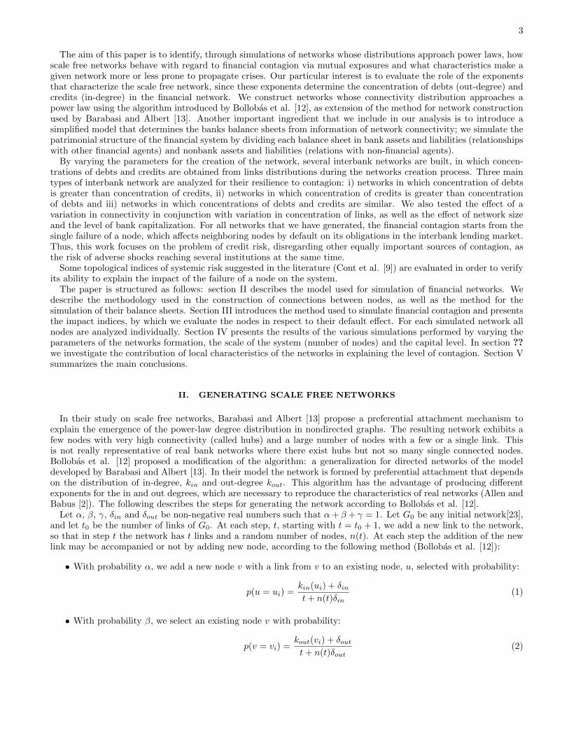
The aim of this paper is to identify, through simulations of networks whose distributions approach power laws, howscale free networks behave with regard to financial contagion via mutual exposures and what characteristics make agiven network more or less prone to propagate crises. Our particular interest is to evaluate the role of the exponentsthat characterize the scale free network, since these exponents determine the concentration of debts (out-degree) andcredits (in-degree) in the financial network. We construct networks whose connectivity distribution approaches apower law using the algorithm introduced by Bollobas et al. [12], as extension of the method for network constructionused by Barabasi and Albert [13]. Another important ingredient that we include in our analysis is to introduce asimplified model that determines the banks balance sheets from information of network connectivity; we simulate thepatrimonial structure of the financial system by dividing each balance sheet in bank assets and liabilities (relationshipswith other financial agents) and nonbank assets and liabilities (relations with non-financial agents).

By varying the parameters for the creation of the network, several interbank networks are built, in which concen-trations of debts and credits are obtained from links distributions during the networks creation process. Three maintypes of interbank network are analyzed for their resilience to contagion: i) networks in which concentration of debtsis greater than concentration of credits, ii) networks in which concentration of credits is greater than concentrationof debts and iii) networks in which concentrations of debts and credits are similar. We also tested the effect of avariation in connectivity in conjunction with variation in concentration of links, as well as the effect of network sizeand the level of bank capitalization. For all networks that we have generated, the financial contagion starts from thesingle failure of a node, which affects neighboring nodes by default on its obligations in the interbank lending market.Thus, this work focuses on the problem of credit risk, disregarding other equally important sources of contagion, asthe risk of adverse shocks reaching several institutions at the same time.

Some topological indices of systemic risk suggested in the literature (Cont et al. [9]) are evaluated in order to verifyits ability to explain the impact of the failure of a node on the system.

The paper is structured as follows: section II describes the model used for simulation of financial networks. Wedescribe the methodology used in the construction of connections between nodes, as well as the method for thesimulation of their balance sheets. Section III introduces the method used to simulate financial contagion and presentsthe impact indices, by which we evaluate the nodes in respect to their default effect. For each simulated network allnodes are analyzed individually. Section IV presents the results of the various simulations performed by varying theparameters of the networks formation, the scale of the system (number of nodes) and the capital level. In section ??we investigate the contribution of local characteristics of the networks in explaining the level of contagion. Section Vsummarizes the main conclusions.

II. GENERATING SCALE FREE NETWORKS

In their study on scale free networks, Barabasi and Albert [13] propose a preferential attachment mechanism toexplain the emergence of the power-law degree distribution in nondirected graphs. The resulting network exhibits afew nodes with very high connectivity (called hubs) and a large number of nodes with a few or a single link. Thisis not really representative of real bank networks where there exist hubs but not so many single connected nodes.Bollobas et al. [12] proposed a modification of the algorithm: a generalization for directed networks of the modeldeveloped by Barabasi and Albert [13]. In their model the network is formed by preferential attachment that dependson the distribution of in-degree, kin and out-degree kout. This algorithm has the advantage of producing differentexponents for the in and out degrees, which are necessary to reproduce the characteristics of real networks (Allen andBabus [2]). The following describes the steps for generating the network according to Bollobas et al. [12].

Let α, β, γ, δin and δout be non-negative real numbers such that α+ β + γ = 1. Let G0 be any initial network[23],and let t0 be the number of links of G0. At each step, t, starting with t = t0 + 1, we add a new link to the network,so that in step t the network has t links and a random number of nodes, n(t). At each step the addition of the newlink may be accompanied or not by adding new node, according to the following method (Bollobas et al. [12]):

• With probability α, we add a new node v with a link from v to an existing node, u, selected with probability:

p(u = ui) =kin(ui) + δint+ n(t)δin

(1)

• With probability β, we select an existing node v with probability:

p(v = vi) =kout(vi) + δoutt+ n(t)δout

(2)

4

and add a link from v to an existing node u, chosen with probability:

p(u = ui) =kin(ui) + δint+ n(t)δin

(3)

• With probability γ, we add a new node u with a link from an existing node v to u, where v is selected withprobability:

p(v = vi) =kout(vi) + δoutt+ n(t)δout

(4)

where kin(ui) is the in-degree of node ui and kout(vi) is the out-degree of node vi. Since the probability β refersto the addition of a link without any creation of a node, increasing the value of β implies increasing the averagenetwork connectivity. In turn, the parameters α and γ are related to the addition of new nodes while increasing theconnectivity of existing nodes.

As stated above, for interbank networks the in-degree of a node, kin, represents its number of debtors, so largevalues of α tends to generate nodes that concentrate many credits, i.e., the most connected nodes are large creditors.In a complementary way, large values of γ (as opposed to α) tend to generate large debtors nodes. On the other hand,the parameters δin and δout represent weights distributed among the nodes, causing everyone to have a chance ofbeing selected in the attachment process. For example, with δin > 0, even a node without any in link can be selectedto receive an in link with probability:

p(u = ui) =δin

t+ n(t)δin(5)

The similar situation occurs when we have δout > 0.In their work, Bollobas et al. [12] show that, when the number of nodes goes to infinity and the connectivity grows,

we have:

p(kin) ∼ CINk−XINin (6)

p(kout) ∼ COUT k−XOUTout (7)

where:

XIN = 1 +1 + δin(α+ γ)

α+ β(8)

XOUT = 1 +1 + δout(α+ γ)

β + γ(9)

The limit N → ∞ can obviously not be achieved, but the result is valid when the number of nodes grows and wetake the more connected ones, i.e., power laws for kin and kout will emerge in the tail of the distribution of largenetworks. Performing several simulations using different parameter values we find that, as the network grows, theconvergence to the limit values occurs from the left, i.e., from lower values than predicted by the formulas of XIN

and XOUT .We want to compare networks with different values for XIN and XOUT (featuring different concentrations of kin

and kout), while keeping other characteristics similar, such as average connectivity and total concentration of linksdistribution. We are particularly interested in networks whith values of XIN and XOUT around 2 and 3, in agreementwith estimated empirical values (for example, Boss et al. [8], Cont et al. [9], Soramaki et al. [10]). We restrict thedegrees of freedom of the model, imposing the following constraints on the parameters:

α+ γ = 0, 75 (10)

δin + δout = 4 (11)

5

For α+ γ = 0, 75, we have β = 0, 25. Since β is the probability of creating a link without addition of a new node,we can not use a value of β too small, otherwise we will have a network with very low average connectivity. On theother hand, we would like to have values of α and γ high enough for creating asymmetry between the distributionsof in-degrees and out-degrees. The values α + γ = 0, 75 and β = 0, 25 satisfy those requirements. For example, theasymmetry between the exponents estimated XIN and XOUT for networks of 1000 nodes is apparent if we use valuesα and γ in the ratio of 1:3 (or 3:1), which implies, with α + γ = 0, 75, the values α = 0.1875 and β = 0.5625 (orα = 0.5625 and β = 0.1875).

Also the differences between δin and δout cause asymmetry between the estimated exponents XIN and XOUT . Weuse δin and δout in the both ratios 1:3 and 3:1, in order to accentuate the asymmetry of the network.

In addition to the equations 10 and 11, we will cover the spaces of parameters α × γ e δout × δin by varying thefollowing radial lines:

α =δoutδin

γ → α =4− δinδin

γ (12)

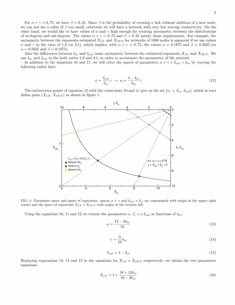
The intersection points of equation 12 with the constraints 10 and 11 give us the set (α, γ, δin, δout), which in turndefine pairs (XIN , XOUT ) as shown in figure 1.

0246810γ, δ

in

0

2

4

6

8

10

α, δout

α + γ = 0.75δout + δin = 4

2 4 6 8 10Xin

2

7Xout

Xout = (Xin+15)/(Xin-1)

Network GD0

Network S0

Network GC0

FIG. 1: Parameter space and space of exponents: spaces α × γ and δout × δin are represented with origin in the upper rightcorner and the space of exponents XIN ×XOUT with origin at the bottom left.

Using the equations 10, 11 and 12 we restate the parameters α, β, γ e δout as functions of δin:

α =12− 3δin

16(13)

γ =3

16δin (14)

δout = 4− δin (15)

Replacing expressions 13, 14 and 15 in the equations for XIN e XOUT respectively, we obtain the two parametricequations:

XIN = 1 +16 + 12δin16− 3δin

(16)

6

XOUT = 1 +68− 9δin4 + 3δin

(17)

from which we finally have:

XOUT =XIN + 15

XIN − 1(18)

The networks constructed using relationship 18 are therefore generated through variation of a single degree offreedom, having similar average connectivity and link concentration (limited by the constraints 10 and 11), differingin the value of pairs (XIN , XOUT ). As we reported above, the exponent of a power law distribution reflects theconcentration of the distribution: a smaller absolute value of the exponent corresponds to a more concentrateddistribution (Kunegis and Preusse[14]). Therefore, differences between exponents XIN and XOUT represent differencesbetween the concentrations in in-out degree distribution.

For our studies of contagion we selected three points on the curve in figure 1 (equation 18), representing threedistinct networks, denominated as GD0, S0 e GC0. The network GD0 is more concentrated in debtor side: with ahigher concentration of debts than credits it is generated so that the largest banks in the network are major debtorsof the system. The network GC0 has higher concentration of credits: the biggest banks are major creditors of thenetwork. The network S0 corresponds to the symmetric case, in which the concentration of debts and credits aresimilar. The limit values (XIN , XOUT ) for these networks are shown in Table I.

TABLE I: Limit values ??of the exponents XIN e XOUT , average connectivity and Gini index for three selected networks.

XIN XOUT < k > G Gin Gout

Network GD0 8.4286 3.1538 2.646 (±0.039) 0.457 (±0.006) 0.418 (±0.013) 0.746 (±0.009)

Network S0 5.0000 5.0000 2.663 (±0.041) 0.429 (±0.006) 0.578 (±0.015) 0.576 (±0.012)

Network GC0 3.1538 8.4286 2.652 (±0.028) 0.456 (±0.008) 0.748 (±0.011) 0.410 (±0.008)

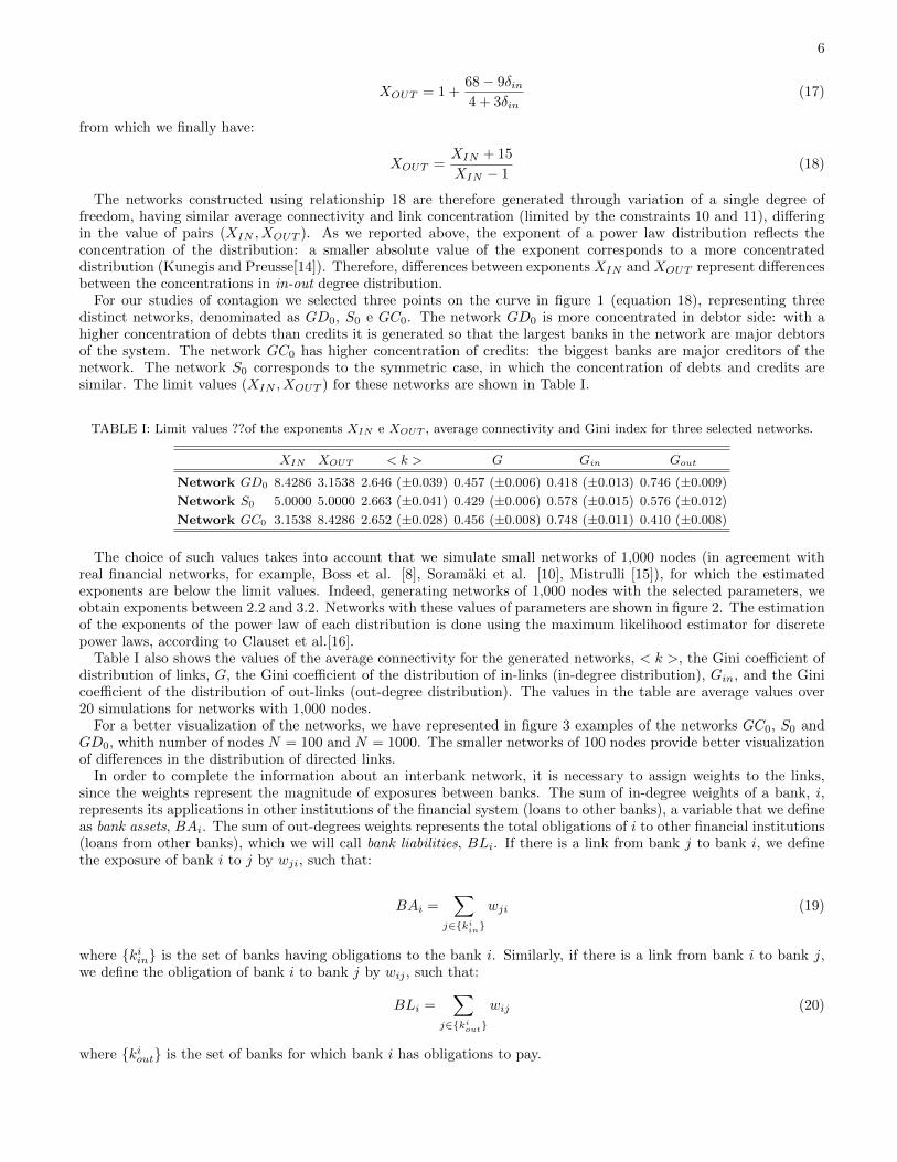
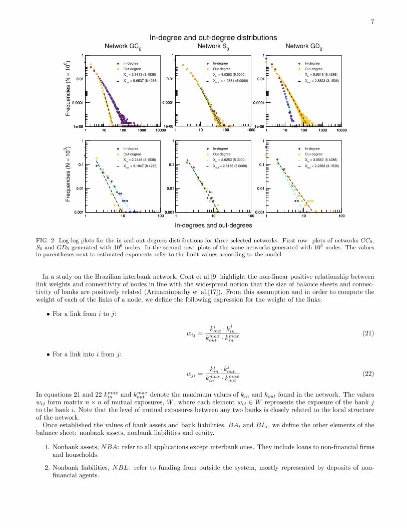
The choice of such values takes into account that we simulate small networks of 1,000 nodes (in agreement withreal financial networks, for example, Boss et al. [8], Soramaki et al. [10], Mistrulli [15]), for which the estimatedexponents are below the limit values. Indeed, generating networks of 1,000 nodes with the selected parameters, weobtain exponents between 2.2 and 3.2. Networks with these values of parameters are shown in figure 2. The estimationof the exponents of the power law of each distribution is done using the maximum likelihood estimator for discretepower laws, according to Clauset et al.[16].

Table I also shows the values of the average connectivity for the generated networks, < k >, the Gini coefficient ofdistribution of links, G, the Gini coefficient of the distribution of in-links (in-degree distribution), Gin, and the Ginicoefficient of the distribution of out-links (out-degree distribution). The values in the table are average values over20 simulations for networks with 1,000 nodes.

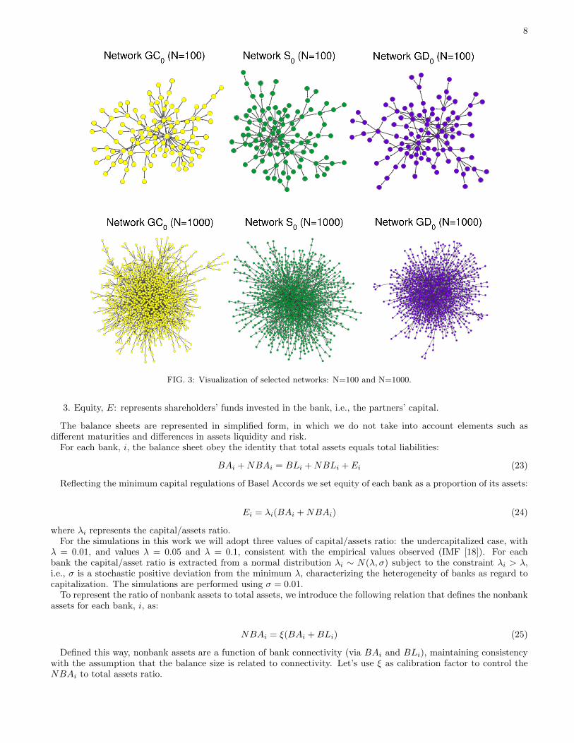
For a better visualization of the networks, we have represented in figure 3 examples of the networks GC0, S0 andGD0, whith number of nodes N = 100 and N = 1000. The smaller networks of 100 nodes provide better visualizationof differences in the distribution of directed links.

In order to complete the information about an interbank network, it is necessary to assign weights to the links,since the weights represent the magnitude of exposures between banks. The sum of in-degree weights of a bank, i,represents its applications in other institutions of the financial system (loans to other banks), a variable that we defineas bank assets, BAi. The sum of out-degrees weights represents the total obligations of i to other financial institutions(loans from other banks), which we will call bank liabilities, BLi. If there is a link from bank j to bank i, we definethe exposure of bank i to j by wji, such that:

BAi =∑

j∈{kiin}

wji (19)

where {kiin} is the set of banks having obligations to the bank i. Similarly, if there is a link from bank i to bank j,we define the obligation of bank i to bank j by wij , such that:

BLi =∑

j∈{kiout}

wij (20)

where {kiout} is the set of banks for which bank i has obligations to pay.

7

1 10 100 1000 100001e-06

0.0001

0.01

1

Frequencies(N

=10

6 )

1 10 100 1000 100001e-06

0.0001

0.01

1

In-degree

Out-degree

Xin = 2.9113 (3.1538)

Xout = 5.6537 (8.4286)

Network GC0

1 10 100 10001e-06

0.0001

0.01

1

1 10 100 10001e-06

0.0001

0.01

1

In-degree

Out-degree

Xin = 4.0362 (5.0000)

Xout = 4.0881 (5.0000)

In-degree and out-degree distributionsNetwork S0

1 10 100 1000 100001e-06

0.0001

0.01

1

1 10 100 1000 100001e-06

0.0001

0.01

1

In-degree

Out-degree

Xin = 5.9516 (8.4286)

Xout = 2.8823 (3.1538)

Network GD0

1 10 1000.001

0.01

0.1

1

Frequencies(N

=10

3 )

1 10 1000.001

0.01

0.1

1

In-degree

Out-degree

Xin = 2.2448 (3.1538)

Xout = 3.1947 (8.4286)

1 10 100

In-degrees and out-degrees

0.001

0.01

0.1

1

1 10 1000.001

0.01

0.1

1

In-degree

Out-degree

Xin = 2.6253 (5.0000)

Xout = 2.6186 (5.0000)

1 10 1000.001

0.01

0.1

1

1 10 1000.001

0.01

0.1

1

In-degree

Out-degree

Xin = 3.0560 (8.4286)

Xout = 2.2363 (3.1538)

FIG. 2: Log-log plots for the in and out degrees distributions for three selected networks. First row: plots of networks GC0,S0 and GD0 generated with 106 nodes. In the second row: plots of the same networks generated with 103 nodes. The valuesin parentheses next to estimated exponents refer to the limit values according to the model.

In a study on the Brazilian interbank network, Cont et al.[9] highlight the non-linear positive relationship betweenlink weights and connectivity of nodes in line with the widespread notion that the size of balance sheets and connec-tivity of banks are positively related (Arinaminpathy et al.[17]). From this assumption and in order to compute theweight of each of the links of a node, we define the following expression for the weight of the links:

• For a link from i to j:

wij =kiout · k

jin

kmaxout · kmax

in

(21)

• For a link into i from j:

wji =kiin · k

jout

kmaxin · kmax

out

(22)

In equations 21 and 22 kmaxin and kmax

out denote the maximum values of kin and kout found in the network. The valueswij form matrix n × n of mutual exposures, W , where each element wij ∈ W represents the exposure of the bank jto the bank i. Note that the level of mutual exposures between any two banks is closely related to the local structureof the network.

Once established the values of bank assets and bank liabilities, BAi and BLi, we define the other elements of thebalance sheet: nonbank assets, nonbank liabilities and equity.

1. Nonbank assets, NBA: refer to all applications except interbank ones. They include loans to non-financial firmsand households.

2. Nonbank liabilities, NBL: refer to funding from outside the system, mostly represented by deposits of non-financial agents.

8

FIG. 3: Visualization of selected networks: N=100 and N=1000.

3. Equity, E: represents shareholders’ funds invested in the bank, i.e., the partners’ capital.

The balance sheets are represented in simplified form, in which we do not take into account elements such asdifferent maturities and differences in assets liquidity and risk.

For each bank, i, the balance sheet obey the identity that total assets equals total liabilities:

BAi +NBAi = BLi +NBLi + Ei (23)

Reflecting the minimum capital regulations of Basel Accords we set equity of each bank as a proportion of its assets:

Ei = λi(BAi +NBAi) (24)

where λi represents the capital/assets ratio.For the simulations in this work we will adopt three values of capital/assets ratio: the undercapitalized case, with

λ = 0.01, and values λ = 0.05 and λ = 0.1, consistent with the empirical values observed (IMF [18]). For eachbank the capital/asset ratio is extracted from a normal distribution λi ∼ N(λ, σ) subject to the constraint λi > λ,i.e., σ is a stochastic positive deviation from the minimum λ, characterizing the heterogeneity of banks as regard tocapitalization. The simulations are performed using σ = 0.01.

To represent the ratio of nonbank assets to total assets, we introduce the following relation that defines the nonbankassets for each bank, i, as:

NBAi = ξ(BAi +BLi) (25)

Defined this way, nonbank assets are a function of bank connectivity (via BAi and BLi), maintaining consistencywith the assumption that the balance size is related to connectivity. Let’s use ξ as calibration factor to control theNBAi to total assets ratio.

9

The identities 23, 24 and 25 form a system of equations by which the value of NBLi can be determined:

NBLi = (1− λi)(1 + ξ)BAi + [(1− λi)ξ − 1]BLi (26)

Thus, the nonbank assets to total assets ratio and the nonbank liabilities to total liabilities ratio are:

NBAi

Ai=

ξ(BAi +BLi)

(ξ + 1)BAi + ξBLi(27)

NBLi

Li=

(1− λi)(1 + ξ)BAi + [(1− λi)ξ − 1]BLi

(1− λi)(1 + ξ)BAi + (1− λi)ξBLi(28)

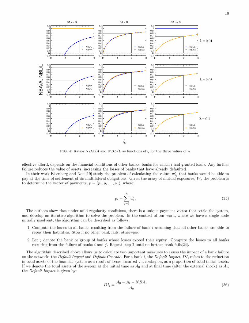
As BAi e BLi are random values (depending on network formation process) we evaluate the equations 27 and 28in three possible limits:

1. BAi � BLi:

NBAi

Ai→ 1 (29)

NBLi

Li→ (1− λi)ξ − 1

(1− λi)ξ(30)

2. BAi = BLi:

NBAi

Ai=

2ξ

2ξ + 1(31)

NBLi

Li=

2ξ(1− λi)− λi2ξ(1− λi)− λi + 1

(32)

3. BAi � BLi:

NBAi

Ai→ ξ

ξ + 1(33)

NBLi

Li→ 1 (34)

Figure 4 shows the ratios 27 and 28 for different values of ξ and for the three values of λ. For the simulations inthis work we fix ξ = 2 in order to obtain balance sheets in which nonbank assets and nonbank liabilities represent onaverage more than 50% of total assets and liabilities.

From the method described in this section we are able to represent the balance sheet of each bank by using onlyinformation from the network and the parameters λ and ξ. In the following section we will describe the cascade offailures following the initial default of one bank of the network.

III. CONTAGION IN INTERBANK NETWORKS: DEFAULT CASCADE AND DEFAULT IMPACT

In this section we present the methodology used to evaluate the propagation of losses in the interbank network.We simulate the insolvency of a single bank, exposed to an external shock represented by the total loss of value of itsnonbank assets. Each bank is tested independently and the impact of its default on the system evaluated.

In a hypothetical scenario a bank, i, becomes insolvent, being unable to completely fulfill its obligations. If attime t, bank j realize that its counterparty i is unable to repay its interbank liability wij in full, then bank j mustreevaluate its application in bank i, from wij to w′ij : (w′ij − wij) < 0. This process adversely affect the capital of j,since variation (w′ij −wij) is incorporated as a loss. It happens that the smaller value, w′ij , the defaulting bank i can

10

0 1 2 3-0.1

00.10.20.30.40.50.60.70.80.9

11.1

0 2

0

NBL/LNBA/A

BA << BL

0 1 2 3-0.1

00.10.20.30.40.50.60.70.80.9

11.1

0

0

NBL/LNBA/A

BA = BL

0 1 2 3-0.1

00.10.20.30.40.50.60.70.80.9

11.1

λ = 0.01

0

0

1

NBL/LNBA/A

BA >> BL

0 1 2 3-0.1

00.10.20.30.40.50.60.70.80.9

11.1

NB

A/A

,NB

L/L

0

0

NBA/ANBL/L

0 1 2 3-0.1

00.10.20.30.40.50.60.70.80.9

11.1

0

0

NBL/LNBA/A

0 1 2 3-0.1

00.10.20.30.40.50.60.70.80.9

11.1

λ = 0.05

0 2

0

NBL/LNBA/A

0 1 2 3-0.1

00.10.20.30.40.50.60.70.80.9

11.1

0 2

0

1

NBL/LNBA/A

0 1 2 3

ξ

-0.10

0.10.20.30.40.50.60.70.80.9

11.1

0

0

NBL/LNBA/A

0 1 2 3-0.1

00.10.20.30.40.50.60.70.80.9

11.1

λ = 0.1

0

0

NBL/LNBA/A

FIG. 4: Ratios NBA/A and NBL/L as functions of ξ for the three values of λ.

effective afford, depends on the financial conditions of other banks, banks for which i had granted loans. Any furtherfailure reduces the value of assets, increasing the losses of banks that have already defaulted.

In their work Eisenberg and Noe [19] study the problem of calculating the values w′ij that banks would be able topay at the time of settlement of its multilateral obligations. Given the array of mutual exposures, W , the problem isto determine the vector of payments, p = (p1, p2, ..., pn), where:

pi =

n∑j=1

w′ij (35)

The authors show that under mild regularity conditions, there is a unique payment vector that settle the system,and develop an iterative algorithm to solve the problem. In the context of our work, where we have a single nodeinitially insolvent, the algorithm can be described as follows:

1. Compute the losses to all banks resulting from the failure of bank i assuming that all other banks are able torepay their liabilities. Stop if no other bank fails, otherwise:

2. Let j denote the bank or group of banks whose losses exceed their equity. Compute the losses to all banksresulting from the failure of banks i and j. Repeat step 2 until no further bank fails[24].

The algorithm described above allows us to calculate two important measures to assess the impact of a bank failureon the network: the Default Impact and Default Cascade. For a bank i, the Default Impact, DIi refers to the reductionin total assets of the financial system as a result of losses incurred via contagion, as a proportion of total initial assets.If we denote the total assets of the system at the initial time as A0 and at final time (after the external shock) as At,the Default Impact is given by:

DIi =A0 −At −NBAi

A0(36)

11

The equation (36) excludes from the computation of DIi the value of Initial Impact (NBAi), representing only thelosses due to contagion. The Total Impact, TIi, is simply the sum of the Initial Impact and the Default Impact:

TIi =NBAi

A0+A0 −At −NBAi

A0(37)

The measure Default Cascade, DCi, refers to the number of insolvent banks due to the failure of bank i, as aproportion of the total number of banks of the network. Both the Default Impact and Default Cascade of a bankreveal how the network would be affected by its failure, taking into account only the direct effects of loss propagationthrough interbank exposures. Although the Default Impact seems the most relevant measure, since it refers to themagnitude of impact in terms of asset value, equally important is the Default Cascade, since the way a crisis is feltby economic agents is also related to the number of affected banks.

To evaluate the sensitivity of contagion to local measures of connectivity and concentration, Cont et al. [9] proposethe indices Counterparty susceptibility, CS(i), and Local network frailty, f(i). Below we reproduce the definitions ofthe authors [9].

Definition (Counterparty susceptibility): The counterparty susceptibility CS(i) of a node i is the maximal (relative)exposure to node i of its counterparties:

CS(i) = maxj

wij

Ej

where Ej is the total exposures of counterparty j.CS(i) is a measure of the maximal vulnerability of creditors of i to the default of i.Definition (Local network frailty): The local network frailty f(i) at node i is defined as the maximum exposure to

node i of its counterparties j (in % of capital of j), weighted by the size of their interbank liability:

f(i) = maxj

wij

EjBLj

As well as the measure CSi, the Local fragility network is a measure of the vulnerability of creditors, but it alsoreflects the sensitivity of indirect lenders of i, represented by the liabilities of counterparty j, BLj .

For the simulations implemented in this paper we calculate the indices CS(i) and f(i) in order to verify therelationship between these topological characteristics and the default impact and defaults cascade of the nodes.

IV. RESULTS

In this section we present the results obtained in contagion simulations for networks produced according to themethodology presented in section II. We have three principal networks as already defined: network GD0 presentsa higher concentration of debts than credits, network GC0 has higher concentration of credits and S0 is symmetric,generated with equal concentrations.

A. Default Impact and Default Cascade

For each set of parameters that defines a network category (GD0, S0 and GC0) we implemented 20 simulations, sothat the analysis is based on 20 realizations of networks of type GD0, 20 realizations of S0 networks and 20 realizationsof GC0 networks. For each generated network and for each bank, i, the Default Impact, DIi and Default Cascade,DCi, were calculated. The results presented in this section are for networks with 1000 nodes, with capital level ofλ = 0.05.

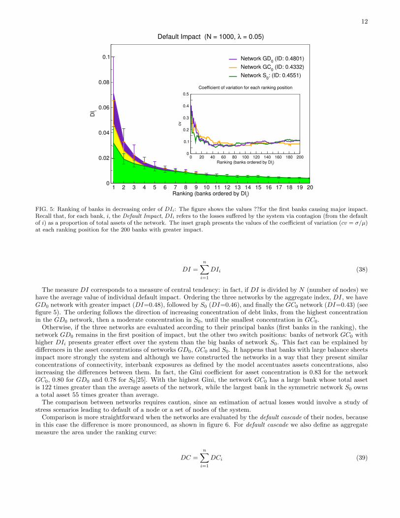
Figure 5 shows the ranking of banks for the three networks, in decreasing order of DIi. The values shown areaverage values for each ranking position, for example, for each network type the greater Default Impact (first rankingposition) is the average of greater impacts for 20 simulations. Equivalently, the subsequent positions of the rankingare average values.

As we can see, the difference between the three types of networks is more pronounced in the first ranking positions,although these positions show greater dispersion around the mean value: in the first position the standard deviationis, for the three categories of networks, around 40% of the average, as shown in the inset graph of Figure 5.

One can consider the area under the ranking curve, which corresponds to the sum of individual impacts, as ameasure of the network systemic risk. We then have for each network an aggregate measure, DI, given by:

12

1 2 3 4 5 6 7 8 9 10 11 12 13 14 15 16 17 18 19 20Ranking (banks ordered by DIi)

0

0.02

0.04

0.06

0.08

0.1

DI i

Network GD0 (ID: 0.4801)Network GC0 (ID: 0.4332)Network S0: (ID: 0.4551)

Default Impact (N = 1000, λ = 0.05)

0 20 40 60 80 100 120 140 160 180 200Ranking (banks ordered by DIi)

0

0.1

0.2

0.3

0.4

0.5

cv

Coefficient of variation for each ranking position

FIG. 5: Ranking of banks in decreasing order of DIi: The figure shows the values ??for the first banks causing major impact.Recall that, for each bank, i, the Default Impact, DIi refers to the losses suffered by the system via contagion (from the defaultof i) as a proportion of total assets of the network. The inset graph presents the values of the coefficient of variation (cv = σ/µ)at each ranking position for the 200 banks with greater impact.

DI =

n∑i=1

DIi (38)

The measure DI corresponds to a measure of central tendency: in fact, if DI is divided by N (number of nodes) wehave the average value of individual default impact. Ordering the three networks by the aggregate index, DI, we haveGD0 network with greater impact (DI=0.48), followed by S0 (DI=0.46), and finally the GC0 network (DI=0.43) (seefigure 5). The ordering follows the direction of increasing concentration of debt links, from the highest concentrationin the GD0 network, then a moderate concentration in S0, until the smallest concentration in GC0.

Otherwise, if the three networks are evaluated according to their principal banks (first banks in the ranking), thenetwork GD0 remains in the first position of impact, but the other two switch positions: banks of network GC0 withhigher DIi presents greater effect over the system than the big banks of network S0. This fact can be explained bydifferences in the asset concentrations of networks GD0, GC0 and S0. It happens that banks with large balance sheetsimpact more strongly the system and although we have constructed the networks in a way that they present similarconcentrations of connectivity, interbank exposures as defined by the model accentuates assets concentrations, alsoincreasing the differences between them. In fact, the Gini coefficient for asset concentration is 0.83 for the networkGC0, 0.80 for GD0 and 0.78 for S0[25]. With the highest Gini, the network GC0 has a large bank whose total assetis 122 times greater than the average assets of the network, while the largest bank in the symmetric network S0 ownsa total asset 55 times greater than average.

The comparison between networks requires caution, since an estimation of actual losses would involve a study ofstress scenarios leading to default of a node or a set of nodes of the system.

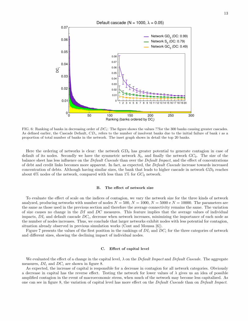
Comparison is more straightforward when the networks are evaluated by the default cascade of their nodes, becausein this case the difference is more pronounced, as shown in figure 6. For default cascade we also define as aggregatemeasure the area under the ranking curve:

DC =

n∑i=1

DCi (39)

13

0 50 100 150 200 250 300Ranking (banks ordered by DCi)

0

0.01

0.02

0.03

0.04

0.05

0.06

0.07

DCi

Network GD0 (DC: 0.99)Network S0 (DC: 0.79)Network GC0 (DC: 0.49)

Default cascade (N = 1000, λ = 0.05)

1 2 3 4 5 6 7 8 9 10 1112 13 14 15 16 17 18 19 200

0.01

0.02

0.03

0.04

0.05

0.06

0.07

0.08

FIG. 6: Ranking of banks in decreasing order of DCi: The figure shows the values ??for the 300 banks causing greater cascades.As defined earlier, the Cascade Default, CDi, refers to the number of insolvent banks due to the initial failure of bank i as aproportion of total number of banks in the network. The inset graph shows in detail the top 20 banks.

Here the ordering of networks is clear: the network GD0 has greater potential to generate contagion in case ofdefault of its nodes. Secondly we have the symmetric network S0, and finally the network GC0. The size of thebalance sheet has less influence on the Default Cascade than over the Default Impact, and the effect of concentrationsof debt and credit links becomes more apparent. In fact, as expected, the Default Cascade increase towards increasedconcentration of debts. Although having similar sizes, the bank that leads to higher cascade in network GD0 reachesabout 6% nodes of the network, compared with less than 1% for GC0 network.

B. The effect of network size

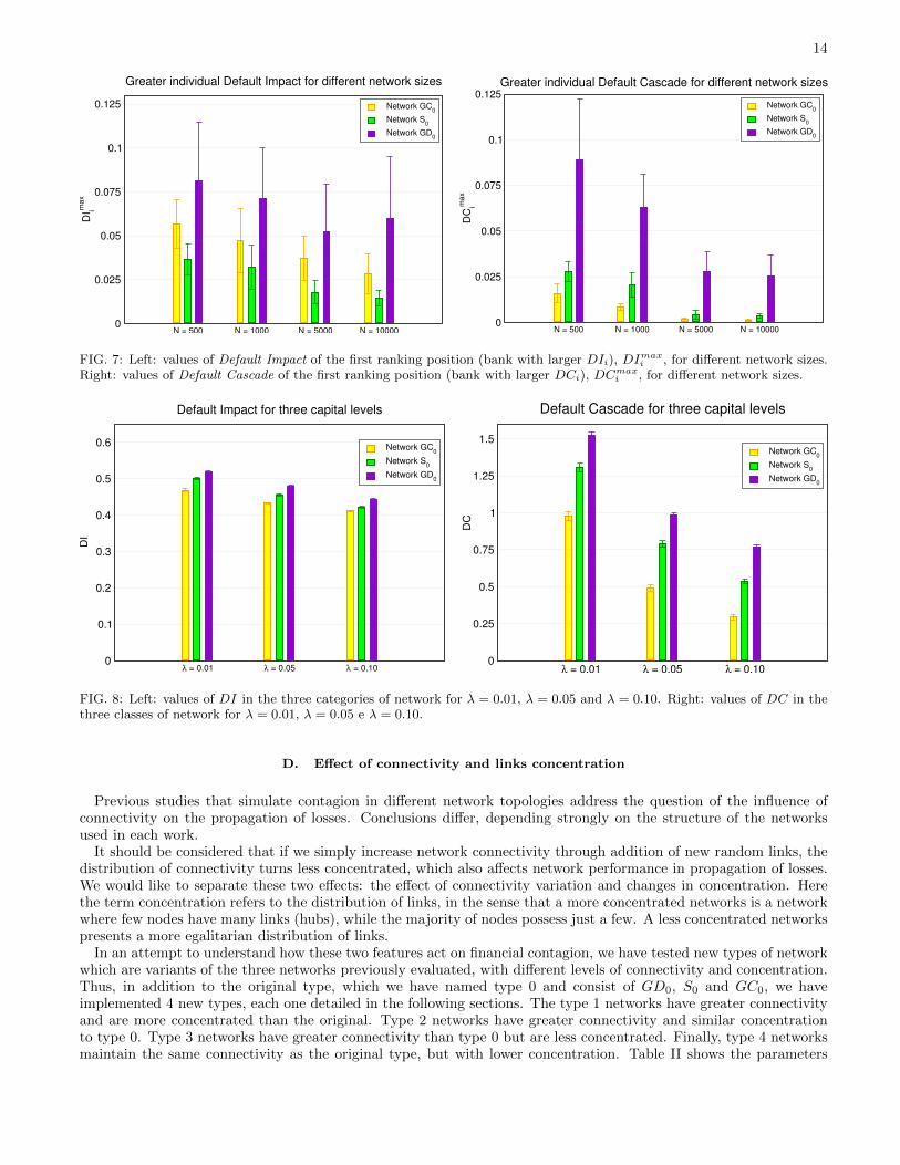
To evaluate the effect of scale on the indices of contagion, we vary the network size for the three kinds of networkanalyzed, producing networks with number of nodes N = 500, N = 1000, N = 5000 e N = 10000. The parameters arethe same as those used in the previous section and therefore the average connectivity remains the same. The variationof size causes no change in the DI and DC measures. This feature implies that the average values of individualimpacts, DIi and default cascade DCi, decrease when network increases, minimizing the importance of each node asthe number of nodes increases. Thus, we conclude that larger networks exhibit nodes with less potential for contagion,situation already observed in previous simulation works (Cont and Moussa [6]).

Figure 7 presents the values of the first position in the rankings of DIi and DCi for the three categories of networkand different sizes, showing the declining impact of individual nodes.

C. Effect of capital level

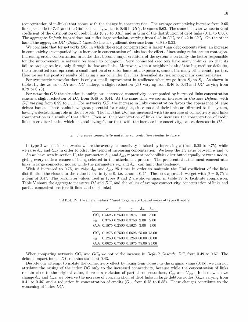
We evaluated the effect of a change in the capital level, λ on the Default Impact and Default Cascade. The aggregatemeasures, DIi and DCi are shown in figure 8.

As expected, the increase of capital is responsible for a decrease in contagion for all network categories. Obviouslya decrease in capital has the reverse effect. Testing the network for lower values of λ gives us an idea of possibleamplified contagion in the event of macroeconomic stress, when much of the network may become less capitalized. Asone can see in figure 8, the variation of capital level has more effect on the Default Cascade than on Default Impact.

14

N = 500 N = 1000 N = 5000 N = 100000

0.025

0.05

0.075

0.1

0.125

DI im

ax

Network GC0

Network S0

Network GD0

Greater individual Default Impact for different network sizes

N = 500 N = 1000 N = 5000 N = 100000

0.025

0.05

0.075

0.1

0.125

DC

imax

Network GC0

Network S0

Network GD0

Greater individual Default Cascade for different network sizes

FIG. 7: Left: values of Default Impact of the first ranking position (bank with larger DIi), DImaxi , for different network sizes.

Right: values of Default Cascade of the first ranking position (bank with larger DCi), DCmaxi , for different network sizes.

λ = 0.01 λ = 0.05 λ = 0.100

0.1

0.2

0.3

0.4

0.5

0.6

DI

Network GC0

Network S0

Network GD0

Default Impact for three capital levels

λ = 0.01 λ = 0.05 λ = 0.100

0.25

0.5

0.75

1

1.25

1.5

DC

Network GC0

Network S0

Network GD0

Default Cascade for three capital levels

FIG. 8: Left: values of DI in the three categories of network for λ = 0.01, λ = 0.05 and λ = 0.10. Right: values of DC in thethree classes of network for λ = 0.01, λ = 0.05 e λ = 0.10.

D. Effect of connectivity and links concentration

Previous studies that simulate contagion in different network topologies address the question of the influence ofconnectivity on the propagation of losses. Conclusions differ, depending strongly on the structure of the networksused in each work.

It should be considered that if we simply increase network connectivity through addition of new random links, thedistribution of connectivity turns less concentrated, which also affects network performance in propagation of losses.We would like to separate these two effects: the effect of connectivity variation and changes in concentration. Herethe term concentration refers to the distribution of links, in the sense that a more concentrated networks is a networkwhere few nodes have many links (hubs), while the majority of nodes possess just a few. A less concentrated networkspresents a more egalitarian distribution of links.

In an attempt to understand how these two features act on financial contagion, we have tested new types of networkwhich are variants of the three networks previously evaluated, with different levels of connectivity and concentration.Thus, in addition to the original type, which we have named type 0 and consist of GD0, S0 and GC0, we haveimplemented 4 new types, each one detailed in the following sections. The type 1 networks have greater connectivityand are more concentrated than the original. Type 2 networks have greater connectivity and similar concentrationto type 0. Type 3 networks have greater connectivity than type 0 but are less concentrated. Finally, type 4 networksmaintain the same connectivity as the original type, but with lower concentration. Table II shows the parameters

15

used in the construction of networks of type 0, 1, 2, 3 and 4.

TABLE II: Parameter values ??used in the construction of networks of type 0, 1, 2, 3 and 4.

α β γ δin δout

GC0 0.5625 0.2500 0.1875 1.00 3.00

S0 0.3750 0.2500 0.3750 2.00 2.00

GD0 0.1875 0.2500 0.5625 3.00 1.00

GC1 0.1875 0.7500 0.0625 1.00 3.00

S1 0.1250 0.7500 0.1250 2.00 2.00

GD1 0.0625 0.7500 0.1875 3.00 1.00

GC2 0.1875 0.7500 0.0625 25.00 75.00

S2 0.1250 0.7500 0.1250 50.00 50.00

GD2 0.0625 0.7500 0.1875 75.00 25.00

GC3 0.5625 0.2500 0.1875 1.00 3.00

S3 0.3750 0.2500 0.3750 2.00 2.00

GD3 0.1875 0.2500 0.5625 3.00 1.00

GC4 0.5625 0.2500 0.1875 10.00 30.00

S4 0.3750 0.2500 0.3750 20.00 20.00

GD4 0.1875 0.2500 0.5625 30.00 10.00

1. Greater connectivity and greater links concentration

In this case we have the networks GD1, S1 and GC1, constructed so that they have greater connectivity and are moreconcentrated than the original ones. This is done by increasing β from 0.25 to 0.75. We maintain the ratio 1:3 betweenα and γ and the same values of δin e δout. As the probability β refers to addition of new link without creation of newnode, increasing β implies increasing the average network connectivity. As the connection mechanism is preferentialattachment, ie nodes that receive links are chosen with probability that is proportional to its previous connectivity,an increase of β also increases links concentration in higher connected nodes, so that the Gini coefficient for linksdistribution increases. Table III shows the aggregate measures, DI and DC, as well as the average connectivity, theGini coefficient for links concentration (G), Gini coefficient for distribution of credit links (Gin) and Gini coefficientfor distribution of debt links.

TABLE III: Aggregate measures, DI and DC, average connectivity, < k >, Gini coefficient for links distribution, G, Ginicoefficient for distribution of credit links, Gin, and Gini coefficient for distribution of debt links, Gout, for network types 0 and1.

DI DC < k > G Gin Gout

GC0 0.433 (±0.001) 0.494 (±0.023) 2.652 (±0.028) 0.456 (±0.008) 0.748 (±0.011) 0.410 (±0.008)

S0 0.455 (±0.004) 0.792 (±0.024) 2.663 (±0.041) 0.429 (±0.006) 0.578 (±0.015) 0.576 (±0.012)

GD0 0.480 (±0.004) 0.988 (±0.015) 2.646 (±0.039) 0.457 (±0.006) 0.418 (±0.013) 0.746 (±0.009)

GC1 0.426 (±0.001) 0.331 (±0.028) 7.406 (±0.166) 0.630 (±0.008) 0.805 (±0.010) 0.561 (±0.010)

S1 0.429 (±0.001) 0.735 (±0.025) 7.484 (±0.227) 0.612 (±0.007) 0.669 (±0.009) 0.671 (±0.008)

GD1 0.437 (±0.002) 1.113 (±0.027) 7.425 (±0.165) 0.630 (±0.008) 0.560 (±0.010) 0.805 (±0.007)

As we see, the increase in average connectivity when accompanied by an increase in the concentration of linkshave different effects depending on the symmetry of the network. As we move from network GC0 to GC1 we see adecrease of contagion effect in response to the increased number of connections and higher concentration of credits

16

(concentration of in-links) that comes with the change in concentration. The average connectivity increase from 2.65links per node to 7.41 and the Gini coefficient, which is 0.46 in GC0, becomes 0.63. The same behavior we see in Ginicoefficient of the distribution of credit links (0.75 to 0.81) and in Gini of the distribution of debt links (0.41 to 0.56).The aggregate Default Impact does not suffer large variation, varying from 0.43 in GC0 to 0.42 in GC1. On the otherhand, the aggregate DC (Default Cascade) has a significant decrease from 0.49 to 0.33.

We conclude that for networks GC, in which the credit concentration is larger than debt concentration, an increasein connectivity accompanied by an increase in concentration of links has the effect of increasing resistance to contagion.Increasing credit concentration in nodes that become major creditors of the system is certainly the factor responsiblefor the improvement in network resilience to contagion. Very connected creditors have many in-links, so that itsfailure propagates less, only through its few out-links. Moreover, when a neighbor bank of the big creditor defaults,the transmitted loss represents a small fraction of creditor bank total exposures, since it has many other counterparties.Here we see the positive results of having a major lender that has diversified its risk among many counterparties.

For symmetric networks there is only a small improvement in resilience when we go from S0 to S1. As shown intable III, the values of DI and DC undergo a slight reduction (DI varying from 0.46 to 0.43 and DC varying from0.79 to 0.73).

For networks GD the situation is ambiguous: increased connectivity accompanied by increased links concentrationcauses a slight reduction of DI, from 0.48 to 0.44. At the same time we see an increase in Cascade Default, withDC varying from 0.99 to 1.11. For networks GD, the increase in links concentration favors the appearance of largedebtor banks. These banks have great potential for contagion, since most of their links are directed to the system,having a destabilizing role in the network. The fact that DC has increased with the increase of connectivity and linksconcentration is a result of that effect. Even so, the concentration of links also increases the concentration of creditlinks in creditor banks, which is a stabilizing factor that, with the increase in connectivity, causes decrease in DI.

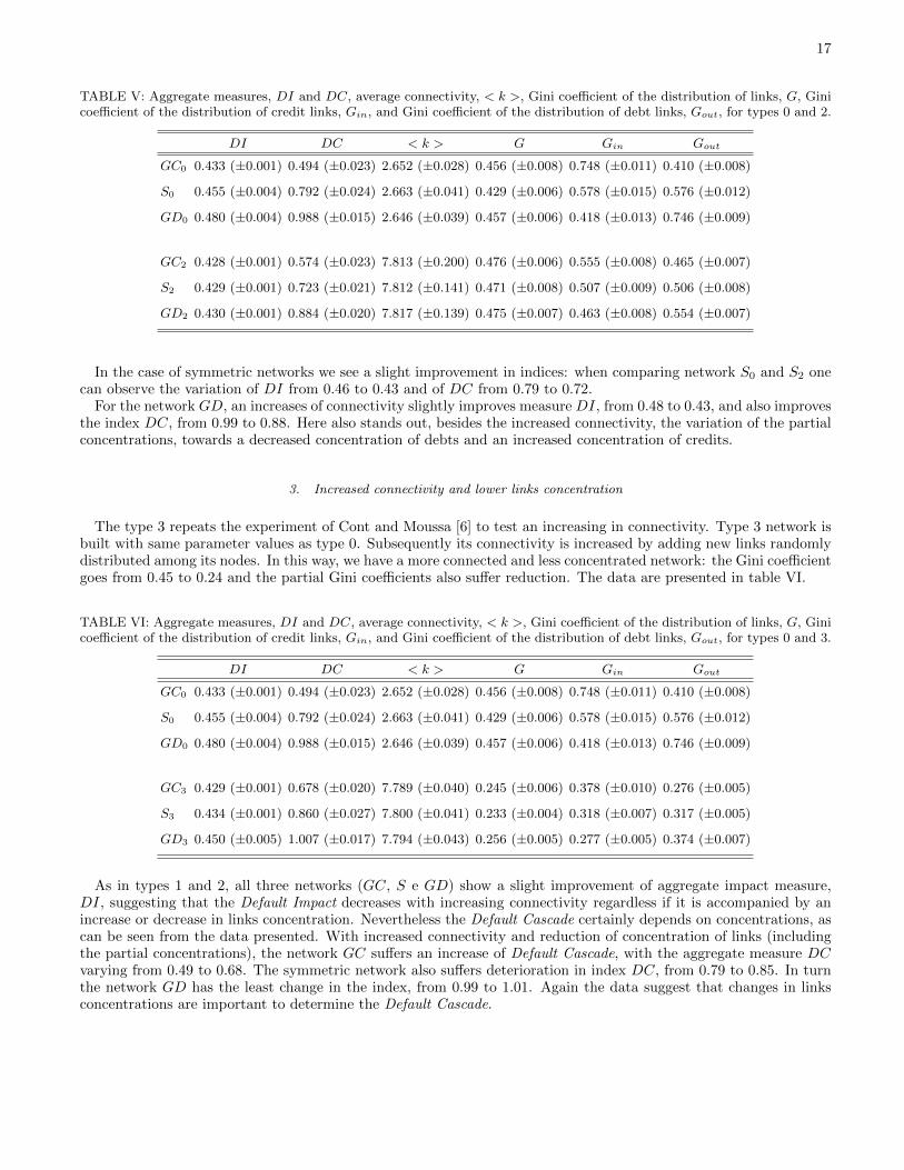
2. Increased connectivity and links concentration similar to type 0

In type 2 we consider networks where the average connectivity is raised by increasing β (from 0.25 to 0.75), whilewe raise δin and δout in order to offset the trend of increasing concentration. We keep the 1:3 ratio between α and γ.

As we have seen in section II, the parameters δin and δout represent probabilities distributed equally between nodes,giving every node a chance of being selected in the attachment process. The preferential attachment concentrateslinks in large connected nodes, while the parameters δin and δout can limit this tendency.

With β increased to 0.75, we raise δin and δout 25 times in order to maintain the Gini coefficient of the linksdistribution the closest to the value it has in type 0, i.e. around 0.45. The best approach we get with β = 0, 75 isa Gini of 0.47. The parameter values used in types 0 and 2 are shown again in table IV to facilitate comparison.Table V shows the aggregate measures DI and DC, and the values of average connectivity, concentration of links andpartial concentrations (credit links and debt links).

TABLE IV: Parameter values ??used to generate the networks of types 0 and 2.

α β γ δin δout

GC0 0.5625 0.2500 0.1875 1.00 3.00

S0 0.3750 0.2500 0.3750 2.00 2.00

GD0 0.1875 0.2500 0.5625 3.00 1.00

GC2 0.1875 0.7500 0.0625 25.00 75.00

S2 0.1250 0.7500 0.1250 50.00 50.00

GD2 0.0625 0.7500 0.1875 75.00 25.00

When comparing networks GC0 and GC2 we notice the increase in Default Cascade, DC, from 0.49 to 0.57. Thedefault impact index, DI, remains stable at 0.43.

Despite our attempt to isolate the connectivity effect by fixing Gini closest to the original value (0.45), we can notattribute the raising of the index DC only to the increased connectivity, because while the concentration of linksremain close to the original value, there is a variation of partial concentrations, Gin and Gout. Indeed, when wechange δin and δout, we observe the increase of concentration of debt links in large debtors nodes (Gout varying from0.41 to 0.46) and a reduction in concentration of credits (Gin from 0.75 to 0.55). These changes contribute to theworsening of index DC.

17

TABLE V: Aggregate measures, DI and DC, average connectivity, < k >, Gini coefficient of the distribution of links, G, Ginicoefficient of the distribution of credit links, Gin, and Gini coefficient of the distribution of debt links, Gout, for types 0 and 2.

DI DC < k > G Gin Gout

GC0 0.433 (±0.001) 0.494 (±0.023) 2.652 (±0.028) 0.456 (±0.008) 0.748 (±0.011) 0.410 (±0.008)

S0 0.455 (±0.004) 0.792 (±0.024) 2.663 (±0.041) 0.429 (±0.006) 0.578 (±0.015) 0.576 (±0.012)

GD0 0.480 (±0.004) 0.988 (±0.015) 2.646 (±0.039) 0.457 (±0.006) 0.418 (±0.013) 0.746 (±0.009)

GC2 0.428 (±0.001) 0.574 (±0.023) 7.813 (±0.200) 0.476 (±0.006) 0.555 (±0.008) 0.465 (±0.007)

S2 0.429 (±0.001) 0.723 (±0.021) 7.812 (±0.141) 0.471 (±0.008) 0.507 (±0.009) 0.506 (±0.008)

GD2 0.430 (±0.001) 0.884 (±0.020) 7.817 (±0.139) 0.475 (±0.007) 0.463 (±0.008) 0.554 (±0.007)

In the case of symmetric networks we see a slight improvement in indices: when comparing network S0 and S2 onecan observe the variation of DI from 0.46 to 0.43 and of DC from 0.79 to 0.72.

For the network GD, an increases of connectivity slightly improves measure DI, from 0.48 to 0.43, and also improvesthe index DC, from 0.99 to 0.88. Here also stands out, besides the increased connectivity, the variation of the partialconcentrations, towards a decreased concentration of debts and an increased concentration of credits.

3. Increased connectivity and lower links concentration

The type 3 repeats the experiment of Cont and Moussa [6] to test an increasing in connectivity. Type 3 network isbuilt with same parameter values as type 0. Subsequently its connectivity is increased by adding new links randomlydistributed among its nodes. In this way, we have a more connected and less concentrated network: the Gini coefficientgoes from 0.45 to 0.24 and the partial Gini coefficients also suffer reduction. The data are presented in table VI.

TABLE VI: Aggregate measures, DI and DC, average connectivity, < k >, Gini coefficient of the distribution of links, G, Ginicoefficient of the distribution of credit links, Gin, and Gini coefficient of the distribution of debt links, Gout, for types 0 and 3.

DI DC < k > G Gin Gout

GC0 0.433 (±0.001) 0.494 (±0.023) 2.652 (±0.028) 0.456 (±0.008) 0.748 (±0.011) 0.410 (±0.008)

S0 0.455 (±0.004) 0.792 (±0.024) 2.663 (±0.041) 0.429 (±0.006) 0.578 (±0.015) 0.576 (±0.012)

GD0 0.480 (±0.004) 0.988 (±0.015) 2.646 (±0.039) 0.457 (±0.006) 0.418 (±0.013) 0.746 (±0.009)

GC3 0.429 (±0.001) 0.678 (±0.020) 7.789 (±0.040) 0.245 (±0.006) 0.378 (±0.010) 0.276 (±0.005)

S3 0.434 (±0.001) 0.860 (±0.027) 7.800 (±0.041) 0.233 (±0.004) 0.318 (±0.007) 0.317 (±0.005)

GD3 0.450 (±0.005) 1.007 (±0.017) 7.794 (±0.043) 0.256 (±0.005) 0.277 (±0.005) 0.374 (±0.007)

As in types 1 and 2, all three networks (GC, S e GD) show a slight improvement of aggregate impact measure,DI, suggesting that the Default Impact decreases with increasing connectivity regardless if it is accompanied by anincrease or decrease in links concentration. Nevertheless the Default Cascade certainly depends on concentrations, ascan be seen from the data presented. With increased connectivity and reduction of concentration of links (includingthe partial concentrations), the network GC suffers an increase of Default Cascade, with the aggregate measure DCvarying from 0.49 to 0.68. The symmetric network also suffers deterioration in index DC, from 0.79 to 0.85. In turnthe network GD has the least change in the index, from 0.99 to 1.01. Again the data suggest that changes in linksconcentrations are important to determine the Default Cascade.

18

4. Same connectivity and lower links concentration

Finally we tested the networks for a decrease in concentration of links, maintaining the same connectivity. We buildnetworks of type 4 by maintaining the same value of β as the original networks, ie, beta = 0.25, and increasing by 10times the values of δin and δout. Parameter values ??are presented in table VII.

TABLE VII: Parameter values ??used to build the networks of types 0 and 4.

α β γ δin δout

GC0 0.5625 0.2500 0.1875 1.00 3.00

S0 0.3750 0.2500 0.3750 2.00 2.00

GD0 0.1875 0.2500 0.5625 3.00 1.00

GC4 0.5625 0.2500 0.1875 10.00 30.00

S4 0.3750 0.2500 0.3750 20.00 20.00

GD4 0.1875 0.2500 0.5625 30.00 10.00

The indices of impact, as well as data connectivity and concentration are shown in table VIII.

TABLE VIII: Aggregate measures, DI and DC, average connectivity, < k >, Gini coefficient of the distribution of links, G,Gini coefficient of the distribution of credit links, Gin, and Gini coefficient of the distribution of debt links, Gout, for types 0and 4.

DI DC < k > G Gin Gout

GC0 0.433 (±0.001) 0.494 (±0.023) 2.652 (±0.028) 0.456 (±0.008) 0.748 (±0.011) 0.410 (±0.008)

S0 0.455 (±0.004) 0.792 (±0.024) 2.663 (±0.041) 0.429 (±0.006) 0.578 (±0.015) 0.576 (±0.012)

GD0 0.480 (±0.004) 0.988 (±0.015) 2.646 (±0.039) 0.457 (±0.006) 0.418 (±0.013) 0.746 (±0.009)

GC4 0.446 (±0.001) 0.714 (±0.016) 2.644 (±0.048) 0.394 (±0.006) 0.608 (±0.009) 0.385 (±0.011)

S4 0.459 (±0.001) 0.871 (±0.022) 2.635 (±0.046) 0.388 (±0.007) 0.509 (±0.009) 0.509 (±0.011)

GD4 0.466 (±0.002) 1.016 (±0.018) 2.661 (±0.036) 0.394 (±0.007) 0.383 (±0.013) 0.607 (±0.010)

For networks GC and S the lowest concentration of links causes worsening of the indices of contagion. For suchnetworks the negative effect of the reduction in concentration of credits is superior to the positive effect of reducingthe concentration of debts.

For networks GD the DI index shows a slight improvement (from 0.48 to 0.46), whereas the index DC has a slightworsening (0.99 to 1.01), indicating that in this case the two effects are balanced.

Figures 9 e 10 summarize the results of this section presenting the values of DI e DC for the 5 types of networkanalyzed.

Comparisons among types suggests that for networks constructed with the algorithm of Bollobas et al. [12] andwith exposures positively related to connectivity, the best scenario is that of a more connected network with highconcentration of credits, featuring large creditors nodes which act as stabilizers of the network. It should be emphasizedagain that in comparisons among network types performed in this work, we do not consider differences among nodesregarding their probabilities of default, differences that can change the evaluation of each network type.

V. CONCLUSIONS

In this paper, we have analyzed the financial contagion via mutual exposures in the interbank market throughsimulations of networks whose degree distributions follows power laws.

We have seen that among the measures of systemic importance (DI and DC), Default Cascade (DC) is the onethat most differentiates the categories of network analyzed. We also observe that, for all categories, both the DefaultImpact and Default Cascade of each node alone does not reach large percentage of the network assets and number

19

Type 0 Type 1 Type 2 Type 3 Type 40

0.1

0.2

0.3

0.4

0.5

DI

Network GCNetwork SNetwork GD

Default Impact (different types of connectivity/concentration)

FIG. 9: Default Impact (aggregate measure) for the 5 types of network analyzed.

Type 0 Type 1 Type 2 Type 3 Type 40

0.25

0.5

0.75

1

1.25

1.5

DC

Network GCNetwork SNetwork GD

Default Cascade (different types of connectivity/concentration)

FIG. 10: Default Cascade (aggregate measure) for the 5 types of network analyzed.

of nodes, respectively. This result is in agreement with the results of stress tests on empirical networks (Upper, C.[20]). Although contagion generated by the failure of an individual node has been shown to be of small amplitude,the differences found among network types may be relevant in the event of market shocks that affect capital of severalinstitutions simultaneously, which would make the system more vulnerable to contagion.

Comparisons among types of network suggest that, for networks whose distributions are close to power laws andexposure is positively related to connectivity, the best scenario is one with a more connected network with highconcentration of credits, featuring large creditors nodes which act as stabilizers of the network. This results suggeststhat the asymmetry observed in distributions of certain real networks is a positive factor, as long as the networkbe more concentrated in distribution of credits (in links). In real networks having power laws exponents estimatedbetween 2 and 3, the results imply that the most stable networks are those with distribution of in links with exponent2 and distribution of out links with exponent 3.

As expected, the increase of capital level reduces contagion in all three categories of network, since the equity ofbanks absorbs impacts suffered by them. We also observed that larger networks have nodes with less potential forcontagion, situation already observed in previous works (Cont and Moussa [6]).

Our simulation shows that the default impact is strongly determined by the initial impact, which was expected,

20

since the assets of large banks (greater initial impact) represent significant portion of the network assets. However,the initial impact does not determines the default cascade to the same extent: default cascade appears to be moresensitive to characteristics of local connectivity.

The results suggest that the size of the balance sheet is the most important factor in determining the impact onassets resulting from the failure of a node, and should not be disregarded or replaced by topological measures thatreflect only information of network connectivity. On the other hand, the network structure has important consequenceson the default cascade. In some cases, the banks which trigger the largest cascades are not the ones with greaterbalance sheet. For those banks, topological measures such as Local network frailty are good indicators of their systemicimportance.

[1] FCIC, Available at http://www.gpo.gov/fdsys/pkg/GPO-FCIC, Financial crisis inquiry commission (2011).[2] F. Allen and A. Babus, Networks in Finance (Pearson Education, 2009), chap. 21.[3] F. Allen and D. Gale, Journal of Political Economy 108, 1 (2000).[4] X. Freixas, B. Parigi, and J.C. Rochet, Journal of Money, Credit and Banking pp. 611-638 (2000).[5] E. Nier, J. Yang, T. Yorulmazer, and A. Alentorn, Journal of Economic Dynamics and Control 31, 2033 (2007).[6] R. Cont and A. Moussa, Financial engineering report, Columbia University (2010).[7] S. Battiston, D. D. Gatti, M. Gallegati, B. Greenwald, and J. E. Stiglitz, Working Paper 15611, National Bureau of

Economic Research (2009)[8] M. Boss, H. Elsinger, M. Summer, and S. Thurner, Quantitative Finance 4, 677 (2004), ISSN 1469-7688, URL

http://www.informaworld.com/10.1080/14697680400020325.[9] R. Cont, A. Moussa, and E. B. e. Santos, Available at SSRN: http://ssrn.com/abstract=1733528 or

http://dx.doi.org/10.2139/ssrn.1733528 (2010).[10] K. Soramaki, M. L. Bech, J. B. Arnold, R. J. Glass, and W. Beyeler, Staff Reports 243, Federal Reserve Bank of New York

(2006), URL http://EconPapers.repec.org/RePEc:fip:fednsr:243.[11] H. Inaoka, T. Ninomiya, K. Taniguchi, T. Shimizu, and H. Takayasu, Bank of Japan working papers 04-E-04, Bank of

Japan (2004).[12] B. Bollobas, C. Borgs, J. T. Chayes, and O. Riordan, in SODA (ACM/SIAM, 2003), pp. 132-139, ISBN 0-89871-538-5,

URL http://dblp.uni-trier.de/db/conf/soda/soda2003.html.[13] A.-L. Barabasi and R. Albert, Science 286, 509 (1999), URL http://www.citebase.org/abstract?id=oai:arXiv.org:cond-

mat/9910332.[14] J. Kunegis and J. Preusse, in Proc. Web Science Conf. (2012), URL http://userpages.uni-koblenz.de/ kunegis/paper/

kunegis-preusse-fairness-on-the-web-alternatives-to-the-power-law.pdf.[15] P. E. Mistrulli, Temi di Discussione, Banca d’Italia, Servizio Studi (2007).[16] A. Clauset, C. R. Shalizi, and M. E. J. Newman, Power-law distributions in empirical data (2007), cite arxiv:0706.1062

Comment: 43 pages, 11 figures, 7 tables, 4 appendices; code available at http://www.santafe.edu/ aaronc/powerlaws/,URL http://arxiv.org/abs/0706.1062.

[17] N. Arinaminpathy, S. Kapadia, and R. May, Bank of England working papers 465, Bank of England (2012), URL http://EconPapers.repec.org/RePEc:boe:boeewp:0465.

[18] IMF, Available at http://fsi.imf.org, Internacional Monetary Fund (2013).[19] L. Eisenberg and T. Noe, Management Science 47, 236 (2001).[20] C.Upper, Journal of Financial Stability 7, 111 (2011), URL http://EconPapers.repec.org/RePEc:eee:finsta:v:7:y:

2011:i:3:p:111-125.[21] H. Elsinger, A. Lehar, and M. Summer, Management Science 52, 1301 (2006).[22] H. M. Ennis, Economic Quarterly 87 (2001).[23] In this work the simulations performed use an initial network, G0, consisted of 2 nodes, 0 and 1, connected by 2 directed

links, 0→ 1 e 1→ 0.[24] For more details about the algorithm see the original paper of Eisenberg and Noe [19].[25] The concentration of assets in real networks is also quite high, as reported in the literature. For example, [21] report a

Gini of 0.88 for the Austrian network in 2002 and [22] reports a Gini of 0.90 for the United States in 2000.