Embed Size (px)
Citation preview

I
I •
I
I
ARMY RESEARCH LA BORA TORY
ARL-MR-200
Assessing the Feasibility of Accelerometer-Only
Inertial Measurement Units for Artillery Projectiles
Thomas E. Harkins
November 1994
APPROVED FOR PUBUC RELEASE; DISTRIBliTION IS UNIJMITED.
I_ .. ··------- --- -

NOTICES
Destroy this report when it is no longer needed. DO NOT return it to the originator.
Additional copies of this report may be obtained from the National Technical Information Service, U.S. Department of Commerce, 5285 Port Royal Road, Springfield, VA 22161.
The findings of this report are not to be construed as an official Department of the Army position, unless so designated by other authorized documents.
The use of trade names or manufacturers' names in this report does not constitute endorsement of any commercial product.

REPORT DOCUMENTATION PAGE Form Approved
OMS No. 0704-0188
PuDI•c reoorttng burden for tl"'l'!l collect• on of 1nformat•on ~~ esttmateac to a.terage- ~ ,...our oer resoor-se. rnc1udtng tne ttme tor rev•ew•ng •nstn.:ct1ons. '!learcnmg e:~.tstrng data wurces. gather~ng and mamta1nrng tl'le d.ata needed. and comcletrng anCI rev•e····ong the .:ollect•on of tntormat1on. Seno comments retarding th•s burden estimate or any other asoect of th•s coltect•on of informattc,, rncJud•ng suggest•ons for reauctng tnrs ouraen. to wa~h•ngton Meaoauarters Ser"•ces. D•rec-:orate or tnformat•on Ooerauons and Reports. 1215 Jefferson Oav1s H•ghway, Su•te 1204. Arlington, VA 22202.-4302. and to the Off1ce of Management and Budget, Paperwcr~ Reduct•on ProJect {0704·0188), Washrngton. OC 20503.
1. AGENCY USE ONLY (Leave blank) ~2- REPORT DATE
November 1994 13. REPORT TYPE AND DATES COVERED
Final - January 1994 - June 1994 4. TITLE AND SUBTITLE 5. FUNDING NUMBERS
Assessing the Feasibility of Accelerometer-Only Inertial Measurement Units for Artillery Projectiles
6. AUTHOR(S) PR: 1L 162618AH80
Thomas E. Harkins
7. PERFORMING ORGANIZATION NAME(S) AND ADDRESS(ES) 8. PERFORMING ORGANIZATION
U.S. Army Research Laboratory REPORT NUMBER
ATTN: AMSRL-WT-WB Aberdeen Proving Ground, MD 21 005-5066
9. SPONSORING I MONITORING AGENCY NAME(S) AND ADDRESS(ES) 10. SPONSORING I MONITORING AGENCY REPORT NUMBER
U.S. Army Research Laboratory ATTN: AMSRL-OP-AP-L ARL-MR-200 Aberdeen Proving Ground, MD 21005-5066
11. SUPPLEMENTARY NOTES
12a. DISTRIBUTION I AVAILABILITY STATEMENT 12b. DISTRIBUTION CODE
Approved for public release; distribution is unlimited.
13. ABSTRACT (Maximum 200 words)
Inertial navigation systems estimate velocity and position information from measurements made with inertial instruments. Most often such systems have included accelerometers and gyroscopes. ,.It has been shown analytically that it is possible to obtain the information necessary to determine both linear accelerations and angular motions using only measurements from linear accelerome-ters. An accelerometer-only inertial measurement unit would be an attractive candidate for use on artillery projectiles due to the availability of high-g miniature accelerometers. After including cod-ing to compute acceleration forces at arbitrary locations on the projectile, a computerized trajectory model was used to evaluate the abilities of various configurations of linear accelerometers and processing algorithms to accurately estimate the components of the projectiles' linear and angular motion.
14. SUBJECT TERMS
Projectile guidance, inertial measurement units, accelerometers
17. SECURITY CLASSIFICATION 18. SECURITY CLASSIFICATION 19. SECURITY CLASSIFICATION OF REPORT OF THIS PAGE OF ABSTRACT
UNCLASSIFIED UNCLASSIFIED UNCLASSIFIED NSN 7540-01-280-5500
15. NUMBER OF PAGES
28 16. PRICE CODE
20. LIMITATION OF ABSTRACT
SAR Standard Form 298 (Rev. 2-89) Pr<>scnbe<l by ANSI >td. Z39·18 Z9S·102

INTENTIONALLY LEFT BLANK
ii

TABLE OF CON1ENTS
Page
LIST OF FIGURES ................................................................................................. v
1. INTRODUCTION ................................................................................................... 1
2. LINEAR ACCELERATION OF A POINT ........................................................ 2
2.1 Accelerations Computed in a Body-Fixed System ......................................... 4 2.2 Accelerations Computed in a Plane-Fixed System ......................................... 6 2.3 Transformation of Acceleration Components From Plane-Fixed
to Body-Fixed System ........................................................................................ 8
3. SIMULATION RESULTS ...................................................................................... 11
3.1 Case 1: M483A1 Artillery Projectile .............................................................. 13 3.2 Case 2: 2.75-Inch MK66 Rocket ..................................................................... 15
4. SUMMARY .............................................................................................................. 17
5. REFERENCES ........................................................................................................ 25
DISTRIBUTION LIST ............................................................................................ 27
iii

INTENTIONALLY LEFT BLANK
iv
L_ -
Figure
1.
2.
3.
4.
5.
LIST OF FIGURES
Page
Accelerometer locations and orientations ......................................................... 19
Body-fixed angular velocity components- M483A1 projectile....................... 20
Angular motion estimation errors- M483A1 projectile.................................. 21
Body-fixed angular velocity components - 2.75-in MK66 rocket .................... 22
Angular motion estimation errors- 2.75-in MK66 rocket............................... 23
v

INTENTIONALLY LEFT BLANK
vi

1. INTRODUCTION
The term "inertial navigation" is commonly used in the literature to describe the
process of obtaining velocity and position information from measurements made with
inertial instruments. To accomplish this, an inertial navigation system must contain
four basic conceptual elements: a vector accelerometer, an attitude reference, a
computer, and a clock (Russell 1962). Russell describes each of these elements as
follows (pp. 17-18). A vector accelerometer is a device which measures the
nongravitational acceleration of the platform to which it is aflxed. Oftentimes this
vector is defmed by three orthogonal components, each of which is measured by a
single-degree-of-freedom (linear) accelerometer. The attitude reference gives the
orientation of the accelerometers in the reference frame in which navigation takes
place. Gyroscopes have most often been employed to this end. The computer is the
conceptual element which solves the acceleration equation by calculating gravitational
acceleration, by performing integrations, and by making coordinate transformations as
required. The clock is needed to predict the gravitational field and the location and
orientation of moving external reference frames (e.g., the earth beneath an aircraft).
It has been shown analytically that it is possible to obtain the information
necessary for determining both linear accelerations and angular motions using only
measurements from linear accelerometers (Schuler, Grammatikos, and Fegley 1967).
Efforts are underway to infer the gravity vector from accelerometer measurements.
The goal is to develop signal processing software that can isolate the gravity-induced
component of projectile pitch that is present in intra-atmospheric trajectories.
Because high-g miniature accelerometers are common but gyros are not, a navigation
system which uses only linear accelerometers for inertial measurements would be an
attractive candidate for inclusion in artillery projectiles. Such a system could perhaps
enable such things as autonomous course corrections and/ or, in conjunction with a
telemeter, projectile registration.
As a start in investigating such possibilities, equations for the inertial acceleration
of an arbitrary point on a flight body have been derived in forms appropriate for
inclusion in a computerized six-degree-of-freedom (6dof) trajectory model used at the
U. S. Army Research Laboratory (ARL). This trajectory model, called CONTRAJ
(Hathaway and Whyte 1991), was then modified to allow up to 12 arbitrarily located
3-axis accelerometers on the projectile. Using appropriate configurations of
accelerometer locations and orientations and linear combinations of accelerometer
outputs, the components of projectile linear and angular motion can be estimated.
-1-

Importantly, it was found that the configurations, orientations, and combinations
that successfully estimate the angular motion components for one projectile will
sometimes not work for another projectile with different motion characteristics. Specifically, a methodology employed by Schuler, Grammatikos, and Fegley for
estimating the components of angular velocity failed due to numerical problems when implemented on the M483Al artillery projectile. An alternative approach yielded
accurate estimates demonstrating that accelerometer-only inertial measurement units need to be tailored to the anticipated flight characteristics of the body on which they
will be installed. Appropriate accelerometer configurations and computational
algorithms for use in many Army projectiles can be identified using the computer model developed for this study.
2. LINEAR ACCELERATION OF A POINT
Defme a set of inertially fixed Cartesian axes X 0 Y 0Z 0 with origin 0 0 and unit
vectors T 0 } 0 7t 0 and a second set of Cartesian axes X Y Z with origin 0 and unit
vectors T}7t. Not only may 0 move relative to 0 0 but tbe X YZ axes may rotate as
well. Consider a point H moving relative to both sets of axes. If we denote H's position relative to 0 0 in the X 0 Y 0Z 0 system by if, 0 's position relative to 0 0 in the
X Y Z system by 0, and H 's position relative to 0 in the X Y Z system by f?, then
(1)
and it can be shown (e.g., Page 1952) that inertial velocity and acceleration of H are given by:
(2)
(3)
where w is the angular velocity of the X Y Z system with respect to the X 0 Y 0Z 0
system.
The velocity is the sum of three terms. The first gives the velocity of the origin of
the moving axes. The second is the velocity of H due to the angular velocity w of the
moving axes. The third h;, is the velocity of H relative to 0 as measured in the
moving system.
-2-
l I I

The acceleration is the sum of five terms. The first is the the acceleration of the
origin of the moving axes. The second is the linear acceleration due to the angular
acceleration iJ of the moving axes. The third is the centripetal acceleration due to the
angular velocity w of the moving axes. The fourth is the Corio lis acceleration where
~ is the velocity of H relative to 0 as measured in the moving system. The fifth
term J:: is the acceleration of H relative to 0 as measured in the moving system.
The equations of motion used to compute projectile and rocket trajectories are
usually evaluated in either of two right-handed Cartesian coordinate systems. The
first, called the body-fixed system, has its origin at the center of mass of the flight body
and its X -axis parallel to the downrange axis of symmetry. The Y and Z axes are then
oriented so that the products of inertia vanish. The three axes of this system are called
the principal axes of inertia of the body. As the name implies, this system is tied to the
flight body and translates, orients, and rotates with that body. The second system,
called the plane-fixed system, also has its origin at the center of mass and its X -axis
along the axis of symmetry. However, the Y and Z axes are not fixed to the projectile.
Rather, the Y -axis is constrained so that it lies in the horizontal plane. A mutually
orthogonal Z -axis then completes this system. Body-fixed coordinates are usually
employed for simulating guided flight bodies because the necessary seekers, sensors,
and control mechanisms are fixed to the bodies and most easily described in such a
system. The plane-fixed system eliminates sensitivity of the integration to projectile
roll rate by eliminating the affected component of gravity. For spin-stabilized
projectiles, this choice of coordinate systems can result in significant computer savings
by not requiring the extremely small integration time steps necessary to avoid
smearing of the gravity effect over the roll angle. Though it is possible for a
sufficiently large flight body to have a gravitational gradient within the body,
CONTRAJ assumes a constant field throughout the body. In CONTRAJ, therefore,
the equation of linear motion is tJ = .f + 1 where .f is the nongravitational
acceleration of the center of mass ( c.m .) and 1 is the gravitational acceleration of the
c.m. .A\s also called by some authors the thmst acceleration, sensed acceleration, or
specific force.
In the next two subsections, the derivations of the body-fixed and plane-fixed
system versions of equations (1)-(3) are summarized. In subsection 2.3, the
acceleration components as computed in the plane-fixed system will be rotated into
the body-fiXed system to allow for comparison with the analogous estimates made for
a trajectory computed in the body-fixed system. Uninterested readers may skip these
and continue with section 3 without loss of continuity.
-3-

2.1. Accelerations Computed in a Body-Fixed System.
When computing a trajectory employing the body-fixed coordinate system, the
vectors in equations (1)-(3) can be expressed as:
it = t::.X0T0 +aY ;)0 +aZ 0K0
0~ x-..t Y,-,.+ z -M>k =a z +a 1 +a
...-+h -..t -..t -M>k = ax l + ay 1 + az
w =pf +q} +rlt (4)
--=-+ 0 -..t 0 -..t 0 ~
w=pl +q; +rk ++ 0 -..t 0 -..t 0 -:-4
hm = t::.X l + ay] + az k
..;.=+ 0 0 -..t 0 0 -..t 0 0 ...-+
hm = ax l + ay J + az k
where p and p are the angular velocity and acceleration of the j -k axes about the i
axis, q and q are the velocity and acceleration of the i-k axes about the j axis, and r
and rare the velocity and acceleration of the i-j axes about thek axis.
Making these substitutions in equation (3), forming the cross products, and
collecting terms yields:
+1[(pq +r)ax +(-p2 -r'Jay +(qr-p)az +2(rax-paz) +t::..Y"] (5)
+K[(pr-q)ax +(qr +p)ay +( -p2 -q2)az +2(pay -qA;_) +t::..Z"}
The components of velocity of the c.m. are typically represented in the moving
(X Y Z ) system as u , v , and w. If we assume that H is fixed on the body, .Ax, ay , and
t::.z are nonconstant only if the c.m. is not fixed, as it generally would not be if fuel or
supplies are consumed during the flight. In such a case, it is useful to make the
following substitutions:
(6)
-4-
-------- ~-- -~
l
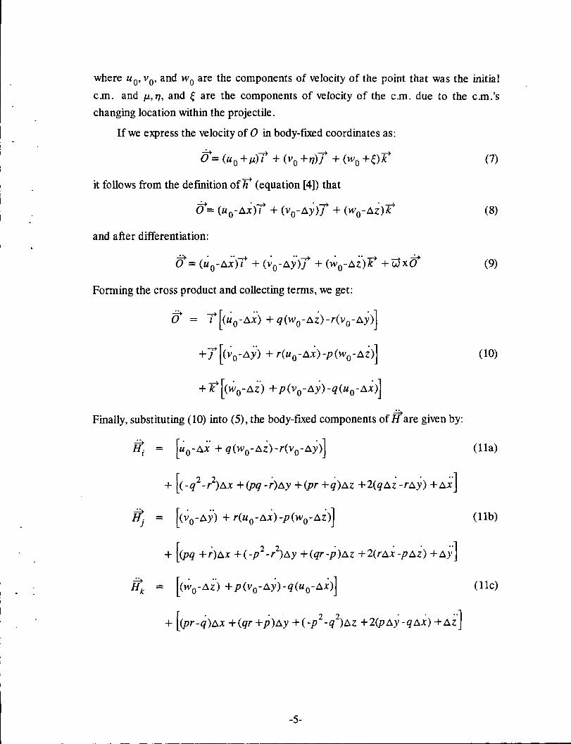
where u0, v0, and w0 are the components of velocity of the point that was the initial
c.m. and Ji., .,, and e are the components of velocity of the c.m. due to the c.m.'s
changing location within the projectile.
If we express the velocity of 0 in body-fixed coordinates as:
a= (uo + p,)f + (vo +.,)} +(wo +€)k
it follows from the defmition of7t (equation [4]) that
and after differentiation:
Forming the cross product and collecting terms, we get:
+ 1[c~0 -6.Y.> + r(u0-6;)-p(w0-6z>]
+ 7( [c~0 -6z.) + p(v0-6y) -q(u0-6;)]
~ Finally, substituting (10) into (5), the body-ftxed components of Hare given by:
H; = [c~0 -6.Y.> + r(u0-6;) -p(w0-6z>]
+ [CPq +r)6x +c -p 2 -r2)6y +(qr-p)6z +2(r6x-p6z) +6.Y·]
-5-
(7)
(8)
(9)
(10)
(lla)
(llb)
(llc)

The body-fixed components of the difference in the accelerations of any two
points H 1 and H 2 are independent of c.m. motion and given by:
~ .. 2 2 . . Hi
1-H;
2 = (-q -r )(~x 1 -~x2) +(pq-r)(~y 1 -~y2) +(pr+q)(~z 1 -~z2) (12a)
.. .. . 2 2 . ~~ -lf12 = (pq +r)(~x 1 -~x2) +( -p -r )(~y 1 -~y2) +(qr-p)(~z 1 -~z2) (12b)
14 -14 = (pr-q)(~x 1 -~x2) +(qr +p)(~y 1 -~y2) +( -p2 -q2)(Az 1-Az2) (12c) I 2
2.2. Accelerations Computed in a Plane-Fixed System.
The plane-fixed coordinate system with its origin at the c.m. differs from the
body-fixed coordinate system with its origin at the c.m. by the angle between the
plane-fixed Y -axis and the body-fiXed Y -axis. This angle will be designated by A¢J, and
the axes of the two systems will be defmed so that they are coincident when ~¢J = 0.
Denoting the distance from the X -axis to H by R and the angle between the Y -axis
and the projection of 0 -H onto the Y -Z plane by ¢J8 , the vectors in equations ( 1)-(3)
can be expressed as:
if= ~X0T0 +~Y ;J0 +~Z 0F0 0-=+ X-;+ Y--;+ Z ....-+k =A l +A ] +A
li = ~x T + R cos if>8 ] + R sin r/>8 7?
--+ --;+ ....-+k w = q] + r ~ ·--;+ • ....-+ w =q] +rk
h; =~xT + (.Rcos¢J8 -Rsin¢J8~8)1 + (.Rsin¢J8 +Rcos¢JH~n) F
-;:: = ~~·--;: + [-R(sin¢J8 (/)8 +cos¢8~~) -2Rsinif>8~8 +Rcos</J8 ]7 + [ R ( cos¢J8 (/)8 - sin<fo8~~) + 2Rcos¢JH~H + R sin<P8 ] 7?
-6-
(13)

Making these substitutions in (3), forming the cross products, and collecting terms yields:
H = ff+f[6.x(-q2 -r2)+Rcos¢H(2q~H-;)+Rsin</JH(2n,{>H +q)
+ Rcos¢H< -2r) +Rsin¢H(2q) +6.~]
+ J[Llx; +6.x(2r) +Rcos</JH( -r2 -~~) + R sin</JH(rq -~H) (14)
+ Rsin</JH( -~H) +Rcos¢H]
+K[Llx( -q) + Llx( -2q) +R cos</JH(qr +~H)+ R sin</JH( -q2 -~~)
+ Rcos¢H<~H) +Rsin¢H]
The most convenient way to reconcile the body-fixed (BF) and plane-fixed (FP)
representations of the location of the point H is to synchronize the two systems initial
conditions. With the coincidence of the two systems (6.¢ = 0), the respective
representations are component-wise equal. With LlxBF =LlxFP' 6.y8F =Rcos¢0,
LlZBF = R sin¢0 initially and denoting the cumulative rotation of the flight body by ¢,
the following relations hold:
<PH= ¢+¢o
~H =~+~o
~H =~+~o
Rcos¢0 = Lly + LlZ~o
Rsin¢0 = LlZ -LlY~o .. .. . 2 . . .. Rcos¢0 = Lly- Lly¢0 +26-z¢0 +Llz¢0
.. .. . 2 . . .. Rsin¢0 = Llz - Llz¢0 - 26-y¢0 - Lly¢0
(15)
~ With these substitutions into (14) and sufficient diligence, the components of H are
then:
~ ~ 2 2 .. H. = 0. +Llx( -q -r) +Llx
I I
+Lly[cos¢(2q¢r,;) +sin¢(2r~+q)] +6.y(2qsin¢-2rcos¢)
+ Llz[cos¢(2r~+q) -sin¢(2q¢r,;)] + 6.Z(2qcos¢ +2rsin¢)
-7-
(16a)
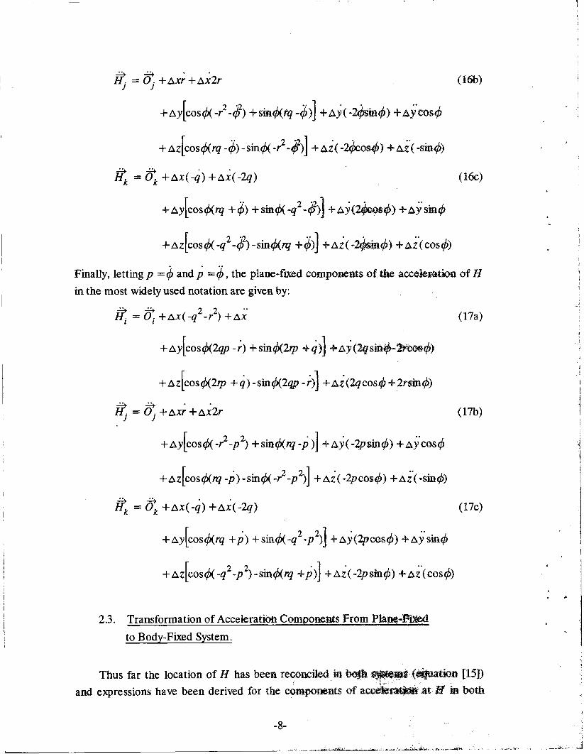
+Ay[cos~ -? -{fh +sm</J(rq -~)] + AY( -2(pgint/J) + Ay.co,s</J
+Az[cos~rq -~)-sin~ -r2 -~1] +Az( -2{pcorfu/>) +Az.( -sinq))
~ =~+Ax( -q) +Ax(-2q)
+Ay[cos¢(rq +~)+sin¢( -q2 -cih] +Ay(~t/>) +Aysinc/J
+ Az[cos~ -q2 -~2) -sinq)(rq +~)) + llZ( -z4>sm</J) + AZ.( cos¢>)
(16b)
(16c)
Finally, letting p = ~ and p = ¢, the plane-fJXed components of the acceler.ation of H
in the most widely used notation are given by:
.. --==+ 22 .. It; = 0 i + .tlX ( -q -r ) + .tlX
+t1y[cos~2qp -;) +sin¢(2rp +q)) +Ay('lqsinfJ-·'l'teoo</>)
+Az[cos¢(2rp +q) -sin¢>{2qp .;)) +Az(2qcost/J+2rsm¢>)
ft. = (j + t1x; + t1x2r 1 1
+lly[cos¢>( -r2 -p2) +sinf/>(rq -p )] +Ay( -2psin</>) +Ay.co~s¢
+ .tlz[cos¢(rq -p) -sin¢>{ -r2 -p2)] + AZ( -2pcosl/J) +Az.( ·sin¢)
~ =~+Ax( -q) +Ax( -2q)
+ Ay[cosif>(rq + p) +sin¢>( -q2 -p2)) + Ay(2poos¢>) + AY. sin</>
+Az[cos~ -q2 -p2)-sin¢>(rq +p)] +Az( -2psin</>) +Az.(cos</>)
2.3. Transformation of Acceleratioo Components From Plane-Pmed
to Body-Fixed System.
(17a)
(17b)
(17c)
Thus far the location of H has been reconciled in·~ ~ (~tion [15])
and expressions have been derived for the components of acc$:rama at B m both
_g,..

systems (equations [11] and [17]). It remains to rotate the components into a common
system. Since strapped-down accelerometers' measurements will be at fixed
orientations with respect to the flight bodies, the plane-fixed components will be
rotated into the body-fixed system using the following:
1
1 0 0 l it . lFP
= 0 cos¢ sin¢ if; 0 -sin,P cos,P [H:J
(18)
Performing the matrix multiplication and equating components gives:
(19a)
i/:1. = i/:
1. cos¢ + ~ sin¢
BF FP FP (19b)
H.k =-it sin¢+Hk cos¢ BF iFP FP
(19c)
After substituting (17) into (19), collecting terms, and employing several trigonometric
identities, the acceleration components in the body-fixed system in terms of the
angular motion components in plane-fixed coordinates are given by:
~ ~ 2 2 .. H. = 0. +~x( -q -r) +~x
lBF l
+ ~y[cos¢<2qp -r) +sin¢<2'P +q)] + ~y(2qsin¢-2rcos¢)
+ ~z[cos¢<2'P +q) -sin¢<2qp -r)] + ~z(2qcos¢ + 2rsin¢)
it. - tf1.cos¢+~sin¢ jBF-
+~x(rcos¢-qsin¢) +~x(2rcos¢-2qsin¢)
2 r +q r -q .. [ ( 2 2] ( 2 2] l +~y -p -
2 -
2 cos2¢+qrsin2¢ +~y
. r -q . [ [ 2 2] l +~z -p +
2 sin2¢ +qrcos2¢ +~z( -2p)
-9-
(20a)
(20b)

J:4BF = tJ; (-sin¢)+ ~(cos¢) (20c)
+Ax( _;sin¢-qcos¢) +Ax( -2rsin¢-2qcos¢)
2 r +q r -q · . .. [ [ 2 2] [ 1 2) ~
+Az -p -2
-2
cos2<f>-qrsin · · +Az
The body-fixed components of the difference in the accelerations of any two
points H 1 and H 2 in terms of the angular motion components in plane·flxed
coordinates are given by:
(2la)
(21b)
2 r +q r -q . . [ [ 2 2) [ 2 2) ~ + -p -
2 -
2 cos2</>+qrsm~ (Ay 1-Ay2)
(21c)
2 r +q r -q [ [ 2 2] [ 2 2] ~ + -p -
2 +
2 cos 2lj>-qrsin2J/> (AZ 1- AZ2)
-10-

3. SIMULATION RESULTS
Though strapped-down linear accelerometers could be installed anywhere on a
projectile and oriented arbitrarily, the algebra required to derive rotational motion
components from the accelerometer measurements is greatly simplified if the
measurement axes of the accelerometers are oriented parallel to the principal axes of
inertia of the projectile (Figure 1). An accelerometer so positioned would be directly
measuring one of the body-fixed components of nongravitational inertial acceleration
at that location. Thus, an accelerometer at Ax, Ay, AZ from the projectile c.m.
oriented in the +f direction would be measuring i/; -8; and similarly for + 1 and +K orientations. When these components are expressed in terms of the linear and
angular motion components in body-ftxed coordinates (equation [11]) and the
difference between the accelerations at two different locations is similarly expressed
(equation [12]), methods for deriving the components of angular velocity and
acceleration can be readily demonstrated.
i/; = [~ 0 -Ax· + q(w0-Az) -r(v0-Ay)]
+ [c -q2 -/)Ax +(pq -r)Ay +(pr +q)Az +2(qAz -rAy) +Ax·]
fi; = [<~0 -Ay.) + r(u 0 -Ax)-p(w0 -Az)]
+ [(pq + r)Ax + ( -p2 -r2)Ay + (qr-p)Az +2(rAx -pAz)+ Ay·]
it. k = [cw0-Az.) + p(v0-Ay)-q(u0-Ax)] ·
+ [(pr-q)~x +(qr+p)~y +(-p2 -q2)~z +2(p~y-q~x) +~z·]
~it. 2 2 . . H.- . = ( -q -r )(~x 1 -Ax2) +(pq -r)(~y 1 -~y2) +(pr +q)(Az 1 -~z2)
11 12
it-it . 2 2 . = (pq +r)(~x 1 -Ax2) +( -p -r )(~y 1 -~y2) +(qr-p)(~z 1 -~z2) 1J h
H.-it. . . 2 2
= (pr-q)(Ax 1 -~x2) +(qr+p)(~y 1 -~y2) +(-p -q )(~z 1 -~z2) kl k2
(lla)
(llb)
(llc)
(12a)
(12b)
(12c)
where p and p are the angular velocity and acceleration of the j -k axes about the i
axis, q and q are the velocity and acceleration of the i-k axes about the j axis, and r
and r are the velocity and acceleration of the i -j axes about the k axis.
-11-

Schuler, Grammatikos, and Fegley postulated a configuration of six
accelerometers positioned as follows:
Ha = LlX +ia, LlY, LlZ
Hb = LlX +')'b' LlY' LlZ
He = LlX, LlY +ic• LlZ
Hd = LlX,LlY +[d,LlZ
He = LlX,Lly,LlZ +ie
Hf = LlX' LlY' LlZ +[!
aligned with the T axis
ali:gned with the r axis
aligned with the 7 axis
aligned· with the 7 axis
aliped with the 7? axis
aligned with the k' axis
Denoting the corresponding sensed accelerations by A a, A b, A c, Ad, A e, and A f, they
obtained:
A a -Ab 2 2 = ( -q -r Hia -')'b)
or
(q2 +r2) Ab-Aa
== - cl (22a)
la -'Yb
similarly
(p2+rl
Ad-Ac == - c2 (22b)
lc-ld
(p2 +q2) Af-Ae
== - c3 (22c)
'Ye-lf
and ultimately
2 -Cl +Cz +C3
p = (23a) 2
2 Cl-Cz+C3
q = (23b) 2
2 Cl +C2-C3
r = (23c) 2
-12-

They point out the sign difficulty in obtaining p, q, and r and suggest that this
"difficulty can be resolved through the use of auxiliary devices that may be less
accurate and less costly than accelerometers." Implementation of this configuration
and computational scheme in a simulated flight of an M483Al artillery projectile
revealed an additional difficulty with this methodology for such projectiles.
3.1. Case 1: M483Al Artillery Projectile.
The M483A1 is a 155-mm-diameter, spin-stabilized projectile that is launched
from a rifled tube with a 1120 twist. When fired from an M 109 howitzer with a 7w
propelling charge, the M483A1 has a launch velocity of 539 m/ sand an initial spin rate
of :::::::174 rps. At 45° launcher elevation, under nominal conditions, this projectile has a
range of :::::::14 km and a flight time of :::::::60s. At impact, the spin rate is :::::::125 rps.
Thus p, whose units are radians/ s, ranges from :::::::1100 rad/ s to :::::::785 rad/ s
(Figure 2a). At the same time, q and r range in magnitude from near zero at launch
to :::::::0.6 rad/ sat impact (Figures 2b and 2c).
Though the Schuler, Grammatikos, and Fegley method for fmding p, q, and r is
analytically correct, it sometimes failed to produce accurate values of q and r for
simulated flights of this projectile due to numerical difficulties. Whereas p is on the
order of magnitude of 103, q and r are on the order of magnitude of 10-1 or less. Thus
there is an at least four orders of magnitude difference between p and q and p and r
and an eight orders of magnitude difference between their squares. Significant figure
limitations then result in estimation errors for the values of q and r due to the Schuler,
Grammatik:os, and Fegley methodology's reliance on accurately determining (p 2 +q2)
and (p2 +r1.
An M483A1 trajectory with launch conditions as described above was computed
with the known values of p, q, and r and their Schuler, Grammatikos, and Fegley
estimates output to a ftle at 0.015-s intervals throughout the flight. Additionally,
estimates of q and r generated using a different combination of accelerometer
positions and a different computational algorithm were output. Within the
CONTRAJ model as implemented on our branch computer, 64 bits are used to
represent reals, 52 bits of which are used for the mantissa, 11 for the exponent, and 1
for the sign. This gives 15 significant figures to the known values of p, q, and r and
the accelerometer outputs.
Figure 3 gives the percentage of the samples for which the errors in the estimates
of q and r exceeded each of four different levels as a function of the number of
-13-

---- - - -
significant figures carried in the computations for both methodologies. Figure 3a gives
the percentages of time that the magnitudes of the error in the estimate of q and r
exceeded 5% of the known magnitudes of q and r. Figure 3b gives the percentages
for which the error magnitudes exceeded 25%, 3c- 50%, and 3d- 100%. The upper
set of curves in each plot is for the errors in the Schuler, Grammatikos, and Fegley
estimates of q and r. Only at 14 and 15 significant ·figures are these estimates
approximately errorless. The curves for the alternative estimates of q and r are
effectively colinear and are seen as the lower curve in each plot. These estimates are
nonzero only for two significant figure computations. In this case, the estimation error
is primarily due to round-off as the estimates are always being compared to the 15
significant figure known values of q and r.
Though this alternative method of estimating angular velocity components has
the advantage of requiring less significant figures in its computations (and
accelerometer data), it has the disadvantage of requiring the output of 10
accelerometers rather than 6. Their configuration is:
Ha = AX,Ay +la•AZ
Hb = Ax,Ay +lb'AZ
He = AX,Ay,Az +ic
Hd = Ax,Ay,Az +id
He= AX +1e,Ay,AZ
H1 =Ax +11 ,Ay,Az
Hg =Ax +!g,Ay,Az
Hh =Ax +ih ,Ay,Az
Hi = AX,Ay +/i.AZ
Hj = Ax,Ay +ij'AZ
aligned with the T axis
aligned with the T axis
aligned with the T axis
aligned with the f axis
aligned with the 1 axis
aligned with the 1 axis
aligned with the k' axis
aligl'led with the k' axis
aligned with the 1 axis
aligned with the 1 axis
If the corresponding sensed accelerations are denoted by A a, A b , A c, Ad, A e, A f, A g,
Ah ,Ai, andAj, then:
Aa-Ab pq-r = - cl (24a)
1a-lb
Ac-Ad pr+q = - c2 (24b)
lc-ld
Ae-Af c3 (24c) pq +r = -
1e-lf
-14-
-- - - - - - - - - - -~ - - - - ~ ~------~~--'-· ~.-~--· --

Ag-Ah pr-q = (24d)
lg-lh
A.-A. p2+r2
I J = (24e)
lj-li
Recalling that p 2
is eight or more orders of magnitude greater than r2, the . . 2 2 2. T .
approxnnauon p z p + r ts made. he estimates of the angular velocity components
are then:
p = vc; (25a)
cl +C3 q = (25b)
zvc; Cz+C4
r = (25c) zvc;
Also readily available are two analytically exact measures of angular acceleration
components:
q = (26a)
r = (26b) 2
3.2. Case 2: 2.75-Inch MK66 Rocket.
The preceding computations were also made for a representative trajectory of
another projectile with very different kinematics, the 2.75-in MK66 rocket. For this
trajectory, the motor was modeled as burning for 1.12 s, at the end of which the
projectile speed was z720 m/ s. When launched at 45° elevation under nominal
conditions, the time of flight was z5Q.6 sand the range to impact was z8050 m. The
known values of the angular velocity components p , q , and r are seen in Figures 4a,
4b, and 4c respectively. For this trajectory, the differences between the order of
magnitude of p 2 and those of q2 and r2 are much less than those seen for the M483Al.
Plotting the percentages for which the estimation errors exceeded the four levels as
-15-

before (Figure 5), the curves for errors in q and r are essentially co1inear for both
methodologies for this projectile. Also, the character of the curves is seen to be like
those for the M483Al albeit at different (lower) values for signifJCant figures. The
Schuler, Grammatikos, and Fegley methodology (upper curves) is outperformed by
the alternative methodology at all levels for computations maintaining less than eight
significant figures. The lower curves, like their counterparts for the M483Al, are
constant valued except for the single instance of two sigWf.teant figures aDGi estimation
errors exceeding 5% . It is not apparent because of the scale, but tile ~nt value is not ::::zero as it was for the M483Al. It is 0.653%. This i.s due to the greater error in h · · f 2 2 2 This . . b lim' d 'f 12 t e approxunat10n o p ::::p + r . approxnnahon can e e . · mate· 1
accelerometers are employed rather than 10. With Ha through Hh, A a through Ah,
and C 1 through C 4 as before, and
Hi = .tt.x,.tt.y,.tt.z +ii
H1 = .tt.x,.tt.y,.tt.z +11 Hk =.tt.x,.tt.y+/k,.tt.z
Ht = .tt.x,.tt.y +it•.tt.z
A.-A. l J
qr-p =
'"Yi-lj
Ak -Az qr+p =
lk -lz
aligned with the 1 axis
aligned with the 1 axis
aligned with the 7( axis
aligned with the k axis
- cs
- c6
The angular velocity components are then given by:
112
p = [(Cl +C3)(C2 +C4)]
2(C5 +C6)
cl +C3 q =
r = 2p
and the angular acceleration components by:
C6-C5 p =
2
(27a)
(27b)
(28a)
(28b)
(28c)
(29a)

q = (29b)
r = (29c) 2
In this methodology, the sign difficulty analytically remains only for p. In practice, this
difficulty appears only for projectiles whose spin direction is either unknown or subject
to reversal during flight. In these instances, an auxiliary sensor could be used to
remove the ambiguity as suggested by Schuler, Grammatikos, and Fegley.
4. SUMMARY
Equations for the inertial acceleration of an arbitrary point on a flight body have
been derived in the two coordinate systems most commonly employed in
computerized trajectory models, the body-fixed and plane-fixed systems. The
equations were constructed in such a form that the location of the point was
reconciled in both systems. The acceleration components in the plane-fixed system
were projected onto the principal inertial axes of the flight body for comparison with
the components as computed in the body-fixed system. Each of the acceleration
components given by these equations represent the sum of the acceleration that will
be measured by a perfect accelerometer located at that point on the flight body whose
measurement axis is oriented parallel to the respective principal axis of inertia and the
projection of the gravity vector onto that axis. The equations for these components
([11] and [17]) further show that these accelerations are given by various combinations
of the translational and angular velocities and accelerations that constitute the body's
kinematics. These equations were included in the CONTRAJ 6dof trajectory model.
By appropriately locating and orienting a collection of accelerometers and forming
linear combinations of their outputs, solutions for the velocity and acceleration
components can be derived.
Implementation of a configuration of accelerometers and a computational
algorithm published in a paper by Schuler, Grammatikos, and Fegley revealed a
further consideration in the design of accelerometer-only inertial measurement
devices. Though the Schuler, Grammatikos, and Fegley method for fmding angular
velocity components is analytically correct, it sometimes failed to produce accurate
estimates of these velocities in a simulated flight of an M483A1 projectile due to
numerical difficulties. The successful estimation of these velocities employing an
alternative approach demonstrated both the necessity of application driven design of
-17-

---------------
such systems and the utility of the accelerometer augmented CONTRAJ model in
such efforts.
Realistic models of accelerometers need to be added to CO NTRAJ as a next
step in investigating the possibility of practical accelerometer-only inertial systems.
How bias, noise, and other corruptions of the 'perfect' acceleration measurements
assumed in this study impact such systems will be the subject of future efforts.
-18-

1111 ACCELEROMETERS
X
z
Figure 1. Accelerometer locations and orientations.
-19-

0 0 -1 -1
0 0 0 <II 0 riJ -1
' '1:) 0 al 0 I. C1l
Po. 0 a ID
g+-----------.---------~~---------~------~---1 r- 0. 15. 30. 45. Time (seo)
a. Angular Velocity (p) of j-k Axes About i Axis
ID
0
M 0 0 <II UJ
' 'tl al ci "'
M Q'
0 I
~ 0 I 0. 15. 30. 45. eo.
Time (seo)
b. Angular Velocity (q) of i-k Axes About j Axis
ID 0
M 0 0 <II UJ
' 'tl l'll ci "'
M
"' 0 J
ID
0 I 0. 15. 20. 45. eo.
Tim.e (sec)
c. Angular Velocity (r) at i-j Axes About k Axis
Figure 2. Body-fixed angular velocit\( gg:npgnents,- M4~~;l ~!·
-20-
I ,I

0 0
c:i 0
.... ....
ID «1
1:'-ID 1:'-
Ql tlll ill .... a 0 «1 ID
tlll ill .... a 0 Ql ID
0 I<
0 I<
Ql Ql
il. ID Cll
il. ID Cll
0 .. 0 I
2. 5. ~0. ~5. 2. 5. ~0. 15. Significant Figure Significant Figures
a. Estimate Error Exceeds 5% b. Estimate Error Exceeds 25%
I 0 N 0 - c:i
0 I .... ....
ID ID 1:'-
Ql tlll ill ....
0 a «1 ID
1:'-Ql tlD ill .... a 0 <D ID
0 I<
0 I<
«1 «1 il. ID il. ID
Cll Cll
o,. ci ., .. 2. 5. ~0. 15. 2. 5. ~0. 15.
Significant Figures Significant Figures
c. Estimate Error Exceeds 50% d. Estimate Error Exceeds 100%
Figure 3. Angular motion estimation errors - M483A 1 projectile.

0 N
0 10
IV ..;
Ill
" "0 al 0
"' ...;
'" 10
0 o. 15. 30. 45. eo.
Time (sec)
a. Angular Velocity (p) of j-k Axes About i Axis
IIJ 0
~ 0 0 IV Ul
" 'd al 0 "'
~ 0" 0
I
aJ 0 I 0. 15. 30. 45. 60.
Time (:sec}
b. Angular Velocity (q) of i-k Axes About j Axis
aJ 0
~ c 0 Cll Ul
' 'd al 0 "'
~
"' 0 I
IIJ 0 I 0. 15. 30. 45. 60.
Time (sec)
c. Angular Velocity (r) of i-j Axes About k Axis
Figure 4. Body-fixed angular velocity comeonents- 2.75·in M~66 rocket.
-22-
-------------- -- ---

0 0 ....
10 ['-
Ill llD tU ..., d 0 Ill 10 (,) I< Ill ll. u'i
Cll
0 ., 2.
I tv 0 w 0 I ....
u'i Ill
['-
llD tU ..., d 0 Ill 10 (,) I< Ill ll. 10
Cll
0 ., 2.
.., 4. 6. a_ 10.
Significant. Figures
a. Estimate Error Exceeds 5%
I 4. 6. a_ 10.
Significant. Figures
c. Estimate Error Exceeds 50%
ci 0 ....
10 ['-
Ill bll tU ..., d 0 Ill 10 (,) I< Ill ll. 10
Cll
0
ci 0 ....
10 ['-
Ill bll tU ..., d 0 Ill 10 (,) .. Ill ll. 10
Cll
0
., 2.
., 2.
4_ a_ Significant. Figures
b. Estimate Error Exceeds 25%
4. 6. Significant. Figures
a_
a_
d. Estimate Error Exceeds 100%
Figure 5. Angular motion estimation errors - 2. 75-in MK66 rocket.
-=--~------ ~--
10.
10.

INTENTIONALLY LEFT BLANK
' '
-24-

5. REFERENCES
Hathaway, W., and R. Whyte. ''CONTRAJ -Control Flight Simulation." Contractor
Report, BRL-CR-657, U.S. Army Ballistic Research Laboratory, March 1991.
Page, L., Introduction To Theoretical Physics. Princeton: D. Van Nostrand, 3d ed.,
1952.
Russell, W. T. 'Theory of Inertial Navigation." Inertial Guidance. Edited by G.R.
Pitman, New York: John Wiley & Sons, pp. 16-46, 1962.
Schuler, A. R., A. Grammatikos, and K. A. Fegley. 'Measuring Rotational Motion
With Linear Accelerometers." IEEE Transactions on Aerospace and Electronic
Systems, vol. AES-3, No.3, May 1967.
-25-

• I
INTENTIONALLY LEFT BLANK
-26-

NO. OF NO. OF COPIES ORGANIZATION COPIES ORGANIZATION
2 ADMINISTRATOR COMMANDER DEFENSE TECHNICAL INFO CENTER US ARMY MISSILE COMMAND ATIN: DTIC-DDA ATIN: AMSMI-RD-CS-R (DOC) CAMERON STATION REDSTONE ARSENAL AL 35898-5010 ALEXANDRIA VA 22304-6145
1 COMMANDER 1 COMMANDER US ARMY TANK-AUTOMOTIVE COMMAND
US ARMY MATERIEL COMMAND ATIN: AMSTA-JSK (ARMOR ENG BR) ATIN: AMCAM WARREN MI 48397-5000 5001 EISENHOWER AVE ALEXANDRIA VA 22333-0001 DIRECTOR
US ARMY TRADOC ANALYSIS COMMAND DIRECTOR ATIN: ATRC-WSR US ARMY RESEARCH LABORATORY WSMR NM 88002-5502 ATIN: AMSRL-OP-SD-TN
RECORDS MANAGEMENT 1 COMMANDANT 2800 POWDER MILL RD US ARMY INFANTRY SCHOOL ADELPHI MD 20783-1145 ATIN: ATSH-WCB-0
FORT BENNING GA 31905-5000 3 DIRECTOR
US ARMY RESEARCH LABORATORY ATIN: AMSRL-OP-SD-TU ABERDEEN PROVING GROUND
TECHNICAL LIBRARY 2800 POWDER MILL RD 2 DIR, USAMSAA ADELPHI MD 20783-1145 A TIN: AMXSY -D
AMXSY -MP/H COHEN 1 DIRECTOR
US ARMY RESEARCH LABORATORY 1 CDR, USA TECOM ATIN: AMSRL-OP-SD-TP/ ATIN: AMSTE-TC
TECH PUBLISHING BRANCH 2800 POWDER MILL RD 1 DIR, USAERDEC ADELPHI MD 20783-1145 ATIN: SCBRD-RT
2 COMMANDER CDR, USACBOCOM US ARMY ARDEC A TIN: AMSCB-CII ATIN: SMCAR-TDC PICATINNY ARSENAL NJ 07806-5000 1 DIR, USARL
ATIN: AMSRL-SL-1 1 DIRECTOR
BENET LABORATORIES 5 DIR, USARL ATIN: SMCAR-CCB-TL ATIN: AMSRL-OP-AP-L WATERVLIET NY 12189-4050
1 DIRECTOR US ARMY ADVANCED SYSTEMS
RESEARCH AND ANALYSIS OFFICE ATIN: AMSAT-R-NR/MS 219-1 AMES RESEARCH CENTER MOFFETT FIELD CA 94035-1000
27

NO. OF COPIES ORGANIZATION
ABERDEEN PROVING GROUND
19 DIR, USARL ATIN: AMSRL-WT-PB/N GERBER
AMSRL-WT -W !C MURPHY AMSRL-Wf-WA/H ROGERS AMSRL-WT -WB/
FBRANDON TBROWN LBURKE WCLAY WD'AMICO B DAVIS GDURFEE VLEITZKE RMCGEE A THOMPSON
AMSRL-WT-WC/J ROCCHIO AMSRL-WT-WD/A NIILER AMSRL-WT-WE/
TPERKINS J TEMPERLEY
AMSRL-WT-WF/ GHORLEY TKOGLER
..
28

USER EVALUATION SHEET/CHANGE OF ADDRESS
This Laboratory undertakes a continuing effort to improve the quality of the reports it publishes. Your comments/answers to the items/questions below will aid us in our efforts.
1. ARL Report Number -=ARL=-=---=MR.=.:...--=2=0=0 _______ Date of Report _ __,N~o.uv'""e""'m"""b,..er..___.l....,9""'9..:L4 __ _
2. DateReportReceived __________________________ _
3. Does this report satisfy a need? (Comment on purpose, related project, or other area of interest for which the report will be used.) _______________________ _
4. Specifically, how is the report being used? (Information source, design data, procedure, source of ideas, etc.) _______________________________ _
5. Has the information in this report led to any quantitative savings as far as man-hours or dollars saved,
operating costs avoided, or efficiencies achieved, etc? If so, please elaborate. ---------
6. General Comments. What do you think should be changed to improve future reports? (Indicate
changes to organization, technical content, format, etc.)-----------------
Organization
CURRENT Name ADDRESS
Street or P.O. Box No.
City, State, Zip Code
7. If indicating a Change of Address or Address Correction, please provide the Current or Correct address above and the Old or Incorrect address below.
Organization
OLD Name ADDRESS
Street or P.O. Box No.
City, State, Zip Code
(Remove this sheet, fold as indicated, tape closed, and mail.) (DO NOT STAPLE)
--- ·-- -----------------------------------------------

DEPARTMENT OF THE ARMY
OFFICIAL BUSINESS
BUSINESS REPLY MAIL I
FIRST CLASS PERMIT NO 0001, APG, MD .
Postage will be paid by addressee
Director U.S. Army Research Laboratory ATTN: AMSRL-OP-AP-L
Ill Itt
Aberdeen Proving Ground, MD 21005-5066
NO POSTAGE NECESSARY
IF MAILED tNTHE
UNtTED STATES