Embed Size (px)
Citation preview

7 D - R i A 5 -1 - A1 PF lR fi E T I L ' 6 u u -, ki Vh fs tE D U R E F O R T E S T I N G S E P A R TE i / iI FAMILIES OF HYPOTHESES(U) WISCONSIN UNIV-MADISONI MATHEMATICS RESFARCH CENTER W LOH SEP 83 MRC-TSR-2574UNLRSFE RG980C04 / 21 N
EEEEEEEnEI..'..

1.0.
l 1.8
MICROOPY R SOO TES CAR
NAINA URA F TDRS 1963-A~
MRC Technical Summary Report #2574
A PARAMETRIC BOOTSTRAP PROCEDURE FOR
TESTING SEPARATE FAMILIES OF HYPOTHESES
4Wei-Yin Loh
Mathematics Research CenterUniversity of Wisconsin-Madison610 Walnut StreetMadison, Wisconsin 53705
September 1983
(Received August 10, 1983). '
Approved for public releaseDistribution unlimited
Sponsored by
U. S. Army Research Office National Science FoundationP. 0. Box 12211 Washington, DC 20550Research Triangle ParkNorth Carolina 27709
S. .[. - . . -. - . . . - -. ; . - .. - -. - . - . . . _ . . * . . - . . . .. . . - . . - . . . _ . . .

UNIVERSITY OF WISCONSIN - MADISONMATHEMATICS RESEARCH CENTER
A PARAMETRIC BOOTSTRAP PROCEDURE FOR TESTINGSEPARATE FAMILIES OF HYPOTHESES
Wei-Yin Loh
Technical Summary Report #2574
aeptember 1983
ABSTRACT
It is shown that the size of the parametric bootstrap procedure of
Williams (1970) is biased upward. A bias-corrected version is shown to
* be better. The finite-sample performance -of this procedure in examined
and compared with that of Cox's (1961, 1962) test in a number of
examples. In some of these, the proposed test reduces to the
traditional optimal test.
AKS (KOS) Subject Classification: 62F03
Key Words: Parametric bootstrap; Separate families of hypothesisi
Spline; Golden-section search
Work Unit Number 4 - Statistics and Probability
Department of Statistics and Mathematics Research Center, University ofWisconsin-Madison, Madison, WI 53705.
Sponsored by the United States Army under Contract No. DAAG29-80-C-0041. This material is based upon work supported by the NationalScience Foundation under Grant No. MCS-7927062, Mod 2 and by funds fromthe University of Wisconsin Graduate School Research Committee.

SIGNIFICANCE AND EXPLANATION
This paper proposes a procedure for testing non-nested families of
hypotheses which substitutes ray computing power for asymptotic
approximations. Given access to a modern computer, the procedure is
'1 practically universally applicable. Examples illustrating its small-
sample properties are provided, as are theorems on its asymptotic
behavior.
Th epniiiyfrtewrinKn iw xrse ntidecitv.umr iswt 9, n o ihteato fti
report

A PARAMETRIC BOOTSTRAP PROCEDURE FOR TESTINGSEPARATE FAMILIES OF HYPOTHESES
Wei-Yin Loh
1. Introduction.
This paper considers the problem of finding general procedures for
testing separate families of hypotheses, separate in the sense that an
arbitrary member in the null cannot be obtained as a limit of members in
the alternative hypothesis. A fairly general test has been proposed in
two well-known papers by Cox (1961, 1962). It is based on the property
that, subject to regularity conditions, the normalized logarithm of the
ratio of maximized likelihoods behaves asymptotically like a standard
normal random variable.
Specifically, let (X1,*.*,Xn) be a random sample from a
distribution with density h(x) and consider testing the separate
families H0 : h(x) - f(x,O) vs. H : h(x) - g(x,w) where (OW) are
unknown, possibly vector-valued, parameters. Let 8, w be the maximum
likelihood estimates of 8, w respectively and
Tn - n Z log{g(xi,w)/f(xi,O)} 1.1)
Then, under H0 and subject to appropriate regularity conditions (e.g.
White, 1982),
z -12(T n - EATn + N(o, a2(e)) (1.2)
Department of Statistics and Mathematics Research Center, University ofWisconsin-Madison, Madison, WI 53705.
Sponsored by the United States Army under Contract No. DAAG29-80-C-0041. This material is vased upon work supported by the NationalScience Foundation under Grant No. MCS-7927062, Mod. 2 and by funds fromthe University of Wisconsin Graduate School Research Comittee.
.. ° + , • - .. °. -. o . .°.. . . . . . . . .. ..... . . .. . -. .• ., o ° o " " , ° , . ° p , . % 0° ' . . . ° o ° -° " ° . o .° , . . . . • • ° . , . , - . • , .° °

.= • . .,. , .
for some a (2) > 0. In this paper N(U,o 2 denotes the normal
2distribution with mean p and variance a . Under H1 , Z tends to
+ " almost surely. Hence large values of Z are evidence against H0 .
At nominal level a, Cox's (1961, 1962) test, denoted by +Cox,
rejects H0 if Z > z 1a(;), where z a is the N(0,1) a-quantile.
An obviously desirable property of 0X is that the probability
of a type I error, a,, converges to the nominal level as n
increases. However, no study seems to have been done on the asymptotic
behavior of the size of COX
A variant of +Cox' to which it is asymptotically equivalent under
the null hypothesis, has been suggested by Atkinson (1970). However
this was shown to be not always consistent by Pereira (1977). Some
authors have proposed tests based on statistics other than the
likelihood ratio. Epps, Singleton and Pulley (1982) use the empirical
moment generating function, and Shen (1982) and Sawyer (1983) derive
their tests from information theoretic considerations. None of these
tests appear to be superior to the others.
A common feature of the tests is that they all depend on some form
of asymptotic approximation, and so require various regularity
conditions for their validity. In an attempt to obtain a solution to a
problem where such conditions are absent, Williams (1970a,b) considers a
different approach which substitutes raw computing power for
asymptotics. Given the data, Williams (1970) proposes simulating the
distribution of Tn in (1.1) on a computer assuming that e = 0. The
null hypothesis is rejected at the nominal a level if the observed
-2-
-L- -- I- -I--------o.-----.. .-.. --

value of Tn is greater than the (1-a)-quantile of the simulated
distribution. We will call this procedure +PAR since it has been
named aparametric bootstrap* in other contexts by some authors (e.g.
Efron, 1982).
It seems pertinent to remark here that although the idea of using
computer simulation to obtain the critical values of a test statistic is
not widely practised at the present time, there are problems where no
better alternative exists. For example, when the hypotheses represent
location-scale families of distributions, the well-known uniformly most
powerful invariant test statistic is a ratio of multiple integrals whose
null distribution, exact or approximate, is unknown. However it can be
approximated to any desired degree of accuracy by Monte Carlo simulation
quite easily, especially as the null distribution is independent of the
unknown parameters.
One aim in this paper is to compare the finite-sample performance
of #Cox and #PAR' with emphasis on (i) the extent to which the size
of the test, a exceeds the nominal a, and (ii) the power of the
tests. It is shown in section 2 that ci(* A) is never less than a.
In fact, an example is given in section 3 where 1for allI (+PAR)
a and n. We also show that ai(C x ) can be either biased upward or
downward.
To reduce the bias in cS(+PAR ), a simple modification, f,, is
proposed in section 2. It is shown that if under H0, e is a
consistent estimator and the 1 - a quantile of Tn is a sufficiently
smooth function of 8 for each n, then as(f . ) is bounded above by
-3-
Ni V
1 + C for some > 0 which tends to zero as n + -. No explicitn n
conditions on the limiting distributional behavior of Tn are
assumed. Sections 3 and 4 contain examples comparing the different
tests*
4,4
... ,.
.. 4
7,', ' ;.' - " " " . "-'-' "-"- ."-" "-" ' - " " " . - '"" " " .' . " - '""" "'", ' " " "
I . % " . . , . . ,- . . . . ," " . . . ' - . . - . . " • . ' . - . . , , . • ,

2. Improving on
Let Tn be given in (1.1). For each 0, a and n, define the
critical value c(O,a,n) such that
P (Tn > c(O,an)) - a . (2.1)
We assume for simplicity here that Tn is a continuous random
variable. Let c m(a,n) - sup c(Oan). if c (an) is known, the test3 6 K
MT which rejects H0 if Tn > cm(an) is clearly level a. In
fact, under mild regularity assumptions, #LRT is asymptotically
optimal in terms of Bahadur efficiency (see e.g. Bahadur, 1971 or Brown,
1971). This does not, of course, imply that #LMT is necessarily most
powerful level a for finite n.
While c(O,a,n) can be approximated given 0, a and n, by
brute-force computer simulation if necessary, the computation of
c (an) presents a much harder problem. The parametric bootstrapKA
*PA avoids this by having the rejection region: Tn > c(8,a,n).
Notice that since c(ean) 4 c (a,n), #PAR is at least as powerful as
4LRT . Our first theorem shows that this is obtained at a cost.
Theorem 2.1. For all a and n,
all(PAR ) - sup P1 (Tn > c(la,n)) ) a$6
A
Proof. sup P6 (Tn > c(O,a,n)) 0 sup P0 (Tn > c(an)) - a.e e
The bias in the size of #PAR will be reduced if we use a critical
A A
value for Tn that is greater than c(O,a,n). Assuming that e is a
consistent estimator of 0, this can be done in the following way. Let
I (0) be a 100(1-a ) confidence interval for 8 such that both itsn ..
,, '*, , ,. '," , +, , , . , .,...-,,,...-.. ...,-. -........ . . . . . .. . . . . . .... . .... . . . . .... ...... ....... . . . ..... . . .. ., ... .

length and a tend to zero as n tends to infinity. The idea behind* *
the test we will propose is to use c - c(1 ,a,n) as the critical
value of Tn, where e maximizes c(8,a,n) over I (e). of course,
this method is practicable only if 0 is known a priori for all
I (8). Section 3 contains examples where this is the case. For other0
cases, 6 can at best be approximated with an "interval of
uncertainty" (01 ,82), which will contain 6 if it is assumed that
c(O,a,n) is unimodal in I (0). Making this assumption, the standardn
optimum-seeking methods like the Fibonacci and golden-section search can
be used. Given C' > 0, each of these two methods is known to produce
an interval of uncertainty, of length less than C', with a minimum
number of function evaluations; see e.g. Wilde (1964).
To approximate c(6 ,a,n), let I (8) - (81,82) and" * a " * ;
S- -0. suppose first that < 1 < 82 . Then we may assume
without loss of generality that 8 < 81 - C < 62 + £< e2 , because if
this were not true, we could reduce the interval of uncertainty, and
hence C, by continuing the golden-section search. Let m1
* * * *
c(e ,a,n) - c(e - C, a,n) and m2 - cl0 2 + C, a,n) - c(82,a,n), and
define
c (O,a,n) - max {c(O ,a,n) + Imi • ) (2.2)i-1,2
If 0 e 6 for some i - 1,2, we set mi = 0. Denote by * the
test which rejects the null hypothesis if T > c (8,a,n). Ifn
c(,a,n) is sufficiently smooth, an upper bound on the size of *. can
be obtained.
-6-
,2.

.v%
Theorem 2.2.
(ii). Suppose that (a) for each local maximum 8 of c(8,a,n) there
is 8 6(0) > 0 such that c(e,*,n) is concave for 8 e (0-26,e+26)and, (b) with H0-probability one, I (0) contains at most one local
n
'- mxlumof c(O,a,n). Then C;%. ( + U if whenever 6 obtains
and 0 e I (e), we choose c in (2.2) so small that c < 6(e).
Proof. (i). Obvious.
(ii). The assumptions imply that for every 8,
P( rejects H0) C P8 (Tn > c(8,a,n), 8 e In (e))
+ Pee 8 n())
S,+a
n
Both assumptions in part (ii) of the theorem set conditions on the
smoothness of c(B,a,n). Condition (b) is necessary to ensure that the
search does not yield the 'wrong' local maximum. Although the local
maxima {e} are seldom known in advance, the sequential nature of the
search allows the experimenter to plot the points {(6(,C((Ja,n)}
at each stage and decide for himself whether the length C of the
current interval of uncertainty is small enough for stopping. Stopping
at any stage amounts to making assumption (a) of the theorem with
6(0) e C, if there exists 8 in the observed 1 (9).
-7-
21
t>: K

In the above discussion it is assume that c(B,a,n) can be
obtained exactly for any e selected by the search procedure. When
c(9,*,n) has to be estimated by computer simulation, its value will be
subject to Monte Carlo error. However, since this error can be made
arbitraily small by increasing the number of Monte Carlo replicates, we
assume it to be negligible here.
-8-
- 1

3. Some examples permitting analytic solution.
In this section the superiority of #* is demonstrated in som
classical testing problems where analytic solutions are possible.
x mple 3.1. Testing a normal mean.
Let (Xl,...,Xn) be a random sample from N(IA,O2) -2 < j ( -,
2 > 0, and consider testing H0 : N(0,O 2 ) vs. H1 Nll). It is
easily seen from (1.1) that
T - .5(1 + log s-s 2+ )
2xn
where x is the sample mean and 2 the maximum likelihood estimate of
0 Thus *pAR has the rejection region2 -2 2 -
.5(1 + log s - a + x-2) > k 1 _(a)
where k (a) is the a quantile of T whi a obtains. We cana-"n
avoid the evaluation of ka (s) by rewriting the rejection region as
-2 2 -2 2x/B > k'. Now k' being the I - a quantile of x/a, is
" independent of s. So both PAR and * are equivalent to the t-
test, which is uniformly most powerful unbiased. It turns out that
.COX does not exist for this problem because T - E.T is of ordercxn an-1-n and hence the LHS of (1.2) converges to 0 in probability under
H0 .
Example 3.2. Testing a normal variance.
Let (Xi,...,Xn) be a random sample from N(U,a), - < P < ,
2a > 0. We consider testing the following hypotheses.
2 2(a) H : a = 1 vs. H : a , 2
It can be verified that (1.1) gives Tn S2/4 + constant, where s2 is
2the maximum likelihood estimate of a • Since the distribution of Tn
-9-
S ... .: . . . . .-. .- . . ... - . .\ - -*• " -

is independent of P, *PAR and *. are identical, and yield the
uniformly most powerful test.
An easy calculation shows that at the nominal a level,
rejects H0 if
2ns > n-1 + z_{2(n-1))6 (3.1)
The RHS is precisely the two-term Cornish-Fisher expansion for the2 2
(1-a)-quantile X 1 1 of the Xn_1 distribution. Table 3.1 gives
some numerical values of the size of the test, aI(CO), for differentCI OCOX)
values of a and n. Numbers in parentheses give the ratio /. The
entries indicate that (*COX) is biased upward.
Table 3.1. Values of a and aI/a for" I Cox
2 2(H a = vs. H 2)0 1
a 5 10 20 100
.05 .070(1.4) .067(1.34) .064(1.28) .057(1.14)
.01 .032(3.2) .026(2.6) .022(2.2) .016(1.6)
.005 .024(4.8) .018(3.6) .014(2.8) .009(1.8)
2._2
(b) H0: a 1 vs. H 1 1/2.
As in (a), P and *. are both equivalent to the uniformlyPAR
most powerful invariant test which rejects for small s The rejection
region for *Cox is
2 {(2(n-1)) 1 2.(32
ns < n-i z 2 (3.2)
-10-
-
"--?--.';-;-;'-- ..'- . • ... . ... . . . . " . . . . -. -

Table 3.*2 shows that a I Cx in now biased downward; numbers in
parentheses again give (18 /Go* The reason for the many zeros in the
table is because the miS of (3.2) is negative or close to 0 for those
values of a and n.
Table 3.2. Values of as and ai/a for #O
(H0 (Y 1 vs. H1 cy2 .5
a 5 10 20 100
.05 0(0) .009(.18) .024(.48) .040(.8)
.01 0(0) 0(0) 0(0) .005(.5)
.005 0(0) 0(0) 0(0) .002(.4)
2 2(c) H0 :Y 4 1 vs. H1 > 1.
-2 2Let a be the maximum likelihood estimate of ar under His' i
22 ~2 20,1. Then 0 min(s , 1) , CF1 = max(s I1) and
T n- {.5(s -_1) - log s) sgn(s -_1)
2the latter being an increasing function of s . Hence * rejectsPAR
2 > 22H0 at nominal level a if ns 00X which reduces to
ns 2> X2if s 2 1
2 2n > Xn~,~ if a < 1
2Clearly for a-values satisfying Xfl..1,1-a >n, *PAR yields the
uniformly most powerful level a test. This will be the case for the
levels used in practice. Otherwise, * rejects H0 regardless ofPAR0
the data. Therefore

"a if Xn
',-'." aI ( 0pAR )-I - 1Rotherwise
Since for fixed 1/2 < a < 1,
V X 0 (/2) as v m (3.3)V, 1-0
we conclude that PAR is not even asymptotically level a for
a e (.5,1).
^22To derive *,, let the interval with endpoints 0; exp(± n "1'k )n
be a confidence interval for 0 under HO such that k + -, andn
• .'2 k + 0 as n + . The rejection region for * then has the formn
2 22 2 2 1/2ns > 0 xl- 1 where 0 min{s exp(n k ),11. Hence *.*0 X.1- 0 n
rejects H0 if
2 2 2 I/2(ns >X and s exp(n k) 1}.,.:.,n { 2 > X -1,1- n
or
{n exp(-n 2kn) 1 k > X , and a2 exp(n /2k 1
'' Clearly, at the usual levels of a (< 1/2), +* is also uniformly most
*... powerful level a for sufficiently large n. Unlike #PAR however,
(3.3) and the conditions on kn imply that +i C*.) *a as n + w for
all 0 < a < 1.
It is noted that #Co is not valid in the present situation
because the LHS of (1.2) does not converge to a normal distribution.
"_2This is partly due to the fact that ( 1) is not asymptotically
normal (cf. White, 1982).
Similar results to (c) carry over to the problem of testing
H : N(0,1), e < 80 vs. Hi: N(8, 1), e > e . The next example shows0 0 10
at its worst.
-12-
* ...".*
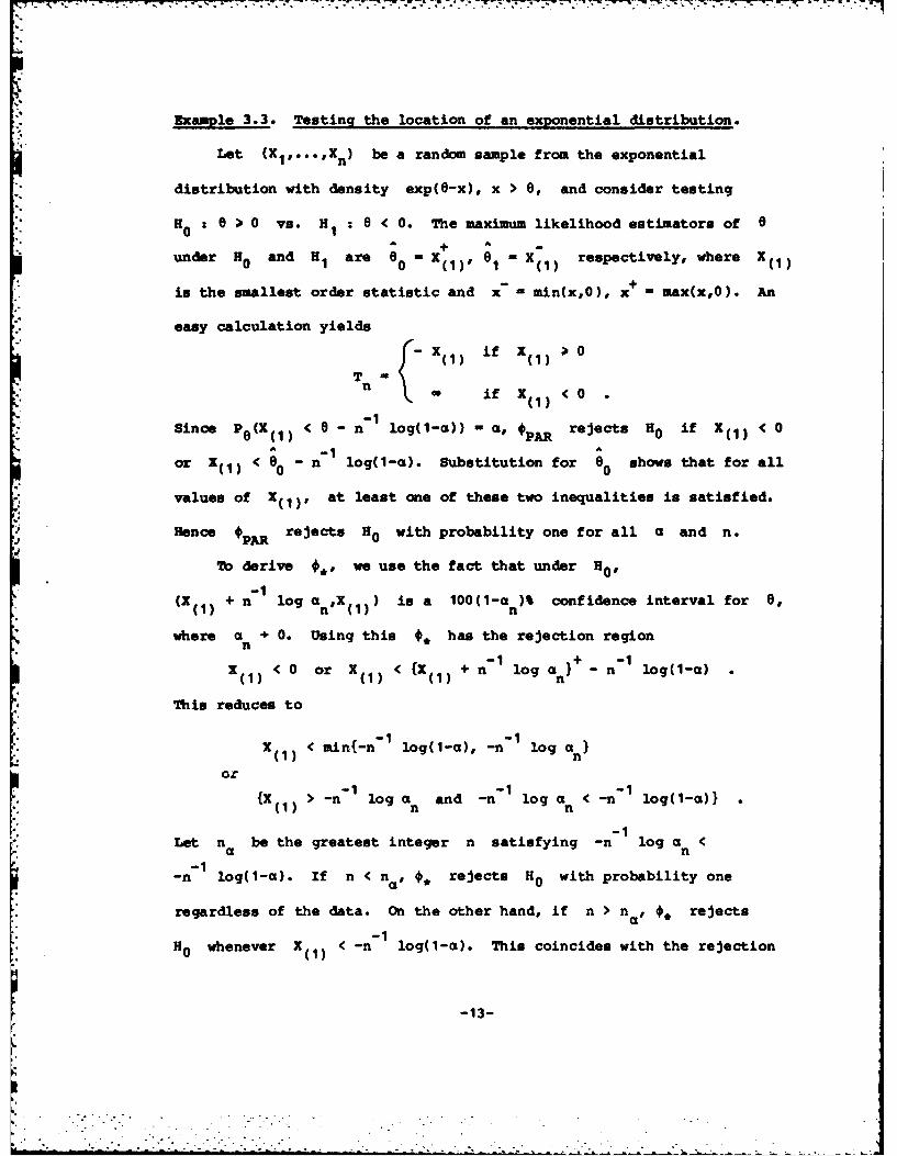
Example 3.3. Testing the location of an exponential distribution.
Let (Xl..*Xn) be a random sample from the exponential
distribution with density exp(O-x), x > 0, and consider testing
H . 0 ) 0 vs. H 8 < 0. The maximum likelihood estimators of 60A + A
under H0 and H1 are ; = -1 1 x 1) respectively, where 1(1)
is the smallest order statistic and x- min(x,O), x - max(x,0). An
easy calculation yields ( -x11 if x1 ) 0
TnT - X(1) i X(1)m if X (1) < 0
Since P8 (( 1 ) < e - n log(I-a)) - a, 0PAR rejects H0 if X(1) < 0
or X11) < 0 - n 1 log1l-a). Substitution for 80 shows that for all
values of X )1, at least one of these two inequalities is satisfied.
Hence +PAR rejects H0 with probability one for all a and n.
To derive *, we use the fact that under H0 ,-1
(X(1) + n log a nX (1 ) is a 100(1-a )% confidence interval for 8,
where a + 0. Using this #* has the rejection regionn -1an}+ -1
X (1) < 0 or X (1) < {X1 + n 1 log a -n n log(l-a)
This reduces to
-1 -1X1) < min{-n - 1 log(l-a), -n log a n
or -1 -1 -1
{X(1) > -n log an and -n "1 log an < -n log(I-a)}* -1
Let na be the greatest integer n satisfying -n log a <a n-1
-n log(1-a). If n < na , 0* rejects H0 with probability one
regardless of the data. On the other hand, if n > na, * rejects-1
H0 whenever X < -n log(l-a). This coincides with the rejection
0
-1 3 -
region of the uniformly most powerful level a teat. Therefore we have
-afor all n > n a and all a. As in part (c) of the earlier
example, * in inapplicable here.Cox
I-14

4. Three examples considered in Cox (1962).
We consider in this section three examples in Cox (1962) where
analytic solutions for the level and power of the tests are not
available. The comparisons are therefore based on Monte Carlo
simulation. Only the nominal level of a - .05 is investigated.
Although the procedure #* as described in section 2 is
computationally quite easy to apply on any one data set, a Monte Carlo
evaluation of its performance using, say, 104 simulated data sets can
be a time consuming task. To reduce this effort, the following
modification of ** is adopted here. In the first stage, after
deciding on the parameter-ranges of interest, a grid of between 20
to 30 8-values is selected. For each selected 8, the critical value
c'(0,*,n) of n/2T is approximated on a computer by simulatingn
10,001 values of n/2 T and setting c°(8,a,n) to be the 9 ,50 1stn
ordered value. The points {(,c'(0,a,n))J are then smoothly
interpolated with a cubic spline to yield an approximation c (e,c,n)
to c'(8,a,n). This curve is stored for use in the second stage, where
for each desired member of the null or alternative hypotheses, 104
sets of pseudo-random samples of size n are simulated. For each set,
the values of n/2 T 8 and the predetermined confidence interval
I (8) are computed. Finally the test ** is said to reject the nulln
hypothesis for that data set if
n 2 T > c (8,a,n) S max{c (8,a,n) : 8 e I (0)) on s n
Note that because ca is a cubic spline, this maximization is quite
trivial. With this modification, the computer evaluation of *, can be
-15-
. -. . .

M done very quickly.
To achieve maximum correlation in the results, the same simulated
data sets were used to assess *Cox The standard errors in the
resulting probabilities of rejection are roughly about .002.
Because #PAR does not permit a similar modification, its
evaluation is included only in Example 4.1. There, for each of 103
." sets of pseudo-random samples, 201 bootstrap samples were simulated to
obtain c'(8,c,n). The standard error of the results for #PAR is
therefore at least .008.
All the computations were done on a VAX 11/750 computer. Pseudo-
random numbers were generated via the International Mathematical and
Statistical Library, and the FORTRAN program in Forsythe, Malcolm and
Moler (1977, Chap. 4) used to fit cubic splines.
Example 4.1. Lognormal versus Exponential.
Let (X,,...,Xn ) be a random sample from a distribution with
density h(x) and consider testing
H : h(x) - f(xiz,) vs. H " h(x) - g(xb)
.4 where x > 0, and
.y )1/ 2 2f f(x,,a) - {xo(2w) exp(-(log x /(2c2)}
g(x,b) - b "1 exp(-x/b) .
Jackson (1968), Atkinson (1970) and Epps, Singleton and Pulley (1982)
have also considered this problem. We will use #ESP to denote the
latter test in the sequel. From Cox (1962), the nominal level a
rejection region for Cox is
S- log X + 2 /2 > n 1/231.(exp( 2 ) - 1 - 2 _ /2} (4.1)
-16-
,, , ,, , " ~~~~~~. . . . .. . . . . . ....... .. .....i ; . .. -. i . ,. ,.. - - .:. ,. . .-.

&2 -1 A2 A £
where a n E(log X 1 - and i -n E log X1 . Also,A A
T nT- log a + p - log X + (log (2w) - 1)/2n
To understand the relative merits of * and #., the following*Cox
remarks may be helpful. First note that the problem is invariant under
scalar multiplication and both #Co and Tn are scale invariant.
Therefore the problem can be reduced by restricting to scale invariant
tests. It can be verified that for each ao, the uniformly most
powerful invariant test of the smaller null hypothesis H' t h(x) -0
f(x,ya 0) vs. H I rejects H' if-1 + A2 2
S(o 0 ) (-) log a0 + a /(2°0) - l I
is too large. Since the LHS of (4.1) is equal to Sn 1 ) , we see that
#COX is an approximation to the uniformly most powerful invariant test
. for 00 - 1. The value a - I is in some sense least favorable because
under H0,
BT + log a -a 2/2 + constant, as n'-
and the limit is maximized at o - 1. On the other hand, T - S (a) .n n
.5 log (2w) - 1 as n + -. Therefore, since #, and P reject for
large values of Tn, they also approximate the uniformly most powerful
invariant test, but by first estimating the unknown o0 with a. These
observations suggest that #CX* , #P and #* would all be reasonable
for large n.
We investigated the performance of these tests by Monte Carlo
simulation for n - 20. Table 4.1 presents the results for the
probability of a type I error, a The figures for # ES P are quoted
from Epps, Singleton and Pulley (1982). Two spline-fitted curves ca
-17-
I.. '" ' : :" : " ":- - :: : : : - : : : : " : " - . . • . . : .i ~

are used, one to obtain the first two rows of Table 4.1, and another for
the remaining rows. The first curve is based on a grid of twenty-five
equally spaced values of log a centered at log(.007). The second
*. curve, shown in Figure 4.1, uses a grid of thirty-one equally spaced
• log a values centered at 0. The spacing of the grid points for both
curves is (2n) / 2 log log n. In the computations for #,, we took the- iinterval with endpoints log ( + (2/n) loglog n as the confidence
interval I (e) for log a. Table 4.2 shows the powers of the fourn
tests. The data indicates that besides having very low power, #Cox has
size in excess of 0.4. *, appears to control the significance level
quite well, with only slight loss of power compared to PAR
Table 4. 1. Prob (Type I error) for H0 : lognormal
vs. H1 : exponential, a - .05, n - 20.
a *ZSPm PAR
0.005 .4056 ? 0 0
0.01 .1229 ? 0 0
0.5 .0172 .066 0 0
1.0 .002 .066 .049 .0206
1.414 .0001 .066 .061 .0497
2.0 .0001 .066 .024 .0127
%t
From Epps, Singleton and Pulley (1982).
-18-

Fig.4.1. Criticalvalues for lognormal vs. Qxpomamrtial
C3
U 0
.010 .3 41 4S
t r m E p , Si g e o n P l e 1 8 )
-19

Tables 4.3 and 4.4 show the corresponding results with the roles of
the hypotheses interchanged. Now PAR and * are the same tests
because the distribution of Tn is invariant over H0 : exponential.
The powers of #Co and f* appear comparable.
Table 4.3. Prob (Type I error) for H0 : exponential
vs. H1 : lognormal, a- .05, n- 20.
#COX 8 P fPAR'+*
.0587 .105 .0517
tFrom Epps, Singleton and Pulley (1982).
Table 4.4. Power of tests for H0 : exponential
vs. H1 : lognormal, a - .05, n - 20.
'! t
#Cox OESP fPA.'O*.10.5 .9999 .9999
1.0 .4014 .22 .3713
1.414 .5482 .60 .5297
2.0 .8951 .8885
From Epps, Singleton and Pulley (1982).
-20-
4 .
• % ,,, . - % . . o .. . . . . . . . .
4-- ° . - . . .* . . . . ...- . ... - 4 - . - ... .- .' '. '. .< -. . . " '. " - " . - .' " -. i- " " • 4 ° . ' " - *" -. "
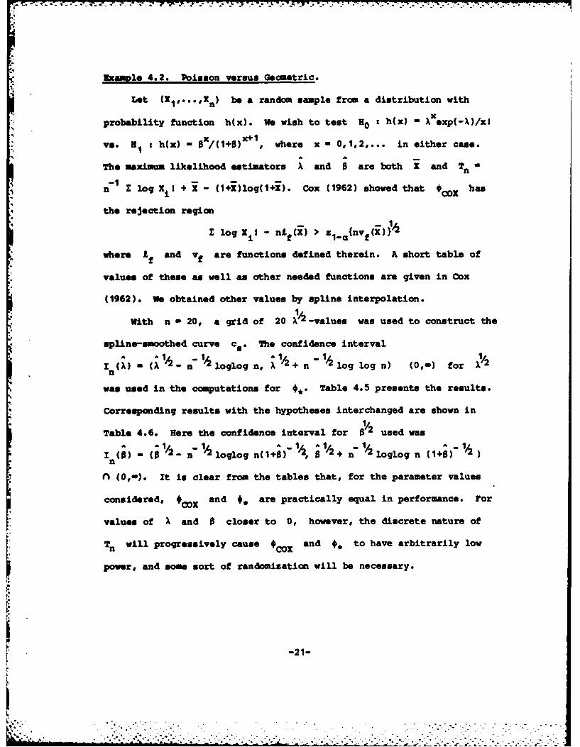
Example 4.2. Poisson versus Geometric.
Let Xi,.**OXn) be a random sample from a distribution with
probability function h(x). We wish to test H0 s h(x) - Xexp(-X)/x!
x x+1vs. H1 a h(x) / B/(1+B)+, where x - 01,2,... in either case.
The maximum likelihood estimators X and 0 are both X and Tn -
-1n I log X i + X - (1+X)log(1+X). Cox (1962) showed that # ox has
the rejection region_I
E log XiI - n fX) > z 1 Q{nvf(X))
where tf and vf are functions defined therein. A short table of
values of these as well as other needed functions are given in Cox
(1962). We obtained other values by spline interpolation.
With n - 20, a grid of 20 X/2-values was used to construct the
spline-smoothed curve c5 s The confidence interval
. ,(., - C - n-"2loglog n 2 .'+ n " log log n) (0, ) for !/2
was used in the computations for *. Table 4.5 presents the results.
Corresponding results with the hypotheses interchanged are shown in
Table 4.6. Here the confidence interval for M/2 used was
/ (2- (/- n " loglog n(1+,o , 1 2+ r- 1/2 loglog n (1+^)-'2n
nl (0,-). It is clear from the tables that, for the parameter values
considered, #Co and #* are practically equal in performance. For
values of A and B closer to 0, however, the discrete nature of
Tn will progressively cause #Co and *, to have arbitrarily low
power, and some sort of randomization will be necessary.
-21-
.4,,* ,,, ~ . - .' ." , - .. .. .- .. . . . . . .. - . -. -. . . .- . - - . •

Table 4.5. Prob (Type I error) and power
for H0 : Poisson vs. H, : Geometric, a- .05, n -20.
Prob (Type I error) Power
"cox ___ _ _cox _ *
.30 .0527 .0309 .30 .199 .156
.45 .0488 .0452 .45 .272 .261
.60 .0478 .0475 .60 .362 .360
.75 .0431 .0427 .75 .453 .450
.90 .0427 .0398 .90 .543 .533
Table 4.6. Prob (Type I error) and power for
H0 : Geometric vs. H, : Poisson, a = .05, n - 20.
8 Prob (Type I error) A Power
#'cox *cox
.30 .0039 .0040 .30 .0185 .0190
.45 .0111 .0137 .45 .0800 .0895
.60 .0182 .0250 .60 .165 .201
.75 .0200 .0315 .75 .254 .321
.90 .0241 .0397 .90 .351 .435
Example 4.3. Quantal response.
Let (X, ...,Xk) be independently binomially distributed with
indices nl,... nk and parameters f1 (Y) ,.••,fk(y) under H0 and
9110I,...,gk(8) under H1, where f (y) 1 -exp(-yxj) and g() =
I - exp(-Oxj) - 8xj.exp(-Oxj) for a set of "dose levels" x
H0 and H1 have been called the "one-hit" and "two-hit" hypotheses
-22-
10 d.
,,', : , .. ". " ... . ..-. . .. . .- .. -. - . -. .. * . . ..

respectively. Following the example in Cox (1962), we chose 5 dose
levels with x1 - .5, x2 - 1, x3 2, x4 - 4 and x5 S 8. Also, we
took n i - 30, i 1
The maximum likelihood estimators y and B were computed
iteratively using the algorithm in Thomas (1972). In the computation
for #* we used as a confidence interval for y the intersection
with (0,-) of the interval with endpoints y t 2 loglog n(ni(y))
where i(Y) - E f (Y)2/{fj(y)(1 _ fj(y))} is the information for Y.
Table 4.7 presents the results of the simulation. Corresponding results
with the hypotheses interchanged are shown in Table 4.8. As in the
preceding example, fCo and ** appear quite comparable, with the
latter keeping the significance level slightly better.
Table 4.7. Prob (Type I error) and power for
H0 : One-hit vs. H1 : Two-hit, a - .05, ni - 30.
y Prob (Type I error) B Power
Ocox f 4co x
.05 .0406 .0474 .10 .252 .327
.10 .0465 .0444 .50 .897 .890
.50 .0436 .0414 1.0 .839 .830
1.0 .0440 .0477 1.5 .704 .696
-23-
iii- i i ~~i 'l~l .~- . . . . . . . . . . ..i 12 '- - -.. . . ..i""i '/ .. . i. .-

Table 4.8. Prob (Type I error) and power for
H0o Two-hit vs. H, One-hit, a .05, n1 30.
B Prob (Type I error) y Power
Ocox 0, cox
.10 .0651 .0478 .05 .724 .677
.50 .0535 .0418 .10 .856 .815
1.0 .0519 .0411 .50 .848 .827
1.5 .0461 .0394 1.0 .645 .634
-24-
5. Concluding remarks.
We have proposed here a test of separate families of hypotheses
which requires very different assumptions from those for tests based on
asymptotic normality of the test statistics, and showed in a series of
examples that it is quite reasonable. The following points however
should be mentioned. First, it is obvious that the results in section 2
remain true if any consistent estimator 8 is used instead of the
maximum likelihood estimator. Further, although these results do not
require conditions on the estimator w in (1.1), it is intuitively
plausible that if high power is to be achieved for *,, w should at
least be consistent. This condition is satisfied in all the examples.
It will be noticed that in the examples, we always have the
critical value c(e,a,n) such that it is either independent of 8 or a
function of a one-dimensional component of 8. In situations where this
is not so, the practical implementation of f, can be difficult, since
we have to search for the maximum of a function in high dimensional
space. In contrast, O does not have the same computationalCoxproblem. However, as we saw in Example 4. 1, the size of fCox may not
be close to its nominal level, and this phenomenon may worsen in higher
dimensions.
Acknowledgement
The author is grateful to Professor E. L. Lehmann for introducing
him to the problem.
-25-

References
1. Atkinson, A. C. (1970). A method for discriminating between models
(with discussion). J. R. Statist. Soc. B 32, 325-353.
2. Bahadur, R. R. (1971). Some limit theorems in statistics.
Philadelphia: Society for Industrial and Applied Mathematics.
3. Brown, L. D. (1971). Non-local asymptotic optimality of
appropriate likelihood ratio tests. Ann. Math. Statist. 42, 1206-
1240.
4. Cox, D. R. (1961). Tests of separate families of hypotheses.
Proc. 4th Berkeley Symp. 1, 105-123.
5. Cox, D. R. (1962). Further results on tests of separate families
of hypotheses. J. R. Statist. Soc. B 24, 406-423.
6. Efron, B. (1982). The Jackknife, the Bootstrap and Other
Resampling Plans. Philadelphia: Society for Industrial and
Applied Mathematics.
7. Epps, T. W., Singleton, K. J. and Pulley, L. B. (1982). A test of
separate families of distributions based on the empirical moment
generating function. Biometrika 69, 391-399.
8. Forsythe, G. E., Malcolm, M. A. and Moler, C. B. (1977). Computer
Methods for Mathematical Computations. Englewood Cliffs, NJ:
Prentice-Hall.
9. Jackson, 0. A. Y. (1968). Some results on tests of separate
families of hypotheses. Biometrika 55, 355-363.
-26-
• • . . o - -... - .

10. Pereira, B. de B. (1977). A note on the consistency and on the
finite sample comparisons of some tests of separate families of
hypotheses. Biometrika 64, 109-113.
11. Sawyer, K. R. (1983). Testing separate families of hypotheses: an
information criterion. J. R. Statiut. Soc. B 45, 89-99.
12. Shen, S. M. (1982). A method for discriminating between models
* describing compositional data. Biometrika 69, 587-595.
13. Thomas, D. G. (1972). Tests of fit for a one-hit vs. two-hit
curve. Appl. Statist. 21, 103-112.
14. White, H. (1982). Regularity conditions for Cox's test of non-
nested hypotheses. J. Econometrics 19, 301-318.
15. Wilde, D. J. (1964). Optimum seeking methods. Englewood Cliffs,
NJ: Prentice-Hall.
16. Williams, D. A. (1970a). Discrimination between regression models
to determine the pattern of enzyme synthesis in synchronous cell
cultures. Biometrics 28, 23-32.
17. Williams, D. A. (1970b). Discussion of Atkinson (1970): A method
for discriminating between models. J. R. Statist. Soc. B 32, 350.
WYL/Jvs
-27-

* SECURITY CLASSIFICATION OF THIS PAGE (11Men Data Enterod)
REOTDCMNAINPAGE READ INSTRUCTIONSREPOR DOCMENTTIONBEFORE COMPLETING FORM1. REORT NMBER2. GOVT ACCESSION NO. S. RECIPIENT'S CATALOG NUMBER
*4. TITLE (dad Subtie) S. TYPE OF REPORT & PERIOD COVERED
A Paramtric Bootstrap Procedure for Testing Sumrprtn R pri osec*Separate Families of Hypotheses 6. PERFORMING ORG. REPORT NUMBER
-7. AUTHOR(s) S. CONTRACT OR GRANT NUMBER(@))ICS-7927062, M~od. 2
* Wei-Yin Loh DAAG29-80-C-00 41
* 9. PERFORMING ORGANIZATION NAME AND ADDRESS 10. PROGRAM ELEMENT PROJECT. TASK
Mathmatcs Rseach ente,, nivesit ofAREA A WORK UNIT NUMBERSMathmatcs Rseach ente, UiverityofWork Unit Number 4 -
610 Walnut Street Wisconsin* ~Madison, Wisconsin 53706 Saitc rbblt
It. CONTROLLING OFFICE NAME AND ADDRESS 12. REPORT CATS
September 1983See Item 18 below 18. NUMBER OF PAGES
1H. MONITORING AGENCY NAME IADDRIESSiI different from Controlling Offace) 1S. SECURITY CLASS. (of this report)
UNCLASSIFIED160. DIECL ASSI FICATION/ DOWNGRADING
SCHEDULE
* I1S. DISTRIBUTION STATEMENT (of tisl Report)
* Approved for public release; distribution unlimited.
- Ii1. DISTRIBUTION STATEMENT (of th. abmtract anltrod ini Block 20. it different *o Ropedt)
* IS. SUPPLEMENTARY NOTESU. S. Army Research Office National Science Foundation
*P. 0. Box 12211 Washington, DC 20550* Research Triangle Park
North Carolina 27709It. KEY WORDS (Conti ot n reveres, aide it necessary and Identify by block aumber)
* Parametric bootstrap; Separate families of hypothesis; Splinie; Golden-section* search.
* 20. ABSTRACT (Canhun aneverse side It necesary ad Identify by black nmmob.,)
* It is shown thac the size of the parametric bootstrap procedure of* William (1970) is I ianed upward. A bias-corrected version is shown to be* better. The finite-saxple performance of this procedure is examined and com-
pared with that of Cox's (1961, 1962) test in a number of examples. In some ofthese, the proposed test reduces to the traditional optimal test.
DD 1473 EDITION OF NOV 65 IS OBSOLETE UNCLASSIFIEDSECURITY CLASSIFICATION OF THIS PAGE (Nhen Data Entered)

V 7~
~~RG,JI
s-
4 .0,
A
9-4
-; ~A 9
f
i.4 -4,
0 9k
17
9.'V.(
7 4W~