i

FINITE ELEMENT METHOD FOR CONSERVED PHASE FIELD MODELS:

SOLID STATE PHASE TRANSFORMATIONS

By

MOHSEN ASLE ZAEEM

A dissertation submitted in partial fulfillment of the requirements for the degree of

DOCTOR OF PHILOSOPHY

WASHINGTON STATE UNIVERSITY School of Mechanical and Materials Engineering

May 2010

ii

To the Faculty of Washington State University:

The members of the Committee appointed to examine the dissertation of

MOHSEN ASLE ZAEEM find it satisfactory and recommend that it be accepted.

Sinisa Dj. Mesarovic, Ph.D. Chair

Hussein M. Zbib, Ph.D.

David P. Field, Ph.D.

Sergey Medyanik, Ph.D.

iii

ACKNOWLEDGEMENTS

First and foremost, I would like to thank my advisor Dr. Sinisa Dj. Mesarovic for

guidance and endless support. I am really blessed to have him as my advisor. Very

special thanks to Dr. Zbib, Dr. Field, and Dr. Medyanik for kindly being on my thesis

committee.

iv

FINITE ELEMENT METHOD FOR CONSERVED PHASE FIELD MODELS:

SOLID STATE PHASE TRANSFORMATIONS

Abstract

By Mohsen Asle Zaeem, Ph.D. Washington State University

May 2010

Chair: Sinisa Dj. Mesarovic Cahn-Hilliard type of phase field model coupled with elasticity equations is used to

derive governing equations for the stress-mediated diffusion and solid state phase

transformations. The partial differential equations governing diffusion and mechanical

equilibrium are of different orders. A mixed-order finite element formulation is

developed, with C0 interpolation functions for displacements, and C1 interpolation

functions for the phase field variable – the concentration. Uniform quadratic

convergence, expected for conforming elements, is achieved for both one and two

dimensional systems.

The developed finite element model (FEM) is used to simulate the nucleation and

growth of the intermediate phase in a thin film diffusion couple as one-dimensional (1D)

problem and the results are compared with Johnson’s finite difference model (FDM).

Two-dimensional (2D) simulations are divided into two categories. In the first category,

2D model is applied to study phase transformations of single precipitates in solid state

binary systems, and the effects of using complete and incomplete Hermite cubic elements

v

on the transformation rate of systems with isotropic and anisotropic gradient energy

coefficients are investigated. In the second category, 2D model is used to study the

stability of multilayer thin film diffusion couples in solid state. Maps of transformations

in multilayer systems are carried out considering the effects of thickness of layers,

volume fraction of films, and compositional strain on the instability of the multilayer thin

films. It is shown that at some cases phase transformations and intermediate phase

nucleation and growth lead to the coarsening of the layers which can result in different

mechanical and materials behaviors of the original designed multilayer.

vi

Dedication

This dissertation is dedicated to

My father: Naser Asle Zaeem

My mother: Tooba Kashan Deghan,

My wife: Sanaz Yazdan Parast

who provided all supports during my study.

vii

TABLE OF CONTENTS

Page

Abstract ................................................................................................................. iv

Dedication .............................................................................................................. vi

TABLE OF CONTENTS...................................................................................... vii

LIST OF FIGURES ............................................................................................... ix

CHAPTER ONE: Introduction ............................................................................................1

1.1 Microstructural Evolution and Phase Field Model ..................................... 1

1.2 Thesis Layout.............................................................................................. 5

CHAPTER TWO: Investigation of Phase Transformation in Thin Film Using Finite

Element Method.......................................................................................................7

2.1 Introduction................................................................................................ 8

2.2 Formulation................................................................................................ 9

2.2.1 Phase field model............................................................................ 9

2.2.2 Equilibrium Conditions................................................................. 12

2.2.3 Diffusion ....................................................................................... 13

2.2.4 Finite element method................................................................... 14

2.3 Results and discussions............................................................................. 16

2.3.1 An equilibrium intermediate phase ( 04.02 −=W ) ........................ 16

2.3.2 Meta-stable intermediate phase ( 01.02 =W ) ................................ 23

2.4 Conclusion ............................................................................................... 26

CHAPTER THREE: Finite element method for conserved phase fields: Stress-

mediated diffusional phase transformation............................................................28

3.1 Introduction.............................................................................................. 29

3.2 Phase field formulation, the weak form................................................... 33

3.2.1 Equilibrium ................................................................................... 34

viii

3.2.2 Diffusion ....................................................................................... 36

3.3 Finite element discretization .................................................................... 39

3.4 Results and discussions............................................................................ 41

3.4.1 Growth of intermediate phase in 1D............................................. 44

3.4.2 Growth of the intermediate phase in 2D – isotropic case ............. 48

3.4.3 Growth of the intermediate phase in 2D – anisotropic case ......... 55

3.5 Conclusions.............................................................................................. 58

Appendix A........................................................................................................... 61

One-dimensional finite element................................................................... 61

Two-dimensional finite element .................................................................. 62

Appendix B ........................................................................................................... 64

CHAPTER FOUR: Morphological Instabilities in Thin Films .........................................66

4.1 Introduction.............................................................................................. 67

4.2 Formulation and Numerical Method........................................................ 69

4.3 Two Phase Multilayer .............................................................................. 75

4.4 Three Phase Multilayer with Stable Intermediate Phase ......................... 78

4.5 Three Phase Multilayer with Meta-Stable Intermediate Phase................ 81

4.6 Conclusion ............................................................................................... 85

CHAPTER FIVE: Summary and Future Works................................................................86

REFERENCES ..................................................................................................................88

ix

LIST OF FIGURES

Page

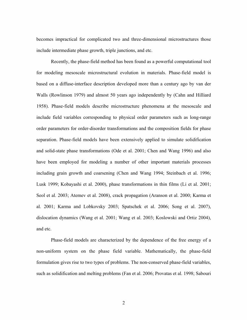
Figure 2.1. Free energy density as a function of composition. The minima are at 5,

50 and 95%. ...........................................................................................................11

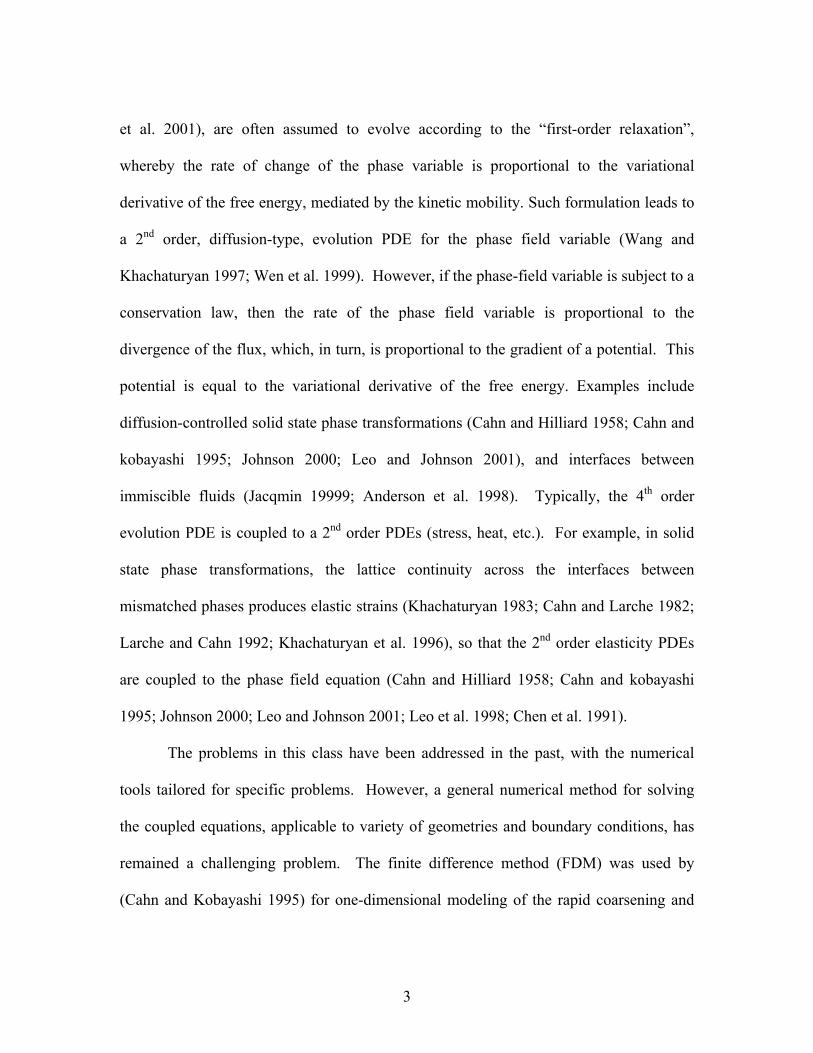
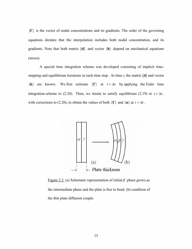
Figure 2.2. (a) Schematic representation of initial β phase grows as the intermediate

phase and the plate is free to bend. (b) condition of the thin plate diffusion

couple. ...................................................................................................................15

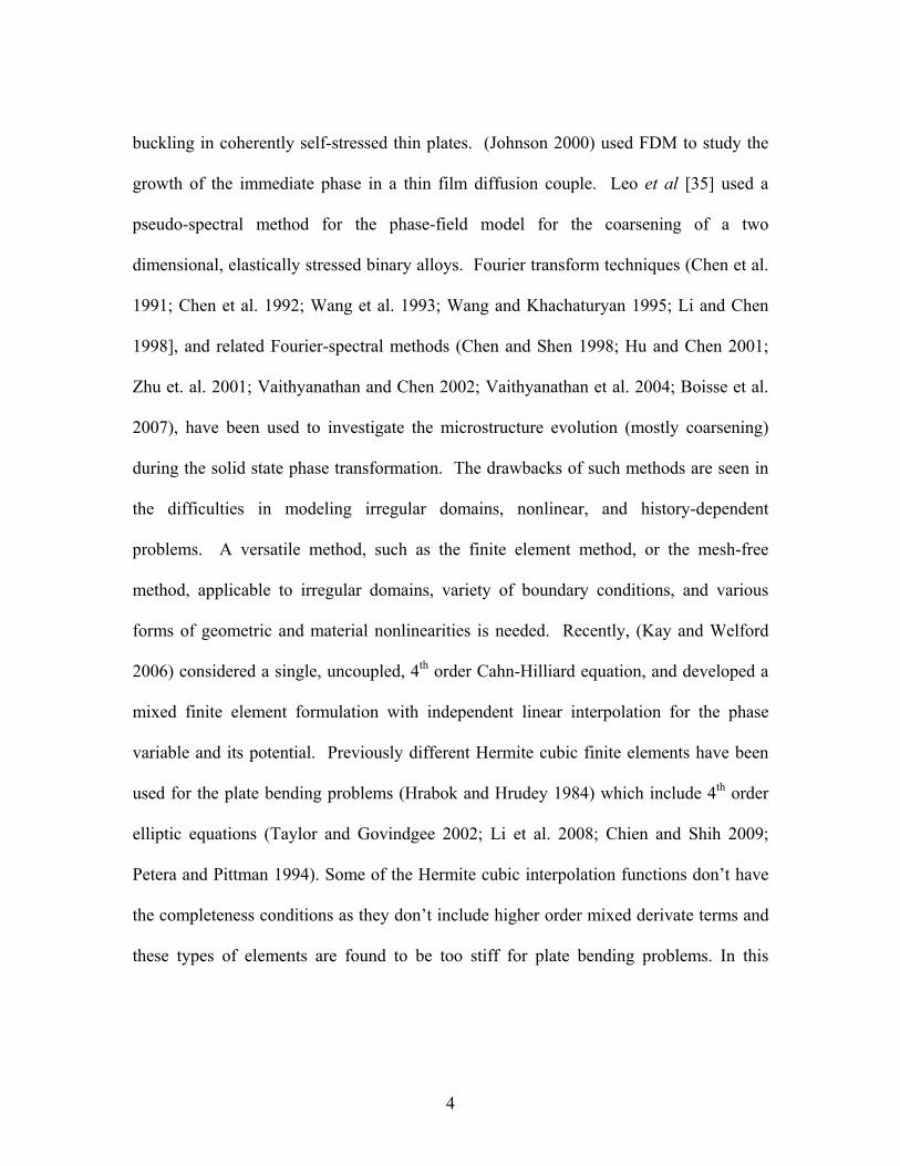
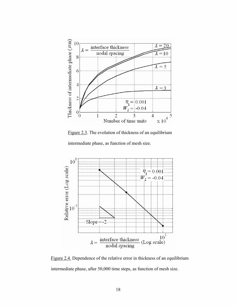
Figure 2.3. The evolution of thickness of an equilibrium intermediate phase, as

function of mesh size. ...........................................................................................18

Figure 2.4. Dependence of the relative error in thickness of an equilibrium

intermediate phase, after 50,000 time steps, as function of mesh size. ................18

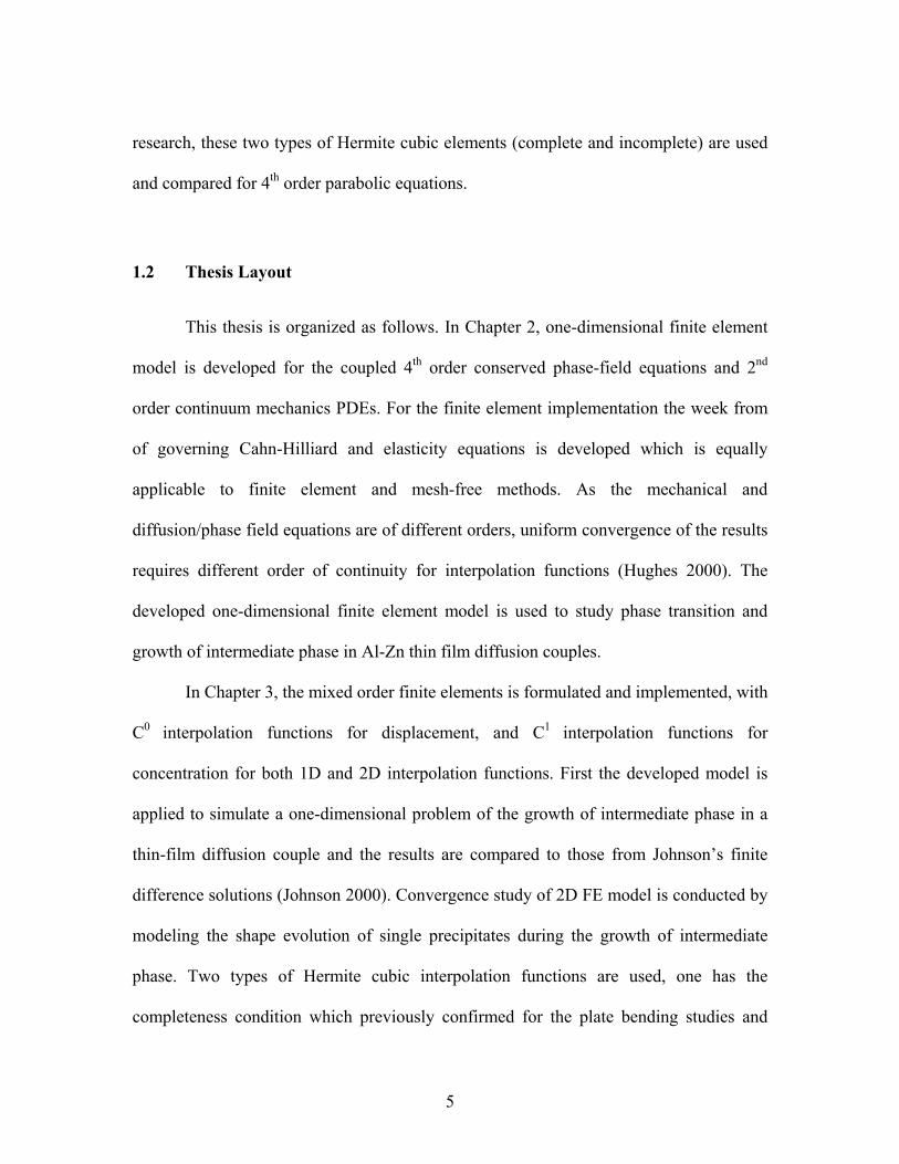
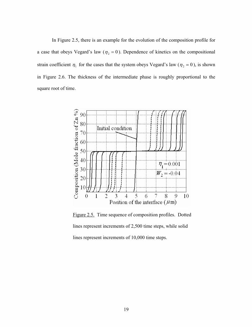
Figure 2.5. Time sequence of composition profiles. Dotted lines represent

increments of 2,500 time steps, while solid lines represent increments of

10,000 time steps. ..................................................................................................19

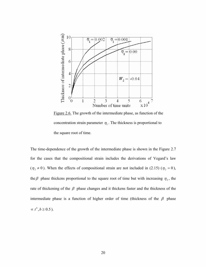
Figure 2.6. The growth of the intermediate phase, as function of the concentration

strain parameter 1η . The thickness is proportional to the square root of time. ....20

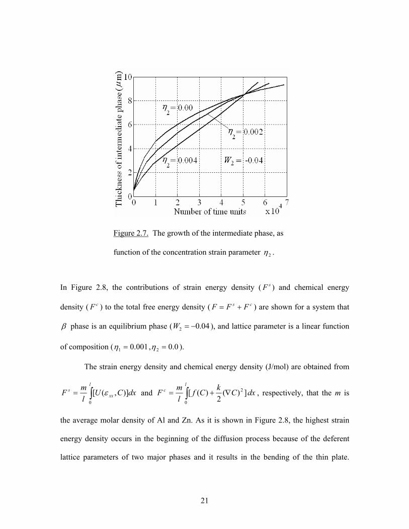
Figure 2.7. The growth of the intermediate phase, as function of the concentration

strain parameter 2η . ..............................................................................................21

Figure 2.8. The chemical, elastic and free energies of the thin-plate diffusion couple

when the intermediate phase is in equilibrium. ....................................................22

Figure 2.9. The evolution of thickness of a meta-stable intermediate phase, as

function of mesh size. ...........................................................................................24

Figure 2.10. Dependence of the relative error in thickness of a meta-stable

intermediate phase after 30,000 time steps, as function of mesh size. .................24

Figure 2.11. The growth of the meta-stable intermediate phase, as function of the

concentration strain parameter 1η ..........................................................................25

x

Figure 2.12. Time sequence of composition profiles for the case of arrested growth.

Dotted lines represent increments of 3,000 time steps, solid line represent

increments of 12,000 time units. The growth of the intermediate phase stops

after approximately 60,000 time steps. .................................................................25

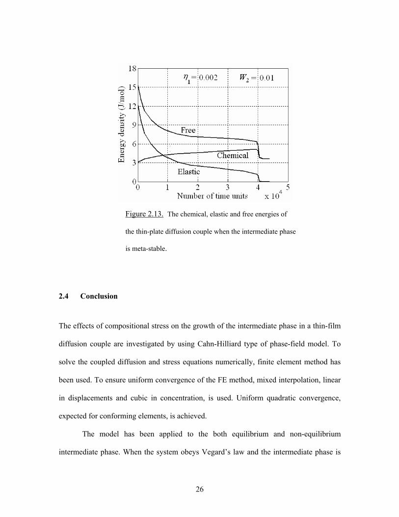
Figure 2.13. The chemical, elastic and free energies of the thin-plate diffusion couple

when the intermediate phase is meta-stable. .........................................................26

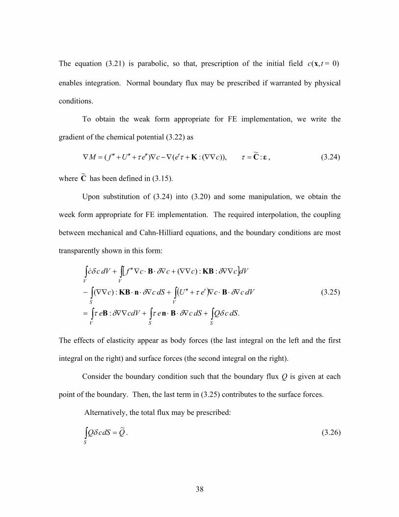
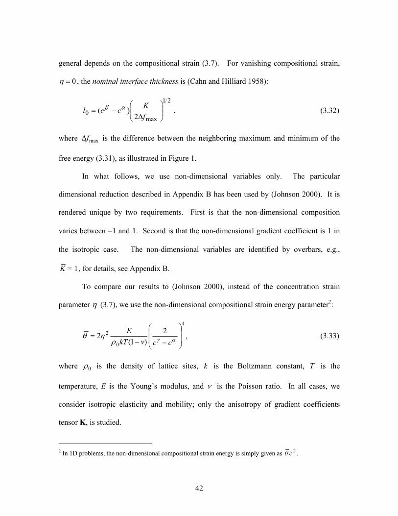
Figure 3.1. The non-dimensional triple-well free energy density, as function of scaled

concentration (scaling is given in Appendix B). Depending on the value of

2W , the intermediate phase is stable or metastable. ..............................................43

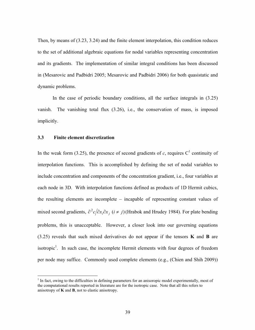
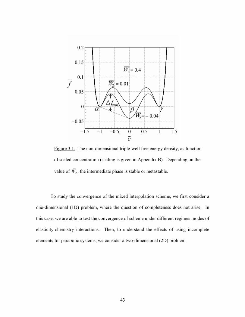
Figure 3.2. (a) Schematic representation of initial condition of the thin plate diffusion

couple. (b) β phase grows as the intermediate phase and the plate is free to

bend. ......................................................................................................................44

Figure 3.3. The non-dimensional thickness of the intermediate phase S , as function

of the non-dimensional time, t (Appendix B). Different mesh sizes are used

and the Johnson’s [8] finite difference results (FDM) are shown for

comparison. ...........................................................................................................46

Figure 3.4. Relative error (3.35) in the thickness of intermediate phase as function of

mesh parameter λ , at 316 10t = ´ . ......................................................................47

Figure 3.5. The thickness of meta-stable intermediate phase as function of time for

the different values of the compositional strain energy parameter θ .

Johnson’s [8] finite difference results (FDM) are shown for comparison. ...........48

Figure 3.6. (a) The growth of the stable-intermediate phase 0.05θ = . Color bar

shows the composition. (b) Mesh corresponding to the rectangle in (a) 0t = .

Complete elements are used, with 5=λ in the interface region. ........................50

Figure 3.7. For the geometry shown in Figure 3.6: thickness of the intermediate

phase as function of time for different mesh sizes and different types of

elements. ...............................................................................................................51

xi

Figure 3.8. Relative error in intermediate phase thickness as function of the mesh

parameter. The points correspond to the time 15,000 in Figure 3.7. ...................52

Figure 3.9. Phase transition is presented for the stable-intermediate phase,

2 0.04W = − , with a relatively high compositional strain energy parameter,

0.2θ = ( 5=λ , color bar shows the composition). .............................................54

Figure 3.10. The thickness of the intermediate phase is plotted as a function of time

for different values of concentration strain parameter θ . The initial

precipitate and cell geometry are shown in Figure 3.6. ........................................55

Figure 3.11. Shape evolution of an initially circular precipitate for a system with

stable intermediate phase ( 0.05θ = ), and anisotropy coefficient 25.0=µ .

Color bar shows composition. ...............................................................................57

Figure 3.12. The thickness of the stable intermediate phase (the longer length in

Figure 3.11) for 25.0=µ is plotted as a function of time for the different

values of µ . The precipitate initially has a circular shape with radius 20. ........58

Figure 4.1. The non-dimensional triple-well free energy density, f , as function of

scaled composition, c . ..........................................................................................73

Figure 4.2. Microstructural development in a single γ -layer embedded between two

α -layers. Initially 15=γd and 30=αd ; 07.0=η , color bar shows the

composition, the finite element mesh consists of 14182 triangular elements. ......75

Figure 4.3. Coarsening of γ -layers. Initially 25=γd and 15=αd ; 1.0=η , and

color bar shows the composition. The finite element mesh consists of 22248

triangular elements. ...............................................................................................77

Figure 4.4. Map of transformations for the systems with possibility of two phases (no-

intermediate phase) and 0=η . The non-dimensional interface thickness

calculated form (4.10) is 70 ≅l . All the results are from 710=t ........................77

xii

Figure 4.5. Map of transformations for the systems with possibility of two phases (no-

intermediate phase) and for 1.0=η . The non-dimensional interface thickness

calculated form (4.10) is 70 ≅l . All the results are from 710=t ........................78

Figure 4.6. Phase transition is presented for a system with stable-intermediate phase.

Initially 15=γd and 20=αd ; 2.0=η and color bar shows the composition.

The finite element mesh consists of 45108 triangular elements. ..........................79

Figure 4.7. Map of transformations for the systems with possibility of three phases

(stable-intermediate phase) and 0=η . The non-dimensional interface

thickness between β andγ phases calculated form (4.10) is 2.30 ≅l . All the

results are from 710=t .........................................................................................80

Figure 4.8. Map of transformations for the systems with possibility of three phases

(stable-intermediate phase) and 2.0=η . The non-dimensional interface

thickness between β andγ phases calculated form (4.10) is 2.30 ≅l . All the

results are from 710=t .........................................................................................81

Figure 4.9. Phase transition is presented for a case with meta-stable intermediate

phase. Initially 15=γd and 10=αd ; 2.0=η and color bar shows the

composition. The finite element mesh consists of 50200 triangular elements. ....82

Figure 4.10. Map of transformations for the systems with possibility of meta-stable

intermediate phase growth and 0=η . The non-dimensional interface

thickness between β andγ phases calculated form (4.10) is 8.20 ≅l . All the

results are from 810=t . ........................................................................................84

Figure 4.11. Map of transformations for the systems with possibility of meta-stable

intermediate phase growth and 2.0=η . The non-dimensional interface

thickness between β andγ phases calculated form (4.10) is 8.20 ≅l . All the

results are from 810=t . ........................................................................................84

1

CHAPTER ONE: Introduction

1.1 Microstructural Evolution and Phase Field Model Evolution of microstructures takes place in many fields including biology, hydro-

dynamics, chemical reactions, and phase transformations. During the processing of

materials, the microstructural evolution occurs to reduce the free energy of the system

and force the system to a low energy equilibrium condition. The size, shape, and spatial

arrangement of the local structural features in a microstructure play a critical role in

determining different properties of a material. These structural features usually have an

intermediate mesoscopic length scale in the range of nanometers to microns. Because of

the complexity and nonlinearity nature of microstructural evolution, numerical models

are often employed to investigate the behaviors of the microstructures under different

conditions. In the sharp-interface model (Caginalp and Xie 1993) which is the traditional

method for capturing the microstructural evolution, the regions separating the

compositional or structural fields are considered as mathematically sharp interfaces so

one or more variables (or their derivatives) are typically discontinuous across an

interface. The local velocity of interfacial regions is then determined as part of the

boundary conditions or calculated from the driving force for interface motion and the

interfacial mobility. This involves the explicit tracking of the interface positions. This

interface-tracking approach can be very successful in one-dimensional systems, but it

2

becomes impractical for complicated two and three-dimensional microstructures those

include intermediate phase growth, triple junctions, and etc.

Recently, the phase-field method has been found as a powerful computational tool

for modeling mesoscale microstructural evolution in materials. Phase-field model is

based on a diffuse-interface description developed more than a century ago by van der

Walls (Rowlinson 1979) and almost 50 years ago independently by (Cahn and Hilliard

1958). Phase-field models describe microstructure phenomena at the mesoscale and

include field variables corresponding to physical order parameters such as long-range

order parameters for order-disorder transformations and the composition fields for phase

separation. Phase-field models have been extensively applied to simulate solidification

and solid-state phase transformations (Ode et al. 2001; Chen and Wang 1996) and also

have been employed for modeling a number of other important materials processes

including grain growth and coarsening (Chen and Wang 1994; Steinbach et al. 1996;

Lusk 1999; Kobayashi et al. 2000), phase transformations in thin films (Li et al. 2001;

Seol et al. 2003; Atemev et al. 2008), crack propagation (Aranson et al. 2000; Karma et

al. 2001; Karma and Lobkovsky 2003; Spatschek et al. 2006; Song et al. 2007),

dislocation dynamics (Wang et al. 2001; Wang et al. 2003; Koslowski and Ortiz 2004),

and etc.

Phase-field models are characterized by the dependence of the free energy of a

non-uniform system on the phase field variable. Mathematically, the phase-field

formulation gives rise to two types of problems. The non-conserved phase-field variables,

such as solidification and melting problems (Fan et al. 2006; Provatas et al. 1998; Sabouri

3

et al. 2001), are often assumed to evolve according to the “first-order relaxation”,

whereby the rate of change of the phase variable is proportional to the variational

derivative of the free energy, mediated by the kinetic mobility. Such formulation leads to

a 2nd order, diffusion-type, evolution PDE for the phase field variable (Wang and

Khachaturyan 1997; Wen et al. 1999). However, if the phase-field variable is subject to a

conservation law, then the rate of the phase field variable is proportional to the

divergence of the flux, which, in turn, is proportional to the gradient of a potential. This

potential is equal to the variational derivative of the free energy. Examples include

diffusion-controlled solid state phase transformations (Cahn and Hilliard 1958; Cahn and

kobayashi 1995; Johnson 2000; Leo and Johnson 2001), and interfaces between

immiscible fluids (Jacqmin 19999; Anderson et al. 1998). Typically, the 4th order

evolution PDE is coupled to a 2nd order PDEs (stress, heat, etc.). For example, in solid

state phase transformations, the lattice continuity across the interfaces between

mismatched phases produces elastic strains (Khachaturyan 1983; Cahn and Larche 1982;

Larche and Cahn 1992; Khachaturyan et al. 1996), so that the 2nd order elasticity PDEs

are coupled to the phase field equation (Cahn and Hilliard 1958; Cahn and kobayashi

1995; Johnson 2000; Leo and Johnson 2001; Leo et al. 1998; Chen et al. 1991).

The problems in this class have been addressed in the past, with the numerical

tools tailored for specific problems. However, a general numerical method for solving

the coupled equations, applicable to variety of geometries and boundary conditions, has

remained a challenging problem. The finite difference method (FDM) was used by

(Cahn and Kobayashi 1995) for one-dimensional modeling of the rapid coarsening and

4

buckling in coherently self-stressed thin plates. (Johnson 2000) used FDM to study the

growth of the immediate phase in a thin film diffusion couple. Leo et al [35] used a

pseudo-spectral method for the phase-field model for the coarsening of a two

dimensional, elastically stressed binary alloys. Fourier transform techniques (Chen et al.

1991; Chen et al. 1992; Wang et al. 1993; Wang and Khachaturyan 1995; Li and Chen

1998], and related Fourier-spectral methods (Chen and Shen 1998; Hu and Chen 2001;

Zhu et. al. 2001; Vaithyanathan and Chen 2002; Vaithyanathan et al. 2004; Boisse et al.

2007), have been used to investigate the microstructure evolution (mostly coarsening)

during the solid state phase transformation. The drawbacks of such methods are seen in

the difficulties in modeling irregular domains, nonlinear, and history-dependent

problems. A versatile method, such as the finite element method, or the mesh-free

method, applicable to irregular domains, variety of boundary conditions, and various

forms of geometric and material nonlinearities is needed. Recently, (Kay and Welford

2006) considered a single, uncoupled, 4th order Cahn-Hilliard equation, and developed a

mixed finite element formulation with independent linear interpolation for the phase

variable and its potential. Previously different Hermite cubic finite elements have been

used for the plate bending problems (Hrabok and Hrudey 1984) which include 4th order

elliptic equations (Taylor and Govindgee 2002; Li et al. 2008; Chien and Shih 2009;

Petera and Pittman 1994). Some of the Hermite cubic interpolation functions don’t have

the completeness conditions as they don’t include higher order mixed derivate terms and

these types of elements are found to be too stiff for plate bending problems. In this

5

research, these two types of Hermite cubic elements (complete and incomplete) are used

and compared for 4th order parabolic equations.

1.2 Thesis Layout

This thesis is organized as follows. In Chapter 2, one-dimensional finite element

model is developed for the coupled 4th order conserved phase-field equations and 2nd

order continuum mechanics PDEs. For the finite element implementation the week from

of governing Cahn-Hilliard and elasticity equations is developed which is equally

applicable to finite element and mesh-free methods. As the mechanical and

diffusion/phase field equations are of different orders, uniform convergence of the results

requires different order of continuity for interpolation functions (Hughes 2000). The

developed one-dimensional finite element model is used to study phase transition and

growth of intermediate phase in Al-Zn thin film diffusion couples.

In Chapter 3, the mixed order finite elements is formulated and implemented, with

C0 interpolation functions for displacement, and C1 interpolation functions for

concentration for both 1D and 2D interpolation functions. First the developed model is

applied to simulate a one-dimensional problem of the growth of intermediate phase in a

thin-film diffusion couple and the results are compared to those from Johnson’s finite

difference solutions (Johnson 2000). Convergence study of 2D FE model is conducted by

modeling the shape evolution of single precipitates during the growth of intermediate

phase. Two types of Hermite cubic interpolation functions are used, one has the

completeness condition which previously confirmed for the plate bending studies and

6

another one doesn’t have the completeness condition which we want to examine if it

works for parabolic equations like Cahn-Hillirad equation and under what conditions.

In chapter 4, the 2D model is applied to study the stability of multilayer thin film

diffusion couples in solid state. Maps of transformations in multilayer systems are carried

out considering the effects of interface thickness between phases, thickness of layers, and

elastic strain on the stability of the multilayer systems.

7

CHAPTER TWO: Investigation of Phase Transformation in

Thin Film Using Finite Element Method

(Published in Solid State Phenomena, 2009, Volume 150, Pages 29-41)

Mohsen Asle Zaeem and Sinisa Dj. Mesarovic

School of Mechanical and Materials Engineering

Washington State University, Pullman, WA, 99164 USA

Abstract

Cahn-Hilliard type of phase field model coupled with elasticity is used to derive

governing equations for the stress-mediated diffusion and phase transformation in thin

films. To solve the resulting equations, a finite element (FE) model is presented. The

partial differential equations governing diffusion and mechanical equilibrium are of

different orders; Mixed-order finite elements, with C0 interpolation functions for

displacement, and C1 interpolation functions for concentration are implemented. To

validate this new numerical solver for such coupled problems, we test our

implementation on a 1D problem and demonstrate the validity of the approach.

Keywords: Phase transformation, solid state, thin film, phase field model, finite element (FE).

8

2.1 Introduction A sequential formation of the intermediate phase occurs in binary diffusion couples and

the intermediate phase nucleates and grows until one of the end phases is consumed.

Several researches have been done to find proper diffuse interface models for capturing

the evolution of microstructure formed during the diffusion between two major phases in

binary alloys (Cahn and Kobayashi 1995; Leo et al. 1998; Johnson 1997; Johnson 2000;

Hu and Chen 2001; Hinderliter and Johnson 2002; Ahmed 2007; Wang et al. 2007). Cahn

and Kobayashi (Cahn and Kobayashi 1995) showed that the coupling between stress and

diffusion can have a strong effect on the microstructural evolution. (Johnson 2000)

studied the growth of the intermediate phase in binary alloys. He showed that the

compositional strains can lead to bending of the mechanically unconstrained thin plates.

In this class of coupled problems, the question of a general, versatile numerical method

for solving the coupled equations, applicable to a variety of geometries and boundary

conditions, is the main issue. The finite difference method used by (Johnson 2000), and

the more common Fourier-spectral methods (Hu and Chen 2001), have own limitations.

The finite element method seems to be the most versatile tool for modeling this class of

problems, especially when coupled with visco-plasticity and large deformation, most

commonly modeled in a Lagrangean framework with the resulting nonlinearities.

In this paper we use a weak form of the Cahn-Hilliard type of phase-field model

(Cahn and Hilliard 1958) coupled with elasticity, to derive the governing FE equations.

The equations are derived for a binary system that can exist in three phases and the lattice

parameter assumed to be both linear and quadratic function of the composition. As the

9

mechanical and diffusion/phase field equations are of different orders, uniform

convergence of the results requires different order of continuity for interpolation

functions (Hughes 2000). We formulate and implement such mixed-order finite elements,

with C0 interpolation functions for displacement, and C1 interpolation functions for

concentration. To test our formulation and implementation we consider different cases

for the Al-Zn binary system. The results are in good agreement with Johnson’s finite

difference method results (Johnson 2000).

2.2 Formulation

2.2.1 Phase field model

A binary alloy with two components A and B is considered. The alloy forms three

different phases that are assumed to be isostructural. The α phase is rich in component A

and has initial composition α0C , and the γ phase is rich in component B and has initial

composition γ0C . The intermediate phase is denoted β and has about 50% of each

component. Average composition 0C is taken as the reference composition for the

analyses. The lattice parameter )(Ca is assumed to be a linear or quadratic function of

composition:

202010 )()(1)()( CCCCCaCa −+−+= ηη , (2.1)

10

The material parameters 1η and 2η are the measures of the compositional strain; 2η is a

measure of the derivation of Vegard’s law (Denton and Ashcroft 1991) ( 2η is 0 when the

system obeys Vegard’s law). The compositional strain has the form:

20201

0

0 )()()(

)()(CCCC

CaCaCa

e −+−=−

= ηη . (2.2)

The total free energy of a non-uniform system with volume V, bounded by surface S,

is given as:

∫∫∫ ⋅−+∇++=SSV

dSdSCdVCkCUCfF ut)(])(2

),()([ 2 γε , (2.3)

where the last term represents the loading potential, with surface tractions t and

displacement vector u. C is the mole fraction of component B, ),( CU ε is the strain

energy density, ε is the total strain tensor, k is the composition-independent gradient

energy coefficient (scalar for a cubic system (Cahn and Hilliard 1958)), )(Cγ is the

surface free energy density. The Helmholtz free energy density of a uniform unstressed

system at concentration C, )(Cf , is assumed to be a three well potential (Johnson 2000)

as illustrated in Figure 2.1:

222

2221

0

)()()()()()( γαγβα

ρCCCCWCCCCCCW

KTCf

−−+−−−= , (2.4)

where 1W and 2W are the energy coefficients, 0ρ is density of the lattice sites, K is

Boltzmann’s constant, and T is the temperature. αC , βC and γC are the mole fractions

of component B at which the Helmholtz free energy of the uniform unstressed system has

minima. The parameters in (2.4) are chosen so that 2/)( γαβ CCC += . Depending on

11

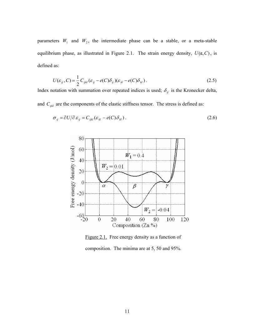
parameters 1W and 2W , the intermediate phase can be a stable, or a meta-stable

equilibrium phase, as illustrated in Figure 2.1. The strain energy density, ),( CU ε , is

defined as:

))()()((21),( klklijijijklij CeCeCCU δεδεε −−= . (2.5)

Index notation with summation over repeated indices is used; ijδ is the Kronecker delta,

and ijklC are the components of the elastic stiffness tensor. The stress is defined as:

))(( klklijklijij CeCU δεεσ −=∂∂= . (2.6)

Figure 2.1. Free energy density as a function of

composition. The minima are at 5, 50 and 95%.

12

2.2.2 Equilibrium Conditions

Considering zero flux on the boundaries, the conservation of mass requires:

∫ −V

dVCC )( 0 . (2.7)

The equilibrium problem is one of constrained minimization of free energy (2.3),

under constraint (2.7). Upon introducing the Lagrange multiplier, 0M , we seek to

minimize the functional:

∫ −−=V

dVCCMFF )( 00 . (2.8)

For isothermal chemical and mechanical equilibria, we require that variational

derivatives of (2.8) with respect to C and u, vanish: 0=FCδ , and 0=Fuδ . The

chemical equilibrium requires

[ ] [ ] 0'''' 02 =∇⋅−++−∇−+= ∫∫

VVC dSCCkUdVCMCkUfF δγδδ n , (2.9)

for arbitrary variation Cδ . The primes denote partial derivatives with respect to

concentration, e.g., Cff ∂∂=' . This implies:

==∇−+ 02'' MCkUf constant, in V, (2.10)

0' =∇⋅+ Cknγ , on S. (2.11)

The mechanical equilibrium requires:

0,,, =−−= ∫∫∫S

jjV

ijijkkV

ijklijkl dSutdVueCdVuuCF δδδδu . (2.12)

13

2.2.3 Diffusion

Local conservation of concentration, C, implies that its local value changes according to

the divergence of its flux J:

J⋅−∇=C&0ρ . (2.13)

In a multi-component solid under stress, the chemical potential, which is constant

at equilibrium (2.10) is determined from the variational derivative of free energy respect

to composition (Larche and Cahn 1978):

)''( 2CkUfCFM ∇−+== δδ . (2.14)

The flux of C is proportional to gradient of the chemical potential, M:

MB∇−= 0ρJ , (2.15)

where B is the mobility, assumed to be a function of temperature only. The equation for

the time evolution of composition becomes:

)''( 22 CkUfBC ∇−+∇=& . (2.16)

Since the chemical potential (2.14) depends on second order derivatives of composition,

(2.16) is fourth order PDE in composition. For finite element implementation, we start

from (2.13) and follow the usual procedure to derive the week form:

00 =⋅+∇⋅− ∫∫∫ dSCdVCdVCCSVV

δδδρ JnJ& . (2.17)

Since there is no flux on the boundaries, the third integral in (2.17) vanishes. Then, using

(2.15) and (2.16):

.0,],,',)''''[( =−∂∂

+++ ∫∫ dVCkCUCUfBdVCC iV

kkiipqpq

iV

δεε

δ& (2.18)

14

2.2.4 Finite element method

The coupled mechanical equation (2.12) and phase field /diffusion equation (2.18) are

solved numerically for a thin film diffusion couple, schematically shown in Figure 2.2,

using the finite element method. The partial differential equations governing diffusion

and mechanical equilibrium are of different orders so mixed-order finite element

implementation is needed. Two-node linear elements with regular C0 interpolation

functions are used to generate the mesh along the plate-thickness for the mechanical

equation (2.12). As the diffusion/phase field equation is 4th order in concentration, the

standard convergence theorems require C1 continuity (like beam elements) (Hughes

2000), so two-node nonlinear elements with Hermite cubic polynomials are used to

discretize the domain for concentration, (2.18). Different mesh sizes are examined along

the plate thickness of the thin-film diffusion couple to find the proper mesh size.

The resulting FE equations consist of two sets of equations: a set of algebraic

equilibrium equations for displacement, and a set of 1st ODE for concentration degrees of

freedom. The FE equations resulting from equation (2.12) can be written in matrix form

as:

][ FuΚ = , (2.19)

u is the vector of nodal displacements, ][Κ is the stiffness matrix, and F is the force

vector that depends on compositional strain. The FE equations resulting from equation

(2.18) can be written in matrix form as:

][][ hΓdΓM =+& , (2.20)

15

Γ is the vector of nodal concentrations and its gradients. The order of the governing

equations dictates that the interpolation includes both nodal concentration, and its

gradients. Note that both matrix ][d and vector h depend on mechanical equations

(stress).

A special time integration scheme was developed consisting of implicit time-

stepping and equilibrium iterations in each time step. At time t, the matrix [d] and vector

h are known. We first estimate Γ at tt ∆+ by applying the Euler time

integration scheme to (2.20). Then, we iterate to satisfy equilibrium (2.19) at tt ∆+ ,

with corrections to (2.20), to obtain the values of both Γ and u at tt ∆+ .

Figure 2.2. (a) Schematic representation of initial β phase grows as

the intermediate phase and the plate is free to bend. (b) condition of

the thin plate diffusion couple.

16

2.3 Results and discussions

Components A and B in the thin-film diffusion couple are assumed to be Aluminum and

Zinc, respectively, and the initial compositions (mole fraction of Zn) for the α and γ

phases are assumed to be 05.00 =αC and 95.00 =γC , respectively. Initial composition

profile for the interface is assumed to be 50% of α and 50% of γ . The gradient energy

coefficient, k, at 300 Co , is assumed to be 11102.1 −× (J/m) according to the pair-wise

interaction between the atoms (Wang et al. 2007; Cahn and Hilliard 1958). All the other

parameters used for Al-Zn system are at the temperature of 300 Co (Lass et al. 2006;

Dinsdale 1991, Cui et al. 2006) [14-16]. The results are divided in two groups, first the

results for the systems that the intermediate phase, β , is an equilibrium phase

( 04.02 −=W ). The second case includes systems in which the intermediate phase is a

meta-stable phase ( 01.02 =W ). We have determined that the optimal time step is 0.02

seconds and have used it in all computations.

2.3.1 An equilibrium intermediate phase ( 04.02 −=W )

The characteristic length of the problem is the thickness of the interface (Cahn and

Hilliard 1958):

21

max22

/)(

⎟⎟⎠

⎞⎜⎜⎝

⎛∆

∆=−

=fkC

dxdCCCl

γα, (2.21)

17

where maxf∆ is the maximum free energy difference in Figure 2.1,

45.0~αγ CCCCC cc −=−=∆ and two phases attain same critical composition, cC ,

at the critical temperature. For 04.02 −=W , the interface thickness is ml µ47.0~ . We

first study the convergence of the FE method for 04.02 −=W , 001.01 =η and mµ10

plate thickness. The results are shown in Figures 2.3 and 2.4. The computational time

increases drastically with the mesh density, so that finding the optimal mesh size is of

practical importance. For element size h, we define the non-dimensional mesh

parameter:

hl /=λ . (2.22)

From the results in Figure 2.3, the optimal mesh size seems to be about 1/10 of the

interface width (interface of α - β and β -γ , or 1/5 of the α - β interface), i.e., 10=λ .

Since the exact solution is unknown, we define the relative error in quantity S )(λ , the

thickness of the interface as a function of non-dimensional mesh parameter λ , with

respect to the most accurate results which is from 20=λ :

)20()20()()(

SSSRS

−=

λλ . (2.23)

From Figure 2.4 it is evident that the relative error is approximately quadratic in mesh

size. Thus, the application of mixed-order interpolation (linear and Hermite cubic) results

in uniform convergence. Using the optimal mesh 10=λ , we study the evolution of the

intermediate phase.

18

Figure 2.3. The evolution of thickness of an equilibrium

intermediate phase, as function of mesh size.

Figure 2.4. Dependence of the relative error in thickness of an equilibrium

intermediate phase, after 50,000 time steps, as function of mesh size.

19

In Figure 2.5, there is an example for the evolution of the composition profile for

a case that obeys Vegard’s law ( 02 =η ). Dependence of kinetics on the compositional

strain coefficient 1η for the cases that the system obeys Vegard’s law ( 02 =η ), is shown

in Figure 2.6. The thickness of the intermediate phase is roughly proportional to the

square root of time.

Figure 2.5. Time sequence of composition profiles. Dotted

lines represent increments of 2,500 time steps, while solid

lines represent increments of 10,000 time steps.

20

The time-dependence of the growth of the intermediate phase is shown in the Figure 2.7

for the cases that the compositional strain includes the derivations of Vegard’s law

( 02 ≠η ). When the effects of compositional strain are not included in (2.15) ( 02 =η ),

the β phase thickens proportional to the square root of time but with increasing 2η , the

rate of thickening of the β phase changes and it thickens faster and the thickness of the

intermediate phase is a function of higher order of time (thickness of the β phase

5.0, ≥∝ bt b ).

Figure 2.6. The growth of the intermediate phase, as function of the

concentration strain parameter 1η . The thickness is proportional to

the square root of time.

21

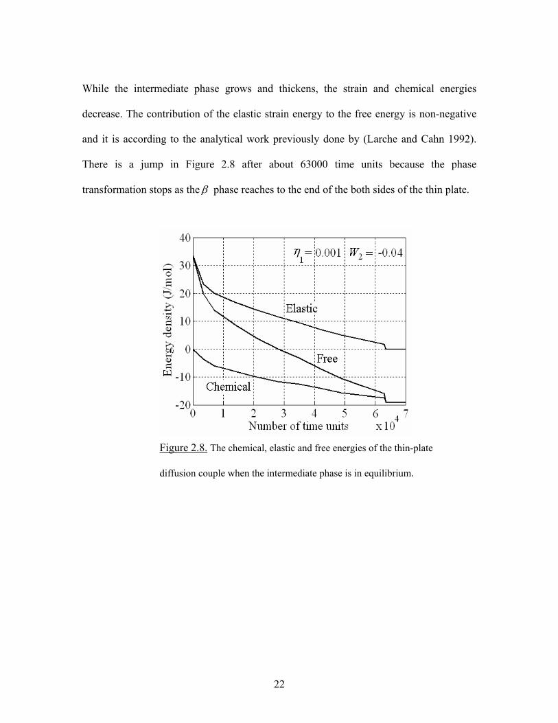
In Figure 2.8, the contributions of strain energy density ( sF ) and chemical energy

density ( cF ) to the total free energy density ( cs FFF += ) are shown for a system that

β phase is an equilibrium phase ( 04.02 −=W ), and lattice parameter is a linear function

of composition ( 001.01 =η , 0.02 =η ).

The strain energy density and chemical energy density (J/mol) are obtained from

∫=l

xxs dxCU

lmF

0

)],([ ε and ∫ ∇+=l

c dxCkCflmF

0

2 ])(2

)([ , respectively, that the m is

the average molar density of Al and Zn. As it is shown in Figure 2.8, the highest strain

energy density occurs in the beginning of the diffusion process because of the deferent

lattice parameters of two major phases and it results in the bending of the thin plate.

Figure 2.7. The growth of the intermediate phase, as

function of the concentration strain parameter 2η .

22

While the intermediate phase grows and thickens, the strain and chemical energies

decrease. The contribution of the elastic strain energy to the free energy is non-negative

and it is according to the analytical work previously done by (Larche and Cahn 1992).

There is a jump in Figure 2.8 after about 63000 time units because the phase

transformation stops as the β phase reaches to the end of the both sides of the thin plate.

Figure 2.8. The chemical, elastic and free energies of the thin-plate

diffusion couple when the intermediate phase is in equilibrium.

23

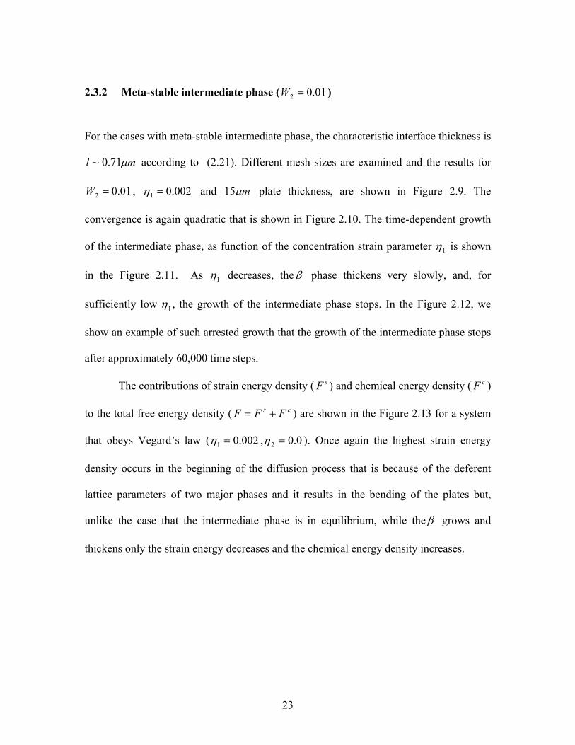
2.3.2 Meta-stable intermediate phase ( 01.02 =W ) For the cases with meta-stable intermediate phase, the characteristic interface thickness is

ml µ71.0~ according to (2.21). Different mesh sizes are examined and the results for

01.02 =W , 002.01 =η and mµ15 plate thickness, are shown in Figure 2.9. The

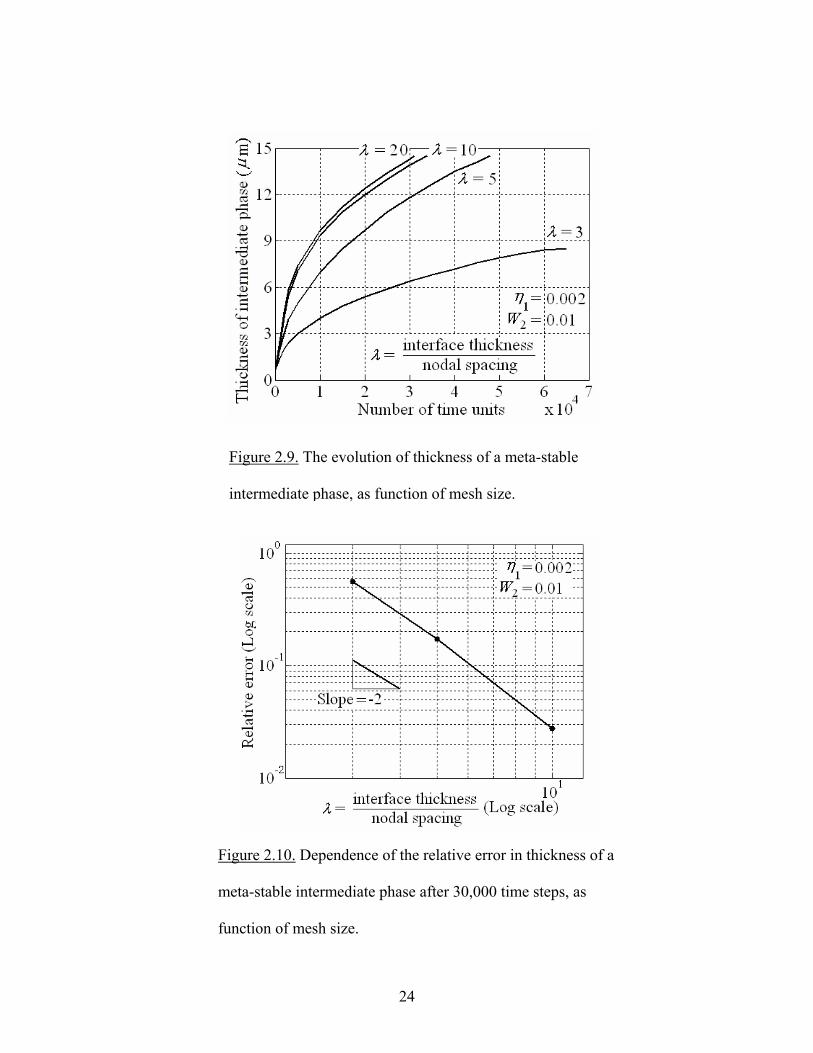
convergence is again quadratic that is shown in Figure 2.10. The time-dependent growth

of the intermediate phase, as function of the concentration strain parameter 1η is shown

in the Figure 2.11. As 1η decreases, the β phase thickens very slowly, and, for

sufficiently low 1η , the growth of the intermediate phase stops. In the Figure 2.12, we

show an example of such arrested growth that the growth of the intermediate phase stops

after approximately 60,000 time steps.

The contributions of strain energy density ( sF ) and chemical energy density ( cF )

to the total free energy density ( cs FFF += ) are shown in the Figure 2.13 for a system

that obeys Vegard’s law ( 002.01 =η , 0.02 =η ). Once again the highest strain energy

density occurs in the beginning of the diffusion process that is because of the deferent

lattice parameters of two major phases and it results in the bending of the plates but,

unlike the case that the intermediate phase is in equilibrium, while the β grows and

thickens only the strain energy decreases and the chemical energy density increases.

24

Figure 2.9. The evolution of thickness of a meta-stable

intermediate phase, as function of mesh size.

Figure 2.10. Dependence of the relative error in thickness of a

meta-stable intermediate phase after 30,000 time steps, as

function of mesh size.

25

Figure 2.11. The growth of the meta-stable intermediate

phase, as function of the concentration strain parameter 1η .

Figure 2.12. Time sequence of composition profiles for the case of arrested

growth. Dotted lines represent increments of 3,000 time steps, solid line represent

increments of 12,000 time units. The growth of the intermediate phase stops after

approximately 60,000 time steps.

26

2.4 Conclusion

The effects of compositional stress on the growth of the intermediate phase in a thin-film

diffusion couple are investigated by using Cahn-Hilliard type of phase-field model. To

solve the coupled diffusion and stress equations numerically, finite element method has

been used. To ensure uniform convergence of the FE method, mixed interpolation, linear

in displacements and cubic in concentration, is used. Uniform quadratic convergence,

expected for conforming elements, is achieved.

The model has been applied to the both equilibrium and non-equilibrium

intermediate phase. When the system obeys Vegard’s law and the intermediate phase is

Figure 2.13. The chemical, elastic and free energies of

the thin-plate diffusion couple when the intermediate phase

is meta-stable.

27

an equilibrium phase, for different values of 1η , the intermediate phase thickens

approximately proportional to the square root of time; and when the intermediate phase is

a meta-stable phase, with decreasing 1η , the growth of intermediate phase reduces, even

in very small 1η the growth stops after a very short time steps. When the system includes

the derivation of Vegard’s law and the intermediate phase is an equilibrium phase, as 1η

increases, the thickness of the β phase gets proportional to the higher order of the time

( β thickness 5.0, ≥∝ bt b ). For the case that the intermediate phase is meta-stable, as 1η

decreases, the β phase thickens very slowly and for very low 1η , the growth of the

intermediate phase stops after few steps.

28

CHAPTER THREE: Finite element method for conserved phase fields:

Stress-mediated diffusional phase transformation

(Submitted to Journal of Computational Physics, 2010)

Mohsen Asle Zaeem and Sinisa Dj. Mesarovic

School of Mechanical and Materials Engineering, Washington State University, Pullman,

WA, 99164 USA

Abstract

The phase-field models with conserved phase-field variables result in a 4th order

evolution partial differential equations (PDE). When coupled with the usual 2nd order

thermo-mechanics equations, such problems require special treatment. In the past, the

finite element method (FEM) has been successfully applied to non-conserved phase

fields, governed by 2nd order PDE. For higher order equations, the uniform convergence

of the standard Galerkin FEM requires that the interpolation functions belong to a higher

continuity class.

We consider the Cahn-Hilliard phase-field model for diffusion-controlled solid

state phase transformation in binary alloys, coupled with elasticity of the solid phases. A

Galerkin finite element formulation is developed, with mixed-order interpolation: C0

interpolation functions for displacements, and C1 interpolation functions for the phase-

field variable.

29

To demonstrate uniform convergence of the mixed interpolation scheme, we first

study a one-dimensional problem – nucleation and growth of the intermediate phase in a

thin-film diffusion couple with elasticity effects. Then, we study the effects of

completeness of C1 interpolation on parabolic problems in two space dimensions by

considering the growth of the intermediate phase in solid state binary systems.

Uniform quadratic convergence, expected for conforming elements, is achieved

for both one- and two-dimensional systems.

Keywords: phase-field model, Galerkin finite element method, binary alloys,

convergence

3.1 Introduction

A broad spectrum of moving boundary problems can be successfully handled with the

diffuse-interface or phase-field models. Such models are constructed by assuming that

the free energy of a non-uniform system F, depends on – among other variables – the

phase-field variable φ , and its gradient φ∇ . In the volume V:

∫ ∇=V

dVgF ),( φφ . (3.1)

Mathematically, the phase-field formulation gives rise to two types of problems.

The non-conserved phase-field variables, such of those in solidification and

melting problems (Fan et al. 2006; Provatas et al. 1998; Sabouri et al. 2001), are often

30

assumed to evolve according to the “first-order relaxation”, whereby the rate of change of

the phase variable, φ& , is proportional to the variational derivative of the free energy,

mediated by the kinetic mobility B:

δφδφ FB−=& .

Such formulation leads to a 2nd order, diffusion-type partial differential equation (PDE)

for φ (Wang et al. 1997; Wen et al. 1999). However, if the phase-field variable is

subject to a conservation law, e.g.,

0=∫V dVdtd φ , (3.2)

then the rate φ& is proportional to the divergence of the flux, which in turn, is proportional

to the gradient of a potential. This potential is equal to the variational derivative of the

free energy:

)]([ δφδφ FB∇−⋅−∇=& . (3.3)

Examples include diffusion-controlled solid-state phase transformations (Cahn and

Hilliard 1958, Cahn and Kobayashi 1995; Johnson 2000; Leo and Johnson 2001), and

interfaces between immiscible fluids (Jacqmin 1999; Anderson et al. 1998). Typically,

the 4th order evolution PDE (3.3) is coupled to a 2nd order PDEs (stress, heat, etc.). For

example, in solid state phase transformations, the lattice continuity across the interfaces

between mismatched phases produces elastic strains (Khachaturyan 1983; Cahn and

Larche 1982; Larche and Cahn 1992; Khachaturyan et al. 1996), so that the 2nd order

elasticity PDEs are coupled to the phase field equation (3.3) (Cahn and Kobayashi 1995;

Johnson 2000; Leo and Johnson 2001; Leo et al. 1998; Chen et al. 1991; Chen et al.

1992; Wang et al. 1993; Wang and Khachaturyan 1995, Li and Chen 1998).

31

The problems in this class have been addressed in the past, with the numerical

tools tailored for specific problems. However, a general numerical method for solving

the coupled equations, applicable to variety of geometries and boundary conditions, has

remained a challenging problem. The finite difference method (FDM) was used by

(Cahn and Kobayashi 1995) for one-dimensional modeling of the rapid coarsening and

buckling in coherently self-stressed thin plates. (Johnson 2000) used FDM to study the

growth of the intermediate phase in a thin film diffusion couple. (Leo et al. 1998) used a

pseudo-spectral method for the phase-field model for the coarsening of a two

dimensional, elastically stressed binary alloys. Fourier transform techniques (Chen et al.

1991; Chen et al. 1992; Wang et al. 1993; Wang et al. 1995; Li and Chen 1998), and

related Fourier-spectral methods (Chen and Shen 1998; Hu and Chen 2001; Zhu et al.

2001; Vaithyanathan and Chen 2002; Vaithyanathan et al. 2004; Boisse et al. 2007), have

been used to investigate the microstructure evolution (mostly coarsening) resulting from

solid-state phase transformations. The drawbacks of such methods are seen in the

difficulties in modeling irregular domains, nonlinear and history-dependent problems. A

versatile method is needed, such as the finite element method (FEM), or the mesh-free

method, which is applicable to irregular domains, variety of boundary conditions, and

various forms of geometric and material nonlinearities.

The key issue in formulating the finite element method for 4th order problem is

the order of interpolation. To ensure convergence in the classical continuous Galerkin

method, C1 continuity is required (Hughes 2000). In dimensions higher than one,

standard Hermit cubics are incomplete. The elements used to solve the 4th order elliptic

32

plate bending problems are too stiff (Hrabok and Hrudey 1984; Taylor and Govindgee

2002; Li et al. 2008; Chien et al. 2009; Petera and Pittman 1994). Alternatives include:

(i) augmentation of the interpolation functions to insure completeness (Hrabok and

Hrudey 1984; Li et al. 2008; Chien et al. 2009), (ii) mixed, discontinuous formulation

(Engel 2002), and, (iii) the continuous-discontinuous formulation (Engel 2002). The

advantages and disadvantages are well understood for elliptic problems (Engel 2002).

Parabolic phase-field problems have received little attention. Only the mixed,

discontinuous Galerkin formulation has been applied to a single, uncoupled, 4th order

Cahn-Hilliard equation (Kay and Welford 2006).

In this paper we present the finite element formulation for coupled conserved

phase-field 4th order equations, and 2nd order continuum mechanics PDEs. We opt for the

classic continuous Galerkin formulation.

The weak form of governing Cahn-Hilliard and elasticity equations, developed in

Section 3.2, is equally applicable to finite element and mesh-free methods. As the

mechanical and diffusion/phase field equations are of different orders, uniform

convergence of the results requires different order of continuity for interpolation

functions. In Section 3.3, we formulate and implement such mixed-order finite elements,

with C0 interpolation functions for displacement, and C1 interpolation functions for

concentration. The computational results are presented in Section 3.4. We first

benchmark our code by comparing the results to Johnson’s (Johnson 2000) finite

difference solutions of one-dimensional problem of the growth of intermediate phase in

33

binary alloys (Asle Zaeem and Mesarovic 2009). Then, we consider two-dimensional

nucleation and growth of intermediate phase in binary alloys.

3.2 Phase field formulation, the weak form

A binary alloy, with components A and B, forms three phases, characterized by the molar

concentration c of the component A. The phases correspond to the minima of the stress-

free Helmholtz free energy density of a uniform system )(cf . The total free energy, F,

of a non-homogeneous system with volume V, bounded by surface S, is constructed as:

∫∫∫ ⋅−+⎥⎦⎤

⎢⎣⎡ ∇⋅⋅∇++=

SSVdSdScdVcccUcfcF utKεu )()()(

21),()(),( γ , (3.4)

The concentration ( )c x is now a scalar field over the domain. γ is the surface energy of

the outer surface S of the domain, and ε is the total strain tensor:

)(21 uuε ∇+∇= . (3.5)

),( cU ε is the strain energy density:

),(::)(21 IεCIε eeU −−= (3.6)

with the purely volumetric compositional strain e and C as the elastic coefficient tensor.

The simplest model follows the linear Vegard’s law (Denton and Ashcroft 1991):

0( )e c cη= - . (3.7)

34

The reference composition 0c is taken to be the average of composition over the domain.

In (3.4), the surface energy of the outer boundary S is neglected, and the last term is the

mechanical loading potential, with the surface traction t, and the displacement vector u.

The last term under the volume integral in (3.4) represents the interface energy density

between the phases. To ensure positive interface energy, the gradient energy coefficient

tensor, K, is assumed symmetric and positive definite. For an isotropic system it

simplifies to a scalar: IK K= , where I is the unit tensor.

With the strain energy (6), the stress is defined as:

)(: IεCεσ eU −=∂∂= . (3.8)

3.2.1 Equilibrium

When the total flux on the boundaries vanishes, the conservation of mass requires:

0)( 0 =−∫V

dVcc . (3.9)

The equilibrium problem is one of constrained minimization of free energy (3.4),

under constraint (3.9). Upon introducing the Lagrange multiplier, 0M , we seek to

minimize the functional:

∫ −−=V

dVccMFF )( 00 . (3.10)

35

For isothermal chemical and mechanical equilibria, the variational derivatives of

(3.10) with respect to c and u must vanish: 0~ =Fcδ , and, 0~ =Fuδ . Imposing this

condition for arbitrary variation cδ , we obtain the chemical equilibrium:

∫ ∫ =∇⋅⋅+′+−∇∇−′+′V S

dSccdVcMcUf 0)()(: 0 δγδ KnK , (3.11)

where primes indicate partial derivatives with respect to c, e.g., cUU ∂∂=′ , and n is the

unit outer normal to S. From (3.11), we extract the governing partial differential equation

and natural boundary conditions for chemical equilibrium:

0)(: McUf =∇∇−′+′ K in V, (3.12)

0)( =∇⋅⋅+′ cKnγ on S. (3.13)

The governing 2nd order PDE for the equilibrium concentration (3.12) is elliptic, owing to

the positive definiteness of K. The Lagrange multiplier 0M is the chemical potential,

uniform at equilibrium. For isotropic case, (3.13) specifies the vanishing normal gradient

at the boundary. For the sake of simplicity, we consider only the case 0=′γ .

Owing to the indeterminacy of 0M , the boundary condition (3.13) is insufficient

for uniqueness, so that the conservation of mass (3.9) must be enforced explicitly. On the

physical side, the argument is obvious; all three phases are equilibrium phases, but at

different concentration.

For arbitrary variation uδ , (3.10) is minimized if:

∫∫ =⋅−∇SV

dSdV 0)(: utuσ δδ . (3.14)

The differential equations governing mechanical equilibrium have the form:

36

ICCCuC :~,~)(: =∇⋅=∇⋅∇ e in V. (3.15)

The mathematical structure of boundary conditions is standard; at each point of the

boundary three of the six scalar components of traction tσn =⋅ and displacement u are

prescribed, but not the same components at one point.

For the purpose of finite element formulation, we write the weak form of

mechanical equations as:

∫ ∫∫ ⋅+∇=∇∇V SV

dSdVedV .)(:~)(::)( utuCuCu δδδ (3.16)

Diffusion-controlled phase transformations take place at the time scales much

longer than those required for wave propagation and attenuation in solids. Therefore, the

mechanical equilibrium will be assumed throughout the process, so that the weak form

(3.16) will be coupled to the weak form of the Cahn-Hilliard evolution equations (3.25).

The first term on the right hand side, effectively acting as a body force, introduces the

effects of concentration on the strains.

3.2.2 Diffusion

In the non-equilibrium case, local conservation of concentration implies that its local

value changes according to the divergence of its flux q:

q⋅−∇=c&0ρ . (3.17)

where 0ρ is the density of lattice sites. The flux is proportional to the gradient of

chemical potential, )(xM :

37

M∇⋅−= Bq 0ρ , (3.18)

where B is the symmetric, positive definite mobility tensor. It reduces to IB B= for

isotropic systems.

To simplify derivation, we will assume that mobility is uniform throughout the

domain. The weak form of (3.18) can be written as:

∫∫ =−∇⋅−SV

cdSQdVccc 0][ δδδ q& , (3.19)

where qn ⋅−=Q0ρ is the normal inward flux to the boundary. After some manipulation:

∫∫ =∇⋅⋅+−+∇⋅⋅∇−SV

cdSMQcdVMc 0)()]([ δδ BnB& . (3.20)

From (3.20), we extract the governing differential equation:

0)( =∇⋅⋅∇− Mc B& , in V. (3.21)

The chemical potential is the variational derivative of the free energy (3.11, 3.12) and is a

function of strain, concentration, and its second gradients: ),,( ccM ∇∇ε (Larche and

Cahn 1978).

)(: cUfM ∇∇−′−′= K , (3.22)

so that (3.21) is 4th order PDE in composition.

The natural boundary condition, arising from (3.20), provides the normal flux at

the boundary:

MQ ∇⋅⋅= Bn , on S. (3.23)

38

The equation (3.21) is parabolic, so that, prescription of the initial field ( , 0)c tx =

enables integration. Normal boundary flux may be prescribed if warranted by physical

conditions.

To obtain the weak form appropriate for FE implementation, we write the

gradient of the chemical potential (3.22) as

εCK :~)),(:()( =∇∇+′∇−∇′′+′′+′′=∇ τττ ceceUfM , (3.24)

where C~ has been defined in (3.15).

Upon substitution of (3.24) into (3.20) and some manipulation, we obtain the

week form appropriate for FE implementation. The required interpolation, the coupling

between mechanical and Cahn-Hilliard equations, and the boundary conditions are most

transparently shown in this form:

[ ]

( )

.:

:)(

::)(

dScQdScecdVe

dVcceUdScc

dVccccfdVcc

SV S

VS

VV

∫∫ ∫

∫∫

∫∫

+∇⋅⋅+∇∇=

∇⋅⋅∇′+′′+∇⋅⋅∇∇−

∇∇∇∇+∇⋅⋅∇′′+

δδτδτ

δτδ

δδδ

BnB

BnKB

KBB&

(3.25)

The effects of elasticity appear as body forces (the last integral on the left and the first

integral on the right) and surface forces (the second integral on the right).

Consider the boundary condition such that the boundary flux Q is given at each

point of the boundary. Then, the last term in (3.25) contributes to the surface forces.

Alternatively, the total flux may be prescribed:

QdScQS

~=∫ δ . (3.26)

39

Then, by means of (3.23, 3.24) and the finite element interpolation, this condition reduces

to the set of additional algebraic equations for nodal variables representing concentration

and its gradients. The implementation of similar integral conditions has been discussed

in (Mesarovic and Padbidri 2005; Mesarovic and Padbidri 2006) for both quasistatic and

dynamic problems.

In the case of periodic boundary conditions, all the surface integrals in (3.25)

vanish. The vanishing total flux (3.26), i.e., the conservation of mass, is imposed

implicitly.

3.3 Finite element discretization

In the weak form (3.25), the presence of second gradients of c, requires C1 continuity of

interpolation functions. This is accomplished by defining the set of nodal variables to

include concentration and components of the concentration gradient, i.e., four variables at

each node in 3D. With interpolation functions defined as products of 1D Hermit cubics,

the resulting elements are incomplete – incapable of representing constant values of

mixed second gradients, )(2 jixxc ji ≠∂∂∂ (Hrabok and Hrudey 1984). For plate bending

problems, this is unacceptable. However, a closer look into our governing equations

(3.25) reveals that such mixed derivatives do not appear if the tensors K and B are

isotropic1. In such case, the incomplete Hermit elements with four degrees of freedom

per node may suffice. Commonly used complete elements (e.g., (Chien and Shih 2009))

1 In fact, owing to the difficulties in defining parameters for an anisoropic model experimentally, most of the computational results reported in literature are for the isotropic case. Note that all this refers to anisotropy of K and B, not to elastic anisotropy.

40

require additional three degrees of freedom per node in 3D – the three mixed second

derivatives. Let the vector of all (M) nodal variables be

1 2 , ,..., TMΓ Γ ΓΓ = . (3.27)

With a C1 interpolation, the interpolated function c is written as

∑=

=M

iiiΓc

1)()( xx ψ . (3.28)

The interpolation functions for both, complete and incomplete elements are given in the

Appendix A.

When (3.28) is substituted into (3.25), and the integration of performed, the

resulting FE system of ordinary differential equations has the form:

[ ] ( ) εε hhΓDDΓM +=++ x][][ 0& . (3.29)

The matrix[ ]M , arising from the 1st integral in (3.25), is constant. The matrix 0[ ]D ,

arising from the 2nd and 3rd integrals in (3.25), depends on the concentration only, while

[ ]εD (from the 4th integral) defines the direct coupling, since it depends on the

mechanical part of the problem (3.16). Similarly, the right hand side consists of the

external forcing xh [the last integral in (3.25)], and, the effective coupling forces εh

[the first two integrals on the right hand side in (3.25)].

In case of periodic boundary conditions, all surface integrals vanish. Therefore,

xh vanishes, while 0[ ]D and εh have a somewhat simpler form. Moreover,

additional algebraic equations, involving boundary degrees of freedom and enforcing

periodicity, are added to the system.

41

The mechanical equations (3.16) require only a C0 interpolation. They are

quasistatic, so that the resulting finite element equations are algebraic:

[ ] x cA u f f= + , (3.30)

where u is the vector of nodal displacements, [ ]A is the stiffness matrix, and xf and

cf represent external surface forces and coupling to (3.29), respectively.

A special time integration scheme was developed consisting of implicit time-

stepping and equilibrium/consistency iterations in each time step. At time t, 0[ ] [ ]εD D+

and x εh h+ , are known. We first estimate Γ at tt ∆+ by applying the Euler time

integration scheme to (3.29). Then, we iterate to satisfy equilibrium (3.30) at tt ∆+ ,

while simultaneously correcting Γ and Γ& to satisfy (3.29).

3.4 Results and discussions

The growth of the intermediate phase in solid state binary systems is investigated in one

and two spatial dimensions. The Helmholtz free energy density of a uniform unstressed

system, )(cf in (3.4), is assumed to be a triple well potential (Johnson 2000):

222

2221 )()()()()()( γαγβα ccccWccccccWcf −−+−−−= , (3.31)

where 1W and 2W are the energy coefficients, αc , βc and γc are the mole fractions of

component B at which )(cf is minimized. Depending on parameters 1W and 2W in

(3.31), the intermediate phase, β , can be a stable, or a meta-stable equilibrium phase, as

illustrated in Figure 3.1. The thickness of the interface between phases α and β in

42

general depends on the compositional strain (3.7). For vanishing compositional strain,

0η = , the nominal interface thickness is (Cahn and Hilliard 1958):

21

max0 2

)( ⎟⎟⎠

⎞⎜⎜⎝

⎛∆

−=fKccl αβ , (3.32)

where maxf∆ is the difference between the neighboring maximum and minimum of the

free energy (3.31), as illustrated in Figure 1.

In what follows, we use non-dimensional variables only. The particular

dimensional reduction described in Appendix B has been used by (Johnson 2000). It is

rendered unique by two requirements. First is that the non-dimensional composition

varies between −1 and 1. Second is that the non-dimensional gradient coefficient is 1 in

the isotropic case. The non-dimensional variables are identified by overbars, e.g.,

1K = , for details, see Appendix B.

To compare our results to (Johnson 2000), instead of the concentration strain

parameter η (3.7), we use the non-dimensional compositional strain energy parameter2:

4

0

2 2)1(

2 ⎟⎟

⎠

⎞

⎜⎜

⎝

⎛

−−= αγρ

ηθccvkT

E , (3.33)

where 0ρ is the density of lattice sites, k is the Boltzmann constant, T is the

temperature, E is the Young’s modulus, and ν is the Poisson ratio. In all cases, we

consider isotropic elasticity and mobility; only the anisotropy of gradient coefficients

tensor K, is studied.

2 In 1D problems, the non-dimensional compositional strain energy is simply given as 2cθ .

43

To study the convergence of the mixed interpolation scheme, we first consider a

one-dimensional (1D) problem, where the question of completeness does not arise. In

this case, we are able to test the convergence of scheme under different regimes modes of

elasticity-chemistry interactions. Then, to understand the effects of using incomplete

elements for parabolic systems, we consider a two-dimensional (2D) problem.

Figure 3.1. The non-dimensional triple-well free energy density, as function

of scaled concentration (scaling is given in Appendix B). Depending on the

value of 2W , the intermediate phase is stable or metastable.

44

3.4.1 Growth of intermediate phase in 1D

Growth of the intermediate phase in a thin-film diffusion couple is schematically shown

in Figure 3.2. Depending on the compositional strain energy parameter θ (3.33), the

intermediate phase may grow to a finite thickness and stop, or, it may consume the whole

film. This is the results of interplay of elastic and chemical parts of the chemical

potential. The mechanism has been explained by (Johnson 2000). The complete analysis

of this problem using continuous Galerkin FE has been given in (Asle Zaeem and

Mesarovic 2009). Here, we only summarize the main results.

The boundary conditions include the rigid body motion prevention (Mesarovic

and Padbidri 2005), and the vanishing mass flux, so that mass conservation (3.9) is

guaranteed. No traction boundary conditions are applied.

The non-dimensional gradient energy coefficient is 1K = , and the non-

dimensional interface thickness (3.32) for the stable intermediate phase is 2.30 ≅l . The

total thickness of the thin-film diffusion couple (Figure 3.2) is 100 non-dimensional

length units (see Appendix B).

(a) (b) Figure 3.2. (a) Schematic representation of

initial condition of the thin plate diffusion

couple. (b) β phase grows as the intermediate

phase and the plate is free to bend.

45

The computational time increases rapidly with the mesh density, so that finding

the optimal mesh density is of practical importance. For element size h, we define a non-

dimensional mesh parameter:

0l hλ = . (3.34)

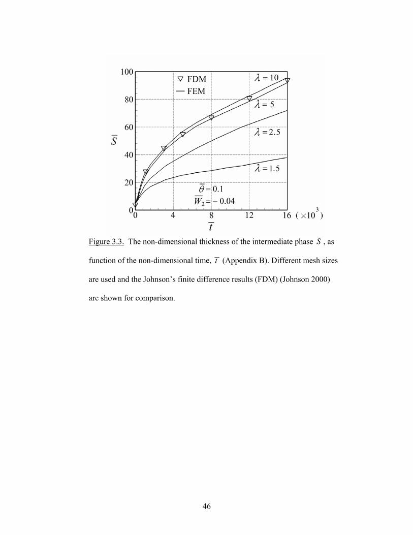
In Figure 3.3, the thickness of the stable ( 0.1)θ = intermediate phase is plotted as

function of time for different mesh densities. By comparing our results to (Johnson

2000) finite difference results, the optimal mesh size seems to be about 51 of the

interface width, i.e., 5=λ . The optimal mesh provides sufficient accuracy with

reasonable computational cost.

The exact solution is unknown. To study the convergence rate, we define the

relative error with respect to the most accurate results )10( =λ . Let ( )S λ , be the

thickness of the intermediate phase. Then the relative error is a function of the non-

dimensional mesh parameter λ :

)10()10()()(

SSSRS

−=

λλ . (3.35)

In Figure 3.4, the relative error is plotted as a function of mesh parameter. The quadratic

convergence is evident.

46

Figure 3.3. The non-dimensional thickness of the intermediate phase S , as

function of the non-dimensional time, t (Appendix B). Different mesh sizes

are used and the Johnson’s finite difference results (FDM) (Johnson 2000)

are shown for comparison.

47

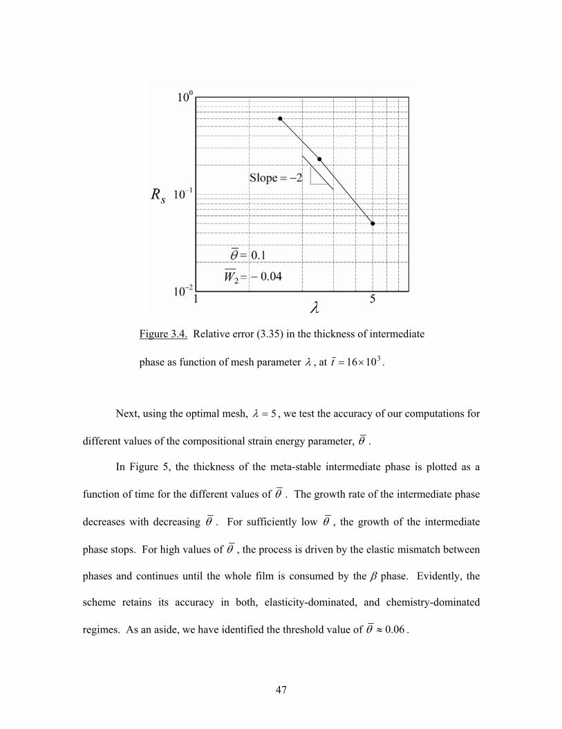
Next, using the optimal mesh, 5=λ , we test the accuracy of our computations for

different values of the compositional strain energy parameter, θ .

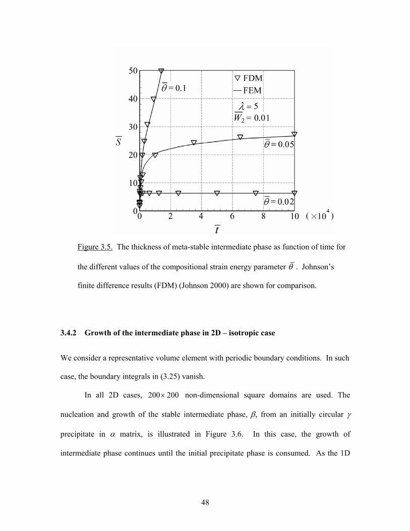
In Figure 5, the thickness of the meta-stable intermediate phase is plotted as a

function of time for the different values of θ . The growth rate of the intermediate phase

decreases with decreasing θ . For sufficiently low θ , the growth of the intermediate

phase stops. For high values of θ , the process is driven by the elastic mismatch between

phases and continues until the whole film is consumed by the β phase. Evidently, the

scheme retains its accuracy in both, elasticity-dominated, and chemistry-dominated

regimes. As an aside, we have identified the threshold value of 0.06θ ≈ .

Figure 3.4. Relative error (3.35) in the thickness of intermediate

phase as function of mesh parameter λ , at 31016 ×=t .

48

3.4.2 Growth of the intermediate phase in 2D – isotropic case

We consider a representative volume element with periodic boundary conditions. In such

case, the boundary integrals in (3.25) vanish.

In all 2D cases, 200200 × non-dimensional square domains are used. The

nucleation and growth of the stable intermediate phase, β, from an initially circular γ

precipitate in α matrix, is illustrated in Figure 3.6. In this case, the growth of

intermediate phase continues until the initial precipitate phase is consumed. As the 1D

Figure 3.5. The thickness of meta-stable intermediate phase as function of time for

the different values of the compositional strain energy parameter θ . Johnson’s

finite difference results (FDM) (Johnson 2000) are shown for comparison.

49

case, we investigate the convergence of the model. The isotopic gradient energy

coefficients, 1K = , and the nominal interface thickness (3.32) is 2.30 ≅l . Initially,

precipitate has circular shape with radius 20 and the final relaxed configuration is a circle

with radius ~ 27.5.

The effects of mesh density and type of element – complete and incomplete – are

shown in Figure 3.7. For the systems with isotropic gradient energy coefficients, the

complete and incomplete elements yield very similar results. The incomplete elements

only slow down the process slightly, but the final configurations are identical. We note

that, in contrast with plate-bending problems, the current isotropic problem does not

include the mixed derivatives of the variable c in its formulation. They only appear in

numerical calculations owing to the different orientation of the element. Thus, the

incompleteness does not obliterate important terms in governing equations (such as

torsional stiffness in plate bending). Hence, its effect is minor. We expect – and indeed

confirm in the next subsection – that the effect is much stronger in the anisotropic case

where mixed derivatives enter the formulation directly.

50

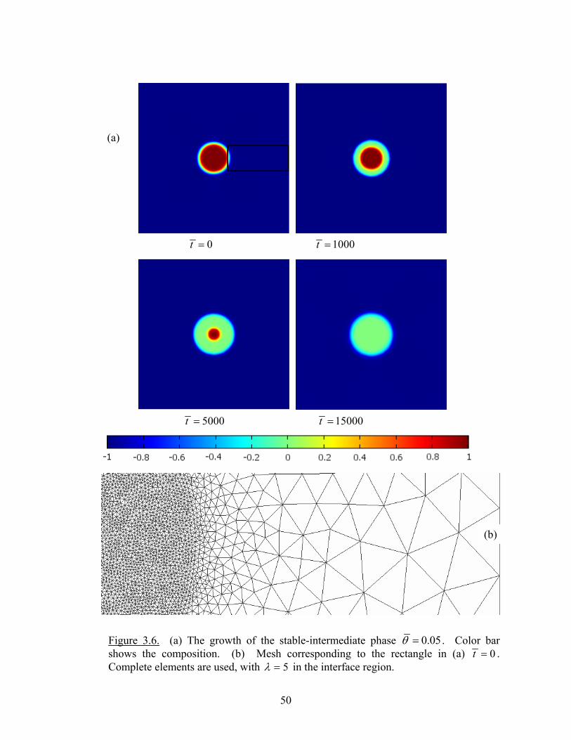
Figure 3.6. (a) The growth of the stable-intermediate phase 0.05θ = . Color bar shows the composition. (b) Mesh corresponding to the rectangle in (a) 0t = . Complete elements are used, with 5=λ in the interface region.

0t = 1000t =

5000t = 15000t =

(a)

(b)

51

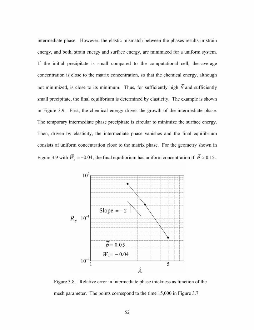
As for 1D systems, the optimal mesh size is about 1/5 of the interface width, i.e.,

5=λ . The relative error is defined as before (3.35), and plotted as function of mesh

parameter (3.34) in Figure 3.8. The results show that the expected quadratic convergence

for 2D systems.

2D problems offer much richer behavior than 1D problems. Consider the

example shown in Figure 3.9. When the intermediate phase is a stable phase (the case

2 0.04W = − in Figure 1), global minimum of chemical energy is achieved at the

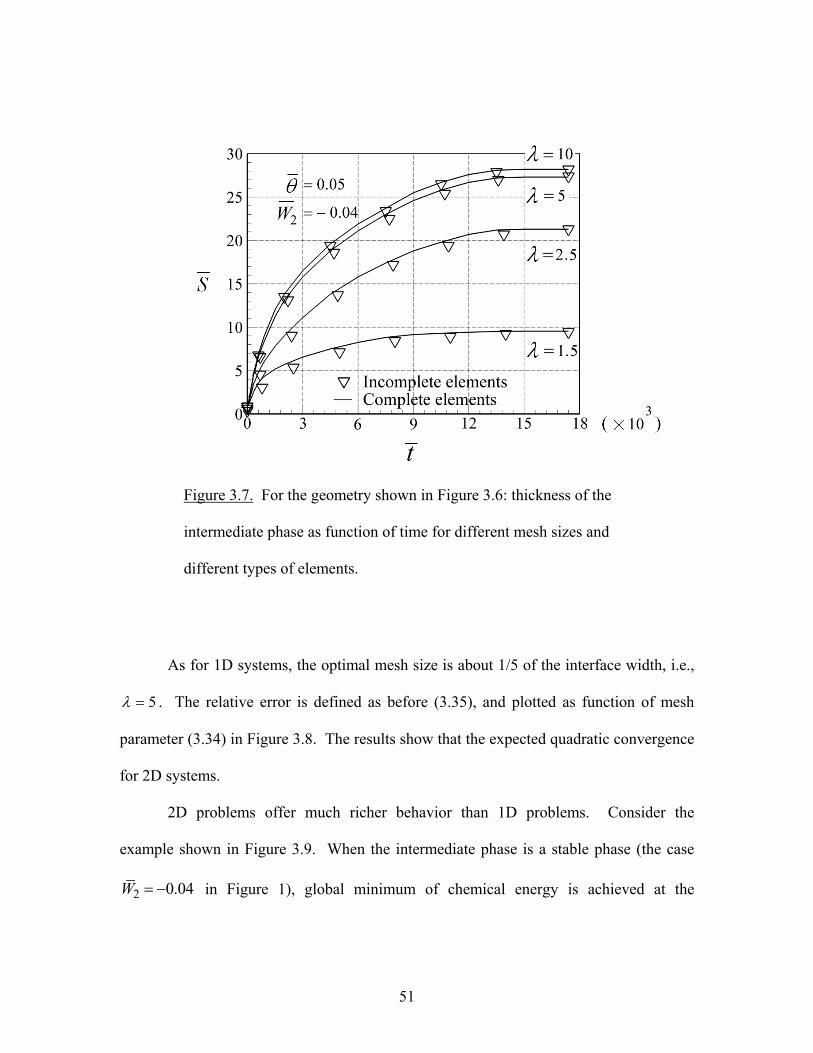
Figure 3.7. For the geometry shown in Figure 3.6: thickness of the

intermediate phase as function of time for different mesh sizes and

different types of elements.

52

intermediate phase. However, the elastic mismatch between the phases results in strain

energy, and both, strain energy and surface energy, are minimized for a uniform system.

If the initial precipitate is small compared to the computational cell, the average

concentration is close to the matrix concentration, so that the chemical energy, although

not minimized, is close to its minimum. Thus, for sufficiently high θ and sufficiently

small precipitate, the final equilibrium is determined by elasticity. The example is shown

in Figure 3.9. First, the chemical energy drives the growth of the intermediate phase.

The temporary intermediate phase precipitate is circular to minimize the surface energy.

Then, driven by elasticity, the intermediate phase vanishes and the final equilibrium

consists of uniform concentration close to the matrix phase. For the geometry shown in

Figure 3.9 with 2 0.04W = − , the final equilibrium has uniform concentration if 0.15θ > .

Figure 3.8. Relative error in intermediate phase thickness as function of the

mesh parameter. The points correspond to the time 15,000 in Figure 3.7.

53

For meta-stable phase intermediate phase (case 2 0.01W = in Figure 3.1), the

behavior is more complicated, as illustrated in Figure 3.10. Consider the geometry with a

circular precipitate shown in Figure 3.6. For 0.02θ < , the growth of intermediate phase

stops before the original precipitate phase is consumed, so that three phases exist in the

final equilibrium of the system. For 0.02 0.05θ< < , intermediate phase completely

consumes the precipitate phase, so that the final equilibrium has only two phases. For

0.05θ > , the temporary intermediate phase continues to transform until the final uniform

state is reached.

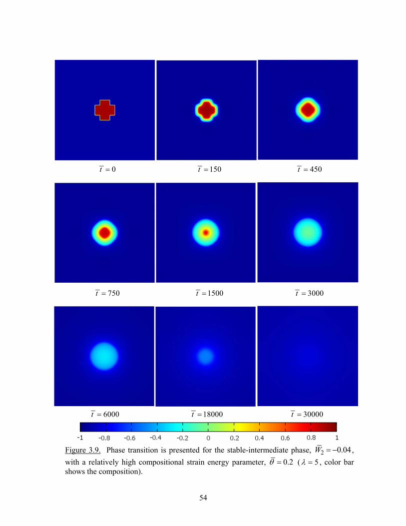
54

0t = 150t = 450t =

750t = 1500t = 3000t =

6000t = 18000t = 30000t =

Figure 3.9. Phase transition is presented for the stable-intermediate phase, 2 0.04W = − ,with a relatively high compositional strain energy parameter, 0.2θ = ( 5=λ , color bar shows the composition).

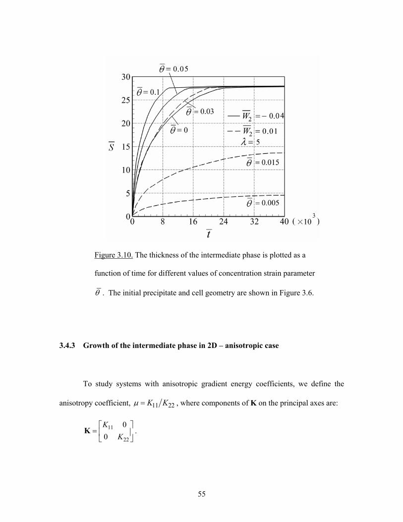
55

3.4.3 Growth of the intermediate phase in 2D – anisotropic case

To study systems with anisotropic gradient energy coefficients, we define the

anisotropy coefficient, 11 22K Kµ = , where components of K on the principal axes are:

11

22

00K

K⎡ ⎤

= ⎢ ⎥⎣ ⎦

K .

Figure 3.10. The thickness of the intermediate phase is plotted as a

function of time for different values of concentration strain parameter

θ . The initial precipitate and cell geometry are shown in Figure 3.6.

56

For arbitrary coordinate system, the off-diagonal components of K will have non-zero

values, so that the mixed derivatives of concentration enter the formulation (3.25)

directly. To ensure sufficiently dense mesh, i.e., at least ten elements ( 5=λ ) across the

interface, the smaller of 11K and 22K is used to calculate the nominal interface thickness

(3.32). The shape evolution of an initially circular precipitate is shown in Figure 3.11,

for a system having stable intermediate phase and anisotropic K matrix, 25.0=µ .

Complete elements are used for this simulation. The initial phase of precipitate vanishes

quickly, but the resulting intermediate phase precipitate then slowly evolves until

reaching its equilibrium elliptical shape.

As expected, in the anisotropic case, the incomplete elements not only slow down

the kinetics but also result in different equilibrium size of the resulting intermediate phase

precipitate. This is illustrated in Figure 3.12, where the longer diameter of the ellipse is

taken to be the measure of the size, S . During the short first phase of the process, while

the initial precipitate phase is consumed by the intermediate phase ( 31015×=t to

31020× depending on µ), the differences in results obtained with complete and

incomplete elements are minor. However, the effect on shape evolution is strong, so that

the error in final configuration, resulting from use of incomplete elements, increases with

increasing anisotropy coefficient.

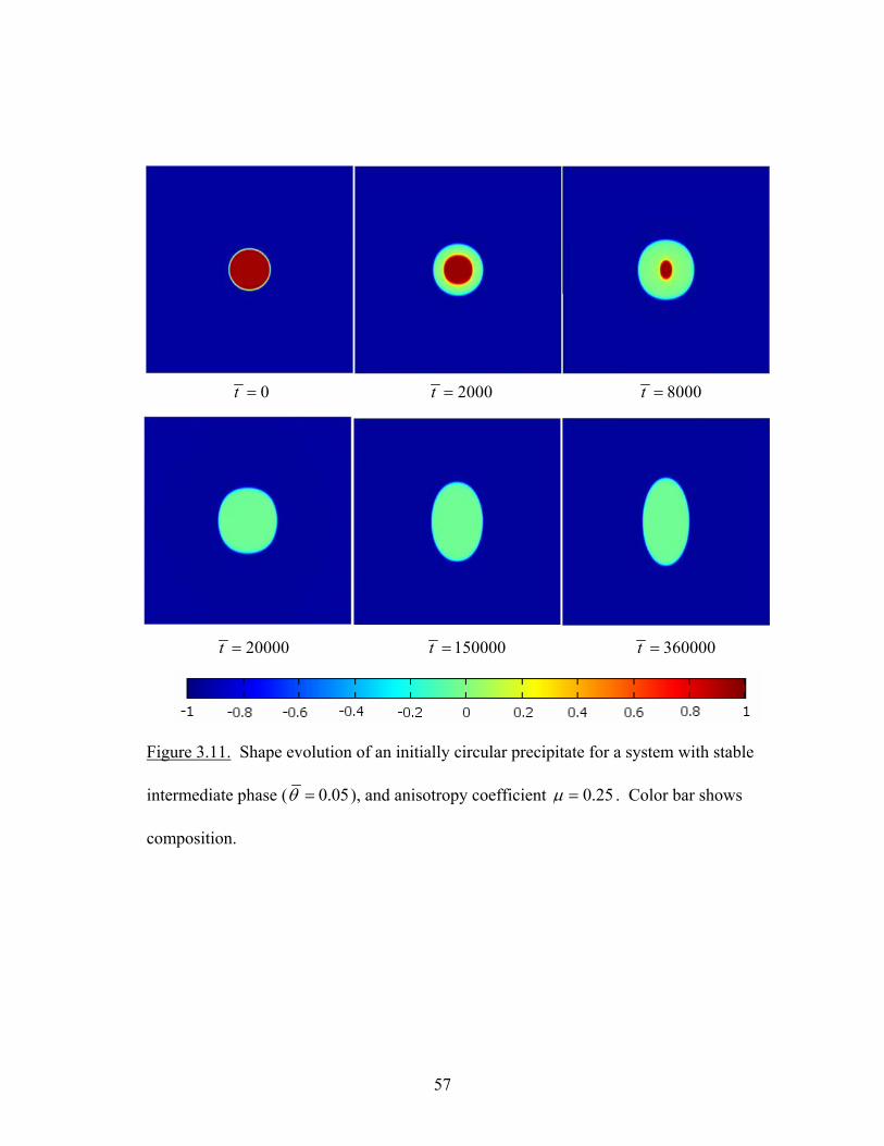
57

0t = 2000t = 8000t =

20000t = 150000t = 360000t =

Figure 3.11. Shape evolution of an initially circular precipitate for a system with stable

intermediate phase ( 0.05θ = ), and anisotropy coefficient 25.0=µ . Color bar shows

composition.

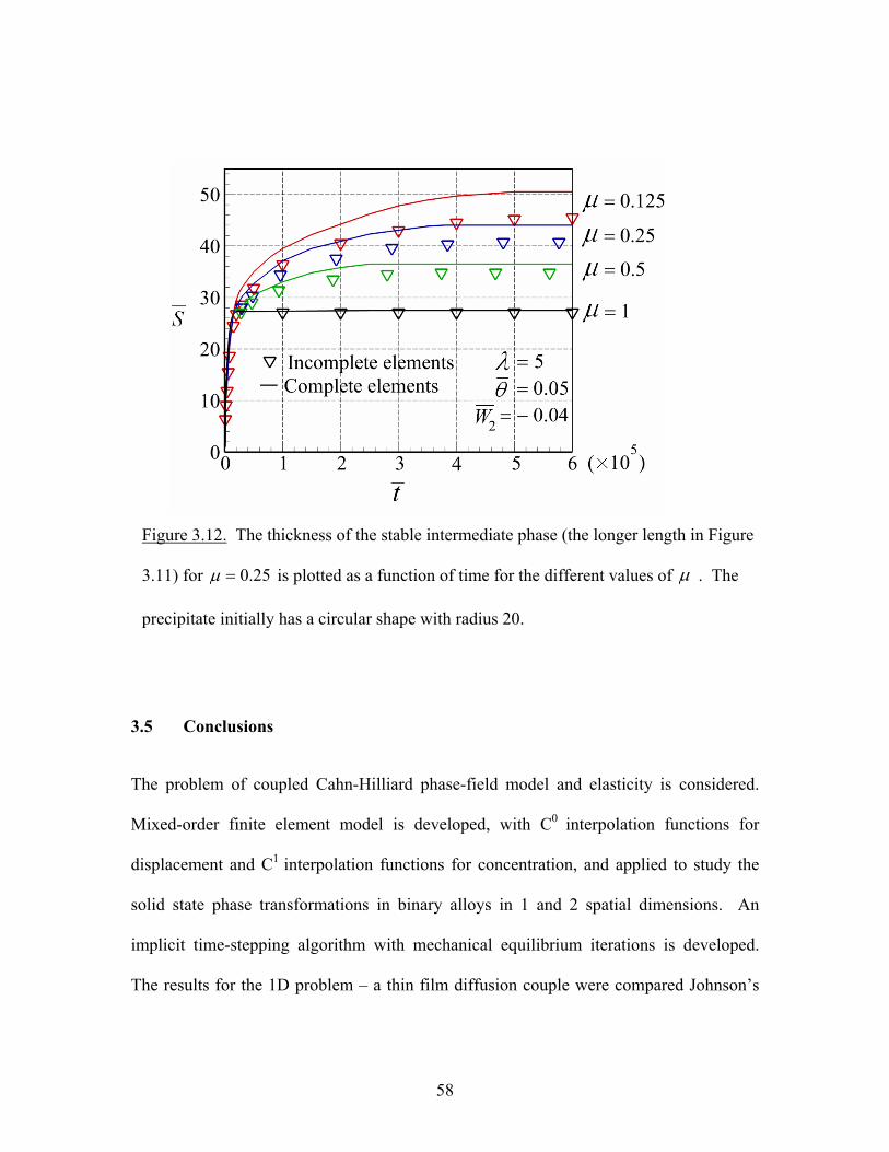
58

3.5 Conclusions

The problem of coupled Cahn-Hilliard phase-field model and elasticity is considered.

Mixed-order finite element model is developed, with C0 interpolation functions for

displacement and C1 interpolation functions for concentration, and applied to study the

solid state phase transformations in binary alloys in 1 and 2 spatial dimensions. An

implicit time-stepping algorithm with mechanical equilibrium iterations is developed.

The results for the 1D problem – a thin film diffusion couple were compared Johnson’s

Figure 3.12. The thickness of the stable intermediate phase (the longer length in Figure

3.11) for 25.0=µ is plotted as a function of time for the different values of µ . The

precipitate initially has a circular shape with radius 20.

59

finite difference results (Johnson 2000). The expected quadratic convergence to the

correct value is confirmed.

In 2D, we also studied the effect of element completeness of interpolation

functions. We used: (a) simple incomplete elements developed as product of Hermit

cubics, and (b) augmented complete elements. Both were developed earlier in the

context of elliptic problems (plate bending), where the inability of incomplete elements to

represent plate torsion proved fatal. In our parabolic problem, the effects of

incompleteness are different.

When the gradient coefficients tensor is isotropic, the incompleteness (i.e., the

lack of ability to describe mixed derivatives) proved to have only a minor effect on

kinetics. This is not surprising since the governing equations do not contain mixed

spatial derivatives of concentration. The equilibrium was reached with very small delay

compared to the results with complete elements. When gradient coefficients tensor is

anisotropic, the governing equations contain mixed derivatives of concentration, so that

the effect of incompleteness is significant. In addition, to the delayed kinetics, the final

equilibrium configurations are also measurably different. The deviations increase with

increasing anisotropy coefficient.

The 2D formulation with complete elements exhibits the expected quadratic

convergence.

In both, 1D and 2D problems, we have studied different regimes, notably the

distinction between chemically energy dominated and elasticity dominated case, as well

60

as different stability of intermediate phases. The developed FE scheme shows consistent

quadratic convergence.

Acknowledgements

This work was supported by USDOE/MICS, grant # DE-FG02-05ER25709.

61

Appendix A

One-dimensional finite element

The coupled mechanical equation (3.16) and phase field /diffusion equation (3.25) are

considered for a thin film diffusion couple. Two-node elements with regular C0

interpolation functions are used to generate the mesh along the plate thickness for

mechanical equation (16). The diffusion/phase field equation is 4th order in

concentration, so the standard convergence theorems require C1 continuity (like beam

elements) (Hughes 2000).

Two-node nonlinear elements with Hermite cubic polynomials are used to

discretize the domain for concentration (3.25). The Hermite cubics in natural coordinates

are given as (Hughes 2000):

1 21 4

1 22 4

1 23 4

1 24 4

( ) ( 1) (2 )

( ) ( 1) ( 1)

( ) ( 1) (2 )

( ) ( 1) ( 1)

H

H

H

H

ξ ξ ξ

ξ ξ ξ

ξ ξ ξ

ξ ξ ξ

= − +

= − +

= + −

= + −

. (A1)

For given nodal values of the concentration and its gradient for a two-node element, the

interpolation within the interval [ 1,1]− is:

ξξξ

ξξξξ

∂∂

++∂∂

+= 2423

1211 )()()()()( cHcHcHcHc , (A2)

62

where 1c and 2c are the concentration at −1 and 1, while 1c ξ∂ ∂ and 2c ξ∂ ∂ are the

gradient of concentration at −1 and 1.

Two-dimensional finite element

For the elasticity equation (3.16), four-node and three-node elements with regular C0

interpolation functions are used to generate the mesh in two dimensions. The

diffusion/phase field equation is 4th order in concentration, so C1 type elements are

required for the convergence (Hughes 2000). We define four-node (rectangular) and

three-node nonlinear elements by using the one dimensional Hermite cubic shape

functions to discretize the two dimensional domain for concentration (3.25).

The interpolation functions for a 2D element must satisfy similar conditions to 1D

interpolation functions. We express the value of the concentration within the 2D quad

element (in natural coordinates) as:

∑=

−−−⎥⎥⎦

⎤

⎢⎢⎣

⎡Ψ

∂∂∂

+Ψ∂∂

+Ψ∂

∂+Ψ=

4

14

2

142434 ),(),(),(),(),(n

nn

nn

nn

nnccc

cc ηξηξ

ηξη

ηξξ

ηξηξ .

(A3)

To construct the interpolation functions, we note that for (A3) to be true, they

must satisfy conditions similar to those satisfied by 1D interpolation functions (Hermite

cubics), i.e., the value that corresponds to the particular degree of freedom (DOF) at

particular node must be one, while all other values that correspond to other DOFs at the

same or other node, must be zero. That can be achieved by making products of the type

63

)()( ηξ ji HH . Such products will form 6th order polynomials in ),( ηξ . The interpolation

functions for a rectangular element are (Chien and Shih 2009):

5 3 11 1 1

6 4 12 2 1

3 1 2 7 3 2

4 2 2 8 4 2

9 3 3

10

( , ) ( ) ( )( , ) ( ) ( )( , ) ( ) ( )( , ) ( ) ( )

1: 2 :( , ) ( ) ( ) ( , ) ( ) ( )( , ) ( ) ( ) ( , ) ( ) ( )

( , ) ( ) ( )( ,

3 :

H HH HH HH H

node nodeH H H HH H H H

H H

node

ξ η ξ ηξ η ξ ηξ η ξ ηξ η ξ η

ξ η ξ η ξ η ξ ηξ η ξ η ξ η ξ η

ξ η ξ ηξ

Ψ =Ψ = ⎧⎧⎪⎪ Ψ =Ψ =⎪ ⎪

⎨ ⎨Ψ = Ψ =⎪ ⎪⎪ ⎪Ψ = Ψ =⎩ ⎩

Ψ =

Ψ13 1 3

14 2 34 3

15 1 413 1 2

16 2 412 4 4

( , ) ( ) ( )( , ) ( ) ( )) ( ) ( )

4 :( , ) ( ) ( )( , ) ( ) ( )( , ) ( ) ( )( , ) ( ) ( )

H HH HH H

nodeH HH HH HH H

ξ η ξ ηξ η ξ ηη ξ ηξ η ξ ηξ η ξ ηξ η ξ ηξ η ξ η

Ψ =⎧⎧⎪⎪ Ψ ==⎪ ⎪

⎨ ⎨Ψ =Ψ =⎪ ⎪⎪ ⎪Ψ =Ψ =⎩ ⎩

(A4)

For the incomplete element, which does not include the mixed derivatives, the last

terms in (A3) vanish, so that the interpolation functions 4Ψ , 8Ψ , 12Ψ , and 16Ψ do not

enter the formulation. The interpolation functions for a triangular element are derived

from the quad interpolation functions by the standard node-coincidence method (Hughes

2000).

64

Appendix B

The particular dimensional reduction has been used by (Johnson 2000). It is rendered

unique by two requirements. First – that the re-scaled composition c varies between −1

and 1, with intermediate phase at 0c β = . Therefore:

)(2

αγ

αγ

mm

mm

ccccc

c−

−−= . (B1)

Second – that the non-dimensional gradient coefficient is 1K = , in the isotropic case.

The non-dimensional and scaled variables are identified by overbars.

With these requirements, the characteristic length L, the characteristic time Ω ,

and the characteristic energy density W , are:

( )

8

20

2

0

22

,2⎟⎟

⎠

⎞

⎜⎜

⎝

⎛

−=

⎟⎟

⎠

⎞

⎜⎜

⎝

⎛

−= αγαγ ρρ cckTB

KΩcckT

KX ,

6

0 2 ⎟⎟

⎠

⎞

⎜⎜

⎝

⎛ −=

αγ

ρcc

kTW . (B2)

In (B2) 0ρ is density of the lattice sites, k is Boltzmann’s constant, and T is the

temperature. The non-dimensional gradient energy coefficient, K , becomes 1 for all

isotropic systems. For 2D systems with anisotropic gradient energy coefficients, we keep

122 =K , and vary 11K .

Considering isotropic mobility, the non-dimensional flux is:

65

5

00

2⎟⎟

⎠

⎞

⎜⎜

⎝

⎛

−= αγρ ccBWA

qq , (B3)

so that non-dimensional mobility coefficient, 1B = .

66

CHAPTER FOUR: Morphological Instabilities in Thin Films

(Submitted to Acta Materialia, 2010)

Mohsen Asle Zaeem and Sinisa Dj. Mesarovic

School of Mechanical and Materials Engineering, Washington State University, Pullman,

WA, 99164 USA

Abstract

Cahn-Hilliard type of phase-field model coupled with elasticity equations is used to study

the instability of multilayer thin film diffusion couples in solid state. A mixed order finite

element model which we previously developed for solving the coupled phase-field and

mechanical governing equations is used for the computations. Maps of transformations in

multilayer systems are carried out considering the effects of thickness of layers, volume

fraction of films, and compositional strain on the instability of the multilayer thin films. It

is shown that at some cases phase transformation, intermediate phase nucleation and

growth, or deformation of layers due to high compositional strain can lead to the

coarsening of the layers which can result in different mechanical and materials behaviors

of the original designed multilayer.

Key words: Phase field modeling, elasticity, multilayer thin films, instability

67

4.1 Introduction

Multilayer thin films have been a very active research area in the past decade. When the

thickness of individual layer is reduced to micro- or nano-scale, novel mechanical

(Jankowski 1995; Movchan and Lemkey 1997; McKeown et al. 2002; Eizadjou et al.

2008; Mara 2004), optical (Atkinson and Dodd 1997), electronic (Stobiecki et al. 1998;

Czapkiewicz et al. 1996), and magnetic (Atkinson and Dodd 1997; Stobiecki et al. 1998;

Czapkiewicz et al. 1996) properties emerge, which make such materials attractive for a

number of potential applications. In multilayer micro- and nano-films, the stability of

phases is required to maintain the desirable properties. For example, significant drop of

hardness occurs after annealing of Ni/Ru multilayers at 600 Co (Wen et al. 2008).

Different temperature or stress fields may result in instability of multilayers. For

example breakdown of the Ni layers happens when multilayer Ni/Ag is annealed at

600 Co (Lewis et al. 2003), and pinch-off (holes in grain boundary triple junctions) of Co

layers in Co/Cu multilayers is observed after creep test at 830 Co (Josell et al. 1999).

(Greer 1986 and 1993) classified the changes that can occur in thin film

multilayers as their microstructures evolve. He divided these processes to the following

categories: inter-diffusion (same phases coexist with changed compositions) (Ag/Au

(Yang and Greer 1996), Ni/Al and Ag/Zn (Ghosh and Paul 2007), Al/Ni (Grag et al.

1999)), interfacial reaction (nucleation and growth of a new phase) (Si/Ni (Gosele and Tu

1982), Ni/Zr (Highmore et al. 1987), Al/Mn (Srivastava et al. 2007), Ni/Al (Noro et al.

2008)), transformation in one phase of the multilayer without any changes in other

68

phase(s)(Si/Al (Konno et al. 1992)), and, coarsening or spinodal decomposition of the

layers (Ni/Ag (Wen et al. 2008), Ni/C (Chernov et al. 2000)).

In solid state, microstructural evolution can be affected by elasticity of the

system; the lattice continuity across the interfaces between mismatched phases produces

elastic strains and can have significant effects on the stability of the multilayered systems

(Larche and Cahn 1978 and 1992; Cahn and Larche 1982; Grinfeld 1986; Srolovitz 1989;

Chirranjeevi et al. 2009).

The theory of phase transition and spinodal decomposition in solid state was

developed by (Cahn and Hilliard 1958). The numerical studies in the area of solid state

phase transformation are mostly based on diffusive-interface or phase-field models

(Kassner et al. 2001; Leo and Johnson 2001; Wang et al. 2004; Chen et al. 1991; Wang et

al. 1993; Wang and Khachaturyan 1995; Chen and Shen 1998; Hu and Chen 2001;

Vaithyanathan et al. 2004; Cahn and Kobayashi 1995; Johnson 2000; Seol et al. 2005;

Yeon et al. 2006; Ratz et al. 2006). Among these studies, a few looked at thin films

which either are one-dimensional models (Cahn and Kobayashi 1995; Johnson 2000)

which can not predict all the possible phase transformations in multilayers, or are focused

on the films and fluid interactions (Seol et al. 2005; Yeon et al. 2006; Ratz et al. 2006).

Recently, (Chirranjeevi et al. 2009 ) used a phase field model to study the instability of a

special two-phase multilayer with one phase much stiffer than the other.

Here, we present a comprehensive study of binary multilayer thin films, including

the two-phase systems, and systems with an intermediate phase (meta-stable or stable).

Following the dimensional analysis, we develop the maps of the evolution behavior of

69

multilayers, including the effects of initial geometry and elasticity of the system. We use

the recently developed Galerkin finite element formulation (Asle Zaeem and Mesarovic

2009 and 2010) of the Cahn-Hilliard diffuse interface model (Cahn and Hilliard 1958),

coupled with elasticity (Johnson 2000 ).

The paper is organized as follows. In Section 2, formulation, dimensional

analysis and numerical solver for the coupled phase filed-elasticity equations are

presented; the maps of transformations for two-phase systems, systems with stable

intermediate phase, and systems with meta-stable intermediate phase are presented in

Sections 3, 4 and 5, respectively; a short conclusion is presented in Section 6.

4.2 Formulation and Numerical Method

In solid state phase transformations, the lattice continuity across the interfaces between

mismatched phases produces elastic strains (Cahn and Larche 1982; Larche and Cahn

1992), so that the 2nd order elasticity PDEs need to be coupled to the phase field equation

(Leo and Johnson 2001; Cahn and Kobayashi 1995; Johnson 2000). Phase field models

are characterized by the dependence of the free energy of a non-uniform system on the

phase field variable (e.g., composition, c). In this work, a binary system is considered,

with components A and B, which forms three phases (α , β , and γ ), and characterized

by the molar fraction of the component A, c. The total free energy, F, of a non-

homogeneous system with volume V, bounded by surface S, is constructed as:

70

∫−∫ ∇++=S

iiV

iji SdutdVccUcfucF ])(2

),()([),( 2κε . (4.1)

)(cf is the stress-free Helmholtz free energy density of a uniform system. κ is the

isotropic gradient energy coefficient. it is the surface traction component, and iu is the

displacement component. In (4.1), the surface energy of the outer boundary S is

neglected. ),( cU ijε is the strain energy density and ijε is the total strain tensor:

ijeijijjiij euu δεε +=+= )(

21

,, , (4.2)

where iu is the displacement component, eijε is the elastic strain and e is the purely

volumetric compositional strain. The simplest model follows the linear Vegard’s law

(Denton and Ashcroft 1991):

0( )e c cη= - . (4.3)

The reference composition 0c is taken to be the average of composition over the domain.

η is the compositional strain parameter.

For solid state phase transformation, the phase-field variable is subject to a

conservation law. This kind of conserved phase field formulations results in a 4th order

evolution PDE (Asle Zaeem and Mesarovic 2010):

MBc 2∇=& , (4.4)

where B is the isotropic mobility coefficient, and the chemical potential, M, is equal to

the variational derivative of the free energy respect to composition (Larche and Cahn

1978):

71

cUfM 2∇−′−′= κ . (4.5)

The Helmholtz free energy density of a uniform unstressed system, )(cf in (4.1),

is assumed to be a triple well potential that can produce binary systems with no-

intermediate phase, stable intermediate phase, and meta-stable intermediate phase:

222

2221 )()()()()()( γαγβα ccccWccccccWcf −−+−−−= , (4.6)

where 1W and 2W are the energy coefficients, αc , βc and γc are the mole fractions of

component B at which )(cf is minimized.

By using a particular dimensional reduction (Johnson 2000; Asle Zaeem and

Mesarovic 2010) we can find the non-dimensional independent parameters of the system.

The scaled composition, c , varies between 1−=αc and 1−=γc , with intermediate

phase at 0=βc :

)(

2αγ

αγ

cc

cccc

−

−−= . (4.7)

The characteristic length X, the characteristic time Ω , and the characteristic energy

density W , are:

2

0

2

⎟⎟⎟

⎠

⎞

⎜⎜⎜

⎝

⎛

−=

αγρκ

cckTX , (4.8a)

( )

8

20

22 ⎟

⎟⎟

⎠

⎞

⎜⎜⎜

⎝

⎛

−=

αγρ

κ

cckTBΩ , (4.8b)

72

6

0 2 ⎟⎟

⎠

⎞

⎜⎜

⎝

⎛ −=

αγ

ρcc

kTW , (4.8c)

where 0ρ is density of the lattice sites, k is Boltzmann’s constant, and T is the

temperature. κ affects only the length and time scale, and B affects only the time scale

(non-dimensional gradient energy coefficient and mobility are 1== Bκ for isotropic

cases). Therefore, their variations in numerical runs are superfluous. One only needs to

rescale length and time in the solution to get the results. The scaled compositional strain

parameter is:

2

0

2)1( ⎟

⎟

⎠

⎞

⎜⎜

⎝

⎛

−−= αγρ

ηηccvkT

E , (4.9)

where E is the Young’s modulus, and v is the Poisson ratio (in this paper 3.0=v ). The

non-dimensional elastic modulus are: )21)(1(

)1( 211 vv

vC−+

−= ,

)21)(1()1(

12 vvvvC−+

−= , and

)1()1(

44 vvC

+−

= . By applying this particular dimensional reduction all the parameters of the

system will be reduced to three independent non-dimensional parameters, η , WWW 1

1 =

and WWW 2

2 = . By varying 1W and 2W in (4.6), we can produce different binary alloy

systems with no-intermediate phase ( 01 =W and 02.02 =W ), stable intermediate phase

( 4.01 =W and 04.02 −=W ), and meta-stable intermediate phase ( 4.01 =W and

02.02 =W ), which are shown in Figure 1, and β is the intermediate phase.

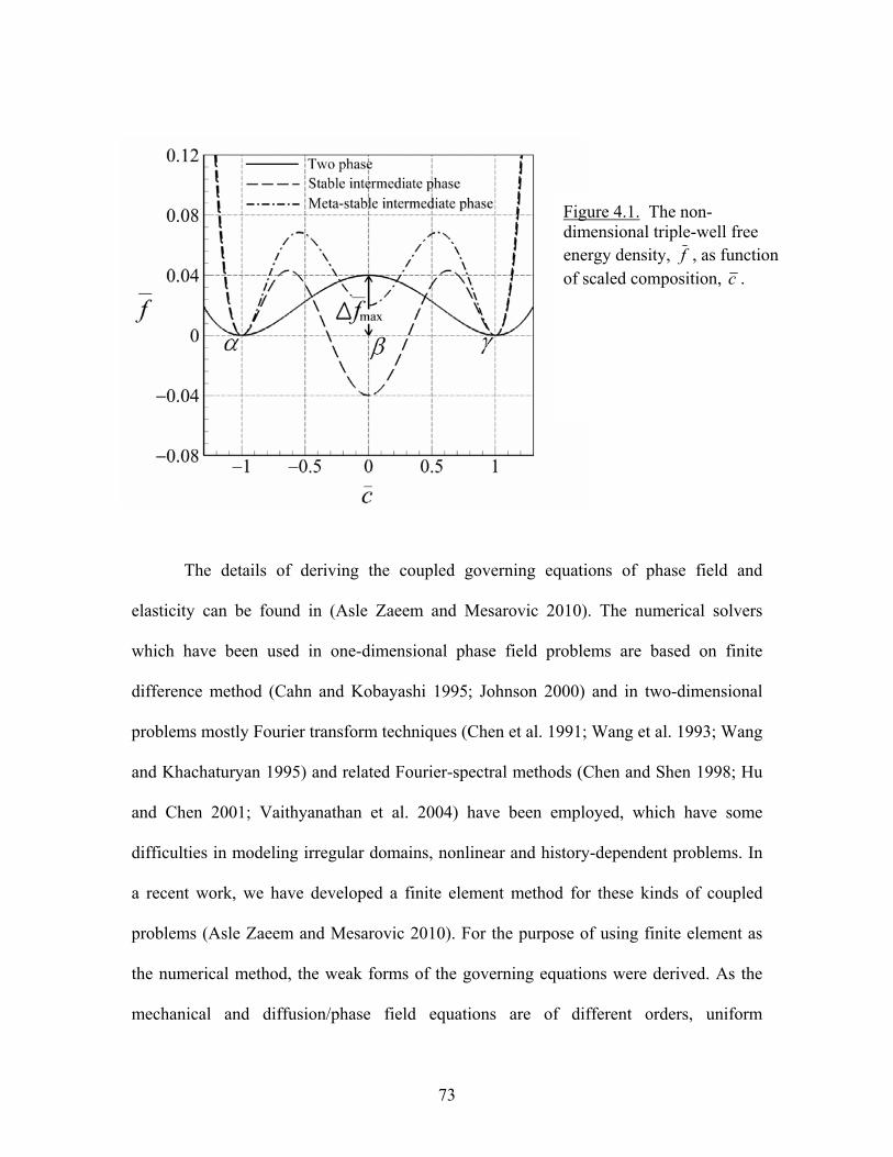
73

The details of deriving the coupled governing equations of phase field and

elasticity can be found in (Asle Zaeem and Mesarovic 2010). The numerical solvers

which have been used in one-dimensional phase field problems are based on finite

difference method (Cahn and Kobayashi 1995; Johnson 2000) and in two-dimensional

problems mostly Fourier transform techniques (Chen et al. 1991; Wang et al. 1993; Wang

and Khachaturyan 1995) and related Fourier-spectral methods (Chen and Shen 1998; Hu

and Chen 2001; Vaithyanathan et al. 2004) have been employed, which have some

difficulties in modeling irregular domains, nonlinear and history-dependent problems. In

a recent work, we have developed a finite element method for these kinds of coupled

problems (Asle Zaeem and Mesarovic 2010). For the purpose of using finite element as

the numerical method, the weak forms of the governing equations were derived. As the

mechanical and diffusion/phase field equations are of different orders, uniform

Figure 4.1. The non-dimensional triple-well free energy density, f , as function of scaled composition, c .

74

convergence of the results requires different order of continuity for interpolation

functions (Hughes 2000). We formulated and implemented such mixed-order finite

elements, with C0 interpolation functions for displacement, and C1 interpolation functions

for composition. A special time integration scheme was developed consisting of implicit

time-stepping and equilibrium/consistency iterations in each time step. Special boundary

settings are considered to simulate the multilayer thin films, and for all of our 2D cases,

left and right boundaries have periodic boundary condition and top and bottom

boundaries have no-traction and no-flux boundary conditions (shown in Figure 4.2).

For the finite element mesh, the optimal mesh size was determined to be about 1/5

of the interface width which it guarantees the uniform quadratic convergence, expected

for conforming elements (Asle Zaeem and Mesarovic 2010). The nominal interface

thickness (for coexisting isotropic phases α and γ) is derived by (Cahn and Hilliard

1958]:

21

max0 2

)( ⎟⎟⎠

⎞⎜⎜⎝

⎛∆

−=fKccl αγ , (4.10)

where maxf∆ is the difference between the neighboring maximum and minimum of the

free energy (4.6), as illustrated in Figure 4.1.

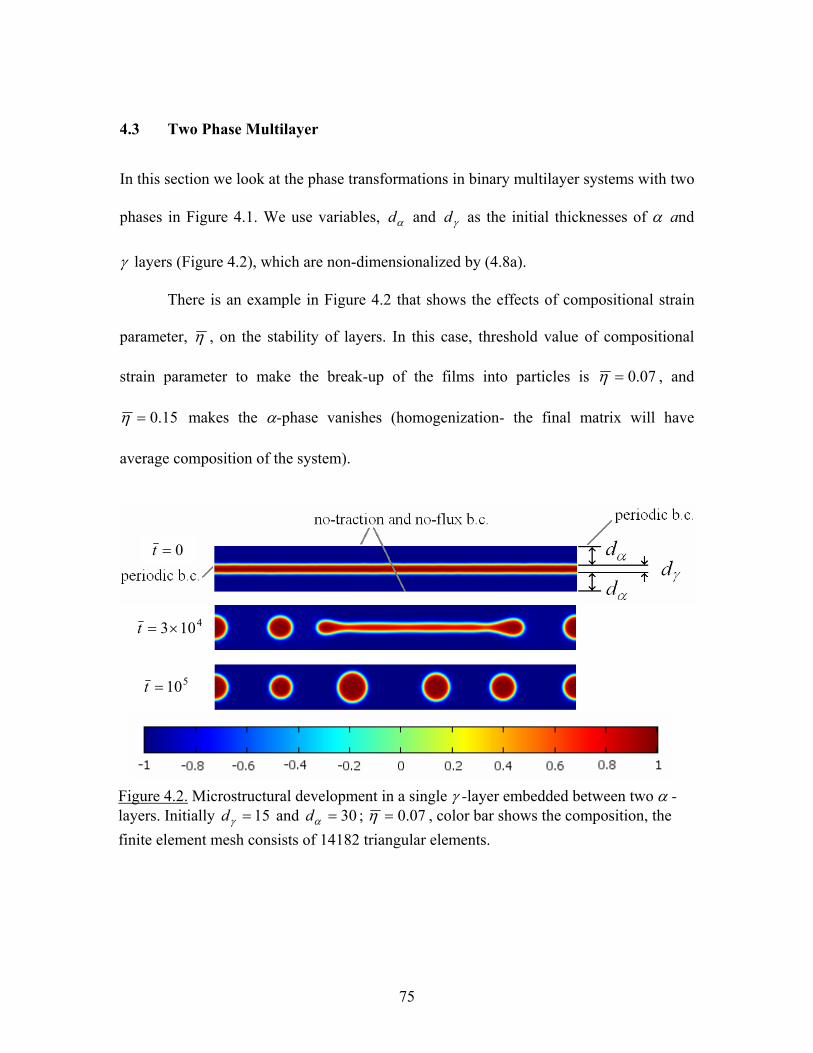
75

4.3 Two Phase Multilayer

In this section we look at the phase transformations in binary multilayer systems with two

phases in Figure 4.1. We use variables, αd and γd as the initial thicknesses of α and

γ layers (Figure 4.2), which are non-dimensionalized by (4.8a).

There is an example in Figure 4.2 that shows the effects of compositional strain

parameter, η , on the stability of layers. In this case, threshold value of compositional

strain parameter to make the break-up of the films into particles is 07.0=η , and

15.0=η makes the α-phase vanishes (homogenization- the final matrix will have

average composition of the system).

Figure 4.2. Microstructural development in a single γ -layer embedded between two α -layers. Initially 15=γd and 30=αd ; 07.0=η , color bar shows the composition, the finite element mesh consists of 14182 triangular elements.

4103×=t

510=t

0=t

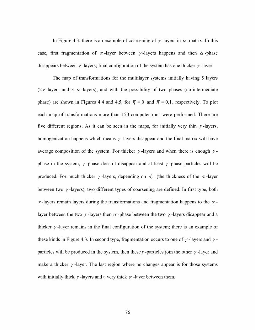
76

In Figure 4.3, there is an example of coarsening of γ -layers in α -matrix. In this

case, first fragmentation of α -layer between γ -layers happens and then α -phase

disappears between γ -layers; final configuration of the system has one thicker γ -layer.

The map of transformations for the multilayer systems initially having 5 layers

(2γ -layers and 3 α -layers), and with the possibility of two phases (no-intermediate

phase) are shown in Figures 4.4 and 4.5, for 0=η and 1.0=η , respectively. To plot

each map of transformations more than 150 computer runs were performed. There are

five different regions. As it can be seen in the maps, for initially very thin γ -layers,

homogenization happens which means γ -layers disappear and the final matrix will have

average composition of the system. For thicker γ -layers and when there is enough γ -

phase in the system, γ -phase doesn’t disappear and at least γ -phase particles will be

produced. For much thicker γ -layers, depending on αd (the thickness of the α -layer

between two γ -layers), two different types of coarsening are defined. In first type, both

γ -layers remain layers during the transformations and fragmentation happens to the α -

layer between the two γ -layers then α -phase between the two γ -layers disappear and a

thicker γ -layer remains in the final configuration of the system; there is an example of

these kinds in Figure 4.3. In second type, fragmentation occurs to one of γ -layers and γ -

particles will be produced in the system, then theseγ -particles join the other γ -layer and

make a thicker γ -layer. The last region where no changes appear is for those systems

with initially thick γ -layers and a very thick α -layer between them.

77

Figure 4.4. Map of transformations for the systems with possibility of two phases (no-intermediate phase) and 0=η . The non-dimensional interface thickness calculated form (4.10) is 70 ≅l . All the

results are from 710=t .

4109×=t 41012 ×=t

Figure 4.3. Coarsening of γ -layers. Initially 25=γd and 15=αd ; 1.0=η , and color bar shows the composition. The finite element mesh consists of 22248 triangular elements.

0=t 4107.8 ×=t

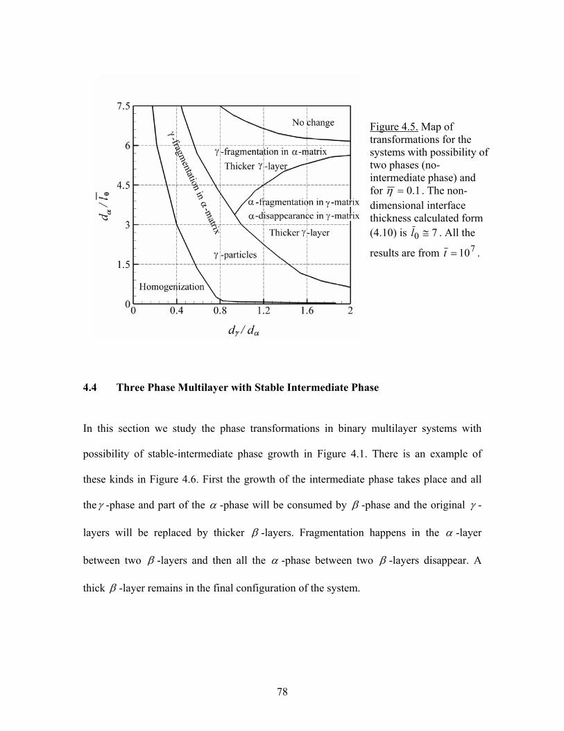
78

4.4 Three Phase Multilayer with Stable Intermediate Phase

In this section we study the phase transformations in binary multilayer systems with

possibility of stable-intermediate phase growth in Figure 4.1. There is an example of

these kinds in Figure 4.6. First the growth of the intermediate phase takes place and all

theγ -phase and part of the α -phase will be consumed by β -phase and the original γ -

layers will be replaced by thicker β -layers. Fragmentation happens in the α -layer

between two β -layers and then all the α -phase between two β -layers disappear. A

thick β -layer remains in the final configuration of the system.

Figure 4.5. Map of transformations for the systems with possibility of two phases (no-intermediate phase) and for 1.0=η . The non-dimensional interface thickness calculated form (4.10) is 70 ≅l . All the

results are from 710=t .

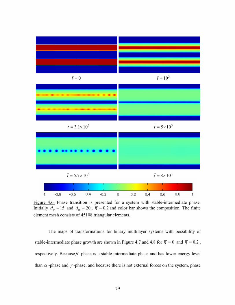
79

The maps of transformations for binary multilayer systems with possibility of

stable-intermediate phase growth are shown in Figure 4.7 and 4.8 for 0=η and 2.0=η ,

respectively. Because β -phase is a stable intermediate phase and has lower energy level

than α -phase and γ -phase, and because there is not external forces on the system, phase

0=t 310=t

3101.3 ×=t 3105×=t

3107.5 ×=t 3108×=t

Figure 4.6. Phase transition is presented for a system with stable-intermediate phase. Initially 15=γd and 20=αd ; 2.0=η and color bar shows the composition. The finite element mesh consists of 45108 triangular elements.

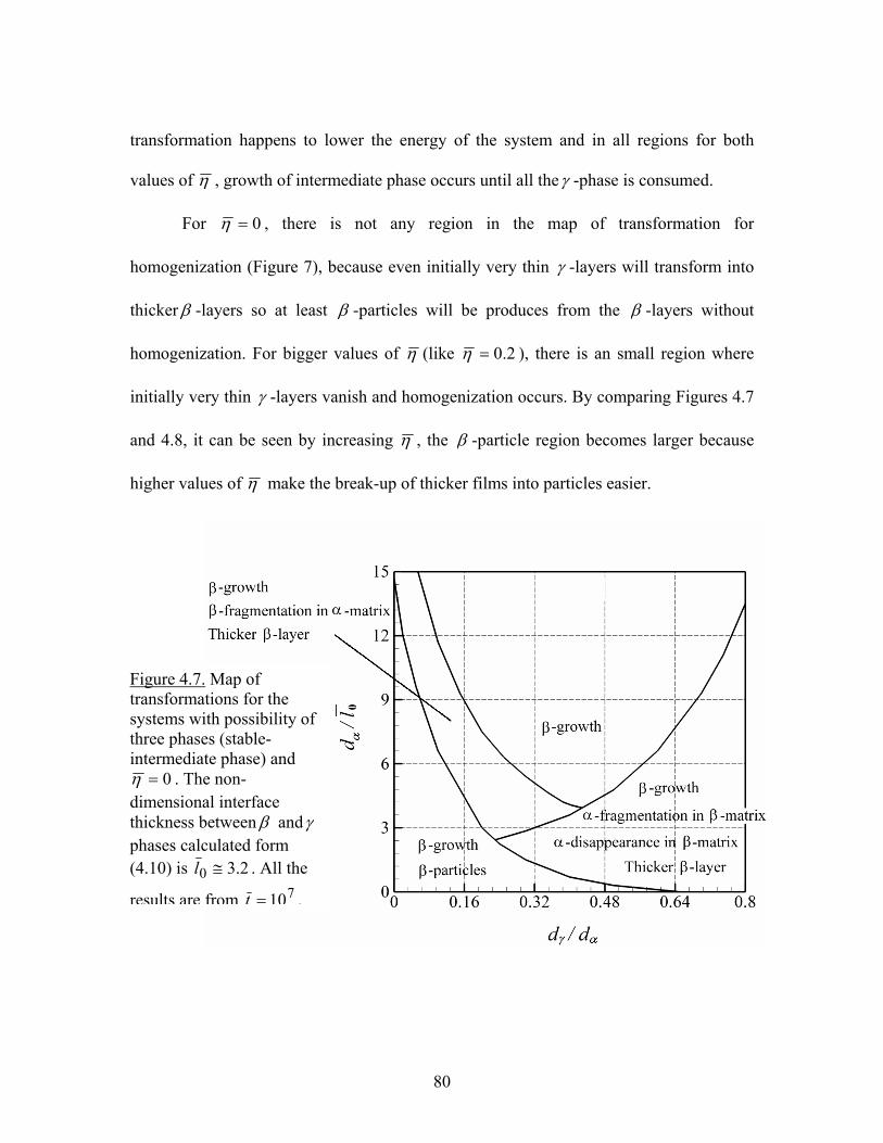
80

transformation happens to lower the energy of the system and in all regions for both

values of η , growth of intermediate phase occurs until all theγ -phase is consumed.

For 0=η , there is not any region in the map of transformation for

homogenization (Figure 7), because even initially very thin γ -layers will transform into

thicker β -layers so at least β -particles will be produces from the β -layers without

homogenization. For bigger values of η (like 2.0=η ), there is an small region where

initially very thin γ -layers vanish and homogenization occurs. By comparing Figures 4.7

and 4.8, it can be seen by increasing η , the β -particle region becomes larger because

higher values of η make the break-up of thicker films into particles easier.

Figure 4.7. Map of transformations for the systems with possibility of three phases (stable-intermediate phase) and

0=η . The non-dimensional interface thickness between β andγ phases calculated form (4.10) is 2.30 ≅l . All the

results are from 710=t .

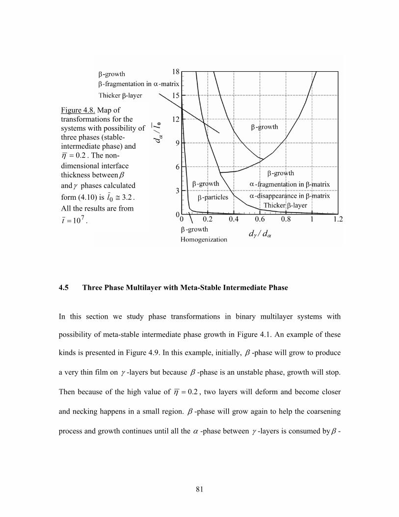
81

4.5 Three Phase Multilayer with Meta-Stable Intermediate Phase

In this section we study phase transformations in binary multilayer systems with

possibility of meta-stable intermediate phase growth in Figure 4.1. An example of these

kinds is presented in Figure 4.9. In this example, initially, β -phase will grow to produce

a very thin film on γ -layers but because β -phase is an unstable phase, growth will stop.

Then because of the high value of 2.0=η , two layers will deform and become closer

and necking happens in a small region. β -phase will grow again to help the coarsening

process and growth continues until all the α -phase between γ -layers is consumed by β -

Figure 4.8. Map of transformations for the systems with possibility of three phases (stable-intermediate phase) and

2.0=η . The non-dimensional interface thickness between β andγ phases calculated form (4.10) is 2.30 ≅l . All the results are from

710=t .

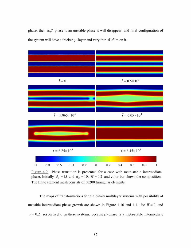
82

phase, then as β -phase is an unstable phase it will disappear, and final configuration of

the system will have a thicker γ -layer and very thin β -film on it.

The maps of transformations for the binary multilayer systems with possibility of

unstable-intermediate phase growth are shown in Figure 4.10 and 4.11 for 0=η and

2.0=η , respectively. In these systems, because β -phase is a meta-stable intermediate

0=t 3105.0 ×=t

410865.5 ×=t 41005.6 ×=t

41025.6 ×=t 41045.6 ×=t

Figure 4.9. Phase transition is presented for a case with meta-stable intermediate phase. Initially 15=γd and 10=αd ; 2.0=η and color bar shows the composition. The finite element mesh consists of 50200 triangular elements

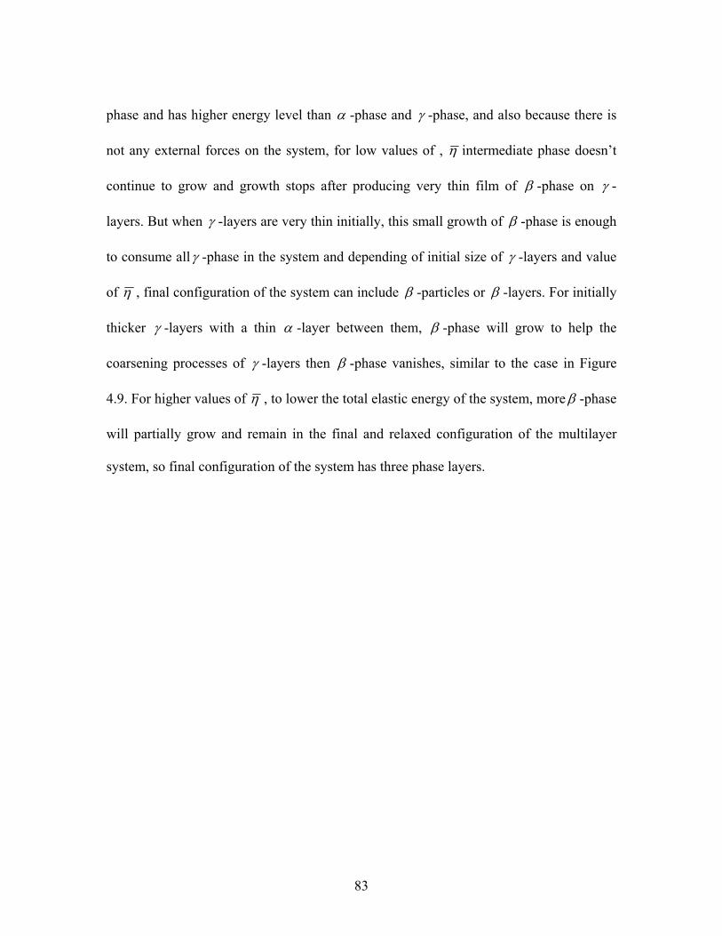
83

phase and has higher energy level than α -phase and γ -phase, and also because there is

not any external forces on the system, for low values of , η intermediate phase doesn’t

continue to grow and growth stops after producing very thin film of β -phase on γ -

layers. But when γ -layers are very thin initially, this small growth of β -phase is enough

to consume allγ -phase in the system and depending of initial size of γ -layers and value

of η , final configuration of the system can include β -particles or β -layers. For initially

thicker γ -layers with a thin α -layer between them, β -phase will grow to help the

coarsening processes of γ -layers then β -phase vanishes, similar to the case in Figure

4.9. For higher values of η , to lower the total elastic energy of the system, more β -phase

will partially grow and remain in the final and relaxed configuration of the multilayer

system, so final configuration of the system has three phase layers.

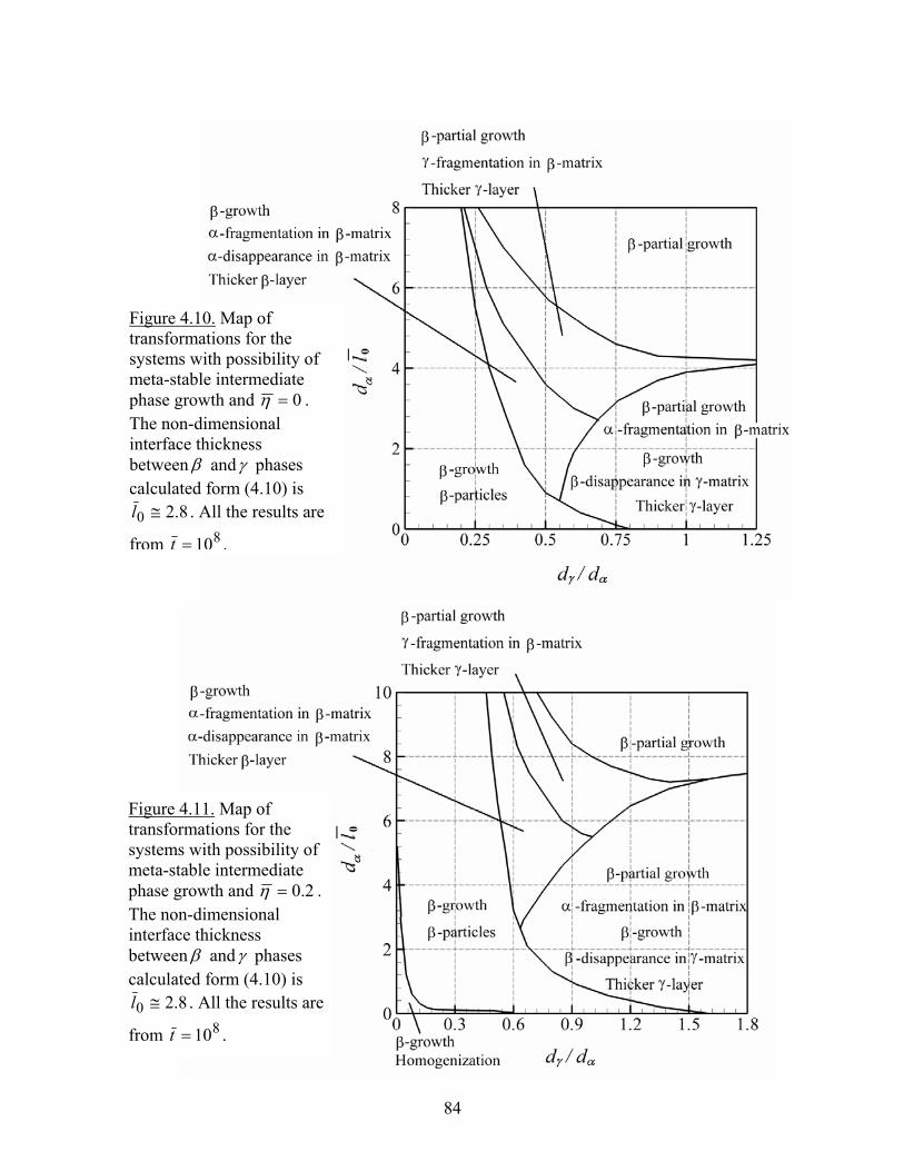
84

Figure 4.10. Map of transformations for the systems with possibility of meta-stable intermediate phase growth and 0=η . The non-dimensional interface thickness between β andγ phases calculated form (4.10) is

8.20 ≅l . All the results are

from 810=t .

Figure 4.11. Map of transformations for the systems with possibility of meta-stable intermediate phase growth and 2.0=η . The non-dimensional interface thickness between β andγ phases calculated form (4.10) is

8.20 ≅l . All the results are

from 810=t .

85

4.6 Conclusion

Maps of transformations for multilayer thin films are carried out considering the effects

of thickness of layers, volume fraction of films, and compositional strain on the

instability of the multilayer system. Three different binary systems are considered

representing multilayer thin films with no-intermediate phase, stable intermediate phase,

and meta-stable intermediate phase. It is shown that at some cases phase transformation,

intermediate phase nucleation and growth, or fragmentation of layers due to high

compositional strain can result in instability of multilayer thin films.

Although, without considering the effects of compositional strain on the

multilayer systems we can determine the map of transformations, but from our results it

is clear that the elastic force coming from compositional strain is an effective factor to

make the multilayer unstable and can change the map of transformations significantly.

86

CHAPTER FIVE: Summary and Future Works

The problem of coupled Cahn-Hilliard phase-field model and elasticity is considered.

Mixed-order finite element model is developed, with C0 interpolation functions for

displacement and C1 interpolation functions for concentration. An implicit time-stepping

algorithm with mechanical equilibrium iterations is developed. The developed FE scheme

shows consistent quadratic convergence for both 1D and 2D.

In Chapter 2, the developed FE model is applied to study growth of intermediate

phase in Al-Zn thin film diffusion couple.

In 2D FE model, the effect of element completeness of interpolation functions is

studied in Sections 3.4.2 and 3.4.3. We used: (a) simple incomplete elements developed

as product of Hermit cubics, and (b) augmented complete elements. For isotropic gradient

coefficients tensor (Sections 3.4.2), the incompleteness (i.e., the lack of ability to describe

mixed derivatives) proved to have only a minor effect on kinetics. This is not surprising

since the governing equations do not contain mixed spatial derivatives of concentration.

The equilibrium was reached with very small delay compared to the results with

complete elements. For anisotropic gradient coefficients tensor (Sections 3.4.3), the

governing equations contain mixed derivatives of concentration, so that the effect of

incompleteness is significant. In addition, to the delayed kinetics, the final equilibrium

configurations are also measurably different. The deviations increase with increasing

anisotropy coefficient. In both, 1D and 2D problems, we have studied different regimes,

87

notably the distinction between chemically energy dominated and elasticity dominated

case, as well as different stability of intermediate phases.

In Chapter 4, maps of transformations for multilayer thin films are carried out.

The effects of thickness of layers, volume fraction of films, and compositional strain on

the instability of the multilayer system are considered. Three different binary systems are

considered representing multilayer thin films with no-intermediate phase, stable

intermediate phase, and meta-stable intermediate phase.

Suggestions for future work in this area include: 1. investigating the effects of

anisotropic elastic modulus in both microstructure evolution of particles and multilayer

thin films; 2. apply developed finite element model for wetting problem in which

governing equations can be derived by coupling Navier-Stokes and Phase Field equations

which results in coupled 2nd and 4th order PDEs; 3. Develop 3D mixed order finite

element model which can be applied for coupled 2nd and 4th order PDEs.

88

REFERENCES

Ahmed, S.G., A new semi-analytical method for phase transformations in binary alloys, J. Comp. Appl. Math. 206 (2007) 409-419.

Allen, P.B., Magnetism and magnetoresistance in magnetic multilayers,

Solid State Commun. 102 (1997) 127-134. Allen, S.M. and John W. Cahn, Ground State Structures in Ordered Binary Alloys with

Second Neighbor Interactions, Acta Metal. 20 (1972) 423-433. Anderson, D.M., G.B. McFadden, A.A. Wheeler, Diffusive-interface method in fluid

mechanics, Annu. Rev. Fluid Mech. 30 (1998) 139-165. Aranson, I.S., V.A. Kalatsky, V.M. Vinokur VM., Continuum Field Description of Crack

Propagation, Phys. Rev. Lett., 85 (2000) 118-21. Artemev, A., J. Slutsker, A.L. Roytburd, Phase field modeling of domain structures in

ferroelectric thin films, Ultrasonics, Ferroelectrics and Frequency Control, IEEE Trans., 55 (2008) 963 -970.

Asaro, R.J., W.A. Tiller, Interface development during stress corrosion cracking, Metall.

Trans. A 3 (1972) 1789-96. Asle Zaeem, M., S.Dj. Mesarovic, Investigation of phase transformation in thin film

using finite element method, Solid State Phenomena 150 (2009) 29-41. Asle Zaeem, M., S.Dj. Mesarovic, Finite element method for conserved phase-fields:

Stress-Mediated Diffusional Phase Transformation. Submitted to J Comput Phys 2010.

Asle Zaeem, M., S.Dj. Mesarovic, Morphological instabilities in thin films. Submitted to

Acta Materialia 2010. Atkinson, R., Dodd, P.M., Optical and magneto-optical properties of sputter-deposited

Co/Cu multilayers. Journal of Magnetism and Magnetic Materials 173 (1997) 202-214.

Blanpain, B., L.H. Allen, J-M. Legrecy, jW. Mayer, Solid-state amorphization in Al-Pt

multilayers by low temperature annealing, Phys. Rev. B 39 (1989) 13067-13071.

89

Boisse, J., N. Lecoq, R. Patte, H. Zapolsky, Phase-field simulation of coarsening γ precipitates in an ordered γ ′ matrix, Acta Mater. 55 (2007) 6151-6158.

Caginalp, G., W. Xie, Phase field model and sharp interface alloy models, Physical

Review E, 48, 1897-1909, 1993. Cahn, J.W., On spinodal decomposition, Acta Metall 9 (1961) 795-801. Cahn J.W., On spinodal decomposition in cubic crystals, Acta Metall 10 (1962) 179-183. Cahn, J.W., F.C. Larche, Surface stress and the chemical equilibrium of small crystals- II.

Solid particles embedded in a solid matrix, Acta Metall. Mater. 30 (1982) 51-56. Cahn, J.W., J.E. Hilliard, Free Energy of a Nonuniform System. I. Interfacial Free

Energy, J. Chem. Phys. 28 (1958) 258-267. Cahn, J.W., R. Kobayashi, Exponentially rapid coarsening and buckling in coherently

self-stressed thin plates, Acta Metall. Mater. 43 (1995) 931-944. Chen, L.Q., Y.Z. Wang, The Continuum Field Approach to Modeling Microstructural

Evolution, J. Miner. Met. Mater. Soc., 48 (1996) 13-18. Chen, L.Q., Y. Wang, A.G. Khachaturyan, Transformation-induced elastic strain effect

on the precipitation kinetics of ordered intermetallics, Phil. Mag. Lett. 64 (1991) 241-251.

Chen, L.Q., Y. Wang, A.G. Khachaturyan, Kinetics of tweed and twin formation in an

ordering transition in a substitutional solid solution, Phil. Mag. Lett. 65 (1992) 15-23. Chen, L.Q., J. Shen, Applications of semi-implicit Fourier-spectral method to phase field

equations, Comput. Phys. Commun. 108 (1998) 147-158. Chen, L.Q., W. Yang, Computer-Simulation of the Domain Dynamics of a Quenched

System with a Large Number of Nonconserved Order Parameters - the Grain-Growth Kinetics, Phys. Rev. B 50 (1994)15752-56.

Chernov, V.A., E.D. Chkhalo, N.V. Kovalenko, S.V. Mytnichenko, High-resolution X-

ray study of specular and diffuse scattering from Ni/C multilayer upon annealing, Nuclear Instruments and Methods in Physics Research Section A: Accelerators, Spectrometers, Detectors and Associated Equipment 448 (2000) 276-281.

90

Chien, C.-S., Y.-T. Shih, A cubic Hermite finite element-continuation method for numerical solutions of the von Karman equations, Appl. Math. Comput. 209 (2009) 356-368.

Chirranjeevi, B.G., T.A. Abinandanan, M.P. Gururajan, A phase field study of

morphological instabilities in multilayer thin films, Acta Mater. 57 (2009) 1060-1067. Cotts, E.J., W.J. Meng, W.L. Johnson, Calorimetric study of amorphization in planar,

binary, multilayer, thin film diffusion couples of Ni and Zr. Phys. Rev. Lett. 57 (1986) 2295–2298.

Cui, Y.W., K. Oikawa, R. Kainuma, K. Ishida, Study of diffusion mobility of Al-Zn solid

solution, J. Phas. Equili. Diff. 27 (2006) 333-342. Czapkiewicz, M., T. Stobiecki, M. Kopcewicz, Interface structure and magnetic and

electrical properties of Fe/Ti multilayers. J Magn Magn Mater 160 (1996) 357-358. Denton, A.R., N.W. Ashcroft, Vegard’s law, Phys. Rev. A 43(1991) 3161-3164. Dong, L., J. Schnitker, R.W. Smith, D.J. Srolovitz, Stress relaxation and misfit

dislocation nucleation in the growth of misfitting films: a molecular dynamics simulation study, J Appl Phys 83 (1998) 217-27.

Dinsdale, A.T., SGTE data for pure elements, CALPHAD 15 (1991) 317-425. Elder, K.R., M. Grant, Modeling elastic and plastic deformations in nonequilibrium

processing using phase field crystals, Phys. Rev. E 70:051605 (2004) 1-18. Elder, K.R., N. Provatas, J. Berry, P. Stefanovic, M. Grant, Phase-field crystal modeling

and classical density functional theory of freezing, Phys Rev B 75:064107 (2007) 1-14.

Engel, G., K. Garikipati, T.J.R. Hughes, M.G. Larson, L. Mazzei, R.L. Taylor,

Continuous/discontinuous finite element approximations of fourth-order elliptic problems in structural and continuum mechanics with applications to thin beams and plates, and strain gradient elasticity, Comput Methods Appl Mech Engrg 191 (2002) 3669-750.

Eizadjou, M., A. Kazemi Talachi, H. Danesh Manesh, H. Shakur Shahabi, K.

Janghorban, Investigation of structure and mechanical properties of multi-layered Al/Cu composite produced by accumulative roll bonding (ARB) process, Composites Sci and Tech 68 (2008) 2003-2009.

91

Falco, C.M., J.M. Slaughter, Characterization of metallic multilayers for X-ray optics. J. Magn. Magn. Mater. 126 (1993) 3-7.

Fan, J., M. Greenwood, M. Haataja, N. Provatas, Phase-field simulations of velocity

selection in rapidly solidified binary alloys, Phys. Rev. E 74 (2006) 031602-031609. Feng, S., J. Elson, P. Overfelt, Optical properties of multilayer metal-dielectric nanofilms

with all-evanescent modes, Opt. Express 13 (2005) 4113-4124. Garg, S.P., G.B. Kale, R.V. Patil, T. Kundu, Thermodynamic interdiffusion coefficient in

binary systems with intermetallic phases, Intermetallics 7 (1999) 901-908. Ghosh, C., A. Paul, A physico-chemical approach in binary solid-state interdiffusion,

Acta Mater 55 (2007) 1927-1939. Gosele, U., Growth kinetics of planar binary diffusion couples: thin film case versus bulk

cases, J Appl Phys 53 (1982) 3252-3260. Greer, A.L., Atomic diffusion and phase transformation in artificially layered thin films,

Scripta Metall 20 (1986) 457-464. Greer, A.L., Diffusion and phase nucleation in metallic multilayers, J Magn Magn Mater

126 (1993) 89-95. Greer, A.L., Diffusion and reactions in thin films. Appl Surf Sci 86 (1995) 329-337. Grinfeld, M.A., Instability of interface between non-hydrostatically stressed elastic body

and melts, Sov. Phys. Doklady 290 (1986) 1358-63. Highmore, R.J., J.E. Evetts, A.L. Greer, R.E. Somekh, Differential scanning calorimetry

study of solid-state amorphization in multilayer thin-film Ni/Zr, Appl Phys Lett 50 (1987) 566-568.

Haataja, M., J. Muller, A.D. Rutenberg, M. Grant, Dynamics of dislocations and surface

instabilities in misfitting heteroepitaxial films, Phys Rev B 65 (2001) 035401-5. Han, K., K. Yu-Zhang K, Transmission electron microscopy study of metallic

multilayers, Scripta Mater. 50 (2004) 781-786. Hillert, M., A solid-solution model for inhomogeneous systems. Acta Metall 9 (1961)

525-535. Hillert, M., M. Cohen, B.L. Averbach, Formation of modulated structures in copper-

nickel-iron alloys, Acta Metall 9 (1961) 536-546.

92

Hinderliter, B.R., W.C. Johnson, Numerical method for the evolution of multi-phase

systems with non-equilibrium, stressed planar interfaces, Metar. Sci. Eng. Trans. B 8B (2002) 1-8.

Hrabok, M.M., T.M. Hrudey, A review and catalogue of plate bending finite element,

Comput. Struct. 19 (1984) 479-495. Hu, S.Y., L.Q. Chen, A phase-field model for evolving microstructures with strong

elastic inhomogeneity, Acta Mater. 49 (2001) 1879-1890. Hughes, T.J.R., The finite element method, Dover publications, New York, 2000. Jacqmin, D., Calculation of two-phase Navier-Stokes flows using phase-field modeling,

J. Comput. Phys. 155 (1999) 96-127. Jankowski A.F., Metallic multilayer at the nanoscale. NanoStructured Mater 6 (1995)

170-190. Johnson, W.C., On the growth of an intermediate phase in coherently stressed thin plates,

Acta Mater. 48 (2000) 1021-1032. Johnson, W. C., Effect of elastic stress on two-phase binary diffusion couples, Metall.

Mater. Trans. A Vol. 28A (1997) 27-38. Josell, D., W.C. Carter, J.E. Bonevich, Stability of multilayer structures: capillary effects,

Nanostructured Mater. 12 (1999) 387-390. Karma, A., D.A. Kessler, H. Levine, Phase-Field Model of Mode III Dynamic Fracture,

Phys. Rev. Lett., 87 (2001) 045501-4. Karma, A., Lobkovsky, Limiting speed and dynamic instability of crack propagation in a

phase-field model of mode III brittle fracture American Phys. Soc., Annual APS March Meeting 2003.

Kassner, K., C. Misbah, J. Muller, J. Kappey, P. Kohlert, Phase-field modeling of stress-

induced instabilities, Phys. Rev. E 63:036117 (2001) 1-27. Kay, D., R. Welford, A Multigrid Finite Element Solver for the Cahn-Hilliard Equation,

J. Comput. Phys. 212 (2006) 288-304. Khachaturyan, A.G., Theory of Structural Transformations in Solids, Wiley, New York,

1983.

93

Khachaturyan, A.G., S. Semenovskaya, T. Tsakalakos, Elastic strain energy of inhomogeneous solids, Phys. Rev. B 52 (1996) 15909-15919.

Kobayashi, R., Modeling and numerical simulations of dendritic crystal growth, Physica

D, 63 (1993) 410-423. Kobayashi, R., J.A. Warren, W.C. Carter, A continuum model of grain boundaries,

Physica D, 140 (2000) 141-50. Konno, T.J., R. Sinclair, Crystallization of silicon in aluminium/amorphous-silicon

multilayers, Phil. Mag. B 66 (1992) 749-765. Koslowski, M., M. Ortiz, A multi-phase field model of planar dislocation networks,

Modelling Simul. Mater. Sci. Eng., 12 (2004) 1087-1097. Lam, C.H., C.K. Lee, L.M. Sander, Competing roughening mechanisms in strained

heteroepitaxy: a fast kinetic Monte Carlo study, Phys. Rev. Lett. 89:216102 (21) (2002) 1-4.

Langer, J.S., Theory of spinodal decomposition in alloys, Ann. Phys. 65 (1971) 53-86. Larche, F.C., J.W. Cahn, Thermochemical equilibrium of multiphase solids under stress,

Acta Metall. Mater. 26 (1978) 1579-1589. Larche, F.C., J.W. Cahn, Phase changes in a thin plate with non-local self-stress effects,

Acta Metall. Mater. 40 (1992) 947-955. Lass, E.A., W.C. Johnson, G.J. Shiflet, Correlation between CALPHAD data and the

Cahn–Hilliard gradient energy coefficient κ and exploration into its composition dependence, CALPHAD 30 (2006) 42-52.

Leo P.H., W.C. Johnson, Spinodal decomposition and coarsening of stressed thin films

on compliant substrates. Acta Mater 2001;49:1771–1787. Leo, P.H., J.S. Lowengrub, H.J. Hou, A diffuse interface model for microstructure

evolution in elastically stressed solids, Acta Mater. 61 (1998) 2113-2130. Lewis A.C., D. Josell, T.P. Weihs, Stability in thin film multilayers and microlaminates:

the role of free energy, structure, and orientation at interfaces and grain boundaries. Scripta Mater 48 (2003) 1079-1085.

Li, D.Y., L.Q. Chen, Morphological evolution of coherent multi-variant Ti11 Ni14

precipitates in Ti-Ni alloys under an applied stress- a computer simulation study, Acta Mater. 46 (1998) 639-649.

94

Li, Y.L., S.Y. Hu, Z.K. Liu, L.Q. Chen, Phase-field model of domain structures in

ferroelectric thin films, Appl. Phys. Lett., 78 (2001) 3878-80. Li, Z.C., H.-T. Huang, J. Huang, Effective condition number of the Hermite finite

element methods for biharmonic equations, Appl. Num. Math. 58 (2008) 1291-1308. Lusk, M.T., A phase-field paradigm for grain growth and recrystallization, Proc. R. Soc.

London Ser. A., 455 (1999) 677-700. Ma, X., L. Yang, J. Zhao, H. Guo, Structure and magnetic properties of Fe/Cu

multilayered films, J. Magn. Magn. Mater. 80 (1989) 347-351. Mara, N., A. Sergueeva, A. Misra, A.K. Mukherjee, Structure and high-temperature

mechanical behavior relationship in nano-scaled multilayered materials. Scripta Mater. 50 (2004) 803-806.

McKeown, J., A. Misra, H. Kung, R.G. Hoagland, M. Nastasi, Microstructures and

strength of nanoscale Cu–Ag multilayers, Scripta Mater. 46 (2002) 593-598. Mesarovic, S.Dj., J. Padbidri, Minimal kinematic boundary conditions for simulations of

disordered microstructures, Phil. Mag. 85 n1 (2005) 65-78. Mesarovic, S.Dj., J. Padbidri, Transition between the models in multiscale simulations:

Continua and granular materials, Proc Multiscale & Functionally Graded Materials, Oahu Island, Hawaii, 2006.

Movchan, B.A., F.D. Lemkey, Mechanical properties of fine-crystalline two-phase

materials, Mater Sci. and Eng. A 224 (1997) 136-145. Muller, J., M. Grant, Model of surface instabilities induced by stress, Phys. Rev. Lett.

82(1999) 1736-9. Noro, J., A.S. Ramos, M.T. Vieira, Intermetallic phase formation in nanometric Ni/Al

multilayer thin films, Intermetallics 16 (2008) 1061-1065. Ode, M., S.G. Kim, T. Suzuki, Recent Advances in the Phase-Field Model for

Solidification, ISIJ Int., 41 (2001) 1076-82. Petera, J., J.F.T. Pittman, Isoparametric Hermite elements, Int. J. Num. Meth. Eng. 37

(1994) 3489-3519.

95

Provatas, N., N. Goldenfeld, J. Dantzig, Efficient computation of dendritic microstructures using adaptive mesh refinement, Phys. Rev. Lett., vol 80 (15) (1998) 3308-3311.

Ramasubramaniam, A., V.B. Shenoy, Three-dimensional simulations of self-assembly of

hut-shaped Si–Ge quantum dots, J. Appl. Phys. 95(12) (2004) 7813-24. Rätz, A., A. Ribalta, A. Voigt, Surface evolution of elastically stressed films under

deposition by a diffuse interface model, J. Comput. Phys. 214 (2006) 187-208. Rätzke, K., M.J. Hall, D.B. Jardine, W.C. Shih, R.E. Somekh, A.L. Greer, Evolution of

microstructure and magnetoresistance in Co/Cu multilayers during annealing, J. Magn. Magn. Mater. 204 (1999) 61-67.

Rowlinson, J.S., Translation of J.D. van der Waals' the thermodynamic theory of

capillarity under the hypothesis of a continuous variation of density. J. Stat. Phys. 20 (1979) 197-244.

Sabouri, M., N. Provatas, M. Grant, Solidification of a Pure Material in a Narrow

Channel, Phys. Rev. Lett., vol 86 (22) (2001) 5084-5087. Seol, D.J., S.Y. Hu, Y.L. Li, J. Shen, K.H. Oh, L.Q. Chen, Three-dimensional Phase-

Field Modeling of Spinodal Decomposition in Constrained Films, Met. Mater. Int., 9 (2003) 61-66.

Seol, D.J., S.Y. Hu, Z.K. Liu, L.Q. Chen, S.G. Kim, K.H. Oh, Phase-field modeling of

stress-induced surface instabilities in heteroepitaxial thin films, J. Appl. Phys. 98: 044910 (2005) 1-5.

Song, Y.C., Y. Ni, A.K. Soh, Phase field simulation of crack tip domain switching in

ferroelectrics, J Phys. D: Appl. Phys., 40 (2007) 1175-1182. Spatschek, R., M. Hartmann, E. Brener, H. Müller-Krumbhaar, Phase Field Modeling of

Fast Crack Propagation, Phys. Rev. Lett., 96 (2006) 015502-5. Srivastava, A.K., K. Yu-Zhang, L. Kilian, J.M. Frigerio, J. Rivory, Interfacial diffusion

effect on phase transitions in Al/Mn multilayered thin films, J. Mater. Sci. 42 (2007) 185-190.

Srolovitz, D.J., On the stability of surfaces of stressed solids, Acta Metall. 37 (1989) 621-

5.

96

Steinbach, I., F. Pezzolla, B. Nestler, M. Seeßelberg, R. Prieler, G. J. Schmitz, J. L. L. Rezende, A phase field concept for multiphase systems, Physica D, 94 (1996) 135-147.

Stobiecki T., M. Czapkiewicz, M. Kopcewicz M., R. Zuberek , F.J. Castano, Magnetic and electrical transport properties of Fe/Zr and Fe/Ti multilayers. Thin Solid Films 1998;317:306.

Taylor, R.L., S. Govindgee, Solution of clamped rectangular plate problems, Technical Report, SEMM, University of California, Berkeley, 2002.

Torabi, S., J. Lowengrub, A. Voigt, S. Wise, A new phase-field model for strongly

anisotropic systems, Proc. Royal Soc. A, 465 (2009) 1337-1359. Tu, K.N., Interdiffusion in thin films, Ann. Rev. Mater. Sci. 15 (1985) 147-176. Urse, M., A-E. Moga, M. Grigoras, H. Chiriac, Magnetic and electrical properties of

[NiFe/SiO2]x N multilayer thin films, J. Optoelectron Adv. Mater. 7 (2005) 759-762. Vaithyanathan, V., L.Q. Chen, Coarsening of ordered intermetallic precipitates with

coherent stress, Acta Mater. 50 (2002) 4061-4073. Vaithyanathan, V., C. Wolverton, L.Q. Chen, Multiscale modeling of θ′ precipitation in

Al–Cu binary alloys, Acta Mater. 52 (2004) 2973-2987. Vella, J.B., A.B. Mann, H. Kung, C.L. Chien, T.P. Weihs TP, R.C. Cammarata,

Mechanical properties of nanostructured amorphous metal multilayer thin films, J Mater Res 19 (2004) 1840-1848.

Wang, Y., A.G. Khachaturyan, Three-dimensional field model and computer modeling of

martensitic transformations, Acta Mater. 45 (1997) 759-773. Wang, Y., A.G. Khachaturyan, Shape instability during precipitate growth in coherent

solids, Acta Metall. Mater. 43 (1995) 1837-1857. Wang, Y., L.Q. Chen, A.G. Khachaturyan, Kinetics of strain-induced morphological

transformation in cubic alloys with a miscibility gap, Acta Metall. Mater. 41 (1993) 279-296.

Wang, Y.U., Y.M. Jin, A.G. Khachaturyan, Phase field microelasticity modeling of

surface instability of heteroepitaxial thin films. Acta. Mater. 52 (2004) 81-92.

97

Wang, Y.U., Y.M. Jin, A.G. Khachaturya, Phase field microelasticity modeling of dislocation dynamics near free surface and in heteroepitaxial thin films, Acta Mater., 51 (2003) 4209-4223.

Wang, Y.U., Y.M. Jin, A.M. Cuitino, A.G. Khachaturyan, Phase field microelasticity

theory and modeling of multiple dislocation dynamics, Appl. Phys. Lett., 78 (2001) 2324-26.

Wang, J.C., M. Osawa, T. Yokokawa, H. Harada, M. Enomoto, Modeling the

microstructural evolution of Ni-base superalloys by phase field method combined with CALPHAD and CVM, Comput. Mater. Sci. 39 (2007) 871-879.

Was, G.S., T. Foecke, Deformation and fracture in microlaminates, Thin Solid Films 286

(1996) 1-31. Wen, Y.H., Y. Wang, L.Q. Chen, Effect of elastic interaction on the formation of a

complex multi-domain microstructural pattern during a coherent hexagonal to orthorhombic transformation, Acta Mater. 47 (1999) 4375-4386.

Wen, S.P., R.L. Zong, F. Zeng, Y.L. Gu, Y. Gao, F. Pan, Thermal stability of

microstructure and mechanical properties of Ni/Ru multilayers, Surf. Coat. Tech. 202 (2008) 2040-2046.

Yang, F-L., A.L. Greer, R.E. Somekh, Effects of short-range ordering on interdiffusion in

Ag/Au epitaxial multilayers, Thin Solid Films 275 (1996) 258-261. Yeon, D-H., P-R. Cha, M. Grant, Phase field model of stress-induced surface

instabilities: surface diffusion, Acta. Mater. 54 (2006) 1623-30. Zhang, Y.W., Self-organization, shape transition, and stability of epitaxially strained

islands, Phys. Rev. B 61 (15) (2000) 10388-92. Zhu, J., L.Q. Chen, J. Shen, Morphological evolution during phase separation and

coarsening with strong inhomogeneous elasticity, Model. Sim. Mat. Sci. Eng. 9 (2001) 499-511.