Embed Size (px)
Citation preview

I I I I I I I I I I I I I I I I I I I
I. Report No. 2. Government Accession No.
FHWA-PA-RD-72-4-3
4. Title and S.,britle
LIVE LOAD DISTRIBUTION IN SKEWED PRESTRESSED CONCRETE I-BEAM AND SPREAD BOX-BEAM BRIDGES
Technical Report Documentation Page
3. Recipient's C.:~tolog No.
5. Report Dare
August 1979 6. Performing Orgoni •otion Code
/-:;~::--:---:~------------------------~ 8. Performing Orgoni •otion Report No. 7. A.,rhorl s)
Ernesto S. deCastro, Celal N. Kostem, Dennis R. Mertz, David A. VanHorn
9. Performing Organi zotion Nome end Address
Department of Civil Engineering Fritz Engineering Laboratory #13 Lehigh University
No .. 387.3
10. Worlc Unit No. (TRAIS)
11. Contract or Grant No.
Project 72-4 Bethlehem, Pennsylvania 18015 13. Type of Report and Period Covered
~~~~~~~~~~~~~~~~------------------~ 12. Sponsoring Agency Nome and Address
Pennsylvania Department of Transportation Interim Report
P. 0. Box 2926 · Harrisburg, Pennsylvania 17120 14. Sponsoring Agency Cade
15. Supplementary Notes
Prepared in cooperation with ~he U. S. Department of Transportation, Federal Highway Administration
16. Abstract
This is the fourth report on the research investigation entitled "Development and Refinement of Load Distribution Provisions for Prestressed Concrete Beam-Slab Bridges" (Pennsylvania Department of Transportation 72-4). The effects of skew on the design moments and on the lateral distributions of statically applied vehicular loads are examined for prestressed concrete I-beam and prestressed concrete spread box-beam bridge superstructures. The finite element method is utilized to analyze 120 I-beam superstructures and 72 box-beam superstructures ranging in length from 34 ft. to 128 ft. and in roadway width from 24 ft. to 72 ft. Skew effects are correlated for bridges of different widths, span lengths, number of beams, and number of design lanes, and empirical expressions are developed to facilitate computation of lateral load distribution factors for interior and exterior beams. The proposed skew distribution factors are actually based upon appropriate modifications to the distribution factors for right bridges. In general, the skew correction factor reduces the distribution factor for interior beams and increases the distribution factor for exterior beams. The magnitude of the skew effect is primarily a function of skew angle and of bridge span and beam spacing.
17. KeyWords
Prestressed Concrete I-Beam Bridge Design, Live-Load Distribution for Highway Bridges, Skewed Prestressed Concrete B'r1:dges:
18. Distribution Statement
19. Security Clossif. (of this report) 20. Security Classi f. (of this page)
Unclassified Unclassified
Form DOT F 1700.7 ca-72l Reproduction of completed poge authorized
21. No. af Pages 22. Price
221

I I I I I I I I I I I I I I I I I I
II
COMMONWEALTH OF PENNSYLVANIA
Department of Transportation
Office of Research and Special Studies
Wade L. Gramling~ P.E. - Chief
Istvan Janauschek, P.E. - Research Coordinator
Project 72-4: Development and Refinement of Load Distribution Provisions for Prestressed Concrete Beam-Slab Bridges
LIVE LOAD DISTRIBUTION
IN
SKEWED PRESTRESSED CONCRETE
I-BEAM AND SPREAD BOX-BEAM BRIDGES
by
Ernesto S. deCastro Celal N. Kostem Dennis R. Mertz David A. VanHorn
Prepared in cooperation with the Pennsylvania Department of Transportation and the U. S. Department of Transportation, Federal Highway Administration. The contents of this report reflect the views of the authors who are responsible for the facts and the accuracy of the data presented herein. The contents do not necessarily reflect the official views or policies o.f the Pennsylvania· Department of Transportation, The U. S. Department of Transportation, Federal Highway Administration, or the Reinforced Concrete Research Council. This report does not constitute a standard, specification or regulation.
LEHIGH UNIVERSITY
Office of Research
Bethlehem, Pennsylvania
August 1979
Fritz Engineering Laboratory Report No. 387.3

I I I I I I I I I I I I I I I I I I I
ABSTRACT
This is the fourth report on the research investigation
entitled "Development and Refinement of Load Distribution Provisions
for Prestressed Concrete Beam-Slab Bridges: (PennDOT 72-4). The
effects of skew on the design moments and on the lateral distributions
of statically applied vehicular loads are examined for prestressed
concrete I-beam and prestressed concrete spread box-beam bridge
superstructures. The finite element method is utilized to analyze
120 I-beam superstructures and 72 box-beam superstructures ranging in
length from 34 ft. to 128 ft. and in roadway width from 24 ft. to
72 ft. Skew effects are correlated for bridges of different widths,
span lengths, number of beams, and number of design lanes, and em
pirical expressions are developed to facilitate computation of
lateral load distribution factors for interior and exterior beams.
The proposed skew distribution factors are actually based upon ap
propriate modifications to the distribution factors for right bridges.
In general, the skew correction factor reduces the distribution
factor for interior beams and increases the distribution factor for
exterior beams. The magnitude of the skew effect is primarily a
function of skew angle and of bridge span and beam spacing.

1.
2.
3.
TABLE OF CONTENTS
Page
INTRODUCTION
1.1 General 1
1.2 Objectives and Scope 2
1.3 Previous Studies 3
1.4 Analytical Approach 7
1.4.1 The Finite Element Method of Analysis 8
1.4.2 Development of Bridge Design Criteria 10
ELASTIC ANALYSIS OF SKEW STIFFENED PLATES AND BRIDGES 12
2.1 Introduction 12
2.2 Analysis of Skewed Elastic Plates 12
2.3 Analysis of Stiffened Structures 13
2.4 Numerical Examples and Comparisons 15
2.4.1 Beam Moments in Skewed Non-Composite Bridges 16
2.4.2 Beam Moments in Composite Skew Bridges 17
2.4.3 Load Distribution in a Reinforced Concrete 19
Skew Bridge
LATERAL LOAD DISTRIBUTION IN SKEWED I-BEAM BRIDGES 21
3.1 Introduction 21
3.2 · Beam Moments in Skewed I-Beam Bridges 21
3.2.1 Computation of Load Distribution Factors 22
3.2.2 Maximum Beam Moments 24
3.2.3 Beam Moments with Load Centroid at Midspan. 26
3.3 Effect of Skew on Load Distribution 27
3.3.1 Effect of Skew on Beam Moments 27
3.3.2 Effect of Skew and Number of Beams 28
ii
I I I I I I I I I I I I I I I I I I I

I I I I I I I I I I I I I I I I I I
I I
4.
TABLE OF CONTENTS (continued)
3.3.3 Effect of Skew with Span Length
3.3.4 Effect of Skew on Distribution Factor versus
S/L
3.4 Load Distribution Factors for Skewed !-Beam Bridges
3.4.1 Design of the Experiment
3.4.2 Distribution Factors in Skew Bridges
3.4.3 Development of the Distribution Factor
Equations
3.5 Design Recommendations
3.6 Summary
LATERAL LOAD DISTRIBUTION IN SKEWED SPREAD BOX-BEAM
BRIDGES
4.1 Introduction
4.2 Method of Analysis
4.2.1 General
4.2.2 Assumptions
4.2.3 Modeling Procedure
Page
29
30
30
31
31
32
34
36
37
37
38
38
39
39
4.3 Validation of the Analytical Method 41
4.3.1 Comparison with Field Test Results 41
4.3.2 Comparison with an Alternate Analytical Method 42
4.4 Load Distribution Factors for Skewed Box-Beam Bridges 43
4.4.1 Design of the Experiment
4.4.2 Distribution Factors
4.4.3 Development of the Distribution Factor
Equations
4.5 Design Recommendations
4.6 Summary
iii
43
44
46
47
49

5.
6.
7.
8.
9.
10.
TABLE OF CONTENTS (continued)
SUMMARY AND RECOMMENDATIONS
ACKNOWLEDGMENTS
TABLES
FIGURES
REFERENCES
APPENDICES
APPENDIX A - FINITE ELEMENT ANALYSIS OF SKEWED
ELASTIC PLATES
A.l Skew Plate In-Plane Analysis
A.l.l Methods of Solutions
A.l.2 Assumptions and Basic Equations
A.2 In-Plane Finite Element Analysis of Skew Plates
A.2.1 Geometry and Displacement Field
A.2.2 Derivation of Element Stiffness Matrix
A.2.3 Numerical Examples and Comparisons
A.3 Skew Plate Bending Analysis
A.3.1 Methods of Solutions
A.3.2 Assumptions and Basic Equations
A.4 A Finite Element Analysis of Skew Plates in
Bending
A.4.1 Element Coordinate Systems
A.4.2 Construction of the Element Displacement
Field
A.4.3 Derivation of the Element Stiffness
Matrix
A.4.4 Numerical Examples and Comparisons
A.5 Summary
iv
Page
50
52
53
64
114
121
122
122
122
122
124
124
126
129
131
131
133
136
137
139
142
146
148
I I I I I I I I I I I I I I I I I I I

I I I I I I I I I I I I I I I I I I I
10.
TABLE OF CONTENTS (continued)
APPENDIX Al - Q8Sll ELEMENT STIFFNESS MATRIX
APPENDIX A2 - COMPATIBLE DISPLACEMENT FUNCTIONS
FOR PLATE BENDING ELEMENT Q-19
APPENDIX B - FINITE ELEMENT ANALYSIS OF SKEWED
STIFFENED PLATES
B.l General
B.2 Derivation of the Beam Element Stiffness Matrix
B.3 Assembly of the System Stiffness Matrix
B.4 Application of Boundary Conditions
B.S Application of Loads
NOMENCLATURE
v
Page
181
185
187
187
188
197
201
203
207
I I I I I I I I I I I I I I
.. I
I I I I
1. INTRODUCTION
1.1 General
The structural behavior of prestressed concrete beam-slab
highway bridge superstructures subjected to design vehicle loading
conditions has been the subject of extensive research conducted at
Lehigh University and sponsored by the Pennsylvania Department of
Transportation. The bridge superstructures, which were considered
during this investigation, consisted basically of equally spaced,
longitudinal, precast, prestressed concrete beams with cast-in-place
composite reinforced concrete deck slabs. Field tests of in-service
bridges of this type indicated the need for refinement of the spec
ification provisions governing live load distribution for right
bridges (Refs. 7,8,16,21,22,31,57), and for development of similar
specification provisions for skew bridges (Ref. 51).
The overall research program was initially directed towards
the study of prestressed concrete spread box-beam superstructures and
resulted in the development of new specification provisions governing
the lateral distribution of live loads for right bridges of this
type (Refs. 2,38). A similar study was then undertaken to develop
load distribution criteria for right bridges with prestressed concrete
I-beams (Ref. 62).
Despite the fact that skewed beam-slab bridges are quite
common in modern highway bridge construction, specific provisions for
live load distribution for such bridges are not included in current
-1-

design specifications (Ref. 2,3). Prior to the study discussed in this
report very little work had been done on skewed bridges, and virtually
no work had been done on skewed beam-slab bridges with prestressed
concrete I-beams or with prestressed con~rete box-beams (Ref. 63).
1.2 Objectives and Scope
The research discussed in this report expands the live load
distribution concepts previously developed for right prestressed
concrete I-beam or box-beam bridges to include the effects of skew.
Design recommendations are proposed for bdth types of superstructures
based upon the analysis of numerous bridges with varying width,
spacing, span, number of beams, and angle of skew. The design
recommendations are based upon empirical expressions which were for
mulated utilizing the results of analytical experiments, and which
cover interior and exterior beams for both I-beam and box-beam super
structures.
The two basic beam-slab bridge sections utilized in this
study are shown in Fig. 1. Figure la shows a typical cross-section
of a bridge with prestressed concrete !-beams. Figure lb shows a
typical section with prestressed concrete box-beams. As shown in
Fig. 2, the beams are equally spaced, and are parallel to the direc
tion of traffic. The design loading on the bridge is the HS20-44
standard truck shown in Fig. 3 and described in Ref. 2. The vehicle
used in the field testing of bridges is also shown in Fig. 3. This
test vehicle simulates the HS20-44 design vehicle, and is employed
in the correlation of field test results with analytical formulations.
-2-
I I I I I I I I I I I I I I I I I I I

I I I I I I I I I I I I I I I I I I I
The angle of skew (skew angle) referred to in this study is
defined as the acute angle between the support line and the longi
tudinal axis of the beams (Fig. 2b). A skew angle of 90 degrees
indicates that the structure is a right bridge (Fig. 2a). It is
important, however, to distinguish between the skewness and the
angle of skew of a bridge. For example, a bridge with a relatively
large skew angle (say 60 degrees) has comparatively less skewness
than a 30 degree skew bridge, which exhibits significant skewness
but has a relatively small skew angle.
This is the fourth report in a series of five reports
included within PennDOT Research Project No. 72-4, entitled
"Development and Refinement of Load Distribution for Prestressed
Concrete Beam-Slab Bridges". The final report will discuss:
(1) the effects of curbs and parapets on the load distribution be
havior of right I-beam bridges, (2) the effects of midspan or
multiple diaphragms and (3) the extension of the overall study to
include continuous bridges.
1.3 Previous Studies
Lateral load distribution in bridges has been the subject of
numerous previous investigation~. A summary of completed research
with bibliography is reported in Ref. 63. A detailed description
of studies related to beam-slab bridges, including various methods
of analysis, is given by Sanders and Elleby in Ref. 49, by Motarjemi
and VanHorn in Ref. 38, and by Wegmuller and Kostem in Ref. 58.
-3-

Sanders and Elleby discussed various methods of load distri-
bution analysis employed by previous investigators, and their cor
responding results (Ref. 49). Using the theoretical methods and test
results of these investigators, Sanders and Elleby proposed load
distribution criteria for highway bridges. The resulting proposals
for distribution of live load in highway bridges were complicated and
were not practical for design applications. The study did not
include skew bridges.
Motarjemi and VanHorn developed a method of analysis suit
able for spread box-beam slab type bridges (Ref. 38). In this method,
the bridge superstructure is reduced to an articulated structure by
introducing a series of beam and plate elements. Using the flexi
bility approach, the bridge superstructure is solved for stresses
and displacement. This method of analysis was used to develop the
newly accepted specification provision on load distribution for
spread box-beam bridges (Ref. 2).
Wegmuller and Kostem used the finite element method to
analyze prestressed concrete I-beam bridges (Ref. 58). In this
method, the bridge superstructure is discretized into plate and
eccentrically attached stiffener elements. The method was applied
to field tested beam-slab type highway bridges constructed with pre
stressed concrete I-beams. A study was made of several variables
which affect load distribution. The authors showed that a stiffened
plate superstructure could be adequately idealized by the given
model and analyzed using the finite element method. The analytical
modeling technique for the above approach is given by Kostem (Ref. 29).
-4-
I I I I I I I I I I I I I I I I I I I

I I I I I I I I I I I I I I I I I I I
The finite element approach, utilizing plate and eccentri
cally attached stiffener elements as applied to highway bridges, was
reported by deCastro and Kostem (Ref. 13). Zellin, Kostem and VanHorn
used this method of analysis to determine live load distribution
factors for prestressed concrete !-beam bridges (Ref. 62). Distribution
factors were determined for several bridge configurations with varying
width, spacing, number of beams and span length under the critical
HS20-44 vehicular loadings. Based on the results, simplified distri-
bution factor equations were obtained for the interior beams and
exterior beams of right bridges.
Very little experimental data is available on skewed beam
slab bridges (Ref. 63). A field test of a 45° skew spread box-beam
bridge was compared with a field test of a right bridge of nearly
identical dimensions and is reported by Schaffer and VanHorn in Ref.
51. A laboratory test of a 60° skew composite bridge with steel !
beams is reported by Hondros and Marsh in Ref. 25.
The field test results for the 45° skew spread box-beam
bridge indicated that the experimental distribution factor for interior
girders was considerably less than the design distribution factor
(Refs. 42,51); whereas, for exterior girders, the experimental values
were greater than the design values. In the same study, the authors
indicated the desirability of including the influence curbs and
parapets in future design considerations. The test results from the
60° skew composite bridge with steel !-beams indicated that the skew
caused a general reduction in the beam strains of about 17 percent
(Ref. 25).
-5-

The work by Chen, Newmark and Siess (Ref. 9) and the work by
Gustafson and Wright (Ref. 23) contributed significantly to the anal
ytical study of skewed beam-slab structures.
Chen, Newmark and Siess used the finite difference method to
analyze skewed bridges. Finite difference operators in skewed co
ordinates were generated and the system of difference equations was
solved by computer. The major assumptions employed, in addition to
those usually made for plates, were (Ref. 9):
1. There is no composite action between the beam and the
slab;
2. Diaphragms and their effects are negligible;
3. The beam acts on the slab along a line and is not
distributed over a finite width;
4. There is no overhang at the edge of the bridge; the edge
beams are located at the sides of the bridge; and
5. The value of Poisson's ratio is assumed to be zero.
Influence values for moments and deflections were computed
for various ratios of spacing and length, for various relative stiff
nesses of the beam to the slab, and for different angles of skew.
Influence surfaces for moments and deflections were then derived for
some of the structures studied. Moment coefficients for skew bridges
subjected to standard truck loadings were determined and some general
relationships pertaining to design were derived.
Because of the assumptions, the analytical procedure and the
subsequent results are applicable only to noncomposite steel I-beam
-6-
I I I I I I I I I I I I I I I 10
I I I

I I I I I I I I I I I I I I I I I I I
bridges. The procedure could be adapted to composite bridges by
using the composite section in the beam stiffness computation.
However, the accuracy of the results with this approach cannot be
assessed. Moreover, because of the third assumption, the width of
the beam which affects the load distribution in prestressed concrete
I-beam bridges as reported in Ref. 62, cannot be taken into account.
Finally this analytical procedure was carried out only for five-
beam bridges.
Gustafson and Wright (Ref. 23) presented a finite element
method of analysis employing parallelogram plate elements and ec-
centric beam elements. Two typical composite skew bridges with steel
I-beams were analyzed and the behavior due to the skew as well as
the effects of midspan diaphragms, were illustrated. The parallelo-
gram plate elements which were used did not satisfy slope compati-
bility requirements at element boundaries, and, therefore, relative
accuracy could not be ascertained. The work was not expanded to
include load distribution analysis of general skewed beam-slab
structures.
Additional research on skew bridges is summarized in Ref. 63.
These reports deal primarily with sk~w slab bridges, skew cellular
bridges, and skew bridges with only edge beams, and are not directly
applicable to this particular study.
1.4 Analytical Approach
The finite element method was chosen as the analytical basis
for this research to facilitate realistic modeling of skew bridge
-7-

structures. Using the finite element method, design vehicular loads
can easily be applied anywhere on the bridge structure, and beam and
slab moments can be readily computed at critical sections.
There are two basic approaches to the ~inite element method
of analysis: (1) the stiffness approach, and (2) the flexibility ap
proach. It has been found that for complex structures of arbitrary
form, the displacement method provides a more systematic formulation
(Ref. 65). Consequently the computer programming can be simplified
and an efficient solution of large and complex structural systems can
be obtained. The displacement approach was therefore adopted in this
study.
The basic concepts and steps necessary for a finite element
analysis are discussed in general terms in this section, and in more
specific terms in Refs. 5,17,18,33,58,64,65. The extension of this
analytical procedure to the elements used in beam-slab bridge super
structures is discussed in subsequent chapters of this report.
1.4.1 The Finite Element Method of Analysis
The basic concept of the finite element method is that the
structure may be idealized into an assemblage of individual structural
components, or elements. The structure consists of a finite number
of joints, or nodal points (Ref. 65).
The finite element method of analysis may be divided into
the following basic steps: (1) structural idealization, (2) evaluation
of element properties, (3) assembly of the force displacement equations,
and (4) structural analysis.
-8-
I I I I I I I I I I I I I I I I I I I

I I I I I I I I I I I I I I I I I I I
Structural idealization is the subdivision of the original
structure into an assemblage of discrete elements. These elements are
generally simple structural components of sizes and shape that retain
the material and physical properties of the original structure. The
proper structure idealization is obtained by using element shapes that
follow the shape and boundaries of the original structure.
Typical structural idealizations for the beam-slab bridge
structures considered in this research are shown in Figs. 4 and 5.
Figure 4 illustrates the discretization of a prestressed concrete I
beam-slab bridge utilizing plate elements and eccentric beam elements.
The plates are general in shape and follow the beam delineation and
structural boundaries. The beams are eccentrically attached to the
plate elements along the element boundaries.
Figure 5 illustrates the structural idealization of a spread
box-beam bridge. Plate finite elements model the deck and the top
and bottom plate of the box-beams. Web elements model the web of the
box-beams and interconnect the top and bottom plate elements.
The finite element idealization requires that each element
deform similarly to the deformations developed in the corresponding
region of the original continuum. This is accomplished by prescribing
deformation patterns which provide internal compatibility within the
elements and at the same time achieve full compatibility of displace
ments along the boundacy (Ref. 65).
Since the elements are interconnected only at the nodes, the
elastic characteristics of the element must be adequately represented
-9-

by the relationship between forces applied to a limited number of
nodal points and deflections resulting therefrom. The force deflec
tion relationship is expressed conveniently by the stiffness proper
ties of the finite element.
Once the element properties have been defined, the analysis
of stresses and deflections becomes a standard structural problem. As
in any structural analysis, the requirements of equilibrium, compati
bility and the force displacement relationship must be satisfied by
the solution. In the finite element model, internal element forces
must equilibrate externally applied forces at the nodes, and element
deformations must be such that they are compatible at the nodes and
boundaries before and after the loads are applied. It should be noted
that this analysis procedure does not insure equilibrium of stresses
along element boundaries. In general stresses in adjacent elements
are not similar. Intuitively, however, finite elements that satisfy
compatibility along the boundaries should give better results.
1.4.2 Development of Bridge Design Criteria
The 1969 AASHO Bridge Specification (Ref. 1) provides the
live load distribution factor equation for which the interior and
exterior beams of beam-slab bridges ~ust be designed. The expres
sions are different for different types of bridges, and are functions
of the center-to-center spacing of the beams only. In 1973 AASHTO
adopted a new specification provision which included the width,
length, number of lanes, and number of beams among the parameters
governing the load distribution in spread box-beam bridges (Ref. 2).
-10-
I I I I I I I I I I I I I I· I I I I I

I I I I I I I I I I I I I I I I I I I
A similar refinement to the specification provisions for prestressed
concrete I-beams is given in Ref. 62.
The research discussed in this report was directed towards
developing specification provisions which will reflect the influence
of skew in load distribution criteria. Three major steps were in
volved: (1) the theoretical development of an analysis procedure
suitable for general skew beam-slab structures subjected to vehicular
loadings, (2) the application of the method of analysis to highway
bridges that represent general beam-slab bridge configurations; and
(3) the development of simple expressions for the determination of
the design load for interior and exterior beams.
The basic theoretical developments for a finite element
analysis of skewed bridges is presented in Chapter 2. The application
of these developments to highway bridges with prestressed concrete
I-beam bridges is presented in Chapter 3 along with the development
of simplified design equations. Additional theoretical development
required for the analysis of box-beam bridges, the analysis of highway
bridges with spread box-beams, and the development of generalized
design equations for such structures are presented in Chapter 4.
-11-

2. ELASTIC ANALYSIS OF SKEW STIFFENED PLATES AND BRIDGES
2.1 Introduction
The finite element procedures necessary for the analysis of
a generalized stiffened structure are discussed in this chapter. As
was done for rectangular stiffened plate problems by Wegmuller and
Kostem (Ref. 58), the structure is discretized into deck plates and
stiffener elements (Fig. 4). General skewed elastic plate finite
elements with in-plane and out-of-plane plate behavior are used to
model the deck slab. An eccentric beam finite element with shear
deformation properties is introduced to represent the beam and the
spacers or diaphragms.
The finite element method is used to analyze skew and right
bridges. Comparisons are made with available solutions and field
tests. The applicability of the method of analysis to beam-slab
highway bridge superstructures is demonstrated.
2.2 Analysis of Skewed Elastic Plates
Plate problems with arbitrary geometrical boundaries are
invariably complex and difficult to analyze. Their solution, however,
is of considerable importance to the safe and efficient construction
of skewed slabs, floor systems, or bridges. The classical theory of
elasticity solutions for these problems are limited and are, in
general, restricted to only the very simple cases. However, the finite
element method is a powerful analytical tool which can easily handle
-12-
I I I I I I I I I I I I I I I I I I I

I I I I I I I I I I I I I I I I I I I
arbitrary geometry, boundary conditions, and loading configurations.
The finite element approach to these types of problems has been
previously demonstrated on numerous occasions (Refs. 10,11,18,35,
56,64).
A finite element analysis technique for skewed plates is pre
sented in Appendix A. The formulation has been kept general enough
to facilitate its extension to skew, eccentrically stiffened
structures such as beam-slab bridge superstructures. Because of the
eccentricity of the beams to the plate in such structures, the plate
develops in-plane and plate bending response, and both behaviors are
considered in the analysis. The elements developed in Appendix A,
which represent the in-plane and out-of-plane behavior of elastic
thin plates, will be utilized to model and analyze general stiffened
plates, skew bridges with prestressed concrete !-beams, and skew
bridges with prestressed concrete spread box-beams.
2.3 Analysis of Stiffened Structures
A brief survey of the methods of analyzing plates with stiffeners
is given by Wegmuller and Kostem in Ref. 58. In general, the methods
of analysis may be classified according to the following structural
idealizations: (1) orthotropic plate model, (2) equivalent grid
model, (3) plate and stiffeners model, and (4) folded plate model.
Each method has limitations imposed on it because of the associated
modeling scheme (Refs. 58,59).
-13-

I The equivalent plate model idealizes the behavior of stif- I
fened plates by plate bending action. In this method the properties
I of the stiffeners are "smeared" throughout the plate, and the re-
suiting structure is analyzed as a plate problem. I In the equivalent grid model the structure is idealized as
I a grillage of beam elements. In cases where the slab is the only con-
nection between longitudinal stiffeners, the slab is modeled by trans- I verse beam elements at sufficient intervals. The analysis follows
standard structural analysis procedures. I Two major difficulties are associated with the equivalent
plate or equivalent grid mode. First, plate and beam properties must
be adequately determined so as to accurately represent the actual
structure. Second, the actual stresses in the beams and the slab
must be computed from the analyzed equivalent structure.
The plate with stiffeners model and the folded plate model
have gained full acceptance in the analysis of stiffened plates
(Refs. 23,58,60). The actual properties of the plate and the stif-
feners are used, and the actual stresses are derived directly from
the analysis. In this investigation, the plate and stiffeners model
is used for I-beam bridges and the folded plate model is used for
box-beam bridges.
The analysis of stiffened plate structures can be formulated
by combining the classi"c~l plate and beam theories (Ref. 58). The
standard assumptions for plate analysis are listed in Appendix A.
For the beam, the assumption is made that all deformations can be
-14-
I I I I I I I I I I I I

I I I I I I I I I I I I I I I I I I I
described in terms of the vertical displacement of the longitudinal
axis and the rotation of the beam cross-section. This assumption
neglects the deformation of the cross-section of the beam, and hence
strains normal to the longitudinal axis of the beam are not considered.
The classical approach, however, results in a system of equations
which is not easily solved except for very simple loads and boundary
conditions. The problem becomes even more complex for skewed structures.
The overall objectives of this study dictate that the method
of analysis must be sufficiently general so that design details may be
considered separately without using "smearing" techniques. The method
should also be readily adaptable to a variety of structural configura
tions and loading considerations. Since the finite element method of
analysis meets these requirements, it was chosen for this investigation.
A detailed development of the finite element analytical technique as
applied to skewed stiffened plates is included in Appendix B.
2.4 Numerical Examples and Comparisons
The combined beam and plate elements previously described
were used to analyze various structures and the results of such analyses
were compared with available solutions and with field test data. Gen
eralized struGtural behavior of various bridges was investigated to
validate the analytical technique, and to provide insight which would
facilitate load distribution studies. The procedure discussed in ·this
section is the analytical basis for the lateral load distribution
analysis of prestressed concrete I-beam bridges which will be presented
in Chapter 3.
-15-

I 2.4.1 Beam Moments in Skewed Non-Composite Bridges I
One of the beam-slab bridge configurations analyzed in Ref. I 9 was investigated utilizing the finite element method of analysis and
results were compared. The bridge is assumed to be non-composite as I discussed in the reported solution (section 1. 3). The structure is a
five-beam bridge with spacing to span ratio of 0.1. The plate-to-beam I stiffness ratio H, defined as the ratio of beam rigidity to the plate I rigidity, is equal to 5. Poisson's ratio and the beam eccentricity
are taken as zero. II 0 The beam slab structure, as a right bridge (90 skew), and
as a 30° skew bridge, is shown in Fig. 6. The same bridge with 60°
and 45° skew is shown in Fig. 7. The right bridge and the 30° skew
bridge are shown in the same figure to illustrate the change in
geometry due to the skew. A single concentrated load P is placed at
midspan on Beam C. The discretization, as shown in Figs. 6 and 7
includes two plate elements between the beams and eight plate elements
along the span. The figures also show the location of maximum moment
as determined by the finite element analysis.
The moment coefficients for each beam as-determined by the
analysis, the reported results from Ref. 9, and another finite element
solution (Ref. 23) are shown in Fig. 8.
The finite difference analysis underestimates the two finite
element solutions. The following observations can be made from the
finite element results:
-16-
I I I II I I I I I I I I

I I I I I I I I I I I I I I I I I I I
1. There is a decrease in the moment coefficients of the
2.
0 interior beams as the skew angle changes from 90 to
30°. A slight increase in the exterior beam moment
can be noted.
0 0 The rate of decrease is gradual from 90 to 45 skew
0 but abrupt beyond 45 • The rate of change is relatively
constant for the exterior beam.
3. The location of maximum moment response is towards
the obtuse angle corner of the structure. The
section of maximum response is not the skew centerline
but varies for different angles of skew.
The decrease in the total beam moments in a bridge super-
structure, as.the skew angle is changed, is reflected in the above
results. For the same width and span, the skew bridge transfers the
load more efficiently to the supports. The interior beam moment is
further reduced by the increase in the participation of the exterior
beams.
2.4.2. Beam Moments in Composite Skew Bridges
The beams in composite bridge structures are eccentrically·
attached to the slab, and it is necessary to include such eccentricity
to achieve a realistic analysis. In the following example, the effect
of considering eccentricity is demonstrated through comparison with
the analysis discussed in the previous example.
The five-beam structure in the previous comparison was anal-
yzed as a composite bridge. An eccentricity of 28 inches corresponding
-17-

to a beam moment of inertia of 126584.0 in.4
and area of 576.0 in.2
was introduced. A torsional ratio GKT/EI = 0.035 was also included to
achieve a more representative bridge analysis. The principal ratios
and the beam slab dimensions were comparable to those of the Bartons
ville Bridge (Ref. 7).
The difference between composite and non-composite analysis
is shown in Fig. 9~ The following observations can be deduced from
the figure:
1. The beam directly under the load carries a major portion
of the total load in a composite structure. The increase
in moment coefficients of beams B and C is balanced by
the decrease in the moment coefficient of beam A.
2. The reduction and the. rate of reduction in moment coef
ficients for the interior beam seems to be almost the
same for both composite and non-composite analyses.
The above example demonstrates the necessity of considering
beam eccentricity when the beams are integrally and eccentrically con
nected to the slab.
The effect of constraining the supports to rotate about the
line of support can be seen in Table 1 for the case of a 95° skew
bridge. For this problem, it can be seen that the effect of such
constraint is quire negligible.
-18-
I I I I I I I I I I I I I I I I I I I

I I I I I I I I I I I I I I I I I I I
2.4.3 Load Distribution in a Reinforced Concrete Skew Bridge
An actual reinforced concrete skew bridge has been tested
under static loads (Ref. 6). The bridge has a 60° skew, simple span,
and is supported by four reinforced concrete beams which are monolithic
with the deck slab. The field tests were done by the team of Burdette
and Goodpasture of the University of Tennessee (Ref. 6). The bridge
is located on U. S. 41A over Elk River, and has a span of 50 ft. and
beam spacing of 6 ft. 10 in. center-to-center.
The loads are applied as shown in Fig. 10 and the distribution
of load is shown in Table 2. Good agreement between field test and
analytical results can be observed.
2.4.4 Composite Versus Non-Composite Behavior
For the purpose of comparison, the bridges tested by AASHO in
the AASHO road test series (Ref. 24) can be analyzed using the method
previously discussed. The composite bridges, designated 2B and 3B in
the report, are shown in Fig. 11. The bridges have three beams, 15 ft.
width and 50 ft. span length. Bridges 2B and 3B have different beam
section properties as indicated in Fig. 11. The steel I-beams are con
nected to the slab by shear connectors designed for full composite
action. The structure is loaded by a test vehicle with a front axle
load of 6.8 kips and a rear axle load of 14.3 kips. The vehicle is
initially positioned with the drive wheel at midspan in the longitudinal
direction and at the center of the width in the transverse direction.
The structure is then analyzed as a composite bridge and as a non
composite bridge. The percent of the total moment carried by the beams
-19-

as indicated by the field test data and the finite element analyses
are listed in the second column of Table 3. The following observa
tions can be made:
1. The finite element results predicted that a higher
percentage of the load would be carried by the beams
in the composite structure. The values are comparable
with field test results.
2. As expected, a higher percentage of the total moment
is carried by the beams when acting compositely with
the slab.
3. The load carried by the beams is higher for the stiffer
beam sections.
4. For this type of loading, there is very little
difference in the percent of load carried by each
beam as shown in Table 3.
The design moments for each beam can also be computed and
compared to the 1953 AASHO provisions. The drive wheels are placed
at midspan and the truck is positioned across the width so as to
produce the critical loading condition. The structure is then
analyzed as a composite and non-composite bridge. The distribution
factors computed for each case are compared in Fig. 12. The com
parison shows that the distribution factor for the center beams is
overestimated by the AASHO specification provision, and that the
distribution factor for the exterior beams is substantially under
estimated.
-20-
I I I I I I I I I I I I I I I I I I I

I I I I I I I I I I I I I I I I I I I
3. LATERAL LOAD DISTRIBUTION IN SKEWED I-BEAM BRIDGES
3.1 Introduction
In the design of beam-slab highway bridges, the live load
bending moments are determined with the use of load distribution
factors. The distribution factor determines the fraction of the
wheel loads that is applied to a longitudinal beam. The applicable
distribution factor is given by AASHTO in the Standard Specifica-
tions for highway bridges for right bridges (Section 1.4.2 and Ref. 3).
However, as discussed in Section 1.1, load distribution factors are
not given for skew bridges.
This chapter presents the lateral load distribution analysis
of skewed beam-slab bridges with prestressed concrete I-beams. Skew
bridges of various widths, spacing, span length and number of beams
are analyzed using the finite element method of analysis presented in
Chapter 2. Live load distribution factors are computed for interior
and exterior beams for design vehicle loading. Distribution factors
resulting from the critical combination of vehicular loadings are
selected and correlated with bridge parameters to arrive at a sim
plified design equation for computing distribution factors.
3..2 Beam Moments in Skewed·I..;.Beam Bridges
The HS20-44 design vehicle as defined in Section 1.2 is used
in the following lateral load distribution study (Ref. 2). The moment
-21-

in a particular beam produced by one design vehicle placed anywhere
on the bridge is expressed in terms of the moment coefficient. This
coefficient is defined as the ratio of the composite beam moment to
the total right bridge moment, which is numerically equal to the
moment produced by the given load on a simple beam of equal span.
For convenience, the coefficient is expressed as a percent. A plot
of moment coefficients against the lateral position of the load re
presents the moment influence line of the beam under consideration.
3.2.1 Computation of Load Distribution Factors
The load distribution factor is applied to the wheel loads
in the design of the beams in beam-slab bridges (Ref. 3). This
factor can be determined from the plot of the moment coefficients,
i.e., influence lines, following the requirements of the AASHTO
Specifications (Ref. 3). According to the specification provisions
governing live load distribution, the design traffic lane must be
12ft. wide (Fig. 13). The design truck, which occupies 6ft. of the
lane, should be positioned in the lane, and the lane should be
positioned on the bridge, such that the loading will produce the
maximum moment response for the beam being considered. The same
·definition of loading applies to bridges with two or more lanes,
except that the lanes should not overlap (Ref. 3 and Fig. 13). A
minimum distance of 2 ft. is specified between the edges of the lane
and the wheel of the design vehicle. The sum of the moment coef
ficients for the beam at the specified positions of the trucks gives
the distribution factor for the particular beam. Thus,
-22-
I I I I I I I I I I I I I I I I I I I

I I I I I I I I I I I I I I I I I I I
D. F.
for axle loading, and
D.F.
for wheel loading.
E moment coefficients (%) 100%
2 E moment coefficients (%) 100%
(3.1)
(3.2)
Truck loads must be positioned so as to arrive at the maximum
distribution factor. To ensure appropriate positioning, ~ 12 ft. lane
is placed on the structure at x = 0, where x is the distance of the
leftmost boundary of the lane from the leftmost curb (Fig. 13a). A
truck load is then positioned within the lane so as to obtain the
highest moment coefficient from the moment influence line of the beam.
The position of the truck in the lane is determined by the distance
x1
, which is greater than or equal to 2ft., but is less than or equal
to 4 ft. so as to maintain a 2 ft. clearance between the line of
wheels and the boundaries of the lane. Finally, the lane is moved to
a new value of x, e.g. x =1, and the truck is repositioned again within
the lane so as to obtain the highest moment coefficient for this new
lane position. The procedure is repeated until the lane has covered
the entire width of the bridge. The maximum moment coefficient value
obtained in the above process is used in the distribution factor cal-
culation in Eq. 3.2. For two or more design lanes, the coFresponding
number of lanes are placed on the bridge (Fig. 13b). The second step
is repeated for all lanes until all trucks are positioned in each lane
in such a manner that the sum of the moment coefficients is a maximum.
The lanes are then moved to a new position on the bridge and the
-23

procedure of positioning the rrucks in each lane is repeated. The
largest sum of the moment coefficients obtained in the above process
is used in the distribution factor calculation in Eq. 3.2.
3.2.2 -Maximum Beam Moments
The maximum moment caused by the HS20-44 truck on a simple
span right bridge occurs under the drive wheels, when the center of
gravity of the wheel loads and the drive wheels are equiddistant from
the center of the span (Ref. 19). Consequently, in the lateral load
distribution analysis of right bridges, the design truck load is
placed on the bridge so that the drive wheels are at d/2 distance from
midspan where d is the distance from the centroid of the wheel loads
to the drive wheels (Ref. 62). The beam moments in the distribution
factor calculations are also computed at the section under the drive
wheels.
For skew bridges, however, the position of the load that pro
duces the maximum response in a beam, and the location of the beam
section where the maximum moment occurs are not known. Moreover, for
the same beam, the location of the maximum moment section can differ
for different lane positions of the truck. The position of the load
which produces the maximum moment response, and the location of the
maximum moment section in a beam of a skew bridge, are different from
those of a right bridge. This point can be illustrated by the fol
lowing example.
The structure is a five-beam bridge, 24 ft. wide and 60 ft.
long, with a ~elative beam-to-slab stiffness ratio of 5. The beams
-24-
I I I I I I I I I I I I I I I I I I I

I I I I I I I I I I I I I I I I I I I
are equally spaced at 6ft., and the slab is 7-1/2 in. throughout.
The HS20-44 truck loads are placed one at a time at five positions
across the width of the bridge, so that the.distance of the centroid
of each truck from its consecutive position is 4.5 ft. In each of the
~ane positions, the longitudinal position of the truck is varied until
the maximum moment is obtained for each beam. The distance of the
centroid of the truck between longitudinal positions is d/2 = 2.33 ft.
This distance is selected primarily for convenience, and because the
change in the computed moments near the midspan between two ~onsecutive
longitudinal positions is less than 1%. The above loading procedure is
carried out for each beam of the bridge at skew angles of 90° (right
bridge), 45°, and 30° (Figs. 14 through 18)·. The direction of the
truck is always with the front wheels towards the right (Fig. 3). The
computed moments are based on the averaged nodal moments.
The positions of the truck centroid and the location of maxi-
mum moment in beam A are shown in Fig. 14 for the bridge with skews of
0 0 0 90 , 45 , and 30 • While the maximum moment section occurs at d/2 from
midspan for all angles of skew, the positions of the truck differ for
each case. Similar observations can be made for beams B and C (Figs.
15 and 16). For beams D and E, the positions of the truck centroid
and the location of the maximum beam moment section are shown in Figs.
17 and 18. In these cases the maximum moment section and the positions
of the load are different for different angles of skew. Based on these
results, one would expect the critical load position and the location
of the maximum beam moment section, to be different for another skew
bridge with a different number of beams, spacing or span length.
-25-

Obviously, significant difficulty would be encountered in
carrying out the above procedure for all of the beams of bridges which
must be minimized if the maximum moment can be approximated by the
moment produced in the beam with the load centroids at midspan.
3.2.3 Beam Moments with Load Centroid at Midspan
In this section, the beam moments in the skew bridge of
Section 3.2.2 caused by the HS20-44 truck loads are determined for
load centroids located at midspan. These moments are computed at the
beam section d/2 from midspan and in the direction of the obtuse angle
corner at the supports. The object of this procedure is to determine
if there is a significant difference between these moments and the
maximum moments as determined in the previous section.
The moments for beam C with the load centroid at midspan, and
the moments from the procedure in Section 3.2.2, are shown in Fig. 19.
Moments are shown for the five lane positions across the width at skew
angles of 45° and 30°. The figure shows that there is a small dif
ference in the moments between the two load positions. The larger
difference occurs at larger skews and at lane loads away from beam C.
It is also of interest to compare the moments in beam C resulting
from loads on lanes 1 and 5. It can be seen that the larger moment
is produced yith the truck going in the direction of the acute angle
corner of the support, i.e., lane 5 (Figs. 16.and 19).
The above investigation indicates that placing the load cen
troid at midspan will aproximately produce the maximum moment response
in a beam without significant loss in accuracy. Also, the desired
-26-
I I I I I I I I I I I I I I I I I I I

I I I I I I I I I I I I I I I I I I I
moment for the lateral load distribution study can be computed at the
beam section at d/2 from midspan and in the direction of the obtuse
angle corner.
It should be noted, however, that in general the distance
from the midspan of the beam to the section of maximum moment will not
be d/2 for other bridges. A study of the beam moments in the skew
bridges analyzed in Section 3.4 shows that the moment at d/2, if dif
ferent from the maximum moment, can be in error by 2% for the shorter
bridges and by less than 1% for the longer bridges. However, such
error is within practical design limits and is acceptable.
3.3 Effect of Skew on Load Distribution
In order to gain an initial insight into the behavior of skew
bridges and to determine the important parameters that must be con
sidered in load distribution studies, an analytical investigation was
carried out for two basic bridge widths. This section presents
findings based on the analyses of thirty bridges with curb-to-curb
widths of 24 ft. and 42 ft.
3.3.1 Effect of Skew on Beam Moments
The effect of skew on the individual beam moments is shown in
Fig. 20. The bridge analyzed was a five-beam bridge, 60 ft. long and
24 ft. wide with beam spacing of 6 ft. The truck was placed on the
skew bridge similar to the manner in which it would be placed on a
right bridge to produce the maximum moment. The skew angle was then
varied and the moment percentages were computed for each case.
-27-

The two load positions indicated in Fig. 20 illustrate the
shift in distribution of the load as the skew angle changes. The
results indicate a more uniform distribution of load with decreasing
angle of skew. The angle of skew did not have a significant effect
on the exterior beam directly under the load. The load distribution
in a 60° skew bridge was also not significantly different from that
in a right bridge.
3.3.2 Effect of Skew and Number of Beams
A 24 ft. wide bridge with a span of 60 ft. was analyzed
with two design lanes. The truck loads were placed near the center
of the bridge section as close as possible to each other in accor-
dance with the 1973 AASHTO Specification (Ref. 3). Beginning with
four beams, the number of beams was increased to five and then to
six to establish two new sets of bridges with constant span lengths.
Consequently, the beam spacing changed from 8 ft. to 6 ft. and
4.75 ft., respectively. For each set the skew angles investigated
0 0 0 0 were 90 (right bridge), 60 , 45 , and 30 . Thus a total of twelve
bridges was analyzed.
Figure 21 shows the distribution factors resulting from the
analysis. Also shown for comparison is the current AASHTO distri-
bution factor of S/5.5 (Ref. 3). The distribution factor decreased
as the angle of skew decreased. The decrease in the distribution
0 0 factor was gradual from 90 to 45 . The number of beams and spacing
did not seem to affect the rate of reduction.
-28-
I I I I I I I I I I I I I I I I I I I

I I I I I I I I I I I I I I I I I I I
3.3.3 Effect of Skew with Span Length
The five-beam bridge, 24 ft. wide with 6 ft. beam spacing,
was analyzed with a span of 30 ft. and 120 ft. The appropriate beam
sizes in accordance with the standards for Bridge Design BD-201
(Ref. 43) were used. For each length the skew angles considered were
90°, 45°, and 30°. Distribution factors for the beams were computed
based on the critical location of one or two HS20-44 design vehicle(s)
positioned across the width of the bridge. For this initial study the
vehicle was posi~ioned in the longitudinal direction, similar to the
manner in which it would be placed on the right bridge to produce the
maximum moment.
The distribution factors for the beams are shown in Fig. 22.
Beams B and C of the 30 ft. series with skews are not shown. For these
configurations, one rear wheel and one front wheel were off of the
bridge so that load distribution comparison with longer bridges was
not practical.
In beam C, the amount of reduction in the distribution factor
was marginal from 90° to 45° skew for the lengths considered. However,
a considerable change in the rate of reduction was observed for skew
0 angles less than 45 . Also, for the long span bridges, the rate of
reduction decreased as the skew angle decreased.
Exterior beam A had practically no reduction in the distri-
ution factor as the angle of skew decreased, except for the 30 ft. case.
It should be noted that for the 30 ft. span with small skew angles
some of the wheels of the vehicle were off of the bridge.
-29-

3.3.4 Effect of Skew on Distribution Factor versus S/L
The plots of the distribution factors versus S/L for the
24 ft. wide bridges with five beams and at skew angles of 90°, 45°,
and 30° are shown in Fig. 23. Similar plots for the 42 ft. wide
bridges with six beams are shown in Fig. 24. The span lengths inves-
tigated were 30ft., 60ft., and 120ft. for the 24ft. wide bridges;
and 42ft., 59 ft., and 101ft. for the 42ft. wide bridges. These
dimensions correspond toW /L ratio of 0.80, 0.40, and 0.20 for the c
24ft. wide bridges and 1.0, 0.70, and 0.42 for the 42ft. wide
bridges.
The two figures indicate that at a high S/L ratio there is a
larger decrease in the distribution factor as the skew angle de-
creases. Furthermore, the decrease in the distribution factor is
larger at smaller skew angles for the wider bridge. The above results
imply that the aspect ratio of the bridge is an important parameter
governing the skew reduction of load distribution factors.
3.4 Load Distribution Factors for Skewed I-Beam Bridges
In the development of the distribution factor formula for
right bridges about 300 bridges were investigated (Ref. 62). These
bridges varied in width, number of beams, and span length to cover
the bridge configurations encountered in practive. In this section,
thirty of these representative right bridges were selected and each
one was analyzed for skew angles of 90° (right bridge), 60°, 45°, and
30°. Thus, in effect, a total of 120 bridges were analyzed.
-30-
I I I I I I I I I I I I I I I I I I I

I I I I I I I I I I I I I I I I I I I
3.4.1 Design of the Experiment
The bridges analyzed with different skew angles are listed in
Table 4. The basic widths considered were 24, 48, and 72ft., curb
to-curb. The number of beams were varied from 4 to 16, and consequent
ly, the beam spacings varied from 4'-10" to 9'-6". Different lengths
ranging from 30 ft. to 120 ft. inclusive were used. Detailed descrip
tions of the bridges employed in this investigation are presented in
Refs. 12 and 66. Reference 12 also contains the graphic presentation
of the influence lines developed for the bridges considered herein.
Reference 43 was used in the determination of beam properties.
3.4.2. Distribution Factors in Skew Bridges
With the use of the procedure outlined in Section 3.2.1,
distribution factors were computed for all interior and exterior beams.
In determining distribution factors, consideration was given to the
maximum number of design lanes that could be placed on a given bridge
width. The maximum interior and exterior beam distribution factors
for each bridge were selected and are listed in Tables 5 and 6
respectively. The full list of distribution factors for different
design lanes can be found in Ref. 12.
The interior beam distribution factors for the 24 ft. wide
bridges with four, five, and six beams are plotted against S/L in Fig.
25. Similar plots are presented for the 48 ft. wide bridges with
six, nine, and eleven beams in Fig. 26, and for the 72 ft. wide
bridges with nine, twelve, and sixteen beams in Fig. 27. In addition
to the observations made in Section 3.3, the following can be observed
from the figures:
-31-

1. The rate of reduction is usually larger for larger
spacing, for wider bridges, and at smaller angles
of skew.
2. There is, however, a limit to the increase in the
rate of reduction.
The second observation may be interpreted as follows. At
large spacing and short spans the lateral distribution of the load is
small and hence the distribution factor is small. At narrow beam
spacing, the distribution factor is also small. Consequently, the
amount of reduction because of the skew is found to be relatively
smaller for these cases. The influence line plots for moments in the
individual beams in this study are given in Ref. 12.
The plots of the maximum distribution factors for the ex
terior beams against the S/L ratio are shown in Figs. 28, 29, and 30
for the three bridge widths. Compared to the interior beams, a
similar but smaller reduction in the distribution factor was observed
for the shorter bridges. However, an increase in the distribution
factor was observed for longer bridge spans. The increase in the
distribution factor may be attributed to the greater participation
of the exterior beams when the bridge has a skew.
3.4.3 Development of the Distribution Factor Equations
Determination of factors for prestressed concrete I-beam
bridges with no skew is the subject of a comprehensive study in Ref.
62. It is therefore the aim of this section to provide only the re
duction factor for such bridges with a given angle of skew.
-32-
I I I I I I I I I I I I I I I I I I I

I I I I I I I I I I I I I I I I I I I
The reduction factor for interior beams in a given skewed
bridge is computed utilizing the beam distribution factor for a right
bridge (90° skew) with the same width, number of beams and span length
as the base. These reduction factors are expressed as percent re-
ductions, and are always zero for right bridges. With the use of the
Lehigh University Amalgamated Package for Statistics, LEAPS (Ref. 30),
the percent reduction in distribution factor was correlated with com-
binations of such varieales as skew angle, span length, number of ·
beams, number of loaded lanes, and bridge width. The variables found
to have good correlation with the percent reduction were the spacing-
to-length ratio S/L and the bridge width-to-span ratio W /L in come
bination with the square of the cotangent of the skew angle. A regres-
sion analysis of the percent reduction against these variables resulted
in the following equation:
where PCTR
s
w c
L
¢
PCTR = (45 ~ + 2 W c) \ L L
2 cot ¢
= reduction factor in percent which is to be applied
to the distribution factor for an interior beam of
a right bridge with givenS, W , and L. c
= beam spacing
= curb-to-curb width
= span length
= skew angle
-33-
(3. 3)

For the exterior beams, a simplified equation was determined
by trial and error and is proposed as follows:
PCTR(EXT) = 50 ~t- 0.12~ cot $ (3. 4)
where PCTR(EXT) = reduction (positive) or amplification (negative)
which is to be applied to the distribution factor
for an exterior beam of a right bridge with given
S, W , and L. c
The above equations are limited to the following bridge
dimensions:
4'-6" < s < 9'-0"
48'-0" < L < 120'-0"
The computed distribution factors, the percent reductions
based on the above equations, and the analytical results for the
bridges investigated are listed in Ref. 12. The equations are found
to be conservative in most cases except in the case of the large
. 30° k d h spac1ng, s ew, an very s ort span. The plots of the proposed
equation for interior beams are shown in Figs. 31, 32, and 33 for the
bridges investigated.
3.5 Design Recommendations
From the results of this study, the following simplified pro-
cedures are recommended for the determination of the live load dis-
tribution factors in prestressed concrete I-beam bridges with skew:
-34-
I I I I I I I I I I I I I I I I I I I

I I I I I I I I I I I I I I I I I I I
1.
2.
The load distribution factor for interior beams may
be determined by applying to the distribution factor,
for interior beams of the bridge without the skew, a
reduction specified by the following formula:
DF = DF90 (1.0 - pi~) (3.5)
where DF = distribution factor for the interior
beam of the bridge with skew angle
DF90
= distribution factor for the interior
beam of the bridge without skew, and
PCTR = reduction in percent as specified by
Eq. 3. 3.
The load distribution factor for exterior beams may
be determined by applying to the distribution factor,
for exterior beams of the bridge without the skew, a
factor specified by the following formula:
( PCTR(EXT)\
DF(EXT) = DF90(EXT) l.O- 100 j (3.6)
where DF(EXT) = distribution factor in the exterior
beam of the bridge with skew angle
DF90(EXT) = distribution factor in the exterior
beam of the bridge without skew, and
PCTR = amplification or reduction factor as
specified by Eq. 3.4.
-35-

A plot of the smallest and the largest percent reduction in
the distribution factors for interior beams using the proposed equa-
tion and the bridge dimensions investigated in this study is shown in
Fig. 34. A similar plot for exterior beams is shown in Fig. 35.
3.6 Summary
The load distribution behavior of skewed I-beam bridges under
design vehicular loads has been discussed. Load distribution factors
were computed for the interior and exterior beams of bridges con-
structed with prestressed concrete I-beams. The skew angles investi-
0 0 0 0 gated were 90 , 60 , 45 , and 30 . The following observations were
made:
1. The load distribution factor decreases with decreasing
angle of skew.
2. The rate of reduction in the distribution factor is
gradual from 90° to 45° but is abrupt from 45° to 30°.
3. The rate of reduction in the distribution factor
decreases with increasing span length.
4. The bridge width-to-span ratio and beam spacing-to-
. span ratio, and the skew angle significantly affect
the amount of reduction.
Based on a statistical correlation of bridge parameters with
numerical results, simplified distribution factor equations were
obtained for interior and exterior beams.
-36-
I I I I I I I I I I I I I I I I I I I

I I I I I I I I I I I I I I I I I I I
. 4.
4.1 Introduction
LATERAL LOAD DISTRIBUTION IN SKEWED SPREAD
BOX-BEAM BRIDGES
The design and construction of spread box-beam bridges (Fig.
l(b) isa relatively recent development, and the load distribution
characteristics for this type of bridge have been the subject of
several investigations (Section 1.1.2 of Ref. 63). Extensive field
investigations of spread box-be~m bridges have been carried out at
Lehigh University (Refs. 16,21,22,31,51,57), however, with the ex
ception of Ref. 51, all of these investigations have been for right
bridges.
The field investigations confirmed the need for a realistic
procedure for determining live load distribution for spread box-beam
bridges with and without skew. The theoretical analysis developed by
Motarjemi and VanHorn (Ref. 38) provided a new specification pro
vision for lateral load distribution for right bridges with prestressed
concrete spread box-beams (Ref. 2). The analysis of right and skewed
box-beam bridges is discussed in this chapter and design equations
are developed for use in determining the lateral load distribution in
skewed spread box-beam bridges. The design equations are similar in
form to the previous expressions for lateral load distribution in
skewed I-beam bridges and are actually the product of two terms. The
first term is the distribution factor for an identical right (no skew)
-37-

bridge. The second term is a modification factor which accounts for
the effect of the skew.
A total of 72 bridges of various widths, spans, number of
beams and skew angle were analyzed and a computerized process was
developed to calculate distribution factors for each particular bridge.
A combination of three computer programs (PRESAP, SAPIV, and POSTSAP)
was used for overall bridge analysis. PRESAP produced input required
by SAPIV utilizing simple bridge dimensions. Program SAPIV (Ref. 4)
was used to analyze the discretized bridge structure by means of the
finite element method. Program POSTSAP utilized the stresses computed
by SAPIV to calculate the required lateral distribution factors.
Finally, a regression analysis was carried out on the distribution
factors which were calculated by POSTSAP. Utilizing program LEAPS
(Ref. 30), design equations, which delineate the requ~red skew mod
ifications, were developed.
4.2 Method of Analysis
4.2.1 General
The analysis of spread box-beam bridges is a complex problem
where relative solution accuracy can often be constrained by available
computer storage. Because of the large differences in the node
numbers of the assembled elements, the size of the bandwidth, which
determines the amount of computer storage required, can become ex
cessively large. The total number of elements and the resulting
system of equations are also larger than for a corresponding I-beam
-38-
I I I I I I I I I I I I I I I I I I I

I I I I I I I I I I I I I I I I I I I
bridge with an equal number of beams. Consequently, the computa
tional effort required for a given analysis is substantial, and it
is therefore necessary to use a minimum number of elements while at
the same time obtaining results with a reasonable degree of accuracy.
4.2.2 Assumptions
The beam-slab bridge configuration utilized in this in
vestigation consisted of a concrete deck of constant thickness, sup
ported on equally spaced prismatic box-beams (Fig. lb). The deck acts
compositely with the simply supported beams. Although the
Pennsylvania Department of Transportation (PennDOT) specifications
would require diaphragms for the majority of the bridges analyzed,
diaphragms were not considered. Previous work involving the
Philadelphia Bridge (Ref. 31) indicated that diaphragms have only
limited effect on distribution factors, thus supporting this
simplifying assumption. The concrete in both the slab and the beams
was assumed to respond to service loads as a linear elastic, homo
geneous, isotropic material.
Boundary conditions for the finite element model were
specified in the global coordinate system, and consequently support
nodes were not cOnstrained to rotat-e about the skewed line of support.
The effect of such an assumption on maximum beam moments was dis
cussed in Section 2.4.2 and was found to be of negligible concern.
4.2.3 Modeling Procedure
The pre-processor PRESAP Modeling Procedure which creates
the input required by program SAPIV, was used to model the bridge
-39-

structures. A general discretization, identical for all bridge
configurations, was chosen for the parametric study. Consequently, a
coarser discretization was utilized for longer bridges than for
shorter bridges; however, such an approach greatly simplified the
parametric study and did not adversely effect the accuracy of the
analysis of overall bridge behavior. The actual discretization was
optimized for a bridge of average span, and an attempt was made to
achieve a favorable aspect ratio (approximately equal to 1.0) for the
elements at the skew midspan of each bridge. The elements extending
from the ends of the bridges toward midspan were long and narrow with
relatively poor aspect ratios (up to 18.0). Since the intent of this
investigation was to determine the stresses at ·the skew midspan only,
a poor aspect ratio was acceptable for elements which were not in
close proximity to the midspan.
The typical discretization utilized for the analysis of
skewed, spread box-beam bridges is shown in Fig. 36 for a 3-beam
bridge. The longitudinal discretization consisted of eight elements,
including two elements at midspan with an aspect ratio of one, and
six additional elements with aspect ratios which varied with bridge
span. Laterally, the overhangs and beam flanges were modeled with
single elements, while two elements were used to model the deck
between each beam. The deck and top flange of the beam were modeled
with plate bending elements, which exhibit plane stress and flexural
response (Ref. 4). The webs artd bottom flange of the beams were
modeled with plane stress elements since any out-of-plane behavior
of these members has negligible effect on overall bridge behavior.
-40-
I I I I I I I I I I I I I I I I I I I

I I I I I I I I I I I I I I I I I I I
In effect, the St. Venant torsional stiffness of the box-beams was
modeled by the in-plane behavior of their components, whereas the
minor effects of warping torsion, resulting from out-of-plane
distortion of the web or bottom flange, were neglected (Ref. 58).
4.2.4 Calculation of Distribution Factors
The post-processor POSTSAP used the output from SAPIV to
calculate lateral load distribution factors. Values of stresses were
obtained from the SAP IV output through direct reading, or through
interpolation, for the points along the bridge cross-section as
shown in Fig. 37. Straight line distributions were assumed between
these stress points, and the resulting stress distributions were
integrated to compute the forces acting on the cross-section. The
neutral axis for each beam was obtained by locating the point of
zero stress for each stress distribution. Assuming that the effective
width of the slab for each beam was the center-to-center beam spacing,
the bending moment for each beam was computed about its neutral axis.
The lateral load distribution factor was then obtained by dividing
the resulting moment in each beam by the maximum simple-span moment
which would be produced in a similar beam by one line of wheel loads.
4.3 Validation of the Analytical Method
4.3.1 Comparison with Field Test Results
The Brookville Bridge (Fig. 38) which has a skew of 45°
was modeled using the procedure previously discussed. All reported
moments were presented as the product of a number multiplied by the
-41-

modulus of elasticity (Ref. 51), and no information was available
which would permit determination of the actual modulus of elasticity
of the bridge. Consequently, all comparisons were based upon the
percentage of total moment in the bridge which was resisted by each
girder. Table 7 compares the field test data with the results
obtained from the finite element model. The largest difference
between the two values is only 3% and is quite acceptable for the
purposes of this investigation.
4.3.2 Comparison with an Alternate Analytical Method
Further model validation was carried out by comparing results
obtained from a SAP IV finite element analysis with results computed
for right bridges utilizing a finite strip analysis, as reported by
Motarjami (Ref. 38). The comparisons were made on bridges having a
typical 7-beam cross-section with a curb-to-curb width of 54 ft.
Five different bridge lengths were used, with S/L ratios varying
from 1/4 to 1/10. The distribution factors obtained from the SAP IV
analyses were approximately 8% greater than the results reported by
Motarjemi (Table 8). This difference was due to the fact that a
different lane definition was used for each analysis. In the
Motarjemi analysis, the 54 ft. roadway was divided into four traffic
lanes, each 13 ft.-6 in. in width. The vehicles, considered to be
10 feet in width, were then shifted within each of the lanes to
produce the maximum distribution factor. This method was consistent
with AASHTO provisions in effect at that time. However, the SAP IV
analysis, included in this study, was based on the current AASHTO
-42-
I I I I I I I I I I I I 1. I I I I I I

I I I I I I I I I I I I I I I I I I I
provisions, which specify load lane widths of 12 ft. The current
provisions allow the positioning of load lanes across the roadway
width, as well as the positioning of load vehicles within the load
lanes. The movement of vehicles within the lanes gives use to more
critical loading conditions.
4.4 Load Distribution Factors for Skewed Box-Beam Bridges
4.4.1 Design of the Experiment
To effectively develop a design equation which will accurately
predict the lateral load distribution in spread box-beam bridges, the
analytical experiment must include a representative sampling of bridge
configurations, and must seek to determine the specific parameters
which significantly influence overall bridge behavior. The general
behavior of skewed, spread box-beam bridges was modeled in this in-
vestigation by 72 bridges of different widths, number of beams, span
length, and skew angle.
The box-beam bridges selected for this study are listed in
Table 9. Each of the 18 bridges listed in Table 9 was investigated
0 0 0 0 at skew angles of 90 , 60 , 45 , and 30 . As a result of the new
lane width definition included in the current AASHTO specifications
(Ref. 3), the bridge widths, which were considered, are different
from those used in Ref. 38 for the study of right bridges. The
widths considered are 24ft., 48ft., and 72ft. corresponding to 12
foot lane widths for 2, 4, and 6 design lanes respectively (Ref. 3).
These bridge widths are from curb-to-curb and do not include the
overhang of 2 ft. on each side of the bridge.
-43-

A uniform thickness of 7-1/2 inches was used for the deck slab.
Curbs, parapets and diaphragms were not considered. A 48/48 prestressed
concrete box-beam (Ref. 43) (48" wide and 48" high) was used for all
beams in all bridges. The selection of this particular beam size was made
in order to have the stiffest possible beams. Thus, the beams under the
load carried a large percentage of the vehicular loading. This has re
sulted in high distribution factors; consequently the reported results are
consistently on the conservative side. Young's modulus was held constant
for all bridge. configurations and for all elements of each bridge.
Two general loading schemes were utilized to determine distri
bution factors for both interior and exterior box-beams. Five load
conditions, using HS20-44 standard trucks, were applied whenever possible
(when the bridge was wide enough); however, the positioning of the design
lanes, and of the vehicles within the lanes, was varied depending upon
whether interior or exterior beams were being analyzed. For the case of
interior beams, lanes and vehicles were crowded as closely as possible
to the interior beam. For analysis of exterior beams, the 12 ft. wide
traffic lanes and design vehicles were laterally crowded towards an
exterior beam. Longitudinally, the design vehicles were positioned in
each lane in such a manner that all drive axles fell on the bridge's
skew midspan. The rear axles of the design vehicle were placed towards
the obtuse angle at the supports. This longitudinal placement produced
a very close approximation of the absolute maximum moment in each beam.
4.4.2 Distribution Factors
The maximum distribution factors for the 18 bridges listed in
Table 9 with skews of 90°, 60°, 45°, and 30° are listed in Table 10
-44-
I I I I I I I I I I I I I I I I I I I
I I I I I I I I I I I I I I I I I I I
for interior beam8 and in Table 11 for exterior beams. Distribution
factors were calculated using the procedure previously discussed and
indicate that a decrease in the angle of skew results in a significant
reduction in the distribution factor for both interior and exterior
beams. This reduction can be attributed to the fact that the principal
bending of the bridge is in the direction of the skew and is not in
the direction of the span. Additionally the cross-sectional geometry
of a skewed, spread box-beam bridge provides a better lateral distri
bution of the loads and consequently results in better participation
of all beams in the overall response of the structure.
The larger reduction in the distribution factors at shorter
span lengths for the interior beams can be attributed to the fact
that, at large skews, some of the design vehicle's wheels were either
off of the bridge or very close to the supports. The observed
reduction in the distribution factors was, however, considerably
larger than that experienced by similar prestressed concrete !-beam
bridges. It was further observed that as the length of the bridge
span increased, the distribution factor for exterior box-beams also
increased.
In the case of interior box-beams, the maximum distribution
factor was generally achieved when the bridge was fully loaded. For
exterior box-beams, the maximum distribution factors occurred under
different load configurations for each of the various bridges. In
two-lane bridges maximum moments were achieved when the bridge was
fully loaded with two design vehicles. For a four-lane bridge the
-45-

governing load condition was found to occur when either three or four
vehicles were on the span. The three vehicle load condition created
a maximum moment for shorter, less skewed bridges, whereas the four
vehicle condition governed for longer, more skewed bridges. The
critical load pattern for a six-lane bridge followed the same trend as
that of a four-lane bridge with the exception that either four or five
design vehicles resulted in maximum moments in exterior box-beams.
4.4.3 Development of the Distribution Factor Equations
The line load bending moments in the interior or exterior
beams of skewed, spread box-beam bridges may be determined by applying
to the beams the fraction of the wheel load specified by the following
formula:
where PR
(4.1)
= the percentage reduction appropriate for either
interior or exterior box-beams in a skewed bridge
= the distribution factor for an interior or exterior
beam of a similar right bridge (i.e., same span,
width, and beam spacing)
= the distribution factor for the interior or exterior
beam of a bridge with skew angle ¢
~fuximum percentage reductions for interior and exterior box
beams are listed in Tables 12 and 13 for the various bridges analyzed
in this study. A regression analysis was carried out on these values,
utilizing the Lehigh Amalgamated Package for Statistics (LEAPS)
-46-
I I I I I I I I I I I I I I I I I I I
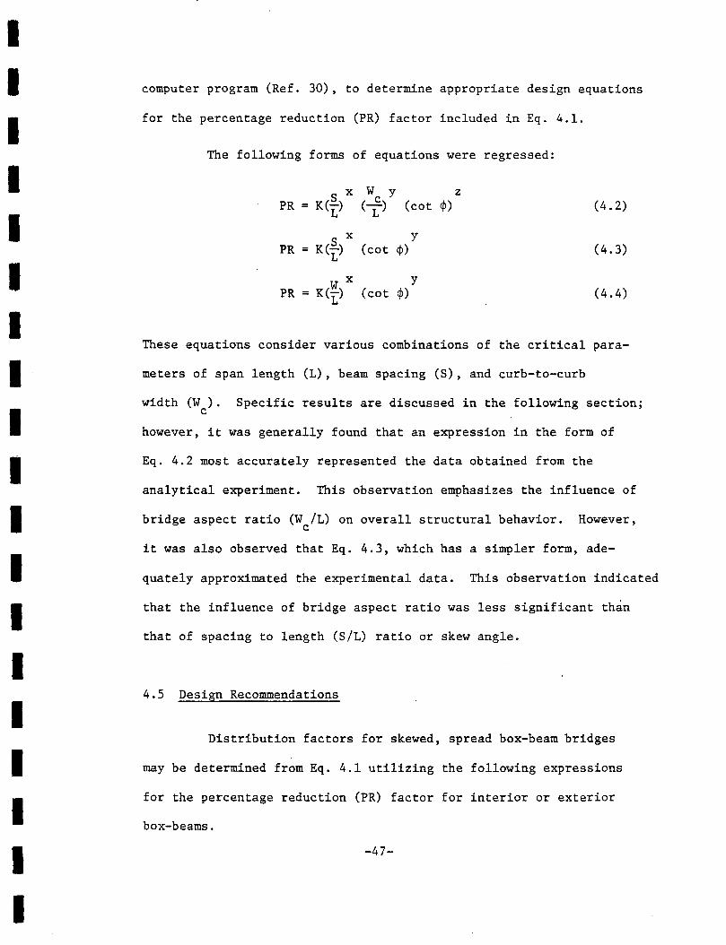
I I I I I I I I I I I I I I I I I I I
computer program (Ref. 30), to determine appropriate design equations
for the percentage reduction (PR) factor included in Eq. 4.1.
The following forms of equations were regressed:
X w y z PR = K(E_) (__£) (cot ¢) (4.2)
L L
X y PR = K(~) (cot ¢) (4.3)
L
X y PR = K(~) (cot ¢) (4. 4) L
These equations consider various combinations of the critical para-
meters of span length (L), beam spacing (S), and curb-to-curb
width (W ). Specific results are discussed in the following section; c
however, it was generally found that an expression in the form of
Eq. 4.2 most accurately represented the data obtained from the
analytical experiment. This observation emphasizes the influence of
bridge aspect ratio (W /L) on overall structural behavior. However, c
it was also observed that Eq. 4.3, which has a simpler form, ade-
quately approximated the experimental data. This observation indicated
that the influence of bridge aspect ratio was less significant than
that of spacing to length (S/L) ratio or skew angle.
4.5 Design Recommendations
Distribution factors for skewed, spread box-beam bridges
may be determined from Eq. 4.1 utilizing the following expressions
for the percentage reduction (PR) factor for interior or exterior
box-beams.
-47-
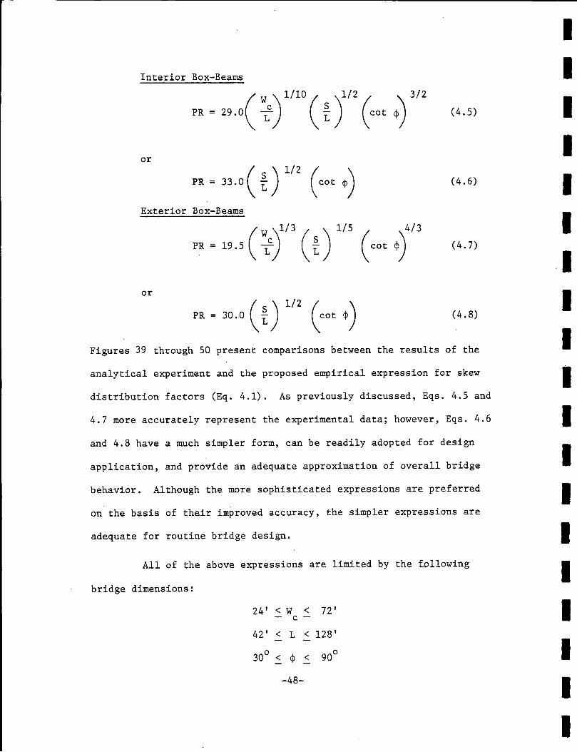
Interior Box-Beams
(
w ) 1/10 1/2 3/2
PR = 29.0 ~ ( t) (coq) (4.5)
or
( s r'2 PR = 33.0 L (cot ~) (4.6)
Exterior Box-Beams
(II )1/3 1/5 PR = 19.5 Lc (f) (cot ¢)
413
(4. 7)
or
PR = 30.0 (t) 112 (cot ¢) (4.8)
Figures 39 through 50 present comparisons between the results of the
analytical experiment and the proposed empirical expression for skew
distribution factors (Eq. 4.1). As previously discussed, Eqs. 4.5 and
4.7 more accurately represent the experimental data; however, Eqs. 4.6
and 4.8 have a much simpler form, can be readily adopted for design
application, and provide an adequate approximation of overall bridge
behavior. Although the more sophisticated expressions are preferred
on the basis of their improved accuracy, the simpler expressions are
adequate for routine bridge design.
All of the above expressions are limited by the following
bridge dimensions:
24 1 < W < 72 I c
42 I < L < 128 I
-48-
I I I I I I
I I I I I I I I I I I I
I I I I I I I I I I I I I I I I I I I
4.6 Suliiiilary
The load distribution behavior of skewed, spread box-beam
bridges under design vehicular loads has been discussed. Load distri-
bution factors were computed for the interior and exterior beams of
bridges constructed with prestressed concrete box-beams. The skew
0 0 0 0 angles investigated were 90 , 60 , 45 , and 30 • The following
observations were made:
1. The load distribution factor decreases with
decreasing angle of skew.
2. The reduction factor is largest at shorter span
lengths for interior beams and at longer span
lengths for exterior beams. This behavior is
primarily the result of increased participation
of the exterior beams in longer spans.
3. The bridge width~to-span ratio, the beam
spacing-to-span ratio, and the skew angle
sufficiently affect the magnitude of the
percentage reduction factor.
Based upon a statistical correlation of bridge parameters with numer-
ical results, simplified equations for computing distribution factors
for interior and exterior box-beams were developed.
-49-

5 . SUMMARY AND RECOMMENDATION
This report describes the development of skew-effect cor
rection factors which are to be applied to the live-load distribution
factors in beam-slab highway bridge superstructures supported by pre
stressed concrete I-beams or box-beams.
Initially, an analytical procedure utilizing the finite
element method was developed to evaluate the response of skewed-
bridge superstructures to design-vehicle loading. The analytical
technique was validated through comparisons with previous field test
results of in-service bridges and by comparisons with alternate anal
ytical solutions. An analytical experiment was then designed for each
type of bridge to study the effects of various parameters on live-load
distribution. A total of 120 I-beam and 72 box-beam superstructures
were analyzed under numerous loading conditions. The results of these
analyses provided a data base which was utilized to develop appropriate
design equations for both interior and exterior beams. The design
equations were based upon formulating appropriate corrections to the
distribution factors for similar right bridges to account for skew,
and yielded the live-load distribution factors required for the_design
of skewed bridge superstructures.
Based upon the results of this study, it is recommended that
the expressions governing live-load distribution in skewed beam-slab
bridges, as presented in Sections 3.5 and 4.5 of this report, be
-50-
I I I I I I I I I I I I I I I I I I I

I I I I I I I I I I I I I I I I I I I
adopted as modifications to the specification provisions currently
governing live-load distribution in right beam-slab bridges. The
proposed expressions are relatively simple in form and clearly yield
values which accurately represent the behavior of skewed beam-slab
bridges.
-51-

6. ACKNOWLEDGMENTS
This study was conducted in the Department of Civil Engine
ering and Fritz Engineering Laboratory, under the auspices of the
Lehigh University Office of Research, as a part of the research
investigation entitled "Development and Refinement of Load Distri
bution Provisions for Prestressed Concrete Beam-Slab Bridges" spon
sored by the Pennsylvania Department of Transportation; the U. S.
Department of Transportation, Federal Highway Administration; and
the Reinforced Concrete Research Council.
The basic research planning and administrative coordination
in this investigation were in cooperation with the following in
dividuals representing the Pennsylvania Department of Transportation:
B. F. Kotalik, Chief Bridge Engineer; H. P. Koretzky, and Hans
Streibel, all from the Bridge Division; and Istvan Januaschek,
Research Coordinator; from the Office of Research and Special
Studies.
The following members of the staff at Lehigh University
made significant contributions: Bert Hoffman in the programming
and execution of some of the. computer analysis, and Charles R.
Kubic in the assembly of material and the writing of this
report.
I I I I I I I I I I I I I I I I I I I
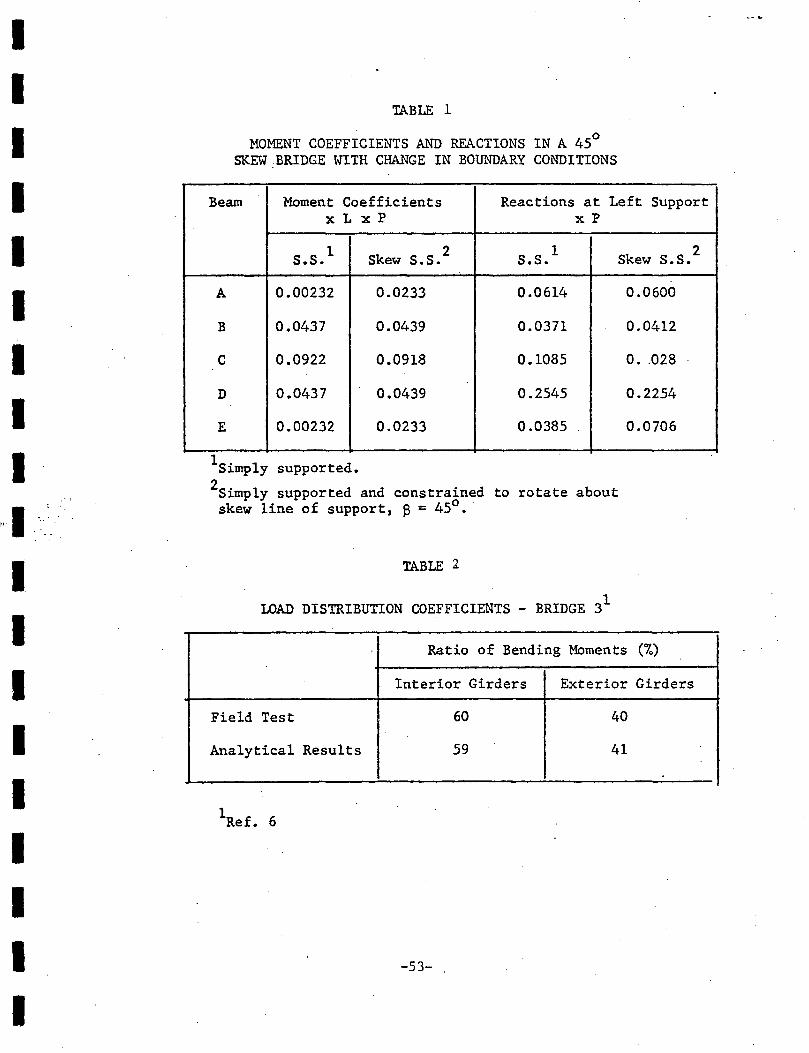
I I I I I I I I I
t•-1 ..
I I I I I I I I I
TABLE 1
MOMENT COEFFICIENTS AND REACTIONS IN A 45° SKEW BRIDGE WITH CHANGE IN BOUNDARY CONDITIONS
Beam Moment Coefficients Reactions at Left Support XL X P xP
s.s. 1 Skew S.S. 2 s.s. 1
A 0.00232 0.0233 0.0614
B 0.0437 0.0439 0. 0371
c 0.0922 0.0918 0.1085
D 0.0437 0.0439 0.2545
E 0.00232 0.0233 0.0385
1simply supported. 2simply supported and constrained to rotate about
skew line of support, ~ = 45°.
TABLE 1
LOAD DISTRIBUTION COEFFICIENTS - BRIDGE 31
Skew S.S.
0.0600
0.0412
0 •. 028
0.2254
0.0706
Ratio of Bending MOments (%)
2
Interior Girders Exterior Girders
Field Test 60 40
Analytical Results 59 41
1 Ref. 6
-53-

Bridge
Field Test
(Ref. 24)
2B Finite Element
(composite)
Finite Element
(non-composite)
Field Test
(Ref. 24)
3B Finite Element
(composite)
Finite Element
(non-composite~
-. ·~--~--- .. ·~·····-
TABLE 3
MOMENT PERCENTAGES •
I: Beam Moment Beam Moment/I: Beam Moment
Truck Moment Interior Center Exterior
89.30 34.0 32.0 34.0
93.57 32.6 34.0 33.2
92.13 33.2 33.8 33.0
92.10 33.8 .33.4 29.2
94.50 32.7 34.3 33.0
83.95 33.2 33.8 33.0
-154-
I I I I I I I I I I I I I I I I I I I

I I
TABLE 4
I LIST OF BRIDGES ANALYZED
Bridge Number
I No. Width of Beams Spacing Length Beam Size S/L ~ft.2 ~in.2 ~ft.2
1 24.00 6 57.60 120.00 AASHO-VI .0400
I 2 24.00 6 57.60 72.00 24/42 .0667
3 24.00 6 57.60 38.40 20/30 .1250
I 4 24.00 5 72.00 120.00 .AASHO-VI .0500
5 24.00 5 72.00 60.00 20/39 .1000
I 6 24.00 5 72.00 42.00 20/30 .1429
7 . 24.00 4 96.00 120.00 AASHO-VI .0667
I 8 24.00 4 96.00 64.00 24/45 .1250
9 24.00 4 96.00 40.00 20/30 .2000
I 10 48.00 11 57.60 120.00 AASHO-VI .0400
11 48.00 11 57.60 84.00 24/48 .0571
12 48.00 11 57.60 48.00 20/30 .1000
I 13 48.00 9 72.00 105.00 28/63 .0571
14 48.00 9 72.00 60.00 20/39 .1000
I 15 48.00 . 9 72.00 42.00 20/30 .1429
16 48.00 6 115.20 96.00 AASHO-VI .1000
I 17 48.00 6 115.20 57.60 24/45 .1667
18 48.00 6 115.20 48.00 20/33 .2000
I 19 72.00 16 57.60 120.00 ASSHO-VI .0400
20 72.00 16 57.60 57.60 20/36 .0833
I 21 72.00 16 57.60 38.40 AASHO-I .1250
22 72.00 14 66.50 110.80 AASHO-VI .0500
23 72.00 14 66.50 66.50 24/42 .0833
I 24 72.00 14 66.50 38.80 AASHO-I .1429
25 72.00 12 78.50 114.50 AASHO-VI .0571
I 26 72.00 12 78.50 65.50 24/42 .1000
27 72.00 12 78.50 39.30 20/30 .1667
I 28 72.00 9 108.00 108.00 AASHO-VI .0833
29 72.00 9 108.00 54.00 24/42 .1667
I 30 72.00 9 108.00 45.00 24/36 .2000
-55-
I

I 'IABLE 5 · I
MAXIMUM DISTRIBUTION FACTORS - INTERIOR BEAMS
I Bridge NUMBER OF LOADED lANES AND SKEW ANGLE No. ~ . '**!:ILL ~ NLL _6.<t. m..L ~ NLL ~
1 2 2 .81 2 • 79 2 .77 2 .71 I 2 2 2 .84 2 .81 2 • 77 2 .66 .
3 2 2 .96 2 .94 2 .93 2 .86 I 4 2 2 .96 2 .92 2 .88 2 .82
5 2 2 1.05 2 .99 2 .92 2 • 78 I 6 2 2 1.17 2 1.07 2 .95 2 .76
7 2 2 1.23 2 1.20 2 1.18 2 1.08
I 8 2 2 1.30 2 1.24 2 1.17 2 .99
9 2 2 1.32 2 1.23 2 1.14 2 .88
I 10 4 4 .94 4 .91 4 .87 4 • 79
11 4 4 .94 4 .90 4 ~87 4 • 75
12 4 2 1.03 3 .98 3 .94 3 .87 I 13 4 4 1.17 4 1.13 4 1.09 4 .97
14 4 4 1.20 4 1.14 4 1.08 4 .89 I 15 4 4 1.24 3 1.13 3 1.07 3 .83
16 4 4 1.84 4 1. 79 4 1.74 4 1.59 I 17 4 4 1.83 4 1.·77 4 1.70 4 1.45
18 4 4 1.86 4 1.72 4 1.58 3 1.24 I 19 6 5 .94 5 .92 5 .90 5 .84
20 6 4 .95 4 .91 4 .87 5 • 75
I 21 6 4 .97 4 .91 4 .96 5 .72
22 6 5 1.07 5 1.05 5 1.04 5 .98
23 6 4 1.07 4 1.04 4 1.01 5 .89 I 24 6 4 1.09 4 1.02 5 .96 5 • 77
25 6 5 1.23 5 1.21 5 1.19 5 1.11 I 26 6 4 1.24 5 1.20 5 1.16 5 1.03
27 6 4 1.30 4 1.21 5 1.12 5 .89 I 28 6 5 1. 72 5 1.68 5 1.65 6 1.51
29 6 4 1.74 5 1.68 5 1.61 5 1.33 I 30 6 4 l. 77 5 1.68 5 1. 60 5 1.23
Number of Lanes I **Number of Loaded Lanes -56-
I

I I TABLE 6
I MAXIMUM DISTRIBUTION FACTORS ~ EXTERIOR BEAMS
~ Bridge NUMBER OF LOADED lANES AND SKE\-7 ANGLE No. *NL '"**NLL 90° NLL 60° NLL 45° NLL 30°
I 1 2 2 .69 2 • 70 2 • 70 2 .72
2 3 2 .67 2 • 67 2 .67 2 .64
I 3 2 2 .56 1 .57 1 .57 2 .58
4 2 2 .80 2 .81 2 .82 2 .83
I 5 2 2 • 75 2 .77 2 .78 2 .73
6 2 2 .73 2 .73 2 .72 2 .62
I 7 2 2 1.01 2 1.02 2 1.02 2 1.01
8 2 2 .95 2 .95 2 .94 2 .88
9 2 2 .87 2 .87 2 .86 2 ~74
I 10 4 2 .71 2 .72 2 .73 3 .73
11 4 4 .68 2 • 68 2 • 68 4 .65
I 12 4 1 • 62 1 .• 61 1 .61 2 .59
13 4 2 .83 2 .83 2 .84 4 .83
I 14 4 2 • 78 2 .76 2 .76 4 0 70
15 4 2 .72 2 .74 4 .71 4 .62
I 16 4 2 1.10 2 1.10 2 1.11 4 1.09
17 4 2 1.02 2 1.01 2 1.00 4 .92
I 18 4 2 1.08 2 1.03 4 .99 4 .85
19 6 2 f> 70 2 .71 2 .72 3 .72
I 20 6 6 .65 2 .64 2 • 63 2 .58
21 6 1 .61 1 .60 2 • 60 2 .53
22 6 2 .78 2 • 78 2 .79 2" 0 78
I 23 6 2 0 74 2 .72 2 .73 2 ~67
24 6 1 .68 2 .·66 2 .67 6 .58. I. 25 6 2 .88 2 .89 2 .91 3 .91
26 6 2 .83 2 .85 2 .86 6 .so
I 27 6 1 .74 2 .75 2 .75 2 .63
28 6 2 1.09 2 1.10 2 1.11 3 1.09
.I 29 6 2 .97 2 .96 2 .• 95 6 .86
30" 6 2 . .• 95 •. 2 .93 2 .91 6 .80
I Number of Lanes **Number of Loaded Lanes
-57-
II

TABLE 7
BROOKVILLE BRIDGE COMPARISON
Percentage of Total Moment Taken by Each Girder (Fig. 38)
Girder
Method
Field Test
Model
A B c
44% 31% 15%
47% 32% 14%
TABLE 8
MOTARJEMI COMPARISON
D
10%
7%
Load Distribution Factors as Reported by Motarjemi and by
Model Analysis
S/L Motarjemi Model
1/4 1.08 1.16
1/5 1.12 1.20
1/6 1.13 1.21
1/8 1.15 1.23
1/10 1.15 1.24
-58-
I I I -1
I I I I I I I I I I I I I I I
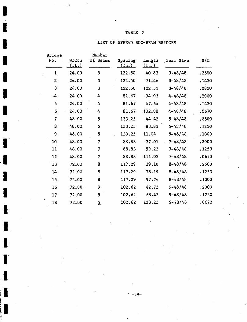
I I TABLE 9
I LIST OF SPREAD BOX-B~ BRIDGES
I Bridge Number
No. Width of Beams Spacing Length Beam Size S/L ~ft.2 ~in.} ~ft. 2
I 1 24.00 3 122.50 40.83 3-48/48 .2500
2 24.00 3 122.50 71.46 3-48/48 .1430
I 3 24.00 3 122.50 122.50 3-48/48 .0830
4 24.00 4 81.67 34.03 4-48/48 .2000
5 24.00 4 81.67 47.64 4-48/48 .1430
I 6 24.00 4 81.67 102.08 4-48/48 .0670
7 48.00 5 133.25 44.42 5-48/48 .2500
I 8 48.00 5 133.25 88.83 5-48/48 .1250
9 48.00 s 133.25 11.04 5-48/48 .1000
I 10 48.00 7 88.83 37.01 7-48/48 .2000
11 48.00 7 88.83 59.22 7-48/48 .1250
ll 12 48.00 7 88.83 111.03 7-48/48 .0670
13 72.00 8 117.29 39.10 8-48/48 .2500
I 14 72.00 8 117.29 78.19 8-48/48 .1250
15 72.00 8 117.29 97.74 8-48/48 .1000
I 16 72.00 9 102.62 42.75 9-48/48 .2000
17 72.00 9 102.62 68.42 9-48/48 .1250
18
I 72.00 9_ 102.62 128.25 9-48/48 .0670
I I I.
I I -59-
I

I I
TABLE 10
MAXIMUM DISTRIBUTION FACTOR - INTERIOR BEAMS I Bridge 90° 60° 45° 30°
I Number
1 1. 73 1.62 1.45 1.12 I 2 1.63 1.56 1.46 1. 22 I 3 1.51 1.47 1.40 1.23
4 1.17 1.07 0.96 0.79 I 5 1.13 1.07 0.98 0.80
I 6 1.07 1.04 0.99 0.86
7 1.92 1.82 1.66 1.32 I 8 1.87 1.80 1.69 1.42
I 9 1.85 1. 79 1.69 1.43
10 1.39 1.27 1.12 0.86 I 11 1.32 1.25 1.16 0.95
12 1.27 1.22 1.16 0.98 I 13 1.72 1.61 ' 1.46 1.18 I 14 1.67 1.60 1.51 1.25
15 1.66 1.61 1.52 1.27 I 16 1.55 1.46 . 1. 33 1.04 I 17 1.51 1.44 1.35 1.12
18 1.47 1.42 1.35 1.14 I I
-60- I I

I I
TABLE 11
I MAXIMUM DISTRIBUTION FACTOR - EXTERIOR BEAMS
I Bridge 90° 60° 45° 30° NL Number NLL DF NLL DF NLL DF NLL DF
I 1 2 2 1.30 2 1.21 2 1.12 2 0.93
I 2 2 2 1. 34 2 1.28 2 1. 22 2 1.08
3 2 2 1. 36 2 1. 32 2 1.27 2 1.16
I 4 2 2 1.01 2 0.94 2 0.87 2 0.72
I 5 2 2 1.03 2 0.98 2 0.91 2 0.79
6 2 2 1.05 2 1.02 2 0.99 2 0.90
I 7 4 3 1.45 3 1.34 3 1.22 4 1.01
I 8 4 3 1.48 4 1.40 4 1. 34 4 1.17
9 4 3 1.50 4 1.43 4 1.37 4 1.21
I 10 4 3 1.09 3 1.01 3 0.91 4 0.75
11 4 3 1.13 3 1.05 4 0.98 4 0.85
I 12 4 3 1.15 4 1.09 4 1.05 4 0.93
I 13 6 4 1.32 4 1.·22 4 1.11 4 0.92
14 6 4 1.39 4 1.31 5 1. 22 5 1.05
I 15 6 5 1.40 5 1.32 5 1.24 5 1.08
I 16 6 4 1.22 4 1.13 4 1.03 4 0.86
17 6 4 1. 26 4 1.19 5 1.10 5 0.95
I 18 6 5 1.29 5 1.22 5 1.15 5 1.00
I I -61-
I I

I I
TABLE 12
I MAXIMUM PERCENTAGE REDUCTION - INTERIOR BEAMS
Bridge I Number 90° 60° 45° 30°
1 0.00 6.36 16.18 35.26 I 2 4.29 10.43 25.15 I 3 2.65 7.28 18.54
4 8.55 17.95 32.48 I 5 5.31 13.27 29.20 I 6 2.80 7.48 19.63
7 5.21 13.54 31.25 I 8 3.74 9.63 24.06 I 9 3.24 8.65 22.70
10 8.63 19.42 38.13 I 11 5.30 12.12 28.03 I 12 3.94 8.66 22.83
13 6.40 15.12 31.40 I 14 4.19 9.58 25.15
I 15 3.01 8.43 23.49
16 5.81 14.20 32.90 I 17 4.64 10.60 25.83
I 18 0.00 3.40 8.16 22.45
I -62- I
I
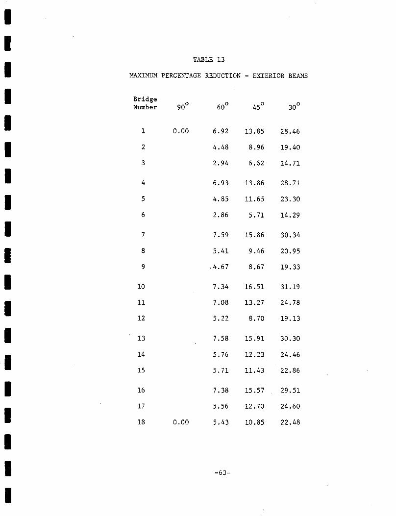
I I
TABLE 13
I MAXIMUM PERCENTAGE REDUCTION - EXTERIOR BEAMS
I Bridge 90° 60° 45° 30° Number
I 1 0.00 6.92 13.85 28.46
I 2 4.48 8.96 19.40
3 2.94 6.62 14.71
I 4 6.93 13.86 28.71
I 5 4.85 11.65 23.30
6 2.86 5. 71 14.29
I 7 7.59 15.86 30.34
I 8 5.41 9.46 20.95
9 .4.67 8.67 19.33
I 10 7.34 16.51 31.19
I 11 7.08 13.27 24.78
12 5.22 8.70 19.13
I 13 7.58 15.91 30.30
I 14 5.76 12.23 24.46
15 5. 71 11.43 22.86
I 16 7.38 15.57 29.51
I 17 5.56 12.70 24.60
18 0.00 5.43 10.85 22.48
I I -63-
I

I 0"1 .p.
• I
A
~ D.
A
. ,.
8 c D E
(a) Prestressed Concrete !•beam Bridge
rfl D D D D '
8 c D E
(b) Prestressed Concrete Spread Box-Beam Bridge .•
Fig. 1 Besm-Slab Bridge Cross Section
-------------------

I I I I I I I I I I I I I I I I I I I
~---------- ~----------
I -----------t------------------.--1---------- w
I 5
·----~----t-----~---Js ~---- ---- t- --------- _ __._
1- ~ -1 o Right Bridge
Skewct
I
-------~---------------- -------
. .
w
L _,
b Skew Bridge . '
w
~ ~ 2.S -~. ~ 1- s .. ,. s I s -1- s . I
c Section
Fig. 2 Plan and Cross Section of a Beam-Slab Bridge
-,65-

··~
0 I·
14' (min) • I 141
. I ~ ~ --EZm-
~~ ~ ~
~ ~ -~ ~ ~
~ l ·~ Axle Loads: 32 k 32k 8k
HS 20-44 Design Load Vehicle
0 I·
20.41
·1- 13.01
. ~i ~ ~
~-wJ -qr~ - -'i'I~. - 10 C\1 I I r-..: ¢~ 1'- lO . w . fQ5229.
RXXSJ. EX&":3 EXZ9 .
l t l Axle Loads= 32.5k 32.3k 10.3 k
Test. Vehicle
Fig. 3 Vehicular Loadings
I I I I I I I I I I I I I I I I I I I

------... ..... ...
• ... .. .. ... ... ... ..
. I
I
. I
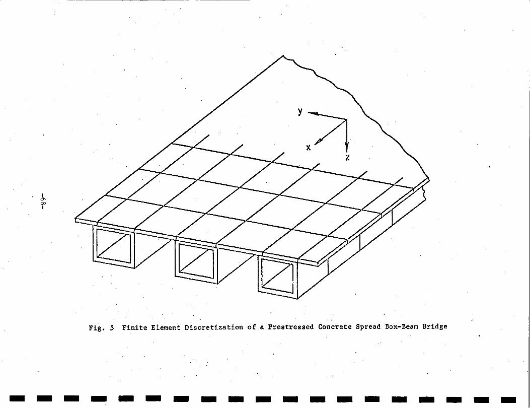
I 0\ 00 I
Fig. 5 Finite Element Discretization of a Prestressed Concrete Spread Box-Beam Bridge
-------------------

. - - - - - - - - - - - -· - - - - - - -
I ()\
-o I s
s
s
s
s 8 ~
S r c -1- li---+--+---+--Q---t---t---t---tl
s D -+- k----+--r--+--Q---t---t----t---1!
s • E _.__ 4---L--...1---"---o---"----"--....._---r
b
Support Line L ·--------------~~ Support Line
o Location Of Max. Beam Moment Response
30° Support Line
b
Support Line
Fig. 6 Location of the Maximum Beam Moment Response in a ~0° Skew Bridge (Right Bridge) and a 30° Skew Bridge - Concentrated Load at Midspan of Beam C

A s
B s
c ·s
D s
E Support Line .
I A -...j
0 I
B
c
0
E
Fig. 7
b
\--~-__.).....__..l-_-tr--~-~--.-.--,,_,~-Support Line
o Location Of Max. Beam Moment Response
0 Location of the Maximum Beam Moment Response in a 60° Skew Bridge and a 45 Skew Bridge - Concentrated Load at Midspan of Beam C
- - - - - - - - - - - - - - ·- - - - -

I I I II-
I I I I I I I -1.
I ~--
1 I I I
0.12
O.t I t= 0.1
0.1 0-~~-~-~-=-=-;...::-::...::.:-s:.::..::_ 1- • -.....
'· '· (/) 0.09 .... .z
·' w 0.08 ·o -u.. u.. w 0 0
0.07
0.06
...... """'¢-. ·--..... z 0.05 -=-=-~<~. ::~:::--~-P':I .. ~-==-==-~ .... ~--
·-c...... ·-........
w I . o---...._. - ....... _,. ~ 0.04 ·"'--·~ ~---~ .
·0.03
0.02
0.01
90
·---·--.., --. _,...,____ . ,_,_. . - . --o- . ..-. .
75 60 45 SKEW AN~LE, degrees
c Finite Element (Analysis)
A Finite Element (Ref. 23.)
0 Finite Difference (Ref. 40)
Beam C
Beam 8-
Beam A
30
Fig. 8 · MOment Coefficients in a 5-Beam Br~dge Neglecting the Eccentricity of the Beams to the Slab
-71-.

0.12
0.11
---a.--
0.1 Oqr------..;..--~
. (J) 0.09 1-
fti 0.08 -(.) -tt 0.07 .... w ··o (.) 0.06
Lr-"-_
--~ 0.05 ·~-------5---w ~·0.04 ~·
0.03
0.02
0.01
90
0
---75
.o- - .-o---60 45
SKEW ANGLE, degrees
~ .- 0.1
e GKT = 0. e~=O.· EI
30
~ = 0.5 GKT
= 0.035 EI . D
Beam C
Beam 8
Beam A
Fig •. 9 Homent Coefficients in a 5-Beam Bridge Including the Beam Eccentricity·and Torsional Rigidity
-72-
I I I I I I I I I I I I I I I I. I I I

I I I I I I I I I I I I I I I I I I I
e Load Points
Fig. 10
25.0 '
50.0
j s'-10 .. js'-I011,j,s'-lo" J
Static Load Test of Bridge 3 (Ref. 6)
-73-
-f'-C\1

I ....... .p.. I
...,,_
·..:-
0
-f-
L-
1-
• $lora ol s• Clro.
\ Interior Beom - -\.
" Center Beam - -1\ \ Exterior Beam - -"' 12 <.&> 4'- 2 11
= 501 -0 11
Plan and Discretization
ez• t zo:r e.!."
I
L.A
Fig. 11 AASHO Test Bridge (Ref. 24)
-I
-~f.
0 -· I{)
- =o -0 I
-· I{) I{)
Beam Properties
Beam Ix (In 4 > Bridge Size w /Coverplate
2B wl8 x50 1040 JB wl8x60 1176
-------------------

--- -- - ... -- -·---------
I -.I V1 I
~
1.00 r- -ro--o
f-- ~
- - r--
0:: 0.75 f2 (.)
- - ---
~ 2 0
0.50 ._ :J en cr ._ (J)
0 0.25
C1) C1) C1) C1)
C1) C1) - - - - -- (/) ·- .~ ~ ·- ·-(/) (/) (/) (/) (/)
0 0 0 0 0 0 0.. 0.. 0.. 0.. 0.. 0.. C1) C1) E C1)
.~ E - C1) E ·Q) E G> E - E - - -0 ·- 0 (/)
(.) (/) (.)
·u; 0 (/) 0 (/) 0 (/) 0 0 0 0 (.) 0 (.) 0 (.) 0 (.) 0.. I 0.. I 0.. I 0.. I 0. I 0. I
E c E c E c E c E c E c - c 0 0 0 0 c 0 0 0 0 c 0 0 0 0
.Q'l (.) z u z 0' u z (.) z· .Q' (.) 2 (.) z
(/) en en en en (/) en en en en (/) en m m en Q) Q) Q)
0 C\J C\J t() r<> 0 C\J C\J t() t() 0 C\J C\J t() t()
INTERIOR CENTER EXTERIOR
Fig. 12 Distribution Factors for Interior, Center and Exterior Br~dge Beams -AASHO Test Bridge
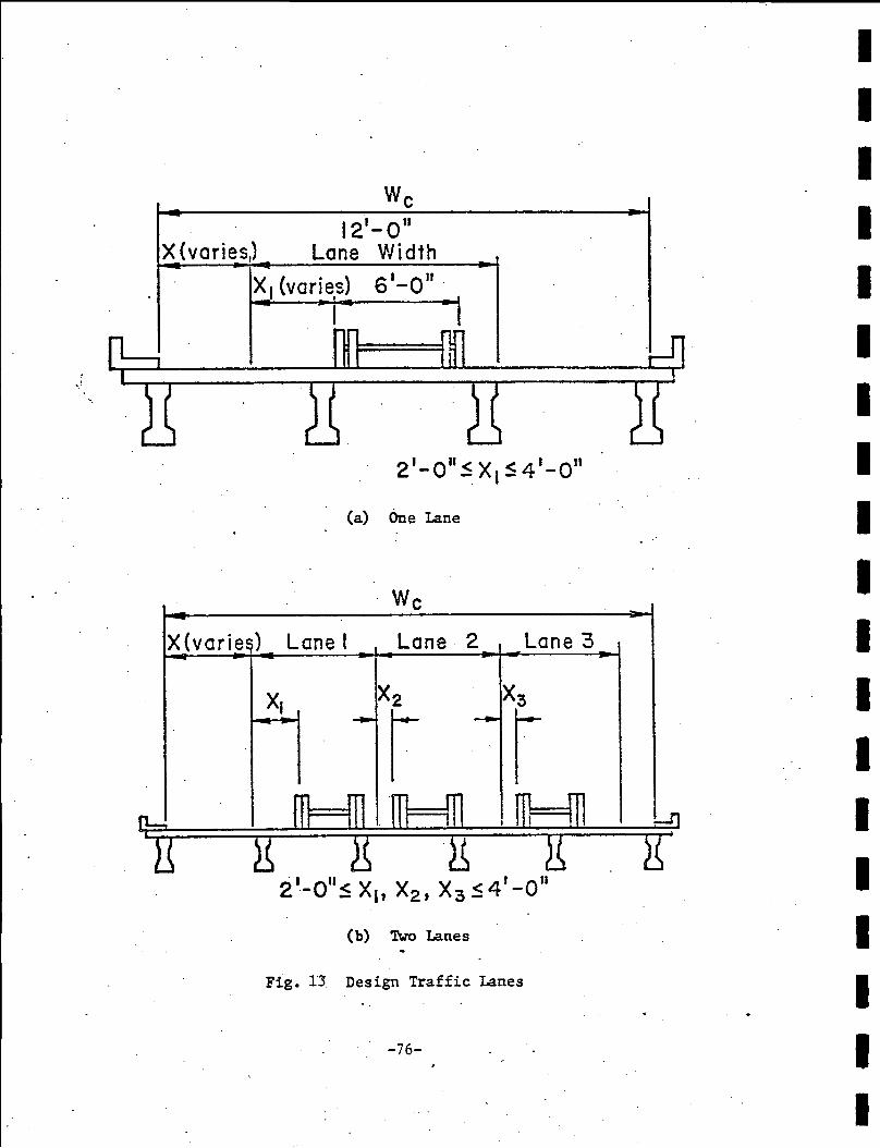
•.
X (varies,) 121
- Q II Lane V/idth
X1 (varie,s) 6'-o" ·
2'-o" ~- x1 s 4'-o"
(a) One Lane
X(varied Lane I Lane 2 Lane 3
x, x2 x3 - r - r I I
(b) Two Lanes 4
Fig. 13. Design Traffic Lanes
-76-
I I I I I I I I I I I I I I I I I I I

I I I I I I I I I I I I I I I I I I I
A
A
8
c D
E
~
L/2
l:
--1 t--d/2 : 9 i I • I
I 9 l I l I I T ! I I l t n I ~ I : I I
'ct. L
1-o. Truck· Centroid Positions
L
• Location of Maximum Moment, Beam A
5/L=O.I
<P = 90°
5/L =0.1 <P = 45 °
.. I
-I
Fig. 14 Load Positions and Locations of Maximum Moment REsponse - Beam A
-77-

A
A
A
8
c D
E
_.... r-- d/2 ! I I C) ! I I
I l
I I I
I "'{ I I j I I I I I I I
> I
I I
i L/2 L
(typi eel)
(typical)
L. o Truck Centroid Posit ions
L
S/L=O.I cf> = 90°
...t • Location of Maximum Moment, Beam 8
Fig. 15 Load Positions and Location of Maximum Moment Response - Beam B
-78-
I I I I I I I I I I I I I I I I I I I

I I I I I I I I I I t
I I I I I I I I I
A
A
A
8
c D
E
-- r-:- d/2 I I I C) I I • I
I T I ¢ : I I I I > I I I
L/2 ~ ~~-----------~-- ~
',' ,'b.', ,, ' '
L
l: L/2 -1 i
o Truck Centroid Positions
L
S/L=O.I </> = 90°
S/L=O.I </> = 45°
S/L=O.I </> = 30°
L _, • Location of Maximum Moment, Beam C
Fig. 16 toad Positions and Location of Maximum Moment Response - Beam C
-79-
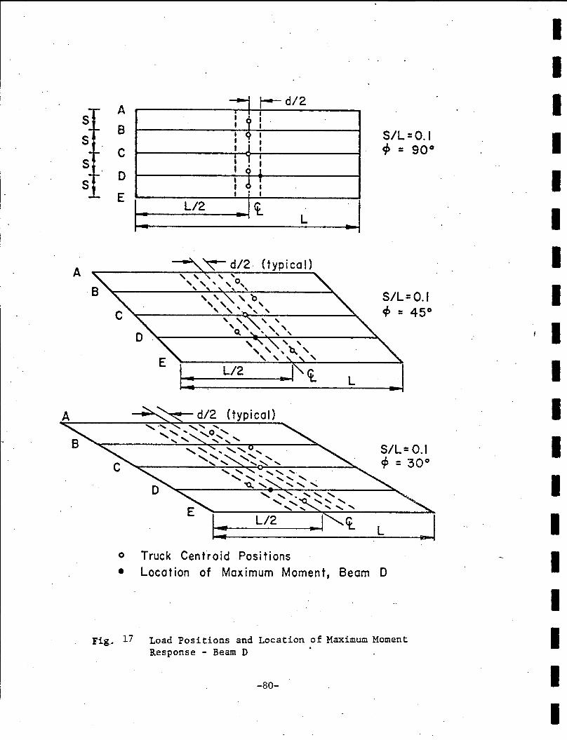
A
A
8
c D
E
0
• Truck
~ t--d/2 I y : I I
I <? I I • I I j I
! 1 I
I o l ' ~ l I I I ' I
L/2 -~ft.
' ' ' 'b ' ' ' ' ' ' ', '
L
1~:~-----. _L/_2 _ __,_-..~I <t
l: Centroid Positions
Location of Maximum Moment,
L
<t
Beam
S/L=O.I 4> = 90°
S/L=O.I 4> = 45°
... I
S/L= 0.1 cp = 30°
L
D
Fig. 17 Load Positions and Location of Maximum Moment Response - Beam D
-80-
I I I I I I I I I I I I I I I I I I I

I I I I I I I I I I I I I I I I I I I
A
A
A
8
c D
E
0
•
Fig. 18
-.-: r----d/2 I I I < I I ' I
I y I I I I I I I I I I I I
I • I
f > ! L/2 i L
L/2
L/2
Truck Centroid Positions
L
S/L =0.1 ~ =90°
S/L=O.I tp = 45°
.. I
Location of Maximum Moment, Beam E
Load Positions and Location of Maximum Moment Response - Beam E
-81-
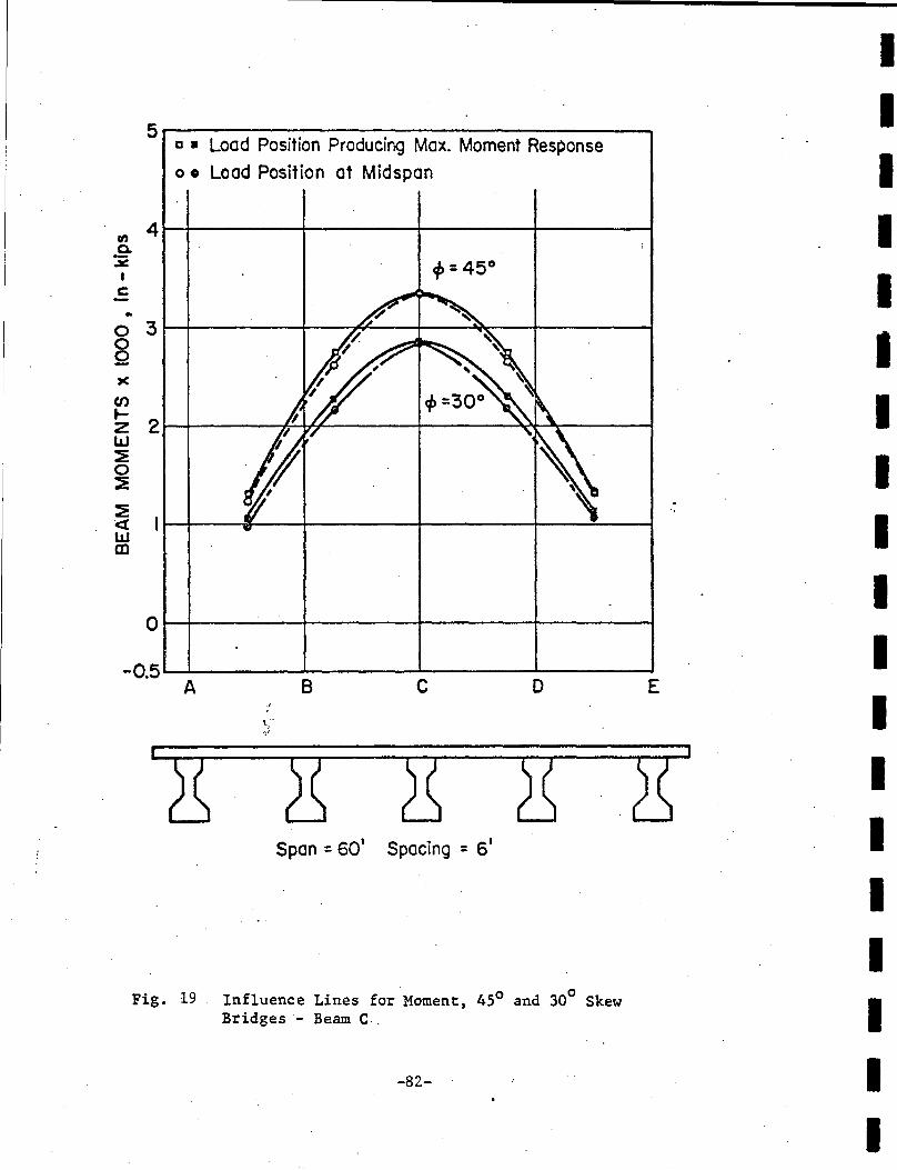
5~------------------------------------~ a • Load Position Producing Max. Moment Response
en 4 ~ :;: I c: ..
o • Load Position at Midspan
0 3~~-------4--~~---+--~~---r------~
8 )(
(/)
~ 2~~------~~------~--------~~------~ w ~ 0 ~
~ <C w Ol
0~~-------+--------~--------~-------;
-Q5~A~------~B------~C--------D~----~E
Span = 60' Spacing = 6'
Fig. 19 Influence Lines for Moment, 45° and 30° Skew Bridges - Beam C-.
-82-
. .,
I I I I I I I I I I I I I I I I I I I
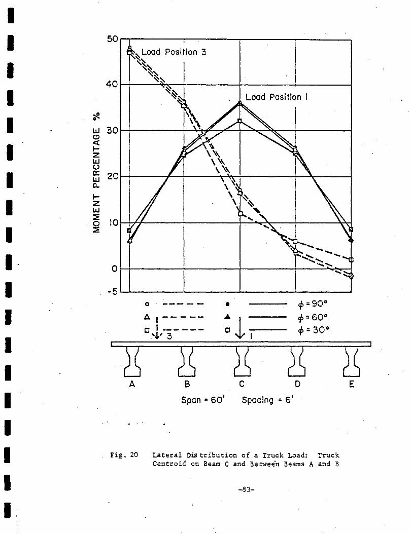
I I I I I
~ 0
w (,!)
I <( t-z LLJ (.)
I et: w 0..
t-
I z LLJ ~ 0
I :E
I I I I I I I I I I
50~--------~~----~--------~------~ ~Load Position 3 ~~ ~~ ~~ ~~
40~----~~~--------+---------~------~
Load Position I
0
-5 0 ----- • cp = 90°
A ,------ :l 4> = 60° c I------ 4> = 30°
'"'' 3 g 8 g 8 A B c D
Span= so• Spacing = s· .
Fig. 20 Lateral Distribution of a Truck Load: Truck Centroid on Beam C and Between Beams A and B
-83-
g E
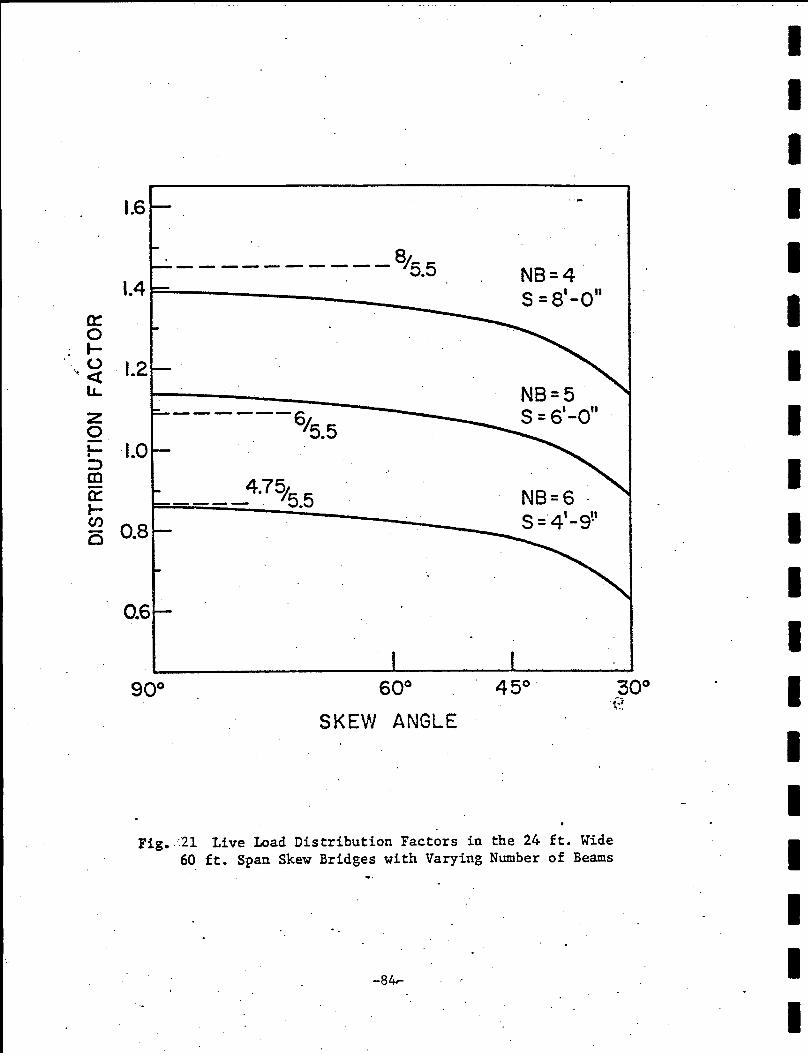
1.6
0.6
. a, ---------- '5.5
4.75/i ---- . 5.5
60°
SKE'wV ANGLE
N8=4· S =8'-on
NB=5 s = 6'-o"
NB=6 -s =·4'-9!'
Fig •. :21 Live toad Distribution Factors in the 24 ft. Wide 60 ft. Span Skew Bridges with Varying Number of Beams
-84--
I I I I I I I I I I I I I I I I I I I

I I I I I I I I I
,,I I I I I I I I I :.1.
0:: 0 t-(.)
<t ·-., lL.
z 0 t-:J CD 0:: t-(J)
0
0 <t g
I I I I I A 8 c 8 .A
30 30' span 60 60'
120 120'
C-60 - __:;5.5_ --- - - .- -- -8-60
8-120 A-120
A-60
A-30
60° 45°
SKEW ANGLE
Fig. 22 Live Load Distribution Factors in the 24 ft. Wide Skew Bridges, 5 Beams with Varying Span Length.
-85-

I -
1.8
0::: 0 1.6 ..... (.)
<t LL
z 0 -..... :::> al a:: ..... C/)
0 0 <t g
120'
S/5.5
SPAN'· L
60' 30'
~~~~=~~IWc 1- L .I
~2 lf1o V9 If a lf1. Vs
S/L
Wc=24'
N8=5
2 Lanes s =6'
Fig. 23 Live Load Distribution Factors in the 24 ft. Wide Skew Bridge with 5 Beams
-86-
I I I I I I I I I I .I
I I I I I I I I
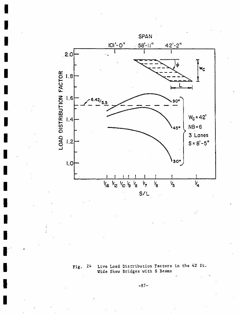
I I I I I I I I I I I I I I I 1.·
I I I
SPAN
101'- o" . 58'-11" 42'·2"
~}c
~6 ~12 1110 ~ Ya Y7 S/L
1- L .. 1
Wc=42'
45° NB=6
lt. 5
3 Lanes
s = 81-5 11
Fig. 24 Live Load Distribution Factors in the 42 ft. Wide Skew Bridges with 6 Beams
-87-

1.60 • 90° {Right Bridge) o 60° Skew Bridge. We= 24ft.
1.50 o 45 ° Skew Bridge A 30° Skew Bridge
1.40 0:: 0 ...,_ 1.30 u tt 1.20 z NB=4 0 1.10 s =a·= o" 1-
I ::::> 00 m 1.00 00 I a:: NB=6 1- 5=4"10
11
~ en 0.90 0 NB=5
0.80 S=G'-0"
0.70
0.60 V3o Y2o Yt5 . Ya Y7 '16 v4 y3
; ':.
S;L RATIO.
Fig. 25 Distribution Factors for Interior Beams - 24 ft. Wide Bridges
-------------------

-·-------- ·-·---------!
I CX> 1.0 I
1.80
1.70
1.60 0::
1.50 0 ._ u ~ 1.40
z 1.30 0 ._ 1.20 :::>
m 0::: 1.10 ._ (f)
0 1.0
0.90
0.80
0.70 V3o Y2o Yt5
., '.-•
We= 48ft.
• 90° Right Bridge
c 60° Skew Bridge
o 45° Skew Bridge
A 30° Skew Bridge
NB = 6 s:: 9~7 11
Fig, 26 Distribution Factors for Interior Beams - 48 ft. Wide Bridges

1.80 Wc=72ft.
~ ~ 1.70 tr • go• ( Rloht Bridoe l 0 "()
"'"'"'-0 o 60° Skew Bridoe 1.60 o 45° Skew Brtdoe
a:: 1.50 A 30° Skew Brldoe
~ 1.40 N8=9 (.)
(t s = 9'-0" 1.30 : z ~ 0 .__ 1.20
I ::> N8=12 ~ m 0
S= 6'-7" I ~ .__ en 0
{ N8=14 S= 5'-7"
0.70 Y3o Y2o 1~s Va Y1 Y6
S;L RATIO . Ys .y4 v3
Fig. 27 Distribution Factors for Interior Beams 72 ft. Wide Bridges
-------------------

------~------------
1.20 we= 24ft. o Right Bridge
1.10 o 45° Skew A 30° Skew
a:: 1.00 0 l-() 0.90 ~
I z NB=4 0 0.80 s=a·-o"
I l-
{ } 1.0 :::> I-' ro 0.70 NB=5 I
a:: s = s·-o" l-~ 0.60
NB=G
0.50 S= 4'-1011
0.40 Y3o Y2o ~5 Ya y1 Ys y4 1;
3
S;L RATIO
Fig. 28 Distribution Factors for Exterior Beams - 24 ft. Wide Bridges

I \0 N I
. '
1.10
~ 0 t; 0.90 ll z 0.80 0 1-ffi 0.70 n:: 1-• (f) 0.60 0
\JVc =48ft. • Right Bridge o 45° Skew
A 30° Skew
N8=6 s = 9'-711
OAQL----,L-~1 --1~------~,,~,~~~--~~L-~~~------~~~~----------~ v30 ~Q Yrs 18 11 6 5 4
S;L RATIO
Fig. 29 Distribution Factors for Exterior Beams - 48 ft. Wide Bridges
--------------------

- - - - - - - - - - - - - - - ·- - - -
Wc=72ft.
1.20 • Right Bridge o 45° Skew
0:: 1.10 A30° Skew 0 l-~ 0.90 NB=9 tJ: S = 9•-o" z 0.80 0 l-
{ l NB= 12 :J m 0.70 . s = 6'-7" I 0::
\.0 1- • w NB=I6 I (f) 0.60 NB= 14 0 S= 4 1-10 ..
S=51-7 11
0.50
0.40 . I Ya IJ7 lfs Ys 1;4 Y3o lf2o Y15 S/L RATIO
Fig. 30 Distribution Factors for Exterior Beams - 72 ft. Wide Bridges
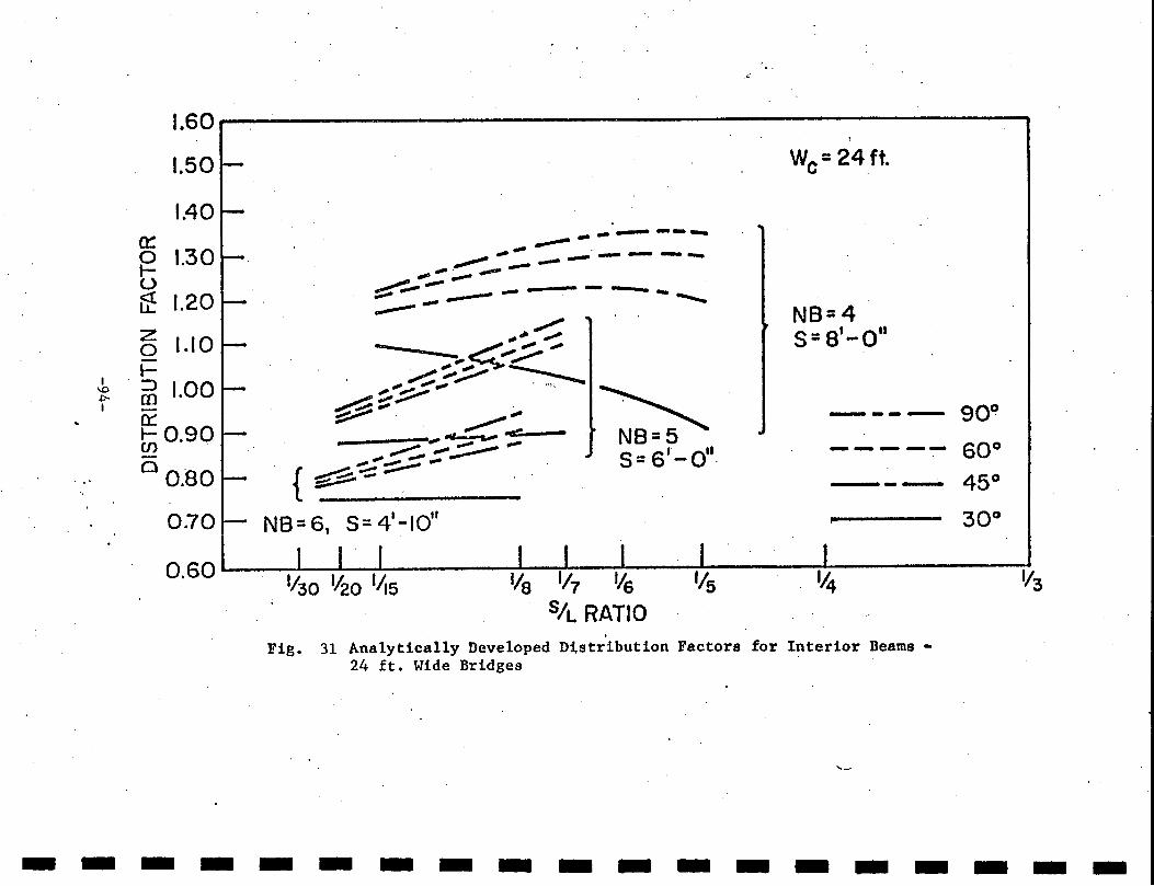
I '-'> -1:'-I
1.60
1.50
1.40 0::
1.30 0 t-u lt 1.20 z 1.10 0 r-:::> 1.00 en 0::: ~0.90 0
0.80
0.70
,.;·
~· s= 6'-o".
NB=6, 5=41-1011
We= 24ft.
NB=4 s=a'-o ..
---- 900.
----- 60°
o.soL----L--L-~------~~~a--~~~--~~~s----~------·~74------------~v3
5/L RATIO Fig. 31 Analytically Developed DLstribution Factors for Interior Beams -
24 ft. Wide Bridges
-------------------

-------------------
1.80
1.70
0:: 1.60 0 ~ 1.50 u
I
ft z 1.40 0 ~ 1.30 :J m
1: 0:: 1.20 1.0 r-VI (/) I 1.10 0
1.00
0.90
0.80
----- ----- ...... ---------------. __
-------- ---. ~- ---~--- -- NB=9 s=6'-o"
·We= 48ft.·
NB=6 s = 9'7"
---- goo
--~---60°
--- 45°
------30°
Fig. 32 Analytically Developed Distribution Factors.- 48 ft. Wide Bridges
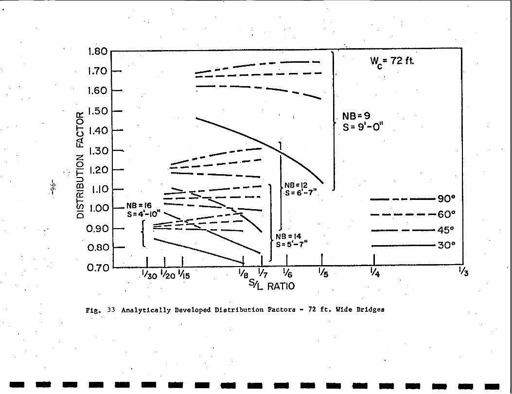
I \.0
"' . I
1.80 -----~-----~--~~-~---:------,
1.70
1.60
a:: 1.50 0 t; 1.40 lt
1.30 z 0
...... 1.20 :J
-------------- .. _.,..,.,.. -------------------.-- ...............
--------~- ' --.-- --· ------------m 1.10 .........,_ ___ ----a:: ::. - .::::::-- - - - -
NB=I2 ·S= 6'-7".
~ NB=I6 --- ~ 0 5=4'-10
11
"""' - ~ f ~ _,.... -::::-:.. - -:""' ~.:~.t l ~I ~~;.:"r.. I 070- I I I lA . .IJ3o lf2o 1/js IJa V7 Is 5
51L RATIO
We= 72ft.
. NB=9 S = g•-on
--- goo
--.~---60°
--- 45° ------30°
Fig. 33 Analytically Developed Distribution Factors - 72 ft. Wide Bridges
- - - - - - - - - - - - - - - - - - -.

I I 1.20 ,
I I 0 ....
<t 1.00
~c =0.20
"' ~ =0.04
__. - -a::
I 0:: ·o
-.. ........:: j
.......:
... I
(.)
~
I I z ... ~
'•, 0 ~ :::>
0.80 "-
to-......
......
' {:c =1.86
1~ -f-=0.20
I co -a: ... 0.60 -
I (J) -0
.I
-
. I I 1 t 0.40 . 90 75 60 45 30
SKEW ANGLE (DEGREES)
I · Interior I.
(IJ ~-
I (/)
U') t)
3:
I (/)
{/) ir
I I I~ L
I Fig. 34 Interior Beam Distribution Factor Ratio
I -97-
I·

• .... ~ "v
0
~ a:= a:= .
. 0 1-u ~ z 0 -1-::> (I)
cr:: 1-(/) -0
1.20,.------------------.
1.00
L = 0.20
0.80
0.60
0:40 90 75 . 60 45 30 SKEW ANGLE (DEGREES)
Exterior
I· L
Fig. 35 Exterior Beams Distribution Factor Ratio
-98-
I I I I I I I I I I I I I I I I I I I

-------------------
I 1.0 1.0 I
Fig. 36 Typical Skewed Spread Box-Beam Bridge Discretization
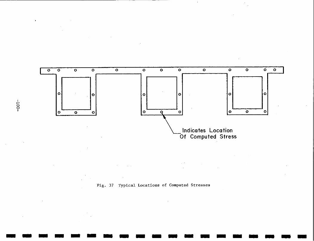
I 1-' 0 0 I
I 0 0
0
0
0 0
0
0 0
0 0 0 0 0 0 0 0 0 I
0 0 0 0
0 q 0 0 0 0
\_Indicates Location Of Computed Stress
Fig. 37 Typical Locations of Computed Stresses
-------------------

- - - - - - -·- - - .. - - - - - - - -
I 1-' 0 1-' I
l'-3"t'-611
~ .. : . /) :;-:~ !';--...........
~·
A
...
1'6" 2'-o"
28' 0" Roadway - - .,1-:'i I Jil 'I 2 3 4 5
I I I I I I I I I 1 f~2· Min. Slab
:~:.: 4' : .~· . ..... , . t . : . ., . •• ~~: :b. ..... : •. : • •• ""'' :~.- .·:..:: .•. • .l>:· • •. A· . ... : : .. .. · ···"":".}~·. ·~
3'1 []. .. t ... ·6~
I~ I~ c D • 1 ' .
Do _.._
~ 4 '• '4
5~· . . . . .... . ...
4'-o'
3Spo. (II) a•-to" =26'- 611 2'-o' '1'-6~' I
Fig. 38 Cross Section of the Brookville BrJdge
Parapet
Curb

2.0
1.8
1.6
--eLL. a - 1.4 0::: 0 ~ u <I: IJ...
z 0 ~ :::J (!)
1.2
0::: 1.0 ~ (f) -a
0.8
0.6
w 11. s 't2 312
P.R. = 29.0 ( Lc) 10
( T) (cot¢)
DF4> = DF90 (1- I~)
• • -~30° --·---- .-- 60° • -- ---.-- ---·- . ·-- --- ---· 45° ---• • • --- -- ----• • •
-- NB=3
--- NB=4
0.4~----~------~------~-------~------~-------~ 0.10 0.20 0.25 0.30 0.15
S/L 0 0.05
Fig. 39 Interior Box-Beam Distribution Factors, W = 24 ft. c
-102-
I I I I I· I I I I I I I I I I I I I I

I I I
2.0
• goo
I ------. 1.8 • • • 60° -I • •
I • -45° l.6
I -~ 1.1...· • I a - 1.4 0: 0 ·- • I t- -- ---u goo ..--- ---- • <t 60° -----· 30° 1.1.. •
I 1.2 45° ----- ---~-----z 0 • • t- •
I ::> 30° --IIl ----0: 1.0 ---t- • --I (f) ---- • a
I • 0.8
I I NB=5
0.6 -~-- NB=7
I I 0.4
0 0.05 0.10 0.15 0.20 0.25 0.30 S/L
I Fig. 40 Interior Box-Beam Distribution Factors, W = 48 ft. c
-103-
I

I 2.0 I
I 1.8 I
• goo I --• •
1.6 • • t -soo I __ ... .t ·-- ----a- . -- I goo•--
LL. ____ ....
0 ·--- 1.4 60°•- ----
a:: 45°.---.- - ... ---- I 0 --. I-(.) • I <l: 30° ...... LL. .......
1.2 ................... • z ....... I 0 • ..._, .......
I- • "'- ....... ::>
...... 30° ......... CD • I -a:: 1.0 I-CJ) I -0
0.8 I I
NB=8 0.6 I ---- NB=9
I 0.4 I 0 0.05 0.10 0.15 0.20 0:25 0.30
S/L Fig. 41 Interior Box-Beam Distribution Factors, W =72 ft. I c
-104-
I


I 2.0 I
goo I 1.8 • • I •
60°
I • • • 1.6 45° I
--&- I LL.. 0 - 1.4 0::: 30° I ~ ·---- •
. ---u goo._.- --· I <t • --LL.. . ---1.2 60° ---
2 45° ·----·--- --
0 I - • ..... ::> 30° --CD --- ..... ---- - ,_, ___
I -0::: 1.0 I- • en • I 0
• 0.8 I
I 0.6 N8=5 I
---- N8=7
I 0.4 I 0 0.05 0.10 0.15 0.20 0.25 0.30 -
S/L I Fig. 43 Simplified Interior Box-Beam Distribution Factors, W = 48 ft.
c
-106- I

I I
2.0
I I 1.8
- --- -- -- ·--. --
I goo
I 1.6 • • • ___ _. 60°
I . _..,.. ----g. --- --goo lL.. • • 0 • - 45°
I 1.4 60° . ------ __ ....., ___ .-a::: 45° • 0
I 1- -u
30° • <t ... __ • lL.
1.2 ------ 30°
I -- • z ---0 • - • 1-
I ~ CD • -a::: 1.0
I 1-(f) -0
I 0.8
I I 0.6
NB=8
---- NB=9·
I I 0.4.
0 0.05 0.10 0.15 0.20 0.25 0.30
I S/L
Fig. 44 Simplified Interior Box-Beam Distribution Factors, w = 72 ft. c
I -107-

--a-LL.. Cl -~ 0 ~ (.) <t LL..
z 0 ~ :::::> CD -~ ~ en -Cl
1.5
1.4
1.3
1.2
1.1
1.0
0.9·
0.8
w c 1/3 s 1/5 4/3 P.R. = 19.5 (L) (T) {cot <f>)
D F,; = D F 90 ( 1- I~~ )
... ,; =goo
~ 60° •
• =90° ...__---. -_._ 60°. --- ---• --45° -... ......_......_ - 30° -..... ...... -...... ......
.................. • • 30°'
..................... ......
' ......... • ' ' ...... .......
...... NB=3
' • ...... ...... ---- NB= 4 ...... ......
......
I I I I I I I I I I I I I I I I
o.1 '--___ .___ __ __... ___ __,_ ___ --J-___ _..._ ___ .....__ I 0 0.50 0. I 0 0. 15 0.20 0.25 0.30 ·
S/L Fig. 45 Exterior Box-Beam Distribution Factors, W = 24 ft. c
-108-
I I

I I I I -I I I I I I I I I I I I I I I
--e-IJ.. 0 -a:: 0 1-u <t lJ..
z 0 1-:::> Cil
1.5
1.4
1.3
1.2
1.1
a:: 1.0 1-C/)
0
0.9
0.8 ···~
goo._ ---60° -............. 45° .... ...... .........
'
.......
'
30° ~ . ' ' ' ' '
....... ..... . .......... ..........
...... ........
' ............ ......
........... ..... ...
•
~,
' ' ' ' ' ..... ~
• 60°
• 45°
NB-=5
N8=7
0.1~----~------~----~------~----~------~ 0 0.05
Fig. 46
0.10 0.15 S/L
0.20 0.25
Exterior Box-Beam Distribution Factors, W = 48 ft. c
-109-
0.30

I
1.5 I I
1.4 I I
goo
1.3 goo...._ I ............. ...... - .............
I -9-...... ........
IJ... 60° ............... .............. 0
........ 60° - 1.2 ..... .......... ~ I a:: ......
0 45° ...... ...... .... ........ ' u ..... ..... I <( ..... .......... ..... "' IJ...
I . J 'e • z • ' I 0 '
45°
.... ...... ::> 30°'
....... (1)
..... • I ..... - ' ' a:: 1.0 • ' .... C/) ' I ' 0 ' ,.
' • I 0.9 ' ' ' I ' • ' NB=S ' 30°
I 0.8 ' ' ---- NB=9
I 0.7 I 0 0.05 0.10 0.15 0.20 0.25 0.30
S/L I Fig. 47 Exterior Box-Beam Distribution Factors, W = 72 ft.
c
-llO- I

I I
1.5 s 1/2
I P.R. = 30.0 (-c-) cot ¢
I 1.4 OF-; = DF90 (1-,~)
I I 1.3 -; =goo
I --e-LL. a
I - 1.2 60° a:: 0
I t-(.) <( LL 45°
I z 1.1 0 t- -;=goo
._ __ I ::> ---co • - 60° a: 1.0 --I
t- . -- • CJ') 45° . ----....... _ ....... 30° a ......
""' ....... ..... , ---- . ---. ..... -- • I 0.9 30° ..... , .......... ..... ,
...... '-. I ........
....... ...... ......
...... ...... NB=3 I ......
0.8 ..... • "' -..... ... ---- NB=4
I I 0.7
0 0.05 0.10 0.15 0.20 0.25 0.30 S/L
I Fig. 48 Simplified Exterior Box-Beam Distribution Factor, W = 24 ft. c
I -111-
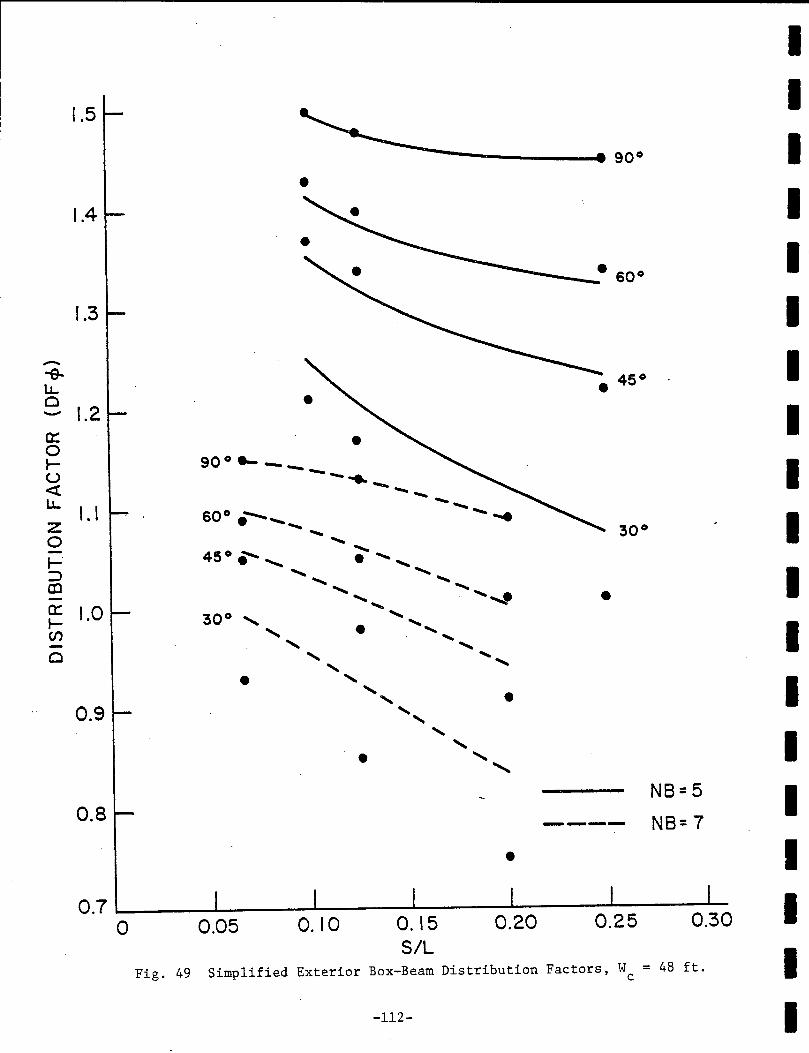
I
1.5 I
goo I •
1.4 I I
1.3 I - I -9-lJ..
45° • Q • - 1.2 I 0::: • 0 .,.._ gooe- __
I (.) -- ..... <t --lJ.. -1.1 ----z 60° .-.......__ --- .... I ..... 30° 0
..... ..... 45° ............
..... .,.._. . ..... :::> ........ .............
I IIl ..... .....
........ ..... 0:::
..... .....~ • 1.0
..... .,.._ 30° '
..... (/) ' • ,,
I - ' .... .....
Q ' ....
' .....
• ' I ' • 0.9 ' ..... .....
' ' I • ' ....... NB=5 I 0.8 ---- NB=7
• I 0.7 I 0 0.05 0.10 0.15 0.20 0.25 0.30
S/L I Fig. 49 Simplified Exterior Box-Beam Distribution Factors, w = 48 ft.
c
-112- I

I I
1.5
I I 1.4
I goo
I 1.3 goo e..... ---I -.... - ---&-
60°' • ............ LL... --0 . ....... • .... ...... 60°
I - 1.2 ...... 0:: 45°' ''--.
' ............. 0 ......
I 1- • ........ ............ u ...... ...... ...... <t ""' 45° LL.. 30°
' ~ • 1.1 ' • I z ,.
0
' 1- ' • I
::::> ' CD ' 0:: ' 1.0 • ' 1- ......
I (/')·
' 30° - ' 0 • ' ' ....
I • 0.9
I • NB=8 I 0.8 ---- NB=9
I 0.7
I 0 0.05 0.10 0.15 0.20 0.25 0.30 S/L
I Fig. so Simplified Exterior Box-Beam Distribution Factors, w = 72 ft. c
I -113-

9 . REFERENCES
1. American Association of State Highway Officials, STANDARD SPECIFICATIONS FOR HIGHWAY BRIDGES, lOth Edition, Washington, D. C., 1969.
2. American Association of State Highway Officials, STANDARD SPECIFICATIONS FOR HIGHWAY BRIDGES, 11th Edition, Washington, D. C., 1973.
3. American Association of State Highway and Transportation Officials,
STANDARD SPECIFICATIONS FOR HIGHWAY BRIDGES, Interim Specifications, Washington, D. C., 1974.
4. Bathe, K., Wilson, E., and Peterson, F. SAP IV, A STRUCTURAL ANALYSIS PROGRAM FOR STATIC AND DYNAMIC RESPONSE OF LINEAR SYSTEMS, Earthquake Engineering Research Center Report No. EERC 73-11, University of California, Berkeley, 1974.
5. Bogner, F. K., Fox, R. L. and Schmidt, L.A. THE GENERATION OF INTERELEMENT COMPATIBLE STIFFNESS AND MASS MATRICES BY THE USE OF INTERPOLATION FORMULAS, Proc. Conference on Matrix Methods in Structural Mechanics, Wright Patterson Air Force Base, Dayton, Ohio, October 1965.
6. Burdette, E. G. and Goodpasture, D. W. FINAL REPORT ON FULL SCALE BRIDGE TESTING: AN EVALUATION OF BRIDGE DESIGN CRITERIA, Department of Civil Engineering, University of Tennessee, December 1971.
7. Chen, Chiou-Horng and VanHorn, D. A. STATIC AND DYNAMIC FLEXURAL BEHAVIOR OF A PRESTRESSED CONCRETE I-BEAM BRIDGE - BARTONSVILLE BRIDGE, Fritz Engineering Laboratory Report No. 349.2, January 1971.
8. Chen, Chiou-Horng and VanHorn, D. A. STRUCTURAL BEHAVIOR OF A PRESTRESSED CONCRETE I-BEAM BRIDGE - LEHIGHTON BRIDGE, Fritz Engineering Laboratory Report No. 349.4, October 1971.
9. Chen, T. Y., Siess, C. P. and Newmark, N. M. MOMENTS IN SIMPLY-SUPPORTED SKEW I-BEAM BRIDGES, Studies of Slab and Beam Highway Bridges, Part IV, University of Illinois Engineering Experiment Station Bulletin No. 439, Urbana, Illinois, 1957.
-114-
I I I I I I I I I I I I I I I I I I I

I I I I I I I I I I I I I I I I I I I
10. Clough, R. W. and Tocher, J. L. FINITE ELEMENT STIFFNESS MATRICES FOR THE ANALYSIS OF PIATE BENDING, Proc. Conference on Matrix Hethods in Structural Hechanics, Wright Patterson Air Force Base, Dayton, Ohio, October 1965.
11. Dawe, D. J. PARALLELOGRAM ELEMEl.'tTS IN THE SOLUTION OF RHOI-.IBIC CANTILEVER PlATE PROBLEMS, Journal of Strain Analysis, Vol. l, No. 3, pp. 223-230, 1966.
12. DeCastro, E. s. and Kostem, C. N. LATEP.AL LOAD DISTRIBunm~ I.H ·sKEHED PRESTRESSED CONCRETE t-BEAJ1 BRIDGES, Fritz Engineering Laboratory Report no. 400.16:. July 1975.
13. DeCastro, E. S. and Kostem, C. N. USER'S K~NUAL FOR PROGRAH PLATE, Fritz Engineering Laboratory Report No. 400.13, January 1975.
14. DeCastro, E. S. and Kostem, C. N. USER'S MANUAL FOR PROGRAM INPT, Fritz Engineering Laboratory Report No. 400.18, July 1975.
15. DeCastro, E. S. and Kostem, C. N. USER'S MANUAL FOR PROGRAM SKBRD, Fritz Engineering Laboratory Report No. 400.15, June 19.75~.
16. Douglas, W. J. and VanHorn, D. A. LATERAL DISTRIBUTION OF STATIC LOADS IN A PRESTRESSED CONCRETE BOX-BEAM BRIDGE·- DREHERSVILLE BRIDGE, Fritz Engineering Laboratory Report No. 315.1, August 1966.
17. Felippa, C. A. REFINED FINITE ELEMENT ANALYSIS OF LINEAR AND NONLINEAR TWO-DI}ffiNSIONAL STRUCTURES, SESM Report 66-22, Department of Civil Engineering, University of California, Berkeley, October 1966.
18. Felippa, C. A. and Clough, R. w. A REFINED QUADRILATERAL ELEMENT FOR ANALYSIS OF PLATE BENDING, Second Conference on Matrix Methods in Structural Mechanics, Wright Patterson Air Force Base, Dayton, Ohio, October 1968.
19. Gaylord, H. and Gaylord, N., Editors STRUCTURAL ENGINEERING HANDBOOK, McGraw Hill, Ne-.;v York, 1968.
20. Green, A. E. and Zerna, W. THEORETICAL ELASTICITY, Clarendon Press, Oxford, 1954.
-115-

21. Guilford, A. A. and VanHorn, D. A. lATERAL DISTRIBUTION OF VEHICUlAR LOADS IN A PRESTRESSED CONCRETE BOX-B~ BRIDGE - WHITE HAVEN BRIDGE, Fritz Engineering Laboratory Report No. 315.7, August 1968.
22. Guilford, A. A. and Va~qorn, D. A. lATERAL DISTRIBUTION OF VEHICUlAR LOADS IN A PRESTRESSED CONCRETE BOX-B~ BRIDGE - BERWICK BRIDGE, Fritz Engineering Laboratory Report No. 315.4, October 1967.
23. Gustafson, W. C. and Wright, R. N. ANALYSIS OF SKEWED COMPOSITE GIRDER BRIDGES, Journal of the Structural Division, Proceedings of the ASCE, Vol. 94, ST4, pp. 919-941, April 1968.
24. High\vay Research Board THE AASHO ROAD TEST, Report 4, Bridge Research, Special Report 610, National Academy of Sciences, 1962.
25. Hondros, G. and ~~rsh, J. G.· LOAD DISTRIBUTION IN COMPOSITE GIRDER SlAB BRIDGES, Journal of the Structural Division, Proceedings of the ASCE, Vol. 86, ST11, pp. 79-109, November 1960.
26. Jensen, V. P. ANALYSIS OF SKEW SlABS, University of Illinois Engineering Experiment Station Bulletin, No. 332, Urbana, Illinois, 1941.
27. Jumppanem,. P •. BENDING OF PARALLELOGRAM PlATES, Acta Polytechnica Scandinavica, Civil Engineering and Building Construction Series No. 61, Helsinki, 1970.
28. Kennedy, J. B. and Simon, J. G. LINEAR AND NONLINEAR ANALYSES OF SKEWED PlATES, Journal of Applied Mechanics, Vol. 34, p. 2, 1967.
29. Kostem, C. N. ANALYTICAL MODELL~G OF BEAM SlAB BRIDGES, Proce~dings of the International Symposium on Folded Plates and Spatial Panel Structures, Udine, Italy, September 1974.
30. Lehigh University Computing Center THE LEAPS USER'S GUIDE A!~ MANUAL, Lehigh University Computing Center, Bethlehem, Pennsylvania, May 1973.
31. Lin, Chen-Shung and VanHorn, D. A. THE EFFECT OF MIDSPAN DIAPHRAGMS ON LOAD DISTRIBUTION IN A PRESTRESSED CONCRETE BOX- BEAM BRIDGE - PHilADELPHIA BRIDGE, Fritz Engineering Laboratory Report No. 315.6, June 1968.
-116-
I I I I I I I I I I I I I I I I I I I
I I I I I I I I I I I I I I I I I I I
32. Macias-Rendon, M. A. and VanHorn, D. A. ~10DEL STUDY OF BEAM SlAB BRIDGE SUPERSTRUCTURES, Journal of the Structural Division, Proceedings of the ASCE, ST9, Vol. 99, pp. 1805-1821, September 1973.
33. Meek, J. L. MATRIX STRUCTURAL ANALYSIS, McGraw Hill, New York, 1971.
.34. Melosh, R. J. BASIS FOR THE DERIVATION OF MA.TRICES FOR THE DIRECT STIFFNESS METHOD, AIAA Journal, Vol. 1, No. 7, July 1963.
35. Monforton, G •. R •. and Schmidt, L.A. FINITE ELEMENT ANALYSIS OF SKEW PlATES IN BENDING, AIAA Journal, Vol. 6, No. 6, pp. 1150-1152, 1968.
36. Morice, P. B. and Little, G. ANALYSIS OF RIGHT BRIDGES SUBJECTED TO NOID-IAL LOADING, Cement and Concrete Association, London, D.B.ll.
37. Morley, L. S. D. SKEW PlATES AND STRUCTURES, Pergamon Press, McMillan Company, New York, 1963.
38. Motarjemi, D. and VanHorn, D. A. THEORETICAL ANALYSIS OF LOAD DISTRIBUTION IN PRESTRESSED CONCRETE BOX-Bruu~ BRIDGES, Fritz Engineering Laboratory Report No. 315.9, October 1969.
39. Newmark, N. M. and Siess, C. P. ~MENTS IN I-BEAM BRIDGES, University of Illinois Engineering Experiment Station Bulletin No. 336, Urbana, Illinois, 1942.
40. Newmark, N. M., Siess, C. P. and Pechham, W. M. TEST OF SIMPLE SPAN RIGHT I-Bruu~ BRIDGES, Studies of Slab and Beam Highway Bridges: Part I, University of Illinois Engineering Experiment Station Bulletin No. 363, Vol. 43, No. 42, Urbana, Illinois, March 1946. ·
41. Newmark, N. M., Siess, C. P. and Pechham, W. M. TEST OF SIMPLE SPAN SKEW I-BEAM BRIDGES, Studies of Slab and Beam Highway Bridges, Part II, University of Illinois Engineering Experiment Station Bulletin No. 375, Vol. 45, No. 31, Urbana, Illinois, January 1948.
42. Pennsylvania Department of Highways S~NDARDS FOR PRESTRESSED CONCRETE BRIDGES, ST200-ST208, Bureau of Design, Bridge Division, Commonwealth of Pennsylvania, 1960.
-117-

43.
44.
45.
46.
47.
48.
49.
50.
51.
Pennsylvania Department of Transportation STANDARDS FOR BRIDGE DESIGN, BD-201~ Bureau of Design, Commonwealth of Pennsylvania, June 1973.
Pickett~ G. APPLICATION OF THE FOURIER METHOD TO THE SOLUTION OF CERtaiN BOUNDARY PROBLEMS IN THE THEORY OF ELASTICITY, Journal of Applied Mechanics, Vol. 11~ p. 176, 1944.
Przemieniecki, J. S. THEORY OF }fATRIX STRUCTURAL ANALYSIS~ McGraw Hill, New York, 1968.
Rai, S. I. and Sandhu, S. R. FINITE ELEMENT OF AN ISOTROPIC PlATE USING Q-19 ELEMENT, PART I, THEORETICAL DEVELOPMENT, Ohio Univer'sity and Air Force Flight Dynamics Laboratory, AFFDL-TR-74-120, Wright Patterson Air ~orce Base, Ohio, October 1974.
Robinson, K. E. THE EFFECT OF SKEW ON THE BEHAVIOR OF SIMPLY SUPPORTED BRIDGE SLABS, Cement and.Concrete Association, Technical Report TRB/271, July 1957.
II
Rusch, E. H. and Hergenroder, A. EINFLUBFELDER DER MOMENTE SCHREF-WINKLIGER PlATTEN (Influence Surfaces for Moments in Skew Slabs) Werner-Verlag, Dusseldorf, 3rd Ed., 1969, Translated by C. V. Amerongen.
Sanders, W. W., Jr. and Elleby, H. A. DISTRIBUTION OF WHEEL LOADS IN HIG~ BRIDGES, National Cooperative Highway ResearCh Program, Report No. 83, Highway Research Board~ Washington, D. C., 1970.
Sandhu, S. R. . FINITE ELEMENT ANALYSIS OF AN ISOTROPI.'C PlATE USING Q-19 ELEMENT, PART II, INSTEUCTION FOB.. USERS AND FORTRAN LISTING, Ohio State University and Air Force Flight Dynamics Laboratory, Wright Patterson Air Force Base, Ohio, October 1974.
Schaffer, T. and VanHorn, D. A. STRUCTURAL RESPONSE OF A 45° SKEW PRESTRESSED CONCRETE BOX-GIRDER BRIDGE SUBJECTED TO VEHICUlAR LOADING -BROOKVILLE BRIDGE, Fritz Engineering Laboratory Report No. 315.5, October 1967.
-118-
I I I I I I I I I I I I I I I I I I I

I I I I I I I I I I I I I I I I I I I
52. Schultchen, E. G. and Kostem, C. N. USER'S MANUAL FOR CSTPL FINITE ELEMENT PROGRAM, Fritz Engineering Laboratory Report No. 400.2, June 1971.
53. Sisodiya, R. G. and Cheung, Y. K. A HIGHER ORDER IN-PlANE PARALLELOGRAM EID1ENT AND ITS APPLICATION TO SKEWED CURVED BOX-GIRDER BRIDGES, Developments in Bridge Design and Constructions, Rockey et al, Editors, Crosby, Lockwood and Sons Ltd., London, 1971.
54. Timoshenko, S. P. and Goodier, V. N. THEORY OF ElASTICITY, 3rd Edition, McGra\v Hill, New York, 1970.
55. Timoshenko, S. P. and Woinoswki-Krieger, S. THEORY OF PlATES AND SHELLS, 2nd Edition, NcGra\v Hill, New York, 1959.
56. Tottenham, H. and Brebbia, C. (Editors) FINITE ELEMENT TECHNIQUES IN STRUCTURAL MECHA.NICS, Stress Analysis Publishers, Southampton, England, 1970.
57. VanHorn, D. A. STRUCTURAL BEHAVIOR CHARACTERISTICS OF PRESTRESSED CONCRETE BOX-BEAM BRIDGES, Fritz Engineering Laboratory Report No. 315.8, December 1969.
58. Wegmuller, A. W. and Kostem, C. N. FINITE ELEMENT ANALYSIS OF PlATES AND ECCENTRICALLY STIFFENED PLATES, Fritz Engineering Laboratory Report No. 378A.3, February 1973.
59. William, K. J. FINITE ELEMENT ANALYSIS OF CELLUlAR STRUCTURES> Ph.D. Dissertation, University of California, Berkeley, 1969 •
. 60 •. William, K. J. and Scordelis, S. C. COMPUTER PROGRAM FOR CELLUlAR STRUCTURES OF ARB! TRARY PLAN GEOMETRY, SESM Report 70-10, Department of Civil Engineering, University of California, Berkeley, 1969.
61. Yen, B. T., Chen, Y. S., et al MODEL TESTS ON CO~~OSITE BOX-BEAMS, Fritz Engineering Laboratory Report No. 380.6, October 1973.
62. Zellin, M. A., Kostem, C. N. and VanHorn, D. A. LOAD DISTRIBUTION OF LIVE LOAD IN PRESTRESSED CONCRETE I-BEAlfBRIDGES, Fritz Engineering Laboratory Report No. 387.2A, June 1975.
-119-

63. Zellin, M.A., Kostem, C. N. and VanHorn, D. A. STRUCTURAL BEHAVIOR OF BEAM-SLAB HIGHWAY BRIDGES, A Summary of Completed Research and Bibliography, Fritz Engineering Laboratory Report No. 387.1, May 1973.
64. Zienkiewicz, 0. C. and Cheung, Y. K. THE FINITE ELEMENT METHOD IN STRUCTURAL AND CONTINUUM MECHANICS, McGraw Hill, New York, 1967.
65. Zienkiewicz, 0. C. and Hollister, G. S. STRESS ANALYSIS, John Wiley and Sons, New York, 1975.
66. deCastro, E. S. and Kostem, C. N. LOAD DISTRIBUTION IN SKEWED BEAM-SLAB HIGHWAY BRIDGES, Fritz Engineering Laboratory Report No. 378A.7, December 1975.
-120-
I I I I I I I I I I I I I I I I I I I

I I I I I I I I I I I I I I I I I I I
10. APPENDICES
Appendix A FINITE ELEMENT ANALYSIS OF SKEWED ELASTIC
PLATES
A1. Q8S11 ELEMENT STIFFNESS MATRIX
A2. COMPATIBLE DISPLACEMENT FUNCTIONS FOR
PLATE BENDING ELEMENT Q-19
Appendix B FINITE ELEMENT ANALYSIS OF SKEWED STIFFENED
PLATES
-121-

APPENDIX A
FINITE ELEMENT AN~YSIS OF SKEWED ELASTIC PLATES
A.l Ske~y Plate In-Plane Analysis
The skew~late also known as a parallelogram is a special
case of a quadrilateral plate 't¥hen opposite sides are para_llel
(Fig. Al). The acute angle between two adjacent sides is called the
skew angle as shown in the figure. The rectangular plate is a special
case of·. the skew plate when the skew angle is 90°.
A.l.l Methods of Solutions
The solutions to skew in-plane problems have been arrived at
by using the theory of elasticity in rectangular~oblique and polar co-
ordinate systems (Ref. 37). As reported by Horley in Ref. 37, solu-
tions in rectangular and oblique coordinates have been obtained by
Hemp, Favre, Lardy and Theodorescu; and solutions in the polar coordi-
nate system have been obtained by Coker and Filon, Williams, and
Mansfield. Solutions in terms of the Airy stress function expressed
in complex variables, trigonometric series, and infinite series have
been obtained by Green and Zerna (Ref. 20) and Pickett (Ref. 44).
A.l. 2 Assumptions and Basic Equations
The skew plate under any in-plane forces is assumed to be a
plane stress problem. Stresses a , a and 1" and the generalized X y xy ..
forces N , N and N in an infinitesimal element are shcnm in Fig. A2. X y xy
The components of stress and generalized forces shown in the figure
indicate the assumed positive direction. The generalized forces are
the stresses integrated over the thickness of the element.
-122-
I I I I 1-I I I I I I I I I I I I I I

I I I I I I I I I I I I I I I I I I I
'·
The .displacement at any 'point of the plate is defined by the
components of the vector field {v}:
{v}= {:} ~.1)
where- u and v are in the x and y directions respectively. Th~ ·strain
field at ~ny point is defined from the displacement field by the
relationship:
e: au XX ax
{e:} = av e: = yy ay
Yxy au+ av ay ax
where e:xx, e:yy' Yxy are the well known components of strain.
The usual stress-strain relationship ({cr} T [D] {e:})
for the general orthotropic case is given by Ref. 64:
cr X
a y
T
E =
. xy
where E - ,_-- n = _.1.. _ ... :: E.
2
G m=~
E 2
.:: ... '.:.
n n\,1 2 0
0\,1 2
1 0
0 0 m(l - n"' 2) 2
-123-
e: X
(A. 2)
(A.3)

I .
..
in which E and E are the principal elastic moduli in the x and y 1 2
direction, v is the Poisson's ratio, and G is the shear modulus. . 2 2
For the isotropic case, E 1
= E ' 'J 2 2
1 = v, and m = 2 (1 + v)'
A.2 In-Plane Finite Element Analysis of Skew Plates
A.2.1 Geometry and Displacement Field
Consider a quadrilate~al in-lane finite element as shown in
Fig. A3.. The local coordinate system with the origin at the centroid of
the element is indicated by ' and 11· The nodes are numbered counter-
clockwise with the node at the centroid being the fifth node. The
edges 1-2 and 3-4 of the quadrilateral are represented by ' = -1 and
z; = 1. The edges 2-3 and 4-1 are represented by 11 = -1 and 11 = 1.
The in-plane element has eight external and three internal
degrees of freedom (Fig. A3). The external degrees of freedom are the
displacements ui and vi specified at the external nodes i, 1 = 1 to 4.
The three internal degrees of freedom are the displacements u and v s 5
and the strain y • xy
fifth node while the
The displacement u . and v are specified at the 5 s
strain y is assumed to be constant throughout xy
the element. This element was originated by Doherty who designed the
element based on physical concepts and was derived by Williams using l;
concise variational formulation "(Ref. 59) •
The geometrical relationships between the global3coord~ates and the local coordinates can be expressed in matrix form by the fol-
lowing expressions: .
-124-
I I I I I I I I I I I I I I I I I I I

I I I I I I I I I I I I I I I I I I I
CJ (A.4)
where ~ = 1 (1 + ~~ ) (1 + nni) X 4 i
in which xi and yi are the global coordinates of node i, and ni and ~i
are the local coordinates of node i.
The displacement function for the element is assumed to be a
linear shape function for the corner points and a quadratic interpola-
tion function for the interior point. The internal shape function
selected is the quadratic interpolation scheme with vanishing values at
the boundaries (Ref. 59). Thus, the equation {v} = [<P] {v.}, .for this 1.
element, can be written as follows
where, ., '
0 f 0 f 2 3
£ 0 f 0 1 2
v 1
u v v 2 2 !
0
f !
f It
0
v u s It
-125-
0
£ It
f 5
0
v u It 5
:.] (A. 5)
(A.5a)

and, f 1 (1 - n) = - (1 - I;) (A. Sb)
1 4
f =.!. (1 + I;) 2 4
(1 - n) (A.Sc)
1 (1 + n) f = - (1 + I;) (A.Sd) 3 4
f 1 (1+ n) (A. Se) =- (1 - I;) .. . 4
f = (1 - 1',;2) (1 - n2) (A. Sf) 5
A.2.2 Derivation of Element Stiffness Matrix
'The strain field can be derived from the standard strain dis-
placement relationship. With the assumption of constant shear strain
and with the additional strain degree of freedom, the strain components
can be written (Ref. 59)
e: u 0 0 XX:
e: = 0 v 0 (A.6) YY
yxy 0 0 1 a
where 3fi u =ax (A.6a)
3fi V=-
3y
·., :·
(A6-:-b)
and a is the generalized coordinate associated with the constant shear
strain degree of freedom. The derivatives of the functions in
Eqs. A.6a and A.6hcan be written with the help of the chain rule
(Ref. 45):
-126-
I I I I I I I I I I I I I I I I I I I

I I I I I I I I I I I I I
I I I I I
' a£ h 3£
k a£i
i i .~· an - an • az;
-= (A. 7) ax ax Ez ax Ez az; an an ar;
a f. ax afi ax afi
l. an • an - an • az; ay = ax h ax h (A. 8)
-az; an an az;
The evaluation of the element stiffness for the resulting
finite element model is given in Appendix Al. The final stiffness
matrix is obtained by the application of the static condensation proce-
dure on the interior node as described in Refs. ·17 an-1 18. The element
is known as Q8Dll.
The explicit integration of the stiffness matrix integral is
a lengthy process and difficult. The usual procedure in this case is
to use the numerical integration procedure (Refs. 45,59,64).
In the procedure, the terms of the matrices are evaluated at
several points call integration points. The Gaussian quadrature formu-
lation is found to be most useful for the present problem. In the
formulation, the polynomial function is integrated as the s~ of the
weighted values at specified points.
1 Thus, a function /_
1 f(<;)d<; can be replaced by a summation
.. ~ :: .. : . n J
1 f(<;)d<; = E wj f(a.)
-1 . j=1 J (A. 9)
-127-

where W. are the weight coefficients and a. are the values of the J J
function at the n specified points.
The double integral of the form
1 l
·I = J J £ (,,~) d' dn (A.lO) -1 -1
can be replaced by the following summation (Ref. 64):
n n I = ~ ~ W. W. f (a., b
1)
i=l j=l J l. J (A.ll)
The numerical values of the coordinates at the integration
points and the weight coefficients for ~ifferent values_of n are
given by Zienkiewicz (Ref. 64). For this element, William has shown
that the 2 x 2 Gaussian quadrature formula provides better results
in stiffness than the improved 3 x 3 Gaussian integration scheme
(Ref. 59). The coordinates of the integration points are shown in
Fig. A4 and the weight coefficients are equal to 1 (Ref. 64).
The following should be noted in connection with this
element. First, since a different shape function is used to describe
individual displacement and strain components, the variation of
displacement is not homogeneous. The stiffness property of'the
element is therefore directional. Secondly, monotonic convergence
and boundedness is lost according to the Melosh crlt~riori (R~f. 34).
This c;iterion requires that interpolation function ot' .int"ern.k-1 nodes ::·•.'·
must be lower than the external.node. However, this element has
been shown to give more flexible and better results among the 8
degree of freedom family. ~isplacement models (Ref. 59).
-128-
I I I I I-I I I I I I I I I I I I I I

I I I I I I· I I I I I I I I I I I I I
The Q8Dll element has been testea and compared with other
finite elements by William (Ref. 59). The same study showed_ the
efficiency and accuracy of the element among the other finite
elements. This element will be combined with the plate bending
element in Section A.4 to make up the basic plate element used in
this study. Numerical examples are provided to illustrate the
accuracy of the element.
A.2.3 Numerical Examples and Comparisons
The accuracy of the finite element solution for rectangular
plate problems as compared with theoretically exact answers has been
reported and shown by Zienkiewicz, and Tottenham and Brebbia (Refs.
56,64). Unfortunately, very little data is available for skew plate
problems except for the very simple cases.
The method of analysis must be applicable for all angles of
skew. Therefore, the first test example is a rectangular plate under
uniform edge loading and under pure shear loading. The plate proper-
ties and dimensions are shown in Fig. A.S. The skew angle is 90° and
the exact solution can be found from the theory of elasticity. The
results. are tabulated in Tables Al and A2. · It can be noted that uni-~ ; ·.: -· :·
form strain for these loadings is accurately predicted by the element • . ·. ·..: '
The CST, that is, constant strain triangle (Ref. 52), finite element ' . :: ~ > -
-129-
. '
solution ~s also shown in Tables Al and A2 for comparison. The CST dis
cretization in this example was with the use of 8 triangular elements
formed by connecting two opposite corner nodes of the complete plate
and connecting the midpoints of opposite sides.
The second example is a skew plate under uniform edge loading
as shown in Fig. A6. The state of stress for this problem is uniform
throughout the element and can be found directly from equilibrium. The
example illustrates the applicability of the element to plate problems
with a parallelogram shape. The discretization into four rhombic ele
ments is shown in Fig. A6b. The discretization into eight triangular
elements for the CST analysis follows the same procedure as the first
example. The numerical results are tabulated in Table A3. Since the
exact solution is that of constant strain, the analytical results veri
fied the analytical model.
The third example is a skew plate under in-plane concentrated
loads. The plate shown in Fig.A7 is fixed at the supports and sub-
jected to two concentrated loads near midspan. This problem is chosen
to illustrate the accuracy of the element under this type of loading.
There is no exact solution for this problem. The solutions are pro
vided by using linear strain equilateral -LSE (Ref •. 60), constant
strain triangle -CST (Ref. 52), and the reported values from. Ref. 59.
The results are tabulated in Table A4.
r• .,! -. .
·.: ' Q8D8 refers to the quadrilateral element with only four nodes
and twc~(degrees of freedom at each node. Q8Dll(3) refers to the de
rived finite element using the 3 x 3 integration rule. The Q8Dl1(2)
-130-
I I I I I I I I I I I I I I I I I I I

I '
I I I I I I I I I I I I I I I I I '
' "·
refers to the element formulation using the 2 x 2 integration rule.
The accuracy of the element using the relaxed integration rule
can be seen from the table.
The final example is the problem of the beam with inclined
faces under a concentrated load at midspan. The structure is showntn
Fig. A8a and the two selected discretizations are shown in Figs~ A8b
and A8c. The analytical solution is compared to the solution by
Sisodiya and Cheung (Ref. 53) who used a higher order element that
gives good results for the given type of structure and loading. The
results are tabulated in Table AS. The advantage of the element over
the standard Q8D8 is made obvious in this example.
It should be emphasized that this example is the most severe
case the element will be subjected to. In the application of this
element to the beam slab problem, the element will represent the
in-plane behavior of the deck slab. As such, the typical type of load-
ing would be in-plane loads in the direction of span thus producing
column behavior rather than beam behavior. The results of this example
are the reasons for the choice of another element to represent the
in-plane behavior of webs for box-beam bridges in Chapter 4.
... . :-~
A.3 Skew Plate Bending Analysis
A. 3.1 Methods of Solutions
The- exact solution to the differential equation of skew
plates in bending is difficult to obtain if at all possible. F?f the
-131-

simple cases, the problem is solved by direct integration of the dif
ferential equation under associated boundary conditions~ or by the
application of conformal mapping (Ref. 27). Subsequently, a number of
studies have been concerned with investigations of the methods of solu
tion, the most common being the series solutions and the method of
finite difference (Ref. 26). Solutions iri oblique coordinates, trigo
nometric series, and finite difference solutions by several authors are
listed and referenced by Morley in Ref. 37. Solutions by polynomials
and trigonometric functions have been obtained by Jumppanem (Ref. 27)
and Kennedy and Simon (Ref. 28) •
Based on model tests Rusch (Ref. 48} produced design data in
the form of influence surfaces for bending and torsional moments of
simply-supported slabs with various angles of skew. A series of thir
teen skew slab models of different side to length ratio were investi
gated. The slab models tested were all simple span structures and made
of gypsum plaster. As in any model study, it was not possible to inves
tigate all parameters.
One of the earliest solutions using the finite difference
methods was made by Jensen (Ref. 26). This was followed by Chen et al.
in 1957 and by Robinson in 1959 (Refs. 9, 47).
Within the past decade, the finite element technique has been
employed successfully to analyze plates of arbitrary shape (Refs. 5,10,
18). Zienkiewicz and Cheung, and Melosh used the technique to analyze
plates in bending (Refs. 34,64) using rectangular elements. Based on
the same deformation pattern used in the rectangular plate element
-132-
I I I I I-I I I I I I I I I I I I I I

I I I I I I.
I I I I I I I I I I I I I
Dawe (Ref. 11) developed the stiffness matrices for parallelogram ele
ments. Subsequently triangular elements were introduced, the most com
mon being those by Zienkiewicz and Cheung (Ref. 64) and by Clough and
Tocher (Ref. 10). Further improvements in accuracy were subsequently
obtained by Felippa and Clough (Ref. 18) , and Bogner et al. ·(Ref. 5)
with the ·use of refined and higher order elements.
A.j.2 Assumptions and Basic Equations
A typical element from a skew plate structure is shown in
Fig. A9. The element is of differential dimensions whose sides are
parallel to the orthogonal x-y system of coordinates. The reference
plane is assumed ~o lie on t.he mid-plane of the plate. Forces, dis
placements and the adopted sign conventions are shown in the positive
directions in Fig. A9. The plate is assumed to be elastic, homogeneous,
orthotropic and of uniform thickness, t. The standard assumptions in
small deflection theory of plates are employed:
1. Stresses normal to the plate are negligible
2. Deflections are small relative to the plate thickness
3. Deflection in the z direction is a function of x and y only
4. Shear strains yxz, yYz in the x andy fac~s ·of the element
and·iri the direction of z are equal to zero.
The consequence of the above assumptions is that normals to
the plate remain normal after deformation.
-133-

From the above assumptions, the displacement· equations may be
written as: U(z) = u - z ~ (A.12a)
V(z) = v- z ~ (A.l2b)
where U(z) and V(z) are the displacement components of the point at
distance z from the reference plane; and u, v, and w are the displace-
meut components of the point on the reference plane.
Equations A.12a and A. 2b can be differentiated to obtain the
relationship of the strains to displacements:
au a2w € ax - z-·
X 3:x2
av 32w (A.13) € = ay - z-y az2
au + av - a2w Yxy
2z-ay ax axay
The ~tress-strain relationship given by Eq. A.3 in Section A.1.2 can
'then be rewritten explicitly by substituting the above expressions for
€ ' E and y :
X y :xy
c ( au a2w ) +C ( av a'w J a = ax - z -- -- z--
X 11 ax2 12 ay ay2 (A.14a)
( au . 32w ) +C ( av a2w )
a = c ax - z- 3y - z--y 21 ax~
22 3y2 (A.14b)
-134-
I I I I I I I I I I I I I I I I I I I
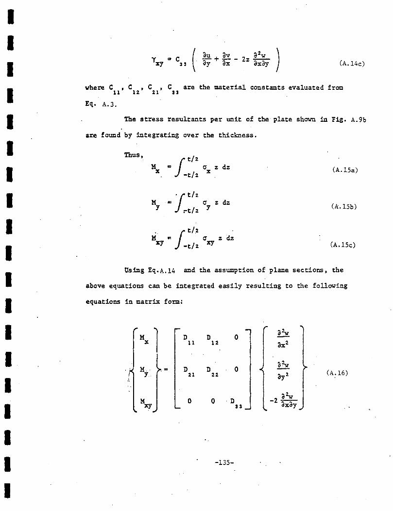
I I I I I I I I I I I I I I I I I I I
v = c· ( dU + dV _ Zz 32w )
1rj 33 . Cly dX dXdY (A.l4c)
where C , C , C , C are the material constants evaluated free 11 12 21 33
Eq. A.3.
The stress resultants per unit of the plate shown in Fig. A.9b
are found by integrating over the thickness.
Thus,
M f t/2
a z dz X "" -t/2 X (A.l5a)
M f t/2 z dz Y .. ~t/2. cry (A.l5b)
.. I t/.2 M a: a zdz rj -t/2 xy (A.l5c)
Using Eq.A.l4 and the assumption of plane sections, the
above equations can be iotegrated easily resulting to the following
equations in matrix fo~:
M l D D 0 a2v
X 11 12 dX2
M. D D 0 a~ = (A.l6) ; Y. 21 22 3y2
i:'
M 0 0 ·D 2 a>w J xy 33 - 3x3y
-135-

where c t3 D = 11
11 12
c t3 D = D = l2
12 21 12
c t' D Cl 33
53 12
Equation· A.l6 is the explicit form of the equation {cr} = [D]{£}
applied to plate bending.
A.4 A Finite Element Analysis of Skew Plates in Bending
In this section, the general quadrilateral element is pre-
sented. The elament is developed by Felippa and reported in Ref. 18.
This element is employed in the reported investigation. The element
has been tested \mder a variety of boundary conditions and the results
compare favorably with the theory of elasticity solutions (Ref. 18).
The quadrilateral element is a confoDming element formed from
four triangular elements whiCh satisfy deflection and slope continuity
along the boundaries. Each one of the triangular elements is known as
the LCCT-11 or the linear curvature compatible triangle with eleven
fundamental degrees of freedom. The LCCT-11 is a simplified form of ;.:::: ..
the triangular element LCCT~12 which has twelve degrees of freedom. . . ~
The LCCT-11 is obtained from LCCT-12 by imposing the linear variation
of the slope normal to one side of the triangle.
-136-
I I I I a-
I I I I I I I I I I I I I I
I I I I I I I I I I I I I
I I I I I
·The elem~nt formulation is outlined in the following sec-
tions. Detailed derivations can be found in Refs. 17, 46 and SO.
A.4.1 Element Coordinate Systems
'Ihe geometry of a triangular element can be expressed by the
projected dimensions in cartesian coordinate system (Fig •. AlO), by
intrinsic dimensions (Fig. All), or by dimensions in the natural coordi-
nate system (Fig. Al2).
In Fig. A12,A , A , A are the three subtriangles subtended 1 2 1
by point P such that
(A.17)
where the index i = 1, 2, or 3 designates the number of the corner
opposite to Ai and A is the total area of the complete triangle.
From Fig. All, Eq. A.l7 can also be written as
(A.l8)
where n. is the normal distance of point P and h. is the height of ~ ~
node i from side i. These relationships are used to simplify the
expressions in ·the element stiffness formulations.
The relationship between cartesian and natural coordinates
is expressed as follows (Ref. 33):
-137-;_

1 1 1 1 1;;1
X = X X X ?;; 1 2 s 2 (A.l9)
·• ·. . ~..y y1 y2 y! ?;; !
where x1
·and y1
are the coordinates of the nodes i, i=l, 2, 3.
The inverse relationship can be obtained by solving·for 1;;1,
z;2, and?; from Eq. A.l9: 3
1;;1 2A b a 1 1 1 1
1;;2 1 2A b =- a X (A. 20) 2A 2 2 2
?;;· 2A b" a y 3 s 3 3
where ai and bi are the proje~ted dimensions shown in Fig. AJO.
The derivatives of a function f(1; , 1; , ?;; ) with respect to 1 2 s
the x, andy axes and a normal n. can be obtained by the chain rule I l.
(Ref. 33):
3f 1 ( 3£ b + 2L b + 3£. b ) ax =-2A 3?;; 1 ()?;; 2 3?;; 3
1 2 '
(A. 22)
(A. 23) 3£ 1 ( 3£ 3f 3£ )
3y = 2A 31;;1 a1 +~a2 + 3?;;s a3 1
-138-
I I I I 1-
I I I I I I I I I I I I I I

I I I I
I I I·
II I I I I I I I I I I I I
where coordinates di and ti are shown in Fig. All.
The above relationships are used in the formula~ion of the
element displacement field and stiffness properties in Se:ctions A.4.2 f.
and A.4. 3.
A.4.2 Construction of the Element Displacement Field
The twelve fundamental degrees of freedom for the LCCT-12
element at the external nodes of the triangular element are shown in
Fig.Al3. These can be expressed as components of the nodal displaca
ment vector. {r}:
. { r} T = . { w 8 8 w 8 8 . w3
8 .. 8 3
6, 8 5
8 6
} .1 Xl y1 · 2 x2 y2 x~ y ~
(A.24)
where wi, exi and eyi are the transverse displacement, rotation about
the x-axis~ and rotation about the y-axis respectively of node i. e , ~
e and e are normal slopes at the midside nodes of the element s 6
botmdar.ies.
As proposed by Felippa (Ref. 17) the element is subdivided
into three sub triangles or subelements as shown in Fig. Al3. Each sub-
element has three displacement components at each node and one rotation
component at the. midpoint of the outer side (Fig. Al3). Point 0 is
located at the centroid of the complete triangular element. Indepen-
dent cubic displacement functions.are then assumed for each subelement.
The nodal displacements for each triangle can be listed as
foll~s:
-139-

T {r(1)} = {w e e w e e w e e e }
2 X2 Y2 3 X3 Y3 0 xo yo s (A. 25a) ·
{r(2)}T = {w 9 e w e e w e e e l 3 X3 y3 1 X1 Y1 0 xo yo 6 (A. 25b)
{r(3)}T = {w 8 e w e e w e e e } 1 Xl Yl 2 X2 Y2 0 xo yo 7 (A. 25c)
Since each subelement has ten degrees of freedom a complete
cubic polynomial expression can be used (Ref. 18). Thus for sub element i:
(A. 26)
where [~(i)] is the interpolating polynomial that relates displacements
within the element to the nodal displacements by {v} = [~] {v.} .. . 1.
The explicit expression for ~(i) for i=l has been derived and presented
by Felippa in Ref~ 18:
r,; 2 (3 - 2r,; ) + 6ll (1
) r,; r,; r,; 1 1 3 1 2 3
r,;2 (b ( 1) r,; - b ( 1) r,; ) + (b ( 1) ll ( 1) ~ b ( 1)) ' ~ l,; 1; 1 3 2 2 3 3 3 1 123
~2 (a(1)~ - a(1)~ ) + (a(1)ll(l) - a (1)) ~ 1; l,;
1 3 2 2 3 3 3 1 1 2 3
7,;2 (3- 21;) + 6A(1
) ~ ~ r,; 2 2 3 1 2 3
T (b (1) r,; - b(1)l,;) + (b(l) - b( 1)A (1)) ~ (1) = r,;2 ~ l,; l,; (A. 27) 2 .3 3 1 2. 3 3 1 2 3
r,; 2 (3 - 2r,; ) 3 3
r,;2 (b(l)~ - b(l)~) 3 2 1 1 2.
-140-
I I I I I-I I I I I I I I I I I I I I
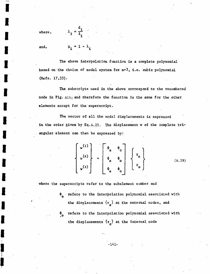
I I I I I I.
I I I I I I.
I I I I I I i i
'
where,
and,
di A =. i R. .
i
lli = 1 - A . i
The above interpolation function is a complete polynomial
based on ·the choice of nodal system for n=3, i.e. cubic polynomial
(Refs. 17,33).
The subscripts used in the above correspond to the renumbered
node in Fig. A14; and therefore the function is the same for the other
elements except for the·superscript.
The vector of all the nqda1 displacements is expressed
in the order given by Eq.A.25. The displacement w of the complete tri-
angular element can then be expressed by:
w (1)
~ ~ ·e 0
(2) r ~ ~
e w = (A. 28) e 0
w(3.) r
~ ~ 0
e 0
where the superscripts refer to th~ subelement number and
~ refers to the interPolation polynomial associated with e
the displacements {re} at the external nodes,. and
~ refers to the interpolation polynomial associated with .o
the displacements. {r } at the internal node 0
-141-

Transverse displacement of two adjacent subeiements are iden-
tical along the juncture line. However, along this line their normal
slopes differ. To impose slope compatibility along the internal edges,
additional nodes 7, 8 and 9 are located at midpoint of these edges
(Fig. Al5). The normal slopes are computed from Eq. A..21 and evaluated
at nodes 7, 8 and 9. The resulting compatibility equations are then
used to evaluate the displacements at the internal node. {r } in terms 0
of the displacements at the external nodes. {r }. e
The final displacement field is then written only in terms of
the external degrees of freedom:
w (1)
w (2)
= (A. 29)
w (3)
"'(i) The explicit expression for ~ is given in Appendix A2 for
ready reference.
A.4.3 Derivation of the Element Stiffness Matrix
The stiffness matrix for each subelement can be derived fol-
lowing th~ procedure outlined in Ref. 65 Uogether with the dis-
placement function given in Eq. A.2&~
From Eq. A.l6 {€} is defined to be:
-142-
I I I I I-I I I I I I I I I I I I I I

I I I I I I I I I I I I I I I I.
I I I
.. {E:} = (A.30)
and is known as the curvature field.
For subelement i, the curvature field can be obtained by pro-
per differentiation of the displacement function given by Eq. A. 28, and
the use of Eqs. A.22 and A.23
a2$(i) - 2 ~ax=-=a-y-
(A. 31)
The nodal values of the curvature can be obtained by evalu-
ating Eq. A.30 .at the nodes. Thus
.(A.32) ·
where {€(i)} is the vector of nodal curvatures and [~(i)] is the matrix c B
[T(i)] evaluated at the node points of element i.
-143-

The linear curvature variation within the subelement can now
be expressed in terms of the nodal curvatures by a linear interpolating
function [~E] such that
. {E (i)} = [~ (i)] {E (i)} (A. 33) E c
where z;l z; z; 0 0 0 0 0 o.
2. 3
[~ (i)] = 0 o. 0 z; z; z; 0 0 0 E 1 2. 3
0 0 0 0 0 0 z; z; z; 1 1 3
With Eqs. A.l6 and A.32, the stiffness matrix can
be evaluated:
(A. 34)
Since the stiffness matrix of a subelement is expressed in
terms of the same set of nodal coordinates, the stiffness matrix of the
complete triangular element is obtained by adding the contributions of
the three subelements, thus,
(A. 35)
Four of these triangular elements are assembled to form the
quadrilateral. The midpoint nodes at the outermost side of the quadri-
lateral are however undesireable. These nodes require special program-
ming procedures for identification in input and in the calculation of
the global stiffness matrix. Moreover, these nodes increase the band
-144-
I I I I I-I I I I I I I I I I I I I I

I I I I I I I I I I I I I I I I I I I
The first example is the square plate shown in Fig. Al7. The
dimensions of the plate are shown in Fig. Al7a. Due to symmetry only a
quarter of the plate is analyzed. The discretization schemes used for
this problem are illustrated in Figs .. Al7b to Al7f. The three cases con-
sidered for this problem are: (1) concentrated load at the center of
the plate with completely fixed supports, (2) concentrated load at the
center of the plate with simple supports, and (3) uniform load through-
out the plate with simple supports. For all these cases Poisson's
ratio is assumed to be equal to 0.3.
The error in percent of deflection at the center of the plate
resulting from the analyses and those reported in literature are shown
in Figs. Al8 and Al9 and Tables A6 and A7 for the first two cases. In
these figures, the lines corresponding to elements developed by
Wegmuller-Kostem (WK), Adini, Clough and Melosh (ACM), Melosh (M), and
Pappenfuss (P) are taken from Ref. 58. The bending moments M and M X y
for the third case are shown in Fig. A20. Shown also in this figure are
the theoretical moments from Ref. 55. The above example shows the good
convergence of the displacements and moments.
The second problem is a skew plate with uniform load and
simply supported on all sides. The plate is ideally a rhombic plate,
all sides of which are equal, and whose skew angle is varied (Fig. A21,
inset). The plate is discretized into 64 equal skew elements. Rotation
about the skew supports is allowed except at the corners which are com
pletely fixed. The reduction in the deflection at the center of a skew
plate due to the increase of skew is depicted in Fig. A21. The change
-145-

width of the assembled equations. In order to avoid this difficulty,
without violating compatibility requirements, the midside node can be
eliminated by imposing the normal slope to vary linearly along the side
(Ref. 18) • For example 9 in Fig. A13 can be expressed as the average It
of the corresponding slope at nodes 1 and 2. Since e is expressed nON It
in terms of 9 and 9 at nodes 1 and 2, Eq. A. 28 is reduced to eleven X y .
components. The resulting element is the LCCT-11.
The partially constrained elements are assembled to a quadri-
lateral element such that there are no midside nodes at the exterior
edges (Fig. A15). The resulting general quadrilateral has nineteen
degrees of freedom and more commonly known as Q-19. The seven internal
degrees of freedom are eliminated by a static condensation procedure as
discussed in Refs-. 17 and 18 .Thus the final qcadrilateral is fully com-
patible, with linear variation of normal slopes at the edges. The ele-
ment has twelve degrees of freedom: one translation and two rotations
at each of the corner nodes.
-A. 4-. 4 Numerical Examples and Comparisons
Several example problems are presented to illustrate the ap-
plication of the quadrilateral element to plate bending problems. Dif-
ferent discretization schemes are used in some of the problems to com-':~ '._;:
pare the accuracy and convergence of the solution with tests and other
reported solutions. The different cases studied for each problem are
depicted in Fig. A16.
-146-
I I I I II I I I I I I I I I I I I I

I I I I I I I I I I I I I I I I I
• •
in the pr~ncipal moments M as the skew angle is varied is shown in ~ .
Fig. K..22. For comparison, the finite difference and series solutions
from Ref. 37 are also shown. The large decrease in deflection and in
. 0 moment especial!~ at skew angles beyond 60 can be observed.
The third example is a 45° skew plate which is simply sup-
ported on two sides. The plate is subjected to a concentr:a_ted load P at
the center. Plate dimensions, material properties and the discretiza
tion for this problem are illustrated in Fig. A23. The theoretical re-
sults for the deflection and principal moments using finite difference,
finite element and experimental values are listed in Table AS. The fi-
nite element results are comparable with the numerical values of the ex-
periment. In most cases, the finite element results are between the ex
perimental and the finite differenc~ solution employing the finer mesh.
The fourth example is a skew slab model made of gypsum plas-
ter. Two cases are studied: one with uniform load throughout the slab
model and another with a concentrated load at the center. The test re
sults· are reported by Rusch in Ref. 48. The slab model is shown in
Fig. A24 with the properties and dimensions indicated. · Points A, B, and
E are specifically selected for comparison of moments. Point A is at
midspan and near the edge, point B is at the center pf the slab and ,·· .i
point E near the obtuse corner of the support (Fig. A24). Three dis-
c:retizations have been tried as shown in Figs. A24 and A2~. ·Different
discretizations are used so that finer discretization could be employed
near the points of interest. Table A9 shows the comparison of moments
at points A, B, and E be~ween the model test and the finite element
-147-

solutions for a uniform load of 100 psi. Table AlOli~ts the results for
a concentrated unit load at the center of the plate. The values of the
moments at points A and B are quite comparable with the experimental
values. However, at point E, large discrepancies are observed. The
third discretization gave only slightly improved results for point E.
It is important to note here that computed values near the obtuse angle
corners are quest~onable since they are near a region of high moment
gradient.
The final example is a skew plate supported on two sides with
varying angle of skew but with constant width to span ratio. The de
flections and moments at the center of the plate using the finite dif
ference solution and the finite element procedure are shown in Figs. A26
ane A27. Good correlation is observed between finite difference and fi
nite element except at the 60° skew where the available value of the
width to span ratio is 0.52 instead of 0.50. A sharp decrease in the
principal moment is observed for the skews beyond 60° and a much
sharper decrease in deflection is. obtained beyond 75°.
A. 5 . Summary
The analysis of skew plates under in-plane and lateral forces
have been presented in this Appendix. The developme~t of the analysis
technique with the use of the finite element method of analysis was
illustrated for the in-plane and the plate bending elements. Numerical
examples were shown to demonstrate the application of the method of
analysis to skew in-plane and plate bending problems subjected to uni
form and concentrated in-plane and lateral forces.
-148-
I I I I I I I I I I I I I I I I I I I

I I I I I I I I I .I I I I I I I I I I
1
2
TABLE Al
IN-PLA~~ DISPLACE~ffiNTS AND STRESSES IN A SQUARE PLATE UNDER UNIFORH EDGE LOADING (Fig. ASa)
Node Q . 1 uant~ty Q8Dll CST2 Exact (Ref. 52)
u 1. 66667 1. 66667 1. 66667
v 0. 0. 0.
5 cr 1.0 0.99995 1.0 X
' cry o. 0.00149 o. ,. 0. 0.00161 o. xy
u 3.33333 3.33333 3.33333
v 0.25 0.25 0.25
9 cr 1.0 0.99368 1.0 X
cry 0. 0.00065 0.
'~"xy o. 0.00015 o.
u, v displacements in inches, crx' cry' '~"xy stresses in ksi.
.1% solution accuracy specified.
.. :-
-149-

TABLE A2
IN-PLANE DISPLACEMENTS AND STRESSES IN A SQUARE PLATE UNDER IN-PLANE SHEAR (Fig. A5b)
Quantity 1 ·Q8Dll CST
2 Exact ' (Ref. 52) . i
- . '~. ' ... 0 • 0.00083 0. (j
X - .
(j 0. 0.00093 0. y
'T 0.13333 0.13284 0.13333 xy
cr11' cr22' cr12 0.13333 0.13196 0.13333
-3 ~3
Yxy 0.1022 X 10 0.1138 X 10 0.1023 X 10
1 . k . stresses ~n ·s~.
2.1% solution accuracy specified.
r.
-150-.
-3
I I I I I I I I I I I I I I I I I I I

I I I I I I I I I ·I I I I I I I I I I
Node
1
2
3
4
5
6
7
8
9
Node
1
2
3
4
5
6
7
8
9
TABLE A3
. DISPIACEHENTS AND STRESSES IN A SKEH PlATE UNDER UNIFORN EDGE LOADING (Fig. A6)
u - Displacements(in.) v - Displacements(in.)
Q8Dll CST Node Q8Dll CST . -
' '
0. 0. 1 -0.000306 -0.000308
0. 0. 2 0. 0.
0. o. 3 0.000306 0.000301 .
0.001667 0.001657 4 0.000657 0.000647
0.0001667 0.001658 5 0.000962 0.000960
0.001667 0.001694 6 0.001268 0.001241
0.003333 0.003314. 7 0.001619 0.001605
0.003333 0.003339 8 0.001924 0.001889
0.003333 . 0.003371 9 0.002230 0.002163
cr Stresses (ksi) X
cr Stresses(ksi) y
Q8Dll CST Node Q8D11 CST
1.0 0.995 1 0. o. 1.0 0.995 2 0. 0.
1.0 1.005 3 0. 0.
1.0 0.995 4 0. 0.
1.0 1.002 5 0. 0.
1.0 1.011 6 o. 0.
1.0 1.002 7 0. 0.
1.0 1.008 8 o. 0.
1.0 1.007 9 o. 0.
-151-

Nesh
TABLE A4
MIDSPAN DISPLACE}lliNT OF A SKEW PlATE UNDER IN-PLANE CONCENTRATED LOAD(Fig. A7)'
Finite Element Analysis Displacement x 10-4ft~-
., Q8D8
1 11.40
2 CST 19.58
Q8Dll(3) 30.44
Q8Dll(2) 51.49
LSE l 54.51
1 Refs. 59, 60 2Ref. 52
TABLE AS
NOfu~L STRESS AND DEFLECTION IN A SIMPLY-SUPPORTED BEA1.'1 WITH INCLINED FACES (Fig. AS)
Vertical Displacement Normal Stress at A x P/Et at B x P/dt
.Q8D8 1
Q8Dll Ref. 53 Q8D8 Q8Dll Ref. '
53
5 X 2 9.44 14.34 15.21 1.55 1. 73 -· 2.54
5 X 4 10.09 13.58 17.27 1.67 . 2.52. 2.96
;
1 From Ref. 53
-152-
I I I I I I I I I I I I I I I I I I I

I I I I I I I I I
.I I I I I I I I I I.
TABLE A6
. CENTER DEFLECTION OF A SQUARE PlATE ~TI.TH FIXED SUPPORTS
Multiplier PL2
/D
Source 2 X 2 4 X 4 8 X 8 10 X 10 16 X 16
---
ACM .00592 .00613 .00580 -- .00568
Q19 .00521 ·.00515 .00546 .00551 ---.- ...
·:"· ···-
EXACT (Ref.· 55). .00560
- . -
TABLE A7
CENTER DEFLECTION OF A SQUARE PlATE WITH STI!PLE SUPPORTS
Multiplier PL2
/D
Source 2 X 2 4 X 4 8 X 8 10 X 10 16 X 16
i I
0.01i33 ACM . 0.01378 0.01233 -- 0.01167 ., .. :
.' . Q19 ' - 0'.00975 0.01106 0.01145 0.01150 0.01159 I
...
EXACT (Ref. 55) 0.01160
-153-

TABLE AS
RHOMBIC PlATE UNDER CONCENTRATED LOAD Tt.J'O SIDES SlllPLY SUPPORTED, cp = 45° (Fig. A23)
w H Method
max. ; 2 x ;J?a /D A"f!
I
Finite Difference(l) 4 X 8 0.0117 0.331 !
Finite Difference(l) 6 X 8 0.0117 0.370
Experiment ( 1) 0.0099 0.354
Finite Element 8 X 8 0.0107 0.363
1 Ref. 37
Et3 D =-~--
12(1-'})
-154-
M. m1.n.
A~.
0.199
0.257
0.254
0.253
I I I I I I I I I I I I I I
I I I I

I I I I I I I I I
.I I I I I I I I I I.
TABLE A9
MOMENTS IN A SKEW PlATE UNDER UNIFORM LOAD
Multiplier x 105
Pt Moment· Discretization
Ref. 48 (1) (2)
M 1 • 0.906 0.897 0.896 u
M 1 0.270 0.285 0.286 A
uv
~ 0.980 0.975 0.981
~I 0.068 0.058 0.056
M 0.976 0.964 0.965 X
M 0.019 0.010 0.010 B .y
M 0.188 0.205 0.207 xy
~ 1.01. 1.01 1.01
M:rr 0.027 0.032 0.032
* M 0.210 0.487 0.368 X
* M -0.213 -0.160 -0.245 E y
* M 0.131 0.336 0.195 xy
* ~ 0.238 0.631 0.425
M:ri -0.238 -0.303* -0.302
* At center of plate element.
1M M are in the direction of the skew. u' uv
- ·.:., .···:··~- . . , ,_ .
. '-·.
.. · -155-
.. (3)
0.968
0.012
0.206
1.01
0.030
0.309
-0.202
0.248
0.410
. -0.302

y
?1 = -1
X
Fig. A3 A General Quadrilateral In-Plane Element, · Coordinate System and Associated Degrees . of Freedom
-156-
·-------·-----
u2
I I I I I I I I I I I I I I I I I I I

I I I I I I I I I I I I I I I I I I I
Pt
A
B
E
TABLE AlO
MOI-lENTS IN A SKE~.J' PlATE UNDER CONCENTRATED LOAD
Multiplier x 105
Homent Discretization (in-lb)
in Ref. 48 (1) (2)
M 1 0.453 0.461 0.457 u
M 1
0.134 0.125 0.125 uv
M 0.684 0.667 0.658 X
M 0.262 0.240 0.231 y
M 0.122 0.106 0.108 xy
M 0.068 0.143 0.122 X
H 0.100 0.082 0.117 y
M 0.068 0.115 0.113 xy
1M H are in the direction of the skew. u' uv
-157-
(3) :,
..
. ,.
0.643
0.221
0.104
0.104
0.094
0.130

y
•
-.
y
j
__ (a) Quadrilateral Plate Element
a _'
j
(b) Skew Plate Element
Fig. Al Plate Finite Elements
-158-
I I I I I I I I I I I I I I I I I I I

I I I I I I I I I I -I· .I
II I I 0
I I I
Stresses ~-dx·
'- /- .. , / 7
]dz -x
o-x +do-x
_____. Txy + dTxy
I
y .. \ . -: ', .
Uy . do-y •t.
l : ~_, ......
•:"
z
In- Plane Forces Nyx
Nxy -x
+ dNx
Nxy + dNxy
y 0 Nyx + dNyx. Ny .. + dNy l ...
z
F;l,.@~ A.2 In-Plane Stresses ~d Forces
-159-

,.. . .. ~A~ . A c =11 = 0.577 .; ' ' ..
t: -1] :-0.577\._-.~ \ . t = -'7} = 0.577
---------\-.· \
t = '1 = -0.577 i= 2
i =I
Fig. A4 2 x 2 Gaussian Qu~drature for the Rumerical Integration of the-Quadrilateral Finite El~ent
-160-
I I I I I I I I I I I I I I I I I I I

I I· I I I I I I I I I I·· I. I I I I I I
.. , 6 9 1.875k
~---------~~-----------~ ~ ----- ·---- --, I . I
I I E =3000 ksi I I
I 5 ~ 8 13.75k . Zl = 0.15
1 .. I I t :: 0.75 in I I -.
2
I I I I ·
q = 1.0 K/in
J. __ -- _.JJ.875k 4 7 ...,. X
--1 I _1.67xlo-3 H3.33x lo-3 .25xlo-3
a. Normal Loads
y 511 511
.596 k _25k 6 6_:> _,.. - .25k I
- ----~--- _...... I 3
~ . I I 9 ~ .25"
I I I
I / . I
I 5 I ----- ~-1 -;__.--- - a I r.:: ~k I I I o.o
I I I I / I . 1 ____ 4 . ----7 r.25k.J426
5".
........ -...;-
6.5k . .25~ b. Shear Loads
E =3000 ksi
Zl = 0.15
t = 0.75
Tp ~ 0.75 K/in
·Fig. AS Rectangular Plate Under Uniform In-Plane Edge Loadings . .
-161-
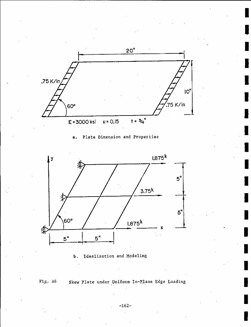
y
Fi_g. A6
·2011
E =3000 ksi u = 0.15
a. Plate Dimension and Properties
5"
X
5" .! b. Idealization and Modeling
Skew Plate under _Uniform In-Plane Edge Loading
-162-
I I I I I I I I I I I I I I I I I I I

I I I I I I I I I I I I I I I I. I I I
y
y
Fig. A7
~=lOOK
60'
E = 432,000 KSF .. = .15 t = 1.0
Discretization To Triangular Elements
(CST)
Discretization To Parallelo<;ram Elements
(Q8DII)
X
Skew Plate Under In-Plane Concentrated Loads
-163-

I 0.6 d 4d I
I d I
A 8 I 2d ' d 1- d
1-!~ I __ , ... ·I· . I ..
.. _ ..
-..,~ a. Structure and Loading I I I I I
b. 2 x 5 Discretization
I I I I I
c. 4 x 5 Discretization
Fig. A8 Simply Supported Beam with Inclined Faces I
-164- I I

I.
I I I I I I ··4,
I I
·.I I I I I 1-I
, _I
I ·I.
_ _,..... ____ X, U
Bx
z,w
y
Mxy--. .... :4.....--
,
/ y ...... . ;, '
M~+"{}Myx \
·. \ \.
z
a. Displacements
Mid-Plane Reference su·rfoce
~Ox+ dQx
b. Stress Resultants
Fig. A~ Plate Bending Stresses and Displacements
-165- .

-·.
I
y I I I · (x3 'Y3)
02 a· I
I
bl . I b2 I
Cx2, Y2) I .. ·.
03 I
ex, ,yJ) X I Fig. AlO Projected Dimensions I
I I I I
' I '
I .......
I Fig. All Intrinsic Dimensions I
-166- I I
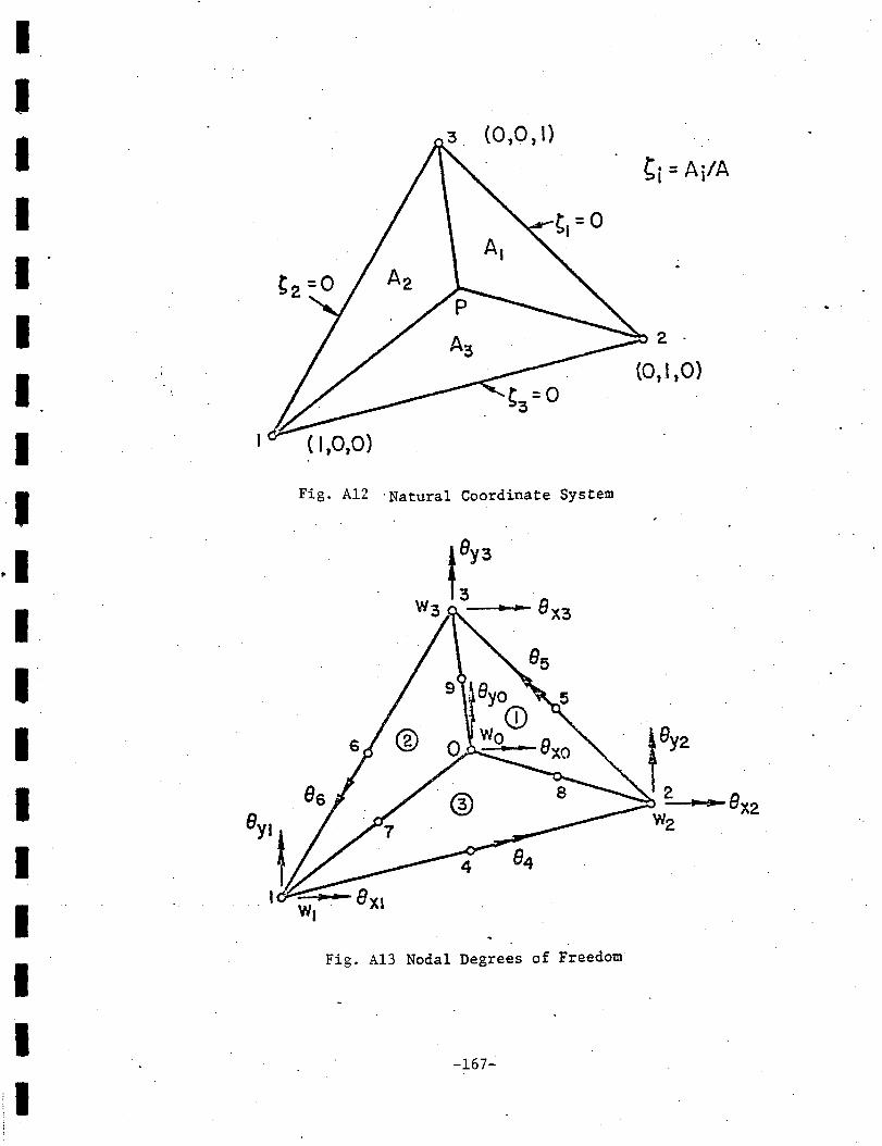
I I I
(0,0,1)
~i = Aj/A
I I. I 2 '
I (0,1,0)
I I
Fig. Al2 ·Natural Coordinate System
~I t:Y3 w3 .. ..- Bx3
I I.
I ry2 I 2
tr:!lr Bx2 Wz
I I I
Fig. Al3 Nodal Degrees of Freedom
I -167-
I I I .

!Byo r (j)
0 ...... Bxo •. ,
{~)
{I)
Fig. Al4 Subelement Displacement Components
3
Fig. Al5 Asse~bled T=iangular Ele~ents
-168-
I I I I I I I I I I I I I I I I I I I

I I I I I I I I I I I I I I I I I I I
b
I • a . i
a) a
Support On All Sides
-t
Support On 4 Sides
0 .. ,
Simple Supports On 2 Sides
Lq,
.I Simp~e Supports 2 Sides
/
' .i
Case I Concentrated load at center Fixed supports
Case 2 Concentrated load at ceter Simply supported
Case 3 Uniform load, simply supported
Uniform load
Skew angle 9 varied
Case I Uniform load Skew angle cp varied
Case 2 Concentrated load at center
. cp = 45°
Case Uniform load cp = 30°, b/Lcp = 0.40
Case 2 Concentrated load cp = 30° , bllcp = 0.40
Case 3 Uniform load b/Lcp = 0.5,4;> varied
Fig. Al6 Numerical Examples and CompaFisons for Plate · · Loading
-169-

I
I a I
I I
I- 0 -----+. o. Square Plate· b. 2x2
,,
1 l I
I
I I
; !
I
I •
~-~---r- -- .....__ -
· c. 4x4 d. 8x8
l I I I j
I
I
I I
I ~ .. _ ..... _ -- •
T -·-· I
T_ • ...__- -
e. IOxiO f. 16x 16
·'Fig. 'Ai7 Fully Supported Square Plate and Discretizations
-170-
I I I I I I I I I I I I I I I I I I I

-------------------
I t-' -....! t-' I
---WK
~ _ .,~ ... ~CM 1- :· / " ---- p
~ I~ - / '"''-- ------ Q -19
20 --- ACM From Ref. 58
--M
-----...1 --------.<{ 1 -- - 300 400 ~ 0~~------~------~~========~=======3~~~~~~ ~ ; 100 ------ 200
z -----t p --~ ........ ----- __ __,_.,....,.. 0:: -10 0 0:: 0:: w ~ 0
20
Fig. Al8
I
I I
/M
NUMBER OF DEGREES OF FREEDOM
Percent Error in Central Deflection Versus Number of Degrees of Freedom -Fixed Supports with Concentrated Load at_ Center

I 1:-' "'-J N I
0/ 0 ERROR IN CENTRAL DEFLECTION
20
10
-to
-20
Fig. Al9 .
NUMBER OF DEGREES OF FREEDOM
Percent. Error in Central Deflection Versus Number of Degrees of Freedom -Simple Supports with Concentrated Load. at Center.
-------------------


I I
0 Finite Difference (Ref. 37) I 4.0 A Fini1e Element I 0
~ v=0.3 0
I 0"
X
LU ._ 0 I <t
.J 3.0 0.
w I :I: b ._
LL. I 0
0:: y w I ._
z w u
~ I z 0 I -._ (.) w .J I LL. w -vij 0
It) I I 0
I 30 15 75 60 45
SKEW ANGLE cp I I
Fig. A21 Deflection at the Center of a Simply Supported I Rhombic Plate - Uniform Load ·
-174- I I

I I.
I t-a
5
I C\1 I
Q
I )(
C\1
l- . I 0 0" a
I )(
w t-
I <t
~.,. ...J Cl.
I w :X: t-Lr..
I 0
0:: w
I. t-z w (.)
I t-<t
I ::E t-z
I w
Finite Difference (Ref. 37) ~ 0 0
D. Finite Element ::E
I .. 71 = 0.3 . . .. ·-·- ..... _
\ l .
I. 90 75 60 45 30 15
I SKEW ANGLE <P
Fig. A22 Principal Moment Hp at Center o_f a Simply
I Supported-Rhombic late~ Uniform Load
I -175-
I

(\J -II
lO . @ co
y
Support Line
E = 30,000 ksi
71 = 0.30 t = 0.25
X
12"
16.97"
I ~ @2.12111 = 16.97
11
·· ...
1
Fig. A23 Skew Steel Plate, Two Sides Simply Supported -Concentrated Load at Center
-176-
I I I I I I I I I I I I I I I I I I I

- - - - - - - - - - - - - -· - - - - -
I 1-' ....... ....... I
...
'~~~----~~--~-----1~ \ pcf> /2-· ----:o--.. --~----------~-,~~L-~----------------~~--;
E = 1.0665 x 10⁶ lb/in2
v = 0.215
·t = 3.47 b= 40.0 in ·
ic~> = 100 in ~ = 60°·
ix = 86.66 in
Fig._ A24 Skew Slab Model (Ref. 4S) and Discretization Scheme 1
\

... ..
. Discretization Scheme 2
Discre1ization Scheme 3 Fig. _A2~ Skew Slab Model Discretization Schemes 2 and 3
-------------------

I I I I I I I I I I I I I I I I I I I
--- -- -
0
)()
en 2 0 ~ (.) w ..J ll.. w 0
0::: w
o Finite Difference (Ref. 55) A Finite Element
b/L¢ = 0.5
y = 0.2
Lcp ... I
Supports
·~
z 0.1 w (.)
oL-~~~~~--~~--~~----~----. 9Q. 75 60 45 30 15
SKEW ANGLE ¢
Fig. A26 Deflection of a Skew Plate, Two sides Simply Supported - Uniform Loads
-179-
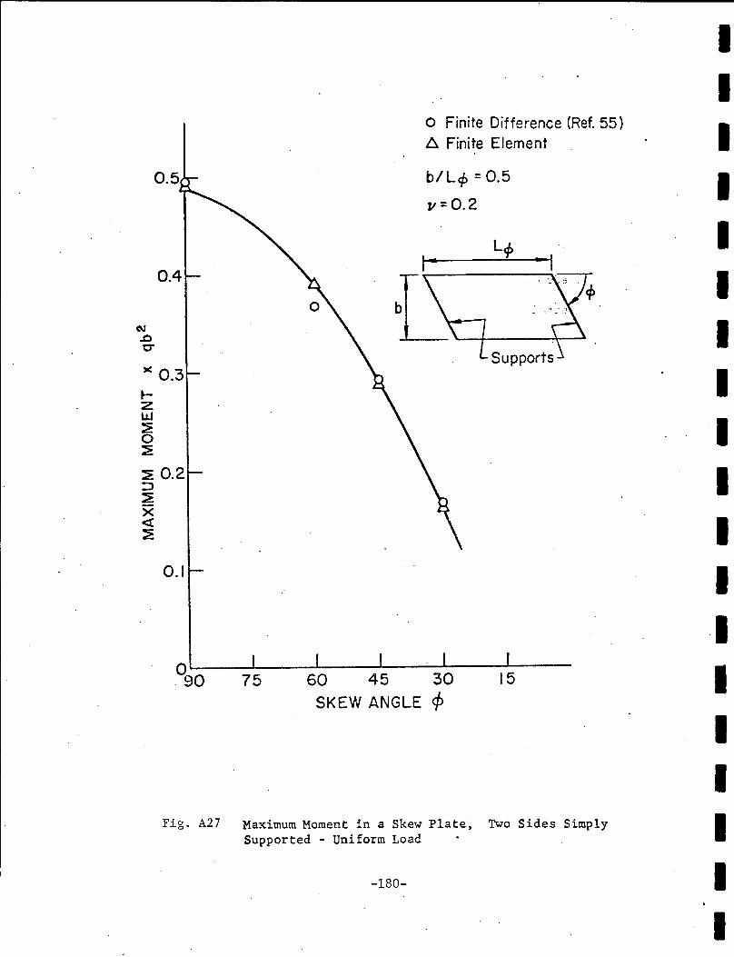
I I
o Finite Difference (Ref. 55)
I b. Finite Element
b/Lcp = 0.5 I y=0.2
L<t> I 0.4 I
c.\1 I .c cr
)( 0.3 Supports
I t-z w
I ~ 0 ~
::E 0.2 I ::::> ::E X <t I ::E
0.1 I I
090 I 75 60 45 30 15
SKEW ANGLE cp
I I
Fig. A27 Maximum Moment in a Skew Plate, Two Sides Simply I Supported - Uniform Load
-180- I I

I I I I I I I I I I I I I I I I I I I
APPENDIX Al
Q8Sll ELEMENT STIFFNESS MATRIX
The Q8Dll element approximates the in-plane behavior of
the deck slab in this study. This element has 10 fundamental degrees •
of freegom and one generalized coordinate ~ describing the constant •
shear ·.strain throughout the. element. The derivation follows the . -,
derivat~on of the element Q8D9 in Ref. 59.
The relationship between the natural system of coordinate
and the global right cartesian coordinate system is expressed by:
:} 0 x. l.
(A.36) = 0
The assumed displacement function is a linear shape function
for the corner points and a quadratic function for the internal
node:
u.· l.
u ~ 0 ~ 0 v. l 2 l. = (A. 37)
v 0 ~ 0 ~ uo 1 2
v 0
where 1
,,.)(1 + Tl'Tl·) t =- (1 + 1 2 1 1
2 2
i = (1 .. ' )(1 · .. Tl ) 2
-181-

A. 37 by
The displacement gradient field can be derived from Eq.
appropriate differentiation.
I 0~ o92 --l. 0 0 u.
ox ox l.
0~ o\ v.
l.
[Vv} = 0 _,.l. 0 (A. 38) oy oY u
0
o~. 0~1. 0~ 0~ v l a :a 0
oy ox oy Ox
Equation A.38 can be rewritten in the form
[Vv}. = [V~]
v. l.
u 0
.v 0
(A. 38a) ·
The strain field, by assuming constant strain throughout
the element, can be written as:
0~ 0 _l..
ax e:x
o~· 1
e:y 0 dy
Yxy b 0
ot _a Ox
0
0
-182-
0
\
ot a
0
0
0
1
u. l.
u 0
v 0
(A.39)
I I I I I I I I I I I I I I I I I I I

I I I I I I I I I I I I I I I I I I I
Equation A.39 can be rewritten into the form
u. 1.
E:x 1 v. 1.
<y / = [•. J u
0
Yxy v
0
(A. 39a)
Ct
With the use of the Hu-Washizu variational principle,
William has shown in Ref. 59 that the stiffness relationship is
of the form
where for this element:
~}T = (F . Ul.
=
0 k ve
k. -k ev ee
F • Vl.
v. 1.
F . uo
u 0
v } 0
v
e
= Yxy strain degree of freedom
and the individual submatrices are defined as:
[k J = [k JT = I[~ ][D](V~] dV ev ve e
[k J ·=I [2 ](D][~ ] dV ee e e
-183-
(A. 40)
(A. 40a)
(A.40b)
(A. 40c)
(A.40d)
(A. 40e)

The submatrices are evaluated by numerical' integration
described in Section A. 2. 3. The strain degree of freedom is elimin-
ated by static condensation procedure as described in Refs. 17 and 18
~esulting in the following final form of the element stiffness.
[k] = [k ]T [k ]-l [k ] (A.41) ev ee ev
-184-I
I I I I I I I I I I I I I I I I I I I

I I I I I I I I I I I I I I I I I I 1-
APPENDIX A2
COMPATIBLE DISPLACEMENT FUNCTIONS FOR PLATE BENDING ELEMENT Q-19
This appendix contains the displacement functions for the
quadrilateral element Q-19 given by Eq. A.29. The following is
taken from Ref. 17 and reproduced here for completeness.
The displacement function for sub-element 3 in Eq. A.29
is expressed by
(A. 42)
where .
{;(3)..=i(3)i (3)~ (3)~(3) 2 (3)~ (3)~(3)t (a)~ (a)~ (3)~(3)~(3)
-J l4 9xl 9yl W2 9X4 9Y2 -.:13 exa 9y3 94 9s 96
(A. 43)
and the individual functions are given by the following equations in
terms of the dimensions of the complete element:
2 .
= (_ (3 - 2' ) + 6~ ' ' ' "'l 1 3123
3
+ ' [3(A -~ )' +(2~ -A )' -3~ ' ] 3 a 3 1 3 2 3 3 2
a 1 2
= ' (b2 ' -b ' ) + (b -b ~ )' ' ' + -6c [3(b A 1 3 3 2 1 3 3 l 2 a 3 2 2
+ b ~ -2b )' +3(b ~ -b )C +(3b -b A -2b ~ )'] 3 3 1 1 3 3 1 2 1 2 2 3 3 3
~) 2 a t = ' (3 - 2' ) + 6A ' ' '+ ' (3(~ -A )' wa 2 a 3 1 2 3 a l 3 2
+(2A -~ )' -3A ' ] 3 l 3 3 l
-185-

- b A -b ~ )' +3(b -b A)' +(-3b -b ~ +2b A)' ] 3 3 1 1 2 2 3 3 1 2 1 1 3 3 3
(3) 2 ~ ev~ = ..!
6 ' [3(3b +b +b A)' +(b ~ -b A)' -3(b +3b +b ~ )' ]
~ 3 1 a 1 1 a a a 1 1 3 1 a a 2 l
(3) 4A 2 ~8A = 3L [6, ' ' + ' (5, - 3)] .. 123 3' 3
3
( 3 ) 4A i =-e 3L
6 1
2
[' (3, ' ) ] 3 2 3
(3) 4A a ~ = - [' (3, - ' ) ] 84 3L 3 1 3
3
For iSyi, all the b' s· in t 6~i are changed to a's.
For sub-elements 1 and 2, all superscripts and subscripts
permit cyclically from 1-2-3 to 2-3-1 to 3-1-2 an·d from 4-5-6 to
5-6-4 to 6-4-5.
-186-
I I I I I I I I I I I I I I I I I I ·I

I I I I I I I I I I I I I I I I I I I
APPENDIX B
FINITE ELEMENT ANALYSIS OF SKEWED STIFFENED PLATES
B.l General
The type of structure discussed in this appendix is illustrated
in Fig. 4. The plate or deck in this case can have arbitrary boundaries
and the stiffeners or the beams can be eccentrically or concentrically
attached to the deck.
When the stiffeners are eccentrically attached to the plate,
the bending of the stiffeners causes in-plane deformations in the plate
in addition to the plate bending deformations. These in-plane defor-
mations are normally not considered in classical plate theory. In
the finite element method of analysis, the in-plane and out-of-plane
behavior can easily be represented with the use of in-plane and plate
bending elements.
The in-plane and out-of-plane plate elements have been pre-
viously discussed. In this appendix, the stiffener element is de-
scribed. Since the plane of reference for the plate elements has been
defined at the midplane of the plate, the behavior of the stiffener or
beam element is also defined about this plane.
Five displacement components are selected at each node in the
present finite element approach. These are the displacement u, v, and
w in the x, y and z directions respectively, and two slopes 9 and 9 X y
about the x andy axis respectively (Fig. Bl).
-187-

I B.2 Derivation of the Beam Element Stiffness Matrix I
The stiffener element with the plane of reference as the I middle plane of the plate is shown in Fig. Bl. It is assumed that the
stiffener is attached to the plate along the boundary of a plate ele- I ment. It is further assumed that external loads are applied only to
the plate elements or directly at the nodes. Bending about the z-axis I is neglected. I
In order to satisfy compatibility of displacement along the
I juncture of the plate and the stiffener elements, the displacement
functions of the plate along the juncture must be the same as for the I stiffener element. Since the assumed in-plane behavior of the plate
is linear and the out-of-plane behavior is cubic, a linear displacement I functions is assumed for the in-plane behavior of the beam, and a cubic
I displacement function is assumed for the out-of-plane behavior of the
beam. Furthermore, since the normal slope of the plate is assumed to I vary linearly along the boundary, the twist of the beam along this
boundary is assumed to be linear. I The geometry of the beam element can be described in terms of I
non-dimensional coordinates:
s L - X (B.la) = 1 L
I X (B.lb) s =-
2 L I
where L is in the direction of the x-axis. I I
-188- I I

I I I I I I I ·I I I I I I I I I I I I
The linear displacement function for u.and the cubic dis-
placement function for w can then be written as
u = a l; I;; l; l l 2 2
(B. 2)
2
w = a 1;3 a 1;3 a l; 1;2 a l; 1; (B. 3) 3 l '+ 2 5 1 2 6 1 2
In matrix notation:
u 1';1 ·0 0 0 0
= (B. 4)
w 0 0
T a } where {a} = {a a a a a 1 2 3 '+ 5 6
The coefficients a and a can be determined from the two in-1 2
plane model displacements at the two nodes, and a a a , and a can 3 '+ 5 6
be determined from the two out-of-plane displacements and two rotations
at the two nodes.
The nodal displacements can be written as,
(B. 5)
where ui and ~ are the in-plane displacements, and wi, wk, 9yi' and
Oyk are the out-of-plane displacements and rotations, at nodes i and k
respectively.
chain rule,
9 can be expressed by definition and the use of the y
(B. 6)
-189-

The nodal displacements can now be expressed in terms of the
unknown coefficients from Eqs. B.4 and B.6.
ui 1 0 0 0 0 0 a. 1
wi 0 0 1 0 .0 0 a 2
eyi 0 0 -3/L 0 1/L 0 a. 3
= (B. 7)
~ 0 1 0 0 0. 0 a It
wk 0 0 0 1 0 0 a 5
eyk 0 0 0 3/L 0 :...1/L (X 6
The vector of unknown coefficients can be expressed in terms
of the nodal displacements by solving for {a} in Eq. B.7. Hence,
a 1 0 0 0 0 0 u. 1
~
a. 0 0 0 1 0 0 w. 2
~
a 0 1. 0 0 0 0 6 yi 3 (B. 8)
= a 0 0 0 0 1 0 uk
4
a 0 3 L 0 0 0 wk 5
a. 0 0 0 0 3 -L eyk 6
-190-
I I I I I I I I I I I I I
I I I I
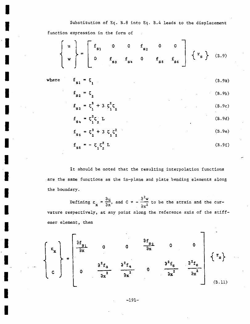
I I I I I I I I I I I I I I I I I I I
Substitution of Eq. B.8 into Eq. B.4 leads to the displacement
function expression in the form of
u
= w
where f 51
f 52
f 53
f 54
f ss
f s&
=
=
=
=
l;1
l; 2
l;3 1
f Sl
0
0
f 53
+ 3 r,;2z; : 1 2
l;2.l; L 1 2.
= l;3 + 3 l; l;2. 2 1 2
=- z; z;2. L 1 2
0
f sa.
f 52
0
0
f ss
0
f 56
{ rs} (B.9)
(B. 9a)
(B.9b)
(B. 9c)
(B. 9d)
(B. 9e)
(B. 9f)
It should be noted that the resulting interpolation functions
are the same functions as the in-plane and plate bending elements along
the boundary.
du a2w
Defining E = -- and C = - --- to be the strain and the cur-x ax' ax2
vature respectively, at any point along the reference axis of the stiff-
ener element, then
"x ~ 3£ 3£ _2L 0 0
_ll 0 0 ax ax
= { rs} 2. 32.£4 32.£ 32.£
c J a. £3 6 s
0 0 ax2 3x
1 3x2 3x
2
(B .11)
-191-
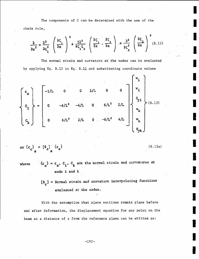
The components of C can be determined with the use of the
chain rule,
( ~·) 2
za 2
ax + az;; z; 1 2
2
( ~) (B.l2)
The normal strain and curvature at the nodes can be evaluated
by applying Eq. B.l2 to Eq. B.ll and substituting coordinate values
e: X
ci
where
u. l.
-1/1 0 0 1/1 0 0 w.
l.
eyi (B .13)
= 0 -6/12 -4/1 0 6/12 2/1
~
0 6/12 2/1 0 -6/12 4/1 wk
eyk
= [~ ] . {r } c s s
(B .13a)
· {e:c} = e:x' c1
, Ck are the normal strain and curvatures at
node i and k
[~ ] = Normal strain and curvature interpolating functions c
evaluated at the nodes.
With the assumption that plane sections remain plane before
and after deformation, the displacement equation for any point on the
beam at a distance of z from the reference plane can be written as:
-192-
I I I I I I I I I I I I I I I I I I I

I I II I "I-
I I I I I I I I I I I I I
U(z) = u - z. aw ax (B .14)
The normal strain e: can be defined by differentiating Eq. X
B.l4, from which the stress-strain relation for the beam becomes
(B .15)
where cr = stress on a stiffener element at· distance z from the s
reference axis
E = is the modulus of elasticity of the beam s
assuming only a uniaxial state of stress for the beam.
The generalized forces acting on the beam section can be
evaluated by integrating Eq. B.l5,
N ... ft/2
s -i:/2
M !t/2 s = -t/2
(J dA s
(J z dA s
(B .16)
(B.l7)
These generalized forces can then be expresse~ in matrix form as,
A s 3u N ax s s s
= E (B .18) s
s I . a~
M --s s s 2 ax
-193-

where A = cross-sectional area of the stiffener s
S = first moment of the stiffener area with respect to s
the plane of reference
I = moment of inertia of the stiffener area with respect s
to the plane of reference
Given the normal strain and curvatures at the nodes as
expressed by Eq. B.l3, the strain and curvature expressions can be
written in terms of strain interpolation functions. Thus
au 1 0 0 € ax X
= ci (B .19)
a2w 0 l;l l; ck ---
ax2 2
or {E}s = [~€] . {Ec} s s
(B. 20)
where {e:} normal strain du and <iw the = and curvature ax ---along
s dx2
axis of the beam element about the reference plane
[<I>e:]s = strain interpolation functions which express a con-
stant variation of normal strain and a linear vari-
ation of curvature
{e: } = normal strain e: and curvature C at the nodes c s X
The specific characteristics for the beam element can be
expressed from Eq. B.l8 to be,
.(D) s :: J (B. 21)
which are already integrated for the complete beam section,
-194-
I I I I I I I I I I I I I I I I I I I
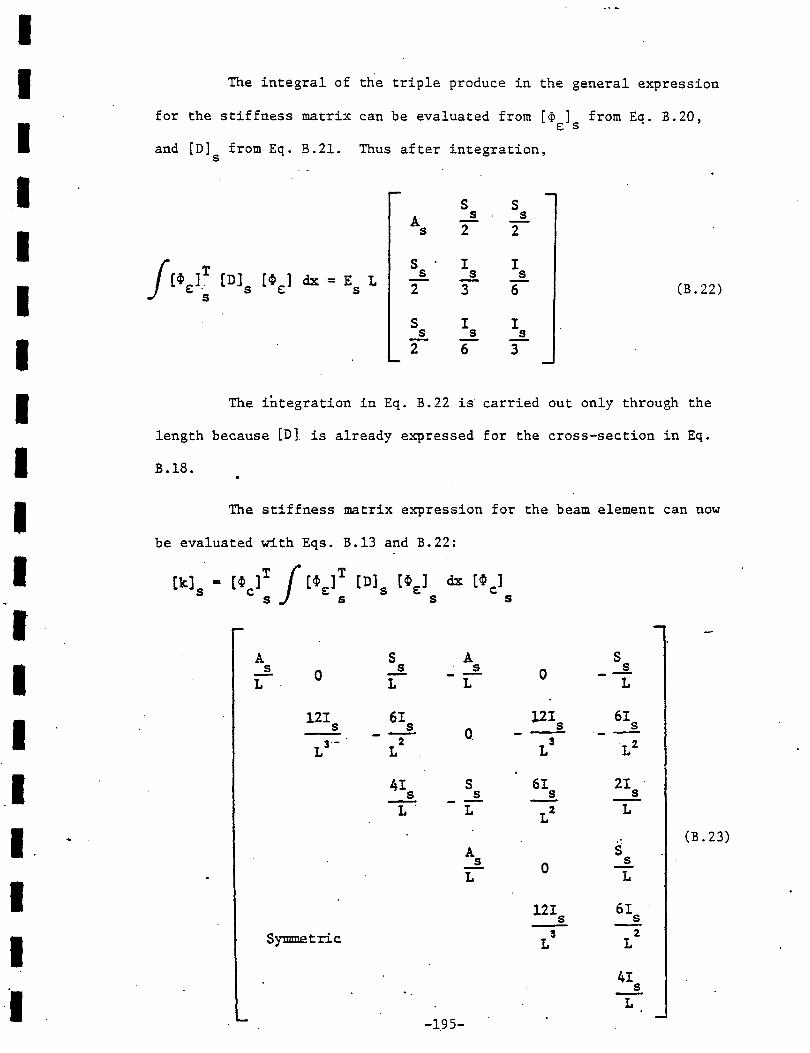
I I I I I I I I I I I I I I I I I I ··I
The integral of the triple produce in the general expression
for the stiffness matrix can be evaluated from [~E]S from Eq. B.20,
and [D] from Eq. B.21. Thus after integration, s
s s A ....!. S.
s 2 2
J[~ ]T [D] s . I I
(~ e:] dx E L s s s = e: . s s 2 3 6 (B.22) s
s I I s s s 2 6 3
The integration in Eq. B.22 is carried out only through the
length because [Dl is already expressed for the cross-section in Eq.
B.l8.
The stiffness matrix expression for the beam element can now
be evaluated with Eqs. B.l3 and B.22:
dx [~ ] c: s
A s A s ....§.. 0 ....!. s 0
s -- --L L L L
121 6I l2I 6I s s
0. s s -- -- ·--3- 2. L3 . 1
L L L
4I s 6I 2I s s ~ s - --L. L L2 L
(B.23) A s
s 0 s
L L
12I 6I s s
Symmetric: ! 2 L L
4I s L
-1.95-

It should be noted that the above expression is only for the
bending stiffness of the beam. The torsional stiffness is derived
separately in the following paragraphs.
For the present analysis, only St. Venant torsion is con-
sidered. It ·has been shown that for rectangular and stocky beam cross-
sections, most of the applied twisting moment is resisted by St. Venant
torsion (Ref. 58).
The twisting moment T in the beam element is related to s.v.
the angle of twist <P by the· relation:
where
'I =GK ¢' s.v. t
(B. 24)
<P 1 = ~x ( ~; ) or the rate of change of angle of ·twist
G = shear modulus
K = St. Venant torsional constant t
With the assumption that the angle of twist varies linearly
along ~he length of the element, and recognizing that the angle of
twist at the nodes corresponds to the rotation about the longitudinal
axis of the beam, the torsional rotation function can be written in
terms of linear interpolation functions and the nodal rotations. Thus
e xi
. {¢} = [z; z; ] (B.25) 1 2 e . yl.
-196-
I I I I I I I I I I I I I I I I I I I

I I I I I I I
I I
-I
I .I I I
{¢ '} = [ - i ~ J (B.26)
Following the procedure for the beam bending element: and
using the given rotation function, the following matrices· can:·b~
defined: [D]t = Gkt (B. 27)
[~f) = [1] (B. 28) . t
[~ ] [- ~ 1 ] = . (B.29) c t L
From the general expression for the stiffness matrix, integration
.long the length leads to
= [<P ]T f [<P ]Tt [D] [<P ]t dx (<P ]t c t € ' € . c
-~~t - 1 - 1
=--L
1 1 -
B.3 Assembly of the System Stiffness Matrix . ·..:··
• 'Ihe stiffness matrices of the individual elements are assem-
bled to form the structural stiffness matrix of the complete system.
The procedure is described in detail in Ref. 64. In the following,
the assembly of the elements is illustrated in matrix form to show the
-197-

interaction of individual elements as defined by the global force and
displacement vectors.
The in-plane and bending plate elements are assembled first
to form a· combined element with five degrees of freedom at each node.
Since the in-plane plate element and out-of-plane plate element both
lie on th~-same reference plane, there is no interaction between them.
Hence, for example
k1 I o l ---;---:----I
o I krr I
(B. 31)
where k1
is a 2 x 2 matrix associated with u and v displacement compo
nents and k!I is a 3 X 3 matrix associated with theW, eX, eX displace-
ment and rotation components.
For the whole plate element with nodes 1, 2, 3 and 4,
t· f . "" ' .!;. I
' .. :, i .::-; .. ~
' - '·:. f
F 1
F 2
F 3
F It
r 1
r
(B. 32) = [kij] 2
r 3
r It
where.the submatrices of [k .. ] are in the form of Eq. B.31, and l.J
w. l.
for i = 1, 2; 3, or 4.
-198-
M .} Yl. (B. 33)
(B. 34)
I I I I I I I I I I I I I I I I I I I
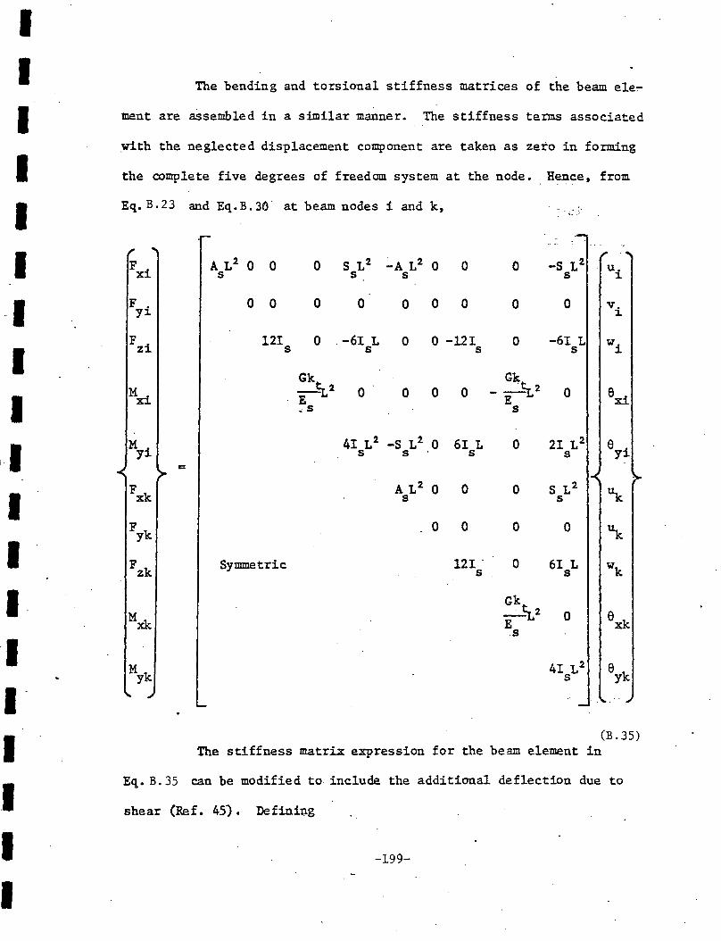
I I I I I I
·I I I il I I I ·I I I .I I I
The bending and torsional stiffness matrices of the beam ele~
ment are aSsembled in a similar manner. The stiffness terms associated
.with the neglected displacement component are taken as zero in forming
the complete five degrees of freedom system at the node •. H~ce, from
Eq. B.23 and Eq.B.30 at beam nodes i and k, . ,: _.._:
Fxi A L2 0 0 0 S L2 ._A L2 0 0 0 -s L2 u. s s s s :1.
F . 0 0 0 0 Y:L
0 0 0 0 0 vi
Fzi 121 0 -61 L 0 0 -121 0 -61 L w. s s s s :1.
Gk . Gk Mxi -~2 0 0 0 0 -~~2 0 exi E E .. s s
Myi 41 L2 -s L2 0 61 L 0 21 L2 e yi s s s s =
Fxk A L2 0 0 0 S L2 ~ s s
Fyk 0 0 0 0 ~
Fzk Symmetric 121. 0 61 L wk s s
Mxk Gk~2 E
0 exk s
Myk 41 L2 eyk s
(B. 35) The stiffness matrix expression for the beam element in
Eq. B. 35 can be modified to include the additional deflection due to
shear (Ref. 45). Defini~g
-199-
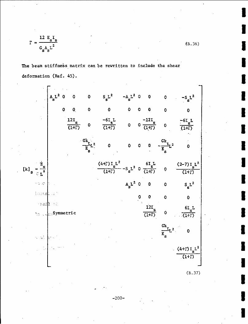
12 E I r = ---=S;__;;_S
G A L2 s s
The beam stiffness matrix can be rewritten to include the shear
deformation (Ref. 45).
. E
[k] = -i-s CL .
'.-...... -·- ···~ .
·~ .. J..
A L2 s 0 0
0 0
12I s (l+r)
0
.o
0
· Gk ·. ---::-42 E ...
s
0
-6I L s (l+r)
0
-A L2 s
0
0
0
-200-
0 0 0
0 0 0
-121 s
0 (l,:l"f) 0
0 0 Gk --~2
E s
~B.36)
0
-6I L - s _(l+r)
0
I I I I I I I I I I I I I I I I I I I

I I I I I.
I I I I I I I I I I I I I I.
The beam stiffness matrix is given for the beam element whose
longitudinal a.'<:is is parallel to the x-axis. When the beam elements
are not parallel to the x-axis, standard tensor transformation must be
applied to the beam stiffness matrix before assembly into t~ struc
tural system (Ref. 64).
The displacements of the plate and beam elements at common
nodes are expressed by Eq. B. 32 and Eq. B. 35 in terms of the global
degrees of freedom. The elements have equal number of degrees of free-
dom at the nodes and therefore can be assembled directly to the system
stiffness matrix following the procedure specified in Ref. 64.
B.4 ~pplication of Boundary Conditions
One of the advantages of the finite element method of analy--
sis is its adaptability to solutions of problems with various bound~ry
conditions. If a degree of freedom at the boundary is fixed, th~ cor-!
responding row and column of the stiffness matrix is easily eliminated l
from the solution procedure. If the support at the boundary is f~ex-
ible, the stiffness of the support is simply added to the stiffness of
the element at that boundary· (Ref. _65).
In certain cases, the nodes are constrained to displace in a
specified direction, and to rotate at a specified angle. For example,
the u displacement of a node may be specified to displace in the direc-
tion of a line at an angle w from the x-axis and the 6 rotation ~y be X
specified to rotate about a line at an angle S from the x-axis. For
-201-

these cases, the stiffness matrix mu-st be transformed accordingly. It
is shown in Ref. 64 that the required transformatio-:1 is of the form
[k'] = [T]T [k] [T] (B. 38)
where [k'] = the transformed stiffness matrix
·[k] = the original stiffness matrix
[T] = the transformation matrix
It should be noted that the transformation can be carried out in the
element·stiffness level [k] or at the assembled system. stiffness matrix
[K]. It should be noted further that the applied nodal forces and the
·resulting deformations are in the direction specified by the constraint.
For the five degree of freedom system in this study, the
transformation matrix for a given node is
.•:: ·~ :~ _1: cos w sin w 0 0 0
:'l··-=· J . . :· -sin w cos w 0 0 0
r~0.L: (T)= 0 0 1 0 -o (B. 39)"
.> :·:,i ;::-~ 2· ~· 0 0 0 -cos 6 sin e .-?:j'j· ... ,.
where
0 0 0 -sin (! cos e
w = the angle from the global x-axis along which u displaces,
measured clockwise; and
e = the angle from the global x-axis about which e rotates' X
measured clockwise.
-202-
··---- - -- --· ·-·---------· -···-·-- .. -·---·
I I I I I I I I I I I I I I I I
. - ~ ·· ....
I I I

I I I I I I I I I
·I I I I I I I I I I.
:B:-5 Application of Loads
The components of the force vector as defined by Eq. B.33 are
applied at the nodes in the direction of the associated displacements.
' For uniformly distributed loads, the force vector can be computed from
(Ref. 17).
' ~; . '... , . ~ ... (B. 40)
The uniform load is conveniently equated to a set of concentiated
forces and moments applied at the nodes. For concentrated loads, th~.
discretization ·can be made such that the load will be directly: .. op _a_ -~
node; and hence the loads can be applied directly to the global force
vector. However, the procedure of changing the discretization to ac7 .. . .. . 1' .~ :,- .
commodate concentrated loads is obviously inefficient especially for
the analysis of one structure under.different types of loading. For ·, ;~· ....
this reason, the concept of a statically equivalent force vector for a
concentrated load is introduced. In this concept, the element with a
concentrated load is analyzed as a substructure, _and the reaction
forces at the nodes are computed. The negative of these reaction ........ _Q
forces at! the nodes become the applied nodal forces for cthe assemled f)
structure: In this study only the concentrated load normal to the
plate element is considered.
·i I ,•:
The stiffness equation for the Q-19 element gives the force
displaceme~t relationships of a quadrilateral element with the fifth
node at the center of the element. If the fifth node is located at the
point where the concentrated load is applied, the resulting structure
--
-203-

'
is a quadrilateral plate of four triangles with a concentrated load at
the interior nod~ (Fig. B2). The stiffness of the four triangles can
be recomputed and reassembled in the form:
0
= (B. 4-J,)
where 0 refers to the supported nodes and, where the subscripts E and I
refer to the external nodes and the internal node respectively. The
external nodes in this case are completely fixed in displacements and
rotations •. {FE} can therefore be easily found to be
.:(B. 42)
Since Eq. B. 41 is an equilibrium equation,· {FE} is a stati
cally equivalent force vector. In cases however when the concentrated
load is very near to a corner node of the quadrilateral, the stiffness
formulation may get into numerical difficulty because of the resulting
shape of one or more of the triangular elements. In such. cases, the
.concentrated load is applied directly to the nearest node. When the
concentrated load is on the boundary of the element but not on the
node, the load is proportioned to the two nodes of 'that boundary. The
components of the equivalent force vector due to a concentrated load
normal to a quadrilateral element a'.l'!'e illustrated· in Fig. 132.
-204-
I I I I I I I I I I I I I I I I I I I

I I I I I I I I I
:·I. I I I I I I I I I
. / y
d
·.::..
Fig. Bl
{ x,y) =Plane of Reference
z
., j
A·stiffener Finite Element with Associated Degrees of Freedom and Nodal Forces
-205-
~.. '
.~; . . ...
.. ' . ~} .
,; .::~ . '. :~ ·'1 :. '
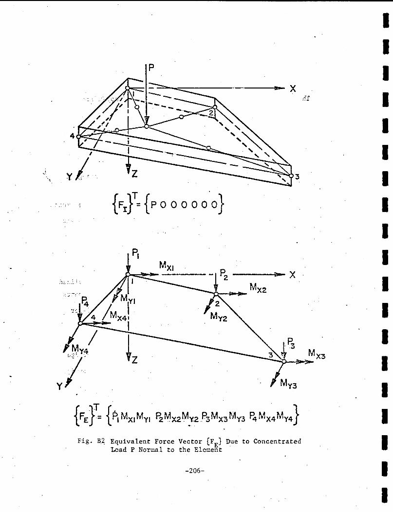
·.
p
I
v/ ..... -·· l,~ .. •
Fig. B~ Equivalent Force Vector [FE] Due to Concentrated Lead P Nor~l to the Element
-206-
rf[
I I I I I I I I I I I I I I I I I I I

I I I I I I I I I
.I I I I I I I .1 I I.
iO. NOMEN CIA TURE -·:···· ·,
. ','"" The following symbols were used in the text ~~~~~ndices:
~ \ ',,""' Capital Latin Letters (matrices and scalars) ' · ~.,- . A.
(A]
A
A. l.
A s
[:s]
c
C ,C ,C ,C ll 12 21 33
(D]
(D] _S
D. F.
.. -~ . '···
E, E , E 1 2
E s
{F J e
\ ·. \ ... ··~ .,.,
= Matrix of displacement ~functi<?.ri:s' '
evaluated at the nodes _ ~-:-~;.;~.~ · .,i ,1 '.
= Area of a triangular element \ ·~,
= Area of sub element i in a triang1.,1lar
element
= Cross section area of stiffener element
= Matrix of differentiated displacement
functions
= Curvature in a stiffener element
= Material constants
= Elasticity matrix relating generalized
stresses to generalized displac~ments 1 _ ..
= Elasticity matrix for the stifferter ·-- .. ---~
element -· -~-~
= Distribution factor -. -.-M ·;~
= Distribution factor in a skew bridge '
= Distribution factor in a right bridge
= General and principal modulus of
elasticity 'i. 5
= Stiffener', element modulus of ·. ··- ... ,_ ·.
-- J elasticity
= Statically equivalent force vector due
to di~tributed loads
-207-

':··'
' {F }
F . ,F . ,F . ,M . ,M . X~ y~ Z~ X~ y~
G, G
G s
H ·'
I
I s
J ,J ,J ,J ll 12 2~ 22
[K]
[M}
M , N s s
M ,M ,M ,M ,M X y ~ .1 2
.. . J
N· ,N ·:,N· . ,N ,N x y xy 1 2
M M u' uv
= Vector of element nodal forces
= Applied force vector associated with
external nodes
= Applied force vector associated 'tvith
internal nodes
= Statically equivalent force vector
due to concentrated load
= Components of element nodal forces
{F.} ~
= General and second principal shear
moduli
= Stiffener element shear modulus
= Stiffener to slab stiffness ratio;
(~I)stiffener/(EI)slab
= Integrand expression
= Moment of inertia of stiffener element
about reference plane
= Components of Jacobian matrix
= Global stiffness matrix
= Bridge span length, stiffener element
dimension
= Matrix of displacement functions
= Generalized forces in stiffener element
= Cartesian and principal plate moments . ·'
. • : _t. . ~~; • • ..
- Carte.sian and principal in-plane
= Moment resultants in the direction of
sket;..r
-208-
I I I I I I I I I I I I I I I I I I I

I I I I I I I I I ·I I I I I I I _I
I I.
PCTR
PCTR(EXT)
PCTR(BOX)
(R]
s
s s
(T]
u, v
w c
= Percent reduction in the distribution
factor for interior I-beams
= Percent reduction in the distribution
factor for exterior I-beams
= Percent reduction in the distribution
factor for interior box-beams
= Global force vector
= B~am spacing
= First moment of the stiffener area
with respect to the reference plane
= Transformation matrix
= In-plane strain function
= In-plane displacement at distance z
from the reference plane
= Bridge curb to curb width
= Weight coefficients
,. : l.".
B. Small Latin Letters (matrices and scalars)
a, b
a. ,b. 1. 1.
d
e
.• "j
.• ,_!';~. •;.
; .=-_;_ ~~
= Web element dimensions ,. " i \~ ...
= Projected dimensions on x and y axes
= Stiffener element depth; distance from
the centroid of a truck wheel load to·
the drive wheels
= 2A/ J,i
= Eccentricity of the centroid of the
st'fff~n~t-- element cross section:::~t8 .-the
plane of reference
= In-plane displacement function
,,.
-209-

i,j,k,.t
[k]. ,·
k k k ev' ve' ee
~.:. : .-.
[k] s
[k]~
' [k J
m
n
P(x,y), q
(r}
= Stiffener element disp·lacement function
= normal distance of node i to side l. 1
= Node or sub element number
= Element stiffness matrix
= Partitioned matrices of the element
stiffness matrix associated with
external and internal nodes
·= Submatrices of the element stiffness
matrix associated with displacement
and strain formulations
= Submatrices associated with in-plane .. - .
and out-of-plane behavior
= Stiffener element stiffness matrix
= Stiffener-element stiffness matrix
for torsional behavior
= Transformed element stiffness matrix
= Length of side i in a triangular element
= Ratio of shear modulus G to elastic 2
modulus E 2
= Order of interpolation function;
principal modulus of elasticity ratio~
E /E 1 a
= Normal distance of a point i to side
l 1 in a triangular element
= D:tstri.bq:ted, load intensity
= c6nsist:ent-"force vector associated with
the displacement formulation
= Global displacement vector
-210-
I I I I I I I I I I I I I I I I I
.I I I

I I I I I I I I I I I I I I I I .I I I
{r (i)}
{r } s
{r } e
{r } 0
u,v,w
x,y,z
= Element nodal displacements
= Sub element nodal displacements
= Stiffener element nodal displacements ··
= External node displacements for plate
element
= Internal node displacements for plate
element
= Displacement components
= Components of the element nodal
displacements
= Nodal displacements at exterior nodes
.s
;_ .·:.
= Nodal displacements at interior nodes; ~ .; '· .
= Cartesian coordinates
= Cartesian coordinates of node i •. I ,,
C. Capital Greek Letters (matrices and scalars)
r = Shear deformation parameters
= Matrix of interpolation or shape
functions
·.:
... '•
= In~erpolation functions for a triangular
element in terms of the external degrees
of freedom
= Sub element i interpolation function
= Strain interpolation functions evaluated
·.at,_,;P,e :n<?des
-211-

_[i]t
[~ '] e
[i (i)] e:
[i . ] 11.
= Strain interpolation function for the
stiffener element evaluated at the
nodes
= Twist interpolation function for the
stiffener element evaluated at the
nodes
= Interpolation functions associated
with the external nodes
- Interpolation functions associated
. with the internal nodes
= Curvature interpolation functions
[ i(i)] evaluated at the nodes
= Shape functions associated with the
global nodal derivatives
= Shape· functions associated with the
local nodal derivatives
= Strain shape functions describing the
variation of strains
= Triangular sub element strain inter
polation functions describing the
variation of curvature
= Stiffener strain interpolation function
describing the va~iation of twist
= Geometric shape functions
= Linear shape function
= Quadrat~c shape function
= Linear sh~pe functions associated •. ·. ·, ~
with nodes i
-212-
I I I I I I I I I I I I I I I I I .I I

I I I I I·
I I I I ,I I I I. I I I I I I.
= Matrix relating curvature components
to nodal degrees of freedom
D. Small Greek Letters (matrices and scalars)
{a} =·Generalized coordinates
~ = Angle measured from the global x-axis
in the direction of which u displaces : ·.
e ,e XX yy
\I ;v 2
{a}
a ,a XX yy
.,. xy
\ .
,_ .
= Shear strain
= Strain .field
= Vector of nodal strains
= Normal strains
= Local coordinates
-= Non-dimensional nodal coordinates
= Rotations about the global x and y
axes
= Nodal rotations
= 1- t... 1
= Poisson's ratio
= Stress field
= Normal stresses
= Shear stresses
i .. •. l; ·.- ., .···,:
= Skew angle, angle of twist
= Interpolation functions in terms of
the nodal out-of-plane displacements
'-213-
"'
.. '
i-

w
E. Element Designation
ACM
CST
LCCT-12
LCCT-11
LSE
M
p
Q-19
Q8Dll
Q8SP12
WK
= Angle from the global x-axis about \·Jhich
e rotates X
= Local derivative at node i
= Adini, Clough and Melosh plate bending
element
= Constant strain triangle in-plane
element
= Linear curvature compatible triangle
with 12 degrees of freedom
= Linear curvature compatible triangle
with 11 degrees of freedom
= Linear strain equilateral
= Melosh plate bending element
= Pappenfuss plate bending element
= Quadrilateral plate bending element
with 19 degrees of freedom
= Basic 8 degree of freedom in-plane
element with 3 additional internal
degrees of freedom
= Basic 8 degree of freedom in-plane
element >vith 4 additional nodal
rotations
= Wegmuller and Kostem plate bending
element
-214-
I I I I I I I I I I I I I I I I I I I