I. CHAPTER 1 Using major elements to determine sources of

I. CHAPTER 1

Using major elements to determine sources of nitrate in groundwater

i. Introduction

Nitrate and urban contamination affects many aquifers, for example, in Turkey (Elhatip et

al., 2003), the UK (Barrett et al., 1999), many parts of the United States (Kolpin et al., 2002;

Lerner, 2002; Thomas, 2000; Williams et al., 1998) and Germany (Trauth and Xanthopoulos,

1997). The most cost efficient way to prevent nitrate contamination is to determine its source and

reduce it there. Previous investigators of the sources of nitrate in groundwater on Long Island

have used δ15N values of nitrate-nitrogen to identify nitrate contamination (Bleifuss et al., 2000;

Flipse and Bonner, 1985; Flipse et al., 1984; Kreitler et al., 1978). However, due to overlapping

source signatures, nitrogen isotopes alone were not sufficient to characterize the sources of

nitrate. More recent studies have shown that major elements that accompany nitrate in the

groundwater (Bleifuss et al., 2000; Elhatip et al., 2003; Trauth and Xanthopoulos, 1997) may

distinguish sources of nitrate with less ambiguity.

In this study samples of soil water collected below turfgrass that is fertilized with natural

organic fertilizer, traditional chemical fertilizer and not fertilized and samples of wastewater

from septic tank/cesspool systems and public sewage treatment plants were analyzed for major

elements. Major element data for groundwater from Suffolk County Water Authority municipal

wells (CDM, 2003) and monitoring wells from Bleifuss et al. (2000) have been characterized as

a function of land use. The data for the groundwater were compared to the wastewater and the

soil water. Binary plots of the elements Na, Mg, Ca, SO4 and N-NO3 when normalized to Cl

12

concentrations proved most successful as nitrate tracers along with binary and ternary diagrams

of Cl, SO4 and N-NO3. Normalizing the data to a conservative element1 such as Cl reduces the

effects of mixing and dilution providing a more precise evaluation of nitrate sources. Estimates

of mixing proportions from each source were calculated using a mass balance and water budget

approach.

Nitrate sources: chemical concentrations and origin

Researchers commonly contribute elevated levels of major ions in groundwater

influenced by residential areas to be from wastewaters but few have analyzed wastewater or

other urban sources. Some of these studies include (1) Renyolds (1994) who noted elevated

concentrations of Cl, NO3, Na, Ca and K in urban groundwater (2) Wayland et al. (2003) noted

elevated levels of Na, K and Cl in urban areas compared to agricultural areas (3) Bleifuss et al.

(2000) found elevated levels of Na and Cl in residential land use groundwater (4) Trauth and

Xanthopoulos (1997) found elevated SO4, K and B below urban areas and (5) Thomas (2000)

found elevated levels of Cl, Na and Ca in shallow groundwater of urban areas.

Data presented in this study show elevated concentrations in Ca, Mg and SO4 in soil

water influenced by turfgrass maintenance compared to wastewater samples and that wastewater

is enriched in K, Na, Cl, N-NO3 and PO4 compared to water influenced by turfgrass

maintenance. The following paragraphs discuss previous work to explain some of these

differences.

1 A conservative element is an element in groundwater that travels at the same rate as the groundwater flows. That is, the element is not retarded.

13

Concentrations of elements in rain water are influenced by the source of the storm. This

can be either marine or continental in origin. The total observed loadings due to all storm events

for Long Island is highest for SO4 followed by NO3, Cl and Na (Proios and Schoonen, 1994).

Rain water chemistry is strongly influenced by the oceans and acid deposition (Schoonen and

Brown, 1994). Combustion of coal and other fossil fuels increase sulfur and nitrogen inputs to

the atmosphere which in turn increases the acidity of rain. Acid rain, a recent event, is the

probable cause for high loadings of SO4 and NO3 in Long Island rain. Trends since 1955 show an

increase in the acidity of pH in rain and increases in the global emissions of sulfur and nitrogen

(Mackenzie, 1998). The high levels of SO4 in water influenced by turfgrass maintenance,

however, are mostly derived from fertilizers. Sulfur content in Scotts Turf Builder fertilizer are

8-11% sulfur. Sulfur is also present in a Lesco brand and natural organic fertilizers at lower

percentages. The Lesco brand fertilizer is sulfur coated urea form, a slow release nitrogen source.

The sulfur in the natural organic fertilizer is natural potassium sulfate. Elevated levels of Ca and

Mg in water collected below turfgrass sites are likely from the application of lime to increase soil

pH.

K, Na, Cl, N-NO3 and PO4 in wastewater come from a variety of household items used in

the kitchen, bathroom and laundry and are present in human waste. According to Medcalf and

Eddy (2003) typical fluid contributions from a house to a septic system are 26.7% from toilets,

21.8% from clothes washing, 16% from showers, 15.7% from faucets, 13.7% from leakage,

1.7% from baths, 1.4% from dishwashing and 2.2% from other sources. An average Long Island

cesspool discharges 240 gallons (900 liters) per day (Flynn et al., 1969).

14

Eleven rural households in Wisconsin were monitored in 1976 to determine source

specific wastewater use and quality (Siegrist et al., 1976). Water usage has changed from 1976 to

2003 but the relative proportions reported by Siegrist et al. (1976) agree with those of Medcalf

and Eddy (2003). Siegrist et al. (1976) found that most of the total nitrogen in wastewater is

from nonfecal toilet flushes, making up 43.5% and fecal toilet flushes were 24.6% of the

nitrogen in wastewater analyzed in his study. All toilet flushes make up 13.8% of total phosphate

concentrations. Siegrist et al. (1976) reported 2.64g N/person/day and 0.28g PO4/person/day in

nonfecal toilet flushed and 1.5g N/person/day and 0.27g PO4/person/day for fecal flushed.

The Swedish Environment Protection Agency (Beckerus et al., 1998) determined that in

1992 in Sweden the concentrations in urine are 11g N/person/day and 1g PO4/person/day and

that feces have 1.5g N/person/day and 0.5g PO4/person/day. Another Swedish study analyzed

nutrient and heavy metal concentrations in urine for the purpose of agricultural reuse from a

source separating sewage system (Jonsson et al., 1997). They found that urine had 4g N/L and

0.35g P/L. Jonsson et al. (1997) acknowledged that these values are lower than those of the

Swedish Environment Protection Agency and attributed this to the higher proportion of

vegetarians and children in their study. Some recent studies report that up to 80% of nitrogen and

around 50% of phosphate in wastewaters is from urine (Gajurel et al., 2001; Jonsson, 2001;

Larsen et al., 2001; Wilsenach and van Loosdrecht, 2003). These percentages are higher than

Siegrist et al. (1978) and Jonsson et al. (1997). The differences could be due to geographical

differences or to differences in food consumption patterns. The nitrogen balance of a mature

human body is zero, so that the nitrogen intake is equal to the excretion. A high consumption of

meat and other protein-rich products will result in a higher nitrogen concentrations in urine (Vijst

and Groot-Marcus, 1999).

15

Chloride excretions in urine and fecal matter are approximately 6g per day per person

(Medcalf and Eddy, 2003) Daily nutritional intake for the average person is 5000mg Na

(http://www.feinberg.northwestern.edu/ nutrition/fact-sheets.html). Jonsson et al. (1997) reports

an average value for urine of 1.2g Na/L and 1g K/L. Researchers have reported around 50%

(Gaillardet et al., 2001; Gajurel et al., 2001; Jonsson, 2001) and up to 90% (Larsen et al., 2001)

of the potassium in wastewater is from urine and fecal matter. There are acceptable ranges of

most elements in urine for healthy adults (Lindberg, 2004). These values range from 0.7-8.75g

Cl/person/day, 0.345-5.75g Ng/person/day and 0.975-4.68g K/person/day.

The second largest contribution of water to the septic system is from clothes washing. In

addition to the water used in the laundry load contributions will also come from the dirt on the

clothing and from the washing soaps (Ligman et al., 1974). Laundry soaps vary in components

and concentrations but according to Beckerus et al. (1998) they are made up of surfactants, pH

stabilizers, softeners/builders, bleaches, brighteners, protective colloids, preservatives, enzymes,

perfume, fillers, defoamer, corrosion inhibitors, coloring agents and color stabilizers. Among

these phosphates are used as softeners/builders. Phosphates coming from detergents make up

from 15% (Beckerus et al., 1998) to 54% (Siegrist et al., 1976) of the concentrations in

wastewater. Total nitrogen contributions from clothes washers were 12% (Siegrist et al., 1976) of

the total nitrogen in wastewaters. Siegrist et al. (1976) reports 0.73g N/person/day coming from

clothes washers and 2.15g PO4/person/day. Sodium compounds are used as corrosive inhibitors,

fillers, softener/builders and pH stabilizers (Beckerus et al., 1998) in detergents. Potassium and

sodium salts are used to replace surfactants in detergents (Beckerus et al., 1998).

16

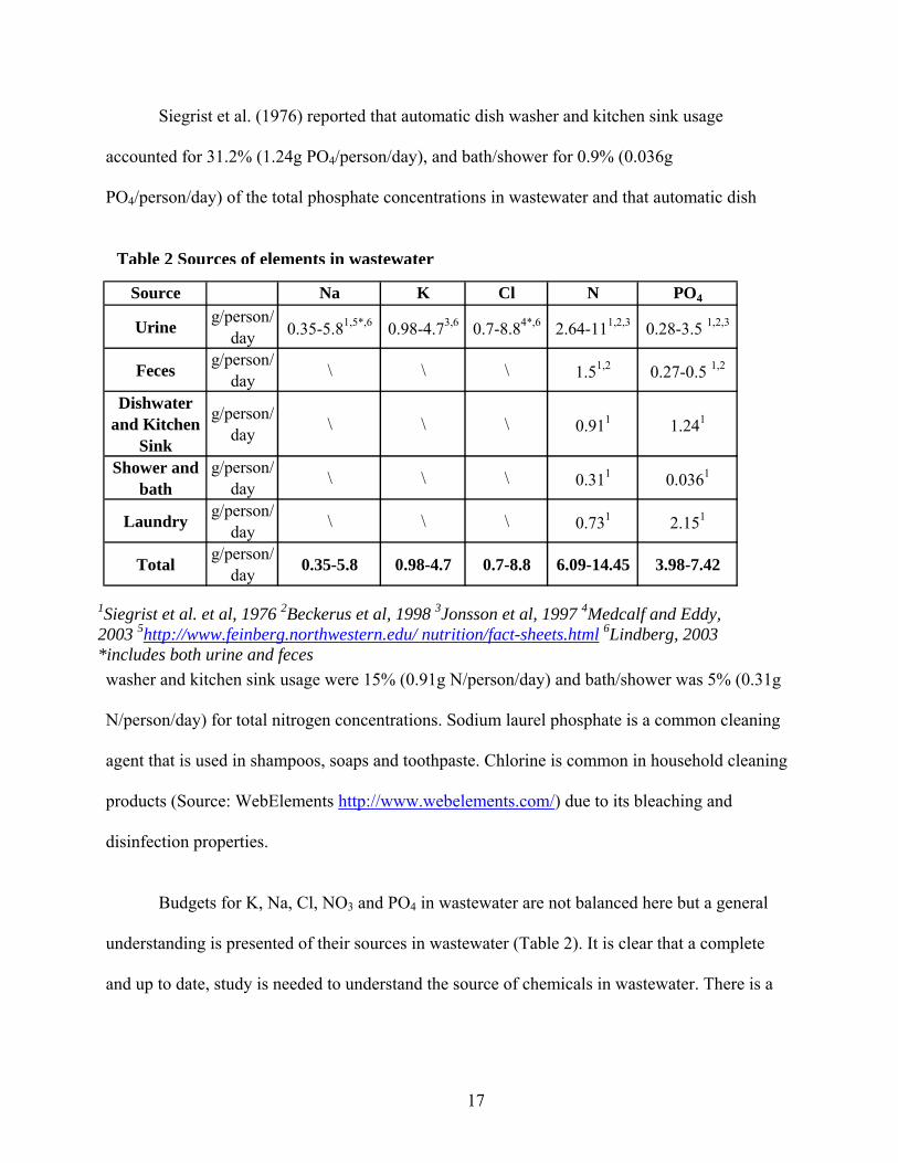
http://www.feinberg.northwestern.edu/ nutrition/fact-sheets.html

Siegrist et al. (1976) reported that automatic dish washer and kitchen sink usage

accounted for 31.2% (1.24g PO4/person/day), and bath/shower for 0.9% (0.036g

PO4/person/day) of the total phosphate concentrations in wastewater and that automatic dish

washer and kitchen sink usage were 15% (0.91g N/person/day) and bath/shower was 5% (0.31g

N/person/day) for total nitrogen concentrations. Sodium laurel phosphate is a common cleaning

agent that is used in shampoos, soaps and toothpaste. Chlorine is common in household cleaning

products (Source: WebElements http://www.webelements.com/) due to its bleaching and

disinfection properties.

Table 2 Sources of elements in wastewater

Source Na K Cl N PO4

Urine g/person/day 0.35-5.81,5*,6 0.98-4.73,6 0.7-8.84*,6 2.64-111,2,3 0.28-3.5 1,2,3

Feces g/person/day \ \ \ 1.51,2 0.27-0.5 1,2

Dishwater and Kitchen

Sink

g/person/day \ \ \ 0.911 1.241

Shower and bath

g/person/day \ \ \ 0.311 0.0361

Laundry g/person/day \ \ \ 0.731 2.151

Total g/person/day 0.35-5.8 0.98-4.7 0.7-8.8 6.09-14.45 3.98-7.42

1Siegrist et al. et al, 1976 2Beckerus et al, 1998 3Jonsson et al, 1997 4Medcalf and Eddy, 2003 5http://www.feinberg.northwestern.edu/ nutrition/fact-sheets.html 6Lindberg, 2003 *includes both urine and feces

Budgets for K, Na, Cl, NO3 and PO4 in wastewater are not balanced here but a general

understanding is presented of their sources in wastewater (Table 2). It is clear that a complete

and up to date, study is needed to understand the source of chemicals in wastewater. There is a

17

http://www.webelements.com/


problem of finding studies that are specific to the United States and since culture influences

eating habits and household products a geographically specific study is important.

Although concentrations of Ca, Mg and SO4 are lower in wastewater than in water

collected below turfgrass sites they are still higher than average groundwater levels. Daily

nutritional requirement are 2500mg Ca and 350 mg Mg (http://www.feinberg.northwestern.edu/

nutrition/fact-sheets.html). Lindberg (2004) reports average values of calcium in urine to be 100-

300mg/person/day. Jonsson et al. (1997) reported in urine concentrations of 18mg Ca/L, 11.1mg

Mg/L and 331mg S/L. Calcium is found in household products such as in toothpastes and used as

a disinfectant and magnesium is present in pharmaceuticals (Source:WebElements

http://www.webelements.com/). Sulfate in wastewater is derived from detergents, disinfectants,

pharmaceutical products and is used in cleaning cesspools (Bleifuss et al., 2000).

18



http://www.webelements.com/

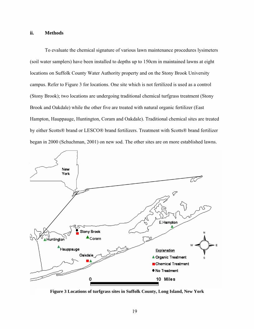
ii. Methods

To evaluate the chemical signature of various lawn maintenance procedures lysimeters

(soil water samplers) have been installed to depths up to 150cm in maintained lawns at eight

locations on Suffolk County Water Authority property and on the Stony Brook University

campus. Refer to Figure 3 for locations. One site which is not fertilized is used as a control

(Stony Brook); two locations are undergoing traditional chemical turfgrass treatment (Stony

Brook and Oakdale) while the other five are treated with natural organic fertilizer (East

Hampton, Hauppauge, Huntington, Coram and Oakdale). Traditional chemical sites are treated

by either Scotts® brand or LESCO® brand fertilizers. Treatment with Scotts® brand fertilizer

began in 2000 (Schuchman, 2001) on new sod. The other sites are on more established lawns.

Treatment using LESCO® brand fertilizer commenced in 2003 with a granular grade fertilizer.

Natural organic treatment, started in spring of 2002, is maintained by Eco-Logical Organic

Landscape, a contract landscaper utilizing athletic turf mix, compost, lime and a granular

fertilizer of either Pro-Grow manufactured by North County Organics or Healthy Turf by Plant

Health Care. Fertilizer regimes are representative of typical applications on Long Island (as

shown in Table 8, Chapter 2). Soil water samples from lysimeters were acquired monthly

totaling 70 samples; 12 samples influenced by traditional chemical fertilizer, 53 influenced by

natural organic fertilizer and 5 influenced by no fertilizer.

Twelve wastewater samples from septic tanks/cesspool systems and 21 public sewage

treatment plant influent samples were acquired through Suffolk County Department of Public

Works. Cesspool samples are from either residential or industrial sources, while a sewage

treatment plant may include residential and industrial sources. Wastewater samples were Figure 3 Locations of turfgrass sites in Suffolk County, Long Island, New York

19

prepared by centrifuging in an International Equipment Corporation (IEC) Model CS floor

mounted centrifuge at 2000 RPM for an hour to separate the solids from the liquid. If necessary

the liquid was decanted and centrifuged again. The liquid was then filtered with Millipore AP15

glass fiber filter.

All samples were collected in polypropylene plastic bottles. Polypropylene plastic bottles

for cation samples were acid rinsed and the samples were preserved with a few drops of HCl.

Samples were stored at 4ºC until analyzed. The samples were analyzed at Cornell University

Nutrient and Elemental Analysis Laboratory. Cation concentrations were determined using an

inductively coupled plasma optical emission spectroscopy (ICP-OES). Anion concentrations

were determined using an ion chromatograph (IC).

The detection limits using IC for Cl, Fl and SO4 are 0.1 ppm, for NO3 and Br 0.2ppm and

for PO4 0.5ppm. The precision and accuracy based on anonymous standards and duplicate

analyses for Cl, F, Br, and SO4 is 10% and for PO4 is 20% and NO3 is 15%. The uncertainty

associated with the precision is high for phosphate due to low phosphate concentrations.

B, Ca, Mg, Na, K, P and S were analyzed on the ICP-OES. The detection limits are for B

0.0005 ppm, Ca 0.002ppm, K 0.13ppm, Mg 0.0001ppm, Na 0.05ppm, P 0.001ppm and S

0.003ppm. The precision and accuracy determined from standards and anonymous duplicate

samples for B, S, Na, and Ca are 10%, for Mg 5%, for K 15% and for phosphorous 20% (high

due to low concentrations).

Average rain water composition was compiled from the literature for Suffolk County

(Proios and Schoonen, 1994; Schoonen and Brown, 1994).

20

iii. Results

One hundred and three samples were analyzed for major and minor ion concentrations,

from which 13 elements were found to be most promising for tracer work (Table 3). These are

NO3, SO4, PO4, B, Ca, Mg, Na, K, Cl, F, Br, P and S. My analysis of nitrate sources in

residential areas show elevated concentrations in Ca, Mg and SO4 in soil water influenced by

turfgrass maintenance compared to wastewater samples. Wastewater samples were enriched in

K, Na, Cl, N-NO3 and PO4 compared to water influenced by turfgrass maintenance.

Concentrations in rain water for major elements are lower than wastewater and soil water

collected below turfgrass sites.

Ca and Mg are enriched in soil water collected below turfgrass plots due to the addition

of lime to maintain a neutral pH and SO4 is from the fertilizers used.

Assuming the average cesspool in Long Island discharges 240 gallons (900 L) per day

(Flynn, 1969), that three people occupy a home, using data from Table 2 and the concentrations

of wastewater found in this study we can calculate contributions of the elements to a cesspool.

Urine and feces would contribute 28% (13.6 ppm) of the nitrogen in wastewaters using raw

concentrations from Siegrist et al. (1976) while data from Beckerus et al. (1998) would suggest

85% (41ppm). Jonsson et al. (1997) only analyzed urine and his study suggests 27% (13 ppm) of

the nitrogen in wastewater comes from urine. Siegrist et al. (1976) study suggest that of the

nitrogen in wastewater 5% (2.4 ppm) comes from clothes washers, 6.5% (3 ppm) comes from

dishwasher and kitchen sink and 2% (1 ppm) comes from showers and baths. Data from Siegrist

et al. (1976) would suggest 13.5% (1.85 ppm) of phosphate in wastewater is from urine and feces

and data from Beckerus et al. (1998) would account for 36% (5 ppm). Data of only urine from

21

Jonsson et al. (1997) suggest 8.5% (1.15ppm) of phosphate in wastewater is from urine. Siegrist

et al. (1976) suggest that of the PO4 in wastewater 52% (7.1 ppm) is from clothes washers, 27%

(4 ppm) comes from the dishwasher and kitchen sink and less than 1% is from showers and

baths. Data from Medcalf and Eddy (2003) suggest Cl in urine and feces account for 41% (19

ppm) of the concentration in wastewaters. Jonsson et at. (1997) analysis of urine would account

for 9% (3.96 ppm) of the Na and 30% (3.3 ppm) of the K in wastewater. Data from Lindberg

(2004) suggest that urine from a typical healthy adult would for <1% (0.06 ppm) Ca, 1% (0.04

ppm) Mg and 19% (1.1 ppm) sulfur in wastewater.

N-NO3 data for wastewater samples in Table 3 were for that of the influent and do not

represent the nitrate concentrations entering the groundwater. Most of the nitrogen produced in a

home is organic nitrogen and urea. Urea breaks down to form ammonia (NH3). Total ammonia is

usually reported as NH3(gas) + NH3(aq) + NH4(aq) (Stumm and Morgan, 1996). In the septic tank

NH3 quickly converts to ammonium, NH4+. Some organic nitrogen in the septic tank also breaks

down to NH4+ but is predominantly present as organic nitrogen (Andreoli et al., 1977). Studies

report around a 20% loss in total nitrogen between the waste that enters a septic tank and when it

enters the cesspool (Porter, 1997; Andreoli et al., 1977). This loss is most likely as ammonia gas.

In the cesspool the BOD (biological oxygen demand) is high and any oxygen present is quickly

consumed. As the effluent travels away from the cesspool the biological oxygen demand

decreases and the conditions become more oxidizing. Dissolved oxygen measurements from

Stackelberg (1995) suggest that soils on Long Island are well drained and well aerated and that

processes that deplete dissolved oxygen, such as nitrification, are insufficient to exhaust

dissolved oxygen supplies. These conditions favor nitrification, the conversion of the various

forms of nitrogen to nitrate by microbial bacteria. N2O can occur as a by-product during

22

nitrification (Stumm and Morgan, 1996) which may also explain small losses in total nitrogen

from the cesspool to the groundwater. Losses here may also be due to soil adsorption of

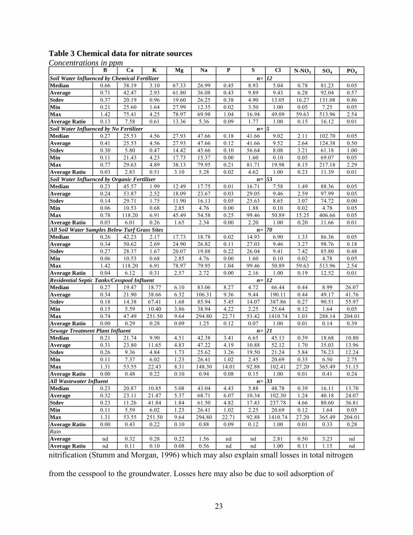
Table 3 Chemical data for nitrate sources Concentrations in ppm

B Ca K Mg Na P S Cl N-NO3 SO4 PO4

Soil Water Influenced by Chemical Fertilizer n= 12Median 0.66 38.19 3.10 67.33 26.99 0.45 8.93 5.04 0.78 81.23 0.05Average 0.71 42.47 2.93 61.80 36.08 0.43 9.89 9.43 6.28 92.04 0.57Stdev 0.37 20.19 0.96 19.60 26.25 0.38 4.90 13.05 16.27 131.08 0.86Min 0.21 25.60 1.64 27.99 12.35 0.02 3.50 1.00 0.05 7.25 0.05Max 1.42 75.41 4.25 78.97 69.98 1.04 16.94 49.09 59.63 513.96 2.54Average Ratio 0.13 7.58 0.61 13.36 5.36 0.09 1.77 1.00 0.15 16.12 0.01Soil Water Influenced by No Fertilizer n= 5Median 0.27 25.53 4.56 27.93 47.66 0.18 41.66 9.02 2.11 102.70 0.05Average 0.41 25.53 4.56 27.93 47.66 0.12 41.66 9.52 2.64 124.38 0.50Stdev 0.30 5.80 0.47 14.42 45.66 0.10 56.64 8.08 3.21 61.18 1.00Min 0.11 21.43 4.23 17.73 15.37 0.00 1.60 0.10 0.05 69.07 0.05Max 0.77 29.63 4.89 38.13 79.95 0.21 81.71 19.98 8.15 217.18 2.29Average Ratio 0.03 2.83 0.51 3.10 5.28 0.02 4.62 1.00 0.23 11.39 0.01Soil Water Influenced by Organic Fertilizer n= 53Median 0.23 45.57 1.99 12.49 17.75 0.01 16.71 7.58 1.49 88.36 0.05Average 0.24 53.87 2.52 18.09 23.67 0.03 29.05 9.46 2.59 97.99 0.05Stdev 0.14 29.71 1.75 11.90 16.13 0.05 25.63 8.65 3.07 74.72 0.00Min 0.06 10.53 0.68 2.85 4.76 0.00 1.88 0.10 0.02 4.78 0.05Max 0.78 118.20 6.91 45.49 54.58 0.25 99.46 50.89 15.25 406.66 0.05Average Ratio 0.03 6.01 0.26 1.65 2.34 0.00 2.20 1.00 0.20 11.66 0.01All Soil Water Samples Below Turf Grass Sites n= 70Median 0.26 42.23 2.17 17.73 18.78 0.02 14.93 6.90 1.33 86.36 0.05Average 0.34 50.62 2.69 24.90 26.82 0.11 27.03 9.46 3.27 98.76 0.18Stdev 0.27 28.37 1.67 20.07 19.88 0.22 26.04 9.41 7.42 85.80 0.48Min 0.06 10.53 0.68 2.85 4.76 0.00 1.60 0.10 0.02 4.78 0.05Max 1.42 118.20 6.91 78.97 79.95 1.04 99.46 50.89 59.63 513.96 2.54Average Ratio 0.04 6.12 0.31 2.57 2.72 0.00 2.16 1.00 0.19 12.52 0.01Residential Septic Tanks/Cesspool Influent n= 12Median 0.27 19.47 18.77 6.10 83.06 8.27 4.72 66.44 0.44 8.99 26.07Average 0.34 21.90 38.66 6.32 106.31 9.36 9.44 190.11 0.44 49.17 41.76Stdev 0.18 14.38 67.41 1.68 85.94 5.45 14.07 387.86 0.27 90.51 55.97Min 0.15 5.59 10.40 3.86 38.94 4.22 2.25 25.64 0.12 1.64 0.05Max 0.74 47.49 251.50 9.64 294.80 22.71 53.42 1410.74 1.03 288.14 204.01Average Ratio 0.00 0.29 0.28 0.09 1.25 0.12 0.07 1.00 0.01 0.14 0.39Sewage Treatment Plant Influent n= 21Median 0.21 21.74 9.90 4.51 42.38 3.41 6.65 45.13 0.39 18.68 10.80Average 0.31 23.80 11.65 4.83 47.22 4.19 10.88 52.12 1.70 35.03 13.96Stdev 0.26 9.36 4.84 1.73 25.62 3.26 19.50 21.24 5.84 76.23 12.24Min 0.11 7.37 6.02 1.23 26.41 1.02 2.45 20.69 0.35 6.50 2.75Max 1.31 53.55 22.43 8.31 148.30 14.01 92.88 102.41 27.20 365.49 51.15Average Ratio 0.00 0.48 0.22 0.10 0.94 0.08 0.15 1.00 0.01 0.41 0.24All Wastewater Influent n= 33Median 0.23 20.87 10.85 5.08 43.04 4.43 5.88 48.78 0.39 16.11 13.70Average 0.32 23.11 21.47 5.37 68.71 6.07 10.34 102.30 1.24 40.18 24.07Stdev 0.23 11.26 41.84 1.84 61.50 4.82 17.43 237.78 4.66 80.60 36.81Min 0.11 5.59 6.02 1.23 26.41 1.02 2.25 20.69 0.12 1.64 0.05Max 1.31 53.55 251.50 9.64 294.80 22.71 92.88 1410.74 27.20 365.49 204.01Average Ratio 0.00 0.43 0.22 0.10 0.88 0.09 0.12 1.00 0.01 0.33 0.28RainAverage nd 0.32 0.28 0.22 1.56 nd nd 2.81 0.50 3.23 ndAverage Ratio nd 0.11 0.10 0.08 0.56 nd nd 1.00 0.11 1.15 nd

23

ammonium that doesn’t convert to nitrate. More studies are needed to understand nitrogen

speciation from the cesspool to the groundwater table. Nitrification occurs before denitrification,

which is the reduction of NO3- to nitrogen gas. For denitrification to occur, the dissolved oxygen

level must be at or near zero. The conditions near the cesspool favor denitrification yet the

nitrogen species is ammonium. It is unlikely that much of the nitrogen is denitrified based on

dissolved oxygen measurements in groundwater samples from Northport (Bleifuss et al., 2000)

and other locations on Long Island (Leamond et al., 1992; Stackelberg, 1995). Porter (1977)

assumed a 50% nitrogen reduction from the raw sewage to the groundwater although he reported

only one study with reductions this high (Andreoli et al., 1977) on Long Island . This study

however is a pilot study which introduced methanol in the leaching field to promote

denitrification. A 50% reduction is thus a high estimate of nitrogen reduction. Porter (1977) does

note that many studies are incomplete and contradictory, thus the need for future work. The

Suffolk County Health Department requirements are for a septic tank attached to a single 12 foot

high stack of , 8’ diameter, pre-cast concrete leaching rings or alternatively, multiple shorter

leaching stacks depending on the depth to groundwater and number of bedrooms (Mermelstein

and Minei, 1995).

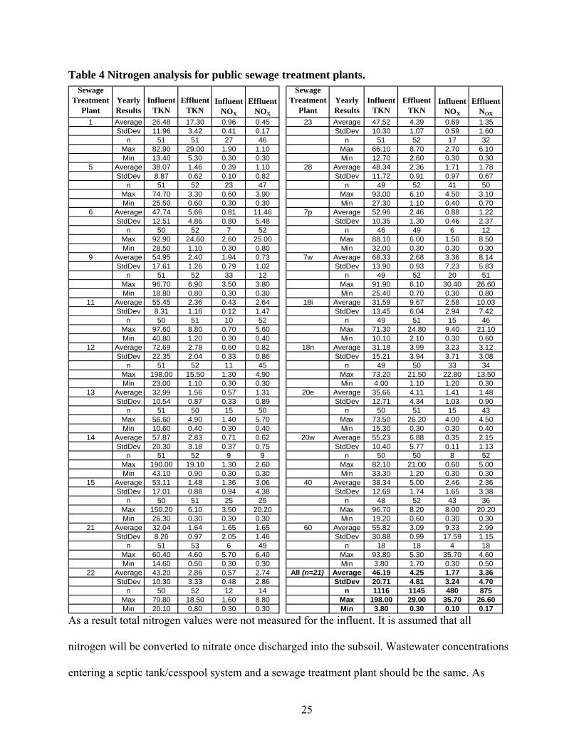
Nitrogen nitrate values for septic tank/cesspool samples were assumed to be the average

sum of all nitrogen species in the influent for the sewage treatment plants for the month of

September, a value of 48 ppm as nitrogen (Table 4). The average for September (48 ppm) and

the year (46 ppm) were not significantly different. The sewage samples analyzed for major

elements were also collected in September. Suffolk County Public Works intended to analyze the

wastewater samples for total nitrogen at the time of collection. However, due to

miscommunication analysis of the samples could not occur before degradation of the samples.

24

As a result total nitrogen values were not measured for the influent. It is assumed that all

nitrogen will be converted to nitrate once discharged into the subsoil. Wastewater concentrations

entering a septic tank/cesspool system and a sewage treatment plant should be the same. As

Table 4 Nitrogen analysis for public sewage treatment plants. Sewage

Treatment Plant

Yearly Results

Influent TKN

Effluent TKN

Influent NOX

Effluent NOX

Sewage Treatment

PlantYearly Results

Influent TKN

Effluent TKN

Influent NOX

Effluent NOX

1 Average 26.48 17.30 0.96 0.45 23 Average 47.52 4.39 0.69 1.35StdDev 11.96 3.42 0.41 0.17 StdDev 10.30 1.07 0.59 1.60

n 51 51 27 46 n 51 52 17 32Max 82.90 29.00 1.90 1.10 Max 66.10 8.70 2.70 6.10Min 13.40 5.30 0.30 0.30 Min 12.70 2.60 0.30 0.30


n 51 52 23 47 n 49 52 41 50Max 74.70 3.30 0.60 3.90 Max 93.00 6.10 4.50 3.10Min 25.50 0.60 0.30 0.30 Min 27.30 1.10 0.40 0.70

6 Average 47.74 5.66 0.81 11.46 7p Average 52.96 2.46 0.88 1.22StdDev 12.51 4.86 0.80 5.48 StdDev 10.35 1.30 0.46 2.37

n 50 52 7 52 n 46 49 6 12Max 92.90 24.60 2.60 25.00 Max 88.10 6.00 1.50 8.50Min 28.50 1.10 0.30 0.80 Min 32.00 0.30 0.30 0.30

9 Average 54.95 2.40 1.94 0.73 7w Average 68.33 2.68 3.36 8.14StdDev 17.61 1.26 0.79 1.02 StdDev 13.90 0.93 7.23 5.83

n 51 52 33 12 n 49 52 20 51Max 96.70 6.90 3.50 3.80 Max 91.90 6.10 30.40 26.60Min 18.80 0.80 0.30 0.30 Min 25.40 0.70 0.30 0.80

11 Average 55.45 2.36 0.43 2.64 18i Average 31.59 9.67 2.58 10.03StdDev 8.31 1.16 0.12 1.47 StdDev 13.45 6.04 2.94 7.42

n 50 51 10 52 n 49 51 15 46Max 97.60 8.80 0.70 5.60 Max 71.30 24.80 9.40 21.10Min 40.80 1.20 0.30 0.40 Min 10.10 2.10 0.30 0.60

12 Average 72.69 2.78 0.60 0.82 18n Average 31.18 3.99 3.23 3.12StdDev 22.35 2.04 0.33 0.86 StdDev 15.21 3.94 3.71 3.08

n 51 52 11 45 n 49 50 33 34Max 198.00 15.50 1.30 4.90 Max 73.20 21.50 22.80 13.50Min 23.00 1.10 0.30 0.30 Min 4.00 1.10 1.20 0.30

13 Average 32.99 1.56 0.57 1.31 20e Average 35.66 4.11 1.41 1.48StdDev 10.54 0.87 0.33 0.89 StdDev 12.71 4.34 1.03 0.90

n 51 50 15 50 n 50 51 15 43Max 56.60 4.90 1.40 5.70 Max 73.50 26.20 4.00 4.50Min 10.60 0.40 0.30 0.40 Min 15.30 0.30 0.30 0.40

14 Average 57.87 2.83 0.71 0.62 20w Average 55.23 6.88 0.35 2.15StdDev 20.30 3.18 0.37 0.75 StdDev 10.40 5.77 0.11 1.13

n 51 52 9 9 n 50 50 8 52Max 190.00 19.10 1.30 2.60 Max 82.10 21.00 0.60 5.00Min 43.10 0.90 0.30 0.30 Min 33.30 1.20 0.30 0.30


n 50 51 25 25 n 48 52 43 36Max 150.20 6.10 3.50 20.20 Max 96.70 8.20 8.00 20.20Min 26.30 0.30 0.30 0.30 Min 19.20 0.60 0.30 0.30


n 51 53 6 49 n 18 18 4 18Max 60.40 4.60 5.70 6.40 Max 93.80 5.30 35.70 4.60Min 14.60 0.50 0.30 0.30 Min 3.80 1.70 0.30 0.50

22 Average 43.20 2.86 0.57 2.74 All (n=21) Average 46.19 4.25 1.77 3.36StdDev 10.30 3.33 0.48 2.86 StdDev 20.71 4.81 3.24 4.70

n 50 52 12 14 n 1116 1145 480 875Max 79.80 18.50 1.60 8.80 Max 198.00 29.00 35.70 26.60Min 20.10 0.80 0.30 0.30 Min 3.80 0.30 0.10 0.17

25

evident in Table 4, the sewage treatment plants in this study reduce nitrogen concentrations to

below the drinking water standard and usually below 5 ppm before discharge. Therefore the

effluent for a sewage treatment plant has much lower concentrations of nitrogen than a septic

tank/cesspool system and yield similar ratios of the elements to chloride as rainwater in the

source plots. It was therefore decided not include them as a source field in the data plots since

their influence of nitrate concentrations in groundwater is likely to be minimal.

Geochemical tracer source plots

A combination of the elements N-NO3, SO4, Na, Ca, Mg and Cl plotted on binary plots

and a ternary diagram can place constraints of nitrate sources for a given groundwater. The most

useful groundwater geochemical tracer is a conservative element, which is one that does not

adsorb to the soil surfaces, or degrade with time due to biological or physical processes. N-NO3,

Cl and SO4 are the most conservative elements utilized here. The cations Ca, Mg and Na tend to

adsorb to negatively charged soil particles but with accurate sorption modeling such as done by

Voegelin et al. (2000) and an understanding of plant uptake, concentrations in groundwater may

be predicted.

Density contours were created for the two source fields 1) soil water collected below

turfgrass sites treated with traditional chemical fertilizer, natural organic fertilizer or no fertilizer

(gray scale) and 2) wastewater from septic tank/cesspool systems (color scale). Although there is

a statistical difference in the concentrations of the soil waters their fields overlapped and

therefore all soil water data is plotted as one field. Since the public sewage treatment plants

analyzed in this study reduce nitrate concentrations before discharge they are contributing fewer

nitrates to the groundwater and are not plotted as a source on the plots. They are however a

26

source of groundwater recharge when the discharge location for the sewage treatment plant is

within the capture zone for a given groundwater well.

Density contours for binary plots were created using the Fortran 77 programming

language and Absoft compiler (complied by Professor Daniel Davis, SUNY Stony Brook, 2003).

For this method the X and Y data ranges were divided into 151 segment each, for a total of

22,801 bins for each plot. A Gaussian (normal) bivariate distribution is calculated for each data

point, distributing that data point among bins with an assumption that the standard deviation in

each axis equals 10% of the measured value in that axis. A normal distribution for a data point X

with mean (µ) and standard deviation (σ) is a statistical distribution with a probability function

)2()(

2

2

21)( σ

µ

πσ

−−

=x

exP eq. 1

(Mathworld, WOLFRAM Research, http://mathworld.wolfram.com ). Eq. 1 is applied in both the

X and Y directions. For values approaching zero, a minimum standard deviation is defined, equal

to 0.05 in X and Y. A Gaussian distribution (defined as a bell shaped curve) is defined out to 3

sigma in both the X and Y directions, such that the integral over the curve equals one (except

when part of the curve falls in the range of impossible negative values). The contribution to a

given bin from a given point corresponds to the probability that that value actually falls with in

the X-Y range defined by that bin. The contribution from each data point is summed for each of

the bins, producing a data density plot that represents the best available estimate of the likely

distribution for the variables.

Twenty two Suffolk County Water Authority public supply wells and eight monitoring

wells from Bleifuss et al. (2000) were chosen to represent a range of land use and locations in

27

http://mathworld.wolfram.com/

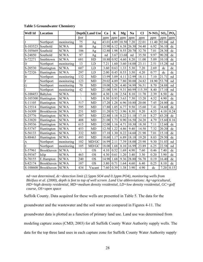
Suffolk County. Data acquired for these wells are presented in Table 5. The data for the

groundwater and the wastewater and the soil water are compared in Figures 4-11. The

groundwater data is plotted as a function of primary land use. Land use was determined from

modeling capture zones (CMD, 2003) for all Suffolk County Water Authority supply wells. The

data for the top three land uses in each capture zone for Suffolk County Water Authority supply

Well Id Location Depth Land Use Ca K Mg Na Cl N-NO3 SO4 PO4

feet ppm ppm ppm ppm ppm ppm ppm ppmJ Northport monitoring 75 Ag 43.01 4.89 10.50 7.20 22.01 11.40 92.04 ndS-103523 Southold SCWA 88 Ag 15.90 6.12 6.38 26.30 54.40 6.92 36.10 dcS-105669 Southold SCWA 106 Ag 12.80 1.98 8.55 20.70 32.70 7.01 28.30 dcS-24850 Southold SCWA 97 Ag nd 3.67 13.68 nd 35.50 9.97 90.20 dcS-72271 Smithtown SCWA 681 HD 10.80 0.92 4.60 8.20 11.00 5.09 10.10 dcD Northport monitoring 13 LD 7.21 1.60 3.60 14.00 23.11 2.51 15.28 ndS-20530 Huntington SCWA 607 LD 3.60 0.63 1.33 5.30 7.20 2.69 dc dcS-72326 Huntington SCWA 297 LD 2.00 0.45 0.53 3.50 4.20 0.77 dc dcB Northport monitoring 132 MD 13.99 3.09 4.11 12.99 18.11 7.10 21.71 ndF Northport monitoring 123 MD 29.02 4.89 7.80 30.00 24.82 18.90 53.70 ndG Northport monitoring 70 MD 19.00 3.28 4.40 34.99 56.51 8.70 24.88 ndI Northport monitoring 42 MD 21.00 3.91 9.31 60.99 115.39 8.40 17.10 ndS-100453 Babylon SCWA \ MD 4.30 1.18 2.54 8.10 11.70 2.39 8.50 dcS-105300 Huntington SCWA \ MD 8.30 0.93 3.63 7.30 13.20 4.52 4.90 dcS-11105 Huntington SCWA 517 MD 17.20 1.28 6.96 10.80 20.00 7.45 24.00 dcS-15514 Huntington SCWA 595 MD 17.80 1.05 6.77 9.50 15.60 7.41 34.60 dcS-16309 Brookhaven SCWA 251 MD 11.20 0.72 3.96 8.30 9.20 4.55 4.10 0.24S-25776 Huntington SCWA 587 MD 22.80 1.18 8.22 11.10 17.10 8.27 43.20 dcS-33820 Huntington SCWA 408 MD 21.00 1.73 8.90 16.50 24.20 4.79 15.60 0.16S-39536 Huntington SCWA 615 MD 12.00 1.16 4.71 10.30 18.30 7.11 12.60 dcS-53747 Huntington SCWA 453 MD 12.50 1.22 4.86 9.40 14.50 7.32 20.20 dcS-56133 Huntington SCWA 332 MD 17.10 1.30 8.22 14.60 21.90 7.01 15.10 dcS-88463 Huntington SCWA 493 MD 18.60 1.17 6.89 18.10 19.20 8.03 29.50 dcA Northport monitoring 102 MD/GC 16.99 2.11 7.39 18.00 25.98 9.30 31.03 ndE Northport monitoring 105 MD/GC 18.00 1.68 8.10 16.99 23.89 6.25 22.58 ndS-57961 Brookhaven SCWA \ OS 4.10 0.52 1.69 4.90 7.60 0.46 7.40 dcS-59347 Islip SCWA 463 OS 4.30 0.61 1.20 3.40 3.30 0.20 3.90 dcS-70155 E.Hampton SCWA 240 OS 14.90 1.68 9.36 28.80 56.70 0.19 16.40 dcS-82174 Brookhaven SCWA 187 OS 3.80 0.71 1.64 4.60 6.40 0.25 8.10 dcS-100608 Brookhaven SCWA 434 Vacant 7.60 0.39 1.38 3.90 4.90 dc 7.20 0.15

nd=not determined, dc=detection limit (2.5ppm SO4 and 0.1ppm PO4), monitoring wells from Bleifuss et al. (2000), depth is feet to top of well screen .Land Use abbreviations: Ag=agricultural, HD=high density residential, MD=medium density residential, LD=low density residential, GC=golf course, OS=open space

Table 5 Groundwater Chemistry

28

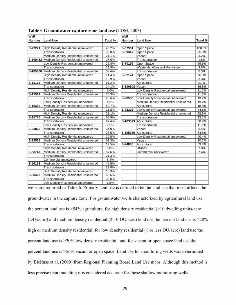
wells are reported in Table 6. Primary land use is defined to be the land use that most affects the

groundwater in the capture zone. For groundwater wells characterized by agricultural land use

the percent land use is >54% agriculture, for high density residential (>10 dwelling units/acre

(DU/acre)) and medium density residential (2-10 DU/acre) land use the percent land use is >28%

high or medium density residential, for low density residential (1 or less DU/acre) land use the

percent land use is >20% low density residential and for vacant or open space land use the

percent land use is >56% vacant or open space. Land use for monitoring wells was determined

by Bleifuss et al. (2000) from Regional Planning Board Land Use maps. Although this method is

less precise than modeling it is considered accurate for these shallow monitoring wells.

Well Number Land Use Total %

Well Number Land Use Total %

S-72271 High Density Residential unsewered 40.2% S-57961 Open Space 100.0%Transportation 30.0% S-59347 Open Space 95.0%Medium Density Residential unsewered 21.1% Vacant 3.2%

S-100453 Medium Density Residential unsewered 28.6% Transportation 1.8%Low Density Residential unsewered 25.8% S-70155 Open Space 89.9%Transportation 19.9% Waste Handling and Maintance 3.8%

S-105300 Medium Density Residential unsewered 59.4% Transportation 3.3%High Density Residential unsewered 14.4% S-82174 Open Space 96.0%Transportation 10.9% Vacant 3.3%

S-11105 Medium Density Residential unsewered 61.2% Agricultural 0.7%Transportation 24.1% S-100608 Vacant 56.5%High Density Residential unsewered 9.0% Low Density Residential unsewered 21.2%

S-15514 Medium Density Residential unsewered 70.3% Transportation 11.8%Transportation 25.6% S-20530 Low Density Residential unsewered 19.4%Low Density Residential unsewered 1.6% Medium Density Residential unsewered 19.2%

S-16309 Medium Density Residential unsewered 50.7% Agricultural 18.8%Transportation 21.8% S-72326 Low Density Residential unsewered 54.8%High Density Residential unsewered 21.1% Medium Density Residential unsewered 28.8%

S-25776 Medium Density Residential unsewered 67.9% Transportation 13.1%Transportation 27.4% S-103523 Agricultural 58.9%Low Density Residential unsewered 2.5% Transportation 11.1%

S-33820 Medium Density Residential unsewered 34.0% Vacant 9.4%Transportation 23.5% S-105669 Agricultural 54.8%High Density Residential unsewered 22.5% Low Density Residential unsewered 20.4%

S-39536 Medium Density Residential unsewered 62.3% Vacant 10.7%Transportation 19.5% S-24850 Agricultural 69.3%High Density Residential unsewered 6.8% Utilities 7.8%

S-53747 Medium Density Residential unsewered 57.6% Commercial unsewered 7.4%Transportation 21.3%Commercial unsewered 5.4%

S-56133 Medium Density Residential unsewered 49.5%Transportation 22.8%High Density Residential unsewered 16.3%

S-88463 Medium Density Residential unsewered 63.6%Transportation 33.0%Low Density Residential unsewered 1.5%

Table 6 Groundwater capture zone land use (CDM, 2003)

29

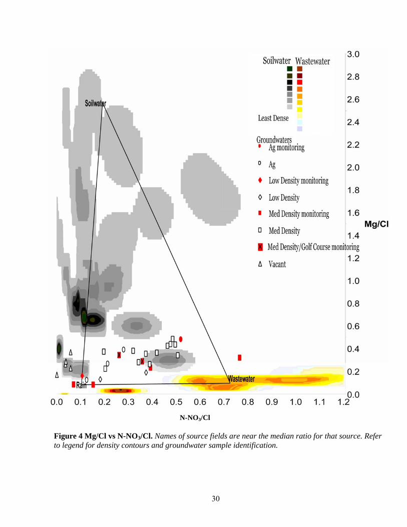
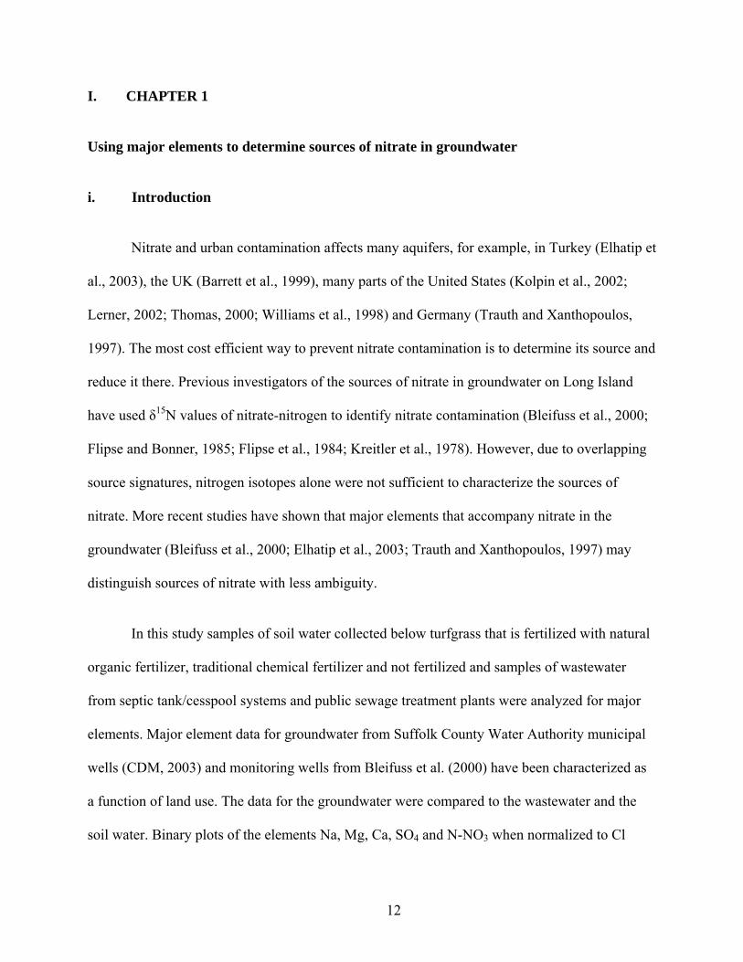
N-NO3/Cl

Figure 4 Mg/Cl vs N-NO3/Cl. Names of source fields are near the median ratio for that source. Refer to legend for density contours and groundwater sample identification.

30

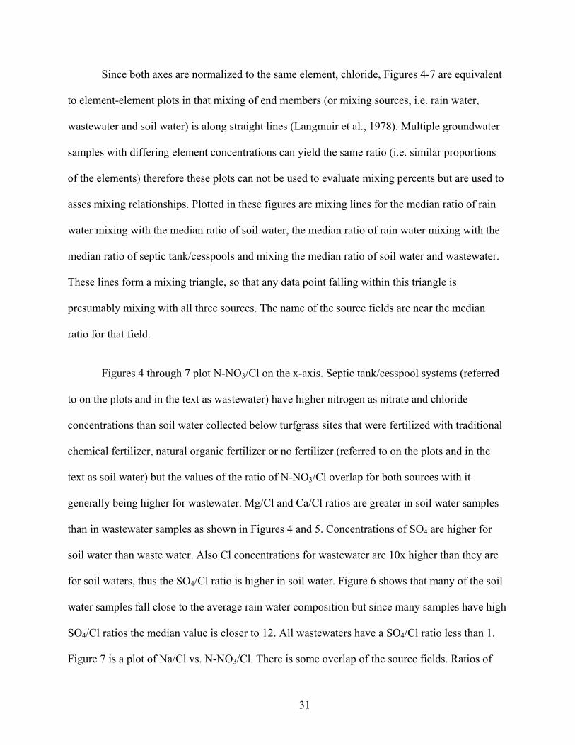
Since both axes are normalized to the same element, chloride, Figures 4-7 are equivalent

to element-element plots in that mixing of end members (or mixing sources, i.e. rain water,

wastewater and soil water) is along straight lines (Langmuir et al., 1978). Multiple groundwater

samples with differing element concentrations can yield the same ratio (i.e. similar proportions

of the elements) therefore these plots can not be used to evaluate mixing percents but are used to

asses mixing relationships. Plotted in these figures are mixing lines for the median ratio of rain

water mixing with the median ratio of soil water, the median ratio of rain water mixing with the

median ratio of septic tank/cesspools and mixing the median ratio of soil water and wastewater.

These lines form a mixing triangle, so that any data point falling within this triangle is

presumably mixing with all three sources. The name of the source fields are near the median

ratio for that field.

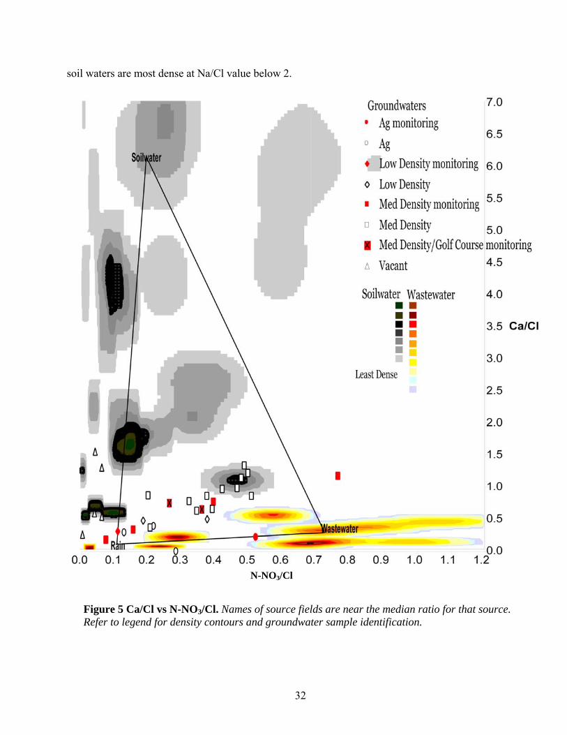
Figures 4 through 7 plot N-NO3/Cl on the x-axis. Septic tank/cesspool systems (referred

to on the plots and in the text as wastewater) have higher nitrogen as nitrate and chloride

concentrations than soil water collected below turfgrass sites that were fertilized with traditional

chemical fertilizer, natural organic fertilizer or no fertilizer (referred to on the plots and in the

text as soil water) but the values of the ratio of N-NO3/Cl overlap for both sources with it

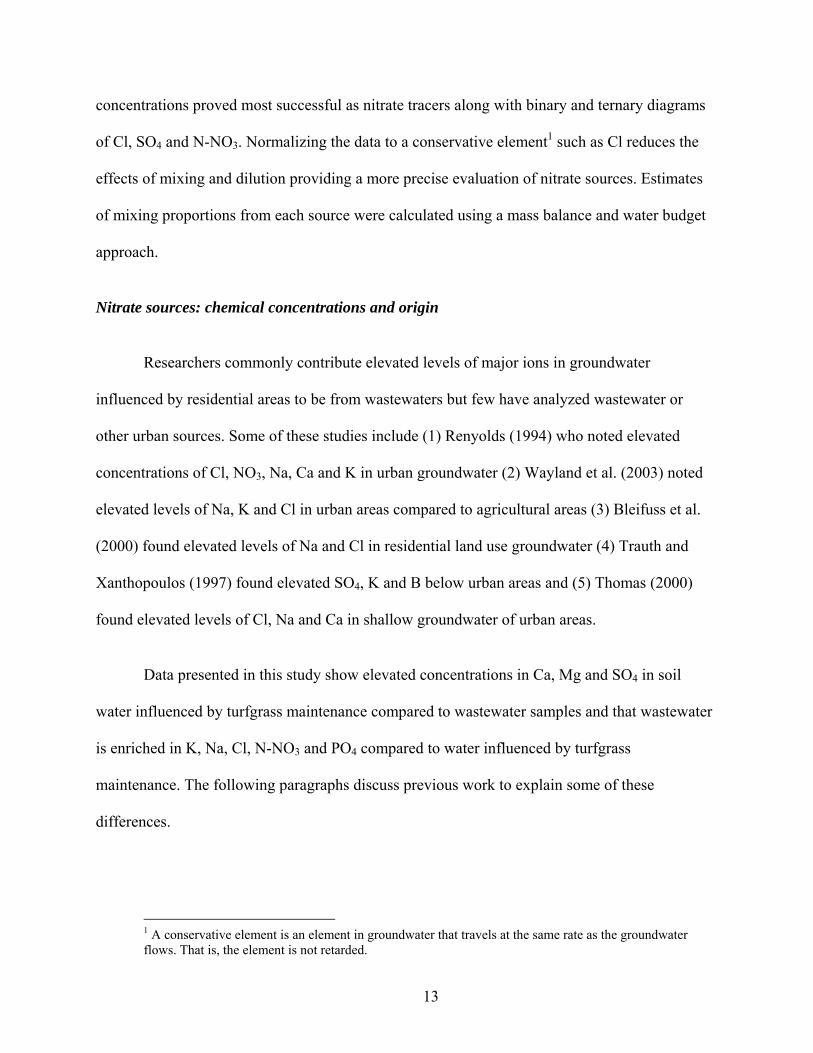
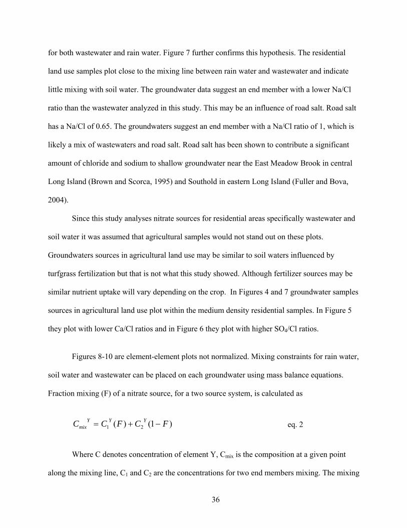
generally being higher for wastewater. Mg/Cl and Ca/Cl ratios are greater in soil water samples

than in wastewater samples as shown in Figures 4 and 5. Concentrations of SO4 are higher for

soil water than waste water. Also Cl concentrations for wastewater are 10x higher than they are

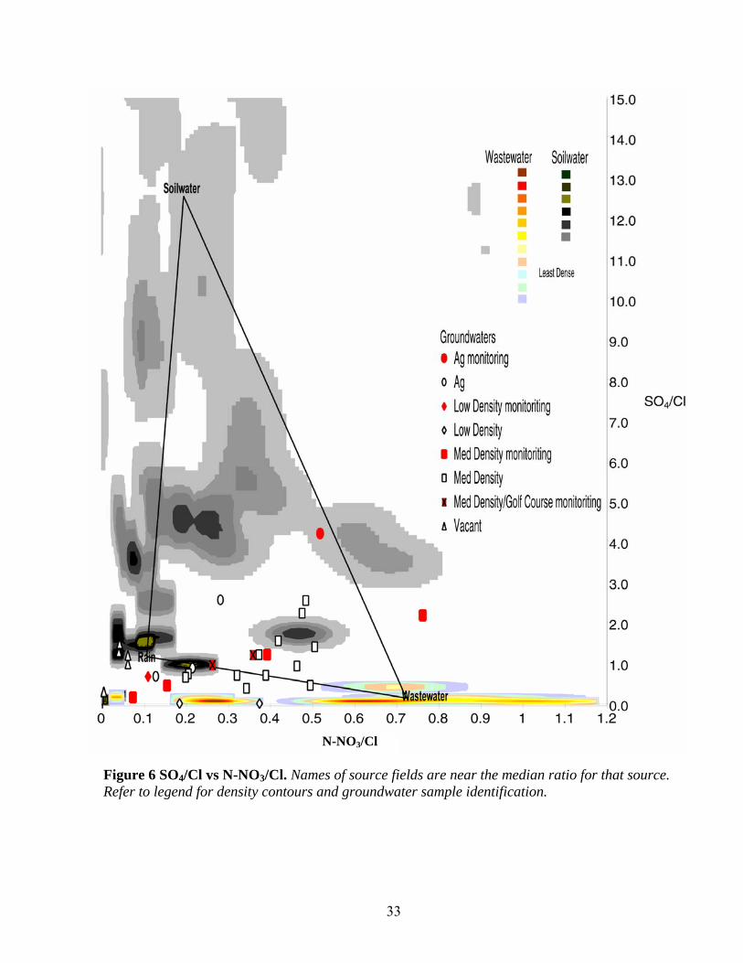
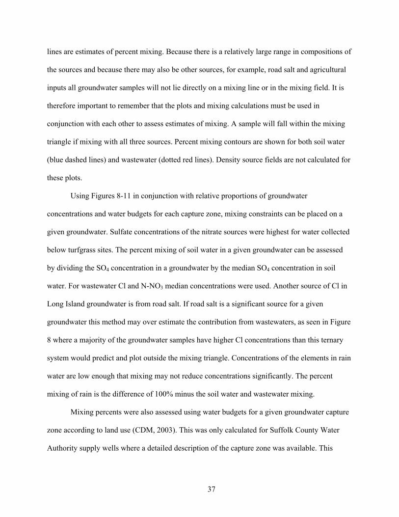
for soil waters, thus the SO4/Cl ratio is higher in soil water. Figure 6 shows that many of the soil

water samples fall close to the average rain water composition but since many samples have high

SO4/Cl ratios the median value is closer to 12. All wastewaters have a SO4/Cl ratio less than 1.

Figure 7 is a plot of Na/Cl vs. N-NO3/Cl. There is some overlap of the source fields. Ratios of

31

soil waters are most dense at Na/Cl value below 2.

N-NO3/Cl

Figure 5 Ca/Cl vs N-NO3/Cl. Names of source fields are near the median ratio for that source. Refer to legend for density contours and groundwater sample identification.

32

33

N-NO3/Cl

Figure 6 SO4/Cl vs N-NO3/Cl. Names of source fields are near the median ratio for that source. Refer to legend for density contours and groundwater sample identification.

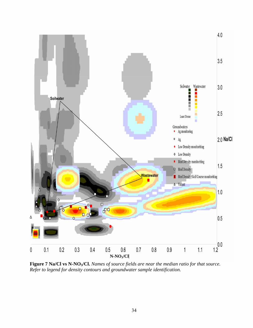
Figure 7 Na/Cl vs N-NO3/Cl. Names of source fields are near the median ratio for that source. Refer to legend for density contours and groundwater sample identification.

N-NO3/Cl

34

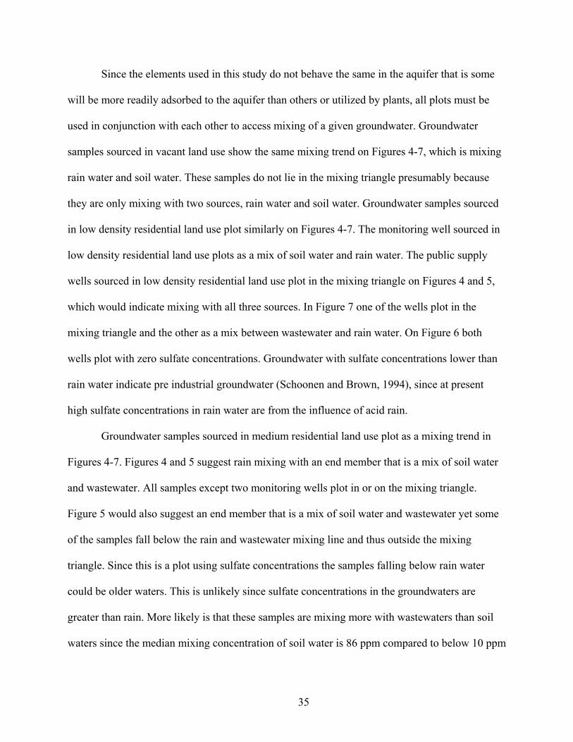
Since the elements used in this study do not behave the same in the aquifer that is some

will be more readily adsorbed to the aquifer than others or utilized by plants, all plots must be

used in conjunction with each other to access mixing of a given groundwater. Groundwater

samples sourced in vacant land use show the same mixing trend on Figures 4-7, which is mixing

rain water and soil water. These samples do not lie in the mixing triangle presumably because

they are only mixing with two sources, rain water and soil water. Groundwater samples sourced

in low density residential land use plot similarly on Figures 4-7. The monitoring well sourced in

low density residential land use plots as a mix of soil water and rain water. The public supply

wells sourced in low density residential land use plot in the mixing triangle on Figures 4 and 5,

which would indicate mixing with all three sources. In Figure 7 one of the wells plot in the

mixing triangle and the other as a mix between wastewater and rain water. On Figure 6 both

wells plot with zero sulfate concentrations. Groundwater with sulfate concentrations lower than

rain water indicate pre industrial groundwater (Schoonen and Brown, 1994), since at present

high sulfate concentrations in rain water are from the influence of acid rain.

Groundwater samples sourced in medium residential land use plot as a mixing trend in

Figures 4-7. Figures 4 and 5 suggest rain mixing with an end member that is a mix of soil water

and wastewater. All samples except two monitoring wells plot in or on the mixing triangle.

Figure 5 would also suggest an end member that is a mix of soil water and wastewater yet some

of the samples fall below the rain and wastewater mixing line and thus outside the mixing

triangle. Since this is a plot using sulfate concentrations the samples falling below rain water

could be older waters. This is unlikely since sulfate concentrations in the groundwaters are

greater than rain. More likely is that these samples are mixing more with wastewaters than soil

waters since the median mixing concentration of soil water is 86 ppm compared to below 10 ppm

35

for both wastewater and rain water. Figure 7 further confirms this hypothesis. The residential

land use samples plot close to the mixing line between rain water and wastewater and indicate

little mixing with soil water. The groundwater data suggest an end member with a lower Na/Cl

ratio than the wastewater analyzed in this study. This may be an influence of road salt. Road salt

has a Na/Cl of 0.65. The groundwaters suggest an end member with a Na/Cl ratio of 1, which is

likely a mix of wastewaters and road salt. Road salt has been shown to contribute a significant

amount of chloride and sodium to shallow groundwater near the East Meadow Brook in central

Long Island (Brown and Scorca, 1995) and Southold in eastern Long Island (Fuller and Bova,

2004).

Since this study analyses nitrate sources for residential areas specifically wastewater and

soil water it was assumed that agricultural samples would not stand out on these plots.

Groundwaters sources in agricultural land use may be similar to soil waters influenced by

turfgrass fertilization but that is not what this study showed. Although fertilizer sources may be

similar nutrient uptake will vary depending on the crop. In Figures 4 and 7 groundwater samples

sources in agricultural land use plot within the medium density residential samples. In Figure 5

they plot with lower Ca/Cl ratios and in Figure 6 they plot with higher SO4/Cl ratios.

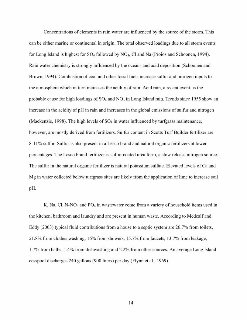
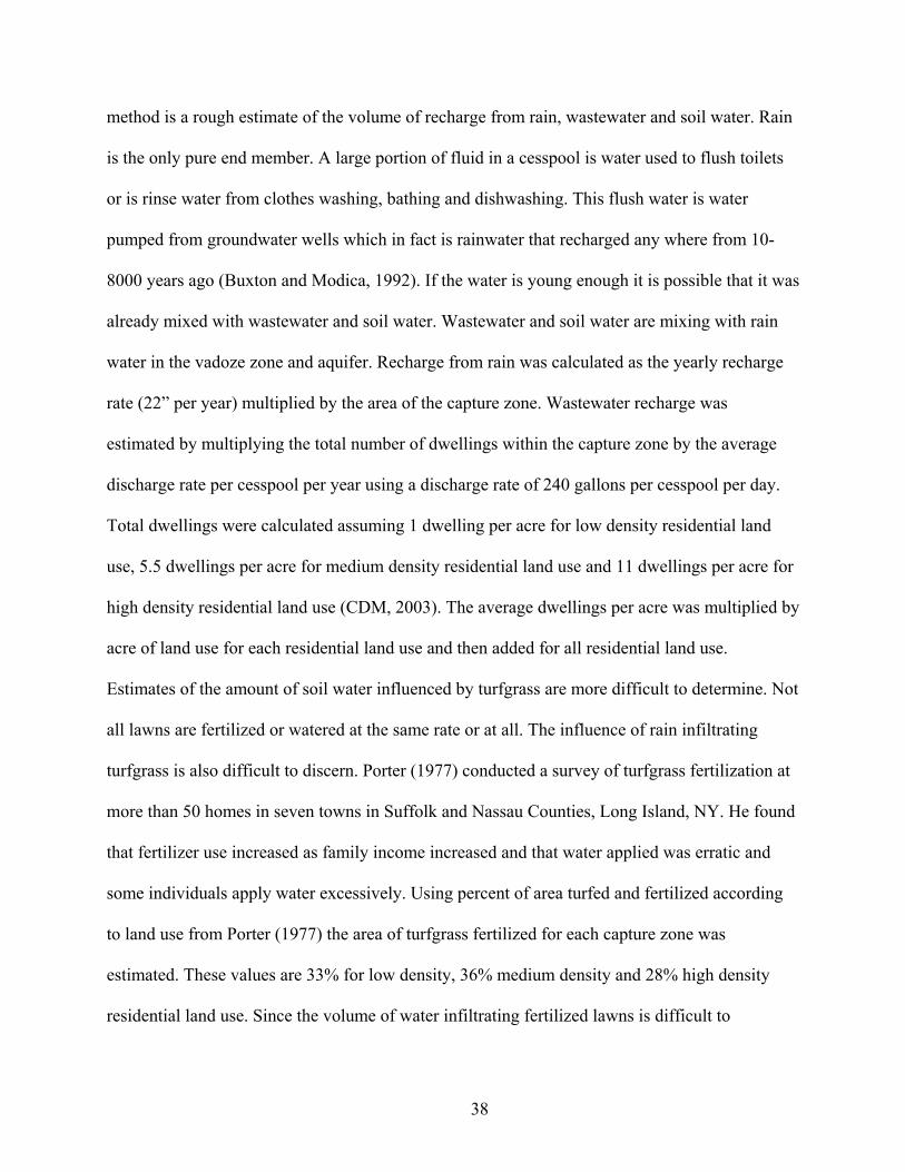
Figures 8-10 are element-element plots not normalized. Mixing constraints for rain water,

soil water and wastewater can be placed on each groundwater using mass balance equations.

Fraction mixing (F) of a nitrate source, for a two source system, is calculated as

eq. 2 )1()( 21 FCFCC YYYmix −+=

Where C denotes concentration of element Y, Cmix is the composition at a given point

along the mixing line, C1 and C2 are the concentrations for two end members mixing. The mixing

36

lines are estimates of percent mixing. Because there is a relatively large range in compositions of

the sources and because there may also be other sources, for example, road salt and agricultural

inputs all groundwater samples will not lie directly on a mixing line or in the mixing field. It is

therefore important to remember that the plots and mixing calculations must be used in

conjunction with each other to assess estimates of mixing. A sample will fall within the mixing

triangle if mixing with all three sources. Percent mixing contours are shown for both soil water

(blue dashed lines) and wastewater (dotted red lines). Density source fields are not calculated for

these plots.

Using Figures 8-11 in conjunction with relative proportions of groundwater

concentrations and water budgets for each capture zone, mixing constraints can be placed on a

given groundwater. Sulfate concentrations of the nitrate sources were highest for water collected

below turfgrass sites. The percent mixing of soil water in a given groundwater can be assessed

by dividing the SO4 concentration in a groundwater by the median SO4 concentration in soil

water. For wastewater Cl and N-NO3 median concentrations were used. Another source of Cl in

Long Island groundwater is from road salt. If road salt is a significant source for a given

groundwater this method may over estimate the contribution from wastewaters, as seen in Figure

8 where a majority of the groundwater samples have higher Cl concentrations than this ternary

system would predict and plot outside the mixing triangle. Concentrations of the elements in rain

water are low enough that mixing may not reduce concentrations significantly. The percent

mixing of rain is the difference of 100% minus the soil water and wastewater mixing.

Mixing percents were also assessed using water budgets for a given groundwater capture

zone according to land use (CDM, 2003). This was only calculated for Suffolk County Water

Authority supply wells where a detailed description of the capture zone was available. This

37

method is a rough estimate of the volume of recharge from rain, wastewater and soil water. Rain

is the only pure end member. A large portion of fluid in a cesspool is water used to flush toilets

or is rinse water from clothes washing, bathing and dishwashing. This flush water is water

pumped from groundwater wells which in fact is rainwater that recharged any where from 10-

8000 years ago (Buxton and Modica, 1992). If the water is young enough it is possible that it was

already mixed with wastewater and soil water. Wastewater and soil water are mixing with rain

water in the vadoze zone and aquifer. Recharge from rain was calculated as the yearly recharge

rate (22” per year) multiplied by the area of the capture zone. Wastewater recharge was

estimated by multiplying the total number of dwellings within the capture zone by the average

discharge rate per cesspool per year using a discharge rate of 240 gallons per cesspool per day.

Total dwellings were calculated assuming 1 dwelling per acre for low density residential land

use, 5.5 dwellings per acre for medium density residential land use and 11 dwellings per acre for

high density residential land use (CDM, 2003). The average dwellings per acre was multiplied by

acre of land use for each residential land use and then added for all residential land use.

Estimates of the amount of soil water influenced by turfgrass are more difficult to determine. Not

all lawns are fertilized or watered at the same rate or at all. The influence of rain infiltrating

turfgrass is also difficult to discern. Porter (1977) conducted a survey of turfgrass fertilization at

more than 50 homes in seven towns in Suffolk and Nassau Counties, Long Island, NY. He found

that fertilizer use increased as family income increased and that water applied was erratic and

some individuals apply water excessively. Using percent of area turfed and fertilized according

to land use from Porter (1977) the area of turfgrass fertilized for each capture zone was

estimated. These values are 33% for low density, 36% medium density and 28% high density

residential land use. Since the volume of water infiltrating fertilized lawns is difficult to

38

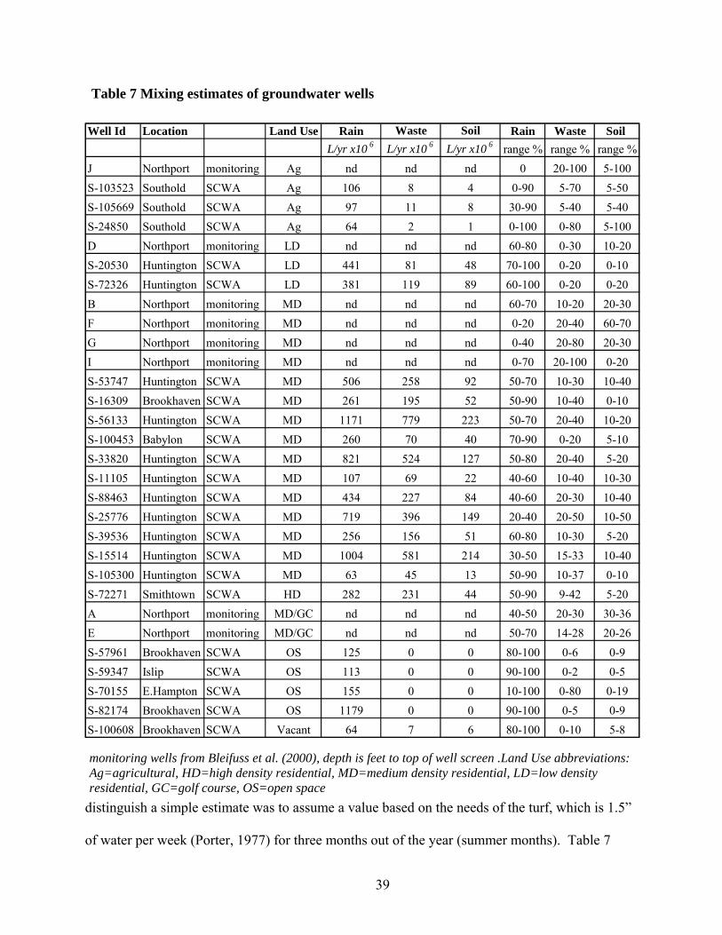
Table 7 Mixing estimates of groundwater wells

Well Id Location Land Use Rain Waste Soil Rain Waste Soil L/yr x10 6 L/yr x10 6 L/yr x10 6 range % range % range %

J Northport monitoring Ag nd nd nd 0 20-100 5-100S-103523 Southold SCWA Ag 106 8 4 0-90 5-70 5-50S-105669 Southold SCWA Ag 97 11 8 30-90 5-40 5-40S-24850 Southold SCWA Ag 64 2 1 0-100 0-80 5-100D Northport monitoring LD nd nd nd 60-80 0-30 10-20S-20530 Huntington SCWA LD 441 81 48 70-100 0-20 0-10S-72326 Huntington SCWA LD 381 119 89 60-100 0-20 0-20B Northport monitoring MD nd nd nd 60-70 10-20 20-30F Northport monitoring MD nd nd nd 0-20 20-40 60-70G Northport monitoring MD nd nd nd 0-40 20-80 20-30I Northport monitoring MD nd nd nd 0-70 20-100 0-20S-53747 Huntington SCWA MD 506 258 92 50-70 10-30 10-40S-16309 Brookhaven SCWA MD 261 195 52 50-90 10-40 0-10S-56133 Huntington SCWA MD 1171 779 223 50-70 20-40 10-20S-100453 Babylon SCWA MD 260 70 40 70-90 0-20 5-10S-33820 Huntington SCWA MD 821 524 127 50-80 20-40 5-20S-11105 Huntington SCWA MD 107 69 22 40-60 10-40 10-30S-88463 Huntington SCWA MD 434 227 84 40-60 20-30 10-40S-25776 Huntington SCWA MD 719 396 149 20-40 20-50 10-50S-39536 Huntington SCWA MD 256 156 51 60-80 10-30 5-20S-15514 Huntington SCWA MD 1004 581 214 30-50 15-33 10-40S-105300 Huntington SCWA MD 63 45 13 50-90 10-37 0-10S-72271 Smithtown SCWA HD 282 231 44 50-90 9-42 5-20A Northport monitoring MD/GC nd nd nd 40-50 20-30 30-36E Northport monitoring MD/GC nd nd nd 50-70 14-28 20-26S-57961 Brookhaven SCWA OS 125 0 0 80-100 0-6 0-9S-59347 Islip SCWA OS 113 0 0 90-100 0-2 0-5S-70155 E.Hampton SCWA OS 155 0 0 10-100 0-80 0-19S-82174 Brookhaven SCWA OS 1179 0 0 90-100 0-5 0-9S-100608 Brookhaven SCWA Vacant 64 7 6 80-100 0-10 5-8

distinguish a simple estimate was to assume a value based on the needs of the turf, which is 1.5”

of water per week (Porter, 1977) for three months out of the year (summer months). Table 7

monitoring wells from Bleifuss et al. (2000), depth is feet to top of well screen .Land Use abbreviations: Ag=agricultural, HD=high density residential, MD=medium density residential, LD=low density residential, GC=golf course, OS=open space

39

reports the water budget and estimated percent contribution for all three nitrate sources, as

described above.

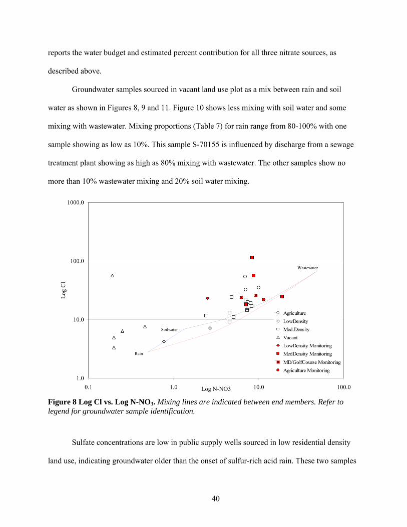
Groundwater samples sourced in vacant land use plot as a mix between rain and soil

water as shown in Figures 8, 9 and 11. Figure 10 shows less mixing with soil water and some

mixing with wastewater. Mixing proportions (Table 7) for rain range from 80-100% with one

sample showing as low as 10%. This sample S-70155 is influenced by discharge from a sewage

treatment plant showing as high as 80% mixing with wastewater. The other samples show no

more than 10% wastewater mixing and 20% soil water mixing.

Figure 8 Log Cl vs. Log N-NO3. Mixing lines are indicated between end members. Refer to legend for groundwater sample identification.

Wastewater

Rain

Soilwater

1.0

10.0

100.0

1000.0

0.1 1.0 10.0 100.0Log N-NO3

Log

Cl

A T E R

WA S T E WA T E R

AgricultureLowDensityMed.DensityVacantLowDensity Monitoring MedDensity MonitoringMD/GolfCourse MonitoringAgriculture Monitoring

Sulfate concentrations are low in public supply wells sourced in low residential density

land use, indicating groundwater older than the onset of sulfur-rich acid rain. These two samples

40

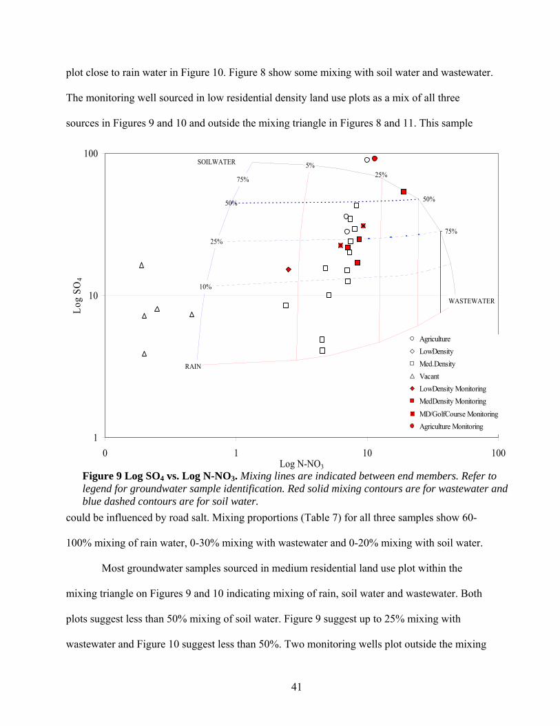
plot close to rain water in Figure 10. Figure 8 show some mixing with soil water and wastewater.

The monitoring well sourced in low residential density land use plots as a mix of all three

sources in Figures 9 and 10 and outside the mixing triangle in Figures 8 and 11. This sample

could be influenced by road salt. Mixing proportions (Table 7) for all three samples show 60-

100% mixing of rain water, 0-30% mixing with wastewater and 0-20% mixing with soil water.

RAIN

10%

75%

SOILWATER

25%

50%

75%

50%

25%5%

WASTEWATER

1

10

100

0 1 10 100Log N-NO

Log

SO4

3


Figure 9 Log SO4 vs. Log N-NO3. Mixing lines are indicated between end members. Refer to legend for groundwater sample identification. Red solid mixing contours are for wastewater and blue dashed contours are for soil water.

Most groundwater samples sourced in medium residential land use plot within the

mixing triangle on Figures 9 and 10 indicating mixing of rain, soil water and wastewater. Both

plots suggest less than 50% mixing of soil water. Figure 9 suggest up to 25% mixing with

wastewater and Figure 10 suggest less than 50%. Two monitoring wells plot outside the mixing

41

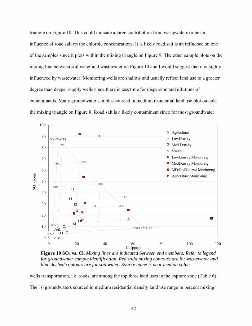
triangle on Figure 10. This could indicate a large contribution from wastewaters or be an

influence of road salt on the chloride concentrations. It is likely road salt is an influence on one

of the samples since it plots within the mixing triangle on Figure 9. The other sample plots on the

mixing line between soil water and wastewater on Figure 10 and I would suggest that it is highly

influenced by wastewater. Monitoring wells are shallow and usually reflect land use to a greater

degree than deeper supply wells since there is less time for dispersion and dilutions of

contaminants. Many groundwater samples sourced in medium residential land use plot outside

the mixing triangle on Figure 8. Road salt is a likely contaminant since for most groundwater

wells transportation, i.e. roads, are among the top three land uses in the capture zone (Table 6).

The 16 groundwaters sourced in medium residential density land use range in percent mixing.

RAIN

10%

75%

SOILWATER

50%

75%

50%

5%

WASTEWATER

25%

0

10

20

30

40

50

60

70

80

90

100

0 20 40 60 80 100 120Cl (ppm)

SO4 (

ppm

)


Figure 10 SO4 vs. Cl. Mixing lines are indicated between end members. Refer to legend for groundwater sample identification. Red solid mixing contours are for wastewater and blue dashed contours are for soil water. Source name is near median value.

42

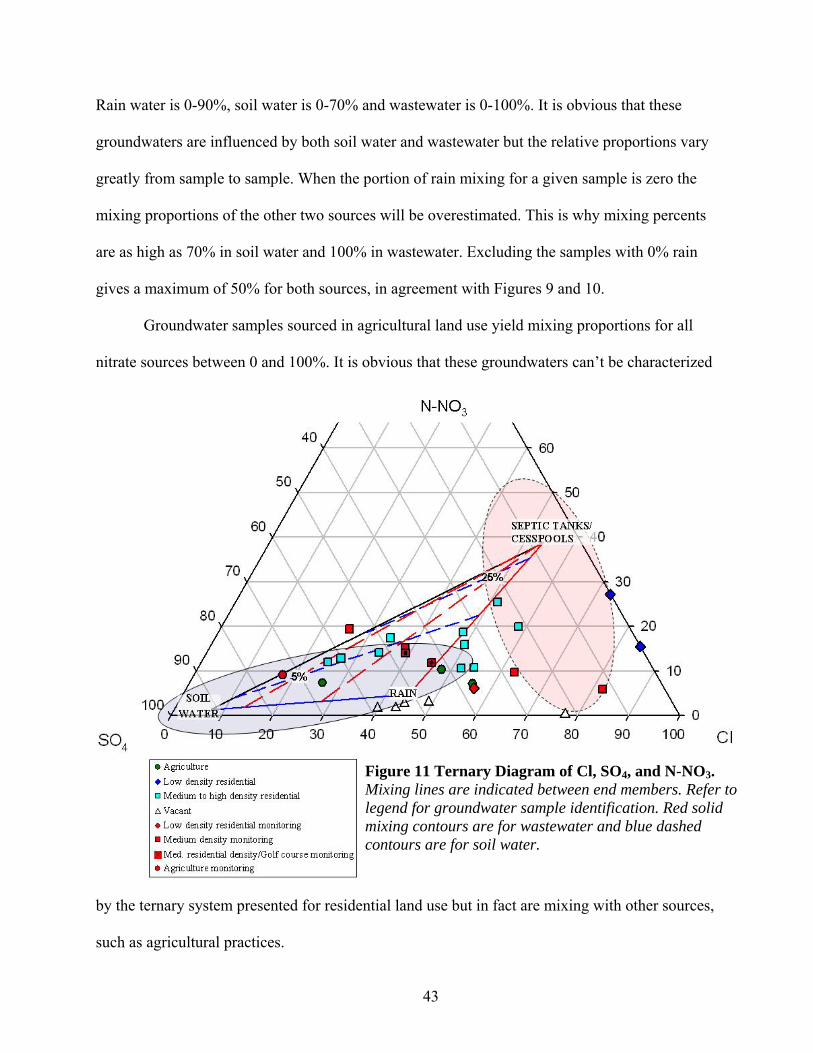
Rain water is 0-90%, soil water is 0-70% and wastewater is 0-100%. It is obvious that these

groundwaters are influenced by both soil water and wastewater but the relative proportions vary

greatly from sample to sample. When the portion of rain mixing for a given sample is zero the

mixing proportions of the other two sources will be overestimated. This is why mixing percents

are as high as 70% in soil water and 100% in wastewater. Excluding the samples with 0% rain

gives a maximum of 50% for both sources, in agreement with Figures 9 and 10.

Groundwater samples sourced in agricultural land use yield mixing proportions for all

nitrate sources between 0 and 100%. It is obvious that these groundwaters can’t be characterized

by the ternary system presented for residential land use but in fact are mixing with other sources,

such as agricultural practices.

Figure 11 Ternary Diagram of Cl, SO4, and N-NO3. Mixing lines are indicated between end members. Refer to legend for groundwater sample identification. Red solid mixing contours are for wastewater and blue dashed contours are for soil water.

43

Figure 11 is a ternary diagram of Cl, N-NO3 an

low residential land use are low in SO4 and plot on the

old groundwater (Schoonen and Brown, 1994). The gr

use plot close to rain water. Groundwater samples influ

suggest mixing of all three sources with mixing greate

water. The groundwaters sourced in agricultural land u

medium residential density land use samples.

44

d SO4. Again, groundwaters influenced by

zero SO4 contour line possibly indicating

oundwater samples sourced in vacant land

enced by residential land use would

r than 5% with wastewater and for soil

se plot close to groundwaters sourced in

iv. Conclusions

Major element data along with nitrate compositions of groundwater show a

distinct relationship between land use and sources of nitrate contamination such that the

geochemistry of groundwater associated with (1) vacant or open land use has a signature close to

rain water (2) low residential density land use is mostly influenced by rain water with some

contributions of soil water and wastewater (3) medium residential density land use plots as a

mixture of rain, soil water and wastewater and (4) agricultural land use is not distinguishable

from groundwater associated with urban land use.

These data allow estimates but do not allow precise calculations of the proportions of

rainwater, soil water and waste water in groundwater because of the rather large ranges in the

concentrations of the elements in the sources. Sulfate concentrations give the best estimate for

contributions by soil water. Nitrate concentrations give the best estimate for contributions by

wastewater. Water budgets for capture zones aid in placing constraints on mixing proportions of

nitrate sources for a given groundwater.

45

v. References

Allee, D., Raymond, L., Skaley, J., and Wilcox, D., 2001, A guide to the public management of private septic systems: Ithaca, Cornell University, p. 109.

Andreoli, A., Reynolds, R., Bartilucci, N., and Forgione, R., 1977, Pilot plant study: nitrogen removal in a modified residnetial subsurface sewage disposal system: Hauppauge, New York, Suffolk County Department of Health Services.

Barrett, M.H., Hiscock, K.M., Pedley, S., Lerner, D.N., Tellam, J.H., and French, M.J., 1999, Marker species for identifying urban groundwater recharge sources: A review and case study in Nottingham, UK: Water Research, v. 33, p. 3083-3097.

Beckerus, Rosander, Kemi, and Miljo, 1998, What effect has the eco-labelling of household detergents had on sewage treatment plants?, Swedish Society for Nature Conservation, p. 48.

Bleifuss, P.S., Hanson, G.N., and Schoonen, M., 2000, Tracing sources of nitrate in the Long Island aquifer system: on line.

Brown, C.J., and Scorca, M., 1995, Effects of road salting on stormwater and ground-water quality at the East Meadow Brook headwaters area, Nassau County, Long Island, New York, Geology of Long Island and Metropolitan New York: SUNY Stony Brook, Long Island Geologist, p. 8-20.

Buxton, H.T., and Modica, E., 1992, Patterns and rates of groundwater flow of Long Island, New York: Ground Water, v. 30, p. 857-866.

CDM, C.D.M., 2003, Long Island source water assessment summary report, New York State Department of Health, p. 53.

Elhatip, H., Afsin, M., Kuscu, I., Dirik, K., Kurmac, Y., and Kavurmac, M., 2003, Influences of human activites and agriculture on groundwater quality of Kayseri-Incesu-Dokuzpnar springs, central Anatolian part of Turkey: Environmental Geology, v. April, p. on-line.

Flipse, W.J., and Bonner, F.T., 1985, Nitrogen-Isotope Ratios of Nitrate in Ground-Water under Fertilized Fields, Long-Island, New-York: Ground Water, v. 23, p. 59-67.

Flipse, W.J., Katz, B.G., Lindner, J.B., and Markel, R., 1984, Sources of Nitrate in Groundwater in a Sewered Housing Development, Central Long Island, New-York: Ground Water, v. 22, p. 418-426.

Flynn, J.M., Padar, F.V., Guererra, A., Andres, B., and Graner, W., 1969, The Long Island ground water pollution study, State of New York Department of Health, p. 10-4.

Fuller, T., and Bova, R., 2004, Effects of road salting on ground water quality at the Suffolk County Water Authority Ackerly Pond and Mill Land well fields, Peconic, Town of Southold, Geology of Long Island and Metropolitan New York: SUNY Stony Brook, Long Island Geologist, p. http://pbisotopes.ess.sunysb.edu/lig/Conferences/abstracts-04/04_program.htm.

Gaillardet, J., Lemarchand, D., Gopel, C., and Manhes, G., 2001, Evaporation and sublimation of boric acid: Application for boron purification from organic rich solutions: Geostandards Newsletter-the Journal of Geostandards and Geoanalysis, v. 25, p. 67-75.

Gajurel, D., Li, Z., and Otterpohl, R., 2001, Newly developed medium-tech decentralised sanitation concepts for closing nutriend and water cycle, in

46

http://pbisotopes.ess.sunysb.edu/lig/Conferences/abstracts-04/04_program.htm

http://www.ias.unu.edu/proceedings/icibs/ecosan/abstracts.html, ed., Internet dialogue on ecological sanitation: A post-conference activity of the 1st International conference on ecological sanitation: Nanning, China, p. P-19.

Jonsson, H., 2001, Source seperation of human urine - seperation efficiency and effects on water emissions, crop yield, energy usage and reliability, in http://www.ias.unu.edu/proceedings/icibs/ecosan/abstracts.html, ed., Internet dialogue on ecological sanitation: A post-conference activity of the 1st International conference on ecological sanitation: Nanning, China, p. P-14.

Jonsson, H., Stenstrom, T., Svensson, J., and Sundin, A., 1997, Source separated urine-nutrient and heavy metal content, water saving and faecal contamination: Water Science and Technology, v. 35, p. 145-152.

Kolpin, D.W., Furlong, E.T., Meyer, M.T., Thurman, E.M., Zaugg, S.D., Barber, L.B., and Buxton, H.T., 2002, Pharmaceuticals, hormones, and other organic wastewater contaminants in U.S. Streams, 1999-2000: A national reconnaissance: Environ. Sci. Technol., v. 36, p. 1202-1211.

Kreitler, C.W., Ragone, S.E., and Katz, B.G., 1978, N15/N14 ratios of ground-water nitrate, Long Island, New York: Ground Water, v. 16, p. 404-409.

Langmuir, C.H., Vocke, R.D., Hanson, G.N., and Hart, S.R., 1978, A general mixing equation with applications to icelandic basalts: Planetary Science Letters, v. 37, p. 380-392.

Larsen, T., Peters, I., Alder, A., Eggen, R., Maurer, M., and Muncke, J., 2001, Re-engineering the toilet for sustainable wastewater management: Environ. Sci. Technol., v. 35, p. 192A-197A.

Leamond, C., Haefner, R., Cauller, S., and Stackelberg, P., 1992, Ground-water quality in five areas of different land use in Nassau and Suffolk counties, Long Island, New York: Syosset, New York, U.S. Geological Survey, p. 67.

Lerner, D.N., 2002, Identifying and quantifying urban recharge: a review: Hydrogeology Journal, v. 10, p. 143-152.

Ligman, K., Hutzler, N., and Boyle, W.C., 1974, Household Wastewater Characterization: Journal of the Environmental Engineering Division-Asce, v. 100, p. 201-213.

Lindberg, D.A.B., 2004, Medline Plus, Medical Encyclopedia, U.S National Library of Medicine and the National Institutes of Health: http://www.nlm.nih.gov/medlineplus/encyclopedia.html.

Mackenzie, F., 1998, Our changing planet an introduction to earth system science and global environmental change, Prentice Hall, 486 p.

Medcalf, and Eddy, 2003, Wastewater engineering: treatment and reuse, McGraw-Hill, 1819 p.

Proios, J., and Schoonen, M., 1994, The traditional chemical composition of precipitation in the Peconic River watershead, Long Island, New York, Geology of Long Island and Metropolitan New York: SUNY Stony Brook, Long Island Geologist, p. 81-85.

Renyolds, C.W., 1994, Ground water contamination from household septic systems [Masters thesis]: Stony Brook, State University of New York at Stony Brook.

Schoonen, M., and Brown, C.J., 1994, The hydrogeochemistry of the Peconic River watershed: A quantitative approach to estimate the anthropogenic loadings in the

47

http://www.ias.unu.edu/proceedings/icibs/ecosan/abstracts.html

http://www.ias.unu.edu/proceedings/icibs/ecosan/abstracts.html

http://www.nlm.nih.gov/medlineplus/encyclopedia.html

watershed, Geology of the Long Island and Metropolitan New York: SUNY Stony Brook, Long Island Geologist, p. 117-123.

Schuchman, P., 2001, The Fate of Nitrogenous Fertilizer Applied to Differing Turfgrass Systems [Masters thesis]: Stony Brook, SUNY Stony Brook.

Siegrist, R., Witt, M., and Boyle, W.C., 1976, Characteristics of Rural Household Wastewater: Journal of the Environmental Engineering Division-Asce, v. 102, p. 533-548.

Stackelberg, P., 1995, Relation between land use and quality of shallow, intermediate, and deep ground water is Nassau and Suffolk counties, Long Island, New York: Coram, New York, U.S. Geological Survey, p. 82.

Stumm, W., and Morgan, J., 1996, Aquatic chemistry: traditional chemical equilibria and rates in natural waters, Wiley-Interscience, 1022 p.

Thomas, M.A., 2000, The effects of residential development on groundwater quality near Detroit, Michigan: Journal of the American Water Resources Association, v. 36, p. 1023-1038.

Trauth, R., and Xanthopoulos, C., 1997, Non-point pollution of groundwater in urban areas: Water Research, v. 31, p. 2711-2718.

Vijst, v.d., and Groot-Marcus, 1999, Consumption and domestirc waste water demographic factors and developments in society: Water Science and Technology, v. 39, p. 41-47.

Wayland, K.G., Long, D.T., Hyndman, D.W., Pijanowski, B.C., Woodhams, S.M., and Haack, S.K., 2003, Identifying relationships between baseflow geochemistry and land use with synoptic sampling and R-mode factor analysis: Journal of Environmental Quality, v. 32, p. 180-190.

Williams, A.E., Lund, L.J., Johnson, J.A., and Kabala, Z.J., 1998, Natural and anthropogenic nitrate contamination of groundwater in a rural community, California: Environmental Science & Technology, v. 32, p. 32-39.

Wilsenach, J., and van Loosdrecht, M., 2003, Impact of separate urine collection on wastewater treatment systems: Waste Science and Technology, v. 48, p. 103-110.

48

Documents

I. CHAPTER 1 Using major elements to determine sources of