Last Modified 05/07/2015

I-5-1

I-5. Event Trees

Key Concepts

Event tree analysis is a commonly used tool in dam and levee safety risk analysis to

identify, characterize, and estimate risk. Quantitative estimates for probability of breach

or failure and the resulting consequences can be obtained using event trees. Qualitative

depictions of potential failure modes and consequences can also be developed using event

trees. Event sub trees can be used to further evaluate specific events within the overall

event tree structure. Event sub trees are typically developed for individual potential

failure modes to fully describe the sequence of events and/or conditions required to

obtain failure.

A logical progression of events is represented by the event tree beginning with an

initiating event and continuing through to a set of outcomes. A typical progression might

include an initiating event (flood or earthquake) followed by a system response (breach

or non-breach) resulting in potential consequences (life loss, economic). Additional

contributing events such as inoperable spillway gates (initiating event), flood fighting

(system response), and exposure (consequences) should also be considered in the event

tree.

An event tree consists of a sequence of interconnected nodes and branches. Each node

defines a random variable that represents an uncertain event (a crack forms in the

embankment) or state of nature (existence of adversely oriented joint planes). Branches

originating from a node represent each of the possible events or states of nature that can

occur. Probabilities are estimated for each branch to represent the likelihood for each

event or condition. These probabilities are conditional on the occurrence of the preceding

events to the left in the tree. Risks are typically annualized (e.g. probability of breach per

year or annual life loss) in the event tree by using annual probabilities to characterize the

loading conditions. The conditional structure of the event tree allows the probability for

any sequence of events to be computed by multiplying the probabilities for each branch

along a pathway. The branching structure of the event tree, which requires that all

branches originating from a node be mutually exclusive and collectively exhaustive,

allows the probability for any combination of events (e.g. total failure probability for a

potential failure mode) to be computed by summing branch probabilities across multiple

pathways.

Terminology

An example event tree structure is presented in Figure I-5-1. Terms used to describe the

event tree structure are illustrated in the figure and defined below.

I-5-2

Figure I-5-1. Event Tree Terminology

Branch – A possible event associated with a preceding chance node usually designated by

a line segment. Mathematically it represents a subset of the sample space for all possible

outcomes associated with a random variable.

Branch probability – The probability of the event represented by the branch conditioned

on the occurrence of the events to its left in the event tree.

Chance Node – A branching point in the event tree usually designated by a circle at the

end of a branch indicating the occurrence of an unknown event.

End Node – The outcome of a pathway belonging to the last level of branches in an event

tree. An end node defines a possible end state for a sequence of events.

Pathway – A unique sequence of events representing a possible set of events.

Mathematically it is the chain of random variable outcomes represented by the

intersection of the events along the pathway.

Branch Types

A branch can be used to represent different types of random variables. Terms used in the

USACE DAMRAE software to describe common variable types are summarized below.

Discrete – Discrete branch types represent discrete random variables. An example would

be a set of branches representing the number of spillway gates that are not operational.

Each discrete outcome is represented by a separate branch in the event tree.

Continuous – Continuous branch types represent continuous random variables. An

example would be a set of branches representing the annual peak water surface elevation,

with each branch representing a range of elevations.

Chance

Node

Branch

Branch

Probability

Pathway

60.0% 0.108%

5 5

0.2% Chance

0 7.8

40.0% 0.072%

12 12

90.0% Chance

0 0.0316

60.0% 0.054%

10 10

0.1% Chance

0 16

40.0% 0.036%

25 25

60.0% 53.838%

0 0

99.7% Chance

0 0

40.0% 35.892%

0 0

Chance

0.28012

60.0% 0.03%

8 8

0.5% Chance

0 12.8

40.0% 0.02%

20 20

10.0% Chance

0 2.5168

60.0% 0.018%

20 20

0.3% Chance

0 24

40.0% 0.012%

30 30

60.0% 5.952%

2 2

99.2% Chance

0 2.4

40.0% 3.968%

3 3

Example

Flood Interval 1

Flood Interval 2

Failure Mode 1

Exposure 1

Exposure 2

Failure Mode 2

Exposure 1

Exposure 2

Failure Mode 2

Exposure 1

Exposure 2

Failure Mode 1

Exposure 1

Exposure 2

Non-Breach

Exposure 1

Exposure 2

Non-Breach

Exposure 1

Exposure 2

End

Node

I-5-3

Continuous branch types need to be discretized for the event tree calculations. This can

be done manually using a spreadsheet or automatically using DAMRAE.

State Function – State function branch types represent functions or variables that are

estimated based on variables to the left in the event tree. The state function can then be

used to estimate variables to the right in the event tree. For example, the overtopping

depth might be defined as a function of the peak water surface elevation and the top of

dam elevation. The probability of failure by overtopping erosion can then be defined as a

function of overtopping depth. The use of state functions can increase transparency and

simplify changes to the event tree. For example, the event tree can be easily modified to

evaluate a dam raise alternative by simply changing the top of dam elevation in the state

function (assuming the dam raise does not change the erosion characteristics of the dam

or foundation).

Failure – Failure branch types represent a discrete random variable with only two

possible outcomes (breach or non-breach). Failure probabilities are typically defined

conditional on one or more of the loading parameters (e.g. water surface elevation or

ground acceleration).

Exposure – Exposure branch types represent a discrete random variable that is used to

characterize the fraction of time that the population at risk might be exposed to

inundation. Typical exposure scenarios might include time of day (day, night), time of

week (weekday, weekend), or time of year (summer, winter).

Intervention – Intervention branch types represent a discrete random with only two

possible outcomes (successful intervention or unsuccessful intervention).

Consequences – Consequence branch types represent a discrete random variable that is

used to characterize the magnitude of consequences (life loss, economic loss,

environmental damage). The inundation zone can be divided into multiple consequence

centers to account for differences in warning time and evacuation.

Event Tree Structure

The starting point for an event tree is a defined event (or state of nature). For dam and

levee risk analysis, this is typically a loading event such as a flood or earthquake.

Subsequent events are then defined using a divergent branching structure where each

branch represents a unique event. The branching structure is used to define all of the

possible, but unknown, events that might occur. The sequencing of events in the tree

should be logical but does not necessarily need to be chronological.

Branches and their associated branch probabilities that are statistically dependent on

preceding events must be shown along pathways to the right of the events on which they

are statistically dependent. This is an important consideration in event tree construction

because branch probabilities are mathematically defined as conditional probabilities.

This also allows branch probabilities to be a function of a state variable in a preceding

branch. The event tree in Figure I-5-2 illustrates an example where the probability of

failure is conditional on obtaining a particular water surface stage (S) during a random

flood event.

I-5-4

Figure I-5-2. Conditional Event Tree Probability

The conditional structure of the event tree satisfies the probability calculus for

statistically independent events; therefore, branch probabilities can be multiplied along a

pathway to obtain the probability for the intersection of events along the pathway. In the

preceding example, the probability of failure can be computed as P(Stage) *

P(Fail|Stage).

Branches that originate from a chance node should be mutually exclusive and collectively

exhaustive. This makes each event and pathway unique (mutually exclusive) and ensures

that all possible events and pathways are considered (collectively exhaustive). A result of

this requirement is that branch probabilities originating from a node can be summed and

the total sum across all branches must equal one. This provides a convenient validation

check for the event tree structure. This requirement is illustrated in Figure I-5-3.

Figure I-5-3. Mutually Exclusive and Collectively Exhaustive

Branch probabilities within a particular level of the event tree can be summed to obtain

an aggregate probability (or risk) associated with a set of related events. The event tree

in Figure I-5-4 illustrates the summation of potential failure mode pathway probabilities

to obtain the total probability of failure for Flood Interval 1. Total annualized life loss

can be similarly obtained by multiplying the failure probability and associated

consequences for each end branch and then summing across the end branches.

60.0% 0.108%

5 5

0.2% Chance

0 7.8

40.0% 0.072%

12 12

90.0% Chance

0 0.0316

60.0% 0.054%

10 10

0.1% Chance

0 16

40.0% 0.036%

25 25

60.0% 53.838%

0 0

99.7% Chance

0 0

40.0% 35.892%

0 0

Chance

0.28012

60.0% 0.03%

8 8

0.5% Chance

0 12.8

40.0% 0.02%

20 20

10.0% Chance

0 2.5168

60.0% 0.018%

20 20

0.3% Chance

0 24

40.0% 0.012%

30 30

60.0% 5.952%

2 2

99.2% Chance

0 2.4

40.0% 3.968%

3 3

Example

Flood Interval 1

Flood Interval 2

Failure Mode 1

Exposure 1

Exposure 2

Failure Mode 2

Exposure 1

Exposure 2

Failure Mode 2

Exposure 1

Exposure 2

Failure Mode 1

Exposure 1

Exposure 2

Non-Breach

Exposure 1

Exposure 2

Non-Breach

Exposure 1

Exposure 2

S = 1.0 S = 1.0

Flood

P(Stage)

P(Fail | Stage)

I-5-5

Figure I-5-4. Total Probability of Failure for Flood Interval 1

Potential Failure Mode Trees

It is common practice to develop detailed event trees for individual potential failure

modes to clearly identify the full sequence of steps required to obtain failure or breach.

Each identified potential failure mode is decomposed into a sequence of component

events and conditions that all must occur for the breach to develop. This ensures that due

consideration is given to each event in the failure sequence. It also supports the

identification of key issues contributing to the risk. A typical event tree structure for an

internal erosion potential failure mode is illustrated in Figure I-5-5. A challenge with

estimating probabilities for detailed event trees is remembering that each branch is

conditional on predecessor branches. For the typical internal erosion event tree, this

means that the probability estimate for the continuation branch should be based on an

assumption that the flaw already exists and initiation has already occurred even if the

probabilities for a flaw and initiation are very small. Examples and suggested event tree

structures for common potential failure modes are provided throughout this manual. The

suggested event trees should be adjusted as needed to address site specific conditions.

60.0% 0.108%

5 5

0.2% Chance

0 7.8

40.0% 0.072%

12 12

90.0% Chance

0 0.0316

60.0% 0.054%

10 10

0.1% Chance

0 16

40.0% 0.036%

25 25

60.0% 53.838%

0 0

99.7% Chance

0 0

40.0% 35.892%

0 0

Chance

0.28012

60.0% 0.03%

8 8

0.5% Chance

0 12.8

40.0% 0.02%

20 20

10.0% Chance

0 2.5168

60.0% 0.018%

20 20

0.3% Chance

0 24

40.0% 0.012%

30 30

60.0% 5.952%

2 2

99.2% Chance

0 2.4

40.0% 3.968%

3 3

Example

Flood Interval 1

Flood Interval 2

Failure Mode 1

Exposure 1

Exposure 2

Failure Mode 2

Exposure 1

Exposure 2

Failure Mode 2

Exposure 1

Exposure 2

Failure Mode 1

Exposure 1

Exposure 2

Non-Breach

Exposure 1

Exposure 2

Non-Breach

Exposure 1

Exposure 2

S = 0.003

I-5-6

Figure I-5-5. Suggested Internal Erosion Potential Failure Mode Sub Tree

System Response

System response (or probability of failure) describes the relationship between the demand

(i.e. driving forces or loads) that a system is subjected to and the capacity (i.e. resisting

forces or strength) of the system to withstand the demand. The limit state (Z) for a

system can be defined by the equation below as the difference between the capacity (R)

and demand (S).

The probability of failure or breach for a system is the probability that the capacity is less

than or equal to the demand, P(R≤S), or the probability that the limit state is less than or

equal to zero, P(Z≤0).

The factor of safety can be defined by the equation below as the ratio of capacity to

demand.

The probability of failure or breach for a system is the probability that the factor of safety

is less than or equal to one (FS≤1). Depending on the method of analysis, a factor of

safety less than one may or may not be the most appropriate limit state for estimating the

probability of failure. The analyst must be mindful of the fact that all analytical methods

and models are only simplified approximations of reality. Some analytical methods may

be more conservative than others in their formulation and assumptions.

Evaluation of system response is a bit more mathematically cumbersome with the factor

of safety formulation because of the ratio. For this reason, the limit state formulation

Flaw ?

Initiation?

Continuation?

Progression?

Unsuccessful Intervention?

Breach?

Internal Erosion

No

Yes

No

Yes

No

Yes

No

Yes

No

Yes

No

Yes

I-5-7

expressed as the difference between capacity and demand will be used for purposes of

this section.

Both the demand and capacity are uncertain; however, system response is typically

evaluated assuming the demand is known. Uncertainties in the demand can be evaluated

in the loading branches of the event tree separately from the potential failure mode

branches. If the demand is assumed to be known, then the conditional probability of

failure or breach for a given load can be defined by the equation below where fR(r) is the

probability density function for capacity and FR(s) is the cumulative distribution function

for capacity.

The cumulative distribution function for the capacity of the system provides the

conditional probability of failure or breach for a specified demand. The probability of

failure or breach for a given demand is the probability that the capacity is less than or

equal to the demand. This means that the probability of failure or breach is the

probability that failure or breach will occur at a loading that is less than or equal to the

specified loading. The cumulative distribution function characteristic of the system

response is important to understand because system response is often incorrectly

interpreted to be the probability of failure or breach given the load instead of the

probability that failure will occur at a load less than or equal to the given load. This can

be a factor to consider during event tree analysis because event trees are typically

constructed to assume that failure or breach occurs at the peak load. In some situations,

the event tree structure may need to be modified to account for the possibility that failure

or breach can occur at a load less than the peak load during loading events with a

temporal component such as floods and earthquakes. Refer to Chapter 35 – Combining

and Portraying Risks – System Response for an example.

System Response Curves

When system response is evaluated over a range of loads, the resulting relationship is

called a system response curve. Other terms describing this relationship, such as a

‘fragility curve’, may be found in other literature. The term ‘fragility’ is intentionally not

used in this manual for dam and levee safety due to the negative connotation that results

from referring to a dam or levee as being ‘fragile’.

Potential failure mode sub trees can be used to develop system response curves that

describe the probability of failure or breach as a function of one or more loading

parameters such as peak water surface elevation or peak ground acceleration. The failure

mode event tree is evaluated for multiple loading scenarios. Branch probabilities that are

dependent on the magnitude of the load are modified for each loading scenario. These

probabilities can be estimated for the nodes of a potential failure mode sub tree using a

combination of analytical, empirical, and subjective methods. The number and spacing

of load scenarios should be sufficient to describe the shape of the system response curve

over the full spectrum of potential loads paying careful attention to transitions in system

behavior. It is important to identify and include inflection points in the system response

I-5-8

curve that represent significant changes in system behavior. A curve can be fit to the

resulting data from each of the potential failure mode sub trees so that the probability of

failure can be estimated for any load condition by interpolation. An example system

response curve is presented in Figure I-5-6.

Figure I-5-6. System Response Curve

Consequence Trees

Detailed event trees can be developed for consequence scenarios. These event trees

typically include exposure scenarios to clearly identify the conditions that could lead to

different magnitudes of consequences. This ensures that due consideration is given to the

factors that may influence consequences. It also supports the identification of the key

issues contributing to the risk. A suggested event tree structure for exposure is illustrated

in Figure I-5-7. The suggested structure proceeds from the longest exposure case

(season) toward the left of the tree to the shortest exposure case (time of day) toward the

right of the tree so that the overall size of the event tree is minimized. This example

reflects estimation of non-breach consequences. Reclamation typically does not evaluate

non-breach consequences but the structure of the example event tree would also apply to

breach consequences.

0

1Sy

ste

m R

esp

on

se P

rob

abili

ty

Load Magnitude

Curve Fit

Analysis Points

I-5-9

Figure I-5-7. Suggested Consequence Sub Tree

Event Tree Construction

Each branch in the event tree should be clearly defined and representative of a specific

event or state of nature. Parallel components can be aggregated into a single event if

different combinations are inconsequential to the risk analysis. For example, it might be

sufficient to represent failure of a spillway gate in one branch if it doesn’t matter which

particular spillway gate fails. Events that could influence other system components

should generally be toward the left of the event tree to reduce the overall tree size.

Constructing the event tree in chronological order is not required mathematically, but it

usually improves the logic which can facilitate understanding and communication. The

event tree structure should be designed to accommodate future needs such as the

evaluation of risk reduction alternatives to minimize duplication of effort and provide

consistency in the risk estimates across multiple phases of study. Avoid detailed

development of branches that do not lead to outcomes important to the risk estimate or

risk management decisions. Care should also be taken to avoid situations where the risk

becomes a function of the number of branches in the event tree (i.e. adding more

branches to obtain a lower risk estimate). Multiple branch levels can be combined into a

single branch level when the added resolution does not significantly improve the

understanding, estimation, or portrayal of risks. Events with relatively low and

inconsequential probabilities can also be excluded from the event tree. Care should be

taken to avoid underestimating the risk if many branches are excluded or if the excluded

branches could be important to follow on risk estimates (e.g. alternative evaluation).

I-5-10

Common Cause Adjustment

Full enumeration of all possible events in an event tree can become unwieldy and is

usually unnecessary.

Consider a dam with the following three seismic induced potential failure modes: A)

sliding within the foundation of a concrete gravity monolith, B) buckling of a spillway

gate arm, and C) liquefaction of the foundation leading to crest deformation and

overtopping. The probability of failure for each of these potential failure modes has been

estimated assuming the potential failure modes are statistically independent.

P(A) = 0.3

P(B) = 0.1

P(C) = 0.2

A total of seven permutations might be obtained from combinations of the three potential

failure modes plus one permutation for the non-breach outcome. These permutations are

mutually exclusive and collectively exhaustive. The permutations are listed below and

depicted in the Venn diagram in Figure I-5-8.

1. Breach by A only {A, B , C }

2. Breach by B only {A , B, C }

3. Breach by C only {A , B , C}

4. Breach by A and B {A, B, C }

5. Breach by A and C {A, B , C}

6. Breach by B and C {A , B, C}

7. Breach by A, B, and C {A, B, C}

8. Non-breach {A , B , C }

Figure I-5-8. Venn Diagram for Potential Failure Mode Permutations

{A , B , C }

{A, B , C } {A , B, C }

{A , B , C}

{A , B, C}

{A, B, C }

{A, B , C}

{A, B, C}

I-5-11

The probability for each permutation can be computed as the intersection of the three

events within each permutation by multiplying the underlying probabilities (assuming

that A, B, and C are statistically independent). The probabilities for permutations that

include a breach can then be summed to obtain the total probability of breach for the

system. Note that the probability of a potential failure mode not occurring is equal to one

minus the probability of breach [ P(A ) = 1- P(A)].

1. P(A ∩ B ∩ C ) = 0.3 * 0.9 * 0.8 = 0.216

2. P(A ∩ B ∩ C ) = 0.7 * 0.1 * 0.8 = 0.056

3. P(A ∩ B ∩ C) = 0.7 * 0.9 * 0.2 = 0.126

4. P(A ∩ B ∩ C ) = 0.3 * 0.1 * 0.8 = 0.024

5. P(A ∩ B ∩ C) = 0.3 * 0.9 * 0.2 = 0.054

6. P(A ∩ B ∩ C) = 0.7 * 0.1 * 0.2 = 0.014

7. P(A ∩ B ∩ C) = 0.3 * 0.1 * 0.2 = 0.006

8. P(A ∩ B ∩ C ) = 0.7 * 0.9 * 0.8 = 0.504

The total probability of breach is equal to

0.216 + 0.056 + 0.126 + 0.024 + 0.054 + 0.014 + 0.006 = 0.496

This result is the same as the estimate that can be obtained using deMorgan’s rule.

The total probability of non-breach is equal to the probability for permutation number

eight or it can be estimated as one minus the total probability of breach.

1 - 0.496 = 0.504

As a check, note that the sum of the probabilities for breach and non-breach is equal to

one which satisfies the probability calculus for mutually exclusive and collectively

exhaustive events.

A complete event tree would include each of the possible permutations and their

associated probabilities. The probabilities for each permutation can be directly applied

with no adjustment, if every permutation is explicitly enumerated as a separate branch in

the event tree. The probabilities for the branches can be summed because the branches

satisfy the requirement of being mutually exclusive and collectively exhaustive. Event

tree branches for the eight permutations in the example are illustrated in Figure I-5-9.

I-5-12

Figure I-5-9. Potential Failure Mode Permutations

The number of event tree branches can quickly become unwieldy in a risk analysis if all

permutations are enumerated. When scenarios with multiple breaches are included,

attribution of the risk back to the individual potential failure modes can be confusing for

both the risk analyst and the decision maker. Fortunately, there are some logical steps

that can be taken to simplify the event tree structure. If the occurrence of multiple

breaches is unlikely, then these permutations can be eliminated from the event tree. For

dams, this is often a reasonable assumption given that the reservoir is likely to drain

quickly following initiation of the first potential failure mode. The subsequent reduction

in load makes the initiation of additional potential failure modes unlikely. The chance for

two potential failure modes occurring simultaneously on dam is usually remote. For

levees, initiation of the first potential failure mode may lead to flooding of the leveed area

which can reduce the differential load thus reducing the potential for initiation of

additional failure modes. This assumption may not be reasonable for long levees with

large leveed areas that are subjected to long duration events. In these situations the load

may not be reduced by a single breach of the levee and subsequent breaches may be

plausible because the load occurs over a long duration or flooding of the leveed area does

not reduce the differential load. Permutations with multiple breaches can also be

eliminated when the consequences due to multiple breaches are not significantly different

than the consequences due to a single breach. This may be a reasonable assumption for

dams if the first failure inundates the entire downstream floodplain or for levees if the

first failure floods the leveed area.

From the previous example, the following four permutations would remain if multiple

breaches are believed to be unlikely and/or inconsequential to the risk estimate.

1. Breach by A only {A, B , C }

2. Breach by B only {A , B, C }

3. Breach by C only {A , B , C}

4. Non-breach {A , B , C }

)126.0(},,{ CBA

)024.0(},,{ CBA

)054.0(},,{ CBA

)504.0(},,{ CBA

)056.0(},,{ CBA

)216.0(},,{ CBA

)014.0(},,{ CBA

)006.0(},,{ CBA

I-5-13

Trimming event tree branches in this manner requires that the probabilities associated

with the branches containing multiple breaches be allocated back to the remaining

branches associated with the individual potential failure modes. This must be done to

maintain the correct total probability and to ensure that the remaining events will be

mutually exclusive and collectively exhaustive. In the Venn diagram, this is equivalent

to allocating the overlapping areas back to the individual potential failure mode

outcomes. Allocation of the overlapping areas is illustrated in Figure I-5-10.

Figure I-5-10. Allocating Multiple Breaches to Individual Potential Failure Modes

Hill et al (2003) have proposed a simplified approach for allocating the probabilities

associated with the overlapping areas back to the individual potential failure modes. This

is the method used by both Reclamation and USACE. The method distributes the

overlapping area proportional to the probability of failure for each potential failure mode.

Larger probabilities of failure receive a larger portion of the overlapping area. The

approach is implemented using the following equation where is the unadjusted

probability of failure for potential failure mode j and is the adjusted probability of

failure.

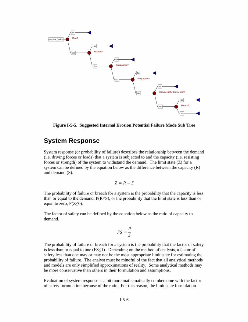
For the example, the adjusted probabilities of failure are

{A , B , C }

{A, B , C } {A , B, C }

{A , B , C}

I-5-14

The sum of the adjusted probabilities is now equal to the correct total probability of

failure

0.248 + 0.083 + 0.165 = 0.496

The adjusted probabilities can now be used in a pruned event tree that includes the three

individual potential failure mode permutations and the non-breach permutation. The

pruned event tree is illustrated in Figure I-5-11.

Figure I-5-11. Event Tree After Pruning

An alternative method for allocating the overlapping area back to the individual potential

failure modes would be to explicitly decide how much of the overlapping area to allocate

to each potential failure mode permutation. One approach might be to distribute the

overlaps equally among the contributing potential failure modes based on an assumption

that each potential failure mode is equally likely to initiate first. We start with the same

eight permutations previously developed for the seismic potential failure mode example.

1. P(A ∩ B ∩ C ) = 0.3 * 0.9 * 0.8 = 0.216

2. P(A ∩ B ∩ C ) = 0.7 * 0.1 * 0.8 = 0.056

3. P(A ∩ B ∩ C) = 0.7 * 0.9 * 0.2 = 0.126

4. P(A ∩ B ∩ C ) = 0.3 * 0.1 * 0.8 = 0.024

5. P(A ∩ B ∩ C) = 0.3 * 0.9 * 0.2 = 0.054

6. P(A ∩ B ∩ C) = 0.7 * 0.1 * 0.2 = 0.014

7. P(A ∩ B ∩ C) = 0.3 * 0.1 * 0.2 = 0.006

8. P(A ∩ B ∩ C ) = 0.7 * 0.9 * 0.8 = 0.504

The overlap is then equally distributed among the contributing potential failure modes.

1. P(A) = P(A ∩ B ∩ C ) + 1/2 P(A ∩ B ∩ C ) + 1/2 P(A ∩ B ∩ C) + 1/3 P(A ∩ B ∩ C) = 0.257

2. P(B) = P(A ∩ B ∩ C ) + 1/2 P(A ∩ B ∩ C ) + 1/2 P(A ∩ B ∩ C) + 1/3 P(A ∩ B ∩ C) = 0.077

3. P(C) = P(A ∩ B ∩ C) + 1/2 P(A ∩ B ∩ C) + 1/2 P(A ∩ B ∩ C) + 1/3 P(A ∩ B ∩ C ) = 0.162

The sum of the adjusted probabilities is now equal to the correct total probability of

failure.

)248.0(},,{ CBA

)083.0(},,{ CBA

)165.0(},,{ CBA

)504.0(},,{ CBA

I-5-15

0.257 + 0.077 + 0.162 = 0.496

Note that different methods will result in different adjusted probability values. It is

important that the facilitator documents the methods and assumptions that are used to

adjust probabilities.

Hill et al (2003) recommend freezing the adjusted probability values when a dam or levee

is estimated to fail prior to a possible higher loading condition to avoid unrealistic

adjustments for potential failure modes at the higher loads. The adjusted probabilities are

frozen at the first loading interval for which an unadjusted probability equals one.

Freezing is suggested for flood loading scenarios because the load develops gradually

such that the dam would fail prior to reaching the higher load condition. Freezing is not

suggested for seismic potential failure modes because the load develops more rapidly

such that peak load conditions can still be obtained prior to failure. Consequence

estimates can also be frozen in a similar manner to avoid unrealistic consequences for

flood events greater than the event at which the dam is expected to fail. Figure I-5-12

illustrates the freezing concept applied to two system response curves.

Figure I-5-12. Probability Adjustment Without and With Freezing

Partitioning

Event trees are comprised of a discrete number of branches. For flood and seismic loads,

a suggested approach is to divide the loading into discrete intervals. The probability for a

load interval can be computed from the exceedance probability curve as the difference

between the exceedance probabilities at the upper and lower bound of the interval. A

representative index value can be estimated for each loading interval. The index value is

typically estimated as an average of the upper and lower bound values. For flood and

seismic loading intervals, the geometric mean (obtained by taking the square root of the

product of the upper and lower bound probabilities) is suggested as a reasonable

representative value because these random variables tend to be lognormally distributed.

The partitioning concept is illustrated in Figure I-5-13.

0

1

Syst

em R

esp

on

se P

rob

abili

ty

Water Surface Elevation

Unadjusted

Adjusted With Freezing

0

1

Syst

em R

esp

on

se P

rob

abili

ty

Water Surface Elevation

Unadjusted

Adjusted Without Freezing

I-5-16

Figure I-5-13. Event Tree Load Intervals

Index points can be used in subsequent event tree branches to estimate probability of

failure and consequences for each interval. The number and spacing of the intervals

affects the numerical precision of the risk estimate. The objective is to define enough

intervals at a spacing that adequately characterizes the shapes of the various event tree

input functions. More intervals will improve numerical precision, but can increase the

event tree size and computation burden. When a large number of intervals are used, end

branches can be aggregated into logical bins by summation to facilitate interpretation and

communication of results. An examination of event tree probabilities such as probability

of failure and other values such as consequences at both the lower and upper bounds of

each interval can provide insights as to whether or not the intervals are appropriately

sized. A significant change from the lower to the upper bound might indicate a need for

more intervals.

The partitions should also consider a non-exceedance and an exceedance interval. The

non-exceedance interval can be established based on a threshold loading below which the

probability of failure and consequences are negligible. This becomes the bottom end of

the lowest load range for which risks are estimated. The lower bound for the non-

exceedance interval should be an annual exceedance probability of 1 and the upper bound

should be defined by the threshold event. While simple in concept, the selected threshold

value can have a significant influence on the estimated risks. Sensitivity analysis is

suggested to evaluate whether refinement of the selected threshold is needed. The

exceedance interval establishes the largest loading condition for which risks are

estimated. It is important to assess whether or not there are any significant risks

attributable to extreme loading that may be associated with high probabilities of failure.

Would the risk significantly change if an additional higher loading interval was added to

the analysis? If agency policy establishes an upper bound for loading (e.g. probable

maximum flood), then the exceedance interval can be defined based on policy. The

Interval

Index Value

Non-Exceedance Interval

Exceedance Interval

Flood Intervals

EL 1671.5, P=0.5

EL 1673.5, P=0.4

EL 1679.2, P=0.09

EL 1685.5, P=0.009

EL 1691.5, P=0.0009

EL 1695.0, P=0.0001

Lower Bound Upper Bound Index Value Lower Bound Upper Bound Probability

n/a 1671.5 1671.5 1 0.5 0.5

1671.5 1675.5 1673.5 0.5 0.1 0.4

1675.5 1683.0 1679.2 0.1 0.01 0.09

1683.0 1688.0 1685.5 0.01 0.001 0.009

1688.0 1695.0 1691.5 0.001 0.0001 0.0009

1695.0 n/a 1695.0 0.0001 0 0.0001

Elevation Probability

I-5-17

lower bound for the exceedance interval is the threshold for the largest loading that will

be considered and the upper bound should be an annual exceedance probability of zero.

Intervention

Intervention includes those actions that can lead to preventing a breach from occurring or

mitigating the consequences of a breach. Successful intervention requires taking actions

to detect a developing failure mode and then taking actions to stop further development

of the failure mode. Two phases of intervention are typically considered for possible

inclusion in the event tree. The first phase of intervention includes routine and non-

routine actions such as surveillance, inspection, monitoring, instrumentation, and flood

fighting. The first phase includes the increased surveillance and monitoring activities

that normally occur during flood events, or that could be implemented in response to

unexpected performance. Some of the flood fighting activities that might be consistent

with the first phase of intervention include actions like sandbagging boils, constructing

filters, constructing stability berms, and repairing shallow slope failures. These actions

occur during the early stages of failure mode development when development to breach

is not certain and/or may take a long time (weeks to years). Actions to prevent breach

during the first phase of intervention generally have a higher likelihood of success. The

second phase of intervention includes emergency actions that are taken as a last ditch

effort to prevent breach. These emergency actions occur during the later stages of failure

mode development when development to breach is virtually certain and imminent (hours

to days). The second phase includes things like dumping erosion resistant materials to

slow the advancement of a headcut, intentional breaching of the system in a less

damaging location to reduce consequences, or maximizing releases from a reservoir to

stop or slow progression of a failure mode in progress, or slow breach development and

reduce consequences. Actions to prevent breach during the second phase of intervention

generally have a lower likelihood of success.

Some questions to consider when evaluating intervention include:

What methods are available for detecting failure modes?

Are the detection methods appropriate for the failure mode being

evaluated?

Are the monitoring instruments appropriate?

Are the instruments maintained and in good working order?

Are the instrument indicators/thresholds appropriate?

How often is the instrumentation data evaluated?

How often are inspections conducted?

Are the personnel conducting the inspections and/or interpreting

instrument data trained to detect failure modes?

What methods are available to arrest failure mode development?

What methods have been successful in the past?

What methods have been unsuccessful in the past?

Are resources available (manpower, equipment, materials)?

Is there enough time for detection and action?

Intervention actions can be included in the event tree in a variety of ways depending on

the fidelity needed in the risk analysis. A common approach is to aggregate intervention

actions into a single event tree branch. When more resolution is needed, separate

I-5-18

branches can be included for each intervention phase. This allows a distinction to be

made between actions that are more likely to be successful (first phase) and actions that

are less likely to be successful (second phase). The probability of successful intervention

may also be easier to estimate if the two phases are considered separately.

Uncertainty

Risk estimates should give due consideration for uncertainty and sensitivity. Two

important questions to consider when evaluating and communicating uncertainty are:

Does the uncertainty significantly impact the decision?

Can the uncertainty be reduced?

Key areas of uncertainty and sensitivity should be identified and portrayed. This can be

accomplished using a variety of qualitative and quantitative techniques. Most of the

techniques used in event tree analysis are quantitative.

Sensitivity analysis can be used to evaluate how different assumptions influence the risk

estimate. It provides a way to evaluate alternative outcomes if a situation turns out to be

different than anticipated. Evaluation of the alternative outcomes can facilitate the

identification of key assumptions and the potential value added by additional study. For

example, investigations to assess the slip rate for a fault may not be justified if the risk

estimate is not sensitive to this parameter or if the uncertainty in the risk estimate will not

be reduced. Reasonable best case and reasonable worst case assumptions can be used as

a starting point for the sensitivity analysis. Sensitivity analysis typically only considers a

limited number of parameters for each scenario. Combining worst (or best) case

assumptions for all parameters are not recommended because the probability that all

parameters are unfavorable (or favorable) is usually remote.

Uncertainty analysis can be accomplished by using probability distributions to define

event tree variables. This is done to characterize the knowledge uncertainty in the event

tree inputs. This uncertainty can, at least in theory, be reduced by acquiring more

information. Distributions that are commonly used in dam and levee safety risk analysis

include uniform, triangular, normal, and log-normal. The distributions can be applied to

variables such as peak reservoir stage, peak ground acceleration, probability of failure,

and consequences. Monte carlo simulation techniques can be used to generate random

samples from these distributions. Probabilities and risks are calculated for many random

samples (typically 10,000 or more) to characterize the uncertainty in the risk estimate. It

is not always practical or possible to quantify all sources of uncertainty; therefore, it is

important to document the significant uncertainties that were included in the event tree

analysis and those that were not included.

Natural variability (aleatory uncertainty) associated with random events such as floods or

earthquakes is typically accounted for in the event tree by considering the full range of

plausible events along with their associated probability of occurrence. This is the most

common technique used by USACE and Reclamation for dam and levee risk analysis.

An alternative technique would be to develop and run a simulation model that randomly

selects a flood or earthquake event for each year of the simulation. Many years can be

simulated to capture the full range of possible loading events.

I-5-19

Monte Carlo Simulation

Monte Carlo simulation is a mathematical technique that is used to evaluate uncertainty

in risk analysis. It provides a means to evaluate the uncertainty in a risk estimate by

combining the uncertainties for all of the event tree inputs. Commercial software such as

@Risk, Crystal Ball, and many others can be used to perform the calculations. A monte

carlo simulation samples a possible value for each random variable in an event tree based

on its probability distribution. A variety of sampling methods are available. One

approach is to sample a random number that is greater than or equal to zero and less than

or equal to one. A separate random number is generated for each random variable in the

analysis. The random number can then be applied to the cumulative distribution function

as a cumulative probability to obtain a sample value for the random variable. If enough

samples are taken, the resulting distribution of the random variable samples will exactly

match the probability distribution from which the values were sampled.

Each sample produces a single estimate of the risk. The sampling process is repeated

many times to obtain many estimates of the risk. If enough samples are taken, the

sampled estimates of risk can be used to portray a probability distribution of the risk. It is

not uncommon in dam and levee safety risk analysis that 10,000 or more samples are

required to obtain a reasonable result. The sampled estimates of risk can be portrayed in

various ways to assess and communicate the uncertainty in the risk estimate. A common

approach is to show each sampled risk estimate as a point on the f-N chart along with the

mean value of the risk samples. The resulting cloud of points can provide risk analysts

and decision makers with information on the magnitude of uncertainty. Confidence

intervals can also be estimated from the sampled risk estimates to characterize the

probability that the risk estimate will fall either above or below risk guidelines.

Consider the following example for a potential failure mode that could initiate at flood

loadings greater than a 10 year flood. The conditional probability of failure was

estimated by expert elicitation and the uncertainty in the estimate is described by a

triangular distribution with a lower bound of 0.00001, an upper bound of 0.0005, and a

best estimate (mode) of 0.0002. Potential life loss was estimated from an analytical

model and the uncertainty in the estimate is described by a triangular distribution with a

lower bound of 60, an upper bound of 120, and a best estimate (mode) of 80. An event

tree with supporting spreadsheet calculations is illustrated in Figure I-5-14.

PrecisionTree and @Risk were used to develop the event tree and perform the monte

carlo simulation calculations. The PrecisionTree model settings for @Risk simulation

were set to ‘expected values of the model’ as illustrated in Figure I-5-15. The

conditional probability of failure and consequences were input using the ‘define

distribution’ feature in @Risk. The annual probability of failure (e.g. value of ‘f’ for the

f-N chart) is equal to the total probability along the breach pathway obtained by

multiplying the probability of the flood by the probability of failure. The value of ‘N’ for

the f-N chart is simply the life loss associated with a breach.

I-5-20

Figure I-5-14. Event Tree for Monte Carlo Simulation Example

Figure I-5-15. Precision Tree Settings for Monte Carlo Simulation Example

A 1000 iteration monte carlo simulation was performed on the event tree using @Risk.

The results are presented on the f-N chart in Figure I-5-16. The mean estimate was

obtained by taking the arithmetic average of the monte carlo simulation results. The best

estimate was obtained by using the best estimate values shown in Figure I-5-14.

Although the monte carlo simulation results straddle the risk guidelines, both the mean

estimate and best estimate are above the guidelines. It is important to know that the mean

risk estimate from a monte carlo simulation will often be different than the risk estimate

obtained from best estimate values. By counting the number of monte carlo simulation

results that are above the guidelines (874) and dividing by the total number of monte

carlo simulations (1000), the risk analyst might conclude that there is a relatively high

degree of confidence (about 87%) that the risk exceeds the guidelines.

I-5-21

Figure I-5-16. Monte Carlo Simulation Results

Consistent Percentile Method

Typical monte carlo simulations include the sampling of values for multiple random

variables. It is important that the sampling technique produces numbers in the event tree

that are internally consistent and logical. Consider a simple event tree with two flood

loading partitions and one potential failure mode. If the probabilities of failure are

independently sampled for each loading partition, it is possible that, for a particular

iteration, the probability of failure sampled for the smaller load partition can be greater

than the probability of failure sampled for the larger load partition. This results in an

internal inconsistency because the probability of failure should logically increase as the

load increases. The end result is that the uncertainty portrayed by the monte carlo

simulation results may not be correct and could potentially misinform decision makers.

Similar issues can occur with random variables in other event tree branches. For

example, independent sampling of flood or seismic loading parameters can cause internal

consistency errors. A peak ground acceleration that is sampled for a smaller load

partition could end up being greater than the peak ground acceleration that is sampled for

a larger load partition.

The consistent percentile method is one technique to improve internal consistency during

a monte carlo simulation. With this method, a random sample is obtained for an entire

relationship such as a flood or seismic hazard curve. A random number greater than or

equal to zero and less than or equal to one is generated for each iteration of a simulation.

This random number represents a random sample of a percentile or confidence limit

value associated with the random variable. This percentile can be applied to the

uncertainty distribution about the relationship to obtain a random sample of the curve.

1.E-07

1.E-06

1.E-05

1.E-04

1.E-03

10 100 1000

An

nu

al P

rob

abili

ty o

f Fa

ilure

, f

Life Loss, N

Monte Carlo Simulation Results

Mean Estimate

Best Estimate

I-5-22

Consider an example where the mean seismic hazard is described by the relationship in

Figure I-5-17. The uncertainty is characterized by the 5th, 16

th, 50

th, 84

th, and 95

th

percentile curves.

Figure I-5-17. Seismic Hazard Curves

The risk analyst has decided to partition the loading for the event tree based on peak

ground acceleration using the bins summarized in Table I-5-1. As a result, the seismic

hazard curves need to be extended to the maximum PGA value of 0.7 so that annual

exceedance probabilities can be obtained for each partition and for each percentile. After

consulting with the project seismologist, the extended curves presented in Figure I-5-18

are obtained.

I-5-23

Table I-5-1. Seismic Loading Partitions

Partition Lower Bound

(PGA)

Upper Bound

(PGA)

1 0 0.03

2 0.03 0.08

3 0.08 0.2

4 0.2 0.4

5 0.4 0.7

6 0.7 n/a

Figure I-5-18. Extended Seismic Hazard Curves

Annual exceedance probability values are then tabulated for each percentile at each of the

bounding pga values. The concept is illustrated in Figure I-5-19 for a PGA bounding

value of 0.2g and the results for all of the bounding pga values are summarized in Table

I-5-2.

1.E-09

1.E-08

1.E-07

1.E-06

1.E-05

1.E-04

1.E-03

1.E-02

1.E-01

1.E+00

0 0.2 0.4 0.6 0.8

An

nu

al E

xce

edan

ce P

rob

abili

ty

Peak Ground Acceleration (g)

5th and 95th Percentile

15th and 85th Percentile

50th Percentile

I-5-24

Figure I-5-19. AEP Values for 0.2g Bounding Value

Table I-5-2. Summary of AEP for Each Percentile at Bounding PGA Values

PGA AEP 5th AEP 16th AEP 50th AEP 84th AEP 95th

0.03 5.04E-03 6.31E-03 7.78E-03 1.00E-02 1.43E-02

0.08 4.90E-04 7.43E-04 1.04E-03 2.63E-03 3.48E-03

0.2 2.62E-05 5.80E-05 9.87E-05 2.36E-04 4.32E-04

0.4 6.01E-07 3.56E-06 7.32E-06 2.54E-05 6.24E-05

0.7 2.09E-09 5.34E-08 1.48E-07 1.58E-06 8.47E-06

The tabulated values are used to develop a probability distribution of AEP for each of the

bounding pga values. This can be accomplished by simply using the percentile values

from the table and interpolating for intermediate percentile values. Another option is to

fit a distribution to the percentile data. In either case, the risk analyst must make some

assumptions to ensure that the AEPs are always greater than or equal to zero at the 0

percentile and always less than or equal to one at the 100 percentile.

In this example, the @Risk software is used to fit an analytical distribution to the

percentile data using the ‘Cumulative (X,P) Points’ type in the ‘Fit Distributions to Data’

function. The risk analyst needs to select and appropriate distribution based on

experience and the characteristics of the data. A log normal distribution is selected as a

1.E-09

1.E-08

1.E-07

1.E-06

1.E-05

1.E-04

1.E-03

1.E-02

1.E-01

1.E+00

0 0.2 0.4 0.6 0.8

An

nu

al E

xce

edan

ce P

rob

abili

ty

Peak Ground Acceleration (g)

5th and 95th Percentile

15th and 85th Percentile

50th Percentile

I-5-25

reasonable fit to the data for this example based on judgment and visual inspection of the

distribution fitting results. Selection of the log-normal distribution ensures that the

sampled AEP values will always be greater than or equal to zero. The fitted distribution

can be truncated at an AEP of 1 to ensure that sampled AEP values will always be less

than or equal to one. The fitted distribution for a pga of 0.2g is illustrated in Figure I-5-

20. Parameters for the fitted distributions at each of the bounding pga values are

summarized in Table I-5-3.

Figure I-5-20. Log Normal Distribution Fit for 0.2g

Table I-5-3. Summary of Parameters for Log Normal Distribution Fit

PGA Mean AEP Standard

Deviation of AEP

0.03 8.08E-03 1.97E-03

0.08 1.46E-03 1.02E-03

0.2 1.41E-04 1.22E-04

0.4 1.43E-05 2.01E-05

0.7 1.14E-06 6.13E-06

The event tree in Figure I-5-21 has been set up using PrecisionTree and @Risk to

perform the consistent percentile calculations for this example. Sample equations are

shown to illustrate the calculation procedure. The ‘RiskUniform’ distribution is used to

sample a single random percentile value. The random percentile is applied to each of the

PGA bounding values so that a consistent set of AEP values can be obtained. The

‘RiskLognorm’ distribution is used to define the AEP distribution for each PGA

bounding value using the parameters in Table I-5-2. An AEP value at each PGA

bounding value is calculated for the random percentile based on the AEP distribution.

This is accomplished using the ‘RiskTheoPercentile’ function. The resulting random

AEP values are then applied to the load partitions in the event tree. The probability for a

partition is obtained by subtracting the AEP at the upper bound from the AEP at the

lower bound. Results for a 10,000 iteration @Risk simulation are summarized in Figure

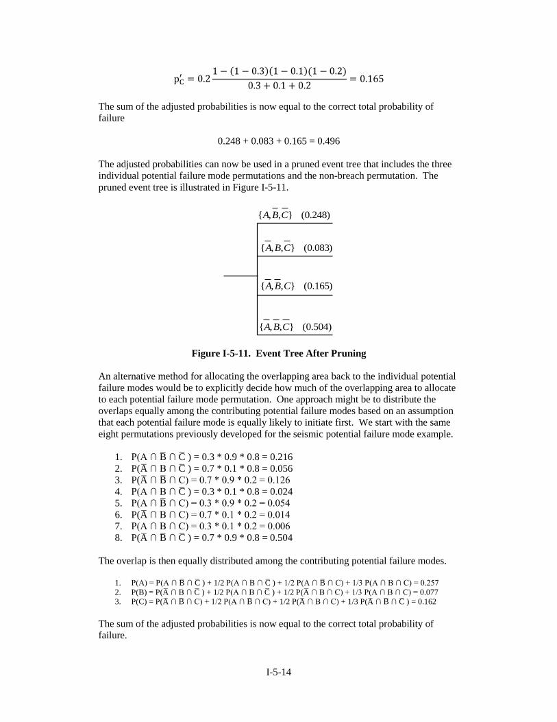
I-5-22. The distribution of the randomly sampled AEPs for the 0.2g bounding PGA value

is shown to demonstrate that the model reproduced the distribution in Figure I-5-20.

0

2000

4000

6000

8000

10000

0.E+00 1.E-04 2.E-04 3.E-04 4.E-04 5.E-04 6.E-04 7.E-04

Pro

bab

ility

De

nsi

ty

Annual Exceedance Probability for 0.2g

Log Normal Distribution Fit

Data

0

0.2

0.4

0.6

0.8

1

0.E+00 1.E-04 2.E-04 3.E-04 4.E-04 5.E-04 6.E-04 7.E-04

Cu

mu

lati

ve D

istr

ibu

tio

n

Annual Exceedance Probability for 0.2g

Log Normal Distribution Fit

Data

I-5-26

Figure I-5-21. Event Tree for Consistent Percentile Method

I-5-27

Figure I-5-22. Model Validation by Comparing Samples to Defined Distribuiton

Software Tools

Event tree models and calculations can be prepared using generalized commercial

software, custom built spreadsheets, or software specifically designed for dam and levee

safety analysis. USBR typically uses the Decision Tools Suite by Pallisade. The

Decision Tools Suite includes @Risk for monte carlo simulation, Precision Tree for event

tree analysis, and several other tools that support statistical analysis. These software

packages are fully integrated with Microsoft Excel for ease of use and flexibility.

USACE typically uses a custom software package called DAMRAE (Dam Risk Analysis

Engine). The DAMRAE software includes an event tree construction and calculation

algorithm specifically designed for dam and levee risk analysis. Continuous variable

types allow for improved numerical precision with minimal effort. The project

framework facilitates the analysis and comparison of multiple scenarios within a single

model. Non-probabilistic branch types can be included within the event tree itself. The

software handles post processing calculations including preparation of f-N and F-N plots.

DAMRAE does not currently include uncertainty analysis; however, this capability is

planned for a future release.

Exercise

Develop an event tree given the following potential failure mode description.

As a result of high reservoir levels and an increase in uplift pressure on the old shale

layer slide plane or a decrease in shearing resistance due to gradual creep on the slide

plane, sliding of the buttress initiates. Significant differential movement between two

buttresses occurs causing the deck slabs to unseat from their simply support condition on

the corbels. Breaching failure of the concrete dam through two bays results followed by

progressive collapse of the adjacent buttresses due to the lateral loading.

0

2000

4000

6000

8000

10000

0.E+00 1.E-04 2.E-04 3.E-04 4.E-04 5.E-04 6.E-04 7.E-04

Pro

bab

ility

De

nsi

ty

Annual Exceedance Probability for 0.2g

Log Normal Distribution Fit

Data

Distribution of Random Samples

I-5-28

This Page Left Blank Intentionally