Hypothetical Hydrology for the Sacramento and San Joaquin Valleys

Flood Hydrology Methods, including “Composite Floodplain” and “Matrix,” and Reservoir System Modeling used in the Sacramento and San Joaquin

River Basins Comprehensive Study

John T. Hickey1, Marchia V. Bond2, Robert F. Collins3, John M. High4, Kevin A. Richardson5, Laurine L. White6, and Paul E. Pugner7

Abstract

In response to the destructive floods of 1983, 1986, 1995, and 1997, the U.S. Army Corps of Engineers and

the Reclamation Board of the State of California are partnering a study to investigate flood damage reduction and ecosystem restoration opportunities in the Sacramento and San Joaquin River Basins, California. In this study, the hydrologic and hydraulic process for defining without-project conditions was comprised of three interrelated parts: 1) Synthetic Hydrology; 2) Reservoir Modeling; and 3) Hydraulic Modeling of floodplain areas.

This paper details the first two parts, development of baseline hydrology (45,551 mi2 watershed area) and modeling of reservoir operations (73 facilities, 25.6 MAF gross pool storage), needed to support ongoing system analyses. Discussion emphasizes conceptual relations between flood hydrology and floodplain delineation, a short retrospective of Central Valley flood events, a method for developing synthetic flood hydrographs, and system-wide reservoir modeling. Conclusions are drawn regarding the effective use of gaged flow data in flood frequency analyses, benefits of performing flood frequency analyses from a watershed perspective, the influence of reservoirs in flood hydrology, and potential of Comprehensive Study methodologies for use in other studies. Abstract and paper are adapted from recent ASCE articles: 1) Hickey, J. T., Collins, R. F., High, J. M., Richardson, K. A., White, L. L., and Pugner, P. E. (2002). “Synthetic rain flood hydrology for the Sacramento and San Joaquin River Basins.” Journal of Hydrologic Engineering, 7, 195-208; and 2) Hickey, J. T., Bond, M. V., Patton, T. K., Richardson, K. A., and Pugner, P. E. (In Press). “Reservoir Simulations of Synthetic Rain Floods for the Sacramento and San Joaquin River Basins.” Journal of Water Resources Planning and Management.

Introduction

Central Valley flooding of January 1997 was one of the most costly and extensive flood disasters in

California’s history. Existing flood damage reduction systems were stressed to capacity and beyond (USACE and

Rec Board 1999). After the event, an action team convened by then California Governor Pete Wilson recommended

that the State Legislature authorize the Reclamation Board of California to sponsor and support the U.S. Army

1 John T. Hickey (PE) is a research hydraulic engineer, Water Resource Systems Division, Hydrologic Engineering Center, Institute for Water Resources, USACE, 609 Second St, Davis, CA 95616. 2 Marchia V. Bond is a hydraulic engineer and leader of the Sacramento, Truckee, Upper Colorado, and Great Basins Unit, Water Management Section, Sacramento District, USACE, 1325 J St, Sacramento, CA 95814-2922. 3 Robert F. Collins is district hydrologist and leader of the Hydrology Unit, Water Management Section, Sacramento District, USACE, 1325 J St, Sacramento, CA 95814-2922. 4 John M. High is a hydrologist, Water Management Section, Sacramento District, USACE, 1325 J St, Sacramento, CA 95814-2922. 5 Kevin A. Richardson is a hydraulic engineer, Water Management Section, Sacramento District, USACE, 1325 J St, Sacramento, CA 95814-2922. 6 Laurine L. White is a hydrologist, Water Management Section, Sacramento District, USACE, 1325 J St, Sacramento, CA 95814-2922. 7 Paul E. Pugner (PE) is a hydraulic engineer and chief of the Water Management Section, Sacramento District, USACE, 1325 J St, Sacramento, CA 95814-2922.

Corps of Engineers (USACE) in developing new master plans for flood damage reduction in the Central Valley.

This suggestion was endorsed by the State and in 1998 (U.S. Congress 1998), USACE received federal authorization

to develop a comprehensive plan for flood damage reduction and ecosystem restoration. This effort has since come

to be known as the Sacramento and San Joaquin River Basins Comprehensive Study and focuses on formulating

improvements to, and integrating ecosystem restoration with, the existing flood damage reduction system.

An important step in planning studies is establishing “without-project conditions.” This step defines the

system that exists or will exist before any possible improvements proposed by a study are implemented and thereby

provides a frame of reference for assessing alternatives to that system.

In the Comprehensive Study, the hydrologic and hydraulic process for defining without-project conditions

was comprised of three interrelated parts: 1) Synthetic Hydrology, 2) Reservoir Modeling, and 3) Hydraulic

Modeling of floodplain areas. This paper details the first two parts, development of baseline hydrology and

modeling of reservoir operations, needed to support ongoing system analyses.

Synthetic hydrology focused on development of 50%, 10%, 4%, 2%, 1%, 0.5%, and 0.2% exceedance (2-,

10-, 25-, 50-, 100-, 200-, and 500-yr) flood events for an exceptionally large (45,551 mi2) watershed area.

Discussion of this work includes 1) updated natural flow frequency curves for locations within the basins; 2) a

retrospective of historic floods that have impacted Central Valley rivers and the synthetic storm centerings

developed for the percent exceedance flood events; and 3) construction of flood hydrographs. For more information

regarding Study background and Synthetic Hydrology, readers are directed to Hickey et al. 2002.

The reservoir simulation software selected for use was HEC-5: Simulation of Flood Control and

Conservation Systems (USACE 1998). Calibrated reservoir models were used to simulate the 50%, 10%, 4%, 2%,

1%, 0.5%, and 0.2% exceedance flood events prepared in the Synthetic Hydrology. Reservoir model results were

later input to hydraulic models, which delineated floodplain areas and defined stage-frequency relationships needed

to estimate expected annual flood damage in the lower basins of the Sacramento and San Joaquin drainages. This

entire process, from hydrology to economics, characterized the without-project conditions needed for plan

formulation. Full reports (USACE and Rec Board 2000) are available via the web at http://www.compstudy.org.

Study Area

The Central Valley of California was once a series of rivers, lakes, and wetlands. Changing with the

seasons, all were components in a diverse and productive ecosystem. Now home to the Central Valley Project (the

largest U.S. Bureau of Reclamation project), the State Water Project (the largest state-built water project in the

U.S.), and numerous other irrigation and utility reservoir and conveyance systems, the Central Valley is composed

more of canals, reservoirs, and farm lands and has one of the most heavily regulated water systems in the world.

The Comprehensive Study area encompasses the watersheds of the two major river systems of the Central

Valley, the Sacramento River in the north and the San Joaquin River in the south (figure 1). These rivers have a

combined drainage area of 45,551 mi2, an area slightly larger that the state of Pennsylvania.

2

Figure 1: Map of the Sacramento and San Joaquin River Basins Comprehensive Study area. Circles M1-M8 highlight mainstem points where flow series are computed by routing and summing flows from upstream tributary locations. All circled points are described in table 1. Watershed areas above 6,000 ft are highlighted.

3

California

SacramentoBasin

San JoaquinBasin

Kings RiverBasin

TulareBasin

N

50 0 50 miles

80 0 80 kilometers

Rivers

Area Boundary

Delta Area

Lakes and Reservoirs

Area above 1,829 m (6,000 ft)

2

1

24 2526

27 28

29 30

3132

33

34

35 3637 38

3940

4142

43

M1

M2

M3

M4

M5M6

M7

M8

11

1213 14

15 16

1718

19

3

4 5

67 8 910

21 22

23

San JoaquinRiver

North ForkKings River

SacramentoRiver

Sacramento

Rio VistaAntioch

Vernalis

Mendota

Redding

McCloud

Goose Lake

Blue Canyon

Stockton

Los Banos

Huntington Lake

Hetch Hetchy20

California

SacramentoBasin

San JoaquinBasin

Kings RiverBasin

TulareBasin

N

50 0 50 miles

80 0 80 kilometers

Rivers

Area Boundary

Delta Area



2

1

24 2526

27 28

29 30

3132

33

34

35 3637 38

3940

4142

43

M1

M2

M3

M4

M5M6

M7

M8

11

1213 14

15 16

1718

19

3

4 5

67 8 910

21 22

23

San JoaquinRiver


SacramentoRiver

Sacramento

Rio VistaAntioch

Vernalis

Mendota

Redding

McCloud

Goose Lake

Blue Canyon

Stockton

Los Banos

Huntington Lake

Hetch Hetchy20

California

SacramentoBasin

San JoaquinBasin

Kings RiverBasin

TulareBasin

N

50 0 50 miles

80 0 80 kilometers

Rivers

Area Boundary

Delta Area



2

1

24 2526

27 28

29 30

3132

33

34

35 3637 38

3940

4142

43

M1

M2

M3

M4

M5M6

M7

M8

11

1213 14

15 16

1718

19

3

4 5

67 8 910

21 22

23

San JoaquinRiver


SacramentoRiver

Sacramento

Rio VistaAntioch

Vernalis

Mendota

Redding

McCloud

Goose Lake

Blue Canyon

Stockton

Los Banos

Huntington Lake

Hetch Hetchy

California

SacramentoBasin

San JoaquinBasin

Kings RiverBasin

TulareBasin

N

50 0 50 miles

80 0 80 kilometers

50 0 50 miles

80 0 80 kilometers

Rivers

Area Boundary

Delta Area



Rivers

Area Boundary

Delta Area



2

1

24 2526

27 28

29 30

3132

33

34

35 3637 38

3940

4142

43

M1

M2

M3

M4

M5M6

M7

M8

11

1213 14

15 16

1718

19

3

4 5

67 8 910

21 22

23

San JoaquinRiver


SacramentoRiver

Sacramento

Rio VistaAntioch

Vernalis

Mendota

ReddingRedding

McCloud

Goose Lake

Blue Canyon

Stockton

Los Banos

Huntington Lake

Hetch Hetchy20

Table 1: Drainage areas and average annual yields for select Central Valley locations. Mainstem locations are identified by an alphanumeric of “M#”. Data at mainstem points are computed by routing and summing flows from upstream tributary locations.

Drainage Area Average Annual Yield Location ID Tributary Locations mi2 1000 ac-ft

1 Sacramento River at Shasta Dam 6,421 5,696.0 2 Clear Creek near Igo 228 342.4 3 Cow Creek near Millville 927 488.5 4 Cottonwood Creek near Cottonwood 425 642.1 5 Battle Creek below Coleman Fish Hatchery 357 349.5

M1 Sac River at Bend Bridge 8,900 8,486.3 6 Mill Creek near Los Molinos 131 227.6 7 Elder Creek near Paskenta 92 72.9 8 Thomes Creek at Paskenta 203 209.9 9 Deer Creek near Vina 208 235.4

10 Big Chico Creek near Chico 72 105.6 11 Stony Creek at Black Butte 740 495.8 M2 Sac River at Ord Ferry (Latitude) 12,050 9,896.2 12 Butte Creek near Chico 147 299.2 13 Feather River at Oroville 3,624 4,294.2 14 Yuba River at New Bullards Bar 489 1,299.9 15 Yuba River at Marysville 1,339 1,816.2 16 Deer Creek near Smartville 85 110.1 17 Bear River near Wheatland 292 337.1 M3 Sac River at Verona (Latitude) 21,251 17,290.1 18 Cache Creek at Clear Lake 528 282.6 19 NF Cache Creek at Indian Valley 121 114.3 20 American River at Fair Oaks 1,888 2,750.4 M4 Sac River at Sacramento (Latitude) 26,150 20,679.3 21 Putah Creek at Berryessa 566 386.3 22 Cosumnes River at Michigan Bar 536 364.4 23 Mokelumne River at Camanche 677 1,162.4 24 Cosgrove Creek near New Hogan 21 5.9 25 Calaveras River at New Hogan 363 181.5 26 Duck Creek at Duck Creek gage 8 1.8 27 Littlejohn Creek at Farmington 212 56.2 M5 SJQ River at Vernalis (Latitude) 13,536 7,616.0 28 Stanislaus River at New Melones 904 1,175.0 M6 SJQ River at Maze Road Bridge (Latitude) 12,400 6,422.7 29 Dry Creek near Modesto 192 74.0 30 Tuolumne River at Don Pedro 1,533 1,918.5 31 Del Puerto Creek near Patterson 73 5.5 32 Orestimba Creek near Newman 134 13.4 M7 SJQ River at Newman (Latitude) 9,520 4,478.1 33 Merced River at Exchequer 1,037 1,061.0 34 Los Banos Creek at LB Dam 159 11.9 35 Burns Creek at Burns 74 22.1 36 Bear Creek at Bear 72 20.6 37 Owens Creek at Owens 16 7.4 38 Mariposa Creek at Mariposa 107 36.2 M8 SJQ River at El Nido (Latitude) 6,900 3,319.6 39 Chowchilla River at Buchanan 235 85.8 40 Fresno River at Hidden 234 96.4 41 Big Dry Creek at BDC Dam 82 9.0 42 San Joaquin River at Friant 1,676 1,788.7 43 Kings River at Pine Flat 1,542 1,728.7

4

The climate in the Central Valley is temperate and varies according to elevation. In valley floor and

foothill areas, summers are hot and dry and winters are cool and moist. At higher elevations the summers are warm

and slightly moist and the winters are cold and wet.

Flows in both watersheds are generated by a series of major and minor tributaries, all of which ultimately

drain to the Sacramento and San Joaquin River Delta. Large tributary rivers form in the mountains and flow onto

the relatively flat valley floor, a combination that makes flooding a frequent and natural event in the Central Valley.

Table 1 presents average annual yields for Central Valley tributaries at locations noted on figure 1. To counter

seasonal and geographic trends in precipitation, runoff, and water demand, numerous reservoirs were constructed to

provide recreation, hydropower, flood damage reduction, and water supplies for environmental management,

growing municipalities, and an agriculture industry that generates tens of billions of dollars per year.

Floodplain Background

Before entering into a discussion of methodology details, it is important that the reader clearly understand

the ultimate goal of this effort, which is to prepare storm centerings and flood hydrographs that feed reservoir and

hydraulic models, whose simulations culminate in delineation of Central Valley floodplains. Recognition that this

hydrology shapes floodplains is a critical concept, considering the complexity of floodplains in large spatial areas

with numerous contributing tributaries. While it is intuitive that flows create floodplains, more is involved than at

first appears.

Composite Floodplain

The “Composite Floodplain” concept is realized when one understands that a frequency floodplain is not

created by a single flood event, but by a combination of several events, each of which shapes the floodplain at

different locations (figure 2). In addition, as one moves downstream in a watershed, the Composite Floodplain

becomes increasingly complex, because with the confluence of each additional tributary, the number of possible

scenarios that could shape the floodplain grows. The role of tributaries in shaping floodplains individually and as a

system is the foundation of the Composite Floodplain concept and a cornerstone of the Synthetic Hydrology

Analysis. It is a theme that guides the methodology and is discussed throughout this report.

The stretch of Tuolumne River between New Don Pedro Dam and Reservoir and its confluence with the

San Joaquin River near Maze Road Bridge (figure 1, site 30 to M6) provides an example of this concept. Don Pedro

Reservoir is a flood damage reduction project that regulates flows from the upper basin of the Tuolumne. Directly

below the reservoir, the 1% floodplain is shaped by a 1% inflow to Don Pedro, the existing operational criteria for

that facility, and the channel shape below the dam. The combined influence of these factors continues until the

Tuolumne courses through the City of Modesto and joins with flows from Dry Creek (figure 1, site 29). At this

point, the floodplain becomes two-pronged with inundated areas extending up both Dry Creek and the Tuolumne

River. Here, the shape of the floodplain is a function of the timing and magnitude of flow from two tributaries,

5

hydraulic (including backwater) influences of each upon

the other, and channel and inundated landforms. This

changes again when the Tuolumne comes within the

realm of influence of the San Joaquin River mainstem

and, thereby, the twelve other tributaries that join the

mainstem above Maze Road.

X% Composite Floodplain

Floodplain from an X% event at an index point on Tributary B

Floodplain from an X% event at an index point on Tributary A

Floodplain from an event that produces X% flows at Mainstem location 1

The “Composite Floodplain” for any X% exceedance is the maximum extent of X% floodplains at all index points

A

B

M1

M1 A B

Tributary Centering B

M1 A B

Tributary Centering A

% E

xcee

danc

e

M1 A B

MainstemCentering 1

X% Composite Floodplain





A

B

M1X% Composite

Floodplain








A

B

M1

M1 A B


M1 A B


M1 A B


M1 A B


% E

xcee

danc

e

M1 A B

MainstemCentering 1

M1 A B

MainstemCentering 1

Ultimately, the 1% floodplain in the Lower

Tuolumne may not be shaped by the 1% outflow from

Don Pedro. A different storm scenario may generate

flows on the San Joaquin mainstem that create larger

extents of inundation (despite a lower return period

event on the Tuolumne) through backwater effects or by

simply introducing large out-of-channel flows to

floodplain areas. Methodology for the Comprehensive

Study was developed to ensure that such characteristics

are reflected and that the Composite Floodplain

represent the extent of inundation possible at all

locations for any given percent exceedance.

Methodology and Discussion

Figure 2: The “Composite Floodplain” defines the extent of inundation possible at all locations for any given percent exceedance. In this study, two centering types (mainstem and tributary) and were used to shape frequency floodplains. Dashed line in bar graphs represents the target % exceedance. Percent exceedance is inversely proportional to flood intensity (taller bars indicate weaker intensities).

The Synthetic Hydrology Analysis investigated three fundamental subjects during the formulation of

synthetic flood events: 1) the amount of runoff produced during a percent exceedance flood; 2) the contribution of

individual tributaries to this total volume; and 3) translating these flood volumes and distributions to hourly time

series ready to feed into reservoir simulations models.

Development of Natural Flow Data and Unregulated Frequency Curves

Preparation of unregulated frequency curves was an integral step in the first of the three study subjects and

was undertaken at mainstem and tributary locations. Unregulated frequency curves plot historic points and

statistical distributions of unimpaired flows (no reservoir influence). Each curve displays volumes or average flow

rates for a different time duration over a range of % exceedances. Essentially, these can be used to translate: 1)

hydrographs to frequencies and 2) frequencies to flood volumes. After a curve is developed, the runoff volume for

any percent exceedance flood can be obtained from the plot for that curve’s specific location.

6

Curves were constructed using moving averages of the daily flow series for 3-, 5-, 7-, 10-, 15-, and 30-day

durations at all points of interest. Wintertime maxima were picked from the series of averages for each water year.

All snowmelt-driven events were screened out from these duration peaks through visual inspection (rainfall and

snowmelt hydrographs convey volume in noticeably different shapes); screened events were replaced with the

highest rainflood, or rainfall driven, flows experienced during that water year.

Values were sorted, ranked, and graphed with median plotting positions. Statistics were computed for

these samples of annual floods with USACE statistical analysis tools (USACE 1972; USACE 1992). Sample mean,

standard deviation, and skew were computed and, in some cases, smoothed to better represent the values for each

duration. Final statistics were used to construct best-fit curves with log Pearson Type III distributions in a manner

consistent with current guidelines (Hydrology Subcommittee 1982).

Development of the unregulated frequency curves for the tributaries required daily natural flow data for all

target locations. Natural flow data from tributaries were routed to downstream locations for use in constructing

mainstem “index” frequency curves.

Unregulated frequency curves were prepared for 43 tributary locations. Index curves were constructed for

8 mainstem locations (table 1). For any location, the amount of runoff volume anticipated during any percent

exceedance flood can be read off of the family of best-fit curves or computed directly from the final statistical

distribution of each duration.

Flood volumes at index curve (mainstem) locations represent the sum of volumes contributed by all

upstream tributaries, but do not offer any information regarding how each provides to the whole. In this sense, these

index curves provide frequency-based targets, in terms of volumes, at mainstem locations for synthetic flood

patterns that involve a number of upstream tributaries.

The approach formulated and described above was driven entirely by historic flow data. Each year of

record included the influence of snowmelt, infiltration, interception, precipitation distribution, timing of runoff,

storm construct, and physical basin attributes for that annual rainflood event. Historic flow data records provided a

sufficient sample of flood events to characterize synthetic flood volumes and tributary-system relationships.

No synthetic precipitation events were required. In fact, precipitation never entered into any portion of the

methodology.

Historic and Synthetic Storm Centerings

With the completion of the natural flow data analysis and compilation of the 51 curve sets (43 tributary and

8 mainstem), amounts of flood volume at discrete locations within the basins were quantified. At mainstem

locations, total volumes reflected the combined flows of between 5 and 20 individual tributaries (depending on

location). To perform simulations with the reservoir and hydraulic models, this total volume needed to be

redistributed into the system of tributaries through a storm pattern.

In nature, storms trigger high flows on isolated tributaries and large-scale river systems as a function of

storm structure, air temperature, water content, storm path, snow pack, orographic influence, basin alignment, and a

7

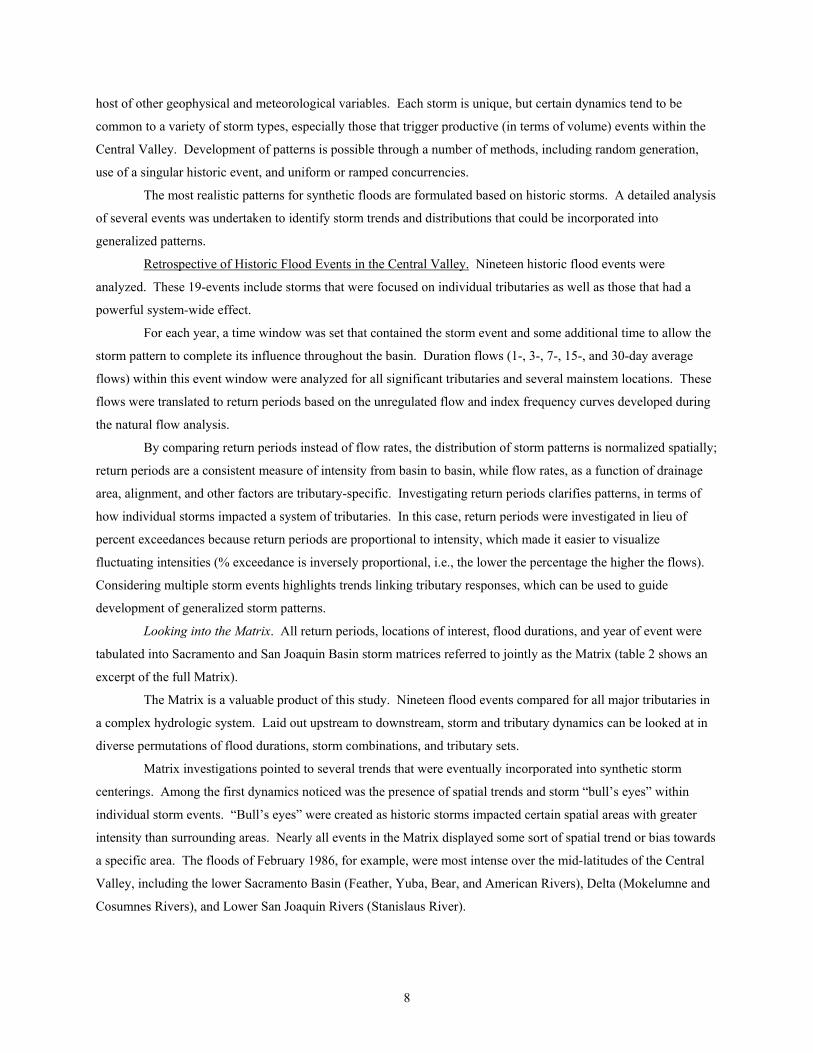
host of other geophysical and meteorological variables. Each storm is unique, but certain dynamics tend to be

common to a variety of storm types, especially those that trigger productive (in terms of volume) events within the

Central Valley. Development of patterns is possible through a number of methods, including random generation,

use of a singular historic event, and uniform or ramped concurrencies.

The most realistic patterns for synthetic floods are formulated based on historic storms. A detailed analysis

of several events was undertaken to identify storm trends and distributions that could be incorporated into

generalized patterns.

Retrospective of Historic Flood Events in the Central Valley. Nineteen historic flood events were

analyzed. These 19-events include storms that were focused on individual tributaries as well as those that had a

powerful system-wide effect.

For each year, a time window was set that contained the storm event and some additional time to allow the

storm pattern to complete its influence throughout the basin. Duration flows (1-, 3-, 7-, 15-, and 30-day average

flows) within this event window were analyzed for all significant tributaries and several mainstem locations. These

flows were translated to return periods based on the unregulated flow and index frequency curves developed during

the natural flow analysis.

By comparing return periods instead of flow rates, the distribution of storm patterns is normalized spatially;

return periods are a consistent measure of intensity from basin to basin, while flow rates, as a function of drainage

area, alignment, and other factors are tributary-specific. Investigating return periods clarifies patterns, in terms of

how individual storms impacted a system of tributaries. In this case, return periods were investigated in lieu of

percent exceedances because return periods are proportional to intensity, which made it easier to visualize

fluctuating intensities (% exceedance is inversely proportional, i.e., the lower the percentage the higher the flows).

Considering multiple storm events highlights trends linking tributary responses, which can be used to guide

development of generalized storm patterns.

Looking into the Matrix. All return periods, locations of interest, flood durations, and year of event were

tabulated into Sacramento and San Joaquin Basin storm matrices referred to jointly as the Matrix (table 2 shows an

excerpt of the full Matrix).

The Matrix is a valuable product of this study. Nineteen flood events compared for all major tributaries in

a complex hydrologic system. Laid out upstream to downstream, storm and tributary dynamics can be looked at in

diverse permutations of flood durations, storm combinations, and tributary sets.

Matrix investigations pointed to several trends that were eventually incorporated into synthetic storm

centerings. Among the first dynamics noticed was the presence of spatial trends and storm “bull’s eyes” within

individual storm events. “Bull’s eyes” were created as historic storms impacted certain spatial areas with greater

intensity than surrounding areas. Nearly all events in the Matrix displayed some sort of spatial trend or bias towards

a specific area. The floods of February 1986, for example, were most intense over the mid-latitudes of the Central

Valley, including the lower Sacramento Basin (Feather, Yuba, Bear, and American Rivers), Delta (Mokelumne and

Cosumnes Rivers), and Lower San Joaquin Rivers (Stanislaus River).

8

Table 2: Excerpt from the Sacramento and San Joaquin River Basins historical flood Matrix (9 of 19 storms analyzed are included). Table contains return periods (in years) for the highest 1-day unimpaired flow during discrete storm event windows. Values do not necessarily reflect the maximum flow experienced in the water year containing the event window. Locations 1-11 are listed north to south in groups of east and westside basins. The storm in 1974 was distinctly northern and not analyzed for San Joaquin River tributaries. Similar tables for the 3-, 7-, 15-, and 30-day durations are available in USACE and Rec Board 2000.

WATER YEAR CONTAINING STORM EVENT WINDOW

ID Location 1997 1995 1986 1983 1982 1974 1967 1956 1951 1 Sacramento River at Shasta 133 6 13 5 2 103 2 18 1 2 Clear Creek near Igo 20 5 4 27 1 40 2 10 1 4 Cottonwood Creek near Cottonwood 8 5 13 20 1 45 1 12 1 3 Cow Creek near Millville 4 2 10 7 1 14 1 2 1 5 Battle Creek below Coleman Fish Hatchery 100 5 9 8 3 48 1 4 1

M1 Sac River at Bend Bridge 67 5 13 12 1 69 1 15 1 6 Mill Creek near Los Molinos 88 5 16 4 3 12 2 9 1 9 Deer Creek near Vina 174 7 23 7 5 10 1 13 1 10 Big Chico Creek near Chico 140 21 19 5 6 4 2 6 1 7 Elder Creek near Paskenta 7 9 14 15 1 14 1 5 1 8 Thomes Creek at Paskenta 5 8 68 3 1 33 1 20 1 11 Stony Creek at Black Butte 9 8 15 10 2 8 1 7 1 M2 Sac River at Ord Ferry (latitude) 40 22 22 13 2 29 2 17 1 12 Butte Creek near Chico >100 5 26 4 5 4 2 16 2 13 Feather River at Oroville 105 10 33 3 5 4 1 20 3 14 North Yuba River at New Bullards Bar 55 4 35 2 5 3 1 37 5 17 Bear River near Wheatland 31 4 74 2 2 2 2 9 5 M3 Sac River at Verona (latitude) 87 8 57 6 4 8 2 40 3 18 Cache Creek at Clear Lake 73 7 14 10 3 5 1 10 1 20 American River at Fair Oaks 78 5 29 2 5 3 1 37 16 M4 Sac River at Sacramento (latitude) 95 8 66 5 4 7 2 38 4 22 Cosumnes River at Michigan Bar 210 7 31 7 4 1 24 6 23 Mokelumne River at Camanche 152 6 18 5 15 2 27 22 25 Calaveras River near New Hogan 10 4 27 4 4 2 4 2 27 Littlejohn Creek at Farmington 7 3 12 4 2 2 9 M5 SJR River at Vernalis (latitude) 89 13 35 6 12 4 58 25 28 Stanislaus River at New Melones 54 8 19 3 11 3 68 35 M6 SJR River at Maze Road Bridge (latitude) 89 16 32 7 13 4 54 19 29 Dry Creek near Modesto 6 16 6 3 12 2 81 1 30 Tuolumne River at Don Pedro 83 10 12 4 12 5 79 20 32 Orestimba Creek near Newman 5 14 8 7 4 2 9 2 M7 SJR River at Newman (latitude) 38 14 23 8 11 5 51 13 33 Merced River at Exchequer 49 15 11 5 16 4 63 22 36 Bear Creek at Bear 6 6 3 5 3 3 36 4 M8 SJR River at El Nido (latitude) 71 19 30 8 19 9 66 10 39 Chowchilla River at Buchanan 12 12 9 8 4 4 182 7 40 Fresno River at Hidden 16 19 10 9 10 6 28 8 41 Big Dry Creek at BDC Dam 10 29 19 7 33 2 19 1 42 San Joaquin River at Friant 61 16 12 4 4 18 57 18 43 Kings River at Pine Flat 34 11 10 3 35 59 76 36

Mainstem locations below these “bull’s eyes” experienced lower return periods, because here the intensity

of flooding is a function of all upstream tributaries, not just those which were especially intense. In this sense, the

mainstem acts as a buffer which absorbs and moderates localized extremes because they alone do not add enough

volume to the system to maintain the high return period.

9

A key finding was that orographic effects were most pronounced in the rarest events. The January 1997

floods were the highest on record in the San Joaquin Basin. In this event, as well as 1982, 1967, 1951 and, to a

lesser extent, 1986 and 1956, return periods were consistently more extreme in the higher elevation San Joaquin

basins than in the foothill tributaries. This relationship highlights the effects of the high Sierra mountain range in

the San Joaquin and Tulare Basins.

Orographic effects in the Sacramento Basin were definitely visible, but not as well defined as those in the

San Joaquin. Still, higher basins in the floods of 1974 and 1956, and to a lesser extent in 1997 and 1986, displayed

distinctively more extreme return periods than the lower basins. It is likely that the more pronounced orographic

influence in the southern Central Valley is related to the average ridge crest elevation along the Sierras, which is

generally lower in the Sacramento Basin than in the San Joaquin and Tulare, but this remains uncertain.

The years cited above for both the Sacramento and San Joaquin Basins basically comprise a subset of the

Matrix containing the most severe historical events analyzed in this study. For storms that were generally less

intense, orographic effects were muted at best and basically not visible. Storms tended to become more and more

evenly distributed until any dynamics that could potentially be tied to orographics were just as likely attributed to

random noise.

The Matrix also points out that natural dynamics are highly variable. Storm cells nested within the larger

storm structure are powerful and have the ability to trigger individual tributaries significantly (i.e., the 1986 flood on

the Bear River). Even with the supporting evidence for orographic influence, there are Matrix examples of storms

that demonstrate a consistently opposite bias; in the San Joaquin Basin during the March 1995 floods and in the

Sacramento Basin during the 1983 floods, return periods for foothill tributaries exceeded those of neighboring

higher basins.

Synthetic Storm Centering Development for X% Exceedance Flood Events. Based on trends identified in

the historic storm analysis and in keeping with the concept of the Composite Floodplain, guidelines for centering

development were formulated and synthetic storm centerings were constructed.

In the context of this study, a storm centering is defined simply as a set of percent exceedances assigned to

a set of tributaries. Centerings were developed separately for the Sacramento and San Joaquin Basins. Each

tributary was included in all centerings within its basin.

Two basic types of storm centerings were analyzed (figure 2). The first consists of basin-wide storm events

(mainstem centerings), which are significant on a regional basis and produce large runoff volumes throughout the

system. The second are tributary specific storms (tributary centerings), which generate extremely large floods on

individual rivers, but are not widespread enough to produce the runoff volumes typical of basin-wide events. Due to the differences in storm character, mainstem and tributary centerings needed to be addressed with

separate sets of governing guidelines. There are similarities between rule sets, but in general, approaches are

dissimilar.

Mainstem centerings designed to stress widespread valley areas. Index frequency curves provide the

hypothetical volumes that the basin will produce during X% exceedance flood events. The role of the mainstem

centerings is to distribute these volumes back into the basin, tributary by tributary, in accordance with patterns

10

visible in historic storm events. Once the volume is distributed it will be translated into hydrographs and routed

through reservoir simulation models to produce the X% regulated hydrographs needed to construct floodplains

throughout the system.

Mainstem centerings reflect a generalized storm pattern based on a number of historic events. Through the

incorporation of multiple floods into one characteristic pattern, relationships between tributaries become more stable

and the influences of powerful, but isolated, storm cells are downplayed.

Characteristic patterns were developed for each mainstem location. Where available, historic events that

displayed flood “bull’s eyes” in the watershed above the mainstem location of interest were used to formulate

synthetic patterns. The orographic effects noted in the Matrix analysis were also incorporated, especially for the

rarest X% events. To assure that patterns were developed consistently, guidelines for mainstem pattern construction

were formulated and are presented in table 3.

Tributary centerings designed to stress individual tributary systems. Whereas mainstem centerings were

formulated as spatially distributed events that were productive on a system-wide basis, tributary centerings were

designed to simulate extreme floods on individual rivers generated by storm systems that were not widespread

enough to produce runoff volumes typical of basin-wide events. In this sense, tributary centerings seek to reflect the

powerful and isolated storm cells intentionally downplayed by the mainstem centerings.

Preparation of tributary centerings (table 4) was more straightforward than those for the mainstem, because

in any tributary centering, the % exceedance of the target tributary was set equal to the desired X% exceedance (i.e.,

the 1% centering for the Tuolumne River includes a 1% inflow to Don Pedro Reservoir). All other tributaries

experience a higher % exceedance. Intertributary relationships were defined using patterns visible in the Matrix.

Table 3: Guidelines for preparation of mainstem centerings.

1) All mainstem centerings must be supported by patterns visible in historic storms.

2) Flood volumes produced by a mainstem centering must be roughly equal to the volumes specified by the index frequency curves.

3) The % exceedance of any individual tributary must exceed that of the mainstem centering being developed.

4) Orographic effects are most pronounced in the rarest events. a) Basins higher in elevation experience less frequent

events than low elevation basins for 1%, 0.5%, and 0.2% mainstem centerings.

b) In 4% and 2% events, orographic effects are less pronounced and mainstem centerings begin to reflect a more evenly distributed pattern.

c) In 50% and 10% events, mainstem centerings reflect an evenly distributed pattern.

5) As an individual tributary becomes more distant from the mainstem location of interest, the % exceedance of that tributary is increased. a) This relationship is maintained within the context

of the fourth rule.

Table 4: Guidelines for preparation of tributary centerings. 1) All tributary centerings must be supported by patterns

visible in historic storms.

a) Generic patterns not supported by the historic storm analysis may need to be applied to tributaries which have not been the focal basin in any of the 19 historic events.

2) The % exceedance of the target tributary is always set equal to the desired % exceedance.

3) No other tributary can have a % exceedance as low as that specified for the target tributary.

a) Percent exceedances for adjacent tributaries are increased by the highest rate visible in historic storm patterns. This maximum rate defines the relationship between those tributaries as the target tributary moves further and further away.

b) Tributary % exceedances are increased in this manner until reaching a baseline percentage, which is a function of the target % exceedance, or until the tributary is distant enough from the target tributary to have no possible influence on that tributary’s floodplain, at which point it would be also be increased to the baseline percentage.

11

Construction of flood hydrographs

To this point, the discussion has focused

primarily on flood frequencies, not on flood flows.

The final topic in the Synthetic Hydrology

Methodology is the translation of frequencies to

hourly flood hydrographs for use in reservoir

simulations and hydraulic modeling (USACE and Rec

Board 2000). The translation process (figure 3)

involved 3 steps: 1) obtain the average flood flow

rates from the unregulated frequency curves; 2)

separate these average flows into wave volumes; and

3) distribute volumes into a wave series. This process

was performed only at the tributary locations.

Mainstem flood hydrographs always resulted from the

routed contributions of upstream tributaries.

Volumes distributed into six 5-day waves to obtain flood series.

Trib 1 Trib 2

Trib 3 Trib 4

Tributary-Specific Patterns

Days

Days Days

Days

Natural Flows

1-day3-day7-day15-day30-day

Exceedance Interval (yrs)

10

100

1000

10 50 100 200 500

Percent Chance Exceedance10 2 1 0.5 0.2

Flow

Flow frequency curves developed for each tributary.

X% volumes obtained from curves and split into 5-day slices.

Flood Volumes

Hydrographs from historic flood events used as patterns.

Flow

Flow

Flow

Flow

0 5 0 5

0 5 0 5 Time (days)5 10 15 20 25 30

5-day volume

30-day volume

Flow

X% Synthetic Rain Flood

Q5

Q10

Q15

Q20

Q25

Q30

V5

V10

V15

V20

V25

V30

V5

V10

V15

V20

V25

V30

Averageflows

Totalvolumes

Wavevolumes

Vwaves are volumes accrued as the floodperiod expands and are distributed

into waves in the pattern hydrograph.

- V5

- V10

- V15

- V20

- V25

Translation of frequencies to hourly flood

hydrographs was automated within a spreadsheet. In

fact, the entire process was mechanized to the point

where generation of the 30-day hourly series was

entirely driven by entering the % exceedances of the

tributaries within each centering into the spreadsheet.

Hydrographs were automatically computed and then

copied into text files for entry into the Hydrologic

Engineering Center’s Data Storage System, HEC-

DSS, which is the database used by HEC-5.

Figure 3: Translation of average natural flows (from frequency curves) to synthetic rain flood hydrographs. The 5-day pattern obtained from historic events is repeated to form a 30-day series.

Reservoir System Modeling

HEC-5, a computer program first developed and distributed in 1973, was designed by the Hydrologic

Engineering Center (HEC) to offer guidance in real-time reservoir release decisions and to aid in planning studies

for proposed reservoirs, operation alternatives, and flood space allocation. HEC-5 reservoir models (figure 4) were

developed, calibrated, and used to simulate the 50%, 10%, 4%, 2%, 1%, 0.5%, and 0.2% exceedance flood events

prepared in the Synthetic Hydrology. Reservoir model results were later input to hydraulic models, which

delineated floodplain areas and defined stage-frequency relationships needed to estimate expected annual flood

damage in the lower basins of the Sacramento and San Joaquin drainages.

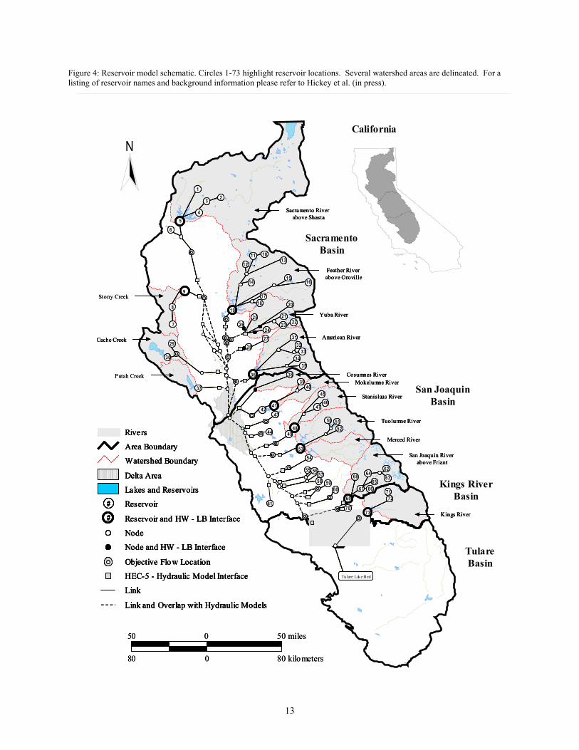
Figure 4: Reservoir model schematic. Circles 1-73 highlight reservoir locations. Several watershed areas are delineated. For a listing of reservoir names and background information please refer to Hickey et al. (in press).

NCalifornia

50 0 50 miles

80 0 80 kilometers

50 0 50 miles

80 0 80 kilometers

Sacramento River above Shasta

Feather River above Oroville

Yuba River

Stony Creek

Cache Creek

Putah Creek

American River

Cosumnes River Mokelumne River

Stanislaus River

Tuolumne River

Merced River

San Joaquin River above Friant

Kings River



Feather River above OrovilleFeather River above Oroville

Yuba River Yuba River

Stony Creek

Cache CreekCache Creek

Putah Creek

American River American River

Cosumnes River Cosumnes River Mokelumne River Mokelumne River

Stanislaus River Stanislaus River

Tuolumne River Tuolumne River

Merced River Merced River



Kings River Kings River

SacramentoBasin

San JoaquinBasin

Kings RiverBasin

TulareBasin

Rivers

Area Boundary

Watershed Boundary

Delta Area


Reservoir

Reservoir and HW - LB Interface

Node

Node and HW - LB Interface

Objective Flow Location

HEC-5 - Hydraulic Model Interface

Link

Link and Overlap with Hydraulic Models

#

#

Rivers

Area Boundary

Watershed Boundary

Delta Area


Reservoir


Node




Link


#

#

Rivers

Area Boundary

Watershed Boundary

Delta Area


Reservoir


Node




Link


#

#

Rivers

Area Boundary

Watershed Boundary

Delta Area


Reservoir


Node




Link


##

##

1

23

40

35

23

4

19

7

10

65

8

1112

13

1615

1718

60

14

9

24

2526

27

20

2122

2829

3937

38

67

3132

333430

36

44

4546

47

66

49

50

68

51

70

4243

41

48 52

71

54

55 5657

58 59

53

61

6263

6465

69 72

73

1

23

40

35

23

4

19

7

10

65

8

1112

13

1615

1718

60

14

9

24

2526

27

20

2122

2829

3937

38

67

3132

333430

36

44

4546

47

66

49

50

68

51

70

4243

41

48 52

71

54

55 5657

58 59

53

61

6263

6465

69 72

73

1

23

40

35

23

4

19

7

10

65

8

1112

13

1615

1718

60

14

9

24

2526

27

20

2122

2829

3937

38

67

3132

333430

36

44

4546

47

66

49

50

68

51

70

4243

41

48 52

71

54

55 5657

58 59

53

61

6263

6465

69 72

73

Tulare Lake BedTulare Lake Bed

13

HEC-5 Methodology

Reservoirs were included based on two criteria: 1) existing flood damage reduction function or 2) active

storage greater than 10,000 ac-ft and regulation of a significant natural drainage area. Most facilities modeled do

not have formal flood damage reduction responsibilities, but all reservoirs alter the form and timing of flood

hydrographs. The influence of non-flood damage reduction reservoirs is significant and cannot be ignored in a

holistic watershed study.

Simulation models were developed for both the Sacramento and San Joaquin River Basins. Due to basin

operations and the number of facilities and control points, these models were further split into headwater models and

lower basin models. The headwater model for each basin generally contains reservoirs located upstream of flood

damage reduction projects. Lower basin models contain those flood projects as well as a few water supply,

recreation, and hydropower facilities.

A 3-step process was required to analyze each storm centering. First, headwaters models were simulated.

Second, using the resulting storage time series for select headwater facilities, top of conservation storage for those

flood damage reduction projects with established credit space agreements were computed. Finally, using results of

the headwaters simulations and computed top of conservation series, the lower basin models were simulated. Full

basin simulations were run for each centering regardless of storm location or intensity.

Headwaters (Step 1)

Headwater reservoirs are typically located in the watersheds above flood damage reduction projects.

Primarily used for water supply and hydropower generation, these facilities do not have formal (Congressionally

authorized) flood operations. A total of 46 headwater reservoirs were modeled, mostly in the Sacramento Basin (28

sites).

Operational Criteria and Physical Characteristics. Headwater reservoirs typically do not have scripted or

published criteria to guide modelers. In this study, criteria were developed through conference calls with facility

owners and operators and analysis of gage data. Elevation-capacity tables, outlet and spillway ratings, and facility

schematics were obtained from the California State Division of Safety of Dams.

Preparing model input. Prior to simulation of headwater reservoirs, flows needed to be split from the single

unregulated flow series at the hydrograph location (prepared in the Synthetic Hydrology) into inflows at all

upstream reservoirs (figure 5). These flow splits were performed for each tributary by multiplying the full

unregulated hydrograph by a constant percentage based on drainage area ratios, normal annual precipitation (NAP)

distribution within the tributary basin, and volume comparisons of historical flood volume yields at the headwater

reservoir and at the full unregulated flow location. In some instances, the volume comparison was not possible due

to a lack of data and the ratio was based solely on NAP distribution and drainage areas.

14

Simulation product. Regulated flows at model interfaces (between headwater and lower basin models)

continue in the simulation process as inflow data for the lower basin simulation models. Comparison of these

computed regulated flows and their corresponding unregulated flows provides an excellent visual of the combined

influence of headwater reservoirs for individual watersheds. These relationships are discussed for the Sacramento

(at Shasta), American, Tuolumne, and San Joaquin (at Friant) Rivers in the results section of this paper.

Top of Conservation Storage (Step 2)

The required top of conservation storage is specified on the

flood control diagram for each project. Typically, the top of

conservation varies seasonally, as a function of basin wetness, and in

some cases as a function of the concurrent storage of reservoirs

upstream of the project.

To Valley

Lower basin reservoirand location of

full basin hydrograph

Headwaters reservoirs

Q in

Q out

12%

10% 8%

65%

Watershedboundary

5%

Percent splits

The basin wetness parameter is a function of the total

precipitation that has fallen over the watershed above the flood

damage reduction reservoir in the rainy season to date. Since the

reservoir models were prepared to simulate flood events and most

major runoff events occur in wet years, computation of the top of

conservation assumed that the basin wetness parameter would be high

enough to reduce the top of conservation to the minimum level in all

X% floods studied. Any seasonal variations along this minimum were

included in the model script.

Top of conservation for projects with established credit

space scenarios (where part of the required flood space in a flood

damage reduction reservoir may be offset by space available at

upstream reservoirs) were computed as an interim process

between simulations of the headwater and lower basin models.

Figure 5: Splitting of a full unregulated hydrograph (generated in the Synthetic Hydrology) into inflows for headwater reservoirs.

Lower Basins (Step 3)

Twenty-four of the 27 lower basin reservoirs have storage dedicated to flood damage reduction. Eighteen

of these reservoirs, all with flood storage, are located in the San Joaquin and Tulare Basins.

In accordance with the Flood Control Act, the USACE has established flood damage reduction operations

for all reservoirs with flood space. These operations are described in Sacramento District-maintained Water Control

Manuals and were incorporated into the models as directly as possible.

Model development focused on flood simulations where flood damage reduction reservoirs are encroached.

15

Physical Characteristics, Objective Flows, and Starting Storage. All required data (elevation-capacity

tables, outlet and spillway ratings, facility schematics, and objective flows) were available in the Water Control

Manuals. Starting storages were set at the top of conservation for all flood damage reduction projects. Reservoirs

are operated to maintain flows at or below objective limits and will (if possible) curtail releases to accommodate

tributary flows confluencing between the dam and the downstream locations.

River Routings. Muskingum routings, procedures which delay and attenuate flows as hydrographs travel

downstream, were used for all river reaches in the lower basin models.

Local Flows. Local flows are unregulated tributaries that join with larger tributaries between reservoirs in

series, between a flood damage reduction reservoir and its objective flow location, or downstream of objective flow

locations. In this study, local flows were modeled in one of two ways. Hydrographs for local flows were either

produced in the Synthetic Hydrology or were computed as a percentage of a nearby natural hydrograph.

Percentages were estimated based on comparisons of short duration maxima (peak, 1-, and 3-day) for the local and

nearby natural hydrographs. These local flows were input into the HEC-5 model and, in some cases, influenced

reservoir outflows by filling part or all of the downstream allowable flows.

ESRD Simulation. Emergency Spillway Release Diagrams are formulated for reservoirs with gated

spillways. Diagram operations trigger only in dire situations and may call for emergency releases above

downstream limits before available flood and surcharge storage is exhausted. Each reservoir’s ESRD is unique.

Some base emergency releases on the rate the pool is rising, others as a function of the inflow. Diagrams often have

ranges of pool elevations that specify the use of different sets of release criteria.

In this study, gated releases were modeled by entering certain characteristics directly (spillway width and

pool elevations for spillway crest and surcharge levels) and adjusting the recession variable (allows HEC-5 to

anticipate the total volume contained in a flood wave and compute releases to best pass that volume) until model

results reflected ESRD operations as closely as possible.

Simulation Product. The lower basin simulation is the final step in translating X% unregulated

hydrographs, produced in the Synthetic Hydrology, to regulated X% flows. In the Comprehensive Study modeling

procedure, these results provide the hydrologic input for hydraulic models, which perform detailed routing of the

flows through foothill and valley floor areas to delineate floodplains and generate stage-frequency information

needed by economic modelers to estimate expected annual damages.

Model Calibration and Verification

Model calibration and verification was unique because the goal was not to reflect recorded history. Instead,

modeling sought to portray “by the book” operations. As severe floods dictate event-specific operations, an ideal

16

validation data set does not exist. Therefore, modelers inspected simulation results to confirm agreement with

operations under existing conditions for headwater and lower basin reservoirs.

Results and Discussion

This section consists of a series of short discussions detailing simulation results of 2 major tributaries in the

Central Valley. Figures 6 and 7 plot sample flood simulations. Results for all tributaries are available in USACE

and Rec Board (2000).

Figure 6: Simulation results for Don Pedro Reservoir (Tuolumne River tributary centering, 2% event).

Figure 7: Simulation results for Friant Reservoir (San Joaquin River at Friant tributary centering, 2% event)

Gross Pool 641.9 106 m3

(520,500 ac-ft)

Top of Conservation

Storage

Top of Conservation

Storage

0 5 10 15 20 25 30Time (Days)

888.0(720)

740.0(600)

592.0(480)

444.0(360)

296.0(240)

148.0(120)

0

6,795(240)

5,663(200)

4,530(160)

3,398(120)

2,265(80)

1,133(40)

0

STOR

AGE

106

m3(1,

000 a

c-ft)

FLOW

m3 /s

(1,00

0 cfs)

Headwater CaptureFriant StorageHeadwater CaptureFriant Storage

Unregulated InflowRegulated InflowRegulated Outflow


Gross Pool 2,503.6 106 m3

(2,030,000 ac-ft)

Top of Conservation

Storage

Top of Conservation

Storage

0 5 10 15 20 25 30Time (Days)

2,959.0(2,400)

2,466.6(2,000)

1,973.3(1,600)

1,480.0(1,200)

986.6(800)

493.3(400)

0

8,494(300)

7,078(250)

5,663(200)

4,247(150)

2,831(100)

1,416(50)

0

STOR

AGE

106

m3(1,

000 a

c-ft)

FLOW

m3 /s

(1,00

0 cfs)Headwater Capture

Don Pedro StorageHeadwater CaptureDon Pedro Storage



Note: Headwater capture is the combined storage in excess of starting storage for headwater reservoirs in the San Joaquin River Basin (above Friant) and is plotted on top of the Friant storage time series.

Tuolumne River

Headwaters. The 3 headwater reservoirs modeled above Don Pedro Reservoir are an important source of

water for the City of San Francisco and are operated first for water supply and then for hydropower. Their

combined gross pool storage is 630,000 ac-ft, of which 160,000 ac-ft is vacant at the start of the model simulations.

These reservoirs regulate 40 percent of the Tuolumne natural inflow to Don Pedro. The combined effects

of these reservoirs reduced the peak inflow by an average of 23.9 percent and captured an average of 80,000 ac-ft

during the critical 4%, 2%, and 1% simulations.

17

Lower Basin. Don Pedro Reservoir has 340,000 ac-ft of flood space and provides flood protection to

downstream areas including the City of Modesto. At Modesto, Dry Creek, a local flow, joins the Tuolumne River.

Don Pedro operates to maintain flows below the Dry Creek confluence within objective limits. Dry Creek’s

influence is visible in Don Pedro simulations when regulated outflows lower while storage and inflow are increasing

(figure 6). Simulation results indicated that Don Pedro will spill in all events more severe than the 4% flood.

San Joaquin River (at Friant)

Headwaters. The Upper San Joaquin is among the most heavily regulated basins within the study area.

Seven headwater reservoirs, which regulate 75 percent of the natural flow at Friant, were included in the model.

Their combined gross pool storage is 590,000 ac-ft, of which 310,000 ac-ft is vacant at the start of model

simulations.

The combination of number of facilities, available storage, methods of operation, spatial distribution, and

percentage of natural flow regulated proved to be very influential in reshaping natural flood hydrographs at Friant.

In fact, the hydrology in the Upper San Joaquin was more altered than that of any other headwater basin. Peak

inflows were reduced by an average of 51.3 percent for all events and approximately 123,000 ac-ft was captured

during the critical 4%, 2%, and 1% simulations.

Lower Basin. Friant Dam has 170,000 ac-ft of flood space. Friant operates for downstream locations

below the Little Dry Creek confluence and at Mendota. Simulations perform very well for criteria below Little Dry

Creek. This accuracy is not apparent for the Mendota location, which is located further downstream, below a large

diversion and a confluence with another significant tributary. Like Don Pedro, simulation results indicated that

Friant will spill in all events more severe than the 4% flood (figure 7).

Conclusions

To define baseline hydrologic conditions for the 50%, 10%, 4%, 2%, 1%, 0.5%, and 0.2% exceedance

flood events, 23 storm centerings were developed. Hydrologic analyses performed for large spatial areas present

challenges and opportunities unique to such ambitious studies. The Comprehensive Study has made possible a

system-wide update for Central Valley unregulated rain flood hydrology and an overall modernization of the models

used by Sacramento District hydrologists and engineers. These accomplishments will prove valuable to the

Comprehensive Study and to future studies undertaken by public and private organizations.

The 73 reservoirs included in the model contain 25,600,000 ac-ft of storage at gross pool. The combined

storage of all Central Valley reservoirs larger than 10,000 ac-ft is 26,100,000 ac-ft (not including the San Luis

Reservoir Complex or facilities outside the study area). Therefore, 98 percent of all gross pool storage in the study

area (in reservoirs larger than 10,000 ac-ft) is simulated with each full model run. To the knowledge of the authors

18

and of the Hydrologic Engineering Center, this report details the largest HEC-5 flood simulation model ever

constructed.

Results of this study provide a good representation of without-project conditions and the models created

will be valuable to further analysis of flood damage reduction alternatives in the Central Valley. Several

conclusions follow:

• Large-scale watershed perspectives improve the overall quality of flood frequency analyses. Linking individual

tributaries and system effects creates inherent checks and balances that can be used by engineers and

hydrologists as quality management criteria.

• Use of generalized storms to simulate high water conditions in mainstem areas is very important to the

consistent incorporation of hydrologic results into hydraulic and economic investigations. In many cases,

violation of the storm centering guidelines would force hydraulic modelers into difficult and subjective

decisions on how to delineate floodplain extent. Working within the “Composite Floodplain” framework

prevents inconsistencies that would complicate ensuing analyses common to both planning studies and

floodplain mapping.

• There seems to be a new emphasis in Congressional appropriations that favors large-scale watershed studies

like the Sacramento and San Joaquin River Basins Comprehensive, the Upper Mississippi River Study, and the

Central and South Florida (Everglades) Project. When studies such as these involve macroscale hydrologic and

hydraulic analyses, the public would be better served if both the USACE and FEMA could utilize the technical

products.

In the past, USACE and FEMA procedures for planning studies and regulatory floodplains have differed.

Ultimately, project goals and stakeholder requirements will diverge sufficiently to prevent a single work from

fulfilling the needs of both, but there is enough overlap in the early (and often most costly) phases to warrant

coordinated technical development. To the authors’ knowledge, procedures documented in this manuscript are

viable for hydrologic support of both regulatory floodplains and flood damage reduction studies. Perhaps

Comprehensive Study concepts can fuel discussion regarding common methodologies.

• Modeling within the “Composite Floodplain” framework for hydrologic and hydraulic studies was elegant.

Storm centerings provided an inherent archival system for model results and, since full basin simulations were

run for each centering regardless of storm location or intensity, model adjustments between simulations were

trivial. In fact, only the names of the input data needed to be changed when assessing a different storm

centering.

• After viewing the multitude of Comprehensive Study flood simulations, it is difficult not to step back and

consider the awesome regulating influence of reservoirs in California’s Central Valley. In the 2 simulation

19

excerpts presented, peak flows were reduced by an average of 78 percent. And these were events that exceeded

the flood management capabilities of the tributary systems. Lesser floods simply flat-lined or did not approach

allowable release limits.

As society has developed around this protection, it is difficult to foresee a future where the roles of

reservoirs in flood damage reduction are greatly reduced. Instead, operations will need to deal with an

increasing variety of demands, especially in the environmental arena where prescribed variability (i.e.,

experimental and, eventually, designed flooding) will one day become accepted operations for reservoirs

controlling long downstream reaches with ecosystems that bear or could bear semblance to natural conditions.

• To date, this work has been well received by technical reviewers, public and private agencies, and the general

public. Credibility has been enhanced through the exhaustive use of available historic data and by operating

within the context of standard frequency analysis guidelines. These have been key to the ongoing acceptance of

this large, high profile study.

Products of the hydrology and reservoir efforts feed ongoing hydraulic, economic, and ecosystem modeling.

From supporting emergency operations with real-time modeling of river flows, floodplains, and damages, to the

scientific study of controlled flooding designed to reestablish riparian habitats, the potential of this group of linked

models is tremendous.

References

Hickey, J. T., Bond, M. V., Patton, T. K., Richardson, K. A., and Pugner, P. E. (In Press). “Reservoir Simulations of Synthetic Rain Floods for the Sacramento and San Joaquin River Basins.” Journal of Water Resources Planning and Management. Hickey, J. T., Collins, R. F., High, J. M., Richardson, K. A., White, L. L., and Pugner, P. E. (2002). “Synthetic rain flood hydrology for the Sacramento and San Joaquin River Basins.” Journal of Hydrologic Engineering, 7, 195-208. Hydrologic Subcommittee. (1981). “Guidelines for determining flood flow frequency.” Bulletin 17b, Interagency Advisory Committee on Water Data, U.S. Geological Survey, U.S. Department of the Interior, Reston, Virginia. U.S. Army Corps of Engineers (USACE). (1972). “Regional frequency computations.” Hydrologic Engineering Center, Davis, Calif. U.S. Army Corps of Engineers (USACE). (1992). “HEC-FFA: Flood Frequency Analysis user’s manual.” Hydrologic Engineering Center, Davis, Calif. U.S. Army Corps of Engineers (USACE). (1998). “HEC-5: Simulation of flood control and conservation systems.” Hydrologic Engineering Center, Davis, Calif. U.S. Army Corps of Engineers (USACE), and The Reclamation Board, State of California (Rec Board). (1999). “Post-flood assessment.” Sacramento and San Joaquin River Basins Comprehensive Study, Sacramento, Calif. U.S. Army Corps of Engineers (USACE), and The Reclamation Board, State of California (Rec Board). (2000). “In progress review document.” Sacramento and San Joaquin River Basins Comprehensive Study, Sacramento, Calif. U.S. Congress, House of Representatives, Committee on Appropriations, (1998). “Energy and water development appropriations bill, 1998.” House Committee Report 105-190. Washington, D.C.

20

Documents

Hypothetical Hydrology for the Sacramento and San Joaquin Valleys