Embed Size (px)
Citation preview

Hyperspectral Imaging for Diffuse Optical Tomography
Thesis
submitted by
Friðrik Lárusson, M.S.
In partial fulfillment of the requirementsfor the degree of
Master of Science
in
Electrical and Computer Engineering
TUFTS UNIVERSITY
September 2009
ADVISER: Prof. Eric L. Miller

Copyright
by
Friðrik Lárusson
2009

Dedication
To my parents. They have taught me everything that I know about being a
respectable person and a researcher. And more.

Acknowledgments
I would like to thank Professor Eric Miller for his assistance and advice as my thesis
advisor. He always made time to help me with this thesis and is always successful
in showing me the right path.
I am very grateful to Professor Sergio Fantini for all his help on his thesis
and for letting me into his lab to meet his great students.
To Professor Angelo Sassaroli, Debbie Chen, Ning Li and Yang Yu on all
those discussions and helpful pointers on the experimental side of things. Without
them the experimental process would have taken much longer.
To my brother for always keeping me up to date on my programming, orga-
nizing and regular peptalks.
To Nicholas Rotker and Ashwin Duggal for making my transition to the USA
and graduate school a very easy one.
Finally, I would like to thank my committee of Professor Eric Miller, Professor
Sergio Fantini and Professor Misha Kilmer, for taking the time to review this thesis.
iv

Abstract
Diffuse optical tomography (DOT) has emerged in the last decade as a new and
exciting tool for functional medical imaging with applications in a range of areas
including breast cancer detection and diagnosis. DOT employs observations of near
infrared (NIR) light that has propagated through tissue to reconstruct the spatial
distribution of various chromophores present in the region of interest. In the case of
breast cancer, oxygenated and de-oxygenated hemoglobin are of particular interest in
identifying and characterizing tumors. It is well known that the DOT reconstruction
process can be quite sensitive to noise and other un-modeled effects due to the
diffusive nature of the underlying physics as well as the limited aperture over which
data can be acquired in many practical systems. While there exist a wide array of
mathematical techniques for stabilizing the reconstruction, ideally one would like a
richer data set. Most DOT instruments employ no more than five NIR wavelengths
to probe the tissue; however recent work in the diffuse optical imaging group in
the Biomedical department has led to the development of a hyperspectral system in
which hundreds of wavelengths can be acquired. With the increase in data however
comes an associated rise in the complexity of the image formation process. In this
thesis, we explore the development and performance of algorithms for hyperspectral
DOT. We detail an efficient method for forming the images based on the use of
iterative algorithms applied to a linearized measurement model. Simulation and
experimental results will be provided which show the advantages of hyperspectral
imaging.

Contents
Acknowledgments iv
List of Tables iv
List of Figures v
Chapter 1 Introduction 1
Chapter 2 Diffuse Optical Tomography 7
2.1 Early Development . . . . . . . . . . . . . . . . . . . . . . . . . . . . 7
2.1.1 Pulse oximetry . . . . . . . . . . . . . . . . . . . . . . . . . . 8
2.1.2 Doppler Blood-Flowmetry . . . . . . . . . . . . . . . . . . . . 9
2.1.3 NIRS . . . . . . . . . . . . . . . . . . . . . . . . . . . . . . . 9
2.2 Application of DOT . . . . . . . . . . . . . . . . . . . . . . . . . . . 11
2.2.1 Breast Imaging . . . . . . . . . . . . . . . . . . . . . . . . . . 11
2.2.2 Optical Based Brain Imaging . . . . . . . . . . . . . . . . . . 22
2.2.3 Optical Based Joint Imaging . . . . . . . . . . . . . . . . . . 24
2.2.4 Fluorescence Imaging . . . . . . . . . . . . . . . . . . . . . . 25
2.2.5 Hyperspectral and Multispectral . . . . . . . . . . . . . . . . 26
2.3 DOT forward model . . . . . . . . . . . . . . . . . . . . . . . . . . . 28
i

2.3.1 Discrete model and use of Green’s function . . . . . . . . . . 28
2.3.2 Born Approximation . . . . . . . . . . . . . . . . . . . . . . . 29
2.3.3 3D computation . . . . . . . . . . . . . . . . . . . . . . . . . 34
Chapter 3 The Inverse problem 37
3.1 Inversion Methods . . . . . . . . . . . . . . . . . . . . . . . . . . . . 37
3.1.1 SVD and TSVD methods . . . . . . . . . . . . . . . . . . . . 37
3.1.2 Iterative Methods . . . . . . . . . . . . . . . . . . . . . . . . . 40
3.1.3 Computational issues . . . . . . . . . . . . . . . . . . . . . . . 44
Chapter 4 Simulations 47
4.1 Simulated Images . . . . . . . . . . . . . . . . . . . . . . . . . . . . . 48
4.2 Using gradient matrix and two parameters . . . . . . . . . . . . . . . 52
4.3 Reconstruction . . . . . . . . . . . . . . . . . . . . . . . . . . . . . . 54
4.3.1 First set . . . . . . . . . . . . . . . . . . . . . . . . . . . . . . 55
4.3.2 Second set . . . . . . . . . . . . . . . . . . . . . . . . . . . . . 56
4.3.3 Third set . . . . . . . . . . . . . . . . . . . . . . . . . . . . . 58
Chapter 5 Physical Measurements 63
5.1 Measurement Process . . . . . . . . . . . . . . . . . . . . . . . . . . . 63
5.1.1 Phantoms . . . . . . . . . . . . . . . . . . . . . . . . . . . . . 64
5.1.2 Background . . . . . . . . . . . . . . . . . . . . . . . . . . . . 65
5.1.3 Spectrograph . . . . . . . . . . . . . . . . . . . . . . . . . . . 67
5.2 Results . . . . . . . . . . . . . . . . . . . . . . . . . . . . . . . . . . . 69
5.2.1 First set . . . . . . . . . . . . . . . . . . . . . . . . . . . . . . 70
5.2.2 Second set . . . . . . . . . . . . . . . . . . . . . . . . . . . . . 74
ii

Chapter 6 Conclusion 82
Bibliography 84
iii

List of Tables
5.1 Concentrations of the phantoms used in measurements. The medium
was made out of 2 parts water and 1 part milk. . . . . . . . . . . . . 64
5.2 Value of μa from measurements compared to the value used from
literature. . . . . . . . . . . . . . . . . . . . . . . . . . . . . . . . . . 66
iv

List of Figures
1.1 The process of photons passing through tissue [BBM+01]. . . . . . . . . . 4
2.1 An example of the "banana path" encountered in Ultrasound imaging [ZTK07]. 19
2.2 Different z-planes along the z axis. . . . . . . . . . . . . . . . . . . . . . 35
4.1 Molar extinction coefficents used in simulations plotted as a function
of wavelength. . . . . . . . . . . . . . . . . . . . . . . . . . . . . . . . 49
4.2 Simple concentration images for a single chromophore. Left image is
for HbO2 and right image is for HbR. . . . . . . . . . . . . . . . . . . 50
4.3 Images with concentrations for two chromophores. Left image is for
HbO2 and right image is for HbR. . . . . . . . . . . . . . . . . . . . . 50
4.4 Images with concentrations for two chromophores with different inten-
sities. Left image is for HbO2 and right image is for HbR. . . . . . . 50
4.5 The setup of sources and detectors. . . . . . . . . . . . . . . . . . . . . . 51
4.6 Mean square error as function of regularization parameters for the
first set. Left image is HbO2 and right image is HbR. . . . . . . . . . 54
4.7 Mean square error as function of regularization parameters for the
second set. Left image is HbO2 and right image is HbR. . . . . . . . 54
v

4.8 Reconstruction for first set, low complexity. Middle images is done
with 6 wavelengths and rightmost images is done with 26 wavelengths.
Upper row is for the HbO2 chromophore and the lower for HbR. SNR
is 64.9 dB. . . . . . . . . . . . . . . . . . . . . . . . . . . . . . . . . . 57
4.9 Reconstruction for first set, low complexity. Middle images is done
with 126 wavelengths and rightmost images is done with 251 wave-
lengths. Upper row is for the HbO2 chromophore and the lower for
HbR. SNR is 63.9 dB. . . . . . . . . . . . . . . . . . . . . . . . . . . 57
4.10 MSE plotted as a function of the number of wavelengths for the first set. 58
4.11 Symmetric difference plotted as a function of the number of wave-
lengths for the first set. . . . . . . . . . . . . . . . . . . . . . . . . . . 58
4.12 Reconstruction for second set, medium complexity. Middle images is
done with 6 wavelengths and rightmost images is done with 26 wave-
lengths. Upper row is for the HbO2 chromophore and the lower for
HbR. SNR is 83.6 dB. . . . . . . . . . . . . . . . . . . . . . . . . . . 59
4.13 Reconstruction for second set, medium complexity. Middle images is
done with 126 wavelengths and rightmost images is done with 251
wavelengths. Upper row is for the HbO2 chromophore and the lower
for HbR. SNR is 90.6 dB. . . . . . . . . . . . . . . . . . . . . . . . . 59
4.14 MSE plotted as a function of the number of wavelengths for the second
set. . . . . . . . . . . . . . . . . . . . . . . . . . . . . . . . . . . . . . 60
4.15 Symmetric difference plotted as a function of the number of wave-
lengths for the second set. . . . . . . . . . . . . . . . . . . . . . . . . 60
vi

4.16 Reconstruction for third set, high complexity. Middle images is done
with 6 wavelengths and rightmost images is done with 26 wavelengths.
Upper row is for the HbO2 chromophore and the lower for HbR. SNR
is 80.7 dB. . . . . . . . . . . . . . . . . . . . . . . . . . . . . . . . . . 61
4.17 Reconstruction for third set, high complexity. Middle images is done
with 126 wavelengths and rightmost images is done with 251 wave-
lengths. Upper row is for the HbO2 chromophore and the lower for
HbR. SNR is 85.5 dB . . . . . . . . . . . . . . . . . . . . . . . . . . . 61
4.18 MSE plotted as a function of the number of wavelengths for the third
set. . . . . . . . . . . . . . . . . . . . . . . . . . . . . . . . . . . . . . 62
4.19 Symmetric difference plotted as a function of the number of wave-
lengths for the third set. . . . . . . . . . . . . . . . . . . . . . . . . . 62
5.1 (a) Absorption spectra for set #1.(b)Absorption spectra for set #2. . 65
5.2 Target image for the first measurement taken on January 28th 2009.
This is using only a single ink phantom from set #2. Upper image is
for ink and lower image is for dye. . . . . . . . . . . . . . . . . . . . 68
5.3 Target image for the first measurement taken on May 28th 2009. Both
ink and dye phantoms from set #2 were used. Upper image is for ink
and lower image is for dye. . . . . . . . . . . . . . . . . . . . . . . . 69
5.4 Reconstruction done for a single ink phantom. 3 wavelengths and 21
z-planes used. Upper image is for ink and lower image is for dye. . . 71
5.5 Reconstruction done for a single ink phantom. 6 wavelengths and 21
z-planes used. Upper image is for ink and lower image is for dye. . . 71
5.6 Reconstruction done for a single ink phantom. 13 wavelengths and 21
z-planes used. Upper image is for ink and lower image is for dye. . . 72
vii

5.7 Reconstruction done for a single ink phantom. 26 wavelengths and 21
z-planes used. Upper image is for ink and lower image is for dye. . . 72
5.8 MSE displayed for second measurement set for ink at every wavelength. 73
5.9 The symmetrical difference of reconstructions for the first set plotted
as a function wavelength. . . . . . . . . . . . . . . . . . . . . . . . . 74
5.10 Localization of reconstruction of the ink for the first set plotted with
respect to the target image. . . . . . . . . . . . . . . . . . . . . . . . . 74
5.11 Reconstruction done for two ink and dye phantoms. 3 wavelengths
and 21 z-planes used. Upper image is for ink and lower image is for
dye. . . . . . . . . . . . . . . . . . . . . . . . . . . . . . . . . . . . . 76
5.12 Reconstruction done for two ink and dye phantoms. 6 wavelengths
and 21 z-planes used. Upper image is for ink and lower image is for
dye. . . . . . . . . . . . . . . . . . . . . . . . . . . . . . . . . . . . . 77
5.13 Reconstruction done for two ink and dye phantoms. 9 wavelengths
and 21 z-planes used. Upper image is for ink and lower image is for
dye. . . . . . . . . . . . . . . . . . . . . . . . . . . . . . . . . . . . . 77
5.14 Reconstruction done for two ink and dye phantoms. 26 wavelengths
and 21 z-planes used. Upper image is for ink and lower image is for
dye. . . . . . . . . . . . . . . . . . . . . . . . . . . . . . . . . . . . . 78
5.15 Reconstruction done for two ink and dye phantoms. 251 wavelengths
and 21 z-planes used. Upper image is for ink and lower image is for
dye. . . . . . . . . . . . . . . . . . . . . . . . . . . . . . . . . . . . . 78
5.16 MSE displayed for second measurement set for ink and dye at every
wavelength. . . . . . . . . . . . . . . . . . . . . . . . . . . . . . . . . 80
viii

5.17 The symmetrical difference of reconstructions for the second set plotted
as a function wavelength. . . . . . . . . . . . . . . . . . . . . . . . . 80
5.18 Localization of reconstruction for the second set plotted with respect to
the target image. Upper image is for ink and lower image is for dye. 81
ix

Chapter 1
Introduction
In the past 10 years there has been increased research into the use of near-infrared
light to image inside the human body. One of the techniques of interest is diffuse
optical tomography(DOT) [GBD+00]. DOT is sensitive to the functional state of
tissue such as the consumption of oxygen which is relevant to processes such as the
growth of tumors as well as the state of brain activity. Specifically, the DOT method
uses near-infrared light at multiple wavelengths, which allows for reconstruction of
the space and time varying profiles of chromophore concentrations (oxy- and deoxy-
hemoglobin, water and lipids etc.) The latter of which convey functional information
about the body [LBZ+05]. Although many applications have been shown for the
DOT method the most promising ones are for breast imaging or brain imaging
[FHP+05, SA99]. This thesis will focus on breast imaging but discussion on brain
imaging and other applications can be found in Chapter 2.2.
Breast imaging researchers have for a long time been dependent on informa-
tion from 3D imaging modalities, such as X-ray computed tomography (CT) and
magnetic resonance imaging (MRI). Still, there are some drawbacks that plague
1

these imaging methods. MRI remains a large and fairly expensive system and can
entail a considerable maintenance cost. CT on the other hand exposes the patient to
considerable amount of ionizing radiation which can be harmful. Recently the idea
of detecting breast cancer has shifted from anatomical information, obtained from
CT and MRI, and towards functional imaging modalities.
DOT represents a very strong candidate for providing this type of information
specifically in the context of breast imaging. As was mentioned above, DOT uses
near-infrared light, which in essence is electro-magnetic radiation but is at a signifi-
cantly lower energy level than CT. Operating in the infrared spectrum, 650-900nm,
gives us a range which is sometime called the window of transparency [SGA03]. In
this window light propagates relatively far into the tissue(on the order of centime-
ters) before being absorbed thereby allowing us to probe quite deeply. Additionally,
light is also scattered within the tissue where it interacts with subsurface inhomo-
geneities. This process is illustrated in Figure 1.1. Within the window, light is
absorbed and scattered differently at different wavelengths depending on the space-
varying oxygenation state of the tissue. This relation gives us a way to using multiple
wavelengths when estimating chromophore concentrations which is the basis of this
thesis. Using different wavelengths, performing multi- or hyperspectral measure-
ments, more information is added to the system by using more complete spectral
information to improve the ability to determine the concentrations of chromophores.
With this method it is possible to increase the effectiveness and accuracy of the DOT
method.
Light propagating through tissue is highly scattered but significant advances
have been made in recent years to solve the problem efficiently, both in terms of theo-
retically modeling the physics and developing useful codes for simulating the process
2

and thereby setting the DOT method up as the prime candidate for future breast
cancer detection systems. X-ray radiation in CT travels generally in a straight line,
excluding Compton and Rayleigh scattering, resulting in a much simpler problem
than DOT. In the case of diffuse optical tomography the photon’s mean free path
of travel between two scattering events is very short, most often only a fraction of a
millimeter. Because of this, any photon traveling through a human breast undergoes
numerous scattering events. Thus, unlike CT where the physics of the problem is
basically straight line propagation and yields a linear relationship between the quan-
tity of interest tissue density and the observed data, for DOT a far more complex
model is required [SGA03]. More specifically, the physics of light interaction with
the tissue is well modeled using a diffusion equation and, as we discuss in Section 2.3,
yield a complicated, nonlinear relationship between the chromophore concentrations
and the observations of scattered light [SGA03]. This model works well when scat-
tering is stronger than absorption, which is frequently the case for biological tissue
and is certainty justified for the breast imaging problem. Diffuse light propagation
complicates the image reconstruction, an efficient way to model the propagation is
to use the diffusion equation as the model. The diffusion equation expresses the
photon density as a function of absorption coefficient and scattering coefficient and
solving it will always provide the forward model needed to solve the inverse problem
[GBD+00, BBM+01].
In the case of DOT, the goal is to estimate the concentrations of different
chromophores based on the measured photons scattering and absorbing in the tissue.
Depending on the wavelength observed by the detectors different scattering and ab-
sorption can be calculated from the measured data. This dependence of wavelength
encourages the use of hyperspectral information.
3

Figure 1.1: The process of photons passing through tissue [BBM+01].
The DOT method is a nonlinear ill-posed inverse scattering problem due to
the physics of the diffusion process just described [BBM+01]. In this thesis, our pri-
mary objective is to explore the utility of hyperspectral data on the DOT problem.
Thus, we simplify the inverse problem by linearizing the physics using a proce-
dure known as the Born approximation [GBD+00]. The ill-posedness poses a more
substantive problem than the non-linearity. Ill-posedness means large changes in pa-
rameters yield fairly small changes in the data. In some sense this is a physics-based
phenomenon, which means there is a lack of sensitivity in the data to the parame-
ters. It also means that in the image formation process(if you do it naively), small
changes in the data from noise and unmodeled effects can cause very large changes
to the estimated profiles. In other words the reconstruction process is highly sen-
sitive to small perturbations in the data. Adding to these difficulties is the fact
that in many cases one seeks to recover more degrees of freedom (voxel values times
number of chromophores) than one has data points [BBM+01]. For the linear prob-
lem we consider, even without noise, the resulting inverse problem has no unique
solution which again is a major problem [LBZ+05, BBM+01]. Taken together, the
4

physics-based ill-posedness coupled with the inherent underdetermined nature of the
problem severely complicates our ability to stably recover useful information about
the state of the tissue from DOT data.
These issues are addressed in two ways. First, regularization techniques are
employed to stabilize the reconstructions. When introducing regularization to the
system, we take advantage of a priori information that we know is true for the phys-
ical system. By choosing the right regularization this a priori information is added
to the system, i.e. the smoothness of the system or that the chromophore concen-
trations are small and slowly changing. Therefore, if we have some information on
the true chromophore concentrations, the regularization can be constructed in such
a way that the solution is drawn towards the known distribution by the regulariza-
tion. The other method used to reduce the ill-posedness is to add information to the
system. In this thesis this is done by using hyperspectral information. By recovering
concentrations using multiple wavelengths we take advantage of as much information
as is available to us. Exploring the advantage of adding data to the system in this
way is the aim of thesis. By employing the fact that near-infrared light scatters and
absorbs depending on wavelengths and the chromophores that it is travelling through
it will be possible to create accurate concentration images for multiple chromophores
simultaneously. Efforts have been made in multispectral DOT imaging, using only
3-5 wavelengths. Here we will examine the effects of including more complete spec-
tral information in the reconstructions. By including hyperspectral data we will use
tens to hundreds of wavelengths in order to deal with the ill-posedness of the DOT
problem. We will also examine how hyperspectral data gives way to distinguishing
between different chromophores. A forward model will be constructed and inversion
techniques will be discussed and employed to solve for chromophore concentrations.
5

In Chapter 2 we review the history and many applications where DOT can
be employed. In that chapter we also define the forward model for the problem. In
Chapter 3 we discuss the inverse problem and what methods are traditionally used
to solve it along with discussing regularization techniques. In Chapters 4 and 5 we
discuss results from simulations and experiments, respectively.
6

Chapter 2
Diffuse Optical Tomography
Throughout history, researchers have devoted significant efforts to the application
of visible and near-infrared light for the detection of breast cancer as well as other
applications. In this chapter we start by reviewing the applications as well as the
early development for DOT, and then move on to introducing the forward model for
the problem.
2.1 Early Development
Research on optical imaging started early as 1920 and a pioneering article from
Max Cutler on optical transillumination images of the breast was released in 1929
[Cut29, LCY+07]. Specifically, light has been used to detect certain information such
as the blood oxygenation level using pulse oximeters since the 1930’s. While this
is not really optical imaging, it illustrates one way where light carries information
about the material through which it travels. Cutler proposed using continuous light
to detect breast lesions but this idea was quickly dropped since the intensity of light
required caused the patient’s skin to overheat. In the 1970’s and the early 1980’s
7

significant developments were made that led to commercially available equipment
for optical mammography. [GQH72] introduced a concept named diaphanography,
in which the breast was positioned between a visible or near-infrared light source
and the physician. From this setup the doctor perceived images using his eyes
alone. These advances led to the development of pulse oximetry, laser Doppler blood-
flowmetry and near infrared spectroscopy(NIRS) which then led to progress in the
areas of continuous-wave time-domain, and frequency domain optical mammography
[LCY+07].
2.1.1 Pulse oximetry
Pulse oximetry was originated in the 1930s and is widely used to monitor patient well
being. Pulse oximeters provide accurate information on arterial blood oxygen satu-
ration. The advantage of optical oximeters over oxygen tension monitors, which need
to be a part of the circulation or have a blood sample, is that they provide a rapid
response to changes in blood oxygenation and yet are non-invasive [BBM+01]. The
first oximeter was an ear oximeter which only used a lamp and a photocell [Pet86].
It measured average hemoglobin oxygen saturation across vascular compartments.
Later it evolved into the more robust pulse oximeter, whose mathematical model is
based on an arterial pulse-triggered measurement of the intensity of the light passing
through the tissue. After each heartbeat the arteries expand, increasing the volume
of blood flowing through them. This causes an increase in the absorption of light
in the tissue and therefore the light attenuated by the blood varies as function of
the pumping of the heart. Comparing the maximum and minimum absorption the
difference can be put into a mathematical model which gives the arterial oxygen
saturation [BBM+01].
8

2.1.2 Doppler Blood-Flowmetry
The invention of the laser quickly gave rise to its use in medical applications. As
early as the 1970s the laser was being used for laser Doppler studies of blood flow
[BBM+01]. When a beam of laser light with uniform intensity is incident on a rough
surface, the reflection of the beam will not be completely uniform but will include
some dark and light spots [TRBS74]. These dark spots, called speckles, are caused
by light reflected many different times which causes interference at the detector.
This is exactly what occurs when light travels though a highly scattering sample.
Additionally, if the scattering particles, red blood cells in the DOT case, are moving
the speckle pattern will fluctuate with a time scale which depends on the motion.
This was the basis for Laser Doppler Blood Flowmetry in the 1960s.
2.1.3 NIRS
Attempts at applying pulse oximetry and laser Doppler blood flowmetry to measure
hemodynamics in the brain were hindered by the photodetector bandwidth limits
and photon limits. In the 1970s NIRS was developed to monitor baseline changes in
total oxygenation in the brain, as revealed by the average intensity of diffusely re-
flected light [CD88, Job77, Cop91]. Briefly, NIRS quantifies changes in chromophore
concentration within highly scattering tissue by measuring the change in the photon
density of light which is diffusely transported through it. The concentration change
of each chromophore is then computed by relating them to the measured change in
photon density. The measured change in photon density is directly related to the con-
centration change by the extinction coefficient of the chromophores and the effective
pathlength of the tissue. The extinction coefficient is an intrinsic property of each
chromophore, but the effective pathlength must be estimated for each measurement
9

as it is heavily dependent upon the measurement setup and the optical properties
of the tissue [BBM+01]. The 1980s brought continuing research into using NIRS
for monitoring cerebral oximetry. It became apparent that the major limitations of
NIRS was it could not measure concentrations of deoxy-hemoglobin and hemoglobin
without calibration of the optical pathlength through tissue. To measure this path
length picosecond pulsed lasers and time-resolved measurements were used in the late
1980s and with that the absorption coefficient and related hemoglobin parameters
could be obtained. Instrumentation and complexity became burdensome and more
expensive, and thus investigators introduced the use of inexpensive and simple radio
frequency modulated laser and measurements of the phase delay of the amplitude
modulated light. This provided a measure of the mean tissue optical pathlength and
subsequently of the hemoglobin parameters.
In the late 1980s and early 1990s it was soon realized that photon migration
spectroscopy measurements could be extended to imaging by solving the inverse
problem as is done with X-Ray computed tomography. Research investigating this
possibility began in the late 1980s and was reviewed by other investigators [Arr93,
BGW+93]. The time domain systems produce illumination by picosecond pulses of
light. This short pulse allows detection of the temporal distribution of photons as
they leave the tissue. The shape obtained from this distribution provides information
about the optical properties of tissue. CW systems emit light at a constant amplitude
or are modulated at a certain frequency. These systems measure the amplitude decay
of the incident light. For frequency domain systems the light is on constantly but is
amplitude-modulated at frequencies on the order of tens to hundreds of megahertz.
This allows the absorption and scattering properties of tissue to be obtained by
recording amplitude decay and phase delay of the detected signal [BBM+01].
10

2.2 Application of DOT
Currently the main applications for diffuse optical tomography are breast, brain,
limb, joint and fluorescence/bioluminescence imaging. As discussed in Chapter 1 the
application investigated in this thesis is the imaging of the breast. To demonstrate
the wide array of possibilities for near-infrared imaging this section will review each
applications in addition to discuss the use of DOT with other modalities in the
context of breast imaging.
2.2.1 Breast Imaging
Research on this topic started very early as mentioned in Section 2.1. After efforts
made in the early 20th century, 1980’s investigators for the breast cancer application,
started using video cameras as detectors and explored methods to use something
other than just the eye as detectors. In 1982 Carlsen published a seminal paper
that included a real-time live viewing but more importantly included spectral in-
formation [BBM+01]. These developments led to a number of pilot clinical studies
later in the decade. Some of these studies reported promising data and projected
a positive attitude about the potential of optical mammography, although some re-
searchers raised questions about its clinical viability [LCY+07]. In the late 1980’s a
multi-center clinical study on a population of 2,658 women concluded that optical
mammography was inferior to standard mammography, obviously showing that sig-
nificant advancements were needed before optical imaging of he breast could play a
clinical role [LCY+07].
Around 1990 a Swedish study found that light scanning was inferior to other
modalities, the probability of actual detection was low and the probability of false
alarm was almost three times higher than in breast imaging methods such as CT or
11

MRI. This caused a significant departure from research concerning optical mammog-
raphy and it was basically abandoned in the early nineties. Some of the factors that
gave rise to optical mammography after this fall were more quantitative approaches
to describing light propagation inside biological tissue together with the development
of time-resolved experimental techniques[LCY+07]. After pulse oximetry, Doppler
blood-flowmetry and NIRS were established, as discussed in Section 2.1, significant
efforts have been made to develop DOT for breast cancer.
When reconstructing images for concentrations of chromophores in DOT
there generally two ways of using spectral information. In this project these two
methods will be referred to as the direct method and the indirect method. The indi-
rect method has three steps to obtain the concentration images. First, measurements
are taken at two or more wavelengths. Second, images of the absorption and reduced
scattering coefficients at the different wavelengths are reconstructed separately and
finally the concentration of the separate hemoglobin are derived from the optical
properties. On the other hand the direct method skips the step of constructing
the spectral absorption images and directly reconstructs the images for hemoglobin
[LZC+04]. For this project we will examine the direct method.
In DOT three measurement schemes are used for measuring the light trans-
mitted through tissue. They are time domain, frequency domain and continuous
wave, which is essentially zero frequency [FFG+96, BBM+01]. For a case like breast
cancer, detection transmission is measured but for a case of brain imaging reflection
is measured [CCD+05]. In some cases measuring both transmission and reflection
could be useful. Out of these schemes the CW method is the simplest, least expen-
sive, and provides the fastest data collection.
The advantage of functional information obtained from DOT is especially
12

encouraging when comparing it to common modalities like X-ray mammography.
Unlike X-ray mammography, which detects microcalcification characteristic of ma-
lignant lesions, optical mammography senses changes in blood perfusion of the tissue
surrounding the tumor. These changes occur early in a tumor’s growth and can affect
a relatively large area [SGA03]. Researchers have developed several instrumentation
types for optical mammography, some are similar to X-ray by compressing the breast
but others use an unconstrained mesh of detectors where sources and detectors are
arranged in planes on the surface [CvdMH+99, LCY+07, ZJ05]. When the compres-
sion technique is used a laser source scans across one plate, which is transparent
while a detector on the opposite plate scans over several measurement locations for
each source position [SGA03]. This arrangement reduces the thickness of the transil-
luminated tissue. This technique has of course been used for several years in X-ray
mammography and has been proven to improve the detectability of deeply embed-
ded objects. One down side of the compression method is that it can cause blood to
drain from the breast, thereby unpredictably altering the optical properties.
The other method, with sources and detectors situated in a plane around an
uncompressed breast, has the patient lying prone on a table with the unsupported
breast suspended in a cavity. The data acquisition might consist of a set of fixed
sources and detectors or a rotating system that scans the breast’s surface. This setup
can provide a more complete sampling data over the boundary, but makes defining
the problem’s geometry more difficult. This also has the advantage that this should
be much more comfortable since numerous patients have felt the compression method
to be uncomfortable and sometimes painful.
Creating a system that makes use of the benefits of DOT with other imaging
modalities could be very useful in the future. To enhance DOT performances, re-
13

searchers have proposed fusing optical techniques with other medical imaging modal-
ities. The high contrast benefits of the DOT method can be used with the high
resolution image of and X-ray or MRI image. The high contrast advantages of us-
ing the DOT method sparks interest to use the DOT method with other imaging
techniques because it offers unique functional information(such as tissue, oxy- and
deoxy-hemoglobin concentrations) while high resolution anatomical imaging modali-
ties provide complementary information for disease diagnosis and understanding with
superior localization and spatial resolution. Another factor that stimulates the use
of multi-modality system is that the contrast elements provided by high resolution
imaging modalities correlate with the optical properties.
Use with X-ray
Presently X-rays are widely used for breast cancer detection so pairing them with
the DOT modality should be a promising opportunity. [LMK+03] propose that the
contrast seen in X-ray images should be assumed to be proportional to the DOT
contrast. A linear least-squares type of DOT image formation problem was then
posed to use the information from the X-ray measurements. The image reconstruc-
tion was regularized using the Tikhonov method which is similar to what is tested in
this paper. The regularization in general was based on regions of interest, mainly the
tumor regions and background regions. Additionally, through simulation they were
able to show that their method improved the contrast-to-noise ration and resolution
in the reconstructed image.
[ZBL+05] published the first pilot study of co-registered tomographic X-ray
and optical breast imaging. They used a frequency domain optical imaging system
at 70 MHz RF modulation and homodyne detection for its data collection. That was
14

integrated with a prototype 3-D digital mammography system, and both optical and
X-ray measurements were collected for the same subject. Similar to [LMK+03] they
used a Tikhonov regularization with an L-curve regularization parameter selection
technique for the reconstruction[ZBL+05]. Performing clinical tests they determined
that without the help of the co-registered X-ray image, it would have not been
possible to determine which optical contrast derived from breast lesions or if it was
due other tissue structures or an image artifact. The optical contrast might appear
outside the region were X-ray image indicated a lesion. In their system, the image
contrast-to-noise ration was limited by modeling error and measurement noise. They
were also only taking measurements at two wavelengths, where taking multispectral
or even hyperspectral measurements could have benefited their results.
Use with MRI
MRI has achieved high spatial resolution with excellent tissue discrimination, but
has shown poor characterization of functional parameters such as hemoglobin dy-
namics [BDPP03]. Since MRI and NIR signals are independent, a natural medical
imaging development would be to capitalize on the positive aspects of each with a
combined MRI-NIR imaging device. Using MRI systems concurrently with the DOT
method has been examined to some extent. [NYSC00] used a contrast agent, indo-
cyanine green(ICG), to improve the DOT measurement. The ICG is an absorber
and fluorophore in the NIR spectral window. They were investigating its applica-
tions for using DOT to search for breast cancer. Concurrently MRI images, where
gadolinium (Gd) was used as a contrast agent, were acquired. This study showed
that comparing the two modalities helped significantly in determining the location
of breast cancer. Testing for three different cases, infiltrating ductal carcinoma, fi-
15

broadenoma and healthy tissue they showed that both the MRI and DOT detected
the carcinoma and fibroadenoma although showing different shapes and intensities.
They also proposed using ICG, although not developed as a cancer targeting dye, as
a promising addition to the DOT method. This is definitely a possibility but this also
carries some drawbacks. This makes the DOT method invasive, compromising one
of its biggest pros, being non-invasive. Adding a targeting dye could also complicate
things if DOT aims to be a quick, bedside imaging modality.
Another group in 2002, [IYYC02], developed multi-channel/multi-wavelength
photon counting instrument that combined DOT with a MR scanner. This was also a
co-registration setup. Considering the heterogeneous diffusion equation for the DOT
reconstruction they achieved good results when comparing the MRI images with
DOT. One thing to take note of in this study is the use of six different wavelengths,
showing the benefit of multispectral data. This is especially evident in the fact
that they announce the ability of their instrument to recover properly two intrinsic
chromophores that were targeted. This encourages our investigation in this thesis.
There have been numerous attempts to use MRI to provide prior information
to the DOT reconstruction process. Some groups, have demonstrated that incorpo-
ration of a correct first estimate of optical properties, determined from MRI data,
can significantly enhance quantitative reconstruction of localized perturbations in
the absorption and scattering coefficients for a complex, multilayered neonatal brain
model. Making the initial guess more accurate has been shown to improve the sta-
bility and speed of convergence of the imaging process [SA99].
The incorporation of high-resolution structural data to assist image recon-
struction for ill-posed inverse problems has also been considered [BDPP03]. They
examined an algorithm that would take advantage of the data available from such
16

a composite system. They exploited regional segmentation and the benefits of an
accurate initial estimate. They stressed that the initial MRI structure that guides
the regionization provides a practical approach to starting the problem. In the end
the aim is always to improve the resolution and quantitative accuracy of recon-
structed images of heterogeneous absorption and scattering within complex, layered
distributions. The Brooksby group reported that an exploitation of an MRI a priori
information could provide much more than an initial guess. An optimized recon-
struction algorithm should consider: i) proper spatially variant regularization and
ii) applications of various a priori matrices in the iterative process [BDPP03].
[IMG+04] proposed that MRI is the perfect candidate for optical co-registration.
They wrote that MRI provided high spatial resolution maps of the breast optical
structure that are relevant to the water and lipid distribution. Moreover, MRI can
provide a means to estimate the concentration of the two structural chromophores,
water and lipids as proposed by [MGC+03].
In order to incorporate prior information into the solution of the inverse
problem Intes studied the Bayesian approach. He based his studies on work done
by Guven et al who proposed an algorithm based on the Bayesian framework with a
spatially varying a priori probability density function extracted from MRI anatomical
maps [GYI+04].
The high resolution image obtained from MRI data is segmented into sub-
images that represent three major types of tissue; parenchyma, glandular and tumor.
In order to implement this prior information probability density function of the
image is formulated in such a way that each sub-image is assigned a mean value
and a confidence level is defined in the form of an image variance formulation to
allow local variations within sub-images. The consequence of this is that the overall
17

formulation of the prior information becomes spatially varying, which is specific
to the image of interest. Maximum a posteriori (MAP) estimate of the image is
formed based on the formulation of the image’s probability density function. Using
this method resulted in more accurate functional maps, especially better maps of
the blood volume and the relative saturation which are the functional parameters
[IMG+04].
Use with Ultrasound
Ultrasonic imaging is a non-invasive, easily portable, and relatively inexpensive di-
agnostic modality. Operating typically at frequencies between 1 and 10 MHz, it pro-
duces images via the backscattering of mechanical energy from boundaries between
tissues and from small structures within tissue [Web03]. The choice of frequency is a
trade-off between spatial resolution of the image and imaging depth. Lower frequen-
cies produce less resolution but image deeper into the body. US is used to visualize
muscles and internal organs. It can image the size and the structure of the organs
and possible pathologies and lesions. US is most known for its use during pregnancy
(obstetric sonography) to monitor fetal growth. US is frequently used as an adjunct
tool to mammography in differentiating simple cysts from solid lesions and also plays
an important role in guiding interventional procedures such as needle aspiration, core
needle biopsy and pre biopsy needle localization. However, ultrasound features that
occur in solid breast masses are not reliable enough to determine whether invasive
evaluation is needed or non-invasive follow up is indicated. The lack of specificity of
US has prompted radiologists to recommend biopsies on most solid nodules.
Because the US technique is mainly based on reflectance of audio waves, the
NIR methods for co-registration with US discussed in this chapter are also based
18

Figure 2.1: An example of the "banana path" encountered in Ultrasound imaging [ZTK07].
on reflectance similar to that of brain imaging. In the context of US and NIR co-
registration a "banana path" is often discussed. Photons that are injected into breast
tissue are then scattered in the breast. Scattered photons that reach the detectors
have travelled the banana path and carry with them the background tissue and the
lesion optical absorption and scattering information [ZTK07]. An example of the
banana path travelled is shown in Figure 2.1.
[ZCK03] reported on using two-step image reconstruction scheme that used
a combined approach and demonstrated its utility in imaging tumor absorption
and hemoglobin distribution. Before [ZDH+99] and [CGY+01] had examined co-
registration of NIR images and US images, in practice similar to the co-registration
of MIR and NIR images discussed above. The device that was designed consisted of
a probe that had a commercial ultrasound one-dimensional array located at the cen-
ter of the probe and optical source and detector fibers distributed at the periphery
and connected to an NIR image. The NIR imager consisted of 12 dual-wavelength
source channels and 8 parallel receiving channels. They only took measurements at
two wavelengths, 780 and 830 nm. Their method was the indirect method discussed
19

a the beginning of this chapter. The two-step image reconstruction was designed so
that they first segmented the volume of the tissue being imaged into two regions, L
and B. Region L contained a lesion, as measured from co-registered ultrasound im-
ages and the B region was background tissue. Then the scattered field Ui measured
at source-detector pair i to absorption variations in each volume element of two re-
gions within the sample. The discretization was performed for the whole volume but
smaller voxel sizes were used for the lesion volume than the background volume. The
second step was then to reconstruct total absorption distribution and then divide
the total by different voxel sizes of lesion and background tissue to obtain absorption
variations. This indirect method has some drawbacks as mentioned, but the a priori
use of US is still intriguing. The US probe used acquired two-dimensional images
(as most commonly used US devices) but the NIR probe provided three-dimensional
images, so the co-registration for their research was limited to an interception plane.
They solved this problem by approximating the lesion as being ellipsoid. That way
its center and radii could be estimated from two orthogonal US images and then
derive the lesion volume.
In 2007 [ZTK07] reported on an hand-held probe consisting of a commercial
US transducer and near infrared optical imaging sensors of multiple wavelengths
that was used to simultaneously acquire US images and optical measurements. To
overcome the problem of intense light scattering caused by breast tissue they devised
image scheme to map the US-visible lesions for optical imaging reconstruction. Sim-
ilar to the study in 2003 the system takes measurements at two or three wavelengths.
Also building on the previous research, the optical tomographic reconstruction takes
advantages of US localization of lesions and segments the imaging volume into a
finer grid for possible larger angiogenesis extension of US identified lesions. As a re-
20

sult the inverse tomographic mapping is well-defined, and since the lesion absorption
coefficient is higher than that of background tissue in general, the total absorption
of the lesion over a small voxel is of the same scale as the total absorption of the
background over a bigger voxel. Using these methods they were able to improve the
inverse tomographic mapping.
Use with PET
Positron emission tomography (PET) is a fast growing imaging modality in modern
clinical diagnosis. Similar to DOT it is a tomographic technique that is used to
measure physiology and function instead of gross anatomy. PET is used clinically
in oncology, cardiology and neurology [Web03]. Research has been in co-registration
of DOT and PET images showing positive correlations can be found between total
hemoglobin concentration and tissue scattering using both modalities. [KCC+08]
showed that similarities between acquisitions from DOT and PET allowed to co-
register images from the two modalities by deforming the DOT image with a volume
warping algorithm. This allowed them to compare images at specific locations.
Although PET seem to be a good modality for co-registration it has some
significant drawbacks. The biggest disadvantages is that it is very expensive, around
$1.5-2.5 million for a system, and the need to have a cyclotron on-site to produce
positron-emitting nuclides. This is needed because the half-lives of these nuclides are
very short. Currently there are fewer than 200 PET scanners in the United States.
PET is also an invasive modality since it requires injected, or in some cases inhaled,
radiopharmaceuticals.
21

2.2.2 Optical Based Brain Imaging
The early application of optical methods for brain imaging concentrated on the de-
tection of hemorrhages and hematomas in the brain. This area of brain imaging
is exactly what DOT can be used for, because hematomas are a localized mass of
extravasated blood, therefore subcranial hematomas can be detected with DOT rela-
tively easily. Since the early 1990s, various groups have reported on the development
of instrumentation to detect these hematomas [FHF+99, TAM+03, FFG+96]. With
computer technology taking leaps forward allowing advanced instrumentation and
image-reconstruction algorithms the focus for DOT in brain imaging has moved to
a significantly challenging problems. These problems are functional imaging and
stroke imaging.
In the area of functional imaging, several investigators have reported on
changes in the optical signals as subjects perform a variety of tasks. As an example
[BHV+00] have studied physiological changes in brain oxygenation in male adults
during mixed motor and sensory cortex activation. [HOW+00] obtained quantitative
images of hemoglobin concentration changes associated with neuronal activation in
the human brain. Both of these efforts are based on multi-wavelength measurements
that allow for calculation of changes in optical properties. By using the method of
assuming that the primary influences on the changes in the absorption coefficients
at each wavelength are a linear combination of oxyhemoglobin and deoxyhemoglobin
it has been established that near-infrared light can be used to probe the brain for
changes in blood oxygenation and blood volume. Although it is unchallenged that
changes in hemodynamic responses to stimuli can be detected, conflicting results
have been reported concerning the detectability of scattering changes due to neural
activity [HBA+02].
22

Research has also been done in the field of optical stroke monitoring. NIR
optical systems promise several advantages over current brain-imaging modalities
such as MRI and CT when applied to critically ill stroke patients. Unlike MRI,
CT, or PET, optical systems are portable and can be brought to the bedside to
monitor critically ill patients. Stroke patients frequently are unstable and unable to
tolerate transport to CT or MRI scanner facilities and do not tolerate the repeated
scanning necessary to follow an ongoing or evolving condition. In addition, most
established imaging techniques require the patient to be exposed to harmful agents
such as intravenous contrast, radiation or radioactive emitters. For the case of
the critically ill stroke patient, in whom cerebral blood flow, blood volume and
brain oxygenation constantly are changing, a continuous imaging technology is highly
desirable. Promising research has been published on this subject as early as 1993
[Hir93]. In 1996 [WLO+96] reported on the use of NIR spectroscopy for non-invasive
on-line detection of cortical spreading depression in a pentobarbital treated rat. In
1999, [VRP+99] reported on a study that involved the effects of hypercapnia on the
near-infrared signal in two patients who had suffered strokes three and four months
earlier. Later, in 2000, [CLL+00] performed optical studies using an intracranial
infraction model in rats. Hielscher et. al published a thorough overview of these
studies and others pertaining to this field [HBA+02]. Since most of the work for
optical stroke imaging mentioned here above only provides topographic maps the
focus has now shifted to the development of 3D image-reconstruction schemes that
provide better depth resolution to localize areas of interest inside the brain.
23

2.2.3 Optical Based Joint Imaging
Although near-infrared imaging is useful for measuring hemodynamics and changes
in various blood-related parameters, optical techniques are also quite sensitive to
scattering changes in tissue. DOT has been shown to be useful in imaging and
monitoring the progression of rheumatoid arthritis (RA) [GHA04]. RA is an inflam-
matory and chronic disease that primarily attacks peripheral joints, surrounding
tendons and ligaments. Visualization of early stages of the disease has not been
successful and imaging of the joint so far has played a role only in later stages of
the disease. It has long been recognized that radiography is insensitive to the early
manifestation of RA. The application of optical techniques become very promising
in this context and provide a new tool for the early detection of RA. Changes in the
optical properties of the synovium and in the synovial fluid can be observed even in
very early stages of the disease [HBA+02].
In the case for RA DOT is employed to monitor the optical properties of the
synovial fluid and the synovium. Here RA results in changes in the scattering prop-
erties of these quantities as opposed to the absorption profiles. [HBA+02] developed
a device that permits high-accuracy measurement of transmission profiles. Their
results showed that although the spatial resolution was poor, the decrease in value
of the optical properties around the location of the joint, which is filled with the
low-scattering and low-absorbing synovial fluid, is clearly visible. In reconstructions
of the joint affected with RA, this decrease is much less pronounced. The results
illustrated how near-infrared imaging can be useful in diagnosing RA in its early
stages.
[ZJ05] showed, performing direct in vitro and ex vivo measurements, that
DOT was a useful modality image joints. They were able to demonstrate the optical
24

contrast between normal and diseased joint tissue using the DOT method. Along
with [XIJ+02] they showed that a full three dimensional image reconstruction ap-
proach is needed for joint imaging due to the strong 3D scattering nature of light in
the joints. To be able to obtain this full 3D volumetric image reconstruction of joint
tissue they developed a 64x64 channel photodiodes-based DOT imaging system ca-
pable of providing tomographic data for the reconstruction. These laser diodes take
measurements at eight wavelengths ranging from 634 to 974 nm. They also proposed
that one of the key factors in obtaining high quality image reconstruction was to have
a coupling medium between the detector and the medium. The reconstruction al-
gorithm used a regularized Newton method to update the initial optical property
distribution iteratively in order to minimize the object function. Performing phan-
tom experiments the results obtained suggested that the system performed well and
importantly showed that there exists optimum absorption and scattering coefficients
for the coupling medium for good image reconstruction. This proposition of a cou-
pling medium could also be researched to be used in the breast cancer application
[ZJ05].
2.2.4 Fluorescence Imaging
The non-invasive mapping of molecular events in intact tissues using fluorescence
is of significant interest in biomedical imaging. The basis of the development of
the discovery of bio-compatible, specific fluorescent probes and proteins and the de-
velopment of highly sensitive imaging technologies for in vivo fluorescent detection.
Near-infrared imaging comes into play when fluorochromes that emit in the near in-
frared window are of interest [NBW03]. As mentioned in previous sections the reason
of interest in NIR for this application is its ability to penetrate several centimeters of
25

tissue. Some investigators have combined the DOT method and fluorescent optical
tomography, but it should be noted that the reconstruction problem for fluorescent
tomography is linear with respect to the source distribution. Since DOT is the main
focus of this paper fluorescent imaging is a bit out of scope but important to realize
that NIR imaging could have possibilities in that field.
2.2.5 Hyperspectral and Multispectral
Research on the DOT has shown that including multiple wavelengths in measure-
ments can increase the accuracy of the measurement. Multispectral measurements
made it possible for [BFC+07] to obtain hemoglobin images of the concentration
and the hemoglobin oxygen saturation. [CCD+05] showed that using multiple wave-
lengths are the key for obtaining physiologically relevant tissue parameters with CW
light. Indeed, a factor in detecting breast cancer is the discrimination of actual cancer
and benign lesions or normal tissue inhomogeneities in the breast. Multi-wavelength
information has been shown to be useful to make this distinction [FHP+05]. This
is due to the fact that determining the level of blood oxygenation in the breast can
show the local supply and demand of oxygen. Since cancer tumors have low-oxygen
levels this information can be extremely useful in making the difference between
harmful objects and benign artifacts [FHP+05]. Because multi-wavelength data can
be used to obtain this kind of information it shows that DOT can be used not only
for anatomic imaging but also functional imaging which distinguishes it from x-ray
mammography and ultrasonography [ZGT+05].
Additionally, it has been shown that using multispectral measurements can
be successfully used along with x-ray tomosynthesis [BFC+07]. This method and
others that combine DOT with other imaging techniques are discussed further in
26

Chapter 2.2.1 [CDB+05].
Considering the fact that multiple wavelengths increase the accuracy it is
imperative to discuss how many wavelengths should be included in the measurement.
This is where hyperspectral measurements come into play. Hyperspectral imaging is
the method of using a great number of wavelengths for measurement, but there is
no set number of wavelengths that defines hyperspectral imaging from multispectral
imaging. To give some definition it is stated that hyperspectral imaging resolves the
spectrum of the emitted light into ∼100 spectral bins while multispectral resolves the
spectrum into less than 10 spectral bins [CDB+05]. Hyperspectral imaging has been
used extensively in the fields of remote sensing and geology of natural and man-
made materials that are indistinguishable using standard colour imagery [Lan02,
SM02]. The fundamental basis for space-based remote sensing is that information is
potentially available from the electromagnetic energy field arising from the Earth’s
surface and, in particular, from the spatial, spectral and temporal variations in that
field. Some problems can occur when focusing on spatial variations so researchers
have moved on to look at how the spectral variations might be used. This concept
is not new and has been researched extensively for the past 20 years. In the case of
CW measurements, it has been shown that different sets of absorption and scattering
parameters can yield identical data. Also, inversions can have cross-talk between
absorption and scattering [AL98]. Cross-talk happens when a reconstructed image
of a chromophore shows traces of concentrations from other chromophores. These
"ghost" images greatly reduce accuracy of the overall reconstruction. [CCD+05]
showed how this nonuniqueness problem could be solved by using multispectral data,
provided that it is used with the correct wavelengths. In this thesis, we will explore
the value of hyperspectral data for addressing the many issues associated with ill-
27

posedness encountered with DOT. It will be examined how hyperspectral data can
increase resolution and reduce cross-talk. In other words, the ability to localize
small perturbations from individual species and ability to separate multiple species.
A special note will be taken to when a sufficient number of wavelengths has been
reached. That is, should there be an upper limit on how many wavelengths to be
used.
2.3 DOT forward model
2.3.1 Discrete model and use of Green’s function
A model of light propagation in a highly scattering medium is necessary both to
compute the simulated fluence at the detectors and to map the fluence back to the
chromophore concentrations.
One useful and commonly employed model for the photon fluence in a highly
scattering medium is the Helmholtz frequency domain diffusion equation
(∇2 +
jω − vμ0a(r, λ)
D(λ)
)φ(r, λ) =
−v
D(λ)S(r) (2.1)
This is the homogeneous version of the Helmholtz equation where φ(r, λ) is the
photon fluence at position r, v is the electromagnetic propagation velocity in the
medium, μ0a(r, λ) is the spatially varying absorption coefficient, ω is the modulation
frequency in rad/s, λ is the wavelength and S(r) is the source function. For the aim
of this thesis the sources are considered to be delta sources S(r) = δ(r). For the
continuous wave case ω = 0. Lastly D(λ) is the diffusion coefficient, given by
D(λ) =v
3μ′s(λ)
(2.2)
28

where μ′s is the reduced scattering coefficient.
2.3.2 Born Approximation
Using perturbation approach the spatially varying absorption coefficient, μ0a(r, λ),
is written as the sum of a constant background absorption, μa(λ), and a spatially
varying perturbation Δμa(r, λ). Then (2.1) takes the form
(∇2 +
jω − vμa(λ)D(λ)
− vΔμa(r, λ)D(λ)
)(φi(r, λ) + φs(r, λ)) =
−v
D(λ)S(r). (2.3)
In (2.3) the fluence is written as the sum of the incident field φi(r, λ), due to the
source acting on the background medium and a scattered fluence, φs(r, λ) due to the
imhogeneties. To obtain an equation for the scattered fluence, (2.1) is subtracted
from (2.3) giving
[∇2 + k20(λ)]φs(r, λ) = −Δk2(r, λ)(φi(r, λ) + φs(r, λ)) (2.4)
where k20(λ) = (jω − vμa(λ))/D(λ) and Δk2(r, λ) = (v/D(λ))Δμa(r, λ). To obtain
a linear relationship we use a Green’s function approach and the assumption that
φi(r, λ) � φs(r, λ). This linearization, which is based on ignoring the contribution of
the scattered field is known as the first Born approximation. Physically it amounts
to treating each point in an inhomogeneity as if it existed in isolation form the rest of
the inhomogeneity ignoring the contributions of perturbations of the scattered field
from one part of an inhomogeneity on the field incident on another part [GBD+00].
Thus, for each delta function source we calculate the incident field everywhere in the
domain using Green’s function and then the scattered field present at each detector
29

by the integral equation
φs(rd, λ) ≈∫
VG(rd, r
′, λ)φi(r′, rs, λ)Δk2(r′, λ)dr′ (2.5)
providing a linear relationship between the scattered fluence and the absorption per-
turbation. Here rd is the location of detector and rs is the location of the source. This
equation can be discretized by considering only voxel points in the medium. Then
the value ri is defined as the position vector, denoting location in the medium with
ri denoting the location of the ith such point. More formally, we expand Δk2(r′, λ)
using Dirac delta functions
Δk2(r′, λ) =∑ri
Δk2(ri, λ)δ(r′ − ri) (2.6)
The kernel of (2.5) is simplified by writing
H(rd, rs, r′, λ) = G(rd, r
′, λ)φi(r′, rs, λ). (2.7)
Inserting (2.6) into equation (2.5) allows for discretization, by
φs(r, λ) ≈∫
VH(rd, rs, r
′, λ)∑ri
Δk2(ri, λ)δ(x − ri)dr′ (2.8)
=∑
i
Δk2(ri, λ)∫
VH(rd, rs, r
′, λ)Δ(x − ri)dr′ (2.9)
=∑
i
Δk2(ri, λ)H(rd, rs, ri, λ) (2.10)
=∑
i
G(rd, r′, λ)φi(r′, rs, λ)Δk2(ri, λ) (2.11)
30

In this thesis we consider only the free-space problem for which the Green’s function
is [GBD+00]
G(r, r′, λ) =−1
4π | r − r′ |ejk0(λ)|r−r′| (2.12)
This form of (2.12) is put into (2.5) to obtain a model, so
φs(r, λ) ∼=∑ri
G(rd, ri, λ)G(ri, rs, λ)Δk2(ri, λ) (2.13)
Using these equations with (2.13) the following relation is derived
φs(rd, rs, ri, λ) =∑ri
−ejk0(λ)|rd−ri|
4π | rd − ri |−ejk0(λ)|ri−rs|
4π | ri − rs |v
D(λ)Δμa(ri, λ)
=v
16π2D(λ)
∑ri
ejk0(λ)(|rd−ri|+|ri−rs|)
| rd − ri || ri − rs | Δμa(ri, λ) (2.14)
Now as mentioned in Chapter 1, DOT is often used to image the concentration
of oxyhemoglobin and deoxy-hemoglobin in tissue. The technique exploits the fact
that oxyhemoglobin, Hb02, and deoxy-hemoglobin, HbR, are dominant absorbers in
the infrared region [LBZ+05]. It can be assumed that the absorption coefficient is
dominated by the hemoglobin [LBZ+05], then for these two chromophores absorption
coefficient would be written as
Δμa(ri, λ) = εHbO2(λ)δ[HbO2] + εHbR(λ)δ[HbR]. (2.15)
where εX are the extinction coefficient of chromophore X and [X] represents the
concentration of X. The dependence of ri in (2.15) comes from the concentration
of each chromophore. Even though the DOT method benefits from the reactions of
hemoglobin to infrared light, it can be extended to image other chromophores, like
31

water or lipids for example. For the case of n chromophores (2.15) would become,
Δμa(ri, λ) = εCP1(λ)δ[CP1] + εCP2(λ)δ[CP2] + · · · + εCPn(λ)δ[CPn]. (2.16)
Where CPn represents the nth chromophore. Using (2.16), (2.14) is written as
φs(rd, rs, ri, λ) =v
16π2D(λ)
∑ri
ejk0(λ)(|rd−ri|+|ri−rs|)
| rd − ri || ri − rs | (εCP1(λ)δ[CP1]+· · ·+εCPn(λ)δ[CPn]).
(2.17)
The terms | rd − ri | and | ri − rs | represent the distance from the detector
to a certain point, ri, in the medium. In the continuous wave case where w = 0,
k20 = vμa/D(λ) so (2.17) becomes
φs(rd, rs, ri, λ) =v
16π2D(λ)
∑ri
e−k0(λ)(|rd−ri|+|ri−rs|)
| rd − ri || ri − rs | (εCP1(λ)δ[CP1]+· · ·+εCPn(λ)δ[CPn]).
(2.18)
Because (2.18) provides a linear relationship between chromophore concen-
trations and measurement data we can rewrite it as
⎡⎢⎢⎢⎢⎣
φs(λ1)
φs(λ2)...
⎤⎥⎥⎥⎥⎦ =
⎡⎢⎢⎢⎢⎣
εCP1(λ1)A(λ1) . . . εCPn(λ1)A(λ1)
εCP1(λ2)A(λ2) . . . εCPn(λ2)A(λ2)...
...
⎤⎥⎥⎥⎥⎦
⎡⎢⎢⎢⎢⎣
δ[CP1]...
δ[CPn]
⎤⎥⎥⎥⎥⎦ . (2.19)
Where the column vectors in φs(λi) represent the measurement at wavelengths λi,
each element in those vectors represent a source/detector pairs. As for the dimen-
sions of the weight matrix, A(λl) the number of rows is equal to the number of
source/detectors pairs in the experimental setup and the number of the columns in
the A(λi) is given by the number of pixels in the image. Then each element of the
weight matrix there is the lth wavelength, the mth source/detector pair and the ith
32

pixel or image point, which gives
A(λl)m,i =v
16π2D(λ)ejk0(λl)(|rm
d −ri|+|ri−rms |)
| rmd − ri || ri − rm
s | .
To simplify notation, (2.19) is written in matrix notation
g = K′f′, (2.20)
where K′ has been defined as an expanded weight matrix, a measurement vector g
and concentration vector f ′ is written as
K′ = EΛ g =
⎡⎢⎢⎢⎢⎣
φs(λ1)
φs(λ2)...
⎤⎥⎥⎥⎥⎦ f′ =
⎡⎢⎢⎢⎢⎣
δ[CP1]...
δ[CPn]
⎤⎥⎥⎥⎥⎦
where ε and Λ is defined as
Λ =
⎡⎢⎢⎢⎢⎢⎢⎢⎣
A(λ1) 0 . . . 0
0 A(λ2) . . . 0...
.... . .
...
0 0 0 A(λl)
⎤⎥⎥⎥⎥⎥⎥⎥⎦
ε =
⎡⎢⎢⎢⎢⎢⎢⎢⎣
εCP1(λ1) . . . εCPn(λ1)
εCP1(λ2) . . . εCPn(λ2)...
......
εCP1(λl) . . . εCPn(λl)
⎤⎥⎥⎥⎥⎥⎥⎥⎦
.
The Kronecker product is used to define
E = ε ⊗ I.
33

2.3.3 3D computation
For the case of this thesis the light sources are considered as 3D point sources. A
medium is defined which has a defect which is, for all practical purposes, infinite along
the z-axis. Therefore only a 2D representation of the components of the vector f′ are
really needed for the work in this thesis, thereby greatly lowering the computational
burden.
As an example to illustrate how this simplifies computations, consider three
different 3x3 planes at different locations on the z-axis.
z1 =
⎡⎢⎢⎢⎢⎣
f′1) f′(2) f′(3)
f′(4) f′(5) f′(6)
f′(7) f′(8) f′(9)
⎤⎥⎥⎥⎥⎦
z2 =
⎡⎢⎢⎢⎢⎣
f′(10) f′(11) f′(12)
f′(13) f′(14) f′(15)
f′(16) f′(17) f′(18)
⎤⎥⎥⎥⎥⎦
z3 =
⎡⎢⎢⎢⎢⎣
f′(19) f′(20) f′(21)
f′(22) f′(23) f′(24)
f′(25) f′(26) f′(27)
⎤⎥⎥⎥⎥⎦ .
The ordering of the planes along the axis can be seen in Figure 2.2. Because
the problem and defect is defined as invariant along the z-axis we can state that
the reconstruction for each z-plane should be the same. Mathematically this would
34

Figure 2.2: Different z-planes along the z axis.
mean
f′(1) = f′(10) = f′(19)...
f′(9) = f′(18) = f′(27).
Because of this statement a base matrix can be defined that combines the recon-
struction from the different planes into a solution for a single plane. The location of
that imaging plane is arbitrary since the z-axis is invariant.
Therefore we can write the 3D collection of voxels in terms of the 2D values on any
35

plane as
⎡⎢⎢⎢⎢⎢⎢⎢⎢⎢⎢⎢⎢⎢⎢⎢⎢⎢⎢⎢⎢⎢⎣
f′(1)
f′(2)...
f′(9)
f′(10)
f′(11)...
f′(27)
⎤⎥⎥⎥⎥⎥⎥⎥⎥⎥⎥⎥⎥⎥⎥⎥⎥⎥⎥⎥⎥⎥⎦
=
⎡⎢⎢⎢⎢⎢⎢⎢⎢⎢⎢⎢⎢⎢⎢⎢⎢⎢⎢⎢⎢⎢⎣
1 0 . . . 0
0 1 . . . 0...
0 0 . . . 1
1 0 . . . 0
0 1 . . . 0...
0 0 . . . 1
⎤⎥⎥⎥⎥⎥⎥⎥⎥⎥⎥⎥⎥⎥⎥⎥⎥⎥⎥⎥⎥⎥⎦
⎡⎢⎢⎢⎢⎢⎢⎢⎣
f(1)
f(2)...
f(9)
⎤⎥⎥⎥⎥⎥⎥⎥⎦
(2.21)
or simply
f′ = Bf (2.22)
In (2.21) the sparse matrix is the base matrix B and the vector f is the solution to
the inverse problem. Using this, (2.20) is rewritten as
g = K′Bf = Kf, (2.23)
Choosing the number of z -planes to use in the reconstruction is important. Using
a higher number of planes increases the number of variables in the problem and
additionally slows down the process of computing the K matrices. For each problem
the number of z-planes used in the reconstruction are chosen so that a balance is
obtained between the computational intensity and a number of z -planes that give
the best reconstruction. For simulations this decision is made by examining the
reconstructed images and calculating the mean squared error. For measured data
this decision is made only by examining the reconstructed images.
36

Chapter 3
The Inverse problem
As discussed in Chapter 1 a number of challenges need to be dealt with when solving
the inverse problem. This chapter shows methods used to solve inverse problems and
regularization techniques that are used to optimize the problem.
3.1 Inversion Methods
When dealing with inverse problems pseudoinverse methods are often employed.
Here we will discuss some of the methods that can be used when calculating the
pseudoinverse.
3.1.1 SVD and TSVD methods
Considering a matrix K, as in (2.20), which is a m×p rectangular matrix with m > p
then the SVD is a factorization takes the form
K = UΣVT =p∑
i=1
uiσivTi (3.1)
37

where U is an m × m unitary matrix, the matrix Σ is m × p diagonal matrix with
nonnegative real numbers on the diagonal, and V is an p × p unitary matrix.
The common convention is to order the diagonal entries Σi,j in non-increasing
fashion. The diagonal entries of Σ are known as the singular values of K. The number
of singular values r is the rank of K. Then Σ is written as:
Σ = diag(σ1, σ2, . . . , σr) (3.2)
The pseudo inverse of K, K+, is defined as
K+ = VΣ+UT (3.3)
where Σ+ is formed by
Σ+ = diag(σ−11 , σ−1
2 , . . . , σ−1r ) (3.4)
This pseudo inverse is then used to obtain f = K+g
f =r∑
i=1
1σi
vi〈ui, g〉 = VΣ+UTg (3.5)
When dealing with a matrix, K, where the singular values decay over many or-
ders of magnitude towards zero, like in the DOT case, the problem becomes more
complicated.
To see how the SVD gives insight into the ill-conditioning of K, consider the
38

following relations [Han97]:
Kvi = σiui, ‖Kvi‖2 = σi
KTui = σivi, ‖KTui‖2 = σi
(3.6)
where ui, vi are the i th elements in the V and U matrices. It can be seen that
a small singular value σi, relative to σ1 = ‖K‖2, means that there exists a certain
linear combination of the columns of K, characterized by the elements of the right
singular vector vi, such that ‖Kvi‖2 = σi is small. The same holds for ui and the
rows of K. In other words, a situation with one or more small σi implies that K
is nearly rank deficient, and the vectors ui and vi associated with the small σi are
the numerical null vectors of KT and K respectively. From this property it can be
concluded that the matrix corresponding to a discrete ill-posed problem is always
highly ill conditioned.
The SVD is an invaluable tool for analysis of problems with ill-conditioned
matrices and the truncated SVD (described below) has been used successfully to
solve a variety of ill-posed problems of the form (2.20). When g in (2.20) is per-
turbed by errors then the solution to the perturbed problem is very likely to be
dominated by large amplitude, high frequency errors with structure of singular vec-
tors correlated to small singular values [Han90]. It is therefore necessary to use some
sort of regularization to compute a solution that is less sensitive to the perturba-
tions. The Tikhonov method is commonly used in this respect and will be discussed
in detail in Section 3.1.2. An alternative method for regularization of (2.20) is the
Truncated SVD. TSVD uses a reduced rank approximation to K that is obtained
by setting all but the first l largest singular values equal to zero and using only the
39

first columns of U and V. Thus the TSVD solution, f l, is defined by
fl ≈l∑
i=1
vi〈ui, g〉 = VΣ+l UTg where
Σ+l = diag(σ−1
1 , σ−12 , . . . , σ−1
l , 0, . . . , 0)
The integer l is called the truncation parameter. The TSVD becomes especially
useful when dealing with ill-posed problems such as the forward model matrices for
the DOT problem which are often poorly conditioned with a very wide range of
singular values. The singular value spectrum can have a range of seven orders of
magnitude in the singular values[GBD+00].
3.1.2 Iterative Methods
When solving problems in an optimization, like DOT, iterative methods are com-
monly employed. In Chapter 2 a discretization of the forward model was obtained
with (2.20). Solving this system using a least squares approach amounts to solving
the following error minimization problem:
f̂ = argminf
‖g − Kf‖22 (3.7)
where ‖X‖2 is the norm 2 of the matrix X. Using (3.7) and assuming that (KTK)
gives a solution of
f̂ = (KTK)−1KTg. (3.8)
In (3.8) (KT K)−1KT is the pseudo inverse of K thereby connecting the least squares
problem to SVD-based inverse methods. In any event, the issues associated with ill-
posedness remain since no regularization has been employed. To overcome these,
40

in this thesis we employ a Tikhonov-type regularization method in which (3.7) is
replaced with
f̂ = argminf
‖R−1/2(g − Kf)‖22 + α‖Lf‖2
2. (3.9)
The addition of the second term in the minimization problem constrains the solution,
depending on how the regularization matrix L, and corresponding α are chosen. Us-
ing this regularization method and assumming that (KTR−1K+αLTL) is invertible,
the solution to (3.9) becomes,
f̂ = (KTR−1K + αLTL)−1KTR−1g. (3.10)
The noise covariance matrix, R, is included in the solution to take in the effect of
the noise that is added into the simulated data. When adding the noise the standard
deviation of the noise is defined, the R matrix is then defined as a diagonal matrix
with the standard deviation on the diagonal elements,
The regularization matrix, L, serves the purpose of regularizing the solution
to increase the quality of the reconstructed image. Different configurations for L
were tested, for example when L is set as the identity matrix the regularization is
purely controlled by the regularization parameter α. Choosing the regularization
matrix to be the identity matrix allows us to take into account prior information
about the quantities being reconstructed. The implicit prior assumptions when the
identity matrix is used is that the concentrations are small, for sufficiently large α.
This reduces non-physical artifacts in the reconstructed images. To take advantage
other types of prior beliefs, such as that the chromophore distributions are spatially
smooth it is reasonable to choose L to be a derivative-like term [KS05]. The gradient
matrix is constructed so that it takes the gradient both along the x-axis and the y-
41

axis. Then the regularization matrix is written as follows
L =
⎡⎢⎢⎢⎢⎢⎢⎢⎢⎣
⎡⎢⎣ ∇x
∇y
⎤⎥⎦ 0
0
⎡⎢⎣ ∇x
∇y
⎤⎥⎦
⎤⎥⎥⎥⎥⎥⎥⎥⎥⎦
where ∇x and ∇y take the gradient in x and y directions, respectively making the
gradient matrix is a first difference operator [GW02].
The challenge lies in how to choose the α parameter. There exist formal
methods for choosing the parameter, such as generalized cross-validation (GCV) or
the L-curve, but it is not necessary to use them in all cases [Hyd02]. The appro-
priate value may be selected by trial and error and visual inspection. Larger α
makes the system better conditioned, but this new system is farther away from the
original system, the system without regularization. Under the no noise condition,
any sufficiently small value of α will produce almost the same result. When noise
is encountered, however, α may need to be made much larger. Furthermore the
effect of having two separate regularization parameters α1 and α2 is explored. It is
shown how the mean square error behaves for reconstruction of two chromophores
and how having separate parameters for each hemoglobin increases the quality of the
reconstruction. For that case the regularization parameters are incorporated into the
42
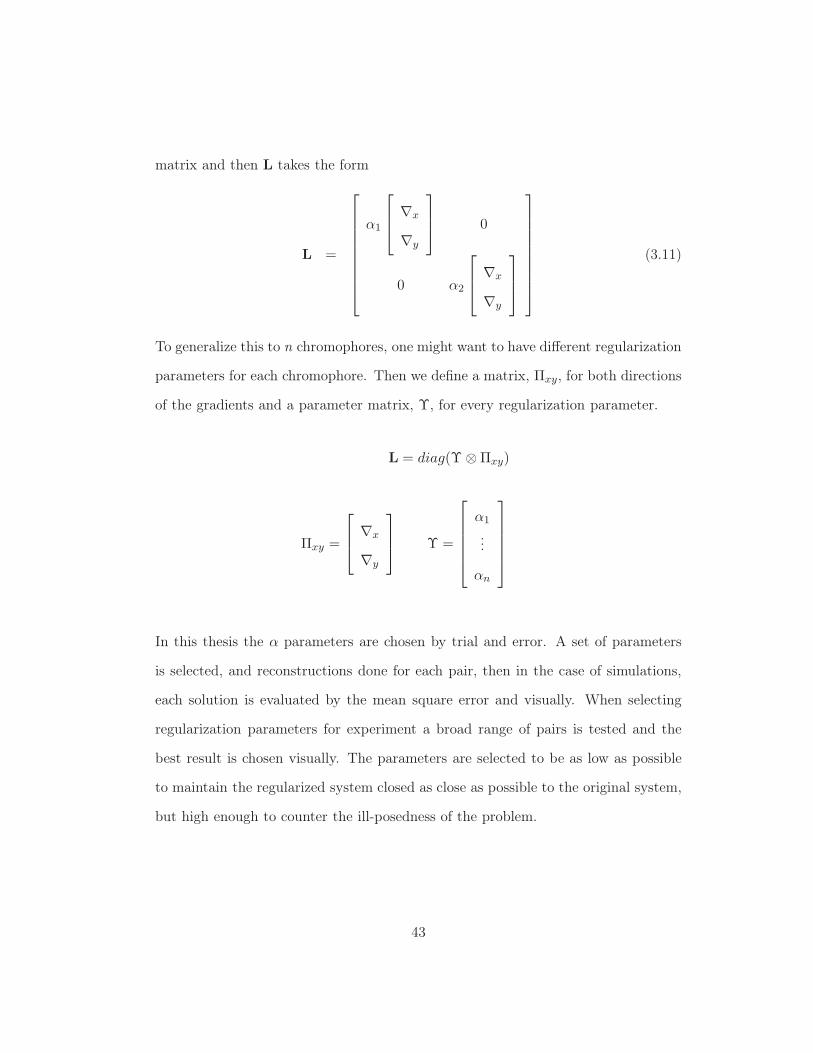
matrix and then L takes the form
L =
⎡⎢⎢⎢⎢⎢⎢⎢⎢⎣
α1
⎡⎢⎣ ∇x
∇y
⎤⎥⎦ 0
0 α2
⎡⎢⎣ ∇x
∇y
⎤⎥⎦
⎤⎥⎥⎥⎥⎥⎥⎥⎥⎦
(3.11)
To generalize this to n chromophores, one might want to have different regularization
parameters for each chromophore. Then we define a matrix, Πxy, for both directions
of the gradients and a parameter matrix, Υ, for every regularization parameter.
L = diag(Υ ⊗ Πxy)
Πxy =
⎡⎢⎣ ∇x
∇y
⎤⎥⎦ Υ =
⎡⎢⎢⎢⎢⎣
α1
...
αn
⎤⎥⎥⎥⎥⎦
In this thesis the α parameters are chosen by trial and error. A set of parameters
is selected, and reconstructions done for each pair, then in the case of simulations,
each solution is evaluated by the mean square error and visually. When selecting
regularization parameters for experiment a broad range of pairs is tested and the
best result is chosen visually. The parameters are selected to be as low as possible
to maintain the regularized system closed as close as possible to the original system,
but high enough to counter the ill-posedness of the problem.
43

3.1.3 Computational issues
Assembly of normal equations and the use of direct methods (SVD, QR, Gaussian
elimination etc.) for their solution is infeasible for 3D problems with hyperspectral
data, especially when one needs to perform these calculation many times in the
evaluation of regularization parameters.
To reduce these computational issues we use iterative methods, specifically
LSQR [JXS+08]. For the case of LSQR, the problem is solved through a method
similar to the conjugate gradient method [PS82]. An interesting feature of this
algorithm is that it interacts with the matrix K only through the matrix vector
products Kf and KT v, for various vectors f and v. For the case of DOT LSQR
becomes highly attractive for its computational efficiency when compared to a direct
solution of traditional least squares. This is due in part to the fact that computing
KTK can require large amounts of computational overhead. The number of voxels
in a given solution becomes somewhat limited by the necessity of solving the system
defined by KTK or some regularized version thereof. Because of the design of K,
as mentioned in Chapter 2, when the voxels increases, the size of KTK and the
computation required for elimination both increase much more rapidly than with
LSQR [PS82].
Solving the regularized version of the system in (3.9) is equivalent to a least
squares solution to the system:
⎡⎢⎣ K
αL
⎤⎥⎦ f =
⎡⎢⎣ g
0
⎤⎥⎦ .
44

We define the augmented weight matrix and data vector as
K =
⎡⎢⎣ K
αL
⎤⎥⎦ g =
⎡⎢⎣ g
0
⎤⎥⎦ .
Using this formulation we can write the problem up as
f̂ = argminf
‖g − Kf‖22. (3.12)
This setup is very attractive for the purpose of this thesis. In this formulation it
is only needed to store one K matrix for each wavelength. This solves the problem
of when using hyperspectral information, the K matrix for all wavelengths would
be too big for computations. The LSQR method allows for using hyperspectral
information meanwhile keeping computations efficient by storing only one K at a
time. This reduces the number of computations immensely. Utilizing the fact that
the iterations compute the matrix vector products KT f and Kf allows us to construct
and store only the K matrix needed for a single wavelength. When the computations
have been done for all wavelengths within each iterations the f vector is updated
when the Kf product is compared to the data vector. This results in working with
very small K matrices at each time compared to if a K matrix would be constructed
for all of the wavelengths wanted in the reconstruction. In the case of hyperspectral
information this becomes very important where the complete K matrix including all
wavelengths would be very big.
Furthermore, sometimes employing a simple LSQR method is not enough.
Because the basic LSQR does not consider any bounds it can sometimes result in
a negative concentrations which are physically impossible. Therefore the NLLS al-
gorithm is used instead of the LSQR method. This is an algorithm included in the
45

MATLAB library and allows me to impose upper and lower bounds on the recon-
struction as well as using a Jacobian in the process. When dealing with measurement
data we used the LSQR method to obtain a reasonable initial guess for the concen-
trations to then put into the NLLS algorithm. This is discussed further in Chapter
5.
46

Chapter 4
Simulations
Simulations are done to test the effect of hyperspectral information when doing
reconstruction of more than one chromophore. To create simulated measurement
data (data that would have obtained from detectors) the reconstruction model is used
to obtain that data from the simulated images. Normally this would be considered
an inverse crime, where numerically produced simulated data is produced by the
same model that is used to invert the data [KS05], but in this case that will be
ignored.
The reason for ignoring this inverse crime is that it is the general consensus
that creating simulated data with the inverse solver is not damaging to results. As
mentioned before there have been claims that a forward solver (predictor) is needed
to simulate data, i.e. it involves predicting the response of a physical system with the
help of some mathematical model incorporating the parameter one wishes to recover
[KS05], [CK92]. Some have proposed that a separate inverse solver (estimator) is
needed to estimate the response of some physical system with the help of another
mathematical model incorporating a variable usually having the same physical and
47

mathematical attributes as the parameter one wishes to recover. It has been shown
that it this separation of predictor and estimator is not necessary to avoid trivial
inversion, in fact it has been derived that might be impossible to obtain a solution,
whose relative error lies below some prescribed threshold, when employing an esti-
mator that is separate to the predictor [Wir08]
.
4.1 Simulated Images
When creating simulated images of two chromophores, images of boxes are created,
a simple one shown in Figure 4.2, to simulate concentration of chromophores. More
complex chromophore images are shown in Figures 4.3 and 4.4.
Information for the background from is taken literature. It is assumed that
the μ′s follows Mie Scattering theory. A scattering prefactor Ψ depends primarily on
the number and size of scatterers, and a scattering exponent b depends on the size
of scatterers [KCC+08]. This is combined as:
μ′s = Ψλ−b (4.1)
Values for Ψ and b are obtained from [TPT+03] for the breast. Values for μa are
obtained from [SB81], which are values in the 600-900 nm range in 10 nm intervals.
For wavelengths between those intervals we interpolate between values from the
article.
For the concentration defined in the simulated images it is defined units of
molarity or mol per liter, M. The extinction coefficients for each chromophore are in
the units cm−1/M and are obtained from Scott Prahl of the Oregon Medical Laser
48

650 700 750 800 850 9000
500
1000
1500
2000
2500
3000
3500
4000
Mol
ar e
xtin
ctio
n co
effic
ient
[cm
−1 /M
]
Wavelengths [nm]
HbO
2
HbR
Figure 4.1: Molar extinction coefficents used in simulations plotted as a function ofwavelength.
Center [Pra]. The extinction coefficients are shown in Figure 4.1.
Three different sets of images are created to test the reconstruction. The
first set is a simple image with only a concentration for HbO2 and none for HbR.
Reconstruction is done for these images to explore effects of adding hyperspectral
information to the problem, i.e. the reduction of crosstalk where a concentration of
one chromophore creates a false concentration in an image for another chromophore.
The second set is a little more complex with concentrations of HbR in different areas
than HbO2. The third set is more complicated with concentrations for HbO2 and
HbR in the same areas. In the third set the intensity of the concentrations are not
the same for the two chromophores. These images are shown in Figures 4.2-4.4.
The alignment of sources and detectors with the respect of the simulated images is
displayed in Figure 4.5.
In simulations the forward model is used to create data from the images. This
is done by doing the following process,
g = K
⎡⎢⎣ fCP1
fCP2
⎤⎥⎦ + n (4.2)
49

cm
cm
2 4 6 8 10
1
2
3
4
5
6
7
8
9
100
0.1
0.2
0.3
0.4
0.5
0.6
0.7
0.8
0.9
1
cm
cm
1 2 3 4 5 6 7 8 9 10
1
2
3
4
5
6
7
8
9
100
0.1
0.2
0.3
0.4
0.5
0.6
0.7
0.8
0.9
1
Figure 4.2: Simple concentration images for a single chromophore. Left image is forHbO2 and right image is for HbR.
cm
cm
2 4 6 8 10
1
2
3
4
5
6
7
8
9
100
0.1
0.2
0.3
0.4
0.5
0.6
0.7
0.8
0.9
1
cm
cm
2 4 6 8 10
1
2
3
4
5
6
7
8
9
100
0.1
0.2
0.3
0.4
0.5
0.6
0.7
0.8
0.9
1
Figure 4.3: Images with concentrations for two chromophores. Left image is forHbO2 and right image is for HbR.
cm
cm
0 2 4 6 8 10
0
1
2
3
4
5
6
7
8
9
100
0.1
0.2
0.3
0.4
0.5
0.6
0.7
0.8
0.9
1
cm
cm
0 2 4 6 8 10
0
1
2
3
4
5
6
7
8
9
100
0.1
0.2
0.3
0.4
0.5
0.6
0.7
0.8
0.9
1
Figure 4.4: Images with concentrations for two chromophores with different intensi-ties. Left image is for HbO2 and right image is for HbR.
50

Figure 4.5: The setup of sources and detectors.
where fCP1 and fCP2 are the simulated concentration images for each chromophore.
After this, data vector is created and noise is added to it in the range of 60-120 dB.
The SNR of adding this noise will be calculated by using the following equation
SNR = 10log10
‖g‖2
Nσ2(4.3)
where N is the number of data points and g is the signal with out additive noise.
Because phantoms are assumed to be infinite in the z -direction, 50 z -planes are used
when creating the simulated data. The images are created to test the inverse solution
with respect to spectral information, regularization, cross-talk and accuracy. To es-
timate the effectiveness of the reconstruction in simulations, for the nth chromophore
the mean square error is computed by using the following equation
MSECPn =‖fCPn − f̂CPn‖2
‖fCPn‖2, (4.4)
51
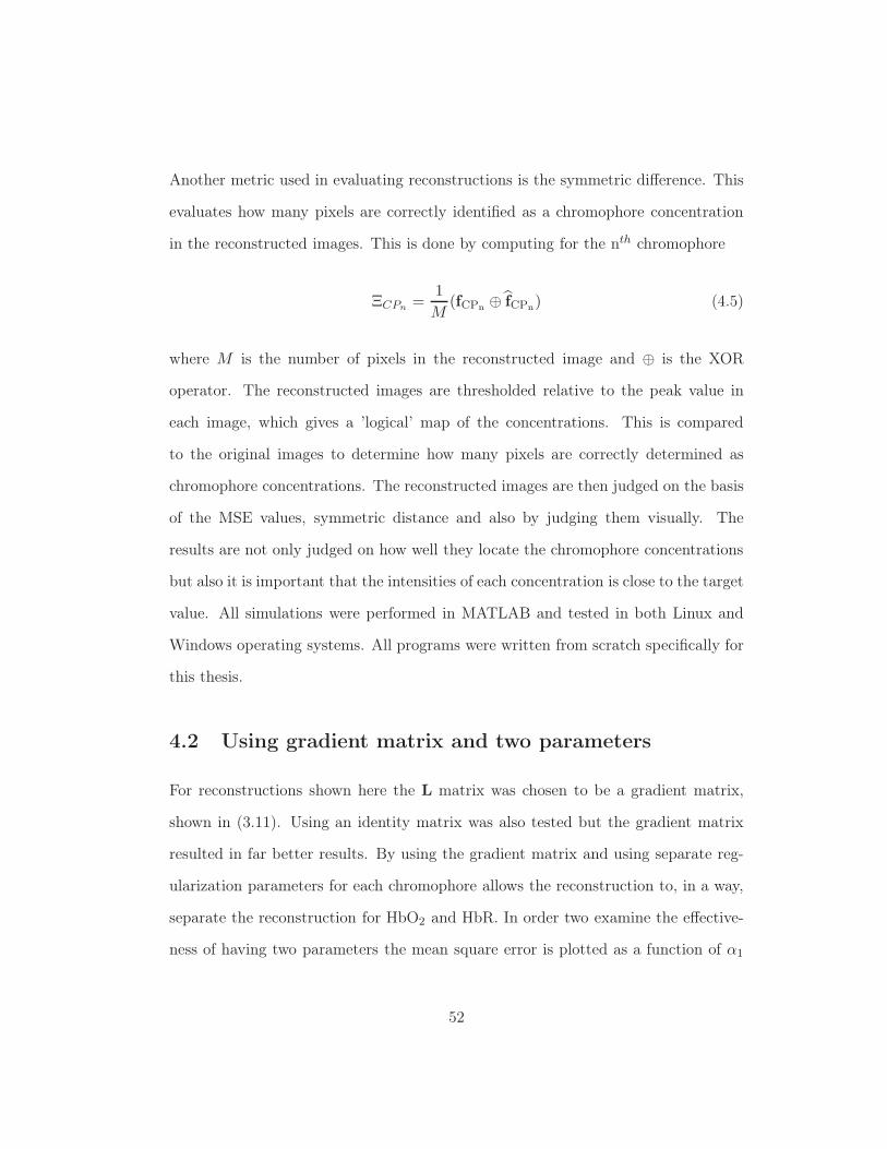
Another metric used in evaluating reconstructions is the symmetric difference. This
evaluates how many pixels are correctly identified as a chromophore concentration
in the reconstructed images. This is done by computing for the nth chromophore
ΞCPn =1M
(fCPn ⊕ f̂CPn) (4.5)
where M is the number of pixels in the reconstructed image and ⊕ is the XOR
operator. The reconstructed images are thresholded relative to the peak value in
each image, which gives a ’logical’ map of the concentrations. This is compared
to the original images to determine how many pixels are correctly determined as
chromophore concentrations. The reconstructed images are then judged on the basis
of the MSE values, symmetric distance and also by judging them visually. The
results are not only judged on how well they locate the chromophore concentrations
but also it is important that the intensities of each concentration is close to the target
value. All simulations were performed in MATLAB and tested in both Linux and
Windows operating systems. All programs were written from scratch specifically for
this thesis.
4.2 Using gradient matrix and two parameters
For reconstructions shown here the L matrix was chosen to be a gradient matrix,
shown in (3.11). Using an identity matrix was also tested but the gradient matrix
resulted in far better results. By using the gradient matrix and using separate reg-
ularization parameters for each chromophore allows the reconstruction to, in a way,
separate the reconstruction for HbO2 and HbR. In order two examine the effective-
ness of having two parameters the mean square error is plotted as a function of α1
52

and α2. Plotting this produces a three dimensional surface which shows the optimal
parameters, where the mean square error is minimized. The MSE is the then com-
puted using (4.4). Plots for the mean square error for the first set is shown in Figure
4.6. From these plots it is possible to determine an optimal value for α1 and α2.
For a simple chromophore concentrations like in the first set, choosing the regular-
ization parameters is an easy problem. The reason for separating the regularization
parameters in this case is that the MSE for HbR reaches a lower value for a higher
α1 than HbO2 and as mentioned in Chapter 3 the best choice for the parameters is
the lowest choice possible. Although keeping the parameters separate is useful for
multiple chromophore, it could be seen from the plot in Figure 4.6 that α1 could
be equal to α2. This is because in this case only one chromophore is being recon-
structed, so it is much easier to find an optimal value for the parameter regularizing
the "missing" chromophore. Examining the results visually shows that separating
them gives better results. The importance of separating the regularization parame-
ters becomes even more visible when regularizing more complex concentration sets.
In Figure 4.7 it shows that the lowest MSE values for HbO2 and HbR occur at two
very different values. For this set the separation of the regularization parameters is
very important. Using only one regularization parameter in this set and more com-
plicated ones, would result in a trade off between reconstructions of chromophores.
To reduce that trade off the separation of the chromophores becomes very important.
This separation becomes even more important when dealing with data sets with low
SNR values such as true measurement data.
53

100200
300400
500600
700800
900
100
200
300
400
500
600
700
800
900
1.5
2
2.5
3
3.5
4
4.5
5
5.5
6
6.5
α1α
2
MS
E
100200
300400
500600
700800
900
100
200
300
400
500
600
700
800
900
0
0.5
1
1.5
2
2.5
3
3.5
4
4.5
5
α1α
2
MS
EFigure 4.6: Mean square error as function of regularization parameters for the firstset. Left image is HbO2 and right image is HbR.
2
4
6
8
10
x 105
12
34
56
78
910
x 105
0.8
1
1.2
1.4
1.6
1.8
2
2.2
α1α
2
MS
E
2
4
6
8
10
x 105
12
34
56
78
910
x 105
0.65
0.7
0.75
0.8
0.85
0.9
0.95
1
α1α
2
MS
E
Figure 4.7: Mean square error as function of regularization parameters for the secondset. Left image is HbO2 and right image is HbR.
4.3 Reconstruction
The main goal is to show the advantage of hyperspectral information. The in-
creased number of wavelengths should make the inverse problem less ill-posed and
54

reduce cross-talk between chromophores. First we will display simple images to show
these advantages and then show examples for more complicated images. Although
crosstalk can in most cases be eliminated completely it is greatly reduced by using
a very high number of wavelengths.
4.3.1 First set
In reconstructions done for the images in Figure 4.8, noticeable crosstalk is present
when few wavelengths are used. Using few wavelengths results in a diffuse recon-
struction of the HbO2 concentration. This result also shows evidence of HbR, which
is a result of cross-talk. Increasing the number of wavelengths to 26 wavelengths
gives somewhat better results. The jump from 6 wavelengths to 26 wavelengths is
not significant but some reduction in cross-talk is evident and better definition of
the HbO2 concentration is obtained.
In Figure 4.9 results are shown for 126 wavelengths and 251 wavelengths.
This shows a significant improvement in reconstructions for both chromophores. In
the 126 wavelengths case the cross-talk is almost vanished and the HbO2 concentra-
tions is better defined and approaching the correct intensity values. Moving to 251
wavelengths shows a very good reconstruction with a good approximation of HbO2
and negligible crosstalk.
In Figure 4.10 the MSE is plotted as a function wavelengths to show how
hyperspectral information results in better reconstructions. The MSE values show
that the accuracy increases greatly when wavelengths are added. The trend for
HbR shows small changes as there is no chromophore to reconstruct, but crosstalk
is shown to be reduced.
Examining the symmetric difference in Figure 4.11 the HbR reconstructions
55

are well described. The improvement is not much, no chromophore present, but the
difference decreases a little bit when the cross-talk is eliminated more and more. As
with the MSE the improvement for HbO2 is clear.
4.3.2 Second set
Examining reconstructions at few wavelengths are shown in Figure 4.12. A good
approximation is obtained for HbR but HbO2 results in a blurry reconstruction. It
is noticeable for both the 6 and 26 wavelength cases that noticeable cross-talk is
evident in the HbR images. The effects of the HbO2 concentrations are appearing in
the HbR images, same as what happened in the first set. Increasing the wavelengths
to 26 wavelengths gives a better results for HbO2 but remains blurry.
Using 126 and 251 wavelengths, shown in Figure 4.13, the cross-talk in the
HbR image is reduced. As in the first set the reconstruction for HbO2 is greatly
improved. A very good approximation of both chromophores is shown for 251 wave-
lengths. Even using 126 wavelengths the localization of HbO2 is better and ap-
proaching the correct intensity.
The improvement in using hyperspectral information is shown in the MSE
values, Figure 4.14. The localization of HbR remains good with all wavelengths
resulting in a small increase of the symmetric difference, Figure 4.15, for the HbR.
The decrease in that case is due to the reduction of cross talk. The symmetric
difference significantly decreases when more wavelengths are added as expected when
the images become more accurate.
56

cm
cm
2 4 6 8 10
1
2
3
4
5
6
7
8
9
100
0.1
0.2
0.3
0.4
0.5
0.6
0.7
0.8
0.9
1
cm
cm
0 2 4 6 8 10
0
1
2
3
4
5
6
7
8
9
100
0.1
0.2
0.3
0.4
0.5
0.6
0.7
0.8
0.9
1
cm
cm
0 2 4 6 8 10
0
1
2
3
4
5
6
7
8
9
100
0.1
0.2
0.3
0.4
0.5
0.6
0.7
0.8
0.9
1
cm
cm
1 2 3 4 5 6 7 8 9 10
1
2
3
4
5
6
7
8
9
100
0.1
0.2
0.3
0.4
0.5
0.6
0.7
0.8
0.9
1
cm
cm
0 2 4 6 8 10
0
1
2
3
4
5
6
7
8
9
100
0.1
0.2
0.3
0.4
0.5
0.6
0.7
0.8
0.9
1
cm
cm
0 2 4 6 8 10
0
1
2
3
4
5
6
7
8
9
100
0.1
0.2
0.3
0.4
0.5
0.6
0.7
0.8
0.9
1
Figure 4.8: Reconstruction for first set, low complexity. Middle images is done with6 wavelengths and rightmost images is done with 26 wavelengths. Upper row is forthe HbO2 chromophore and the lower for HbR. SNR is 64.9 dB.
cm
cm
2 4 6 8 10
1
2
3
4
5
6
7
8
9
100
0.1
0.2
0.3
0.4
0.5
0.6
0.7
0.8
0.9
1
cm
cm
0 2 4 6 8 10
0
1
2
3
4
5
6
7
8
9
100
0.1
0.2
0.3
0.4
0.5
0.6
0.7
0.8
0.9
1
cm
cm
0 2 4 6 8 10
0
1
2
3
4
5
6
7
8
9
100
0.1
0.2
0.3
0.4
0.5
0.6
0.7
0.8
0.9
1
cm
cm
1 2 3 4 5 6 7 8 9 10
1
2
3
4
5
6
7
8
9
100
0.1
0.2
0.3
0.4
0.5
0.6
0.7
0.8
0.9
1
cm
cm
0 2 4 6 8 10
0
1
2
3
4
5
6
7
8
9
100
0.1
0.2
0.3
0.4
0.5
0.6
0.7
0.8
0.9
1
cm
cm
0 2 4 6 8 10
0
1
2
3
4
5
6
7
8
9
100
0.1
0.2
0.3
0.4
0.5
0.6
0.7
0.8
0.9
1
Figure 4.9: Reconstruction for first set, low complexity. Middle images is done with126 wavelengths and rightmost images is done with 251 wavelengths. Upper row isfor the HbO2 chromophore and the lower for HbR. SNR is 63.9 dB.
57

0 50 100 150 200 250 3000
0.5
1
1.5
2
2.5
3
3.5
4
4.5
Number of Wavelengths
MS
E
HbO
2
HbR
Figure 4.10: MSE plotted as a function of the number of wavelengths for the first set.
0 50 100 150 200 250 3000
0.05
0.1
0.15
0.2
0.25
0.3
0.35
0.4
# of wavelengths
Sym
met
ric D
ista
nce
HbO
2
HbR
Figure 4.11: Symmetric difference plotted as a function of the number of wavelengthsfor the first set.
4.3.3 Third set
In Figure 4.16 the reconstruction for the HbO2 fails almost completely. Although
the reconstruction show good results for HbR the HbO2 concentrations are far off
the true values. When increasing number of wavelengths to 26 the localization HbO2
are somewhat better but the intensities are far off.
Using hyperspectral information, Figure 4.17, results in much better recon-
structions. For 126 wavelengths the separation of the two concentrations in the HbO2
case becomes better defined. In the 251 wavelength case a good approximation for
58

cm
cm
2 4 6 8 10
1
2
3
4
5
6
7
8
9
100
0.1
0.2
0.3
0.4
0.5
0.6
0.7
0.8
0.9
1
cm
cm
0 2 4 6 8 10
0
1
2
3
4
5
6
7
8
9
100
0.1
0.2
0.3
0.4
0.5
0.6
0.7
0.8
0.9
1
cm
cm
0 2 4 6 8 10
0
1
2
3
4
5
6
7
8
9
100
0.1
0.2
0.3
0.4
0.5
0.6
0.7
0.8
0.9
1
cm
cm
2 4 6 8 10
1
2
3
4
5
6
7
8
9
100
0.1
0.2
0.3
0.4
0.5
0.6
0.7
0.8
0.9
1
cm
cm
0 2 4 6 8 10
0
1
2
3
4
5
6
7
8
9
100
0.1
0.2
0.3
0.4
0.5
0.6
0.7
0.8
0.9
1
cm
cm
0 2 4 6 8 10
0
1
2
3
4
5
6
7
8
9
100
0.1
0.2
0.3
0.4
0.5
0.6
0.7
0.8
0.9
1
Figure 4.12: Reconstruction for second set, medium complexity. Middle images isdone with 6 wavelengths and rightmost images is done with 26 wavelengths. Upperrow is for the HbO2 chromophore and the lower for HbR. SNR is 83.6 dB.
cm
cm
2 4 6 8 10
1
2
3
4
5
6
7
8
9
100
0.1
0.2
0.3
0.4
0.5
0.6
0.7
0.8
0.9
1
cm
cm
0 2 4 6 8 10
0
1
2
3
4
5
6
7
8
9
100
0.1
0.2
0.3
0.4
0.5
0.6
0.7
0.8
0.9
1
cm
cm
0 2 4 6 8 10
0
1
2
3
4
5
6
7
8
9
100
0.1
0.2
0.3
0.4
0.5
0.6
0.7
0.8
0.9
1
cm
cm
2 4 6 8 10
1
2
3
4
5
6
7
8
9
100
0.1
0.2
0.3
0.4
0.5
0.6
0.7
0.8
0.9
1
cm
cm
0 2 4 6 8 10
0
1
2
3
4
5
6
7
8
9
100
0.1
0.2
0.3
0.4
0.5
0.6
0.7
0.8
0.9
1
cm
cm
0 2 4 6 8 10
0
1
2
3
4
5
6
7
8
9
100
0.1
0.2
0.3
0.4
0.5
0.6
0.7
0.8
0.9
1
Figure 4.13: Reconstruction for second set, medium complexity. Middle images isdone with 126 wavelengths and rightmost images is done with 251 wavelengths. Upperrow is for the HbO2 chromophore and the lower for HbR. SNR is 90.6 dB.
59

0 50 100 150 200 250 300
0.4
0.5
0.6
0.7
0.8
0.9
1
Number of Wavelengths
MS
E
HbO
2
HbR
Figure 4.14: MSE plotted as a function of the number of wavelengths for the secondset.
0 50 100 150 200 250 3000
0.05
0.1
0.15
0.2
0.25
0.3
0.35
0.4
0.45
0.5
# of wavelengths
Sym
met
ric D
ista
nce
HbO
2
HbR
Figure 4.15: Symmetric difference plotted as a function of the number of wavelengthsfor the second set.
both chromophore is reached.
This improvement in reconstruction is shown for both chromophores in Figure
4.18 and the improvement of the localization of HbO2 is evident in Figure 4.19. As
in the second set the localization of the HbR is acceptable for all wavelength cases.
60

cm
cm
0 2 4 6 8 10
0
1
2
3
4
5
6
7
8
9
100
0.1
0.2
0.3
0.4
0.5
0.6
0.7
0.8
0.9
1
cm
cm
0 2 4 6 8 10
0
1
2
3
4
5
6
7
8
9
100
0.1
0.2
0.3
0.4
0.5
0.6
0.7
0.8
0.9
1
cm
cm
0 2 4 6 8 10
0
1
2
3
4
5
6
7
8
9
100
0.1
0.2
0.3
0.4
0.5
0.6
0.7
0.8
0.9
1
cm
cm
0 2 4 6 8 10
0
1
2
3
4
5
6
7
8
9
100
0.1
0.2
0.3
0.4
0.5
0.6
0.7
0.8
0.9
1
cm
cm
0 2 4 6 8 10
0
1
2
3
4
5
6
7
8
9
100
0.1
0.2
0.3
0.4
0.5
0.6
0.7
0.8
0.9
1
cm
cm
0 2 4 6 8 10
0
1
2
3
4
5
6
7
8
9
100
0.1
0.2
0.3
0.4
0.5
0.6
0.7
0.8
0.9
1
Figure 4.16: Reconstruction for third set, high complexity. Middle images is donewith 6 wavelengths and rightmost images is done with 26 wavelengths. Upper row isfor the HbO2 chromophore and the lower for HbR. SNR is 80.7 dB.
cm
cm
0 2 4 6 8 10
0
1
2
3
4
5
6
7
8
9
100
0.1
0.2
0.3
0.4
0.5
0.6
0.7
0.8
0.9
1
cm
cm
0 2 4 6 8 10
0
1
2
3
4
5
6
7
8
9
100
0.1
0.2
0.3
0.4
0.5
0.6
0.7
0.8
0.9
1
cm
cm
0 2 4 6 8 10
0
1
2
3
4
5
6
7
8
9
100
0.1
0.2
0.3
0.4
0.5
0.6
0.7
0.8
0.9
1
cm
cm
0 2 4 6 8 10
0
1
2
3
4
5
6
7
8
9
100
0.1
0.2
0.3
0.4
0.5
0.6
0.7
0.8
0.9
1
cm
cm
0 2 4 6 8 10
0
1
2
3
4
5
6
7
8
9
100
0.1
0.2
0.3
0.4
0.5
0.6
0.7
0.8
0.9
1
cm
cm
0 2 4 6 8 10
0
1
2
3
4
5
6
7
8
9
100
0.1
0.2
0.3
0.4
0.5
0.6
0.7
0.8
0.9
1
Figure 4.17: Reconstruction for third set, high complexity. Middle images is donewith 126 wavelengths and rightmost images is done with 251 wavelengths. Upper rowis for the HbO2 chromophore and the lower for HbR. SNR is 85.5 dB
61

0 50 100 150 200 250 300
0.4
0.5
0.6
0.7
0.8
0.9
1
Number of Wavelengths
MS
E
HbO
2
HbR
Figure 4.18: MSE plotted as a function of the number of wavelengths for the thirdset.
0 50 100 150 200 250 3000.1
0.2
0.3
0.4
0.5
0.6
0.7
0.8
# of wavelengths
Sym
met
ric D
ista
nce
HbO
2
HbR
Figure 4.19: Symmetric difference plotted as a function of the number of wavelengthsfor the third set.
62

Chapter 5
Physical Measurements
In order to test the simulation results, physical measurements were performed. The
goal of the measurement were to show how hyperspectral information gives way to
the imaging of two different chromophores by using the direct method.
5.1 Measurement Process
The process can be divided into four parts.
1. Construction and measurement of the actual phantoms,
2. Construction of the medium
3. Measurement of the background
4. Measurement of the phantoms in the medium
Each process will be discussed in this section along with measurement results com-
pared to simulations.
63
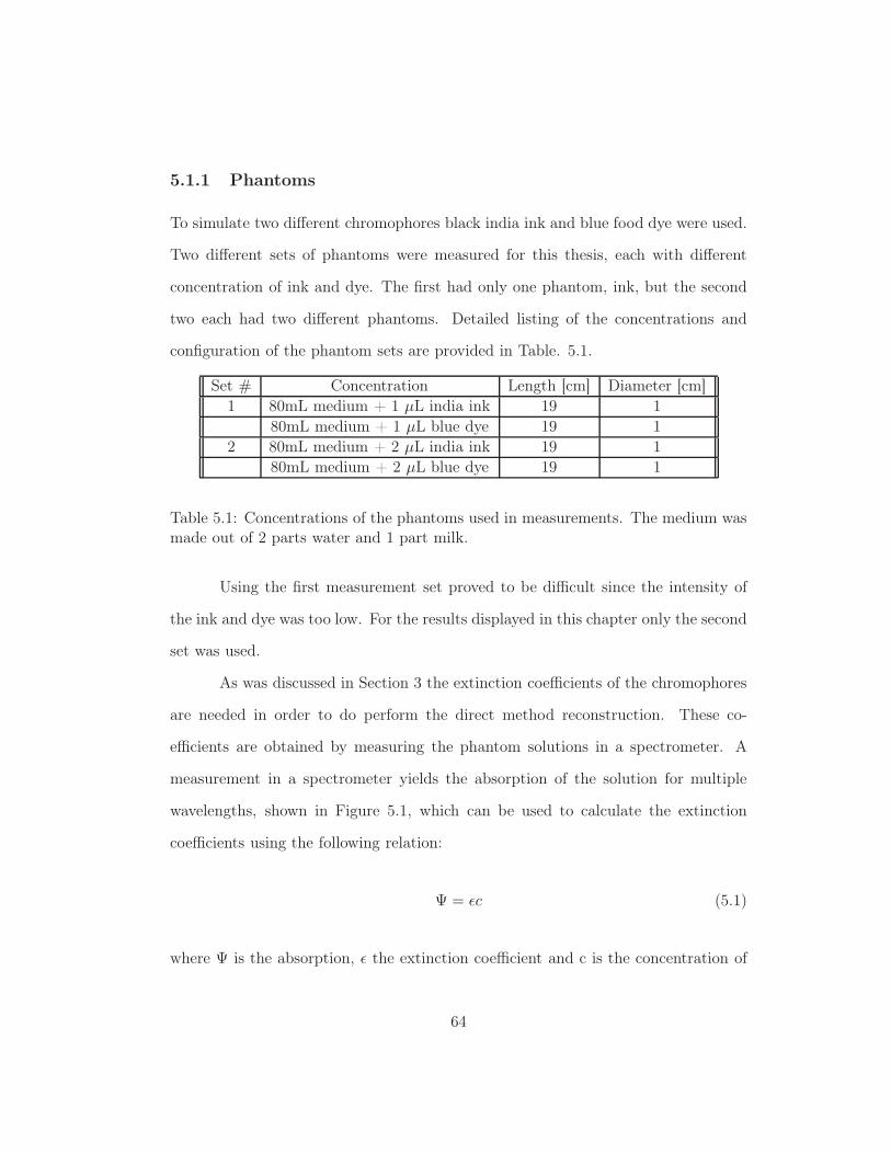
5.1.1 Phantoms
To simulate two different chromophores black india ink and blue food dye were used.
Two different sets of phantoms were measured for this thesis, each with different
concentration of ink and dye. The first had only one phantom, ink, but the second
two each had two different phantoms. Detailed listing of the concentrations and
configuration of the phantom sets are provided in Table. 5.1.
Set # Concentration Length [cm] Diameter [cm]1 80mL medium + 1 μL india ink 19 1
80mL medium + 1 μL blue dye 19 12 80mL medium + 2 μL india ink 19 1
80mL medium + 2 μL blue dye 19 1
Table 5.1: Concentrations of the phantoms used in measurements. The medium wasmade out of 2 parts water and 1 part milk.
Using the first measurement set proved to be difficult since the intensity of
the ink and dye was too low. For the results displayed in this chapter only the second
set was used.
As was discussed in Section 3 the extinction coefficients of the chromophores
are needed in order to do perform the direct method reconstruction. These co-
efficients are obtained by measuring the phantom solutions in a spectrometer. A
measurement in a spectrometer yields the absorption of the solution for multiple
wavelengths, shown in Figure 5.1, which can be used to calculate the extinction
coefficients using the following relation:
Ψ = εc (5.1)
where Ψ is the absorption, ε the extinction coefficient and c is the concentration of
64

the subject at hand. It should be noted that when the solutions are measured in
the spectrometer milk is not used. This is due to the fact that absorption cannot
be measured with milk in the medium since the light in the spectrometer would be
fully absorbed by the milk. Because of the similarities in the spectra of milk and
water this does not cause big errors in calculation of the extinction coefficients. In
measurements the unit of the extinction coefficients are 1/cm.
450 500 550 600 650 7000
0.5
1
1.5
2
2.5
Wavelengths [nm]
Abs
orpt
ion
India InkBlue Dye
(a)
450 500 550 600 650 7000
0.5
1
1.5
2
2.5
3
Wavelengths [nm]
Abs
orpt
ion
India Ink
Blue Dye
(b)
Figure 5.1: (a) Absorption spectra for set #1.(b)Absorption spectra for set #2.
It should also be noted that the actual intensity of the ink concentration is
relatively small. That is because if too much ink is put into the phantom, it will
absorb all the light passing through it and no spectral information will reach the
detector. So a fine line has to be tread when creating the phantoms, keeping the
intensities low enough so that spectral information can be obtained, but still having
them as strong as possible so that they can be seen reconstructed images.
5.1.2 Background
The medium is constructed using milk and water. Milk, with 2% fat, is used due to
the similarities of the optical properties to human skin. A tank is filled with 7 liters
of milk and 14 liters of water so that the ratio between water and milk is 2:1.
65
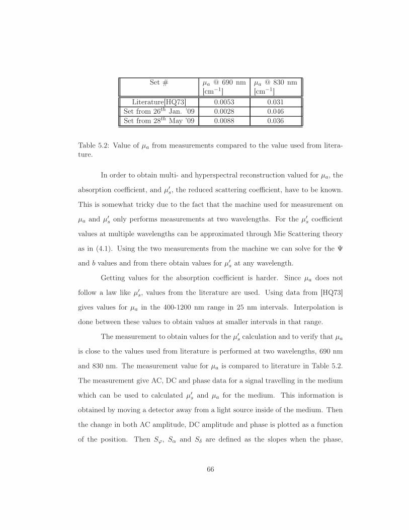
Set # μa @ 690 nm[cm−1]
μa @ 830 nm[cm−1]
Literature[HQ73] 0.0053 0.031Set from 26th Jan. ’09 0.0028 0.046Set from 28th May ’09 0.0088 0.036
Table 5.2: Value of μa from measurements compared to the value used from litera-ture.
In order to obtain multi- and hyperspectral reconstruction valued for μa, the
absorption coefficient, and μ′s, the reduced scattering coefficient, have to be known.
This is somewhat tricky due to the fact that the machine used for measurement on
μa and μ′s only performs measurements at two wavelengths. For the μ′
s coefficient
values at multiple wavelengths can be approximated through Mie Scattering theory
as in (4.1). Using the two measurements from the machine we can solve for the Ψ
and b values and from there obtain values for μ′s at any wavelength.
Getting values for the absorption coefficient is harder. Since μa does not
follow a law like μ′s, values from the literature are used. Using data from [HQ73]
gives values for μa in the 400-1200 nm range in 25 nm intervals. Interpolation is
done between these values to obtain values at smaller intervals in that range.
The measurement to obtain values for the μ′s calculation and to verify that μa
is close to the values used from literature is performed at two wavelengths, 690 nm
and 830 nm. The measurement value for μa is compared to literature in Table 5.2.
The measurement give AC, DC and phase data for a signal travelling in the medium
which can be used to calculated μ′s and μa for the medium. This information is
obtained by moving a detector away from a light source inside of the medium. Then
the change in both AC amplitude, DC amplitude and phase is plotted as a function
of the position. Then Sϕ, Sα and Sδ are defined as the slopes when the phase,
66

ln(DC · r) and ln(AC · r) are plotted respectively as a function of position of r the
source-detector separation. The absorption coefficient and scattering coefficient can
then be calculated from Sα by using
μa =ω
2υ
(Sϕ
Sα− Sα
Sϕ
)μ′
s =S2
α − S2ϕ
3μa.
where ω is the modulation frequency set at 110 MHz, υ is the speed of light divided
by the index of refraction [FFFG94]. Using Sδ these values can be verified by using
these relations
μa = − ω
2υ
(S2ϕ
S2δ
+ 1)− 1
2μ′
s =S2
δ
3μa− μa
The values of μa are then compared to literature values in Table 5.2 and used to
compute μ′s with (4.1). As can be seen in Table 5.2 the value at 690 nm is not as close
as the one for 830 nm. Although this introduces some error in the reconstruction
it is the only way to obtain hyperspectral information regarding μa since the onsite
machine only takes measurement at two values. Constructing weight matrices for
different μa values showed that the error in μa should not be expected to dominate
the reconstructions.
5.1.3 Spectrograph
When phantoms have been constructed and all the necessary background measure-
ments have been taken of the medium, the final step is to actually perform the
measurement. A single source and a single detector are placed in the medium on
opposite sides of the phantoms. Then the detector takes measurements at multiple
67

cm
cm
0 1 2 3 4 5 6 7
0
0.5
1
1.5
2
0
0.2
0.4
0.6
0.8
1x 10
−5
cm
cm
0 1 2 3 4 5 6 7
0
0.5
1
1.5
2
0
0.2
0.4
0.6
0.8
1x 10
−5
Figure 5.2: Target image for the first measurement taken on January 28th 2009.This is using only a single ink phantom from set #2. Upper image is for ink andlower image is for dye.
points for each location of the source. This gives a tomographic data set that can
be used for reconstruction and source-detector pairs were used in the range from 30
to around 100.
The results displayed are from two data sets. First set was taken on January
28th 2009. A single phantom was used, from set #1 in Table 5.1. A total of 6
sources and 10 detectors were placed 4 cm apart to result in a 60 source/detector
pair tomographic data. The other two sets were taken on May 28th 2009. The second
set has two phantoms, one ink and one dye separated by 4 cm. A total of 9 sources
and 11 detectors were placed 4.5 cm apart resulting in 99 source/detector pairs. For
each measurement set we created target images which show what is expected to get
from the reconstructed images. These images are shown for each set in Figures 5.2
68

cm
cm
0 1 2 3 4 5 6 7
0
0.5
1
1.5
2
0
0.2
0.4
0.6
0.8
1x 10
−5
cm
cm
0 1 2 3 4 5 6 7
0
0.5
1
1.5
2
0
0.2
0.4
0.6
0.8
1x 10
−5
Figure 5.3: Target image for the first measurement taken on May 28th 2009. Bothink and dye phantoms from set #2 were used. Upper image is for ink and lowerimage is for dye.
to 5.3.
5.2 Results
In this section we will show the reconstructed images obtained from experiment
data. The results will be judged by using the MSE value and visually as before.
Additionally we examine how effective the method is in localizing the concentrations
by examining only the boundary of reconstructed concentrations and the symmetric
difference between the target image and the reconstructed image.
69

5.2.1 First set
In this case there is only the ink phantom from set #3, shown in table 5.1. With 2
μL of ink in 80 mL solutions the target concentrations are 2.5 ∗ 10−5%. Initially re-
construction was tried by using zero as an initial guess in the NLLS algorithm. This
proved to be unsuccessful resulting in unusable images. After trying many regular-
ization parameters, an initial guess was obtained by running the LSQR algorithm.
Images obtained from that resulted in some negative values, which is of course not
possible with a physical concentration. This result was then used as an initial guess
for the NLLS algorithm by setting negative values to zero which resulted in better
reconstructions. The NLLS algorithm allows me to put on upper and lower bounds
for the reconstruction since the concentrations should be between zero and 1, since
in the measurement the concentrations are a percentages.
Reconstruction for 3 wavelengths is shown in Figure 5.4. This reconstruction
resulted with some reconstruction for ink and almost none for the dye chromophore.
Although it gives some concentration for the ink, the spread of the ink is considerable
and bigger than expected. Additionally to that, there is noticeable interference
from the outermost sources and detectors. The singularity of the Green’s function,
in (2.12), creates these artifacts. Although regularization parameters were set so
that these interference were as little as possible it is very hard to get rid of them
completely.
Increasing the number of wavelengths results in better reconstructions as
shown in Figure 5.5. This reconstruction is done with 6 wavelengths and locates the
phantom very well. it is noticeable that increasing the wavelengths further than 6
wavelengths results in very similar results. The reconstruction at 13 wavelengths in
Figure 5.6 shows similar results. Increasing the number of wavelengths to 26, Figure
70

cm
cm
0 1 2 3 4 5 6 7
0
0.5
1
1.5
2 0.5
1
1.5
2
2.5
3
3.5
4
x 10−7
cm
cm
0 1 2 3 4 5 6 7
0
0.5
1
1.5
2 0.5
1
1.5
2
2.5
3
3.5
4
x 10−7
Figure 5.4: Reconstruction done for a single ink phantom. 3 wavelengths and 21z-planes used. Upper image is for ink and lower image is for dye.
cm
cm
0 1 2 3 4 5 6 7
0
0.5
1
1.5
2 0.5
1
1.5
2
2.5
3
3.5
x 10−7
cm
cm
0 1 2 3 4 5 6 7
0
0.5
1
1.5
2 0.5
1
1.5
2
2.5
3
3.5
x 10−7
Figure 5.5: Reconstruction done for a single ink phantom. 6 wavelengths and 21z-planes used. Upper image is for ink and lower image is for dye.
71

cm
cm
0 1 2 3 4 5 6 7
0
0.5
1
1.5
2 0.5
1
1.5
2
2.5
3
x 10−7
cm
cm
0 1 2 3 4 5 6 7
0
0.5
1
1.5
2 0.5
1
1.5
2
2.5
3
x 10−7
Figure 5.6: Reconstruction done for a single ink phantom. 13 wavelengths and 21z-planes used. Upper image is for ink and lower image is for dye.
cm
cm
0 1 2 3 4 5 6 7
0
0.5
1
1.5
2 0.5
1
1.5
2
2.5
3
3.5
x 10−7
cm
cm
0 1 2 3 4 5 6 7
0
0.5
1
1.5
2 0.5
1
1.5
2
2.5
3
3.5
x 10−7
Figure 5.7: Reconstruction done for a single ink phantom. 26 wavelengths and 21z-planes used. Upper image is for ink and lower image is for dye.
72

5.7, creates a more accurate image where the concentration of ink is more localized to
the expected region. As can be seen the singularities due to the outermost detectors
were somewhat reduced. Although the accuracy is not increase greatly by the adding
of wavelengths it is noticeable that the reconstruction approaches the target value
when the number of wavelengths is increased. This is also reconstruction done for a
single chromophore so the issues of cross-talk is not noticeable.
0 5 10 15 20 25 300.9975
0.998
0.9985
0.999
0.9995
1
Number of Wavelengths
MS
E
Ink
Figure 5.8: MSE displayed for second measurement set for ink at every wavelength.
In Figure 5.8 the mean square error is shown for each reconstruction as a
function of wavelength. This gives a good idea how the reconstruction is better
when multiple wavelengths are used. Examining the symmetric difference in Figure
5.9 it is evident that it follows the same trend as the MSE in Figure 5.8, that a
good result is obtained by using 6 wavelengths. It should be emphasized that this is
reconstruction only done for a single chromophore, so there is very little cross-talk to
deal with. The localization of the phantom is also emphasized in Figure 5.10 where
it is shown how effectively the reconstruction located the phantom by drawing the
boundaries of the reconstructed concentrations compared to the target image.
73

3 4 5 6 7 8 9 10 11 12 130.05
0.06
0.07
0.08
0.09
0.1
0.11
0.12
0.13
# of wavelengths
Sym
met
ric D
ista
nce
Ink
Figure 5.9: The symmetrical difference of reconstructions for the first set plotted asa function wavelength.
cm
cm
0 1 2 3 4 5 6 7
0
0.2
0.4
0.6
0.8
1
1.2
1.4
1.6
1.8
2
26 wavelengths6 wavelengthsTarget Image
Figure 5.10: Localization of reconstruction of the ink for the first set plotted withrespect to the target image.
5.2.2 Second set
In this case there is only phantoms from set #3, shown in table 5.1. Like before
set #3 With 2 μL of ink and dye in 80 mL solutions the target concentrations are
74

2.5 ∗ 10−5%. And as before the initial guess was first worked out by trying many
regularization parameters using the LSQR algorithm.
In Figure 5.11 concentrations for both ink and dye are visible in the expected
locations. Cross-talk between the two chromophores is significant but artifacts due
to sources and detectors are minimal. In the ink image the concentration is very
spread out and it is clear that the reconstruction is picking up the ink concentration.
It is noticeable that in this image where only three wavelengths are used, the location
of the dye chromophore is very noticeable in the reconstructed image for the ink.
The dye chromophore completely outweighs the ink in this case.
Doubling the number of wavelengths gives right away somewhat better re-
sults, shown in Figure 5.11. The intensity of the cross-talk is reduced and a better
defined dye concentration is obtained. On the other hand, reconstruction for the
ink concentrations fails in the desired region. Although some is noticeable it is still
dominated by the cross-talk from the dye chromophore. This case is similar in Figure
5.13. As expected when only three more wavelengths are added a similar result is
obtained. The dye cross-talk is prevalent very little accuracy for the ink.
75

cm
cm
0 1 2 3 4 5 6 7
0
0.5
1
1.5
2 2
4
6
8
10
12
14
16x 10
−8
cm
cm
0 1 2 3 4 5 6 7
0
0.5
1
1.5
2 2
4
6
8
10
12
14
16x 10
−8
Figure 5.11: Reconstruction done for two ink and dye phantoms. 3 wavelengths and
21 z-planes used. Upper image is for ink and lower image is for dye.
Increasing the number of wavelengths further gives much better results, as
shown in Figure 5.14. The ink concentration becomes much better defined and the
cross-talk in the right side of the ink image is greatly reduced. As before the dye
concentration is well defined, but using this number of wavelengths gives a closer
estimate to the intensities expected. Using every wavelength available, shown in
Figure 5.15 gives a very good localization of the ink concentration. The cross-talk
from the dye is still observable but is greatly reduced. The dye concentration is
around the area expected and similar to the reconstructed value from Figure 5.14.
Examining the MSE of the reconstructions in Figure 5.16 shows explicitly
how the reconstruction for ink improves as the number of wavelength is increased.
As was discussed the reconstruction of dye is relatively steady, but the elimination
of cross-talk in the ink reconstruction is greatly reduced by adding wavelengths.
76

cm
cm
0 1 2 3 4 5 6 7
0
0.5
1
1.5
2
0.5
1
1.5
2
x 10−7
cm
cm
0 1 2 3 4 5 6 7
0
0.5
1
1.5
2
0.5
1
1.5
2
x 10−7
Figure 5.12: Reconstruction done for two ink and dye phantoms. 6 wavelengths and21 z-planes used. Upper image is for ink and lower image is for dye.
cm
cm
0 1 2 3 4 5 6 7
0
0.5
1
1.5
22
4
6
8
10
12
14
16
18
x 10−8
cm
cm
0 1 2 3 4 5 6 7
0
0.5
1
1.5
22
4
6
8
10
12
14
16
18
x 10−8
Figure 5.13: Reconstruction done for two ink and dye phantoms. 9 wavelengths and21 z-planes used. Upper image is for ink and lower image is for dye.
77

cm
cm
0 1 2 3 4 5 6 7
0
0.5
1
1.5
2 2
4
6
8
10
12
14
16x 10
−8
cm
cm
0 1 2 3 4 5 6 7
0
0.5
1
1.5
2 2
4
6
8
10
12
14
16x 10
−8
Figure 5.14: Reconstruction done for two ink and dye phantoms. 26 wavelengths and21 z-planes used. Upper image is for ink and lower image is for dye.
cm
cm
0 1 2 3 4 5 6 7
0
0.5
1
1.5
20.5
1
1.5
2
2.5
x 10−7
cm
cm
0 1 2 3 4 5 6 7
0
0.5
1
1.5
20.5
1
1.5
2
2.5
x 10−7
Figure 5.15: Reconstruction done for two ink and dye phantoms. 251 wavelengthsand 21 z-planes used. Upper image is for ink and lower image is for dye.
78

Looking at the symmetric difference shown in Figure 5.17 that the use of
hyperspectral information greatly increases the accuracy of the reconstructions. The
symmetrical difference corresponds to the MSE values where the more noticeable
improvements are in the Ink image. As in the MSE values the dye reconstructions
are more consistent but advantage of hyperspectral information is clearly visible.
As before the localization of the phantom is emphasized in Figure 5.18 where it is
clearly shown how the crosstalk is reduced by increased number of wavelengths.
It is noticeable in all the images that the concentrations never reach the
expected intensities. This is expected with the Born Approximation where previous
efforts have shown that it usually underestimates chromophore intensities.
79

0 50 100 150 200 250 3000.975
0.98
0.985
0.99
0.995
1
Number of Wavelengths
MS
E
InkDye
Figure 5.16: MSE displayed for second measurement set for ink and dye at everywavelength.
0 50 100 150 200 250 3000
0.05
0.1
0.15
0.2
0.25
0.3
0.35
0.4
# of wavelengths
Sym
met
ric D
ista
nce
InkDye
Figure 5.17: The symmetrical difference of reconstructions for the second set plottedas a function wavelength.
80

cm
cm
0 1 2 3 4 5 6 7
0
0.2
0.4
0.6
0.8
1
1.2
1.4
1.6
1.8
2
6 wavelengths251 wavelengthsTarget Image
cm
cm
0 1 2 3 4 5 6 7
0
0.2
0.4
0.6
0.8
1
1.2
1.4
1.6
1.8
2
6 wavelengths251 wavelengthsTarget Image
Figure 5.18: Localization of reconstruction for the second set plotted with respect tothe target image. Upper image is for ink and lower image is for dye.
81

Chapter 6
Conclusion
We have shown through simulations and measurements that using hyperspectral
information for the DOT problem can greatly help in creating concentration images
of multiple chromophores. Not only can images can be created simultaneously for
many chromophores but including data from multiple wavelengths greatly reduces
cross-talk in the images and improves accuracy.
Including information for decades or even hundreds of wavelength informa-
tion results in significantly increased accuracy in the image and reduces cross-talk.
Optimizing the regularization parameter to accent each chromophore are an impor-
tant element to getting a good reconstruction, effects of changing the regularization
constants were examined and chosen to get the best reconstruction. Together these
two factors eliminate artifacts in the image and evoke interest in using this kind of
technique for physical measurements. Simulated reconstructions showed significant
improvements of including hyperspectral data along with the importance of using
multiple regularization parameters for each chromophores.
Physical measurements were also performed to prove this for actual mea-
82

surement data. Although cross-talk was not eliminated in reconstructions done for
measured data, it was shown to be reduced and overall accuracy in the image im-
proved. This is especially evident in figures 5.12 and 5.14 where the imaging of two
separate chromophores is made more accurate and effective by using hyperspectral
information. The improvement of adding hyperspectral data was more evident in
the imaging of two chromophores rather than a single ink chromophore. This em-
phasizes the advantage of hyperspectral information when doing reconstructions for
more than one chromophores.
Future work based on this thesis will be focused on obtaining better results
from experimental data. This will entail designing different phantoms and testing
different source/detector setups in the experiment. Using other chromophores in-
stead of ink and dye is a possibility to obtain a stronger signal in the experiment,
resulting in a better reconstructions. Further simulations will also be tested, using
simulated data constructed from different forward models, such as Monte Carlo and
Padé approximations.
83

Bibliography
[AL98] S. R. Arridge and W. R. B. Lionheart. Nonuniqueness in diffusion-
based optical tomography. Optics Letters, 23:882–884, 1998.
[Arr93] S.R. Arridge. Forward and inverse problems in time-resolved infrared
imaging. Medical Opt. Tomograhpy: Functional Imaging and Moni-
toring, 11:35–64, 1993.
[BBM+01] David A. Boas, Dana H. Brooks, Eric L. Miller, Charles A. Dimarzio,
Misha Kilmer, Richard J. Gaudette, and Quang Zhang. Imaging the
body with diffuse optical tomography. IEEE Signal processing maga-
zine, November:57–75, 2001.
[BDPP03] Ben A. Brooksby, Hamid Dehghani, Brian W. Pogue, and Keith D.
Paulsen. Near-infrared (nir) tomography breast image reconstruction
with a priori structural information from mri: Algorithm development
for reconstructing heterogeneities. IEEE Journal of Selected Topics in
Quantum Electronics, 9:199–209, 2003.
[BFC+07] Gregory Boverman, Qianqian Fang, Stefan A Carp, Eric L Miller,
Dana H Brooks, Juliette Selb, Richard H Moore, and Daniel B Kopans
andDavid A Boas. Spatio-temporal imaging of the hemoglobin in
84

the compressed breast with diffuse optical tomography. Physics In
Medicine And Biology, pages 3619–3641, 2007.
[BGW+93] R.L. Barbour, H.L. Graber, Y. Wang, J. Chang, and R. Aronson. Per-
turbation approach for optical diffusion tomography using continuous-
wave and time-resolved data. Medical Opt. Tomograhpy: Functional
Imaging and Monitoring, 11:87–120, 1993.
[BHV+00] D. A. Benaron, S. R. Hirtz, A. Villinger, D. Boas, A. Kleinschmidt,
J. Frahm, C. Hirth, H. Obrig, J. C. Van Houten, E. L. Kermit,
W. Cheong, and D. K. Stevenson. Noninvasive functional imaging
of human brain using light. J Cereb Blood Flow Metab, 20:469–477,
2000.
[CCD+05] Alper Corlu, Regine Choe, Turgut Durduran, Kijoon Lee, Martin
Schweiger, Simon R. Arridge, Elizabeth M.C. Hillman, and Arjun G.
Yodh. Diffuse optical tomography with spectral constraints and wave-
length optimization. Applied optics, 44:2082–2093, 2005.
[CD88] M Cope and D.T. Delpy. System for long-term measurements of cere-
bral blood flow and tissue oxygenation on neborn infants by infra-red.
Med. Biol. Engd. Comput., 26:289–294, 1988.
[CDB+05] Abhijit J Chaudhari, Felix Darvas, James R Bading, Rex A Moats,
Peter S Conti, Desmond J Smith, Simon R Cherry, and Richard M
Leahy. Hyperspectral and multispectral bioluminescence optical to-
mography for small animal imaging. Physics in Medicine and Biology,
50:5421–5441, 2005.
85

[CGY+01] N. G. Chen, P. Y. Guo, S. K. Yan, D. Q. Piao, and Q.Zhu. Simul-
taneous near infrared diffusive light and ultrasound imaging. Applied
Optics, 40:6367–6380, 2001.
[CK92] David Colton and Rainer Kress. Inverse acoustic and electromagnetic
scattering theory. Springer, Berlin, 2 edition, 1992.
[CLL+00] W. Chen, P.C. Li, Q.M. Luo, S.Q. Zheng, and B. Hu. Hemodynamic
assessment of ischemic stroke with near-infrared spectroscopy. Space
Med Med Eng, 13:84–89, 2000.
[Cop91] M. Cope. The development of a near-infrared spectroscopy system and
its application for noninvasive monitoring of cerebral blood and tissue
oxygenation in the newborn infant. PhD thesis, Dept. Med. Phys.
Biol.,University College London, U.K., 1991.
[Cut29] Max Cutler. Transillumination of breasts. Journal of the American
Medical Association, 93:1–150, 1929.
[CvdMH+99] S. B. Colak, M. B. van der Mark, G. W. Hooft, J. H. Hoogenraad, E. S.
van der Linden, and F. A. Kuijpers. Clinical optical tomography and
nir spectroscopy for breast cancer detection. IEEE journal of selected
topics in Quantum Electronics, 5:1143–1158, 1999.
[FFFG94] Sergio Fantini, Maria A. Franceschini, Joshua B Fishkin, and Enrico
Gratton. Absolute measurement of absorption and scattering coeffi-
cients spectra of a multiply scattering medium. Biomedical Fiber Optic
Instrumentation, pages 356–364, 1994.
[FFG+96] Sergio Fantini, Maria Angela Franceschini, Gerhard Gaida Enrico
86

Gratton, Helge Jess, William W. Mantulin, K. Thomas Moesta, Pe-
ter M. Schlag, and Michael Kaschke. Frequency-domain optical mam-
mography: Edge effect corrections. Phil. Trans. R. Soc. Lond, 23:149–
157, 1996.
[FHF+99] Sergio Fantini, Dennis Hueber, Maria Angela Franceschini, Enrico
Gratton, Warren Rosenfeld, Phillip G Stubblefield, Dev Maulik, and
Miljan R Stankovic. Non-invasive optical monitoring of the new-
born piglet brain using continuous-wave and frequency-domain spec-
troscopy. Phys. Med. Biol, 44:1543–1563, 1999.
[FHP+05] Sergio Fantini, Erica L Heffer, Vivian E Pera, Angelo Sassaroli, and
Ning Liu. Spatial and spectral information in optical mammography.
Technology in Cancer Research and Treatment, pages 471–482, 2005.
[GBD+00] Richard J. Gaudette, Dana H. Brooks, Charles A. DiMarzio, Misha E.
Kilmer, Eric L. Miller, Thomas Gaudette, and David A. Boas. A
comparison study of linear reconstruction techinques for diffuse optical
tomographic imaging of absorption coefficient. Physics in Medicine
and Biology, 45:1051–1069, 2000.
[GHA04] A. P. Gibson, J. C. Hebden, and S.R. Arridge. Recent advances in
diffuse optical imaging. Physics in Medicine and Biology, 50:R1–R43,
2004.
[GQH72] CM Gros, Y Quenneville, and Y Hummel. Diaphanologie mammaire.
J. Radiol Electrol Med Nucl, 53:297–302, 1972.
[GW02] Rafael C. Gonzalez and Richard E. Woods. Digital Image Processing.
Prentice-Hall, New Jersey, 2 edition, 2002.
87

[GYI+04] M Guven, B Yazici, X Intes, C Maloux, and B Chance. Three-
dimensional diffuse optical tomography with a priori anatomical in-
formation. J. Biomed. Opt., 2004.
[Han90] Per Christian Hansen. Truncated singular value decomposition solu-
tions to discrete ill-posed problems with ill-determined numerical rank.
SIAM J. Sci. Stat. Comput., 11:503–518, 1990.
[Han97] Per Christian Hansen. Rank-Deficient and Discrete Ill-Posed Prob-
lems. SIAM, Philadelphia, 1 edition, 1997.
[HBA+02] A. H. Hielscher, A. Y. Bluestone, G. S. Abdoulaev, A. D. Klose,
J. Lasker, M. Stewart, U. Nets, and J. Beuthan. Near-infrared dif-
fuse optical tomography. Disease Markers, 18:313–337, 2002.
[Hir93] D. G. Hirtz. Reoport of the national institute of neurological disorder
and stroke workshop on near infrared spectroscopy. Pediatrics, 91:414–
417, 1993.
[HOW+00] Y. Hoshi, I. Oda, Y. Wada, Y. Ito, Y. Yamashita, M. Oda, K. Ohta,
Y. Yamada, and M. Tamura. Visual imagery is a fruitful strategy
for the digit span backward task: a study with near-infrared optical
tomography. Brain Res. Cogn. Brain Res, 9:339–342, 2000.
[HQ73] George M. Hale and Marvin R. Querry. Optical constants of water in
the 200-nm to 200-μm wavelength region. Applied Optics, 12:555–563,
1973.
[Hyd02] Damon Hyde. Improving Forward Matrix Generation and Utilization
88

for Time Domain Diffuse Optical Tomography. PhD thesis, Worcester
Polytechnic Institute, 2002.
[IMG+04] Xavier Intes, Clemence Maloux, Murat Guven, Birzen Yazici, and
Britton Chance1. Diffuse optical tomography with physiological and
spatial a priori constraints. Phys. Med. Biol., 49:N155–N163, 2004.
[IYYC02] Xavier Intes, Jiangsheng Yu, Arjun G. Yodh, and Britton Chance. De-
velopment and evalutation of a multi wavelength, multi channel time
resolved optical instrument for nir/mri mammography co-registration.
IEEE Bioengineering Conference, 2002.
[Job77] F.F. Jobsis. Noninvasive infrared monitoring of cerebral and myocar-
dial sufficiency and circulatory parameters. Science, 198:1264–1267,
1977.
[JXS+08] Mingfeng Jiang, Ling Xia, Guofa Shou, Feng Liu, and Stuart Crozier.
Two hybrid regularization frameworks for solving the electrocardiog-
raphy inverse problem. Physics Medicine and Biology, 53:5151–5164,
2008.
[KCC+08] Soren D. Konecky, Regine Choe, Alper Corlu, Kijoon Lee, Rony
Wiener, Shyam M Srinivas, Janet R Saffer, Richard Freifelder, Joel S
Karp, Nassim Hajjioui, Fred Azar, and Arjun G Yodh. Comparison
of diffuse optical tomography of human breast with whole-body and
breast-only positron emission tomography. Med. Phys., 35:446–455,
2008.
[KS05] Jari Kaipio and Erkki Somersalo. Statistical and computational Inverse
problems. Springer, New York, 4 edition, 2005.
89

[Lan02] David Landgrebe. Hyperspectral image data analysis. IEEE Signal
Processing Magazine, pages 17–28, 2002.
[LBZ+05] Ang Li, Greg Boverman, Yiheng Zhang, Dana Brooks, Eric L. Miller,
Misha E. Kilmer, Quan Zhang, Elizabeth M. C. Hillman, and David A.
Boas. Optimal linear inverse solution with multiple priors in diffuse
optical tomography. Applied Optics, 44(10):1948–1956, 2005.
[LCY+07] Ning Liu, Debbie Chen, Yang Yu, Erica Heffer, Vivian Pera, Angelo
Sassaroli, and Sergio Fantini. Optical mammography. pages 1–7, 2007.
[LMK+03] Ang Li, Eric L. Miller, Misha E. Kilmer, Thomas J. Brukilacchio, Tina
Chaves, Jonathan Stott, Quan Zhang, Tao Wu, MaryAnn Chorlton,
Richard H. Moore, Daniel B. Kopans, , and David A. Boas. Tomo-
graphic optical breast imaging guided by three-dimensional mammog-
raphy. Applied Optics, 45:5181–5190, 2003.
[LZC+04] Ang Li, Quang Zhang, Joseph P. Culver, Eric L. Miller, and David A.
Boas. Reconstructing chromosphere concentration images directly by
continuous diffuse optical tomograhpy. Optic Letters, 29:256–258,
2004.
[MGC+03] S Merritt, G Gulsen, G Chiou, Y Chu, C Deng, A Cerussi, A Durkin,
B Tromberg, and O Nalcioglu. Comparison of water and lipid content
measurements using diffuse optical spectroscopy and mri in emulsion
phantoms. Technol. Cancer Res. Treat., 2:563–569, 2003.
[NBW03] Vasilis Ntziachristos, Christoph Bremer, and Ralph Weissleder. Fluo-
rescence imaging with near-infrared light:new technological advances
that enable in vivo molecular imaging. Eur Radiol, 13:195–208, 2003.
90

[NYSC00] Vasilis Ntziachristos, A. G. Yodh, Mitchell Schnall, and Britton
Chance. Concurrent mri and diffuse optical tomography of breast after
indocyanine green enhancement. Proc. Natl. Acad. Sci., 97:2767–2772,
2000.
[Pet86] J.F. Peterson. The development of pulse oximetry. Science,
232:G1355–G140, 1986.
[Pra] Scott Prahl. Tabulated molar extinction coefficient for hemoglobin in
water. http://omlc.ogi.edu/spectra/hemoglobin/summary.html.
[PS82] Christopher Paige and Michael Saunders. Lsqr: An algorithm for
sparse linear equations and sparse least squares. ACM Transactions
on Mathematical Software, 8:43–71, 1982.
[SA99] M. Schweiger and S. R. Arridge. Optical tomographic reconstruction
in a complex head model using a priori region boundary information.
Physics in Medicine and Biology, 44:2703–2721, 1999.
[SB81] Raymond C. Smith and Karen S. Baker. Optical poperties of the clear-
est natural waters (200-800nm). Applied Optics, 15:177–184, 1981.
[SGA03] Martin Schweiger, Adam Gibson, and Simon R. Arridge. Computa-
tional aspects of diffuse optical tomography. Computing in Optics,
pages 33–41, 2003.
[SM02] Gary Shaw and Dimitris Manolakis. Signal processing for hyperspec-
tral image exploitation. IEEE Signal Processing Magazine, pages 12–
16, 2002.
91

[TAM+03] Gentaro Taga, Kayo Asakawa, Atshushi Maki, Yukuo Konishi, and
Hideaki Koizumi. Brain imaging in awake infants by near-infrared
optical topography. Proceedings of the National Academy of Sciences,
100:10722–10727, 2003.
[TPT+03] Paola Taroni, Antonio Pifferi, Alessandro Torricelli, Daniela Comelli,
and Rinaldo Cubeddu. In vivo absorption and scatternig spectroscopy
of biological tissues. Photochem. Photobiol. Sci, 2:124–129, 2003.
[TRBS74] T. Tanaka, C. Riva, and I. Ben-Sira. Blood velocity measurements in
human retinal vessels. Science, 186:830, 1974.
[VRP+99] F. Vernieri, N. Rosato, F. Pauri, F. Tibuzzi, F. Passarelli, and P.M.
Rossini. Near-infrared spectroscopy and transcranial doppler in mono-
chemispheric stroke. Eur Neurol, 41:159–162, 1999.
[Web03] Andrew Webb. Introduction to Biomedical Imaging. Wiley-
Interscience, 2003.
[Wir08] Armand Wirgin. The inverse crime. Notes, February 2008.
[WLO+96] T. Wolf, U. Lindauer, H. Obrig, J. Dreier, T. Back, A. Villringer, and
U. Dirnagl. Systematic nitric oxide synthase inhibition does not afect
brain oxygenation during cortical spreading depression in rats: a non-
invasive near-infrared spectroscopy and laser-doppler flowmetry study.
J Cereb Blood Flow Metab, 16:1100–1107, 1996.
[XIJ+02] Y Xu, N Iftimia, H Jiang, L Key, and M Bolster. Three-dimensional
diffuse optical tomography of bones and joints. J. Biomed. Opt., 7:88–
92, 2002.
92

[ZBL+05] Quan Zhang, Thomas J. Brukilacchio, Ang Li, Jonathan J. Stott, Tina
Chaves, and Elizabeth Hillman. Coregistered tomographic x-ray and
optical breast imaging: initial results. Journal of Biomedical Optics,
pages 24–33, 2005.
[ZCK03] Quing Zhu, NanGuang Chen, and Scott H. Kurtzman. Imaging tu-
mor angiogenesis by use of combined near-infrared diffusive light and
ultrasound. Optics Letters, 28:337–339, 2003.
[ZDH+99] Quing Zhu, T. Durduran, M. Holboke, V. Ntziachristos, and A. Yodh.
Imager that combines near-infrared diffusive light and ultrasound. Op-
tics Letters, 24:1050–1052, 1999.
[ZGT+05] Huijuan Zhao, Feng Gao, Yukari Tanikawa, Kazuhiro Homma, and
Yukio Yamada. Time-resolved diffuse optical tomographic imaging
for the provision of both anatomical and functional information about
biological tissue. Applied Optics, 44:1905–1916, 2005.
[ZJ05] Qizhi Zhang and Huabei Jiang. Three-dimensional diffuse opti-
cal tomography of simulated hand joints with a 64 ÃŮ 64 channel
photodiodes-based optical system. J. Opt. A: Pure Appl. Opt., 7:224–
231, 2005.
[ZTK07] Quing Zhu, Susan Tannenbaum, and Scott Kurtzman. Optical to-
mography with ultrasound localization for breast cancer diagnosis and
treatment monitoring. Surg. Oncol Clin N Am., 16:307–321, 2007.
93