Hyperscale Modelling of Braided Rivers: linking morphology ...gef.nerc.ac.uk/documents/report/892.pdf · 1 | P a g e NERC GEOPHYSICAL EQUIPMENT FACILTY LOAN REPORT: 892 Hyperscale

1 | P a g e

NERC GEOPHYSICAL EQUIPMENT FACILTY LOAN REPORT: 892

Hyperscale Modelling of Braided Rivers: linking morphology, sedimentology and sediment transport

James Brasington School of Geography, Queen Mary, University of London, London, E1 ENS

ABSTRACT A time-series of very high resolution digital elevation models (DEMs) of a braided reach of the Rees River, NZ were derived from a novel combination of mobile terrestrial laser scanning (TLS) and image analysis of non-metric aerial photography. In total 10 DEMs were generated from surveys undertaken between October 2009 and May 2010 and used to quantify the 3D morphodynamics of the Rees River. The surveys involved between 86-356 individual laser scans that were acquired using a Leica HDS6100 high-frequency TLS while the braidplain was exposed at low flow. Scans were co-registered and georeferenced using a mobile network of targets positioned using RTK GPS. The unified point clouds incorporated over 4 x 109 raw 3D observations, with a median point density of 1600 pts m-2. Continuous topographic models of the braidplain were generated by fusing these data with empirical-optical depth maps of submerged areas of the reach, derived from calibrated, geo-referenced, helicopter aerial photography. DEMs and derived products were extracted from this combined product at resolutions ranging from 0.1-1 m resolutions, providing unparalleled information on the morphology, sedimentology and dynamics of braided rivers. 1. BACKGROUND Loan 982 provided Leica 1200 GPS instrumentation to support the acquisition of field data associated with NERC Standard Grant (NE/G005427/1). This grant in turn, provided funds to purchase a Leica HDS6100 terrestrial laser scanner that was donated to the GEF on completion of the research. The overarching project, ReesScan, aimed to develop a field-to-product workflow to generate hyper-resolution 3D models that could provide new insights into the form and dynamics of braided channels and aid the development of quantitative models of sediment transport in large, labile, gravel-bed rivers. 1.1 The Study Area Research focused on a 2.7 x 0.7 km piedmont reach of the Rees River (44.788o S, 168.397o E) where high rates of sediment supply associated with rapid uplift, erodible schistose lithologies and high annual rainfall give rise to a wide, gravel-bed, multi-thread channel (Figure 1). Flows were gauged at a constrained section 6 km upstream, using a combination of continuous acoustic Doppler velocimetry and stage-discharge calibration. A 1D hydraulic model was used to relate this record to predict the upstream boundary flux on the experimental reach. During the study period (October 2009 – May 2010), the mean flow of the Rees was 18 m3 s-1 and 10 major floods were observed with peak flows that varied from 43 to 403 m3 s-1 – the latter corresponding to a 0.1 annual exceedance probability. At low flow (~10 m3 s-1) approximately 90% of the braidplain was sub-aerially exposed, and the submerged channels were typically less than 0.5 m deep and water turbidity was low. By contrast, at flows above 100 m3 s-1, over 70% of the reach was inundated.

Figure 1. Location map showing the study area, the experimental reach delimited by the bounding polygon and the network of established geodetic survey marks

2 | P a g e

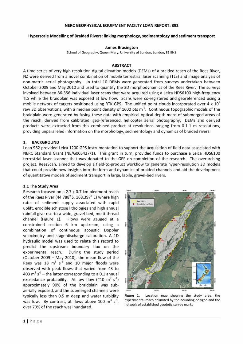
2. SURVEY METHODS A principal objective of the research was to develop a survey workflow capable of generating seamless, sub-metre fluvial morphological models at sufficient resolution and precision to detect subtle (10-2 – 10-1 m) topographic changes and derive roughness-based proxies for surface grain-size. Additionally, the methods used were required to cover a the 2.7 x 0.7 km reach, comprising both exposed and submerged topography, a complex network of channels, soft-sediments and where low flows between flood events could be restricted to only a few days. The solution identified was a hybrid terrestrial and aerial approach, that uses a fusion of mobile terrestrial laser scanning for exposed bar surfaces and image analysis of helicopter based aerial photography for submerged areas. The workflow is presented graphically in Figure 2 and the following sections describe the geodetic control network established to provide a common reference system for all surveys and the methods used during field data acquisition. The reader is directed to more comprehensive descriptions published elsewhere for further information (Brasington, 2010; Brasington et al., 2011; 2012; Rychkov et al., 2012; Williams et al. 2011; 2013a; 2013b).

Figure 2. Workflow for developing continuous hyperscale DEMs of braided rivers

2.1 Geodetic Control A framework for geodetic control in New Zealand is provided by PositionNZ, the Land Information New Zealand’s Global Positioning System Active Control Network. This network provides real-time and archived GPS carrier phase and code range measurements from 30 active stations to support GPS positioning

NERC Geophysical Equipment Facility - View more reports on our website at http://gef.nerc.ac.uk/reports.php

3 | P a g e

relative to New Zealand Geodetic Datum 2000 (NZGD2000). This network was used to establish a local monumented master survey mark [ORC BM] in a secure location 5 km from the reach. Static 1 Hz GPS observations acquired with a Leica GX1230 were recorded continuously for three ~8 hour intervals over consecutive days in October 2009. The position of [ORC BM] was obtained with reference to the closest active station (Mavora Lakes, [MAVL]) along a 60.8 km baseline using precise ephemeris data and processed using Leica GeoOffice 7.0. A network of eight survey marks were then established around the survey reach (see Figure 1) using [ORC BM] as the local reference station. Marks were installed in stable areas surrounding the active braidplain, using either 600 mm PERMA-MARKs or by setting marks in concrete, within stable, partially buried boulders. Positions were obtained using 2-4 hour static occupations, with the processed coordinates transformed into the NZ Tranverse Mercator coordinate system (NZTM2000) and orthometric heights determined in terms of the New Zealand Vertical Datum 2009 (NZVD2009) and the NZGeoid2009 surface. A full list of the permanent survey marks is given in Table 1.

Table 1. Survey marks established for the geodetic control network

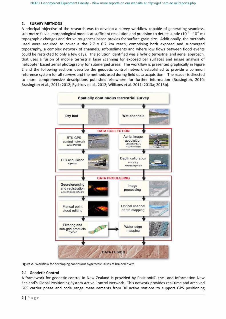
2.2 Dry Bed Survey: Terrestrial Laser Scanning Exposed riverbed topography was surveyed using the bespoke ArgoScan system. This incorporates: a gimbal supported Leica HDS61000 TLS; a 1200 GPS receiver; a panoramic camera; an onboard systems control PC with resilient data backup; battery charging facilities; all mounted on an Argo amphibious all-terrain vehicle capable of traversing the braidplain at low flows (Figure 3). A simultaneous localization and mapping (SLAM) routine, based on horizon tracking, was developed for ArgoScan to enable kinematic data capture, however, to ensure robust data quality, scans were acquired in rapid stop-and-go mode.

Figure 3. The ArgoScan system developed for rapid terrestrial survey over complex fluvial terrain.

The HDS6100 has an optimum range of 79 m, however the low albedo of the wet gravels combined with line of sight losses over the complex, shallow topography and low-angle view, resulted in ellipsoidal point clouds with dimensions of ~70 x 90 m in the transverse and streamwise directions. To ensure complete coverage and redundancy for quality assurance, scans were therefore acquired at intervals of 65 m in the cross-stream direction and 75 m streamwise. Scans were obtained with a 3D angular resolution of 0.018o, resulting in a point spacing of 7.9 mm at a range of 25 m. Each point cloud comprised between 10-15 million xyz observations with an acquisition time of ~3 minutes. Coverage of the entire reach involved between 287-351 individual scans, generating over 4 x 109 survey observations, although for some of the smaller floods, surveys were restricted to the active morphodynamic belt of the braidplain.

Construction of a unified point cloud requires registration and georeferencing of the individual scans, and this was achieved using a mobile network of RTK-GPS survey targets. For each scan, two tripod-mounted targets were deployed 10–15 m from the scanner at an angle of approximately 120o (Figure 4).

Survey Mark Date Placed Type Solution Frequencies Latitude Longitude Ell Ht Easting Northing Ortho Ht 3d Quality

(dms) (dms) (m) (m) (m) (m) (m)

ORC_BM 10/10/2009 Ref 44 51 13.308619 S 168 23 16.374696 E 324.292 1235568.359 5022945.381 315.628 0.007

RR_TL1 14/10/2009 Static Phase: fix all L1 + L2 44 47 25.642359 S 168 23 43.371847 E 340.792 1235762.082 5030004.224 332.037 0.001




RR_TR1 19/10/2009 Static Phase: fix all L1 + L2 44 47 21.856969 S 168 23 14.736625 E 342.943 1235126.232 5030085.297 334.199 0.000





4 | P a g e

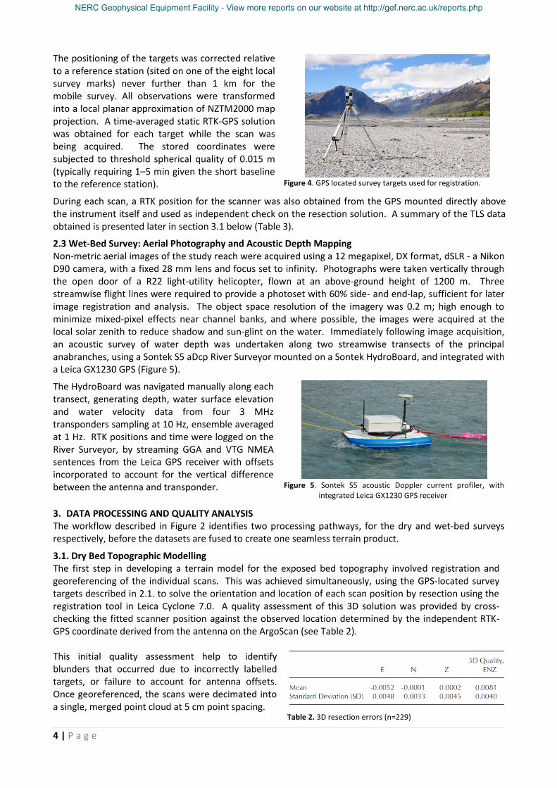
The positioning of the targets was corrected relative to a reference station (sited on one of the eight local survey marks) never further than 1 km for the mobile survey. All observations were transformed into a local planar approximation of NZTM2000 map projection. A time-averaged static RTK-GPS solution was obtained for each target while the scan was being acquired. The stored coordinates were subjected to threshold spherical quality of 0.015 m (typically requiring 1–5 min given the short baseline to the reference station).

Figure 4. GPS located survey targets used for registration.

During each scan, a RTK position for the scanner was also obtained from the GPS mounted directly above the instrument itself and used as independent check on the resection solution. A summary of the TLS data obtained is presented later in section 3.1 below (Table 3).

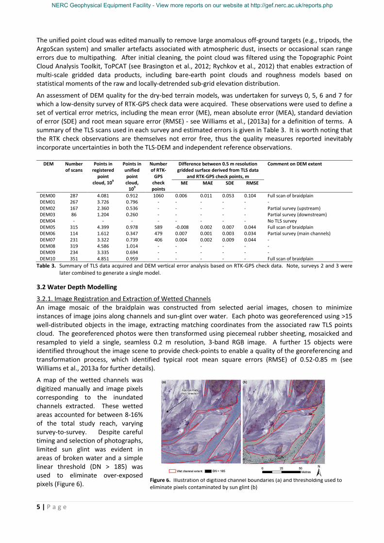
2.3 Wet-Bed Survey: Aerial Photography and Acoustic Depth Mapping Non-metric aerial images of the study reach were acquired using a 12 megapixel, DX format, dSLR - a Nikon D90 camera, with a fixed 28 mm lens and focus set to infinity. Photographs were taken vertically through the open door of a R22 light-utility helicopter, flown at an above-ground height of 1200 m. Three streamwise flight lines were required to provide a photoset with 60% side- and end-lap, sufficient for later image registration and analysis. The object space resolution of the imagery was 0.2 m; high enough to minimize mixed-pixel effects near channel banks, and where possible, the images were acquired at the local solar zenith to reduce shadow and sun-glint on the water. Immediately following image acquisition, an acoustic survey of water depth was undertaken along two streamwise transects of the principal anabranches, using a Sontek S5 aDcp River Surveyor mounted on a Sontek HydroBoard, and integrated with a Leica GX1230 GPS (Figure 5).

The HydroBoard was navigated manually along each transect, generating depth, water surface elevation and water velocity data from four 3 MHz transponders sampling at 10 Hz, ensemble averaged at 1 Hz. RTK positions and time were logged on the River Surveyor, by streaming GGA and VTG NMEA sentences from the Leica GPS receiver with offsets incorporated to account for the vertical difference between the antenna and transponder.

Figure 5. Sontek S5 acoustic Doppler current profiler, with

integrated Leica GX1230 GPS receiver

3. DATA PROCESSING AND QUALITY ANALYSIS The workflow described in Figure 2 identifies two processing pathways, for the dry and wet-bed surveys respectively, before the datasets are fused to create one seamless terrain product.

3.1. Dry Bed Topographic Modelling The first step in developing a terrain model for the exposed bed topography involved registration and georeferencing of the individual scans. This was achieved simultaneously, using the GPS-located survey targets described in 2.1. to solve the orientation and location of each scan position by resection using the registration tool in Leica Cyclone 7.0. A quality assessment of this 3D solution was provided by cross-checking the fitted scanner position against the observed location determined by the independent RTK-GPS coordinate derived from the antenna on the ArgoScan (see Table 2). This initial quality assessment help to identify blunders that occurred due to incorrectly labelled targets, or failure to account for antenna offsets. Once georeferenced, the scans were decimated into a single, merged point cloud at 5 cm point spacing.

Table 2. 3D resection errors (n=229)


5 | P a g e

The unified point cloud was edited manually to remove large anomalous off-ground targets (e.g., tripods, the ArgoScan system) and smaller artefacts associated with atmospheric dust, insects or occasional scan range errors due to multipathing. After initial cleaning, the point cloud was filtered using the Topographic Point Cloud Analysis Toolkit, ToPCAT (see Brasington et al., 2012; Rychkov et al., 2012) that enables extraction of multi-scale gridded data products, including bare-earth point clouds and roughness models based on statistical moments of the raw and locally-detrended sub-grid elevation distribution.

An assessment of DEM quality for the dry-bed terrain models, was undertaken for surveys 0, 5, 6 and 7 for which a low-density survey of RTK-GPS check data were acquired. These observations were used to define a set of vertical error metrics, including the mean error (ME), mean absolute error (MEA), standard deviation of error (SDE) and root mean square error (RMSE) - see Williams et al., (2013a) for a definition of terms. A summary of the TLS scans used in each survey and estimated errors is given in Table 3. It is worth noting that the RTK check observations are themselves not error free, thus the quality measures reported inevitably incorporate uncertainties in both the TLS-DEM and independent reference observations.

DEM Number of scans

Points in registered

point cloud, 109

Points in unified point cloud,

109

Number of RTK-

GPS check points

Difference between 0.5 m resolution gridded surface derived from TLS data

and RTK-GPS check points, m

Comment on DEM extent

ME MAE SDE RMSE

DEM00 287 4.081 0.912 1060 0.006 0.011 0.053 0.104 Full scan of braidplain DEM01 267 3.726 0.796 - - - - - - DEM02 167 2.360 0.536 - - - - - Partial survey (upstream) DEM03 86 1.204 0.260 - - - - - Partial survey (downstream) DEM04 - - - - - - - - No TLS survey DEM05 315 4.399 0.978 589 -0.008 0.002 0.007 0.044 Full scan of braidplain DEM06 114 1.612 0.347 479 0.007 0.001 0.003 0.034 Partial survey (main channels) DEM07 231 3.322 0.739 406 0.004 0.002 0.009 0.044 - DEM08 319 4.586 1.014 - - - - - - DEM09 234 3.335 0.694 - - - - - - DEM10 351 4.851 0.959 - - - - - Full scan of braidplain

Table 3. Summary of TLS data acquired and DEM vertical error analysis based on RTK-GPS check data. Note, surveys 2 and 3 were later combined to generate a single model.

3.2 Water Depth Modelling

3.2.1. Image Registration and Extraction of Wetted Channels An image mosaic of the braidplain was constructed from selected aerial images, chosen to minimize instances of image joins along channels and sun-glint over water. Each photo was georeferenced using >15 well-distributed objects in the image, extracting matching coordinates from the associated raw TLS points cloud. The georeferenced photos were then transformed using piecemeal rubber sheeting, mosaicked and resampled to yield a single, seamless 0.2 m resolution, 3-band RGB image. A further 15 objects were identified throughout the image scene to provide check-points to enable a quality of the georeferencing and transformation process, which identified typical root mean square errors (RMSE) of 0.52-0.85 m (see Williams et al., 2013a for further details).

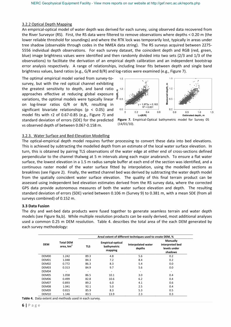
A map of the wetted channels was digitized manually and image pixels corresponding to the inundated channels extracted. These wetted areas accounted for between 8-16% of the total study reach, varying survey-to-survey. Despite careful timing and selection of photographs, limited sun glint was evident in areas of broken water and a simple linear threshold (DN > 185) was used to eliminate over-exposed pixels (Figure 6).

Figure 6. Illustration of digitized channel boundaries (a) and thresholding used to eliminate pixels contaminated by sun glint (b)


6 | P a g e

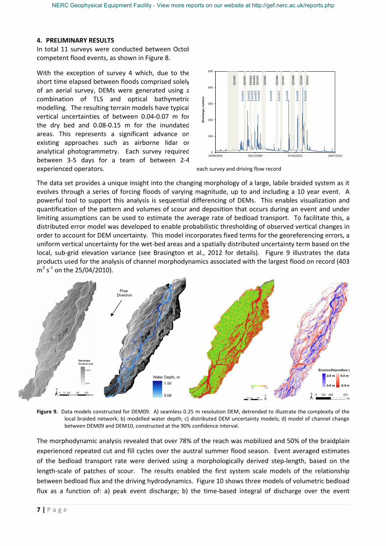
3.2.2 Optical Depth Mapping An empirical-optical model of water depth was derived for each survey, using observed data recovered from the River Surveyor (RS). First, the RS data were filtered to remove observations where depths < 0.20 m (the lower reliable threshold for soundings) and where the RTK lock was temporarily lost, typically in areas under tree shadow (observable through codes in the NMEA data string). The RS surveys acquired between 2275-5556 individual depth observations. For each survey dataset, the coincident depth and RGB (red, green, blue) image brightness values were identified and then randomly divided into two sets (2/3 and 1/3 of the observations) to facilitate the derivation of an empirical depth calibration and an independent bootstrap error analysis respectively. A range of relationships, including linear fits between depth and single band brightness values, band ratios (e.g., G/R and B/R) and log-ratios were examined (e.g., Figure 7).

The optimal empirical model varied from survey-to-survey, but with the red optical channel exhibiting the greatest sensitivity to depth, and band ratio approaches effective at reducing global exposure variations, the optimal models were typically linear on log-linear ratios G/R or B/R, resulting in significant bivariate relationships (p < 0.05) and model fits with r2 of 0.67-0.85 (e.g., Figure 7) and standard deviation of errors (SDE) for the predicted vs observed depth of between 0.067-0.158 m.

Figure 7. Empirical-Optical bathymetric model for Survey 05 (14/01/10).

3.2.3. Water Surface and Bed-Elevation Modelling The optical-empirical depth model requires further processing to convert these data into bed elevations. This is achieved by subtracting the modelled depth from an estimate of the local water surface elevation. In turn, this is obtained by pairing TLS observations of the water edge at either end of cross-sections defined perpendicular to the channel thalweg at 5 m intervals along each major anabranch. To ensure a flat water surface, the lowest elevation in a 1.5 m radius sample buffer at each end of the section was identified, and a continuous raster model of the water surface fitted by interpolation, using the modelled sections as breaklines (see Figure 2). Finally, the wetted channel bed was derived by subtracting the water depth model from the spatially coincident water surface elevation. The quality of this final terrain product can be assessed using independent bed elevation estimates derived from the RS survey data, where the corrected GPS data provide autonomous measures of both the water surface elevation and depth. The resulting standard deviation of errors (SDE) varied between 0.106 m (Survey 9) to 0.381 m, with a mean SDE (from all surveys combined) of 0.152 m.

3.3 Data Fusion The dry and wet-bed data products were fused together to generate seamless terrain and water depth models (see Figure 9a,b). While multiple resolution products can be easily derived, most additional analyses used a common 0.25 m DEM resolution. Table 4. describes the total area of the each DEM generated by each survey methodology:

DEM Total DEM area, km2

Areal extent of different techniques used to create DEM, %

TLS Empirical-optical

bathymetric mapping

Interpolated water depths

Manually interpreted bed

levels under shadows

DEM00 1.242 89.3 4.8 5.6 0.2 DEM01 1.048 84.3 7.2 8.4 0.2 DEM02 0.772 86.3 8.3 5.4 0.0 DEM03 0.313 84.9 9.7 5.6 0.0 DEM04 - - - - - DEM05 1.058 86.5 10.1 3.0 0.4 DEM06 0.499 82.8 10.6 6.2 0.4 DEM07 0.893 89.2 6.0 4.1 0.6 DEM08 1.041 92.1 5.0 2.5 0.4 DEM09 0.815 85.9 8.3 5.3 0.5 DEM10 1.146 83.5 13.9 2.3 0.3

Table 4. Data extent and methods used in each survey.


7 | P a g e

4. PRELIMINARY RESULTS In total 11 surveys were conducted between October 2009 and May 2010, before and after consecutive competent flood events, as shown in Figure 8.

With the exception of survey 4 which, due to the short time elapsed between floods comprised solely of an aerial survey, DEMs were generated using a combination of TLS and optical bathymetric modelling. The resulting terrain models have typical vertical uncertainties of between 0.04-0.07 m for the dry bed and 0.08-0.15 m for the inundated areas. This represents a significant advance on existing approaches such as airborne lidar or analytical photogrammetry. Each survey required between 3-5 days for a team of between 2-4 experienced operators.

Figure 8. Survey data acquisition schedule showing the timing of each survey and driving flow record

The data set provides a unique insight into the changing morphology of a large, labile braided system as it evolves through a series of forcing floods of varying magnitude, up to and including a 10 year event. A powerful tool to support this analysis is sequential differencing of DEMs. This enables visualization and quantification of the pattern and volumes of scour and deposition that occurs during an event and under limiting assumptions can be used to estimate the average rate of bedload transport. To facilitate this, a distributed error model was developed to enable probabilistic thresholding of observed vertical changes in order to account for DEM uncertainty. This model incorporates fixed terms for the georeferencing errors, a uniform vertical uncertainty for the wet-bed areas and a spatially distributed uncertainty term based on the local, sub-grid elevation variance (see Brasington et al., 2012 for details). Figure 9 illustrates the data products used for the analysis of channel morphodynamics associated with the largest flood on record (403 m3 s-1 on the 25/04/2010).

Figure 9. Data models constructed for DEM09. A) seamless 0.25 m resolution DEM, detrended to illustrate the complexity of the local braided network; b) modelled water depth; c) distributed DEM uncertainty models; d) model of channel change between DEM09 and DEM10, constructed at the 90% confidence interval.

The morphodynamic analysis revealed that over 78% of the reach was mobilized and 50% of the braidplain

experienced repeated cut and fill cycles over the austral summer flood season. Event averaged estimates

of the bedload transport rate were derived using a morphologically derived step-length, based on the

length-scale of patches of scour. The results enabled the first system scale models of the relationship

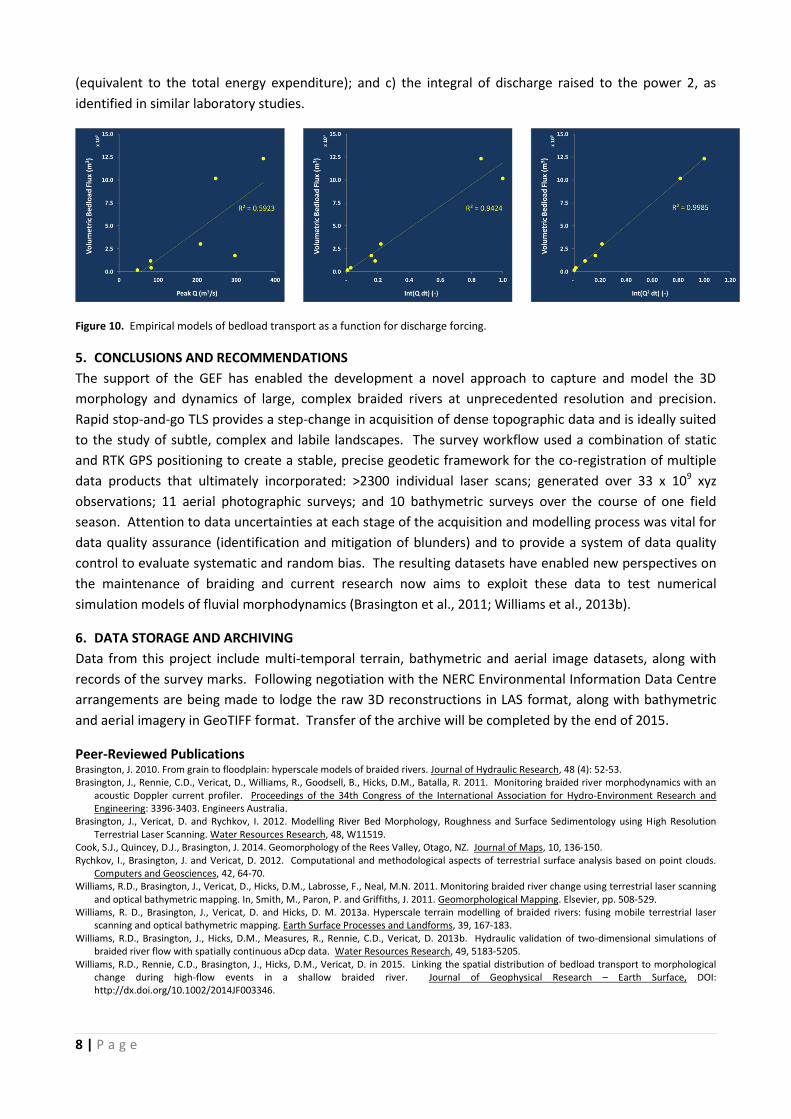
between bedload flux and the driving hydrodynamics. Figure 10 shows three models of volumetric bedload

flux as a function of: a) peak event discharge; b) the time-based integral of discharge over the event

0

100

200

300

400

500

19/09/2009 28/12/2009 07/04/2010 16/07/2010

Dis

ch

arg

e, cu

mecs

DE

M00

Event0

2

Event0

3

Event0

4

Event0

1

DE

M10

DE

M09

DE

M08

DE

M07

DE

M06

DE

M05

DE

M02

DE

M03

DE

M04

DE

M01

Event0

5

Event0

6

Event0

7

Event0

8

Event0

9

Event1

0


8 | P a g e

(equivalent to the total energy expenditure); and c) the integral of discharge raised to the power 2, as

identified in similar laboratory studies.

Figure 10. Empirical models of bedload transport as a function for discharge forcing.

5. CONCLUSIONS AND RECOMMENDATIONS

The support of the GEF has enabled the development a novel approach to capture and model the 3D

morphology and dynamics of large, complex braided rivers at unprecedented resolution and precision.

Rapid stop-and-go TLS provides a step-change in acquisition of dense topographic data and is ideally suited

to the study of subtle, complex and labile landscapes. The survey workflow used a combination of static

and RTK GPS positioning to create a stable, precise geodetic framework for the co-registration of multiple

data products that ultimately incorporated: >2300 individual laser scans; generated over 33 x 109 xyz

observations; 11 aerial photographic surveys; and 10 bathymetric surveys over the course of one field

season. Attention to data uncertainties at each stage of the acquisition and modelling process was vital for

data quality assurance (identification and mitigation of blunders) and to provide a system of data quality

control to evaluate systematic and random bias. The resulting datasets have enabled new perspectives on

the maintenance of braiding and current research now aims to exploit these data to test numerical

simulation models of fluvial morphodynamics (Brasington et al., 2011; Williams et al., 2013b).

6. DATA STORAGE AND ARCHIVING

Data from this project include multi-temporal terrain, bathymetric and aerial image datasets, along with

records of the survey marks. Following negotiation with the NERC Environmental Information Data Centre

arrangements are being made to lodge the raw 3D reconstructions in LAS format, along with bathymetric

and aerial imagery in GeoTIFF format. Transfer of the archive will be completed by the end of 2015.

Peer-Reviewed Publications Brasington, J. 2010. From grain to floodplain: hyperscale models of braided rivers. Journal of Hydraulic Research, 48 (4): 52-53. Brasington, J., Rennie, C.D., Vericat, D., Williams, R., Goodsell, B., Hicks, D.M., Batalla, R. 2011. Monitoring braided river morphodynamics with an

acoustic Doppler current profiler. Proceedings of the 34th Congress of the International Association for Hydro-Environment Research and Engineering: 3396-3403. Engineers Australia.

Brasington, J., Vericat, D. and Rychkov, I. 2012. Modelling River Bed Morphology, Roughness and Surface Sedimentology using High Resolution Terrestrial Laser Scanning. Water Resources Research, 48, W11519.

Cook, S.J., Quincey, D.J., Brasington, J. 2014. Geomorphology of the Rees Valley, Otago, NZ. Journal of Maps, 10, 136-150. Rychkov, I., Brasington, J. and Vericat, D. 2012. Computational and methodological aspects of terrestrial surface analysis based on point clouds.

Computers and Geosciences, 42, 64-70. Williams, R.D., Brasington, J., Vericat, D., Hicks, D.M., Labrosse, F., Neal, M.N. 2011. Monitoring braided river change using terrestrial laser scanning

and optical bathymetric mapping. In, Smith, M., Paron, P. and Griffiths, J. 2011. Geomorphological Mapping. Elsevier, pp. 508-529. Williams, R. D., Brasington, J., Vericat, D. and Hicks, D. M. 2013a. Hyperscale terrain modelling of braided rivers: fusing mobile terrestrial laser

scanning and optical bathymetric mapping. Earth Surface Processes and Landforms, 39, 167-183. Williams, R.D., Brasington, J., Hicks, D.M., Measures, R., Rennie, C.D., Vericat, D. 2013b. Hydraulic validation of two-dimensional simulations of

braided river flow with spatially continuous aDcp data. Water Resources Research, 49, 5183-5205. Williams, R.D., Rennie, C.D., Brasington, J., Hicks, D.M., Vericat, D. in 2015. Linking the spatial distribution of bedload transport to morphological

change during high-flow events in a shallow braided river. Journal of Geophysical Research – Earth Surface, DOI: http://dx.doi.org/10.1002/2014JF003346.

Documents

Hyperscale Modelling of Braided Rivers: linking morphology ...gef.nerc.ac.uk/documents/report/892.pdf · 1 | P a g e NERC GEOPHYSICAL EQUIPMENT FACILTY LOAN REPORT: 892 Hyperscale