Embed Size (px)
Citation preview
Berit Time
Hygroscopic Moisture Transport in Wood
A thesis presented for the degree of Doktor Ingeniør of the
Norwegian University of Science and Technology Department of Building and Construction Engineering
February 1998
iii
Summary Spruce together with pine are the main wooden building materials used in Norway. Due to the complex composition of the material and the many-sided usage, there still are many un-answered questions concerning moisture transport in wood in buildings. Wood and wooden materials in buildings are exposed to diurnal and annual climatic cycles. Uncertainties concerning transient wood-water relations in buildings and building components have demanded a more thorough investigation on basic moisture transport in wood and related properties. This thesis is a result of a comprehensive study on hygroscopic moisture transport in wood in general and spruce (Picea abies) in particular. The themes focused in this thesis can be divided into three parts. In the first part, a thorough study of present knowledge of moisture sorption and moisture transport in wood have been conducted. Material properties have also been measured and investigated in this part. It has been shown that diffusion coefficients, Dp, determined from cup measurements are increasing with an increasing average relative humidity across a wooden specimen. It has also been confirmed that if diffusion coefficients, DC, determined from transient sorption measurements are to be converted to Dp , significant variations in diffusion coefficients can be obtained depending on the parameters included in the conversion factor. Absorption and desorption isotherms of spruce (Picea abies) measured in this work have been compared with corresponding measurements on spruce performed in other Nordic countries, and significant deviations have been found. In the second and main part of this thesis, experimental investigations on wood exposed to cyclic step-changes in climatic conditions have been performed. Two different sets of experiments have been performed. In the main set of experiments an experimental apparatus has been designed and set up in the laboratory at the department. Well known principles for measurement of moisture sorption in wood have been employed. As there is a demand for less labour intensive and more efficient methods for measuring moisture sorption in wood, another set of experiments has been conducted in the laboratory at Department of Chemical and Process Engineering (CAPE), University of Canterbury, New Zealand. In these experiments another, more efficient, principle of measurement, originally meant for drying experiments, has been employed and assessed for measuring moisture sorption in wood.
iv
The results from four different measurement series, conducted at the department, with diurnal and weekly cycles between two different levels have been reported. A two-step sorption process has been observed with the major change in moisture content in the first fast initial part. No significant phase lag has been observed for neither transverse nor longitudinal specimens up to 10 mm thickness. A repetitive pattern in moisture content change is found for both weekly and daily changes. The same level of moisture content is reached in both absorption and desorption every cycle. Although average moisture contents have been measured only, the fast response in moisture sorption indicates that significant moisture gradients are present immediately after a relatively large change in surrounding humidity. The results from four different sorption experiments, conducted at CAPE, have indicated the presence of the same two-step sorption process, with the major change in moisture content within the first fast initial part of sorption. The specimens in these experiments were exposed to time gradients in both temperature and relative humidity. The overall impression from these experiments is that the apparent «equilibrium» moisture contents are rather high for all temperature and humidity levels. The reason for this has not been possible to fully explain. However, weaknesses in the principle of measurement have been revealed. In the third part of this thesis, a one-dimensional transient model for moisture transport in wood is set up. The model is based on Fick’s law with water vapour pressure and temperature as driving potentials. A model for hysteresis has been proposed and included in the model. Comparisons between the experimental results obtained in this work and calculations have been done. The level of the absorption and the desorption isotherm is the most important parameter in order to obtain good fit between measurements and calculations. A better agreement is found if hysteresis is taken into account, compared to calculations where only an average sorption isotherm is used. It is also found that the diffusion coefficient and its dependency on RH and the density of the wood have a certain influence on the sorption rate. The convection mass transfer coefficient on the other side has very little influence on the average moisture content. As an approach to modelling moisture transport in wood exposed to cyclic environmental changes in the hygroscopic range, the model has proved promising. The shape of the measured and the calculated curves presented in this work correspond very well. This could imply that application of linear intermediate curves, based on empirical data, could be a suitable way of modelling hysteresis in wood.
v
Preface The work presented in this report has been made possible by financial support from the Research Council of Norway through the research programme «Moisture in Building Materials and Constructions». Financial support in association with this work has also been received from NTH foundation and A/S Veidekke. The work has been carried out as a thesis presented for the degree of Doktor Ingeniør at Department of Building and Construction Engineering, The Norwegian University of Technology. I would like to thank Professor Jan Vincent Thue for being my supervisor and for being open for discussions at any time. He has given me the feeling of «security» in my work by his strong knowledge and skill. I also want to thank my former colleagues and fellow graduate students at Department of Building and Construction Engineering for guidance, discussions and social events. Hans Boye Skogstad and former graduate student Hege Furuseth in particular for assistance with the experiments. At the Faculty of Civil and Environmental Engineering: many thanks to the technicians at the workshop for their help in building the experimental equipment and to Eirik Fyhn, for helping with the drawings presented in this report. I would like to thank colleagues at the Norwegian Building Research Institute, Trondheim Division, for assistance, support and good company throughout these years. Einar Bergheim in particular for assistance with the experiments, Doktor ingeniør Tom-Nils Nilsen for answering my many questions concerning chemistry, Annanias Tveit, now retired from his research position, for his advices and finally the leadership of the institute for offering me a position. I am grateful to Professor Emeritus Roger B. Keey and the staff at the Department of Chemical and Process Engineering, University of Canterbury, Christchurch, New Zealand, for their guidance and hospitality during my stay at the department from September 1996 to February 1997. Finally, not least, thanks to Mona, Kirsti and Lisbet for moral support and sharing of fate, Jakob and Tom for being pleasures of life.
Trondheim, February 1998 Berit Time

vi

Contents Summary iii Preface v Contents vii Nomenclature xi Themes xiii Chapter 1 Introduction to the Wooden Material 1 1.1 The wood structure 1 1.2 The wood cell wall 4 1.3 Density of wood 6 1.4 Shrinkage and swelling of wood 6 1.5 Deformations, stresses and strains in wood 7 1.6 Wood, a building material 8 Chapter 2 Sorption in Wood 9 2.1 Background 9 2.2 The physical and chemical nature of sorption 11 2.3 Sorption theories 16 2.4 Hysteresis 28 2.5 Intermediate curves 33 2.6 Sorption isotherms and temperature dependence 35 2.7 Sorption isotherm measurements on spruce (Picea abies) performed in the Nordic countries 38 2.8 Sorption in wood related to building physics and - engineering practice 43 Chapter 3 Moisture Transport in Wood - Theory and Experiences 47 3.1 Moisture transport mechanisms 47 3.2 Isothermal diffusion equations 52 3.3 Non-isothermal moisture movement 55
Contents
viii
Chapter 4 Diffusion Coefficients 63 4.1 Methods for evaluation of diffusion coefficients 63 4.2 Diffusion coefficients evaluated from sorption measurements 65 4.3 Diffusion measurements of spruce by the cup method 69 4.4 Comparison of diffusion coefficients obtained by the two methods 80 4.5 Conversion of diffusion coefficients 82 Chapter 5 Sorption Measurements of Spruce Exposed to Cyclic Step Changes in Relative Humidity 91 5.1 Present knowledge 91 5.2 Experimental set-up 93 5.3 Results from measurements 98 5.4 Variations within the measuring series 107 5.5 Influence of surface area on moisture sorption 108 5.6 Hysteresis and slow sorption 109 5.7 Conclusions 118 Appendix 5.A: Measured climatic data and experiences 119 Chapter 6 Modelling of Transient Moisture Transport and Hysteresis in Wood 123 6.1 Introduction 123 6.2 Theory 125 6.3 Numerical solution method 128 6.4 Modelling of material properties 128 6.5 Hysteresis 132 6.6 Comparison of calculations and experimental results 136 6.7 Conclusions 146 Chapter 7 Use of a Modified Timber Drying Apparatus for Sorption in Spruce Part 1 - Experiments 149 7.1 Introduction 149 7.2 Description of the small timber drying chamber 150 7.3 Sorption Measurements in the SDC 168 7.4 Concluding discussion 179
ix
Chapter 8 Use of a Modified Timber Drying Apparatus for Sorption in Spruce Part 1 - Calculations 183 8.1 Introduction 183 8.2 Comparison between experimental results and calculations 184 8.3 Concluding discussion 195 Chapter 9 Conclusions 199 9.1 Main conclusions 199 9.2 Recommendations for further work 202 References 205

Contents
x

xi
Text
xi
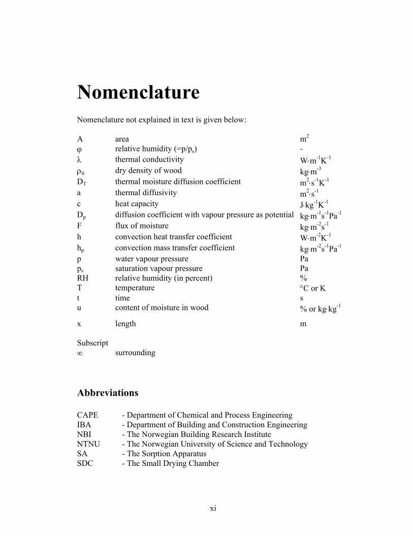
Nomenclature Nomenclature not explained in text is given below: A area m2 ϕ relative humidity (=p/ps) - λ thermal conductivity W⋅m-1K-1
ρ0 dry density of wood kg⋅m-3 DT thermal moisture diffusion coefficient m2⋅s-1K-1
a thermal diffusivity m2⋅s-1
c heat capacity J⋅kg-1K-1
Dp diffusion coefficient with vapour pressure as potential kg⋅m-1s-1Pa-1
F flux of moisture kg⋅m-2s-1 h convection heat transfer coefficient W⋅m-2K-1
hp convection mass transfer coefficient kg⋅m-2s-1Pa-1 p water vapour pressure Pa ps saturation vapour pressure Pa RH relative humidity (in percent) % T temperature °C or K t time s u content of moisture in wood % or kg⋅kg-1
x length m Subscript ∞ surrounding Abbreviations CAPE - Department of Chemical and Process Engineering IBA - Department of Building and Construction Engineering NBI - The Norwegian Building Research Institute NTNU - The Norwegian University of Science and Technology SA - The Sorption Apparatus SDC - The Small Drying Chamber

Nomenclature
xii
RH - Relative humidity (%) rh - Relative humidity (-) MC - Moisture content FSP - Fibre saturation point EMC - Equilibrium moisture content
xiii
Themes This thesis presents a comprehensive study on moisture transport in wood. It consists of an introduction to wood as a material (Chapter 1) and seven separate chapters (Chapter 2 - 8) concerning different issues related to moisture transport in wood in general and spruce in particular. Results from experiments performed in this work can be found in Chapter 2, 4, 5 and 7. Results from modelling and calculations performed in this work can be found in Chapter 6 and 8. Background Wood and wood based materials are among the most important building materials in Norway. Wood is an organic material with a very complex composition. Due to its complex composition and its many-sided usage there still are many un-answered questions concerning wood in use in buildings. In buildings wood is subjected to shrinkage, swelling, mould growth and rot if exposed to unfavourable environmental conditions. These phenomena are all related to moisture content and moisture conditions in a building structure. Rot may occur in wood which is in contact with liquid water for some time, while shrinkage, swelling and mould growth are mainly related to hygroscopic moisture, i.e., water vapour. Wood and wooden materials in buildings are exposed to smaller or larger changes in climate continuously. Outdoor climate changes are present throughout the day and night, and throughout the year. Indoor climate changes are more or less a result of the outdoor changes in addition to changes related to the inhabitants activities. There still is a need for improving and developing the basic knowledge of moisture in wood subjected to changing climatic conditions. There are several and different approaches to the topic. Several large scale experiments on building envelopes (e.g., walls and roofs) in order to investigate the heat, air and moisture performance have revealed that a more thorough investigation on basic moisture transport in wood is necessary. Poor agreement has been reported between accepted numerical models and measurements of moisture content in wooden materials in structures (Geving and Thue 1996). More recently recognised potential health hazards of mould and other organisms which flourish in buildings demand basic knowledge about moisture transport in wood.
Themes
xiv
In the sixties it was shown (Christensen 1965, Kelly and Hart 1970, Skaar et al. 1970) that the rate of moisture sorption to equilibrium is dependent on the level of the surrounding relative humidity and the size of the increase or decrease in relative humidity. A fast sorption rate was found for situations with the basis in a relatively low relative humidity and a fairly large increment. A much slower sorption rate was found for higher relative humidities and small increments. However, a two-step sorption rate was revealed for most situations. The first and immediate sorption is fast, and according to traditional diffusion theory, the second rate of sorption is of a much more slow character. More recent research has confirmed what was reported in the sixties (Wadsø 1993, Håkansson 1994, 1995a). It has also been found that different methods for measuring diffusion coefficients for wood give different results (Comstock 1963, Wadsø 1993). This has partly been explained by the observed differences in rate of sorption. Also in the field of conservation there has been revealed a need for a better knowledge of moisture sorption and moisture gradients in wood related to a fluctuating climate within buildings. Cracking of painted wooden art in Norwegian stave churches, due to climatic changes, is another occurrence which has demanded a more thorough study on moisture in wood. The stave churches are heated regularly to meet the comfort-need of the visiting people, something which has resulted in significant moisture gradients and cracking of the interior surfaces. For wood in buildings, moisture sorption to an equilibrium situation is rather rare. Moisture sorption in wood exposed to more rapid changes in climate is a more appearing situation. The aim of this thesis has been to investigate the moisture sorption of wood when pieces of wood are exposed to rapid changes in surrounding climate. The effect of the slow sorption in wood in such situations has also been investigated. Introduction to the thesis In Norway, there has been a need for improvement and development of knowledge concerning moisture in buildings, and a national research programme was set up in 1993. The work in this thesis is carried out as a research project within the research programme «Moisture in Building Materials and
xv
Constructions». Hygroscopic moisture transport in wood was one particular topic that was selected to emphasize. A thorough investigation has been done in order to map existing knowledge within the field of moisture sorption, moisture transport and transport properties of wood in general and spruce in particular. The main emphasis of the work has been in the area of experimental investigations. An effort has been put in designing and setting up experimental equipment in the laboratory of the department in order to facilitate experiments on wood exposed to cyclic changes in climatic conditions. Similar experiments, with the basis in another principle of measurement, have been performed by the author in a laboratory at the Department of Chemical and Process Engineering at Canterbury University, New Zealand. The results from the experimental investigations have been analysed and discussed, and the two different principle of measure moisture sorption have been compared. A numerical model for transient moisture transport in wood has been set up in order to facilitate comparison between measurements and calculations. Most of the necessary input parameters, i.e. climatic conditions (temperature and relative humidity), diffusion coefficients, sorption isotherms and density have been measured in this project. Additional parameters have been selected from the literature. A model for hysteresis has been proposed and included in the numerical model to render a study of the effect of hysteresis. The influence and the importance of the earlier observed and described slow sorption in wood, have been investigated and analysed in situations when wood is exposed to more rapid climatic changes. The way of studying moisture sorption is different for the society of wood science and the society of building physics. In building physics the main interested is in regarding wood as a part of a whole structure in a macroscopic perspective. Material properties should be achieved in a form that is appropriate for most building materials and for the building structure as a whole. Within wood science, however, wood and its complex structure in a more microscopic perspective are of main interest, and no regards in sense of other materials have to be taken. One aim of this thesis has been to regard moisture transport in a «building physics perspective» by benefiting from knowledge acquired within the society of wood science.

Themes
xvi
The physical structure of this thesis is: In Chapter 1 is given a brief introduction to the wooden material. Aspects concerning the structure and properties related to moisture are presented. In Chapter 2 is given an introduction and a review of past and present research on moisture sorption in wood. The physical and chemical background of the phenomenon is given. The most widely used models are presented and explained. The phenomenon of hysteresis is introduced and discussed. Experimental results of sorption isotherms of spruce are presented. In Chapter 3 is given a presentation of a theoretical background of hygroscopic moisture transport in wood. Different approaches for describing isothermal, non-isothermal, steady-state and transient moisture transport processes are presented. Results from measurements of diffusion coefficients are presented in Chapter 4. A thorough assessment of aspects concerning determination of diffusion coefficients is given. Chapter 5 deals with the experiments performed on moisture sorption of spruce exposed to step-changes in climatic conditions. The experimental equipment has been designed and built for this purpose. A brief description of the equipment is given. The results from the experimental investigations are thoroughly analysed. In Chapter 6 is presented a model for transient moisture transport in wood. A model for hysteresis is included. Calculations are performed and compared with the measured results obtained in Chapter 5. In Chapter 7 is presented results and evaluation of sorption measurements on spruce exposed to step-changes in surrounding climate using another principle of measurement. Finally, Chapter 8 contains calculations associated with the measurements presented in Chapter 7. In Chapter 9 is given overall conclusions and recommendations for further work. Limitations This thesis is concerned with hygroscopic (i.e., water vapour) moisture transport in wood and does not include liquid transport.

Chapter 1
Introduction to the Wooden Material This thesis deals with softwoods in general and spruce (Picea abies) in particular. Picea abies is also known as Norway spruce or European spruce. This type of spruce is mainly found in Europe (from the north of the Scandinavian countries, south to the Pyrenees and the Alps and towards east to the Ural mountains) (Stemsrud 1989). Spruce together with pine are the main wooden building materials used in Norway. It is used as exterior cladding, as structural parts as well as interior linings and floors. The structure and properties of wood are treated in a number of references. Where no references are given, the text in this chapter is based on general textbooks (Kollmann and Côté 1968, Siau 1984, Stemsrud 1989 and NTI 1991).
1.1 The wood structure The physical properties as well as the behaviour of wooden materials are highly dependent upon the structure of wood. It is therefore important to have an understanding of the essentials of this structure. Wood is an anisotropic and non-
2 Chapter1
homogeneous material. Wood comes from tree species which are divided into two main groups, namely softwood (or conifer) and hardwood (or dicotyledonous angiosperms). These two groups can be separated by their different characteristics, needles and leaves. All parts of the tree are composed of cells of different types and sizes. Cells which are formed by divisions in the cambium, which is a layer of living cells between the wood and the bark. The tree grows by adding new cells to the outside of the wood. Softwoods are much more uniform than hardwoods. The major part (90 - 95 %) of a softwood tree is made up of a type of long, hollow, tubular fibres (called tracheids), which are mainly vertical. Their length usually ranges from about 2.5 to 7 mm and their width is about one hundredth of the length (Mårtensson 1992). They give strength to the tree and serve as ducts for the transport of water all the way through the tree. Fibres which serve as a pathway for water transport are part of the sapwood of the softwood tree. Fibres which are cut off from the water transport make the heartwood of the tree. For some species such as pine the heartwood is darker than the sapwood. For spruce there is no visible difference between heartwood and sapwood in service. There are differences between sapwood and heartwood though. The heartwood has for instance a lower moisture content than the sapwood because it has been cut off from the water transport. In some cases the heartwood is more resistant to fungal attacks, and it can be more water repellent. When studying wood from a macro-structure point of view, the most striking feature is the growth rings. They contain fibres (tracheids) of two kinds, earlywood and latewood fibres. The earlywood fibres are formed in spring when the tree starts to grow after the winter. Their main task is to transport water and nutrient salts from the root to the leaves. They are thin walled with large lumens (cell cavities). The latewood fibres, which have a darker colour, are formed during summer when the tree has time to consolidate itself . They are thick walled, with small lumens and they are important for the strength of the tree. Water is transported from one fibre to another through intertracheid bordered pit pairs. These pit pairs are circular openings in adjacent cell walls, spanned by a thin membrane which is a continuation of the compound middle lamella, the cementing structure between fibres, see figure 1.2 (Mårtensson 1992). Most of these pit pairs are located on the radial surface of the fibres as can be seen on

Introduction to the Wooden Material 3
figure 1.1. There are smaller and fewer pits in latewood fibres than in earlywood and generally fewer pits of smaller size on the tangential surfaces. Stemsrud (1989) refers that in an earlywood fibre between 100 and 300 pit pairs can be found and in a latewood fibre only 10 to 15.
������������ ���������������
�
�
�����
Figure 1.1: Radial and tangential surfaces of fibres (tracheids). The size and the amounts of bordered pits can be seen. (t = tracheid, rbp = radial bordered pit, tbp = tangential bordered pit, rd = resin duct) Most softwoods also contain some resin ducts which are continuos tubes mainly extending in the longitudinal direction. Resin ducts are, in general, ineffective for movement of liquids or gases over any appreciable distance, despite the fact that they are continuous. This is because they are almost always clogged with resin. Wood always has knots and other deviations from the regular growth ring pattern. The amount of knots and other deviations depend on the growth area, the site class, genetic factors and the quality of the material. The different directions in a piece of wood are called longitudinal (L), tangential (T), radial (R ) or transversal or across the fibres (TR). The transversal direction very often shows the same properties as the tangential and the radial. For wood used in buildings the longitudinal and transversal are the most convenient directions to use. A beam or a board is never cut so that the water vapour transport can be regarded as merely tangential or radial.

4 Chapter1
1.2 The wood cell wall
1.2.1 Molecular structure The wood cell wall consists of three major polymer components: cellulose which is the skeleton, hemicellulose which is the matrix and lignin the encrusting substance which binds the cells together and gives rigidity to the cell wall. In addition, wood contains extractives. 40 - 50 % of the timber weight is cellulose, 20 - 30 % is hemicellulose, 25 - 30 % is lignin and 0 - 10 % is extractives (e.g. resin ). Cellulose: Cellulose is a major part of all plant materials and the most occurring polymer on earth. Wherever it occurs in nature it takes the form of long strands composed of cellulose molecules arranged more or less parallel to each other. In wood these are called microfibrils. When the cellulose chains are ordered evenly, with respect to each other in some parts of the microfibril, it is called crystalline cellulose. When the cellulose chains are not evenly ordered it is called amorphous cellulose. The crystallinity of wood cellulose is approximately 50 % (Wadsø 1993). The amorphous cellulose is hygroscopic while the crystalline is not. This gives the different parts of the cellulose different moisture properties. When water enters between the cellulose chains in the S2 layer, see figure 1.2, it forces the chains apart. This causes transverse (radial and tangential) swelling, while any change in the longitudinal direction is minor. The average amount of cellulose is relatively constant for wood of the same type (Stemsrud 1989). Hemicellulose: Similar to cellulose, hemicellulose is polysaccharides, but they are built from different kinds of sugar units. Hemicellulose has about the same hygroscopicity as amorphous cellulose. The property of the wood seems, to a certain degree, to be related to the amount of hemicellulose present. High density seems to be correlated to a low amount of hemicellulose. The content of hemicellulose seems to be relatively small in wood with thin cell walls. Lignin: Lignin is chemically dissimilar to both cellulose and hemicellulose. It is a polymer of phenyl groups and it consists of large amorphous molecules. Lignin in the cell wall gives stiffness to the cell wall and resistance to chemical degradation. Lignin is mainly found in the middle lamella between the microfibrils and the amount of lignin decreases towards the cell lumen. There is a difference in
Introduction to the Wooden Material 5
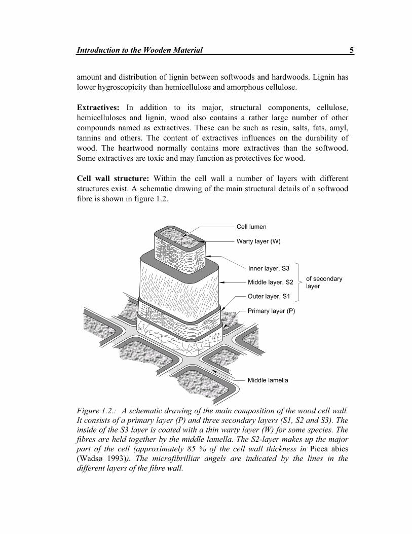
amount and distribution of lignin between softwoods and hardwoods. Lignin has lower hygroscopicity than hemicellulose and amorphous cellulose. Extractives: In addition to its major, structural components, cellulose, hemicelluloses and lignin, wood also contains a rather large number of other compounds named as extractives. These can be such as resin, salts, fats, amyl, tannins and others. The content of extractives influences on the durability of wood. The heartwood normally contains more extractives than the softwood. Some extractives are toxic and may function as protectives for wood. Cell wall structure: Within the cell wall a number of layers with different structures exist. A schematic drawing of the main structural details of a softwood fibre is shown in figure 1.2.
��������������
����������
�������������
���������������
�������������
����������� �
��������������
!�����������"
Figure 1.2.: A schematic drawing of the main composition of the wood cell wall. It consists of a primary layer (P) and three secondary layers (S1, S2 and S3). The inside of the S3 layer is coated with a thin warty layer (W) for some species. The fibres are held together by the middle lamella. The S2-layer makes up the major part of the cell (approximately 85 % of the cell wall thickness in Picea abies (Wadsø 1993)). The microfibrilliar angels are indicated by the lines in the different layers of the fibre wall.

6 Chapter1
1.3 Density of wood The density of wood is defined as the relationship between the mass and the volume of the specimen. As the cell wall of nearly all kinds of wood has the same density, approximately 1500 kg⋅m-3, it is the relationship between the amount of cell wall and cell lumen which gives the density of the wood. Wood is a hygroscopic material which changes mass and volume depending on the surrounding relative humidity. The density is dependent on the moisture content in the material. This means that it is of great necessity to define for which moisture conditions the actual density has been decided. In this thesis the dry density of the wooden specimens has been given. The density has been measured after the test specimens have been dried in an oven at 105°C or 70°C until no weight change is longer seen. The dry density of spruce (Picea abies) varies between 300 - 640 kg⋅m-3. The growth rate is of great influence to the density. Increasing annual ring width gives lower density.
1.4 Shrinkage and swelling of wood Wood undergoes dimensional changes following variations in moisture content and/or temperature. These changes are bigger in the case of changes in moisture content than in the case of changes in temperature. Within the cell wall the moisture is hydrogen bonded to the matrix components, mainly to the hemicellulose and to the hydroxyl groups of cellulose in the amorphous regions. When the moisture evaporates from the cell wall, the matrix shrinks and the microfibrils come closer together. In the direction of the microfibril (i.e. longitudinal direction) there is very little change in dimension. This is mainly because the fibre cell walls are so much more apart in the longitudinal direction (approximately 100 cell walls in the transverse direction to one in the longitudinal for the same distance).

Introduction to the Wooden Material 7
The shrinkage and swelling behaviour depends on tree species and where in the tree the measurement is made. There is a significant difference between normal wood and compression wood for instance. For all types of wood, the shrinkage and swelling behaviour differs between the three main directions. In (NTI 1991) the total shrinkage values, i.e. from approximately fibre saturation, 30 weight %, to 0 weight %, are given for spruce (Picea abies). These are 0.3 % in the longitudinal direction, 3.6 % in the radial direction and 7.8 % in the tangential direction. The difference between tangential and radial shrinkage-swelling is not fully explained (Mårtensson 1992). Several reasonable explanations for the shrinkage-swelling anisotropy between tangential and radial direction have been proposed, but none of them actually proved. The most commonly used explanation is the occurrence of wood rays in the radial direction. The existence of wood rays is supposed to have a restraining effect on the shrinkage in the radial direction. The effect is found to be more pronounced for hardwoods than for softwoods. However, a significant difference between radial and tangential shrinkage-swelling can still be found even though no rays are present. Another theory is based on the difference in shrinkage between earlywood and latewood. A third theory suggests that the poorer orientation of the microfibrils in the radial walls, as compared to the tangential walls, can account for the difference in shrinkage. And at last it has been shown that the degree of lignification is higher in the radial walls than in the tangential, something which could explain some of the anisotropy in shrinkage-swelling. None of the theories mentioned above have ever been proved, but all of them are likely to be of relevance for the radial and tangential shrinkage-swelling behaviours.
1.5 Deformations, stresses and strains in wood Deformations and volumetric changes are found in wood in many situations. Such situations may be; during growth, during drying (seasoning), during loading and unloading and in service due to climatic changes (changes in relative humidity and temperature) and load. Due to the growing process wood is never in a total stress-free state (Mårtensson 1992). Growth stresses are normally dealt with isolated. Growth stresses in timber
8 Chapter1
have been defined by the Society of American Foresters as the forces found in green woody stems. They are thus segregated from the stresses and strains occurring in timber as a result of the removal of water due to e.g. seasoning (Nilsson 1993). In a wooden specimen under load there is an initial elastic strain, εi , in response to the load applied to the specimen. If the test specimen is thereafter kept under constant load and constant climatic conditions the strain increases with time and pure creep, εc, occurs. If the test specimen is instead subjected to humidity changes, the total strain oscillates due to the moisture changes and mechano-sorptive strains, εms, occur. In addition to the above mentioned strains, the total strain also include the free-shrinkage strain caused by reduction of the moisture content below the fibre saturation point (FSP), εS0, and strain due to temperature changes, εT. Mechano-sorptive deformations, or often called mechano-sorptive effects, were first investigated in the late fifties and early sixties. It was first not distinguished from creep strains (Carrington 1996). In some cases the two different components of strain are still combined and called mechano-sorptive creep strain and different definitions exist.
1.6 Wood, a building material
To sum up; wood is a natural material with a very complex composition. The properties differ from species to species, from tree to tree and also within the different parts of a tree. In older days when woodwork in buildings was still based on trade, these differences were utilised. Today when woodwork in buildings is based on industry such utilisation is no longer present. Wood is an non-homogeneous and non-uniform material. The structure of the material and the material properties are depending on genetic factors, growth site, treatment after logging and conditions in service such as load, temperature and humidity. Because of this it may be a much more challenging material to use and to work with than man made building materials such as concrete, steel and polymer products (PVC, PE-foils etc.)

Chapter 2
Sorption in Wood This chapter gives an introduction and a review of past and present research on moisture sorption in wood. The physical and chemical background of the phenomena are given. The most widely used models are presented and explained. The phenomena of hysteresis is introduced and discussed. Experimental results of sorption isotherms of spruce (Picea abies) fitted to an accepted model for wood are presented.
2.1 Background Sorption is most often described as a common term when thinking of the phenomena absorption/adsorption1 (gain of moisture from the surrounding air) and desorption (loss of moisture to the surrounding air). Freshly cut wood and wood which has been exposed to liquid water for a longer period of time have a high moisture content (well above the fibre saturation 1 In this report the term absorption is used thinking of the wooden material as a whole, while the term adsorption is used when treating the surfaces of the wooden pores. Regarding the moistening of a test specimen, it is the absorption of moisture into the specimen that is registered. Usually you cannot differ whether the vapour molecules are attracted to the surface of the test specimen, attracted to the surfaces or sorbed within the cell wall. While regarding moistening of a surface it is more correct to speak of adsorption, because the moisture is attracted to a surface.

10 Chapter 2
point). At high moisture content, the water can be found as free water, which is located in the cell lumens, and as bound water, which is located within the cell wall material. As the wood begins to dry, when exposed to the ambient air, moisture first leaves the wood from the lumens while the bound water content remains constant. The moisture content level which corresponds to the lumens containing no free water (only water vapour), while no bound water has been desorbed from the cell wall material, is known as the fibre saturation point (FSP), normally in the range of 26 - 32 % moisture content (Skaar 1988). As the moisture content of wood decreases below the FSP the bound water will begin to leave the cell wall material. This is what is commonly known as desorption and the gain of bound water is known as adsorption/absorption. Wood in use is constantly subjected to cyclic humidity changes in the surrounding air. Being a hygroscopic material, it gains or loses moisture with the fluctuating atmospheric humidity. The curve relating the equilibrium moisture content (EMC) of wood to the relative humidity (RH) at a constant temperature is called a sorption isotherm. It is a well-known fact that the sorption isotherm obtained when wood is losing moisture (desorption isotherm) does not coincide with the isotherm when wood is gaining moisture (absorption isotherm)- that is, moisture sorption exhibits the phenomenon called hysteresis. The sorption behaviour of wood is not only influenced by temperature and relative humidity, but also by its immediate history.
���
���
���
���
���� �������������
�������������������
Figure 2.1.: Schematically drawn sorption isotherms for wood. (1) is the initial desorption isotherm, (2) is the absorption isotherm, (3) is the secondary desorption isotherm and (4) is an intermediate isotherm/a scanning curve.

Sorption in Wood 11
One often refers to three main sorption isotherms for wood at a certain temperature. See figure 2.1. These are • The initial desorption isotherm (from green condition) • The absorption isotherm • The secondary desorption isotherm The never dried wood, referred to as green, has a desorption isotherm which is higher than the absorption isotherm, and the secondary desorption isotherm. The secondary desorption isotherm is for wood which has once been dried. This isotherm is also higher than the absorption isotherm. The main sorption isotherms should be looked upon as border equilibrium curves or border isotherms according to Peralta (1995a). Peralta (1995a) underlines that wood in actual use is exposed to a very narrow range of relative humidities and should therefore exhibit isotherms different from border isotherms. Intermediate isotherms, also called scanning curves or “cross-over” curves, are formed when sorption is reversed between 0 and 100 relative humidity. There is no abrupt jump from the full desorption isotherm to the full absorption isotherm, but rather a smooth cross over. See figure 2.1.
2.2 The physical and chemical nature of sorption Sorption is most often described as a common term when thinking of surface phenomena as adsorption and desorption. In adsorption gas or vapour molecules are attracted to a surface. The attraction might have a physical or a chemical nature. Experimentally it is difficult to classify the character of attraction as the adsorption may have a mixed physical and chemical character (Lamvik 1994). The term adsorption appears to have been introduced by Kayser (Lamvik 1994) in 1881 to connote the condensation of gases on free surfaces, in contradiction to gaseous absorption where the molecules of gas penetrate into the mass of the absorbing solid. Salmén (1997) gives a good review of the water holding capacity of wood in terms of the different types of water held by the structure. He suggests that the

12 Chapter 2
water sorbed by the wood polymers2 is bound directly to the different polar groups, the hydroxyls (-OH-groups), the carboxyls and, if present, the sulfonic acid group. Most of the sorbed water is held by the hydroxyl groups in the amorphous areas of the cellulose chains and by the hemicellulose in the microfibrils. The amorphous areas have, in contradiction to the crystalline areas, free sorption sites available. In other words the amount of water sorbed is dependent upon the chemical composition of the fibre. For purely cellulosic material it has been clearly demonstrated, by Valentine in 1958 (Salmén 1997), that the amount of water sorbed is dependent on the crystallinity of the material, and that water is not sorbed in the crystalline phase of the cellulose. With knowledge of the specific adsorption of water to the hydroxyl groups and to carboxylic acid groups, at each relative humidity, the adsorption by any wood polymer may be estimated on the basis of its molecular formula and its crystallinity (Salmén 1997). Measurements of the effect of mechanical treatment, which increases the void volume in the wood, have shown no detectable effect on the moisture sorption (Östberg and Salmén 1991). This means that the creation of new surface areas within the wooden fibre, with no change in chemical composition, apparently does not affect the moisture sorbing ability. Physical adsorption has features in common with condensation. But the heat of adsorption has a higher value than the latent heat (heat of condensation), and of course more energy is needed to release adsorbed water vapour molecules. Physical sorption is reversible when changing the surrounding environmental conditions. Chemical adsorption has features in common with a chemical reaction. The attraction is stronger than physical adsorption. The heat of adsorption for chemical adsorption is most often larger than the heat of adsorption for physical adsorption. Chemical adsorption is to a less extent reversible (Lamvik 1994). Adsorption equilibrium is obtained when the number of molecules arriving on the surface is equal to the number of molecules leaving the surface. The most common adsorption isotherm shapes obtained experimentally for physical adsorption according to Brunauer, Emmet and Teller, first presented in 1938, are shown in figure 2.2.
2 A polymer is a large molecule built up by the repetition of small, simple chemical units. In some cases the repetition is linear, much as a chain is built up from its links. In other cases the chains are branched or interconnected to form three-dimensional networks (Billmeyer 1984).

Sorption in Wood 13
� ��� � ��� � ���
� ��� � ���
� �� ���
�� �
����� ����
���������!"#!"
���� �������������
Figure 2.2.: The five types of Van Der Waal's adsorption isotherms (adapted from Ahlgren 1972).
� ��� ��� ��� �
����������������
���� ����������������$� Figure 2.3.: Fields of action for the mechanisms of moisture fixation (adapted from Ahlgren 1972) rh < rh1 monomolecular adsorption rh > rh1 polymolecular adsorption rh > rh2 capillary condensation rh > rh3 possibly osmotic binding

14 Chapter 2
The absorption and desorption isotherms for wood and the majority of porous building materials are of type II shown in figure 2.2. For low relative humidities (for rh<rh1 in figure 2.3) the water molecules are adsorbed in a single layer. Models based on this assumption, e.g. the Langmuir model (described later in this chapter), is valid for relative humidities up to about 10 % (Kaminski and Kudra 1996). Avramidis (1997) terms the monolayer adsorption phenomenon in the lowest moisture content region as a chemisorption one. The water bound by chemisorption (primary water) cannot be removed easily. The kinetic energy of the water molecules must increase considerably to overcome the forces of attraction and this is only possible through an increase in temperature according to Avramidis. In the area for rh1 < rh < rh2, there is a multilayer adsorption of water molecules. Models based on this assumption, e.g. the BET equation (also described later in this chapter) have shown to fit with experimental data for relative humidities between 30 and 50 % (Kaminski and Kudra 1996). The multilayer adsorption is still going on above the rh2 level, but water fixation by capillary condensation is getting more important. Exactly when the capillary condensation does begin depends on the pore distribution of the material (Ahlgren 1972). According to Avramidis (1997), the multilayer adsorption phase is the characteristic one in the interval of 6 to 15 weight % moisture content in wood. (This corresponds to relative humidities between 20 and 80 % ). Above 15 weight % it has recently been shown by Hartley and Avramidis (Avramidis 1997) that water cluster formation takes place in the adsorptive phase. This has been shown by applying a certain Zimm-Lundberg theory. Near 20 % MC, the newly adsorbed water molecules have a tendency to randomly attach to existing bridges of water molecules. Beyond 20 % moisture content the clusters become even larger and may have an average cluster size greater than 10, see figure 2.4.
%��&���������
'����������
� �� ���
'���� &���������
Figure 2.4.: Water cluster formation during sorption process in wood (Avramidis 1997)

Sorption in Wood 15
Ahlgren (1972) states there might be a possibly osmotic binding for rh above rh3 for certain materials. Whether this is the case for wood is unsure. The isotherm is very steep for relative humidities near 100 %. Capillary suction is starting to take place in this area of relative humidity. Theoretically all materials are saturated with water at 100 % RH. The steep slope of the isotherm near 100 % RH and the assumed inaccuracy of the equilibrium moisture contents at that point are reasons for defining sorption isotherms only up to 98 % RH. Practical problems with keeping a constant climate at such a high level have also contributed to that practice. The area for which a sorption isotherm is valid is called the hygroscopic region, and the water which is sorbed to a material at equilibrium with relative humidities below 98 % is called hygroscopic moisture.
2.2.1 Heat of sorption The wood-water system is normally treated by the classical techniques of thermodynamics although the system is not perfectly reversible in the thermodynamic sense (Skaar 1988). This irreversibility is mainly due to hysteresis effects. When water vapour molecules are absorbed on wood or any other material a heat of sorption is released. Correspondingly when water vapour molecules desorb from wood, energy or heat is required. Sorbed water in the cell wall of wood is analogous to the frozen (solid) state of ordinary water in that it has a lower energy level, i.e. lower enthalpy, than liquid water. See figure 2.5. However its enthalpy increases with increasing wood moisture content up to fibre-saturation (FSP), above which it is essentially the same as that of liquid water. Sorption of water vapour in wood can be regarded as a reaction of a substance which produces heat, and an enthalpy change occurs. The enthalpy change is greater than the heat of vaporisation of liquid water. The difference of these heats is defined (Skaar 1988) as the differential heat of sorption of liquid water by wood. There are two distinct methods of determining the differential heat of sorption. One is an indirect method based on the Clausius-Clapeyron equation and the other is the calorimetric method. More about the subject can be found in e.g. Skaar (1988) and Wadsø et al. (1994)

16 Chapter 2
(��
)��
���
���
���
���
�
$���
$���
$���
*���"���!�#"
�&���
+�,���
%���
�-
.%/
0�����1���
�
2�
2�
2 23 23
24
Figure 2.5.: Relative energy (enthalpy) levels of water vapour, liquid water, ice and bound (sorbed) water in wood as functions of moisture content (adapted from Skaar 1988). The enthalpy of liquid water is defined as 0 kJ/kg. 1 cal/g≈ 4.18 kJ/kgwater . Qo is the relative energy level (r.e.l) of vaporisation of liquid water, Qf is the r.e.l. of frozen water, Qu is the r.e.l of vaporisation of frozen water, Qs is the r.e.l of sorption of liquid water by wood (differential heat of sorption), Qv is the r.e.l of vaporisation of sorbed (bound) water.
2.3 Sorption theories
2.3.1 Approaches to modelling Many equations have been proposed and tested for describing the moisture sorption isotherm of biological materials. Some of these are empirical, others are based on theoretical considerations, and some are semi-empirical. Skaar (1988) states that about 80 isotherm equations which have been applied to biological materials, including wood and other fibrous materials, have been reported throughout the years. The equations are often seen grouped into four general categories which are:
Sorption in Wood 17
• Monolayer adsorption models • Multilayer adsorption models • Sorption models used in polymer science • Empirical models In derivation of most of the equations which are applicable for wood, one or more common assumptions are made (Skaar 1988). These can be: • The energy of interaction with the dry wood of the first (or primary) water
molecules taken up, is generally higher than the interaction energy of the secondary water molecules taken up by the moist material. In other words, bound water in wood is considered to consist of two components, one strongly and one more weakly bound.
• The interaction energy of the secondary water molecules with the moist wood is essentially equal to the heat of condensation of liquid water and is constant.
• There is no energy of interaction between adjacent sorbed water molecules (horizontally bondings).
• The equations are derived from classical thermodynamics, statistical considerations , both or other treatments.
Two general approaches have been taken in developing most theoretical sorption isotherms. In one approach, sorption is considered to be a surface phenomenon, and in the other a solution phenomenon. In both cases the existence of strong sorption sites is assumed. In the former, the water molecules are assumed to be condensed in one or more layers on sorption sites or internal surfaces within the wood cell wall. In the second category, the polymer-water system is treated as a solution in which some of the water molecules form hydrates with sorption sites within the cell wall and the remaining water molecules form a solution (Schniewind 1989). Some of the equations mentioned in the literature are mathematically identical. Isotherm equations derived by different researchers using different physical and/or mathematical models can be rearranged and shown to have the same mathematical formulations in many cases. This is for example the case for the Dent-model (Dent 1977), the GAB-model shown in Saidani-Scott (1993) and the equation derived by Jaafar and Michalowski (1990). These are all equations which can be rearranged and written on the form first derived by Hailwood and Horrobin (1946), namely:
uA B C
=+ ⋅ − ⋅
ϕϕ ϕ 2 (2.1)
18 Chapter 2
where A, B, and C are constants, ϕ is relative humidity and u is moisture content. Equation (2.1) is normally called the Hailwood and Horrobin equation. This is the case although other models, derived from different assumptions and different approaches have obtained the same form. The Hailwood and Horrobin (HH) model (Hailwood and Horrobin 1946) has a solution approach in contradiction to other models which assume that water vapour molecules are attracted to a surface. The HH model considers that part of the sorbed water forms a hydrate with the wood and the balance forms a solid solution in the cell wall. The cell wall is then presumed to consist of three chemical «components»; dry wood, hydrated wood and dissolved water. By treating this as an ideal solution, assuming that the activities3 are equal to their respective mole fractions in the ideal solution, an equation on the form of equation (2.1) can be obtained. Although it has been criticised because of some of the assumptions used in its derivation, it provides an estimate of certain fundamental sorption parameters similar to those obtained from the Dent model (described in 2.3.4)(Skaar 1988). Some basic adsorption models showing the development throughout the years will be described. The two first and the most known theories, the Langmuir and BET equations are physical in nature and derived from kinetic theory. Subsequently they have been derived from statistical thermodynamics theory too. The more recent Dent model is an extension of the two former models. It has also been derived from kinetic theory and subsequently from statistical thermodynamics theory (Dent 1977). These three representative, important and explaining models will be described here. The different equations can be separated by the number of constants included. Most of the equations derived compose 2 constants, so is the case for the Langmuir and the BET equations. The Dent model gets into the group of 3 constants so does the Hailwood Horrobin equation. For practical purposes it is advisable to have an equation which would fit to experimental data in a wide range of relative humidities, but with a limited number of constants. With an increase in number of constants the procedure for their determination becomes more complicated, this is the case when the number of constants exceeds 2 (Jaafar and Michalowski 1990). The accuracy of the equations containing two constants
3 Expression normally used about the ratio of the partial pressure in two states, e.g water vapour and liquid water for instance, which again means relative humidity (-) .
Sorption in Wood 19
is limited, and according to Jaafar and Michalowski (1990) one should search for relations with three constants, but of a simple procedure for their determination.
Most sorption models tend to under-estimate the actual sorption values obtained at high relative humidities. This may be due to capillary condensation, as very few models take capillary condensation into account at these high humidities. The relative humidity rh over a concave air-water meniscus, say of radius r , is less than unity. Condensation in such a capillary may take place even if the ambient atmosphere is not fully saturated. The Kelvin equation (e.g. Lamvik 1994) gives the relationship between the radius r and the equilibrium relative vapour pressure rh.
2.3.2 The Langmuir theory The mechanisms of adsorption were first explained analytically by Langmuir (1881 - 1957) (Lamvik 1994). Langmuir analysed a system consisting of a surface with a surrounding gas. Molecules of the gas are in motion and many of them will be attracted to the surface. Adsorption is only possible on the free surface, and desorption is only possible from places on the surface which are already covered by adsorbed molecules. The model is based on an equilibrium state that can be interpreted in terms of a dynamic equilibrium which results from an equal rate of evaporation of the adsorbed molecules and the rate of condensation of the gas-phase molecules. When the gas is at a pressure p, the fraction of the surface that is covered is represented by θ. The Langmuir theory suggests that the rate of evaporation can be taken to be proportional to the fraction of the surface covered and can therefore be written as kd⋅θ , where kd is a proportional constant. The rate of condensation is taken to be proportional to the gas pressure and the free fraction of the surface which is represented by 1-θ . The pressure of the adsorbate is always below the saturation pressure if the adsorbate is in a gaseous state. It is common to relate the pressure to the saturation pressure and express a relative pressure p/ps=ϕ. The condition for equilibrium is then given as k kd a⋅ = ⋅ ⋅ −θ ϕ θ( )1 (2.2) Rearranging the equation gives
20 Chapter 2
θϕϕ
ϕϕ
=⋅
+=
+k
k k aa
d a
(2.3)
where a=kd/ka. The coefficient a expresses the efficiency of the sorption mechanism. Small values of ϕ compared to a reduce (2.3) to a simple proportionality between θ and ϕ, and this corresponds to the initial steep part of the isotherm. At higher pressures the value of the relative pressure ϕ contributes in the denominator and θ does not increase proportionally to the increase in ϕ. For sufficiently large values of ϕ , θ approaches the value of unity. Equation (2.3) is normally called Langmuir sorption isotherm for monomolecular adsorption. Compared to the isotherms shown in figure 2.1, which are most common for wood and other building materials, the Langmuir theory has a limited application, especially for higher relative vapour pressures. As mentioned before, most experimental determined isotherms have a Langmuir shape at low relative pressures.
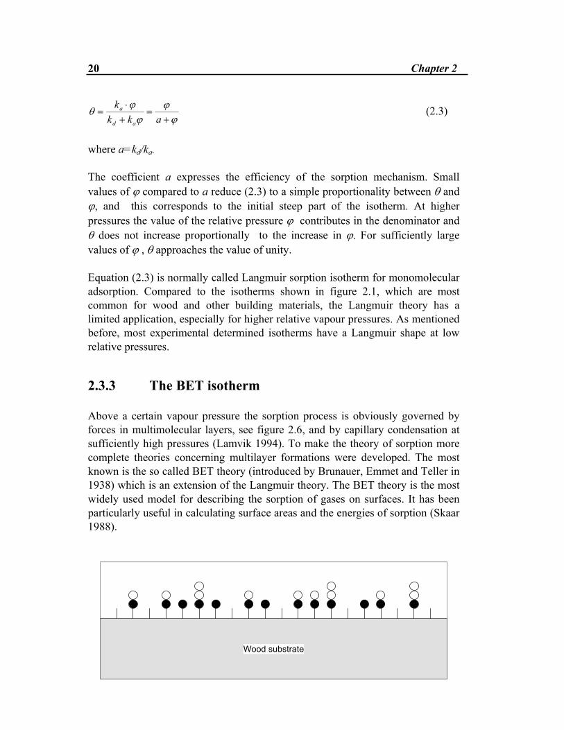
2.3.3 The BET isotherm Above a certain vapour pressure the sorption process is obviously governed by forces in multimolecular layers, see figure 2.6, and by capillary condensation at sufficiently high pressures (Lamvik 1994). To make the theory of sorption more complete theories concerning multilayer formations were developed. The most known is the so called BET theory (introduced by Brunauer, Emmet and Teller in 1938) which is an extension of the Langmuir theory. The BET theory is the most widely used model for describing the sorption of gases on surfaces. It has been particularly useful in calculating surface areas and the energies of sorption (Skaar 1988).
'������ �����

Sorption in Wood 21
Figure 2.6.: Schematic diagram showing primary sorption sites (vertical lines) in the cell wall, some of which are unoccupied and others occupied by primary water molecules (dark circles) and sometimes by secondary sorbed molecules (open circles). Adapted from Skaar (1988). The theory is based on the following assumptions (Saidani-Scott 1993): • In all layers except the first, the heat of adsorption is equal to the heat of
condensation. • In all layers except the first, the evaporation-condensation conditions are
identical. • When the pressure p=ps , the adsorbate condenses to a bulk liquid on the
surface of the solid, i.e. that the number of layers becomes infinite. The BET equation obtained is ( for derivation see e.g. Lamvik (1994)):
θ ϕϕ ϕ ϕ
=− − +
cc( )( )1 1
(2.4)
with
c aa
q qRT
L=−1 2
2 1
1νν
exp( ) (2.5)
where a1, a2 are constants, ν1, ν2 frequencies of molecule oscillations in a direction normal to the surface, R is the gas constant and T is the temperature. (q1-qL) is the differential heat of sorption, where q1 is the activation energy of the first layer and qL is the heat of condensation. In practice, the parameter c is nearly always taken equal to:
22 Chapter 2
cq q
RTL=
−exp( )1 (2.6)
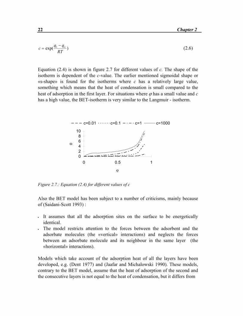
Equation (2.4) is shown in figure 2.7 for different values of c. The shape of the isotherm is dependent of the c-value. The earlier mentioned sigmoidal shape or «s-shape» is found for the isotherms where c has a relatively large value, something which means that the heat of condensation is small compared to the heat of adsorption in the first layer. For situations where ϕ has a small value and c has a high value, the BET-isotherm is very similar to the Langmuir - isotherm.
02468
10
0 0.5 1
ϕ
θ
c=0.01 c=0.1 c=1 c=1000
Figure 2.7.: Equation (2.4) for different values of c
Also the BET model has been subject to a number of criticisms, mainly because of (Saidani-Scott 1993) : • It assumes that all the adsorption sites on the surface to be energetically
identical. • The model restricts attention to the forces between the adsorbent and the
adsorbate molecules (the «vertical» interactions) and neglects the forces between an adsorbate molecule and its neighbour in the same layer (the «horizontal» interactions).
Models which take account of the adsorption heat of all the layers have been developed, e.g. (Dent 1977) and (Jaafar and Michalowski 1990). These models, contrary to the BET model, assume that the heat of adsorption of the second and the consecutive layers is not equal to the heat of condensation, but it differs from

Sorption in Wood 23
this heat by an additional heat, which is treated different in the different models. The models have the assumption that the extra heat is the same for all layers except the first. However, the mathematical formulation of the final equation is the same. Only the Dent model will be derived here.
2.3.4 The Dent model The Dent theory (Dent 1977), in common with the BET theory, postulates that water is sorbed in two forms. The first is in the form of «primary» water molecules strongly attached to specific or primary sorption sites with a high binding energy. The second form is as «secondary» water molecules attached to sites already occupied by primary water molecules or other secondary molecules. These are held by much weaker forces than those attached directly to primary sorption sites. The difference between the BET model and the Dent model is that the former model assumes that the thermodynamic properties of the secondary water are identical with those of ordinary liquid water, while the Dent model assumes that they are different. But both models assume that the properties of water in the various secondary layers, that means, the second, third, fourth, etc. layers, are identical. The model further assumes that the internal wood surface has a total area S available for sorption of water molecules. At a given moisture content a portion of this total area, S0, is free from water. The area S1 is covered with a monolayer, S2 with two layers, S3 with three layers and so on. See figure 2.8.
%� %� %� %� *��5
*��5
Figure 2.8.: Surface sorption model, showing the surfaces S0, S1, S2, etc. covered by 0, 1, 2, etc. layers of water molecules. Adapted from Dent (1977). When the internal wood surface is at equilibrium with water vapour in the surrounding atmosphere, the model presumes that there exists an equilibrium between the rate of condensation and evaporation of water at any layer. The rate of condensation on S0 is presumed to be equal to the rate of evaporation from S1. Also the condensation rate on S0 is taken to be proportional to the vapour pressure p, at constant temperature. The equilibrium between the rate of condensation on S0 and the evaporation on S1 can be written

24 Chapter 2
C S a p S0 1 0⋅ = ⋅ ⋅ (2.7) where a is an attachment rate constant per-unit-pressure which is assumed to be the same for all layers and C0 is the escape rate constant for the primary sites. By introducing another constant
b aC1
0
= (2.8)
equation (2.7) can be written S b p S1 1 0= ⋅ ⋅ (2.9) Similar equilibrium relationships are assumed to exist between other pairs of adjacent areas as follows: S b p SS b p SS b p S
S b p Si i i
2 2 1
3 3 2
4 4 3
1
= ⋅ ⋅= ⋅ ⋅= ⋅ ⋅
= ⋅ ⋅ −
............ (2.10)
It is further assumed that the proportionality coefficients bi are all equal to each other in all cases except for i = 1 (namely in the first layer). In other words b b b bi2 3 4= = =........ (2.11) The total internal surface area S is equal to S S S S S Si= + + + +0 1 2 3 ...... (2.12) The total possible volume V0 in the monolayer is given by V d S d S S S Si0 0 0 0 1 2= ⋅ = + + +( ........ ) (2.13)

Sorption in Wood 25
where d0 is the thickness of a single layer of water molecules. Then the total volume V in all layers is V d S S S iSi= + +0 1 2 32 3( ........ ) (2.14) With the assumption from equation (2.11) and the ratio S b p Si i i= ⋅ ⋅ −1 , i≠1 (2.15) equation (2.13) and (2.14) can be written as
[ ]V d S S b p b p b pi i i0 0 0 12 31= + + ⋅ + ⋅ + ⋅ +( ( ) ( ) ( ) .....) (2.16)
[ ]V d S b p b p b pi i i= ⋅ + ⋅ + ⋅ + ⋅ +0 1
2 31 2 3 4( ) ( ) ( ) .... (2.17) The binomial theorem states that
[ ]( ( )) ( ) ( ) ( ) .....1 11 2 3− ⋅ = + ⋅ + ⋅ + ⋅ +−b p b p b p b pi i i i (2.18)
[ ]( ( )) ( ) ( ) ( ) .....1 1 2 3 42 2 3− ⋅ = + ⋅ + ⋅ + ⋅ +−b p b p b p b pi i i i (2.19) Combining equations (2.16) - (2.19), the ratio V/V0 can be written
( ) ( )VV
Sb p
S Sb p
i i0
12 0
1
1 1=− ⋅
+ − ⋅
( ) ( ) (2.20)
Eliminating S1 by use of equation (2.9) and rearranging, equation (2.20) becomes
[ ]VV
b pb p b p b pi i0
1
11 1=
⋅− ⋅ ⋅ − ⋅ + ⋅( ) ( )
(2.21)
Equation (2.21) can be written in terms of wood moisture content u if it is assumed that the ratios u/u0=V/V0, where u0 is the moisture content corresponding to complete monolayer coverage of all available sorption sites. Thus,
26 Chapter 2
[ ]uu
b pb p b p b pi i0
1
11 1=
⋅− ⋅ ⋅ − ⋅ + ⋅( ) ( )
(2.22)
Equations (2.21) and (2.22) give the ratio of the total moisture content of the wood to that of the completely filled monolayer. It is generally more useful to re-express the pressure p in equation (2.22) as a relative pressure (relative humidity) ϕ=p/ps, where ps is the saturated vapour pressure, and so that ϕ varies only from 0 to 1. Thus a more useful form of equation (2.22) is:
[ ]uu
bb b bi i0
1
11 1=
⋅− ⋅ ⋅ − ⋅ + ⋅
ϕϕ ϕ ϕ( ) ( )
(2.23)
The special case where bi=1 gives
[ ]uu
bb0
1
11 1=
⋅− ⋅ − + ⋅
ϕϕ ϕ ϕ( ) ( )
(2.24)
which is the BET equation. The case where bi=0 gives uu
bb0
1
11=
⋅+ ⋅
ϕϕ
(2.25)
which is the Langmuir equation. The equations derived above include the total moisture content consisting of two components, primary and secondary water. An equation for the primary water can be derived using the following relationship for the volume V1 of primary water V d S S S Si1 0 1 2 3= + + +( ...... ) (2.26) By using the equations (2.9), (2.13), (2.16) and (2.18) and rearranging it can be shown that VV
uu
bb bi
1
0
1
0
1
11= =
⋅− ⋅ + ⋅
ϕϕ ϕ
(2.27)
Sorption in Wood 27
The secondary water can be obtained by subtracting equation (2.27) from (2.22) uu
u uu
b bb b b
i i
i i0
1
0
12
11 1=
−=
⋅ ⋅− ⋅ − ⋅ + ⋅
ϕϕ ϕ ϕ( )( )
(2.28)
Equations (2.27) and (2.28) give the primary and secondary moisture contents u1 and ui as functions of the three constants b1, bi and u0 , and of the relative vapour pressure ϕ . The constants b1 and bi are equilibrium constants relating the primary and secondary water to liquid water, u0 is the moisture content corresponding to complete monolayer coverage of all available sorption sites. The sum of the u1 and ui is equal to the total moisture content u. When the three constants are known, the sorption isotherm can be predicted. However, the sorption isotherm is usually measured experimentally, from which the three constants can be evaluated. To obtain a sigmoid sorption isotherm of the form
uA B C
=+ ⋅ − ⋅
ϕϕ ϕ 2 (2.29)
the three constants b1, bi and u0 have to be included in the new constants A, B and C. From equation (2.23) the new constants can be derived and shown to be
Au b
B b bu b
C b b bu b
i
i i
=⋅
=−⋅
=⋅ −⋅
1
20 1
1
0 1
12
0 1
(2.30)
If the measured sorption isotherm is plotted with ϕ/u along the vertical axis against ϕ along the horizontal axis, a parabola of the form ϕ ϕ ϕu
A B C= + ⋅ − ⋅ 2 (2.31)
can be fitted to the plotted points and the values of the empirical constants A, B and C can be calculated using linear regression techniques. As can be seen, this is
28 Chapter 2
the same mathematical expression as achieved by the Hailwood and Horrobin model.
2.4 Hysteresis
2.4.1 Theory The full sorption isotherms (absorption and desorption) at a given temperature define the limiting equilibrium values and thus may be viewed not as equilibrium loci, but as borders that outline the hysteresis area. Hence, the full cycle isotherms should be aptly referred to as boundary isotherms (Peralta 1995a). The hysteresis loop for wood has been shown to span over practically the full range of relative vapour pressures. The influence of hysteresis depends on the way the moisture equilibrium curves are made. The complete isotherms, as defined in (Skaar 1979), are those obtained from complete dryness and near saturation. Curves made over smaller humidity ranges, intermediate isotherms, tend to fall between the complete isotherms. Different mechanisms of sorption are dominating at different stages of the isotherms. Because of this different explanations of the hysteresis at the different relative humidities can be found. Three explanations, all based on the capillary theory of adsorption, have been given to explain hysteresis in rigid sorbents according to Cohan (1944), namely • The Incomplete Wetting Theory • The Bottle Neck Theory • The Open Pore Theory The theories mentioned above are all related to capillary condensation, but according to Ahlgren (1972) the process of capillary condensation is only decisive for hysteresis above 40 % relative humidity. Capillaries of the type considered by the Kelvin equation cannot occur at low relative humidities, since calculated capillary radii approaches the order of magnitude of molecular dimensions. Relative humidites below 40 % must have to do with variations in
Sorption in Wood 29
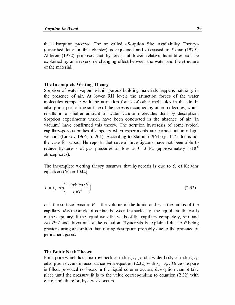
the adsorption process. The so called «Sorption Site Availability Theory» (described later in this chapter) is explained and discussed in Skaar (1979). Ahlgren (1972) proposes that hysteresis at lower relative humidities can be explained by an irreversible changing effect between the water and the structure of the material. The Incomplete Wetting Theory Sorption of water vapour within porous building materials happens naturally in the presence of air. At lower RH levels the attraction forces of the water molecules compete with the attraction forces of other molecules in the air. In adsorption, part of the surface of the pores is occupied by other molecules, which results in a smaller amount of water vapour molecules than by desorption. Sorption experiments which have been conducted in the absence of air (in vacuum) have confirmed this theory. The sorption hysteresis of some typical capillary-porous bodies disappears when experiments are carried out in a high vacuum (Luikov 1966, p. 201). According to Stamm (1964) (p. 147) this is not the case for wood. He reports that several investigators have not been able to reduce hysteresis at gas pressures as low as 0.13 Pa (approximately 1⋅10-6 atmospheres). The incomplete wetting theory assumes that hysteresis is due to θ, of Kelvins equation (Cohan 1944)
p p Vr RTS
c
=−
exp cos2σ θ (2.32)
σ is the surface tension, V is the volume of the liquid and rc is the radius of the capillary. θ is the angle of contact between the surface of the liquid and the walls of the capillary. If the liquid wets the walls of the capillary completely, θ=0 and cos θ=1 and drops out of the equation. Hysteresis is explained due to θ being greater during absorption than during desorption probably due to the presence of permanent gases. The Bottle Neck Theory For a pore which has a narrow neck of radius, rn , and a wider body of radius, rb, adsorption occurs in accordance with equation (2.32) with rc= rb . Once the pore is filled, provided no break in the liquid column occurs, desorption cannot take place until the pressure falls to the value corresponding to equation (2.32) with rc =rn and, therefor, hysteresis occurs.

30 Chapter 2
The Open Pore Theory In the case of a pore open at both ends, liquid cannot condense at the equilibrium vapour pressure given by equation (2.32) because a meniscus cannot form. The pressure, p, at which the meniscus forms, depends on the radius of curvature, r, of the cylindrical film on the wall of the capillary, that is (Cohan 1944)
p p VrRT
p Vr d RTS S
c
=−
=
−−
exp exp
( )σ σ
0
(2.33)
where rc is the radius of the pore and d0 the thickness of the adsorbed film which according to the capillary theory would be monomolecular; i.e. d0 would be the height of a sorbate molecule in a direction perpendicular to the surface. Once condensation has occurred a meniscus is present and the pressure, pd , at which evaporation occurs is given by equation (2.32). The Sorption Site Availability Theory The theory was originally given by Urquhart and Williams in 1958 (Stamm 1964). This theory (described in Skaar 1979) is based on the reduction in the availability of hydroxyl sorption sites on wood, which is absorbing moisture after having been dried. These hydroxyl groups are believed to be the primary, though not necessarily the only, sorption sites for the attachment of water molecules in the accessible region in the cell wall. According to this theory, the hydroxyl groups in green or water saturated wood, are attached to water molecules. When the wood dries some of the hydroxyl groups are freed from the attached water molecules and mutually bond with each other as they draw closer due to shrinkage. When water is regained or adsorbed, some of the hydroxyl groups are no longer easily available to bond with water molecules. This results in less adsorption of water at a given relative humidity compared with the initial desorption. As the relative humidity is increasing and additional water is taken up, the swelling pressure tends to break some of the hydroxyl-hydroxyl bonds. This is assumed to free some, but not all, of the originally water-bonded hydroxyl groups or sorption sites. These are then available to be rehydrated or to adsorb water molecules. During subsequent or secondary desorption the isotherm is higher than for absorption. However, it is generally lower than during initial desorption from green condition. This process repeats itself during subsequent cycling of the relative humidity, forming a more or less repetitive hysteresis loop, see e.g. figure 2.1.
Sorption in Wood 31
2.4.2 Absorption-Desorption ratios
The difference between the reproducible absorption and desorption isotherms is termed sorption hysteresis, often expressed in terms of the ratio A/D, where A is the absorption moisture-content value and D is the desorption value for a given value of the relative humidity. This is a general criterion for the extent of the sorption hysteresis on hygroscopic materials.
The complete absorption and desorption isotherms, which are obtained from complete dryness and near saturation, respectively, give the greatest A/D ratio. As an average for wood, the A/D ratio usually ranges between 0.75 and 0.85 (Schniewind 1989).
Several factors may enter into the variation in sorption hysteresis as measured by the A/D ratio. These factors include (Skaar 1979):
• Incomplete attainment of equilibrium • Immediate past history (e.g. number of absorption steps and possibly time at
each step) • Temperature • Physiochemical differences in the cell wall • Extractive content etc.
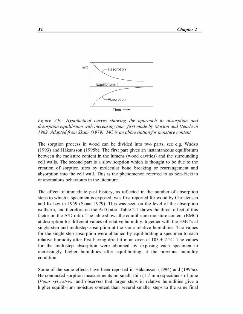
Incomplete attainment of equilibrium, either in absorption or description would tend to decrease the A/D ratio. Figure 2.9, shows the effect of time on the attainment of equilibrium from both desorption and absorption, assuming that the process of attaining equilibrium is an exponential function of time. It may require weeks or even months to attain equilibrium. This has e.g. been shown by Christensen (1965) and Wadsø (1993). This may be due to the fact that slow molecular rearrangements may be occurring in the wood as the structure accommodates itself to swelling forces (Skaar 1988).
32 Chapter 2
�- 6����&����
*,��� ����
� ���&����
7��� Figure 2.9.: Hypothetical curves showing the approach to absorption and desorption equilibrium with increasing time, first made by Morton and Hearle in 1962. Adapted from Skaar (1979). MC is an abbreviation for moisture content. The sorption process in wood can be divided into two parts, see e.g. Wadsø (1993) and Håkansson (1995b). The first part gives an instantaneous equilibrium between the moisture content in the lumens (wood cavities) and the surrounding cell walls. The second part is a slow sorption which is thought to be due to the creation of sorption sites by molecular bond breaking or rearrangement and absorption into the cell wall. This is the phenomenon referred to as non-Fickian or anomalous behaviours in the literature. The effect of immediate past history, as reflected in the number of absorption steps to which a specimen is exposed, was first reported for wood by Christensen and Kelsey in 1959 (Skaar 1979). This was seen on the level of the absorption isotherm, and therefore on the A/D ratio. Table 2.1 shows the direct effect of this factor on the A/D ratio. The table shows the equilibrium moisture content (EMC) at desorption for different values of relative humidity, together with the EMC’s at single-step and multistep absorption at the same relative humidities. The values for the single step absorption were obtained by equilibrating a specimen to each relative humidity after first having dried it in an oven at 103 ± 2 °C. The values for the multistep absorption were obtained by exposing each specimen to increasingly higher humidities after equilibrating at the previous humidity condition. Some of the same effects have been reported in Håkansson (1994) and (1995a). He conducted sorption measurements on small, thin (1.7 mm) specimens of pine (Pinus sylvestris), and observed that larger steps in relative humidities give a higher equilibrium moisture content than several smaller steps to the same final
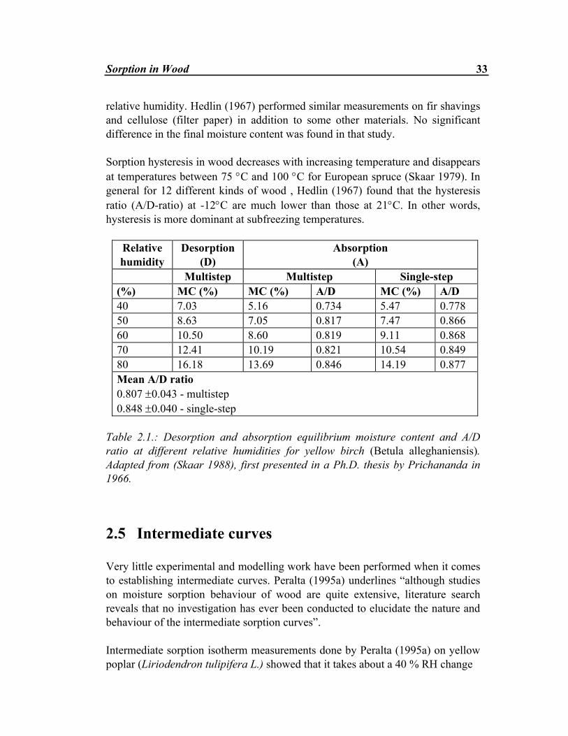
Sorption in Wood 33
relative humidity. Hedlin (1967) performed similar measurements on fir shavings and cellulose (filter paper) in addition to some other materials. No significant difference in the final moisture content was found in that study. Sorption hysteresis in wood decreases with increasing temperature and disappears at temperatures between 75 °C and 100 °C for European spruce (Skaar 1979). In general for 12 different kinds of wood , Hedlin (1967) found that the hysteresis ratio (A/D-ratio) at -12°C are much lower than those at 21°C. In other words, hysteresis is more dominant at subfreezing temperatures.
Relative humidity
Desorption (D)
Absorption (A)
Multistep Multistep Single-step (%) MC (%) MC (%) A/D MC (%) A/D 40 7.03 5.16 0.734 5.47 0.778 50 8.63 7.05 0.817 7.47 0.866 60 10.50 8.60 0.819 9.11 0.868 70 12.41 10.19 0.821 10.54 0.849 80 16.18 13.69 0.846 14.19 0.877 Mean A/D ratio 0.807 ±0.043 - multistep 0.848 ±0.040 - single-step
Table 2.1.: Desorption and absorption equilibrium moisture content and A/D ratio at different relative humidities for yellow birch (Betula alleghaniensis). Adapted from (Skaar 1988), first presented in a Ph.D. thesis by Prichananda in 1966.
2.5 Intermediate curves Very little experimental and modelling work have been performed when it comes to establishing intermediate curves. Peralta (1995a) underlines “although studies on moisture sorption behaviour of wood are quite extensive, literature search reveals that no investigation has ever been conducted to elucidate the nature and behaviour of the intermediate sorption curves”. Intermediate sorption isotherm measurements done by Peralta (1995a) on yellow poplar (Liriodendron tulipifera L.) showed that it takes about a 40 % RH change
34 Chapter 2
before the intermediate desorption isotherm join the boundary desorption isotherm. He further reports that as for textile fibres (cotton and wool), the length of the cross-over for wood is independent of the reversal point on the absorption isotherm. The intermediate desorption isotherms were obtained by preconditioning different sets of dried specimens to different initial moisture contents. The moisture contents corresponded to relative humidities of 92 %, 75 %, 53 %, and 32 % on the border absorption isotherm. After that the same sets of specimens were exposed to successively reduced relative humidity stages of about 10 % decrement down to 11% RH. For all cases, it took about a 40 % RH change before the intermediate desorption isotherm joined the boundary desorption isotherm. Of the intermediate isotherms generated, only the one reversed from absorption to desorption at 92 % RH showed the characteristic sigmoidal shape of the complete boundary isotherm. The intermediate isotherms whose reversal point corresponded to relative humidities of 75 %, 53 % and 32% were concave towards the x-axis. The significance of these results lies in the fact that if the immediate history of a piece of wood is not known, it is imperative to precondition the specimen in an atmosphere which is at least 40 % (RH) higher than the desired RH value. This is done in order to obtain a final moisture content that would fall on the boundary absorption isotherm (Peralta 1995a). In practice this means that one is not able to positively reach the border absorption isotherm above 60 % relative humidity. Ahlgren (1972) has also measured two intermediate isotherms for spruce (Picea abies). One curve originates from 44 % RH on the desorption isotherm and reaches the absorption isotherm at 95 % RH, about a 50 % RH change before the border absorption isotherm was reached. However, as can also be seen in figure 2.10, the absorption isotherm is almost reached around 70 % RH, only small differences between the absorption isotherm and the intermediate curve exist. The intermediate curve (consisting of 4 measured values) is convex towards the x-axis. The other curve is from the 98 % RH level on the absorption isotherm, but this has not been shown in any figures because it has already joined the border desorption isotherm at 90 % RH. The starting point here is 8 % relative humidity above the corresponding starting point in Peralta’s experiment, and Ahlgren indeed came to a different conclusion. Although Ahlgren has made two intermediate curves only, it shows that no general conclusion on how these intermediate curves are can be drawn.
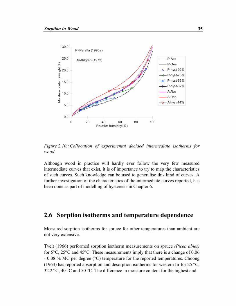
Sorption in Wood 35
0.0
5.0
10.0
15.0
20.0
25.0
30.0
0 20 40 60 80 100Relative humidity (%)
Moi
stur
e co
nten
t (w
eigh
t %)
P-Abs
P-Des
P-hyst-92%
P-hyst-75%
P-hyst-53%
P-hyst-32%
A-Abs
A-Des
A-hyst-44%
P=Peralta (1995a)
A=Ahlgren (1972)
Figure 2.10.: Collocation of experimental decided intermediate isotherms for wood. Although wood in practice will hardly ever follow the very few measured intermediate curves that exist, it is of importance to try to map the characteristics of such curves. Such knowledge can be used to generalise this kind of curves. A further investigation of the characteristics of the intermediate curves reported, has been done as part of modelling of hysteresis in Chapter 6.
2.6 Sorption isotherms and temperature dependence Measured sorption isotherms for spruce for other temperatures than ambient are not very extensive. Tveit (1966) performed sorption isotherm measurements on spruce (Picea abies) for 5°C, 25°C and 45°C. These measurements imply that there is a change of 0.06 - 0.08 % MC per degree (°C) temperature for the reported temperatures. Choong (1963) has reported absorption and desorption isotherms for western fir for 25 °C, 32.2 °C, 40 °C and 50 °C. The difference in moisture content for the highest and
36 Chapter 2
lowest temperature at the same relative humidity is between 2 and 3 weight %. The biggest difference is found for the higher relative humidities in absorption. This implies that there is an approximate change of 0.1 weight % per degree (°C) temperature change for temperatures from 25 °C to 50 °C. Desorption isotherms for wood for at 20°C, 40°C, 60°C and 80°C are presented in the Sorption Isotherm Catalogue edited by Hansen (1986). An average change in moisture content per degree (°C ) change in temperature is found to vary between 0.03 and 0.05 weight %. In Keey (1978) a general empirical formula is given for how to calculate the variations in equilibrium moisture content according to temperature for a given relative humidity ∂∂
uT
A uRH
= − ⋅ (2.34)
The coefficient A lies between 0.005 and 0.01 °C-1 for relative humidities between 10 % and 90 % for materials such as natural and synthetic fibres, wood and potatoes (Keey 1978). An approximate calculation for spruce at 50 % RH gives a change in moisture content per degree °C equal to 0.05 weight % (A is assumed equal to 0.0075) if the temperature decreases from 20 °C to 0°C. The shape of the sorption isotherms for the different temperatures given by Choong (1963) are very much the same, this is also the case for the desorption isotherms reported in Hansen (1986). Hedlin (1967) has reported sorption isotherms for twelve different kinds of wood at subfreezing temperatures. Spruce (type not given) was one of the kinds. A summary for spruce is shown in figure 2.11 for the 3 different temperatures -16°C, -12°C and 21°C. Note that at a relative humidity of about 99 % relative to ice, the moisture content reached at -12°C, were substantially lower than those reached at about the same relative humidity at 21°C. This trend was the same for all species. A practical consequence of this is that wood used as exterior cladding will tend to have a moisture content below that of fibre saturation during the winter season if the temperature is below zero.

Sorption in Wood 37
0
5
10
15
20
25
30
0 20 40 60 80 100
Relative humidity (%)
Moi
stur
e co
nten
t (w
eigh
t %)
Absorp -12 Desorp -12 Absorp-16
Desorp -16 Absorp 21 Desorp 21
EMC (=23 %) at -12C and 99 % RHrelative to ice,in absorption
Figure 2.11: Sorption isotherm data for spruce at -12°C, -16°C and 21°C reported by Hedlin (1967).
2.6.1 Influence of drying temperature on sorption isotherms In practice it is not possible to distinguish the amount of water physically bound and chemically bound. Instead we speak about water which can evaporate and water which cannot. The limit between these two is determined by a standardised way of drying test specimens (Ahlgren 1972). The most common way of doing this is by oven drying at 105 °C. In CEN (1995) another drying procedure is proposed. For organic materials e.g. wood, where changes in structure due to thermal influences may occur, the drying temperature is set to 70 ± 2 °C. In general, moisture-sorption isotherms are measured at room temperature. An increase in the temperature affects the hygroscopicity of wood in two ways. The first or immediate effect is to reduce the equilibrium moisture content at any constant relative humidity. This is a more or less reversible effect. The second or long-term effect of exposing wood to high temperatures, particularly above 100 °C, is a permanent reduction in hygroscopicity when the wood is brought back to room temperature.

38 Chapter 2
Kollmann (1961) presents sorption isotherms of spruce after pre-treatment with different temperatures for 24 hours. The temperatures varied between 70 °C and 200 °C. The difference in equilibrium moisture content for wood dried between 70°C and 100°C is very little, but for differences in drying temperature between 100°C and 200°C, the difference is relatively large. Kurtoglu (1983) reports about a comparison of sorption isotherms for green, heat treated (in 100 °C for 2 weeks and 4 weeks) and 100 years old spruce (Picea excelsa). Above 40 % relative humidity the old wood had the lowest EMC while the green wood had the highest EMC. However along the whole range of the RH scale the difference was at a maximum 2 weight %, which is not very much as the isotherms are both desorption (from green) and absorption (the heat treated ).
2.7 Sorption isotherm measurements on spruce (Picea abies) performed in the Nordic countries Some sorption measurements on spruce (Picea abies) have been performed in the Nordic countries throughout the last 30 years. An investigation of these has been made. The reported measurements have been compared with each other and they have been compared with sorption measurements performed by the author in this project. Tveit (1966) did measurements with 14 different combinations of temperature and relative humidity within the range of 5 - 45 °C and 10 - 97 % RH respectively. Two parallel circular test specimens, 80 mm in diameter and 13 mm in thickness have been exposed to either of the 14 combinations. The isotherms are a combination of an absorption and a desorption isotherm. At first the test specimens were equilibrated at 75 % relative humidity from a wet condition. Successive tests were then carried out at approximately 55%, 35%, 12% (which means on the desorption isotherm) and at last 95 % RH (which means on an absorption isotherm). Due to difficulties in predicting the accurate RH in the chamber for each step, it was impossible strictly to follow a desorption isotherm. The valid data (read from the original graph) for 25 °C has been fitted to the Hailwood and Horrobin model and presented in figure 2.12 and 2.13.
Sorption in Wood 39
Tveit (1966) has actually reported a desorption isotherm from 75 % RH down to 12 % RH, and one single value for 95 % RH only, on an absorption isotherm. Ahlgren (1972) comments as the hysteresis are of less importance at lower RH, the equilibrium curves from Tveit (1966) are according to the absorption isotherm. But regarding the results from the sorption isotherm measurements of e.g., Liu Tong (1989) and Absetz (1993), there is a significant effect of hysteresis also in the lower RH region, and Tveit’s isotherms must be regarded as a desorption isotherm from 75 % RH, or it can be regarded as a sorption isotherm if it is of less importance to differ between absorption and desorption. Ahlgren (1972) performed sorption measurements for a selection of building materials, including spruce. The measurements have been performed in a so called «two-pressure-apparatus» (for further description see Ahlgren (1972)). Two or three separate specimens of unknown size have been used for the experiments. To obtain the first desorption isotherm the specimens have been saturated before the measurements started. For most materials vacuum has been used to saturate the material, presumably this is the case for spruce too. The absorption measurements have started with drying the specimens in an evacuated exicator with a drying agent (silica gel or dehydrit). Most of the specimens were dried in a drying chamber at 105 °C to decide the dry weight (unsure if this was the case for spruce). Others were dried at a lower temperature or in an evacuated exicator with a drying agent. The whole experiment (absorption and desorption isotherms) took about one year. The measurements are presented in Ahlgren (1972) and in the Sorption Isotherm Catalogue edited by Hansen (1986). Morén and Sehlstedt (1984) conducted desorption measurements of both spruce and pine of Nordic origin. They measured the first or the initial desorption isotherm (from green condition) in addition to a desorption isotherm from resaturation. Altogether 51 specimens were included in the initial experiment. The standard deviation for the moisture content at the different levels varied between ± 0.1 weight % and ± 0.3 weight %. No significant difference was found between the moisture contents for the two different desorption isotherms, from green and resaturated conditions respectively. No correlation between moisture content in spruce and density was found. Liu Tong (1989) has done sorption measurements on spruce and pine grown in Sweden. Only one specimen of each kind (e.g. for sapwood in absorption) has been tested. He has come to the conclusion that there is hardly any difference in

40 Chapter 2
absorption or desorption neither for spruce nor pine, both sapwood and heartwood. Similar sorption measurements have been reported by Absetz (1993). He found a significant difference in EMC for sapwood and heartwood of pine, but none for spruce. He also found that the hysteresis was somewhat bigger for spruce than for pine. Støre (1996) has, in association with her work on moisture transport in painted substrates, reported sorption isotherms for spruce. According to Støre (1997, personal communication) the reported values might not be final equilibrium values, although parallel specimens (approximately 50 x 50 x 5 mm3 ) have been equilibrated simultaneously at different RH for 30 days. Desiccant drying (Calcium-chloride) has been used. From figure 2.12 it can be seen that the reported results are on the extreme border, something which might confirm that the final equilibrium values have not been reached. Because of reported uncertainties in the data , they have not been fitted to the Hailwood and Horrobin model. Sorption isotherm measurements on spruce have also been done in this work. Absorption isotherm data for seven different relative humidities are reported and desorption isotherm data for four different relative humidities. The desorption isotherm is only valid from below 75 % relative humidity as mould growth made us omit higher relative humidities. The highest value on the absorption isotherm is not necessarily the final moisture equilibrium either, as we had to stop the experiment on the 97 % level after approximately 700 hours because of mould growth. The obtained moisture equilibrium values are presented in figure 2.12 and 2.13. From figure 2.12 it can be seen that there is very little difference between the desorption data and the absorption data reported in this project. For the lowest relative humidity level the absorption value is even higher than the desorption value. The assumed lowest relative humidity (obtained by the aid of calcium-chloride) is outside the validity range of the RH sensor (Vaisala HMD 30 Y) and might in that sense be an incorrect value. According to Burch (1997, personal communication), it is very important to treat calcium-chloride in a correct way in order to obtain a relative humidity below 1.5 % RH. In this work a value of 5 % RH has been measured. Reasons why the desorption data has reached such low values might be explained by the following: During the performance of the desorption isotherm data, the temperature conditions have reached above 30°C occasionally. Another explanation might have to do with the fact that the specimens have been affected by mould growth. Only four values in

Sorption in Wood 41
desorption, all below 75 % RH are reported, because of this only the absorption isotherm data are fitted to the Hailwood and Horrobin model. The results are presented in full in Bergheim et al. (1998).
Reference
Sorpa, Abs.,
or Des (number of measuring
points)
A
B
C
SR/n
Tveit (1966)b Sorp (5) 1,047315 0,130558 0,001079 0,285 Tveit (1966)c Sorp (5) 1.273390 0,121262 0,001009 0,181
Ahlgren (1972) Abs (11) 1,388877 0,138648 0,001194 1.080 Ahlgren (1972) Des (14) 1.794265 0,083227 0,000692 0,051 Morèn (1984) Des (5) 4,489897 0,010285 0,000190 0,209
LiuTong(1989) Abs (7) 2,235632 0,190302 0,001800 0,279d LiuTong(1989) Des (7) 1,215461 0,121667 0,000930 0,163d Absetz (1993)e Abs (7) 3,380826 0,116223 0,001060 0,046d Absetz (1993)e Des (7) 0,697183 0,162572 0,001380 0,587d
This work Abs(7) 0,584371 0,156113 0,001151 0,780 a; a combination of an absorption and a desorption isotherm b; the density of the specimens is 410 kg⋅m-3 c; the density of the specimens is 450 kg⋅m-3 d; a curve fit to the Hailwood and Horrobin model is shown in the source reference too. The parameters and the SR/n differ from the values obtained in this work. e; measuring points are read from a graphical presentation. Table 2.2: Curve fitting parameters found for data given by different references to express sorption isotherms for spruce by the Hailwood and Horrobin model. The sum of squares of residuals (SR) divided by the number of measuring points (n) is also presented to show how well the different sets of data fit the model. The moisture equilibrium values reported by the different researchers have been fitted to the Hailwood and Horrobin model and can be seen in figure 2.12 and 2.13. Figure 2.12 presents a collocation of the measured moisture equilibrium values obtained , while figure 2.13 shows the Hailwood and Horrobin adjustment obtained by the measured values. The obtained curve fit parameters for the different measured values are shown in table 2.2. The table also contains a value for the sum of squares of residuals divided by the number of measuring points for
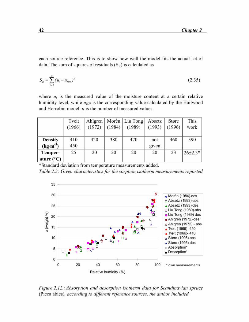
42 Chapter 2
each source reference. This is to show how well the model fits the actual set of data. The sum of squares of residuals (SR) is calculated as
S u uR i HHi
n
= −=∑( )2
1
(2.35)
where ui is the measured value of the moisture content at a certain relative humidity level, while uHH is the corresponding value calculated by the Hailwood and Horrobin model. n is the number of measured values.
Tveit (1966)
Ahlgren(1972)
Morèn(1984)
Liu Tong(1989)
Absetz (1993)
Støre (1996)
This work
Density (kg⋅m-3)
410 450
420 380 470 not given
460 390
Temper-ature (°C)
25 20 20 20 20 23 26±2.3*
*Standard deviation from temperature measurements added. Table 2.3: Given characteristics for the sorption isotherm measurements reported
0
5
10
15
20
25
30
35
0 20 40 60 80 100
Relative humidity (%)
u (w
eigh
t %)
Morén (1984)-desAbsetz (1993)-absAbsetz (1993)-desLiu Tong (1989)-absLiu Tong (1989)-desAhlgren (1972)-desAhlgren (1972) - absTveit (1966)- 450Tveit (1966)- 410Støre (1996)-absStøre (1996)-desAbsorption*Desorption*
* own measurements
Figure 2.12.: Absorption and desorption isotherm data for Scandinavian spruce (Picea abies), according to different reference sources, the author included.

Sorption in Wood 43
Figure 2.12 shows that there is a rather great variation in moisture equilibrium values among the different sources. For relative humidities above 70 % the gap between the different sources is at its most. The difference in moisture content between the lowest absorption isotherm and the highest desorption isotherm is more than 8 weight %.
0
5
10
15
20
25
30
35
0 20 40 60 80 100Relative humidity (%)
u (w
eigh
t %)
Tveit (1966)Tveit (1966)Ahlgren (1972)-absAhlgren (1972)-desLiuTong (1989)-absLiuTong (1989)-desAbsetz (1993)-absAbsetz (1993)-desMorén (1984)-desTime* -abs
* from own measurements
Figure 2.13.: Absorption and desorption isotherm data for Scandinavian spruce reported by different researchers (Picea abies) fitted to the Hailwood and Horrobin model.
2.8 Sorption in wood related to building physics and - engineering practice Sorption isotherm data is required for many purposes in the building industry. In timber seasoning it is necessary to know to which conditions the wooden boards
44 Chapter 2
shall be dried. For wood to be used indoor it is important that the material is in reasonable equilibrium with indoor conditions before use. To prevent wooden boards used as flooring material from shrinkage and swelling, to maintain a neat floor without defects, it is important that the moisture condition of the boards is in equilibrium with the indoor air. The hazard of rot is often a performance criterion in buildings. It is often assumed that if the moisture content in wood is kept below 20 weight % rot will not occur. According to figure 2.12 a moisture content of 20 weight %, can be achieved with the RH from approximately 75 - 80 % RH. A thumb rule is that you shall not expose wood to relative humidities above 80 % for a longer period of time as this is seen as a limit for mould growth. According to figure 2.12 the moisture content of wood can be in the range of 14 to 20 weight %, for a relative humidity of 80 %. For some building materials there is little difference between the absorption and the desorption isotherm, and only one isotherm for characterising the equilibrium moisture condition is sufficient. This is not the case for wood. The necessity of considering hysteresis in practice is not well proved. In many situations an average isotherm between absorption and desorption may well be used. Considering the reported data in chapter 2.7 there is a rather great variation in equilibrium moisture content for spruce both in absorption and desorption even at the same relative humidity. Some of these differences may be due to inaccuracies in the experimental procedures, but they may also be due to structural variations. Sorption isotherm measurements are very time consuming indeed, and because of this quite sensitive to temperature and humidity variations due to «failures» in the sorption apparatuses. One of the main problems regarding sorption in wood in building constructions and building envelopes is related to the immediate past history of wood. One rarely knows if the moisture conditions correspond to an absorption, a desorption or a hysteresis situation. The internal differences between the reported absorption isotherm values and the desorption isotherm values on one hand, and the reported hysteresis effect on the other hand are of a similar order of magnitude. The nature of hysteresis is not well known and hardly any calculation tools include hysteresis. For practical applications this fact leads to a choice: which level for the isotherms to choose, thereafter if hysteresis is to be considered. It is shown later in this report that the levels of the absorption and the desorption isotherm are of major importance when modelling relatively rapid cyclic moisture sorption in wood. It is also shown that best fit between measurements and calculations is obtained when taking hysteresis into account in the calculation model. Håkansson (1995b) has also shown by his model that best conformity between relatively slow cyclic sorption measurements and calculations on wooden specimens is achieved when considering hysteresis. The relatively large differences in level of

Sorption in Wood 45
the different absorption and desorption isotherms reported in chapter 2.7 should also confirm that the hysteresis effect for wood has to be considered when modelling moisture conditions in wooden building structures. To sum up; the equilibrium moisture content may vary significantly from one piece of wood to another at the same relative humidity. Absorption and desorption isotherms define borders that outline the hysteresis area. Quite a few models have been proposed throughout the years in order to explain and quantify the measured sorption isotherms. Most models still underpredict experimental obtained moisture contents for higher relative humidities. Rather significant differences in measured equilibrium moisture contents have been reported in the literature. This implies that different sorption isotherm levels, preferably including hysteresis, or a probabilistic approach should be considered when solving moisture sorption problems for wood.
Chapter 3
Moisture Transport in Wood - Theory and Experiences Moisture movement in wood can be divided into two main parts; the movement of liquid water above the fibre saturation point and the movement of bound water and water vapour below the fibre saturation point (hygroscopic moisture). This thesis is concerned with the latter part only. In this chapter is presented a theoretical background for hygroscopic moisture transport in wood. Different approaches, reported in the literature, for describing moisture transport processes are presented.
3.1 Moisture transport mechanisms The most common way of describing the quantitative aspects of moisture movements in wood is by assuming that the rate of moisture exchange is governed by diffusion processes (molecular diffusion). The diffusion coefficient in the transport equation is used to describe the flow rate of migrating moisture.
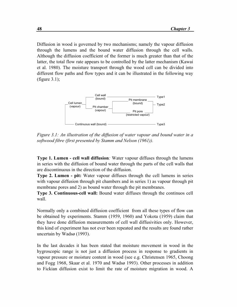
48 Chapter 3
Diffusion in wood is governed by two mechanisms; namely the vapour diffusion through the lumens and the bound water diffusion through the cell walls. Although the diffusion coefficient of the former is much greater than that of the latter, the total flow rate appears to be controlled by the latter mechanism (Kawai et al. 1980). The moisture transport through the wood cell can be divided into different flow paths and flow types and it can be illustrated in the following way (figure 3.1);
�������������
����������������
��������������
����������������
�����������������������
�����
�����
�����
����������������
Figure 3.1: An illustration of the diffusion of water vapour and bound water in a softwood fibre (first presented by Stamm and Nelson (1961)). Type 1. Lumen - cell wall diffusion: Water vapour diffuses through the lumens in series with the diffusion of bound water through the parts of the cell walls that are discontinuous in the direction of the diffusion. Type 2. Lumen - pit: Water vapour diffuses through the cell lumens in series with vapour diffusion through pit chambers and in series 1) as vapour through pit membrane pores and 2) as bound water through the pit membranes. Type 3. Continuous-cell wall: Bound water diffuses through the continuos cell wall. Normally only a combined diffusion coefficient from all these types of flow can be obtained by experiments. Stamm (1959, 1960) and Yokota (1959) claim that they have done diffusion measurements of cell wall diffusivities only. However, this kind of experiment has not ever been repeated and the results are found rather uncertain by Wadsø (1993). In the last decades it has been stated that moisture movement in wood in the hygroscopic range is not just a diffusion process in response to gradients in vapour pressure or moisture content in wood (see e.g. Christensen 1965, Choong and Fogg 1968, Skaar et al. 1970 and Wadsø 1993). Other processes in addition to Fickian diffusion exist to limit the rate of moisture migration in wood. A

Moisture Transport in Wood - Theory and Experiences 49
second process, apparently related to the rate of molecular rearrangement to permit the formation of new sorption sites, or to increase the size of microvoids for holding dissolved water (results in swelling), is superimposed on the classical Fickian behaviour (Skaar et al. 1970). The Fickian mechanism appears to be more dominant at low relative humidities, see e.g. Comstock (1963), Skaar et al. (1970) and Wadsø (1993), while the rate at which bonds can be broken is more important at high relative humidities when small moisture increments are involved (Skaar et al. 1970). The slow process is corresponding to the phenomenon often called non-Fickian (Wadsø 1993) or anomalous (Christensen 1965, Cunningham 1994) behaviours in wood. The two processes are of different time scales. The Fickian diffusion is instantaneous, while the process related to rearrangement of sorption sites or increase of the size of microvoids is a much more slow process.
3.1.1 Fick’s first law In spite of the fact that it has been known for the last decades that moisture transport in wood in the hygroscopic region is not governed by diffusion alone, the traditional diffusion equations, Fick’s first and second law, are still most often used to describe moisture transport in wood. It is also used for evaluation of diffusion coefficients from laboratory experiments. For the one-dimensional steady-state situation the vapour flow is usually calculated by Fick’s first law of diffusion;
F Dx
= − α∂α∂
(3.1)
Dα , is the diffusion coefficient with α as the driving potential. ∂α/∂x is the space gradient of the driving potential in one direction. The minus sign indicates that the transport is in the direction of a negative gradient, i.e. from high to low concentration. The diffusion coefficient can be described in many ways. The size and the unit of this coefficient depend upon the driving potential of the transport. The transport coefficient, Dα, in equation (3.1), is called either the diffusion coefficient, just the transport coefficient, the water vapour permeability or the diffusivity. These ways of expressing the transport coefficient have no meaning if the driving potential used is not stated. There are uncertainty and misunderstanding about these terms.
50 Chapter 3
3.1.2 Driving potentials Models based on a mechanistic approach, in which a macroscopic description of the transfer phenomena has been derived from Fick’s law, may have different driving potentials. The most widely used driving potential for diffusion in wood within wood science is moisture concentration in wood (symbol C, also expressed as moisture content by volume, kg⋅m-3) (Comstock 1963, Choong 1963, Biggerstaff 1965, Choong and Fogg 1968, Kawai 1978, Koponen 1986, Droin et al. 1988, Droin-Josserand et al. 1988, Wadsø 1993). To use the moisture content (symbol u, also expressed as moisture content by weight, kg⋅kg-1) is essentially the same as to use the moisture concentration. The diffusion coefficients with moisture concentration and moisture content as driving potential are written DC (m2⋅s-1) and Du (kg⋅m-1⋅s-1) respectively. Other potentials used to some extent in wood science is vapour pressure, water activity (i.e., relative humidity), chemical potential (or water potential), osmotic pressure and «spreading» pressure (Siau 1984, Skaar 1988). Skaar and Babiak (1982) proposed a model for isothermal transport of bound water through the cell wall of wood based on a gradient of «spreading» pressure. This pressure is a surface phenomenon, derivable from the surface sorption theory of Dent (1977) (see Chapter 2). The space gradient of this potential is expressed in terms of the relative humidity and constants related to the Dent isotherm. Kawai et al. (1980) have done a quantitative analysis of isothermal moisture movement in wood using chemical potential as the driving force. Their conclusion, in regards of their experimental work, is that the chemical potential is the essential driving force for moisture movement in wood. The chemical potential (for definition see section 3.3.2) has been more widely applied to non-isothermal conditions, and is further described in section 3.3. Cunningham (1994) has done a theoretical complement to the experimental investigations of Wadsø (1993). He has proposed a model, where moisture transfer in wood is regarded as a two-stage process: ordinary Fickian diffusion, and a non-Fickian process of slow sorption of moisture in the cell wall. A one-dimensional moisture conservation equation for the wood lumens is set up. ∂∂
∂∂
∂∂
ct x
Dl
lcx
h kw lcc= + −( ) ( ) (3.2)
Moisture Transport in Wood - Theory and Experiences 51
and for the cell wall ∂∂wt
h lc kw= −( ) (3.3)
The total moisture concentration, C, is C= c + w (3.4) here C is the moisture concentration in wood (kg⋅m-3), c is the moisture concentration in the lumens (kg⋅m-3) and w is the moisture concentration in the wood cell walls (kg⋅m-3). Dc is the diffusion coefficient with lumen moisture concentration as driving potential. l, k and h are coefficients connected with the moisture concentration in the lumens and the cell walls respectively. By the means of simplifications he has shown that an analytical solution exists to the model equations above. The model describes isothermal conditions only. Because of this the coefficients l, k, h and Dc is only dependent of moisture concentration. In the reported solutions of the equations above, the coefficients are made constant. Håkansson (1995b) has proposed a model for isothermal transient moisture transport in wood in which the slow sorption effect is divided into two parts. The first part is called the instantaneous sorption and the other part the time-dependent sorption.. To model the time-dependent sorption, n internal levels (in the cell wall) are added to an outer layer in direct contact with the lumen. In order to consider non-Fickian effects, different types of moisture capacity and moisture transport coefficients are included in the internal levels. For a detailed description the reader is referred to Håkansson (1995b). A so called Kirchhoff potential, is introduced by Arfvidsson (1994). In association with drying of wood, a two-dimensional model (cylinder coordinates) for isothermal transient moisture transport in wood has been set up using this potential. A detailed explanation of the model can be found in Arfvidsson (1994). A building physics approach Within building technology and building physics, wood is most often only a part of a construction consisting of many layers of different materials with different properties. Moisture transport calculations in that respect include wood as well as

52 Chapter 3
other materials. The main interest is usually the influence of the overall moisture performance of the construction on critical layers; wooden studs for instance. It is therefore most useful to use a driving potential which is consistent for many materials, and which can be measured without interfering with the construction. The water vapour pressure (Pa) is such a potential and so is the water vapour content of the air (kg⋅m-3). An advantage by using the water vapour pressure or the water vapour content of the air as the driving potential, is that it represents continuity across layers of different materials, a wall for example. The diffusion coefficient with water vapour pressure as the potential, Dp (kg⋅m-1⋅s-1⋅Pa-1), can easily be transferred into a diffusion coefficient, Dv (m2⋅s-1), with water vapour content of the air as the potential by the relation D T Dv p= ⋅ ⋅461 4, (3.5) where T is the absolute temperature (Kelvin). Note that the diffusion coefficient with water vapour content of the air (kg⋅m-3) as potential and the diffusion coefficient with the moisture concentration of wood (kg⋅m-3) as a potential have the same unit, m2s-1.
3.2 Isothermal diffusion equations The notions steady-state and non-steady-state moisture flux are used to express whether the moisture flux is varying with time or not. Most situations are non steady-state, but for some cases in building physics it is accurate enough to regard it as steady-state situations. An example of a typical non-steady-state situation is drying of building moisture. An outer wall with no built-in-moisture can sometimes be regarded as having a steady-state moisture flow. For the isothermal one dimensional steady-state situation the equation is according to equation (3.1)
F D pxp= −∂∂
(3.6a)
or

Moisture Transport in Wood - Theory and Experiences 53
F D CxC= −
∂∂
(3.6b)
Here p is the water vapour pressure in the air (Pa), which gives a diffusion coefficient with vapour pressure as potential, Dp with unit (kg⋅m-1⋅s-1⋅Pa-1). C is the moisture concentration in wood (kg⋅m-3), which gives a diffusion coefficient with moisture concentration as potential, DC (m2 ⋅s-1).
3.2.1 Relations between coefficients If the moisture situation in wood is within the hygroscopic region it is so that the moisture concentration in wood is related to the relative humidity of the air, ϕ. Then we have; C C= ( )ϕ (3.7) At the same time we know that p ps= ⋅ϕ (3.8) where ps is the saturated vapour pressure at a certain temperature. (3.6a) can then be rearranged so that we have
F D pC
Cxp= − ⋅ ⋅
∂∂
∂∂
(3.9)
We can now introduce the diffusion coefficient with moisture concentration in wood as a potential;
D D pC
D p CC p p s= ⋅ = ⋅ ⋅∂∂ ∂
∂ϕ
1 (3.10)
The term ∂
∂ϕC is the slope of the sorption isotherm. In that sense the
interrelation between the two diffusion coefficients , Dp and DC , is in terms of the sorption isotherm, and the moisture flux can be expressed as in (3.6b). The
54 Chapter 3
relation between the moisture concentration in wood by volume, C, and the moisture content in wood by weight, u, is C u= ⋅ ρ 0 (3.11) if the hygral expansion is neglected (Liu Tong 1989). ρ0 is the dry density of wood. Differentiating the equation we get dC du= ⋅ρ 0 (3.12) This gives the relation
F D uxC= − ⋅ ⋅ρ ∂∂0 (3.13)
which can be expressed as
F D uxu= − ⋅∂∂
(3.14)
Corresponding relations can be found in Skaar (1988) between the above mentioned coefficients and the diffusion coefficient with either chemical potential, osmotic pressure or «spreading pressure». The coefficients for the transport of water vapour through wood may be measured by applying gradients of moisture content or partial vapour pressure.
3.2.2 Isothermal non steady-state moisture transport Differentiating the equation (3.6b) with respect to x, we get ∂∂
∂∂
∂∂
Fx x
D CxC= − ⋅
(3.15)
According to the law of mass conservation ∂∂
∂∂
Fx
Ct
= − (3.16)
Moisture Transport in Wood - Theory and Experiences 55
This gives the equation ∂∂
∂∂
∂∂
Ct x
D CxC= ⋅
(3.17)
which is often called Fick’s second law of diffusion. If the diffusion coefficient, DC, is a constant the equation reduces to ∂∂
∂
∂
Ct
D C
xC= ⋅
2
2 (3.18)
The corresponding form of the equation with vapour pressure as potential: ∂∂
∂∂
Ct
D pxp= ⋅2
2 (3.19)
3.3 Non-isothermal moisture movement
Over the years, many theoretical solutions to the problem of non-isothermal moisture movement in wood have been proposed in the society of wood science. They are most often either mechanistic in nature or they are based on principles of thermodynamics. Steady-state models can be found in e.g., Siau (1980), Skaar and Siau (1981), Siau (1983a) and Stanish (1986), while non-steady state models are proposed by Siau (1983b), Avramidis et al. (1992) and Avramidis et al. (1994). Verification of the models can only be done through good experimental measurements. However, not many reported sets of experimental data on non-isothermal moisture diffusion in wood are available. Voigt et al. (1940) and Choong (1963) have reported this kind of data, and more recent research results have been presented by Siau and co-workers (Siau and Babiak 1983, Siau and Jin 1985, Siau et al. 1986, Avramidis et al. 1987, Avramidis and Siau 1987). The most recent contributions are given by Peralta and Skaar (1993) and Avramidis et al. (1992, 1994). The above mentioned experimental results are all for the steady-state situation, only Avramidis et al. (1992,1994) have reported experimental results for non-isothermal transient conditions.
56 Chapter 3
Fick’s law has been used to quantify the movement of moisture in wood for non-isothermal conditions also. Bramhall (1976, 1979) tried to identify the proper driving force for moisture movement in wood. He attempted to explain the experimental results on non-isothermal diffusion obtained by Voigt et al. (1940) and Choong (1963) by using the steady-state form of Fick’s law with a vapour pressure gradient as the driving force instead of the more commonly used force in wood science, moisture concentration in wood. This approach resulted in a considerable controversy, which precipitated a lively exchange of ideas in the wood science literature and led to a renewed interest in the subject of non-isothermal moisture movement in wood (Stanish 1986, Peralta and Skaar 1993).
3.3.1 A building physics approach A difference in temperature will also be a driving force for diffusion. In building physics a mechanistic approach has been used to express this part of the moisture transport (Kumaran 1991, Trechsel 1994):
F D TxT T= − ⋅
∂∂
(3.20)
where FT is the part of the moisture transport which is resulting from the temperature gradient. DT is called the thermal moisture diffusion coefficient or thermal vapour permeability (Kumaran 1991), and ∂ ∂T x is the temperature gradient. DT is determined empirically. This quantity is difficult to determine and there are hardly any measured values for any materials for this coefficient apart from earlier Russian work as reported by Luikov (1966) and work reported by Kumaran (1991) and Trechsel (1994). The total diffusive moisture flux F (one dimensional) can then be expressed as (Trechsel 1994):
F D px
D Txp T= − ⋅ − ⋅
∂∂
∂∂
(3.21)
The transient equation is then ∂∂
∂∂
∂∂
Ct
D px
D Txp T= ⋅ + ⋅
2
2
2
2 (3.22)
Moisture Transport in Wood - Theory and Experiences 57
if the diffusion coefficients Dp and DT are independent of the driving potentials. Equation 3.22 will be analysed further in Chapter 6; Modelling of Transient Moisture Transport and Hysteresis in Wood.
3.3.2 Wood science approaches Several other models have been proposed to predict non-isothermal steady-state diffusion within the wood science society. The aim of this section is to briefly present different main approaches. A more complete explanation of the models is found in the source references cited. Some of the units of the variables presented in the equations need not necessarily be S.I. units.
Siau (1980) proposed an equation (based upon work in the field of water movement in plants), in which Soret potential1 (causing thermal moisture diffusion) and chemical potential (resulting from gradients of water vapour pressure) are assumed to be the driving forces. The resulting equation in a modified form is given in Skaar and Siau (1981):
F K dud
QT
dTdx
ddxb= +
µµ*
(3.23)
where Kb is the moisture conductivity coefficient of the cell wall, Q* is the thermal heat of transfer, a value defined as a ratio between heat and moisture flux related to equations for coupled heat and moisture transport, see e.g., Skaar (1988). µ is the chemical potential, which is defined as (Siau 1983a):
µ µ= + ⋅1
0 RT rhln( ) where µ 1
0 is the chemical potential of water vapour at 1 atmosphere at temperature T, rh is the relative humidity and R the gas constant. u is the moisture content by weight. The interested reader is referred to e.g., Siau (1980) and Skaar (1988) for a further explanation of the terms, Q* , µ and Kb , and the relations between these terms and more often used terms.
1 The coupling of heat and moisture is described by Soret and Dufour effects. The Soret effect is the moisture flow caused by a temperature gradient. The Dufour effect is the heat flow caused by a moisture gradient (Absetz and Koponen 1997).

58 Chapter 3
Siau (1980) applied equation 3.23 to the experimental results of Voight et al. (1940) and of Choong (1963), under conditions such that the net flux, F, was zero. By equating the gradients of Soret potential and chemical potential, he calculated Q* . He found that the calculated values of Q* were in reasonable agreement with the activation energy2 for transverse water vapour movement in wood, determined by data of other researchers. Skaar and Siau (1981) derived an equation with the assumption that the activation energy, Eb , is independent of moisture content, u.
F K uRT
ET
dTdx
RTu
dudx
b b= −⋅⋅ ⋅ + ⋅
(3.24)
This equation can be reduced to equation (3.23) if the sorption isotherm is assumed to be linear, see Skaar and Siau (1981). From knowledge about the relationship between the activation energy Eb, and the moisture content, u, a more generalised form of equation (3.24) has been given by Skaar and Siau (1981):
F K uRT u
uT
dTdx
RT uu
dudx
b= −⋅+
⋅−
⋅ ++
⋅
( )( )
739300 73 73 (3.25)
Equation (3.25) was used in comparison with the experimental work of Siau and Babiak (1983). A reasonable agreement was found and their conclusion was that a moisture concentration or a vapour pressure gradient alone could not explain their results. A continuation of the work of Siau and Babiak (1983) is found in Siau and Jin (1985). The experiments were repeated and equation (3.25) (based on the theory of activation energy) in addition to an alternative equation based on a gradient of chemical potential (Siau and Jin 1985);
F K RHR T
uRH
ddT
E E ET
R RH p dTdx
dudxb
T
L b s= −⋅
++ +
+⋅
⋅ +
∂∂
µ10
0
7600ln (3.26)
2 The activation energy is defined as the energy required for a mole of water molecules to jump from one sorption site to the next (Skaar 1988).

Moisture Transport in Wood - Theory and Experiences 59
were used to check the usefulness of different models. EL , E0 and Eb are the differential heat of sorption of bound water, the heat of vaporisation of water and the activation energy for transverse bound-water diffusion. Two isothermal versions of Fick’s law were also used to analyse the results. Their conclusion was that none of the isothermal Fickian models are valid for application to non-isothermal experiments. The equations based on activation theory and a chemical potential gradient both account for the reversal of flux which was observed in the experiments and therefore the effect of the temperature gradient. Neither of the two equations give flux values which agree closely with the experimental results. Because of this no conclusion has been given to which equation is to be preferred in describing non-isothermal moisture movement. Peralta and Skaar (1993) have also performed steady-state, non-isothermal moisture transport experiments and investigated the validity of different approaches to model the transport. In addition to the equations of Skaar and Siau (1981), equation (3.25), and Siau and Jin (1985), equation (3.26), three other models have been tested. Two of these are based on so called NET-models (Non-equilibrium thermodynamic models). The equations are based on the coupling effect associated with the flow of water vapour due to a thermal gradient. For further details see Peralta and Skaar (1993). The last one, Stanish (1986) developed a mathematical expression for the net migration rate of water in the bound and vapour phases by assuming that the diffusion of bound water is driven by the gradient in the chemical potential of the bound water molecules, while water vapour diffusion is driven by the gradient in the mole fraction of water in the gas phase. Thus the total flux of moisture through wood was defined as F = nb +nv , where nb and nv are the flux of bound water through the cell wall and the flux of water vapour through the gas phase, respectively. In the experiment of Peralta and Skaar (1993) rectangular wood laminae samples (2 mm thickness) were conditioned to the desired initial moisture content and temperature. Once the right conditions were obtained the laminae samples were combined to form a laminated (but not glued) assembly (thickness 16 mm). The assembly was sealed so that it could not exchange moisture with the environment. During the process of assembling the samples, thermocouples were placed between each layer of wood to allow monitoring the temperature profile. The assembly was thereafter clamped between temperature controlled plates, wherein opposing radial faces of the specimen were subjected to different but constant temperatures. The temperature range during the experiments varied from 15 °C to
60 Chapter 3
45°C, the wood species were hardwood species (yellow poplar and hard maple) and the initial moisture content varied between 9, 12 and 15 weight %.
At steady-state conditions (i.e. F =0) the value of - dudx
dTdx
⋅
−1
has been
evaluated for the 5 different models and compared with the experimental data. The conclusions were that the two NET models, best described the non-isothermal moisture flow in wood. The Siau-model, equation 3.26 (Siau 1984), followed closely, while the Skaar-Siau activated molecule model, equation 3.25, under-predicted - du
dT in all the experimental runs. The bound-water-flow
component of the Stanish model over-predicted the ratio in most cases. A continuation of the work presented by Siau and co-workers can be found in Siau (1992) and Siau and Avramidis (1993). Absetz and Koponen (1997), inspired by the work of Avramidis et al. (1987), have used a model according to Onsager’s reciprocal relations for moisture flux and heat flux. The model is valid for the hygroscopic region only. Partial vapour pressure, with a corresponding diffusion coefficient, is used as the driving force in regards of moisture and a temperature gradient is added to account for the Soret effect. Comparison between the experimental results obtained by Avramidis et al. (1987) and calculations with a Fickian model including the Soret effect, showed reasonably good agreement. A Fickian model not including moisture transport because of a thermal space gradient showed a poor result. However, Koponen (1997, personal communication) suggests that more experimental work have to be conducted using different temperature ranges to test the overall validity of the model. All this work still does not give an overall conclusion on how to account for thermal effects on steady-state moisture transport in wood. Quite a few mathematical models have been proposed, but still a lot more thorough and careful experimental work has to be done to test the validity of these theories. There is a certain agreement in literature that a moisture concentration or a vapour pressure gradient alone cannot count for non-isothermal effects. Non-isothermal transient moisture transport Not much work, neither experimental nor modelling, has been done on non-isothermal transient moisture movement in wood. In general, several models
Moisture Transport in Wood - Theory and Experiences 61
which apply to heat and mass transfer problems in porous media do exist, but as there is a lack of experimental data for wood, the validity of such models cannot be assessed for non-isothermal transient moisture transport problems. Siau (1983b) proposed a theory where he made a differentiation of the steady-state equations reported in his earlier work. The basis equations are a corrected version of (3.25), based on activation theory, and (3.26), based on a chemical potential gradient. These equations presented as dT/du for different relative humidities have shown to be equal for RH = 53%, but differ significantly at higher and lower relative humidities (Siau 1983b). Avramidis et al. (1992) have proposed a model for coupled heat and moisture transfer based on the principles of thermodynamics. A simple desorption experiment was performed to make verification of the model possible. A rectangular specimen of Douglas fir was initially conditioned at 20°C and 90% relative humidity. When equilibrium was reached the specimen was exposed to another climate at 70°C and 50% RH. During the desorption process the average mass of the specimen was measured (gravimetric method) and the temperature in the geometric centre of the specimen was controlled. The transport was one dimensional and the sides of the specimen were well insulated with thick Styrofoam and sealed with a vapour tight sealing to prevent moisture loss. Avramidis et al. concluded that the model showed an excellent prediction of the specimen’s average moisture content during desorption, thus establishing its validity. A very good agreement was also found between the predicted value and the experimental temperature rise in the specimen’s centre. Further modelling work has been reported by Avramidis et al. (1994). Based on one dimensional coupled heat and moisture transfer proposed in earlier work and equations analogues to those derived from the principles of thermodynamics where Onsager relations are satisfied, another expression for non-isothermal transient moisture movement has been obtained. The sorption isotherm as well as other variables were based on experimental data obtained in previous studies. The same simple experiment as reported in Avramidis et al. (1992) has been used for verification of the model. A very good agreement, better than obtained in Avramidis et al. (1992), was found between the predicted and the experimental average moisture content. In addition a very good agreement was found between the measured and the predicted temperature in the centre. This model as well as the model presented in 1992 predicted a flux of moisture from the surface towards the centre of the specimen in the initial stages of the desorption experiment (Soret effect).

62 Chapter 3
As seen, non isothermal transient experimental work is scarce. One reason for this is probably the rather big difficulties in performing such kind of experiments. A non-destructive, non-gravimetric method for measuring the moisture conditions within a specimen is necessary to fully verify the proposed models. Very few research institutions have such kind of equipment available, mainly because it is still quite rare, it is very expensive and it demands a special knowledge to use. Non-destructive technics for measuring moisture content in wood have not yet been commercialised. These factors are presumably reasons why experimental research on non-isothermal transient moisture transfer in wood is not very wide-spread.
Chapter 4
Diffusion coefficients There are basically two methods from which diffusion coefficients for wood can be evaluated: the steady-state cup method and the transient (or non-steady-state) sorption method. Both methods are widely used to determine diffusion coefficients for water vapour transport in wood. In this work cup measurements on specimens of spruce have been performed, and diffusion coefficients with vapour pressure as potential, Dp, have been evaluated. A discussion of the experimental set-up, the experimental run and the results from the experiments is found in chapter 4.3, together with a more thorough discussion of diffusion coefficients evaluated from cup measurements. A corresponding discussion of diffusion coefficients evaluated from sorption measurements is found in chapter 4.2. The chapter also contains comparison of coefficients obtained by the two methods and an analysis of the conversion of diffusion coefficients from one potential to another.
4.1 Methods for evaluation of diffusion coefficients In cup measurements, see figure 4.1, a specimen of wood is fastened on top of a cup as a lid. With the aid of a drying agent or a saturated salt solution, a constant
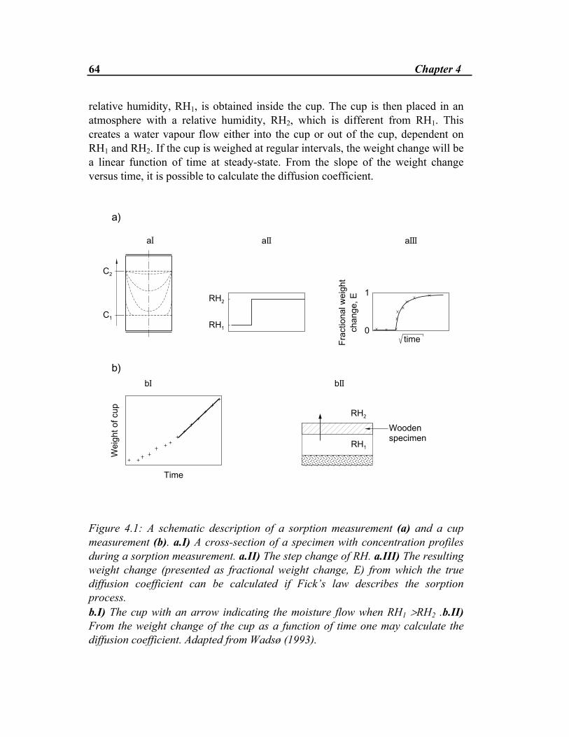
64 Chapter 4
relative humidity, RH1, is obtained inside the cup. The cup is then placed in an atmosphere with a relative humidity, RH2, which is different from RH1. This creates a water vapour flow either into the cup or out of the cup, dependent on RH1 and RH2. If the cup is weighed at regular intervals, the weight change will be a linear function of time at steady-state. From the slope of the weight change versus time, it is possible to calculate the diffusion coefficient.
��
��
���
��� �
�
��
�� �������
�����������
����
��������
�� ���
���
���
����������
��
���������� �
�!
�!
Figure 4.1: A schematic description of a sorption measurement (a) and a cup measurement (b). a.I) A cross-section of a specimen with concentration profiles during a sorption measurement. a.II) The step change of RH. a.III) The resulting weight change (presented as fractional weight change, E) from which the true diffusion coefficient can be calculated if Fick’s law describes the sorption process. b.I) The cup with an arrow indicating the moisture flow when RH1 >RH2 .b.II) From the weight change of the cup as a function of time one may calculate the diffusion coefficient. Adapted from Wadsø (1993).
Diffusion Coefficients 65
In a sorption measurement, the specimen is first equilibrated at an initial relative humidity RH1 until it is at equilibrium with this and shows no weight change. The relative humidity outside the specimen is then rapidly changed to a new value RH2. As wood is hygroscopic the specimen will absorb or desorb water vapour depending on whether RH2 is higher or lower than RH1. This is measured by weighing the specimen at regular intervals. The overall weight change, normally plotted as a function of the square root of time, is most often called a sorption curve, see figure 4.1 a.III. If the material is behaving according to Fick’s law, the diffusion coefficient can be calculated from the initial slope of such a curve. If the moisture transport process is Fickian (i.e., according to Fick’s law) with a constant diffusion coefficient, both methods of obtaining the diffusion coefficient give the same result (Wadsø 1993). The diffusion coefficient for wood however, has shown not to be constant. Over the years many experiments have been done which have shown that the diffusion coefficient, D , for wood is dependent on the driving potential (see e.g., Comstock (1963), Choong and Fogg (1968), Tveit (1966), Kawai (1980), Bertelsen (1984a), Liu Tong (1989), Burch et al. (1992) Wadsø (1993), Time (1995), Vik (1996)).
4.2 Diffusion coefficients evaluated from sorption measurements Equation (3.17), ∂∂
∂∂
Ct x
D dCdxC= ⋅
applies to the non steady-state one-dimensional diffusion in a concentration dependent system, and the solution of this equation is very complex (Comstock (1963), Crank (1975)). However, the general solution for Fick’s second law, equation (3.18),
66 Chapter 4
∂∂
∂
∂
Ct
D C
xC= ⋅
2
2
for a plane sheet with an uniform initial distribution and a step change in surface concentration at t=0, is obtained by use of separation of variables or by a Laplace transformation (Crank 1975):
E tn
n D tl
C
n( )
( )exp ( )
= −+
⋅− +
=
∞
∑1 8 12 1
2 142 2
2 2
20π
π (4.1)
Here E(t) is the fractional weight change as a function of time. The dimensionless sorption E(t)=∆Mt/∆M∞ where ∆Mt is the weight change at time t, and ∆M∞ is the weight change at final equilibrium. l is the half thickness of the specimen. The corresponding solution useful for short periods (not defined any further) is (Crank 1975):
E MM
D tl
ierfc nlD t
t C n
Cn
= = ⋅ + − ⋅
∞ =
∞
∑∆∆
4 1 2 121π( ) (4.2)
For E less than 0.5 the summation term in equation (4.2) becomes negligibly small (Liu Tong 1987) and equation (4.2) can be reduced to:
E MM
D tl
t C= =⋅
∞
∆∆
42
12
π (4.3)
By making a derivation of E in respect to t the following equation is obtained for the diffusion coefficient, DC:
D l Et
l dEd tC =
⋅⋅ =
⋅⋅
π π2 2 2 2
4 4 (4.4)
The diffusion coefficient is determined from the initial stage of an absorption or a desorption curve (E< 0.5).
Diffusion Coefficients 67
This solution of Fick’s second law (equation 3.18) is perhaps the most widely used and it has been used by many researchers throughout the years (Comstock 1963, Choong and Fogg 1968, Absetz et al.1993, Wadsø 1993). This solution of equation (4.2) is subject to the following assumptions (Comstock 1963, Kawai 1980), 1. The moisture is initially uniformly distributed through the specimen. 2. The surface of the specimen immediately reaches the equilibrium
concentration at t > 0. 3. The concentration at the centre of the specimen does not change appreciably. 4. The diffusion coefficient is independent of the concentration in the range
measured. In the final part of the sorption curve, only the first term in equation (4.1) needs to be considered (Crank 1975), and the diffusion coefficient can be expressed as
D lt EC = ⋅
−
4 81
2
2 2π πln
( ) (4.5)
Wadsø (1993) has performed sorption measurements and used both methods of solution, equation 4.4 and 4.5, to evaluate the diffusion coefficient. As a main result he has found that moisture sorption in wood is not fully in accordance with Fick’s law and neither of the solutions will give a true diffusion coefficient. He states that it is impossible to give general recommendations on which method to use, and that the best tactic is probably to use both. All the above mentioned equations give the diffusion coefficient with moisture concentration in wood as the driving potential. Conversion with the aid of a sorption isotherm will be needed if the diffusion coefficient is to be expressed on the basis of water vapour pressure or moisture content in the air. The accuracy of such a recalculation depends on the validity of the sorption isotherm available for the particular wooden material. More recent diffusion coefficients for softwoods evaluated from sorption measurements performed in the Nordic countries are reported. These are, in addition to Wadsø (1993), Liu Tong (1987) and Absetz et al. (1993). Absetz et al. (1993) have done sorption measurements on spruce (Picea abies) and pine (Pinus silvestris) which have been compared with the results presented in Wadsø (1993).
68 Chapter 4
Their conclusion is that the evaluated diffusion coefficients from equation 4.4 compare very well for both spruce and pine when the step change has been nearly equal (i.e., Absetz et al.; 76% to 86% RH, Wadsø (1993); 75% to 84% RH). For the lower step change however, (Absetz et al.; 65% to 76% RH, Wadsø (1993); 54% to 75% RH) the evaluated diffusion coefficients of Wadsø (1993) are about three times larger than those of Absetz et al. (1993). The diffusion coefficients of spruce in a transverse direction (both radial and tangential) reported in Absetz et al. (1993) are in the range of 15 - 30 x10 -12 m2s-1 with a step change in RH between 65% and 86%. A comparative diffusion coefficient from sorption measurements on spruce reported by Liu Tong (1987) is 52 x 10-12 m2/s (step change in RH between 65% and 80%, transverse direction). And the corresponding value for a step change between 65% and 30% RH is 76 x 10-12 m2/s. Liu Tong (1987) has reported a value of 1000 x 10-12 m2s-1 for spruce in the longitudinal direction (step change between 65 and 90% RH). This is in the same area as the longitudinal coefficient for pine reported by Wadsø (1993) although the range of the step change is larger in Liu Tong (1987). One should be aware of that Liu Tong (1987) in the same report discusses diffusion coefficients and thickness effects and presents longitudinal diffusion coefficients evaluated from measurements under approximately the same conditions which varies from 163 x 10-12 m2s-1 (10 mm specimens) to 506 x 10-12 m2s-1 (40 mm specimens).
4.2.1 Absorption versus desorption In contradiction to Liu Tong (1987) and Wadsø (1993), Absetz et al. (1993) have evaluated diffusion coefficients for spruce from both absorption and desorption measurements. They found that diffusion coefficients evaluated from desorption are about three times larger than diffusion coefficients from absorption (radial and tangential direction). Choong and Fogg (1968) have evaluated diffusion coefficients for six different kinds of wood, three hardwoods and three softwoods. For the softwood species with a transport in the radial and the tangential direction an average value of DC-desorption/DC-absorption of 2.5 was found.
Diffusion Coefficients 69
4.2.2 Influence of thickness, heart- versus sapwood and transport direction McNamara and Hart (1971) have reported diffusion coefficients (DC) for the transverse direction of yellow poplar, obtained by the sorption method. The results indicated that the diffusion coefficients tend to decrease with decreasing specimen thickness and with decreasing size of the relative humidity step. Wadsø (1993) has done similar measurements for spruce, and he has also observed that diffusion coefficients (for the transverse direction) obtained for the thinner specimens are lower than those obtained for thicker specimens. The same trend has been reported by Liu Tong (1987) for longitudinal specimens. Results reported by Villadsen et al. (1993), for steady-state cup measurements on pine in the longitudinal direction show the opposite trend. Diffusion coefficients, Dp, for thicker specimens are larger than the corresponding diffusion coefficients for thinner specimens. Absetz et al. (1993) found no unambiguous difference for the diffusion coefficients in the radial and the tangential transport direction in contradiction to Wadsø (1993) who found that radial diffusion is 1.3 times that of tangential. Compared to the fairly large variations in the reported diffusion coefficients for different specimens of wood, this difference in radial and tangential diffusion should have little practical influence for building purposes. From the reported coefficients it can be said that the diffusion in softwoods along the fibres are between 10 and 15 times larger than across the fibres. Liu Tong (1987) and Absetz et al. (1993) both report that no difference in diffusion was found between heartwood and sapwood samples from spruce. They do however, report about differences for pine heartwood versus sapwood.
4.3 Diffusion measurements of spruce by the cup method This chapter starts with a thorough examination of cup measurements performed in this work. The last part of the chapter is devoted to diffusion coefficients of spruce evaluated from cup measurements in general.

70 Chapter 4
4.3.1 Experimental procedure and aspects of the set-up The cup measurements reported here have been performed in two different series in two different experiments. The experiments have been performed in the laboratory at the Department of Building and Construction Engineering and the Norwegian Building Research Institute. A more detailed description of the experiments can be found in Time (1995). Selection of cups Small cups with a diameter of about 80 mm and a depth of 10 - 15 mm have been used. The cups are made from aluminium. The cups are furnished with a protective coating inside to prevent the salt and the aluminium to react chemically. The specimen is mounted as a lid to the cup. See figure 4.2. The reasons for selecting small cups for the experiments were, among others • it is easier to find small specimens without defects • there is less shrinkage and swelling for small specimens • there is less possibility for cracking of the specimens Test method - Principle The experiments have mainly been based on Nordtest method NT Build 130 Edition 2 (NT Build 1990). The principle of a cup measurement is described in chapter 4.1. From the steady-state weight versus time curve, water vapour permeance, diffusion resistance and the diffusion coefficient (often known as water vapour permeability) can be determined. The transfer rate is a function of the difference in vapour pressure, temperature, air velocity above the specimen, air layer thickness below the specimen as well as the specific material properties. Specimens of spruce (Picea abies) The timber used in the experiments is collected at the sawmill, which means that the origin is known. After drying at the sawmill, the spruce samples were brought into the laboratory for preparation of test specimens. Five specimens were taken from one board of spruce for each test. They were all conditioned in an environment with a relative humidity of about 50% and a temperature of 22°C - 23°C until equilibrium was reached (the weight change in 10 days was less than 0.1%). All the specimens were prepared so that the vapour flow was perpendicular to the fibres, in a combined tangential and radial direction. The specimens were taken

Diffusion Coefficients 71
from boards which were sawn from the centre of the timber log, i.e. most likely only heartwood specimens. Sealing of the cups The cup consists of an aluminium frame, in which the specimen is placed, and a cup made from the same material, in which the salt solution is put. The specimen is first sealed around the edge, see figure 4.2, and after that it is sealed to the frame, both sealing compounds consisting of 70% plasticine and 30% bees wax. The frame is then sealed to the cup (same sealing compound). The air gap between the salt solution and the inner surface of the specimen is between 7 - 12 mm, dependent on the height of the frame and the thickness of the specimen.
a) "����� �� "���������� ��
�
�
#� ��� ����
���������
"���������� ��
#� ��� �� �
"������� ���� b) Figure 4.2.: a) Sealing of the specimen, b) Mounting of the test cup
72 Chapter 4
4.3.2 Measurements The test conditions used are described in table 4.1. The test cups were placed in the conditioning room described in chapter 4.3.1 (50% RH and 22°C - 23°C). The water vapour transfer rate through each specimen was determined by weighing the cups every second or third day, until the weight loss/-gain per time was constant. Electronic balances with an accuracy within the range of ± 0.01 gram (Series I) and ± 0.001 gram (Series II) were used. As can be seen from table 4.1 not all cups performed well. If the humidity of the environment inside the cup differed very much from the humidity of the environment outside the cup, the specimen tended to curve across the fibres. The curvature will depend on the difference in the relative humidity across the specimen, the width and the thickness of the specimen. A curved specimen will give a larger exposed area for transmission, the thickness of the air layer inside the cup will vary and the thickness along a specimen may vary. For some specimens the sealing compound could not resist the curving and the sealing was broken. How does this curvature affect the diffusivity of the specimen? Can this be considered in an analysis? The problem with curved specimens has, as far as I am aware of, not been very much discussed in the literature. A reason for this can be that for some of the reported cup measurements the specimen has been put on the cup to get into equilibrium before it is actually sealed to the cup. The specimen will still be curved, but the chances for the sealing to break are reduced. In the calculations of the diffusion coefficient, the specimens have been considered to be un-curved. Joy and Wilson (1965) and Bertelsen (1984a) discuss the effective area for cup measurements and how to calculate the excess water vapour transmission because of the masked edge effects. For thicker specimens the edge mask may present a problem. In addition to the intended vapour path, there are curved paths at the edge, within the masked zone. These paths may result in an excess in the water vapour transmission. Joy and Wilson (1965) present an equation to calculate the relative increase in water vapour transmission. The equation consider the specimen thickness, the width of the masked edge and the test area. According to this way of considering the effective transmission area, my measurements show an approximately 5% too high value in the water vapour transmission (∆G see equation 4.6). This increase in water vapour transmission has not been considered in my calculations of the diffusion coefficient.
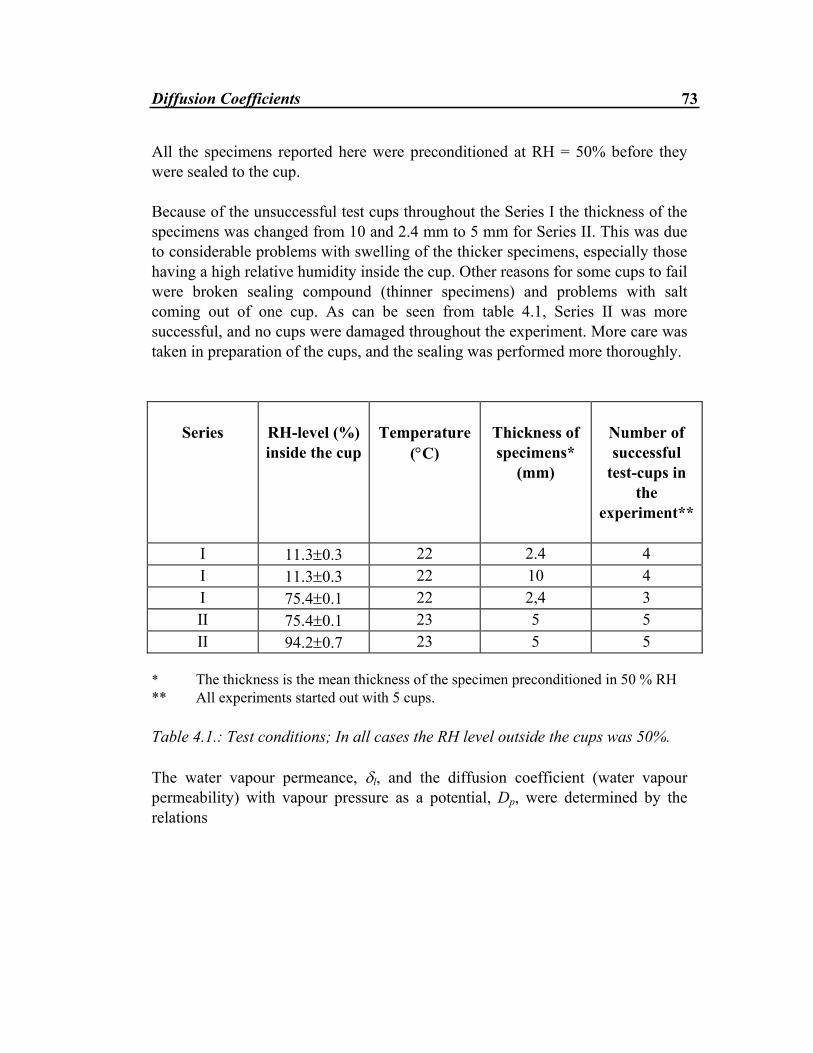
Diffusion Coefficients 73
All the specimens reported here were preconditioned at RH = 50% before they were sealed to the cup. Because of the unsuccessful test cups throughout the Series I the thickness of the specimens was changed from 10 and 2.4 mm to 5 mm for Series II. This was due to considerable problems with swelling of the thicker specimens, especially those having a high relative humidity inside the cup. Other reasons for some cups to fail were broken sealing compound (thinner specimens) and problems with salt coming out of one cup. As can be seen from table 4.1, Series II was more successful, and no cups were damaged throughout the experiment. More care was taken in preparation of the cups, and the sealing was performed more thoroughly.
Series
RH-level (%) inside the cup
Temperature
(°C)
Thickness of specimens*
(mm)
Number of successful
test-cups in the
experiment**
I 11.3±0.3 22 2.4 4 I 11.3±0.3 22 10 4 I 75.4±0.1 22 2,4 3 II 75.4±0.1 23 5 5 II 94.2±0.7 23 5 5
* The thickness is the mean thickness of the specimen preconditioned in 50 % RH ** All experiments started out with 5 cups.
Table 4.1.: Test conditions; In all cases the RH level outside the cups was 50%. The water vapour permeance, δl, and the diffusion coefficient (water vapour permeability) with vapour pressure as a potential, Dp, were determined by the relations

74 Chapter 4
δ l
p
tG
p A Z=
⋅ ⋅ −
1∆∆
∆ (4.6)
D dp l= ⋅δ (4.7) Here ∆G (kg) is the moisture flow during time ∆t (s), ∆p (Pa) is the water vapour pressure difference between the saturated salt solution in the cup and outside the cup, A (m2) is the surface area of the specimen, d (m) is the thickness of the specimen and Zp (Pa⋅m2⋅s⋅kg-1) is the water vapour resistance of the air layer inside the cup. Water vapour resistance of the air layer (Tveit 1966) used an analytical technique to correct his measurements for water vapour resistance of the air layer underneath the sample. He predicted the resistance of the air layer using diffusion theory for a stagnant air layer. The formula can be written as:
Z hTp =⋅ ⋅7 9 10 12
1 3
.,
(4.8)
where h is the thickness of the air layer inside the cup and T is the absolute temperature of the air. The equation has been used in the calculation of the diffusion coefficients evaluated in this work. More details about the given formula are discussed in (Tveit 1966). The water vapour resistance of the surface film has been neglected. Kumaran (1995) has performed a literature review to find out how well one knows the water vapour permeability of stagnant air. He found that the quantity has not yet been precisely determined. But it is clearly established that at 20°C it approaches 2.0⋅10-12 (kg⋅m-1⋅s-1⋅Pa-1). For a 15 mm thick layer of stagnant air at 20°C equation (4.8) gives a ZP = 404⋅106 (Pa⋅m2⋅s⋅kg-1). The corresponding Zp-value calculated from a vapour permeability for stagnant air equal to 2.0⋅10-12 (kg⋅m-1⋅s-1⋅Pa-1) is 75⋅106 (Pa⋅m2⋅s⋅kg-1), more than 5 times less. This might be a reason why Tveit’s values in some comparisons are found rather low (e.g., Nilsson 1990, Villadsen et al. 1993 and Burch et al. 1992).
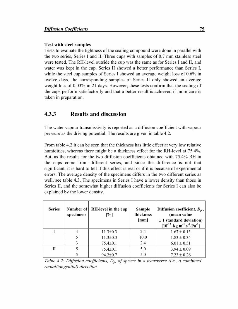
Diffusion Coefficients 75
Test with steel samples Tests to evaluate the tightness of the sealing compound were done in parallel with the two series, Series I and II. Three cups with samples of 0.7 mm stainless steel were tested. The RH-level outside the cup was the same as for Series I and II, and water was kept in the cup. Series II showed a better performance than Series I, while the steel cup samples of Series I showed an average weight loss of 0.6% in twelve days, the corresponding samples of Series II only showed an average weight loss of 0.03% in 21 days. However, these tests confirm that the sealing of the cups perform satisfactorily and that a better result is achieved if more care is taken in preparation.
4.3.3 Results and discussion The water vapour transmissivity is reported as a diffusion coefficient with vapour pressure as the driving potential. The results are given in table 4.2. From table 4.2 it can be seen that the thickness has little effect at very low relative humidities, whereas there might be a thickness effect for the RH-level at 75.4%. But, as the results for the two diffusion coefficients obtained with 75.4% RH in the cups come from different series, and since the difference is not that significant, it is hard to tell if this effect is real or if it is because of experimental errors. The average density of the specimens differs in the two different series as well, see table 4.3. The specimens in Series I have a lower density than those in Series II, and the somewhat higher diffusion coefficients for Series I can also be explained by the lower density.
Series
Number of specimens
RH-level in the cup
[%]
Sample
thickness [mm]
Diffusion coefficient, Dp ,
(mean value ± 1 standard deviation)
[10-12 ⋅kg⋅m-1⋅s-1⋅Pa-1] I 4 11.3±0.3 2.4 1.67 ± 0.13 5 11.3±0.3 10.0 1.83 ± 0.34 3 75.4±0.1 2.4 6.01 ± 0.51
II 5 75.4±0.1 5.0 3.94 ± 0.09 5 94.2±0.7 5.0 7.23 ± 0.26
Table 4.2: Diffusion coefficients, Dp, of spruce in a transverse (i.e., a combined radial/tangential) direction.
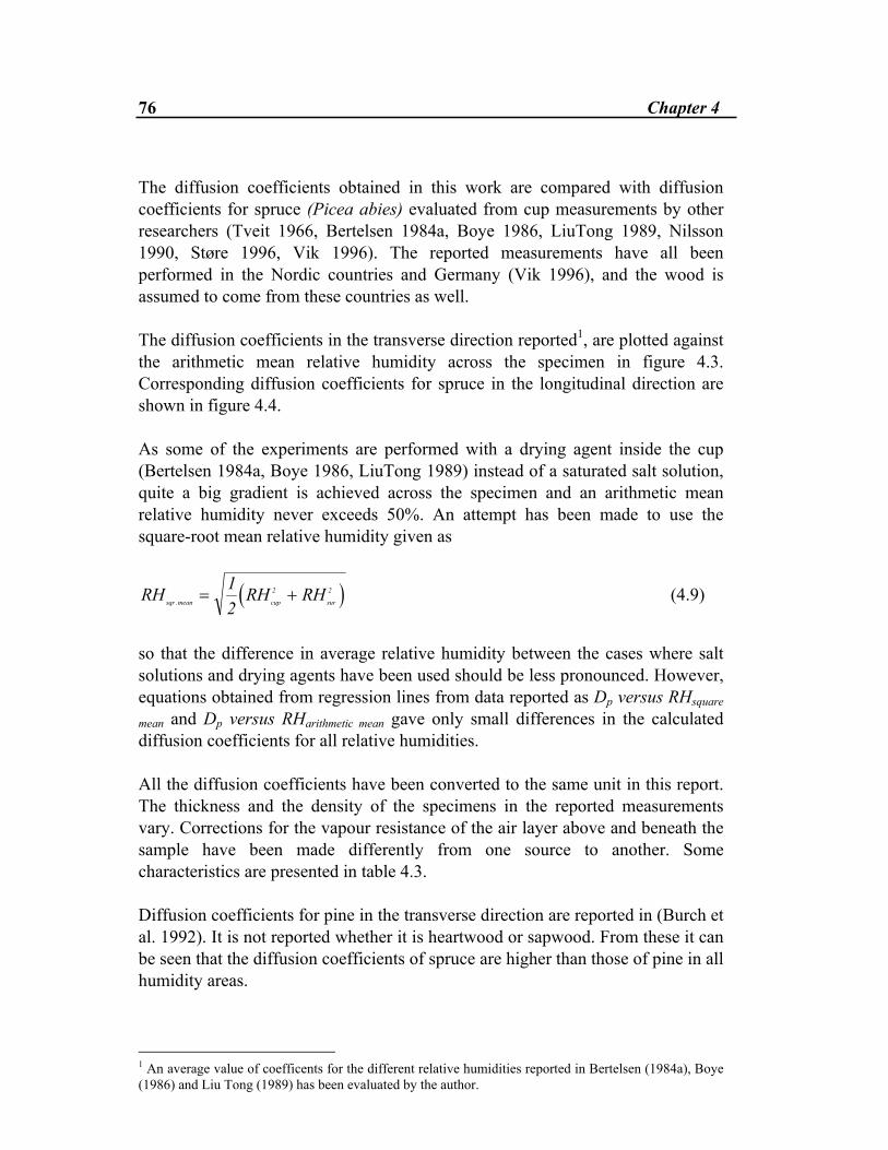
76 Chapter 4
The diffusion coefficients obtained in this work are compared with diffusion coefficients for spruce (Picea abies) evaluated from cup measurements by other researchers (Tveit 1966, Bertelsen 1984a, Boye 1986, LiuTong 1989, Nilsson 1990, Støre 1996, Vik 1996). The reported measurements have all been performed in the Nordic countries and Germany (Vik 1996), and the wood is assumed to come from these countries as well. The diffusion coefficients in the transverse direction reported1, are plotted against the arithmetic mean relative humidity across the specimen in figure 4.3. Corresponding diffusion coefficients for spruce in the longitudinal direction are shown in figure 4.4. As some of the experiments are performed with a drying agent inside the cup (Bertelsen 1984a, Boye 1986, LiuTong 1989) instead of a saturated salt solution, quite a big gradient is achieved across the specimen and an arithmetic mean relative humidity never exceeds 50%. An attempt has been made to use the square-root mean relative humidity given as
( )RH RH RHsqr mean cup sur. = +12
2 2 (4.9)
so that the difference in average relative humidity between the cases where salt solutions and drying agents have been used should be less pronounced. However, equations obtained from regression lines from data reported as Dp versus RHsquare
mean and Dp versus RHarithmetic mean gave only small differences in the calculated diffusion coefficients for all relative humidities. All the diffusion coefficients have been converted to the same unit in this report. The thickness and the density of the specimens in the reported measurements vary. Corrections for the vapour resistance of the air layer above and beneath the sample have been made differently from one source to another. Some characteristics are presented in table 4.3. Diffusion coefficients for pine in the transverse direction are reported in (Burch et al. 1992). It is not reported whether it is heartwood or sapwood. From these it can be seen that the diffusion coefficients of spruce are higher than those of pine in all humidity areas.
1 An average value of coefficents for the different relative humidities reported in Bertelsen (1984a), Boye (1986) and Liu Tong (1989) has been evaluated by the author.
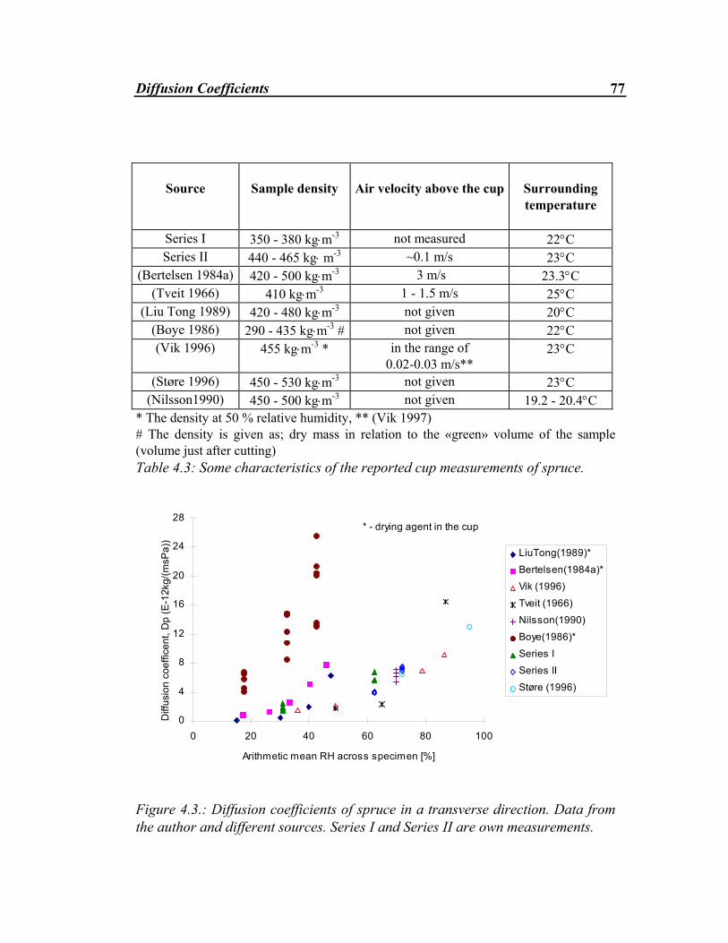
Diffusion Coefficients 77
Source
Sample density
Air velocity above the cup
Surrounding temperature
Series I 350 - 380 kg⋅m-3 not measured 22°C Series II 440 - 465 kg⋅ m-3 ~0.1 m/s 23°C
(Bertelsen 1984a) 420 - 500 kg⋅m-3 3 m/s 23.3°C (Tveit 1966) 410 kg⋅m-3 1 - 1.5 m/s 25°C
(Liu Tong 1989) 420 - 480 kg⋅m-3 not given 20°C (Boye 1986) 290 - 435 kg⋅m-3 # not given 22°C (Vik 1996) 455 kg⋅m-3 * in the range of
0.02-0.03 m/s** 23°C
(Støre 1996) 450 - 530 kg⋅m-3 not given 23°C (Nilsson1990) 450 - 500 kg⋅m-3 not given 19.2 - 20.4°C
* The density at 50 % relative humidity, ** (Vik 1997) # The density is given as; dry mass in relation to the «green» volume of the sample (volume just after cutting) Table 4.3: Some characteristics of the reported cup measurements of spruce.
0
4
8
12
16
20
24
28
0 20 40 60 80 100
Arithmetic mean RH across specimen [%]
Diff
usio
n co
effic
ent,
Dp
(E-1
2kg/
(msP
a))
LiuTong(1989)*
Bertelsen(1984a)*
Vik (1996)
Tveit (1966)
Nilsson(1990)
Boye(1986)*
Series I
Series II
Støre (1996)
* - drying agent in the cup
Figure 4.3.: Diffusion coefficients of spruce in a transverse direction. Data from the author and different sources. Series I and Series II are own measurements.
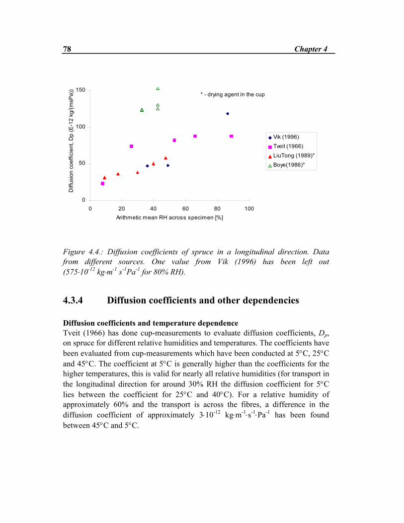
78 Chapter 4
0
50
100
150
0 20 40 60 80 100Arithmetic mean RH across specimen [%]
Diff
usio
n co
effic
ient
, Dp
(E-1
2 kg
/(msP
a))
Vik (1996)
Tveit (1966)
LiuTong (1989)*
Boye(1986)*
* - drying agent in the cup
Figure 4.4.: Diffusion coefficients of spruce in a longitudinal direction. Data from different sources. One value from Vik (1996) has been left out (575⋅10-12 kg⋅m-1 s-1Pa-1 for 80% RH).
4.3.4 Diffusion coefficients and other dependencies Diffusion coefficients and temperature dependence Tveit (1966) has done cup-measurements to evaluate diffusion coefficients, Dp, on spruce for different relative humidities and temperatures. The coefficients have been evaluated from cup-measurements which have been conducted at 5°C, 25°C and 45°C. The coefficient at 5°C is generally higher than the coefficients for the higher temperatures, this is valid for nearly all relative humidities (for transport in the longitudinal direction for around 30% RH the diffusion coefficient for 5°C lies between the coefficient for 25°C and 40°C). For a relative humidity of approximately 60% and the transport is across the fibres, a difference in the diffusion coefficient of approximately 3⋅10-12 kg⋅m-1⋅s-1⋅Pa-1 has been found between 45°C and 5°C.
Diffusion Coefficients 79
Liu Tong (1989) has also reported diffusion coefficients for spruce for different temperatures, 10°C, 20°C, 30°C and 40°C . He has done cup measurements with a drying agent inside the cups and 80% RH at the outside. He found that the coefficients for 10°C and 40°C is slightly lower (approximately 1⋅10-12 kg⋅m-1⋅s-1⋅Pa-1) than for 20°C (approx. 2⋅10-12 kg⋅m-1⋅s-1⋅Pa-1 ) and 30°C (approx. 1.5⋅10-12 kg⋅m-1⋅s-1⋅Pa-1 ). The coefficients for around 20 °C are highest for all samples. Burch (1992) has reported diffusion coefficients, Dp, for sugar pine at 7°C and 25°C for different relative humidities (cup measurements). No significant temperature dependence was found. On the other hand if plotted as diffusion coefficients with moisture concentration in wood as a potential, DC , a significant temperature dependence is found. This is mainly because of the appearance of the vapour saturation pressure in the transformation equation, which differs from one temperature to another. The moisture diffusion coefficients, DC, increase for increasing temperature for all moisture contents. For the conversion of coefficients, see chapter 4.5. Many of the reported moisture-transfer coefficients are reported as diffusion coefficients with moisture concentration in wood as a potential and as functions of moisture concentration in wood. They are both steady-state and transient values. As mentioned earlier, use in wood science moisture concentration is mostly used as a driving potential. Transfer coefficients on such a form are presented in Choong (1963), Comstock (1963), Choong and Fogg (1968), Koponen (1986) and Wadsø (1993). As it is difficult to measure the moisture concentration in the top and the bottom part of a cup specimen directly, a sorption isotherm is needed to evaluate the moisture concentration. Hjort (1991) has presented a method where a thin slice (1 mm thick) piece of wood is removed from the top/bottom of the specimen immediately after finishing the experiment. The slice of wood is weighed and put into a very small tube for measuring the relative humidity. Diffusion coefficients and dependence of density Few reported studies have focused on diffusion coefficients and dependence of density. Several different variables affect the evaluated diffusion coefficients, something which makes a study on the effect of density on diffusion coefficients based on results from different researchers difficult and imprecise. Boye (1986) has done a thorough study on the effect of different genetic factors on the diffusion coefficient (DP) for spruce (Picea abies). The different factors

80 Chapter 4
studied have been; how the tree has been formed (provenances or clones), where it has grown, transport direction, amount of latewood, area of cell-lumens and density of the wood. One of his conclusions is that density is probably the best basis to conclude on whether the wood has a high or a low diffusion coefficient, Dp, no other factors gave any unambiguous dependencies on such relationships. Rydell (1982) has done a study on the influence of the growthring-width and the density on properties which influences on the durability of Swedish pine. One property that has been investigated is the absorption of water vapour from humid air. He concludes that the vapour absorption is slightly slower for specimens of higher density. On the other hand the difference in moisture sorption of heart- and sapwood is just as big as the influence of density. No relationship has been found for growthring-width and moisture sorption. Absetz et al. (1993) have studied the effect of density on diffusion coefficients, DC, evaluated from absorption and desorption measurements (transient measurements). They found that the diffusion coefficients are slightly dependent on the density, the lower density specimens having a higher diffusion coefficient. They have also found that the density has a stronger effect on desorption diffusion coefficients compared to the absorption diffusion coefficients. It seems logical that diffusion coefficients for wood depend, to a certain extent, on density. Density is a measure of the area of cell-lumens and cell-wall respectively. Diffusion through the cell lumens are much faster than diffusion through the cell wall, and in that sense a certain density dependence is to be expected. Liu Tong (1989), has done diffusion measurements (cup measurements) on spruce and pine and concludes that the small variations of the density in spruce and pine do not have a strong effect on the diffusion coefficient. Specimens with a high content of resin and in that sense a higher density on the other hand, had a large reduction in the diffusion coefficient corresponding to half of what had been measured for the other samples.
4.4 Comparison of diffusion coefficients obtained by the two methods Comstock (1963) and Wadsø (1993) are, as far as I am aware of, the only researchers which have done experimental investigations on wood with the
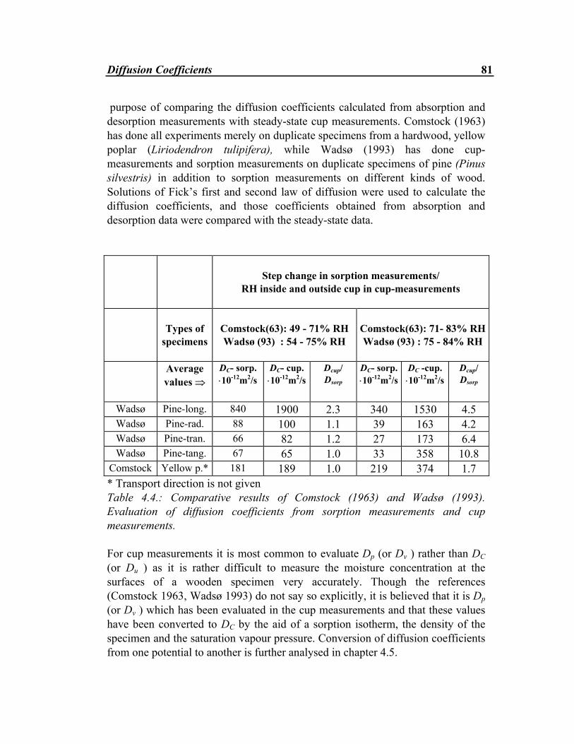
Diffusion Coefficients 81
purpose of comparing the diffusion coefficients calculated from absorption and desorption measurements with steady-state cup measurements. Comstock (1963) has done all experiments merely on duplicate specimens from a hardwood, yellow poplar (Liriodendron tulipifera), while Wadsø (1993) has done cup-measurements and sorption measurements on duplicate specimens of pine (Pinus silvestris) in addition to sorption measurements on different kinds of wood. Solutions of Fick’s first and second law of diffusion were used to calculate the diffusion coefficients, and those coefficients obtained from absorption and desorption data were compared with the steady-state data.
Step change in sorption measurements/
RH inside and outside cup in cup-measurements
Types of
specimens
Comstock(63): 49 - 71% RH Wadsø (93) : 54 - 75% RH
Comstock(63): 71- 83% RHWadsø (93) : 75 - 84% RH
Average
values ⇒
DC- sorp. ⋅10-12m2/s
DC- cup. ⋅10-12m2/s
Dcup/ Dsorp
DC- sorp.⋅10-12m2/s
DC -cup. ⋅10-12m2/s
Dcup/ Dsorp
Wadsø Pine-long. 840 1900 2.3 340 1530 4.5 Wadsø Pine-rad. 88 100 1.1 39 163 4.2 Wadsø Pine-tran. 66 82 1.2 27 173 6.4 Wadsø Pine-tang. 67 65 1.0 33 358 10.8
Comstock Yellow p.* 181 189 1.0 219 374 1.7 * Transport direction is not given Table 4.4.: Comparative results of Comstock (1963) and Wadsø (1993). Evaluation of diffusion coefficients from sorption measurements and cup measurements. For cup measurements it is most common to evaluate Dp (or Dv ) rather than DC (or Du ) as it is rather difficult to measure the moisture concentration at the surfaces of a wooden specimen very accurately. Though the references (Comstock 1963, Wadsø 1993) do not say so explicitly, it is believed that it is Dp (or Dv ) which has been evaluated in the cup measurements and that these values have been converted to DC by the aid of a sorption isotherm, the density of the specimen and the saturation vapour pressure. Conversion of diffusion coefficients from one potential to another is further analysed in chapter 4.5.
82 Chapter 4
In both studies it was found that for lower moisture contents, (i.e. for approximately 11±2 weight %, which corresponds to approximately 70% RH) there was small difference between the coefficients evaluated from the two methods. But at higher moisture contents, diffusion coefficients from both absorption and desorption measurements were well below those obtained from steady-state cup measurements. Comparative results given in Wadsø (1993) and Comstock (1963) are shown in table 4.4. The experiments were performed at a surrounding temperature of 23°C and 40°C respectively. Since the variations of the diffusion coefficients reported in general are quite significant, it is difficult to compare measurements from different researchers. The above comparisons could be done because they were done on the same material, and should, in that sense be directly comparable.
4.5 Conversion of diffusion coefficients For wood it has been found that the two different methods of evaluating diffusion coefficients give different results (see e.g. Comstock 1963, Wadsø 1993). The difference between the coefficients evaluated by the two different methods are thought to be explained by the so called non-Fickian or anomalous behaviours (Wadsø 1993). Non-Fickian behaviours are explained in more detail in Chapter 2. However, to directly be able to compare the diffusion coefficients obtained from the different methods a conversion of the coefficients from one potential to another has to be done. DC (or Du) is the diffusion coefficient evaluated from a non-steady-state (or transient) measurement. DP (or Dv) is the diffusion coefficient evaluated from a steady-state measurement, a cup measurement. In this work a further investigation of the conversion of a steady-state to a non-steady-state (transient) diffusion coefficient has been done. The appropriate conversion equation is (equation 3.10)
Diffusion Coefficients 83
D D puC p
s= ⋅ ⋅ρ ∂
∂ϕ0
1
The saturation pressure, ps , can be evaluated from the temperature at which the experiment has taken place, the dry density, ρ0 , of the specimens have to be known and the moisture capacity, ∂ ∂ϕ
u , should be evaluated from the slope of
the sorption isotherm.
4.5.1 Case-study Diffusion coefficients, DP , for spruce evaluated from measurements performed in this project have been converted into DC . From equation 3.10, the following have to be known to do the conversion; • the temperature during the experiment (to decide the saturation pressure) • the dry density of the material • the first derivative of the sorption isotherm (the moisture capacity) Sorption isotherms and moisture capacity For the most correct results to be obtained, the absorption and desorption isotherm for that particular material have to be known. The first derivative of the isotherms (the slope of the isotherms) represents the moisture capacity of the material and is needed for the conversion. In practice the isotherms (absorption and desorption) for the particular material are very rarely known, and you normally have to make use of sorption isotherms which already exist. Sorption isotherms established experimentally by different researchers have been fitted to the Hailwood and Horrobin equation, which has been found suitable for wood (Skaar 1988, LiuTong 1989, Absetz et al. 1993). The Hailwood and Horrobin equation, with curve-fitting parameters A, B, C, is given as:
uA B C
=+ ⋅ − ⋅
ϕϕ ϕ 2 (4.10)
The derivative of the Hailwood and Horrobin equation, which represents the slope of the sorption isotherm and the moisture capacity, is expressed with the same curve fitting parameters A, B, C as;
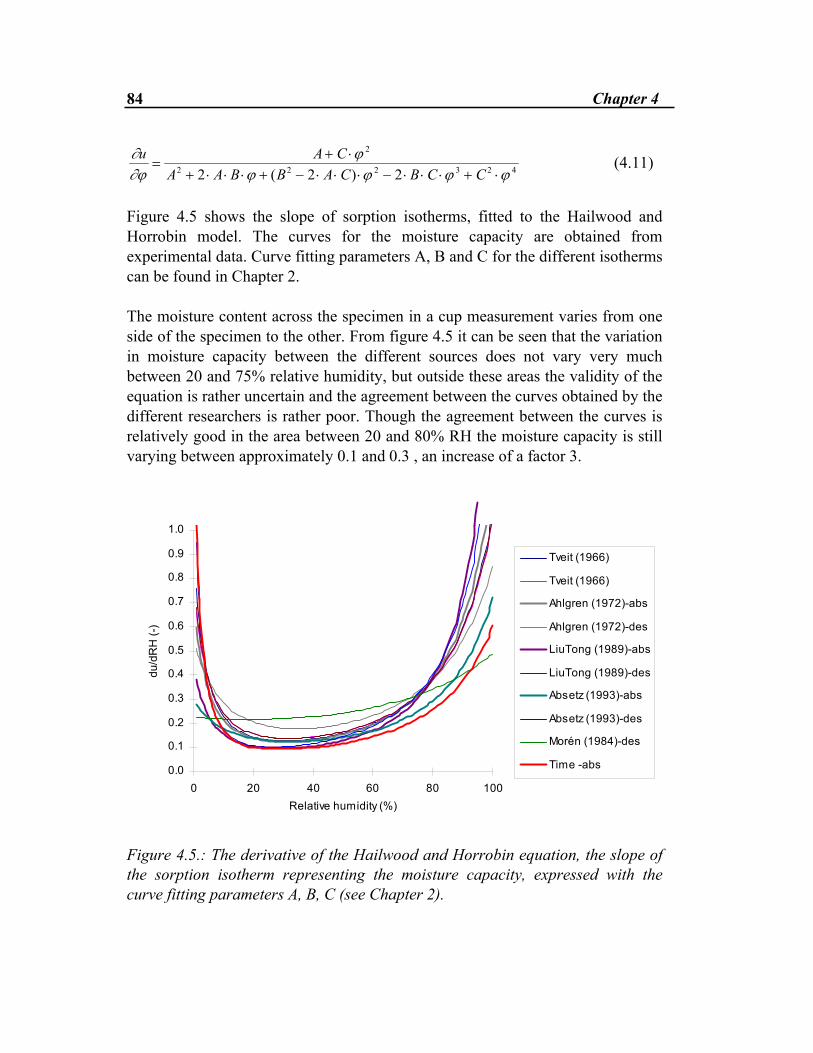
84 Chapter 4
∂∂ϕ
ϕϕ ϕ ϕ ϕ
u A CA A B B A C B C C
=+ ⋅
+ ⋅ ⋅ ⋅ + − ⋅ ⋅ ⋅ − ⋅ ⋅ ⋅ + ⋅
2
2 2 2 3 2 42 2 2( ) (4.11)
Figure 4.5 shows the slope of sorption isotherms, fitted to the Hailwood and Horrobin model. The curves for the moisture capacity are obtained from experimental data. Curve fitting parameters A, B and C for the different isotherms can be found in Chapter 2. The moisture content across the specimen in a cup measurement varies from one side of the specimen to the other. From figure 4.5 it can be seen that the variation in moisture capacity between the different sources does not vary very much between 20 and 75% relative humidity, but outside these areas the validity of the equation is rather uncertain and the agreement between the curves obtained by the different researchers is rather poor. Though the agreement between the curves is relatively good in the area between 20 and 80% RH the moisture capacity is still varying between approximately 0.1 and 0.3 , an increase of a factor 3.
0.0
0.1
0.2
0.3
0.4
0.5
0.6
0.7
0.8
0.9
1.0
0 20 40 60 80 100Relative humidity (%)
du/d
RH
(-)
Tveit (1966)
Tveit (1966)
Ahlgren (1972)-abs
Ahlgren (1972)-des
LiuTong (1989)-abs
LiuTong (1989)-des
Absetz (1993)-abs
Absetz (1993)-des
Morén (1984)-des
Time -abs
Figure 4.5.: The derivative of the Hailwood and Horrobin equation, the slope of the sorption isotherm representing the moisture capacity, expressed with the curve fitting parameters A, B, C (see Chapter 2).

Diffusion Coefficients 85
If the relative humidity inside the cup is 30% and the relative humidity outside is 85%, what will be the correct assumption of moisture capacity for the specimen? Can we assume linear relationship in moisture content between the two sides of the specimen and use the capacity corresponding to the arithmetic mean moisture content? What is the effect of a small variation in temperature on the conversion factor? Diffusion coefficients evaluated at slightly different temperatures are often compared directly. How much is the conversion factor influenced by the dry density of the material? The dry density for wood is varying from species to species and from log to log. The variations in dry density for the more common wood species are between 300 - 800 kg/m3. What does the choice of dry density mean to the conversion factor ? The following chapter focuses on how much the different factors affect the derivation of the diffusion coefficient with moisture concentration in wood as a potential.
4.5.2 Conversion of diffusion coefficients using a 23 factorial experimental design
To evaluate the effects of the three different parameters; saturation pressure (here related to a reported temperature), the dry density of the wood and the moisture capacity (the slope of the sorption isotherm), a 23 factorial design (Box et al. 1978) was set up for the conversion. To perform a general factorial experiment design, an investigator selects a fixed number of “levels” (or “versions”) for each number of variables (factors) and runs experiments with all possible combinations. A 2k factorial design is a design where each variable (factor) occurs at only two levels (e.g., a low level and a high level). Assume that the temperature in the cup measurements reported in this project was uncertain and that the temperature could actually have been 23±2°C. That give us a low temperature of 21°C and a high temperature of 25°C. We can further assume that the dry density could be varying between 350 - 500 kg⋅m-3, which is not unusual for spruce grown in Scandinavia. The low and the high level of the moisture capacity of the material have been set to be corresponding to the relative humidity on either side of the specimen, see table 4.5. An average value of the different curves given in figure 4.5 has been used. The following definition yields
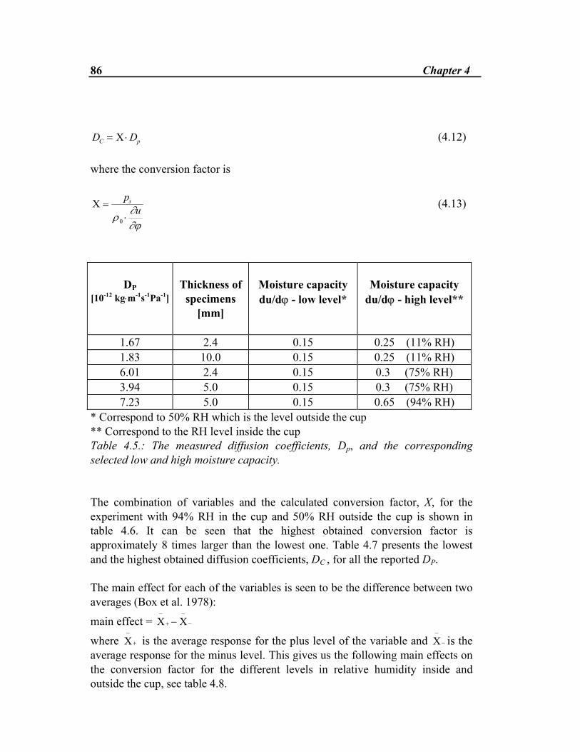
86 Chapter 4
D DC p= ⋅Χ (4.12) where the conversion factor is
Χ =⋅
pu
s
ρ ∂∂ϕ0
(4.13)
DP
[10-12 kg⋅m-1s-1Pa-1]
Thickness of
specimens [mm]
Moisture capacity du/dϕ - low level*
Moisture capacity
du/dϕ - high level**
1.67 2.4 0.15 0.25 (11% RH) 1.83 10.0 0.15 0.25 (11% RH) 6.01 2.4 0.15 0.3 (75% RH) 3.94 5.0 0.15 0.3 (75% RH) 7.23 5.0 0.15 0.65 (94% RH)
* Correspond to 50% RH which is the level outside the cup ** Correspond to the RH level inside the cup Table 4.5.: The measured diffusion coefficients, Dp, and the corresponding selected low and high moisture capacity. The combination of variables and the calculated conversion factor, X, for the experiment with 94% RH in the cup and 50% RH outside the cup is shown in table 4.6. It can be seen that the highest obtained conversion factor is approximately 8 times larger than the lowest one. Table 4.7 presents the lowest and the highest obtained diffusion coefficients, DC , for all the reported DP. The main effect for each of the variables is seen to be the difference between two averages (Box et al. 1978):
main effect = Χ Χ−
+
−
−−
where Χ−
+ is the average response for the plus level of the variable and Χ−
− is the average response for the minus level. This gives us the following main effects on the conversion factor for the different levels in relative humidity inside and outside the cup, see table 4.8.
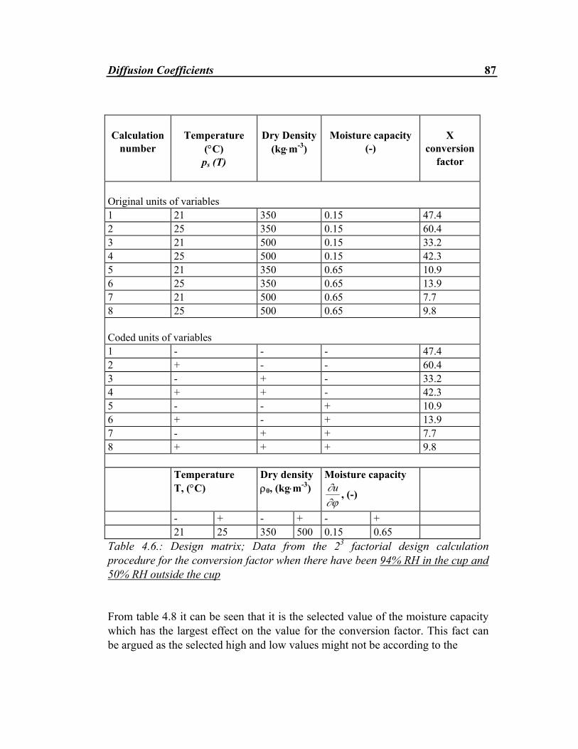
Diffusion Coefficients 87
Calculation number
Temperature
(°C) ps (T)
Dry Density
(kg⋅m-3)
Moisture capacity
(-)
X
conversion factor
Original units of variables 1 21 350 0.15 47.4 2 25 350 0.15 60.4 3 21 500 0.15 33.2 4 25 500 0.15 42.3 5 21 350 0.65 10.9 6 25 350 0.65 13.9 7 21 500 0.65 7.7 8 25 500 0.65 9.8 Coded units of variables 1 - - - 47.4 2 + - - 60.4 3 - + - 33.2 4 + + - 42.3 5 - - + 10.9 6 + - + 13.9 7 - + + 7.7 8 + + + 9.8 Temperature
T, (°C) Dry density ρ0, (kg⋅m-3)
Moisture capacity ∂∂ϕ
u , (-)
- + - + - + 21 25 350 500 0.15 0.65 Table 4.6.: Design matrix; Data from the 23 factorial design calculation procedure for the conversion factor when there have been 94% RH in the cup and 50% RH outside the cup From table 4.8 it can be seen that it is the selected value of the moisture capacity which has the largest effect on the value for the conversion factor. This fact can be argued as the selected high and low values might not be according to the

88 Chapter 4
average value of the moisture capacity that is likely to find across a specimen. The moisture capacity is the most difficult variable to estimate, as it is dependent on moisture content and it is impossible to measure directly. But it can be seen from table 4.5 and 4.7, that also a rather small difference in the high and the low level of the moisture capacity (11-50% RH) can give a high relation between the lowest and the highest obtained diffusion coefficient, DC. The difference between the selected high (0.25) and low (0.15) level is of the same order of magnitude as the difference in moisture capacity presented by the different researchers (figure 4.5).
RH level inside and
outside cup
Thickness
of specimen
(mm)
DP
(10-12⋅ kg⋅m-1⋅s-1⋅Pa-1)
DC
lowest value
(10-12m⋅s-2)
DC
highest value
(10-12m⋅s-2)
DC HIGH/ DC LOW
11-50%RH 2.4 1.67 13 101 8 11-50%RH 10.0 1.83 14 110 8 75-50%RH 2.4 6.01 100 363 4 75-50%RH 5.0 3.94 65 238 4 94-50%RH 5.0 7.23 55 437 8
Table 4.7.: The lowest and highest obtained diffusion coefficients, DC, for the conversion of the coefficients obtained and reported in this thesis.
main effect = Χ Χ−
+
−
−−
RH-level inside and outside the cup
11% - 50%
75% - 50% RH
94% - 50%
Temperature 6.8 8.3 6.8 Dry density -9.9 -12.1 - 9.9
Moisture capacity
-35.2 22.9 35.2
Table 4.8.: The main effects of the different variables for the different RH levels inside and outside the cup.
Diffusion Coefficients 89
4.5.3 Discussion A 23 factorial design has been used to convert a diffusion coefficient from one potential to another. The conversion of the diffusion coefficients made shows that the conversion factor is rather sensitive to changes in the different factors included. From experience we do not always know the absorption and desorption isotherm for the particular material we are interested in, the dry density is not always given, nor the exact temperature, at which the measurements have been performed. This suggests that the difference found in comparing diffusion coefficients obtained by cup measurement (steady-state) and by sorption measurement (non steady-state) might not necessarily be explained by non-Fickian (or anomalous) behaviours alone.

90 Chapter 4
Chapter 5
Sorption Measurements of Spruce Exposed to Cyclic Step Changes in Relative Humidity The main aim of this project has been to study the variation of moisture content in wood exposed to changes in climatic conditions. Experiments have been performed, limited to changes in relative humidity with a constant temperature. Experimental equipment have been designed and built for this purpose and a brief description of the equipment is given. This chapter investigates the results from experimental measurements of moisture sorption in spruce exposed to cyclic step changes in relative humidity.
5.1 Present knowledge Basic research on hygroscopic moisture sorption in wood exposed to cyclic humidity changes is scarce. The wood science society, which does most research on moisture sorption in wood, is very often interested in wood seasoning and drying of wood from the green condition. In building technology and building
92 Chapter 5
physics wood is a part of a structure, and the methods for measuring the moisture conditions in the structure, the wooden parts included, are selected thereafter. This means that there are small opportunities for doing basic investigation on wood as a material. The variations in the surrounding climate (variation of temperature and relative humidity around the wooden parts) and the accuracy of the moisture content measurements (pin electrodes) put a limit to this. Chomcharn and Skaar (1983) have reported results from an investigation on the relationship between moisture sorption in wood, dimensional changes, time and relative humidity. Test specimens from three different hardwood species were exposed to sinusoidally varying relative humidity between 77% and 47% at 25°C for several cycles. Four different cycling periods were used (5.33, 10.67, 16.0 and 25.33 hours). As a main conclusion they found that both moisture and dimensional changes were generally sinusoidal, but lagged behind the imposed relative humidity. The phase lag decreased and the amplitude increased with increasing cycling period. Both responses and phase lags approached repetitive or «steady-state» values as cycling was prolonged. Håkansson (1994, 1995a) has done an extensive experimental investigation on moisture sorption in very small, thin specimens of pine (Pinus sylvestris) exposed to varying step changes in relative humidity at a constant temperature. The time between each step change differs. There is a variation from 2 to approximately 15 days at each time step. Two temperature levels have been considered, 5°C and 21 °C. He has come to the conclusion that parts of the sorption is time-dependent, and because of this the total moisture capacity of wood is not instantaneously accessible. This effect is more pronounced for the experiments at 5°C. Droin-Josserand et al. (1988) have done sorption experiments on wood exposed to changes in relative humidity in order to verify a numerical mathematical model. Specimens of two different thicknesses, 5 mm and 20 mm, with a transverse transport direction were tested. The relative humidity of the atmosphere has been varied with a constant rate of 5% RH per hour , increasing from 55% RH to 80%, thereafter decreasing from 80 to 55% RH. The temperature was kept constant at 30°C. One of the conclusions drawn from the work is that there is a phase lag between the change in moisture content relative to the change in relative humidity. And the maximum moisture content does not correspond with the maximum of relative humidity.
Sorption Measurements of Spruce exposed to Changes in Relative humidity 93
5.2 Experimental set-up A brief description of the experimental set-up is given in this chapter. A more thorough presentation can be found in Time (1996a).
5.2.1 Cyclic measurements Specimens of spruce and some of pine have been exposed to step changes in relative humidity at a constant temperature of 25°C. The weight of the specimens has been measured as a function of time, and an average moisture content evaluated. The measurements which have been performed can be described as four different measurement series. These are; • Series 1: Weekly cycles between 94% and 75% RH, 7 weeks of measurements • Series 2: Daily cycles between 94% and 75% RH, 2 weeks of measurements • Series 3: Daily cycles between 54% and 75% RH, 2 weeks of measurements • Series 4: Weekly cycles between 54% and 75% RH, 7 weeks of measurements The temperature and the relative humidity of the air surrounding the specimens have been logged. Saturated salt solutions have been used to achieve the different relative humidities. The measured step changes, the salt characteristics and experiences with the measurements are presented in Appendix 5.A. Sources of inaccuracies in the measurements have been present. The most important are : • the accuracy of the salt solutions • the accuracy of the different sensors • the accuracy of the balance. A so called «blind specimen» of stainless steel has
been weighed together with the wooden specimens throughout all measuring series to control the weighings. This reference specimen has been sealed with the same vapour tight polyethylene tape and the same stainless steel hook as for the test specimens.
• the temperature fluctuations in the room where the sorption apparatus is stored. • the influence of the room air on the test specimens for about 30 - 60 seconds
when changing the vessels.

94 Chapter 5
• disturbances in the climate in the vessel during weighing (minor effects
compared to the other points)
5.2.2 Description of sorption equipment The sorption equipment, also named as an sorption apparatus, have been designed and built for the purpose of this project. The apparatus consists of two thin walled cylindrical polyethylene vessels with a diameter of 80 cm and a height of about 90 cm, see figure 5.1 to 5.3. The two vessels have different relative humidity inside. Shallow trays containing saturated salt solutions are placed in the bottom of each vessel to provide a given relative humidity. A construction containing the test specimens and a fan performs as the top of one vessel at a time, see figure 5.1 to 5.3. The construction consists of a cylindrical polyacrylic plastic slab with a PVC tube in the middle. The PVC tube is hanging on the slab, still it is possible to turn the tube. Rigid steel wires, on which to hang the test specimens, are fastened symmetrically around the tube. Inside the tube there is a fan which makes the air circulate through the tube, passing by the specimens on the outside. The top construction can be mechanically lifted from one vessel to the other, so that the specimens cyclically get into two different environments. The test specimens get in contact with the ambient air for a very short time only. The weight change of the test specimens is measured as a function of time. A PM 400 electronic precision balance from Mettler is being used. The readability range is from 0 to 400 g with a precision of 1 mg. The balance is placed on the top construction, and the scale of the balance is suspended in a thin, rigid metal wire which is led through the polyacrylic plastic slab. The weighing of the specimens is done by moving them from their hanging position to the suspended hook below the balance. The balance has a fixed position on the top construction. By turning the PVC tube the specimens get into the right position for weighing. The moving of the specimens is done by putting ones hand through a flexible opening in the vessel. The opening is being closed as soon as the hand is taken out. The vessels are placed in a room with a fixed temperature of 23°C. The vessels are without any heat sources and insulation. However, some heat are developed due to the moving blades of the fan, and heat from the fan engine placed on top of
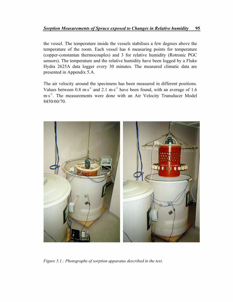
Sorption Measurements of Spruce exposed to Changes in Relative humidity 95
the vessel. The temperature inside the vessels stabilises a few degrees above the temperature of the room. Each vessel has 6 measuring points for temperature (copper-constantan thermocouples) and 3 for relative humidity (Rotronic PGC sensors). The temperature and the relative humidity have been logged by a Fluke Hydra 2625A data logger every 30 minutes. The measured climatic data are presented in Appendix 5.A. The air velocity around the specimens has been measured in different positions. Values between 0.8 m⋅s-1 and 2.1 m⋅s-1 have been found, with an average of 1.6 m⋅s-1. The measurements were done with an Air Velocity Transducer Model 8450/60/70.
Figure 5.1.: Photographs of sorption apparatus described in the text.

96 Chapter 5
�����������
���� ����������������
��������������
�����
������� ����
Figure 5.2.: Sketch of the apparatus, described in the text.
5.2.3 Test specimens The wood used in this experiment has a known past history. The wood is mainly spruce (Picea abies) and some pine (Pinus sylvestris) sawn and collected at sawmills in central Norway. Some of the wood have been dried in an industrial drier, while the rest of it have been dried in room temperature in the laboratory before being used in the experiments. Before the first experiment started (Series 1), all the specimens have been preconditioned until equilibrium were reached (the weight change in 10 days was less than 0.1 %). The environment had a relative humidity of 50% and a temperature of 23°C.
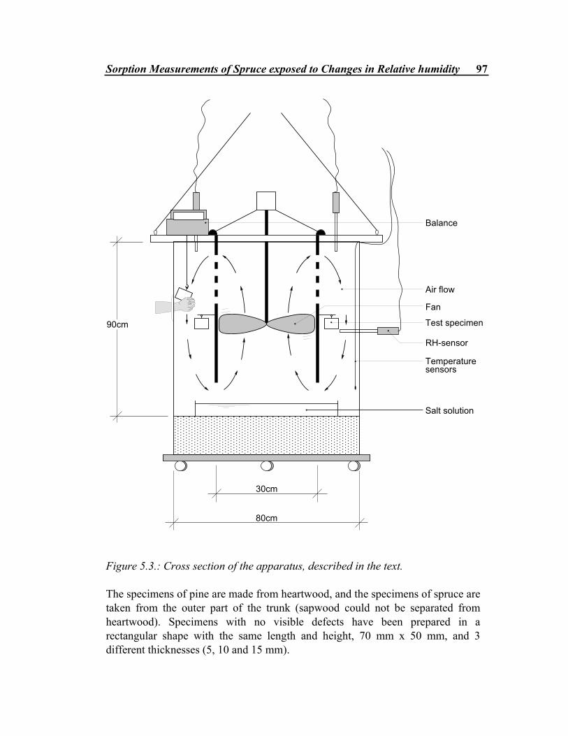
Sorption Measurements of Spruce exposed to Changes in Relative humidity 97
�������
��������
���
�������������
���������
�������� ���������
�������� ����
� ��
! ��
" ��
Figure 5.3.: Cross section of the apparatus, described in the text. The specimens of pine are made from heartwood, and the specimens of spruce are taken from the outer part of the trunk (sapwood could not be separated from heartwood). Specimens with no visible defects have been prepared in a rectangular shape with the same length and height, 70 mm x 50 mm, and 3 different thicknesses (5, 10 and 15 mm).
98 Chapter 5
A one-dimensional water vapour transport was to be achieved and the edges were sealed. The sealing consisted of 3 layers of a very vapour tight polyethylene tape. The dry density of each specimen has been measured. The average dry density of the spruce specimens was 390 kg⋅m-3, and of pine 445 kg⋅m-3. The standard deviation for both spruce and pine were ± 9 kg⋅m-3.
5.3 Results from measurements The main results from the four different series are plotted as an average moisture content by weight (%) versus time (hours) in this chapter. A selection, representing the average results for each kind of specimens, can be seen in figure 5.4 to 5.13. The curves in absorption and desorption for specimens with both transverse and longitudinal transport direction are rather similar in shape. It also seems as if a repetitive «steady-state cycle» is reached rather fast, to a certain degree dependent on immediate past history.
5.3.1 Series 1, weekly step changes between 75% and 94% RH The results are presented in figure 5.4 and 5.5. The curves in absorption and desorption are rather similar. In both absorption and desorption there is a clear limit between the fast sorption and the slow sorption. But it seems as if the moisture change in desorption is slightly faster than in absorption in the first fast stage of the process, while the opposite is the case in the more slow second stage, see also figure 5.19. This effect is also seen for the weekly step cycles in Series 4 (54% to 75% RH), described in section 5.3.4. Certain disturbances in the rather smooth cyclic sorption curves do exist. An abrupt decrease in relative humidity during the first cycle in absorption (after 300 hours) results in a decrease in moisture content for all specimens. The relative humidity change during that drop had an absolute value of 5% in 10 hours, and the average moisture content for the 5 mm specimens changed as much as 2 weight %, figure 5.5. The measured values stabilise thereafter on the same level as before the drop. Some disturbances in RH after approximately 650 hours have resulted in a more pronounced slow second stage of desorption for cycle 2.
Sorption Measurements of Spruce exposed to Changes in Relative humidity 99
As expected, the sorption is faster in the longitudinal direction. On the other side, the difference between the transverse and the longitudinal direction is not that significant and the shape of the curves is very similar. The fast sorption has come to an end after less than 2 days for 10 mm specimens with a radial transport direction and some time less for specimens with a longitudinal transport direction. The average moisture content level for a 10 mm specimen after 2 days in a surrounding of about 90% RH is about 20% (94% RH is not actually reached). From the figures it looks as if the moisture equilibrium in absorption for 94% RH is reached within 3 to 4 days. In desorption it seems to take a little longer time, but equilibrium seems to be reached within the last day before the step change. This might not be the case according to former research (Christensen 1965, Wadsø 1993), but the sorption might have come to a very slow stage indeed. There is not much difference in the sorption process between specimens of 5 mm and 10 mm. Only 5 mm specimens cut so that the transport direction is longitudinal have been used. From figure 5.4 and 5.5 it can be seen that the 5 mm specimens stabilise 1 weight % below in absorption, than the 10 mm specimens. The reason for this is most likely that the 10 mm specimens with a longitudinal transport direction are from the group of specimens with the highest standard deviation (in moisture content), see table 5.1, and the difference may be due to differences between different specimens.
5.3.2 Series 2, daily step changes between 75% and 94% RH Weekly step changes in Series 1 were followed by daily step changes. Results from the measurements are presented in figure 5.6. The sorption process is rather similar to the first part of the process in Series 1, and nearly the same levels of moisture content have been reached after 24 hours as after 1 week. After 1 day and night of sorption the average moisture content level has reached between 19 and 20 %, depending on thickness and direction of transport. The absolute average moisture gain/loss during one day is between 2.5 and 3 weight %. There is no visible difference between absorption and desorption. The shape of the curves is not very smooth in the slower sorption region. This is due to lack of measuring points during the night. Between 120 and 150 hours, and 250 and 310 hours there have not been any weighings. The last cycle represents 3 days of absorption and 1 day of desorption (see last part of figure 5.6). From that we can see that the major part of the sorption happens within the first day, as the
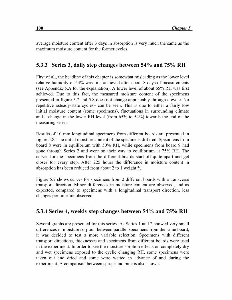
100 Chapter 5
average moisture content after 3 days in absorption is very much the same as the maximum moisture content for the former cycles.
5.3.3 Series 3, daily step changes between 54% and 75% RH First of all, the headline of this chapter is somewhat misleading as the lower level relative humidity of 54% was first achieved after about 8 days of measurements (see Appendix 5.A for the explanation). A lower level of about 65% RH was first achieved. Due to this fact, the measured moisture content of the specimens presented in figure 5.7 and 5.8 does not change appreciably through a cycle. No repetitive «steady-state cycles» can be seen. This is due to either a fairly low initial moisture content (some specimens), fluctuations in surrounding climate and a change in the lower RH-level (from 65% to 54%) towards the end of the measuring series. Results of 10 mm longitudinal specimens from different boards are presented in figure 5.8. The initial moisture content of the specimens differed. Specimens from board 8 were in equilibrium with 50% RH, while specimens from board 9 had gone through Series 2 and were on their way to equilibrium at 75% RH. The curves for the specimens from the different boards start off quite apart and get closer for every step. After 225 hours the difference in moisture content in absorption has been reduced from about 2 to 1 weight %. Figure 5.7 shows curves for specimens from 2 different boards with a transverse transport direction. Minor differences in moisture content are observed, and as expected, compared to specimens with a longitudinal transport direction, less changes per time are observed.
5.3.4 Series 4, weekly step changes between 54% and 75% RH Several graphs are presented for this series. As Series 1 and 2 showed very small differences in moisture sorption between parallel specimens from the same board, it was decided to test a more variable selection. Specimens with different transport directions, thicknesses and specimens from different boards were used in the experiment. In order to see the moisture sorption effects on completely dry and wet specimens exposed to the cyclic changing RH, some specimens were taken out and dried and some were wetted in advance of and during the experiment. A comparison between spruce and pine is also shown.

Sorption Measurements of Spruce exposed to Changes in Relative humidity 101
10
11
12
13
14
15
16
17
18
19
20
21
22
0 200 400 600 800 1000 1200 1400Time [hours]
u - w
eigh
t %
R10
R10
L10
L10
Figure 5.4.: Series 1; Measured moisture content of 10 mm spruce specimens versus time (hours). Longitudinal (L) and radial ( R) transport direction.
10
11
12
13
14
15
16
17
18
19
20
21
22
0 200 400 600 800 1000 1200 1400
Time [hours]
u - w
eigh
t %
L5
L5
L5
L5
Figure 5.5.: Series 1; Measured moisture content of 5 mm spruce specimens versus time (hours). Longitudinal (L) transport direction.
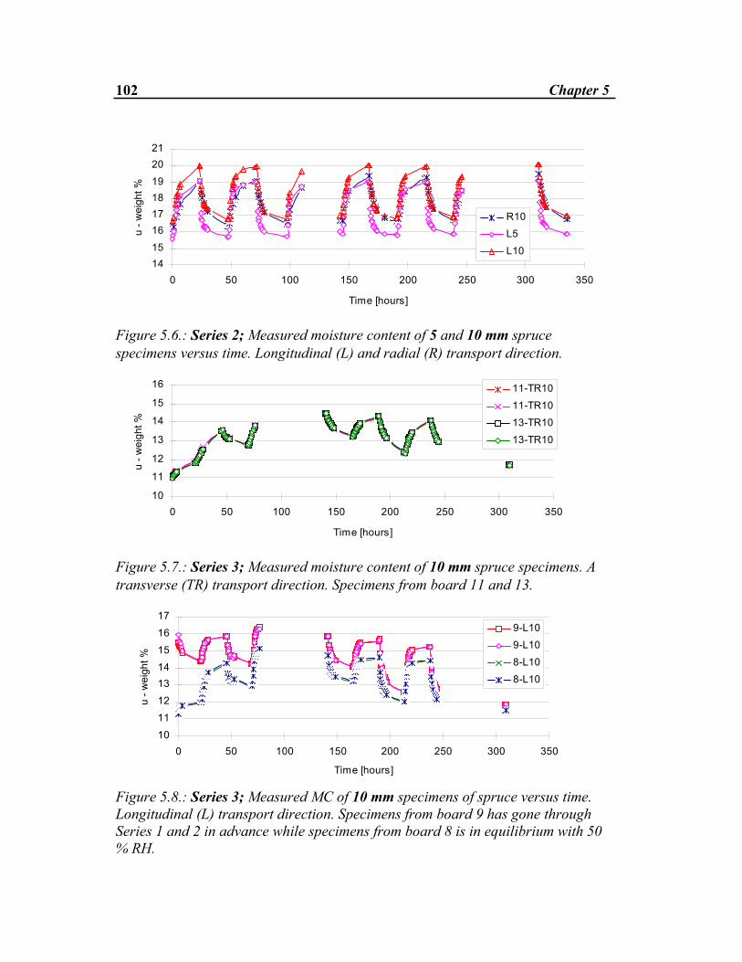
102 Chapter 5
1415
16171819
2021
0 50 100 150 200 250 300 350
Time [hours]
u - w
eigh
t %
R10
L5
L10
Figure 5.6.: Series 2; Measured moisture content of 5 and 10 mm spruce specimens versus time. Longitudinal (L) and radial (R) transport direction.
10
11
12
13
14
15
16
0 50 100 150 200 250 300 350
Time [hours]
u - w
eigh
t %
11-TR10
11-TR10
13-TR10
13-TR10
Figure 5.7.: Series 3; Measured moisture content of 10 mm spruce specimens. A transverse (TR) transport direction. Specimens from board 11 and 13.
10
11
12
1314
15
16
17
0 50 100 150 200 250 300 350
Time [hours]
u - w
eigh
t %
9-L10
9-L10
8-L10
8-L10
Figure 5.8.: Series 3; Measured MC of 10 mm specimens of spruce versus time. Longitudinal (L) transport direction. Specimens from board 9 has gone through Series 1 and 2 in advance while specimens from board 8 is in equilibrium with 50 % RH.
Sorption Measurements of Spruce exposed to Changes in Relative humidity 103
Moisture content versus time for 10 mm specimens is shown in figure 5.9. Through the first cycle, all the moisture content-curves increase smoothly towards an apparent equilibrium value. According to Wadsø (1993), only about 90% of the total weight increase should have been obtained within a week for a transverse specimen of 10 mm thickness for a RH step change between 54% and 75%. However, in this experiment all the specimens seem to have reached equilibrium within a week. The second step change in absorption has resulted in a peak value of nearly 80% RH, see figure 5.A4 in Appendix 5.A. For the 10 mm specimens with a longitudinal transport direction and the 5 mm specimens with both longitudinal and transverse transport direction, the effect of this can be seen, with no time lag, as a corresponding peak in average moisture content. This peak is on the other hand not present for the 10 mm specimen with the transport in a transverse direction, see figure 5.9 and 5.10. Towards the end of the 75% level in the second step of absorption, there is a slight drop and a following rise in relative humidity. A decrease in moisture content can be seen for all specimens in the middle of the 75% level, but a gain in moisture content is not visible for the longitudinal specimens and the thinner transverse specimens at the end of the 75% level. This may be due to fluctuations in RH which have not been registered by the logger (logging every 30 min.). The smaller peaks in RH on the following levels seem to have a slight effect on the thinner specimens, but hardly any effect on the thicker specimens. The moisture content for all specimens seems to reach the same level during all cycles. This is also the case for Series 1, step cycles between 75% and 94%. Comparison of the specimens which have been soaked in water in advance of the experiment and those who have not are shown in figure 5.11. Some specimens were immersed in water when the experiment started. They were put back into the sorption apparatus after one week. The figure shows that the wetted specimens gain more moisture than the drier specimens. They also loose more moisture (in an absolute value) and stable on a moisture content somewhat higher than the drier specimens. It looks as if the difference in moisture content on the upper level slightly decreases from one cycle to another, and the difference in moisture content might disappear after some time. The difference in moisture content at the lower level is not that significant and is about the same from one cycle to another.
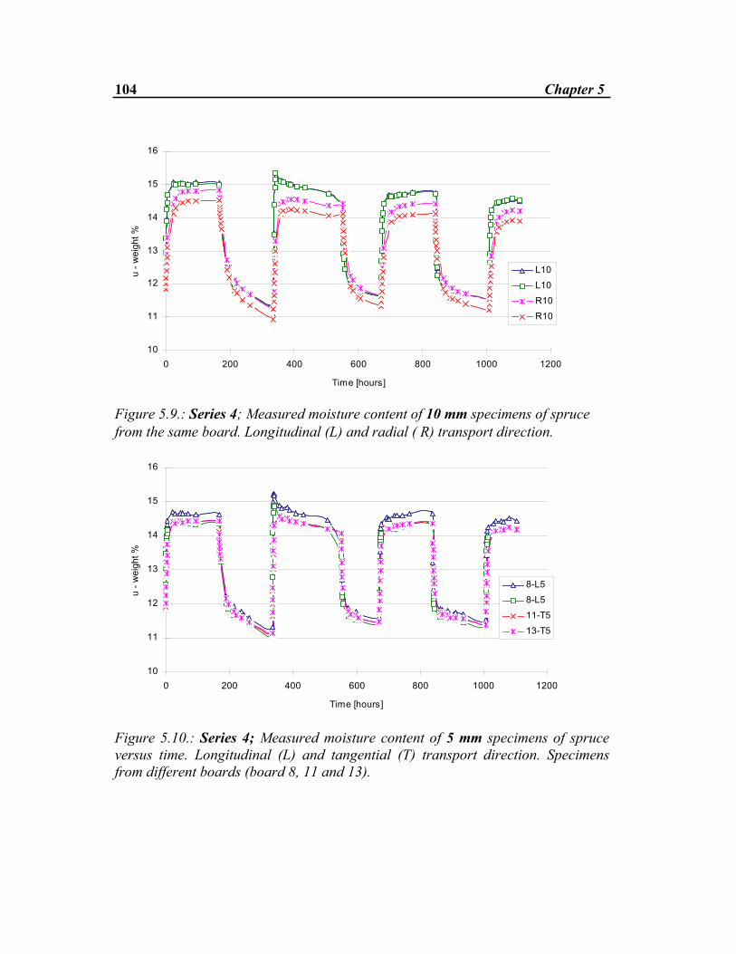
104 Chapter 5
10
11
12
13
14
15
16
0 200 400 600 800 1000 1200
Time [hours]
u - w
eigh
t %
L10
L10
R10
R10
Figure 5.9.: Series 4; Measured moisture content of 10 mm specimens of spruce from the same board. Longitudinal (L) and radial ( R) transport direction.
10
11
12
13
14
15
16
0 200 400 600 800 1000 1200
Time [hours]
u - w
eigh
t %
8-L5
8-L5
11-T5
13-T5
Figure 5.10.: Series 4; Measured moisture content of 5 mm specimens of spruce versus time. Longitudinal (L) and tangential (T) transport direction. Specimens from different boards (board 8, 11 and 13).
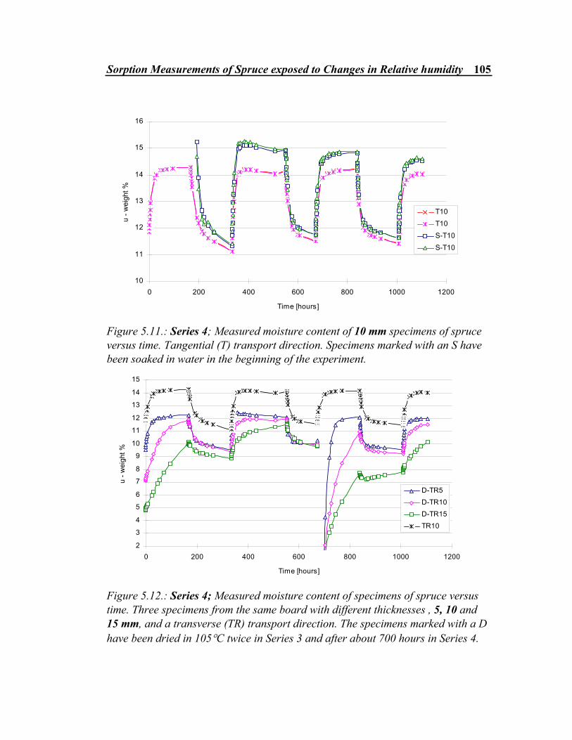
Sorption Measurements of Spruce exposed to Changes in Relative humidity 105
10
11
12
13
14
15
16
0 200 400 600 800 1000 1200
Time [hours]
u - w
eigh
t %
T10
T10
S-T10
S-T10
Figure 5.11.: Series 4; Measured moisture content of 10 mm specimens of spruce versus time. Tangential (T) transport direction. Specimens marked with an S have been soaked in water in the beginning of the experiment.
2
3
4
5
6
7
8
9
10
11
12
13
14
15
0 200 400 600 800 1000 1200
Time [hours]
u - w
eigh
t %
D-TR5
D-TR10D-TR15
TR10
Figure 5.12.: Series 4; Measured moisture content of specimens of spruce versus time. Three specimens from the same board with different thicknesses , 5, 10 and 15 mm, and a transverse (TR) transport direction. The specimens marked with a D have been dried in 105°C twice in Series 3 and after about 700 hours in Series 4.
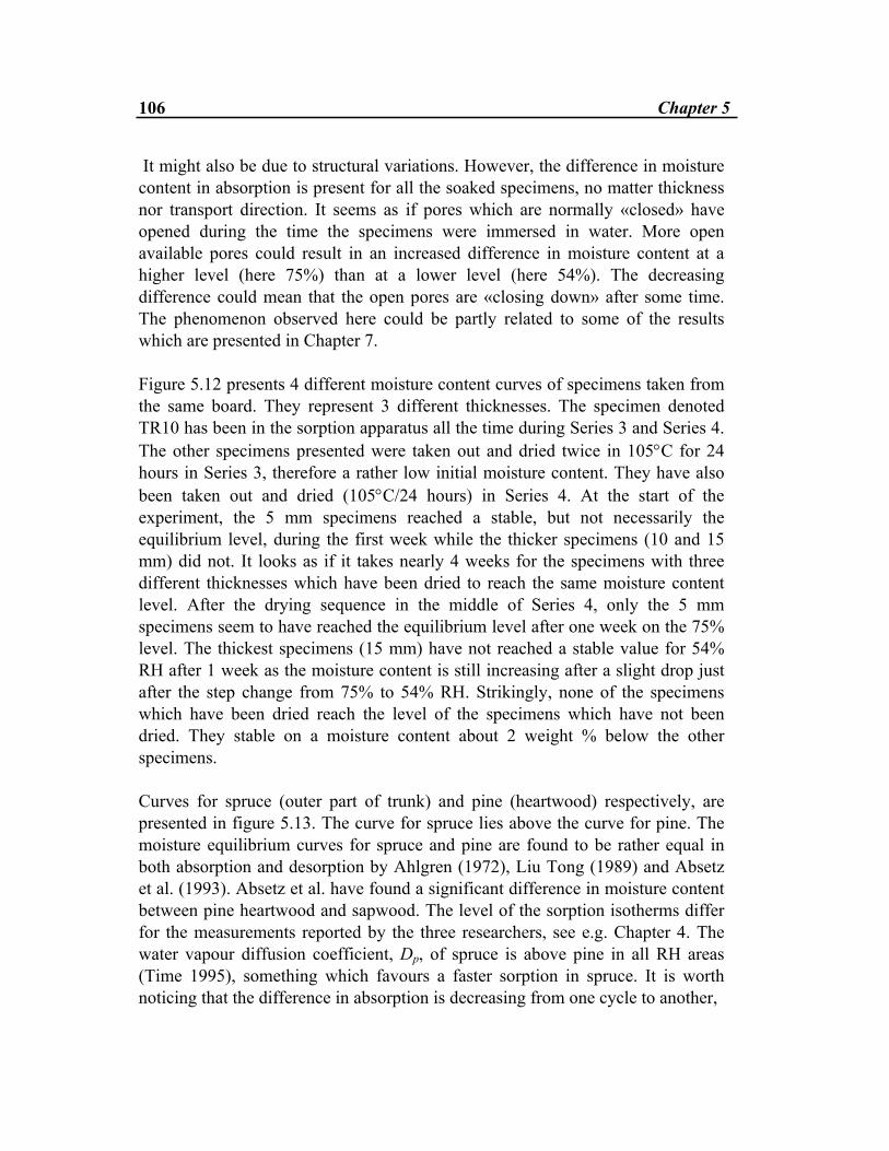
106 Chapter 5
It might also be due to structural variations. However, the difference in moisture content in absorption is present for all the soaked specimens, no matter thickness nor transport direction. It seems as if pores which are normally «closed» have opened during the time the specimens were immersed in water. More open available pores could result in an increased difference in moisture content at a higher level (here 75%) than at a lower level (here 54%). The decreasing difference could mean that the open pores are «closing down» after some time. The phenomenon observed here could be partly related to some of the results which are presented in Chapter 7. Figure 5.12 presents 4 different moisture content curves of specimens taken from the same board. They represent 3 different thicknesses. The specimen denoted TR10 has been in the sorption apparatus all the time during Series 3 and Series 4. The other specimens presented were taken out and dried twice in 105°C for 24 hours in Series 3, therefore a rather low initial moisture content. They have also been taken out and dried (105°C/24 hours) in Series 4. At the start of the experiment, the 5 mm specimens reached a stable, but not necessarily the equilibrium level, during the first week while the thicker specimens (10 and 15 mm) did not. It looks as if it takes nearly 4 weeks for the specimens with three different thicknesses which have been dried to reach the same moisture content level. After the drying sequence in the middle of Series 4, only the 5 mm specimens seem to have reached the equilibrium level after one week on the 75% level. The thickest specimens (15 mm) have not reached a stable value for 54% RH after 1 week as the moisture content is still increasing after a slight drop just after the step change from 75% to 54% RH. Strikingly, none of the specimens which have been dried reach the level of the specimens which have not been dried. They stable on a moisture content about 2 weight % below the other specimens. Curves for spruce (outer part of trunk) and pine (heartwood) respectively, are presented in figure 5.13. The curve for spruce lies above the curve for pine. The moisture equilibrium curves for spruce and pine are found to be rather equal in both absorption and desorption by Ahlgren (1972), Liu Tong (1989) and Absetz et al. (1993). Absetz et al. have found a significant difference in moisture content between pine heartwood and sapwood. The level of the sorption isotherms differ for the measurements reported by the three researchers, see e.g. Chapter 4. The water vapour diffusion coefficient, Dp, of spruce is above pine in all RH areas (Time 1995), something which favours a faster sorption in spruce. It is worth noticing that the difference in absorption is decreasing from one cycle to another,

Sorption Measurements of Spruce exposed to Changes in Relative humidity 107
while the difference in desorption seems constant. Part of the difference is likely due to internal differences in the wood species, but part of it may be due to differences in the sorption process.
10
11
12
13
14
15
16
0 200 400 600 800 1000 1200
Time [hours]
u - w
eigh
t % R10
R10
Pine R10Pine R10
Spruce
Pine
Figure 5.13.: Series 4; Measured moisture content of 10 mm specimens from spruce and pine versus time. Radial ( R) transport direction.
5.4 Variations within the measuring series Many parallel specimens from the same board were chosen in Series 1 (weekly measurements between 75% and 94% RH) and Series 2 (daily measurements between 75% and 94% RH) to study the variations within a limited area of a wooden board. Since the standard deviation between specimens was rather small in Series 1 and 2, not that many parallel specimens were used in Series 3 and 4. Specimens from different boards were used instead. From table 5.1 it can be seen that the average standard deviation in moisture content within a group (same thickness and transport direction) has not increased although specimens from different boards have been used. The group of specimens consisting of both tangential specimens and radial specimens shows a small average standard deviation. This might indicate that there is little difference in the diffusion process between the two transport directions.

108 Chapter 5
Step cycles/Series Weekly 75% - 54% RH
Series 4 Weekly 75% - 94 % RH
Series 1 Type of specimens T/R1
0 TR15 L5 L10 R10 L5 L10
Number of specimens 8* 4* 4 5 10 5 7 Average standard
deviation (moisture content %)
±0.13
±0.09
±0.47
±0.39
±0.34
±0.08
±1.03**
* The specimens are taken from 3 (T/R10) and 2 (TR15) different boards ** The large value is mainly caused by 1 specimen differing from the other 6 Table 5.1.: Number of specimens and the average standard deviation in moisture content, u, for specimens of same thickness and transport direction. Type of specimen codes give moisture transfer direction (TR is combined radial/tangential, T/R are both radial and tangential specimens, R is radial and L is longitudinal) and specimen thickness in mm.
5.5 Influence of surface area on moisture sorption An examination of the effect of the difference in surface area of sorption has been done. This was done to see if this could reduce the average standard deviation. The examination has been done for Series 1 and 2 because this is the series with most parallel specimens within a group. To make the «u - values» comparable to the «u/surface area values», these dimensionless expressions have been used;
uu
usurface area
(usurface area)
average
average
No reduction in standard deviation within a group was found when the surface area was taken into account. The opposite tendency was found. The standard deviation for the moisture content/surface area was slightly higher than for the moisture content values, see table 5.2. There is no reasonable explanation to this,

Sorption Measurements of Spruce exposed to Changes in Relative humidity 109
and it is probably due to casualties. Anyway, the standard deviation is rather small for all groups of specimens.
Average standard deviation within a group
Step cycles/Series Weekly 75% - 94% Series 1
Daily 75% - 94% Series 2
Type of specimens
R10 L5 L10 R 10 L5 L10
Number of specimens
(from the same board)
10
4
6
10
4
7
u/ uaverage
± 0,021 ± 0,050 ± 0,067 ± 0,021 ± 0,021 ± 0,024
(u/surface area)/ (u/surface area)average
± 0,024
± 0,021
± 0,095
± 0,037
± 0,022
± 0,058
Table 5.2.: Average standard deviation within different groups of parallel specimens. Comparison of moisture content (u) and moisture content (u)/surface area.
5.6 Hysteresis and slow sorption
5.6.1 Influence of hysteresis Specimens in Series 1 reached the 75% RH level in desorption, while specimens in Series 4 reached the same level in absorption. A combined influence of hysteresis and slow sorption can be seen in figure 5.14. The results for some specimens from the two weekly series, Series 1 and 4, are presented. The initial moisture content for the specimens of Series 1 was in equilibrium with a surrounding RH of 50%, while the initial moisture content for specimens of Series 4 was the corresponding moisture content at the end of Series 3 (daily step changes between 54% and 75% RH). This is the reason why the result from Series 1 is below the result from Series 3 in the initial part.
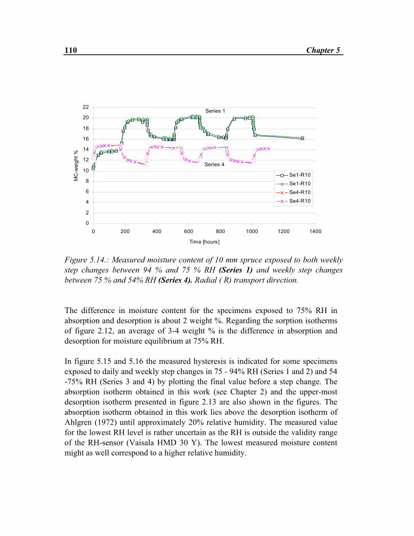
110 Chapter 5
0
2
4
6
8
10
12
14
16
18
20
22
0 200 400 600 800 1000 1200 1400
Time [hours]
MC
-wei
ght %
Se1-R10
Se1-R10
Se4-R10
Se4-R10
Series 4
Series 1
Figure 5.14.: Measured moisture content of 10 mm spruce exposed to both weekly step changes between 94 % and 75 % RH (Series 1) and weekly step changes between 75 % and 54% RH (Series 4). Radial ( R) transport direction. The difference in moisture content for the specimens exposed to 75% RH in absorption and desorption is about 2 weight %. Regarding the sorption isotherms of figure 2.12, an average of 3-4 weight % is the difference in absorption and desorption for moisture equilibrium at 75% RH. In figure 5.15 and 5.16 the measured hysteresis is indicated for some specimens exposed to daily and weekly step changes in 75 - 94% RH (Series 1 and 2) and 54 -75% RH (Series 3 and 4) by plotting the final value before a step change. The absorption isotherm obtained in this work (see Chapter 2) and the upper-most desorption isotherm presented in figure 2.13 are also shown in the figures. The absorption isotherm obtained in this work lies above the desorption isotherm of Ahlgren (1972) until approximately 20% relative humidity. The measured value for the lowest RH level is rather uncertain as the RH is outside the validity range of the RH-sensor (Vaisala HMD 30 Y). The lowest measured moisture content might as well correspond to a higher relative humidity.
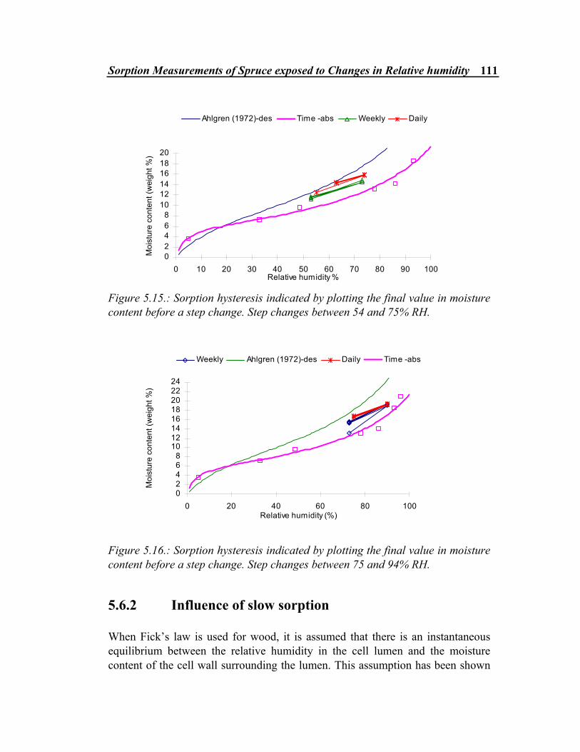
Sorption Measurements of Spruce exposed to Changes in Relative humidity 111
02468
101214161820
0 10 20 30 40 50 60 70 80 90 100Relative humidity %
Moi
stur
e co
nten
t (w
eigh
t %)
Ahlgren (1972)-des Time -abs Weekly Daily
Figure 5.15.: Sorption hysteresis indicated by plotting the final value in moisture content before a step change. Step changes between 54 and 75% RH.
02468
1012141618202224
0 20 40 60 80 100Relative humidity (%)
Moi
stur
e co
nten
t (w
eigh
t %)
Weekly Ahlgren (1972)-des Daily Time -abs
Figure 5.16.: Sorption hysteresis indicated by plotting the final value in moisture content before a step change. Step changes between 75 and 94% RH.
5.6.2 Influence of slow sorption When Fick’s law is used for wood, it is assumed that there is an instantaneous equilibrium between the relative humidity in the cell lumen and the moisture content of the cell wall surrounding the lumen. This assumption has been shown
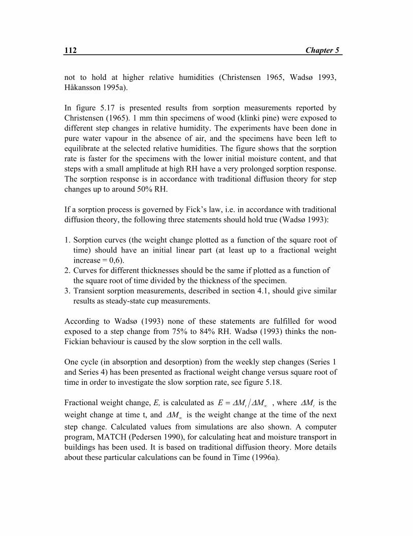
112 Chapter 5
not to hold at higher relative humidities (Christensen 1965, Wadsø 1993, Håkansson 1995a). In figure 5.17 is presented results from sorption measurements reported by Christensen (1965). 1 mm thin specimens of wood (klinki pine) were exposed to different step changes in relative humidity. The experiments have been done in pure water vapour in the absence of air, and the specimens have been left to equilibrate at the selected relative humidities. The figure shows that the sorption rate is faster for the specimens with the lower initial moisture content, and that steps with a small amplitude at high RH have a very prolonged sorption response. The sorption response is in accordance with traditional diffusion theory for step changes up to around 50% RH. If a sorption process is governed by Fick’s law, i.e. in accordance with traditional diffusion theory, the following three statements should hold true (Wadsø 1993): 1. Sorption curves (the weight change plotted as a function of the square root of
time) should have an initial linear part (at least up to a fractional weight increase = 0,6).
2. Curves for different thicknesses should be the same if plotted as a function of the square root of time divided by the thickness of the specimen.
3. Transient sorption measurements, described in section 4.1, should give similar results as steady-state cup measurements.
According to Wadsø (1993) none of these statements are fulfilled for wood exposed to a step change from 75% to 84% RH. Wadsø (1993) thinks the non-Fickian behaviour is caused by the slow sorption in the cell walls. One cycle (in absorption and desorption) from the weekly step changes (Series 1 and Series 4) has been presented as fractional weight change versus square root of time in order to investigate the slow sorption rate, see figure 5.18. Fractional weight change, E, is calculated as E M Mt= ∞∆ ∆ , where ∆Mt is the weight change at time t, and ∆M∞ is the weight change at the time of the next step change. Calculated values from simulations are also shown. A computer program, MATCH (Pedersen 1990), for calculating heat and moisture transport in buildings has been used. It is based on traditional diffusion theory. More details about these particular calculations can be found in Time (1996a).
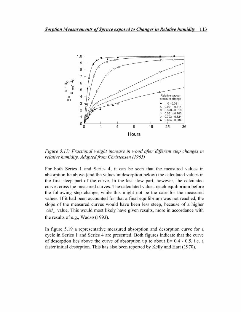
Sorption Measurements of Spruce exposed to Changes in Relative humidity 113
���
�
�
�
�
�
�
�
�� � �� �� ��
� ���
������������ �����������������
������������������������������������������������������������������
�����
�
���������
��
!
Figure 5.17: Fractional weight increase in wood after different step changes in relative humidity. Adapted from Christensen (1965) For both Series 1 and Series 4, it can be seen that the measured values in absorption lie above (and the values in desorption below) the calculated values in the first steep part of the curve. In the last slow part, however, the calculated curves cross the measured curves. The calculated values reach equilibrium before the following step change, while this might not be the case for the measured values. If it had been accounted for that a final equilibrium was not reached, the slope of the measured curves would have been less steep, because of a higher ∆M∞ value. This would most likely have given results, more in accordance with the results of e.g., Wadsø (1993). In figure 5.19 a representative measured absorption and desorption curve for a cycle in Series 1 and Series 4 are presented. Both figures indicate that the curve of desorption lies above the curve of absorption up to about E= 0.4 - 0.5, i.e. a faster initial desorption. This has also been reported by Kelly and Hart (1970).
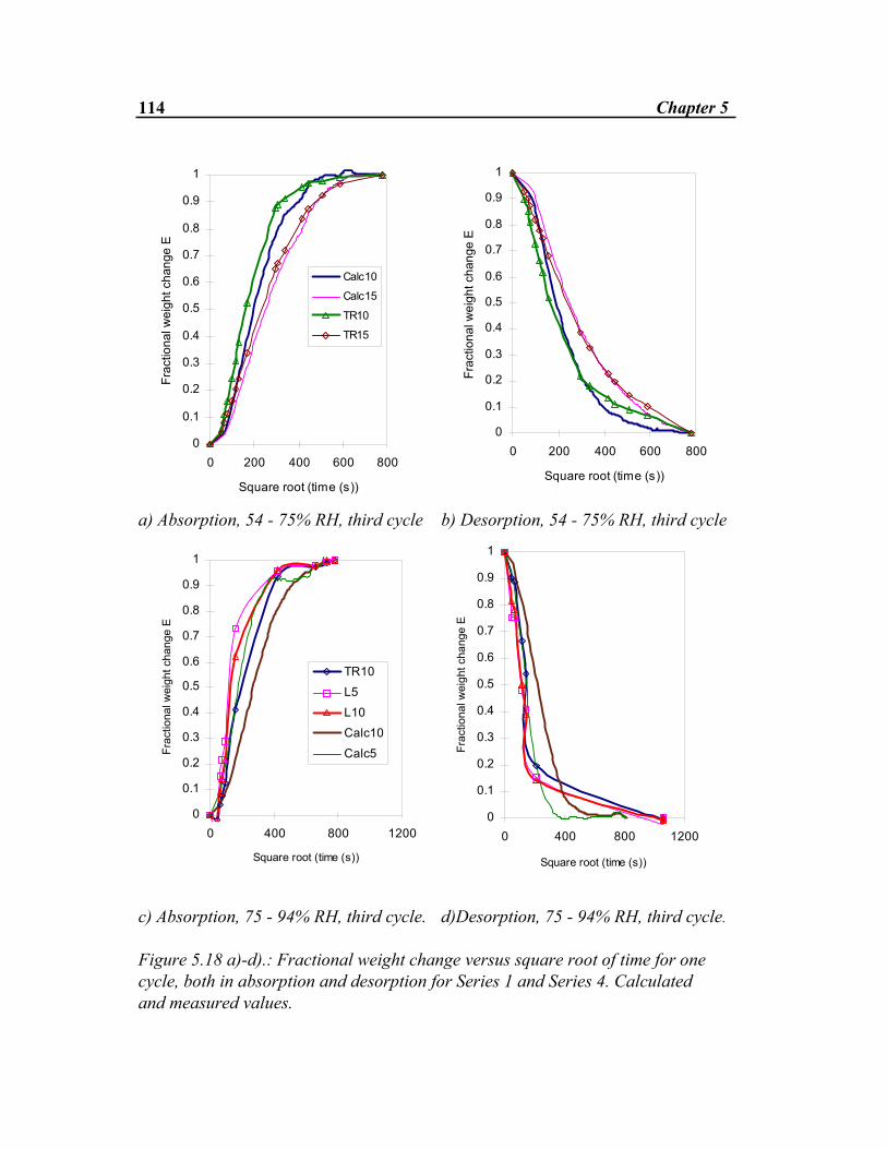
114 Chapter 5
0
0.1
0.2
0.3
0.4
0.5
0.6
0.7
0.8
0.9
1
0 200 400 600 800
Square root (time (s))
Frac
tiona
l wei
ght c
hang
e E
Calc10
Calc15
TR10
TR15
0
0.1
0.2
0.3
0.4
0.5
0.6
0.7
0.8
0.9
1
0 200 400 600 800
Square root (time (s))Fr
actio
nal w
eigh
t cha
nge
E
a) Absorption, 54 - 75% RH, third cycle b) Desorption, 54 - 75% RH, third cycle
0
0.1
0.2
0.3
0.4
0.5
0.6
0.7
0.8
0.9
1
0 400 800 1200
Square root (time (s))
Frac
tiona
l wei
ght c
hang
e E
TR10
L5
L10
Calc10
Calc5
0
0.1
0.2
0.3
0.4
0.5
0.6
0.7
0.8
0.9
1
0 400 800 1200
Square root (time (s))
Frac
tiona
l wei
ght c
hang
e E
c) Absorption, 75 - 94% RH, third cycle. d)Desorption, 75 - 94% RH, third cycle. Figure 5.18 a)-d).: Fractional weight change versus square root of time for one cycle, both in absorption and desorption for Series 1 and Series 4. Calculated and measured values.

Sorption Measurements of Spruce exposed to Changes in Relative humidity 115
0
0.1
0.2
0.3
0.4
0.5
0.6
0.7
0.8
0.9
1
0 200 400 600 800Square root (time (s))
Frac
tiona
l wei
ght c
hang
e E
TR10-AbsTR15-AbsTR10-DesTR15-Des
0
0.1
0.2
0.3
0.4
0.5
0.6
0.7
0.8
0.9
1
0 200 400 600 800Square root (time(s))
Frac
tiona
l wei
ght c
hang
e E
TR10-AbsL5-AbsL10-AbsTR10-DesL5-DesL10-Des
a) Series 4, 54 - 75% RH. Third cycle. b) Series 1, 75 - 94% RH. Second cycle. Figure 5.19 a) - b).:Fractional weight versus square root of time. Weekly step changes in absorption and desorption. Measured values. Three statements that should hold true if a sorption process is governed by Fick’s law have been presented. One of these statements is that curves for different thicknesses should be the same if plotted as a function of the square root of time divided by the thickness of the specimen. Such curves for absorption are presented in figure 5.20. We can see that there is a good conformity for the step change between 54% and 75% RH (figure 5.20 a). This is not the case for the step change between 74% and 94% RH (figure 5.20 b). From figure 5.20 it can be seen that the fractional weight change is rather slow in the very beginning of a cycle. When the vessels are switched, the room air gets in contact with the specimens for about one minute. From the climatic diagrams shown in Appendix 5.A, it can be seen that the RH level in the vessel has a drop during a change. This means that the specimens are exposed to a lower RH for a very short time, and one reason for the initial delay may be the drop in RH during the change of vessel.
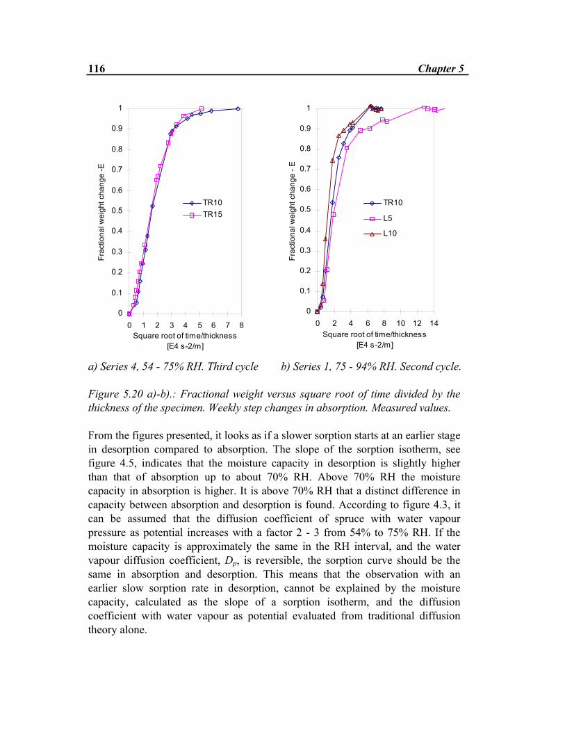
116 Chapter 5
0
0.1
0.2
0.3
0.4
0.5
0.6
0.7
0.8
0.9
1
0 1 2 3 4 5 6 7 8Square root of time/thickness
[E4 s-2/m]
Frac
tiona
l wei
ght c
hang
e -E
TR10TR15
0
0.1
0.2
0.3
0.4
0.5
0.6
0.7
0.8
0.9
1
0 2 4 6 8 10 12 14Square root of time/thickness
[E4 s-2/m]
Frac
tiona
l wei
ght c
hang
e - E
TR10
L5
L10
a) Series 4, 54 - 75% RH. Third cycle b) Series 1, 75 - 94% RH. Second cycle. Figure 5.20 a)-b).: Fractional weight versus square root of time divided by the thickness of the specimen. Weekly step changes in absorption. Measured values. From the figures presented, it looks as if a slower sorption starts at an earlier stage in desorption compared to absorption. The slope of the sorption isotherm, see figure 4.5, indicates that the moisture capacity in desorption is slightly higher than that of absorption up to about 70% RH. Above 70% RH the moisture capacity in absorption is higher. It is above 70% RH that a distinct difference in capacity between absorption and desorption is found. According to figure 4.3, it can be assumed that the diffusion coefficient of spruce with water vapour pressure as potential increases with a factor 2 - 3 from 54% to 75% RH. If the moisture capacity is approximately the same in the RH interval, and the water vapour diffusion coefficient, Dp, is reversible, the sorption curve should be the same in absorption and desorption. This means that the observation with an earlier slow sorption rate in desorption, cannot be explained by the moisture capacity, calculated as the slope of a sorption isotherm, and the diffusion coefficient with water vapour as potential evaluated from traditional diffusion theory alone.
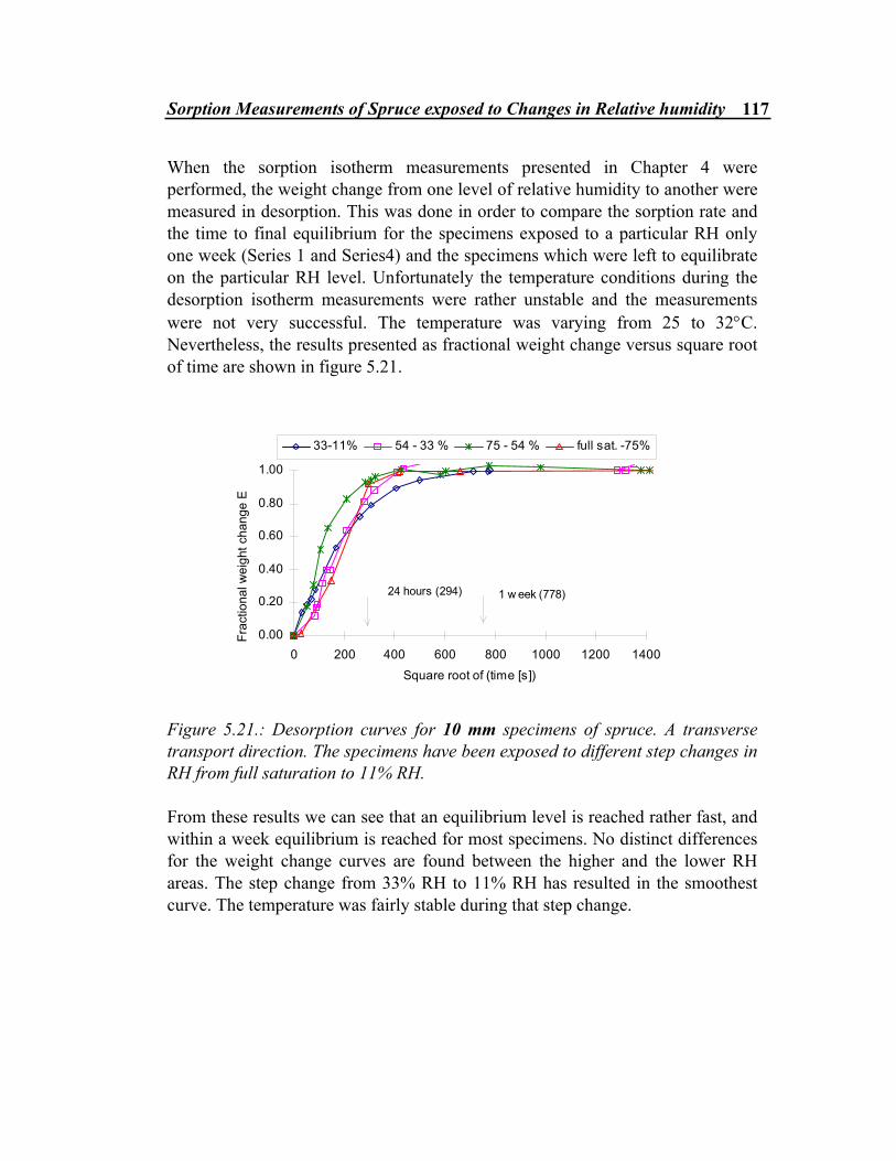
Sorption Measurements of Spruce exposed to Changes in Relative humidity 117
When the sorption isotherm measurements presented in Chapter 4 were performed, the weight change from one level of relative humidity to another were measured in desorption. This was done in order to compare the sorption rate and the time to final equilibrium for the specimens exposed to a particular RH only one week (Series 1 and Series4) and the specimens which were left to equilibrate on the particular RH level. Unfortunately the temperature conditions during the desorption isotherm measurements were rather unstable and the measurements were not very successful. The temperature was varying from 25 to 32°C. Nevertheless, the results presented as fractional weight change versus square root of time are shown in figure 5.21.
0.00
0.20
0.40
0.60
0.80
1.00
0 200 400 600 800 1000 1200 1400Square root of (time [s])
Frac
tiona
l wei
ght c
hang
e E
33-11% 54 - 33 % 75 - 54 % full sat. -75%
24 hours (294) 1 w eek (778)
Figure 5.21.: Desorption curves for 10 mm specimens of spruce. A transverse transport direction. The specimens have been exposed to different step changes in RH from full saturation to 11% RH. From these results we can see that an equilibrium level is reached rather fast, and within a week equilibrium is reached for most specimens. No distinct differences for the weight change curves are found between the higher and the lower RH areas. The step change from 33% RH to 11% RH has resulted in the smoothest curve. The temperature was fairly stable during that step change.
118 Chapter 5
5.7 Conclusions Experimental investigations on wood exposed to cyclic step changes in relative humidity have been done. Results from four different series with daily and weekly cycles between two different levels have been reported. A two-step sorption process has been observed with the major change in moisture content in the first fast initial part. No significant phase lag has been observed for neither transverse nor longitudinal specimens up to 10 mm thickness. A repetitive pattern in moisture content change is found for both weekly and daily changes. The same level of moisture content is reached in both absorption and desorption every cycle. Although the average moisture content has been measured only, the fast response in moisture sorption indicates that significant moisture gradients are present immediately after a relatively large change in surrounding humidity.
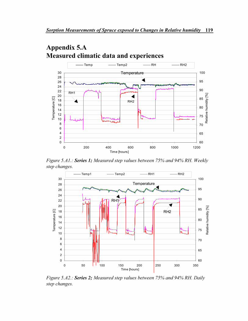
Sorption Measurements of Spruce exposed to Changes in Relative humidity 119
Appendix 5.A
Measured climatic data and experiences
02468
1012141618202224262830
0 200 400 600 800 1000 1200Time [hours]
Tem
pera
ture
[C]
60
65
70
75
80
85
90
95
100
Rel
ativ
e hu
mid
ity [%
]
Temp Temp2 RH RH2
RH1
RH2
Temperature
Figure 5.A1.: Series 1; Measured step values between 75% and 94% RH. Weekly step changes.
0
2
4
6
8
10
12
14
16
18
20
22
24
26
28
30
0 50 100 150 200 250 300 350Time [hours]
Tem
pera
ture
[C]
60
65
70
75
80
85
90
95
100
Rel
ativ
e hu
mid
ity [%
]
Temp1 Temp2 RH1 RH2
Temperature
RH2
RH1
Figure 5.A2.: Series 2; Measured step values between 75% and 94% RH. Daily step changes.

120 Chapter 5
02468
1012141618202224262830
0 50 100 150 200 250 300 350Time [hours]
Tem
pera
ture
[C]
40
45
50
55
60
65
70
75
80
85
90
Rel
ativ
e hu
mid
ity [%
]
Temp1 Temp2 RH1 RH2
Temperature
RH1
RH2
Figure 5.A3.: Series 3; Measured step values between 54% and 75% RH. Daily step changes.
02468
1012141618202224262830
0 200 400 600 800 1000 1200
Time - [hours]
Tem
pera
ture
[C]
40
45
50
55
60
65
70
75
80
85
90
Rel
ativ
e hu
mid
ity %
Temp1 Temp2 RH1 RH2
RH1
RH2
Temperature
Figure 5.A4.: Series 4; Measured step values between 54% and 75% RH. Weekly step changes.
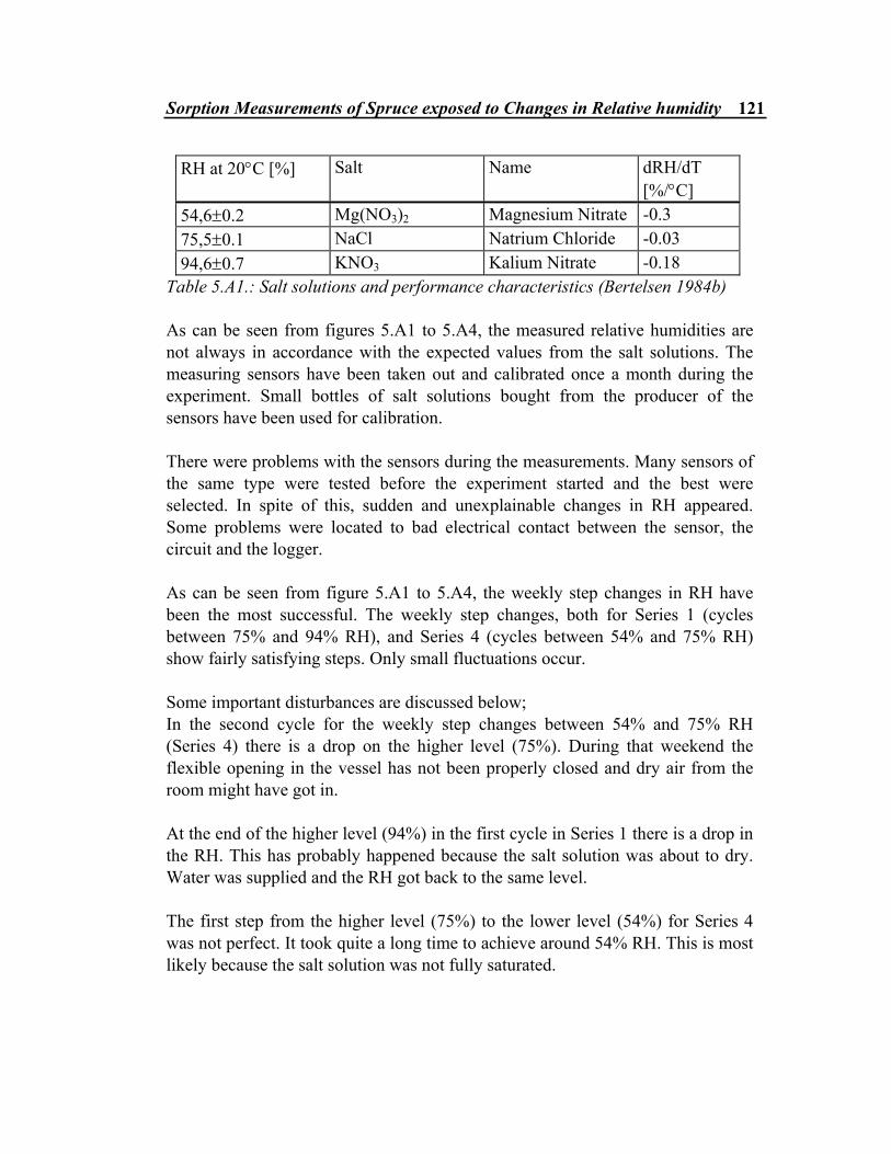
Sorption Measurements of Spruce exposed to Changes in Relative humidity 121
RH at 20°C [%] Salt Name dRH/dT [%/°C]
54,6±0.2 Mg(NO3)2 Magnesium Nitrate -0.3 75,5±0.1 NaCl Natrium Chloride -0.03 94,6±0.7 KNO3 Kalium Nitrate -0.18
Table 5.A1.: Salt solutions and performance characteristics (Bertelsen 1984b) As can be seen from figures 5.A1 to 5.A4, the measured relative humidities are not always in accordance with the expected values from the salt solutions. The measuring sensors have been taken out and calibrated once a month during the experiment. Small bottles of salt solutions bought from the producer of the sensors have been used for calibration. There were problems with the sensors during the measurements. Many sensors of the same type were tested before the experiment started and the best were selected. In spite of this, sudden and unexplainable changes in RH appeared. Some problems were located to bad electrical contact between the sensor, the circuit and the logger. As can be seen from figure 5.A1 to 5.A4, the weekly step changes in RH have been the most successful. The weekly step changes, both for Series 1 (cycles between 75% and 94% RH), and Series 4 (cycles between 54% and 75% RH) show fairly satisfying steps. Only small fluctuations occur. Some important disturbances are discussed below; In the second cycle for the weekly step changes between 54% and 75% RH (Series 4) there is a drop on the higher level (75%). During that weekend the flexible opening in the vessel has not been properly closed and dry air from the room might have got in. At the end of the higher level (94%) in the first cycle in Series 1 there is a drop in the RH. This has probably happened because the salt solution was about to dry. Water was supplied and the RH got back to the same level. The first step from the higher level (75%) to the lower level (54%) for Series 4 was not perfect. It took quite a long time to achieve around 54% RH. This is most likely because the salt solution was not fully saturated.
122 Chapter 5
The daily step changes are not that satisfying, especially not for the step changes between 75% and 94% RH (Series 2). Measuring data for the first 2 days have been lost and for the following three days one of the RH-sensors showed very unstable values. This was most likely due to bad electrical contact between the sensor and the logger. A circuit was changed after 3 days, and the RH values stabilised. For both Series 2 and 3, daily cycles, a slight increase in RH is seen on the upper RH-level just before the step change. This is unexpected and no explanation has been found. For Series 3, the lower RH-level was difficult to achieve. The given recipe (Bertelsen 1984b) on how to achieve a saturated salt solution from Mg(NO3)2 was not found correct. Much more salt than expected were needed to obtain around 54% RH. For some of the step changes a drop in RH when changing the vessels are seen. Depending on the time to logging, after the vessels have changed, this lower RH (room RH) can be seen on the curve. The rise in RH after a change is rather fast. Measurements showed that it took about 10 minutes to reach 90% of a step change from 35% (room RH) to 75%. The fan has been switched off at different occasions. The longest period was 12 hours (one night). This has, as far as the weight results have shown, not affected the measurements. Mould growth has not been observed on any specimens at any time. Some of the thinnest specimens failed during the experiment. These specimens curved and the polyethylene tape came off.

Chapter 6
Modelling of Transient Moisture Transport and Hysteresis in Wood In this chapter, a transient model for moisture transport in wood is set up. The model is based on Fick’s law with water vapour pressure and temperature as driving potentials. A model for hysteresis has been proposed and included in the model. Comparisons between experimental results presented in Chapter 5 and calculations have been performed. The model only deals with moisture transport in the hygroscopic region, liquid water is not included. Theoretical approaches and experiences with modelling of moisture transport in wood are thoroughly discussed in Chapter 3, and will not be discussed any further in this chapter.
6.1 Introduction Discrepancies between measurements and calculations for moisture conditions in wood in building structures have made a more thorough study on moisture transport processes in wood necessary. In this chapter, a model for transient
124 Chapter 6
moisture transport in wood is set up in order to investigate the influence of material properties and hysteresis on moisture sorption. Calculations are compared with the experimental results presented in Chapter 5. For moisture transport calculations in the hygroscopic region, a Fickian approach , i.e. moisture transport by diffusion, is normally used. The selected driving potential often differs and because of this the transport coefficients (diffusion coefficients) themselves differ. A few models are commercial available for heat, air and moisture transport calculations in building envelopes, but many more exist only as research tools. Among all models reported in Hens (1996), only two out of 37 reported codes explicitly mention the effect of hysteresis. Only one of the two mentioned models is, as far as I know, a commercial available computer program. This is the computer program named MATCH (Pedersen 1990). The author has used the computer program MATCH in previously reported work (Time 1996a,b). For the purpose of research the applicability of commercial available computer programs is often limited. From a building engineering or a building science point of view, a driving potential which is continuous across a construction, no matter type of material, is to be preferred. Moisture content or water vapour pressure in the air is such a potential. Temperature and relative humidity can be measured within building envelopes, and from that it is fairly easy to evaluate vapour pressure and saturation vapour pressure. It has been reported in the past that moisture transport in wood is not always obeying Fick’s law (Christensen 1965, Wadsø 1993). This has especially been seen when wood samples have been equilibrated after having been exposed to a relatively small step change in relative humidity at higher relative humidity levels. Wood in buildings, however, is very rarely exposed to steady-state conditions. It goes through diurnal and annual moisture cycles, and smaller or larger changes in surrounding temperature and/or relative humidity happen all the time. From the results presented in Chapter 5 it can be seen that even fairly small changes in relative humidity give changes in the average moisture content of wooden specimens. Former research and investigations conducted in this work have shown that there are fairly large variations in material properties for wood in general and spruce in particular. This means that significant variations exist for material parameters included in numerical models for moisture transport in wood. Over the years it has been reported that diffusion coefficients obtained by steady-state cup methods
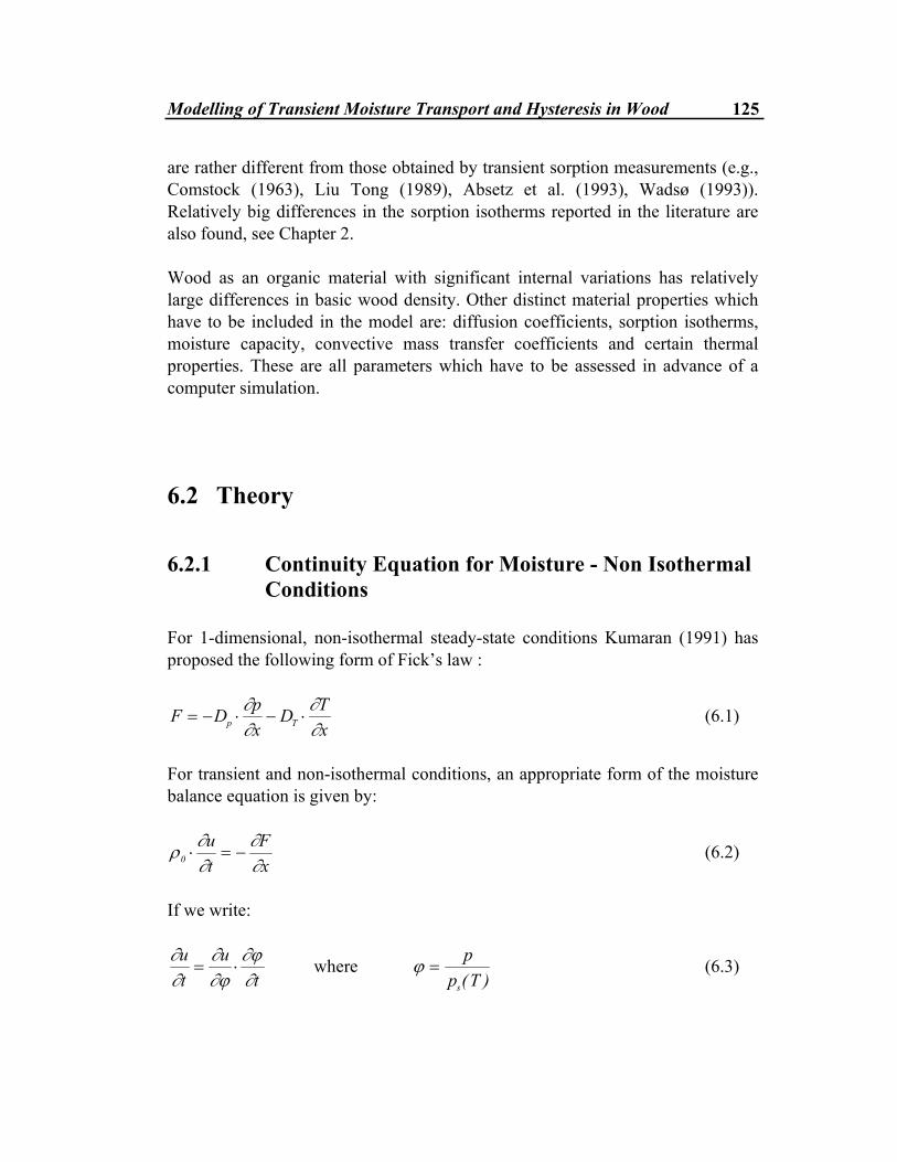
Modelling of Transient Moisture Transport and Hysteresis in Wood 125
are rather different from those obtained by transient sorption measurements (e.g., Comstock (1963), Liu Tong (1989), Absetz et al. (1993), Wadsø (1993)). Relatively big differences in the sorption isotherms reported in the literature are also found, see Chapter 2. Wood as an organic material with significant internal variations has relatively large differences in basic wood density. Other distinct material properties which have to be included in the model are: diffusion coefficients, sorption isotherms, moisture capacity, convective mass transfer coefficients and certain thermal properties. These are all parameters which have to be assessed in advance of a computer simulation.
6.2 Theory
6.2.1 Continuity Equation for Moisture - Non Isothermal Conditions For 1-dimensional, non-isothermal steady-state conditions Kumaran (1991) has proposed the following form of Fick’s law :
F D px
D Txp T= − ⋅ − ⋅
∂∂
∂∂
(6.1)
For transient and non-isothermal conditions, an appropriate form of the moisture balance equation is given by:
ρ ∂∂
∂∂0 ⋅ = −
ut
Fx
(6.2)
If we write: ∂∂
∂∂ϕ
∂ϕ∂
ut
ut
= ⋅ where ϕ =p
p Ts( ) (6.3)

126 Chapter 6
and then combine (6.1) and (6.2), we get: ρ ∂∂ϕ
∂ϕ∂
∂∂
∂∂
∂∂0 ⋅ ⋅ = − − ⋅ − ⋅
ut x
D px
D Txp T
Substituting p into ϕ we get
ρ ∂∂ϕ
∂
∂∂∂
∂∂
∂∂0 ⋅ ⋅ = − − ⋅ − ⋅
uppt x
D px
D Tx
sp T
( )
and further
∂
∂
∂∂
∂∂
( )ppt
pt
p p pt
ps
ss
s
=⋅ − ⋅
2 (6.4)
This gives us the following equation
ρ ∂∂ϕ
∂∂
∂∂ ∂
∂∂∂
∂∂0 2⋅ ⋅
⋅ − ⋅
= − − ⋅ − ⋅
upt
p p pt
p xD p
xD T
x
ss
sp T (6.5)
∂∂ϕ
u is a non-linear expression for the moisture capacity which is solved
separately before the main equation (6.5). Dp is the water vapour diffusion coefficient with vapour pressure as a potential, also being a non -linear function of water vapour pressure (or moisture content u or relative humidity RH) and temperature. It also has to be solved separately before the main equation. DT is the thermal moisture diffusion coefficient, a quantity which can be a complex function of both u and T (Kumaran 1991). Hardly any values for this property are known apart from earlier Russian work as reported by Luikov (1966) for instance. Earlier work on moisture diffusion have tended to concentrate on a single-variable driving potential for moisture transfer (e.g., water vapour pressure gradient or moisture concentration gradient). Under isothermal conditions these two can be related through the sorption isotherm of

Modelling of Transient Moisture Transport and Hysteresis in Wood 127
the material. Under non-isothermal conditions, however, the diffusive driving potential is not well understood (Cunningham 1992). Because the equations for these variables are solved separately before the main equation, and can be looked upon as constants for a time-step, equation (6.5) can be expressed as
ρ ∂∂ϕ
∂∂
∂∂ ∂
∂∂∂0 2
2
2
2
2⋅ ⋅⋅ − ⋅
= ⋅ + ⋅
upt
p p pt
pD p
xD T
x
ss
sp T (6.6)
The above equation is solved for p. ∂∂pts and ∂
∂
2
2
Tx
are solved before the main equation (6.6) so that T and ps can be
looked upon as constants when solving (6.6). The transient heat flow equation has the following one-dimensional form ∂∂
∂∂
Tt
aT
x= ⋅
2
2 , a
c=
⋅λρ0
(6.7)
The following equation has been used to calculate the water vapour saturation pressure (Danvak 1987)
pTs = −−
exp . ..
23 5771 4042 937 58
(Pa) (6.8)
For the boundaries, the following equations for temperature and vapour pressure have been solved
ρ λ0
1
12⋅ ⋅ ⋅
−= − + −
+
+ ∞c x T Tt x
T T h T Tit
it
it
it
it∆
∆ ∆( ) ( ) (6.9)
∆
∆ ∆x A u
tD
xA p p D
xA T T h A p pp
it
it T
it
it
p it
2 0 1 1⋅ ⋅ ⋅ = ⋅ ⋅ − + ⋅ ⋅ − + ⋅ ⋅ −+ + ∞ρ ∂∂
( ) ( ) ( ) (6.10)

128 Chapter 6
The dry wood density (ρ0) is a constant given as an initial value, so are also the convective heat- transfer coefficient (h), the convective mass-transfer coefficient1 (hp), the thermal conductivity (λ), heat capacity (c) and the thermal diffusivity (a). The thermal moisture-diffusion coefficient is assumed to be a constant independent of relative humidity, but limited data suggest that this might not be the case (Luikov 1966).
6.3 Numerical solution method An explicit finite-difference method has been used (forward difference method). Hourly boundary values (air temperature and relative humidity) are read from file. The moisture content, moisture capacity, diffusion coefficient, temperature- , saturation vapour pressure- and vapour pressure fields are being updated at each time-step. If hysteresis is included, the moisture content situation is checked every time-step in order to decide which sorption isotherm or intermediate curve to join. An hourly value of the average moisture content for all control volumes is recorded to file. See figure 6.1.
6.4 Modelling of material properties
6.4.1 Diffusion coefficients In Chapter 4 it has been shown that the diffusion coefficient, Dp, is dependent of the relative humidity. Three different approaches for calculating the diffusion coefficient have been used in this work, see figure 6.2. All values have been selected on the basis of the measured values presented in figure 4.3. The first approach employs a constant diffusion coefficient equal to 6.0⋅10-12 kg⋅m-1s-1 Pa-1 for the transport in the transverse direction and 60.0⋅10-12 kg⋅m-1s-1 Pa-1
for the transport in the longitudinal direction.
1 The convective mass-transfer coefficient is also often called the surface mass-transfer coefficient
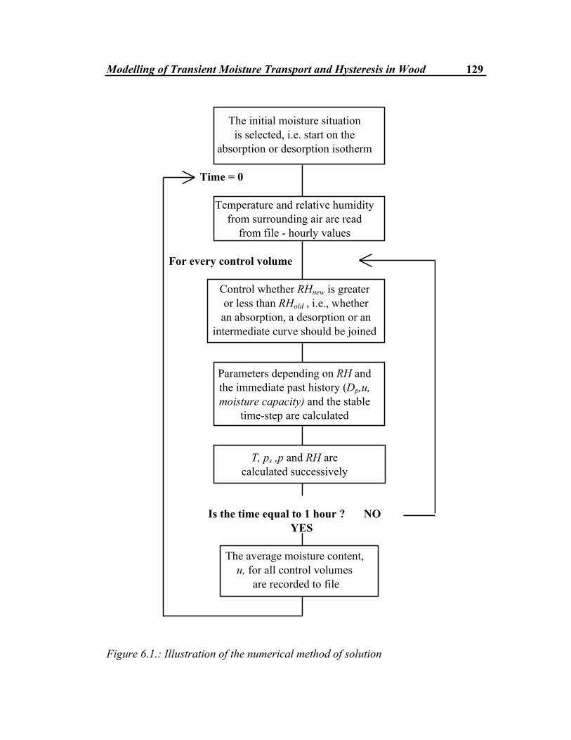
Modelling of Transient Moisture Transport and Hysteresis in Wood 129
The initial moisture situation
is selected, i.e. start on the absorption or desorption isotherm
Time = 0
Temperature and relative humidity from surrounding air are read
from file - hourly values For every control volume
Control whether RHnew is greater or less than RHold , i.e., whether an absorption, a desorption or an
intermediate curve should be joined
Parameters depending on RH and the immediate past history (Dp,u, moisture capacity) and the stable
time-step are calculated
T, ps ,p and RH are calculated successively
Is the time equal to 1 hour ? NO YES
The average moisture content,
u, for all control volumes are recorded to file
Figure 6.1.: Illustration of the numerical method of solution
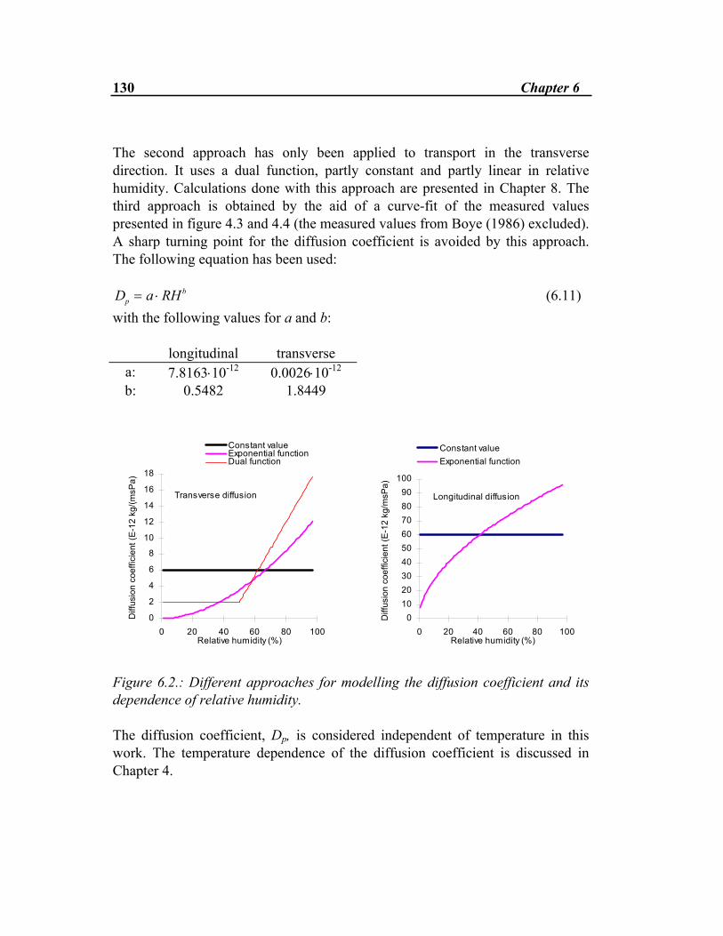
130 Chapter 6
The second approach has only been applied to transport in the transverse direction. It uses a dual function, partly constant and partly linear in relative humidity. Calculations done with this approach are presented in Chapter 8. The third approach is obtained by the aid of a curve-fit of the measured values presented in figure 4.3 and 4.4 (the measured values from Boye (1986) excluded). A sharp turning point for the diffusion coefficient is avoided by this approach. The following equation has been used: D a RHp
b= ⋅ (6.11) with the following values for a and b:
longitudinal transverse
a: 7.8163⋅10-12 0.0026⋅10-12 b: 0.5482 1.8449
0
2
4
6
8
10
12
14
16
18
0 20 40 60 80 100Relative humidity (%)
Diff
usio
n co
effic
ient
(E-1
2 kg
/(msP
a)
Constant valueExponential functionDual function
Transverse diffusion
0102030405060708090
100
0 20 40 60 80 100Relative humidity (%)
Diff
usio
n co
effic
ient
(E-1
2 kg
/msP
a)
Constant valueExponential function
Longitudinal diffusion
Figure 6.2.: Different approaches for modelling the diffusion coefficient and its dependence of relative humidity. The diffusion coefficient, Dp, is considered independent of temperature in this work. The temperature dependence of the diffusion coefficient is discussed in Chapter 4.
Modelling of Transient Moisture Transport and Hysteresis in Wood 131
The thermal moisture diffusion coefficient, DT , has been set equal to zero for the calculations in this chapter. As there are very small temperature gradients in time and none in space, there will be no influences of the thermal moisture diffusion.
6.4.2 Moisture capacity and moisture content The Hailwood and Horrobin equation, which has been found suitable for wood (Skaar 1988, Liu Tong 1989, Absetz et al. 1993) has been used for calculating the equilibrium moisture content as a function of relative humidity. This topic is thoroughly discussed in Chapter 2. The equation is
u RHA B RH C RH
=+ ⋅ − ⋅ 2
(6.12)
were A,B and C are curve fitting parameters. The derivative of the Hailwood and Horrobin equation, which represents the slope of the sorption isotherm and thus the moisture capacity, is expressed with the same curve-fitting parameters A, B, C as follows: ∂∂
uRH
A C RHA A B RH B A C RH B C RH C RH
=+ ⋅
+ ⋅ ⋅ ⋅ + − ⋅ ⋅ ⋅ − ⋅ ⋅ ⋅ + ⋅
2
2 2 2 3 2 42 2 2( )
(6.13) Equations obtained by different researchers, see table 2.2, figure 2.13 and 4.5, have been used in the calculations. If hysteresis is included both moisture content and moisture capacity are evaluated differently. This is discussed in section 6.5. Differences in the sorption isotherms for different temperatures have not been included in the modelling work. Sorption isotherms and temperature dependence are discussed in section 2.6 and 2.7.
6.4.3 Convective mass-transfer coefficient The values for the convective mass transfer coefficient are evaluated from the values presented in Wadsø (1993). He has made a thorough literature review and calculated convective mass-transfer coefficients for different surfaces, not only

132 Chapter 6
wood. He has converted all values to hp (the coefficient based on partial vapour pressure differences). Most of the evaluated values for wood are in the order of 1⋅10-9 to 30⋅10-9 kg⋅m-2s-1 Pa-1 with air velocity variations from nearly 0 to about 3 m⋅s-1. In addition to the air velocity, the convective mass-transfer coefficient is also dependent on the length and the geometry of the evaporative surface and the direction of the flow. More details about this can be found in e.g. Wadsø (1993). Two different values for the convective mass transfer coefficient have been used, namely 30⋅10-9 kg⋅m-2s-1 Pa-1 which is often found for wood, and 100⋅10-9 kg⋅m-2s-1 Pa-1, which is a fairly high value for sorption experiments with an air velocity of 0.1 to 0.3 m⋅s-1 and a length of the specimen like 0.07 m.
6.5 Hysteresis
6.5.1 Approaches to modelling Among all codes modelling heat, air and moisture transport in building constructions reported in Hens (1996), only 2 out of 37 reported codes consider the hysteresis effect between absorption and desorption. In MATCH (Pedersen 1990) hysteresis is included. Pedersen models the hysteresis in an empirical way. Empirical formulas are used to describe the moisture capacities on the intermediate curves between moistening and drying. Depending on the current direction of the moisture history, the intermediate curves are asymptotically moving towards the curves describing either the pure desorption or the pure absorption situation. Peralta (1995b) has used the “independent-domain theory” to model hysteresis. From experimental sorption boundary curves and a family of primary desorption intermediate curves reported in (Peralta 1995a), a grid of values is generated. The grid is then used to mathematically obtain several primary desorption scanning curves and secondary and tertiary scanning curves. The model has, as far as I know, not been used in any moisture transport calculations.
Modelling of Transient Moisture Transport and Hysteresis in Wood 133
Håkansson (1995b) has included hysteresis in his model for transient moisture transport in wood. “An envelope” is created by the initial absorption curve and a desorption line from the maximum reached RH-level. Within this “envelope” there are linear intermediate curves. The best fit to experimental moisture sorption data is found when hysteresis is included in several internal levels in his network model. See Håkansson (1995b) for a more detailed description of his model.
6.5.2 Background for the choice of a hysteresis model Very little experimental data exist for intermediate (or scanning) curves for wood. Figure 2.10 shows the intermediate curves presented in Ahlgren (1972) and Peralta (1995a) for spruce and yellow poplar respectively. Chomcharn and Skaar (1983) have performed experimental investigations on three different species from hardwood exposed to sinusoidally varying relative humidity. The relative humidity has been varying between 48 and 78%. Four different cycling periods have been used. The mean value of the moisture capacity for the different species, du/dϕ, has been evaluated over the humidity range covered in their study. They use the expression dynamic moisture capacity. The static moisture capacity on the other hand, is the moisture capacity obtained from the border sorption isotherms. Only small differences in the dynamic moisture capacity are found for the four different cycling periods and only a mean value for each species has been reported. The values for yellow birch, basswood and black cherry are 0.127, 0.121 and 0.150 respectively. The corresponding static values have been evaluated from sorption isotherm data reported in the literature, and they are found to be 0.343, 0.298 and 0.331. From the reported data it is evident that the effective mean slope of an intermediate curve is only about 0.4 as great as that of a static (border) isotherm. A more thorough investigation of the intermediate curves reported in Ahlgren (1972) and Peralta (1995a) has been done. Peralta has reported 4 intermediate curves in desorption with different starting points on the absorption isotherm. The set of specimens were exposed to successively reduced relative humidity stages of about 10% decrement down to 11% RH. Ahlgren (1972) has reported one intermediate curve in absorption which originates from 44% RH on the desorption isotherm, and reaches the border absorption isotherm at 94%. See also figure 2.10.
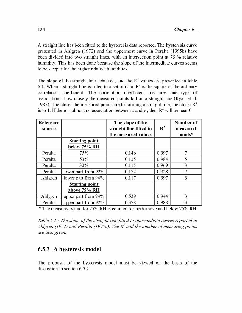
134 Chapter 6
A straight line has been fitted to the hysteresis data reported. The hysteresis curve presented in Ahlgren (1972) and the uppermost curve in Peralta (1995b) have been divided into two straight lines, with an intersection point at 75 % relative humidity. This has been done because the slope of the intermediate curves seems to be steeper for the higher relative humidities. The slope of the straight line achieved, and the R2 values are presented in table 6.1. When a straight line is fitted to a set of data, R2 is the square of the ordinary correlation coefficient. The correlation coefficient measures one type of association - how closely the measured points fall on a straight line (Ryan et al. 1985). The closer the measured points are to forming a straight line, the closer R2 is to 1. If there is almost no association between x and y , then R2 will be near 0. Reference
source The slope of the
straight line fitted to the measured values
R2
Number of measured
points* Starting point
below 75% RH
Peralta 75% 0,146 0,997 7 Peralta 53% 0,125 0,984 5 Peralta 32% 0,115 0,969 3 Peralta lower part-from 92% 0,172 0,928 7
Ahlgren lower part from 94% 0,117 0,997 3 Starting point
above 75% RH
Ahlgren upper part from 94% 0,539 0,944 3 Peralta upper part-from 92% 0,378 0,988 3
* The measured value for 75% RH is counted for both above and below 75% RH Table 6.1.: The slope of the straight line fitted to intermediate curves reported in Ahlgren (1972) and Peralta (1995a). The R2 and the number of measuring points are also given.
6.5.3 A hysteresis model The proposal of the hysteresis model must be viewed on the basis of the discussion in section 6.5.2.
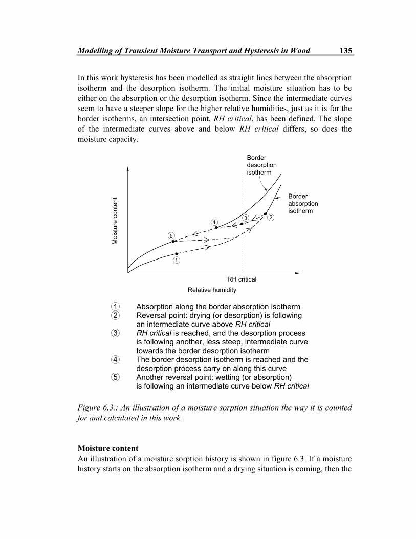
Modelling of Transient Moisture Transport and Hysteresis in Wood 135
In this work hysteresis has been modelled as straight lines between the absorption isotherm and the desorption isotherm. The initial moisture situation has to be either on the absorption or the desorption isotherm. Since the intermediate curves seem to have a steeper slope for the higher relative humidities, just as it is for the border isotherms, an intersection point, RH critical, has been defined. The slope of the intermediate curves above and below RH critical differs, so does the moisture capacity.
�
���
�
���
��
����
�
���� �� ��������� ��
����������
� ���� ��������
���� ������������ ��
�� ���������������� ����� �������������� ���� � � ����������������� ���� ������!���"����#���� ����� �� ��� ����� ����� ������������� �������������� ��� �$������ �� ����������� � ��"����#�������� �$�� � �$��� �� ��� ����� � �#����� ����� ��� ���������� ���� %� ����� ��� ���������� ������ ��� ������� � � ����������� ����������������������� �� ���� ��� � ����������# ���� �����������!� ��"����#��������� �� ��� ����� �� ��#�����������
Figure 6.3.: An illustration of a moisture sorption situation the way it is counted for and calculated in this work. Moisture content An illustration of a moisture sorption history is shown in figure 6.3. If a moisture history starts on the absorption isotherm and a drying situation is coming, then the
136 Chapter 6
moisture content will be calculated according to a change in relative humidity multiplied by the particular slope of the intermediate curve and added to the old moisture content. The procedure will carry on until the desorption isotherm is reached, unless one gets a return, and another absorption situation is coming. If an absorption situation is coming, the same straight line will be followed towards the border absorption isotherm. This means that the slope of the absorption intermediate curve is assumed to be the same as the slope of the desorption intermediate curve. If a cycling absorption and desorption situation occurs, and the border absorption and desorption isotherms are never reached, the moisture content will be calculated according to the same intermediate curve(s). Moisture capacity The moisture capacity for the hysteresis situation is set either • as different constants for the relative humidities below and above RH critical,
or as • a constant value below RH critical and a linear function of RH above RH
critical The last approach is not in accordance with the fact that the moisture capacity is equal to the slope of the sorption isotherm. However, both approaches have been used in order to compare them.
6.6 Comparison of calculations and experimental results A selection of numerical calculations has been done in order to compare the model, with hysteresis included, with the experimental results given in Chapter 5.
6.6.1 Influence of input parameters in general The value of different input parameters has been varied. It has been experienced, that the most important parameter, in order to obtain a good agreement between calculations and measurements, is the level of the absorption and the desorption isotherm, and the slope of the intermediate curves.
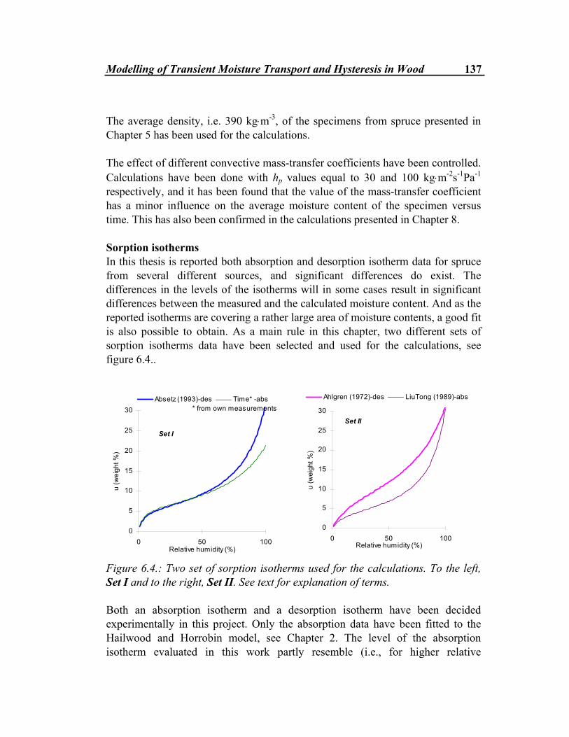
Modelling of Transient Moisture Transport and Hysteresis in Wood 137
The average density, i.e. 390 kg⋅m-3, of the specimens from spruce presented in Chapter 5 has been used for the calculations. The effect of different convective mass-transfer coefficients have been controlled. Calculations have been done with hp values equal to 30 and 100 kg⋅m-2s-1Pa-1 respectively, and it has been found that the value of the mass-transfer coefficient has a minor influence on the average moisture content of the specimen versus time. This has also been confirmed in the calculations presented in Chapter 8. Sorption isotherms In this thesis is reported both absorption and desorption isotherm data for spruce from several different sources, and significant differences do exist. The differences in the levels of the isotherms will in some cases result in significant differences between the measured and the calculated moisture content. And as the reported isotherms are covering a rather large area of moisture contents, a good fit is also possible to obtain. As a main rule in this chapter, two different sets of sorption isotherms data have been selected and used for the calculations, see figure 6.4..
0
5
10
15
20
25
30
0 50 100Relative humidity (%)
u (w
eigh
t %)
Absetz (1993)-des Time* -abs* from own measurements
Set I
0
5
10
15
20
25
30
0 50 100Relative humidity (%)
u (w
eigh
t %)
Ahlgren (1972)-des LiuTong (1989)-abs
Set II
Figure 6.4.: Two set of sorption isotherms used for the calculations. To the left, Set I and to the right, Set II. See text for explanation of terms. Both an absorption isotherm and a desorption isotherm have been decided experimentally in this project. Only the absorption data have been fitted to the Hailwood and Horrobin model, see Chapter 2. The level of the absorption isotherm evaluated in this work partly resemble (i.e., for higher relative
138 Chapter 6
humidities) the absorption isotherm obtained by Absetz et al. (1993), and also some of the desorption values are on the same level as those obtained by Absetz et al. Because of this, one set of sorption isotherm data, Set I, consists of: the absorption isotherm evaluated in this project, and the desorption isotherm given in Absetz et al. (1993). See figure 6.4. The other set of isotherm data, Set II, has been chosen as the extreme isotherms among the reported isotherms in figure 2.12 and 2.13, i.e., the absorption isotherm of Liu Tong (1989) and the desorption isotherm of Ahlgren (1972). Diffusion coefficients For the calculations presented, the diffusion coefficient has been chosen to be either a constant or an exponential function of the relative humidity, see section 6.4.1. For the calculated moisture content for both weekly and daily cycles, no significant differences have been found between the calculated cases with a constant diffusion coefficient and those with an exponential diffusion coefficient. This is the case for both the longitudinal and the transverse transport direction. Therefore only calculated cases with an exponential diffusion coefficient are shown in the figures 6.5 to 6.10. Slope of the intermediate/hysteresis curve A linear curve fit has been made for the upper part (i.e., from relative humidity around 50 % ) of the sorption isotherms presented in figure 2.12. The major part of these have an average slope between 0.32 and 0.42 with an average of 0.35. This is less than the slope of the intermediate curves above 75 % relative humidity presented in table 6.1. However, these curves are valid above 75 % relative humidity and a steeper slope is to be expected. For modelling of the experimental results presented in Chapter 5, the slopes of the intermediate curves above RH critical equal to those presented in table 6.1 have been found too steep. If too steep slopes are used, the intermediate curve will hardly not be joined. If a moisture desorption situation starts on the absorption isotherm for example, the absorption isotherm will be joined in drying instead of an intermediate curve. This is because the slope of the absorption isotherm is less steep than that of the intermediate curve. A slope of 0.2 for the intermediate curve above RH critical and a slope of 0.1 below have been found more correct in order of magnitude according to the measured results presented in Chapter 5. On the basis of the result presented in Chomcharn and Skaar (1983) and what have been mentioned earlier in this chapter, 0.2 is the 40 % slope of a border isotherm slope of 0.5.
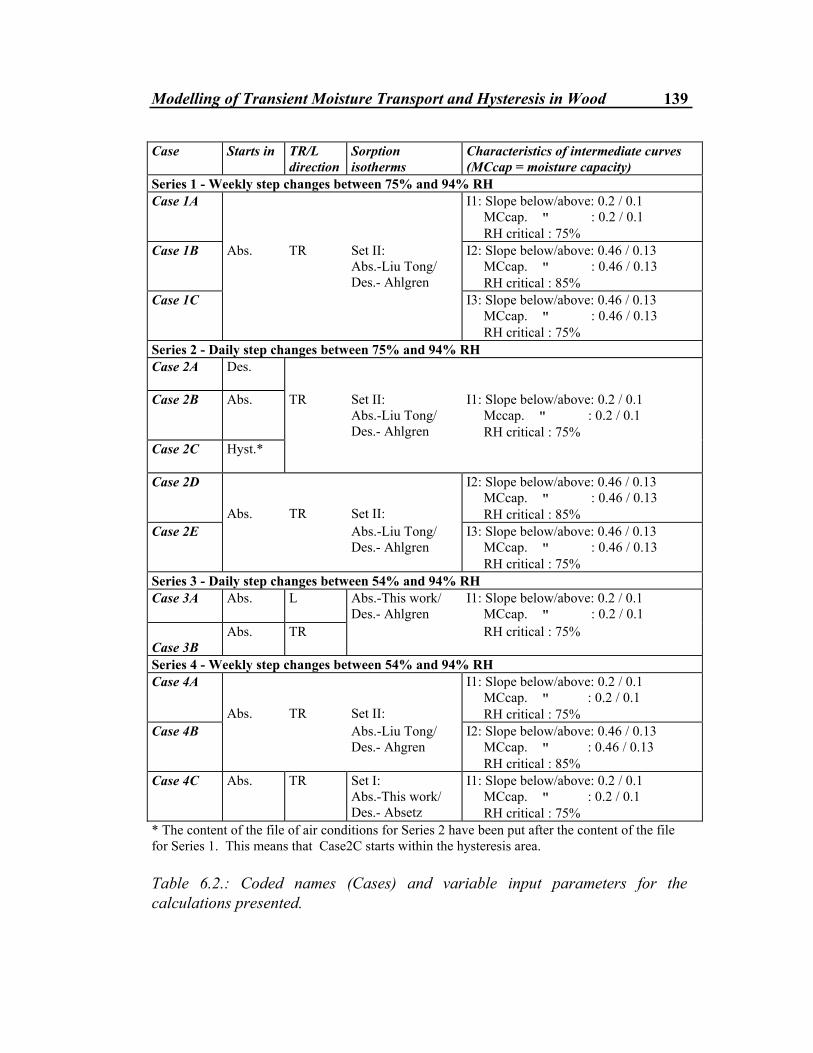
Modelling of Transient Moisture Transport and Hysteresis in Wood 139
Case Starts in TR/L direction
Sorption isotherms
Characteristics of intermediate curves (MCcap = moisture capacity)
Series 1 - Weekly step changes between 75% and 94% RH Case 1A I1: Slope below/above: 0.2 / 0.1
MCcap. " : 0.2 / 0.1 RH critical : 75%
Case 1B Abs. TR Set II: Abs.-Liu Tong/ Des.- Ahlgren
I2: Slope below/above: 0.46 / 0.13 MCcap. " : 0.46 / 0.13 RH critical : 85%
Case 1C I3: Slope below/above: 0.46 / 0.13 MCcap. " : 0.46 / 0.13 RH critical : 75%
Series 2 - Daily step changes between 75% and 94% RH Case 2A
Des.
Case 2B Abs. TR Set II: Abs.-Liu Tong/ Des.- Ahlgren
I1: Slope below/above: 0.2 / 0.1 Mccap. " : 0.2 / 0.1 RH critical : 75%
Case 2C
Hyst.*
Case 2D Abs.
TR
Set II:
I2: Slope below/above: 0.46 / 0.13 MCcap. " : 0.46 / 0.13 RH critical : 85%
Case 2E Abs.-Liu Tong/ Des.- Ahlgren
I3: Slope below/above: 0.46 / 0.13 MCcap. " : 0.46 / 0.13 RH critical : 75%
Series 3 - Daily step changes between 54% and 94% RH Case 3A Abs. L Abs.-This work/
Des.- Ahlgren I1: Slope below/above: 0.2 / 0.1 MCcap. " : 0.2 / 0.1
Case 3B
Abs. TR RH critical : 75%
Series 4 - Weekly step changes between 54% and 94% RH Case 4A
Abs.
TR
Set II:
I1: Slope below/above: 0.2 / 0.1 MCcap. " : 0.2 / 0.1 RH critical : 75%
Case 4B Abs.-Liu Tong/ Des.- Ahgren
I2: Slope below/above: 0.46 / 0.13 MCcap. " : 0.46 / 0.13 RH critical : 85%
Case 4C Abs. TR Set I: Abs.-This work/ Des.- Absetz
I1: Slope below/above: 0.2 / 0.1 MCcap. " : 0.2 / 0.1 RH critical : 75%
* The content of the file of air conditions for Series 2 have been put after the content of the file for Series 1. This means that Case2C starts within the hysteresis area. Table 6.2.: Coded names (Cases) and variable input parameters for the calculations presented.
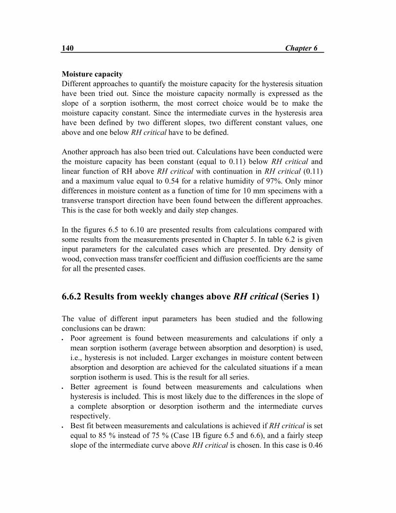
140 Chapter 6
Moisture capacity Different approaches to quantify the moisture capacity for the hysteresis situation have been tried out. Since the moisture capacity normally is expressed as the slope of a sorption isotherm, the most correct choice would be to make the moisture capacity constant. Since the intermediate curves in the hysteresis area have been defined by two different slopes, two different constant values, one above and one below RH critical have to be defined. Another approach has also been tried out. Calculations have been conducted were the moisture capacity has been constant (equal to 0.11) below RH critical and linear function of RH above RH critical with continuation in RH critical (0.11) and a maximum value equal to 0.54 for a relative humidity of 97%. Only minor differences in moisture content as a function of time for 10 mm specimens with a transverse transport direction have been found between the different approaches. This is the case for both weekly and daily step changes. In the figures 6.5 to 6.10 are presented results from calculations compared with some results from the measurements presented in Chapter 5. In table 6.2 is given input parameters for the calculated cases which are presented. Dry density of wood, convection mass transfer coefficient and diffusion coefficients are the same for all the presented cases.
6.6.2 Results from weekly changes above RH critical (Series 1) The value of different input parameters has been studied and the following conclusions can be drawn: • Poor agreement is found between measurements and calculations if only a
mean sorption isotherm (average between absorption and desorption) is used, i.e., hysteresis is not included. Larger exchanges in moisture content between absorption and desorption are achieved for the calculated situations if a mean sorption isotherm is used. This is the result for all series.
• Better agreement is found between measurements and calculations when hysteresis is included. This is most likely due to the differences in the slope of a complete absorption or desorption isotherm and the intermediate curves respectively.
• Best fit between measurements and calculations is achieved if RH critical is set equal to 85 % instead of 75 % (Case 1B figure 6.5 and 6.6), and a fairly steep slope of the intermediate curve above RH critical is chosen. In this case is 0.46
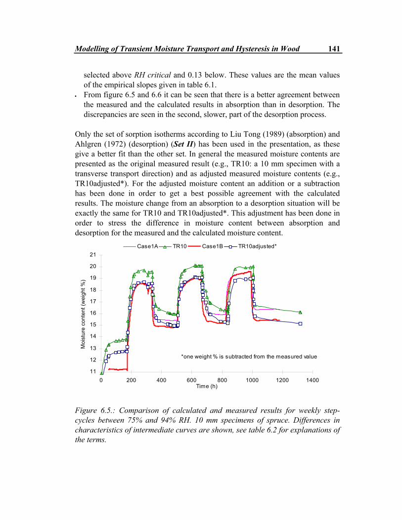
Modelling of Transient Moisture Transport and Hysteresis in Wood 141
selected above RH critical and 0.13 below. These values are the mean values of the empirical slopes given in table 6.1.
• From figure 6.5 and 6.6 it can be seen that there is a better agreement between the measured and the calculated results in absorption than in desorption. The discrepancies are seen in the second, slower, part of the desorption process.
Only the set of sorption isotherms according to Liu Tong (1989) (absorption) and Ahlgren (1972) (desorption) (Set II) has been used in the presentation, as these give a better fit than the other set. In general the measured moisture contents are presented as the original measured result (e.g., TR10: a 10 mm specimen with a transverse transport direction) and as adjusted measured moisture contents (e.g., TR10adjusted*). For the adjusted moisture content an addition or a subtraction has been done in order to get a best possible agreement with the calculated results. The moisture change from an absorption to a desorption situation will be exactly the same for TR10 and TR10adjusted*. This adjustment has been done in order to stress the difference in moisture content between absorption and desorption for the measured and the calculated moisture content.
11
12
13
14
15
16
17
18
19
20
21
0 200 400 600 800 1000 1200 1400Time (h)
Moi
stur
e co
nten
t (w
eigh
t %)
Case1A TR10 Case1B TR10adjusted*
*one weight % is subtracted from the measured value
Figure 6.5.: Comparison of calculated and measured results for weekly step-cycles between 75% and 94% RH. 10 mm specimens of spruce. Differences in characteristics of intermediate curves are shown, see table 6.2 for explanations of the terms.
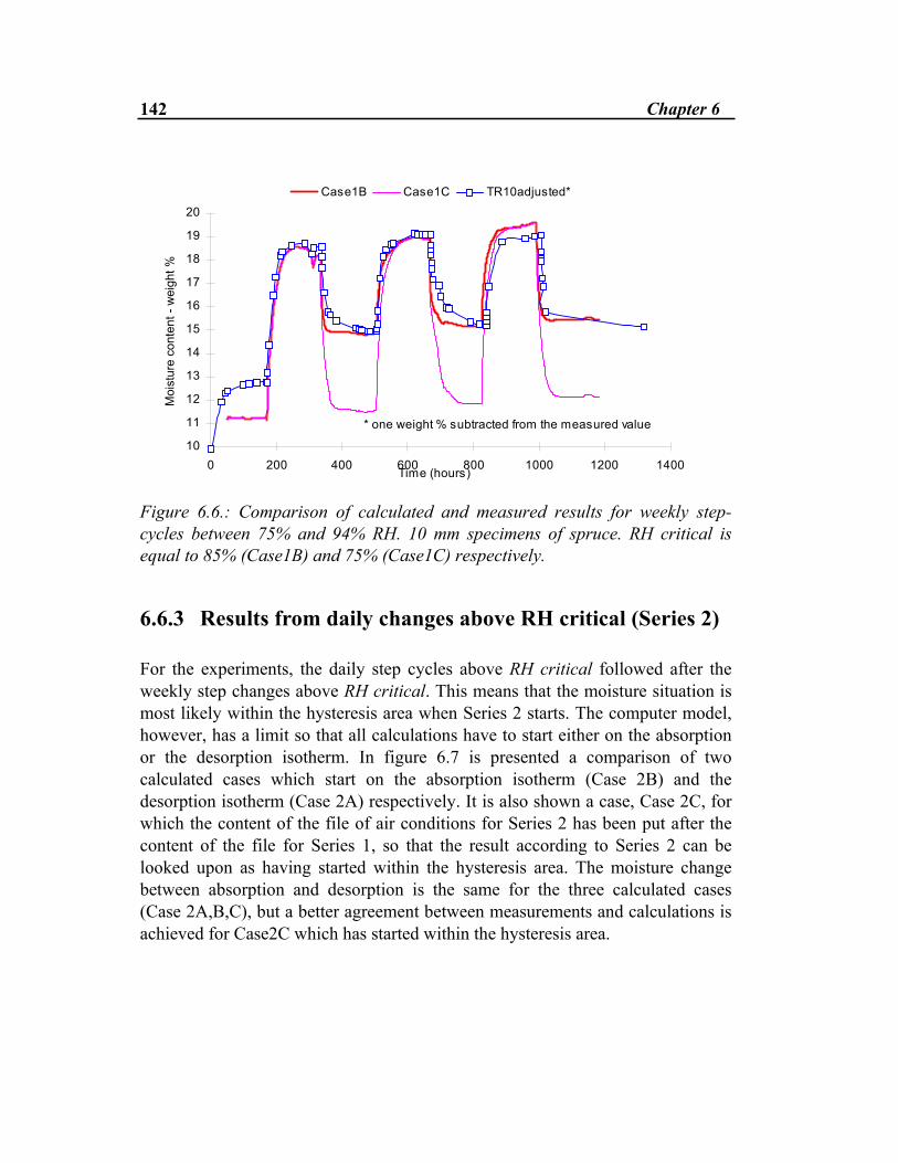
142 Chapter 6
10
11
12
13
14
15
16
17
18
19
20
0 200 400 600 800 1000 1200 1400Time (hours)
Moi
stur
e co
nten
t - w
eigh
t %
Case1B Case1C TR10adjusted*
* one weight % subtracted from the measured value
Figure 6.6.: Comparison of calculated and measured results for weekly step-cycles between 75% and 94% RH. 10 mm specimens of spruce. RH critical is equal to 85% (Case1B) and 75% (Case1C) respectively.
6.6.3 Results from daily changes above RH critical (Series 2) For the experiments, the daily step cycles above RH critical followed after the weekly step changes above RH critical. This means that the moisture situation is most likely within the hysteresis area when Series 2 starts. The computer model, however, has a limit so that all calculations have to start either on the absorption or the desorption isotherm. In figure 6.7 is presented a comparison of two calculated cases which start on the absorption isotherm (Case 2B) and the desorption isotherm (Case 2A) respectively. It is also shown a case, Case 2C, for which the content of the file of air conditions for Series 2 has been put after the content of the file for Series 1, so that the result according to Series 2 can be looked upon as having started within the hysteresis area. The moisture change between absorption and desorption is the same for the three calculated cases (Case 2A,B,C), but a better agreement between measurements and calculations is achieved for Case2C which has started within the hysteresis area.
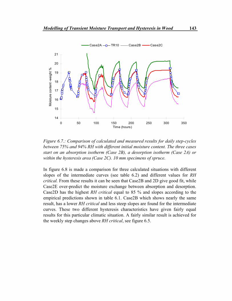
Modelling of Transient Moisture Transport and Hysteresis in Wood 143
14
15
16
17
18
19
20
21
0 50 100 150 200 250 300 350Time (hours)
Moi
stur
e co
nten
t -w
eigh
t %Case2A TR10 Case2B Case2C
Figure 6.7.: Comparison of calculated and measured results for daily step-cycles between 75% and 94% RH with different initial moisture content. The three cases start on an absorption isotherm (Case 2B), a desorption isotherm (Case 2A) or within the hysteresis area (Case 2C). 10 mm specimens of spruce. In figure 6.8 is made a comparison for three calculated situations with different slopes of the intermediate curves (see table 6.2) and different values for RH critical. From these results it can be seen that Case2B and 2D give good fit, while Case2E over-predict the moisture exchange between absorption and desorption. Case2D has the highest RH critical equal to 85 % and slopes according to the empirical predictions shown in table 6.1. Case2B which shows nearly the same result, has a lower RH critical and less steep slopes are found for the intermediate curves. These two different hysteresis characteristics have given fairly equal results for this particular climatic situation. A fairly similar result is achieved for the weekly step changes above RH critical, see figure 6.5.
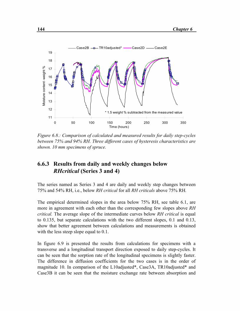
144 Chapter 6
11
12
13
14
15
16
17
18
19
0 50 100 150 200 250 300 350Time (hours)
Moi
stur
e co
nten
t -w
eigh
t %Case2B TR10adjusted* Case2D Case2E
* 1.5 weight % subtracted from the measured value
Figure 6.8.: Comparison of calculated and measured results for daily step-cycles between 75% and 94% RH. Three different cases of hysteresis characteristics are shown. 10 mm specimens of spruce.
6.6.3 Results from daily and weekly changes below RHcritical (Series 3 and 4) The series named as Series 3 and 4 are daily and weekly step changes between 75% and 54% RH, i.e., below RH critical for all RH criticals above 75% RH. The empirical determined slopes in the area below 75% RH, see table 6.1, are more in agreement with each other than the corresponding few slopes above RH critical. The average slope of the intermediate curves below RH critical is equal to 0.135, but separate calculations with the two different slopes, 0.1 and 0.13, show that better agreement between calculations and measurements is obtained with the less steep slope equal to 0.1. In figure 6.9 is presented the results from calculations for specimens with a transverse and a longitudinal transport direction exposed to daily step-cycles. It can be seen that the sorption rate of the longitudinal specimens is slightly faster. The difference in diffusion coefficients for the two cases is in the order of magnitude 10. In comparison of the L10adjusted*, Case3A, TR10adjusted* and Case3B it can be seen that the moisture exchange rate between absorption and
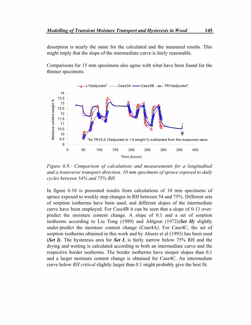
Modelling of Transient Moisture Transport and Hysteresis in Wood 145
desorption is nearly the same for the calculated and the measured results. This might imply that the slope of the intermediate curve is fairly reasonable. Comparisons for 15 mm specimens also agree with what have been found for the thinner specimens.
99.510
10.511
11.512
12.513
13.514
0 50 100 150 200 250 300 350 400
Time (hours)
Moi
stur
e co
nten
t wei
ght %
L10adjusted* Case3A Case3B TR10adjusted*
*for TR10-/L10adjusted is 1.5 weight % subtracted from the measured value
Figure 6.9.: Comparison of calculations and measurements for a longitudinal and a transverse transport direction. 10 mm specimens of spruce exposed to daily cycles between 54% and 75% RH. In figure 6.10 is presented results from calculations of 10 mm specimens of spruce exposed to weekly step changes in RH between 54 and 75%. Different sets of sorption isotherms have been used, and different slopes of the intermediate curve have been employed. For Case4B it can be seen that a slope of 0.13 over-predict the moisture content change. A slope of 0.1 and a set of sorption isotherms according to Liu Tong (1989) and Ahlgren (1972)(Set II) slightly under-predict the moisture content change (Case4A). For Case4C, the set of sorption isotherms obtained in this work and by Absetz et al (1993) has been used (Set I). The hysteresis area for Set I, is fairly narrow below 75% RH and the drying and wetting is calculated according to both an intermediate curve and the respective border isotherms. The border isotherms have steeper slopes than 0.1 and a larger moisture content change is obtained for Case4C. An intermediate curve below RH critical slightly larger than 0.1 might probably give the best fit.
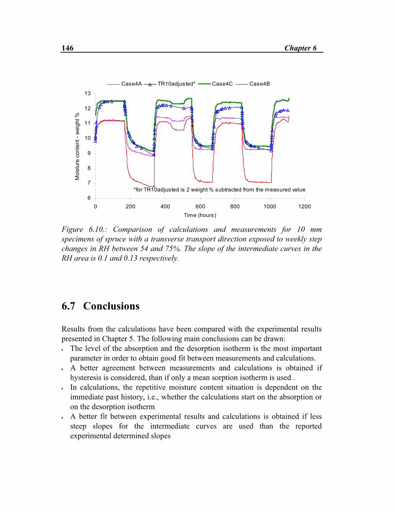
146 Chapter 6
6
7
8
9
10
11
12
13
0 200 400 600 800 1000 1200Time (hours)
Moi
stur
e co
nten
t - w
eigh
t %Case4A TR10adjusted* Case4C Case4B
*for TR10adjusted is 2 weight % subtracted from the measured value
Figure 6.10.: Comparison of calculations and measurements for 10 mm specimens of spruce with a transverse transport direction exposed to weekly step changes in RH between 54 and 75%. The slope of the intermediate curves in the RH area is 0.1 and 0.13 respectively.
6.7 Conclusions Results from the calculations have been compared with the experimental results presented in Chapter 5. The following main conclusions can be drawn: • The level of the absorption and the desorption isotherm is the most important
parameter in order to obtain good fit between measurements and calculations. • A better agreement between measurements and calculations is obtained if
hysteresis is considered, than if only a mean sorption isotherm is used . • In calculations, the repetitive moisture content situation is dependent on the
immediate past history, i.e., whether the calculations start on the absorption or on the desorption isotherm
• A better fit between experimental results and calculations is obtained if less steep slopes for the intermediate curves are used than the reported experimental determined slopes

Modelling of Transient Moisture Transport and Hysteresis in Wood 147
As an approach to modelling the sorption of wood exposed cyclic environmental changes, the model has proved to be rather promising. The shape of the measured and the calculated curves presented in this work corresponds very well. This could imply that application of linear intermediate curves, based on empirical data, could be a suitable way of modelling moisture hysteresis in wood.

148 Chapter 6

Chapter 7
Use of a Modified Timber Drying Apparatus for Sorption in Spruce
Part 1 - Experiments A new timber drying apparatus has been used for sorption measurements on spruce (Picea abies). A description of the apparatus has been made and the performance of the apparatus has been evaluated. Results from experiments where specimens from spruce have been exposed to changes in relative humidity and temperature are presented. 7.1 Introduction A new timber drying apparatus, designed and built at Department of Chemical and Process Engineering at University of Canterbury, New Zealand was modified and used for sorption measurements. The drying apparatus was originally
150 Chapter 7
constructed to facilitate drying experiments on timbers, such as Hard Beech (Nothofagus truncata) and Red Beech (Nothofagus fusca), which are known to be very difficult to dry and often suffer extensive degradation (damage) during drying. A more detailed description of the construction of the equipment can be found in Dakin (1996) or Time (1997). The apparatus has a modular structure of design so that it can easily be dismantled or additions can be made without much effort. This allows the equipment to be used for a variety of experimental work. For this project a cooler unit has been added to the apparatus to provide for lower temperatures. Sorption experiments on wood are often based on gravimetric methods. Traditional experiments of such kind often require manual weighings, and are in that sense very labour intensive. A more flexible and efficient method for sorption measurements such as offered by this particular apparatus would be of great importance for research societies. 7.2 Description of the small timber drying chamber
7.2.1 The packed column humidifier The humidification of the air is achieved by using a packed column (see figure 7.1 and 7.2) in which water is counter-currently contacted with air. The saturated air, coming from the packed column, is lead through a pipe, where it might be heated and dried before it goes into the actual drying section where the test specimen is hanging. The air is led out of the chamber in a pipe and exhausts outside the building. A packed column is a way of humidifying air which is generally called "wetted element humidification". This process basically involves water running over the surface of a packing or particle element being contacted with an air flow, see figure 7.2. The water running over the packing is coming from the tank underneath the packed column. The water is pumped from the tank through a pipe to the top of the column, where it is distributed to the packing through a distribution plate. Air from a compressor (Roots blower) is led into the bottom of the packed column.
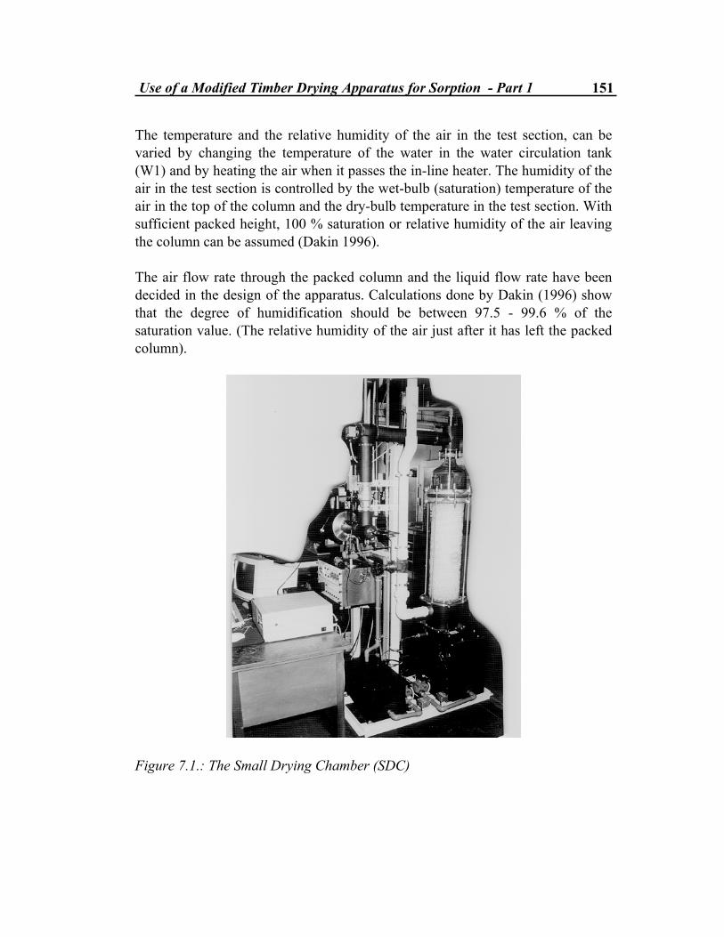
Use of a Modified Timber Drying Apparatus for Sorption - Part 1 151
The temperature and the relative humidity of the air in the test section, can be varied by changing the temperature of the water in the water circulation tank (W1) and by heating the air when it passes the in-line heater. The humidity of the air in the test section is controlled by the wet-bulb (saturation) temperature of the air in the top of the column and the dry-bulb temperature in the test section. With sufficient packed height, 100 % saturation or relative humidity of the air leaving the column can be assumed (Dakin 1996). The air flow rate through the packed column and the liquid flow rate have been decided in the design of the apparatus. Calculations done by Dakin (1996) show that the degree of humidification should be between 97.5 - 99.6 % of the saturation value. (The relative humidity of the air just after it has left the packed column).
Figure 7.1.: The Small Drying Chamber (SDC)

152 Chapter 7
���������������������
��������������
����������������������
������������
������������
��������������������������
�������������
�����������������
!�����������������
"�����������
#�������
�$��������
������������
%�����������
&����������� ����������� Figure 7.2.: The Small Drying Chamber; the packed column humidifier and the test section. Part of figure adapted from Dakin (1996).
7.2.2 Water heating and cooling The packed column is placed on top of a stainless steel tank (of about 40 litres) as shown in figure 7.1 and 7.2. The water tank (W1) provides the water for the humidification of the air. The tank was originally provided with heating only. It is designed for temperatures up to 70°C and also insulated with a closed-cell expanded foam, in order to reduce heat loss.
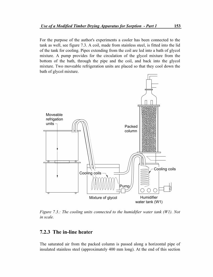
Use of a Modified Timber Drying Apparatus for Sorption - Part 1 153
For the purpose of the author's experiments a cooler has been connected to the tank as well, see figure 7.3. A coil, made from stainless steel, is fitted into the lid of the tank for cooling. Pipes extending from the coil are led into a bath of glycol mixture. A pump provides for the circulation of the glycol mixture from the bottom of the bath, through the pipe and the coil, and back into the glycol mixture. Two moveable refrigeration units are placed so that they cool down the bath of glycol mixture.
'�(���������������������
�����������
'�$��������)���
&���
&�����������
����������������������
�����������
Figure 7.3.: The cooling units connected to the humidifier water tank (W1). Not in scale.
7.2.3 The in-line heater The saturated air from the packed column is passed along a horizontal pipe of insulated stainless steel (approximately 400 mm long). At the end of this section
154 Chapter 7
there is an in-line heater, see figure 7.2, which provides for the right dry-bulb temperature and the relative humidity. The in-line heater is designed to heat the humidified air to a maximum of 80°C.
7.2.4 The test section The test section can be seen in figure 7.2 and 7.4. It is a 310 mm long tube with an internal diameter of 125 mm. The test section is operated adiabaticly1 to avoid condensation or cooling of the water vapour. A jacket2 was provided to meet that requirement. The diameter of the test section had to be made fairly small because it should be operated under vacuum. A larger diameter would have meant thicker walls and higher material costs. It was also necessary to keep the diameter small to reduce excessive air flow costs, as high air flows would mean that more energy was required for humidification. This had to be balanced against the necessity of having a diameter that provided adequate flow around the specimen and space so that the specimen could be placed in the test section (also called kiln or drying chamber) without too much difficulties. The test section has been insulated in order to reduce heat loss from the jacket. The test section might be put under vacuum by closing two valves on either side of the test section. The vacuum pump is connected to the test section by a third pipe. The vacuum pressure is manually controlled by a valve on the extension of the third pipe and observed on a pressure gauge. Only the test section has been designed to operate under vacuum pressure, the packed column and the water tank have not. This means that the test section has to be properly sealed and no air can go through under operation. Weighing of the specimen inside the test section goes on continuously and a weighing unit is installed on top of the test section, see figure 7.4. A small load cell is used to measure the weight of the specimen in the test section. A loadcell is basically a set of 4 strain gauges, the strain gauge measurements are converted to a current output, which is then amplified and converted to a Volt signal which is sent to the computer. The software program allows the input to be scaled and produces a weight value as an output (Dakin 1996). The main reasons 1 A process in which there is no heat transfer is called an adiabatic process . From Sonntag (1991). 2 A Jacket- An outer casing or cover surrounding an apparatus or a cylinder, the space inside the jacket filled with a cooling or heating fluid or with insulation material. From Lydersen and Dahloe (1992).
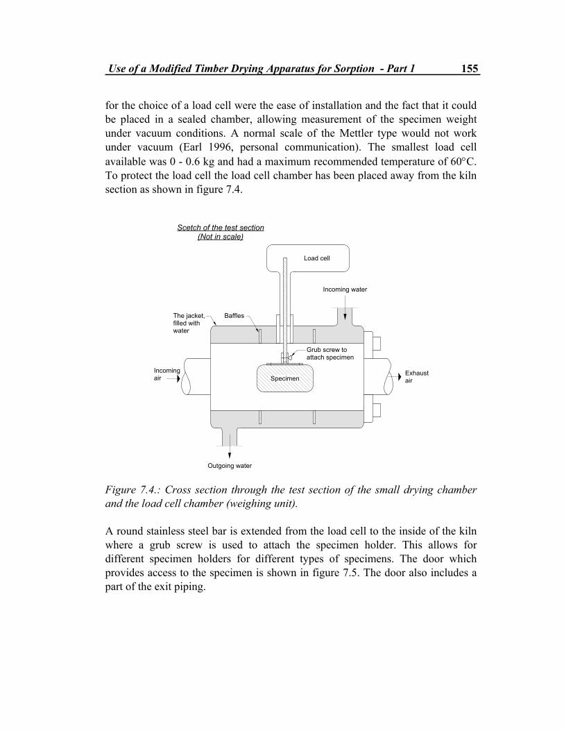
Use of a Modified Timber Drying Apparatus for Sorption - Part 1 155
for the choice of a load cell were the ease of installation and the fact that it could be placed in a sealed chamber, allowing measurement of the specimen weight under vacuum conditions. A normal scale of the Mettler type would not work under vacuum (Earl 1996, personal communication). The smallest load cell available was 0 - 0.6 kg and had a maximum recommended temperature of 60°C. To protect the load cell the load cell chamber has been placed away from the kiln section as shown in figure 7.4.
������������������������ ����������
*���������+�����,�������������
%�������
#�������
"�����������������������
�����������
-�����������
������������
�$��������
Figure 7.4.: Cross section through the test section of the small drying chamber and the load cell chamber (weighing unit). A round stainless steel bar is extended from the load cell to the inside of the kiln where a grub screw is used to attach the specimen holder. This allows for different specimen holders for different types of specimens. The door which provides access to the specimen is shown in figure 7.5. The door also includes a part of the exit piping.

156 Chapter 7
Figure 7.5.: The door in the test section.
7.2.5 The design of the kiln jacket for adiabatic conditions A jacket on the test section is used for adiabatic conditions, see figure 7.4. The test section cylinder contains an inner and an outer wall. Baffles are installed to provide an even flow of water around the test section in order to avoid cold spots. The jacket is fed by water from a water tank (W2) and a circulation pump. A cooler coil is installed in the tank if cooling is necessary.
7.2.6 Control and instrumentation The humidity is controlled by manipulation of the heat input to the water in the water tank (W1) to give the desired saturation temperature at the top of the column. The temperature at the top of the column is measured using a Platinum Resistance Thermometer (PRT). A PRT is a thin layer of platinum on a ceramic backing. The platinum has been laser-trimmed to give the correct output of resistance versus temperature. A PRT is used as it is considerably more accurate than a thermocouple and it produces a linear output versus temperature. The output from the PRT is converted to a voltage signal which is transmitted to the computer. Two PRT's are used, one for the dry-bulb temperature (Tdry) in the inlet to the actual test section (see figure 7.6) and one for the wet bulb temperature (Twet) at the top of the column. The output temperatures, which are logged by the control software are the wet bulb temperature (saturation
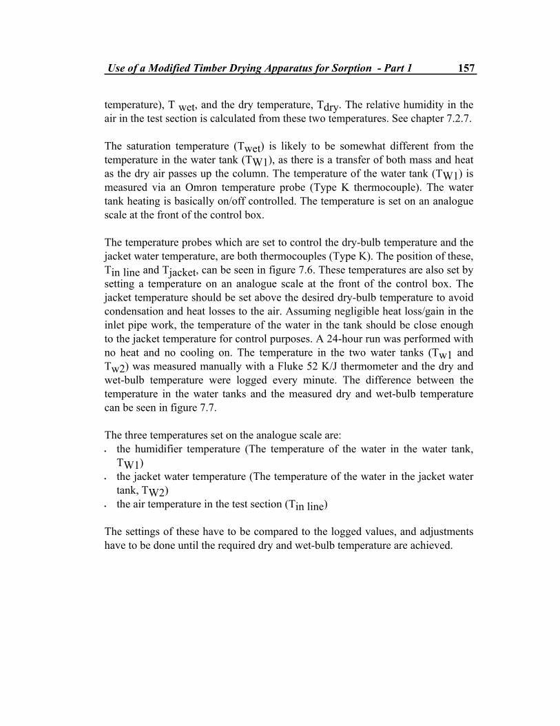
Use of a Modified Timber Drying Apparatus for Sorption - Part 1 157
temperature), T wet, and the dry temperature, Tdry. The relative humidity in the air in the test section is calculated from these two temperatures. See chapter 7.2.7. The saturation temperature (Twet) is likely to be somewhat different from the temperature in the water tank (TW1), as there is a transfer of both mass and heat as the dry air passes up the column. The temperature of the water tank (TW1) is measured via an Omron temperature probe (Type K thermocouple). The water tank heating is basically on/off controlled. The temperature is set on an analogue scale at the front of the control box. The temperature probes which are set to control the dry-bulb temperature and the jacket water temperature, are both thermocouples (Type K). The position of these, Tin line and Tjacket, can be seen in figure 7.6. These temperatures are also set by setting a temperature on an analogue scale at the front of the control box. The jacket temperature should be set above the desired dry-bulb temperature to avoid condensation and heat losses to the air. Assuming negligible heat loss/gain in the inlet pipe work, the temperature of the water in the tank should be close enough to the jacket temperature for control purposes. A 24-hour run was performed with no heat and no cooling on. The temperature in the two water tanks (Tw1 and Tw2) was measured manually with a Fluke 52 K/J thermometer and the dry and wet-bulb temperature were logged every minute. The difference between the temperature in the water tanks and the measured dry and wet-bulb temperature can be seen in figure 7.7. The three temperatures set on the analogue scale are: • the humidifier temperature (The temperature of the water in the water tank,
TW1) • the jacket water temperature (The temperature of the water in the jacket water
tank, TW2) • the air temperature in the test section (Tin line) The settings of these have to be compared to the logged values, and adjustments have to be done until the required dry and wet-bulb temperature are achieved.
158 Chapter 7
��.����������
&������������
��� ,���������)&/�������
���.���� ,���������)������������������������)
���.���� &/�0�����������������������������
#�������
�����������
���)
���������)&/�������
�� ���������)������������������������
� ���������)�����������������1����������
%�����������
�$��������
���� �� �
������������������
2�������������
Figure 7.6.: A schematic drawing of the different temperatures measured and controlled (not in scale).

Use of a Modified Timber Drying Apparatus for Sorption - Part 1 159
0
5
10
15
20
25
30
35
0 20000 40000 60000 80000 100000Time (s)
Tem
pera
ture
(C)
Tsat Tdry T jacket water T humidifier
Ambient temperature 22 CStart at 9 a.m
Figure 7.7.: Temperature development in the water tanks (TW1 =Thumidifier and TW2 =Tjacket water ), in test section (Tdry) and in top of the packed column (Tsat) when there is no heat nor cooling on.
7.2.7 Software The ADVANTECH Genie Data Acquisition and Control Software (Advantech 1993) is used to log the wet-bulb (Twet ) and the dry-bulb (Tdry ) temperature and the weight of the specimen. The Genie Software provides an icon-based, mouse-driven system for designing real-time automation and control strategies. Dakin (1996) made a user program to convert the wet-bulb depression into a relative humidity. This, in addition to the weight of the specimen, the wet-bulb (Twet) and the dry-bulb (Tdry) temperature, are displayed on a screen when performing an experiment and running the software program. Calculation of the Relative Humidity in the Test Section The relative humidity of the air in the test section as calculated by Dakin (1996) is not correct in relation to the actual mass and heat processes happening. The relative humidity in the test section should be calculated in the following way. Twet and Tdry are measured values ( °C). The basic equation for the relative humidity is

160 Chapter 7
RH pps
= ⋅100 [%] (7.1)
where ps is the saturation pressure at the dry-bulb temperature. Further, the saturation pressure over liquid water for the temperature range of 0 to 200 °C is given by (ASHRAE 1989): ln( ) /p A T B T Ts dry dry dry= + + ⋅ + ⋅ + ⋅ + ⋅ C T D E F ln(T )dry dry
2 3 [Pa] (7.2) where A, B, C, D, E and F are constants, see ASHRAE (1989). Corresponding for p ln( ) /p A T B T Twet wet wet= + + ⋅ + ⋅ + ⋅ + ⋅ C T D E F ln(T )wet wet
2 3 [Pa] (7.3)
7.2.8 Calculation of air velocity in the test section The air velocity in the test section is controlled through a valve, and it has to be set manually. The air velocity is measured with an orifice flow meter positioned in the exhaust pipe. The orifice meter is connected to a manometer, which measures the pressure drop across the orifice. See figure 7.8. The following approximate equation, given in McCabe et al. (1993), has been proposed by the author for calibration so that the velocity in the exhaust pipe can be calculated.
u C P Pa b0
041
2=
−⋅
⋅ −
β ρ( )
(7.4)
where u0 = the velocity through the orifice (m⋅s-1) β = ratio of the orifice diameter to the pipe diameter Pa,Pb = pressures at position a and b in figure 7.9 a) (Pa) ρ = density of the fluid (kg⋅m-3) C0 is the orifice coefficient. It corrects for the contraction of the fluid jet between the orifice and the vena contracta and for friction; it always has to be determined experimentally. C0 varies considerably with changes in β and with Reynolds

Use of a Modified Timber Drying Apparatus for Sorption - Part 1 161
number at the orifice. Reynolds numbers ranging from approximately 2500 - 20 000 are found in this work. Velocities for pressure drops between 5 and 125 Pa have been measured. Because the Reynolds number is below 30 000 for all velocities the coefficient C0 has to be calculated each time. Figure 7.8 gives C0 as a function of pressure drop ∆P.
a)
b)
y = 2E-10x5 - 1E-07x4 + 2E-05x3 - 0.0013x2 + 0.0441x + 0.1422R2 = 0.9824
0
0.1
0.2
0.3
0.4
0.5
0.6
0.7
0 20 40 60 80 100 120 140Delta P (Pa)
C -
orifi
ce c
oeffi
cien
t
C evaluated from measurements Poly. (C evaluated from measurements)
Figure 7.8.: a) Orifice meter (adapted from McCabe et al. 1993)
b) The orifice coefficient, C0, as a function of pressure drop across the orifice. The equation for a polynomial fit is given.
On assuming continuity in the air flow throughout the whole system, the following simple continuity equation can be set up
162 Chapter 7
Q u A u ASDC SDC= ⋅ = ⋅0 0 (7.5) where Q = air flow (m3⋅s-1 )
u−
0 = average velocity through the orifice plate (m⋅s-1 )
uSDC
−
= average velocity through the test section of the small drying chamber (m⋅s-1 ) A0 = cross section area of the orifice plate (vena contracta) (m2 ) ASDC = cross section area of the interior of the small drying chamber (m2) From this equation an approximate air velocity through the test section of the Small Drying Chamber (SDC) can be set up. During the sorption measurements the air velocity in the test section has been kept at approximately 0.1 - 0.3 m⋅s-1.
7.2.9 Experiences with the apparatus performing sorption measurements Air Conditions When the cooling units were first installed, they were meant to provide for lowering the temperature below ambient. But while using the SDC without cooling I experienced that quite a lot of heat was developed in the system due to water circulating through two pumps (from water tank W1 through the packed column and from water tank W2 to the jacket). As a result of this the lowest possible dry-bulb temperature that could be obtained with no extra cooling and an ambient temperature of 20°C was approximately 30°C. This means that to be able to run the apparatus below 30°C cooling has to be provided, and that the cooler is needed to provide for the temperature to be lowered down to ambient. The SDC was left running with the coolers on to find out what were the lowest obtainable temperatures. The system had come to an equilibrium after 12 hours. Then the dry-bulb temperature (Tdry) was 10.5°C and the temperature at the outlet of the packed column was 14.0°C. The ambient temperature during that 12- hour period was around 20°C. This means that the lowest practicable dry-bulb temperature is about 15 - 16°C. Only the heaters of the two water tanks (WT1 and WT2) and the in-line heater are controlled, there is no automatically control of the coolers. They have to be manually switched on and off. When no heating is required the temperatures

Use of a Modified Timber Drying Apparatus for Sorption - Part 1 163
(Tdry and Twet) will, apart from being dependent on the water temperatures, also be dependent on the temperature of the incoming air and the ambient temperature (heat is transferred from the packed column to the room). This makes it difficult to keep stable conditions at low temperatures (around ambient). The Canterbury region is exposed to rapid changes in temperature. As an example; on January 21 in 1997 the temperature dropped from 30 °C to 16 °C within 1 hour. For an apparatus like the SDC to be well suitable for sorption measurements at temperatures below and around ambient the incoming air should be cooled before being mixed with the cooled water, the cooler should be automatically controlled and the packed column should have been insulated. Another, but some more complex solution, would have been to cool the air down after it had passed the packed column. For more easily and accurately setting the temperatures, they should have been able to set on a digital scale. When only a small shift in temperature is wanted, this can be quite hard to obtain on the analogue scale. Condensation has appeared to be a problem at the ends of the test section at higher dry-bulb temperatures (Keey 1997, personal communication). The author also observed condensate at the bottom of the chamber when opening the chamber after having finished the last experiment. As there is a drain in the chamber and relatively long-time experiments have been performed, it is difficult to tell anything about the amount of condensation. Weight measurements Weighing of the test specimen in the SDC is done by using a load cell. Test performances done with only the specimen holder mounted to the bar from the load cell showed fairly large differences in weight recordings. Two main reasons for this are reported by Dakin (1996): firstly, the signal from the load cell is subject to electrical noise which is partly due to the load cell amplifier; secondly, the specimen weight recorded is subject to fluctuations in weight due to fluctuations in air velocity. This is more prominent at high air velocities. To obtain a better performance from the load cell, the logged values of the weight of the specimen (1 logging every 60 seconds) have been based on an average of 100 scans (1 scan per second). The experiments were performed under very low air velocities (0.1-0.3 ms-1) and the influence of the air to the weight fluctuations is hardly noticeable (a fairly light specimen on a rigid steel bar). The weight of the specimen was measured on a scale immediately before it was placed in the
164 Chapter 7
chamber. There was no significant difference between the weight of the specimen outside and inside with the air flowing through. According to the Load Cell Calibration Certificate, the largest inaccuracy which can be obtained for the load cell is 0.3 grams of full scale (FS) (FS is 600 grams). This is if, creep, thermal shift and hysteresis all work in the same direction. The specimens with which I worked, have a weight at normal ambient conditions (room temperature and 60 % relative humidity) varying from about 15 grams to 30 grams. An error of 0.3 grams will correspond to an inaccuracy of 1 to 2 %. To reduce this error 4 specimens had to be hung in the SDC at a time. In that way the inaccuracy could be spread over several specimens. Another advantage by doing the experiment that way was that the differences between the different specimens were eliminated. During a period of two months, the load cell was calibrated 3 times, before the experiments started, in the middle of the period and after the experiments had finished. A drift of nearly 1 gram appeared over the whole period. This drift has been allowed for in the reported results. Vacuum Vacuum was tried employed to establish a moisture equilibrium level for the wooden specimens. This was abandoned because it was unsure what effect vacuum would actually have on the hygroscopicity and other material properties of wood. Another factor derives from the practice when shutting the valves to evacuate the test section, the humidity level inside the test section is not measured. The wet-bulb temperature is measured on top of the packed column and, in the absence of condensation, should yield the humidity level in the chamber. Comparison of two different kind of sorption apparatus The author has used two different kind of apparatus for sorption measurements on spruce. The Sorption Apparatus (SA) at the Department of Building and Construction Engineering is a simple construction principally made from two fairly large vessels, a lid construction containing up to 50 test specimens and a fan to obtain

Use of a Modified Timber Drying Apparatus for Sorption - Part 1 165
air circulation in the vessels, see Chapter 5. The required climate is obtained by storing the apparatus in a room with a fixed temperature, and saturated salt solutions are used to keep a certain relative humidity inside the vessels. The particular relative humidity which can be obtained from the specific saturated salt solutions and the temperature range available in the room where the vessels are placed put a limitation to the choice of a climate. The apparatus can contain up to 50 specimens at a time which are weighed manually on a Mettler scale. The weighing is done inside the apparatus. A more detailed description of the apparatus and results from these measurements can be found in Chapter 5. The Small Drying Chamber (SDC) at Department of Chemical and Process Engineering (CAPE) is a much more complex construction where the required conditions are obtained from mixing heated water and outdoor air in a humidifier ("wetted element humidification"). The saturated air from the mixture of water and air can thereafter be heated to obtain the right temperature and relative humidity. The apparatus was originally designed for drying of timber and should work in the range from ambient temperature up to 120°C. Cooling has been provided so that it should be possible to run for lower temperatures. Only one specimen can be in the chamber at a time, and it is weighed automatically using a load cell. A brief overview of the two principles of performing sorption measurements can be seen in table 7.1. The use of salt solutions has often been criticised because of the inherent uncertainties. Though it can be hard to obtain exact pre-defined RH-levels, a fixed relative humidity can be obtained, which is reasonably stable at a constant temperature level. (Some salt solutions are more temperature-stable than others). By use of relative humidity sensors above the saturated salt solutions, the RH-levels and the temperatures can be measured continuously, and at an acceptable degree of accuracy. The principle of the SDC is to obtain a fixed relative humidity by mixing water and air. The relative humidity is not measured directly, but it is calculated from the wet-bulb (saturation) and the dry-bulb temperatures. Measurements have shown that it is difficult to keep the relative humidity stable for temperatures around ambient. A more stable RH was obtained by use of the SA. The actual test section, where the experiments take place, is quite different for the two rigs. The test section of the SA is a big volume, while the test section of the
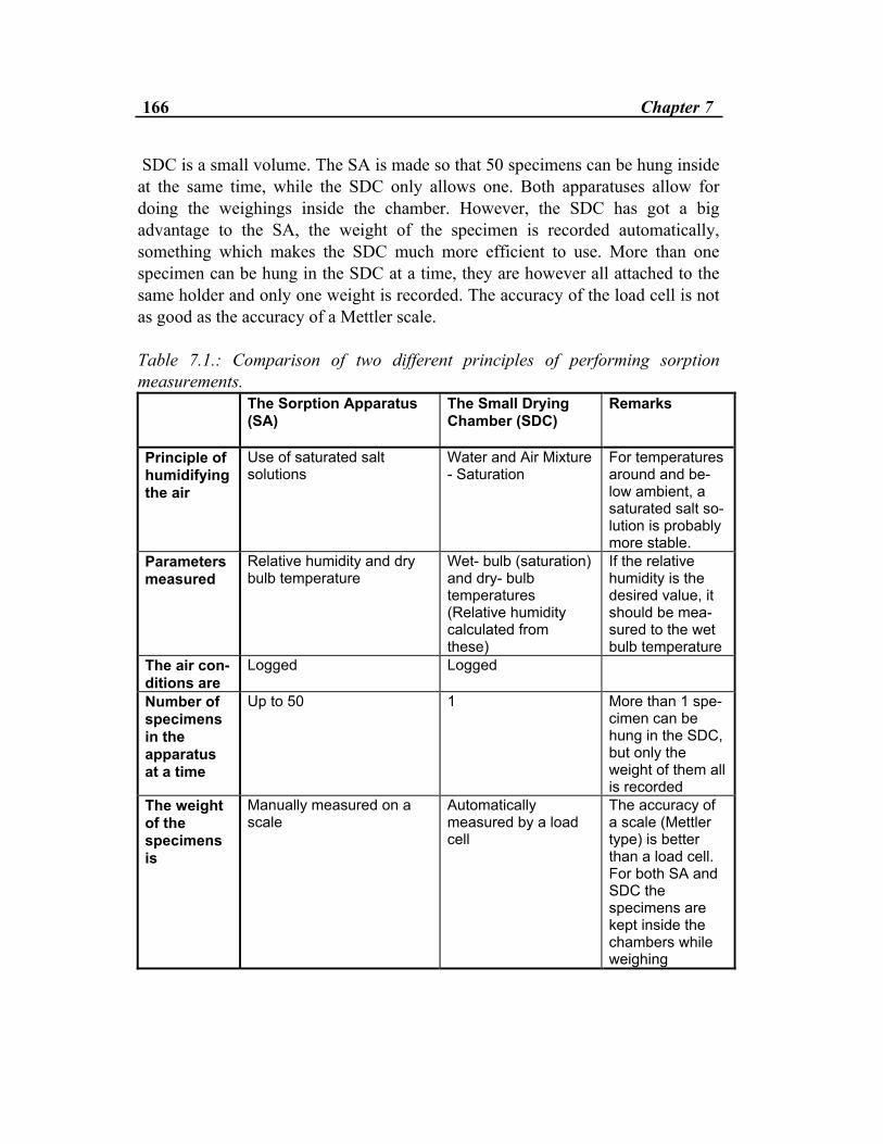
166 Chapter 7
SDC is a small volume. The SA is made so that 50 specimens can be hung inside at the same time, while the SDC only allows one. Both apparatuses allow for doing the weighings inside the chamber. However, the SDC has got a big advantage to the SA, the weight of the specimen is recorded automatically, something which makes the SDC much more efficient to use. More than one specimen can be hung in the SDC at a time, they are however all attached to the same holder and only one weight is recorded. The accuracy of the load cell is not as good as the accuracy of a Mettler scale. Table 7.1.: Comparison of two different principles of performing sorption measurements. The Sorption Apparatus
(SA)
The Small Drying Chamber (SDC)
Remarks
Principle of humidifying the air
Use of saturated salt solutions
Water and Air Mixture - Saturation
For temperatures around and be-low ambient, a saturated salt so-lution is probably more stable.
Parameters measured
Relative humidity and dry bulb temperature
Wet- bulb (saturation) and dry- bulb temperatures (Relative humidity calculated from these)
If the relative humidity is the desired value, it should be mea-sured to the wet bulb temperature
The air con-ditions are
Logged Logged
Number of specimens in the apparatus at a time
Up to 50 1 More than 1 spe-cimen can be hung in the SDC, but only the weight of them all is recorded
The weight of the specimens is
Manually measured on a scale
Automatically measured by a load cell
The accuracy of a scale (Mettler type) is better than a load cell. For both SA and SDC the specimens are kept inside the chambers while weighing
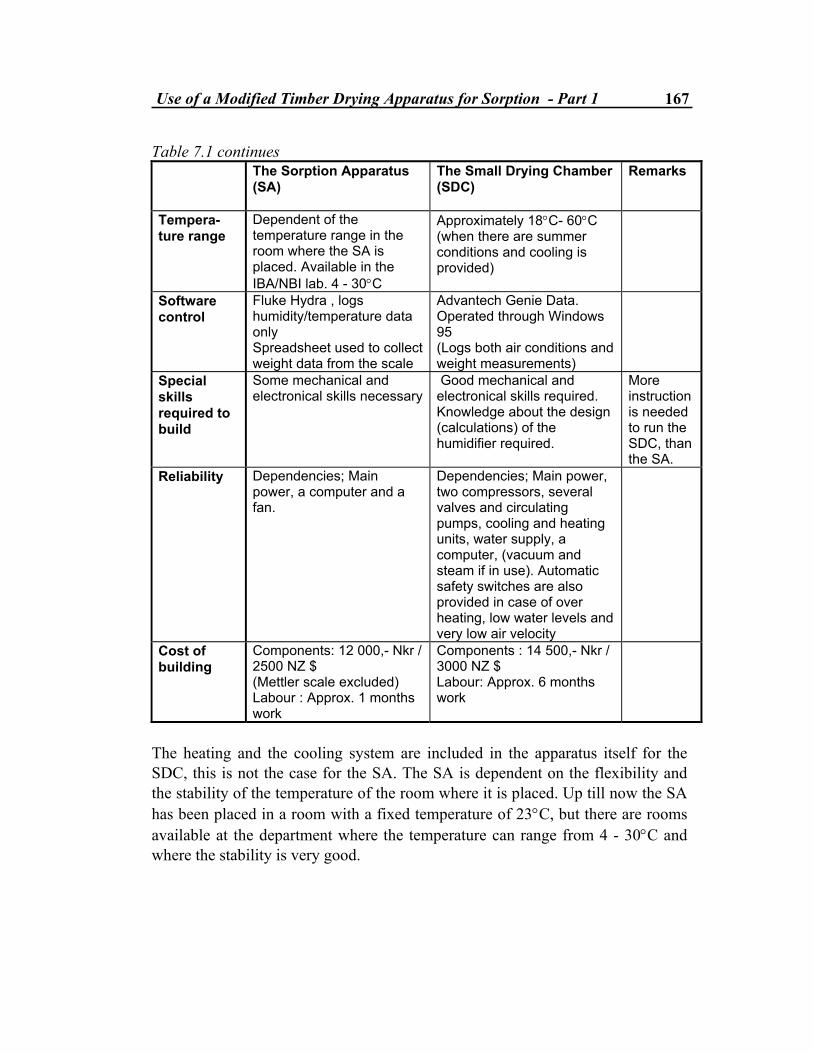
Use of a Modified Timber Drying Apparatus for Sorption - Part 1 167
Table 7.1 continues The Sorption Apparatus
(SA)
The Small Drying Chamber (SDC)
Remarks
Tempera-ture range
Dependent of the temperature range in the room where the SA is placed. Available in the IBA/NBI lab. 4 - 30°C
Approximately 18°C- 60°C (when there are summer conditions and cooling is provided)
Software control
Fluke Hydra , logs humidity/temperature data only Spreadsheet used to collect weight data from the scale
Advantech Genie Data. Operated through Windows 95 (Logs both air conditions and weight measurements)
Special skills required to build
Some mechanical and electronical skills necessary
Good mechanical and electronical skills required. Knowledge about the design (calculations) of the humidifier required.
More instruction is needed to run the SDC, than the SA.
Reliability Dependencies; Main power, a computer and a fan.
Dependencies; Main power, two compressors, several valves and circulating pumps, cooling and heating units, water supply, a computer, (vacuum and steam if in use). Automatic safety switches are also provided in case of over heating, low water levels and very low air velocity
Cost of building
Components: 12 000,- Nkr / 2500 NZ $ (Mettler scale excluded) Labour : Approx. 1 months work
Components : 14 500,- Nkr / 3000 NZ $ Labour: Approx. 6 months work
The heating and the cooling system are included in the apparatus itself for the SDC, this is not the case for the SA. The SA is dependent on the flexibility and the stability of the temperature of the room where it is placed. Up till now the SA has been placed in a room with a fixed temperature of 23°C, but there are rooms available at the department where the temperature can range from 4 - 30°C and where the stability is very good.
168 Chapter 7
The SA is a much more simple construction than the SDC, something which makes it easier to build. Only some mechanical and electronical skills are necessary. For the SDC, however, in addition to both good mechanical and electronical skills, knowledge about design of humidifiers is required. Both apparatuses can be run without special knowledge, but more instructions and safety precautions are needed when running the SDC. The reliability of the apparatuses is dependent on the different components they consist of. While the SA has very few components and in that sense has a high reliability, the SDC consists of more components which have to work independently and together. A fairly new and more flexible software control program is used with the SDC, something which makes it more easy to check and treat the collected data. The original purposes of the design of the two apparatuses with the complexity of the SDC and the simplicity of the SA were different. The SDC was set up to facilitate drying experiments on timber samples, while the SA was set up for the purpose of doing sorption measurements on small wooden pieces. 7.3 Sorption Measurements in the SDC
7.3.1 Objectives Quite a few experiments on sorption in wood have been performed throughout the years, but they have often been sorption measurements (see e.g. section 4.1) in order to evaluate diffusion coefficients. Basic research on moisture in wood exposed to changes in surrounding conditions are not widespread. One reason for this may be that it is very time-demanding to do such experiments. By the use of a gravimetric method frequent weighings have to be done. The principle described in this chapter could be a more efficient alternative to the more traditional gravimetric methods. The objective of this experiment has been to study the moisture performance of small specimens of wood exposed to relatively short lasting step changes in both relative humidity and temperature. The step changes were made after an apparent

Use of a Modified Timber Drying Apparatus for Sorption - Part 1 169
equilibrium situation was reached. If there were trouble in keeping the temperature and relative humidity stable the specimens were kept for a longer time at that particular step. Before the described experiments took place an initial drying experiment under steady state conditions was performed, to map the drying characteristics. 7.3.2 Selection and preparation of specimens Spruce, Picea abies, from central Norway, has been used in the experiments. Small clearwood specimens, taken near the pit, were cut (70 mm x 50 mm x 10 mm) and prepared in a rectangular shape with rounded corners. The specimens have all been prepared by sawing. The vapour transport should be one-dimensional so the specimens have been sealed at the edges. A very vapour-tight sealing paint used at CAPE, University of Canterbury and by the New Zealand Timber Industry has been used for sealing. (A two-component paint named Devshield 236, Altex Devoe). Four specimens have been screwed to the specimens' holder at a time, see figure 7.9. The specimen holder is connected to the steel bar extended from the load cell. All the specimens were resaturated by the use of a vacuum oven (a pressure corresponding to 0.8 atmospheres was obtained). After no more rapid water uptake could be obtained by the vacuum oven, the specimens were left in water for another month. A moisture content of about 140 - 160 weight % was obtained for all specimens.
Figure 7.9.: Four specimens screwed to the holder. Three sets of specimens have been used for the experiments, named set A, set B and set I. See table 7.2 for their characteristics

170 Chapter 7
Set of
Specimens** Transport Direction
Thickness of Specimen
Density
Used in Experiment*
Set I Radial 10 mm 400 kg⋅m-3 Initial drying exp. Set A Longitudinal 10 mm 355 kg⋅m-3 1 Set B Longitudinal 10 mm 350 kg⋅m-3 2,3,4
* See chapter 7.3.3 for explanation of the experiments. ** One set includes 4 specimens. Table 7.2 Characteristics of specimen
7.3.3 Performed experiments and air conditions The overall experiment can be divided into one initial drying experiment and thereafter four small sorption experiments. Two of these experiments have been repeated. The levels of the first two experiments were repeated because quite high moisture contents were observed especially at high temperatures. This means that the first and the third experiment were run at the same levels of relative humidity and temperature, so were the second and the fourth.
Experiment Duration Set of specimens
Initial Moisture Content
1 8 days A Fully saturated (~160 weight %) 2 11 days B Fully saturated (~160 weight %) 3 7 days B Final MC (weight %) for exp. 2 4 8 days B Final MC (weight %) for exp. 3
Table 7.3.: The initial condition of the specimens for the four different experiments.
Experiment Tdry (°C) Tsat (°C) Calculated RH (%) 23 22 94
1 and 3 30 24 70 40 27 48 23 17 70
2 and 4 30 20 55 40 23 38
Table 7.4.: The different levels of relative humidity and temperature used.

Use of a Modified Timber Drying Apparatus for Sorption - Part 1 171
The same temperature intervals were used for all four experiments. Each experiment lasted from one week to 11 days. Two different sets of test specimens have been used. Set A was used for experiment 1, while the same set B was used for the three following experiments. The objective for keeping the same sets of test specimens for the last three runs was to see if the high moisture content observed for the first experiment would decrease in the following experiments. The initial moisture content of the specimens for the four different experiments can be seen in table 7.3. The different levels of relative humidity and temperatures that were set are given in table 7.4. The problems with keeping the air conditions in the chamber stable, as discussed earlier, resulted in the variations shown in figure 7.12 to 7.15.
7.3.4 «Initial drying experiment» Research has shown that it may take a relatively long time to reach final equilibrium with the surrounding conditions when drying from saturated specimens. Before the experiments described above were started, a drying experiment was performed to study the drying curve for a nearly saturated set of specimens under steady-state conditions. The result from this experiment can be seen in figure 7.10. The curve is derived from three minute averages based on weight loggings every minute. Also the temperature and the relative humidity are based on the three-minute logging values. A set of specimens with one-dimensional transport in the radial direction has been used (Set I). The drying curve begins with a period of hardly any change in average moisture content for a period of 11 hours. A possible explanation for this is that there is a very big moisture gradient in a very thin surface layer, while a redistribution takes place in the interior layers because of the high permeability in the core. Because of this the average moisture content in the set of wood specimens is constant for the first period of time. See figure 7.11. The constant drying period with evaporation from the surface lasts approximately until the end of day 2; from day 2 to day 3 there is a further evaporation from the pores. All liquid seems to have disappeared between day 2 and 3. A moisture content level of 16,5 % has been reached after 6.5 days (156 hours).

172 Chapter 7
020406080
100120140160
0 20 40 60 80 100 120 140 160 180Time (h)
Moi
stur
e co
nten
t wei
ght (
%)
0102030405060708090100
Tem
p (C
)/ R
H (%
)
u % Tdry RH (%)
3 days "Square"
a)
Enlargement of "Square"
12141618202224
0 20 40 60 80 100 120 140 160 180
Time (h)
Moi
stur
e co
nten
t (w
eigh
t%)
0
20
40
60
80
100
Tem
p (C
)/ R
H (%
)
RH (%)
Temp (C)u (%)
b) Figure 7.10.: a) Drying curve for 10 mm spruce, 1 dimensional drying in the radial direction, b) Enlargement of the slow stage of the drying curve. This moisture level is suspiciously low; it is in the range of an absorption isotherm. As mentioned before, condensation might have happened in the drying chamber. This means that the calculated relative humidity might be too high. No condensate was seen when the chamber was opened, but the chamber has a drainage port and condensation might have happened sometimes during the six-day period. The weight of the set of specimens was checked on a Mettler balance just after the experiment had finished, and the weight at that stage was in accordance with the weight of the load cell. The low moisture content cannot be explained by the readings from the load cell.
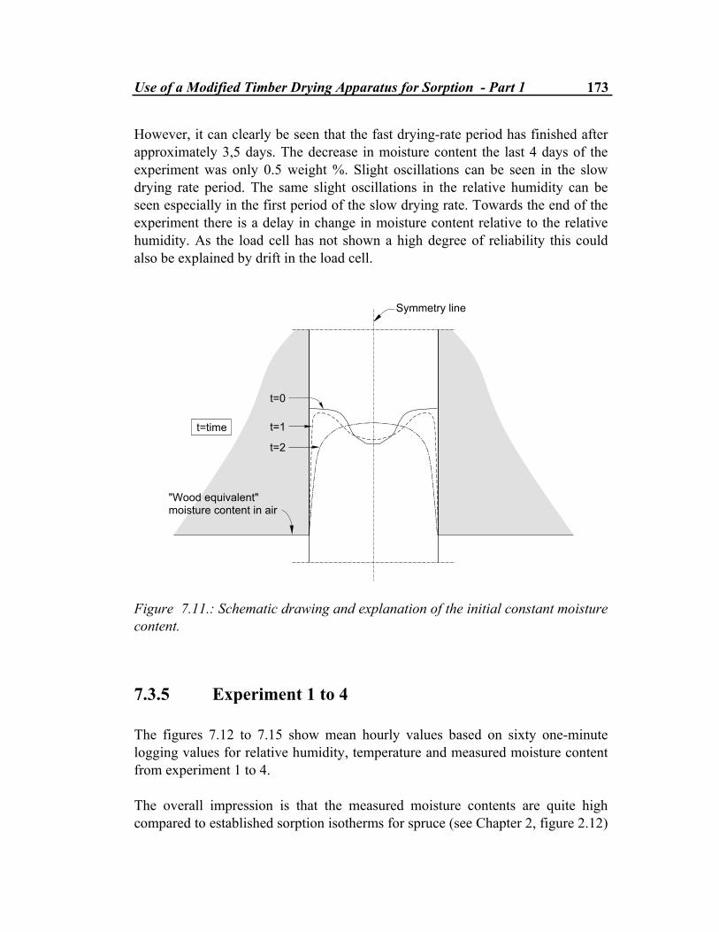
Use of a Modified Timber Drying Apparatus for Sorption - Part 1 173
However, it can clearly be seen that the fast drying-rate period has finished after approximately 3,5 days. The decrease in moisture content the last 4 days of the experiment was only 0.5 weight %. Slight oscillations can be seen in the slow drying rate period. The same slight oscillations in the relative humidity can be seen especially in the first period of the slow drying rate. Towards the end of the experiment there is a delay in change in moisture content relative to the relative humidity. As the load cell has not shown a high degree of reliability this could also be explained by drift in the load cell.
������������ ������������ �� �� ���
���������� �
���
���
���
�����
Figure 7.11.: Schematic drawing and explanation of the initial constant moisture content.
7.3.5 Experiment 1 to 4 The figures 7.12 to 7.15 show mean hourly values based on sixty one-minute logging values for relative humidity, temperature and measured moisture content from experiment 1 to 4. The overall impression is that the measured moisture contents are quite high compared to established sorption isotherms for spruce (see Chapter 2, figure 2.12)
174 Chapter 7
for all temperatures and relative humidities. Same set of specimens have been used for 3 following experiments to see if lower moisture contents were obtained. A rather small decrease was observed and the moisture contents were still quite high. The uncertainty around establishing the relative humidity (see previous chapter) might be an explanation for the high level of moisture contents. The relative humidity might have been calculated too low. Calculations which take this into account are presented in Chapter 8. For experiment 1 (figure 7.12) vacuum was set on the drying chamber to increase the drying rate. As can be seen from the moisture content curve in figure 7.12, there was a strong weight increase just after the vacuum was taken off although the temperature was rising. Because of this the temperature was turned down again and a temperature of 23°C was kept until the moisture content has started levelling out. Overall, it can be seen that the set of 10-mm longitudinal specimens reacts rather fast when there is a change in relative humidity. A smaller, but not lasting change does not seem to affect the moisture content very much (see e.g. figure 7.12 after 145 hours). However, a rather small, but lasting change seem to have a lasting effect (e.g., see figure 7.15 after 40 hours). This has also been observed in the experiments presented in Chapter 5. The sorption rates, both absorption and desorption, respond rapidly for all the planned step changes. A more fluctuating step change (relative humidity and temperature) gives a slower sorption rate (e.g. first desorption in experiment 2 after 120 hours, figure 7.13 ), than a more sudden step change (e.g. first desorption in experiment 1 around 55 hours, figure 7.13). A similar effect to this has also been observed by Håkansson (1994, 1995a). He observed that smaller changes in relative humidity, resulted in a slower sorption rate, than larger changes in relative humidity. As an overall impression, the measured moisture content curves follow the relative humidity curves rather well for all conditions. A relatively larger part of the change in moisture content is found in the first part for desorption than in absorption. For desorption, the fast part has finished within hours after the step change. For absorption, there is a relatively larger change in moisture content in the slower second stage of the sorption. This is similar to what was observed for the earlier-reported experiments (Chapter 5), when the temperature was constant and only the relative humidity was fluctuating.
Use of a Modified Timber Drying Apparatus for Sorption - Part 1 175
The same set of specimens (set B) has been used in experiment 2, 3 and 4. The specimens were saturated when experiment 2 first started. If it is so that the moisture content of the specimens is continuously reaching for a final equilibrium value, then the moisture content of the specimens in experiment 4 should be less than the moisture content in experiment 2 for the same relative humidity and temperature. In figure 7.16, the desorption «equilibrium»1 moisture contents for experiment 2 and 4 (repeated experiments) have been plotted. As expected, all the moisture contents from experiment 2 lie above the moisture contents from experiment 4. There is nearly the same difference in moisture content in the replicated results for all temperatures, and it even seems as if the difference in moisture content between the two repetitions at 40°C is smaller than for the lower temperatures. (The same plot is hard to make for experiment 1 and 3 because some data are missing or unreliable and the experiments were carried out with two different sets of specimens, set A and set B). The same expected development can be seen for absorption for experiment 1 versus 3 (repeated experiments). For experiment 2 and 4 (repeated experiments), only one temperature level in absorption can be compared and there is hardly any difference between the moisture contents in the same relative humidity range. Figure 7.16 also tells something about how the so called «equilibrium» moisture (for definition see previous page) contents are for different RH levels compared to reported measured sorption isotherms at approximately 20°C. It is important to observe that the «equilibrium» moisture contents for the higher temperatures are higher above the general sorption isotherms than the «equilibrium» moisture contents for the lower temperatures. Sorption isotherms for higher temperatures should be below the sorption isotherms for 20°C. This suggests that these moisture contents are much more questionable. Previously it has been stated that it takes longer time to reach final equilibrium for higher relative humidities than for lower relative humidities (e.g., Christensen 1965 and Wadsø 1993) and observations have been done that indicate that the slow part of the sorption is more dominant at lower temperatures (Håkansson 1995a). This does not agree with the observation that the measured moisture contents for higher temperatures and lower relative humidities are relatively higher.
1 The so called «equilibrium» values are read from figure 7.12 to 7.15. It is an «equilibrium» value when the moisture content curve no longer increases noticably.

176 Chapter 7
Experiment 1
0
5
10
15
20
25
30
35
40
0 40 80 120 160 200Time (h)
u (w
eigh
t %)/T
emp.
(C)
0
10
20
30
40
50
60
70
80
90
100
Rel
ativ
e hu
mid
ity (%
)
Temp avg. u RH
avg.u
RH
Temp.
vacuum turned off
Figure 7.12.: Experiment 1; Measured mean hourly values of relative humidity, temperature and moisture content for 10 mm longitudinal specimens of spruce.
Experiment 2
0
5
10
15
20
25
30
35
40
0 40 80 120 160 200 240Time (h)
u (w
eigh
t %)/T
emp
(C)
0
10
20
30
40
50
60
70
80
90
100
Rel
ativ
e hu
mid
ity (%
)
Temp avg. u RH
Calibration going on
avg.u TempRH
Figure 7.13.: Experiment 2; Measured mean hourly values of relative humidity, temperature and moisture content for 10 mm longitudinal specimens of spruce.
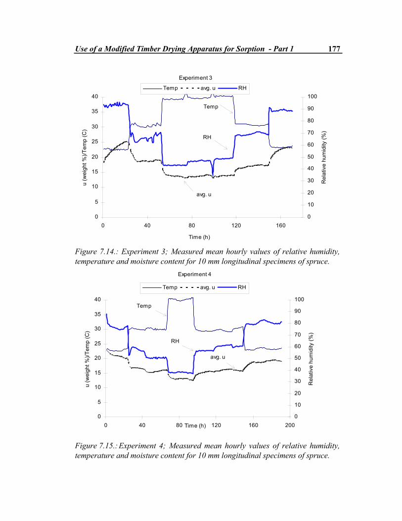
Use of a Modified Timber Drying Apparatus for Sorption - Part 1 177
Experiment 3
0
5
10
15
20
25
30
35
40
0 40 80 120 160
Time (h)
u (w
eigh
t %)/T
emp
(C)
0
10
20
30
40
50
60
70
80
90
100
Rel
ativ
e hu
mid
ity (%
)
Temp avg. u RH
avg. u
Temp
RH
Figure 7.14.: Experiment 3; Measured mean hourly values of relative humidity, temperature and moisture content for 10 mm longitudinal specimens of spruce.
Experiment 4
0
5
10
15
20
25
30
35
40
0 40 80 120 160 200Time (h)
u (w
eigh
t %)/T
emp
(C)
0
10
20
30
40
50
60
70
80
90
100
Rel
ativ
e hu
mid
ity (%
)
Temp avg. u RH
Temp
RH
avg. u
Figure 7.15.: Experiment 4; Measured mean hourly values of relative humidity, temperature and moisture content for 10 mm longitudinal specimens of spruce.

178 Chapter 7
One assumption could be that the calculated relative humidity was too low. But no moisture could have been added to the air, and only condensation could have changed the moisture conditions in the area between the measured wet-bulb (here the same as the saturation temperature) and the dry-bulb temperature. Such a change should have resulted in a lower relative humidity. Unless, however, there has been water at the bottom of the test section which has been absorbed by the air and made relative humidity increase. This could explain the high moisture contents for the low relative humidities. (Calculations with an assumption of higher relative humidity levels have been performed in Chapter 8). The moisture contents obtained from all these 4 experiments seem high compared to the final moisture content obtained in the initial drying experiment. This is the case even though the sets of specimens used in the 4 experiments had a longitudinal transport direction and the initial drying experiment had a set of specimens with a radial transport direction.
� �� �� �� �� �� �� �� �� �� ���
��
��
��
��
��
��
��
��
��
��
��
�
�
�
�
�
�� !
�"
#��$
%
&' $%
(�� "������
�)()���*
�)()���*
�)()���*
�)()���*
�)()���*
�)()���*
Figure 7.16.: Desorption «equilibrium» moisture content for specimens in experiment 2 (2,D,...)(drying from saturation) and experiment 4 (4,D,..) (approximately 2 weeks later). The specimens have been exposed to the climatic conditions in experiment 3 in between.(D=in desorption) Full sorption isotherms are measured sorption isotherms for spruce (Picea abies) grown in Scandinavia.

Use of a Modified Timber Drying Apparatus for Sorption - Part 1 179
From these results it seems as if the cyclic changes in climatic conditions (which the specimens in experiment 1 to 4 were exposed to) seem to decrease the total drying rate compared to the drying rate in the initial drying experiment with steady state conditions. In Chapter 5 is reported results from experiments in which parallel specimens have been exposed to step changes in relative humidity while the temperature has been held constant. For weekly step changes between 75% and 54% relative humidity, some specimens were soaked in water for the first week, while the others were exposed to 75% relative humidity. The sorption pattern in Chapter 5, figure 5.11 is characteristic for the sorption of all specimens independent of thickness and transport direction. (Both transversal, longitudinal, 5, 10 and 15 mm specimens were soaked). As can be seen from the figure, nearly the same moisture content is achieved for both the wetted and the dry specimens in desorption while there is a significant difference in absorption. The set of specimens in the initial drying experiment was dried for approximately one week and reached a rather low equilibrium level. The curve for the soaked specimens in figure 5.11 also reaches nearly the same desorption moisture content as the drier specimens, but there is a difference for absorption. The difference in absorption decreases from one cycle to another. This effect cannot be seen for desorption; however, the difference in desorption is already rather small after one week. 7.4 Concluding discussion When using the Small Drying Chamber (SDC), it turned out to be quite difficult to control the temperatures accurately. The room- and the outdoor temperature seem to affect the set temperatures considerably. The temperatures are set on an analogue scale, something which makes relatively small temperature changes hard to obtain. There also seems to be a potential problem with condensation in the apparatus, which is hard to control when running the apparatus. Thermal guards on the endplates and/or a vertical orientation for the test chamber may address this problem. A cooling system was added to the apparatus to make it possible to obtain lower temperatures than ambient in the test section. Because a significant amount of heat developed in the apparatus, the extra cooling had to be used to keep the temperature around ambient.
180 Chapter 7
The number of ancillary items (e.g., a compressor, several valves, pumps and cooling and heating units) makes the timber drying apparatus quite vulnerable to break down. The reliability of the load cell is uncertain and frequent calibration has been necessary. Because of the number of ancillary items, problems in keeping the temperature stable over long periods of time and drift in the weight measurement unit, the author does not find the apparatus appropriate for relatively long-lasting experiments (more than a couple of days). If a reliable relative humidity sensor had been placed in the test section the uncertainty of the moisture conditions in the small drying chamber might have been determined, and it would have been easier to evaluate the performance of the load cell. As it is today, there are two very important uncertain factors, the accuracy of the load cell and the control of the relative humidity. Because of these uncertainties, the reported data only reveal trends, not accurate responses to changes in environmental conditions. «The initial drying» experiment showed that the fast drying period for radial transport had finished after approximately 3.5 days for a 10-mm thick specimen of spruce, when the surrounding temperature was 20°C and the relative humidity approximately 85%. A rather low moisture content was obtained after 6.5 days compared to the general sorption isotherms for spruce. This might indicate that the relative humidity in the test section is actually lower than assumed or that there is a rather big internal difference between different specimens of spruce. The first assumption is believed to be the more likely. The four sorption experiments where the specimens have been exposed to both differences in relative humidity and temperature, result in rather high apparent «equilibrium» moisture contents, especially for the higher temperatures, 30°C and 40°C. Repeated experiments (exp.3 and 4 are repetitions of 1 and 2) show a small decrease in moisture content. It seems likely that the relative humidity in the chamber is higher than what has been calculated. A two-stage sorption process is observed in both absorption and desorption. A relatively larger part of the change in moisture content is found in the first steep part for desorption than in absorption. For all step changes, an «apparent» new equilibrium seem to have been reached within less than 2 days for all conditions (temperature and relative humidity).
Use of a Modified Timber Drying Apparatus for Sorption - Part 1 181
It may be that water forms or break away from molecule clusters at the surface (a fast process) before being sorbed or desorbed from available sites in the cell wall (a slow process). The process may also be related to the theory of physical ageing (Struik 1978); in which molecular destabilisation takes place in polymers, a breaking of hydrogen bonds, which is then followed by a slow asymptotic return to equilibrium.

182 Chapter 7

Use of a Modified Timber Drying Apparatus for Sorption - Part 2 183
Chapter 8
Use of a Modified Timber Drying Apparatus for Sorption in Spruce Part 2 - Calculations This chapter presents some comparative calculations for the results from the experiments presented in Chapter 7. The numerical moisture transport model described in Chapter 6 has been used for the calculations.
8.1 Introduction A simple Fickian way of modelling moisture transport in wood has not been found accurate enough for certain long-lasting sorption experiments. This kind of sorption measurements normally last for very long (normally a matter of months) and the slow sorption in the cell wall is observed. For wood in buildings this kind
184 Chapter 8
of climate exposure is rather rare. The environmental conditions on buildings and building components are changing all the time. For this reason cyclic measurements have been performed and a Fickian diffusion model has been used to evaluate whether this approach is suitable for moisture behaviour of wood in buildings, exposed to more rapid changes in surrounding climate. A systematic approach has been used to evaluate the importance of the different input parameters. For the calculations in this chapter hysteresis has not been considered. There are two reasons for this; 1) the model for hysteresis was not included in the numerical model at the time when these calculations were performed and 2) that the measured moisture contents are situated outside the data envelope for measured sorption isotherms for Scandinavian spruce. An investigation of the effect of a possible condensation in the timber drying apparatus has been done by the aid of calculations.
8.2 Comparison between experimental results and calculations
8.2.1 Description of simulation cases Three different cases of simulations have been done, here called Case A, Case B and Case C. Case A In Case A preliminary calculations to compare the overall consistency between the measurements described as experiment 1 to 4 (see Chapter 7) and calculations were done. These results are presented in figure 8.1 to 8.4. The input values used in the calculations are presented in table 8.1. An extreme sorption isotherm (Ahlgren 1972) has been used. The moisture contents obtained in the experiments are rather high and an extreme desorption isotherm was selected. The selected density is the density of the material used in the experiment, a rather low density compared to an average density for wood. The convective mass transfer coefficient (hp) is selected from Wadsø (1993). Most convective mass-transfer coefficients measured for wood is in the order of 30⋅10-9 kg⋅m-2s-1Pa-1. The thermal properties, except for the thermal moisture
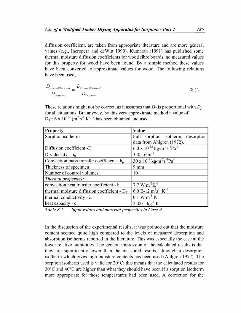
Use of a Modified Timber Drying Apparatus for Sorption - Part 2 185
diffusion coefficient, are taken from appropriate literature and are more general values (e.g., Incropera and deWitt 1990). Kumaran (1991) has published some thermal moisture diffusion coefficients for wood fibre boards, no measured values for this property for wood have been found. By a simple method these values have been converted to approximate values for wood. The following relations have been used; D
DD
Dp woodfibreboard
p spruce
T woodfibreboard
T spruce
−
−
−
−
≈ (8.1)
These relations might not be correct, as it assumes that DT is proportional with Dp for all situations. But anyway, by this very approximate method a value of DT= 6 x 10-12 (m2 s-1 K-1 ) has been obtained and used. Property Value Sorption isotherm Full sorption isotherm, desorption
data from Ahlgren (1972). Diffusion coefficient -Dp 6.0 x 10⁻¹² kg⋅m-1s-1Pa-1 Dry density - ρ0 350 kg⋅m-3 Convection mass transfer coefficient - hp 30 x 10-9 kg⋅m-2s-1Pa-1 Thickness of specimen 9 mm Number of control volumes 10 Thermal properties: convection heat transfer coefficient - h 7.7 W⋅m-2K-1 thermal moisture diffusion coefficient - DT 6.0 E-12 m2s-1 K-1 thermal conductivity - λ 0.1 W⋅m-1 K-1 heat capacity - c 2500 J⋅kg-1 K-1 Table 8.1 Input values and material properties in Case A In the discussion of the experimental results, it was pointed out that the moisture content seemed quite high compared to the levels of measured desorption and absorption isotherms reported in the literature. This was especially the case at the lower relative humidities. The general impression of the calculated results is that they are significantly lower than the measured results, although a desorption isotherm which gives high moisture contents has been used (Ahlgren 1972). The sorption isotherm used is valid for 20°C; this means that the calculated results for 30°C and 40°C are higher than what they should have been if a sorption isotherm more appropriate for those temperatures had been used. A correction for the
186 Chapter 8
temperature has not been done. However, this would have given a greater deviation. The calculated thermal moisture diffusion transport has no effect on the moisture sorption. Since there is no permanent temperature gradient across the specimen, it reaches a new thermal steady state situation rather quickly. Because of this the thermal moisture-diffusion coefficient has been set equal to zero in the following cases. As expected, there is no conformity between the measured results and the calculations for the first 2 to 3 days for experiment 1 and 2, figure 8.1 and 8.2. This is because the numerical model does not include liquid transport. Although the calculated results are significantly lower than the measured results the shape of the modelled and the measured moisture sorption curves are in good conformity for all conditions. This can indicate that the shape of the sorption isotherm is correct, but the level is not in accordance with the measurements. The agreement can also be an indication on an appropriate choice of mass-transfer coefficient and diffusion coefficient . Case A- Modified RH-levels Assume that the actual humidity level in the test section has been higher than evaluated from the temperature measurements (see Chapter 7). A coarse estimate has been done, and an extra humidity of 0.004 kg⋅kg-1 has been added to the humidity level in the test section for all the experiments. (This corresponds to an amount of condensate of approximately 1 litre per experiment). Calculations have been done for these humidity levels and presented in figure 8.1 to 8.4. The results show that there are relatively large differences in calculated and measured moisture content for the higher relative humidities (above approximately 70% RH) and the lower temperatures (near ambient). For temperatures near ambient and downwards a change in absolute humidity means more to the change in RH than for higher temperatures. Because of this only small differences can be seen between the two calculations, Case A and Case A-modified, for the higher temperatures and the lower relative humidities. (See a psychrometric chart for humid air at atmospheric pressure).

Use of a Modified Timber Drying Apparatus for Sorption - Part 2 187
0
5
10
15
20
25
30
35
40
0 20 40 60 80 100 120 140 160 180 200Time (h)
u (w
eigh
t %)/T
emp
(C)
0
10
20
30
40
50
60
70
80
90
100
Rel
ativ
e hu
mid
ity (%
)
Calculated
Calculated-mod. RH
Measured
Temp Original RH
Figure 8.1.: Experiment 1, Case A , A comparison between measured moisture contents and calculated results.
0
5
10
15
20
25
30
35
40
0 20 40 60 80 100 120 140 160 180 200 220 240Time (h)
u (w
eigh
t %)/T
emp
(C)
0
10
20
30
40
50
60
70
80
90
100
Rel
ativ
e hu
mid
ity (%
)
Calibration going on
Calculated
Calculated-mod.RH
Measured
Temp Original RH
Figure 8.2.: Experiment 2, Case A , A comparison between measured moisture contents and calculated results.

188 Chapter 8
0
5
10
15
20
25
30
35
40
0 20 40 60 80 100 120 140 160 180Time (h)
u (w
eigh
t %)/T
emp
(C)
0
10
20
30
40
50
60
70
80
90
100
Rel
ativ
e hu
mid
ity (%
)
Calculated Calculated mod. RH
Temp Original RH
Measured
Figure 8.3.: Experiment 3, Case A , A comparison between measured moisture contents and calculated results.
0
5
10
15
20
25
30
35
40
0 20 40 60 80 100 120 140 160 180 200Time (h)
u (w
eigh
t %)/T
emp
(C)
0
10
20
30
40
50
60
70
80
90
Rel
ativ
e hu
mid
ity (%
)
Calculated
Calculated mod. RH
Measured
Temp Original RH
Figure 8.4.: Experiment 4, Case A , A comparison between measured moisture contents and calculated results. There is an overall better agreement between measurements and the first calculations, Case A, for all humidity levels. The results of the calculations with
Use of a Modified Timber Drying Apparatus for Sorption - Part 2 189
the modified RH-levels show rather significant differences between measured and calculated moisture content from one temperature and RH-level to another. This means that if there has been any condensation it has probably not occurred at the same rate throughout the whole experiments. It also seems as if a rather significant addition in absolute humidity for higher temperatures and lower relative humidities has relatively little effect on the calculated moisture contents. Case B To evaluate the influence of the different material properties a design matrix with 3 different material properties has been set up. See table 8.2 for the selected properties and their values. The linear function for the diffusion coefficient is described in Chapter 6. All together 8 simulations for experiment 3 and 4 have been performed. Some of the results from these calculations are presented in figure 8.5 and 8.6. The level of the full sorption isotherm and the simplified two-step linear model are very much the same especially above 50 % RH. The calculated results show very little difference between these two kinds of sorption isotherms. Therefore only the results where the full sorption isotherm has been used, have been presented here. Since the moisture capacity is the derivative of the sorption isotherm, this means that the moisture capacity is also varying with the relative humidity. For the two-step linear sorption isotherm the moisture capacity is constant for 2 intervals, one for relative humidities up to 70 % and one for the humidities above. The situations where the diffusion coefficient has been kept constant (6 x 10-12 kgm-1s-1 Pa-1 ) and only the density has been varied (B1, B3, B5 and B7) show that the sample with the lower density (350 kg⋅m-3) has a faster sorption and reaches an «equilibrium» level faster than the corresponding case with a higher density (500 kg⋅m-3). The lower-density case is also more in accordance with the experimental results, something which is expected since the density of the specimens is very close to 350 kg⋅m-3. For higher relative humidities, the calculated results for the cases with different levels of diffusion coefficients differ to a relatively great extent. In the area of 80 - 90 % relative humidity the value of the linear increasing diffusion coefficient is
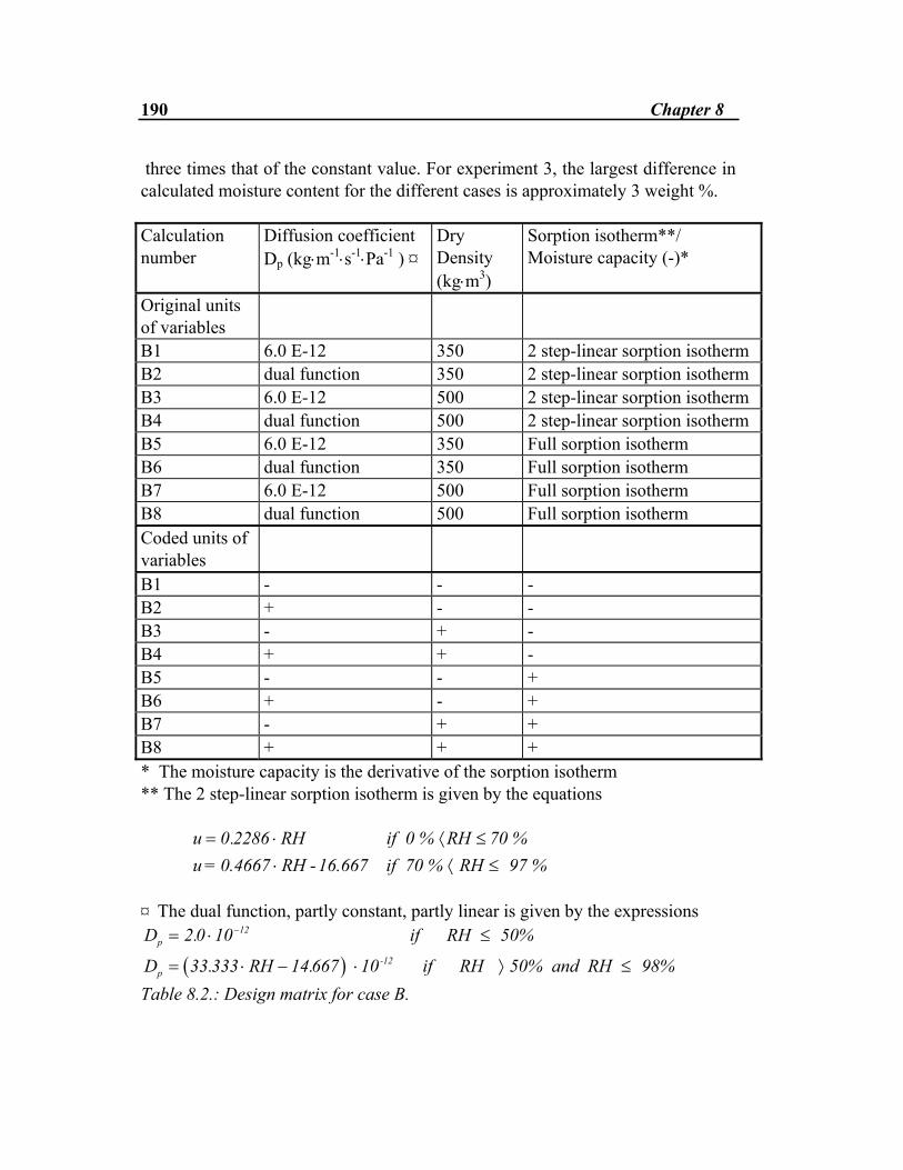
190 Chapter 8
three times that of the constant value. For experiment 3, the largest difference in calculated moisture content for the different cases is approximately 3 weight %. Calculation number
Diffusion coefficient Dp (kg⋅m-1⋅s-1⋅Pa-1 ) ¤
Dry Density (kg⋅m3)
Sorption isotherm**/ Moisture capacity (-)*
Original units of variables
B1 6.0 E-12 350 2 step-linear sorption isotherm B2 dual function 350 2 step-linear sorption isotherm B3 6.0 E-12 500 2 step-linear sorption isotherm B4 dual function 500 2 step-linear sorption isotherm B5 6.0 E-12 350 Full sorption isotherm B6 dual function 350 Full sorption isotherm B7 6.0 E-12 500 Full sorption isotherm B8 dual function 500 Full sorption isotherm Coded units of variables
B1 - - - B2 + - - B3 - + - B4 + + - B5 - - + B6 + - + B7 - + + B8 + + + * The moisture capacity is the derivative of the sorption isotherm ** The 2 step-linear sorption isotherm is given by the equations
u RH = ⋅ ⟨ ≤
⋅ ⟨ ≤0 2286. if 0 % RH 70 %
u = 0.4667 RH -16.667 if 70 % RH 97 %
¤ The dual function, partly constant, partly linear is given by the expressions
( )D
D RHp = ⋅ ≤
= ⋅ − ⋅ ⟩ ≤
−2 0 10
33 333 14 667
12.
. .
if RH 50%
10 if RH 50% and RH 98%p-12
Table 8.2.: Design matrix for case B.
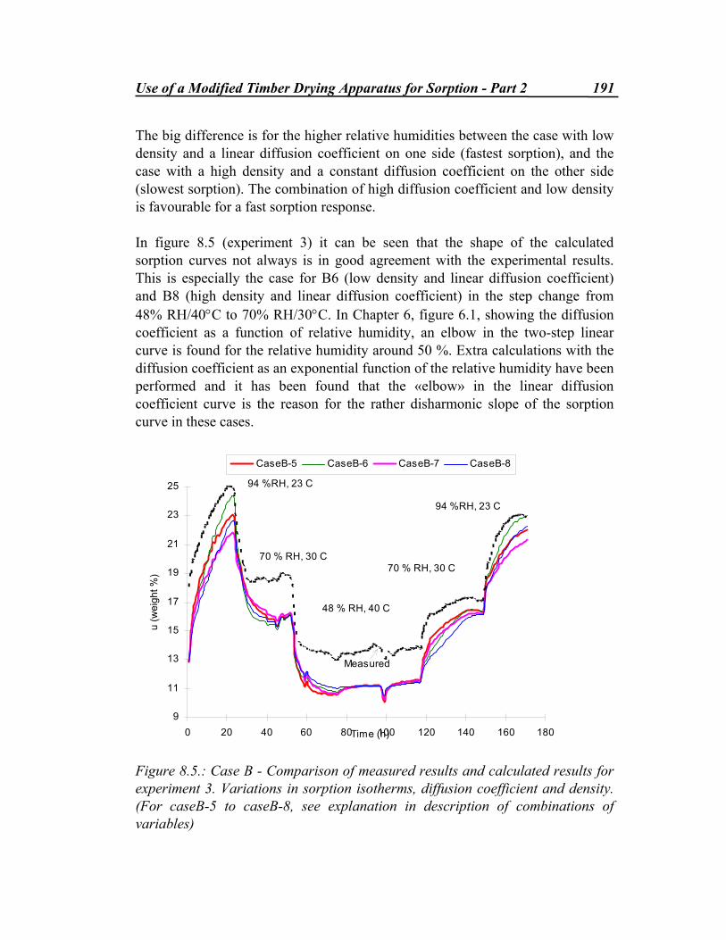
Use of a Modified Timber Drying Apparatus for Sorption - Part 2 191
The big difference is for the higher relative humidities between the case with low density and a linear diffusion coefficient on one side (fastest sorption), and the case with a high density and a constant diffusion coefficient on the other side (slowest sorption). The combination of high diffusion coefficient and low density is favourable for a fast sorption response. In figure 8.5 (experiment 3) it can be seen that the shape of the calculated sorption curves not always is in good agreement with the experimental results. This is especially the case for B6 (low density and linear diffusion coefficient) and B8 (high density and linear diffusion coefficient) in the step change from 48% RH/40°C to 70% RH/30°C. In Chapter 6, figure 6.1, showing the diffusion coefficient as a function of relative humidity, an elbow in the two-step linear curve is found for the relative humidity around 50 %. Extra calculations with the diffusion coefficient as an exponential function of the relative humidity have been performed and it has been found that the «elbow» in the linear diffusion coefficient curve is the reason for the rather disharmonic slope of the sorption curve in these cases.
9
11
13
15
17
19
21
23
25
0 20 40 60 80 100 120 140 160 180Time (h)
u (w
eigh
t %)
CaseB-5 CaseB-6 CaseB-7 CaseB-8
48 % RH, 40 C
70 % RH, 30 C
94 %RH, 23 C
94 %RH, 23 C
70 % RH, 30 C
Measured
Figure 8.5.: Case B - Comparison of measured results and calculated results for experiment 3. Variations in sorption isotherms, diffusion coefficient and density. (For caseB-5 to caseB-8, see explanation in description of combinations of variables)

192 Chapter 8
The other distinct cases are B5 (low density and constant diffusion coefficient) and B7 (high density and constant diffusion coefficient) in the step change from 70% RH/30°C to 94% RH/23°C for experiment 3 (figure 8.5). For these cases a constant diffusion coefficient for all humidity regions has been used. A higher diffusion coefficient gives a better correspondence with the measured results in the higher relative humidity region. For some of the environmental conditions there is a complete difference in the shape of the calculated moisture content and the measured moisture content, e.g., for experiment 4 ( figure 8.6) at the end of the «desorption level» of 55% RH and 30°C and for the «absorption level» of 70% RH and 23°C. This might indicate that the assumed relative humidity is different from the actual relative humidity in the test section.
9
11
13
15
17
19
21
23
25
0 20 40 60 80 100 120 140 160 180 200Time (h)
u (w
eigh
t %)
CaseB-5 CaseB-6 CaseB-7 CaseB-8
70 % RH, 23 C
55 % RH, 30 C
38 % RH, 40 C
70 % RH, 23 C
55 % RH, 30 C
Measured
Figure 8.6.: Case B - Comparison of measured results and calculated results for experiment 4. Variations in sorption isotherms, diffusion coefficient and density. (For caseB-5 to caseB-8, see explanation in description of combinations of variables). Case C

Use of a Modified Timber Drying Apparatus for Sorption - Part 2 193
The influence of variations of the convective mass-transfer coefficient has not yet been studied. From the experience with case B, a case C was set up with a full sorption isotherm and variations of the convective mass-transfer coefficient, the diffusion coefficient and the dry density. The reason for the selected levels of material properties is given in previous chapters. The selection of the high level hp (hp = 100 ⋅10-9 kg⋅m-2s-1 Pa-1) however, has not yet been explained. The value is selected from data presented in Wadsø (1993), page 61. A mass transfer coefficient of 100⋅10-9 kg⋅m-2s-1⋅Pa-1 is a fairly high value for sorption experiments with an air velocity of 0.1 to 0.3 m⋅s-1 and a length of the specimen like 0.07 m. The calculations performed and the input parameters are shown in table 8.3. Calculation number Diffusion
coefficient* Dp (kg⋅m-1s-1Pa-1)
Dry Density ρ0
(kg⋅m-3) Convection mass transfer coefficient hp (kg⋅m-2s-1 Pa-1)
Original units of variables C1 6.0 E-12 350 30 E-9 C2 exponential function 350 30 E-9 C3 6.0 E-12 500 30 E-9 C4 exponential function 500 30 E-9 C5 6.0 E-12 350 100 E -9 C6 exponential function 350 100 E -9 C7 6.0 E-12 500 100 E -9 C8 exponential function 500 100 E -9 Coded units of variables C1 - - - C2 + - - C3 - + - C4 + + - C5 - - + C6 + - + C7 - + + C8 + + + *The exponential function for diffusion coefficient is described in Chapter 6 Table 8.3.: Design matrix for caseC. Some results from these calculations are compared with the measured results for experiment 3 and 4 in figure 8.7 and 8.8.
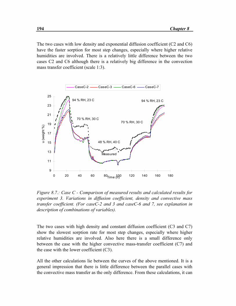
194 Chapter 8
The two cases with low density and exponential diffusion coefficient (C2 and C6) have the faster sorption for most step changes, especially where higher relative humidities are involved. There is a relatively little difference between the two cases C2 and C6 although there is a relatively big difference in the convection mass transfer coefficient (scale 1:3).
9
11
13
15
17
19
21
23
25
0 20 40 60 80 100 120 140 160 180Time (h)
u (w
eigh
t %)
CaseC-2 CaseC-3 CaseC-6 CaseC-7
94 % RH, 23 C
70 % RH, 30 C
48 % RH, 40 C
70 % RH, 30 C
94 % RH, 23 C
Measured
Figure 8.7.: Case C - Comparison of measured results and calculated results for experiment 3. Variations in diffusion coefficient, density and convective mass transfer coefficient. (For caseC-2 and 3 and caseC-6 and 7, see explanation in description of combinations of variables). The two cases with high density and constant diffusion coefficient (C3 and C7) show the slowest sorption rate for most step changes, especially where higher relative humidities are involved. Also here there is a small difference only between the case with the higher convective mass-transfer coefficient (C7) and the case with the lower coefficient (C3). All the other calculations lie between the curves of the above mentioned. It is a general impression that there is little difference between the parallel cases with the convective mass transfer as the only difference. From these calculations, it can
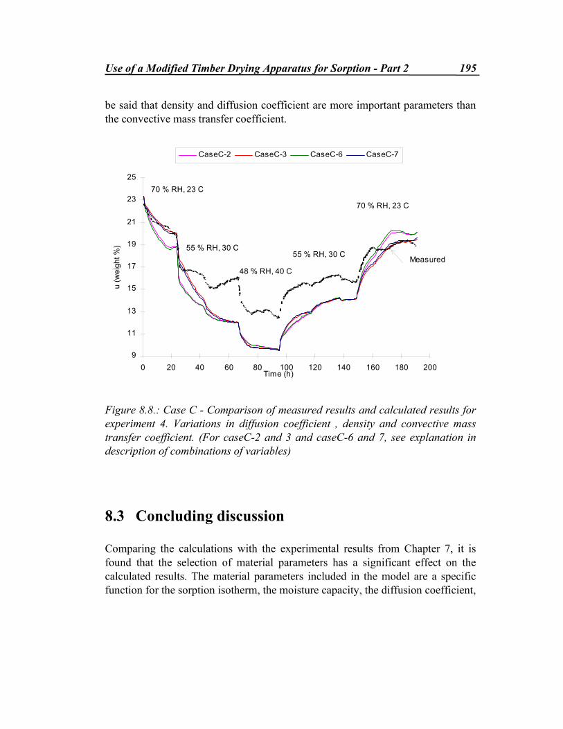
Use of a Modified Timber Drying Apparatus for Sorption - Part 2 195
be said that density and diffusion coefficient are more important parameters than the convective mass transfer coefficient.
9
11
13
15
17
19
21
23
25
0 20 40 60 80 100 120 140 160 180 200Time (h)
u (w
eigh
t %)
CaseC-2 CaseC-3 CaseC-6 CaseC-7
70 % RH, 23 C
55 % RH, 30 C
48 % RH, 40 C
70 % RH, 23 C
55 % RH, 30 CMeasured
Figure 8.8.: Case C - Comparison of measured results and calculated results for experiment 4. Variations in diffusion coefficient , density and convective mass transfer coefficient. (For caseC-2 and 3 and caseC-6 and 7, see explanation in description of combinations of variables)
8.3 Concluding discussion Comparing the calculations with the experimental results from Chapter 7, it is found that the selection of material parameters has a significant effect on the calculated results. The material parameters included in the model are a specific function for the sorption isotherm, the moisture capacity, the diffusion coefficient,

196 Chapter 8
a density value, a convective mass-transfer coefficient and some thermal properties. The climatic parameters used are measured values on hourly basis for relative humidity and temperature. As the driving potential for the model is vapour pressure, the relative humidity and the temperature are recalculated to a vapour pressure. The calculations performed have been divided into 3 cases (Case A, B and C). Case A is a preliminary calculation to compare the overall consistency between the measurements described in Chapter 7 and the described model. The results from the preliminary calculations showed that the assumed level of the sorption isotherm is very important for determining the level of the calculated curve of moisture content versus time. The sorption isotherm used in case A is a desorption isotherm (Ahlgren 1972), showing fairly high equilibrium moisture contents. As shown previously in this thesis, measured sorption isotherms on spruce (Picea abies) in Scandinavia show rather big differences in moisture content. The difference in moisture content from the «lowest» absorption isotherm to the «highest» desorption isotherm for the same relative humidity is between 3 - 7 weight %. Since the measured moisture contents were rather high, a «high» sorption isotherm was selected for the calculations. As the calculated relative humidities from the measurements have been found uncertain some calculations have been done with modified RH-levels. No better agreement between measurements and calculations were found. For case B and case C a systematic approach has been used to look closer into the effect of combinations of material parameters. Two different values for three different material parameters have been combined, so that each case consists of eight calculations for each experiment with eight different combinations of the actual material parameters. In case B, one of the factors studied was a linearisation of the sorption isotherm. A two-step linearisation was fitted to the full sorption isotherm. The calculations showed very little difference in moisture content between a full sorption isotherm and a well-fitted, two-step linearisation. The choice of the two other variable parameters in case B, namely basic wood density (dry) and diffusion coefficient, Dp, showed a significant effect on the sorption rate. The overall impression of case B is that the calculation with a density of 350 kg⋅m-3 and a two-step linear diffusion coefficient gives the best fit. Diffusion coefficient measurements reported in Chapter 4 show that the diffusion
Use of a Modified Timber Drying Apparatus for Sorption - Part 2 197
coefficient is dependent on relative humidity. The density of the test specimens is approximately 350 kg⋅m-3 . For case C a full sorption isotherm was used and variations of the convective mass-transfer was introduced in addition to diffusion coefficient and density. The selected values for the convective mass-transfer coefficient were selected from results in a thorough study of convective mass-transfer coefficients for wood given by Wadsø (1993). A lower level value of hp =30 kg⋅m-2s-1 Pa-1 and a higher level value of hp =100 kg⋅m-2s-1 Pa-1 were selected. The results from case C showed that calculations with a mass-transfer coefficient as the only difference varied very little. Complementary calculations with an even higher value (hp = 200 kg⋅m-2s-1 Pa-1) of the coefficient did not make any significant differences to the result. The diffusion coefficient for case C was either a constant value or an exponential function of relative humidity. The wood density values were the same as for case B, 350 kg⋅m-3 and 500 kg⋅m-3. These calculations confirm the overall impression from case B that the density and the diffusion coefficient as a function of relative humidity are the most important parameters, in addition to the level of the sorption isotherm. The model includes a part where moisture transport is considered due to a thermal gradient. For the measurements reported in Chapter 7, the thermal gradient is active only in the step changes which took place at most for half an hour. Because of this, moisture transport due to a thermal gradient has no effect in this work. The temperature dependence of the diffusion coefficient has not been considered. A search in literature gave no unambiguous answer to if a significant dependency exists. The temperature dependence of the sorption isotherm has also been neglected. The variations for the reported isotherms for spruce are fairly large, larger than any effect of temperature. If a temperature variation of the sorption isotherm had been included, the discrepancies between the measured and the calculated values for the higher temperature levels would have been even larger. As a first approach to modelling the sorption of wood exposed to cyclic environmental changes, the model has proved to be rather promising. The shape of the measured and the calculated curves corresponds very well, but the magnitude of the estimated moisture contents show significant differences. This is most likely due to the magnitude of the sorption isotherm used in the model.

198 Chapter 8

Chapter 9
Conclusions The main conclusions of this work and recommendations for further research are given in this chapter.
9.1 Main conclusions This thesis is a result of a comprehensive study on hygroscopic moisture transport in wood in general and spruce (Picea abies) in particular. Spruce together with pine are the main wooden building materials used in Norway. Wood and wooden materials in buildings are exposed to smaller or larger changes in climate continuously. Wood used at the exterior of a building is exposed to rather extreme diurnal and annual climatic cycles, while wood used indoor and within structures are exposed to less extreme, but nevertheless present changes. Uncertainties concerning transient wood-water relations in buildings and building components have demanded a more thorough investigation on basic moisture transport in wood and related properties.
200 Chapter 9
The work reported in this thesis can be divided into three main tasks. In the first task, the author has been concerned with studying the theories and the present knowledge of moisture sorption and moisture transport in wood. Material properties have also been measured and investigated in this task. It has been found that diffusion coefficients, Dp, determined from cup measurements are increasing with an increasing average relative humidity across a wooden specimen. It has also been confirmed that if diffusion coefficients, DC, determined from transient sorption measurements are to be converted to Dp,, significant variations in diffusion coefficients can be achieved depending on the parameters included in the conversion factor. Absorption and desorption isotherms of spruce (Picea abies) measured in this work have been compared with corresponding measurements on spruce performed in other Nordic countries, and significant deviations exist. In the second task of this thesis experimental investigations on wood exposed to cyclic step-changes in climatic conditions have been performed. Two different sets of experiments have been performed. In the main set of experiments (Chapter 5) an experimental apparatus has been designed and set up in the laboratory. Well known principles for measurements of moisture sorption in wood have been employed. As there is a demand for less labour intensive and more efficient methods for measuring moisture sorption in wood, another set of experiments has been conducted (Chapter 7). These experiments have been conducted in the laboratory at Department of Chemical and Process Engineering (CAPE), University of Canterbury, New Zealand. In these experiments, another more efficient principle of measurement, originally meant for drying experiments, has been employed and assessed for measuring moisture sorption in wood. The results from four different series with diurnal and weekly cycles between two different levels have been reported. A two-step sorption process has been observed with the major change in moisture content in the first fast initial part. No significant phase lag has been observed for neither transverse nor longitudinal specimens up to 10 mm thickness. A repetitive pattern in moisture content change is found for both weekly and daily changes. The same level of moisture content is reached in both absorption and desorption every cycle. Although average moisture contents have been measured only, the fast response in moisture sorption indicates that significant moisture gradients are present immediately after a relatively large change in surrounding humidity. The results from four different sorption experiments, conducted at CAPE, have indicated the presence of the same two-step sorption process, with the major
Conclusions 201
change in moisture content within the first initial part of sorption, lasting for at most two days for 10 mm specimens. The specimens in these experiments were exposed to time gradients in both temperature and relative humidity. The overall impression from these experiments is that the apparent «equilibrium» moisture contents are rather high for all temperature and humidity levels. The reason for this has not been possible to fully explain. However, weaknesses in the principle of measurement have been revealed. As it is today there are two very important uncertain factors, the accuracy of the load cell (weighing unit) and the control of the relative humidity (environmental conditions). For relatively long-lasting sorption measurements on wood, saturated salt-solutions have shown to give more stable environmental conditions than conditioned air obtained from a mixture of heated water and air. A better accuracy of the weight measurements is obtained by a scale of the Mettler type than by use of a load cell. In the third task of this thesis, a one-dimensional transient model for moisture transport in wood is set up. The model is based on Fick’s law with water vapour pressure and temperature as driving potentials. A model for hysteresis has been proposed and included in the model. Comparisons between the experimental results obtained in this work and calculations have been done. The level of the absorption and the desorption isotherm is the most important parameter in order to obtain good fit between measurements and calculations. A better agreement is found if hysteresis is taken into account, compared to calculations were only an average sorption isotherm is used. The repetitive moisture content situation is dependent on the immediate past history, i.e., whether the calculations start on the absorption or the desorption isotherm or in the hysteresis region. In calculations, it is also found that the diffusion coefficient and its dependency on RH and the density of the wood have a certain influence on the sorption rate. The convection mass transfer coefficient on the other side has very little influence on the average moisture content. As an approach to modelling moisture transport in wood exposed to cyclic environmental changes in the hygroscopic range, the model has proved promising. The shape of the measured and the calculated curves presented in this work correspond very well. This might imply that application of linear intermediate curves, based on empirical data, could be a suitable way of modelling hysteresis in wood.

202 Chapter 9
9.2 Recommendations for further work Not very much basic experimental work on wood exposed to cyclic climatic conditions has been done throughout the years. One reason for this is presumably the fact that it is a very time consuming work performing such experiments. Nevertheless, it is very important because the only way of achieving new knowledge is through systematic and careful experimental work. Numerical models do exist as helpful tools, but they are only helpful if good experimental data exist for the purpose of verification. It has been shown in this thesis that there is a considerable deviation in reported sorption isotherms for spruce (Picea abies) performed in Nordic countries. It is shown that the level of the absorption and desorption isotherm is the limiting factor in achieving a good fit in modelling moisture sorption in spruce exposed to relatively rapid changes in relative humidity. This implies that the sorption isotherms should be investigated more carefully. It has been stated earlier (Wadsø 1993) that the time to final equilibrium for wood exposed to constant surrounding conditions is very long, indeed. However, the experiments performed in this project have shown that an apparent equilibrium level is reached rather fast. The interpretation of time to equilibrium should obviously been given more careful thoughts. What are the differences in moisture content for specimens which have been exposed to the same climatic conditions for example 1 week, 1 month or 2 months respectively? Very careful absorption and desorption isotherm measurements on parallel specimens of wood should be performed simultaneously in different laboratories in order to compare the results and assess the facilities. The parallel specimens involved in such experiments should be carefully selected from different sites and different origins in order to find out what are the real variations between specimens to be expected. The measurements on small pieces of wood exposed to changing environmental conditions performed in this work have been limited to: • weekly and daily step changes between 54% and 75%, and 75% and 94%
relative humidity respectively, and a temperature fairly constant around 23°C. • 1-4 day step changes in both relative humidity and temperature. Relative
humidity varying from around 40% to 95% and temperature varying between 23 and 40°C.
Conclusions 203
It has been concluded that the Fickian model fits relatively well to the set of experimental data presented. But as the sets of data are quite limited, similar experiments, not necessarily with step changes, for different temperatures and different levels of relative humidities should be performed and compared with calculations. Only very few intermediate curves for wood do exist. It would be useful, through some more careful experiments, to try to map some kind of repetitive pattern for these curves. A thermal moisture diffusion coefficient, DT, has been applied in this work. Experimental work on moisture transport in wood as a result of a space gradient in temperature only, and as a result of space gradients in both relative humidity and in temperature should be performed. Such experiments could contribute to a further understanding of moisture transport in wood due to a thermal gradient.

204 Chapter 9
References Absetz, I., 1993, Sorption isotherm and moisture diffusivity comparison of spruce and pine, Seminarium I Trämekanik, Borås, Sweden, 28 – 29 October. Absetz, I., Koponen, S. and Lehtinen M., 1993, Effects of cell and cell wall structure on mechanical and moisture physical properties of wood, Annual report, Helsinki University of Technology, Laboratory of Structural Engineering and Building Physics. Absetz, I., Koponen, S., 1997, Fundamental diffusion behaviour of wood, International Conference of Cost Action E8 Wood Mechanics, Theme: Wood-Water Relations, Copenhagen , June 16 – 17. Advantech, 1993, Genie Data Acquisition and Control Software for Windows, American Advantech Corporation. Ahlgren, L., 1972, Fuktfixering i porösa byggnadsmaterial (Moisture fixation in porous building materials), Report 36, Division of Building Technology, The Lund Institute of Technology, Sweden, (in Swedish). Arfvidsson, J., 1994, Isoterma Fuktförlopp i porösa material-beräkning och utvärdering av mätdata. (Isothermal moisture transport in porous materials – calculations and assessment of experimental data) Rapport TVBH-1007, Avd. för Byggnadsfysik, Lunds Tekniska Högskola, (In Swedish). ASHRAE, 1989, Handbook of Fundamentals, American Society of Heating, Refrigerating and Air-conditioning Engineers, Atlanta, USA. Avramidis, S., 1997, The basics of sorption, International Conference of COST
206
Action E8, Mechanical Performance of Wood and Wood Products, Theme: Wood-Water Relations, Copenhagen, Denmark, June 16 -17. Avramidis, S., Englezos, P. and Papathanasiou, T., 1992, Dynamic nonisothermal transport in hygroscopic porous media: moisture diffusion in wood, AIChE Journal, Vol. 38, No.8, pp 1279-1287. Avramidis, S., Hatzikiriakos, S.G. and Siau, J.F., 1994, An irreversible thermodynamics model for unsteady-state nonisothermal moisture diffusion in wood, Wood Science and Technology, Vol. 28, pp. 349 - 358. Avramidis, S., Kuroda, N., Siau J.F., 1987, Experiments in nonisothermal diffusion of moisture in wood. Part II., Wood and Fibre Science, Vol. 19, Nr.4, pp 407 – 413. Avramidis, S., Siau, J.F., 1987, Experiments in nonisothermal diffusion of moisture in wood, Part 3, Wood Science and Technology, Vol. 21, pp 329 - 334. Bergheim, E., Geving, S., Time B., 1998, Measurements of water vapour permeability and sorption isotherms for various building materials, Norwegian Building Research Institute, Draft copy, Project report. Bertelsen, N.H., 1984a, Diffusionsmåling med Kopmetoden på Rødgran,(Cup measurements of water vapour permeability of spruce) Teknisk Rapport nr. 129/83, DTH, Department of Civil Engineering, Building Materials Laboratory, Veksø, Denmark, (In Danish). Bertelsen, N.H., 1984b, Fugttransport målt med kopmetoder. Nordtest workshop, bagrund og udviklingsområder. (Moisture transport measured with cup methods, Nordtest workshop, background and further development issues). Byggeteknik, Teknologisk Institut, Denmark, (In Danish). Biggerstaff, T., Drying Diffusion Coefficients in Wood as affected by temperature, Forest Products Journal, March, 1965, pp 127 - 133. Billmeyer, F.B.Jr., 1984, Textbook of Polymer Science, third Edition, A Wiley-Interscience Publication, John Wiley and Sons. Box, G.E.P., Hunter, W.G. and Hunter, J.S., 1978, Statistics for experimenters, An introduction to design, data analysis, and model building, John Wiley and Sons, Toronto.
References 207
Boye, C., 1986, Undersøgelse af rødgranveds damppermeabilitet (An investigation on vapour permeability of spruce), Træteknik, Teknologisk Institut, Danmark, (In Danish). Bramhall, G., 1976, Fick’s laws and bound-water diffusion, Wood Science, Vol. 8, No. 3, pp 153 - 161. Bramhall, G., 1979, Sorption diffusion in wood , Wood Science, Vol. 12, No. 1, pp 3 - 13. Burch, D., 1997, Mechanical Engineer at National Institute of Standards and Technology, USA, Personal communication. Burch, D.M., Thomas, W.C. and Fanney, A.H., 1992, Water vapor permeability measurements of common building materials, BA-92-6-2, ASHRAE Transactions V.98.Pt.2. Carrington, M., 1996, High-temperature seasoning of softwood boards, determination of mechanical properties at evaluated temperatures, Mc.S Thesis, CAPE, University of Canterbury, New Zealand. CEN, 1995, Building materials - determination of moisture content by drying at elevated temperature, Draft of European Standard, pr EN xxx, CEN/TC 89, N338 E rev. 1995-01-26. Chomcharn A., Skaar, C., 1983, Dynamic sorption and hygroexpansion of wood wafers exposed to sinusoidally varying humidity, Wood Science and Technology, Vol. 17, pp 259 - 277. Choong, E.T. and Fogg, P.J., 1968, Moisture movement in six wood species, Forest Products Journal, Vol.18, No.5, pp 66 - 70. Choong, E.T., 1963, Movement of moisture through a softwood in the hygroscopic Range, Forest Products Journal, Vol. 13, pp 489 - 498. Christensen, G.N., 1965, The rate of sorption of water vapor by thin materals, Division of Forestr Products, Commonwealth Scientific and Industrial Research Organization, Australia. Cohan, L.H., 1944, Hysteresis and the capillary theory of adsorption of vapors, Journal of the American Chemical Society, Vol. 66, pp 98 - 105.
208
Comstock, G.L., 1963, Moisture diffusion coefficients in wood as calculated from adsorption, desorption and steady state data, Forest Products Journal, Vol. 13 (March), pp 96 - 103. Crank, J., 1975, The mathematics of diffusion. Oxford Science Publications. Second Edition. Clarendon Press, Oxford. Cunningham, M.J., 1994, A Model to Explain «Anomalous» Moisture Sorption in Wood Under Step Function Driving Forces, Building Research Association of New Zealand. Cunningham, M.J., 1990, Modelling of moisture transfer in structures-II. A comparison of a numerical model, an analytical model and some experimental results. Building and Environment, Vol.25, No.2, pp. 85-94. Cunningham, M.J., 1992, Moisture Diffusion due to Periodic Moisture and Temperature Boundary Conditions-an Approximate Steady Analytical Solution with Non-Constant Diffusion Coefficients. Building and Environment, Vol.27, No.3, pp. 379-386. Dakin, Mark C., 1996, Design of a timber drying apparatus, a Project Report submitted for the Bachelor of Engineering (Chemical and Process), University of Canterbury, New Zealand, October. Danvak, 1987, Danvak, Varme- og Klimateknik Grundbog (Handbook in heat and air condition), Teknisk forlag A/S København, Redaktion: Hansen, H.E m.fl., (In Danish). Dent, R.W., 1977, A multilayer theory for gas sorption, Part I: Sorption of a single gas, Textile Research Journal, Vol. 47, pp 145-152. Droin, A., Taverdet, J.L., Vergnaud, J.M., 1988, Modeling the kinetics of moisture adsorption by wood, Wood Science and Technology, Vol. 22, pp 11-20. Droin-Josserand, A. Taverdet, J.L., Vergnaud, J.M., 1988, Modelling the absorption of moisture by wood in an atmosphere of constant and programmed relative humidity, Wood Science and Technology, Vol. 22, pp 299 – 310.
References 209
Earl, W., 1996, Senior Technician at Department of Chemical and Process Engineering, University of Canterbury, New Zealand, Personal communication. Geving, S., Thue, J.V., 1996, Measurements and computer simulations of the hygrothermal performance of leightweight roofs. In: Proceedings of the 4th Symposium on Building Physics in the Nordic Countries, Espoo, Finland, September 9. - 10. Hailwood, A.J., Horrobin, S., 1946, Absorption of water by polymers: Analysis in terms of a simple model, Trans. Faraday Soc. 42B, pp 84 -102. Hansen, K. K, 1986, Sorption isotherms, A Catalogue, Technical Report 162/86, Building Materials Laboratory, The Technical University of Denmark. Hedlin, C.P., 1967, Sorption isotherms of twelve woods at subfreezing temperatures. Forest Products Journal , Vol. 17, No. 12, pp 43 - 48. Hens, H., 1996, Modelling. Final Report Task 1., International Energy Agency, Energy Conservation in Building and Community Systems, Annex 24 Heat, Air and Moisture Transport in New and Retrofitted Building Envelope Parts (HAMTIE). Laboratorium Bouwfysica, K.U.-Leuven, Belgium. Hjort, S., 1991, How to keep coated wood structures sufficiently dry to avoid damage caused by rot. In Proc. IRG/WP (International Research Group on Wood Preservation) May 1991 in Kyoto, Japan (IRG/WP/2376). Homb, A., Skogstad, H.B., Thue, J.V., 1993, Laboratory measurements of moisture conditions in different wood frame walls, Third Symposium on Building Physics in the Nordic Countries, Copenhagen, 13 - 15. September 1993. Håkansson, H., 1994, Experimentella studier av transient sorption i cellväggen i trä (Experimental investigations of transient sorption in the cell wall of wood), Rapport TABK-94/3021, Lunds Universitet, Lunds Tekniska Högskola, Institutionen för byggnadskonstruktionslära, (In Swedish). Håkansson, H., 1995a, Experimentella studier av transient sorption i cellväggen i trä, Del II-fortsatta mätningar, (Experimental investigations of transient sorption in the cell wall of wood, Part II) Rapport TABK-95/3030, Lunds Universitet, Lunds Tekniska Högskola, Institutionen för byggnadskonstruktionslära, (In Swedish).
210
Håkansson, H., 1995b, A non-linear model for time-dependent moisture sorption in wood, Rapport TABK-95/3031, Lund University, Lund Institute of Technology, Department of Building Science. Incropera, F.P., De Witt, D.P., 1990, Fundamentals of heat and mass transfer, Third Edition, John Wiley and Sons. Jaafar, F., Michalowski, S., 1990, Modified BET equation for sorption/desorption isotherms, Drying Technology, Technical Note, Vol. 8, No. 4, pp 811 - 827. Joy, F.A., Wilson, A.G., 1965, Standardization of the dish method for measuring water vapour transmisson , Humidity and Moisture, Principles and Methods of Measuring Moisture in Liquids and Solids, Volume 4, No. 31, pp 259 - 270, (International Symposium on Humidity and Moisture, 1963). Kaminski, W., Kudra, T., 1996, Material-Moisture Equilibrium - Lecture Notes, Faculty of Process and Environmental Engineering, Technical University of Lodz, Poland. Kawai, S., Nakato, K. and Sadoh, T., 1978, Prediction of moisture distribution in wood during drying, Mokuzai Gakkaishi, Vol. 24, No.8, pp 520-525, 1978. Kawai, S., Nakato, K., Sadoh, T., 1980, Moisture movement in wood in the hygroscopic range, Memoirs of the College of Agriculture, Kyoto University, No. 115, pp. 1-32. Keey, R.B, 1978, Introduction to industrial drying operations, Pergamon Press, Oxford. Keey, R.B., 1997, Professor Emeritus at Department of Chemical and Process Engineering, University of Canterbury, New Zealand, Personal communication. Kelly, M.W., Hart, A.C., 1970, Water vapour sorption rates by wood cell walls, Wood and Fiber, Vol. 1, No.4 pp 270 - 283. Kollmann, F.F.P., 1961, High temperature drying, research, application, and experience in Germany, Forest Products Journal, November, pp 508-515 . Kollmann, F.F.P., Côté, W.A.Jr., 1968, Principles of wood science and technology, I: Solid wood, Springer Verlag, Berlin-Heidelberg-New York.
References 211
Koponen, H., 1986, Transport processes in Finnish birch, pine and spruce. Part I. Sorption isotherms and moisture diffusion coefficients, Papper och Traa Nr. 6-7, Volume 68, pp 465 - 474, Coden: Papuau;ISSN; 0031-1243. Koponen, S., 1997, Researcher at Laboratory of Structural Engineering and Building Physics, Helsinki University of Technology, Finland, Personal Communication. Kumaran, M.K., 1995, The water vapour permeability of stagnant air. Building Performance Laboratory, Institute for Research in Construction, National Research Council, Canada, Report T3-CA-95/01, IEA Annex 24, HAMTIE. Kumaran, M.K.; Mitalas, G.P. and Bomberg, M.T., 1991, Chapter 1.1 Fundamentals of moisture transport and storage in building materials. Building Performance Section, Institute for Research in Construction, National Research Council Canada, Ottawa K1A 0R6, Canada. Report T1-CA-91/5 IEA Annex 24, HAMTIE, (Draft copy, not for publication) Kurtoglu, A., 1983, Sorptionsverhalten von altem Fichtenholz, Holzforschung und Holzverwertung, Vol. 35, No. 6, pp. 125-126. Lamvik, M., 1994, Varme- og massetransport i porøse materialer - forelesnings-notater (Lecturing notes in heat and mass transfer), Institutt for MTF-Termodynamikk, NTH, (in Norwegian). Liu Tong, 1987, Moisture transport in wood and wood-based panels, A prestudy of sorption methods , Rapport I 8712078, TräteknikCentrum Stockholm, Sweden. Liu Tong, 1989, Moisture Diffusivities and Sorption Isotherms of Swedish Spruce and Pine, TRITA-BYMA 1989:8, Department of Building Materials, The Royal Institute of Technology, Stockholm, Sweden. Luikov, A.V., 1966, Heat and mass transfer in capillary-porous bodies, Pergamon Press, London. Lydersen, A.L., Dahloe, I., 1992, Dictionary of chemical engineering. English/ French/ German/ Spanish, Wiley. McCabe, W., Smith, J,C., Harriot, P., 1993, Unit operations of chemical engineering, Fifth Edition, McGraw-Hill International Editions, Chemical and Petroleum Engineering Series, New York,.
212
McNamara, W.S., Hart A.,C., 1971, An analysis of interval and average diffusion coefficients for unsteady-state moisture movement of moisture in wood, Wood Science, Vol. 4, No. 1, pp 37 - 45. Morén, T., Sehlstedt, M., 1984, Desorptionisoterm för furu och gran vid 20°C och 50°C (Desorption isotherms of pine and spruce at 20°C and 50°C), Prosjektrapport, 1984:6, Institutionen för Träteknik, Skellefteå, Sweden (In Swedish). Mårtensson, A., 1992, Mechanical behaviour of wood exposed to humidity variations, Doctoral Thesis, Report TVBK - 1006, Lund Institute of Technology, Department of Structural Engineering. Nilsson, L.O., 1990, Fukttransportegenskaper hos furu, gran og träbaserade skivor - Verifiering og kompletterande bestämning (Moisture transport properties of pine, spruce and woodbased panels - Verification), STU - anslag 86 -0489P, Publ. P -90:5, Chalmers Tekniska Högskola, Avdelingen för byggnadsmaterial, Göteborg. (In Swedish) Nilsson, M., 1993, Theory and measurements of growth stresses - a literature review, Lund, Avd. for Bärande Konstruksjoner, Rapport TVBK- 7041. NT Build, 1990, Nordtest Method NT Build 130, Building Materials: Water vapour transfer rate, permeance and diffusion Resistance. Edition 2, Approved 1990-09. Published by NORDTEST, Espoo, Finland. NTI, 1991, Norsk Treteknisk Institutt, Treteknisk håndbok (Wood Handbook), Teknisk småskrift nr. 33, (In Norwegian). Pedersen, C.R., 1990, Combined moisture and heat transfer in building constructions, Ph.D. Thesis 2nd Edition, Thermal Insulation Laboratory, Technical University of Denmark, Lyngby, Denmark. Peralta, P.N., 1995a, Sorption of moisture by wood within a limited range of relative humidities. Wood and Fiber Science, Vol. 27, No. 1, pp 13- 21. Peralta, P.N., 1995b, Modelling wood moisture sorption hysteresis using the independent-domain theory, Wood and Fiber Science, Vol. 27, No. 3, pp 250 - 257. Peralta, P.N., Skaar C., 1993, Experiments on steady-state nonisothermal moisture movement in wood, Wood and Fiber Science, Vol. 25, pp 124 -135.
References 213
Ryan B.F, Joiner, B.L., Ryan, T.A.Jr, 1985, Minitab, Handbook, Second Edition, PWS-Kent Publishing Company, Boston. Rydell, R., 1982, Samband mellan densitet och årsringsbredd samt några andra egenskapar før svensk furu (The connection between density, annual ring width and some other properties of Swedish Pine), STFI - meddelande serie A nr. 763, 13-82 TS, (In Swedish). Saidani-Scott, H., 1993, Analysis of moisture transfer in porous media; Application to building materials, PhD thesis, Department of Mechanical Engineering, Faculty of Engineering, University of Bristol, UK. Salmén, L., 1997, The sorption behaviour of wood, International Conference of COST Action E8, Mechanical Performance of Wood and Wood Products, Theme: Wood-Water Relations, Copenhagen, Denmark, June 16 -17. Schniewind, A. P. (editor), 1989, Concise Encyclopedia of wood and wood-based materials, Pergamon Press, Oxford. Siau, J.F., 1980, Nonisothermal moisture movement in wood, Wood Science, Vol. 13, No. 1, pp 11–18. Siau, J.F., 1983a, Chemical potential as a driving force for nonisothermal movement in wood. Wood Science and Technology, Vol. 17, pp 101 -105. Siau, J.F., 1983b, A proposed theory for nonisothermal unsteady-state transport of moisture in wood. Preliminary Communications. Wood Science and Technology, Vol. 17, pp 75-77. Siau, J.F., 1984, Transport processes in wood, Springer Verlag. Siau, J.F., 1992, Nonisothermal diffusion model based on irreversible thermodynamics, Wood Science and Technology, Vol. 26, pp 325-328. Siau, J.F., Avramidis, S., 1993, Application of a thermodynamic model to experiments on nonisothermal diffusion of moisture in wood, Wood Science and Technology, Vol. 27, pp 131 - 136.

214
Siau, J.F., Babiak, M., 1983, Experiments on nonisothermal moisture movements in wood, Wood and Fiber Science, Vol.15, No.1, pp 40 - 46. Siau, J.F., Bao, F., Avramidis, S., 1986, Experiments in nonisothermal diffusion of moisture in wood, Wood and Fiber Science, Vol.18, No.1, pp 84 -89. Siau, J.F., Jin,Z., 1985, Nonisothermal moisture diffusion experiments analyzed by four alternative equations, Wood Science and Technology, Vol. 19, pp 151 - 157. Skaar, C., 1979, Moisture sorption hysteresis in wood, Symp. On Wood Moisture Content – Temperature and Humidity Relationships, Publisher: Forest Products Lab., USDA Forest Service. Skaar, C., 1988, Wood-Water Relations. Springer Verlag. Skaar, C., Babiak, M., 1982, A model for bound-water transport in wood, Wood Science and Technology, Vol. 16, pp 123 - 138. Skaar, C., Prichananda, C., Davidson, R.W., 1970, Some aspects of moisture sorption dynamics in wood, Wood Science, Vol.2, No.3, pp 179 - 185. Skaar, C., Siau, J.F., 1981, Thermal diffusion of bound water in wood, Wood Sci. Technol., Vol. 15, pp 105 - 112. Sonntag, R.E., Van Wylen, G.J., 1991, Introduction to Thermodynamics, Classical and Statistical, John Wiley and Sons, New York. Stamm, A.J., 1959, Bound-water diffusion into wood in the fiber direction, Forest Products Journal, Vol. 9, pp 27 - 32 . Stamm, A.J., 1960, Bound-water diffusion into wood in across-the-fiber directions. Forest Products Journal, Vol. 10, pp 528 - 528. Stamm, A.J., 1964, Wood and Cellulose Science, The Ronald Press Company, New York. Stamm, A.J., Nelson R.M.Jr., 1961, Comparison between measured and theoretical drying diffusion coefficients for southern pine, Forest Products Journal, November, pp 536 - 543.
References 215
Stanish, M.A., 1986, The roles of bound water chemical potential and gas phase diffusion in moisture transport through wood, Wood Science and Technology, Vol. 19, pp 53-70. Stemsrud, K.D., 1989, Trevirkets oppbygning, vedanatomi (Wood Anatomy) , Universitetsforlaget. (in Norwegian) Struik, L.C.E., 1978, Physical aging in amorphous polymers and other materials, Elsevier Scientific Publishing Company, Amsterdam. Støre, M., 1996, Water vapour permeability and sorption curves of painted substrates, In. Proceedings of the 4th Symposium on Building Physics in the Nordic Countries, Espoo, Finland, September 9. - 10. Støre, M., 1997, Doktor ingeniør student at NTNU, Personal communication. Time, B., 1995, Water vapour permeability measurements of spruce, Cup measurements, Working report 4, STP Moisture in Construction and Building Materials, Department of Building and Construction Engineering, NTNU/ Norwegian Building Research Institute. Time, B., 1996a, Sorption measurements of spruce exposed to cyclic step changes in relative humidity, Working report 8, STP Moisture in Construction and Building Materials, Department of Building and Construction Engineering, NTNU/ Norwegian Building Research Institute. Time, B., 1996b, Moisture transport and absorption properties of wood, in Proceedings of the 4th Symposium in Building Physics in the Nordic Countries, Espoo, Finland, September 9 - 10, 1996. VTT Building Technology. Time, B., 1997, Moisture in Spruce; Part 1-Use of a modified timber drying apparatus for sorption measurements of spruce, Part 2- Modelling and calculations of moisture transport in spruce, Working report 11, STP Moisture in Construction and Building Materials, NBI/NTNU/CAPE. Trechsel, H.R. (editor), 1994, Moisture control in buildings. ASTM Manual series, MNL 18, Philadelphia, USA. Tveit, A., 1966, Measurements of moisture sorption and moisture permeability of porous materials, Norwegian Building Research Institute, Report 45, Oslo, Norway.
216
Wadsø L. et al., 1994, Microcalorimetric investigations of building materials. Report TVBM-3063. University of Lund, Lund Institute of Technology, Division of Building Materials. Wadsø, L. 1993, Studies of water vapor transport and sorption in wood. Doctoral Dissertation, Report TVBM-1013, Building Materials, Lund University. Vik, T.A., 1996, Bestimmung geeigneter feuchtetechnischer Stoffeigenschaften von Holz und Berechnung des Feuchtehaushaltes unter Verwendung der ermittelten Kennwerte (Experimental determinations of moisture related properties for wood, and comparative calculations.), M.Sc thesis, Department of Building and Construction Engineering, NTNU, Trondheim (In German). Villadsen, J.; Hansen, K.K, Wadsø, L. 1993. Water vapour transmission properties of wood determined by the cup method. In: Proceedings of the 3rd Symposium Building Physics in the Nordic Countries, volume 2 (B.Saxhof, editor) Thermal Insulation Laboratory, Technical University of Denmark. Voigt, H., Krischer, O., Schauss, H., 1940, Die Feuchtigkeitsbewegung bei der Verdunstungstrocknung von Holz (Swelling and shrinkage of wood during drying), Holz als Roh- und Werkstoff, 3. Jahrgang, Heft 10 (In German). Yokota, T., 1959, Diffusion of sorption-water through the cell wall of wood. Japan Wood Research Society, Vol. 5, No. 4, pp 143- 149. Östberg, G., Salmén L., 1991, Effects of fibrillation of wood fibres on their interaction with water, Nordic Pulp and Paper Research Journal, Vol.6, No.1, pp 23 – 26.

What we call the beginning is often the end
And to make an end is to make a beginning
The end is where we start from
T.S.ELIOT