Embed Size (px)
Citation preview
8/20/2019 HYDRUS3D Technical Manual.pdf
http://slidepdf.com/reader/full/hydrus3d-technical-manualpdf 1/260
HYDRUSTechnical Manual
Version 2
Software Package for Simulatingthe Two- and Three-Dimensional Movement
of Water, Heat and Multiple Solutesin Variably-Saturated Media
January 2011, PC-Progress, Prague, Czech Republic© 2011 J.šimůnek and M. Šejna. All rights reserved

8/20/2019 HYDRUS3D Technical Manual.pdf
http://slidepdf.com/reader/full/hydrus3d-technical-manualpdf 2/260
8/20/2019 HYDRUS3D Technical Manual.pdf
http://slidepdf.com/reader/full/hydrus3d-technical-manualpdf 3/260
The HYDRUS Software Package for Simulating
the Two- and Three-Dimensional Movement
of Water, Heat, and Multiple Solutes
in Variably-Saturated Porous Media
Technical Manual
Version 2.0
J. Šimůnek 1, M. Th. van Genuchten2 and M. Šejna3
September 2012
1University of California Riverside, Riverside, CA2Department of Mechanical Engineering, Federal University of Rio de Janeiro, Brazil
3PC Progress, Prague, Czech Republic

8/20/2019 HYDRUS3D Technical Manual.pdf
http://slidepdf.com/reader/full/hydrus3d-technical-manualpdf 4/260
ii
8/20/2019 HYDRUS3D Technical Manual.pdf
http://slidepdf.com/reader/full/hydrus3d-technical-manualpdf 5/260
iii
DISCLAIMER
This report documents version 2.0 of HYDRUS, a software package for simulating water, heat and
solute movement in two- and three-dimensional variably saturated porous media. The software has
been verified against a large number of test cases. However, no warranty is given that the programis completely error-free. If you do encounter problems with the code, find errors, or have
suggestions for improvement, please contact one of the authors at
Tel. 1-951-827-7854 (J. Šimůnek)Tel. +55-21-32-64-70-25 (M. Th. van Genuchten)Tel. +420-222-514-225 (M. Šejna)Fax. 1-951-787-3993E-mail [email protected]

8/20/2019 HYDRUS3D Technical Manual.pdf
http://slidepdf.com/reader/full/hydrus3d-technical-manualpdf 6/260
iv
8/20/2019 HYDRUS3D Technical Manual.pdf
http://slidepdf.com/reader/full/hydrus3d-technical-manualpdf 7/260
v
ABSTRACT
Šimůnek, J., M. Th. van Genuchten, and M. Šejna, The HYDRUS Software Package for Simulating
Two- and Three Dimensional Movement of Water, Heat, and Multiple Solutes in Variably-
Saturated Porous Media, Technical Manual, Version 2.0, PC Progress, Prague, Czech Republic,258 pp., 2012.
This report documents version 2.0 of HYDRUS, a general software package for simulating
water, heat, and solute movement in two- and three- dimensional variably saturated porous media.
The software package consists of the computation computer program, and the interactive graphics-
based user interface. The HYDRUS program numerically solves the Richards equation for
saturated-unsaturated water flow and the convection-dispersion equation for heat and solute
transport. The flow equation incorporates a sink term to account for water uptake by plant roots.
The heat transport equation considers transport due to conduction and convection with flowing
water.
The solute transport equations consider convective-dispersive transport in the liquid phase,
as well as diffusion in the gaseous phase. The transport equations also include provisions for
nonlinear nonequilibrium reactions between the solid and liquid phases, linear equilibrium
reactions between the liquid and gaseous phases, zero-order production, and two first-order
degradation reactions: one which is independent of other solutes, and one which provides the
coupling between solutes involved in sequential first-order decay reactions. In addition, physical
nonequilibrium solute transport can be accounted for by assuming a two-region, dual-porosity typeformulation which partitions the liquid phase into mobile and immobile regions.
Attachment/detachment theory, including the filtration theory, is included to simulate transport of
viruses, colloids, and/or bacteria.
The program may be used to analyze water and solute movement in unsaturated, partially
saturated, or fully saturated porous media. HYDRUS can handle flow regions delineated by
irregular boundaries. The flow region itself may be composed of nonuniform soils having an
arbitrary degree of local anisotropy. Flow and transport can occur in the vertical plane, the
horizontal plane, a three-dimensional region exhibiting radial symmetry about the vertical axis, or
fully three-dimensional domain. The water flow part of the model can deal with prescribed head
and flux boundaries, boundaries controlled by atmospheric conditions, free drainage boundary
conditions, as well as a simplified representation of nodal drains using results of electric analog
8/20/2019 HYDRUS3D Technical Manual.pdf
http://slidepdf.com/reader/full/hydrus3d-technical-manualpdf 8/260
vi
experiments. The two-dimensional part of this program also includes a Marquardt-Levenberg type
parameter optimization algorithm for inverse estimation of soil hydraulic and/or solute transport
and reaction parameters from measured transient or steady-state flow and/or transport data for two
dimensional problems.
Version 2.0 includes two additional modules for simulating transport and reactions of majorions [Šimůnek and Suarez, 1994; Šimůnek et al., 1996] and reactions in constructed wetlands
[ Langergraber and Šimůnek , 2005, 2006]. However, these two modules are not described in this
manual.
The governing flow and transport equations are solved numerically using Galerkin-type
linear finite element schemes. Depending upon the size of the problem, the matrix equations
resulting from discretization of the governing equations are solved using either Gaussian
elimination for banded matrices, or a conjugate gradient method for symmetric matrices and the
ORTHOMIN method for asymmetric matrices.The program is distributed by means of several different options (Levels). Levels 2D-Light
and 2D-Standard are for the programs and the graphical interface for two-dimensional problems
with either a structured mesh generator for relatively simple flow domain geometries or a CAD
program for more general domain geometries, and the MESHGEN2D mesh generator for an
unstructured finite element mesh specifically designed for variably-saturated subsurface flow
transport problems, respectively. Levels 3D-Light and 3D-Standard include the two dimensional
version and, additionally, the three dimensional versions for simple hexagonal or more general
layered geometries, respectively. Finally, Level 3D-Professional supports complex general three-
dimensional geometries. New features in version 2.0 of HYDRUS as compared to version 1.0 include:
1) A new more efficient algorithm for particle tracking and a time-step control to guarantee
smooth particle paths.
2) Initial conditions can be specified in the total solute mass (previously only liquid phase
concentrations were allowed).
3) Initial equilibration of nonequilibrium solute phases with equilibrium solute phase (given in
initial conditions).
4) Gradient Boundary Conditions (users can specify other than unit (free drainage) gradients boundary conditions).
5) A subsurface drip boundary condition (with a drip characteristic function reducing irrigation
flux based on the back pressure) [ Lazarovitch et al., 2005].
8/20/2019 HYDRUS3D Technical Manual.pdf
http://slidepdf.com/reader/full/hydrus3d-technical-manualpdf 9/260
vii
6) A surface drip boundary condition with dynamic wetting radius [Gärdenäs et al., 2005].
7) A seepage face boundary condition with a specified pressure head.
8) Triggered Irrigation, i.e., irrigation can be triggered by the program when the pressure head
at a particular observation node drops below a specified value.
9) Time-variable internal pressure head or flux nodal sinks/sources (previously only constantinternal sinks/sources).
10) Fluxes across meshlines in the computational module for multiple solutes (previously only
for one solute).
11) HYDRUS calculates and reports surface runoff, evaporation and infiltration fluxes for the
atmospheric boundary.
12) Water content dependence of solute reactions parameters using the Walker ’s [1974] formula
was implemented.
13) An option to consider root solute uptake, including both passive and active uptake[Šimůnek and Hopmans, 2009].
14) The Per Moldrup’s tortuosity models [ Moldrup et al., 1997, 2000] were implemented as
an alternative to the Millington and Quirk [1961] model.
15) An option to use a set of Boundary Condition records multiple times.
16) Options related to the fumigant transport (e.g., removal of tarp, temperature dependent
tarp properties, additional injection of fumigant).
This report serves as both a technical manual and reference document. Detailed instructions
are given for data input preparation. The graphical user interface (GUI) of the Hydrus software
package is documented in a separate user manual [Šejna et al., 2011].
Other Usefule Information Online
1. Outside reviews of the HYDRUS software packages:http://www.pc-progress.com/en/Default.aspx?h3d-reviews
2. HYDRUS 2D/3D Selected References:http://www.pc-progress.com/en/Default.aspx?h3d-references
3. HYDRUS Quick Tour and Tutorials:
4. http://www.pc-progress.com/en/Default.aspx?h3d-tutorials
5. HYDRUS Applications and Public Library of HYDRUS Projects:http://www.pc-progress.com/en/Default.aspx?h3d-applications
6. HYDRUS Book: Soil Physics with HYDRUS: Modeling and Applications:

8/20/2019 HYDRUS3D Technical Manual.pdf
http://slidepdf.com/reader/full/hydrus3d-technical-manualpdf 10/260
viii
http://www.pc-progress.com/en/Default.aspx?h3d-book
7. HYDRUS FAQ:http://www.pc-progress.com/en/Default.aspx?hydrus-faq
8. HYDRUS (2D/3D) Troubleshooting:
http://www.pc-progress.com/en/Default.aspx?h3d-troubleshooting
8/20/2019 HYDRUS3D Technical Manual.pdf
http://slidepdf.com/reader/full/hydrus3d-technical-manualpdf 11/260
ix
TABLE OF CONTENTS
DISCLAIMER ....................................................................................................................................... 3
ABSTRACT .......................................................................................................................................... 5
TABLE OF CONTENTS ...................................................................................................................... 9
LIST OF FIGURES ............................................................................................................................. 13
LIST OF TABLES .............................................................................................................................. 17
LIST OF VARIABLES ....................................................................................................................... 19
1. INTRODUCTION ........................................................................................................................... 1
2. VARIABLY SATURATED WATER FLOW ............................................................................... 72.1. Governing Flow Equation ...................................................................................................... 72.1.1. Uniform Flow ........................................................................................................72.1.2. Flow in a Dual-Porosity System ...........................................................................7
2.2. Root Water Uptake ................................................................................................................. 92.2.1. Root Water Uptake without Compensation ...........................................................92.2.2. Root Water Uptake with Compensation ..............................................................13 2.2.3. Spatial Root Distribution Functions ...................................................................14
2.3. The Unsaturated Soil Hydraulic Properties ........................................................................ 152.4. Scaling in the Soil Hydraulic Functions .............................................................................. 202.5. Temperature Dependence of the Soil Hydraulic Functions ................................................ 21
2.6. Hysteresis in the Soil Hydraulic Properties ........................................................................ 222.7. Initial and Boundary Conditions ......................................................................................... 262.7.1. System-Independent Boundary Conditions ........................................................262.7.2. System-Dependent Boundary Conditions ..........................................................28
2.8. Water Mass Transfer ...................................................................................................... .32
3. NONEQUILIBRIUM TRANSPORT OF SOLUTES INVOLVED IN SEQUENTIALFIRST-ORDER DECAY REACTIONS ....................................................................................... 353.1. Governing Solute Transport Equations ............................................................................... 35
3.1.1. Chemical Nonequilibrium ...................................................................................... 383.1.2. Physical Nonequilibrium ........................................................................................ 41
3.1.3. Attachment-Detachment Model ............................................................................ 423.2. Initial and Boundary Conditions ......................................................................................... 463.3. Effective Dispersion Coefficient ........................................................................................... 493.4. Temperature and Water Content Dependence of Transport and Reaction Coefficients .... 513.5. Root Solute Uptake .........................................................................................................52
8/20/2019 HYDRUS3D Technical Manual.pdf
http://slidepdf.com/reader/full/hydrus3d-technical-manualpdf 12/260
x
3.5.1. Uncompensated Root Nutrient Uptake Model ....................................................523.5.2. Compensated Root Nutrient Uptake Model ........................................................54
4. HEAT TRANSPORT .................................................................................................................... 574.1. Governing Heat Transport Equation ................................................................................... 57
4.2. Apparent Thermal Conductivity Coefficient ........................................................................ 574.3. Initial and Boundary Conditions ......................................................................................... 59
5. NUMERICAL SOLUTION OF THE WATER FLOW EQUATION ......................................... 615.1. Space Discretization ............................................................................................................. 615.2. Time Discretization .............................................................................................................. 665.3. Numerical Solution Strategy ................................................................................................ 66
5.3.1. Iterative Process ...................................................................................................... 665.3.2. Treatment of the Water Capacity Term .................................................................. 675.3.3. Time Control........................................................................................................... . 685.3.4. Treatment of Pressure Head Boundary Conditions ............................................... 69
5.3.5. Flux and Gradient Boundary Conditions ............................................................... 695.3.6. Atmospheric Boundary Conditions and Seepage Faces ........................................ 695.3.7. Tile Drains as Boundary Conditions ...................................................................... 705.3.8. Water Balance Computations ................................................................................. 715.3.9. Computation of Nodal Fluxes ................................................................................. 735.3.10. Water Uptake by Plant Roots .................................................................................. 745.3.11. Evaluation of the Soil Hydraulic Properties .......................................................... 755.3.12. Implementation of Hydraulic Conductivity Anisotropy......................................... . 755.3.13. Steady-State Analysis .............................................................................................. 76
6. NUMERICAL SOLUTION OF THE SOLUTE TRANSPORT EQUATION ............................ 77
6.1. Space Discretization ............................................................................................................. 776.2. Time Discretization .............................................................................................................. 796.3. Numerical Solution for Linear Nonequilibrium Solute Transport ...................................... 806.4. Numerical Solution Strategy ................................................................................................ 82
6.4.1. Solution Process ...................................................................................................... 826.4.2. Upstream Weighted Formulation ........................................................................... 836.4.3. Implementation of First-Type Boundary Conditions............................................. . 866.4.4. Implementation of Third-Type Boundary Conditions ............................................ 876.4.5. Mass Balance Calculations ..................................................................................... 886.4.6. Oscillatory Behavior ............................................................................................... 91
7. PARAMETER OPTIMIZATION .................................................................................................. 937.1. Definition of the Objective Function ................................................................................... 937.2. Marquardt-Levenberg Optimization Algorithm ................................................................. 947.3. Statistics of the Inverse Solution ......................................................................................... 95
8/20/2019 HYDRUS3D Technical Manual.pdf
http://slidepdf.com/reader/full/hydrus3d-technical-manualpdf 13/260
xi
8. PROBLEM DEFINITION ............................................................................................................. 978.1. Construction of Finite Element Mesh .................................................................................. 978.2. Coding of Soil Types and Subregions ................................................................................ 1008.3. Coding of Boundary Conditions ........................................................................................ 1008.4. Program Memory Requirements ........................................................................................ 106
8.5. Matrix Equation Solvers..................................................................................................... 108
9. EXAMPLE PROBLEMS ............................................................................................................ 1119.1. Direct Example Problems .................................................................................................. 111
9.1.1. Example 1 - Column Infiltration Test ................................................................... 1129.1.2. Example 2 - Water Flow in a Field Soil Profile Under Grass ............................. 1159.1.3a. Example 3A - Two-Dimensional Unidirectional Solute Transport ...................... 1219.1.3b. Example 3B - Three-Dimensional Unidirectional Solute Transport ................... 1259.1.4. Example 4 - One-Dimensional Solute Transport with Nitrification Chain ......... 1279.1.5. Example 5 - 1D Solute Transport with Nonlinear CationAdsorption ............... 1319.1.6. Example 6 - 1D Solute Transport with Nonequilibrium Adsorption ................. 135
9.1.7. Example 7 - Water and Solute Infiltration Test .................................................... 1379.1.8. Example 8 - Contaminant Transport from a Waste Disposal Site ..................... 1479.2. Inverse Example Problems ................................................................................................. 157
9.2.1. Example 9 - Tension Disc Infiltrometer ................................................................ 1579.2.2. Example 10 - Cone Penetrometer ......................................................................... 1599.2.3. Example 11 - Multiple-Step Extraction Experiment ............................................. 161
10. INPUT DATA ............................................................................................................................ 163
11. OUTPUT DATA ........................................................................................................................ 207
12. REFERENCES ........................................................................................................................... 219

8/20/2019 HYDRUS3D Technical Manual.pdf
http://slidepdf.com/reader/full/hydrus3d-technical-manualpdf 14/260
xii
8/20/2019 HYDRUS3D Technical Manual.pdf
http://slidepdf.com/reader/full/hydrus3d-technical-manualpdf 15/260
xiii
LIST OF FIGURES
Figure Page
Figure 2.1. Schematic of the plant water stress response function, α (h), as used bya) Feddes et al. [1978] and b) van Genuchten [1987] ............................................... 11
Figure 2.2. Schematic of the potential water uptake distribution function, b( x,z), inthe soil root zone ......................................................................................................... 12
Figure 2.3. Ratio of actual to potential transpiration as a function of the stress index ω . ........13
Figure 2.4. Schematics of the soil water retention (a) and hydraulic conductivity (b)functions as given by equations (2.29) and (2.30), respectively ................................ 18
Figure 2.5. Example of composite retention (left) and hydraulic conductivity (right)functions (θ r =0.00, θ s=0.50, α 1=0.01 cm-1, n1=1.50, l=0.5, K s=1 cm d-1,w1=0.975, w2=0.025, α 2=1.00 cm-1, n2=5.00). ....................................................... 13
Figure 2.6. Example of a water retention curve showing hysteresis. Shown are the boundary wetting curve, θ
w(h), and the boundary drying curve, θ d (h). ................... 23
Figure 6.1. Direction definition for the upstream weighting factors αij. ..................................... 84
Figure 8.1. Finite elements and subelements used to discretize the 3-D domain:1) tetrahedral, 2) hexahedral, and 3) triangular prism.. .......................................... 99
Figure 9.1. Flow system and finite element mesh for example 1 ............................................... 112
Figure 9.2. Retention and relative hydraulic conductivity functions for example 1.The solid circles are UNSAT2 input data [ Davis and Neuman, 1983] ................... 113
Figure 9.3. Instantaneous, q0, and cumulative, I 0, infiltration rates simulated withthe HYDRUS (solid lines) and UNSAT2 (solid circles) codes for example 1 ....... 114
Figure 9.4. Flow system and finite element mesh for example 2 ............................................... 115
Figure 9.5. Unsaturated hydraulic properties of the first and second soil layers forexample 2 .................................................................................................................. 117
Figure 9.6. Precipitation and potential transpiration rates for example 2 .................................. 118
8/20/2019 HYDRUS3D Technical Manual.pdf
http://slidepdf.com/reader/full/hydrus3d-technical-manualpdf 16/260
xiv
Figure 9.7. Cumulative values for the actual transpiration and bottom discharge ratesfor example 2 as simulated by HYDRUS (solid line) and SWATRE(solid circles) ............................................................................................................. 119
Figure 9.8. Pressure head at the soil surface and mean pressure head of the root zonefor example 2 as simulated by HYDRUS (solid lines) and SWATRE(solid circles) ............................................................................................................. 121
Figure 9.9. Location of the groundwater table versus time for example 2 as simulated by HYDRUS (solid line) and SWATRE (solid circles) computer programs .......... 121
Figure 9.10. Advancement of the concentration front (c=0.1) for example 3a ascalculated with HYDRUS (dotted lines) and the analytical solution(solid lines)................................................................................................................ 123
Figure 9.11. Concentration profile at the end of the simulation (t =365 days) forexample 3a as calculated with HYDRUS (dotted lines) and the analyticalsolution (solid lines) ................................................................................................. 124
Figure 9.12. Advancement of the concentration front (c=0.1) for example 3b ascalculated by HYDRUS (dotted lines) and the analytical solution (solid lines) ..... 124
Figure 9.13. Concentration profile at the end of the simulation (t =365 days) forexample 3b as calculated with HYDRUS (dotted line) and the analyticalsolution (solid lines) ................................................................................................. 125
Figure 9.14. Schematic of the transport system for example 3B. ................................................. 127
Figure 9.15. Analytically and numerically calculated concentration profiles for NH4
+, NO2-, and NO3
- after 200 hours for example 4. ............................................. 129
Figure 9.16. Analytically and numerically calculated concentration profiles for NH4
+(top), NO2- (middle), and NO3
- (bottom) after 50, 100, and 200hours for example 4. ................................................................................................ 130
Figure 9.17. Mg breakthrough curves for Abist loam calculated with the MONOD,HYDRUS, and HYDRUS codes (data points from Selim et al. [1987])
(example 5). .............................................................................................................. 132
Figure 9.18. Ca breakthrough curves for Abist loam calculated with the MONOD andHYDRUS codes (data points from Selim et al. [1987]) (example 5). ..................... 134
8/20/2019 HYDRUS3D Technical Manual.pdf
http://slidepdf.com/reader/full/hydrus3d-technical-manualpdf 17/260
xv
Figure 9.19. Observed and calculated effluent curves for Boron movement throughGlendale clay loam (data points from van Genuchten [1981]) (example 6). .......... 136
Figure 9.20. Flow system and finite element mesh for example 7 ............................................... 141
Figure 9.21. Initial (top) and steady state (bottom) pressure head profiles forexample 7. ................................................................................................................. 143
Figure 9.22. Temperature profiles after 1 (top) and 10 days (bottom) for example 7. ................ 143
Figure 9.23. Concentration profiles for the first solute after 2.5, 5, 7.5, and 10 days forexample 7. ................................................................................................................. 144
Figure 9.24. Concentration profiles for the second solute after 2.5, 5, 7.5, and 10 daysfor example 7. ........................................................................................................... 145
Figure 9.25. Concentration profiles for the third solute after 2.5, 5, 7.5, and 10 days forexample 7. ................................................................................................................. 146
Figure 9.26. Geometry and boundary conditions for example 8 simulating three-dimensional flow and contaminant transport in a ponded variably-saturatedaquifer. ...................................................................................................................... 148
Figure 9.27. Finite element mesh for example 8. ......................................................................... 150
Figure 9.28. Calculated (a) longitudinal ( y=0) and (b) transverse ( x=170 m) elevationsof the groundwater table. .......................................................................................... 151
Figure 9.29. Computed velocity field and streamlines at t = 10 days. ......................................... 153
Figure 9.30. Concentration contour plots for (a) c = 0.1 in a longitudinal cross-section( y = 0), and (b) c = 0.05 in a transverse cross-section ( x = 170 m). ......................... 154
Figure 9.31. Concentration distributions in a horizontal plane located at z = 20 mfor t = 10, 50, 100, and 200 days. ............................................................................. 155
Figure 9.32. Breakthrough curves observed at observation node 1 ( x = 40 m, z = 32 m),node 2 ( x = 150 m, z = 24 m), node 3 ( x = 170 m, z = 18 m), and node 4
( x = 200 m, z = 20 m)................................................................................................ 156
Figure 9.33. Measured and optimized cumulative infiltration curves for a tension discinfiltrometer experiment (example 9). ..................................................................... 158
8/20/2019 HYDRUS3D Technical Manual.pdf
http://slidepdf.com/reader/full/hydrus3d-technical-manualpdf 18/260
xvi
Figure 9.34. Unsaturated hydraulic conductivities at particular pressure headscalculated using Wooding's analytical solution and the complete functionobtained by numerical inversion (example 9). ......................................................... 158
Figure 9.35. Schematic of the modified cone penetrometer (example 10) .................................. 160
Figure 9.36. Comparison of observed and optimized cumulative infiltration curves andtensiometer readings for the modified cone penetrometer test(example 10). ............................................................................................................ 160
Figure 9.37. Layout of laboratory multistep extraction experiment (example 11) ...................... 162
Figure 9.38. Comparison of measured (symbols) and optimized (lines) cumulativeextraction (a) and pressure head (b) values (example 11). ...................................... 162
8/20/2019 HYDRUS3D Technical Manual.pdf
http://slidepdf.com/reader/full/hydrus3d-technical-manualpdf 19/260
xvii
LIST OF TABLES
Table Page
Table 8.1. Initial settings of Kode(n), Q(n), and h(n) for constant boundary
conditions .................................................................................................................. 100
Table 8.2. Initial settings of Kode(n), Q(n), and h(n) for variable boundary conditions .......... 101
Table 8.3. Definition of the variables Kode(n), Q(n), and h(n) when an atmospheric
boundary condition is applied .................................................................................. 102
Table 8.4. Definition of the variables Kode(n), Q(n), and h(n) when variable
head or flux boundary conditions are applied .......................................................... 102
Table 8.5. Initial setting of Kode(n), Q(n), and h(n) for seepage faces ..................................... 104
Table 8.6. Initial setting of Kode(n), Q(n), and h(n) for drains ................................................. 104
Table 8.7. Summary of Boundary Coding ................................................................................ 107
Table 8.8. List of array dimensions in HYDRUS ..................................................................... 108
Table 9.1. Input parameters for example 3 ................................................................................ 123
Table 9.2. Input parameters for example 4 ................................................................................ 129
Table 9.3. Input parameters for example 5 ................................................................................ 131
Table 9.4. Input parameters for example 6 ................................................................................ 135Table 9.5. Hydraulic input parameters for example 7 ............................................................... 139
Table 9.6. Heat transport input parameters for example 7 ........................................................ 139
Table 9.7. Solute transport input parameters for example 7 ..................................................... 140
Table 10.1. Block A - Basic information ..................................................................................... 165
Table 10.2. Block B - Material information ................................................................................ 168
Table 10.3. Block C - Time information ..................................................................................... 171
Table 10.4. Block D - Solute transport information .................................................................... 172
Table 10.5. Block E - Heat transport information ....................................................................... 178
8/20/2019 HYDRUS3D Technical Manual.pdf
http://slidepdf.com/reader/full/hydrus3d-technical-manualpdf 20/260
xviii
Table 10.6. Block F - Root water uptake information ................................................................ 179
Table 10.7a. Block G - Finite element mesh information for two-dimensional applications ...... 182
Table 10.7b. Block G - Finite element mesh information for three-dimensional applications .... 183
Table 10.8. Block H - Nodal information .................................................................................... 185
Table 10.9. Block I - Element information .................................................................................. 187
Table 10.10. Block J - Boundary information ............................................................................... 188
Table 10.11. Block K - Atmospheric information......................................................................... 195
Table 10.12. Block L - Dimension information ............................................................................ 197
Table 10.13. Block M - Inverse solution information ................................................................... 198
Table 10.14. Block N – Mesh-lines information ........................................................................... 205Table 11.1. H_MEAN.OUT - mean pressure heads ................................................................... 209
Table 11.2. V_MEAN.OUT - mean and total water fluxes ........................................................ 210
Table 11.3. CUM_Q.OUT - total cumulative water fluxes ........................................................ 211
Table 11.4. RUN_INF.OUT - time and iteration information .................................................... 212
Table 11.5. SOLUTEx.OUT - actual and cumulative concentration fluxes ............................... 213
Table 11.6. BALANCE.OUT - mass balance variables .............................................................. 214
Table 11.7. A_LEVEL.OUT - mean pressure heads and total cumulative fluxes...................... 215
Table 11.8. FIT.OUT - information related to parameter estimation. ........................................ 216
Table 11.9. FUMIGANT.OUT - actual and cumulative fumigant. .......................................... 217
8/20/2019 HYDRUS3D Technical Manual.pdf
http://slidepdf.com/reader/full/hydrus3d-technical-manualpdf 21/260
xix
LIST OF VARIABLES
a ion activity in soil solution [-]
ai conversion factor from concentration to osmotic head [L4M-1]
av air content [L3
L-3
]a ion activity on the exchange surfaces [-]
A amplitude of temperature sine wave [K]
Ae area of a triangular element [L2]
Aqh parameter in equation (8.1) [LT-1]
As correction factor [-]
[ A] coefficient matrix in the global matrix equation for water flow, [LT-1] or [L2T-1]+
b normalized root water uptake distribution, [L-2] or [L-3]+
b’ arbitrary root water uptake distribution, [L-2] or [L-3]+
bi , ci geometrical shape factors [L]
b1 , b2 , b3 empirical parameters to calculate thermal conductivity λ 0 [MLT-3K -1](e.g.Wm-1K -1)
Bqh parameter in equation (8.1) [L-1]
B vector in the global matrix equation for water flow, [L2T-1] or [L3T-1]+
c solution concentration, [ML-3] or [NcL-3]
c’ finite element approximation of c [ML-3]
ci initial solution concentration [ML-3]
cn value of the concentration at node n [ML-3]
cr concentration of the sink term [ML-3]
c0 prescribed concentration boundary condition [ML-3]
C volumetric heat capacity of porous medium [ML-1T-2K -1] (e.g. Jm-3K -1)
C d factor used to adjust the hydraulic conductivity of elements in the vicinity of drains [-]
C g volumetric heat capacity of gas phase [ML-1T-2K -1] (e.g. Jm-3K -1)
C n volumetric heat capacity of solid phase [ML-1T-2K -1] (e.g. Jm-3K -1)
C o volumetric heat capacity of organic matter [ML-1
T-2
K -1
] (e.g. Jm-3
K -1
)C T total solution concentration [ML-3] (mmolcl
-1)
C w volumetric heat capacity of liquid phase [ML-1T-2K -1] (e.g. Jm-3K -1)
8/20/2019 HYDRUS3D Technical Manual.pdf
http://slidepdf.com/reader/full/hydrus3d-technical-manualpdf 22/260
xx
Cr ie local Courant number [-]
d thickness of stagnant boundary layer [L]
d c diameter of the sand grains [L]
d e effective drain diameter [L]
d p diameter of the particle (e.g., virus, bacteria) (= 0.95 µm = 0.95e-6 m) [L]
D side length of the square in the finite element mesh surrounding a drain (elements haveadjusted hydraulic conductivities) [L]
Dg ionic or molecular diffusion coefficient in the gas phase [L2T-1]
Dij effective dispersion coefficient tensor in the soil matrix [L2T-1]
Dijg diffusion coefficient tensor for the gas phase [L2T-1]
Dijw dispersion coefficient tensor for the liquid phase [L2T-1]
D L longitudinal dispersivity [L]
DT transverse dispersivity [L]
Dw ionic or molecular diffusion coefficient in free water [L2T-1]
D vector in the global matrix equation for water flow, [L2T-1] or [L3T-1]+
en subelements which contain node n [-]
E maximum (potential) rate of infiltration or evaporation under the prevailingatmospheric conditions [LT-1]
E a activation energy of a reaction or process [ML2T-2M-1] (m2s-2mol-1)
f fraction of exchange sites assumed to be at equilibrium with the solution concentration
[-] f vector in the global matrix equation for solute transport, [MT-1L-1] or [MT-1]+
[F ] coefficient matrix in the global matrix equation for water flow, [L2] or [L3]+
g gas concentration [ML-3]
g gravitational acceleration (= 9.81 m s-2) [LT-2]
gatm gas concentration above the stagnant boundary layer [ML-3]
g vector in the global matrix equation for solute transport, [MT-1L-1] or [MT-1]+
[G] coefficient matrix in the global matrix equation for solute transport, [L2T-1] or [L3T-1]+
h pressure head [L]
h* scaled pressure head [L]
h’ finite element approximation of h [L]
8/20/2019 HYDRUS3D Technical Manual.pdf
http://slidepdf.com/reader/full/hydrus3d-technical-manualpdf 23/260
xxi
h A minimum pressure head allowed at the soil surface [L]
hn nodal values of the pressure head [L]
href pressure head at reference temperature T ref [L]
hs air-entry value in the Brooks and Corey soil water retention function [L]
hS maximum pressure head allowed at the soil surface [L]
hT pressure head at soil temperature T [L]
h0 initial condition for the pressure head [L]
h50 pressure head at which root water uptake is reduced by 50 % [L]
hφ osmotic head [L]
hφ 50 osmotic head at which root water uptake is reduced by 50 % [L]
h∆ pressure head at the reversal point in a hysteretic retention function [L]
H Hamaker constant (= 1e-20 J) [ML
2
T
-2
]k k th chain number [-]
k Boltzman constant (= 1.38048e-23 J/K) [M L2T-2K -1]
k a first-order deposition (attachment) coefficient [T-1]
k d first-order entrainment (detachment) coefficient [T-1]
k g empirical constant relating the solution and gas concentrations [-]
k s empirical constant relating the solution and adsorbed concentrations [L3M-1]
K unsaturated hydraulic conductivity [LT-1]
K *
scaled unsaturated hydraulic conductivity [LT-1]K
A dimensionless anisotropy tensor for the unsaturated hydraulic conductivity K [-]
K d unsaturated hydraulic conductivity of the main drying branch [LT-1]
K w unsaturated hydraulic conductivity of the main wetting branch [LT-1]
K drain adjusted hydraulic conductivity in the elements surrounding a drain [LT-1]
K ex dimensionless thermodynamic equilibrium constant [-]
K H Henry's Law constant [MT2M-1L-2]
K ij A components of the dimensionless anisotropy tensor K
A [-]
K k measured value of the unsaturated hydraulic conductivity at θ k [LT-1]
K r relative hydraulic conductivity [-]
K ref hydraulic conductivity at reference temperature T ref [LT-1]
8/20/2019 HYDRUS3D Technical Manual.pdf
http://slidepdf.com/reader/full/hydrus3d-technical-manualpdf 24/260
xxii
K s saturated hydraulic conductivity [LT-1]
K sd saturated hydraulic conductivity associated with the main drying branch [LT-1]
K sw saturated hydraulic conductivity associated with the main wetting branch [LT-1]
K T hydraulic conductivity at soil temperature T [LT-1]
K v Vanselow selectivity coefficient [-]
K 12 selectivity coefficient [-]
K ∆ unsaturated hydraulic conductivity at the reversal point in a hysteretic conductivityfunction [LT-1]
l pore-connectivity parameter [-]
L length of the side of an element [L]
Li local coordinate [-]
Ln length of a boundary segment [L]
L x width of the root zone [L]
L z depth of the root zone [L]
m parameter in the soil water retention function [-]
M 0 cumulative amount of solute removed from the flow region by zero-order reactions,[ML-1] or [M]+
M 1 cumulative amount of solute removed from the flow region by first-order reactions,[ML-1] or [M]+
M r cumulative amount of solute removed from the flow region by root water uptake, [ML-
1
] or [M]+
M t amount of solute in the flow region at time t , [ML-1] or [M]+
M t e amount of solute in element e at time t , [ML-1] or [M]+
M 0 amount of solute in the flow region at the beginning of the simulation, [ML-1] or [M]+
M 0e amount of solute in element e at the beginning of the simulation, [ML-1] or [M]+
n exponent in the soil water retention function [-]
nd exponent in the soil water retention function; drying branch [-]
nw exponent in the soil water retention function; wetting branch [-]
Nc number of colloids (particles)ni components of the outward unit vector normal to boundary Γ N or Γ G [-]
ns number of solutes involved in the chain reaction [-]
8/20/2019 HYDRUS3D Technical Manual.pdf
http://slidepdf.com/reader/full/hydrus3d-technical-manualpdf 25/260
xxiii
N total number of nodes [-]
N e number of subelements en, which contain node n [-]
N G gravitation number [-]
N Lo contribution of particle London-van der Walls attractive forces to particle removal [-]
N Pe Peclet number in the single-collector efficiency coefficient [-]
N R interception number [-]
O actual rate of inflow/outflow to/from a subregion, [L2T-1] or [L3T-1]+
p exponent in the water and osmotic stress response function [-]
pt period of time necessary to complete one temperature cycle (1 day) [T]
p1 exponent in the water stress response function [-]
p2 exponent in the osmotic stress response function [-]
p x empirical parameter in the root distribution function [-]
p y empirical parameter in the root distribution function [-]
p z empirical parameter in the root distribution function [-]
Peie local Peclet number [-]
qi components of the Darcian fluid flux density [LT-1]
Qn A convective solute flux at node n, [MT-1L-1] or [MT-1]+
Qn D dispersive solute flux at node n, [MT-1L-1] or [MT-1]+
QnT total solute flux at node n, [MT-1L-1] or [MT-1]+
Q vector in the global matrix equation for water flow, [L2
T-1
] or [L3
T-1
]+
[Q] coefficient matrix in the global matrix equation for solute transport, [L2] or [L3]+
R solute retardation factor [-]
Ru universal gas constant [ML2T-2K -1M-1] (=8.314kg m2s-2K -1mol-1)
s adsorbed solute concentration, [-] or [NcM-1]
se adsorbed solute concentration on type-1 sites [-]
si initial value of adsorbed solute concentration [-]
sk adsorbed solute concentration on type-2 sites [-]
smax maximum solid phase concentration [NcM-1]
S sink term [T-1]
S e degree of saturation [-]
8/20/2019 HYDRUS3D Technical Manual.pdf
http://slidepdf.com/reader/full/hydrus3d-technical-manualpdf 26/260
xxiv
S ek degree of saturation at θ k [-]
S p spatial distribution of the potential transpiration rate [T-1]
S t width of soil surface associated with transpiration, [L] or [L2]+
S T cation exchange capacity [MM-1] (mmolckg-1)
[S ] coefficient matrix in the global matrix equation for solute transport, [L2T-1] or [L3T-1]+
t time [T]
t * local time within the time period t p [T]
t p period of time covering one complete cycle of the temperature sine wave [T] T temperature [K]
T a actual transpiration rate per unit surface length [LT-1]
T average temperature at soil surface during period t p [K]
T A absolute temperature [K]
T i initial temperature [K]
T p potential transpiration rate [LT-1]
T r A reference absolute temperature [K] (293.15K=20oC)
T 0 prescribed temperature boundary condition [K]
v average pore-water velocity [LT-1]
V volume of water in each subregion, [L2] or [L3]+
V new volume of water in each subregion at the new time level, [L2] or [L3]+
V old volume of water in each subregion at the previous time level, [L2
] or [L3
]+
V t volume of water in the flow domain at time t , [L2] or [L3]+
V t e volume of water in element e at time t , [L2] or [L3]+
V 0 volume of water in the flow domain at time zero, [L2] or [L3]+
V 0e volume of water in element e at time zero, [L2] or [L3]+
W total amount of energy in the flow region, [MLT-2] or [ML2T-2]+
x* empirical parameter in the root distribution function [L]
xi spatial coordinates (i=1,2,3) [L]
X m maximum rooting length in the x-direction [L] y* empirical parameter in the root distribution function [L]
Y m maximum rooting length in the y-direction [L]
8/20/2019 HYDRUS3D Technical Manual.pdf
http://slidepdf.com/reader/full/hydrus3d-technical-manualpdf 27/260
xxv
z* empirical parameter in the root distribution function [L]
z0 coordinate of the location where the straining process starts [L]
Z 0 characteristic impedance of a transmission line analog to drain
Z 0’ characteristic impedance of free space ( ≈376.7 ohms)
Z m maximum rooting length in the z-direction [L]
α coefficient in the soil water retention function [L-1]
α dimensionless water stress response function [-]
α sticking efficiency (ratio of the rate of particles that stick to a collector to the ratethey strike the collector) [-]
α d value of α for a drying branch of the soil water retention function [L-1]
α w value of α for a wetting branch of the soil water retention function [L-1]
α w weighing factor [-]
α h scaling factor for the pressure head [-]
α h* temperature scaling factor for the pressure head [-]
α K scaling factor for the hydraulic conductivity [-]
α K * temperature scaling factor for the hydraulic conductivity [-]
α θ scaling factor for the water content [-]
β empirical constant in adsorption isotherm [-]
β empirical factor in the blocking function [-]
γ g zero-order rate constant for solutes in the gas phase [ML-3
T-1
]γ i activity coefficient in soil solution [L3M-1] (l mol-1)
γ s zero-order rate constant for solutes adsorbed onto the solid phase [T-1]
γ w zero-order rate constants for solutes in the liquid phase [ML-3T-1]
γ e boundary segments connected to node n
Γ D part of flow domain boundary where Dirichlet type conditions are specified
Γ G part of flow domain boundary where gradient type conditions are specified
Γ N part of flow domain boundary where Neumann type conditions are specified
Γ C part of flow domain boundary where Cauchy type conditions are specified
δ ij Kronecker delta [-]
∆t time increment [T]
8/20/2019 HYDRUS3D Technical Manual.pdf
http://slidepdf.com/reader/full/hydrus3d-technical-manualpdf 28/260
xxvi
∆t max maximum permitted time increment [T]
∆t min minimum permitted time increment [T]
ε temporal weighing factor [-]
ε ac absolute error in the solute mass balance, [ML-1] or [M]+
ε aw absolute error in the water mass balance, [L2] or [L3]+
ε r c relative error in the solute mass balance [%]
ε r w relative error in the water mass balance [%]
ε 0 permittivity of free space (used in electric analog representation of drains)
η empirical constant in adsorption isotherm [L3M-3]
η single-collector efficiency [-]
θ volumetric water content [L3L-3]
θ
*
scaled volumetric water content [L3
L-3
]θ a parameter in the soil water retention function [L3L-3]
θ k volumetric water content corresponding to K k [L3L-3]
θ m parameter in the soil water retention function [L3L-3]
θ md parameter in soil water retention function; drying branch [L3L-3]
θ mw parameter in soil water retention function; wetting branch [L3L-3]
θ n volumetric solid phase fraction [L3L-3]
θ o volumetric organic matter fraction [L3L-3]
θ r residual soil water content [L3L-3]
θ r * scaled residual soil water content [L3L-3]
θ r d residual soil water content of the main drying branch [L3L-3]
θ r w residual soil water content of the main wetting branch [L3L-3]
θ s saturated soil water content [L3L-3]
θ sd saturated soil water content of the main drying branch [L3L-3]
θ sw saturated soil water content of the main wetting branch [L3L-3]
θ ∆ water content at the reversal point of a hysteretic retention function [L3L-3]
κ parameter which depends on the type of flow being analyzed, [-] or [L]+
λ first-order rate constant [T-1]
λ ij apparent thermal conductivity tensor of the soil [MLT-3K -1] (e.g. Wm-1K -1)
8/20/2019 HYDRUS3D Technical Manual.pdf
http://slidepdf.com/reader/full/hydrus3d-technical-manualpdf 29/260
xxvii
λ L longitudinal thermal dispersivity [L]
λ T transverse thermal dispersivity [L]
λ 0 thermal conductivity of porous medium in the absence of flow [MLT-3K -1] (e.g. W m-
1K -1)
µ fluid viscosity (= 0.00093 Pa s) [ML-1T-1]µ g first-order rate constant for solutes in the gas phase [T-1]
µ ref dynamic viscosity at reference temperature T ref [MT-1L-1]
µ s first-order rate constant for solutes adsorbed onto the solid phase [T-1]
µ T dynamic viscosity at temperature T [MT-1L-1]
µ w first-order rate constant for solutes in the liquid phase [T-1]
µ g’ first-order rate constant for chain solutes in the gas phase [T-1]
µ s’ first-order rate constant for chain solutes adsorbed onto the solid phase [T-1]
µ w’ first-order rate constant for chain solutes in the liquid phase [T-1]
ξ i activity coefficient on the exchange surfaces [MM-1] (kg mol-1)
ρ bulk density of porous medium [ML-3]
ρ d dimensionless ratio between the side of the square in the finite element meshsurrounding the drain, D, and the effective diameter of a drain, d e [-]
ρ f fluid density (= 998 kg m-3) [ML-3]
ρ ref density of soil water at reference temperature T ref [ML-3]
ρ p bacterial density (= 1080 kg m-3) [ML-3]
ρ T density of soil water at temperature T [ML-3]
σ ref surface tension at reference temperature T ref [MT-2]
σ T surface tension at temperature T [MT-2]
σ 1 prescribed flux boundary condition at boundary Γ N [LT-1]
σ 2 prescribed gradient boundary condition at boundary Γ G [-]
τ a tortuosity factor in the gas phase [-]
τ w tortuosity factor in the liquid phase [-]
φ n linear basis functions [-]φ n
u upstream weighted basis functions [-]
ψ prescribed pressure head boundary condition at boundary Γ D [L]
8/20/2019 HYDRUS3D Technical Manual.pdf
http://slidepdf.com/reader/full/hydrus3d-technical-manualpdf 30/260
xxviii
ψ dimensionless colloid retention function [-]
ω first-order adsorption rate constant [T-1]
ω a angle between principal direction of K 1 A and the x-axis of the global coordinate system
[-]
ω s performance index used as a criterion to minimize or eliminate numerical oscillations[-]
Ω flow region
Ω e domain occupied by element e
Ω R region occupied by the root zone
+ for plane (2D) and axisymmetric (or 3D) flow, respectively
8/20/2019 HYDRUS3D Technical Manual.pdf
http://slidepdf.com/reader/full/hydrus3d-technical-manualpdf 31/260
1
1. INTRODUCTION
The importance of the unsaturated zone as an integral part of the hydrological cycle has long
been recognized. The zone plays an inextricable role in many aspects of hydrology, including
infiltration, soil moisture storage, evaporation, plant water uptake, groundwater recharge, runoffand erosion. Initial studies of the unsaturated (vadose) zone focused primarily on water supply
studies, inspired in part by attempts to optimally manage the root zone of agricultural soils for
maximum crop production. Interest in the unsaturated zone has dramatically increased in recent
years because of growing concern that the quality of the subsurface environment is being adversely
affected by agricultural, industrial and municipal activities. Federal, state and local action and
planning agencies, as well as the public at large, are now scrutinizing the intentional or accidental
release of surface-applied and soil-incorporated chemicals into the environment. Fertilizers and
pesticides applied to agricultural lands inevitably move below the soil root zone and may
contaminate underlying groundwater reservoirs. Chemicals migrating from municipal and industrial
disposal sites similarly represent environmental hazards. The same is true for radionuclides
emanating from nuclear waste disposal facilities.
The past several decades has seen considerable progress in the conceptual understanding
and mathematical description of water flow and solute transport processes in the unsaturated zone.
A variety of analytical and numerical models are now available to predict water and/or solute
transfer processes between the soil surface and the groundwater table. The most popular models
remain the Richards' equation for variably saturated flow, and the Fickian-based convection-
dispersion equation for solute transport. Deterministic solutions of these classical equations have been used, and likely will continue to be used in the near future, for (1) predicting water and solute
movement in the vadose zone, (2) analyzing specific laboratory or field experiments involving
unsaturated water flow and/or solute transport, and (3) extrapolating information from a limited
number of field experiments to different soil, crop and climatic conditions, as well as to different
soil and water management schemes.
Once released into the subsurface environment, industrial and agricultural chemicals are
generally subjected to a large number of simultaneous physical, chemical, and biological processes,
including sorption-desorption, volatilization, photolysis, and biodegradation, as well as their
kinetics. The extent of degradation, sorption and volatilization largely determines the persistence of
a pollutant in the subsurface [Chiou, 1989]. For example, the fate of organic chemicals in soils is
known to be strongly affected by the kinetics of biological degradation. Alexander and Scow [1989]
8/20/2019 HYDRUS3D Technical Manual.pdf
http://slidepdf.com/reader/full/hydrus3d-technical-manualpdf 32/260
2
gave a review of some of the equations used to represent the kinetics of biodegradation. These
equations include zero-order, half-order, first-order, three-half-order, mixed-order, logistic,
logarithmic, Michaelis-Menton, and Monod type (with or without growth) expressions. While most
of these expressions have a theoretical bases, they are commonly used only in an empirical fashion
by fitting the equations to observed data. Zero- and first-order kinetic equations remain the most popular for describing biodegradation of organic compounds, mostly because of their simplicity and
the ease at which they can be incorporated in solute transport models. Conditions for the application
of these two equations are described by Alexander and Scow [1989].
One special group of degradation reactions involves decay chains in which solutes are
subject to sequential (or consecutive) decay reactions. Problems of solute transport involving
sequential first-order decay reactions frequently occur in soil and groundwater systems. Examples
are the migration of various radionuclides [ Lester et al., 1975; Rogers, 1978; Gureghian, 1981;
Gureghian and Jansen, 1983], the simultaneous movement of interacting nitrogen species [
Cho,1971; Misra et al., 1974; Wagenet et al., 1976; Tillotson et al., 1980], organic phosphate transport
[Castro and Rolston, 1977], and the transport of certain pesticides and their metabolites [ Bromilow
and Leistra, 1980; Wagenet and Hutson, 1987].
While in the past most pesticides were regarded as involatile, volatilization is now
increasingly recognized as being an important process affecting the fate of pesticides in field soils
[Glotfelty and Schomburg, 1989; Spencer , 1991]. Another process affecting pesticide fate and
transport is the relative reactivity of solutes in the sorbed and solution phases. Several processes
such as gaseous and liquid phase molecular diffusion, and convective-dispersive transport, act only
on solutes that are not adsorbed. Degradation of organic compounds likely occurs mainly, or evenexclusively, in the liquid phase [Pignatello, 1989]. On the other side, radioactive decay takes place
equally in the solution and adsorbed phases, while other reactions or transformations may occur
only or primarily in the sorbed phase.
Several analytical solutions have been published for simplified transport systems involving
consecutive decay reactions [Cho, 1971; Wagenet et al., 1976; Harada et al., 1980; Higashi and
Pigford, 1980; van Genuchten, 1985]. Unfortunately, analytical solutions for more complex
situations, such as for transient water flow or the nonequilibrium solute transport with nonlinear
reactions, are not available and/or cannot be derived, in which case numerical models must beemployed. To be useful, such numerical models must allow for different reaction rates to take place
in the solid, liquid, and gaseous phases, as well as for a correct distribution of the solutes among the
different phases.
8/20/2019 HYDRUS3D Technical Manual.pdf
http://slidepdf.com/reader/full/hydrus3d-technical-manualpdf 33/260
3
The purpose of this technical report is to document version 2.0 of the HYDRUS software
package simulating two- and three-dimensional variably-saturated water flow, heat movement,
and transport of solutes involved in sequential first-order decay reactions. The software package
consists of several computational programs [h2d_calc.exe (2D direct), h2d_clci.exe (2D inverse),
h2d_wetl.exe (2D wetland), h2d_unsc.exe (2D major ions), and h3d_calc.exe (3D direct)] and theinteractive graphics-based user interface HYDRUS. The HYDRUS program numerically solves the
Richards equation for saturated-unsaturated water flow and convection-dispersion type equations
for heat and solute transport. The flow equation incorporates a sink term to account for water
uptake by plant roots. The heat transport equation considers movement by conduction as well as
convection with flowing water.
The governing convection-dispersion solute transport equations are written in a very general
form by including provisions for nonlinear nonequilibrium reactions between the solid and liquid
phases, and linear equilibrium reaction between the liquid and gaseous phases. Hence, bothadsorbed and volatile solutes such as pesticides can be considered. The solute transport equations
also incorporate the effects of zero-order production, first-order degradation independent of other
solutes, and first-order decay/production reactions that provides the required coupling between the
solutes involved in the sequential first-order chain. The transport models also account for
convection and dispersion in the liquid phase, as well as for diffusion in the gas phase, thus
permitting one to simulate solute transport simultaneously in both the liquid and gaseous phases.
HYDRUSD at present considers up to fifteen solutes which can be either coupled in a
unidirectional chain or may move independently of each other. Physical nonequilibrium solute
transport can be accounted for by assuming a two-region, dual porosity type formulation which partition the liquid phase into mobile and immobile regions. Attachment/detachment theory,
including the filtration theory, is included to simulate transport of viruses, colloids, and/or bacteria.
Version 2.0 includes two additional modules for simulating transport and reactions of major
ions [Šimůnek and Suarez, 1994; Šimůnek et al., 1996] and reactions in constructed wetlands
[ Langergraber and Šimůnek , 2005, 2006]. However, these two modules are not described in this
manual.
The program may be used to analyze water and solute movement in unsaturated, partially
saturated, or fully saturated porous media. HYDRUS can handle flow domains delineated byirregular boundaries. The flow region itself may be composed of nonuniform soils having an
arbitrary degree of local anisotropy. Flow and transport can occur in the vertical plane, the
horizontal plane, a three-dimensional region exhibiting radial symmetry about a vertical axis, or in a
8/20/2019 HYDRUS3D Technical Manual.pdf
http://slidepdf.com/reader/full/hydrus3d-technical-manualpdf 34/260
4
three-dimensional region. The water flow part of the model considers prescribed head and flux
boundaries, boundaries controlled by atmospheric conditions, free drainage boundary conditions, as
well as a simplified representation of nodal drains using results of electric analog experiments.
First- or third-type boundary conditions can be implemented in both the solute and heat transport
parts of the model. In addition, HYDRUS implements a Marquardt-Levenberg type parameterestimation scheme for inverse estimation of soil hydraulic and/or solute transport and reaction
parameters from measured transient or steady-state flow and/or transport data for two-dimensional
problem.
The governing flow and transport equations are solved numerically using Galerkin-type
linear finite element schemes. Depending upon the size of the problem, the matrix equations
resulting from discretization of the governing equations are solved using either Gaussian
elimination for banded matrices, or the conjugate gradient method for symmetric matrices and the
ORTHOMIN method for asymmetric matrices [ Mendoza et al.
, 1991]. The program is an extensionof the variably saturated flow codes HYDRUS-2D of Šimůnek et al. [1999], SWMS_3D of
Šimůnek et al. [1995], SWMS_2D of Šimůnek et al. [1992] and CHAIN_2D of Šimůnek and van
Genuchten [1994], which in turn were based in part on the early numerical work of Vogel [1987]
and Neuman and colleagues [ Neuman, 1972, 1973, Neuman et al., 1974; Neuman, 1975; Davis and
Neuman, 1983].
New features in version 2.0 of HYDRUS as compared to version 1.0 include:
a) A new more efficient algorithm for particle tracking and a time-step control to guarantee
smooth particle paths.
b) Initial conditions can be specified in the total solute mass (previously only liquid phaseconcentrations were allowed).
c) Initial equilibration of nonequilibrium solute phases with equilibrium solute phase (given in
initial conditions).
d) Gradient Boundary Conditions (users can specify other than unit (free drainage) gradients
boundary conditions).
e) A subsurface drip boundary condition (with a drip characteristic function reducing irrigation
flux based on the back pressure) [ Lazarovitch et al., 2005].
f) A surface drip boundary condition with dynamic wetting radius [Gärdenäs et al., 2005].g) A seepage face boundary condition with a specified pressure head.
h) Triggered Irrigation, i.e., irrigation can be triggered by the program when the pressure head
at a particular observation node drops below a specified value.
8/20/2019 HYDRUS3D Technical Manual.pdf
http://slidepdf.com/reader/full/hydrus3d-technical-manualpdf 35/260
5
i) Time-variable internal pressure head or flux nodal sinks/sources (previously only constant
internal sinks/sources).
j) Fluxes across meshlines in the computational module for multiple solutes (previously only
for one solute).
k) HYDRUS calculates and reports surface runoff, evaporation and infiltration fluxes for theatmospheric boundary.
l) Water content dependence of solute reactions parameters using the Walker ’s [1974] formula
was implemented.
17) An option to consider root solute uptake, including both passive and active uptake
[Šimůnek and Hopmans, 2009].
m) The Per Moldrup’s tortuosity models [ Moldrup et al., 1997, 2000] were implemented as
an alternative to the Millington and Quirk [1961] model.
Even with an abundance of well-documented models now being available, one major problem often preventing their optimal use is the extensive work required for data preparation,
numerical grid design, and graphical presentation of the output results. Hence, the more widespread
use of multi-dimensional models requires ways which make it easier to create, manipulate and
display large data files, and which facilitate interactive data management. Introducing such
techniques will free users from cumbersome manual data processing, and should enhance the
efficiency in which programs are being implemented for a particular example. To avoid or simplify
the preparation and management of relatively complex input data files for two- and three-
dimensional applications, and to graphically display the final simulation results, we developed an
interactive graphics-based user-friendly interface HYDRUS for the MS Windows 95, 98, NT, ME,XP, Vistas, and 7 environments.
The HYDRUS software is distributed in the following forms (Levels):
1) Level 2D-Light includes the executable code HYDRUS (h2d_calc.exe and h2d_clci.exe)
and a graphics-based user interface, so as to facilitate data preparation and output display in the MS
WINDOWS 95, 98, 2000, NT, and/or XP environments. A mesh generator for relatively simple
rectangular domain geometry is made part of option A. The user interface is written in MS Visual
C++. Because HYDRUS was written in Microsoft FORTRAN, this code uses several extensions
that are not part of ANSI-standard FORTRAN, such as dynamically allocated arrays.2) Level 2D-Standard consists of 2D-Light, but further augmented with a CAD program
MESHGEN2D for designing more general domain geometry, and its discretization into an
unstructured finite element mesh for a variety of problems involving variably-saturated subsurface

8/20/2019 HYDRUS3D Technical Manual.pdf
http://slidepdf.com/reader/full/hydrus3d-technical-manualpdf 36/260
6
flow and transport. Option B is also distributed on a CD ROM and web.
3) Level 3D-Light includes 2D-Standard above and a mesh generator for relatively simple
hexagonal three-dimensional domain geometry.
4) Level 3D-Standard includes 3D-Light, and a mesh generator that can generate
unstructured meshes for general two-dimensional geometries, that can be extended into a threedimensional transport domains.
5) Finally, 3D-Professional includes 3D-Standard, and additionally also supports flow
transport in complex general three-dimensional geometries.
A general overview of the graphics-based interface is described in the accompanying user
manual. In addition to the detailed description in the accompanying user manual, extensive on-line
help files are available with each module of the user interface.
Demo version of the program, the input and output files of examples discussed in this
report, plus many additional examples which illustrate the interface and the program in its fullcomplexity, can be downloaded from www.hydrus3d.com.
8/20/2019 HYDRUS3D Technical Manual.pdf
http://slidepdf.com/reader/full/hydrus3d-technical-manualpdf 37/260
7
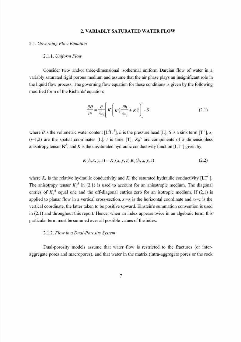
2. VARIABLY SATURATED WATER FLOW
2.1. Governing Flow Equation
2.1.1. Uniform Flow
Consider two- and/or three-dimensional isothermal uniform Darcian flow of water in a
variably saturated rigid porous medium and assume that the air phase plays an insignificant role in
the liquid flow process. The governing flow equation for these conditions is given by the following
modified form of the Richards' equation:
A Aij iz
i j
h= K + - S K K
t x x
θ ∂ ∂ ∂ ∂ ∂ ∂
(2.1)
where θ is the volumetric water content [L3L-3], h is the pressure head [L], S is a sink term [T-1], xi
(i=1,2) are the spatial coordinates [L], t is time [T], K ij A are components of a dimensionless
anisotropy tensor K A, and K is the unsaturated hydraulic conductivity function [LT-1] given by
( , , , ) ( , , ) ( , , , )s r K h x y z = K x y z K h x y z (2.2)
where K r is the relative hydraulic conductivity and K s the saturated hydraulic conductivity [LT-1
].The anisotropy tensor K ij
A in (2.1) is used to account for an anisotropic medium. The diagonal
entries of K ij A equal one and the off-diagonal entries zero for an isotropic medium. If (2.1) is
applied to planar flow in a vertical cross-section, x1= x is the horizontal coordinate and x2= z is the
vertical coordinate, the latter taken to be positive upward. Einstein's summation convention is used
in (2.1) and throughout this report. Hence, when an index appears twice in an algebraic term, this
particular term must be summed over all possible values of the index.
2.1.2. Flow in a Dual-Porosity System
Dual-porosity models assume that water flow is restricted to the fractures (or inter-
aggregate pores and macropores), and that water in the matrix (intra-aggregate pores or the rock
8/20/2019 HYDRUS3D Technical Manual.pdf
http://slidepdf.com/reader/full/hydrus3d-technical-manualpdf 38/260
8
matrix) does not move at all. These models assume that the matrix, consisting of immobile water
pockets, can exchange, retain, and store water, but does not permit convective flow. This
conceptualization leads to two-region, dual-porosity type flow and transport models [Philip,
1968; van Genuchten and Wierenga, 1976] that partition the liquid phase into mobile (flowing,
inter-aggregate), θ m, and immobile (stagnant, intra-aggregate), θ im, regions:
m im= +θ θ θ (2.3)
with some exchange of water and/or solutes possible between the two regions, usually calculated
by means of a first-order rate equation. We will use here the subscript m to represent fractures,
inter-aggregate pores, or macropores, and the subscript im to represent the soil matrix, intra-
aggregate pores, or the rock matrix.
The dual-porosity formulation for water flow as used in HYDRUS-1D is based on amixed formulation, which uses Richards equation (2.1) to describe water flow in the fractures
(macropores), and a simple mass balance equation to describe moisture dynamics in the matrix as
follows [Šimůnek et al., 2003]:
m A Aij iz m w
i j
im
im w
hK + S K K
t x x
S t
θ Γ
θ Γ
∂ ∂ ∂= − − ∂ ∂ ∂
∂= − +
∂
(2.4)
where S m and S im (S im is assumed to be zero in the current HYDRUS version) are sink terms for
both regions, and Γ w is the transfer rate for water from the inter- to the intra-aggregate pores.
An alternative dual-porosity approach, not implemented in HYDRUS-1D, was suggested
by Germann [1985] and Germann and Beven [1985], who used a kinematic wave equation to
describe gravitational movement of water in macropores. Although dual-porosity models have
been popularly used for solute transport studies (e.g. van Genuchten [1981]), they have not thus
far been used to water flow problems.
8/20/2019 HYDRUS3D Technical Manual.pdf
http://slidepdf.com/reader/full/hydrus3d-technical-manualpdf 39/260
9
2.2. Root Water Uptake
2.2.1. Root Water Uptake without Compensation
The sink term, S , in (2.1) represents the volume of water removed per unit time from a unitvolume of soil due to plant water uptake. Feddes et al. [1978] defined S as
( ) ( ) pS h = h S α (2.5)
where the water stress response function α (h) is a prescribed dimensionless function (Fig. 2.1) of
the soil water pressure head (0≤ α ≤1), and S p is the potential water uptake rate [T-1]. Figure 2.1
gives a schematic plot of the stress response function as used by Feddes et al. [1978]. Notice that
water uptake is assumed to be zero close to saturation (i.e., wetter than some arbitrary "anaerobiosis
point", h1). For h<h4 (the wilting point pressure head), water uptake is also assumed to be zero.Water uptake is considered optimal between pressure heads h2 and h3, whereas for pressure head
between h3 and h4 (or h1 and h2), water uptake decreases (or increases) linearly with h. The variable
S p in (2.5) is equal to the water uptake rate during periods of no water stress when α (h)=1. van
Genuchten [1987] expanded the formulation of Feddes by including osmotic stress as follows
( , ) ( ) pS h h = h, h S φ φ α (2.6)
where hφ is the osmotic head [L], which is assumed here to be given by a linear combination of theconcentrations, ci, of all solutes present, i.e.,
i ih = a c
φ (2.7)
in which ai are experimental coefficients [L4M] converting concentrations into osmotic heads. van
Genuchten [1987] proposed an alternative S-shaped function to describe the water uptake stress
response function (Fig. 2.1), and suggested that the influence of the osmotic head reduction can be
either additive or multiplicative as follows
8/20/2019 HYDRUS3D Technical Manual.pdf
http://slidepdf.com/reader/full/hydrus3d-technical-manualpdf 40/260
10
4
50
4
1( )
1
( , ) 0.
ph, h = h+ h h
h+ h+
h
h h = h+ h h
φ φ
φ
φ φ
α
α
>
<
(2.8)
or
1 2
50 50
1 1( , )
1 ( 1 () ) p p
h h =+ h/h + h /h
φ
φ φ
α (2.9)
respectively, where p, p1, and p2 are experimental constants. The exponent p was found to be
approximately 3 when applied to salinity stress data only [van Genuchten, 1987]. The parameter h50
in (2.8) and (2.9) represents the pressure head at which the water extraction rate is reduced by 50%
during conditions of negligible osmotic stress. Similarly, hφ 50 represents the osmotic head at which
the water extraction rate is reduced by 50% during conditions of negligible water stress. Note that,
in contrast to the expression of Feddes et al. [1978], this formulation of the stress response
function, α (h,hφ ), does not consider a transpiration reduction near saturation. Such a simplification
seems justified when saturation occurs for only relatively short periods of time. When the
multiplicative model is used for salinity stress, one can use the Threshold Model of Maas [1990]
as an alternative to the S-Shaped Model of van Genuchten [1985].
Note that different sensitivity of the root water uptake to water and salinity stresses can be
be considered using the additive formulation (2.8) as follows:
( )1 1
50 5050 50
1 1 1( , )
1 11
p p p
i i
h h
h a h h a a chh
h hh h
φ
φ φ
φ
α = = =
+ + + ++ +
(2.10)
where a1 is a coefficient accounting for different response to different stresses (=h50/hφ 50).
When the potential water uptake rate is equally distributed over a two-dimensional
rectangular root domain, S p becomes
1 p p t
x z
=S S T L L
(2.11)
where T p is the potential transpiration rate [LT-1
], L z is the depth [L] of the root zone, L x is thewidth [L] of the root zone, and S t is the width [L] of the soil surface associated with the
transpiration process. Notice that S p reduces to T p/ L z when S t = L x. For three-dimensional
problems, (2.11) additionally includes the width of the y-direction, L x [L], and S t becomes the soil
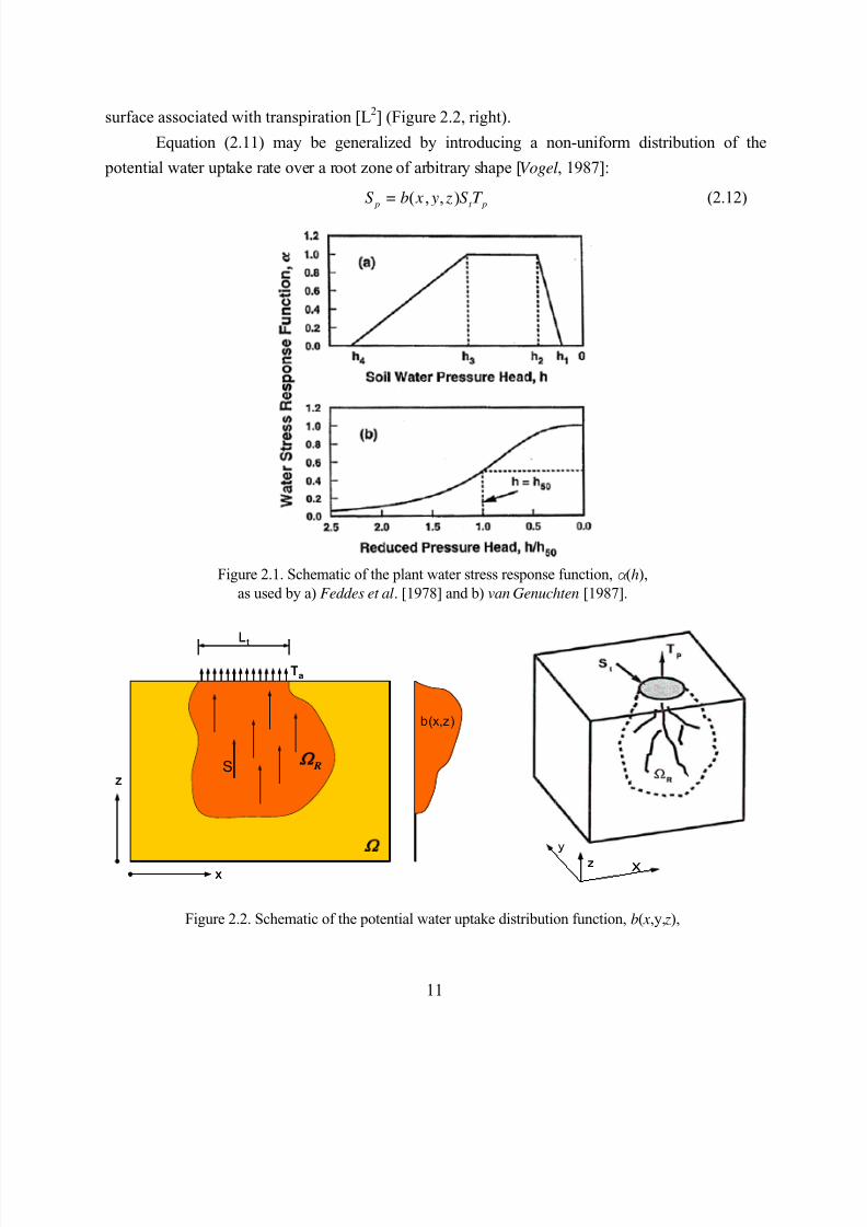
8/20/2019 HYDRUS3D Technical Manual.pdf
http://slidepdf.com/reader/full/hydrus3d-technical-manualpdf 41/260
11
surface associated with transpiration [L2] (Figure 2.2, right).
Equation (2.11) may be generalized by introducing a non-uniform distribution of the
potential water uptake rate over a root zone of arbitrary shape [Vogel, 1987]:
( , , ) p t pS = b x y z S T (2.12)
Figure 2.1. Schematic of the plant water stress response function, α (h),as used by a) Feddes et al. [1978] and b) van Genuchten [1987].
x
z
RS
Ta
Lt
b(x,z)
x
z
RS
Ta
Lt
b(x,z)
X
y
z X
y
z
Figure 2.2. Schematic of the potential water uptake distribution function, b( x,y, z),
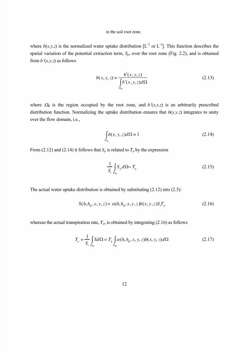
8/20/2019 HYDRUS3D Technical Manual.pdf
http://slidepdf.com/reader/full/hydrus3d-technical-manualpdf 42/260
12
in the soil root zone.
where b( x,y,z) is the normalized water uptake distribution [L-2 or L-3]. This function describes the
spatial variation of the potential extraction term, S p, over the root zone (Fig. 2.2), and is obtained
from b’( x,y,z) as follows
( , , )( , , )
( , , ) R
b x y zb x y z =
b x y z d Ω
′
′ Ω∫ (2.13)
where Ω R is the region occupied by the root zone, and b’( x,y,z) is an arbitrarily prescribed
distribution function. Normalizing the uptake distribution ensures that b( x,y,z) integrates to unity
over the flow domain, i.e.,
( , , ) 1 R
b x y z d =Ω
Ω∫ (2.14)
From (2.12) and (2.14) it follows that S p is related to T p by the expression
1
R
p pt
S d T S Ω
Ω=∫ (2.15)
The actual water uptake distribution is obtained by substituting (2.12) into (2.5):
( , , , , ) ( , , , ) ( , , ) t pS h h x y z = h,h x y z b x y z S T φ φ α (2.16)
whereas the actual transpiration rate, T a, is obtained by integrating (2.16) as follows
1( , , , , ) ( , , )
R R
a pt
T = Sd = T h h x y z b x y z d S φ α
Ω Ω
Ω Ω∫ ∫ (2.17)
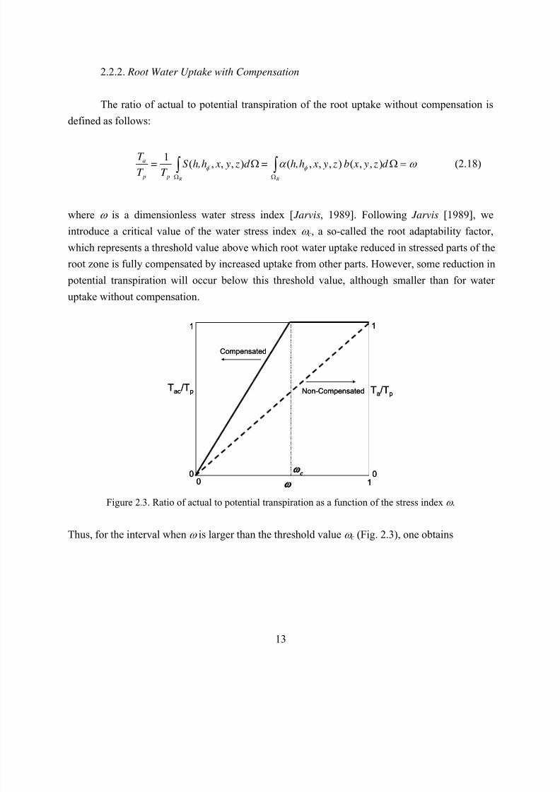
8/20/2019 HYDRUS3D Technical Manual.pdf
http://slidepdf.com/reader/full/hydrus3d-technical-manualpdf 43/260
13
2.2.2. Root Water Uptake with Compensation
The ratio of actual to potential transpiration of the root uptake without compensation is
defined as follows:
1( , , , ) ( , , , ) ( , , )
R R
a
p p
T = S h,h x y z d = h,h x y z b x y z d
T T φ φ α ω
Ω Ω
Ω Ω =∫ ∫ (2.18)
where ω is a dimensionless water stress index [ Jarvis, 1989]. Following Jarvis [1989], we
introduce a critical value of the water stress index ω c, a so-called the root adaptability factor,
which represents a threshold value above which root water uptake reduced in stressed parts of the
root zone is fully compensated by increased uptake from other parts. However, some reduction in
potential transpiration will occur below this threshold value, although smaller than for wateruptake without compensation.
00
1
10
1
Tac/Tp Ta/Tp
c
Compensated
Non-Compensated
00
1
10
1
Tac/Tp Ta/Tp
c
Compensated
Non-Compensated
Figure 2.3. Ratio of actual to potential transpiration as a function of the stress index ω .
Thus, for the interval when ω is larger than the threshold value ω c (Fig. 2.3), one obtains
8/20/2019 HYDRUS3D Technical Manual.pdf
http://slidepdf.com/reader/full/hydrus3d-technical-manualpdf 44/260
14
( , , , ) ( , , , ) ( , , )
( , , , ) ( , , )
1 R
p
La
p
T S h,h x y z = h,h x y z b x y z
h,h x y z b x y z dxT
=
T
φ φ
φ
α ω
α ω
ω ω
= =∫ (2.19)
While for the interval when ω is smaller than the threshold value ω c, one has
( , , ) ( , , , ) ( , , )
( , , , ) ( , , )
1 R
p
c
La
p c c
T S h,h ,x y z = h,h x y z b x y z
h,h x y z b x y z dx
T =
T
φ φ
φ
α ω
α ω
ω ω = <
∫ (2.20)
When the parameter ω c is equal to one we hence have noncompensated root water uptake, and
when ω c is equal to zero we obtain fully compensated uptake.
2.2.3. Spatial Root Distribution Functions
Following two- and three-dimensional root distribution functions are implemented into
HYDRUS [Vrught et al., 2001, 2002]:
( )* *
, 1 1 z r
m m
p p z z x x
Z X
m m
z xb x z e
Z X
− − + −
= − −
(2.21)
( )* * *
, , 1 1 1 y x z
m m m
p p p x x y y z z
X Y Z
m m m
x y zb x y z e
X Y Z
− − + − + −
= − − −
(2.22)
where X m, Y m, and Z m are the maximum rooting lengths in the x-, y-, and z- directions [L],
respectively; x, y, and z are distances from the origin of the tree in the x-, y-, and z- directions [L],respectively; p x [-], p y [-], p z [-], x
* [L], y* [L], and z* [L] are empirical parameters, and b( x, z) and
b( x, y, z) denote two- and three-dimensional spatial distribution of the potential root water uptake
[-]. Following Vrught et al. [2002], we set p x, p y and p z to unity for z> z*, x> x* and y> y*,
8/20/2019 HYDRUS3D Technical Manual.pdf
http://slidepdf.com/reader/full/hydrus3d-technical-manualpdf 45/260
15
respectively. Vrugt et al. [2001ab] showed that the root water uptake in (2.21) is extremely
flexible and allows spatial variations of water uptake as influenced by non-uniform water
application (e.g. drip irrigation) and root length density patterns. See Vrugt et al. [2001ab] for
different configurations of normalized spatial distribution of potential root water uptake.
2.3. The Unsaturated Soil Hydraulic Properties
The unsaturated soil hydraulic properties, θ (h) and K (h), in (2.1) are in general highly
nonlinear functions of the pressure head. HYDRUS permits the use of five different analytical
models for the hydraulic properties [ Brooks and Corey, 1964; van Genuchten, 1980; and Vogel and
Císlerová, 1988; Kosugi, 1995, Durner , 1994].
The soil water retention, θ (h), and hydraulic conductivity, K (h), functions according to
Brooks and Corey [1964] are given by
1
1 1
-n
e
h < - / | h |S =
h - /
α α
α
≥ (2.23)
2 2 / n+l+
s eK = K S (2.24)
respectively, where S e is the effective water content,
-
-r
e
s r
S θ θ
θ θ = (2.25)
in which θ r and θ s denote the residual and saturated water content, respectively; K s is the saturated
hydraulic conductivity, α is the inverse of the air-entry value (or bubbling pressure), n is a pore-size
distribution index, and l is a pore-connectivity parameter assumed to be 2.0 in the original study of
Brooks and Corey [1964]. The parameters α, n and l in HYDRUS are considered to be merelyempirical coefficients affecting the shape of the hydraulic functions.
HYDRUS also implements the soil-hydraulic functions of van Genuchten [1980] who used
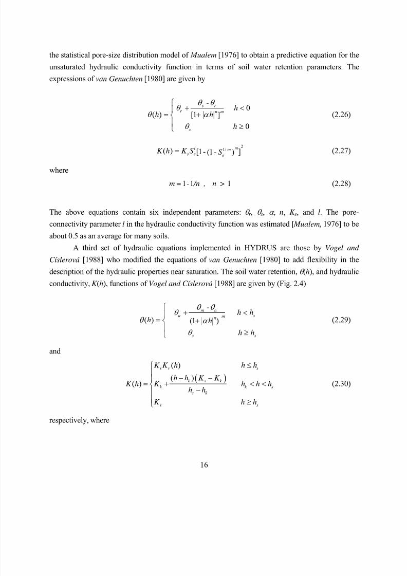
8/20/2019 HYDRUS3D Technical Manual.pdf
http://slidepdf.com/reader/full/hydrus3d-technical-manualpdf 46/260
16
the statistical pore-size distribution model of Mualem [1976] to obtain a predictive equation for the
unsaturated hydraulic conductivity function in terms of soil water retention parameters. The
expressions of van Genuchten [1980] are given by
- 0( ) [1 | | ]
0
s r
r n m
s
hh h
h
θ θ θ
θ α
θ
+ <= +
≥
(2.26)
21/( ) [1- ](1- )
ml ms e e
K h K S S = (2.27)
where
1 1 1m = - /n , n > (2.28)
The above equations contain six independent parameters: θ r , θ s, α , n, K s, and l. The pore-
connectivity parameter l in the hydraulic conductivity function was estimated [ Mualem, 1976] to be
about 0.5 as an average for many soils.
A third set of hydraulic equations implemented in HYDRUS are those by Vogel and
Císlerová [1988] who modified the equations of van Genuchten [1980] to add flexibility in the
description of the hydraulic properties near saturation. The soil water retention, θ (h), and hydraulic
conductivity, K (h), functions of Vogel and Císlerová [1988] are given by (Fig. 2.4)
-
( ) (1 | )|
m a
a smn
s s
h hh h
h h
θ θ θ
θ α
θ
+ <
= + ≥
(2.29)
and
( )
( )
( )( )
s r s
k s k
k k s
s k
s s
K K h h h
h h K K K h K h h h
h h
K h h
≤
− −= + < <
−
≥
(2.30)
respectively, where
8/20/2019 HYDRUS3D Technical Manual.pdf
http://slidepdf.com/reader/full/hydrus3d-technical-manualpdf 47/260
17
( ) ( )
( ) ( )
21/ 2
r k er
s ek r k
F F K S K
K S F F
θ θ
θ θ
− = −
(2.31)
( )
1/
1
mm
a
m a
F θ θ θ θ θ
− = −
− (2.32)
k r
ek
s r
S θ θ
θ θ
−=
− (2.33)
The above equations allow for a non-zero minimum capillary height, hs, by replacing the parameter
θ s in van Genuchten's retention function by a fictitious (extrapolated) parameter θ m slightly larger
than θ s as shown in Figure 2.4. While this change from θ s to θ m has little or no effect on theretention curve, the effect on the shape and value of the hydraulic conductivity function can be
considerable, especially for fine-textured soils when n is relatively small (e.g., 1.0 < n < 1.3). To
increase the flexibility of the analytical expressions, the parameter θ r in the retention function was
replaced by the fictitious (extrapolated) parameter θ a≤ θ r . The approach maintains the physical
meaning of θ r and θ s as measurable quantities. Equation (2.31) assumes that the predicted hydraulic
conductivity function is matched to a measured value of the hydraulic conductivity, K k =K (θ k ), at
some water content, θ k , less that or equal to the saturated water content, i.e., θ k ≤ θ s and K k ≤K s [Vogel
and Císlerová, 1988; Luckner et al., 1989]. Inspection of (2.29) through (2.31) shows that the
hydraulic characteristics contain 9 unknown parameters: θ r , θ s, θ a, θ m, α , n, K s , K k , and θ k . When
θ a=θ r , θ m=θ k =θ s and K k =K s , the soil hydraulic functions of Vogel and Císlerová [1988] reduce to
the original expressions of van Genuchten [1980].
8/20/2019 HYDRUS3D Technical Manual.pdf
http://slidepdf.com/reader/full/hydrus3d-technical-manualpdf 48/260
18
Figure 2.4. Schematics of the soil water retention (a) and hydraulic conductivity (b) functionsas given by equations (2.29) and (2.30), respectively.
Version 3.0 of Hydrus allows the soil hydraulic properties to be defined also acoording to
Kosugi [1996], who suggested the following lognormal distribution model for S e(h):
( )ln /1( 0)
2 2
1 ( 0)
r e
s r
herfc h
S n
h
α θ θ
θ θ
<−
= = − ≥
(2.34)
Application of Mualem's pore-size distribution model [ Mualem, 1976] now leads to the
following hydraulic conductivity function:
8/20/2019 HYDRUS3D Technical Manual.pdf
http://slidepdf.com/reader/full/hydrus3d-technical-manualpdf 49/260
19
( )2
1/ 2ln /1
( 0)2 2 2
( 0)
s e
s
h nK S erfc h
K n
K h
α + < =
≥
(2.35)
Note that in in this text we use symbols α instead of h0 and n instead of σ as used in Kosugi
[1996].
Durner [1994] divided the porous medium into two (or more) overlapping regions and
suggested to use for each of these regions a van Genuchten-Mualem type function [van
Genuchten, 1980] of the soil hydraulic properties. Linear superposition of the functions for each
particular region gives then the functions for the composite multimodal pore system [ Durner et
al., 1999]:
1 1 2 2
1 1 2 2= [1 ( ) ] [1 ( ) ]n -m n -me w + h w + hS α α + (2.36)
Combining this retention model with Mualem’s [1976] pore-size distribution model leads now to:
K S = K
w S w S w - - S w - - S
w we s
e e
l m
e / m m
e / m
( )[ ( ) ] [ ( ) ]1 2 1 1
12 2
12
1 1 2 2
2
1 2
1
1
1 2
2
21 1 1 1+ +
+
d i e jb g
α α
α α (2.37)
where wi are the weighting factors for the two overlapping regions, and α i, ni, mi (=1-1/ni), and l
are empirical parameters of the separate hydraulic functions (i=1,2).
An example of composite retention and hydraulic conductivity functions for two
overlapping porous media is shown in Figure 2.5. Note that the pressure head axes are on a log
scale, which causes the near-saturated values to be significantly enlarged. The fracture domain in
this example represents only 2.5% of the entire pore space, but accounts for almost 90% of the
hydraulic conductivity close to saturation. Curves similar to those in Figure 2.5 have been used
also for fractured rock by Peters and Klavetter [1988], Pruess and Wang [1987], and Flint et al. [2001], among others.
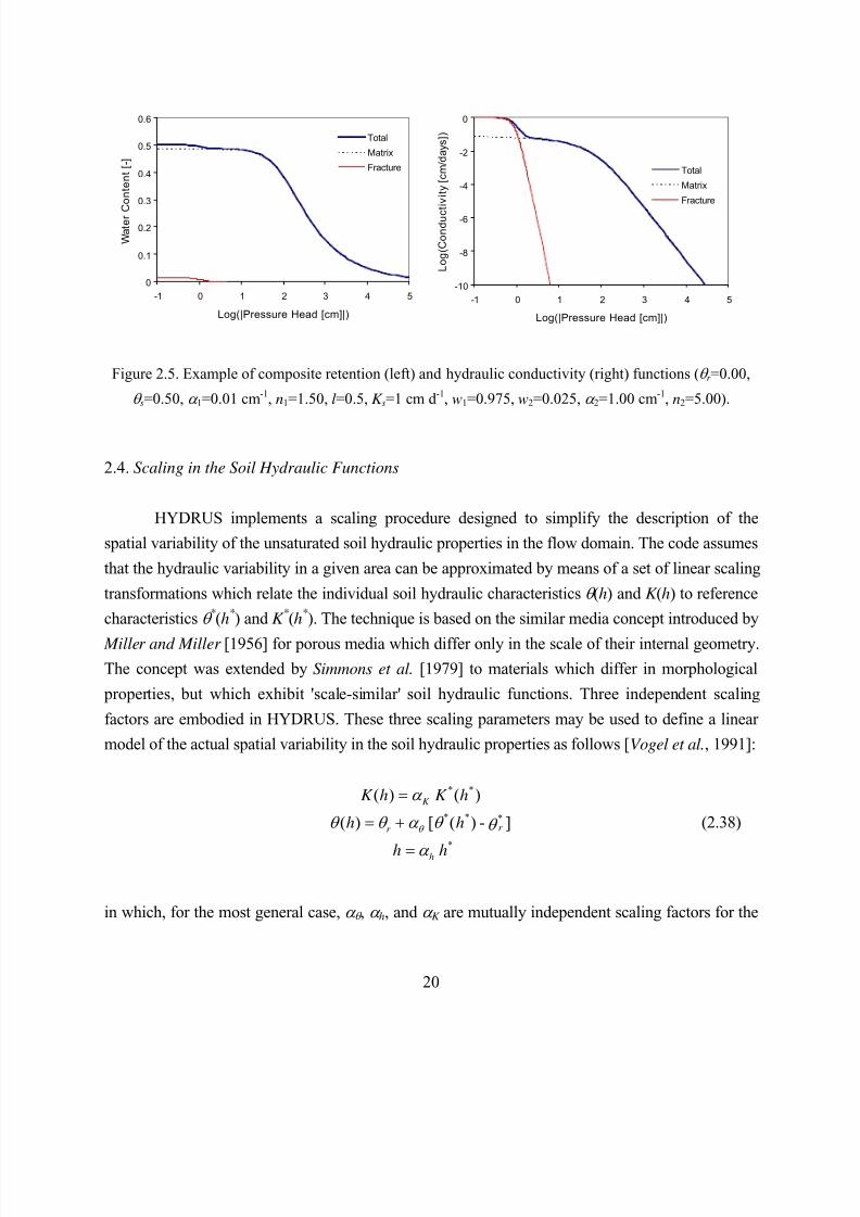
8/20/2019 HYDRUS3D Technical Manual.pdf
http://slidepdf.com/reader/full/hydrus3d-technical-manualpdf 50/260
20
0
0.1
0.2
0.3
0.4
0.5
0.6
-1 0 1 2 3 4 5
Log(|Pressure Head [cm]|)
W a t e r C o n t e n t [ - ]
Total
Matrix
Fracture
-10
-8
-6
-4
-2
0
-1 0 1 2 3 4 5
Log(|Pressure Head [cm]|)
L o g ( C o n d u c
t i v i t y [ c m / d a y s ] )
Total
Matrix
Fracture
Figure 2.5. Example of composite retention (left) and hydraulic conductivity (right) functions (θ r =0.00,
θ s=0.50, α 1=0.01 cm-1, n1=1.50, l=0.5, K s=1 cm d-1, w1=0.975, w2=0.025, α 2=1.00 cm-1, n2=5.00).
2.4. Scaling in the Soil Hydraulic Functions
HYDRUS implements a scaling procedure designed to simplify the description of the
spatial variability of the unsaturated soil hydraulic properties in the flow domain. The code assumes
that the hydraulic variability in a given area can be approximated by means of a set of linear scaling
transformations which relate the individual soil hydraulic characteristics θ (h) and K (h) to reference
characteristics θ *(h*) and K *(h*). The technique is based on the similar media concept introduced by
Miller and Miller [1956] for porous media which differ only in the scale of their internal geometry.The concept was extended by Simmons et al. [1979] to materials which differ in morphological
properties, but which exhibit 'scale-similar' soil hydraulic functions. Three independent scaling
factors are embodied in HYDRUS. These three scaling parameters may be used to define a linear
model of the actual spatial variability in the soil hydraulic properties as follows [Vogel et al., 1991]:
* *
* * *
*
( ) ( )
( ) [ ( ) - ]
K
r r
h
K h K h
h h
h h
θ
α
θ θ α θ θ
α
=
= +
=
(2.38)
in which, for the most general case, α θ , α h, and α K are mutually independent scaling factors for the
8/20/2019 HYDRUS3D Technical Manual.pdf
http://slidepdf.com/reader/full/hydrus3d-technical-manualpdf 51/260
21
water content, the pressure head and the hydraulic conductivity, respectively. Less general scaling
methods arise by invoking certain relationships between α θ , α h and/or α K . For example, the original
Miller-Miller scaling procedure is obtained by assuming α θ =1 (with θ r * = θ r ), and α K =α h-2. A
detailed discussion of the scaling relationships given by (2.38), and their application to the
hydraulic description of heterogeneous soil profiles, is given by Vogel et al. [1991].
2.5. Temperature Dependence of the Soil Hydraulic Functions
A similar scaling technique as described above is used in HYDRUS to express the
temperature dependence of the soil hydraulic functions. Based on capillary theory that assumes that
the influence of temperature on the soil water pressure head can be quantitatively predicted from the
influence of temperature on surface tension, Philip and de Vries [1957] derived the following
equation
dh h d =
dT dT
σ
σ (2.39)
where T is temperature [K] and σ is the surface tension at the air-water interface [MT-2]. From
(2.39) it follows that
*T T ref h ref
ref h = h = h
σ
α σ (2.40)
where hT and href (σ T and σ ref ) are pressure heads (surface tensions) at temperature T and reference
temperature T ref , respectively; and α h* is the temperature scaling factor for the pressure head.
Following Constantz [1982], the temperature dependence of the hydraulic conductivity can
be expressed as
*( ) ( ) ( )ref
T T ref K ref
T ref
K K K µ ρ
θ θ α θ µ ρ = = (2.41)
8/20/2019 HYDRUS3D Technical Manual.pdf
http://slidepdf.com/reader/full/hydrus3d-technical-manualpdf 52/260
22
where K ref and K T denote hydraulic conductivities at the reference temperature T ref and soil
temperature T , respectively; µ ref and µ T ( ρ ref and ρ T ) represent the dynamic viscosity [ML-1T-1]
(density of soil water [ML-3]) at temperatures T ref and T , respectively; and α K * is the temperature
scaling factor for the hydraulic conductivity.
2.6. Hysteresis in the Soil Hydraulic Properties
Applications of unsaturated flow models often assume unique, single-valued (non-
hysteretic) functions for θ (h) and K (h) to characterize the hydraulic properties at a certain point in
the soil profile. While such a simplification may be acceptable for some flow simulations, many
cases require a more realistic description involving hysteresis in the soil hydraulic properties. The
HYDRUS code incorporates hysteresis by using the empirical model introduced by Scott et al.
[1983]. This model was also employed by Kool and Parker [1987], who modified the formulation
to account for air entrapment. The present version of HYDRUS further extends the model of Kool
and Parker according to Vogel et al. [1996] by considering also hysteresis in the hydraulic
conductivity function.
The adopted procedure for modeling hysteresis in the retention function requires that both
the main drying and main wetting curves be known (Fig. 2.6). These two curves are described with
(2.27) using the parameter vectors (θ r d , θ s
d , θ md , α
d , nd ) and (θ r w, θ s
w, θ mw, α
w, nw), respectively,
where the subscripts d and w indicate wetting and drying, respectively. The following restrictions
are expected to hold in most practical applications:
,d w d w
r r =θ θ α α ≤ (2.42)
We also invoke the often-assumed restriction
d wn n= (2.43)
If data are lacking, one may use α w = 2α d as a reasonable first approximation [Kool and Parker ,1987; Nielsen and Luckner , 1992]. We further assume
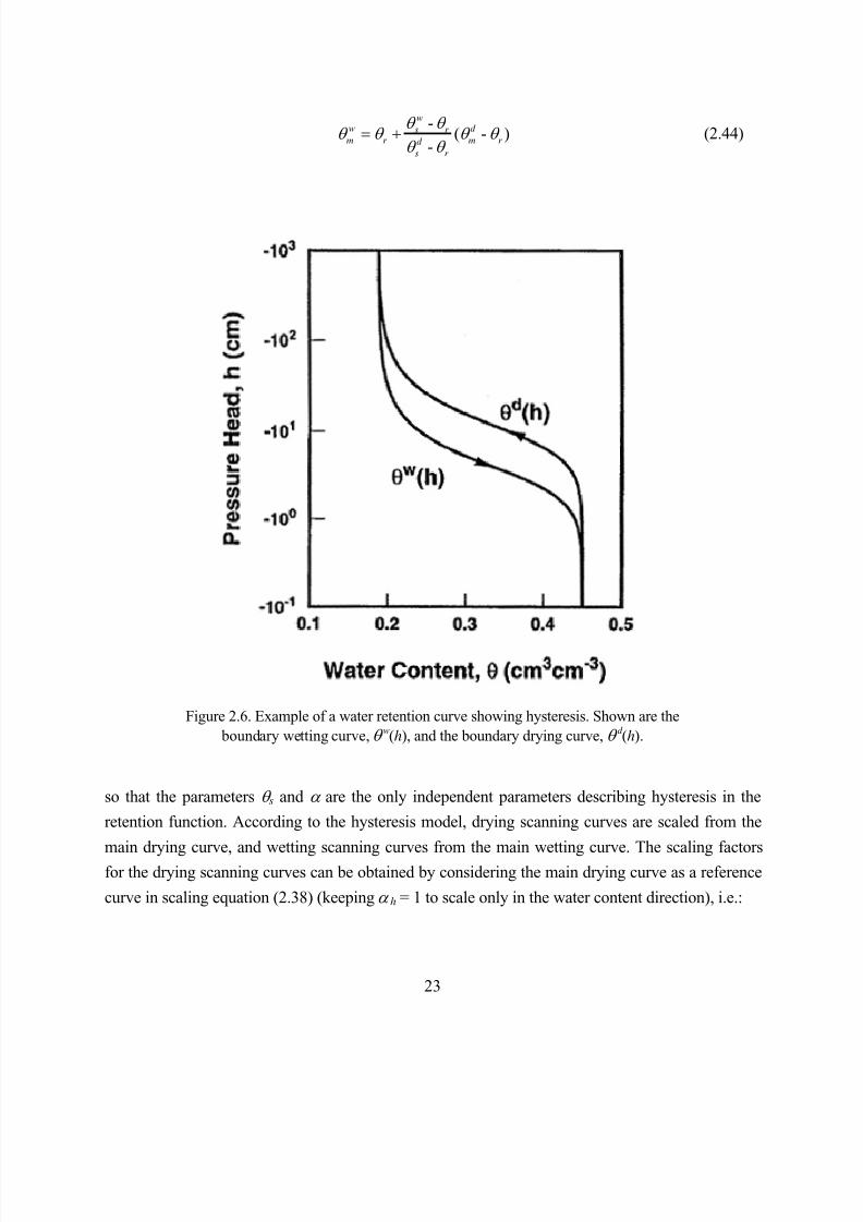
8/20/2019 HYDRUS3D Technical Manual.pdf
http://slidepdf.com/reader/full/hydrus3d-technical-manualpdf 53/260
23
-( - )
-
ww d s r m r m r d
s r
θ θ
θ θ θ θ θ θ
= + (2.44)
Figure 2.6. Example of a water retention curve showing hysteresis. Shown are the boundary wetting curve, θ w(h), and the boundary drying curve, θ d (h).
so that the parameters θ s and α are the only independent parameters describing hysteresis in the
retention function. According to the hysteresis model, drying scanning curves are scaled from the
main drying curve, and wetting scanning curves from the main wetting curve. The scaling factors
for the drying scanning curves can be obtained by considering the main drying curve as a reference
curve in scaling equation (2.38) (keeping α h = 1 to scale only in the water content direction), i.e.:
8/20/2019 HYDRUS3D Technical Manual.pdf
http://slidepdf.com/reader/full/hydrus3d-technical-manualpdf 54/260
24
'( ) [ ( ) - ]d d
r r h hθ θ θ α θ θ = + (2.45)
and forcing each scanning curve, θ (h), to pass through the point (θ ∆, h∆) characterizing the latest
reversal from wetting to drying. Substituting this reversal point into (2.45), and assuming thatθ r = θ r
d , leads to
-
( ) -r
d
r h
θ
θ θ α
θ θ ∆
∆
= (2.46)
Note that the scaling procedure results in a fictitious value of the parameter θ s’ for the drying
scanning curve (this parameter may be located outside of the main hysteresis loop). The scaling
relationship is similarly for the wetting scanning curves
'( ) [ ( ) - ]w
r r h h
θ θ θ α θ θ = + (2.47)
in which the fictitious parameter θ r ’ is now used (again possibly scaled outside of the main loop).
The scaling factor αθ for a particular scanning curve can be obtained by substituting the reversal
point (θ ∆, h∆) and the full saturation point (θ s, 0) into (2.47), and subtracting the two resulting
equations to eliminate θ r ’ to give
-
( ) -s
w w
sh
θ
θ θ α
θ θ ∆
∆
= (2.48)
The parameter θ r ’ is subsequently determined from (2.47) as θ r ’ = θ s - α θ (θ sw - θ r ). If the main
hysteresis loop is not closed at saturation, the water content at saturation for a particular wetting
scanning curve is evaluated using the empirical relationship of Aziz and Settari [1979]
- 1 1- , -1 ( - ) - -
d
d ss s d d w d d
s s s s r
R Rθ θ θ θ
θ θ θ θ θ θ ∆
∆
= =+
(2.49)
8/20/2019 HYDRUS3D Technical Manual.pdf
http://slidepdf.com/reader/full/hydrus3d-technical-manualpdf 55/260
25
An analogous hysteretic procedure can be applied to the unsaturated hydraulic conductivity
function K (h). The main branches K d (h) and K w(h) of the hysteresis loop are characterized by the
same set of parameters as the corresponding retention curves θ d (h) and θ
w(h), and by the saturated
conductivities K sd and K s
w according to Eq. (2.27). For drying scanning curves we obtain from
(2.38)
( ) ( )d
K K h K hα = (2.50)
From knowledge of the reversal point (h∆ , K ∆) we obtain
( )K d
K
K hα ∆
∆
= (2.51)
For a wetting scanning curve we have now
'( ) ( )w
r K K h K K hα = + (2.52)
where K r ’ is a fictitious parameter. Substituting the reversal point (h∆ , K ∆) and the saturation point
(0, K s) into (2.40) and solving for α K yields
( )s
K w ws
K - K =
K h - K α ∆
∆
(2.53)
The fictitious conductivity parameter K r ’ may be obtained from (2.52) as K r ’ = K s - α K K sw. If the
main hysteresis loop is not closed at saturation, the hydraulic conductivity at saturation for a wetting
scanning curve is evaluated using equations similar to (2.49), i.e.,
- 1 1- , -1 ( - ) -
d
d ss s d d w d
s s s s
K K K K R R K K K K K
∆
∆
= =+
(2.54)
8/20/2019 HYDRUS3D Technical Manual.pdf
http://slidepdf.com/reader/full/hydrus3d-technical-manualpdf 56/260
26
While relatively simple to implement, the above model has been found to suffer from a
so-called pumping effect, in which the hysteresis loops can move to physically unrealistic parts
of the retention function. As an alternative, we also incorporated in HYDRUS the hysteresis
model of Lenhard et al. [1991] and Lenhard and Parker [1992] that eliminates pumping by
keeping track of historical reversal points. We greatly acknowledge the help of Robert Lenhard inthis effort.
2.7. Initial and Boundary Conditions
The solution of Eq. (2.1) requires knowledge of the initial distribution of the pressure head
or the water content within the flow domain, Ω :
0
0
( , , , ) ( , , ) for = 0
( , , , ) ( , , ) for = 0
h x y z t = h x y z t
x y z t = x y z t θ θ (2.55)
where h0 is a prescribed function of x, y and z. Initial condition can also be set (in the graphical
user interface) to be equal to water content at field capacity, which is calculated as follows
[Twarakavi et al., 2009]:
( )( )sK
r s
r fc fc nS 10log260.0 +−=
−−=
θ θ θ θ (2.56)
where θ fc and S fc are the water content and saturation at field capacity, and θ r , θ s, n, and K s are the
soil hydraulic parameters for the van Genuchten [1980] model. Note that the water content at
field capacity corresponds to the hydraulic conductivity of about 0.01 cm/d [Twarakavi et al.,
2009]. The initial pressure head at field capacity is calculated from the water content at field
capacity using the the van Genuchten [1980] retention curve model.
2.7.1. System-Independent Boundary Conditions
HYDRUS implements three types of conditions to describe system-independent interactions
8/20/2019 HYDRUS3D Technical Manual.pdf
http://slidepdf.com/reader/full/hydrus3d-technical-manualpdf 57/260
27
along the boundaries of the flow region. These conditions are specified pressure head (Dirichlet
type) boundary conditions of the form
( , , , ) ( , , , ) for ( , , ) Dh x y z t = x y z t x y zψ ∈ Γ (2.57)
specified flux (Neumann type) boundary conditions given by
1[ ( )] ( , , , ) for ( , , ) A A N ij iz i
j
h- K K + K n = x y z t x y z
xσ
∂∈ Γ
∂ (2.58)
and specified gradient boundary conditions
2( )] ( , , , ) for ( , , ) A Agij iz i
j
hK + K n = x y z t x y z
xσ
∂∈ Γ
∂ (2.59)
where Γ D, Γ N , and Γ G indicate Dirichlet, Neumann, and gradient type boundary segments,
respectively; ψ [L], σ 1 [LT-1], and σ 2 [-] are prescribed functions of x, z and t ; and ni are the
components of the outward unit vector normal to boundary Γ N or Γ G. As pointed out by McCord
[1991], the use of the term "Neumann type boundary condition" for the flux boundary is not very
appropriate since this term should hold for a gradient type condition (see also Section 3.2 for solutetransport). However, since the use of the Neumann condition is standard in the hydrologic literature
[ Neuman, 1972; Neuman et al., 1974], we shall also use this term to indicate flux boundaries
throughout this report. HYDRUS implements the gradient boundary condition only in terms of a
unit vertical hydraulic gradient simulating free drainage from a relatively deep soil profile. This
situation is often observed in field studies of water flow and drainage in the vadose zone [Sisson,
1987; McCord , 1991]. McCord [1991] states that the most pertinent application of (2.59) is its use
as a bottom outflow boundary condition for situations where the water table is situated far below
the domain of interest.
8/20/2019 HYDRUS3D Technical Manual.pdf
http://slidepdf.com/reader/full/hydrus3d-technical-manualpdf 58/260
28
2.7.2. System-Dependent Boundary Conditions
2.7.2.1. Atmospheric Boundary Conditions
In addition to the system-independent boundary conditions given by (2.57), (2.58), and (2.
59), HYDRUS considers several different types of system-dependent boundary conditions whichcannot be defined a priori. One of these involves soil-air interfaces, which are exposed to
atmospheric conditions. The potential fluid flux across these interfaces is controlled exclusively by
external conditions. However, the actual flux depends also on the prevailing (transient) soil
moisture conditions. Soil surface boundary conditions may change from prescribed flux to
prescribed head type conditions (and vice-versa). In the absence of surface ponding, the numerical
solution of (2.1) is obtained by limiting the absolute value of the flux such that the following two
conditions are satisfied [ Neuman et al., 1974]:
( ) A A
ij iz i
j
h| K K + K n | E x∂ ≤∂
(2.60)
and
A S h h h≤ ≤ (2.61)
where E is the maximum potential rate of infiltration or evaporation under the current atmospheric
conditions, h is the pressure head at the soil surface, and h A and hS are, respectively, minimum and
maximum pressure heads allowed under the prevailing soil conditions. The value for h A is
determined from the equilibrium conditions between soil water and atmospheric water vapor,
whereas hS is usually set equal to zero. HYDRUS assumes that any excess water on the soil surface
is immediately removed. When one of the end points of (2.61) is reached, a prescribed head
boundary condition will be used to calculate the actual surface flux. Methods of calculating E and
h A on the basis of atmospheric data have been discussed by Feddes et al. [1974].
2.7.2.2. Seepage Face
A second type of system-dependent boundary condition considered in HYDRUS is a
seepage face through which water leaves the saturated part of the flow domain. In this case, the
length of the seepage face is not known a priori. HYDRUS assumes that the pressure head is always
uniformly equal to zero along a seepage face. Additionally, the code assumes that water leaving the
8/20/2019 HYDRUS3D Technical Manual.pdf
http://slidepdf.com/reader/full/hydrus3d-technical-manualpdf 59/260
29
saturated zone across a seepage face is immediately removed by overland flow or some other
removal process. In Version 2.0, users can specify the pressure head other than zero for activating
the seepage face.
2.7.2.3. Tile Drains
A third class of system-dependent boundary conditions in HYDRUS concerns tile drains.
Similarly as for seepage phase, HYDRUS assumes that as long as a drain is located in the saturated
zone, the pressure head along the drain will be equal to zero; the drain then acts as a pressure head
sink. However, the drain will behave as a nodal sink/source with zero recharge when located in the
unsaturated zone. More information can be found in Section 5.3.7.
2.7.2.4. Special Time-Variable Flux/Head Boundary Conditions
In addition to system-dependent boundary conditions available in version 2.x of HYDRUS-2D,
several new options are available in HYDRUS:
a) While in earlier versions, all boundary conditions (i.e., fluxes or pressure heads) changed
in abrupt steps, the new version allows boundary pressure heads to change smoothly with
time. Abrupt changes in the pressure heads lead to sudden changes in fluxes, while
smoothly changing pressure heads provide smoothly changing fluxes. An example of
such a boundary condition is the water level in a stream or furrow.
b) While earlier versions only allowed either time-variable pressure heads or time-variable
fluxes on a particular part of the boundary, the new version allows boundary conditions to
change from variable pressure heads to a zero flux and vice-versa. This boundary
condition can be used for example for a disc permeameter where the specified head
changes to a zero flux during time periods when the permeameter is re-supplied with
water. The zero flux is initiated by specifying a value larger than 999999.
c) When a time-variable pressure head boundary condition is specified along a boundary,
then the specified value is assigned to the lowest nodal point of a particular boundary,
while pressure heads at other nodes are adjusted based on the z-coordinate. When thisoption is selected, then nodes with calculated negative pressure heads are not associated
with a Dirichlet boundary condition, but rather with a zero flux. A fluctuating water level
in a stream or furrow is an example of this type of boundary condition. While positive
8/20/2019 HYDRUS3D Technical Manual.pdf
http://slidepdf.com/reader/full/hydrus3d-technical-manualpdf 60/260
30
pressure head values are below the water table, negative values occur above the water
table.
d) This is similar to c) except that an atmospheric boundary condition is assigned to nodes
with negative calculated pressure heads.
e) This is similar to c) except that a seepage face boundary condition is assigned to nodeswith negative calculated pressure heads.
f) When this type of system-dependent boundary condition is selected, then HYDRUS treats
the time-variable flux boundary conditions similarly as atmospheric fluxes. This means
that pressure heads have two limiting values, with the maximum pressure head equal to
hCritS and the minimum pressure head equal to hCritA.
g) While in earlier versions of the code, the flux across the nonactive part of the seepage
face was always equal to zero, the new version can apply atmospheric boundary
conditions on a nonactive seepage face.Boundary condition options a) through g) can be used only with the first time-variable head/flux
condition.
2.7.2.5. Snow Boundary Condition
When heat transport is simulated simultaneously with water flow and atmospheric
boundary conditions, then snow accumulation on top of the soil surface can be simulated. The
code then assumes that when the air temperature is below -2 C all precipitation is in the form of
snow. When the air temperature is above +2 C all precipitation is in the form of liquid, while a
linear transition is used between the two limiting temperatures (-2,2). The code further assumesthat when the air temperature is above zero, the existing snow layer (if it exists) melts
proportionally to the air temperature.
2.7.2.6. Gradient-Type Boundary Condition
Version 1.xx of HYDRUS implements gradient type boundary condition only as the Free
Drainage boundary condition, or the unit gradient boundary condition. However, in many
situations one needs a non-unit gradient BC. For example, it is difficult to select appropriate
boundary conditions for vertical boundaries for flow in a hill slope where the side-gradient is
more or less parallel with the direction of the slope. We have implemented in Version 2.0 ofHYDRUS an option, using which users can specify a gradient other than one (unit gradient). This
option, i.e., non-unit gradient boundary condition, needs to be selected from the Special
8/20/2019 HYDRUS3D Technical Manual.pdf
http://slidepdf.com/reader/full/hydrus3d-technical-manualpdf 61/260
31
Boundary Conditions tab of the Boundary Conditions Options dialog window. Gradients are
positive for flow against a particular axis, i.e., from right to left (in the x-direction) and from back
to front (in the y-direction), and should be used only (or mainly) on sides of the transport domain.
In 3D, gradient BCs can be specified only in one direction (i.e., in either x- or y-direction).
2.7.2.7. Subsurface Drip Characteristic Function
Infiltration rate of water from a subsurface cavity (dripper) is affected by many factors,
including the pressure in the cavity, its size and geometry, and the hydraulic properties of the
surrounding soil [ Lazarovitch et al., 2005]. When a predetermined discharge of a subsurface
source (e.g., a subsurface emitter) is larger than the soil infiltration capacity, the pressure head in
the source outlet increases and becomes positive. The built up pressure may significantly reduce
the source discharge rate. HYDRUS implements a special system-dependent boundary condition
for flow from subsurface sources that uses the drip characteristic function:
( )0= -c
in sQ Q h h (2.62)
where hs [L] is the pressure head at the source-soil interface, often called the back pressure, Q0
[L3T-1] ([L2T-1] in 2D) is the nominal discharge (Optimal Flux in the HYDRUS GUI) of the
source for the reference inlet pressure hin (usually being 10 m) and the back pressure equal to
zero, Q [L3T-1] ([L2T-1] in 2D) is the source discharge for the actual back pressure hs, and c [-] is
an empirical constant (Exponent in the HYDRUS GUI) that reflects the flow characteristics of the
emitter. Normally, c = 0.5 corresponds to a turbulent flow emitter and c = 1 to a laminar one. This
equation states that when hs increases, the pressure difference between the soil and the source
inlet decreases and the discharge rate correspondingly decreases [ Lazarovitch et al., 2005]. This
option is currently available only for two-dimensional and axisymmetrical geometries.
2.7.2.8. Surface Drip Irrigation – Dynamic Evaluation of the Wetted Area
The radius of the wetted area for drip irrigation for transient conditions can be calculated
in Hydrus as follows [Gärdenäs et al., 2005]. The irrigation flux Q is applied to the single
boundary node that represents the dripper with the Neumann (flux) boundary condition. If the pressure head required to accommodate the specified flux Q is larger than zero, the boundary
condition in this particular node is changed into the Dirichlet (head) boundary condition with a
zero pressure head value and the actual infiltration flux Qa through this node is calculated. The
8/20/2019 HYDRUS3D Technical Manual.pdf
http://slidepdf.com/reader/full/hydrus3d-technical-manualpdf 62/260
32
excess flux (Q - Qa) is then applied to the neighboring node, again with the specified Neumann
boundary condition. This procedure is iteratively repeated until the entire irrigation flux Q is
accounted for and the radius of the wetted area is obtained. Since the infiltration flux into the dry
soil is larger for early times, the wetted area continuously increases as irrigation proceeds. This
option is currently available only for two-dimensional and axisymmetrical geometries.
2.7.2.9. Irrigation Scheduling (triggered irrigation)
Irrigation can be triggered by a user-specified Pressure Head (input) reached in the
selected Observation Node (input). The irrigation starts after a user-specified Lag Period (input)
at a user-specified Irrigation Rate or Pressure Head (input). The Duration of Irrigation is also
specified (input). This option is currently available only for two-dimensional and axisymmetrical
geometries.
2.8. Water Mass Transfer
The mass transfer rate, Γ w, in (2.4) for water between the fracture and matrix regions in
several dual-porosity studies (e.g. Phillip [1968]; Šimůnek et al. [2003]) has been assumed to be
proportional to the difference in effective saturations of the two regions using the first-order rate
equation:
m imim
w e eS S t
θ Γ ω
∂ = = − ∂ (2.63)
where θ im is the matrix water content, ω is a first-order rate coefficient (T-1), and S em and S e
im are
effective fluid saturations of the mobile (fracture) and immobile (matrix) regions, respectively.
Equation (2.63) assumes that the mass transfer rate is proportional to the difference in effective
water contents, rather than pressure heads [Gerke and van Genuchten, 1993b], which should
provide a more realistic description of the exchange rate between the fracture and matrix regions.
An inherent assumption of (2.63) is that the water retention properties of the matrix and the
fracture domains are identical. For this reason, equation (2.63) must be used with some cautionand probably only for dual-porosity models. The approach has nevertheless been used
successfully in multiple studies (e.g., Köhne et al. [2004, 2005]).
An important advantage of (2.63) is the fact that the dual-porosity model based on this
8/20/2019 HYDRUS3D Technical Manual.pdf
http://slidepdf.com/reader/full/hydrus3d-technical-manualpdf 63/260
33
mass transfer equation requires significantly fewer parameters since one does not need to know
the retention function for the matrix region explicitly, but only its residual and saturated water
contents. Coupling (2.63) with a dual-porosity nonequilibrium flow model leads to the usual soil
hydraulic parameters needed for the equilibrium model, two additional parameters characterizing
the matrix region (i.e. its residual, θ r im, and saturated, θ sim, water contents), and the first-ordermass transfer coefficient ω . By additionally assuming that the residual water content of the
fracture region is equal to zero (and hence that residual water is present only in the immobile
region), one could further decrease the number of model parameters.
When the rate of exchange of water between the fracture and matrix regions is assumed to
be proportional to the difference in pressure heads between the two pore regions [Gerke and van
Genuchten, 1993a], the coupling term, Γ w, becomes:
( - )w w f m
= h hΓ α (2.64)
in which α w is a first-order mass transfer coefficient [L-1T-1]. Since pressure heads are now
needed for both regions, this approach requires retention curves for both pore regions. For porous
media with well-defined geometries, the first-order mass transfer coefficient, α w, can be defined
as follows [Gerke and van Genuchten, 1993b]:
2w a wK
d
β α γ = (2.65)
where d is an effective ‘diffusion’ pathlength (i.e. half the aggregate width or half the fracture
spacing) [L], β is a shape factor that depends on the geometry [-], and γ w is a scaling factor (=0.4)
obtained by matching the results of the first-order approach at the half-time level of the
cumulative infiltration curve to the numerical solution of the horizontal infiltration equation
(Gerke and van Genuchten, 1993b). Gerke and van Genuchten [1996] evaluated the effective
hydraulic conductivity K a [LT-1] of the fracture-matrix interface using a simple arithmetic
average involving both h f and hm as follows
( ) 0.5 ( ) ( )a a f a mK h K h K h = + (2.66)
The use of (2.65) implies that the medium contains geometrically well-defined rectangular or
8/20/2019 HYDRUS3D Technical Manual.pdf
http://slidepdf.com/reader/full/hydrus3d-technical-manualpdf 64/260
34
other types of macropores or fractures (e.g. Edwards et al. [1979], van Genuchten and Dalton
[1986], and Gerke and van Genuchten [1996]). While geometrically based models are
conceptually attractive, they may be too difficult to use for field applications, partly because
structured soils and rocks usually contain mixtures of aggregates and matrix blocks of various
sizes and shapes, but also because the parameters in (2.65) may not be identifiable. Hence, ratherthan using (2.65) directly, one could also lump β , d , and γ w into one effective hydraulic
conductivity K a* of the fracture-matrix interface to give
*( )w aK hα = (2.67)
in which case K a* can be used as a calibration parameter (this variable is an input parameter to
HYDRUS).
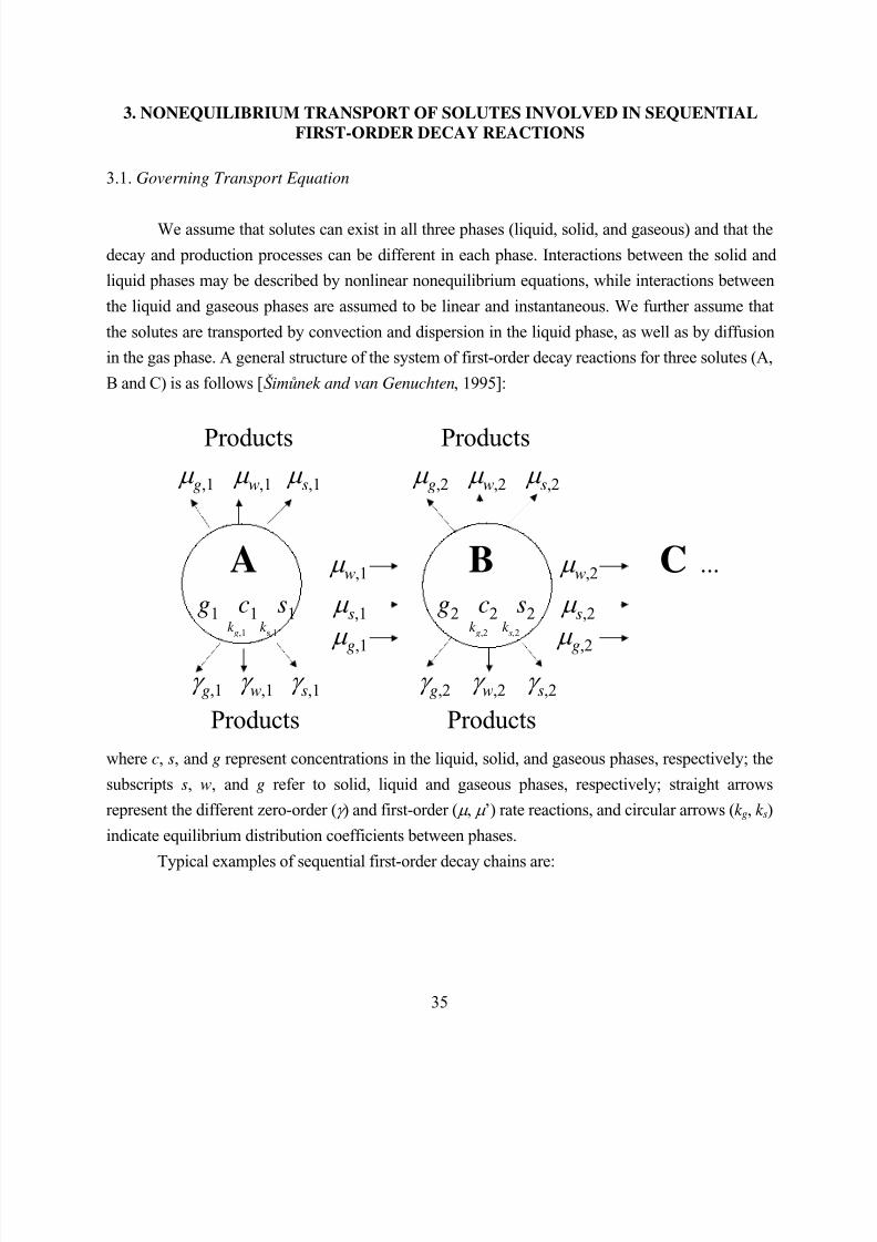
8/20/2019 HYDRUS3D Technical Manual.pdf
http://slidepdf.com/reader/full/hydrus3d-technical-manualpdf 65/260
35
3. NONEQUILIBRIUM TRANSPORT OF SOLUTES INVOLVED IN SEQUENTIAL
FIRST-ORDER DECAY REACTIONS
3.1. Governing Transport Equation
We assume that solutes can exist in all three phases (liquid, solid, and gaseous) and that the
decay and production processes can be different in each phase. Interactions between the solid and
liquid phases may be described by nonlinear nonequilibrium equations, while interactions between
the liquid and gaseous phases are assumed to be linear and instantaneous. We further assume that
the solutes are transported by convection and dispersion in the liquid phase, as well as by diffusion
in the gas phase. A general structure of the system of first-order decay reactions for three solutes (A,
B and C) is as follows [Šimůnek and van Genuchten, 1995]:
Products Products µ g,1 µ w,1 µ s,1 µ g,2 µ w,2 µ s,2
A µ w,1 B µ w,2 C ...
g1 c1 s1 µ s,1 g2 c2 s2 µ s,2 k g,1 k s,1 k g,2 k s,2 µ
g,1
µ g,2
γ g,1 γ w,1 γ s,1 γ g,2 γ w,2 γ s,2
Products Products
where c, s, and g represent concentrations in the liquid, solid, and gaseous phases, respectively; the
subscripts s, w, and g refer to solid, liquid and gaseous phases, respectively; straight arrows
represent the different zero-order (γ ) and first-order (µ , µ ’) rate reactions, and circular arrows (k g, k s)
indicate equilibrium distribution coefficients between phases.
Typical examples of sequential first-order decay chains are:
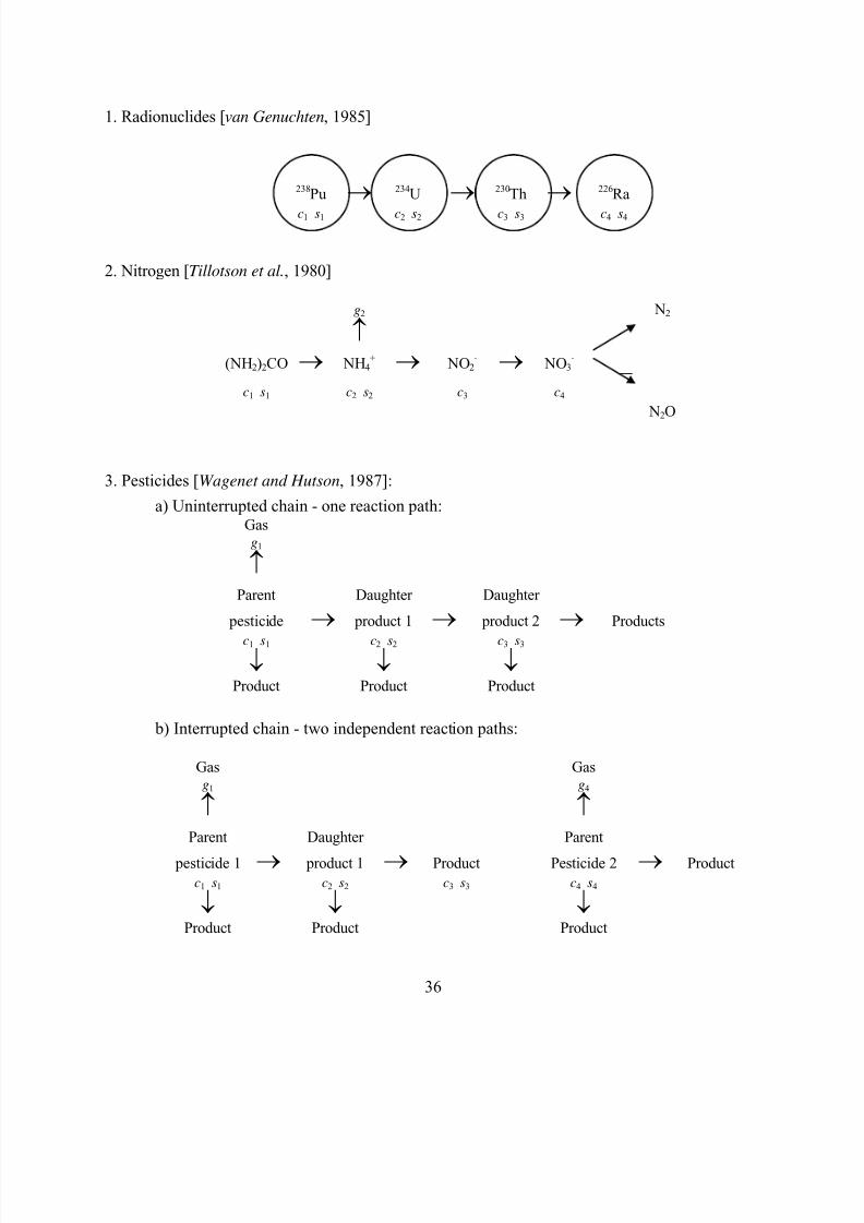
8/20/2019 HYDRUS3D Technical Manual.pdf
http://slidepdf.com/reader/full/hydrus3d-technical-manualpdf 66/260
36
1. Radionuclides [van Genuchten, 1985]
238Pu → 234U → 230Th → 226Ra
c1 s1 c2 s2 c3 s3 c4 s4
2. Nitrogen [Tillotson et al., 1980]
g2 N2
↑ (NH2)2CO → NH4
+ → NO2- → NO3
-
c1 s1 c2 s2 c3 c4 N2O
3. Pesticides [Wagenet and Hutson, 1987]:
a) Uninterrupted chain - one reaction path:Gasg1
↑ Parent Daughter Daughter
pesticide → product 1 → product 2 → Products
c1 s1 c2 s2 c3 s3 ↓ ↓ ↓
Product Product Product
b) Interrupted chain - two independent reaction paths:
Gas Gasg1 g4
↑ ↑ Parent Daughter Parent
pesticide 1 → product 1 → Product Pesticide 2 → Productc1 s1 c2 s2 c3 s3 c4 s4
↓ ↓ ↓ Product Product Product
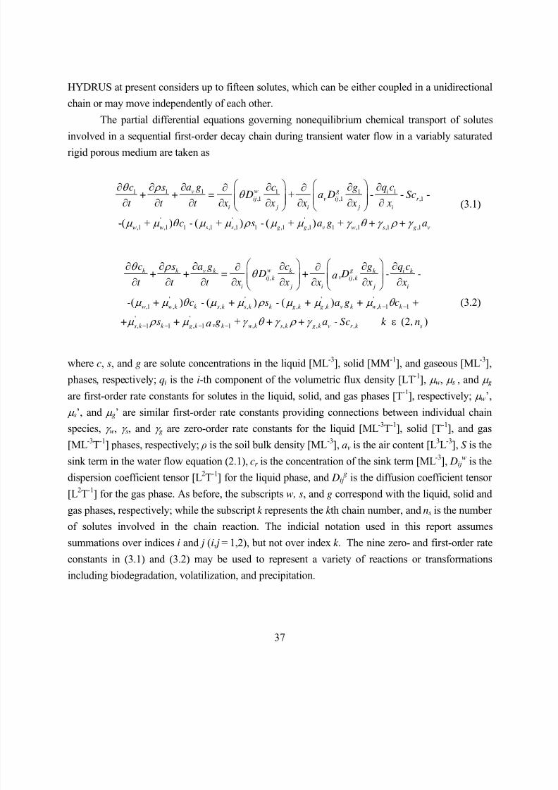
8/20/2019 HYDRUS3D Technical Manual.pdf
http://slidepdf.com/reader/full/hydrus3d-technical-manualpdf 67/260
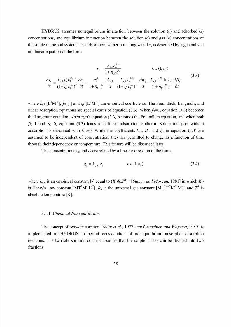
8/20/2019 HYDRUS3D Technical Manual.pdf
http://slidepdf.com/reader/full/hydrus3d-technical-manualpdf 68/260
38
HYDRUS assumes nonequilibrium interaction between the solution (c) and adsorbed (s)
concentrations, and equilibrium interaction between the solution (c) and gas (g) concentrations of
the solute in the soil system. The adsorption isotherm relating sk and ck is described by a generalized
nonlinear equation of the form
,
1 2, , , ,
2 2
(1, )1
ln-
1(1 (1 () )
k
k
k k k k
k k k
s k k
k s
k k
s k k k s k s k k s k k k k k k k
k k k k k k
k c s k n
c
k c k k c k c cs c c
t t c t t c c
β
β
β β β β
β β β
η
β η
η η η
−
= ∈+
∂ ∂∂ ∂= + +
∂ ∂ + ∂ ∂+ + 21 )k
k
k k t c
β
β
η
∂
∂+
(3.3)
where k s,k [L3M-1], β k [-] and ηk [L
3M-1] are empirical coefficients. The Freundlich, Langmuir, and
linear adsorption equations are special cases of equation (3.3). When β k =1, equation (3.3) becomes
the Langmuir equation, when η k =0, equation (3.3) becomes the Freundlich equation, and when both
β k =1 and η k =0, equation (3.3) leads to a linear adsorption isotherm. Solute transport without
adsorption is described with k s,k =0. While the coefficients k s,k , β k , and η k in equation (3.3) are
assumed to be independent of concentration, they are permitted to change as a function of time
through their dependency on temperature. This feature will be discussed later.
The concentrations gk and ck are related by a linear expression of the form
, (1, )k g k k sg = k c k n∈ (3.4)
where k g,k is an empirical constant [-] equal to (K H RuT A)-1 [Stumm and Morgan, 1981] in which K H
is Henry's Law constant [MT2M-1L-2], Ru is the universal gas constant [ML2T-2K -1 M-1] and T A is
absolute temperature [K].
3.1.1. Chemical Nonequilibrium
The concept of two-site sorption [Selim et al.
, 1977;van Genuchten and Wagenet
, 1989] isimplemented in HYDRUS to permit consideration of nonequilibrium adsorption-desorption
reactions. The two-site sorption concept assumes that the sorption sites can be divided into two
fractions:
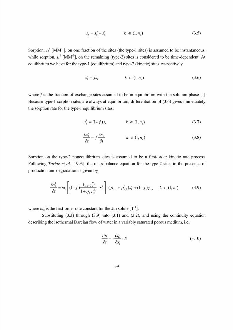
8/20/2019 HYDRUS3D Technical Manual.pdf
http://slidepdf.com/reader/full/hydrus3d-technical-manualpdf 69/260
39
(1, )e k
k k k ss s s k n= + ∈ (3.5)
Sorption, sk e [MM-1], on one fraction of the sites (the type-1 sites) is assumed to be instantaneous,
while sorption, sk k
[MM-1
], on the remaining (type-2) sites is considered to be time-dependent. Atequilibrium we have for the type-1 (equilibrium) and type-2 (kinetic) sites, respectively
(1, )e
k k ss fs k n= ∈ (3.6)
where f is the fraction of exchange sites assumed to be in equilibrium with the solution phase [-].
Because type-1 sorption sites are always at equilibrium, differentiation of (3.6) gives immediately
the sorption rate for the type-1 equilibrium sites:
(1- ) (1, )k
k k ss f s k n= ∈ (3.7)
(1, )ek k
s
s s f k n
t t
∂ ∂= ∈
∂ ∂ (3.8)
Sorption on the type-2 nonequilibrium sites is assumed to be a first-order kinetic rate process.
Following Toride et al. [1993], the mass balance equation for the type-2 sites in the presence of
production and degradation is given by
, ', ,,(1- ) - - ( ) (1- ) (1, )
1
k
k
k s k k k k k
k k s k k s k ss k
k k
s k c f s s f k n
t c
β
β ω µ γ µ
η
∂= + + ∈
∂ + (3.9)
where ωk is the first-order rate constant for the k th solute [T-1].
Substituting (3.3) through (3.9) into (3.1) and (3.2), and using the continuity equation
describing the isothermal Darcian flow of water in a variably saturated porous medium, i.e.,
i
i
q= - - S
t x
θ ∂∂
∂ ∂ (3.10)
8/20/2019 HYDRUS3D Technical Manual.pdf
http://slidepdf.com/reader/full/hydrus3d-technical-manualpdf 70/260
40
leads to the following equation
, 0 (1, )k k k
k i ij k k k k s
i i j
c c c
- R - q + D + F c +G = k nt x x xθ θ
∂ ∂ ∂∂∈ ∂ ∂ ∂ ∂ (3.11)
in which Dij [L2T-1] is an effective dispersion coefficient tensor given by
, , , , (1, )w g
ij k ij k v ij k g k s D = D +a D k k nθ θ ∈ (3.12)
The coefficients F k and Gk in (3.11) are defined as
1,' ' '
, , , , , , ,
1, ,
,
( ) ( ) ( ) ( )1
(1 )( ) (1, )
1
k
k
k
k
s k k
k k w k w k s k s k g k g k v g k
k k
g k s k k
g k v k k k s
k k
k cF c = - + - + f - + a k +
+ c
k - f k c+S +k - a - g c k n
t t + c
β
β
β
β
µ µ θ µ µ ρ µ µ η
θ ω ρ
η
−
−∂∂− ∈
∂ ∂
(3.13)
1
1
1 1 ,1 ,1 ,1 ,1 1 1
1, 1 1' ' '
, 1 , 1 , 1 , 1 1
11
', 1 1 , , , ,
( ) - +
( ) ( + ) +
1++ (2 )
k
k
k
w s g v r
s k k
k k w k s k g k v g k k
k k -
k k
s k k w k s k g k v r k k k s
G c = + f + a Sc s
k cG c = + f a k c
cs + + f + a - Sc + s k ,n
β
β
γ θ γ ρ γ ω ρ
µ θ µ ρ µ
η µ ρ γ θ γ ρ γ ω ρ
−
−
−− −
− − − − −
−
− − ∈
(3.14)
where the variable gk accounts for possible changes in the adsorption parameters caused by
temperature changes in the system as follows (see also section 3.4):
2 1 11, , ,
2 2
ln( ) - (1 )
1 (1 (1) )
k k k
k k k
s k s k s k k k k k k k k k s
k k k k k k
c c cc k k k g c f k ,n
c t t t c c
β β β
β β β
η β ρ
η η η
− −− ∂ ∂ ∂= + ∈
+ ∂ ∂ ∂+ + (3.15)
The retardation factor Rk [-] in (3.11) is given by
8/20/2019 HYDRUS3D Technical Manual.pdf
http://slidepdf.com/reader/full/hydrus3d-technical-manualpdf 71/260
41
1,,
2( ) 1 (1, )
(1 )
k
k
v g k s k k k
k k s
k k
a k fk c R c + k n
c
β
β
β ρ
θ θ η
−
= + ∈+
(3.16)
3.1.2. Physical Nonequilibrium
The concept of two-region, dual-porosity type solute transport [van Genuchten and
Wierenga, 1976] is implemented in HYDRUS to permit consideration of physical nonequilibrium
transport. The two-region concept assumes that the liquid phase can be partitioned into mobile
(flowing), θ m [L3L-3], and immobile (stagnant), θ im [L3L-3], regions:
m im= +θ θ θ (3.17)
and that solute exchange between the two liquid regions can be modeled as a first-order process,
i.e.,
1, , ,
, , ,2
,
1, ,' '
, , , , ,,
(1- ) ( - ) (1- ) -(1 )
- ( ) ( )(1- ) (1, )
k
k
k
k
s k k k im k im
im k k k im w k im s k
k k im
s k k im
im w k w k s k s k k im s
k k im
k c c f c c f
t c
k c
f c k nc
β
β
β
β
β θ ρ ω γ θ ργ
η
θ µ µ ρ µ µ η
−
−
∂+ = + +
∂+
+ + + ∈
(3.18)
where cim [ML-3] is the concentration in the immobile region and ωk is the mass transfer coefficient
for the k th solute [T-1].
Substituting (3.17) and (3.18) into (3.1) and (3.2), the latter two equations modified for
mobile and immobile regions as shown by van Genuchten and Wagenet [1989], leads to equation
(3.11) in which θ is replaced with θ m and with the coefficients F k and Gk redefined as follows
1,' ' '
, , , , , , ,( ) ( ) ( ) ( )1
k
k
s k k
k k w k w k m s k s k g k g k v g k k
k k
k cF c = - + - + f - + a k -
+ c
β
β µ µ θ µ µ ρ µ µ ω
η
−
(3.19)
8/20/2019 HYDRUS3D Technical Manual.pdf
http://slidepdf.com/reader/full/hydrus3d-technical-manualpdf 72/260
42
1
1
1
1
1 1 ,1 ,1 ,1 ,1 1 1. 1 1
1, 1 1' ' '
, 1 , 1 , 1 , 1 1
1 1
1, 1 1,' '
, 1 , 1 1.1 1,
( ) - + - ( )
( ) [ + ] +1
[ (1- ) ]1
k
k
k
k
w m s g v r im
s k k
k k w k m s k g k v g k k
k k
s k k im
w k im s k k k k im
G c = + f + a Sc c fg c
k cG c = + f a k c
c
k c
+ f cc
β
β
β
β
γ θ γ ρ γ ω ρ
µ θ µ ρ µ η
µ θ µ ρ η
−
−
−
−
−− −
− − − − −
− −
−− −
− − −− −
+
+ +
, , , , .
+
( ) (2 )
im
w k m s k g k v r k k k im k k s+ f + a - Sc + c - fg c k ,nγ θ γ ρ γ ω ρ + ∈
(3.20)
In order to solve equation (3.11), it is necessary to know the water content θ and the
volumetric flux q. Both variables are obtained from solutions of the Richards' equation. The above
equations may appear to be relatively complicated. However, by selecting proper values of
particular coefficients (i.e., γ w , γ s , γ g, µ w, µ s, µ g, µ w’, µ s’, µ g’, η , k s, k g, f , β , ω ) the entire system can
be simplified significantly. Assuming for example that µ w’, µ s’, µ g’, η , and k g are zero, and f and β
are equal to one, the entire system of equations (3.1) through (3.20) simplifies into a set of
equations describing the transport of mutually independent solutes, i.e., single-ion transport as
applicable to:
w i
ij
i j i
q cc c R = D - + Fc+G
t x x xθ θ
∂∂ ∂ ∂ ∂ ∂ ∂ ∂
(3.21)
3.1.3. Attachment-Detachment Model
Virus, colloid, and bacteria transport and fate models commonly employ a modified form
of the convection-dispersion equation. In this study we define the mass balance equation for
these applications as:
1 21 2- - ( )we i
ij ew s
i j i
s q cs sc c D - c s s s
t t t t x x x
θ ρ ρ ρ θ θ ρ µ µ
∂ ∂∂ ∂∂ ∂ ∂+ + + = + + ∂ ∂ ∂ ∂ ∂ ∂ ∂
(3.22)
where c is the (colloid, virus, bacteria) concentration in the aqueous phase [NcL-3], s is the solid phase (colloid, virus, bacteria) concentration [NcM
-1], subscripts e, 1, and 2 represent equilibrium
and two kinetic sorption sites, respectively, Nc is a number of colloids (particles), and µ w and µ s
8/20/2019 HYDRUS3D Technical Manual.pdf
http://slidepdf.com/reader/full/hydrus3d-technical-manualpdf 73/260
43
represent inactivation and degradation processes in the liquid and solid phases, respectively.
While sorption to equilibrium sites can be described similarly as before using (3.3), mass
transfer between the aqueous and both solid kinetic phases can be described as (note that we now
dropped subscripts 1 and 2):
a d
sk c k s
t ρ θ ψ ρ
∂= −
∂ (3.23)
where k a is the first-order deposition (attachment) coefficient [T-1], k d is the first-order
entrainment (detachment) coefficient [T-1], and ψ is a dimensionless colloid retention function [-
]. The attachment and detachment coefficients in (3.23) have been found to strongly depend upon
water content, with attachment significantly increasing as the water content decreases.
To simulate reductions in the attachment coefficient due to filling of favorable sorption
sites, ψ is sometimes assumed to decrease with increasing colloid mass retention. A Langmuirian
dynamics [ Adamczyk et al., 1994] equation has been proposed for ψ to describe this blocking
phenomenon:
max
max max
1s s s
s sψ
−= = − (3.24)
in which smax is the maximum solid phase concentration [NcM-1]. Blocking coefficients listed
below are implemented only into a two-dimensional formulation. Conversely, enhanced colloidretention during porous medium ripening can theoretically be described using a functional form
of ψ that increases with increasing mass of retained colloids:
( )maxmax 1, ssψ = (3.25)
Johnson and Elimelech [1995] proposed the so-called random sequential adsorption
model to describe blocking of the sorption sites:
8/20/2019 HYDRUS3D Technical Manual.pdf
http://slidepdf.com/reader/full/hydrus3d-technical-manualpdf 74/260
44
( )
2 3max
3
max2 3
max
max
1 4 3.308 1.4069 for 0.8
1for 0.8
2
1
0.546
c
a a a s s
bss s
d b
bs
sa
s
ψ
ψ
= − + + <
−= >
=
=
(3.26)
Finally, Bradford et al. [2003] hypothesized that the influence of straining and attachment
processes on colloid retention can be separated into two distinct components. They suggested the
following depth-dependent blocking coefficient for the straining process:
0c
c
d z zd
β
ψ
−
+ −=
(3.27)
where d c is the diameter of the sand grains [L], z0 is the coordinate of the location where the
straining process starts [L] (the surface of the soil profile, or interface between soil layers), and β
is an empirical factor (with an optimal value of 0.43 [ Bradford et al., 2003]) [-].
The attachment coefficient is often calculated using filtration theory [ Logan et al., 1995],
a quasi-empirical formulation in terms of the median grain diameter of the porous medium (often
termed the collector), the pore-water velocity, and collector and collision (or sticking)
efficiencies accounting for colloid removal due to diffusion, interception and gravitational
sedimentation [ Rajagopalan and Tien, 1976; Logan et al., 1995]:
3(1 )
2a
c
k vd
θ ηα
−= (3.28)
where d c is the diameter of the sand grains [L], α is the sticking efficiency (ratio of the rate of
particles that stick to a collector to the rate they strike the collector) [-], v is the pore water
velocity [LT-1
], and η is the single-collector efficiency [-]:
1/ 3 2/ 3 1/8 15/8 1.2 0.44 0.00338s Pe s Lo R s G R A N A N N A N N η − −= + + (3.29)
8/20/2019 HYDRUS3D Technical Manual.pdf
http://slidepdf.com/reader/full/hydrus3d-technical-manualpdf 75/260
45
where the first, second, and third terms represent removal by diffusion, interception, and
gravitational sedimentation, respectively, and where N Pe is the Peclet number [-], N R is the
interception number [-], N G is the gravitation number [-], N Lo accounts for the contribution of
particle London-van der Walls attractive forces to particle removal [-], and As is a correctionfactor [-] as follows:
( )
( )
5
5 6
1/ 3
2 1
2 3 3 2
1
s A
γ
γ γ γ
γ θ
−=
− + −
= −
(3.30)
The dimensionless Peclet number in (3.29) is calculated as follows:
3 p c
Pe
d d q N
kT
π µ = (3.31)
where µ is the fluid viscosity (= 0.00093 Pa s) [ML-1T-1], d p is the diameter of the particle (e.g.,
virus, bacteria) (= 0.95 µm = 0.95e-6 m) [L], q is the Darcy’s flux [LT-1], k is the Boltzman
constant (= 1.38048e-23 J/K) [M L2T-2K -1], and T is the temperature (= 298 K) [K]. Finally, the
interception number, N R, the gravitation number, N G, and the number representing London-van
der Walls attractive forces, N Lo, in (3.29) are calculated using:
p
Rc
d N
d = (3.32)
( ) 2
18
p f p
G
g d N
q
ρ ρ
µ
−= (3.33)
2
4
9 Lo
p
H N
d qπ µ = (3.34)
where H is the Hamaker constant (= 1e-20 J) [ML2T-2], g is the gravitational acceleration (= 9.81m s-2) [LT-2], ρ p is the bacterial density (= 1080 kg m-3) [ML-3], and ρ f is the fluid density (= 998
kg m-3) [ML-3].
8/20/2019 HYDRUS3D Technical Manual.pdf
http://slidepdf.com/reader/full/hydrus3d-technical-manualpdf 76/260
46
The model described above using equation (3.22) can be used in many different ways. For
example, one can assume that the soil has two sorption sites, s1 and s2, each having their own
attachment and detachment constants. This model has been used to describe virus transport in
sand dunes by Schijven and Šimůnek [2002]. Sorption sites s1 and s2 can be used to describe
straining and attachment, respectively, as was done by Bradford et al. [2002, 2003, 2004]. Onemay also assume that one sorption site represents sorption to the solid phase, while the other site
represents removal of particles by means of attachment to the air-water interface.
3.2. Initial and Boundary Conditions
The solution of (3.11) requires knowledge of the initial concentration within the flow
region, Ω , i.e.,
,
( , , , 0) ( , , )
( , , 0) ( , , )
( , , 0) ( , , )
i
k k i
im im i
c x y z = c x y z
s x y z = s x y z
c x y z = c x y z
(3.35)
where ci [ML-3], cim,i [ML-3] and sik [-] are prescribed functions of x and z. The initial condition for
sik must be specified only when nonequilibrium adsorption is considered. The subscript k is dropped
in (3.35) and throughout the remainder of this report, thus assuming that the transport-related
equations in the theoretical development and numerical solution apply to each of the solutes in the
decay chain.
Solute transport initial conditions can be alternatively specified in terms of the total
concentration S [ML-3; mass of solute/volume of soil] instead of the liquid concentration c [ML-3;
mass of solute/volume of water] as in (3.35). The liquid phase concentration is then calculated
for linear sorption as follows:
( )v s v g s v g
s v g
S c s a g c k c a k c c k a k
S ck a k
θ ρ θ ρ θ ρ
θ ρ
= + + = + + = + +
=+ +
(3.36)
and for nonlinear sorption by finding a root of the following nonlinear equation:
8/20/2019 HYDRUS3D Technical Manual.pdf
http://slidepdf.com/reader/full/hydrus3d-technical-manualpdf 77/260
47
1s
v v g
k cS c s a g c a k c
c
β
β
ρ θ ρ θ
η = + + = + +
+ (3.37)
For the two kinetic sorption sites model (only a linear case is implemented, i.e., without
blocking) the distribution coefficient k s for (3.35) is assumed to be defined as:
as
d
k k
k
θ
ρ = (3.38)
Rather than specifying directly concentrations in the nonequilibrium phases in (3.35), the
nonequilibrium phase concentration can be specified to be initially at equilibrium with
equilibrium phase concentration. In such case, the immobile water content concentration will be
set equal to the mobile water content concentration for the dual porosity models. The sorbed
concentration at the kinetic sorption sites will be set equal to:
(1 ) ss f k c= − (3.39)
for the linear sorption and:
(1 )1
sk cs f
c
β
β
ρ
η = −
+ (3.40)
for the nonlinear sorption. For the two kinetic sorption sites model, the sorbed concentrations are
set equal to:
a
d
k s c
k
θ
ρ = (3.41)
where k a and k d are the attachment and detachment coefficients, respectively.
Two types of boundary conditions (Dirichlet and Cauchy type conditions) can be specified
8/20/2019 HYDRUS3D Technical Manual.pdf
http://slidepdf.com/reader/full/hydrus3d-technical-manualpdf 78/260
48
along the boundary of Ω . First-type (or Dirichlet type) boundary conditions prescribe the
concentration along a boundary segment Γ D:
0( , , , ) ( , , , ) for ( , , ) Dc x y z t = c x y z t x y z ∈ Γ (3.42)
whereas third-type (Cauchy type) boundary conditions may be used to prescribe the concentration
flux along a boundary segment Γ C as follows:
0 for ( , , ) C ij i i i i i
j
c- D n +q n c = q n c x y z
xθ
∂∈ Γ
∂ (3.43)
in which qi ni represents the outward fluid flux, ni is the outward unit normal vector and c0 is theconcentration of the incoming fluid [ML-3]. In some cases, for example when Γ C is an impermeable
boundary (qini=0) or when water flow is directed out of the region, (3.43) reduces to a second-type
(Neumann type) boundary condition of the form:
0 for ( , , ) N ij i
j
c D n = x y z
xθ
∂∈ Γ
∂ (3.44)
A different type of boundary condition is needed for volatile solutes when they are presentin both the liquid and gas phases. This situation requires a third-type boundary condition which has
on the right-hand side an additional term to account for gas diffusion through a stagnant boundary
layer of thickness d [L] on the soil surface. The additional solute flux is proportional to the
difference in gas concentrations above and below this boundary layer [ Jury et al., 1983]. This
modified boundary condition has the form
0 ( ) for ( , , )g
C ij i i i i i g atm
j
Dc- D n +q n c = q n c + k c - g x y z
x d θ
∂∈ Γ
∂ (3.45)
where Dg is the molecular diffusion coefficient in the gas phase [L2T-1] and gatm is the gas
concentration above the stagnant boundary layer [ML-3]. We note that Jury et al. [1983] assumed
8/20/2019 HYDRUS3D Technical Manual.pdf
http://slidepdf.com/reader/full/hydrus3d-technical-manualpdf 79/260
49
gatm to be zero. Similarly as for (3.43), (3.45) reduces to a second-type (Neumann type) boundary
condition when water flow is zero or directed out of the region:
( ) for ( , , )g
N ij i g atm
j
Dc- D n = k c - g x y z
x d θ
∂∈
Γ∂ (3.46)
Equations (3.45) and (3.46) can only be used when the additional gas diffusion flux is positive.
Jury et al. [1983] discussed how to estimate the thickness of the boundary layer, d , and
recommended d =0.5 cm as a good average value for a bare surface.
3.3. Effective Dispersion Coefficient
The components of the dispersion tensor in the liquid phase, Dijw, are given by [ Bear ,
1972]
( ) j iw
ij T ij L T w w ij
q q D = D | q | + D - D + D
| q |θ δ θ τ δ (3.47)
where Dw is the molecular diffusion coefficient in free water [L2T-1], τ w is a tortuosity factor in the
liquid phase [-], |q| is the absolute value of the Darcian fluid flux density [LT-1
], δ ij is the Kroneckerdelta function (δij=1 if i=j, and δij=0 if i≠ j), and D L and DT are the longitudinal and transverse
dispersivities, respectively [L]. After adding the diffusion contribution from the gas phase, the
individual components of the effective dispersion tensor in the soil matrix for three-dimensional
transport are as follows:
8/20/2019 HYDRUS3D Technical Manual.pdf
http://slidepdf.com/reader/full/hydrus3d-technical-manualpdf 80/260
8/20/2019 HYDRUS3D Technical Manual.pdf
http://slidepdf.com/reader/full/hydrus3d-technical-manualpdf 81/260
51
relationship for calculating the tortuosity coefficient in the liquid phase:
8 / 3
0.66w
s
= θ
τ θ
(3.51)
The Millington-Quirk [1961] tortuosity models are expected to perform well for sands (since they
were derived assuming randomly distributed particles of equal size) while Modrup’s tortuosity
models are expected to perform better across soil types.
3.4. Temperature and Water Content Dependence of Transport and Reaction Coefficients
Several of the diffusion ( Dw, Dg), zero-order production (γ w, γ s, γ g ), first-order degradation(µ w’, µ s’, µ g’, µ w, µ s, and µ g), and adsorption (k s, k g, β , η , ω ) coefficients may be strongly
dependent upon temperature. HYDRUS assumes that this dependency can be expressed by the
Arrhenius equation [Stumm and Morgan, 1981]. After some modification, this equation can be
expressed in the general form
( - )exp
A Aa r
T r A Au r
E T T a = a R T T
(3.52)
where ar and aT are the values of the coefficient being considered at a reference absolute
temperature T r A and absolute temperature T A, respectively; Ru is the universal gas constant, and E a
[ML2T-2M-1] is the activation energy of the particular reaction or process being modeled.
The water content dependence of degradation coefficients is implemented using a
modified equation of Walker [1974]:
( ) ( ) min 1,
B
r r r
θ µ θ µ θ
θ
=
(3.53)
where µ r is the values of a particular coefficient (rate constant) at the reference water content θ r ,
8/20/2019 HYDRUS3D Technical Manual.pdf
http://slidepdf.com/reader/full/hydrus3d-technical-manualpdf 82/260
52
µ is the value at the actual water content θ , and B is a solute dependent parameter (usually 0.7).
The reference water content, θ r , which may be different for different soil layers, is calculated
from the reference pressure head, hr , which is considered to be constant for a particular
compound.
3.5. Root Solute Uptake
The root solute uptake models implemented in HYDRUS-1D was developed by Šimůnek
and Hopmans [2009] and only a brief description is given below.
3.5.1. Uncompensated Nutrient Uptake Model
To clearly differentiate between point and root domain nutrient uptake rate values, wedefine lower case variables to represent point root nutrient uptake rates [ML-3T-1], while upper case
variables represent nutrient uptake rates [ML-2T-1] over the entire root zone, LR . Both point and root
domain nutrient uptakes are assumed to be the sum of their passive and active components, or:
( , ) ( , ) ( , )a a ar x t p x t a x t = + (3.54)
( ) ( ) ( )a a a R t P t A t = + (3.55)
where r a, pa, and aa define total actual (subscript a) passive and active root nutrient uptake rates
[ML-3T-1], respectively, at any point, and Ra, Pa, and Aa denote actual total, passive and active root
nutrient uptake rates [ML-2T-1], respectively, for the root zone domain.
Passive nutrient uptake is simulated by multiplying root water uptake (compensated or
uncompensated) with the dissolved nutrient concentration, for concentration values below a
priori defined maximum concentration (cmax), or
[ ]*max( , ) ( , )min ( , ),a
p x t s x t c x t c= (3.56)
where c is the dissolved nutrient concentration [ML-3] and cmax is the maximum allowed solution
concentration [ML-3] that can be taken up by plant roots during passive root uptake. All nutrient
8/20/2019 HYDRUS3D Technical Manual.pdf
http://slidepdf.com/reader/full/hydrus3d-technical-manualpdf 83/260
53
dissolved in water is taken up by plant roots when cmax is large (larger than the dissolved
concentration c), while no nutrient is taken up when cmax is equal to zero, with only active uptake
remaining in that case. The maximum solution concentration for passive root uptake, cmax, thus
controls the relative proportion of passive root water uptake to total uptake. Using this flexible
formulation, uptake mechanisms can vary between specific nutrients. For example, Na uptake can be excluded by setting cmax equal to zero, passive Ca uptake can be limited by defining a finite cmax
value, or all soil solution available P or N is allowed to be taken up passively, by setting cmax to a
very large value. Note that the cmax parameter is introduced as a control model parameter that
does not necessarily have a physiological meaning.
Passive actual root nutrient uptake for the whole root domain, Pa [ML-2T-1], is calculated by
integrating the local passive root nutrient uptake rate, pa, over the entire root zone:
[ ]
[ ] [ ]
*max
max
( ) ( , ) ( , ) min ( , ),
( )( , , ) ( , ) min ( , ),
max ( ),
R R
R
a a
L L
p
c
P t p x t dx s x t c x t c dx
T t h,h x t b x t c x t c dx
t φ α
ω ω Ω
= = =
=
∫ ∫
∫ (3.57)
Defining R p as the potential (subscript p) nutrient demand [ML-2T-1], the potential active nutrient
uptake rate, A p [ML-2T-1], is computed from:
( ) max ( ) ( ),0 p p a A t R t P t = − (3.58)
Thus, using this formulation, we assume that active nutrient uptake will be invoked only if the
passive root nutrient uptake term does not fully satisfy the potential nutrient demand of the plant.
However, as was discussed earlier, the passive uptake can be reduced or completely turned off
(cmax=0), thus allowing the potential active nutrient uptake ( A p) to be equal to the potential nutrient
demand ( R p). Once A p is known, the point values of potential active nutrient uptake rates, a p [ML-
3T-1], are obtained by distributing the potential root zone active nutrient uptake rate, A p [ML-2T-1],
over the root zone, using a predefined spatial root distribution, b( x, t ), as was done for root wateruptake, or:
8/20/2019 HYDRUS3D Technical Manual.pdf
http://slidepdf.com/reader/full/hydrus3d-technical-manualpdf 84/260
54
( , ) ( , ) ( ) p t pa x t b x t L A t = (3.59)
Using Michaelis-Menten kinetics (e.g., Jungk [1991]) provides for actual distributed values of
active nutrient uptake rates, aa [ML-3
T-1
], allowing for nutrient concentration dependency, or:
( , , ) ( , , )( , , ) ( , , ) ( , , ) ( )
( , , ) ( , , )a p t p
m m
c x z t c x z t a x z t a x z t b x z t L A t
K c x z t K c x z t = =
+ + (3.60)
where K m is the Michaelis-Menten constant [ML-3] [ Jungk , 1991]. The Michaelis-Menten
constants for selected nutrients (e.g., N, P, and K) and plant species (e.g., corn, soybean, wheat,
tomato, pepper, lettuce, and barley) can be found in the literature (e.g., Bar-Yosef [1999]).
Finally, total active uncompensated root nutrient uptake rate, Aa [ML-2T-1], is calculated byintegrating the actual active root nutrient uptake rate, aa, at each point, over the root zone L R, in
analogy with the non-compensated root water uptake term, or:
( , )( ) ( , ) ( ) ( , )
( , ) R R
a a p
m L L
c x t A t a x t dx A t b x t dx
K c x t = =
+∫ ∫ (3.61)
3.5.2. Compensated Nutrient Uptake Model
The above nutrient uptake model includes compensation of the passive nutrient uptake, by
way of the root water uptake compensation term, sc , and root adaptability factor, ω c, in Eq. (3.57).
A similar compensation concept as used for root water uptake above, was implemented for active
nutrient uptake rate, by invoking a so-called nutrient stress index π :
( )( )
( )a
p
A t t
A t π = (3.62)
After substitution of the active total root nutrient uptake rate value from Eq. (3.61) above, this
newly defined nutrient stress index (π ) is equal to:
8/20/2019 HYDRUS3D Technical Manual.pdf
http://slidepdf.com/reader/full/hydrus3d-technical-manualpdf 85/260
55
( , )( ) ( , )
( , ) R m L
c x t t b x t dx
K c x t π =
+∫ (3.63)
After defining the critical value of the nutrient stress index π c, above which value active nutrient
uptake is fully compensated for by active uptake in other more-available (less stressed) soil
regions, the local compensated active root nutrient uptake rate, aac [ML-3T-1], is obtained by
including the nutrient-stress index function in the denominator of Eq. (3.60), or:
[ ]
( )( , )( , ) ( , )
( , ) max ( ),
p
ac
m c
A t c x t a x t b x t
K c x t t π π =
+ (3.64)
from which the total compensated active root nutrient uptake rate, Aac [ML-2T-1] in the two-
dimensional root domain, L R, is calculated, in analogy with the compensated root water uptake
term, as follows:
[ ]
( ) ( , )( ) ( , ) ( , )
max ( ), ( , ) R R
p
ac acc m L L
A t c x t A t a x t dx b x t dx
t K c x t π π = =
+∫ ∫ (3.65)
Equation (3.57) implies that reduction in root water uptake will decrease passive nutrient uptake,thereby increasing active nutrient uptake proportionally. In other words, total nutrient uptake is not
affected by soil water stress, as computed by the proportion of actual to potential root water uptake.
This is not realistic since one would expect that plant nutrient requirements will be reduced for
water-stressed plants. For that reason, the uptake model includes additional flexibility, by reducing
the potential nutrient demand R p [ML-2T-1], in proportion to the reduction of root water uptake, as
defined by the actual to potential transpiration ratio, or:
( )( ) max ( ) ( ),0( )ac
p p a
p
T t A t R t P t
T t
= − (3.66)
8/20/2019 HYDRUS3D Technical Manual.pdf
http://slidepdf.com/reader/full/hydrus3d-technical-manualpdf 86/260
8/20/2019 HYDRUS3D Technical Manual.pdf
http://slidepdf.com/reader/full/hydrus3d-technical-manualpdf 87/260
57
4. HEAT TRANSPORT
4.1. Governing Heat Transport Equations
Neglecting the effects of water vapor diffusion, two- and three-dimensional heat transportcan be described as [Sophocleous, 1979]:
( ) ( )ij w i
i j i
T T T C = - C q
t x x xθ λ θ
∂ ∂ ∂ ∂ ∂ ∂ ∂ ∂
(4.1)
where λ ij(θ ) is the apparent thermal conductivity of the soil [MLT-3K -1] (e.g. Wm-1K -1) and C (θ )
and C w are the volumetric heat capacities [ML-1T-2K -1] (e.g. Jm-3K -1) of the porous medium and the
liquid phase, respectively. Volumetric heat capacity is defined as the product of the bulk densityand gravimetric heat capacity. The first term on the right-hand side of (4.1) represents heat flow due
to conduction and the second term accounts for heat being transported by flowing water. We do not
consider the transfer of latent heat by vapor movement.According to de Vries [1963] the volumetric
heat capacity can be expressed as
6 -3 o -1( ) (1.92 2.51 4.18 )10 ( J m C ) p n n o o w g v n oC C C C C aθ θ θ θ θ θ θ = + + + ≈ + + (4.2)
where θ refers to a volumetric fraction [L3
L-3
], and subscripts n, o, g, w represent solid phase,organic matter, gas phase and liquid phase, respectively.
4.2. Apparent Thermal Conductivity Coefficient
The apparent thermal conductivity, λ ij(θ ), combines the thermal conductivity λ0(θ ) of the
porous medium (solid plus water) in the absence of flow, and the macrodispersivity which is
assumed to be a linear function of the velocity [de Marsily, 1986]. In analogy with the dispersion
coefficient for solute transport, the apparent thermal conductivity λ ij(θ ) is given by [Šimůnek andSuarez, 1993b]
8/20/2019 HYDRUS3D Technical Manual.pdf
http://slidepdf.com/reader/full/hydrus3d-technical-manualpdf 88/260
58
0( ) ( ) ( ) j i
ij T w ij L T w ij
q qC | q | + - c +
| q |λ θ λ δ λ λ λ θ δ = (4.3)
where q is the absolute value of the Darcian fluid flux density [LT
-1
], δ ij is the Kronecker deltafunction as before, and λ L and λ T are the longitudinal and transverse thermal dispersivities [L],
respectively. The individual components of the thermal conductivity tensor for three-dimensional
transport are as follows:
22 2
0
2 2 2
0
22 2
0
( )
( )
( )
y x z xx L w T w T w
y x z yy L w T w T w
y z z zz L w T w T w
x y xy L T w
x z xz L T w
y z yz L T w
x x x= C + C + C +
| q | | q | | q |
x x x= C + C + C +
| q | | q | | q |
x x x= C + C + C +
| q | | q | | q |
q q= - C
| q |
q q= - C
| q |
q q= - C
| q |
λ λ λ λ λ
λ λ λ λ λ
λ λ λ λ λ
λ λ λ
λ λ λ
λ λ λ
(4.4)
The volumetric heat capacity of the liquid phase is included here in the definition of the thermal
conductivity in order to have the dimensions of the thermal dispersivities in the length units [ de
Marsily, 1986]. The thermal conductivity, λ 0(θ ), accounts for the tortuosity of the porous medium,
and is described with the simple equation [Chung and Horton, 1987]
0.50 1 2 2( ) w w
= b +b +bλ θ θ θ (4.5)
where b1, b2 and b3 are empirical parameters [MLT-3K -1] (e.g. Wm-1K -1).
8/20/2019 HYDRUS3D Technical Manual.pdf
http://slidepdf.com/reader/full/hydrus3d-technical-manualpdf 89/260
59
4.3. Initial and Boundary Conditions
Equation (4.1) will be solved subject to the general initial condition
( , , ,0) ( , , )iT x y z = T x y z (4.6)
where T i is a prescribed function of x and z.
Two types of boundary conditions (Dirichlet and Cauchy type conditions) can again be
specified along the boundary of Ω . First-type (or Dirichlet type) boundary conditions prescribe the
temperature along a boundary segment Γ D:
0( , , , ) ( , , , ) for ( , , ) DT x y z t = T x y z t x y z ∈ Γ (4.7)
whereas third-type (Cauchy type) boundary conditions prescribe the heat flux along a boundary
segment Γ C as follows
0 for ( , , ) C ij i w i i w i i
j
T - n +Tc q n = T C q n x y z
xλ
∂∈ Γ
∂ (4.8)
in which qi ni represents the outward fluid flux, ni is the outward unit normal vector and T 0 is the
temperature of the incoming fluid. When Γ C is an impermeable boundary (qini=0) or when waterflow is directed out of the region, (4.8) reduces to a second-type (Neumann type) boundary
condition of the form:
0 for ( , , ) N ij i
j
T n = x y z
xλ
∂∈ Γ
∂ (4.9)
The atmospheric boundary condition for soil temperature is assumed to be given by a sine
function as follows [Kirkham and Powers, 1972]:
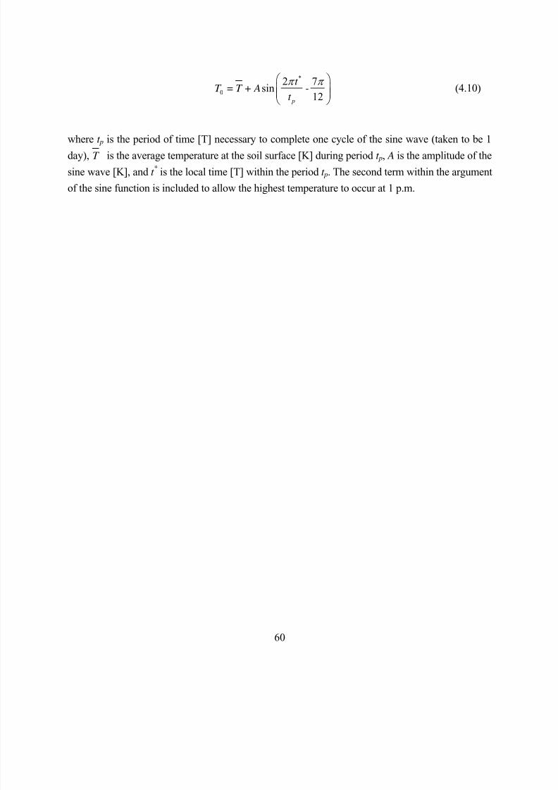
8/20/2019 HYDRUS3D Technical Manual.pdf
http://slidepdf.com/reader/full/hydrus3d-technical-manualpdf 90/260
60
*
0
2 7sin
12 p
t T = T + A -
t
π π
(4.10)
where t p is the period of time [T] necessary to complete one cycle of the sine wave (taken to be 1day), T is the average temperature at the soil surface [K] during period t p, A is the amplitude of the
sine wave [K], and t * is the local time [T] within the period t p. The second term within the argument
of the sine function is included to allow the highest temperature to occur at 1 p.m.
8/20/2019 HYDRUS3D Technical Manual.pdf
http://slidepdf.com/reader/full/hydrus3d-technical-manualpdf 91/260
61
5. NUMERICAL SOLUTION OF THE WATER FLOW EQUATION
The Galerkin finite element method with linear basis functions is used to obtain a solution
of the flow equation (2.1) subject to the imposed initial and boundary conditions. Since the
Galerkin method is relatively standard and has been covered in detail elsewhere [ Neuman, 1975; Zienkiewicz, 1977; Pinder and Gray, 1977], only the most pertinent steps in the solution process
are given here.
5.1. Space Discretization
The flow region is divided into a network of triangular (2D) or tetrahedral (3D) elements.
The corners of these elements are taken to be the nodal points. The dependent variable, the pressure
head function h( x, y, z,t ), is approximated by a function h’( x, y, z,t ) as follows
1
( , , , ) ( , , ) ( ) N
n n
n=
h’ x y z t = x y z h tφ ∑ (5.1)
where φ n are piecewise linear basis functions satisfying the condition φ n( xm ,zm)=δ nm, hn are
unknown coefficients representing the solution of (2.1) at the nodal points, and N is the total
number of nodal points.
The Galerkin method postulates that the differential operator associated with the Richards'equation (2.1) is orthogonal to each of the N basis functions, i.e.,
- 0 A A
ij iz n
i j
h K K K S d
t x x
θ φ
Ω
∂ ∂ ∂ + + Ω = ∂ ∂ ∂
∫ (5.2)
Applying Green's first identity to (5.2), and replacing h by h Ν, leads to
8/20/2019 HYDRUS3D Technical Manual.pdf
http://slidepdf.com/reader/full/hydrus3d-technical-manualpdf 92/260
62
'
'
e
e e
A n
n ij
e j i
A A A n
ij iz i n iz n
e e j i
h + KK d =
t x x
hK K + K n d + -KK - S d
x x
φ θ φ
φ φ φ
Ω
Γ Ω
∂∂ ∂Ω ∂ ∂ ∂
∂∂Γ Ω
∂ ∂
∑∫
∑ ∑∫ ∫ (5.3)
where Ω e represents the domain occupied by element e, and Γ e is a boundary segment of element e.
Natural flux-type (Neumann) and gradient type boundary conditions can be immediately
incorporated into the numerical scheme by specifying the line integral in equation (5.3).
After imposing additional simplifying assumptions to be discussed later, and performing
integration over the elements, the procedure leads to a system of time-dependent ordinary
differential equations with nonlinear coefficients. In matrix form, these equations are given by
[ ] [ ] - -
d F A h Q B D
dt
θ + = (5.4)
where
( )
( ) ( )
( ) for 2D4
[36
] for 3D
e
A n m
nm l ij l
e i j
A A A
xx m n xz m n m n zz m n
e e
A A A A xx m n yy m n zz n m xy m n m n
e e
A A
xz n m n m yz m n m n
A K K d x x
K K b b + K c b +b c + K c c A
K K b b K c c K d d K b c c bV
K b d d b K c d d c
φ φ φ
κ
Ω
∂ ∂= Ω =
∂ ∂
=
= + + + + +
+ + + +
∑ ∫
∑
∑
(5.5)
( )
( )
for 2D2
for 3D6
e
A A Ann l iz l xz n zz n
e ei
A A A xz n yz n zz n
e
B = K K d K K b + K c x
K K b K c K d
φ κ φ
Ω
∂Ω =
∂
= + +
∑ ∑∫
∑ (5.6)
8/20/2019 HYDRUS3D Technical Manual.pdf
http://slidepdf.com/reader/full/hydrus3d-technical-manualpdf 93/260
63
for 2D3
for 3D4
e
nm nm n nm e
e e
e
nm
e
F d A
V
κ δ φ δ
δ
Ω
= Ω =
=
∑ ∑∫
∑ (5.7)
1 1
e
n l l n n n
e e
Q d Lσ φ φ σ Γ
= − Γ = −∑ ∑∫ (5.8)
( )
(3 ) for 2D12
4 for 3D20
e
n l l n e ne e
en
e
D S d A S + S
V S S
κ φ φ
Ω
= Ω =
= +
∑ ∑∫
∑ (5.9)
where the overlined variables represent average values over an element e, the subscripts i and j are
space direction indices (i,j = 1,2(,3)). For a two-dimensional problem:
1,2,..., 1,2,..., 1,2,...,
2 3 3
i j k i k j
j k i j i k
k i j k j i
k j j k i j k i j K
e
l N m N n N
b = z - z c = x - x
b = z - z c = x - x
b = z - z c = x - x
c b - c b K + K + K S + S + S A = K = S =
= = =
(5.10)
For tetrahedral element vertexed by nodes 1, 2, 3, and 4 of a three-dimensional problem:
8/20/2019 HYDRUS3D Technical Manual.pdf
http://slidepdf.com/reader/full/hydrus3d-technical-manualpdf 94/260
64
( )( ) ( ) ( )
( ) ( ) ( ) ( )
( ) ( ) ( )( )
( )( ) ( ) ( )
( ) ( ) ( ) ( )
( ) ( ) ( ) ( )
( ) ( ) ( )( )
( ) ( ) ( )( )
1 4 2 3 2 3 2 4 2
2 4 3 1 3 1 3 4 3
3 2 4 1 4 1 4 2 4
4 2 1 3 1 3 1 2 1
1 3 2 4 2 4 2 3 2
2 1 3 4 3 4 3 1 3
3 1 4 2 4 2 4 1 4
4 3 1 2 1 2 1 3 1
b y y z z y y z z
b y y z z y y z z
b y y z z y y z z
b y y z z y y z z
c x x z z x x z z
c x x z z x x z z
c x x z z x x z z
c x x z z x x z z
= − − − − −
= − − − − −
= − − − − −
= − − − − −
= − − − − −
= − − − − −
= − − − − −
= − − − − −
(5.11)
( ) ( ) ( )( )
( )( ) ( ) ( )( ) ( ) ( ) ( )
( ) ( ) ( )( )
( ) ( ) ( )
1 4 2 3 2 3 2 4 2
2 4 3 1 3 1 3 4 3
3 2 4 1 4 1 4 2 4
4 2 1 3 1 3 1 2 1
4 1 4 4 1 4 4 1 4e
d x x y y x x y y
d x x y y x x y y
d x x y y x x y y
d x x y y x x y y
V x x b y y c z z d
= − − − − −
= − − − − −
= − − − − −
= − − − − −
= − + − + −
1 2 3 4 1 2 3 4
4 4
K K K K S S S S K S
+ + + + + += = (5.12)
Equation (5.8) is valid for a flux-type boundary condition. For a gradient-type boundary condition
the variable σ 1 in (5.8) must be replaced by the product of the hydraulic conductivity K and the
prescribed gradient σ 2 (=1). Equations (5.5) through (5.9) hold for flow in a three-dimensional
Cartesian ( x,y,z) domain, a two-dimensional Cartesian ( x,z) domain, as well as for flow in an
axisymmetric ( x,z) system in which x is used as the radial coordinate. For two-dimensional plane
flow we have
12
nn L= =κ λ (5.13)
8/20/2019 HYDRUS3D Technical Manual.pdf
http://slidepdf.com/reader/full/hydrus3d-technical-manualpdf 95/260
65
while for axisymmetric flow (using two-dimensional formulation)
22
3 3i j k n n
n n
x + x + x x + x’= = Lκ π λ π (5.14)
The subscripts i, j and k in equations (5.10) and (5.14) represent the three corners of a triangular
element e. Ae is the area of a two-dimensional element e, V e is the volume of a three-dimensional
element e, K and S are the average hydraulic conductivity and root water extraction values over
element e, Ln is the length of the boundary segment connected to node n, and x’n is the x-coordinate
of a boundary node adjacent to node n. The symbol σ n in equation (5.8) stands for the flux [LT-1]
across the boundary in the vicinity of boundary node n (positive when directed outward of the
system). The boundary flux is assumed to be uniform over each boundary segment. The entries of
the vector Qn are zero at all internal nodes, which do not act as sources or sinks for water.
The numerical procedure leading to (5.4) incorporates two important assumptions in
addition to those related to the Galerkin finite element approach. One assumption concerns the time
derivatives of the nodal values of the water content in (5.4). These time derivatives were weighted
according to
e
e
nen
n
e
d t d
dt d
θ φ
θ
φ
Ω
Ω
∂Ω
∂=
Ω
∑ ∫
∑ ∫ (5.15)
This assumption implements mass-lumping, which has been shown to improve the rate of
convergence of the iterative solution process [e.g., Neuman, 1973].
A second assumption in the numerical scheme is related to the anisotropy tensor K A which
is taken to be constant over each element. By contrast, the water content θ , the hydraulic
conductivity K , the soil water capacity C , and the root water extraction rate S, at a given point in
time are assumed to vary linearly over each element, e. For example, the water content is expanded
over each element as follows:
8/20/2019 HYDRUS3D Technical Manual.pdf
http://slidepdf.com/reader/full/hydrus3d-technical-manualpdf 96/260
66
( ) ( ) ( ) ( )
( ) ( ) ( ) ( )
3
1
4
1
, , , for ,
, , , , , , for , ,
n n n e
n
n n n n e
n
x z x z x z x z
x y z x y z x y z x y z
θ θ φ
θ θ φ
=
=
= ∈ Ω
= ∈ Ω
∑
∑ (5.16)
where n stands for the corners of element e. The advantage of linear interpolation is that no
numerical integration is needed to evaluate the coefficients in (5.4).
5.2. Time Discretization
Integration of (5.4) in time is achieved by discretizing the time domain into a sequence of
finite intervals and replacing the time derivatives by finite differences. An implicit (backward)finite difference scheme is used for both saturated and unsaturated conditions:
[ ]
[ ] 1
1 11
j j
j j j j j j
F A h Q B Dt
θ θ +
+ ++
−+ = − −
∆ (5.17)
where j+1 denotes the current time level at which the solution is being considered, j refers to the
previous time level, and ∆t j=t j+1-t j. Equation (5.17) represents the final set of algebraic equations to
be solved. Since the coefficients θ , A, B, D, and Q (Q for only gradient-type boundary conditions)are functions of h, the set of equations is generally highly nonlinear. Note that the vectors D and Q
are evaluated at the old time level.
5.3. Numerical Solution Strategy
5.3.1. Iterative Process
Because of the nonlinear nature of (5.17), an iterative process must be used to obtainsolutions of the global matrix equation at each new time step. For each iteration a system of
linearized algebraic equations is first derived from (5.17), which, after incorporation of the
8/20/2019 HYDRUS3D Technical Manual.pdf
http://slidepdf.com/reader/full/hydrus3d-technical-manualpdf 97/260
67
boundary conditions, is solved using either Gaussian elimination or the conjugate gradient method
(see Section 8.5). The Gaussian elimination process takes advantage of the banded and symmetric
features of the coefficient matrices in (5.17). After inversion, the coefficients in (5.17) are
re-evaluated using the first solution, and the new equations are again solved. The iterative process
continues until a satisfactory degree of convergence is obtained, i.e., until at all nodes in thesaturated (or unsaturated) region the absolute change in pressure head (or water content) between
two successive iterations becomes less than some small value determined by the imposed absolute
pressure head (or water content) tolerance [Šimůnek and van Genuchten, 1994]. The first estimate
(at zero iteration) of the unknown pressure heads at each time step is obtained by extrapolation
from the pressure head values at the previous two time levels.
5.3.2. Treatment of the Water Capacity Term
The iteration process is extremely sensitive to the method used for evaluating the water
content term (∆θ /∆t ) in equation (5.17). The present version of HYDRUS code uses the "mass-
conservative" method proposed by Celia et al. [1990]. Their method has been shown to provide
excellent results in terms of minimizing the mass balance error. The mass-conservative method
proceeds by separating the water content term into two parts:
[ ]
[ ]
[ ]
1
1 1 1 1
k k k
j j j j j j
j j jF F F t t t
θ θ θ θ θ θ +
+ + + +− − −
= +∆ ∆ ∆ (5.18)
where k +1 and k denote the current and previous iteration levels, respectively; and j+1 and j the
current and previous time levels, respectively. Notice that the second term on the right hand side of
(5.18) is known prior to the current iteration. The first term on the right hand side can be expressed
in terms of the pressure head, so that (5.18) becomes
[ ]
[ ] [ ]
[ ]
1
1 1 1 1
1
k k k
j j j j j j
j j j j
h h
F F C F t t t
θ θ θ θ +
+ + + +
+
− − −
= +∆ ∆ ∆ (5.19)
8/20/2019 HYDRUS3D Technical Manual.pdf
http://slidepdf.com/reader/full/hydrus3d-technical-manualpdf 98/260
68
where C nm=δ nmC n, in which C n represents the nodal value of the soil water capacity. The first term
on the right hand side of (5.19) should vanish at the end of the iteration process if the numerical
solution converges. This particular feature guarantees relatively small mass balance errors in the
solution.
5.3.3. Time Control
Three different time discretizations are introduced in HYDRUS: (1) time discretizations
associated with the numerical solution, (2) time discretizations associated with the implementation
of boundary conditions, and (3) time discretizations which provide printed output of the simulation
results (e.g., nodal values of dependent variables, water and solute mass balance components, and
other information about the flow regime).
Discretizations 2 and 3 are mutually independent; they generally involve variable time steps
as described in the input data file. Discretization 1 starts with a prescribed initial time increment, Δt .
This time increment is automatically adjusted at each time level according to the following rules
[ Mls, 1982; Vogel, 1987]:
a. Discretization 1 must coincide with time values resulting from discretizations 2 and 3.
b. Time increments cannot become less than a preselected minimum time step, ∆t min, nor
exceed a maximum time step, Δt max (i.e., ∆t min≤ Δt ≤∆t max).
c. If, during a particular time step, the number of iterations necessary to reach convergence
is ≤3, the time increment for the next time step i s increased by multiplying ∆t by a predetermined constant >1 (usually between 1.1 and 1.5). If the number of iterations is
≥7, Δt for the next time level is multiplied by a constant <1 (usually between 0.3 and
0.9).
d. If, during a particular time step, the number of iterations at any time level becomes
greater than a prescribed maximum (usually between 10 and 50), the iterative process
for that time level is terminated. The time step is subsequently reset to ∆t /3, and the
iterative process restarted.
The selection of optimal time steps, ∆t , is also influenced by the solution scheme for solute
transport (see Section 6.4.6).
8/20/2019 HYDRUS3D Technical Manual.pdf
http://slidepdf.com/reader/full/hydrus3d-technical-manualpdf 99/260
69
5.3.4. Treatment of Pressure Head Boundary Conditions
Finite element equations corresponding to Dirichlet nodes where the pressure head is
prescribed can, at least in principle, be eliminated from the global matrix equation. An alternative
and numerically simpler approach is to replace the Dirichlet finite element equations by dummyexpressions of the form [ Neuman, 1974]
nm m nhδ ψ = (5.20)
where δ nm is the Kronecker delta and ψ n is the prescribed value of the pressure head at node n. The
values of hn in all other equations are set equal to ψ n and the appropriate entries containing ψ n in the
left hand side matrix are incorporated into the known vector on the right-hand side of the global
matrix equation. When done properly, this rearrangement will preserve symmetry in the matrixequation. This procedure is applied only when Gaussian elimination is used to solve the matrix
equations. When the conjugate gradient solver is used, then the finite element equation representing
the Dirichlet node is modified as follows. The right hand side of this equation is set equal to the
prescribed pressure head multiplied by a large number (1030), and entry on the left hand side
representing the Dirichlet node is set equal to this large number. After solving for all pressure
heads, the value of the flux Qn can be calculated explicitly and accurately from the original finite
element equation associated with node n [e.g., Lynch, 1984].
5.3.5. Flux and Gradient Boundary Conditions
The values of the fluxes Qn at nodal points along prescribed flux and gradient boundaries
are computed according to equation (5.8). Internal nodes which act as Neumann type sources or
sinks have values of Qn equal to the imposed fluid injection or extraction rate.
5.3.6. Atmospheric Boundary Conditions and Seepage Faces
Atmospheric boundaries are simulated by applying either prescribed head or prescribed flux
boundary conditions depending upon whether equation (2.60) or (2.61) is satisfied [ Neuman, 1974].
8/20/2019 HYDRUS3D Technical Manual.pdf
http://slidepdf.com/reader/full/hydrus3d-technical-manualpdf 100/260
70
If (2.61) is not satisfied, node n becomes a prescribed head boundary. If, at any point in time during
the computations, the calculated flux exceeds the specified potential flux in (2.47), the node will be
assigned a flux equal to the potential value and treated again as a prescribed flux boundary.
All nodes expected to be part of a seepage face during code execution must be identified a
priori. During each iteration, the saturated part of a potential seepage face is treated as a prescribed pressure head boundary with h=0, while the unsaturated part is treated as a prescribed flux
boundary with Q=0. The lengths of the two surface segments are continually adjusted [ Neuman,
1974] during the iterative process until the calculated values of Q (equation (5.8)) along the
saturated part, and the calculated values of h along the unsaturated part, are all negative, thus
indicating that water is leaving the flow region through the saturated part of the surface boundary
only.
5.3.7. Tile Drains as Boundary Conditions
The representation of tile drains as boundary conditions is based on studies by Vimoke et al.
[1963] and Fipps et al. [1986]. The approach uses results of electric analog experiments conducted
by Vimoke and Taylor [1962] who reasoned that drains can be represented by nodal points in a
regular finite element mesh, provided adjustments are made in the hydraulic conductivity, K , of
neighboring elements. The adjustments should correspond to changes in the electric resistance of
conducting paper as follows
drain d K KC = (5.21)
where K drain is the adjusted conductivity [LT-1], and C d is the correction factor [-]. C d is determined
from the ratio of the effective radius, d e [L], of the drain to the side length, D [L], of the square
formed by finite elements surrounding the drain node [Vimoke at al., 1962]:
0 00
0 10
/
138log 6.48 2.34 0.48 0.12d
d
Z C
Z A B C
µ ε
ρ
′= ≈
+ − − − (5.22)
where Z 0’ is the characteristic impedance of free space (≈376.7 ohms), µ 0 is the permeability of free
8/20/2019 HYDRUS3D Technical Manual.pdf
http://slidepdf.com/reader/full/hydrus3d-technical-manualpdf 101/260
8/20/2019 HYDRUS3D Technical Manual.pdf
http://slidepdf.com/reader/full/hydrus3d-technical-manualpdf 102/260
72
for 2D3
for 3D4
i j k e
e
i j k l
ee
V A
V V
θ θ θ κ
θ θ θ θ
+ +=
+ + +=
∑
∑ (5.24)
and
new old V V O
t
−=
(5.25)
respectively, where θ i, θ j θ k , and θ l are water contents evaluated at the corner nodes of element e,
and where V new and V old are volumes of water in the subregion computed at the current and previous
time levels, respectively. The summation in (5.24) is taken over all elements within the subregion.
The absolute error in the mass balance is calculated as
0
0 0
t t
w
a t t a n
n
V V S T dt Q dt ε Γ
= − + − ∑∫ ∫ (5.26)
where V t and V 0 are the volumes of water in the flow domain at time t and zero, respectively, as
calculated with (5.24). The third term on the right-hand side represents the cumulative root water
uptake amount, while the fourth term gives the cumulative flux through nodes, nΓ , located along the
boundary of the flow domain or at internal source and sink nodes.The accuracy of the numerical solution is evaluated in terms of the relative error, ε r
w [%], in
the water mass balance as follows:
0
0 0
max ,
w
aw
r t t
e e
t t a n
e n
V V S T dt Q dt
ε ε
Γ
=
− + ∑ ∑∫ ∫
(5.27)
where V t e and V 0e are the volumes of water in element e at times t and zero, respectively. Note thatHYDRUS does not relate the absolute error to the volume of water in the flow domain, but instead
to the maximum value of two quantities. The first quantity represents the sum of the absolute
8/20/2019 HYDRUS3D Technical Manual.pdf
http://slidepdf.com/reader/full/hydrus3d-technical-manualpdf 103/260
73
changes in water content over all elements, whereas the second quantity is the sum of the absolute
values of all fluxes in and out of the flow domain. This criterion is much stricter than the usual
criterion involving the total volume of water in the flow domain. This is because cumulative
boundary fluxes are often much smaller than the volume in the domain, especially at the beginning
of the simulation.
5.3.9. Computation of Nodal Fluxes
Components of the Darcian flux are computed at each time level during the simulation only
when the water flow and solute transport equations are solved simultaneously. When the flow
equation is being solved alone, the flux components are calculated only at selected print times. The
x- and z-components of the nodal fluxes for a two-dimensional problem are computed for each node
n according to:
2
2
n
n
x x x
i i j j k k An
x xz
ee e
z z z
i i j j k k An
z zz
ee e
x A A
n xx n xz n
z A A
n xz n zz n
h h hK q K
N A
h h hK q K
N A
K b K c
K b K c
γ γ γ
γ γ γ
γ
γ
+ += − +
+ += − +
= +
= +
∑
∑ (5.28)
and x-, y- and z-components for a three-dimensional problem as follows:
8/20/2019 HYDRUS3D Technical Manual.pdf
http://slidepdf.com/reader/full/hydrus3d-technical-manualpdf 104/260
74
6
6
6
n
n
n
x x x x
i i j j k k l l An
x xz
ee e
y y y y
i i j j k k l l An
y yz
ee e
z z z z
i i j j k k l l An
z zz
ee e
x A A A
n xx n xy n xz n
y A A A
n xy n yy n yz n
n
h h h hK q K
N V
h h h hK q K
N V
h h h hK q K
N V
K b K c K d
K b K c K d
γ γ γ γ
γ γ γ γ
γ γ γ γ
γ
γ
γ
+ + += − +
+ + += − +
+ + +
= − +
= + +
= + +
∑
∑
∑
z A A A
xz n yz n zz nK b K c K d = + +
(5.29)
where N e is the number of sub-elements en adjacent to node n. Einstein's summation convention isnot used in (5.28).
5.3.10. Water Uptake by Plant Roots
HYDRUS considers the root zone to consist of all nodes, n, for which the potential root
water uptake distribution, b (see Section 2.2), is greater than zero. The root water extraction rate is
assumed to vary linearly over each element; this leads to approximation (5.9) for the root water
extraction term Dn in the global matrix equation. The values of the actual root extraction rate S n in(5.9) are evaluated with (2.16). In order to speed up the calculations, the extraction rates S n are
calculated at the old time level and are not updated during the iterative solution process at a given
time step. HYDRUS calculates the total rate of transpiration per unit soil surface length using the
equation
1for 2D
1for 3D
a e eet
a e eet
T = A S S
T V S S
κ
=
∑
∑
(5.30)
8/20/2019 HYDRUS3D Technical Manual.pdf
http://slidepdf.com/reader/full/hydrus3d-technical-manualpdf 105/260
75
in which the summation takes place over all elements within the root zone.
5.3.11. Evaluation of the Soil Hydraulic Properties
At the beginning of a numerical simulation, HYDRUS generates for each soil type in theflow domain a table of water contents, hydraulic conductivities, and specific water capacities from
the specified set of hydraulic parameters. The values of θ i, K i and C i in the table are evaluated at
prescribed pressure heads hi within a specified interval (ha, hb). The entries in the table are
generated such that
1 constanti
i
h
h
+ = (5.31)
which means that the spacing between two consecutive pressure head values increases in a
logarithmic fashion. Values for the hydraulic properties, θ (h), K (h) and C (h), are computed during
the iterative solution process using linear interpolation between the entries in the table. If an
argument h falls outside the prescribed interval (ha, hb), the hydraulic characteristics are evaluated
directly from the hydraulic functions, i.e., without interpolation. The above interpolation technique
was found to be much faster computationally than direct evaluation of the hydraulic functions over
the entire range of pressure heads, except when very simple hydraulic models were used.
5.3.12. Implementation of Hydraulic Conductivity Anisotropy
Since the hydraulic conductivity anisotropy tensor, K A, is assumed to be symmetric, it is
possible to define at any point in the flow domain a local coordinate system for which the tensor K A
is diagonal (i.e., having zeroes everywhere except on the diagonal). The diagonal entries K 1 A and
K 2 A (and K 3
A for 3D) of K A are referred to as the principal components of K
A.
The HYDRUS code permits one to vary the orientation of the local principal directions
from element to element. For this purpose, the local coordinate axes are subjected to a rotation suchthat they coincide with the principal directions of the tensor K
A. The principal components K 1 A and
K 2 A (and K 3
A for 3D), together with the angle ωa (the cosines of angles) between the principal
direction of K 1 A and the x-axis (axes) of the global coordinate system, are specified for each
8/20/2019 HYDRUS3D Technical Manual.pdf
http://slidepdf.com/reader/full/hydrus3d-technical-manualpdf 106/260
76
element. Each locally determined tensor K A is transformed to the global coordinate system at the
beginning of the simulation using the following rules for a two-dimensional problem:
2 21 2
2 21 2
2 1
cos sin
sin cos
( - )sin cos
A A A
xx a a
A A A zz a a
A A A
xz a a
K K K
K K K
K K K
ω ω
ω ω
ω ω
= +
= +
=
(5.32)
and for a three-dimensional problem:
1 11 11 2 12 12 3 13 13
1 12 12 2 22 22 3 23 23
1 13 13 2 23 23 3 33 33
1 11 12 2 12 22 3 13 23
1 11 13 2 12 23 3 13 33
1 12 13 2 22 23 3 2
A A A A
xx
A A A A
yy
A A A A
zz
A A A A xy
A A A A
xz
A A A A
yz
K K a a K a a K a a
K K a a K a a K a a
K K a a K a a K a a
K K a a K a a K a a
K K a a K a a K a a
K K a a K a a K a
= + +
= + +
= + +
= + += + +
= + + 3 33a
(5.33)
where aij represents cosine of angle between the ith principal direction of the tensor K A and the j-
axis of the global coordinate system.
5.3.13. Steady-State Analysis
All transient flow problems are solved by time marching until a prescribed time is reached.
The steady-state problem can be solved in the same way, i.e., by time marching until two successive
solutions differ less than some prescribed pressure head tolerance. HYDRUS implements a faster
way of obtaining the steady-state solution without having to go through a large number of time
steps. The steady-state solution for a set of imposed boundary conditions is obtained directly during
one set of iterations at the first time step by equating the time derivative term in the Richards'
equation (2.1) to zero. However, note that this approach is not always successful in finding the
steady-state solution. The rate of success depends on the complexity and nonlinearity of the problem. The steady-state solution is relatively easy to find for fully saturated problems. For
unsaturated flow problems, the steady-state solution is usually found only for relatively simple
geometries with less nonlinear soil hydraulic properties (e.g., loam, as opposed to sand or clay).
8/20/2019 HYDRUS3D Technical Manual.pdf
http://slidepdf.com/reader/full/hydrus3d-technical-manualpdf 107/260
77
6. NUMERICAL SOLUTION OF THE SOLUTE TRANSPORT EQUATION
The Galerkin finite element method is also used to solve the solute and heat transport
equations (equations (3.11) and (4.1), respectively) subject to appropriate initial and boundary
conditions. Since the heat transport equation (4.1) has the same mathematical form as the(linearized) solute transport equation (3.11), the numerical solution will be given here only for
solute transport. The solution procedure largely parallels the approach used in Section 5 for the flow
equation.
6.1. Space Discretization
The dependent variable, the concentration function c( x, y, z,t ), is approximated by a finite
series c’ ( x, y, z,t ) of the form
( ) ( ) ( )1
, , , , , N
n n
n
c x y z t x y z c t φ =
′ = ∑ (6.1)
where φ n are the selected linear basis functions, cn are the unknown time dependent coefficients
which represent solutions of (5.11) at the finite element nodal points and, as before, N is the total
number of nodal points. Application of the standard Galerkin method leads to the following set of N
equations
0i ij ni i j
c c c R q D Fc G d
t x x xθ θ φ
Ω
∂ ∂ ∂ ∂− − + + + Ω = ∂ ∂ ∂ ∂
∫ (6.2)
Application of Green's theorem to the second derivatives in (6.2) and substitution of c by c’ results
in the following system of time-dependent differential equations
0
e
e N
ni n ij
e i j i
ij i n
e j
c c c R q Fc G D d
t x x xc
D n d x
φ θ φ θ
θ φ
Ω
Γ
′ ′ ′ ∂∂ ∂ ∂′− − + + − Ω +
∂ ∂ ∂ ∂ ′∂
+ Γ =∂
∑ ∫
∑ ∫ (6.3)
8/20/2019 HYDRUS3D Technical Manual.pdf
http://slidepdf.com/reader/full/hydrus3d-technical-manualpdf 108/260
78
or in matrix form:
[ ]
[ ] Dd cQ S c f Q
dt + + = − (6.4)
where
( ) ( )
( )
3 for 2D12
4 for 3D20
e
enmnm l n m n n nml
e e
en n nm
e
AQ R d R R
V R R
κ θ φ φ φ θ θ δ δ
θ θ δ
Ω
= − Ω = − +
= − +
∑ ∑∫
∑ (6.5)
( ) ( )
(3 ) (3 ) (3 )(1 )24 24 60
( ) 4
e e e
m n mnm i l n ij l l l n ml l
e i i j
em mn m nm x xn z zn
e
xx xz zzm n m n m n m ne
S q d D d F d x x x
b c A F q q q q F F
b b b c c b c c D D D A
φ φ φ φ φ θ φ φ φ φ
κ κ κ δ
κ θ θ θ
Ω Ω Ω
∂ ∂ ∂= − Ω − Ω + Ω = ∂ ∂
= − + − + + + + + −
− + + +
∑ ∫ ∫ ∫
∑
for 2D
(6.6)
( ) ( ) ( )
( ) ( )
( )
( ) ( )
4 4 4120 120 120
4 1120
1[
36
] for 3D
m m m
x xn y yn z zn
e
e
n m nm
m n xx m n yy m n zz m n m n xy
e
m n m n xz m n m n yz
b c d q q q q q q
V
F F F
b b D c c D d d D b c c b DV
b d d b D c d d c D
δ
θ θ θ θ
θ θ
= − + − + − + +
+ + + + −
− + + + + +
+ + + +
∑
( )
( )
3 for 2D12
4 for 3D20
e
en l l n n
e e
en
e
A f G d G G
V G G
κ φ φ
Ω
= Ω = +
= +
∑ ∑∫
∑
(6.7)
8/20/2019 HYDRUS3D Technical Manual.pdf
http://slidepdf.com/reader/full/hydrus3d-technical-manualpdf 109/260
79
in which the overlined variables represent average values over a given element e. The notation in
the above equations is similar as in (5.10). The boundary integral in (6.3) represents the dispersive
flux, Qn D, across the boundary and will be discussed later in Section 6.3.4.
The derivation of equations (6.5) through (6.7) invoked several important assumptions in
addition to those involved in the Galerkin finite element approach [ Huyakorn and Pinder , 1983;van Genuchten, 1978]. First, the different coefficients under the integral signs (θ R, qi, θ Dij, F , G)
were expanded linearly over each element, similarly as for the dependent variable, i.e., in terms of
their nodal values and associated basis functions. Second, mass lumping was invoked by redefining
the nodal values of the time derivative in (6.4) as weighted averages over the entire flow region:
e
e
nen
ne
c R d
t dc
dt R d
θ φ
θ φ
Ω
Ω
∂Ω
∂=
Ω
∑ ∫
∑ ∫
(6.8)
6.2. Time Discretization
The Galerkin method is used only for approximating the spatial derivatives while the time
derivatives are discretized by means of finite differences. A first-order approximation of the time
derivatives leads to the following set of algebraic equations:
[ ]
[ ] ( )[ ] ( ) 1
1 111 1 0
j j
j j j j j j j
c cQ S c S c f f
t ε ε ε ε ε
+
+ ++ +
−+ + − + + − =
(6.9)
where j and j+1 denote the previous and current time levels, respectively; ∆t is the time increment,
and ε is a time weighing factor. The incorporation of the dispersion flux, Qn D, into matrix [Q] and
vector f is discussed in Section 6.3.4. The coefficient matrix [Q] j+ε is evaluated using weighted
averages of the current and previous nodal values of θ and R. Equation (6.9) can be rewritten in the
form:
8/20/2019 HYDRUS3D Technical Manual.pdf
http://slidepdf.com/reader/full/hydrus3d-technical-manualpdf 110/260
80
[ ] 1 j
G c g+
= (6.10)
where
[ ] [ ] [ ]
[ ] ( )[ ] ( )
1
1
1
11 1
j j
j j j j j j
G Q S t
g Q c S c f f t
ε
ε
ε
ε ε ε
+ +
++
= +∆
= − − − − −∆
(6.11)
Higher-order approximations for the time derivative in the transport equation were derived
by van Genuchten [1976, 1978]. The higher-order effects may be incorporated into the transport
equation by introducing time-dependent dispersion corrections as follows
2
2
6
6
i j
ij ij
i j
ij ij
q q t D D
R
q q t D D
R
θ
θ
−
+
∆= −
∆= +
(6.12)
where the superscripts + and - indicate evaluation at the old and new time levels, respectively.
6.3. Numerical Solution for Linear Nonequilibrium Solute Transport
The same solution procedure as described in Sections 6.1 and 6.2 is used here for either
linear equilibrium or nonlinear (both equilibrium and nonequilibrium) solute transport. However,
linear nonequilibrium transport is implemented somewhat differently. First, equation (3.9),
simplified for linear adsorption, is discretized using finite differences as follows
- [ (1- ) - - (1- ) ]
(1- )[ (1- ) - - (1- ) ]
t t t
t t k k s s
t k k
s s
s s f k c s s f t
f k c s s f
ε ω ω µ γ
ε ω ω µ γ
+∆
+∆= + +∆
+ +
(6.13)
8/20/2019 HYDRUS3D Technical Manual.pdf
http://slidepdf.com/reader/full/hydrus3d-technical-manualpdf 111/260
81
The new adsorbed concentration for type-2 sorption sites follows directly from (6.13):
2 - ( (1 )[( ( ]) ) )
2 ( 2 () )
t t t t t t t t t t s s s
t t t t s s
t t f k c k c
s s t t
ω µ ω ω γ γ
ω µ ω µ
+∆ +∆+∆
+∆ +∆
∆ + ∆ − + + +
= ++ ∆ + + ∆ + (6.14)
This term is incorporated directly into F and G so that they have the following values:
*
(1 )
2 ( )
t+ t
t t t t s
s
t - f k F = F -
+ t +
ρω ω
ω µ
∆
+∆ +∆ ∆
∆ (6.15)
*
2 - ( ) (1- )[( ) ]
2 ( ) 2 ( )
t t t t t
t t t t t s st t
t t t t s s
t t f k c
G sG t t
ω µ ω γ γ
ρω ω µ ω µ
+∆+∆ +∆′ + ∆
+∆ +∆
∆ + ∆ + += + +
+ ∆ + + ∆ + (6.16)
where F *t+∆t and G*
t+∆t are the values of parameters F and G for linear nonequilibrium solute
transport, and F t+∆t ' and Gt+∆t ' are the original values of F and G. The above procedure avoids
having to solve two simultaneous equations for linear nonequilibrium transport. Once the transport
equation with the modified F and G parameters is solved using the methods discussed earlier to
yield the concentration ct+∆t , equation (6.14) is used to update the adsorbed concentration st+∆t .
For physical nonequilibrium (dual-porosity) transport, equation (3.18), simplified for linear
adsorption, is discretized using finite differences as follows
-[ ( - ) - (1- )[ ( - ) -] ]
where
(1- )
(1- )
(1- )
t t t t t t im im
im im im im
im s
im w s s
im w s
c c A c c Bc E c c Bc E
t
A f k
B f k
E f
ε ω ε ω
θ ρ
θ µ ρ µ
θ γ ργ
+∆+∆= + + +
∆
= +
= +
= +
(6.17)
8/20/2019 HYDRUS3D Technical Manual.pdf
http://slidepdf.com/reader/full/hydrus3d-technical-manualpdf 112/260
82
The new concentration in the immobile region follows directly from (6.13):
[( ( ]2 - ( ) ))
2 ( 2 () )
t t t t t t t t t t im im
im im t t t t
t c c A t B E E c c
A t B A t B
ω ω ω
ω ω
+∆ +∆+∆
+∆ +∆
∆ + + +∆ += +
+ ∆ + + ∆ + (6.18)
Similarly as for the chemical nonequilibrium case, equation (6.18) is incorporated directly into F
and G to obtain following values:
* -2 ( )
t t
t t t t t F = F
A t B
ω ω
ω
+∆
+∆ +∆ ∆
+ ∆ + (6.19)
*
2 ( ) [( ) ]
2 ( ) 2 ( )
t t t t t t t t t t t t
im t t t t
A t B t c E E
G cG A t B A t B
ω ω
ω ω ω
+∆+∆ +∆′ + ∆
+∆ +∆
− ∆ + ∆ + +
= + + + ∆ + + ∆ + (6.20)
The numerical solution for the attachment/detachment approach to nonequilibrium solute transport
is handled similarly.
6.4. Numerical Solution Strategy
6.4.1. Solution Process
The solution process at each time step proceeds as follows. First, an iterative procedure is
used to obtain the solution of the Richards' equation (2.1) (see Section 5.3.1). After achieving
convergence, the solution of the transport equation (6.10) is implemented. This is done by first
determining the nodal values of the fluid flux from nodal values of the pressure head by applying
Darcy's law. Nodal values of the water content and the fluid flux at the previous time level are
already known from the solution at the previous time step. Values for the water content and the
fluid flux are subsequently used as input to the transport equations (first for heat transport and
then for solute transport), leading to the system of linear algebraic equations given by (6.10). Thestructure of the final set of equations depends upon the value of the temporal weighing factor, ε .
The explicit (ε =0) and fully implicit (ε =1) schemes require that the global matrix [G] and the
8/20/2019 HYDRUS3D Technical Manual.pdf
http://slidepdf.com/reader/full/hydrus3d-technical-manualpdf 113/260
83
vector g be evaluated at only one time level (the previous or current time level). All other
schemes require evaluation at both time levels. Also, all schemes except for the explicit
formulation (ε =0) lead to an asymmetric banded matrix [G]. The associated set of algebraic
equations is solved using either a standard asymmetric matrix equation solver [e.g., Neuman,
1972], or the ORTHOMIN method [ Mendoza et al., 1991], depending upon the size of finalmatrix. By contrast, the explicit scheme leads to a diagonal matrix [G], which is much easier to
solve (but generally requires smaller time steps).
Since the heat transport equation is linear, there is no need for an iterative solution process
for heat flow. The same is true for the transport of solutes undergoing only linear sorption reactions.
On the other hand, iteration is needed when a nonlinear reaction between the solid and liquid phase
is considered. The iteration procedure for solute transport is very similar to that for water flow. The
coefficients in (6.10) are re-evaluated using each iteration, and the new equations are again solved
using results of the previous iteration. The iterative process continues until a satisfactory degree ofconvergence is obtained, i.e., until at all nodes the absolute change in concentration between two
successive iterations becomes less than some small value determined by the imposed relative and
absolute concentration tolerances.
6.4.2. Upstream Weighted Formulation
Upstream weighing is provided as an option in the HYDRUS to minimize some of the
problems with numerical oscillations when relatively steep concentration fronts are beingsimulated. For this purpose the second (flux) term of equation (6.3) is not weighted by regular
linear basis functions φ n, but instead using the nonlinear functions φ nu [Yeh and Tripathi, 1990]
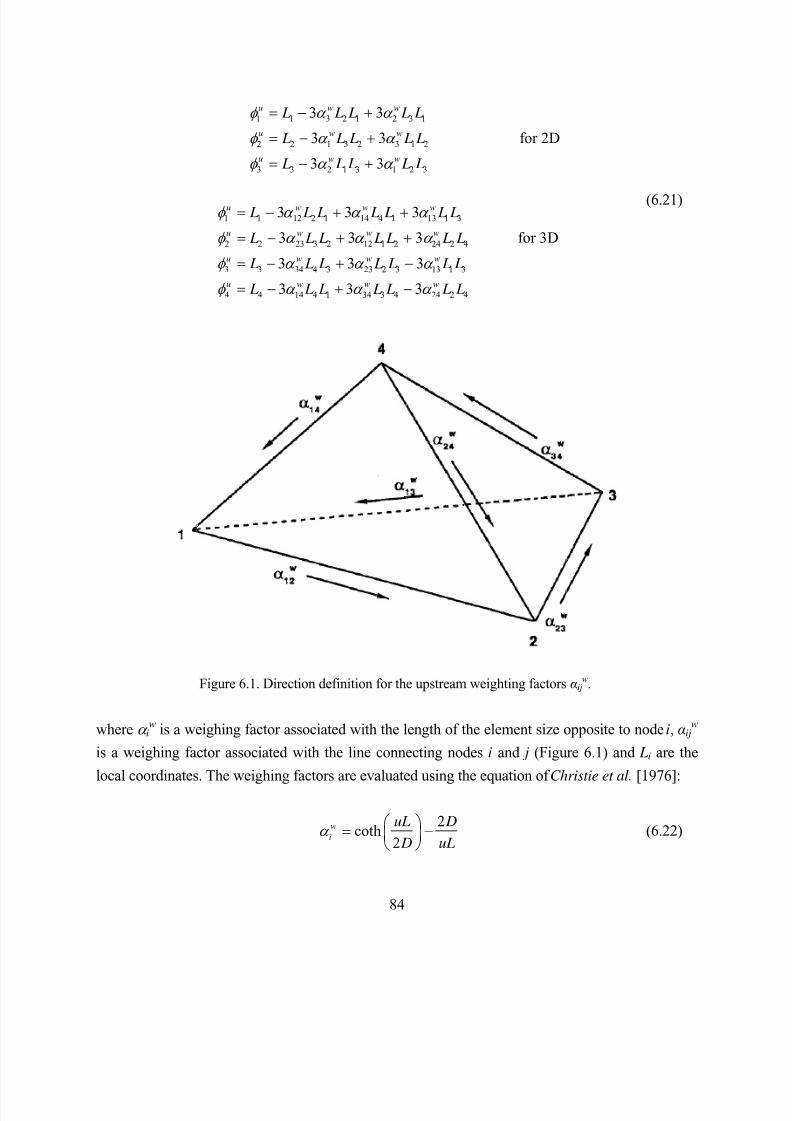
8/20/2019 HYDRUS3D Technical Manual.pdf
http://slidepdf.com/reader/full/hydrus3d-technical-manualpdf 114/260
84
1 1 3 2 1 2 3 1
2 2 1 3 2 3 1 2
3 3 2 1 3 1 2 3
1 1 12 2 1 14 4 1 13 1 3
2 2 23 3 2 12 1 2 24 2 4
3 3 34 4 3 23 2 3 13 1 3
4 4
3 3
3 3 for 2D
3 3
3 3 3
3 3 3 for 3D
3 3 3
3
u w w
u w w
u w w
u w w w
u w w w
u w w w
u
L L L L L
L L L L L
L L L L L
L L L L L L L
L L L L L L L
L L L L L L L
L
φ α α
φ α α
φ α α
φ α α α
φ α α α
φ α α α
φ
= − +
= − +
= − +
= − + +
= − + +
= − + −
= − 14 4 1 34 3 4 24 2 43 3w w w L L L L L Lα α α + −
(6.21)
Figure 6.1. Direction definition for the upstream weighting factors αijw.
where α iw is a weighing factor associated with the length of the element size opposite to node i, αij
w
is a weighing factor associated with the line connecting nodes i and j (Figure 6.1) and Li are the
local coordinates. The weighing factors are evaluated using the equation of Christie et al. [1976]:
2coth
2w
i
uL D
D uLα
= −
(6.22)
8/20/2019 HYDRUS3D Technical Manual.pdf
http://slidepdf.com/reader/full/hydrus3d-technical-manualpdf 115/260
85
where u, D and L are the flow velocity, dispersion coefficient and length associated with side i. The
weighing functions φ u ensure that relatively more weight is placed on the flow velocities of nodes
located at the upstream side of an element. Evaluating the integrals in (6.3) shows that the
following additional terms must be added to the entries of the global matrix S nm in equation (6.6) intwo-dimensional formulation:
'1 1 1 2 3 2 2 3 3 2 3
1 2 3 2 2 3 3 2 3
- [2 ( - ) ( - 2 ) (2 - )] -40
- [2 ( - ) ( - 2 ) (2 - )]40
je e w w w w w w
j j x x x
j w w w w w w
z z z
bS S q q q
cq q q
α α α α α α
α α α α α α
= + +
+ +
(6.23)
'2 2 1 3 1 2 3 1 3 3 1
1 3 1 2 3 1 3 3 1
- [ (2 - ) 2 ( - ) ( - 2 )] -
40 - [ (2 - ) 2 ( - ) ( - 2 )]
40
je e w w w w w w
j j x x x
j w w w w w w
z z z
bS S q q q
cq q q
α α α α α α
α α α α α α
= + +
+ + (6.24)
'3 3 1 1 2 2 1 2 3 1 2
1 1 2 2 1 2 3 1 2
- [ ( - 2 ) (2 - ) 2 ( - )] -40
- [ ( - 2 ) (2 - ) 2 ( - )]40
je e w w w w w w
j j x x x
j w w w w w w
z z z
bS S q q q
cq q q
α α α α α α
α α α α α α
= + +
+ +
(6.25)
and in three-dimensional formulation
( ) ( )
( ) ( )
( ) ( )
1 1 1 12 14 13 2 12 14 13
3 12 14 13 4 12 14 13
1 1
[ 2 2 2 2240
2 2 ]
............... ..... .............. ....240 240
je e w w w w w w
j j x x
w w w w w w
x x
j j
y z
bS S q q
q q
c d q q
α α α α α α
α α α α α α
′ = − − + + + − + + +
+ − + + + − + + −
− − + − − +
(6.26)
( ) ( )
( ) ( )
( ) ( )
2 2 1 23 112 24 2 23 12 24
3 23 12 24 4 23 12 24
1 1
[ 2 2 2 2240
2 2 ]
............... ..... .............. ....240 240
je e w w w w w w
j j x x
w w w w w w
x x
j j y z
bS S q q
q q
c d q q
α α α α α α
α α α α α α
′ = − − + + + − + + +
+ − + + + − + + −
− − + − − +
(6.27)
8/20/2019 HYDRUS3D Technical Manual.pdf
http://slidepdf.com/reader/full/hydrus3d-technical-manualpdf 116/260
86
( ) ( )
( ) ( )
( ) ( )
3 3 1 34 23 13 2 34 23 13
3 34 23 13 4 34 23 13
1 1
[ 2 2240
2 2 2 2 ]
............... ..... .............. ....240 240
je e w w w w w w j j x x
w w w w w w x x
j j y z
bS S q q
q q
c d
q q
α α α α α α
α α α α α α
′ = − − + − + − + − +
+ − + − + − + − −
− − + − − +
(6.28)
( ) ( )
( ) ( )
( ) ( )
4 4 1 14 34 24 2 14 34 24
3 14 34 24 4 14 34 24
1 1
[ 2 2240
2 2 2 2 ]
............... ..... .............. ....240 240
je e w w w w w w j j x x
w w w w w w x x
j j y z
bS S q q
q q
c d q q
α α α α α α
α α α α α α
′ = − − + − + − + − +
+ − + − + − + − −
− − + − − +
(6.29)
The weighing factors are applied only to those element sides that are inclined within 10
degrees from the flow direction.
6.4.3. Implementation of First-Type Boundary Conditions
Individual equations in the global matrix equation which correspond to nodes at which the
concentration is prescribed are replaced by new equations:
0nm m n
c cδ = (6.30)
where cn0 is the prescribed value of the concentration at node n. This is done only when Gaussian
elimination is used to solve the matrix equation. A similar procedure as for water flow (described in
Section 5.3.4) is applied when the ORTHOMIN method is used. Because of asymmetry of the
global matrix [G], no additional manipulations are needed in the resulting system of equations as
was the case for the water flow solution.
The total material flux, QnT , through a boundary at node n consists of the dispersive flux,
Qn D, and the convective flux, Qn
A:
T D A
n n nQ Q Q= + (6.31)
8/20/2019 HYDRUS3D Technical Manual.pdf
http://slidepdf.com/reader/full/hydrus3d-technical-manualpdf 117/260
87
The dispersive boundary nodal flux is not known explicitly but must be calculated from equation
(6.4). Hence, the dispersion flux, Qn D, for node n can be calculated as
( ) ( )1
1 11 1 j j
D j j j j j j n nn nm nm m n n nn
c cQ S S c f f Q
t ε ε ε ε ε
++ + + − = − + − − − − − ∆
(6.32)
The convective flux is evaluated as
A
n n nQ Q c= (6.33)
where the fluid flux Qn is known from the solution of the water flow equation.
6.4.4. Implementation of Third-Type Boundary Conditions
Equation (3.43) is rewritten as follows
( )0ij i i i
j
c D n q n c c
xθ
′∂= −
∂ (6.34)
When substituted into the last term of (6.3), the boundary integral becomes
0e N
ij i n n n n n
e j
c D n d Q c Q c
xθ φ
Γ
′∂Γ = −
∂∑ ∫ (6.35)
The first term on the right-hand side of (6.35) represents the convective flux. This term is
incorporated into the coefficient matrix [S ] of (6.4). The last term of (6.35) represents the total
material flux, which is added to the known vector f .
At nodes where free outflow of water and its dissolved solutes takes place, the exit
concentration c0 is equal to the local (nodal) concentration cn. In this case the dispersive flux
8/20/2019 HYDRUS3D Technical Manual.pdf
http://slidepdf.com/reader/full/hydrus3d-technical-manualpdf 118/260
88
becomes zero and the total material flux through the boundary is evaluated as
T
n n nQ Q c= (6.36)
The Cauchy boundary condition for volatile solutes is treated in a similar way. Equation(3.45) is rewritten as follows
( )0 - ( - )g
ij i i i g atm
j
Dc D n q n c c k c g
x d θ
′∂= −
∂ (6.37)
Again, when substituted into the last term of (6.3), the boundary integral becomes
0 - ( - )e N
gij i n n n n n g n atm
e j
D Lc D n d Q c Q c k c g x d
θ φ Γ
∆′∂ Γ = −∂∑ ∫ (6.38)
where ∆ L is the length of the boundary associated with node n. The last term of (6.38) representing
the gas diffusion flux through the stagnant boundary layer at the soil surface is directly added to the
vector f in equation (6.9), whereas the term containing k g and unknown concentration cn is
incorporated into the coefficient matrix [S ]. The other terms on the right-hand side of (6.38) are
treated in the same way as described above for equation (6.35).
6.4.5. Mass Balance Calculations
The total amount of mass in the entire flow domain, or in a preselected subregion, is given
by
1
( )
1e e
k s
v v g
e e
k c M c a g s d a k f c s d
c
β
β θ ρ θ ρ ρ
η
−
Ω Ω
= + + Ω = + + + Ω
+
∑ ∑∫ ∫ (6.39)
8/20/2019 HYDRUS3D Technical Manual.pdf
http://slidepdf.com/reader/full/hydrus3d-technical-manualpdf 119/260
89
The summation is taken over all elements within the specified region. The equations in this section
pertain only to the equilibrium or chemical nonequilibrium models; the mass balance equations for
physical nonequilibrium transport are very similar as those for chemical nonequilibirum.
The cumulative amounts M 0 and M 1 of solute removed from the flow region by zero- and
first-order reactions, respectively, are calculated as follows
1
1
01 ,1 ,1 ,1
0
1, 1 1' ' '
1 , 1 , 1 , 1 , 1 11 10
', 1 1 , , ,
- ( )
- [1
]
e
k
k
e
t
w s g ve
t s k k k
w k s k g k v g k k e k k
k s k k w k s k g k v
M a d dt
k c M f a k c
c
s a d dt
β
β
γ θ γ ρ γ
µ θ µ ρ µ η
µ ρ γ θ γ ρ γ
−
−
Ω
−− −
− − − − −− −Ω
− −
= + + Ω
= + + + +
+ + + + Ω
∑∫ ∫
∑∫ ∫ (6.40)
1
' ' '1
0
'
( ) ( ) ( )1
( )
e
t
sw w s s g g v g
e
k
s s
k c f a k c M
c
s d dt
β
β µ µ θ µ µ ρ µ µ η
µ µ ρ
−
Ω
= + + + + + + +
+ + Ω
∑∫ ∫ (6.41)
whereas the cumulative amount M r of solute taken up by plant roots is given by
0 R e
t
r s
e
M Sc d dt Ω
= Ω∑∫ ∫ (6.42)
where e R represents the elements making up the root zone.
Finally, when all boundary material fluxes, decay reactions, and root uptake mass fluxes
have been computed, the following mass balance should hold for the flow domain as a whole:
0 10
0
t
T
t n r
n
M M Q dt M M M Γ
− = + + −∑∫ (6.43)
where M t and M 0 are the amounts of solute in the flow region at times t and zero, respectively, as
calculated with (6.39), and nΓ represents nodes located along the boundary of the flow domain or at
internal sinks and/or sources. The difference between the left- and right-hand sides of (6.43)
8/20/2019 HYDRUS3D Technical Manual.pdf
http://slidepdf.com/reader/full/hydrus3d-technical-manualpdf 120/260
90
represents the absolute error, εac, in the solute mass balance. Similarly as for water flow, the
accuracy of the numerical solution for solute transport is evaluated by using the relative error, εr c
[%], in the solute mass balance as follows
0 10
0
100
max ,
c
ac
r t
e e T
t r n
e n
M M M M M Q dt
ε ε
Γ
=
− + + + ∑ ∑∫
(6.44)
where M 0e and M t
e are the amounts of solute in element e at times 0 and t , respectively. Note again
that HYDRUS does not relate the absolute error to the total amount of mass in the flow region.
Instead, the program uses as a reference the maximum value of (1) the absolute change in element
concentrations as summed over all elements, and (2) the sum of the absolute values of all
cumulative solute fluxes across the flow boundaries including those resulting from sources and
sinks in the flow domain.
The total amount of heat energy in the entire flow domain, or in a preselected subregion, is
given by
( )e
A
n n o o w g v
e
W c c C C a T d θ θ θ
Ω
= + + + Ω∑∫ (6.45)
where T A is the absolute temperature [K]. The summation is taken over all elements within the
specified region.
8/20/2019 HYDRUS3D Technical Manual.pdf
http://slidepdf.com/reader/full/hydrus3d-technical-manualpdf 121/260
91
6.4.6. Oscillatory Behavior
Numerical solutions of the transport equation often exhibit oscillatory behavior and/or
excessive numerical dispersion near relatively sharp concentration fronts. These problems can be
especially serious for convection-dominated transport characterized by small dispersivities. Oneway to partially circumvent numerical oscillations is to use upstream weighing as discussed in
Section 6.4.2. Undesired oscillations can often be prevented also by selecting an appropriate
combination of space and time discretizations. Two dimensionless numbers may be used to
characterize the space and time discretizations. One of these is the grid Peclet number, Peie, which
defines the predominant type of the solute transport (notably the ratio of the convective and
dispersive transport terms) in relation to coarseness of the finite element grid:
ei ii
ii
q xPe Dθ
∆= (6.46)
where Δ xi is the characteristic length of a finite element. The Peclet number increases when the
convective part of the transport equation dominates the dispersive part, i.e., when a relatively steep
concentration front is present. To achieve acceptable numerical results, the spatial discretization
must be kept relatively fine to maintain a low Peclet number. Numerical oscillation can be virtually
eliminated when the local Peclet numbers do not exceed about 5. However, acceptably small
oscillations may be obtained with local Peclet numbers as high as 10 [ Huyakorn and Pinder , 1983].
Undesired oscillation for higher Peclet numbers can be effectively eliminated by using upstream
weighing (see Section 6.4.2).
A second dimensionless number which characterizes the relative extent of numerical
oscillations is the Courant number, Cr ie. The Courant number is associated with the time
discretization as follows
e ii
i
q t Cr
R xθ
∆=
∆ (6.47)
Three stabilizing options are used in HYDRUS to avoid oscillations in the numerical
solution of the solute transport equation [Šimůnek and van Genuchten, 1994]. One option is
8/20/2019 HYDRUS3D Technical Manual.pdf
http://slidepdf.com/reader/full/hydrus3d-technical-manualpdf 122/260
92
upstream weighing (see Section 6.4.2), which effectively eliminates undesired oscillations at
relatively high Peclet numbers. A second option for minimizing or eliminating numerical
oscillations uses the criterion developed by Perrochet and Berod [1993]
2sPe Cr ω ⋅ ≤ = (6.48)
where ωs is the performance index [-]. This criterion indicates that convection-dominated transport
problems having large Pe numbers can be safely simulated provided Cr is reduced according to
(6.48) [Perrochet and Berod , 1993]. When small oscillations in the solution can be tolerated, ω s can
be increased to about 5 or 10.
A third stabilization option implemented in HYDRUS also utilizes criterion (6.48).
However, instead of decreasing Cr to satisfy equation (6.48), this option introduces artificial
dispersion to decrease the Peclet number. The amount of additional longitudinal dispersion, L D [L], is given by [Perrochet and Berod , 1993]
d L L
s
q t D D D
R q
θ τ
θ ω
∆= − − (6.49)
The maximum permitted time step is calculated for all three options, as well as with the additional
requirement that the Courant number must remain less than or equal to 1. The time step calculated
in this way is subsequently used as one of the time discretization rules (rule No. B) discussed insection 5.3.3.
8/20/2019 HYDRUS3D Technical Manual.pdf
http://slidepdf.com/reader/full/hydrus3d-technical-manualpdf 123/260
93
7. PARAMETER OPTIMIZATION
Parameter optimization is an indirect approach for estimating the unsaturated soil hydraulic
and/or solute transport parameters from transient flow and/or transport data. Inverse methods are
typically based upon the minimization of a suitable objective function, which expresses thediscrepancy between the observed values and the predicted system response. Soil hydraulic
properties for this purpose are assumed to be described by an analytical model with unknown
parameter values (see Section 2.3). The system response is represented by a numerical solution of
the flow equation, augmented with the parameterized hydraulic functions, selected transport
parameters, and suitable initial and boundary conditions. Initial estimates of the optimized system
parameters are then iteratively improved during the minimization process until a desired degree of
precision is obtained. This methodology was originally applied to one-step and multi-step column
outflow data generated in the laboratory [see for example Kool et al., 1985; van Dam et al., 1994],
and laboratory or field transport data during steady-state water flow [van Genuchten, 1981; Toride
et al., 1995]. HYDRUS implements parameter optimization also for estimating the solute transport
and reaction parameters from transient water flow and/or solute transport experiments.
7.1. Definition of the Objective Function
The objective function Φ to be minimized during the parameter estimation process may be
defined as [Šimůnek et al., 1998]:
2*,
1 1
2*
1 1
2*
1
( , , ) [ ( , ) - ( , , )]
[ ( ) - ( , )]
[ - ]ˆ
q q j
p p j
b
m n
j i j j i j i j i
m n
j ij j i j i j i
n
j j j j
v w g t g t
v w p p
b bv
θ θ
= =
= =
=
Φ = +
+ +
+
∑ ∑
∑ ∑
∑
b q p x x b
b (7.1)
where the first term on the right-hand side represents deviations between the measured and
calculated space-time variables (e.g., observed pressure heads, water contents, and/or
concentrations at different locations and/or time in the flow domain, or the actual or cumulative
8/20/2019 HYDRUS3D Technical Manual.pdf
http://slidepdf.com/reader/full/hydrus3d-technical-manualpdf 124/260
94
flux versus time across a boundary of specified type). In this term, mq is the number of different sets
of measurements, nqj is the number of measurements in a particular measurement set, q j*( x ,t i)
represents specific measurements at time t i for the jth measurement set at location x(r,z), q j( x ,t i , b)
are the corresponding model predictions for the vector of optimized parameters b (e.g., θ r , θ s , α , n,
K s, Dl, k g,k , ...), and v j and wi,j are weights associated with a particular measurement set or point,respectively. The second term of (7.1) represents differences between independently measured and
predicted soil hydraulic properties (e.g., retention, θ (h) and/or hydraulic conductivity, K (θ ) or K (h)
data), while the terms m p, n pj, p j*(θ i), p j(θ i , b), jv j and ,i jw have similar meanings as for the first
term but now for the soil hydraulic properties. The last term of (7.1) represents a penalty function
for deviations between prior knowledge of the soil hydraulic parameters, b j*, and their final
estimates, b j, with nb being the number of parameters with prior knowledge and ˆ jv representing
pre-assigned weights. Estimates, which make use of prior information (such as those used in the
third term of (7.1)) are known as Bayesian estimates. We note that the covariance (weighting)matrices, which provide information about the measurement accuracy, as well as any possible
correlation between measurement errors and/or parameters, are assumed to be diagonal in this
study. The weighting coefficients v j , which minimize differences in weighting between different
data types because of different absolute values and numbers of data involved, are given by
[Clausnitzer and Hopmans, 1995]:
2
1 j
j j
=n
ν σ
(7.2)
which causes the objective function to become the average weighted squared deviation normalized
by the measurement variances σ j2.
7.2. Marquardt-Levenberg Optimization Algorithm
Minimization of the objective function Φ is accomplished by using the Levenberg-
Marquardt nonlinear minimization method (a weighted least-squares approach based on
Marquardt's maximum neighborhood method) [ Marquardt , 1963]. This method combines the
Newton and steepest descend methods, and generates confidence intervals for the optimized
8/20/2019 HYDRUS3D Technical Manual.pdf
http://slidepdf.com/reader/full/hydrus3d-technical-manualpdf 125/260
95
parameters. The method was found to be very effective and has become a standard in nonlinear
least-squares fitting among soil scientists and hydrologists [van Genuchten, 1981; Kool et al., 1985,
1987].
7.3. Statistics of the Inverse Solution
As part of the inverse solution, HYDRUS produces a correlation matrix which specifies
degree of correlation between the fitted coefficients. The correlation matrix quantifies changes in
model predictions caused by small changes in the final estimate of a particular parameter, relative to
similar changes as a result of changes in the other parameters. The correlation matrix reflects the
nonorthogonality between two parameter values. A value of ±1 suggests a perfect linear correlation
whereas 0 indicates no correlation at all. The correlation matrix may be used to select which
parameters, if any, are best kept constant in the parameter estimation process because of high
correlation.
An important measure of the goodness of fit is the r 2 value for regression of the observed, y
i, versus fitted, yi( b), values:
2
2
2 22 2
ˆˆ
ˆ( ) ( )ˆ
ii
i ii
i
i i
i i i
i i
y yw y - y
wr =
y yw - - y yw w
∑ ∑∑
∑
∑ ∑
∑ ∑ ∑ ∑
(7.3)
The r 2 value is a measure of the relative magnitude of the total sum of squares associated with the
fitted equation; a value of 1 indicates a perfect correlation between the fitted and observed values.
HYDRUS provides additional statistical information about the fitted parameters such as the
mean, standard error, T-value, and the lower and upper confidence limits (given in output file
FIT.OUT). The standard error, s(b j), is estimated from knowledge of the objective function, the
number of observations, the number of unknown parameters to be fitted, and an inverse matrix[ Daniel and Wood , 1971]. The T -value is obtained from the mean and standard error using the
equation
8/20/2019 HYDRUS3D Technical Manual.pdf
http://slidepdf.com/reader/full/hydrus3d-technical-manualpdf 126/260
96
( )
j
j
bT
s b= (7.4)
The values for T and s(b j) provide absolute and relative measures of the deviations around themean. HYDRUS also specifies the upper and lower bounds of the 95% confidence level around
each fitted parameter b j. It is desirable that the real value of the target parameter always be located
in a narrow interval around the estimated mean as obtained with the optimization program. Large
confidence limits indicate that the results are not very sensitive to the value of a particular
parameter.
Finally, because of possible problems related to convergence and parameter uniqueness, we
recommend to routinely rerun the program with different initial parameter estimates to verify that
the program indeed converges to the same global minimum in the objective function. This is
especially important for field data sets, which often exhibit considerable scatter in themeasurements, or may cover only a narrow range of soil water contents, pressure heads, and/or
concentrations. Whereas HYDRUS will not accept initial estimates that are out of range, it is
ultimately the user's responsibility to select meaningful initial estimates. Parameter optimization is
implemented only for two-dimensional problems.
8/20/2019 HYDRUS3D Technical Manual.pdf
http://slidepdf.com/reader/full/hydrus3d-technical-manualpdf 127/260
97
8. PROBLEM DEFINITION
8.1. Construction of Finite Element Mesh
The finite element mesh is constructed by dividing the flow region for two-dimensional problems into quadrilateral and/or triangular elements or for three-dimensional problems into
tetrahedral, hexahedral and/or triangular prismatic elements (Fig. 8.1) whose shapes are defined by
the coordinates of the nodes that form the element corners. The program automatically subdivides
the quadrilaterals into triangles (or hexahedrals and triangular prisms into tetrahedrals), which are
then treated as subelements. Two different ways are possible to subdivide the hexahedrals into
tetrahedrals, whereas six different possibilities exist for subdividing the triangular prisms into
tetrahedrals (see Fig. 8.1).
If two neighboring hexahedral elements are subdivided in the same way (e.g., options 2a or
2b in Fig. 8.1), the newly formed edges on a common surface will cross each other, a feature whichis not allowed. Two neighboring hexahedral elements should therefore always use both options 2a
and 2b as shown in Figure 8.1, so that the newly formed edges on the common surface will
coincide. Therefore, it is necessary to give not only the corner nodes, which define an element, but
also the code, which specifies how a particular element is to be subdivided into subelements (this is
done automatically if the graphical user interface is used). It is necessary to always realize how the
neighboring elements are going to be subdivided, and to input also the proper code specifying the
subdivision. Having high flexibility in terms of possible subdivisions into subelements is important,
especially for unstructured finite element meshes using triangular prisms.Transverse lines [ Neuman, 1974] formed by element boundaries must transect the mesh
along the general direction of its shortest dimension. These transverse lines should be continuous
and non-intersecting, but need not be straight. The nodes are numbered sequentially from 1 to
NumNP (total number of nodes) by proceeding along each transverse line in the same direction.
Elements are numbered in a similar manner. The maximum number of nodes on any transverse line,
IJ , is used to determine the effective size of the finite element matrix (i.e., its band width). To
minimize memory and time requirements, IJ should be kept as small as possible. The above rules
for defining the finite element mesh apply only when Gaussian elimination is used to solve the
matrix equations. Iterative methods (such as the conjugate gradient and ORTHOMIN methods) arenot so restrictive since only non-zero entries in the coefficient matrix are stored in memory, and
since the computational efficiency is less dependent upon the bandwidth of the matrix as compared
8/20/2019 HYDRUS3D Technical Manual.pdf
http://slidepdf.com/reader/full/hydrus3d-technical-manualpdf 128/260
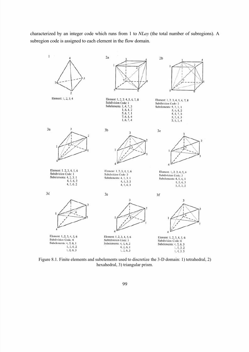
8/20/2019 HYDRUS3D Technical Manual.pdf
http://slidepdf.com/reader/full/hydrus3d-technical-manualpdf 129/260
99
characterized by an integer code which runs from 1 to NLay (the total number of subregions). A
subregion code is assigned to each element in the flow domain.
Figure 8.1. Finite elements and subelements used to discretize the 3-D domain: 1) tetrahedral, 2)hexahedral, 3) triangular prism.
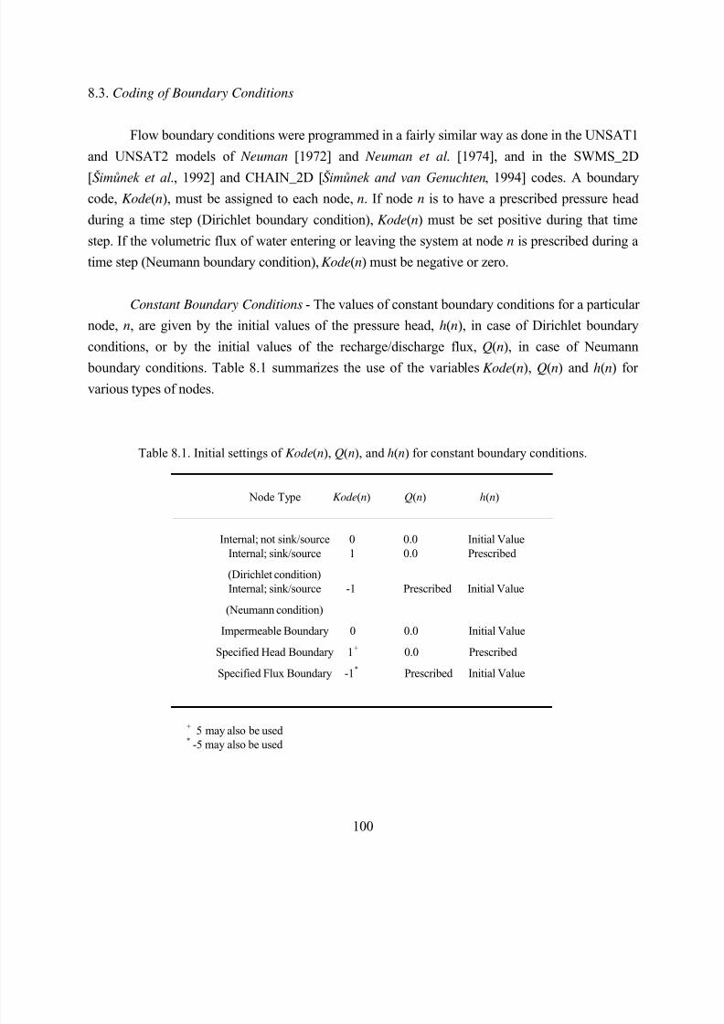
8/20/2019 HYDRUS3D Technical Manual.pdf
http://slidepdf.com/reader/full/hydrus3d-technical-manualpdf 130/260
100
8.3. Coding of Boundary Conditions
Flow boundary conditions were programmed in a fairly similar way as done in the UNSAT1
and UNSAT2 models of Neuman [1972] and Neuman et al. [1974], and in the SWMS_2D
[Šimůnek et al ., 1992] and CHAIN_2D [Šimůnek and van Genuchten, 1994] codes. A boundarycode, Kode(n), must be assigned to each node, n. If node n is to have a prescribed pressure head
during a time step (Dirichlet boundary condition), Kode(n) must be set positive during that time
step. If the volumetric flux of water entering or leaving the system at node n is prescribed during a
time step (Neumann boundary condition), Kode(n) must be negative or zero.
Constant Boundary Conditions - The values of constant boundary conditions for a particular
node, n, are given by the initial values of the pressure head, h(n), in case of Dirichlet boundary
conditions, or by the initial values of the recharge/discharge flux, Q(n), in case of Neumann
boundary conditions. Table 8.1 summarizes the use of the variables Kode(n), Q(n) and h(n) for
various types of nodes.
Table 8.1. Initial settings of Kode(n), Q(n), and h(n) for constant boundary conditions.
Node Type Kode(n) Q(n) h(n)
Internal; not sink/source 0 0.0 Initial ValueInternal; sink/source 1 0.0 Prescribed
(Dirichlet condition)Internal; sink/source -1 Prescribed Initial Value
(Neumann condition)
Impermeable Boundary 0 0.0 Initial Value
Specified Head Boundary 1+ 0.0 Prescribed
Specified Flux Boundary -1* Prescribed Initial Value
+ 5 may also be used* -5 may also be used
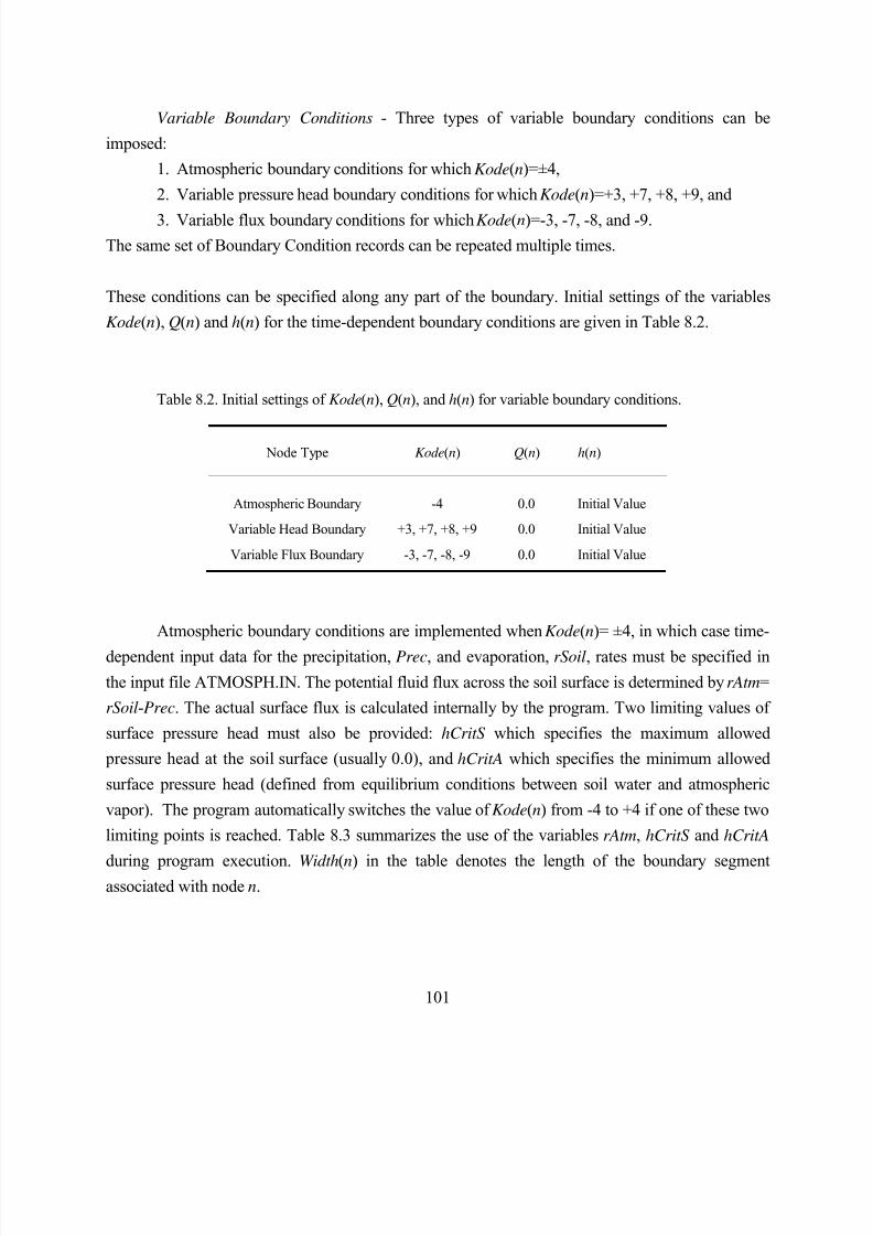
8/20/2019 HYDRUS3D Technical Manual.pdf
http://slidepdf.com/reader/full/hydrus3d-technical-manualpdf 131/260
101
Variable Boundary Conditions - Three types of variable boundary conditions can be
imposed:
1. Atmospheric boundary conditions for which Kode(n)=±4,
2. Variable pressure head boundary conditions for which Kode(n)=+3, +7, +8, +9, and
3. Variable flux boundary conditions for which Kode(n)=-3, -7, -8, and -9.The same set of Boundary Condition records can be repeated multiple times.
These conditions can be specified along any part of the boundary. Initial settings of the variables
Kode(n), Q(n) and h(n) for the time-dependent boundary conditions are given in Table 8.2.
Table 8.2. Initial settings of Kode(n), Q(n), and h(n) for variable boundary conditions.
Node Type Kode(n) Q(n) h(n)
Atmospheric Boundary -4 0.0 Initial Value
Variable Head Boundary +3, +7, +8, +9 0.0 Initial Value
Variable Flux Boundary -3, -7, -8, -9 0.0 Initial Value
Atmospheric boundary conditions are implemented when Kode(n)= ±4, in which case time-
dependent input data for the precipitation, Prec, and evaporation, rSoil, rates must be specified inthe input file ATMOSPH.IN. The potential fluid flux across the soil surface is determined by rAtm=
rSoil-Prec. The actual surface flux is calculated internally by the program. Two limiting values of
surface pressure head must also be provided: hCritS which specifies the maximum allowed
pressure head at the soil surface (usually 0.0), and hCritA which specifies the minimum allowed
surface pressure head (defined from equilibrium conditions between soil water and atmospheric
vapor). The program automatically switches the value of Kode(n) from -4 to +4 if one of these two
limiting points is reached. Table 8.3 summarizes the use of the variables rAtm, hCritS and hCritA
during program execution. Width(n) in the table denotes the length of the boundary segmentassociated with node n.
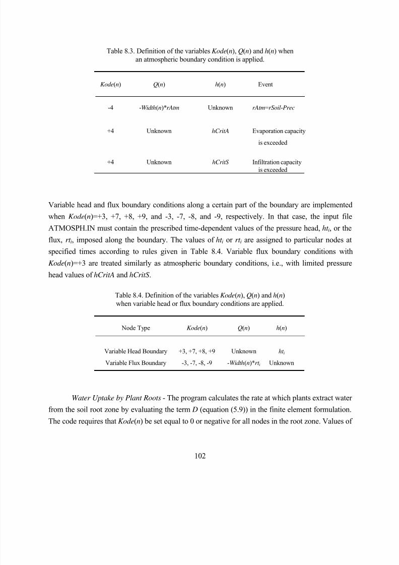
8/20/2019 HYDRUS3D Technical Manual.pdf
http://slidepdf.com/reader/full/hydrus3d-technical-manualpdf 132/260
102
Table 8.3. Definition of the variables Kode(n), Q(n) and h(n) whenan atmospheric boundary condition is applied.
Kode(n) Q(n) h(n) Event
-4 -Width(n)*rAtm Unknown rAtm=rSoil-Prec
+4 Unknown hCritA Evaporation capacity
is exceeded
+4 Unknown hCritS Infiltration capacityis exceeded
Variable head and flux boundary conditions along a certain part of the boundary are implemented
when Kode(n)=+3, +7, +8, +9, and -3, -7, -8, and -9, respectively. In that case, the input file
ATMOSPH.IN must contain the prescribed time-dependent values of the pressure head, ht i, or the
flux, rt i, imposed along the boundary. The values of ht i or rt i are assigned to particular nodes at
specified times according to rules given in Table 8.4. Variable flux boundary conditions with
Kode(n)=+3 are treated similarly as atmospheric boundary conditions, i.e., with limited pressure
head values of hCritA and hCritS .
Table 8.4. Definition of the variables Kode(n), Q(n) and h(n)when variable head or flux boundary conditions are applied.
Node Type Kode(n) Q(n) h(n)
Variable Head Boundary +3, +7, +8, +9 Unknown ht i
Variable Flux Boundary -3, -7, -8, -9 -Width(n)*rt i Unknown
Water Uptake by Plant Roots - The program calculates the rate at which plants extract waterfrom the soil root zone by evaluating the term D (equation (5.9)) in the finite element formulation.
The code requires that Kode(n) be set equal to 0 or negative for all nodes in the root zone. Values of
8/20/2019 HYDRUS3D Technical Manual.pdf
http://slidepdf.com/reader/full/hydrus3d-technical-manualpdf 133/260
103
the potential transpiration rate, rRoot , must be specified at preselected times in the input file
ATMOSPH.IN. Actual transpiration rates are calculated internally by the program as discussed in
Section 2.2. The root uptake parameters are taken from an input file SELECTOR.IN. Values of the
function Beta(n), which describes the potential water uptake distribution over the root zone
(equation (2.9)), must be specified for each node in the flow domain (see the description of inputBlock I in Table 10.8 of Section 10). All parts of the flow region where Beta(n)>0 are treated as the
soil root zone.
Deep Drainage from the Soil Profile - Vertical drainage, q(h), across the lower boundary of
the soil profile is sometimes approximated by a flux which depends on the position of groundwater
level (e.g., Hopmans and Stricker , 1989). If available, such a relationship can be implemented in
the form of a variable flux boundary condition for which Kode(n)=-6. This boundary condition is
implemented in HYDRUS by setting the logical variableqGWLF
in the input file BOUNDARY.INequal to ".true.". The discharge rate Q(n) assigned to node n is determined by the program as
Q(n)=-Width(n)*q(h) where h is the local value of the pressure head, and q(h) is given by
( ) ( )exp 0qh qhq h A B h GWL L= − − (8.1)
where Aqh and Bqh are empirical parameters which must be specified in the input file
BOUNDARY.IN, together with GWL0L which represents the reference position of the groundwater
level (usually set equal to the z-coordinate of the soil surface).
Free Drainage - Unit vertical hydraulic gradient boundary conditions can be implemented
in the form of a variable flux boundary condition for which Kode(n)=-6. This boundary condition is
implemented in HYDRUS by setting the logical variable FreeD in the input file BOUNDARY.IN
equal to ".true.". The program determines the discharge rate Q(n) assigned to node n as
Q(n)=-Width(n)*K (h), where h is the local value of the pressure head, and K (h) is the hydraulic
conductivity corresponding to this pressure head. In Version 2.0 users can specify other than unit
gradient boundary conditions.
Seepage Faces - The initial settings of the variables Kode(n), Q(n) and h(n) for nodes along
a seepage face are summarized in Table 8.5. All potential seepage faces must be identified before
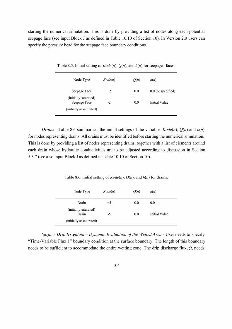
8/20/2019 HYDRUS3D Technical Manual.pdf
http://slidepdf.com/reader/full/hydrus3d-technical-manualpdf 134/260
104
starting the numerical simulation. This is done by providing a list of nodes along each potential
seepage face (see input Block J as defined in Table 10.10 of Section 10). In Version 2.0 users can
specify the pressure head for the seepage face boundary conditions.
Table 8.5. Initial setting of Kode(n), Q(n), and h(n) for seepage faces.
Node Type Kode(n) Q(n) h(n)
Seepage Face +2 0.0 0.0 (or specified)
(initially saturated)Seepage Face -2 0.0 Initial Value
(initially unsaturated)
Drains - Table 8.6 summarizes the initial settings of the variables Kode(n), Q(n) and h(n)
for nodes representing drains. All drains must be identified before starting the numerical simulation.
This is done by providing a list of nodes representing drains, together with a list of elements around
each drain whose hydraulic conductivities are to be adjusted according to discussion in Section
5.3.7 (see also input Block J as defined in Table 10.10 of Section 10).
Table 8.6. Initial setting of Kode(n), Q(n), and h(n) for drains.
Node Type Kode(n) Q(n) h(n)
Drain +5 0.0 0.0
(initially saturated)Drain -5 0.0 Initial Value
(initially unsaturated)
Surface Drip Irrigation – Dynamic Evaluation of the Wetted Area - User needs to specify
“Time-Variable Flux 1” boundary condition at the surface boundary. The length of this boundary
needs to be sufficient to accommodate the entire wetting zone. The drip discharge flux, Q, needs
8/20/2019 HYDRUS3D Technical Manual.pdf
http://slidepdf.com/reader/full/hydrus3d-technical-manualpdf 135/260
105
to be entered in the “Var.Fl-1” column of the “Time Variable Boundary Conditions” dialog
window. Using Boundary Line Chart, one can see how the wetting zone expands in time.
Subsurface Drip Characteristic Function - User needs to specify “Time-Variable Flux 1”
boundary condition along the dripper boundary and hin in the “Var.H-1” column of the “Time
Variable Boundary Conditions” dialog window. A positive pressure indicates an irrigation periodand a negative pressure indicates a non-irrigation period.
Solute and Heat Transport Boundary Conditions - The original version 1.1. of SWMS_2D
[Šimůnek et al ., 1992] assumed a strict relationship between the boundary conditions for water flow
and solute transport. A first-type boundary condition for water flow forced the boundary condition
for solute transport also to be of the first-type. Similarly, a second-type boundary condition for
water flow induced a second- or third-type boundary condition for solute transport depending upon
direction of the water flux. These strict relationships between the boundary conditions for waterflow and solute transport have been abandoned in later versions. Selection of the type of boundary
condition for the solute transport is now much more independent of the boundary condition
implemented for water flow. The type of boundary condition to be invoked for solute or heat
transport is specified by the input variable KodCB or KodTB, respectively. A positive sign of this
variable means that a first-type boundary condition will be used. When KodCB (KodTB) is
negative, HYDRUS selects a third-type boundary condition when the calculated water flux is
directed into the region, or a second-type boundary condition when the water flux is zero or directed
out of the region. One exception to these rules occurs for atmospheric boundary conditions when
Kode(n)=±4 and Q(n)<0. HYDRUS assumes that solutes can leave the flow region acrossatmospheric boundaries only by gas diffusion. The solute flux in this situation becomes zero, i.e.,
c0=0 in equation (6.34). Cauchy and Neumann boundary conditions are automatically applied to
internal sinks/sources depending upon the direction of water flow. The dependence or
independence of the solute and heat boundary conditions on time or the system is still defined
through the variable Kode(n) as discussed above.
Although HYDRUS can implement first-type boundary conditions, we recommend users to
invoke third-type conditions where possible. This is because third-type conditions, in general, are
physically more realistic and preserve solute mass in the simulated system (e.g., van Genuchten andParker [1984]; Leij et al. [1991]).
For the user's convenience, Table 8.7 summarizes possible values of the different boundary
codes and their association with specific water flow and solute transport boundary conditions.
8/20/2019 HYDRUS3D Technical Manual.pdf
http://slidepdf.com/reader/full/hydrus3d-technical-manualpdf 136/260
106
8.4. Program Memory Requirements
One single parameter statement is used at the beginning of the code to define the problem
dimensions. All major arrays in the program are adjusted automatically according to thesedimensions. This feature makes it possible to change the dimensions of the problem to be simulated
without having to recompile all program subroutines. Different problems can be investigated by
changing the dimensions in the parameter statement at the beginning of the main program, and
subsequently linking all previously compiled subroutines with the main program when creating an
executable file. Table 8.8 lists the array dimensions, which must be defined in the parameter
statement.
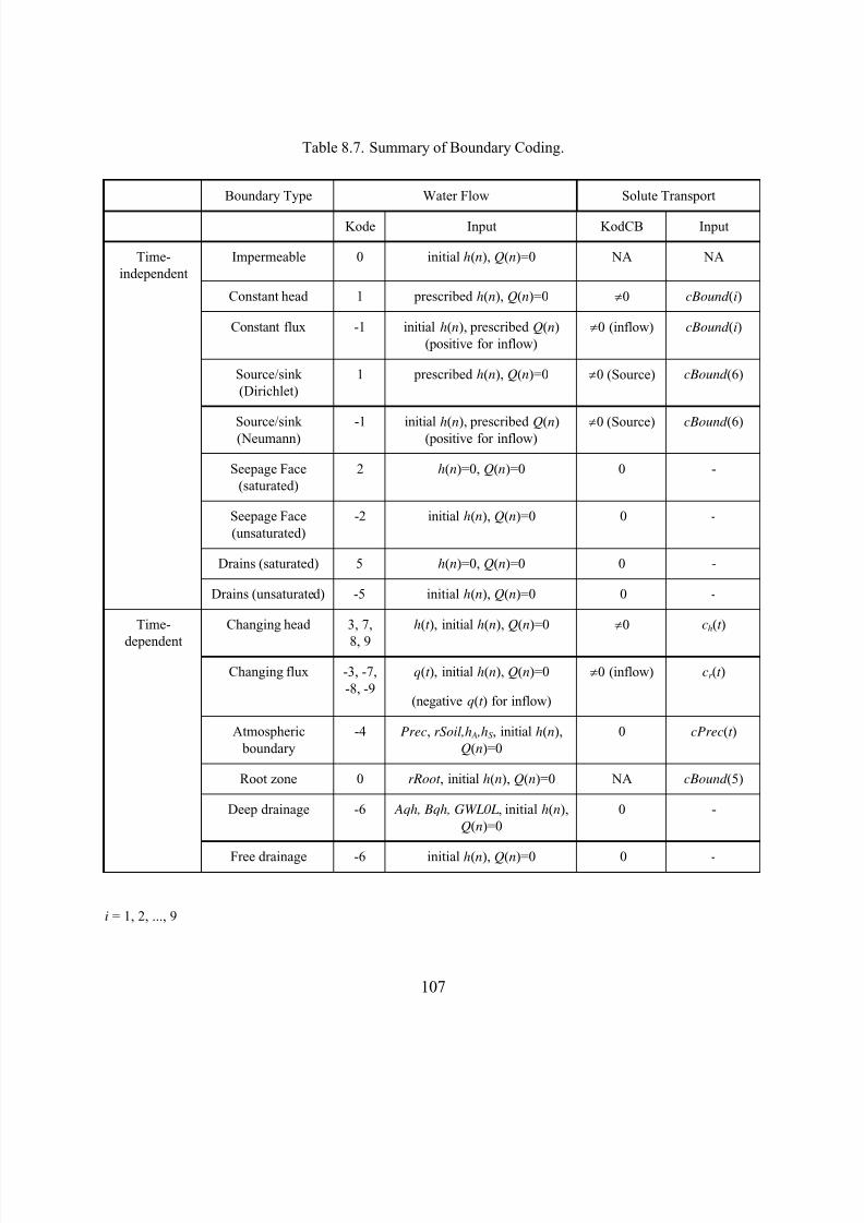
8/20/2019 HYDRUS3D Technical Manual.pdf
http://slidepdf.com/reader/full/hydrus3d-technical-manualpdf 137/260
107
Table 8.7. Summary of Boundary Coding.
Boundary Type Water Flow Solute Transport
Kode Input KodCB Input
Time-independent
Impermeable 0 initial h(n), Q(n)=0 NA NA
Constant head 1 prescribed h(n), Q(n)=0 ≠0 cBound (i)
Constant flux -1 initial h(n), prescribed Q(n)(positive for inflow)
≠0 (inflow) cBound (i)
Source/sink(Dirichlet)
1 prescribed h(n), Q(n)=0 ≠0 (Source) cBound (6)
Source/sink(Neumann) -1 initial h(n), prescribed Q(n)(positive for inflow) ≠0 (Source) cBound (6)
Seepage Face(saturated)
2 h(n)=0, Q(n)=0 0 -
Seepage Face(unsaturated)
-2 initial h(n), Q(n)=0 0 -
Drains (saturated) 5 h(n)=0, Q(n)=0 0 -
Drains (unsaturated) -5 initial h(n), Q(n)=0 0 -
Time-
dependent
Changing head 3, 7,
8, 9
h(t ), initial h(n), Q(n)=0 ≠0 ch(t )
Changing flux -3, -7,-8, -9
q(t ), initial h(n), Q(n)=0
(negative q(t ) for inflow)
≠0 (inflow) cr (t )
Atmospheric boundary
-4 Prec, rSoil,h A ,hS , initial h(n),Q(n)=0
0 cPrec(t )
Root zone 0 rRoot , initial h(n), Q(n)=0 NA cBound (5)
Deep drainage -6 Aqh, Bqh, GWL0L, initial h(n),Q(n)=0
0 -
Free drainage -6 initial h(n), Q(n)=0 0 -
i = 1, 2, ..., 9
8/20/2019 HYDRUS3D Technical Manual.pdf
http://slidepdf.com/reader/full/hydrus3d-technical-manualpdf 138/260
108
Table 8.8. List of array dimensions in HYDRUS.
Dimension Description
NumNPD Maximum number of nodes in finite element mesh
NumElD Maximum number of elements in finite element mesh
MBandD Maximum dimension of the bandwidth of matrix A whenGaussian elimination is used. Maximum number of nodesadjacent to a particular node, including itself, when iterativematrix solvers are used.
NumBPD Maximum number of boundary nodes for which Kode(n)≠0
NSeepD Maximum number of seepage faces
NumSPD Maximum number of nodes along a seepage face
NDrD Maximum number of drains
NElDrD Maximum number of elements surrounding a drain
NMatD Maximum number of materials
NTabD Maximum number of items in the table of hydraulic propertiesgenerated by the program for each soil material
NumKD Maximum number of available code number values (equals 6 in present version)
NSD Maximum number of solutes (equals 6 in present version)
NObsD Maximum number of observation nodes for which the pressure
head, the water content, temperature and concentration are printed at each time level
MNorth Maximum number of orthogonalizations performed wheniterative solvers are used
8.5. Matrix Equation Solvers
Discretization of the governing partial differential equations for water flow (2.1), solutetransport (3.11) and heat movement (4.1) leads to the system of linear equations
8/20/2019 HYDRUS3D Technical Manual.pdf
http://slidepdf.com/reader/full/hydrus3d-technical-manualpdf 139/260
109
[ ] A x b= (8.2)
in which matrix [ A] is symmetric for water flow and asymmetric for solute and heat transport.
The original version of SWMS_2D [Šimůnek et al., 1992] uses Gaussian elimination tosolve both systems of linear algebraic equations. The invoked solvers took advantage of the banded
nature of the coefficient matrices and, in the case of water flow, of the symmetric properties of the
matrix. Such direct solution methods have several disadvantages as compared to iterative methods.
Direct methods require a fixed number of operations (depending upon the size of the matrix), which
increases approximately by the square of the number of nodes [ Mendoza et al., 1991]. Iterative
methods, on the other hand, require a variable number of repeated steps, which increases at a much
smaller rate (about 1.5) with the size of a problem [ Mendoza et al., 1991]. A similar reduction also
holds for the memory requirement since iterative methods do not require one to store non-zero
matrix elements. Memory requirements, therefore, increase at a much smaller rate with the size ofthe problem when iterative solvers are used [ Mendoza et al., 1991]. Round-off errors also represent
less of a problem for iterative methods as compared to direct methods. This is because round-off
errors in iterative methods are self-correcting [ Letniowski, 1989]. Finally, for time-dependent
problems, a reasonable approximation of the solution (i.e., the solution at the previous time step)
exists for iterative methods, but not for direct methods [ Letniowski, 1989]. In general, direct
methods are more appropriate for relatively small problems, while iterative methods are more
suitable for larger problems.
Many iterative methods have been used in the past for handling large sparse matrixequations. These methods include Jacobi, Gauss-Seidel, alternating direction implicit (ADI), block
successive over-relaxation (BSSOR), successive line over-relaxation (SLOR), and strongly implicit
procedures (SIP), among others [ Letniowski, 1989]. More powerful preconditioned accelerated
iterative methods, such as the preconditioned conjugate gradient method (PCG) [ Behie and
Vinsome, 1982], were introduced more recently. Sudicky and Huyakorn [1991] gave three
advantages of the PCG procedure as compared to other iterative methods: PCG can be readily
modified for finite element methods with irregular grids, the method does not require iterative
parameters, and PCG usually outperforms its iterative counterparts for situations involving
relatively stiff matrix conditions.HYDRUS implements both direct and iterative methods for solving the system of linear
algebraic equations given by (8.2). Depending upon the size of matrix [ A], we use either direct
8/20/2019 HYDRUS3D Technical Manual.pdf
http://slidepdf.com/reader/full/hydrus3d-technical-manualpdf 140/260
110
Gaussian elimination or the preconditioned conjugate gradient method [ Mendoza et al., 1991] for
water flow and the ORTHOMIN (preconditioned conjugate gradient squared) procedure [ Mendoza
et al., 1991] for solute transport. Gaussian elimination is used if either the bandwidth of matrix [ A]
is smaller than 20, or the total number of nodes is smaller than 500. The iterative methods used in
HYDRUS were adopted from the ORTHOFEM software package of Mendoza et al. [1991].The preconditioned conjugate gradient and ORTHOMIN methods consist of two essential
parts: initial preconditioning, and the iterative solution with either conjugate gradient or
ORTHOMIN acceleration [ Mendoza et al., 1991]. Incomplete lower-upper (ILU) preconditioning is
used in ORTHOFEM when matrix [ A] is factorized into lower and upper triangular matrices by
partial Gaussian elimination. The preconditioned matrix is subsequently repeatedly inverted using
updated solution estimates to provide a new approximation of the solution. The orthogonalization-
minimization acceleration technique is used to update the solution estimate. This technique insures
that the search direction for each new solution is orthogonal to the previous approximate solution,and that either the norm of the residuals (for conjugate gradient acceleration [ Meijerink and van der
Vorst , 1981]) or the sum of the squares of the residuals (for ORTHOMIN [ Behie and Vinsome,
1982]) is minimized. More details about the two methods is given in the user's guide of
ORTHOFEM [ Mendoza et al., 1991] or in Letniowski [1989]. Letniowski [1989] also gives a
comprehensive review of accelerated iterative methods, as well as of the preconditional techniques.
8/20/2019 HYDRUS3D Technical Manual.pdf
http://slidepdf.com/reader/full/hydrus3d-technical-manualpdf 141/260
111
9. EXAMPLE PROBLEMS
9.1. Direct Example Problems
Eight example problems are presented in this section. The first three examples are identicalto those provided previously with the first version of SWMS_2D [Šimůnek et al., 1992]. The other
four examples in this section are identical to those provided with CHAIN_2D [Šimůnek and van
Genuchten, 1994], and are included mainly for mathematical verification purposes, and for
demonstrating new features of HYDRUS, i.e., non-equilibrium and nonlinear adsorption, sequential
first-order decay reactions, solute diffusion in the gas phase, and/or heat transport. These examples
have also been used with versions 1 and 2 of HYDRUS-2D [Šimůnek et al., 1996, 1999]. Finally,
example 8 is a fully three-dimensional problem. Examples 1 through 6 are solved using both two-
and three-dimensional solvers.
Examples 1 and 2 provide comparisons of the water flow part of HYDRUS code withresults from both the UNSAT2 code of Neuman [1974] and the SWATRE code of Belmans et al.
[1983]. Examples 3a and 3b serve to verify the accuracy of the solute transport part of HYDRUS by
comparing numerical results against those obtained with two- and three-dimensional analytical
solutions during steady-state groundwater flow. The results obtained with the HYDRUS codes (2D
and 3D) for these three examples are identical to the results obtained with SWMS_2D. Example 4
serves to verify the accuracy of HYDRUS by comparing numerical results for a problem with three
solutes involved in a sequential first-order decay chain against results obtained with an analytical
solution during one-dimensional steady-state water flow [van Genuchten, 1985]. Example 5considers one-dimensional transport of a solute undergoing nonlinear cation adsorption. Numerical
results are compared with experimental data and previous numerical solutions obtained with the
MONOC code of Selim et al. [1987] and the HYDRUS code of Kool and van Genuchten [1991].
Example 6 serves to verify the accuracy of HYDRUS in describing nonequilibrium adsorption by
comparing numerical results against experimental data and previous numerical predictions during
one-dimensional steady-state water flow [van Genuchten, 1981]. Example 7 demonstrates
numerical results for a field infiltration experiment involving a two-layered axisymmetric three-
dimensional flow domain. The infiltrating water was assumed to have a higher temperature than the
soil, and to contain an organic compound (parent pesticide) which in the soil profile degraded intotwo sequential daughter products. Example 8 shows numerical results for contaminant transport in
an unconfined acquifer subjected to well pumping.
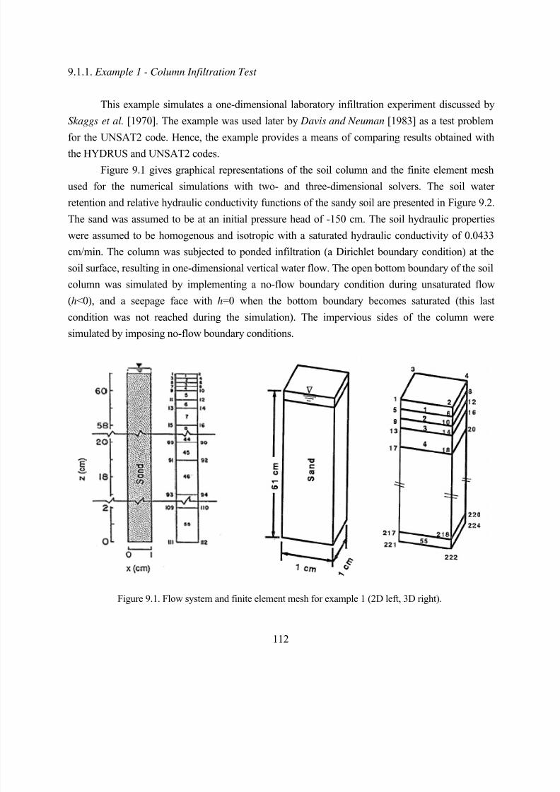
8/20/2019 HYDRUS3D Technical Manual.pdf
http://slidepdf.com/reader/full/hydrus3d-technical-manualpdf 142/260
112
9.1.1. Example 1 - Column Infiltration Test
This example simulates a one-dimensional laboratory infiltration experiment discussed by
Skaggs et al. [1970]. The example was used later by Davis and Neuman [1983] as a test problem
for the UNSAT2 code. Hence, the example provides a means of comparing results obtained withthe HYDRUS and UNSAT2 codes.
Figure 9.1 gives graphical representations of the soil column and the finite element mesh
used for the numerical simulations with two- and three-dimensional solvers. The soil water
retention and relative hydraulic conductivity functions of the sandy soil are presented in Figure 9.2.
The sand was assumed to be at an initial pressure head of -150 cm. The soil hydraulic properties
were assumed to be homogenous and isotropic with a saturated hydraulic conductivity of 0.0433
cm/min. The column was subjected to ponded infiltration (a Dirichlet boundary condition) at the
soil surface, resulting in one-dimensional vertical water flow. The open bottom boundary of the soil
column was simulated by implementing a no-flow boundary condition during unsaturated flow
(h<0), and a seepage face with h=0 when the bottom boundary becomes saturated (this last
condition was not reached during the simulation). The impervious sides of the column were
simulated by imposing no-flow boundary conditions.
Figure 9.1. Flow system and finite element mesh for example 1 (2D left, 3D right).
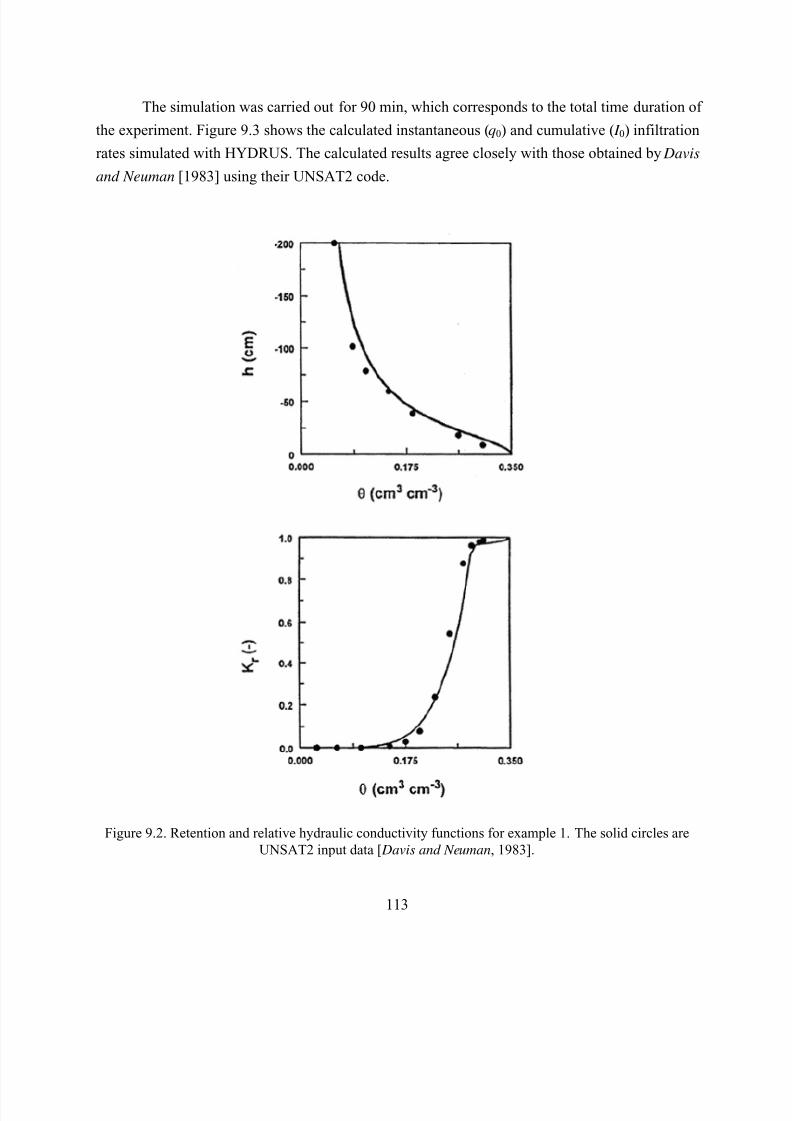
8/20/2019 HYDRUS3D Technical Manual.pdf
http://slidepdf.com/reader/full/hydrus3d-technical-manualpdf 143/260
113
The simulation was carried out for 90 min, which corresponds to the total time duration of
the experiment. Figure 9.3 shows the calculated instantaneous (q0) and cumulative ( I 0) infiltration
rates simulated with HYDRUS. The calculated results agree closely with those obtained by Davis
and Neuman [1983] using their UNSAT2 code.
Figure 9.2. Retention and relative hydraulic conductivity functions for example 1. The solid circles areUNSAT2 input data [ Davis and Neuman, 1983].
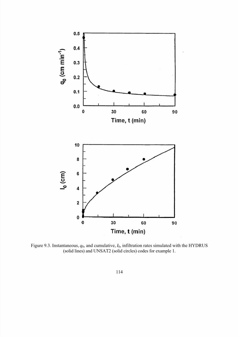
8/20/2019 HYDRUS3D Technical Manual.pdf
http://slidepdf.com/reader/full/hydrus3d-technical-manualpdf 144/260
114
Figure 9.3. Instantaneous, q0, and cumulative, I 0, infiltration rates simulated with the HYDRUS(solid lines) and UNSAT2 (solid circles) codes for example 1.
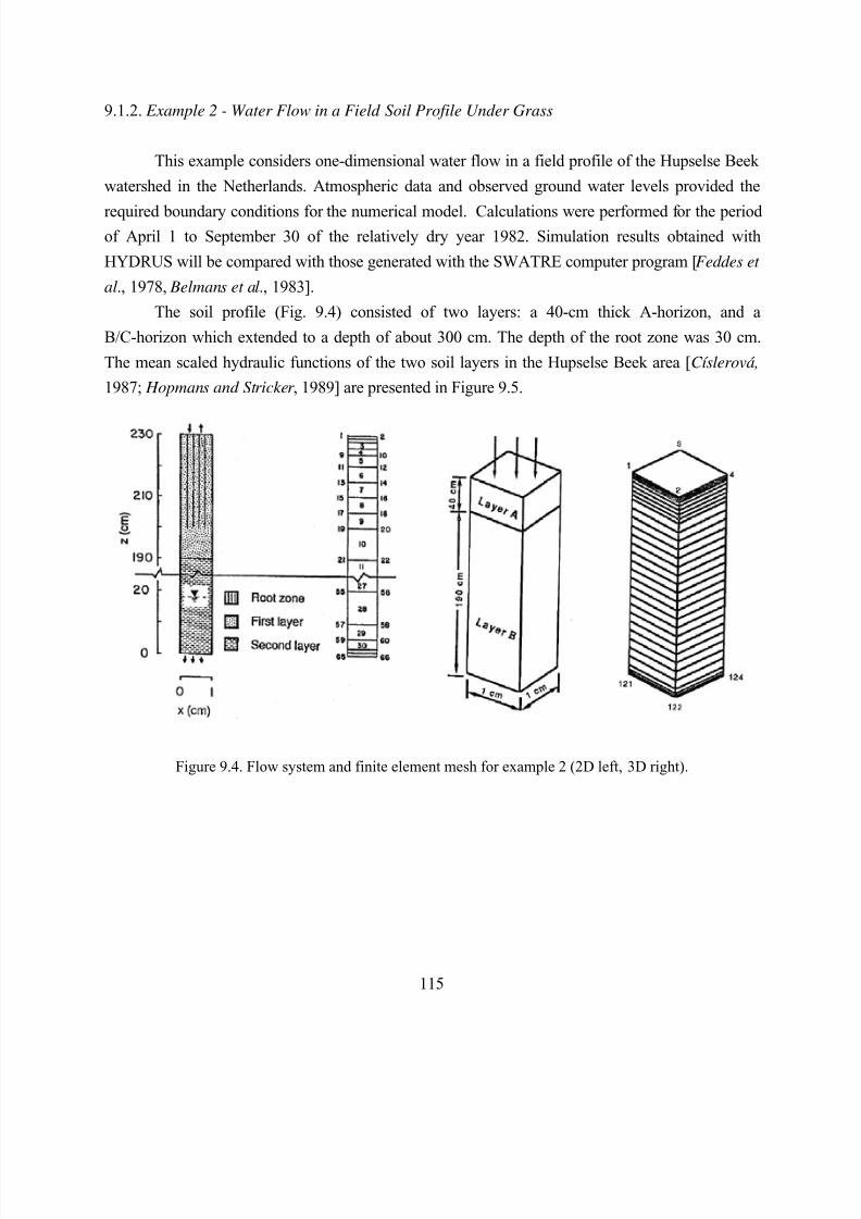
8/20/2019 HYDRUS3D Technical Manual.pdf
http://slidepdf.com/reader/full/hydrus3d-technical-manualpdf 145/260
115
9.1.2. Example 2 - Water Flow in a Field Soil Profile Under Grass
This example considers one-dimensional water flow in a field profile of the Hupselse Beek
watershed in the Netherlands. Atmospheric data and observed ground water levels provided the
required boundary conditions for the numerical model. Calculations were performed for the periodof April 1 to September 30 of the relatively dry year 1982. Simulation results obtained with
HYDRUS will be compared with those generated with the SWATRE computer program [Feddes et
al., 1978, Belmans et al., 1983].
The soil profile (Fig. 9.4) consisted of two layers: a 40-cm thick A-horizon, and a
B/C-horizon which extended to a depth of about 300 cm. The depth of the root zone was 30 cm.
The mean scaled hydraulic functions of the two soil layers in the Hupselse Beek area [ Císlerová,
1987; Hopmans and Stricker , 1989] are presented in Figure 9.5.
Figure 9.4. Flow system and finite element mesh for example 2 (2D left, 3D right).
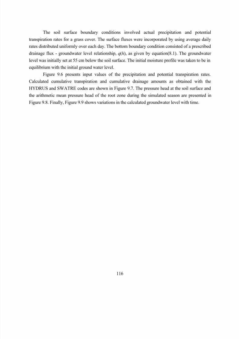
8/20/2019 HYDRUS3D Technical Manual.pdf
http://slidepdf.com/reader/full/hydrus3d-technical-manualpdf 146/260
116
The soil surface boundary conditions involved actual precipitation and potential
transpiration rates for a grass cover. The surface fluxes were incorporated by using average daily
rates distributed uniformly over each day. The bottom boundary condition consisted of a prescribed
drainage flux - groundwater level relationship, q(h), as given by equation(8.1). The groundwater
level was initially set at 55 cm below the soil surface. The initial moisture profile was taken to be inequilibrium with the initial ground water level.
Figure 9.6 presents input values of the precipitation and potential transpiration rates.
Calculated cumulative transpiration and cumulative drainage amounts as obtained with the
HYDRUS and SWATRE codes are shown in Figure 9.7. The pressure head at the soil surface and
the arithmetic mean pressure head of the root zone during the simulated season are presented in
Figure 9.8. Finally, Figure 9.9 shows variations in the calculated groundwater level with time.
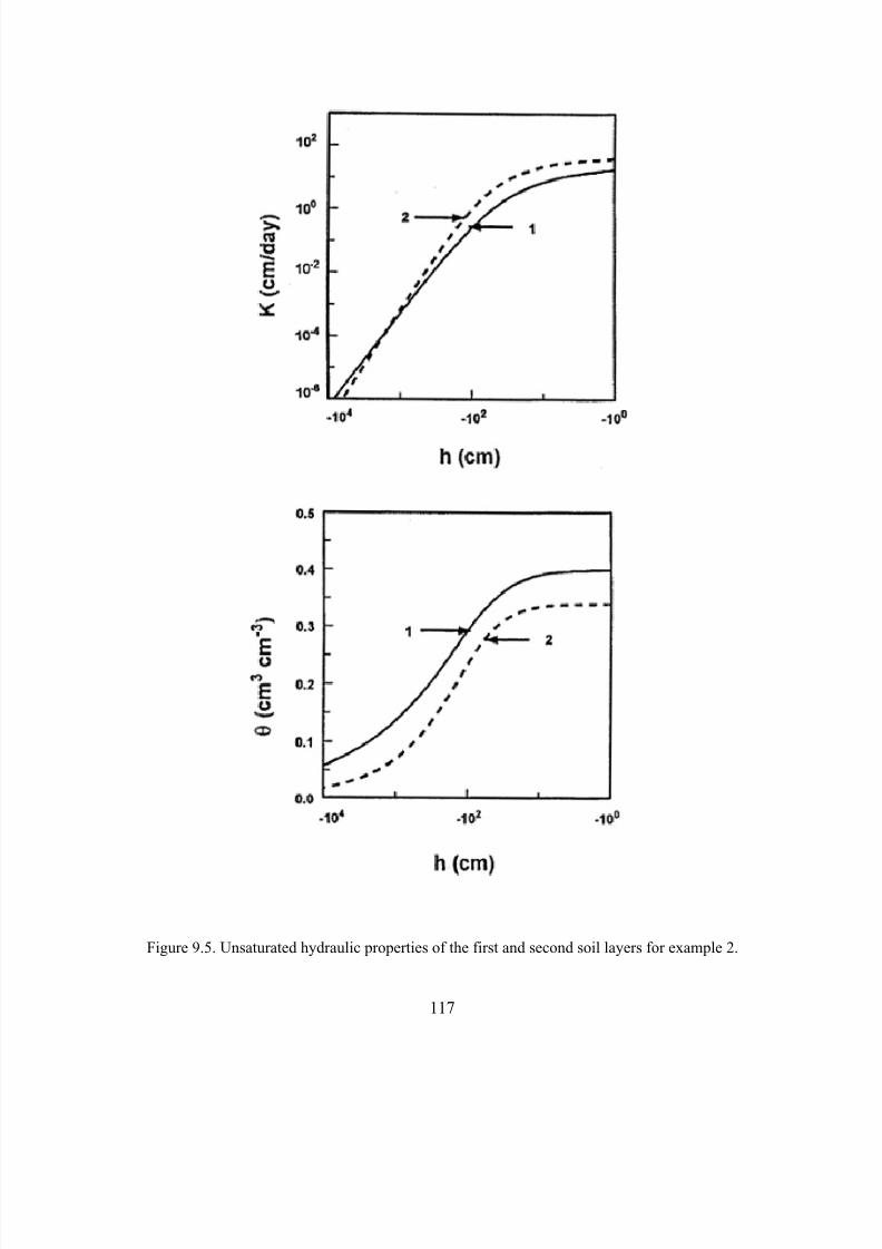
8/20/2019 HYDRUS3D Technical Manual.pdf
http://slidepdf.com/reader/full/hydrus3d-technical-manualpdf 147/260
117
Figure 9.5. Unsaturated hydraulic properties of the first and second soil layers for example 2.
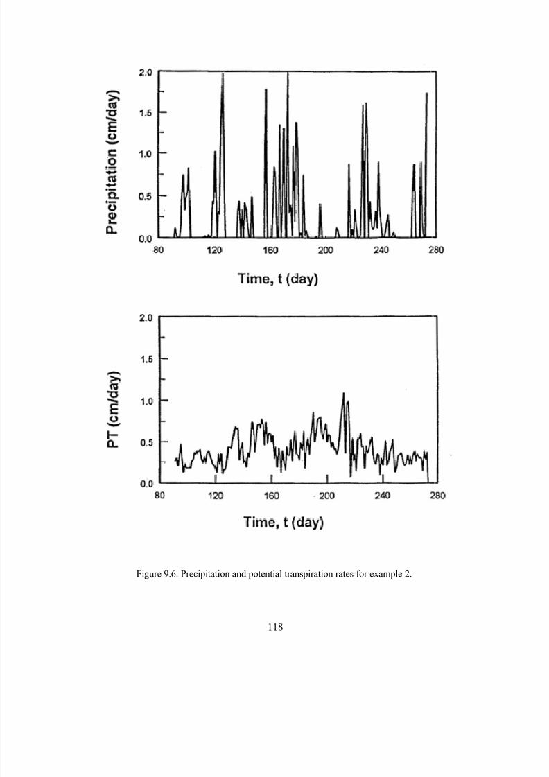
8/20/2019 HYDRUS3D Technical Manual.pdf
http://slidepdf.com/reader/full/hydrus3d-technical-manualpdf 148/260
118
Figure 9.6. Precipitation and potential transpiration rates for example 2.
8/20/2019 HYDRUS3D Technical Manual.pdf
http://slidepdf.com/reader/full/hydrus3d-technical-manualpdf 149/260
119
Figure 9.7. Cumulative values for the actual transpiration and bottom discharge rates for example 2 assimulated with HYDRUS (solid line) and SWATRE (solid circles).
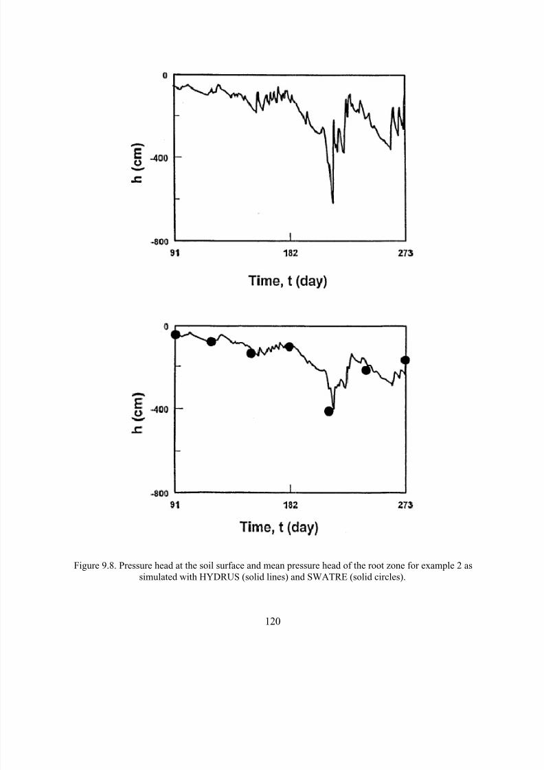
8/20/2019 HYDRUS3D Technical Manual.pdf
http://slidepdf.com/reader/full/hydrus3d-technical-manualpdf 150/260
120
Figure 9.8. Pressure head at the soil surface and mean pressure head of the root zone for example 2 assimulated with HYDRUS (solid lines) and SWATRE (solid circles).
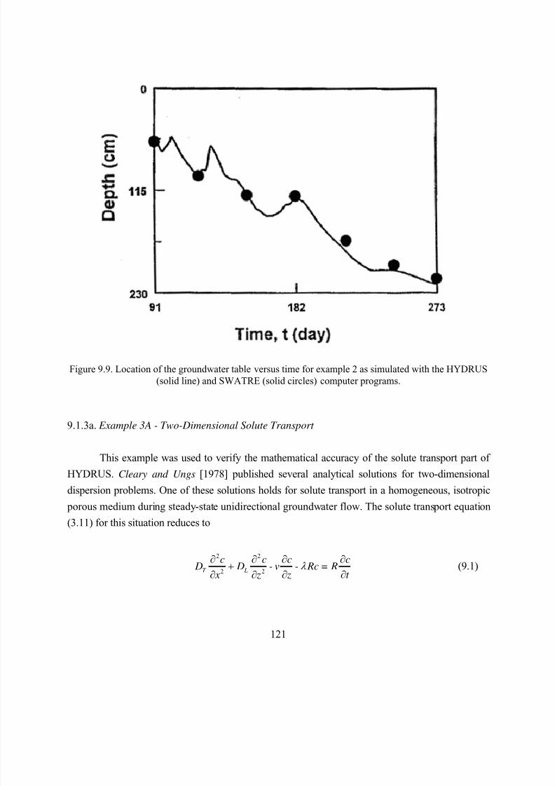
8/20/2019 HYDRUS3D Technical Manual.pdf
http://slidepdf.com/reader/full/hydrus3d-technical-manualpdf 151/260
121
Figure 9.9. Location of the groundwater table versus time for example 2 as simulated with the HYDRUS(solid line) and SWATRE (solid circles) computer programs.
9.1.3a. Example 3A - Two-Dimensional Solute Transport
This example was used to verify the mathematical accuracy of the solute transport part of
HYDRUS. Cleary and Ungs [1978] published several analytical solutions for two-dimensional
dispersion problems. One of these solutions holds for solute transport in a homogeneous, isotropic
porous medium during steady-state unidirectional groundwater flow. The solute transport equation
(3.11) for this situation reduces to
2 2
2 2T L
c c c c D D - v - Rc = R
z t x z λ
∂ ∂ ∂ ∂+
∂ ∂∂ ∂ (9.1)
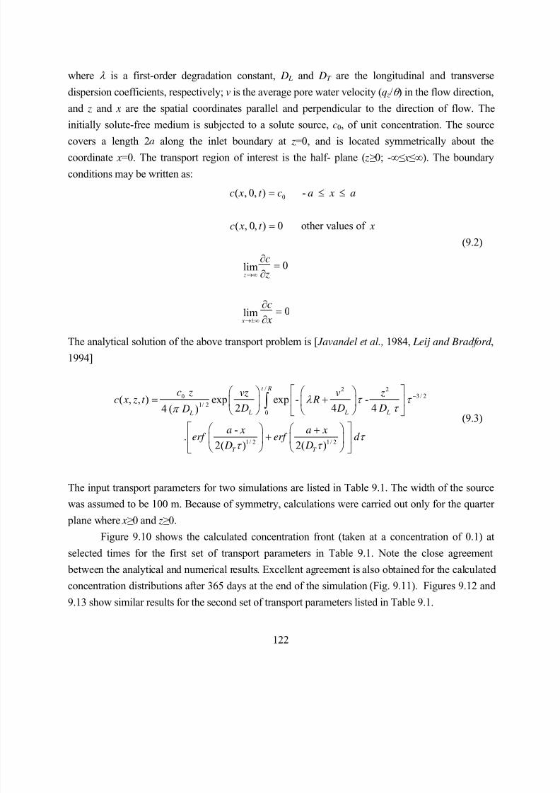
8/20/2019 HYDRUS3D Technical Manual.pdf
http://slidepdf.com/reader/full/hydrus3d-technical-manualpdf 152/260
122
where λ is a first-order degradation constant, D L and DT are the longitudinal and transverse
dispersion coefficients, respectively; v is the average pore water velocity (q z/θ ) in the flow direction,
and z and x are the spatial coordinates parallel and perpendicular to the direction of flow. The
initially solute-free medium is subjected to a solute source, c0, of unit concentration. The source
covers a length 2a along the inlet boundary at z=0, and is located symmetrically about thecoordinate x=0. The transport region of interest is the half- plane ( z≥ 0; -∞≤ x≤∞). The boundary
conditions may be written as:
0( , 0, ) -
( , 0, ) 0 other values of
0lim
0lim
z
x
c x t c a x a
c x t x
c
z
c
x
→∞
→±∞
= ≤ ≤
=
∂=
∂
∂=
∂
(9.2)
The analytical solution of the above transport problem is [ Javandel et al., 1984, Leij and Bradford ,
1994]
/ 2 23 / 20
1/ 20
1/ 2 1/ 2
( , , ) exp exp - -2 4 44 ( )
-.
2( ) 2( )
t R
L L L L
T T
c z vz v zc x z t R
D D D D
a x a xerf erf d
D D
λ τ τ τ π
τ τ τ
−
= +
++
∫ (9.3)
The input transport parameters for two simulations are listed in Table 9.1. The width of the source
was assumed to be 100 m. Because of symmetry, calculations were carried out only for the quarter
plane where x≥ 0 and z≥ 0.
Figure 9.10 shows the calculated concentration front (taken at a concentration of 0.1) at
selected times for the first set of transport parameters in Table 9.1. Note the close agreement between the analytical and numerical results. Excellent agreement is also obtained for the calculated
concentration distributions after 365 days at the end of the simulation (Fig. 9.11). Figures 9.12 and
9.13 show similar results for the second set of transport parameters listed in Table 9.1.
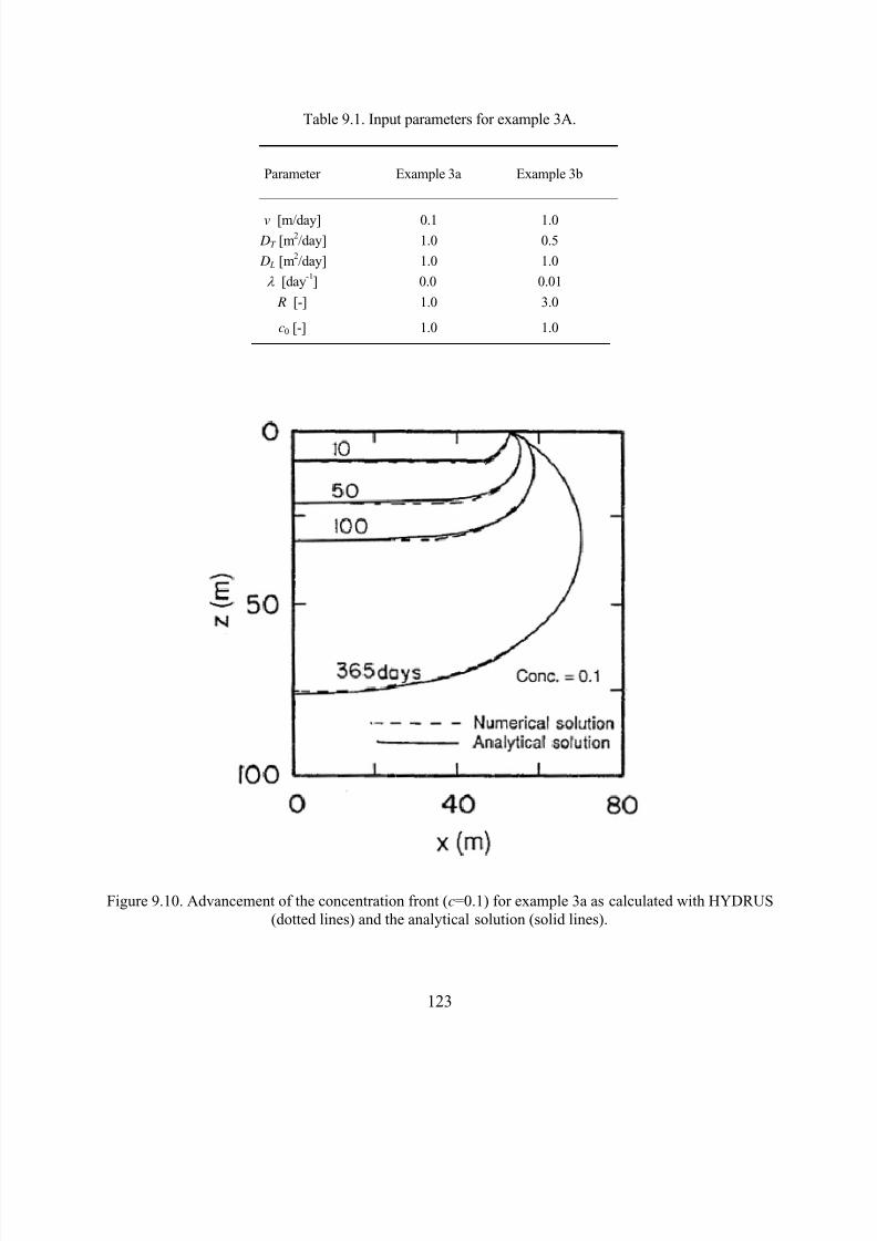
8/20/2019 HYDRUS3D Technical Manual.pdf
http://slidepdf.com/reader/full/hydrus3d-technical-manualpdf 153/260
123
Table 9.1. Input parameters for example 3A.
Parameter Example 3a Example 3b
v [m/day] 0.1 1.0 DT [m
2/day] 1.0 0.5
D L [m2/day] 1.0 1.0
λ [day-1] 0.0 0.01
R [-] 1.0 3.0
c0 [-] 1.0 1.0
Figure 9.10. Advancement of the concentration front (c=0.1) for example 3a as calculated with HYDRUS(dotted lines) and the analytical solution (solid lines).
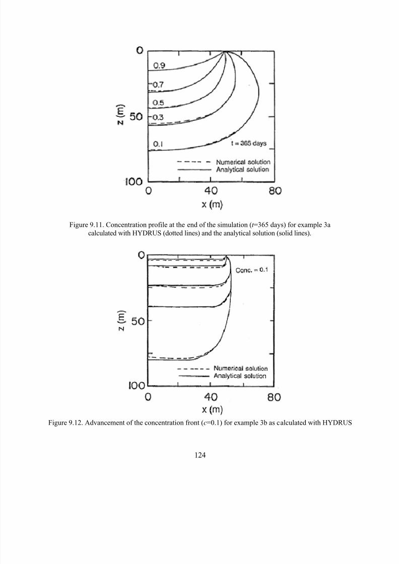
8/20/2019 HYDRUS3D Technical Manual.pdf
http://slidepdf.com/reader/full/hydrus3d-technical-manualpdf 154/260
124
Figure 9.11. Concentration profile at the end of the simulation (t =365 days) for example 3acalculated with HYDRUS (dotted lines) and the analytical solution (solid lines).
Figure 9.12. Advancement of the concentration front (c=0.1) for example 3b as calculated with HYDRUS
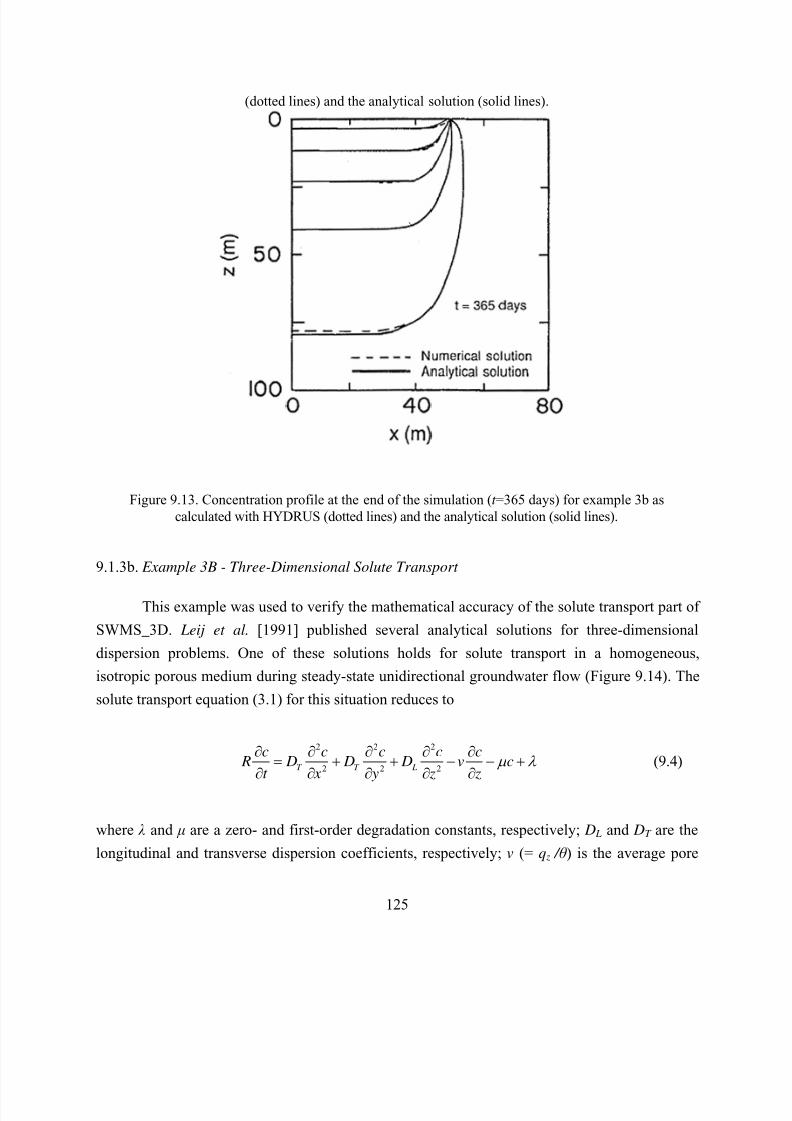
8/20/2019 HYDRUS3D Technical Manual.pdf
http://slidepdf.com/reader/full/hydrus3d-technical-manualpdf 155/260
125
(dotted lines) and the analytical solution (solid lines).
Figure 9.13. Concentration profile at the end of the simulation (t =365 days) for example 3b ascalculated with HYDRUS (dotted lines) and the analytical solution (solid lines).
9.1.3b. Example 3B - Three-Dimensional Solute Transport
This example was used to verify the mathematical accuracy of the solute transport part of
SWMS_3D. Leij et al. [1991] published several analytical solutions for three-dimensional
dispersion problems. One of these solutions holds for solute transport in a homogeneous,
isotropic porous medium during steady-state unidirectional groundwater flow (Figure 9.14). The
solute transport equation (3.1) for this situation reduces to
2 2 2
2 2 2T T L
c c c c c R D D D v c
t x y z zµ λ
∂ ∂ ∂ ∂ ∂= + + − − +
∂ ∂ ∂ ∂ ∂ (9.4)
where λ and μ are a zero- and first-order degradation constants, respectively; D L and DT are the
longitudinal and transverse dispersion coefficients, respectively; v (= q z / θ ) is the average pore
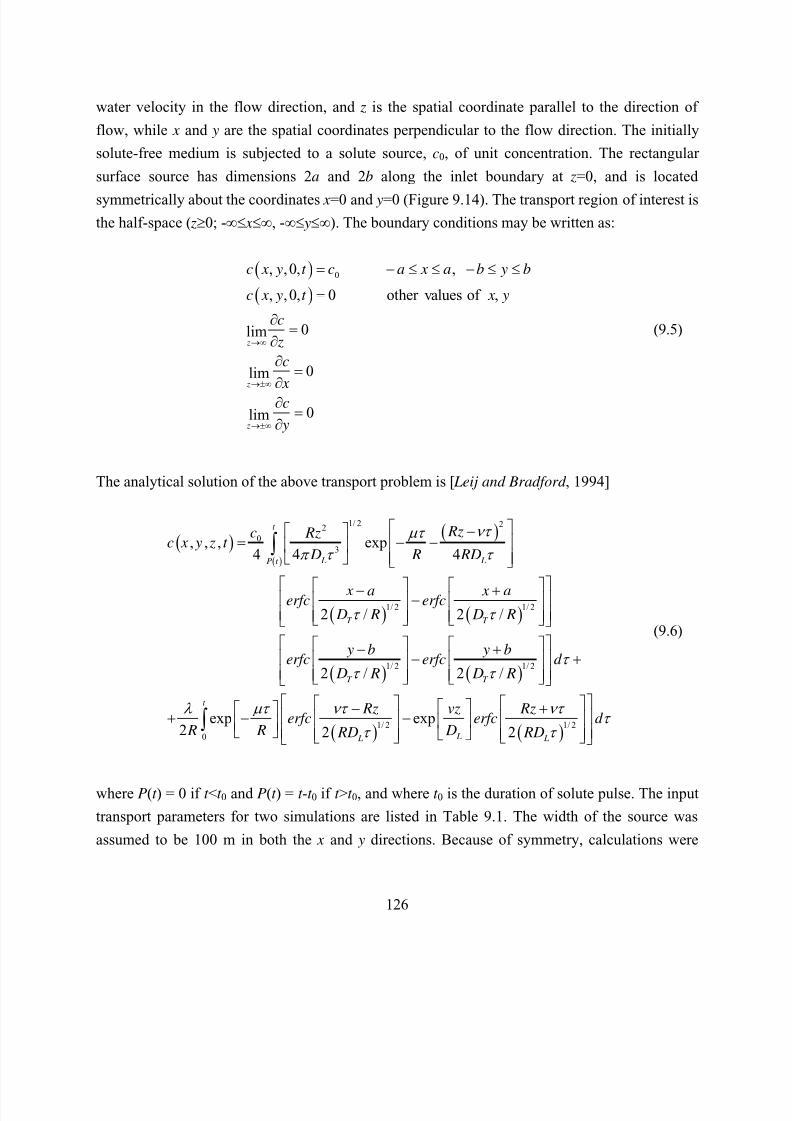
8/20/2019 HYDRUS3D Technical Manual.pdf
http://slidepdf.com/reader/full/hydrus3d-technical-manualpdf 156/260
126
water velocity in the flow direction, and z is the spatial coordinate parallel to the direction of
flow, while x and y are the spatial coordinates perpendicular to the flow direction. The initially
solute-free medium is subjected to a solute source, c0, of unit concentration. The rectangular
surface source has dimensions 2a and 2b along the inlet boundary at z=0, and is located
symmetrically about the coordinates x=0 and y=0 (Figure 9.14). The transport region of interest isthe half-space ( z≥0; -∞≤ x≤∞, -∞≤ y≤∞). The boundary conditions may be written as:
( )
( )0, ,0, ,
, ,0, 0 other values of ,
0lim
0lim
0lim
z
z
z
c x y t c a x a b y b
c x y t x y
c
z
c
x
c
y
→∞
→±∞
→±∞
= − ≤ ≤ − ≤ ≤
=
∂=
∂∂
=∂∂
=∂
(9.5)
The analytical solution of the above transport problem is [ Leij and Bradford , 1994]
( ) ( )
( )
( ) ( )
( ) ( )
1/ 2 220
3
1/ 2 1/ 2
1/ 2 1/ 2
, , , exp4 4 4
2 / 2 /
2 / 2 /
exp2
t
L LP t
T T
T T
Rzc Rzc x y z t
D R RD
x a x aerfc erfc D R D R
y b y berfc erfc d
D R D R
erfc R R
ντ µτ
π τ τ
τ τ
τ τ τ
λ µτ ν
− = − −
− + −
− + − +
+ −
∫
( ) ( )1/ 2 1/ 2
0
exp2 2
t
L L L
Rz vz Rzerfc d
D RD RD
τ ντ τ
τ τ
− + −
∫
(9.6)
where P(t ) = 0 if t <t 0 and P(t ) = t -t 0 if t >t 0, and where t 0 is the duration of solute pulse. The input
transport parameters for two simulations are listed in Table 9.1. The width of the source was
assumed to be 100 m in both the x and y directions. Because of symmetry, calculations were
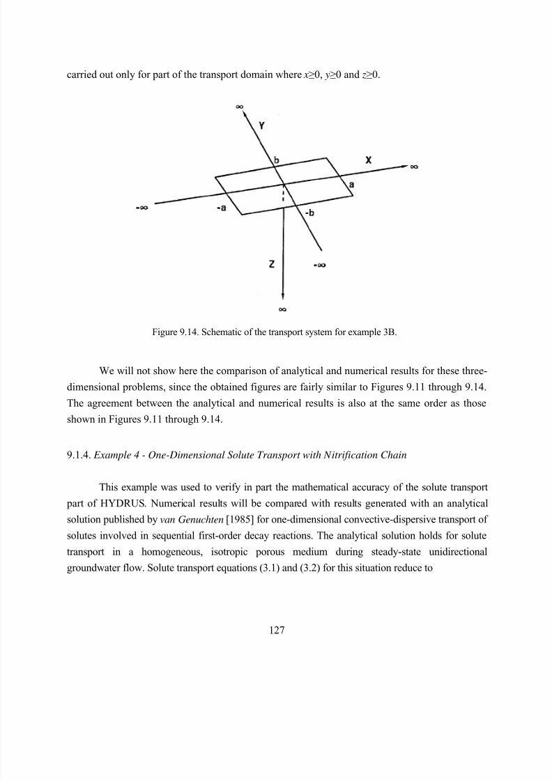
8/20/2019 HYDRUS3D Technical Manual.pdf
http://slidepdf.com/reader/full/hydrus3d-technical-manualpdf 157/260
127
carried out only for part of the transport domain where x≥0, y≥0 and z≥0.
Figure 9.14. Schematic of the transport system for example 3B.
We will not show here the comparison of analytical and numerical results for these three-
dimensional problems, since the obtained figures are fairly similar to Figures 9.11 through 9.14.
The agreement between the analytical and numerical results is also at the same order as those
shown in Figures 9.11 through 9.14.
9.1.4. Example 4 - One-Dimensional Solute Transport with Nitrification Chain
This example was used to verify in part the mathematical accuracy of the solute transport
part of HYDRUS. Numerical results will be compared with results generated with an analytical
solution published by van Genuchten [1985] for one-dimensional convective-dispersive transport of
solutes involved in sequential first-order decay reactions. The analytical solution holds for solute
transport in a homogeneous, isotropic porous medium during steady-state unidirectionalgroundwater flow. Solute transport equations (3.1) and (3.2) for this situation reduce to
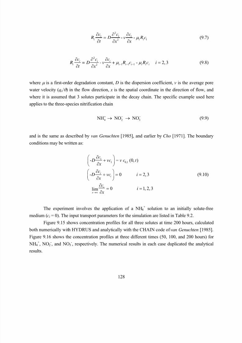
8/20/2019 HYDRUS3D Technical Manual.pdf
http://slidepdf.com/reader/full/hydrus3d-technical-manualpdf 158/260
128
21 1 1
1 1 1 12- -
c c c R D v R c
t x x µ
∂ ∂ ∂=
∂ ∂∂ (9.7)
2
1 1 12- 2, 3i i i
i i i i i i ic c c R = D - v + R c R c it x x
µ µ − − −∂ ∂ ∂ =∂ ∂∂
(9.8)
where µ is a first-order degradation constant, D is the dispersion coefficient, v is the average pore
water velocity (q x/θ ) in the flow direction, x is the spatial coordinate in the direction of flow, and
where it is assumed that 3 solutes participate in the decay chain. The specific example used here
applies to the three-species nitrification chain
4 2 3 NH NO NO
+ − −
→ → (9.9)
and is the same as described by van Genuchten [1985], and earlier by Cho [1971]. The boundary
conditions may be written as:
11 0,1- (0, )
- 0 2, 3
0 1, 2, 3lim
i
i
i
x
c D vc v c t
x
c D vc i
xc
i x→∞
∂ + = ∂
∂ + = =
∂ ∂= =
∂
(9.10)
The experiment involves the application of a NH4+ solution to an initially solute-free
medium (ci = 0). The input transport parameters for the simulation are listed in Table 9.2.
Figure 9.15 shows concentration profiles for all three solutes at time 200 hours, calculated
both numerically with HYDRUS and analytically with the CHAIN code of van Genuchten [1985].
Figure 9.16 shows the concentration profiles at three different times (50, 100, and 200 hours) for
NH4+, NO2
-, and NO3-, respectively. The numerical results in each case duplicated the analytical
results.
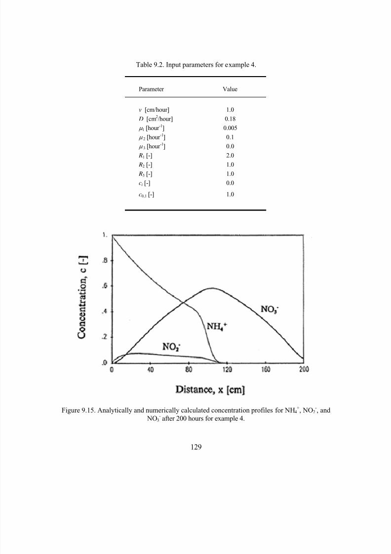
8/20/2019 HYDRUS3D Technical Manual.pdf
http://slidepdf.com/reader/full/hydrus3d-technical-manualpdf 159/260
8/20/2019 HYDRUS3D Technical Manual.pdf
http://slidepdf.com/reader/full/hydrus3d-technical-manualpdf 160/260
130
Figure 9.16. Analytically and numerically calculated concentration profiles for NH4+ (top), NO2
- (middle), NO3
- (bottom) after 50, 100, and 200 hours for example 4.
8/20/2019 HYDRUS3D Technical Manual.pdf
http://slidepdf.com/reader/full/hydrus3d-technical-manualpdf 161/260
131
9.1.5. Example 5 - One-Dimensional Solute Transport with Nonlinear Cation Adsorption
The experiment discussed in this example was conducted by Selim et al. [1987], and used
later for validation of the HYDRUS code [Kool and van Genuchten, 1991]. The soil in this
experiment was Abist loam. A 10.75-cm long soil column was first saturated with a 10 mmolcL-1
CaCl2 solution. The experiment consisted of applying a 14.26 pore volume pulse (t =358.05 hours)
of 10 mmolcL-1 MgCl2 solution, followed by the original CaCl2 solution. The adsorption isotherm
was determined with the help of batch experiments [Selim et al., 1987], and fitted with the
Freundlich equation (3.3) [Kool and van Genuchten, 1991]. The Freundlich isotherm parameters, as
well as other transport parameters for this problem, are listed in Table 9.3. First- and second-type
boundary conditions were applied at the top and bottom of the soil column, respectively.
The observed Mg breakthrough curve is shown in Figure 9.17, together with simulated
breakthrough curves obtained with HYDRUS, the MONOC code of Selim et al. [1987] and the
version 3.1 of the HYDRUS code of Kool and van Genuchten [1991]. The results indicate a
reasonable prediction of the measured breakthrough curve using HYDRUS, and close
correspondence between the simulated results obtained with the HYDRUS and MONOC models.
The HYDRUS results became identical to those generated with HYDRUS-3.1 when a third-type
boundary condition was invoked at the top of the soil column.
Table 9.3. Input parameters for example 5.
Parameter Value
q [cm/hour] 0.271
D [cm2/hour] 1.167
ρ [g/cm3] 0.884
θ [-] 0.633
c0 [mmolc/L] 10.0
k s [cm3/g] 1.687
β [-] 1.615
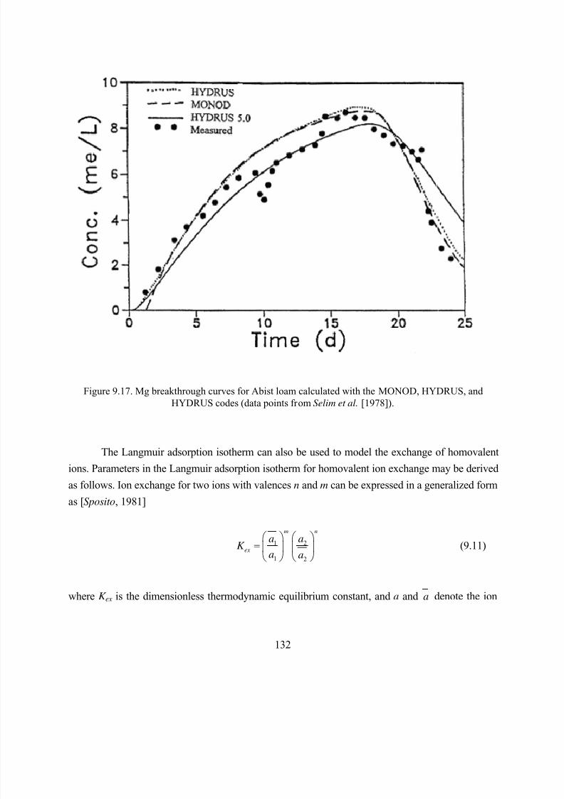
8/20/2019 HYDRUS3D Technical Manual.pdf
http://slidepdf.com/reader/full/hydrus3d-technical-manualpdf 162/260
132
Figure 9.17. Mg breakthrough curves for Abist loam calculated with the MONOD, HYDRUS, andHYDRUS codes (data points from Selim et al. [1978]).
The Langmuir adsorption isotherm can also be used to model the exchange of homovalent
ions. Parameters in the Langmuir adsorption isotherm for homovalent ion exchange may be derived
as follows. Ion exchange for two ions with valences n and m can be expressed in a generalized form
as [Sposito, 1981]
1 2
1 2
m n
ex
a aK
aa
=
(9.11)
where K ex is the dimensionless thermodynamic equilibrium constant, and a and a denote the ion
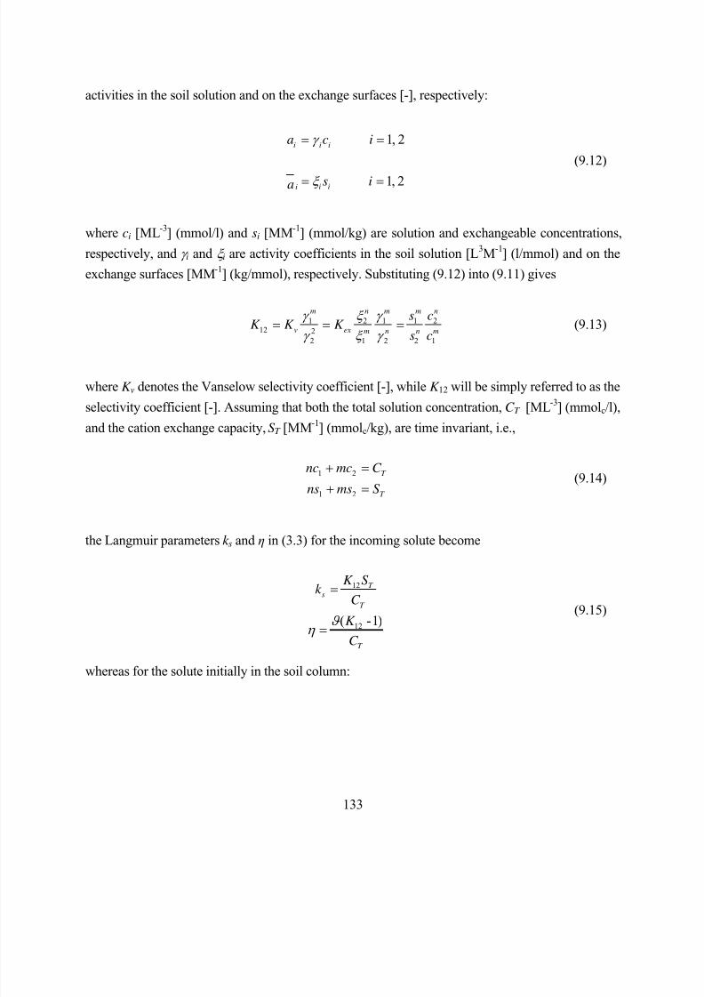
8/20/2019 HYDRUS3D Technical Manual.pdf
http://slidepdf.com/reader/full/hydrus3d-technical-manualpdf 163/260
133
activities in the soil solution and on the exchange surfaces [-], respectively:
1, 2
1, 2
i i i
i ii
a c i
s ia
γ
ξ
= =
= =
(9.12)
where ci [ML-3] (mmol/l) and si [MM-1] (mmol/kg) are solution and exchangeable concentrations,
respectively, and γ i and ξ i are activity coefficients in the soil solution [L3M-1] (l/mmol) and on the
exchange surfaces [MM-1] (kg/mmol), respectively. Substituting (9.12) into (9.11) gives
1 2 1 1 212 2
2 1 2 2 1
m n m m n
v ex m n n m
s cK K K
s c
γ ξ γ
γ ξ γ = = = (9.13)
where K v denotes the Vanselow selectivity coefficient [-], while K 12 will be simply referred to as the
selectivity coefficient [-]. Assuming that both the total solution concentration, C T [ML-3] (mmolc/l),
and the cation exchange capacity, S T [MM-1] (mmolc/kg), are time invariant, i.e.,
1 2
1 2
T
T
nc mc C
ns ms S
+ =
+ = (9.14)
the Langmuir parameters k s and η in (3.3) for the incoming solute become
12
12( -1)
T s
T
T
K S k
C
K
C
ϑ η
=
=
(9.15)
whereas for the solute initially in the soil column:
8/20/2019 HYDRUS3D Technical Manual.pdf
http://slidepdf.com/reader/full/hydrus3d-technical-manualpdf 164/260
134
12
12
12
(1- )
T s
T
T
S k
K C
K
K C
ϑ η
=
=
(9.16)
The parameter υ in (9.15) and (9.16) equals 1 for monovalent ions, and 2 for divalent ions.
The selectivity coefficient K 12 for example 5 was measured by Selim et al. [1987]
(K 12=0.51). From the total solution concentration (C T =10 mmolc/l) and the known cation exchange
capacity (S T =62 mmolc/kg), it follows that the parameters in the Langmuir adsorption isotherm for
the incoming solute (Mg) are k s=3.126 and η =-0.098, while those for the solute initially in the soil
profile (Ca) the parameters are k s=12.157 and η =0.192. The observed Ca breakthrough curve is
shown in Figure 9.18, together with the simulated breakthrough curves obtained with the HYDRUS
and MONOC codes [Selim et al., 1987]. Note the close agreement between the numerical resultsand the experimental data.
Figure 9.18. Ca breakthrough curves for Abist loam calculated with the MONOD and HYDRUS codes(data points from Selim et al. [1978]) (example 5).
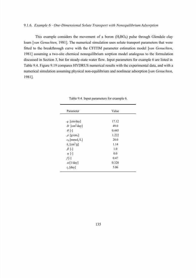
8/20/2019 HYDRUS3D Technical Manual.pdf
http://slidepdf.com/reader/full/hydrus3d-technical-manualpdf 165/260
135
9.1.6. Example 6 - One-Dimensional Solute Transport with Nonequilibrium Adsorption
This example considers the movement of a boron (H3BO4) pulse through Glendale clay
loam [van Genuchten, 1981]. The numerical simulation uses solute transport parameters that were
fitted to the breakthrough curve with the CFITIM parameter estimation model [van Genuchten,1981] assuming a two-site chemical nonequilibrium sorption model analogous to the formulation
discussed in Section 3, but for steady-state water flow. Input parameters for example 6 are listed in
Table 9.4. Figure 9.19 compares HYDRUS numerical results with the experimental data, and with a
numerical simulation assuming physical non-equilibrium and nonlinear adsorption [van Genuchten,
1981].
Table 9.4. Input parameters for example 6.
Parameter Value
q [cm/day] 17.12
D [cm2/day] 49.0
θ [-] 0.445
ρ [g/cm3] 1.222
c0 [mmolc/L] 20.0
k s [cm3/g] 1.14
β [-] 1.0
η [-] 0.0
f [-] 0.47
ω [1/day] 0.320
t p [day] 5.06
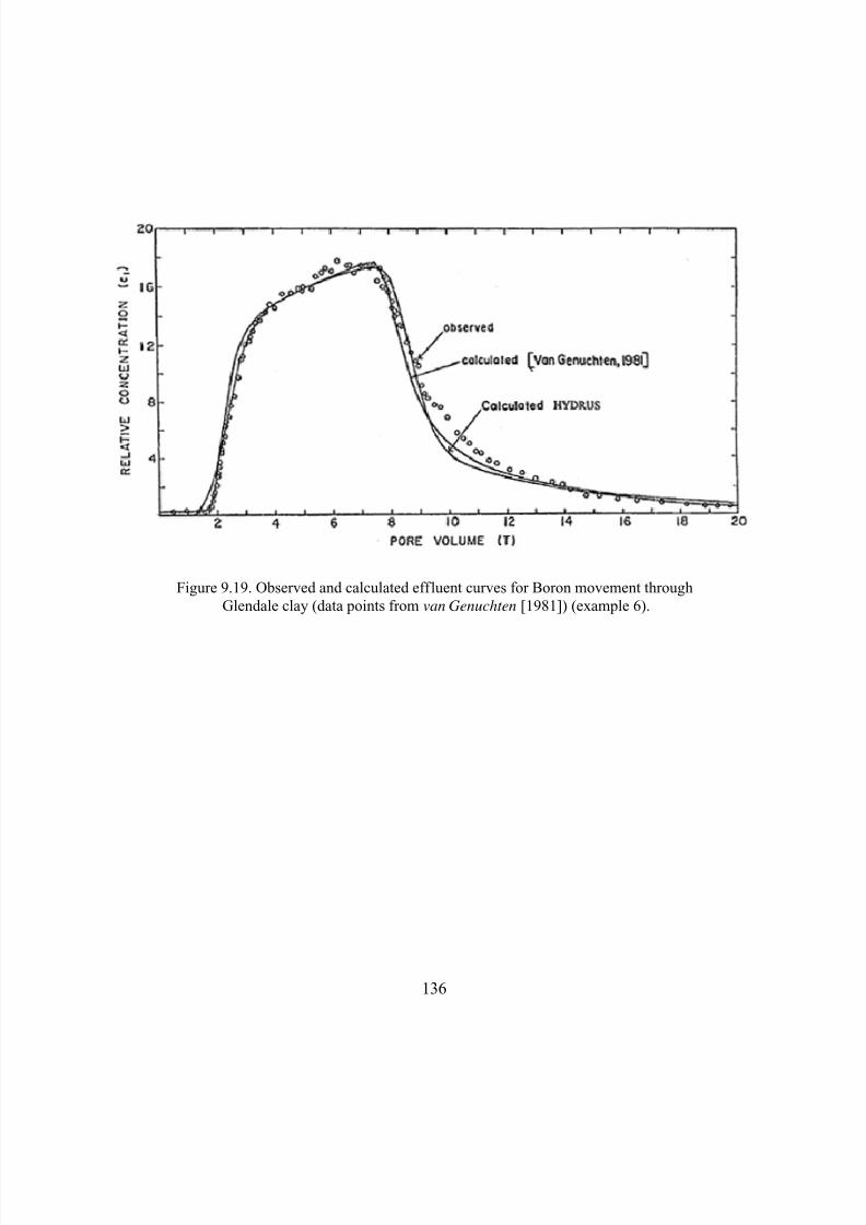
8/20/2019 HYDRUS3D Technical Manual.pdf
http://slidepdf.com/reader/full/hydrus3d-technical-manualpdf 166/260
136
Figure 9.19. Observed and calculated effluent curves for Boron movement throughGlendale clay (data points from van Genuchten [1981]) (example 6).
8/20/2019 HYDRUS3D Technical Manual.pdf
http://slidepdf.com/reader/full/hydrus3d-technical-manualpdf 167/260
137
9.1.7. Example 7 - Water and Solute Infiltration Test
This example corresponds to example 4 in the SWMS_2D and HYDRUS-2D manuals
[Šimůnek et al., 1992, 1999]. The example concerns the movement of water and a dissolved solute
from a single-ring infiltrometer into the soil profile consisting of two layers: a 40-cm thickA-horizon, and an underlying B/C-horizon. The hydraulic functions of the two soil layers are the
same as those used in Example 2. The axisymmetric flow system and associated finite element
mesh for the ponded infiltration experiment are shown in Figure 9.19. The soil profile had an initial
temperature of 20oC, whereas the infiltrated water had a temperature of 30oC and contained an
organic (parent) compound (the pesticide aldicarb) which is known to degrade by oxidation into
two sequential daughter products (sulfone and sulfoxide) [Ou et al., 1988]. Each of the three solutes
also undergoes hydrolytical first-order decay that leads to products which are not simulated or
monitored during their subsequent transport (i.e., oxime, sulfone oxime, and sulfoxide oxime) [Ou
et al., 1988]. All major solutes adsorb onto the solid phase, and volatilization is considered for the
first and the third solutes. The reaction pathway is schematically given by:
Product Product Product
µ l,1↑ µ l,2↑ µ l,3↑ Parent Daughter Daughter
Pesticide µ ' l,1→ Product 1 µ ' l,2→ Product 2 µ ' l,3→ Product
g1 c1 s1 c2 s2 g3 c3 s3 k g,1 k s,1 k s,2 k g,3 k s,3
The example is used here to illustrate variably-saturated water flow, heat movement, and solute
transport in a layered and radially symmetric three-dimensional soil profile.
Calculations were carried out over a period of 10 days. The pressure head profile obtained
in example problem 2 at the beginning of June 1982 was taken as the initial condition for the water
flow equation, similarly as in example 4 of Šimůnek et al. [1992]. The soil profile was assumed to
be initially free of any solutes. All sides of the flow region were considered to be impervious,
except for a small portion around the origin at the surface (the ponded surface inside the ring
infiltrometer) where constant pressure head and concentration flux boundary conditions wereimposed, as well as the lower right corner where the groundwater level was kept constant. The
concentration of the infiltrating water was free of any solute except for the first five days of the
8/20/2019 HYDRUS3D Technical Manual.pdf
http://slidepdf.com/reader/full/hydrus3d-technical-manualpdf 168/260
138
simulation during which time the infiltrating water contained the parent solute of unit
concentration. Boundary condition (3.46) was used for the non-ponded part of the soil surface,
thereby assuming the existence of a stagnant boundary layer of thickness d at the soil surface
through which volatile solutes moved to the atmosphere by gas diffusion only. Water and solute
extraction by plant roots was not considered.Tables 9.5, 9.6, and 9.7 list the unsaturated soil hydraulic, heat and solute transport
parameters, respectively. The solute and heat transport parameters were assumed to be the same for
the two soil layers. The heat transport parameters b1, b2, b3, C n, C o, and C w in Table 9.6 were taken
from Chung and Horton [1987]. The solute parameters k s, k g, µ w, µ w’, and Dg in Table 9.7 were
taken from Wagenet and Hutson [1987].
Figure 9.21 presents the initial and steady-state pressure head profiles. The steady- state
profile for water flow was reached after approximately 2 or 3 days. Temperature profiles at times 1
and 10 days are shown in Figure 9.22. The heat front moved relatively slowly into the soil profile incomparison with the solute front (shown later) because of the high volumetric heat capacity of the
relatively wet soil. Figures 9.23, 9.24, and 9.25 show concentration profiles for all three solutes at
times 2.5, 5, 7.5, and 10 days. After its application in the infiltrating water during the first five days
of the simulation (Fig. 9.23a, b), the first (parent) solute is transported further by water flow and
gaseous diffusion, as well as is being degraded by two first-order decay reactions, such that the soil
profile is practically free of this solute after 10 days (Fig. 9.23c, d). The second solute exists
exclusively because of first-order degradation of the first solute. Hence, the second solute initially
corresponds mainly with the first solute, but subsequently moves faster through the soil profile
because of less sorption. Note that the highest concentrations of the second solute were reachedafter complete application of the first solute (Fig. 9.24c, d). Similar features as for the second solute
also apply to the third solute. In particular, notice that the soil profile is almost free of this solute
after 2.5 days (Fig. 9.25a), and that the highest concentrations of the third solute (while being much
smaller than those for the first two solutes) were reached at the end of the simulation (Fig. 9.25d).
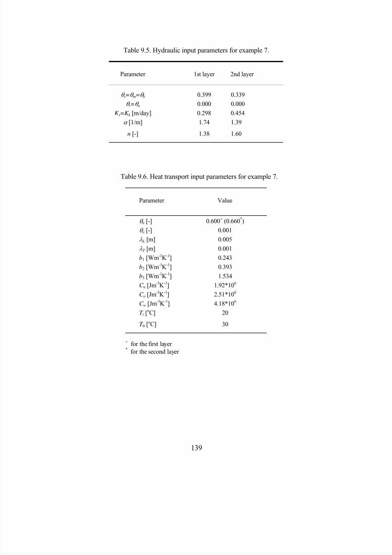
8/20/2019 HYDRUS3D Technical Manual.pdf
http://slidepdf.com/reader/full/hydrus3d-technical-manualpdf 169/260
139
Table 9.5. Hydraulic input parameters for example 7.
Parameter 1st layer 2nd layer
θ s=θ m=θ k 0.399 0.339θ r =θ a 0.000 0.000
K s=K k [m/day] 0.298 0.454
α [1/m] 1.74 1.39
n [-] 1.38 1.60
Table 9.6. Heat transport input parameters for example 7.
Parameter Value
θ n [-] 0.600+ (0.660*)
θ o [-] 0.001
λ L [m] 0.005
λ T [m] 0.001
b1 [Wm-1K -1] 0.243
b2 [Wm-1K -1] 0.393
b3 [Wm-1K -1] 1.534
C n [Jm-3K -1] 1.92*106
C o [Jm-3K -1] 2.51*106 C w [Jm-3K -1] 4.18*106
T i [oC] 20
T 0 [oC] 30
+ for the first layer* for the second layer
8/20/2019 HYDRUS3D Technical Manual.pdf
http://slidepdf.com/reader/full/hydrus3d-technical-manualpdf 170/260
140
Table 9.7. Solute transport input parameters for example 7.
Parameter Value
ρ [kg/m
3
] 1300 Dw [m2/day] 0.00374
Dg [m2/day] 0.432
D L [m] 0.005
DT [m] 0.001
k s,1 [m3/kg] 0.0001
k s,2 [m3/kg] 0.00005
k s,3 [m3/kg] 0.0002
k g,1 [-] 1.33*10-7
k g,2 [-] 0.0
k g,3 [-] 1.33*10-3
µ w,1 [1/day] 0.2µ w,2 [1/day] 0.01
µ w,3 [1/day] 0.005
µ ’w,1 [1/day] 0.36
µ ’w,2 [1/day] 0.024
µ ’w,3 [1/day] 0.0024
c0,1 [-] 1.0
c0,2 [-] 0.0
c0,3 [-] 0.0
d [m] 0.005
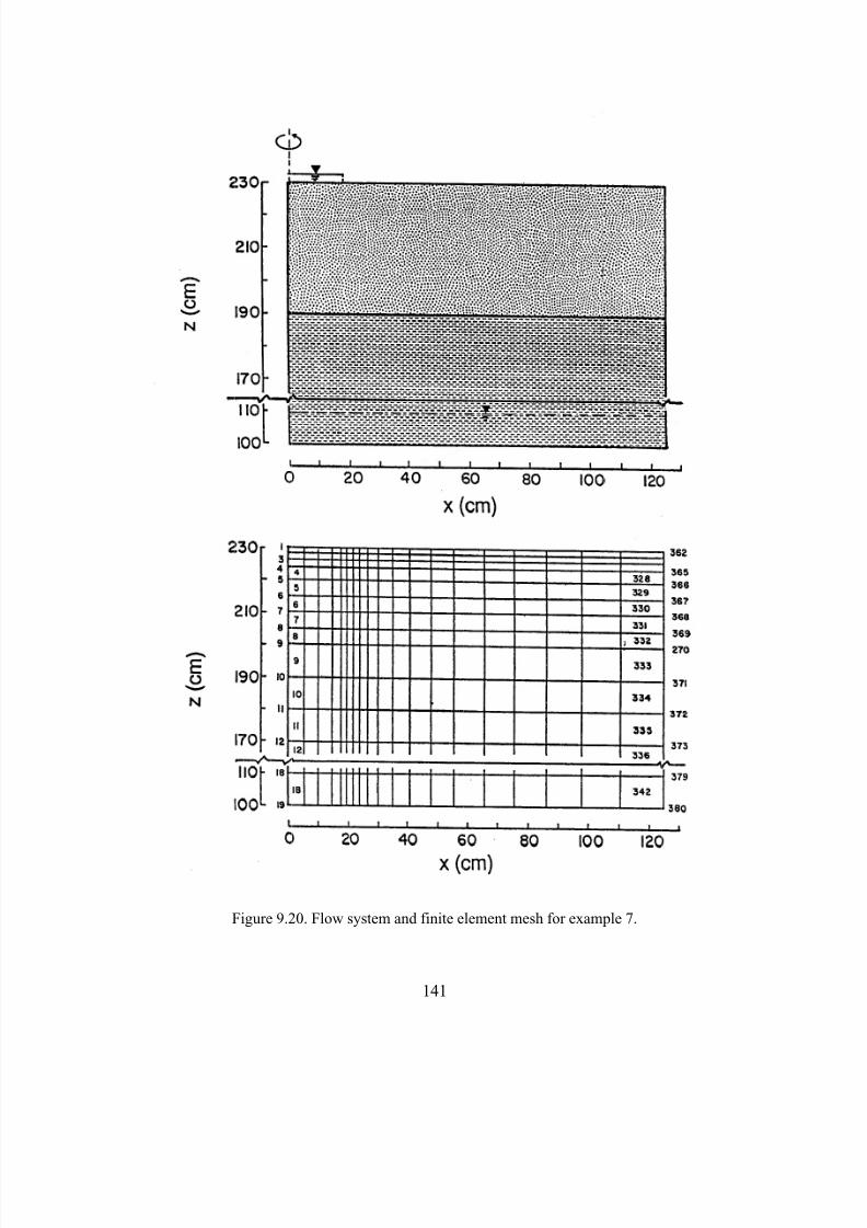
8/20/2019 HYDRUS3D Technical Manual.pdf
http://slidepdf.com/reader/full/hydrus3d-technical-manualpdf 171/260
141
Figure 9.20. Flow system and finite element mesh for example 7.
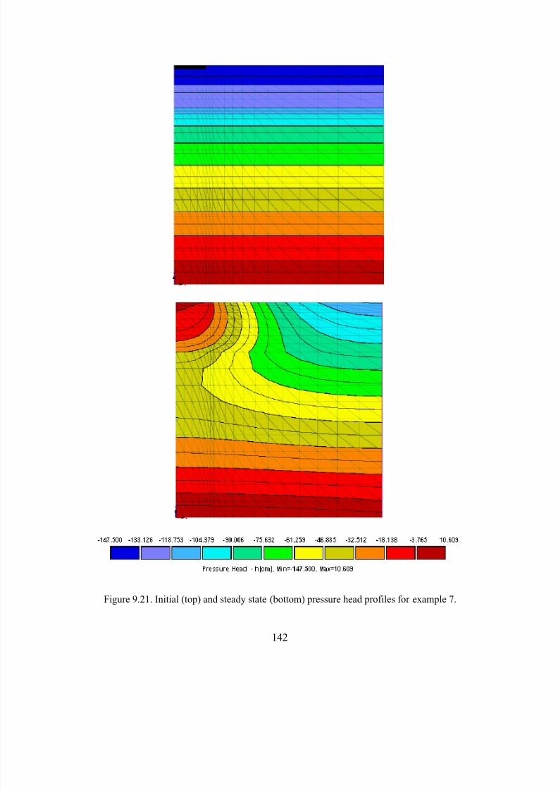
8/20/2019 HYDRUS3D Technical Manual.pdf
http://slidepdf.com/reader/full/hydrus3d-technical-manualpdf 172/260
142
Figure 9.21. Initial (top) and steady state (bottom) pressure head profiles for example 7.
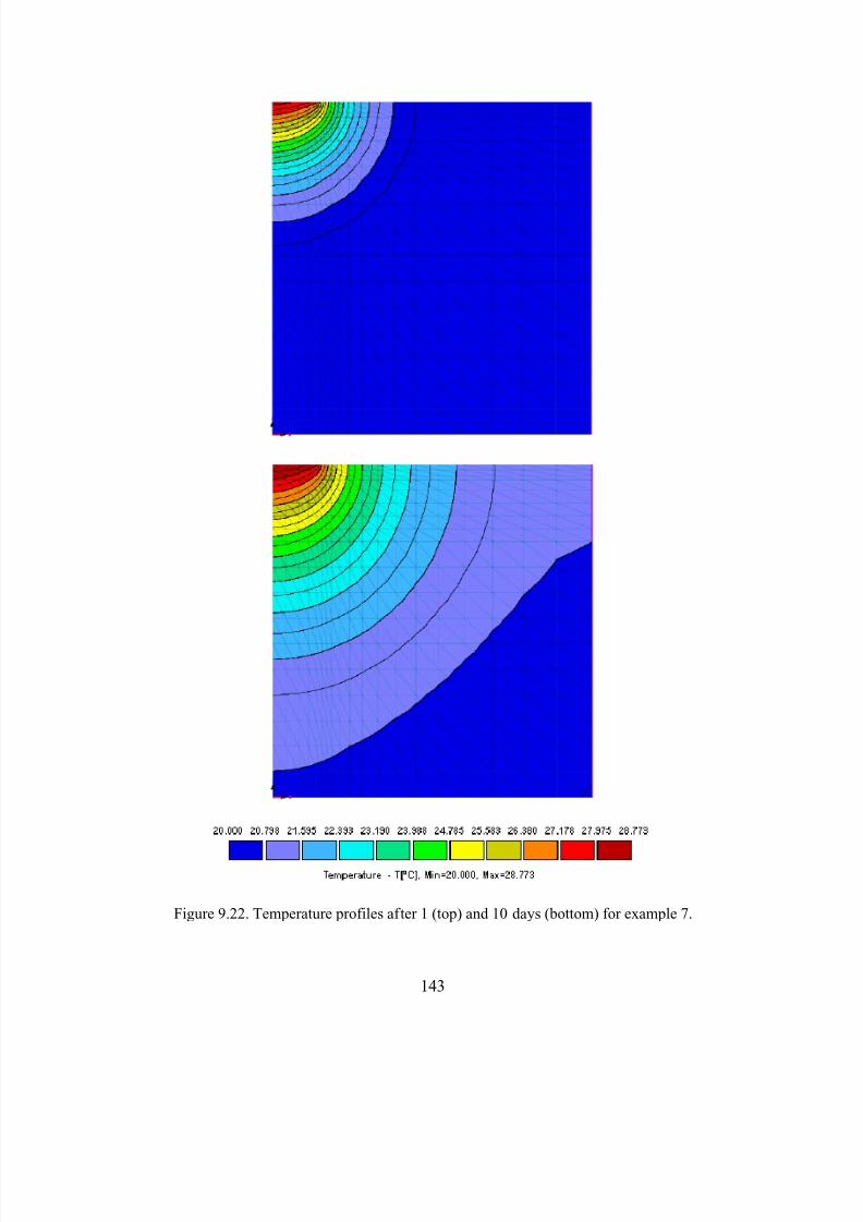
8/20/2019 HYDRUS3D Technical Manual.pdf
http://slidepdf.com/reader/full/hydrus3d-technical-manualpdf 173/260
143
Figure 9.22. Temperature profiles after 1 (top) and 10 days (bottom) for example 7.
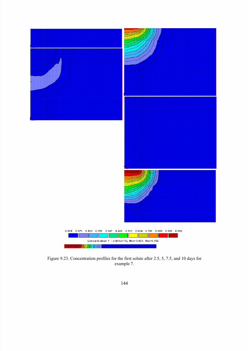
8/20/2019 HYDRUS3D Technical Manual.pdf
http://slidepdf.com/reader/full/hydrus3d-technical-manualpdf 174/260
144
Figure 9.23. Concentration profiles for the first solute after 2.5, 5, 7.5, and 10 days forexample 7.
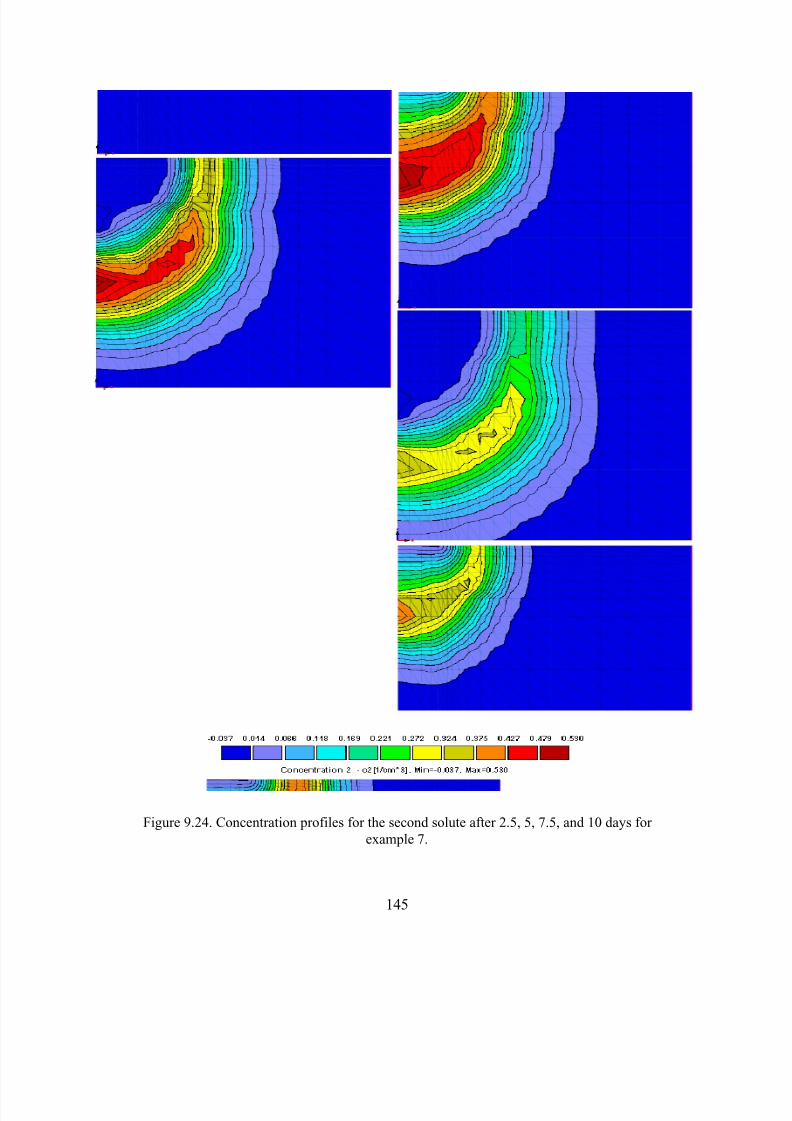
8/20/2019 HYDRUS3D Technical Manual.pdf
http://slidepdf.com/reader/full/hydrus3d-technical-manualpdf 175/260
145
Figure 9.24. Concentration profiles for the second solute after 2.5, 5, 7.5, and 10 days forexample 7.
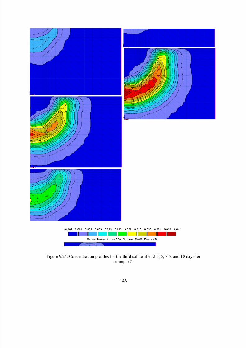
8/20/2019 HYDRUS3D Technical Manual.pdf
http://slidepdf.com/reader/full/hydrus3d-technical-manualpdf 176/260
146
Figure 9.25. Concentration profiles for the third solute after 2.5, 5, 7.5, and 10 days forexample 7.
8/20/2019 HYDRUS3D Technical Manual.pdf
http://slidepdf.com/reader/full/hydrus3d-technical-manualpdf 177/260
147
9.1.8. Example 8 - Contaminant Transport From a Waste Disposal Site
This test problem concerns contaminant transport from a waste disposal site (or possibly
a landfill) into a unconfined aquifer containing a pumping well downgradient of the disposal site
as shown in Figure 9.26. Water was assumed to infiltrate from the disposal site into theunsaturated zone under zero-head ponded conditions. The concentration of the contaminant
leaving the disposal site was taken to be 1.0 during the first 50 days, and zero afterwards. The
waste disposal site itself had lateral dimensions of 10 x 40 m2. Initially, the water table decreased
from a height of 28 m above the base of the aquifer at the left-hand side (Figure 9.26) to 26 m on
the right-hand side of the flow domain. The initial pressure head in the unsaturated zone was
assumed to be at equilibrium with the initial water table, i.e., no vertical flow occurred. The
transport experiment started when the water table in the fully penetrated well at x = 170 m ( y = 0)
was suddenly lowered to a height of 18 m above the bottom of the unconfined aquifer. We
assumed that at that same time (t = 0) infiltration started to occur from the disposal site.
Prescribed hydraulic head conditions h + z = 28 m and h + z = 26 m were imposed along the left-
hand ( x = 0) and right-hand ( x = 260 m) side boundaries (-50≤ y≤50 m). A prescribed hydraulic
head condition of h + z = 18 m was used to represent the well along a vertical below the water
table ( z≤18) at x = 170 m and y = 0 m, while a seepage face was defined at that location along the
vertical above the water table ( z > 18). No-flow conditions were assumed along all other
boundaries, including the soil interface. Hydraulic and transport parameters used in the analysis
are listed in Table 9.8. We selected the retention hydraulic parameters for a coarse-textured soil
with a relatively high saturated hydraulic conductivity, K s, in order to test the HYDRUS code fora comparatively difficult numerical problem.
Because of symmetry about the y axis, only half of the flow region was simulated. The
solution domain defined by 0≤ x≤260, 0≤ y≤50, and 0≤ z≤38 m was discretized into a rectangular
grid comprised of 10560 elements and 12144 nodes (Figure 9.27). Nodal spacings were made
relatively small in regions near the disposal site and near the pumping well where the highest
head gradients and flow velocities were expected. The variably saturated flow problem was
solved using HYDRUS assuming an iteration head tolerance of 0.01 m and a water content
tolerance of 0.0001.
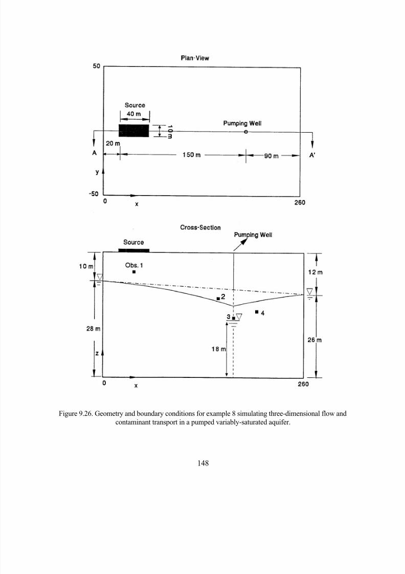
8/20/2019 HYDRUS3D Technical Manual.pdf
http://slidepdf.com/reader/full/hydrus3d-technical-manualpdf 178/260
8/20/2019 HYDRUS3D Technical Manual.pdf
http://slidepdf.com/reader/full/hydrus3d-technical-manualpdf 179/260
149
Table 9.8. Input parameters for example 8.
Hydraulic Parameters Transport Parameters
θ s=θ m=θ k 0.450 ρ [kg/m3
] 1400
θ r =θ a 0.05 Dd [m2/day] 0.01
K s=K k [m/day] 5.0 D L [m] 1.0
α [1/m] 4.1 DT [m] 0.25
n [-] 2.0 k [m3/kg] 0.0
μw [1/day] 0.0
μs [1/day] 0.0
γw [1/day] 0.0
γs [1/day] 0.0
c0 1.0
Computed water table elevations are plotted in Figure 9.28a and 9.28b along longitudinal
( y=0) and transverse ( x=170 m) planes through the pumping well, respectively. The results showa relatively strong direct interaction between the infiltrating water and the saturated zone after
only a short period of time; water flow reached approximately steady state about 1.5 days after
the experiment started. The velocity field and streamlines in a longitudinal section through the
pumping well are presented in Figure 9.29. Note that the length of the seepage face along the
well was determined to be approximately 5 meters. The calculated well discharge rate for the
fixed water table ( z = 18 m) was calculated to be 39.6 m3/day. A concentration contour plot (c =
0.1) is presented in Figure 9.30. This figure shows that contaminant transport was strongly
affected by well pumping. Note that although the contaminant source was located 10 m above the
initial groundwater table, and 150 m upgradient of the pumping well, the solute reached the pumping well after only 200 days of pumping. Figure 9.31 gives a two-dimensional view of
calculated concentration distributions at several times in a horizontal plane ( z = 20 m).
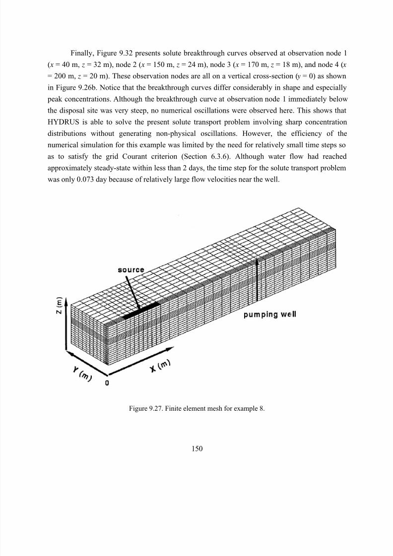
8/20/2019 HYDRUS3D Technical Manual.pdf
http://slidepdf.com/reader/full/hydrus3d-technical-manualpdf 180/260
150
Finally, Figure 9.32 presents solute breakthrough curves observed at observation node 1
( x = 40 m, z = 32 m), node 2 ( x = 150 m, z = 24 m), node 3 ( x = 170 m, z = 18 m), and node 4 ( x
= 200 m, z = 20 m). These observation nodes are all on a vertical cross-section ( y = 0) as shown
in Figure 9.26b. Notice that the breakthrough curves differ considerably in shape and especially
peak concentrations. Although the breakthrough curve at observation node 1 immediately belowthe disposal site was very steep, no numerical oscillations were observed here. This shows that
HYDRUS is able to solve the present solute transport problem involving sharp concentration
distributions without generating non-physical oscillations. However, the efficiency of the
numerical simulation for this example was limited by the need for relatively small time steps so
as to satisfy the grid Courant criterion (Section 6.3.6). Although water flow had reached
approximately steady-state within less than 2 days, the time step for the solute transport problem
was only 0.073 day because of relatively large flow velocities near the well.
Figure 9.27. Finite element mesh for example 8.
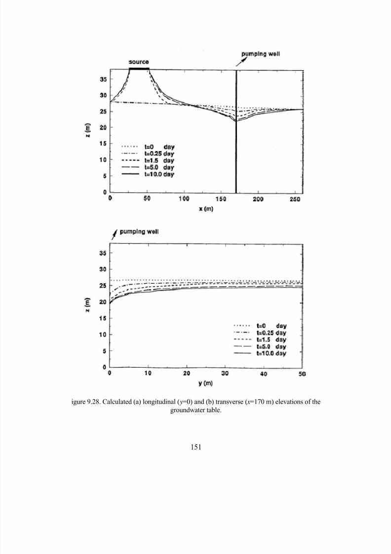
8/20/2019 HYDRUS3D Technical Manual.pdf
http://slidepdf.com/reader/full/hydrus3d-technical-manualpdf 181/260
151
igure 9.28. Calculated (a) longitudinal ( y=0) and (b) transverse ( x=170 m) elevations of thegroundwater table.

8/20/2019 HYDRUS3D Technical Manual.pdf
http://slidepdf.com/reader/full/hydrus3d-technical-manualpdf 182/260
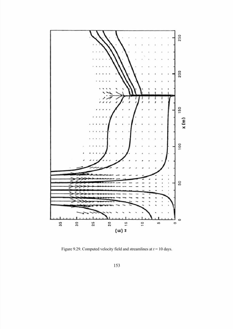
8/20/2019 HYDRUS3D Technical Manual.pdf
http://slidepdf.com/reader/full/hydrus3d-technical-manualpdf 183/260
153
Figure 9.29. Computed velocity field and streamlines at t = 10 days.
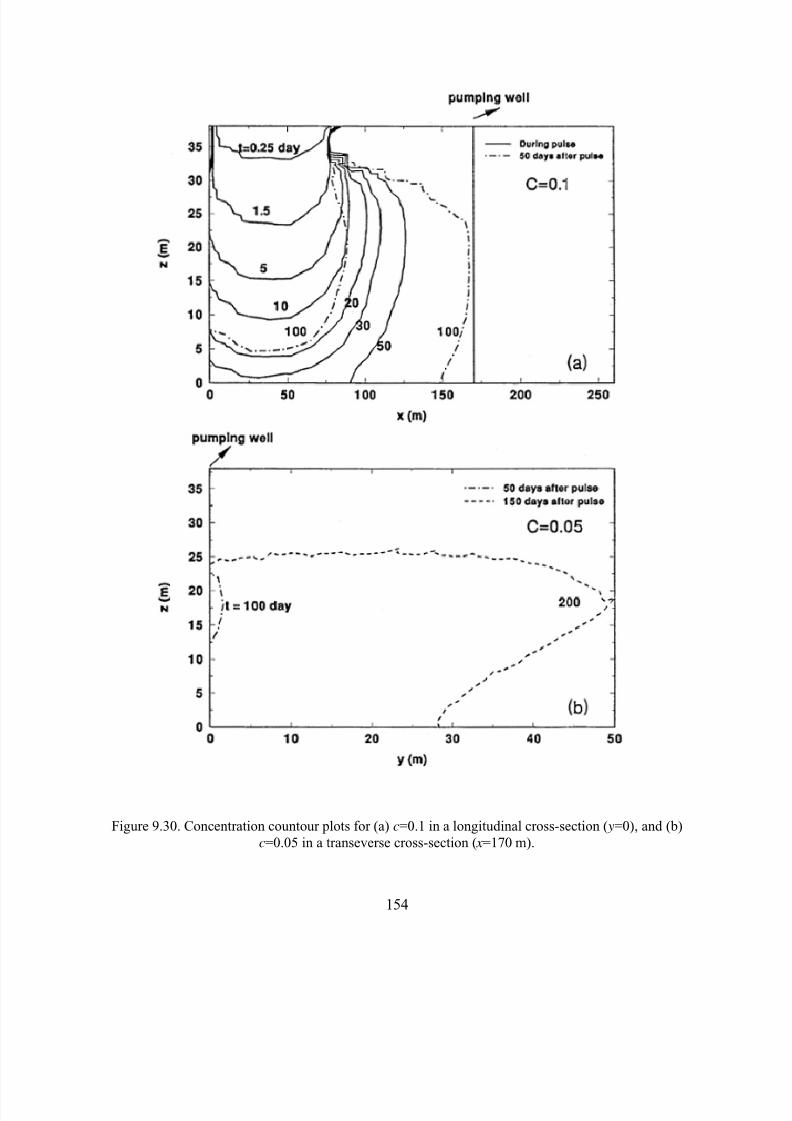
8/20/2019 HYDRUS3D Technical Manual.pdf
http://slidepdf.com/reader/full/hydrus3d-technical-manualpdf 184/260
154
Figure 9.30. Concentration countour plots for (a) c=0.1 in a longitudinal cross-section ( y=0), and (b)c=0.05 in a transeverse cross-section ( x=170 m).
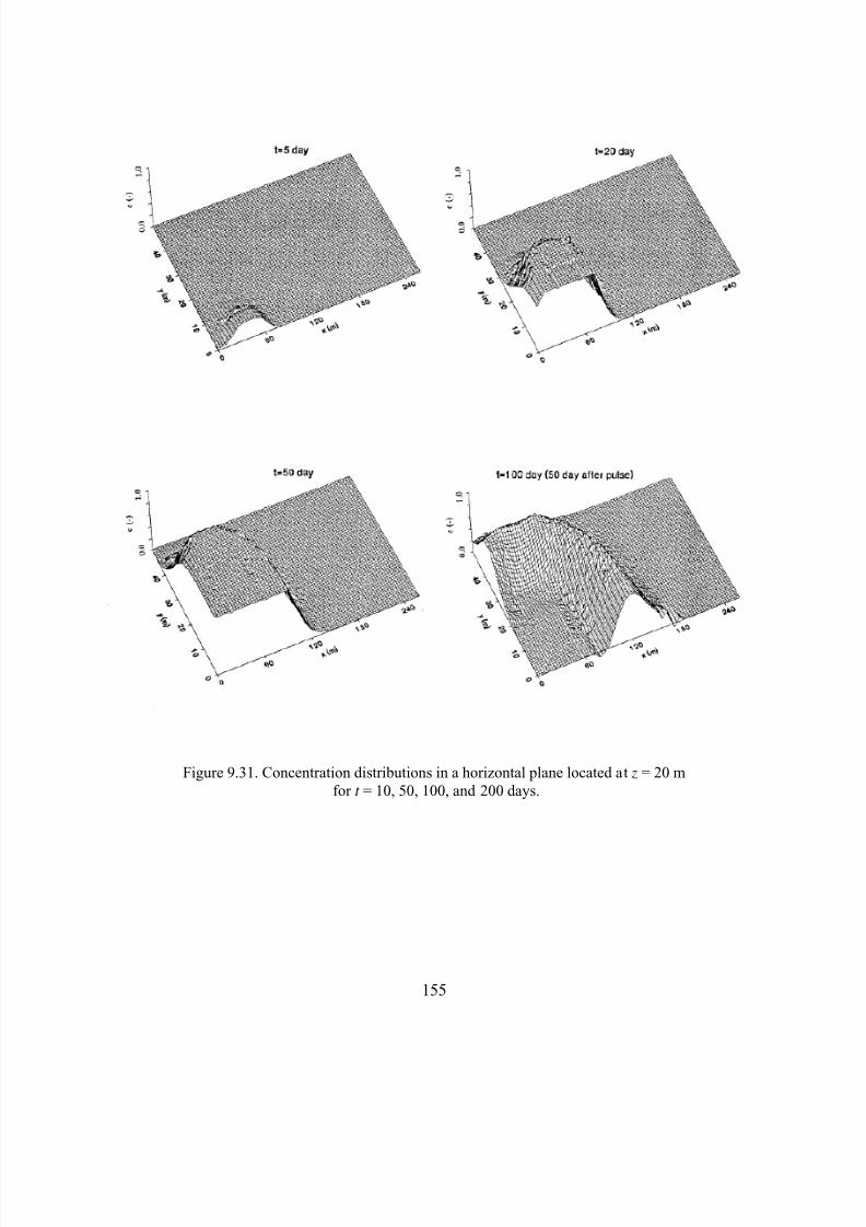
8/20/2019 HYDRUS3D Technical Manual.pdf
http://slidepdf.com/reader/full/hydrus3d-technical-manualpdf 185/260
155
Figure 9.31. Concentration distributions in a horizontal plane located at z = 20 mfor t = 10, 50, 100, and 200 days.
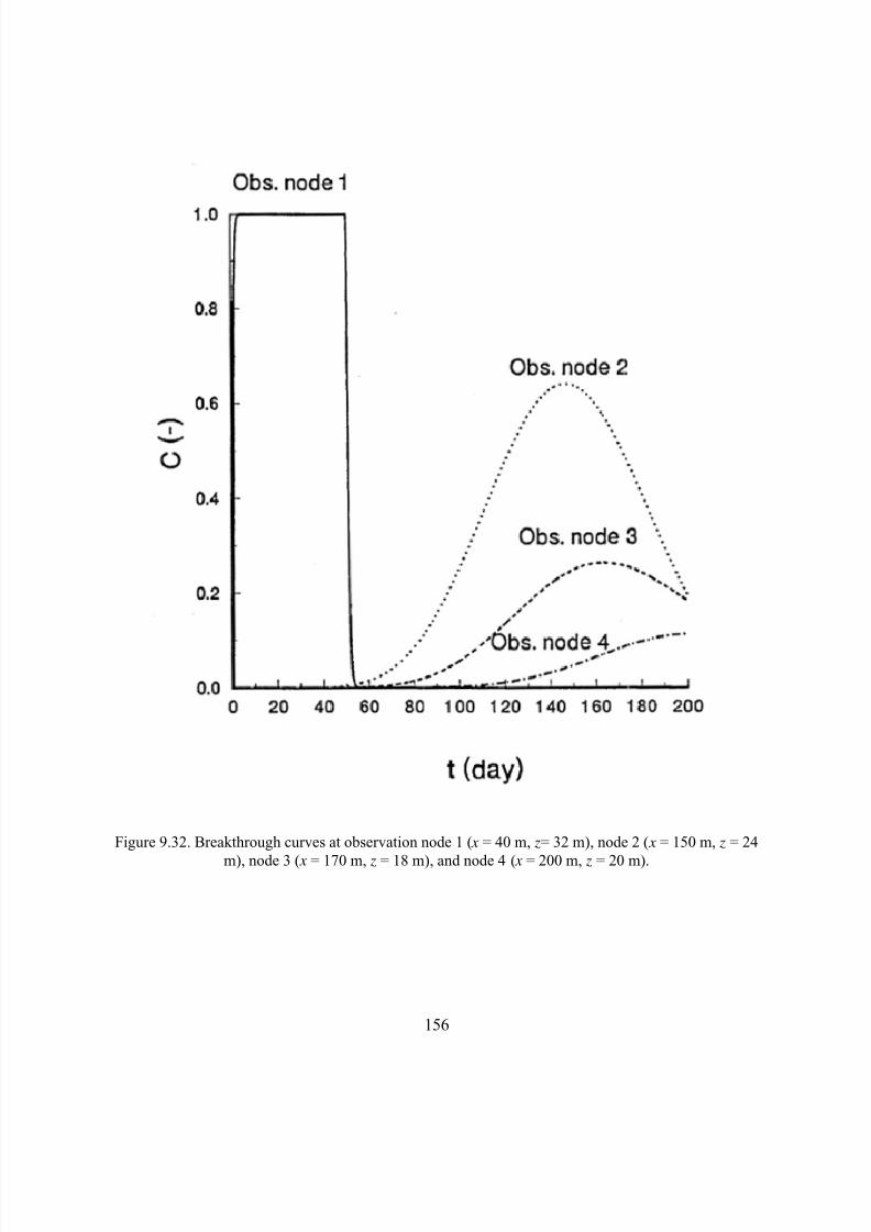
8/20/2019 HYDRUS3D Technical Manual.pdf
http://slidepdf.com/reader/full/hydrus3d-technical-manualpdf 186/260
156
Figure 9.32. Breakthrough curves at observation node 1 ( x = 40 m, z= 32 m), node 2 ( x = 150 m, z = 24
m), node 3 ( x = 170 m, z = 18 m), and node 4 ( x = 200 m, z = 20 m).
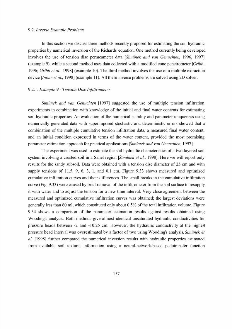
8/20/2019 HYDRUS3D Technical Manual.pdf
http://slidepdf.com/reader/full/hydrus3d-technical-manualpdf 187/260
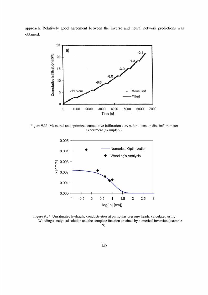
8/20/2019 HYDRUS3D Technical Manual.pdf
http://slidepdf.com/reader/full/hydrus3d-technical-manualpdf 188/260
158
approach. Relatively good agreement between the inverse and neural network predictions was
obtained.
Figure 9.33. Measured and optimized cumulative infiltration curves for a tension disc infiltrometerexperiment (example 9).
0.000
0.001
0.002
0.003
0.004
0.005
-1 -0.5 0 0.5 1 1.5 2 2.5 3
log(|h| [cm])
K
[ c m / s ]
Numerical Optimization
Wooding's Analysis
Figure 9.34. Unsaturated hydraulic conductivities at particular pressure heads, calculated using
Wooding's analytical solution and the complete function obtained by numerical inversion (example9).
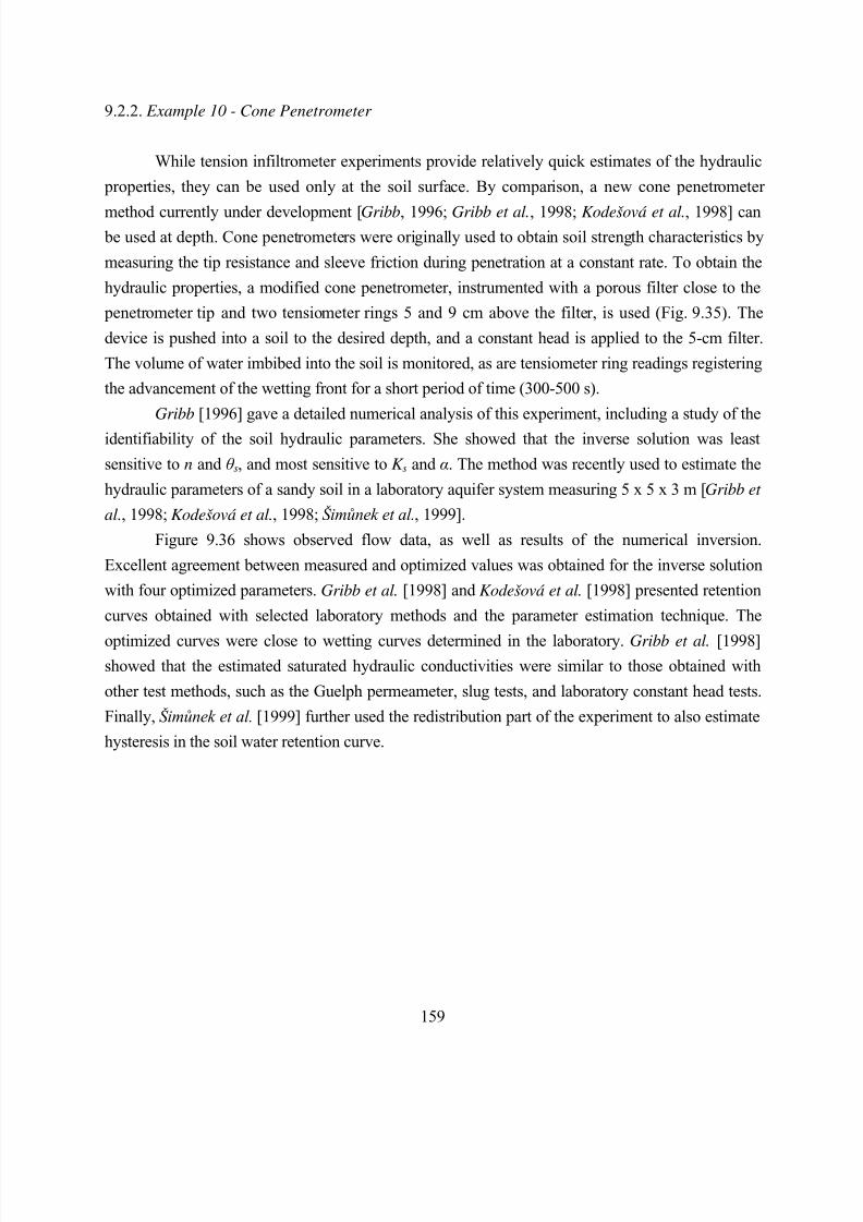
8/20/2019 HYDRUS3D Technical Manual.pdf
http://slidepdf.com/reader/full/hydrus3d-technical-manualpdf 189/260
159
9.2.2. Example 10 - Cone Penetrometer
While tension infiltrometer experiments provide relatively quick estimates of the hydraulic
properties, they can be used only at the soil surface. By comparison, a new cone penetrometer
method currently under development [Gribb, 1996; Gribb et al., 1998; Kodešová et al., 1998] can be used at depth. Cone penetrometers were originally used to obtain soil strength characteristics by
measuring the tip resistance and sleeve friction during penetration at a constant rate. To obtain the
hydraulic properties, a modified cone penetrometer, instrumented with a porous filter close to the
penetrometer tip and two tensiometer rings 5 and 9 cm above the filter, is used (Fig. 9.35). The
device is pushed into a soil to the desired depth, and a constant head is applied to the 5-cm filter.
The volume of water imbibed into the soil is monitored, as are tensiometer ring readings registering
the advancement of the wetting front for a short period of time (300-500 s).
Gribb [1996] gave a detailed numerical analysis of this experiment, including a study of the
identifiability of the soil hydraulic parameters. She showed that the inverse solution was least
sensitive to n and θ s, and most sensitive to K s and α. The method was recently used to estimate the
hydraulic parameters of a sandy soil in a laboratory aquifer system measuring 5 x 5 x 3 m [Gribb et
al., 1998; Kodešová et al., 1998; Šimůnek et al., 1999].
Figure 9.36 shows observed flow data, as well as results of the numerical inversion.
Excellent agreement between measured and optimized values was obtained for the inverse solution
with four optimized parameters. Gribb et al. [1998] and Kodešová et al. [1998] presented retention
curves obtained with selected laboratory methods and the parameter estimation technique. The
optimized curves were close to wetting curves determined in the laboratory. Gribb et al. [1998]showed that the estimated saturated hydraulic conductivities were similar to those obtained with
other test methods, such as the Guelph permeameter, slug tests, and laboratory constant head tests.
Finally, Šimůnek et al. [1999] further used the redistribution part of the experiment to also estimate
hysteresis in the soil water retention curve.
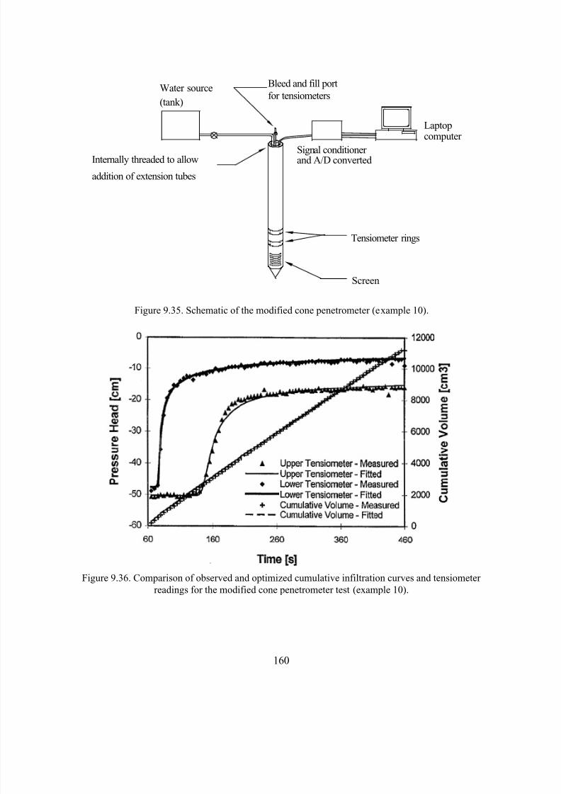
8/20/2019 HYDRUS3D Technical Manual.pdf
http://slidepdf.com/reader/full/hydrus3d-technical-manualpdf 190/260
160
Bleed and fill portfor tensiometers
Signal conditioner and A/D converted
Laptop
computer
Water source
(tank)
Internally threaded to allow
addition of extension tubes
Tensiometer rings
Screen
Figure 9.35. Schematic of the modified cone penetrometer (example 10).
Figure 9.36. Comparison of observed and optimized cumulative infiltration curves and tensiometerreadings for the modified cone penetrometer test (example 10).
8/20/2019 HYDRUS3D Technical Manual.pdf
http://slidepdf.com/reader/full/hydrus3d-technical-manualpdf 191/260
161
9.2.3. Example 11 - Multiple-Step Extraction Experiment
The tension infiltrometer and cone penetrometer methods provide information about the
wetting branches of the soil hydraulic properties. By comparison, a multiple step extraction device
can be used to obtain draining branches. The device consists of a ceramic soil solution sampler(Fig. 9.37), which is inserted into an initially wet soil profile and subjected to a series of vacuum
extraction pressures. The cumulative amount of soil solution extracted during an experiment, as
well as pressure heads at various locations near the extraction device, are monitored during the
experiment and subsequently used in an objective function for the nonlinear minimization problem.
Inoue et al. [1998] first evaluated the feasibility of the vacuum extraction technique using
numerically generated data, and concluded that the method is well suited for loamy-textured soils,
but not necessarily for sandy soils. They tested the method in the laboratory and in the field. Here
we briefly discuss one laboratory application.
The experiment [ Inoue et al., 1998] was carried out on a Columbia fine sandy loam. The
center of the ceramic ring (with a radius of 3 cm, and a length of 3 cm) was located 6.3 cm below
the soil surface. The tensiometers were installed at the following positions: T1(r,z)=(4,-6.3 cm),
T2=(6,-6.3), T3=(6,-24). Five vacuum extraction steps were applied: hex=-35 cm for 25 h, hex=-65
cm for 25 < t < 73 h, hex=-125 cm for 73 < t < 217 h, hex=-240 cm for 217 < t < 339 h, and finally
hex=-480 cm for 339 < t < 605 h. Experimental data, as well as the final results of the numerical
inversion, are presented in Figure 9.38. The saturated hydraulic conductivity of the ceramic ring
was optimized simultaneously with van Genuchten's hydraulic parameters. Agreement between
measured and calculated values in Figure 9.38 was relatively good. Inoue et al. [1998] comparedthe optimized soil hydraulic functions with independently measured data.

8/20/2019 HYDRUS3D Technical Manual.pdf
http://slidepdf.com/reader/full/hydrus3d-technical-manualpdf 192/260
162
Figure 9.37. Layout of laboratory multistep extraction experiment (example 11).
Figure 9.38. Comparison of measured (symbols) and optimized (lines) cumulative extraction (a) and pressure head (b) values (example 11).
8/20/2019 HYDRUS3D Technical Manual.pdf
http://slidepdf.com/reader/full/hydrus3d-technical-manualpdf 193/260
163
10. INPUT DATA
The input data for HYDRUS are given in seven separate input files. These input files
consist of one or more input blocks identified by the letters from A through M. The input files and
blocks must be arranged as follows:
SELECTOR.INA. Basic InformationB. Material InformationC. Time InformationD. Solute Transport InformationE. Heat Transport InformationF. Root Water Uptake Information
MESHTRIA.TXTG. Finite Element Mesh Information
DOMAIN.DATH. Nodal InformationI. Element Information
BOUNDARY.INJ. Boundary Information
ATMOSPH.INK. Atmospheric Information
DIMENSIO.INL. Dimension Information
FIT.INM. Inverse Solution Information
CROSSSECT.IN N. Mesh Lines Information
The various input blocks are described in detail below. Tables 10.1 through 10.14 describe
the data required for each input block. All data are read in using list-directed formatting (free
format). Comment lines are provided at the beginning of, and within, each input block to facilitate,among other things, proper identification of the function of the block and the input variables. The
comment lines are ignored during program execution; hence, they may be left blank but should not
be omitted. All input files must be placed into one subdirectory. Output files are printed into the
8/20/2019 HYDRUS3D Technical Manual.pdf
http://slidepdf.com/reader/full/hydrus3d-technical-manualpdf 194/260
164
same subdirectory. An additional file Level_01.dir, which specifies the path to the input and output
file subdirectory must be given in the same directory as the executable HYDRUS codes if
numerical solvers are to be run outside of the GUI. The program assumes that all input data are
specified in a consistent set of units for mass M, length L, and time T. The values of temperature
should be specified in degrees Celsius.Most of the information in Tables 10.1 through 10.14 should be self-explanatory. Several
input files can be alternatively entered using binary files, e.g. the DOMAIN.DAT file can be
replaced with the binary DOMAIN.IN file, and the MESHTRIA.TXT file can be replaced with the
MESHTRIA.000 (or MESHGEN2.PMG) binary file. Binary files are utilized by default when the
HYDRUS user interface is used.
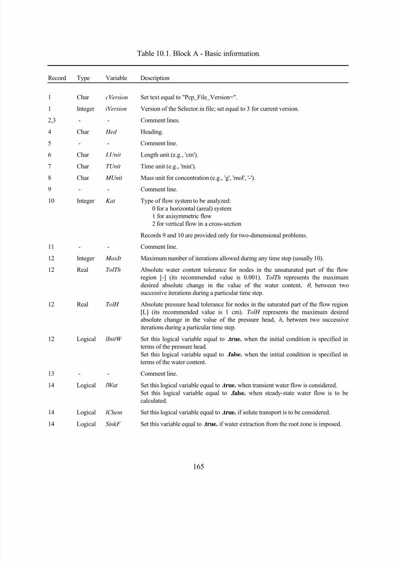
8/20/2019 HYDRUS3D Technical Manual.pdf
http://slidepdf.com/reader/full/hydrus3d-technical-manualpdf 195/260
165
Table 10.1. Block A - Basic information.
Record Type Variable Description
1 Char cVersion Set text equal to "Pcp_File_Version=".1 Integer iVersion Version of the Selector.in file; set equal to 3 for current version.
2,3 - - Comment lines.
4 Char Hed Heading.
5 - - Comment line.
6 Char LUnit Length unit (e.g., 'cm').
7 Char TUnit Time unit (e.g., 'min').
8 Char MUnit Mass unit for concentration (e.g., 'g', 'mol', '-').
9 - - Comment line.
10 Integer Kat Type of flow system to be analyzed:0 for a horizontal (areal) system1 for axisymmetric flow2 for vertical flow in a cross-section
Records 9 and 10 are provided only for two-dimensional problems.
11 - - Comment line.
12 Integer MaxIt Maximum number of iterations allowed during any time step (usually 10).
12 Real TolTh Absolute water content tolerance for nodes in the unsaturated part of the flowregion [-] (its recommended value is 0.001). TolTh represents the maximumdesired absolute change in the value of the water content, θ , between two
successive iterations during a particular time step.12 Real TolH Absolute pressure head tolerance for nodes in the saturated part of the flow region
[L] (its recommended value is 1 cm). TolH represents the maximum desiredabsolute change in the value of the pressure head, h, between two successiveiterations during a particular time step.
12 Logical lInitW Set this logical variable equal to .true. when the initial condition is specified interms of the pressure head.Set this logical variable equal to .false. when the initial condition is specified interms of the water content.
13 - - Comment line.
14 Logical lWat Set this logical variable equal to .true. when transient water flow is considered.
Set this logical variable equal to .false. when steady-state water flow is to becalculated.
14 Logical lChem Set this logical variable equal to .true. if solute transport is to be considered.
14 Logical SinkF Set this variable equal to .true. if water extraction from the root zone is imposed.
8/20/2019 HYDRUS3D Technical Manual.pdf
http://slidepdf.com/reader/full/hydrus3d-technical-manualpdf 196/260
166
Table 10.1. (continued)
Record Type Variable Description
14 Logical ShortF .true. if information is to be printed only at preselected times, but not at eachtime step (T-level information, see Section 11.1),.false. if information is to be printed at each time step or at each n-time steps.
14 Logical lPrintD Set this logical variable equal to .true. if information about the pressure heads,water contents, temperatures, and concentrations in observation nodes, and thewater and solute fluxes is to be printed at a constant time interval tPrintInterval.
14 Logical lScreen Set this logical variable equal to .true. if information is to be printed on the screenduring code execution.
14 Logical AtmInf .true. if atmospheric boundary conditions are supplied via the input fileATMOSPH.IN,.false. if the file ATMOSPH.IN is not provided (i.e., in case of time independent
boundary conditions).14 Logical lTemp Set this logical variable equal to .true. if heat transport is to be considered.
14 Logical lWDep .true. if hydraulic properties are to be considered as temperature dependent..false. otherwise (see Section 2.5).
14 Logical lEquil .true. if equilibrium solute transport is considered..false. if nonequilibrium solute transport is considered for at least one solutespecies.
14 Logical lExter Set this logical variable equal to .true. if an external mesh generator is to be used togenerate the finite element mesh (i.e., when using MESHGEN-2D).Set this logical variable equal to .false. if an internal mesh generator for simplequadrilateral domains is to be used to generate the finite element mesh.
14 Logical lInv Set this logical variable equal to .true. if the soil hydraulic or solute transport parameters are to be estimated from measured data (available only for 2Dapplications).Set this logical variable equal to .false. if only the direct solution for a particular
problem is to be carried out.
15 - - Comment line.
16 Logical lUnsatch Set this logical variable equal to .true. if the major ion chemistry module(Unsatchem) is to be used to simulate solute transport.
16 Logical lActRSU Set this logical variable equal to .true. if the Active Solute Transport model is to be used [Šimůnek and Hopmans, 2009].
16 Logical lDummy Logical dummy variable (repeat 7 times).17 - - Comment line.
17 Integer nPrintSteps Information to the screen and output files is not printed at each time step, butafter each nPrintSteps.
8/20/2019 HYDRUS3D Technical Manual.pdf
http://slidepdf.com/reader/full/hydrus3d-technical-manualpdf 197/260
167
Table 10.1. (continued)
Record Type Variable Description
17 Real tPrintInterval A constant time interval after which information about the pressure heads,water contents, temperatures, and concentrations in observation nodes, and thewater and solute fluxes is to be printed.
17 Logical lEnter Set this logical variable equal to .true. if the Enter key is to be pressed at theend of simulation.
8/20/2019 HYDRUS3D Technical Manual.pdf
http://slidepdf.com/reader/full/hydrus3d-technical-manualpdf 198/260
168
Table 10.2. Block B - Material information.
Record Type Variable Description
1,2 - - Comment lines.3 Integer NMat Number of soil materials. Materials are identified by the material number,
MatNum, specified in Block H.
3 Integer NLay Number of subregions for which separate water balances are being computed.Subregions are identified by the subregion number, LayNum, specified in Block I.
3 Real ha Absolute value of the upper limit [L] of the pressure head interval below which atable of hydraulic properties will be generated internally for each material (ha must be greater than 0.0; e.g. 0.001 cm) (see Section 5.3.11).
3 Real hb Absolute value of the lower limit [L] of the pressure head interval for which a tableof hydraulic properties will be generated internally for each material (e.g. 1000 m).One may assign to hb the highest (absolute) expected pressure head to be expected
during a simulation. If the absolute value of the pressure head during programexecution lies outside of the interval [ha ,hb], then appropriate values for thehydraulic properties are computed directly from the hydraulic functions (i.e.,without interpolation in the table). Zero values for both ha and hb should bespecified when interpolation tables are not to be used.
3 Integer NAniz Number of anisotropy tensors used in the transport domain (minimum number is1). This value needs to be provided only for three-dimensional applications.
4 - - Comment line.
5 Integer iModel Soil hydraulic properties model:= 0; van Genuchten's [1980] model with six parameters.= 1; modified van Genuchten's model with ten parameters, Vogel and Císlerová [1988].= 2; Brooks and Corey's [1964] model with six parameters.= 3; van Genuchten's [1980] model with air-entry value of -2 cm and with six parameters.= 4; Kosugi’s [1996] model with six parameters.= 5; dual porosity model of Durner [1994] with nine parameters.= 6; dual-porosity system with transfer proportional to the effective saturation (9 parameters) (see Sections 2.1.2 and 2.8).= 7; dual-porosity system with transfer proportional to the pressure head (11 parameters) (see Sections 2.1.2 and 2.8).
5 Integer iHyst Hysteresis in the soil hydraulic properties:= 0; No hysteresis= 1; Hysteresis in the retention curve only
= 2; Hysteresis in both the retention and hydraulic conductivity functions= 3; Hysteresis using Bob Lenhard’s model [ Lenhard et al., 1991; Lenhard andParker , 1992].
6 - - Comment line.
8/20/2019 HYDRUS3D Technical Manual.pdf
http://slidepdf.com/reader/full/hydrus3d-technical-manualpdf 199/260
169
Table 10.2. (continued)
Record Type Variable Description
7 Integer iKappa = -1 if the initial condition is to be calculated from the main drying branch.= 1 if the initial condition is to be calculated from the main wetting branch.
Records 6 and 7 are provided only when iHyst > 0.
8 - - Comment line.
9 Real Par (1, M ) Parameter θ r for material M [-].9 Real Par (2, M ) Parameter θ s for material M [-].9 Real Par (3, M ) Parameter α for material M [L-1].9 Real Par (4, M ) Parameter n for material M [-].9 Real Par (5, M ) Parameter K s for material M [LT-1].9 Real Par (6, M ) Parameter l for material M [-].
The following four parameters are specified only when iModel=1.9 Real Par (7, M ) Parameter θ m for material M [-].9 Real Par (8, M ) Parameter θ a for material M [-].9 Real Par (9, M ) Parameter θ k for material M [-].9 Real Par (10, M ) Parameter K k for material M [LT-1].
The following four parameters are specified only when iModel=0 and iHyst >1.9 Real Par (7, M ) Parameter θ m for material M [-].9 Real Par (8, M ) Parameter θ s
w for material M [-].9 Real Par (9, M ) Parameter α w for material M [L-1].9 Real Par (10, M ) Parameter K s
w for material M [LT-1].
The following three parameters are specified only when iModel=5 [ Durner ,
1994].9 Real Par (7, M ) Parameter w for material M [-]. The weighting factor for the sub-curve for thesecond overlapping subregion.
9 Real Par (8, M ) Parameter α for material M [L-1] for the second overlapping subregion.9 Real Par (9, M ) Parameter n for material M [-] for the second overlapping subregion.
The following four parameters are specified only when iModel=6 (dual-porositysystem with transfer proportional to the water content gradient).
9 Real Par (7, M ) Parameter θ r im for the immobile region of material M [-].
9 Real Par (8, M ) Parameter θ sim for the immobile region of material M [-].
9 Real Par (9, M ) Parameter ω (mass transfer coefficient in (2.63)) for material M [-].
The following four parameters are specified only when iModel=7 (dual-porositysystem with transfer proportional to the pressure head gradient).
9 Real Par (7, M ) Parameter θ r im for the immobile region of material M [-].9 Real Par (8, M ) Parameter θ s
im for the immobile region of material M [-].9 Real Par (9, M ) Parameter α
im for the immobile region of material M [-].9 Real Par (10, M ) Parameter nim for the immobile region of material M [-].9 Real Par (11, M ) Parameter K a (mass transfer coefficient in (2.67)) for material M [-].
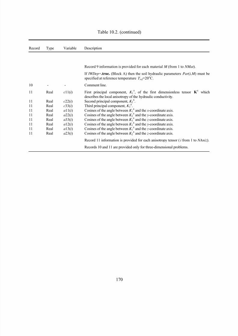
8/20/2019 HYDRUS3D Technical Manual.pdf
http://slidepdf.com/reader/full/hydrus3d-technical-manualpdf 200/260
170
Table 10.2. (continued)
Record Type Variable Description
Record 9 information is provided for each material M (from 1 to NMat ).
If lWDep=.true. (Block A) then the soil hydraulic parameters Par (i,M ) must bespecified at reference temperature T ref =20oC.
10 - - Comment line.
11 Real c11(i) First principal component, K 1 A, of the first dimensionless tensor K
A whichdescribes the local anisotropy of the hydraulic conductivity.
11 Real c22(i) Second principal component, K 2 A.
11 Real c33(i) Third principal component, K 3 A.
11 Real a11(i) Cosines of the angle between K 1 A and the x-coordinate axis.
11 Real a22(i) Cosines of the angle between K 2 A and the y-coordinate axis.
11 Real a33(i) Cosines of the angle between K 3 A and the z-coordinate axis.11 Real a12(i) Cosines of the angle between K 1
A and the y-coordinate axis.11 Real a13(i) Cosines of the angle between K 1
A and the z-coordinate axis.11 Real a23(i) Cosines of the angle between K 2
A and the z-coordinate axis.
Record 11 information is provided for each anisotropy tensor (i from 1 to NAniz).
Records 10 and 11 are provided only for three-dimensional problems.
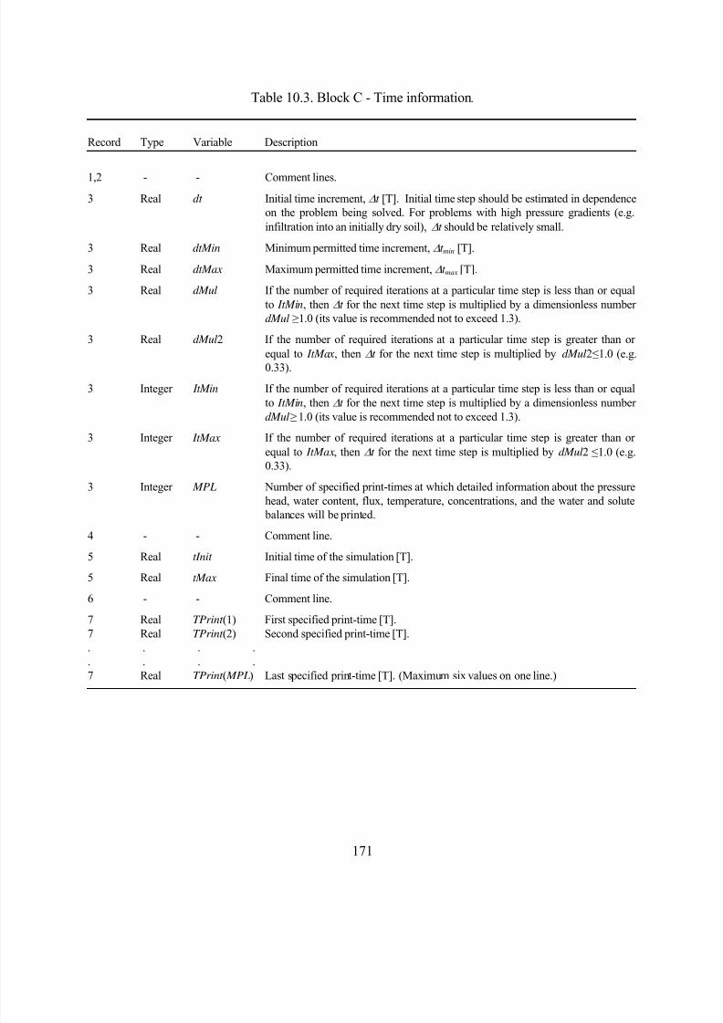
8/20/2019 HYDRUS3D Technical Manual.pdf
http://slidepdf.com/reader/full/hydrus3d-technical-manualpdf 201/260
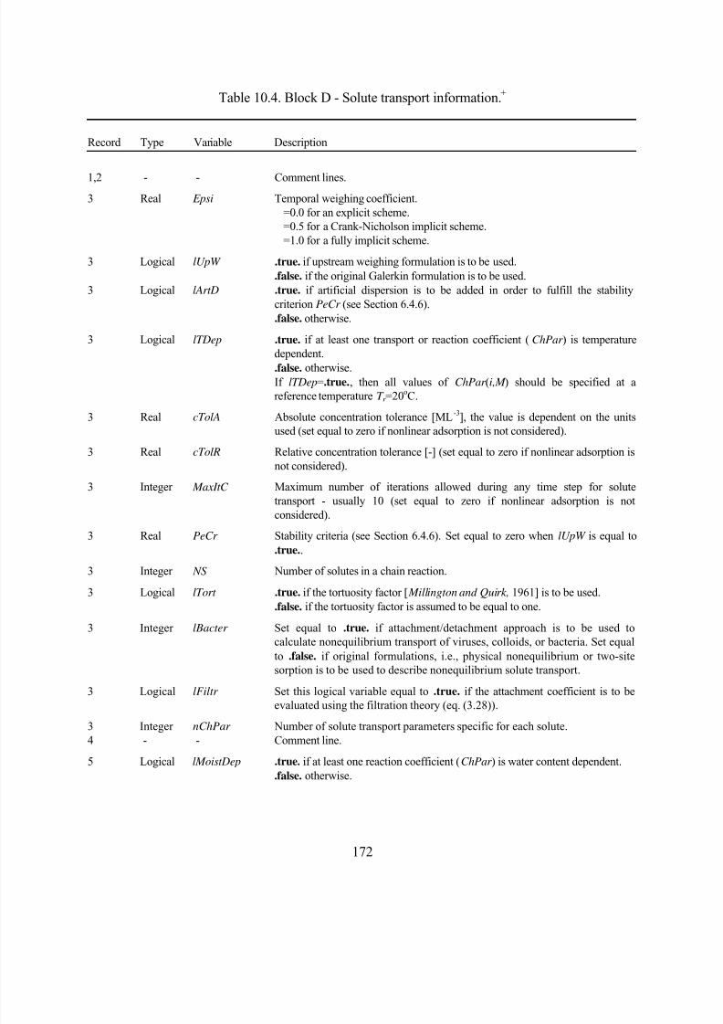
8/20/2019 HYDRUS3D Technical Manual.pdf
http://slidepdf.com/reader/full/hydrus3d-technical-manualpdf 202/260
172
Table 10.4. Block D - Solute transport information.+
Record Type Variable Description
1,2 - - Comment lines.3 Real Epsi Temporal weighing coefficient.
=0.0 for an explicit scheme.=0.5 for a Crank-Nicholson implicit scheme.=1.0 for a fully implicit scheme.
3 Logical lUpW .true. if upstream weighing formulation is to be used..false. if the original Galerkin formulation is to be used.
3 Logical lArtD .true. if artificial dispersion is to be added in order to fulfill the stabilitycriterion PeCr (see Section 6.4.6)..false. otherwise.
3 Logical lTDep .true. if at least one transport or reaction coefficient (ChPar ) is temperature
dependent..false. otherwise.If lTDep=.true., then all values of ChPar (i,M ) should be specified at areference temperature T r =20oC.
3 Real cTolA Absolute concentration tolerance [ML-3], the value is dependent on the unitsused (set equal to zero if nonlinear adsorption is not considered).
3 Real cTolR Relative concentration tolerance [-] (set equal to zero if nonlinear adsorption isnot considered).
3 Integer MaxItC Maximum number of iterations allowed during any time step for solutetransport - usually 10 (set equal to zero if nonlinear adsorption is notconsidered).
3 Real PeCr Stability criteria (see Section 6.4.6). Set equal to zero when lUpW is equal to.true..
3 Integer NS Number of solutes in a chain reaction.
3 Logical lTort .true. if the tortuosity factor [ Millington and Quirk, 1961] is to be used..false. if the tortuosity factor is assumed to be equal to one.
3 Integer lBacter Set equal to .true. if attachment/detachment approach is to be used tocalculate nonequilibrium transport of viruses, colloids, or bacteria. Set equalto .false. if original formulations, i.e., physical nonequilibrium or two-sitesorption is to be used to describe nonequilibrium solute transport.
3 Logical lFiltr Set this logical variable equal to .true. if the attachment coefficient is to beevaluated using the filtration theory (eq. (3.28)).
3 Integer nChPar Number of solute transport parameters specific for each solute.4 - - Comment line.
5 Logical lMoistDep .true. if at least one reaction coefficient (ChPar ) is water content dependent..false. otherwise.
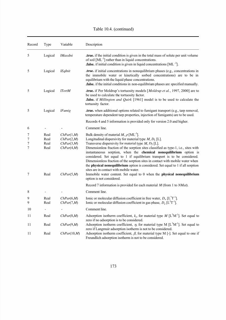
8/20/2019 HYDRUS3D Technical Manual.pdf
http://slidepdf.com/reader/full/hydrus3d-technical-manualpdf 203/260
173
Table 10.4. (continued)
Record Type Variable Description
5 Logical lMassIni .true. if the initial condition is given in the total mass of solute per unit volumeof soil [ML-3] rather than in liquid concentrations..false. if initial condition is given in liquid concentrations [ML-3].
5 Logical lEqInit .true. if initial concentrations in nonequilibrium phases (e.g., concentrations inthe immobile water or kinetically sorbed concentrations) are to be inequilibrium with the liquid phase concentrations..false. if the initial conditions in non-equilibrium phases are specified manually.
5 Logical lTortM .true. if Per Moldrup’s tortuosity models [ Moldrup et al., 1997, 2000] are to be used to calculate the tortuosity factor..false. if Millington and Quirk [1961] model is to be used to calculate thetortuosity factor.
5 Logical lFumig .true. when additional options related to fumigant transport (e.g., tarp removal,temperature dependent tarp properties, injection of fumigants) are to be used.
Records 4 and 5 information is provided only for version 2.0 and higher.
6 - - Comment line.
7 Real ChPar (1, M ) Bulk density of material M , ρ [ML-3].7 Real ChPar (2, M ) Longitudinal dispersivity for material type M , D L [L].7 Real ChPar (3, M ) Transverse dispersivity for material type M , DT [L].7 Real ChPar (4, M ) Dimensionless fraction of the sorption sites classified as type-1, i.e., sites with
instantaneous sorption, when the chemical nonequilibrium option isconsidered. Set equal to 1 if equilibrium transport is to be considered.Dimensionless fraction of the sorption sites in contact with mobile water whenthe physical nonequilibrium option is considered. Set equal to 1 if all sorptionsites are in contact with mobile water.
7 Real ChPar (5, M ) Immobile water content. Set equal to 0 when the physical nonequilibrium option is not considered.
Record 7 information is provided for each material M (from 1 to NMat ).
8 - - Comment line.
9 Real ChPar (6, M ) Ionic or molecular diffusion coefficient in free water, Dw [L2T-1].9 Real ChPar (7, M ) Ionic or molecular diffusion coefficient in gas phase, Dg [L
2T-1].
10 - - Comment line.
11 Real ChPar (8, M ) Adsorption isotherm coefficient, k s, for material type M [L3M-1]. Set equal tozero if no adsorption is to be considered.
11 Real ChPar (9, M ) Adsorption isotherm coefficient, η , for material type M [L3M-1]. Set equal tozero if Langmuir adsorption isotherm is not to be considered.
11 Real ChPar (10, M ) Adsorption isotherm coefficient, β , for material type M [-]. Set equal to one ifFreundlich adsorption isotherm is not to be considered.
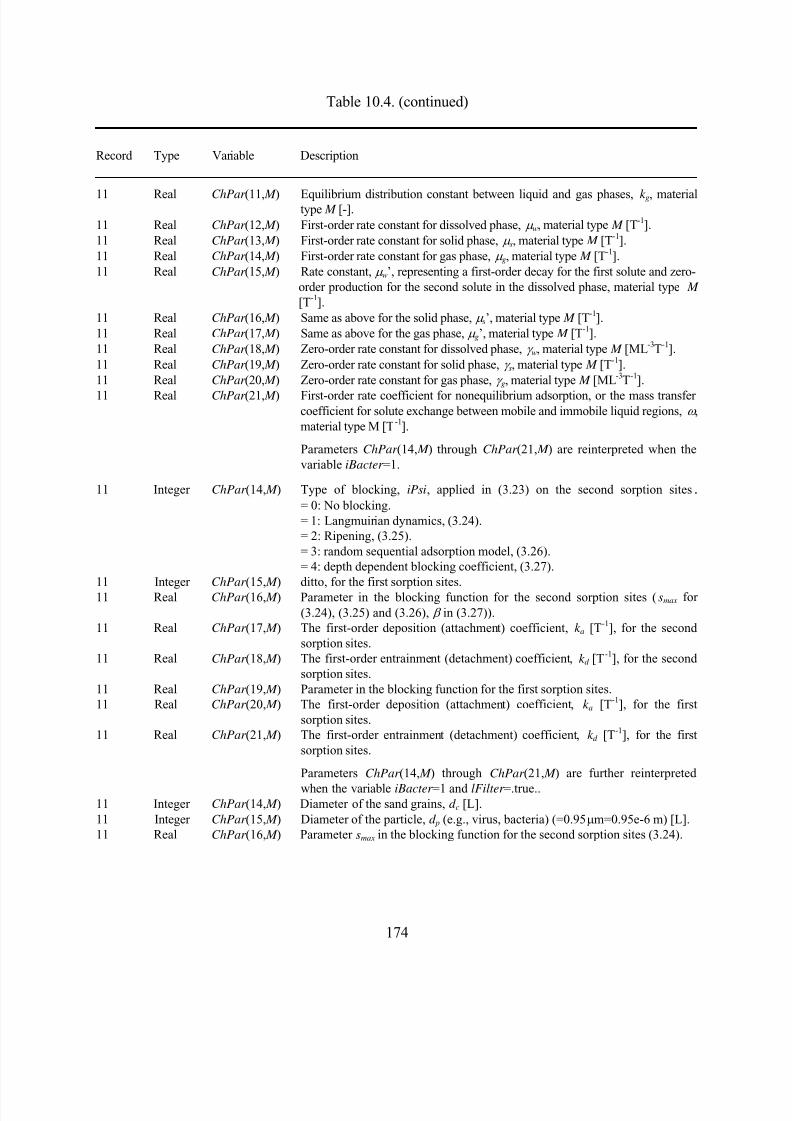
8/20/2019 HYDRUS3D Technical Manual.pdf
http://slidepdf.com/reader/full/hydrus3d-technical-manualpdf 204/260
174
Table 10.4. (continued)
Record Type Variable Description
11 Real ChPar (11, M ) Equilibrium distribution constant between liquid and gas phases, k g, materialtype M [-].11 Real ChPar (12, M ) First-order rate constant for dissolved phase, µ w, material type M [T-1].11 Real ChPar (13, M ) First-order rate constant for solid phase, µ s, material type M [T-1].11 Real ChPar (14, M ) First-order rate constant for gas phase, µ g, material type M [T-1].11 Real ChPar (15, M ) Rate constant, µ w’, representing a first-order decay for the first solute and zero-
order production for the second solute in the dissolved phase, material type M [T-1].
11 Real ChPar (16, M ) Same as above for the solid phase, µ s’, material type M [T-1].11 Real ChPar (17, M ) Same as above for the gas phase, µ g’, material type M [T-1].11 Real ChPar (18, M ) Zero-order rate constant for dissolved phase, γ w, material type M [ML-3T-1].11 Real ChPar (19, M ) Zero-order rate constant for solid phase, γ s, material type M [T-1].11 Real ChPar (20, M ) Zero-order rate constant for gas phase, γ g, material type M [ML-3T-1].
11 Real ChPar (21, M ) First-order rate coefficient for nonequilibrium adsorption, or the mass transfercoefficient for solute exchange between mobile and immobile liquid regions, ω ,material type M [T-1].
Parameters ChPar (14, M ) through ChPar (21, M ) are reinterpreted when thevariable iBacter =1.
11 Integer ChPar (14, M ) Type of blocking, iPsi, applied in (3.23) on the second sorption sites.= 0: No blocking.= 1: Langmuirian dynamics, (3.24).= 2: Ripening, (3.25).= 3: random sequential adsorption model, (3.26).= 4: depth dependent blocking coefficient, (3.27).
11 Integer ChPar (15, M ) ditto, for the first sorption sites.11 Real ChPar (16, M ) Parameter in the blocking function for the second sorption sites (smax for
(3.24), (3.25) and (3.26), β in (3.27)).11 Real ChPar (17, M ) The first-order deposition (attachment) coefficient, k a [T-1], for the second
sorption sites.11 Real ChPar (18, M ) The first-order entrainment (detachment) coefficient, k d [T
-1], for the secondsorption sites.
11 Real ChPar (19, M ) Parameter in the blocking function for the first sorption sites.11 Real ChPar (20, M ) The first-order deposition (attachment) coefficient, k a [T-1], for the first
sorption sites.11 Real ChPar (21, M ) The first-order entrainment (detachment) coefficient, k d [T-1], for the first
sorption sites.
Parameters ChPar (14, M ) through ChPar (21, M ) are further reinterpreted
when the variable iBacter =1 and lFilter =.true..11 Integer ChPar (14, M ) Diameter of the sand grains, d c [L].11 Integer ChPar (15, M ) Diameter of the particle, d p (e.g., virus, bacteria) (=0.95µm=0.95e-6 m) [L].11 Real ChPar (16, M ) Parameter smax in the blocking function for the second sorption sites (3.24).
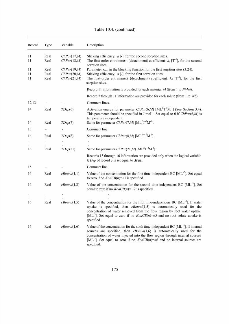
8/20/2019 HYDRUS3D Technical Manual.pdf
http://slidepdf.com/reader/full/hydrus3d-technical-manualpdf 205/260
175
Table 10.4. (continued)
Record Type Variable Description
11 Real ChPar (17, M ) Sticking efficiency, α [-], for the second sorption sites.11 Real ChPar (18, M ) The first-order entrainment (detachment) coefficient, k d [T-1], for the second
sorption sites.11 Real ChPar (19, M ) Parameter smax in the blocking function for the first sorption sites (3.24).11 Real ChPar (20, M ) Sticking efficiency, α [-], for the first sorption sites.11 Real ChPar (21, M ) The first-order entrainment (detachment) coefficient, k d [T-1], for the first
sorption sites.
Record 11 information is provided for each material M (from 1 to NMat ).
Record 7 through 11 information are provided for each solute (from 1 to NS ).
12,13 - - Comment lines.
14 Real TDep(6) Activation energy for parameter ChPar (6, M ) [ML2T-2M-1] (See Section 3.4).
This parameter should be specified in J mol-1. Set equal to 0 if ChPar (6, M ) istemperature independent.
14 Real TDep(7) Same for parameter ChPar (7, M ) [ML2T-2M-1].
15 - - Comment line.
16 Real TDep(8) Same for parameter ChPar (8, M ) [ML2T-2M-1].. . . .. . . .16 Real TDep(21) Same for parameter ChPar (21, M ) [ML2T-2M-1].
Records 13 through 16 information are provided only when the logical variablelTDep of record 3 is set equal to .true..
15 - - Comment line.
16 Real cBound (1,1) Value of the concentration for the first time-independent BC [ML-3]. Set equalto zero if no KodCB(n)=±1 is specified.
16 Real cBound (1,2) Value of the concentration for the second time-independent BC [ML-3]. Setequal to zero if no KodCB(n)= ±2 is specified.
. . . .
. . . .16 Real cBound (1,5) Value of the concentration for the fifth time-independent BC [ML-3]. If water
uptake is specified, then cBound (1,5) is automatically used for theconcentration of water removed from the flow region by root water uptake[ML-3]. Set equal to zero if no KodCB(n)=±5 and no root solute uptake isspecified.
16 Real cBound (1,6) Value of the concentration for the sixth time-independent BC [ML-3
]. If internalsources are specified, then cBound (1,6) is automatically used for theconcentration of water injected into the flow region through internal sources[ML-3]. Set equal to zero if no KodCB(n)=±6 and no internal sources arespecified.
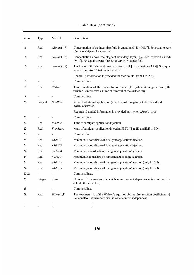
8/20/2019 HYDRUS3D Technical Manual.pdf
http://slidepdf.com/reader/full/hydrus3d-technical-manualpdf 206/260
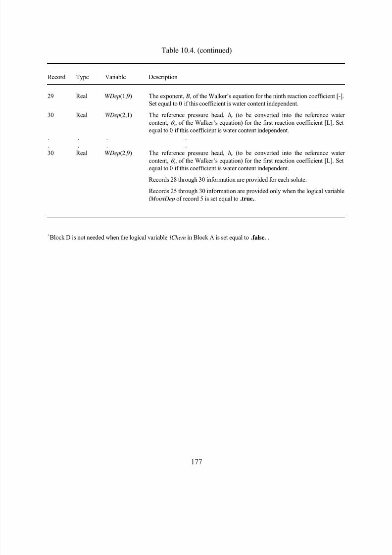
8/20/2019 HYDRUS3D Technical Manual.pdf
http://slidepdf.com/reader/full/hydrus3d-technical-manualpdf 207/260
177
Table 10.4. (continued)
Record Type Variable Description
29 Real WDep(1,9) The exponent, B, of the Walker’s equation for the ninth reaction coefficient [-].Set equal to 0 if this coefficient is water content independent.
30 Real WDep(2,1) The reference pressure head, hr (to be converted into the reference watercontent, θ r , of the Walker’s equation) for the first reaction coefficient [L]. Setequal to 0 if this coefficient is water content independent.
. . . .
. . . .30 Real WDep(2,9) The reference pressure head, hr (to be converted into the reference water
content, θ r , of the Walker’s equation) for the first reaction coefficient [L]. Setequal to 0 if this coefficient is water content independent.
Records 28 through 30 information are provided for each solute.
Records 25 through 30 information are provided only when the logical variablelMoistDep of record 5 is set equal to .true..
+Block D is not needed when the logical variable lChem in Block A is set equal to .false. .
8/20/2019 HYDRUS3D Technical Manual.pdf
http://slidepdf.com/reader/full/hydrus3d-technical-manualpdf 208/260
178
Table 10.5. Block E - Heat transport information.+
Record Type Symbol Description
1,2 - - Comment lines.3 Real TPar (1, M ) Volumetric solid phase fraction of material M , θ n [-].3 Real TPar (2, M ) Volumetric organic matter fraction of material M , θ o [-].3 Real TPar (3, M ) Longitudinal thermal dispersivity of material M , λ L [L].3 Real TPar (4, M ) Transverse thermal dispersivity of material M , λ T [L].3 Real TPar (5, M ) Coefficient b1 in the thermal conductivity function [MLT-3K -1] (e.g.Wm-1K -1)
(see equation (4.5)).3 Real TPar (6, M ) Coefficient b2 in the thermal conductivity function [MLT-3K -1] (e.g.Wm-1K -1)
(see equation (4.5)).3 Real TPar (7, M ) Coefficient b3 in the thermal conductivity function [MLT-3K -1] (e.g.Wm-1K -1)
(see equation (4.5)).3 Real TPar (8, M ) Volumetric heat capacity of solid phase of material M , C n [ML-1T-2K -1] (e.g.
Jm
-3
K
-1
).3 Real TPar (9, M ) Volumetric heat capacity of organic matter of material M , C o [ML-1T-2K -1] (e.g.Jm-3K -1).
3 Real TPar (10, M ) Volumetric heat capacity of liquid phase of material M , C w [ML-1T-2K -1] (e.g.Jm-3K -1).
Record 3 is required for each soil material M (from 1 to NMat ).
4 - - Comment line.
5 Real TBound (1) Value of the first time-independent thermal boundary condition [0C]. Set equalto zero if no KodTB(n)=±1 is specified.
5 Integer TBound (2) Value of the second time-independent thermal boundary condition [0C]. Setequal to zero if no KodTB(n)=±2 is specified.
. . . .. . . .5 Integer TBound (6) Value of the sixth time-independent thermal boundary condition [0C]. Set equal
to zero if no KodTB(n)=±6 is specified. If internal sources are specified, thenTBound (6) is automatically used for the temperature of water injected into theflow region through internal source.
6 - - Comment line.
7 Real Ampl Temperature amplitude at the soil surface [K] prescribed for nodes whereKode(n)=±4. Set equal to zero when no Kode(n)=±4 is specified. Note that thisvalue should be zero, when detailed temperature values (e.g., during the day)are provided.
7 Real tPeriod Time interval for the completion of one temperature cycle (usually 1 day) [T].
+ Block E need not be supplied if logical variables lTemp (Block A) is set equal to .false.
8/20/2019 HYDRUS3D Technical Manual.pdf
http://slidepdf.com/reader/full/hydrus3d-technical-manualpdf 209/260
179
Table 10.6. Block F - Root water uptake information.+
Record Type Variable Description
1,2 - - Comment lines.
3 Integer iMoSink Type of root water uptake stress response function.= 0; Feddes et al. [1978]= 1; S-shaped, van Genuchten [1987]
3 Real OmegaC Critical root water uptake index. Set equal to zero for a noncompensated rootwater uptake and smaller than zero for compensated root water uptake [-].
4 - - Comment line.
The following records (records 5a, 6a, 7a) are given only if iMoSink =0.5a Real P0 Value of the pressure head, h1 (Fig. 2.1), below which roots start to extract water
from the soil.
5a Real P2H Value of the limiting pressure head, h3, below which the roots cannot extractwater at the maximum rate (assuming a potential transpiration rate of r2H ).
5a Real P2L As above, but for a potential transpiration rate of r2L.5a Real P3 Value of the pressure head, h4, below which root water uptake ceases (usually
equal to the wilting point).
5a Real r2H Potential transpiration rate [LT-1] (currently set at 0.5 cm/day).5a Real r2L Potential transpiration rate [LT-1] (currently set at 0.1 cm/day).
The above input parameters permit one to make the variable h3 a function of the potential transpiration rate, T p (h3 presumably decreases at higher transpirationrates). HYDRUS currently implements the same linear interpolation scheme asused in several versions of the SWATRE code (e.g., Wesseling and Brandyk [1985]) and in the SWMS_2D [Šimůnek et al., 1992]. The scheme is based on
the following interpolation:
3
3
3
( ) for
for
for
p p
a
a
P2L - P2H = P2H + r2H - r2L < < r2Hh T T
r2H - r2L
= P2L r2Lh T
= P2H r2H h T
≤
≥
6a - - Comment line.
7a Real POptm(1) Value of the pressure head, h2, below which roots start to extract water at themaximum possible rate (material number 1).
7a Real POptm(2) As above (material number 2).. . . .
. . . .7a Real POptm( NMat ) As above (for material number NMat ).
The following record (record 5b) is given only if iMoSink =1.
8/20/2019 HYDRUS3D Technical Manual.pdf
http://slidepdf.com/reader/full/hydrus3d-technical-manualpdf 210/260
180
Table 10.6. (continued)
Record Type Variable Description
5b Real P50 Value of the pressure head, h50 (Fig. 2.1), at which the root water uptake isreduced by 50%.
5 b Real P3 Exponent p in the S-shaped root water uptake stress response function.Recommended value is 3.
5 b Real PW Wilting point, i.e., the pressure head below which the root water uptake ceases.
The following records are given only if lChem=.true. .8 - - Comment line.
9 Logical lSolRed =.true. : root water uptake is reduced due to salinity.=.false.: otherwise.
The following records are given only if lSolRed =.true. .
10 - - Comment line.11 Logical lSolAdd =.true. if the effect of salinity stress is additive to the pressure head stress.
=.false. if the effect of salinity stress is multiplicative to the pressure head stress.
12 - - Comment line.
The following two values are specified when the root water uptake salinity stressresponse function is described with the S-shaped function (2.8) or (2.9), i.e.,lMsSink =.true..
13a Real c50 Value of the osmotic head hφ 50, at which the root water uptake is reduced by50%. This value is specified only when lSolAdd =.false..
13a Real P3c Exponent, p, in the S-shaped root water uptake salinity stress response function.
Recommended value is 3. This value is specified only whenlSolAdd
=.false.
.The following two values are specified when the root water uptake salinity stressresponse function is described with the threshold-slope function of Maas [1990],i.e., lMsSink =.false..
( ) 1 0
( ) max[0 ,1. - 0.01( - ) ]
M
M M
hh h
h hh h s h
φ φ φ
φ φ φ φ φ φ
α
α
= ≤ <
= <
13a Real c50 Value of the minimum osmotic head (the salinity threshold) hφ M , above which
root water uptake is not reduced. This value is specified only whenlSolAdd =.false..
8/20/2019 HYDRUS3D Technical Manual.pdf
http://slidepdf.com/reader/full/hydrus3d-technical-manualpdf 211/260
181
Table 10.6. (continued)
Record Type Variable Description
13a Real P3c Slope, sφ, of the curve determining fractional root water uptake decline per unitincrease in salinity below the threshold. This value is specified only whenlSolAdd =.false..
13 Real aOsm(1) Osmotic coefficient, a1, for the first solute [L4M-1].
13 Real aOsm(2) Osmotic coefficient, a2, for the second solute [L4M-1].. . .. . .
13 Real aOsm( NSD) Osmotic coefficient, an, for the last solute [L4M-1].
13 Logical lMsSink =.true. : S-shaped root water uptake salinity stress response function.=.false.: threshold function according Maas [1990].
The following records are given only if lActRSU =.true.
14 - - Comment line.
15 Real OmegaS Critical root solute uptake index. Set equal to one for a noncompensated rootsolute uptake and smaller than one for compensated root solute uptake [-].
15 Real rKM Michaelis-Menton constant for active root solute uptake.
15 Real SPot Potential plant nutrient demand [ML-2T-1].
15 Logical lOmegaW Logical variable indicating whether the potential plant nutrient demand is to be reduced proportionally to the root water uptake reduction.
+ Block F is not needed when the logical variable SinkF (Block A) is set equal to .false. .
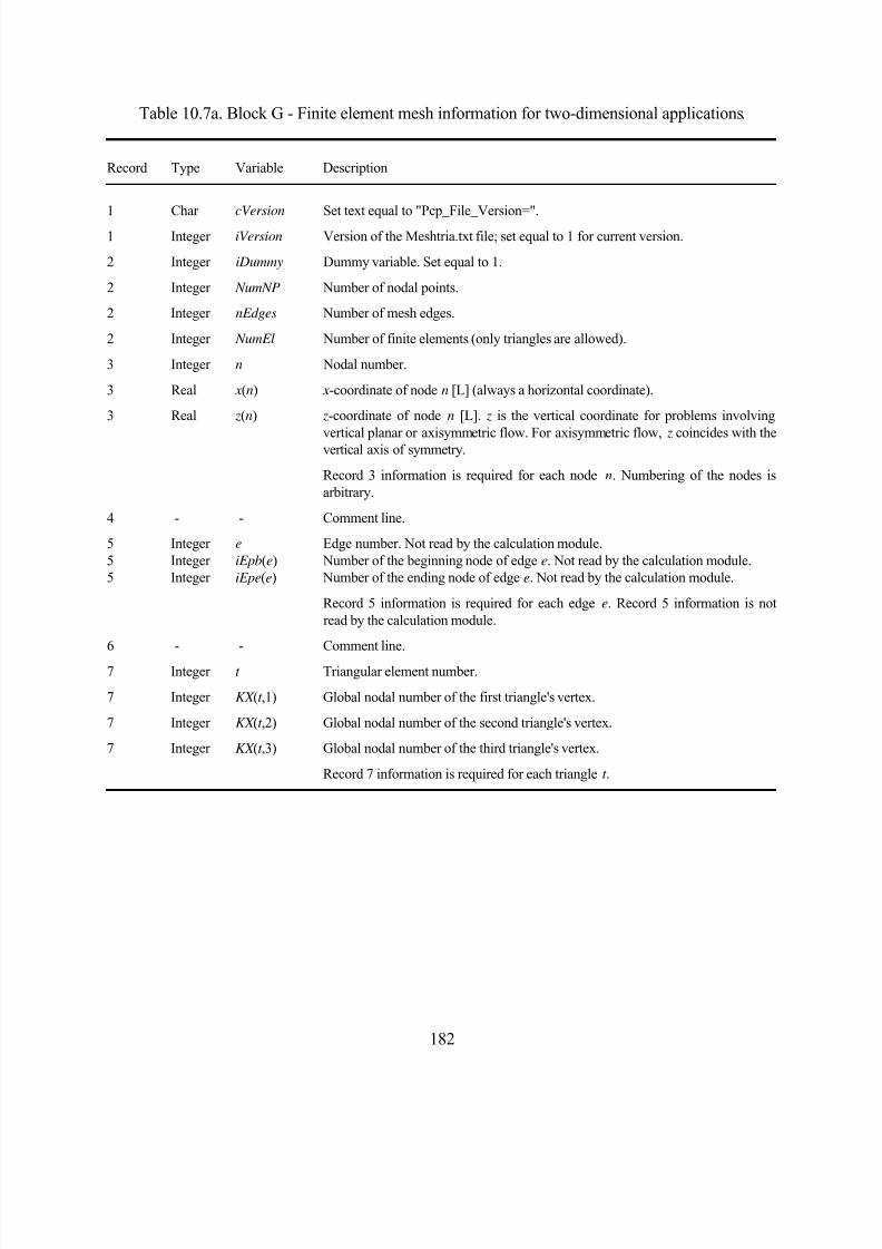
8/20/2019 HYDRUS3D Technical Manual.pdf
http://slidepdf.com/reader/full/hydrus3d-technical-manualpdf 212/260
182
Table 10.7a. Block G - Finite element mesh information for two-dimensional applications.
Record Type Variable Description
1 Char cVersion Set text equal to "Pcp_File_Version=".
1 Integer iVersion Version of the Meshtria.txt file; set equal to 1 for current version.
2 Integer iDummy Dummy variable. Set equal to 1.
2 Integer NumNP Number of nodal points.
2 Integer nEdges Number of mesh edges.
2 Integer NumEl Number of finite elements (only triangles are allowed).
3 Integer n Nodal number.
3 Real x(n) x-coordinate of node n [L] (always a horizontal coordinate).
3 Real z(n) z-coordinate of node n [L]. z is the vertical coordinate for problems involving
vertical planar or axisymmetric flow. For axisymmetric flow, z coincides with thevertical axis of symmetry.
Record 3 information is required for each node n. Numbering of the nodes isarbitrary.
4 - - Comment line.
5 Integer e Edge number. Not read by the calculation module.5 Integer iEpb(e) Number of the beginning node of edge e. Not read by the calculation module.5 Integer iEpe(e) Number of the ending node of edge e. Not read by the calculation module.
Record 5 information is required for each edge e. Record 5 information is notread by the calculation module.
6 - - Comment line.
7 Integer t Triangular element number.
7 Integer KX (t ,1) Global nodal number of the first triangle's vertex.
7 Integer KX (t ,2) Global nodal number of the second triangle's vertex.
7 Integer KX (t ,3) Global nodal number of the third triangle's vertex.
Record 7 information is required for each triangle t .
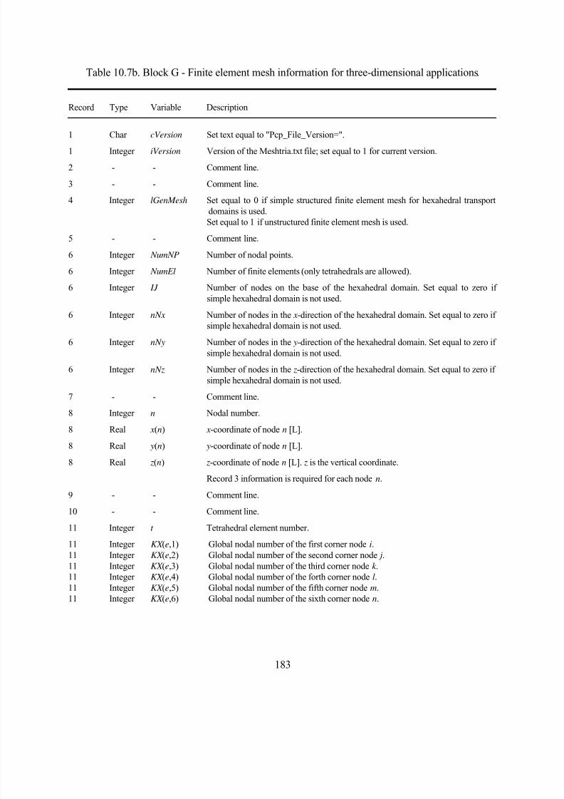
8/20/2019 HYDRUS3D Technical Manual.pdf
http://slidepdf.com/reader/full/hydrus3d-technical-manualpdf 213/260
183
Table 10.7b. Block G - Finite element mesh information for three-dimensional applications.
Record Type Variable Description
1 Char cVersion Set text equal to "Pcp_File_Version=".
1 Integer iVersion Version of the Meshtria.txt file; set equal to 1 for current version.
2 - - Comment line.
3 - - Comment line.
4 Integer lGenMesh Set equal to 0 if simple structured finite element mesh for hexahedral transportdomains is used.Set equal to 1 if unstructured finite element mesh is used.
5 - - Comment line.
6 Integer NumNP Number of nodal points.
6 Integer NumEl Number of finite elements (only tetrahedrals are allowed).
6 Integer IJ Number of nodes on the base of the hexahedral domain. Set equal to zero ifsimple hexahedral domain is not used.
6 Integer nNx Number of nodes in the x-direction of the hexahedral domain. Set equal to zero ifsimple hexahedral domain is not used.
6 Integer nNy Number of nodes in the y-direction of the hexahedral domain. Set equal to zero ifsimple hexahedral domain is not used.
6 Integer nNz Number of nodes in the z-direction of the hexahedral domain. Set equal to zero ifsimple hexahedral domain is not used.
7 - - Comment line.
8 Integer n Nodal number.
8 Real x(n) x-coordinate of node n [L].
8 Real y(n) y-coordinate of node n [L].
8 Real z(n) z-coordinate of node n [L]. z is the vertical coordinate.
Record 3 information is required for each node n.
9 - - Comment line.
10 - - Comment line.
11 Integer t Tetrahedral element number.
11 Integer KX (e,1) Global nodal number of the first corner node i.
11 Integer KX
(e,2) Global nodal number of the second corner node
j.11 Integer KX (e,3) Global nodal number of the third corner node k .
11 Integer KX (e,4) Global nodal number of the forth corner node l.11 Integer KX (e,5) Global nodal number of the fifth corner node m.11 Integer KX (e,6) Global nodal number of the sixth corner node n.

8/20/2019 HYDRUS3D Technical Manual.pdf
http://slidepdf.com/reader/full/hydrus3d-technical-manualpdf 214/260
184
Table 10.7b. (continued)
Record Type Variable Description
11 Integer KX (e,7) Global nodal number of the seventh corner node o.11 Integer KX (e,8) Global nodal number of the eighth corner node p. Indices i, j, k, l, m, n, o and p,refer to the corner nodes of an element e taken in a certain orientation asdescribed in Section 6.1. KX (e,5) for tetrahedral and KX (e,7) for triangular prismatic elements must be equal to zero.
11 Integer KX (e,9) Code specifying the subdivision of hexahedral and triangular prismatic elementsinto tetrahedrals (See Chapter 6.1 and Figure 6.1).
Record 11 information is required for each triangle t .
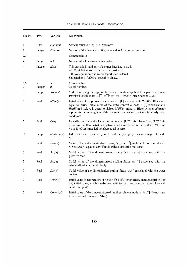
8/20/2019 HYDRUS3D Technical Manual.pdf
http://slidepdf.com/reader/full/hydrus3d-technical-manualpdf 215/260
185
Table 10.8. Block H - Nodal information.
Record Type Variable Description
1 Char cVersion Set text equal to "Pcp_File_Version=".
1 Integer iVersion Version of the Domain.dat file; set equal to 2 for current version.
2,3 - - Comment lines.
4 Integer NS Number of solutes in a chain reaction.
4 Integer iEquil This variable is read only if the user interface is used.= 1; Equilibrium solute transport is considered.= 0; Nonequilibrium solute transport is considered.Set equal to 1 if lChem is equal to .false..
5,6 - - Comment line.7 Integer n Nodal number.
7 Integer Kode(n) Code specifying the type of boundary condition applied to a particular node.Permissible values are 0, 1,±2, ±3, ±4,. .., ± NumKD (see Section 8.3).
7 Real hNew(n) Initial value of the pressure head at node n [L] when variable lInitW in Block A isequal to .true.. Initial value of the water content at node n [L] when variablelInitW in Block A is equal to .false.. If lWat =.false. in Block A, then hNew(n)represents the initial guess of the pressure head (water content) for steady stateconditions.
7 Real Q(n) Prescribed recharge/discharge rate at node n; [L2T-1] for planar flow, [L3T-1] foraxisymmetric flow. Q(n) is negative when directed out of the system. When novalue for Q(n) is needed, set Q(n) equal to zero.
7 Integer MatNum(n) Index for material whose hydraulic and transport properties are assigned to noden.
7 Real Beta(n) Value of the water uptake distribution, b( x,y,z) [L-2], in the soil root zone at noden. Set Beta(n) equal to zero if node n lies outside the root zone.
7 Real Axz(n) Nodal value of the dimensionless scaling factor α h [-] associated with the pressure head.
7 Real Bxz(n) Nodal value of the dimensionless scaling factor α K [-] associated with thesaturated hydraulic conductivity.
7 Real Dxz(n) Nodal value of the dimensionless scaling factor α θ [-] associated with the watercontent.
7 Real Temp(n) Initial value of temperature at node n [oC] (if lTemp=.false. then set equal to 0 orany initial value, which is to be used with temperature dependent water flow and
solute transport).
7 Real Conc(1,n) Initial value of the concentration of the first solute at node n [ML-3] (do not haveto be specified if lChem=.false.).
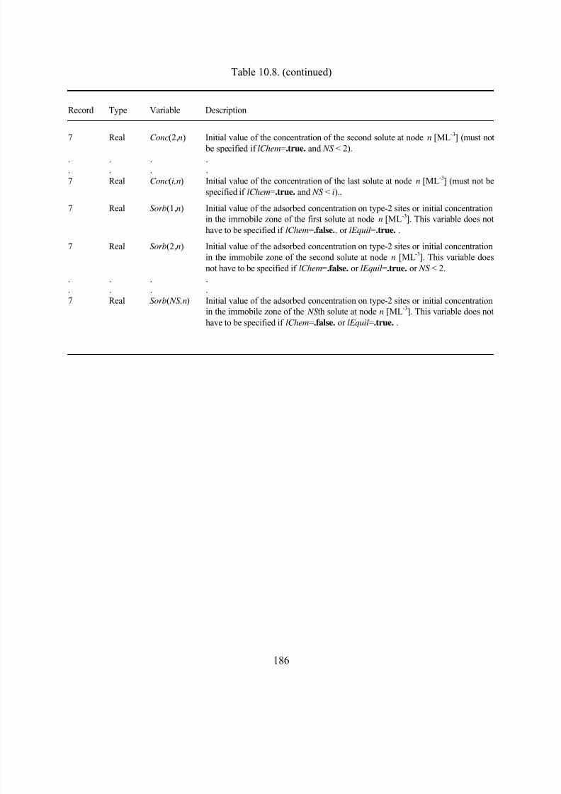
8/20/2019 HYDRUS3D Technical Manual.pdf
http://slidepdf.com/reader/full/hydrus3d-technical-manualpdf 216/260
186
Table 10.8. (continued)
Record Type Variable Description
7 Real Conc(2,n) Initial value of the concentration of the second solute at node n [ML-3
] (must not be specified if lChem=.true. and NS < 2).. . . .. . . .7 Real Conc(i,n) Initial value of the concentration of the last solute at node n [ML-3] (must not be
specified if lChem=.true. and NS < i)..
7 Real Sorb(1,n) Initial value of the adsorbed concentration on type-2 sites or initial concentrationin the immobile zone of the first solute at node n [ML-3]. This variable does nothave to be specified if lChem=.false.. or lEquil=.true. .
7 Real Sorb(2,n) Initial value of the adsorbed concentration on type-2 sites or initial concentrationin the immobile zone of the second solute at node n [ML-3]. This variable doesnot have to be specified if lChem=.false. or lEquil=.true. or NS < 2.
. . . .
. . . .7 Real Sorb( NS,n) Initial value of the adsorbed concentration on type-2 sites or initial concentration
in the immobile zone of the NS th solute at node n [ML-3]. This variable does nothave to be specified if lChem=.false. or lEquil=.true. .
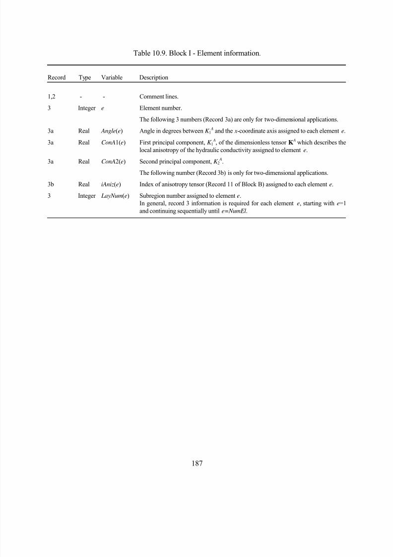
8/20/2019 HYDRUS3D Technical Manual.pdf
http://slidepdf.com/reader/full/hydrus3d-technical-manualpdf 217/260
187
Table 10.9. Block I - Element information.
Record Type Variable Description
1,2 - - Comment lines.3 Integer e Element number.
The following 3 numbers (Record 3a) are only for two-dimensional applications.
3a Real Angle(e) Angle in degrees between K 1 A and the x-coordinate axis assigned to each element e.
3a Real ConA1(e) First principal component, K 1 A, of the dimensionless tensor K
A which describes thelocal anisotropy of the hydraulic conductivity assigned to element e.
3a Real ConA2(e) Second principal component, K 2 A.
The following number (Record 3b) is only for two-dimensional applications.
3b Real iAniz(e) Index of anisotropy tensor (Record 11 of Block B) assigned to each element e.
3 Integer LayNum(e) Subregion number assigned to element e.In general, record 3 information is required for each element e, starting with e=1and continuing sequentially until e=NumEl.
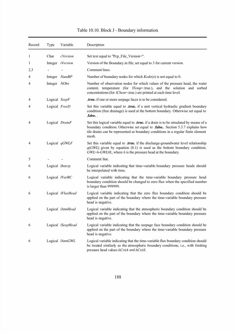
8/20/2019 HYDRUS3D Technical Manual.pdf
http://slidepdf.com/reader/full/hydrus3d-technical-manualpdf 218/260
188
Table 10.10. Block J - Boundary information.
Record Type Variable Description
1 Char cVersion Set text equal to "Pcp_File_Version=".
1 Integer iVersion Version of the Boundary.in file; set equal to 3 for current version.
2,3 - - Comment lines.
4 Integer NumBP Number of boundary nodes for which Kode(n) is not equal to 0.
4 Integer NObs Number of observation nodes for which values of the pressure head, the watercontent, temperature (for lTemp=.true.), and the solution and sorbedconcentrations (for lChem=.true.) are printed at each time level.
4 Logical SeepF .true. if one or more seepage faces is to be considered.
4 Logical FreeD Set this variable equal to .true. if a unit vertical hydraulic gradient boundarycondition (free drainage) is used at the bottom boundary. Otherwise set equal to
.false. .4 Logical DrainF Set this logical variable equal to .true. if a drain is to be simulated by means of a
boundary condition. Otherwise set equal to .false.. Section 5.3.7 explains howtile drains can be represented as boundary conditions in a regular finite elementmesh.
4 Logical qGWLF Set this variable equal to .true. if the discharge-groundwater level relationshipq(GWL) given by equation (8.1) is used as the bottom boundary condition; GWL=h-GWL0L, where h is the pressure head at the boundary.
5 - - Comment line.
6 Logical lInterp Logical variable indicating that time-variable boundary pressure heads should be interpolated with time.
6 Logical lVarBC Logical variable indicating that the time-variable boundary pressure head boundary condition should be changed to zero flux when the specified numberis larger than 999999.
6 Logical lFluxHead Logical variable indicating that the zero flux boundary condition should beapplied on the part of the boundary where the time-variable boundary pressurehead is negative.
6 Logical lAtmHead Logical variable indicating that the atmospheric boundary condition should beapplied on the part of the boundary where the time-variable boundary pressurehead is negative.
6 Logical lSeepHead Logical variable indicating that the seepage face boundary condition should beapplied on the part of the boundary where the time-variable boundary pressure
head is negative.6 Logical lAtmGWL Logical variable indicating that the time-variable flux boundary condition should
be treated similarly as the atmospheric boundary conditions, i.e., with limiting pressure head values hCritA and hCritS .
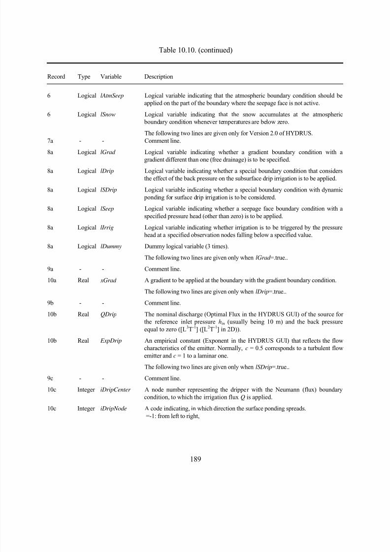
8/20/2019 HYDRUS3D Technical Manual.pdf
http://slidepdf.com/reader/full/hydrus3d-technical-manualpdf 219/260
189
Table 10.10. (continued)
Record Type Variable Description
6 Logical lAtmSeep Logical variable indicating that the atmospheric boundary condition should beapplied on the part of the boundary where the seepage face is not active.
6 Logical lSnow Logical variable indicating that the snow accumulates at the atmospheric boundary condition whenever temperatures are below zero.
The following two lines are given only for Version 2.0 of HYDRUS.7a - - Comment line.
8a Logical lGrad Logical variable indicating whether a gradient boundary condition with agradient different than one (free drainage) is to be specified.
8a Logical lDrip Logical variable indicating whether a special boundary condition that considersthe effect of the back pressure on the subsurface drip irrigation is to be applied.
8a Logical lSDrip Logical variable indicating whether a special boundary condition with dynamic ponding for surface drip irrigation is to be considered.
8a Logical lSeep Logical variable indicating whether a seepage face boundary condition with aspecified pressure head (other than zero) is to be applied.
8a Logical lIrrig Logical variable indicating whether irrigation is to be triggered by the pressurehead at a specified observation nodes falling below a specified value.
8a Logical lDummy Dummy logical variable (3 times).
The following two lines are given only when lGrad =.true..
9a - - Comment line.
10a Real xGrad A gradient to be applied at the boundary with the gradient boundary condition.
The following two lines are given only when lDrip=.true..
9b - - Comment line.
10b Real QDrip The nominal discharge (Optimal Flux in the HYDRUS GUI) of the source forthe reference inlet pressure hin (usually being 10 m) and the back pressureequal to zero ([L3T-1] ([L2T-1] in 2D)).
10b Real ExpDrip An empirical constant (Exponent in the HYDRUS GUI) that reflects the flowcharacteristics of the emitter. Normally, c = 0.5 corresponds to a turbulent flowemitter and c = 1 to a laminar one.
The following two lines are given only when lSDrip=.true..
9c - - Comment line.
10c Integer iDripCenter A node number representing the dripper with the Neumann (flux) boundarycondition, to which the irrigation flux Q is applied.
10c Integer iDripNode A code indicating, in which direction the surface ponding spreads.=-1: from left to right,
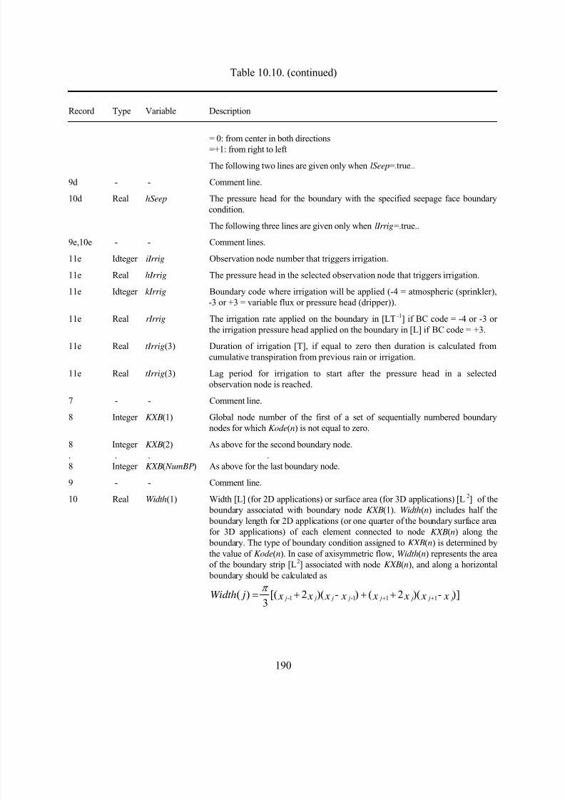
8/20/2019 HYDRUS3D Technical Manual.pdf
http://slidepdf.com/reader/full/hydrus3d-technical-manualpdf 220/260
190
Table 10.10. (continued)
Record Type Variable Description
= 0: from center in both directions=+1: from right to left
The following two lines are given only when lSeep=.true..
9d - - Comment line.
10d Real hSeep The pressure head for the boundary with the specified seepage face boundarycondition.
The following three lines are given only when lIrrig=.true..
9e,10e - - Comment lines.
11e Idteger iIrrig Observation node number that triggers irrigation.
11e Real hIrrig The pressure head in the selected observation node that triggers irrigation.
11e Idteger kIrrig Boundary code where irrigation will be applied (-4 = atmospheric (sprinkler),-3 or +3 = variable flux or pressure head (dripper)).
11e Real rIrrig The irrigation rate applied on the boundary in [LT-1] if BC code = -4 or -3 orthe irrigation pressure head applied on the boundary in [L] if BC code = +3.
11e Real tIrrig(3) Duration of irrigation [T], if equal to zero then duration is calculated fromcumulative transpiration from previous rain or irrigation.
11e Real tIrrig(3) Lag period for irrigation to start after the pressure head in a selectedobservation node is reached.
7 - - Comment line.
8 Integer KXB(1) Global node number of the first of a set of sequentially numbered boundarynodes for which Kode(n) is not equal to zero.
8 Integer KXB(2) As above for the second boundary node.. . . .8 Integer KXB( NumBP) As above for the last boundary node.
9 - - Comment line.
10 Real Width(1) Width [L] (for 2D applications) or surface area (for 3D applications) [L2] of the boundary associated with boundary node KXB(1). Width(n) includes half the boundary length for 2D applications (or one quarter of the boundary surface areafor 3D applications) of each element connected to node KXB(n) along the boundary. The type of boundary condition assigned to KXB(n) is determined bythe value of Kode(n). In case of axisymmetric flow, Width(n) represents the areaof the boundary strip [L2] associated with node KXB(n), and along a horizontal boundary should be calculated as
-1 -1 1 1( ) [( 2 )( - ) ( 2 )( - )]3
j j j j j j j jWidth j x x x x x x x xπ
+ += + + +
8/20/2019 HYDRUS3D Technical Manual.pdf
http://slidepdf.com/reader/full/hydrus3d-technical-manualpdf 221/260
8/20/2019 HYDRUS3D Technical Manual.pdf
http://slidepdf.com/reader/full/hydrus3d-technical-manualpdf 222/260
192
Table 10.10. (continued)
Record Type Variable Description
Records 17 through 19 are provided only for two-dimensional applications and when particle option is enabled.20,21 - - Comment lines.
22 Integer NSeep Number of seepage faces expected to develop.
23 - - Comment line.
24 Integer NSP(1) Number of nodes on the first seepage face.24 Integer NSP(2) Number of nodes on the second seepage face.. . . .. . . .24 Integer NSP( NSeep) Number of nodes on the last seepage face.
25 - - Comment line.
26 Integer NP(1,1) Sequential global number of the first node on the first seepage face.26 Integer NP(1,2) Sequential global number of the second node on the first seepage face.. . . .. . . .26 Integer NP(1, NSP(1)) Sequential global number of the last node on the first seepage face.
Record 26 information is provided for each seepage face.Records 20 through 26 information is not provided if the logical variable SeepF is set equal to .false. .
27,28 - - Comment lines.
29 Integer NDr Number of drains. See Section 5.3.7 for a discussion on how tile drains can berepresented as boundary conditions in a regular finite element mesh.
29 Real DrCorr Additional reduction in the correction factor C d (See Section 5.3.7).
30 - - Comment line.
31 Integer ND(1) Global number of the first drain.31 Integer ND(2) Global number of the second drain.. . . .. . . .31 Integer ND( NDr ) Global number of the last drain.
32 - - Comment line.
33 Integer NElD(1) Number of elements surrounding the first drain.33 Integer NElD(2) Number of elements surrounding the second drain.. . . .. . . .33 Integer NElD( NDr ) Number of elements surrounding the last drain.
34 - - Comment line.
8/20/2019 HYDRUS3D Technical Manual.pdf
http://slidepdf.com/reader/full/hydrus3d-technical-manualpdf 223/260
193
Table 10.10. (continued)
Record Type Variable Description
35 Real EfDim(1,1) Effective diameter of the first drain, d e [L] (see Section 5.3.7).35 Real EfDim(2,1) Dimension of the square in finite element mesh representing the first drain, D [L](see Section 5.3.7).
Record 35 information is provided for each drain.
36 - - Comment line.
37 Integer KElDr (1,1) Global number of the first element surrounding the first drain.37 Integer KElDr (1,2) Global number of the second element surrounding the first drain.. . . .. . . .37 Integer KElDr (1, NElD(1)) Global number of the last element surrounding the first drain.
Record 37 information is provided for each drain.
Records 27 through 37 are provided only if the logical variable DrainF is setequal to .true. .
38,39 - - Comment lines.
40 Integer KodCB(1) Code specifying the type of boundary condition for solute transport applied to a particular node. Positive and negative signs indicate that first-, or second- orthird- (depending upon the calculated water flux Q), type boundary conditionsare implemented, respectively. In case of time-independent boundary conditions(Kode(1)= ±1, ±2, ±5, or ±6; See Block H), KodCB(1) also refers to the fieldcBound for the value of the solute transport BC. cBound (i,abs(KodCB(1))) is thevalue of the boundary condition for node KXB(1) (the first of a set ofsequentially numbered boundary nodes for which Kode( N ) is not equal to zero).Permissible values are ±1, ±2,..., ±5, ±6,-7. When KodCB(1) equals -7, a special
type of boundary condition for volatile solutes described by equations (3.45) and(3.46) is applied.
40 Integer KodCB(2) Same as above for the second boundary node.. . . .. . . .40 Integer KodCB( NumBP) Same as above for the last boundary node.
Records 38 through 40 are provided only if the logical variable lChem (Block A)is set equal to .true. .
41,42 - - Comment line.
8/20/2019 HYDRUS3D Technical Manual.pdf
http://slidepdf.com/reader/full/hydrus3d-technical-manualpdf 224/260
194
Table 10.10. (continued)
Record Type Variable Description
243 Integer KodTB(1) Code specifying the type of boundary condition for heat transport applied to a particular node. Positive and negative signs mean that first-, or second- or third-(depending upon the calculated water flux Q) type boundary conditions will beimplemented, respectively. In case of time-independent boundary conditions(Kode(1)= ±1, ±2, ±5, or ±6; See Block H), KodTB(1) refers to the vectorTBound for the value of the heat transport BC. TBound (abs(KodTB(1))) is thevalue of the boundary condition for node KXB(1) (the first of a set ofsequentially numbered boundary nodes for which Kode( N ) is not equal to zero).Permissible values are ±1,..., ±6.
43 Integer KodTB(2) Same as above for the second boundary node.. . . .. . . .43 Integer KodTB( NumBP) Same as above for the last boundary node.
Records 41 through 43 are provided only if the logical variable lTemp (Block A)is set equal to .true. .
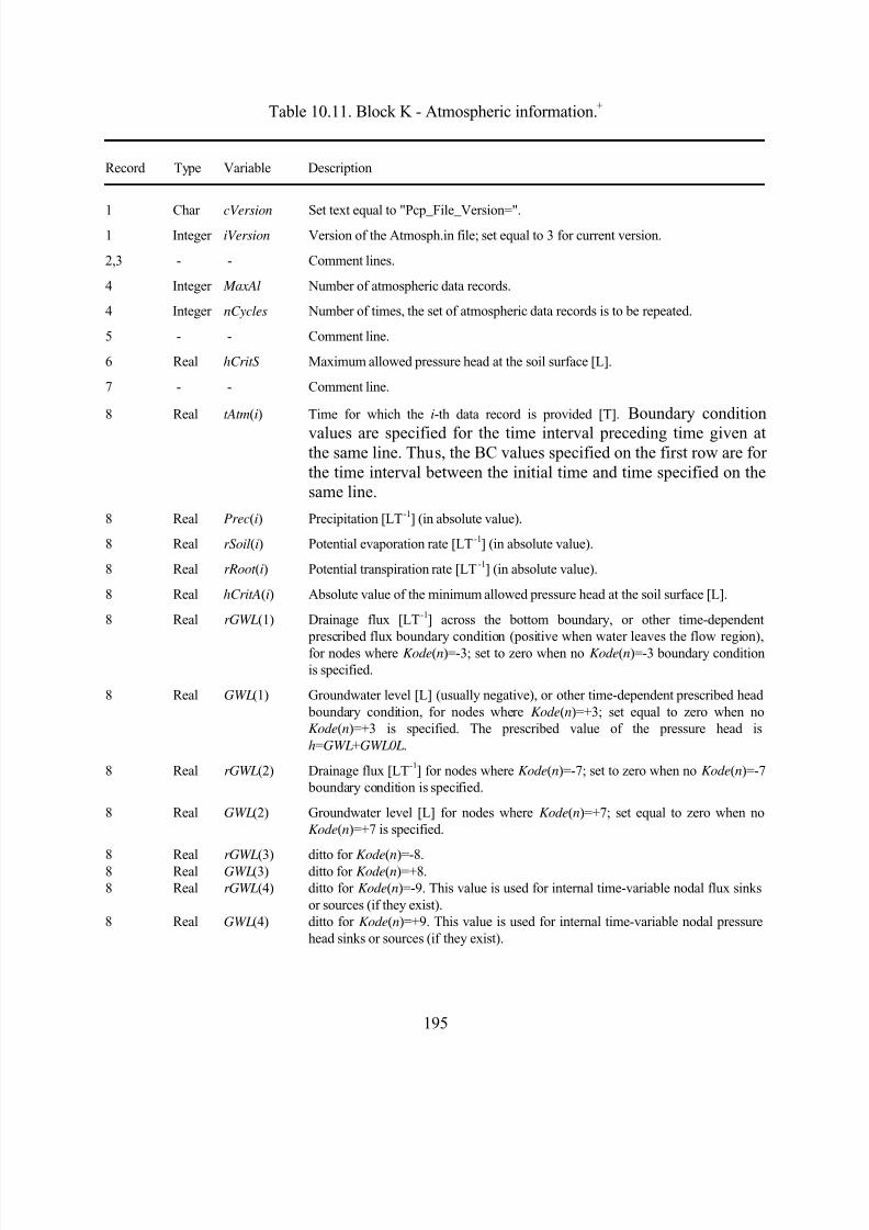
8/20/2019 HYDRUS3D Technical Manual.pdf
http://slidepdf.com/reader/full/hydrus3d-technical-manualpdf 225/260
195
Table 10.11. Block K - Atmospheric information.+
Record Type Variable Description
1 Char cVersion Set text equal to "Pcp_File_Version=".1 Integer iVersion Version of the Atmosph.in file; set equal to 3 for current version.
2,3 - - Comment lines.
4 Integer MaxAl Number of atmospheric data records.
4 Integer nCycles Number of times, the set of atmospheric data records is to be repeated.
5 - - Comment line.
6 Real hCritS Maximum allowed pressure head at the soil surface [L].
7 - - Comment line.
8 Real tAtm(i) Time for which the i-th data record is provided [T]. Boundary condition
values are specified for the time interval preceding time given atthe same line. Thus, the BC values specified on the first row are forthe time interval between the initial time and time specified on thesame line.
8 Real Prec(i) Precipitation [LT-1] (in absolute value).
8 Real rSoil(i) Potential evaporation rate [LT-1] (in absolute value).
8 Real rRoot (i) Potential transpiration rate [LT-1] (in absolute value).
8 Real hCritA(i) Absolute value of the minimum allowed pressure head at the soil surface [L].
8 Real rGWL(1) Drainage flux [LT-1] across the bottom boundary, or other time-dependent prescribed flux boundary condition (positive when water leaves the flow region),for nodes where Kode(n)=-3; set to zero when no Kode(n)=-3 boundary conditionis specified.
8 Real GWL(1) Groundwater level [L] (usually negative), or other time-dependent prescribed head boundary condition, for nodes where Kode(n)=+3; set equal to zero when noKode(n)=+3 is specified. The prescribed value of the pressure head ish=GWL+GWL0L.
8 Real rGWL(2) Drainage flux [LT-1] for nodes where Kode(n)=-7; set to zero when no Kode(n)=-7 boundary condition is specified.
8 Real GWL(2) Groundwater level [L] for nodes where Kode(n)=+7; set equal to zero when noKode(n)=+7 is specified.
8 Real rGWL
(3) ditto forKode
(n
)=-8.8 Real GWL(3) ditto for Kode(n)=+8.8 Real rGWL(4) ditto for Kode(n)=-9. This value is used for internal time-variable nodal flux sinks
or sources (if they exist).8 Real GWL(4) ditto for Kode(n)=+9. This value is used for internal time-variable nodal pressure
head sinks or sources (if they exist).
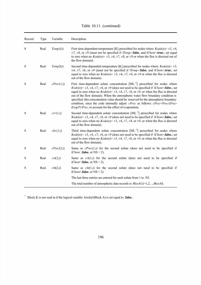
8/20/2019 HYDRUS3D Technical Manual.pdf
http://slidepdf.com/reader/full/hydrus3d-technical-manualpdf 226/260
196
Table 10.11. (continued)
Record Type Variable Description
8 Real Temp1(i) First time-dependent temperature [K] prescribed for nodes where Kode(n)= ±3, ±4,±7, ±8, or ±9 (must not be specified if lTemp=.false. and lChem=.true.; set equalto zero when no Kode(n)= ±3, ±4, ±7, ±8, or ±9 or when the flux is directed out ofthe flow domain).
8 Real Temp2(i) Second time-dependent temperature [K] prescribed for nodes where Kode(n)= ±3,±4, ±7, ±8, or ±9 (must not be specified if lTemp=.false. and lChem=.true.; setequal to zero when no Kode(n)= ±3, ±4, ±7, ±8, or ±9 or when the flux is directedout of the flow domain).
8 Real cPrec(1,i) First time-dependent solute concentration [ML-3] prescribed for nodes whereKode(n)= ±3, ±4, ±7, ±8, or ±9 (does not need to be specified if lChem=.false.; setequal to zero when no Kode(n)= ±3, ±4, ±7, ±8, or ±9, or when the flux is directedout of the flow domain). When the atmospheric water flow boundary condition is
specified, this concentration value should be reserved for the atmospheric boundarycondition, since the code internally adjust cPrec as follows: cPrec=Prec/(Prec-Evap)*cPrec, to account for the effect of evaporation.
8 Real crt (1,i) Second time-dependent solute concentration [ML-3] prescribed for nodes whereKode(n)= ±3, ±4, ±7, ±8, or ±9 (does not need to be specified if lChem=.false.; setequal to zero when no Kode(n)= ±3, ±4, ±7, ±8, or ±9, or when the flux is directedout of the flow domain).
8 Real cht (1,i) Third time-dependent solute concentration [ML-3] prescribed for nodes whereKode(n)= ±3, ±4, ±7, ±8, or ±9 (does not need to be specified if lChem=.false.; setequal to zero when no Kode(n)= ±3, ±4, ±7, ±8, or ±9, or when the flux is directedout of the flow domain).
8 Real cPrec(2,i) Same as cPrec(1,i) for the second solute (does not need to be specified iflChem=.false. or NS < 2).
8 Real crt (2,i) Same as crt (1,i) for the second solute (does not need to be specified iflChem=.false. or NS < 2).
8 Real cht (2,i) Same as cht (1,i) for the second solute (does not need to be specified iflChem=.false. or NS < 2).
The last three entries are entered for each solute from 1 to NS .
The total number of atmospheric data records is MaxAl (i=1,2, .., MaxAl).
+ Block K is not read in if the logical variable AtmInf (Block A) is set equal to .false. .
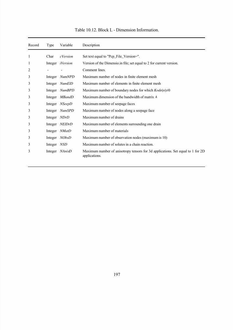
8/20/2019 HYDRUS3D Technical Manual.pdf
http://slidepdf.com/reader/full/hydrus3d-technical-manualpdf 227/260
197
Table 10.12. Block L - Dimension Information.
Record Type Variable Description
1 Char cVersion Set text equal to "Pcp_File_Version=".1 Integer iVersion Version of the Dimensio.in file; set equal to 2 for current version.
2 - - Comment lines.
3 Integer NumNPD Maximum number of nodes in finite element mesh
3 Integer NumElD Maximum number of elements in finite element mesh
3 Integer NumBPD Maximum number of boundary nodes for which Kode(n)≠0
3 Integer MBandD Maximum dimension of the bandwidth of matrix A
3 Integer NSeepD Maximum number of seepage faces
3 Integer NumSPD Maximum number of nodes along a seepage face
3 Integer NDrD Maximum number of drains
3 Integer NElDrD Maximum number of elements surrounding one drain
3 Integer NMatD Maximum number of materials
3 Integer NObsD Maximum number of observation nodes (maximum is 10)
3 Integer NSD Maximum number of solutes in a chain reaction.
3 Integer NAnisD Maximum number of anisotropy tensors for 3d applications. Set equal to 1 for 2Dapplications.
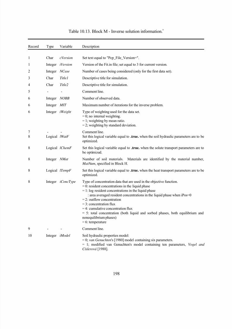
8/20/2019 HYDRUS3D Technical Manual.pdf
http://slidepdf.com/reader/full/hydrus3d-technical-manualpdf 228/260
198
Table 10.13. Block M - Inverse solution information.+
Record Type Variable Description
1 Char cVersion Set text equal to "Pcp_File_Version=".1 Integer iVersion Version of the Fit.in file; set equal to 3 for current version.
2 Integer NCase Number of cases being considered (only for the first data set).
3 Char Title1 Descriptive title for simulation.
4 Char Title2 Descriptive title for simulation.
5 - - Comment line.
6 Integer NOBB Number of observed data.
6 Integer MIT Maximum number of iterations for the inverse problem.
6 Integer iWeight Type of weighting used for the data set.
= 0; no internal weighting.= 1; weighting by mean ratio.= 2; weighting by standard deviation.
7 - - Comment line.8 Logical lWatF Set this logical variable equal to .true. when the soil hydraulic parameters are to be
optimized.
8 Logical lChemF Set this logical variable equal to .true. when the solute transport parameters are to be optimized.
8 Integer NMat Number of soil materials. Materials are identified by the material number, MatNum, specified in Block H.
8 Logical lTempF Set this logical variable equal to .true. when the heat transport parameters are to beoptimized.
8 Integer iConcType Type of concentration data that are used in the objective function.= 0: resident concentrations in the liquid phase= 1: log resident concentrations in the liquid phase
: area averaged resident concentrations in the liquid phase when iPos=0= 2: outflow concentration= 3: concentration flux= 4: cumulative concentration flux= 5: total concentration (both liquid and sorbed phases, both equilibrium andnonequilibrium phases)= 6: temperature
9 - - Comment line.10 Integer iModel Soil hydraulic properties model:
= 0; van Genuchten's [1980] model containing six parameters.= 1; modified van Genuchten's model containing ten parameters, Vogel andCíslerová [1988].
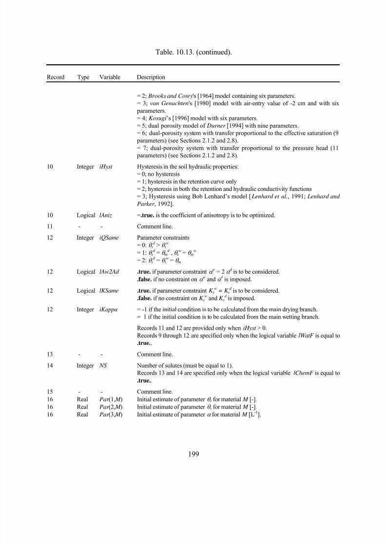
8/20/2019 HYDRUS3D Technical Manual.pdf
http://slidepdf.com/reader/full/hydrus3d-technical-manualpdf 229/260
199
Table. 10.13. (continued).
Record Type Variable Description
= 2; Brooks and Corey's [1964] model containing six parameters.= 3; van Genuchten's [1980] model with air-entry value of -2 cm and with six parameters.= 4; Kosugi’s [1996] model with six parameters.= 5; dual porosity model of Durner [1994] with nine parameters.= 6; dual-porosity system with transfer proportional to the effective saturation (9 parameters) (see Sections 2.1.2 and 2.8).= 7; dual-porosity system with transfer proportional to the pressure head (11 parameters) (see Sections 2.1.2 and 2.8).
10 Integer iHyst Hysteresis in the soil hydraulic properties:= 0; no hysteresis= 1; hysteresis in the retention curve only
= 2; hysteresis in both the retention and hydraulic conductivity functions= 3; Hysteresis using Bob Lenhard’s model [ Lenhard et al., 1991; Lenhard andParker , 1992].
10 Logical lAniz =.true. is the coefficient of anisotropy is to be optimized.
11 - - Comment line.
12 Integer iQSame Parameter constraints= 0: θ s
d > θ sw
= 1: θ sd = θ m
d , θ sw = θ m
w = 2: θ s
d = θ sw = θ m
12 Logical lAw2Ad .true. if parameter constraint α w = 2 α d is to be considered..false. if no constraint on α
w and α d is imposed.
12 Logical lKSame .true. if parameter constraint K sw = K sd is to be considered..false. if no constraint on K s
w and K sd is imposed.
12 Integer iKappa = -1 if the initial condition is to be calculated from the main drying branch.= 1 if the initial condition is to be calculated from the main wetting branch.
Records 11 and 12 are provided only when iHyst > 0.Records 9 through 12 are specified only when the logical variable lWatF is equal to.true..
13 - - Comment line.
14 Integer NS Number of solutes (must be equal to 1).Records 13 and 14 are specified only when the logical variable lChemF is equal to
.true..15 - - Comment line.16 Real Par (1, M ) Initial estimate of parameter θ r for material M [-].16 Real Par (2, M ) Initial estimate of parameter θ s for material M [-].16 Real Par (3, M ) Initial estimate of parameter α for material M [L-1].
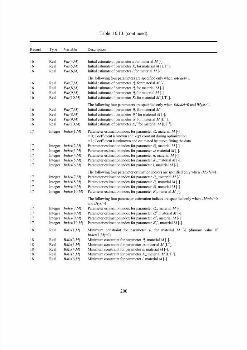
8/20/2019 HYDRUS3D Technical Manual.pdf
http://slidepdf.com/reader/full/hydrus3d-technical-manualpdf 230/260
200
Table. 10.13. (continued).
Record Type Variable Description
16 Real Par (4, M ) Initial estimate of parameter n for material M [-].16 Real Par (5, M ) Initial estimate of parameter K s for material M [LT-1].16 Real Par (6, M ) Initial estimate of parameter l for material M [-].
The following four parameters are specified only when iModel=1.16 Real Par (7, M ) Initial estimate of parameter θ m for material M [-].16 Real Par (8, M ) Initial estimate of parameter θ a for material M [-].16 Real Par (9, M ) Initial estimate of parameter θ k for material M [-].16 Real Par (10, M ) Initial estimate of parameter K k for material M [LT-1].
The following four parameters are specified only when iModel=0 and iHyst >1.16 Real Par (7, M ) Initial estimate of parameter θ m for material M [-].16 Real Par (8, M ) Initial estimate of parameter θ s
w for material M [-].16 Real Par (9, M ) Initial estimate of parameter α w for material M [L-1].16 Real Par (10, M ) Initial estimate of parameter K sw for material M [LT-1].
17 Integer Index(1, M ) Parameter estimation index for parameter θ r , material M [-].= 0; Coefficient is known and kept constant during optimization.= 1; Coefficient is unknown and estimated by curve fitting the data.
17 Integer Index(2, M ) Parameter estimation index for parameter θ s, material M [-].17 Integer Index(3, M ) Parameter estimation index for parameter α , material M [-].17 Integer Index(4, M ) Parameter estimation index for parameter n, material M [-].17 Integer Index(5, M ) Parameter estimation index for parameter K s, material M [-].17 Integer Index(6, M ) Parameter estimation index for parameter l, material M [-].
The following four parameter estimation indices are specified only when iModel=1.17 Integer Index(7, M ) Parameter estimation index for parameter θ m, material M [-].
17 Integer Index
(8, M
) Parameter estimation index for parameterθ
a, material M
[-].17 Integer Index(9, M ) Parameter estimation index for parameter θ k , material M [-].17 Integer Index(10, M ) Parameter estimation index for parameter K k , material M [-].
The following four parameter estimation indices are specified only when iModel=0and iHyst >1.
17 Integer Index(7, M ) Parameter estimation index for parameter θ m, material M [-].17 Integer Index(8, M ) Parameter estimation index for parameter θ s
w, material M [-].17 Integer Index(9, M ) Parameter estimation index for parameter α
w, material M [-].17 Integer Index(10, M ) Parameter estimation index for parameter K s
w, material M [-].
18 Real BMn(1, M ) Minimum constraint for parameter θ r for material M [-] (dummy value if Index(1, M )=0).
18 Real BMn(2, M ) Minimum constraint for parameter θ s, material M [-].
18 Real BMn(3, M ) Minimum constraint for parameter α , material M [L-1
].18 Real BMn(4, M ) Minimum constraint for parameter n, material M [-].18 Real BMn(5, M ) Minimum constraint for parameter K s, material M [LT-1].18 Real BMn(6, M ) Minimum constraint for parameter l, material M [-].
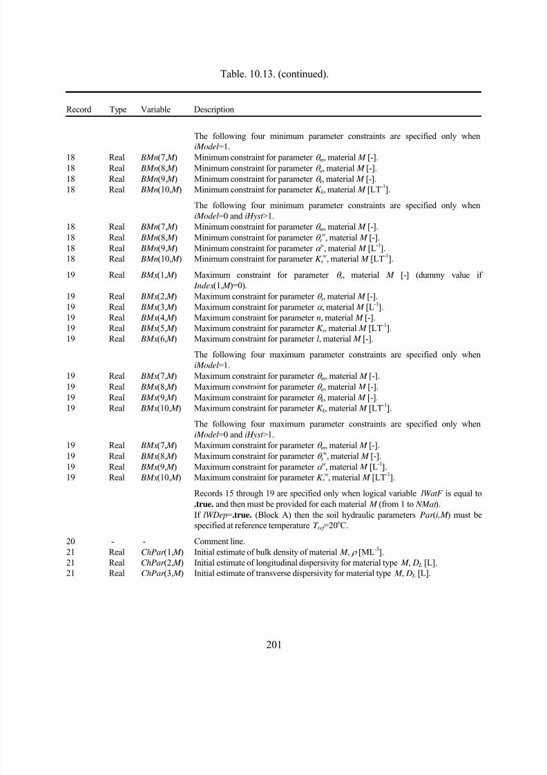
8/20/2019 HYDRUS3D Technical Manual.pdf
http://slidepdf.com/reader/full/hydrus3d-technical-manualpdf 231/260
201
Table. 10.13. (continued).
Record Type Variable Description
The following four minimum parameter constraints are specified only wheniModel=1.
18 Real BMn(7, M ) Minimum constraint for parameter θ m, material M [-].18 Real BMn(8, M ) Minimum constraint for parameter θ a, material M [-].18 Real BMn(9, M ) Minimum constraint for parameter θ k , material M [-].18 Real BMn(10, M ) Minimum constraint for parameter K k , material M [LT-1].
The following four minimum parameter constraints are specified only wheniModel=0 and iHyst >1.
18 Real BMn(7, M ) Minimum constraint for parameter θ m, material M [-].18 Real BMn(8, M ) Minimum constraint for parameter θ s
w, material M [-].18 Real BMn(9, M ) Minimum constraint for parameter α w, material M [L-1].18 Real BMn(10, M ) Minimum constraint for parameter K s
w, material M [LT-1].
19 Real BMx(1, M ) Maximum constraint for parameter θ r , material M [-] (dummy value if Index(1, M )=0).
19 Real BMx(2, M ) Maximum constraint for parameter θ s, material M [-].19 Real BMx(3, M ) Maximum constraint for parameter α , material M [L-1].19 Real BMx(4, M ) Maximum constraint for parameter n, material M [-].19 Real BMx(5, M ) Maximum constraint for parameter K s, material M [LT-1].19 Real BMx(6, M ) Maximum constraint for parameter l, material M [-].
The following four maximum parameter constraints are specified only wheniModel=1.
19 Real BMx(7, M ) Maximum constraint for parameter θ m, material M [-].19 Real BMx(8, M ) Maximum constraint for parameter θ a, material M [-].19 Real BMx(9, M ) Maximum constraint for parameter θ k , material M [-].
19 Real BMx(10, M ) Maximum constraint for parameter K k , material M [LT-1].The following four maximum parameter constraints are specified only wheniModel=0 and iHyst >1.
19 Real BMx(7, M ) Maximum constraint for parameter θ m, material M [-].19 Real BMx(8, M ) Maximum constraint for parameter θ s
w, material M [-].19 Real BMx(9, M ) Maximum constraint for parameter α w, material M [L-1].19 Real BMx(10, M ) Maximum constraint for parameter K s
w, material M [LT-1].
Records 15 through 19 are specified only when logical variable lWatF is equal to.true. and then must be provided for each material M (from 1 to NMat ).If lWDep=.true. (Block A) then the soil hydraulic parameters Par (i,M ) must bespecified at reference temperature T ref =20oC.
20 - - Comment line.21 Real ChPar (1, M ) Initial estimate of bulk density of material M , ρ [ML-3].21 Real ChPar (2, M ) Initial estimate of longitudinal dispersivity for material type M , D L [L].21 Real ChPar (3, M ) Initial estimate of transverse dispersivity for material type M , D L [L].
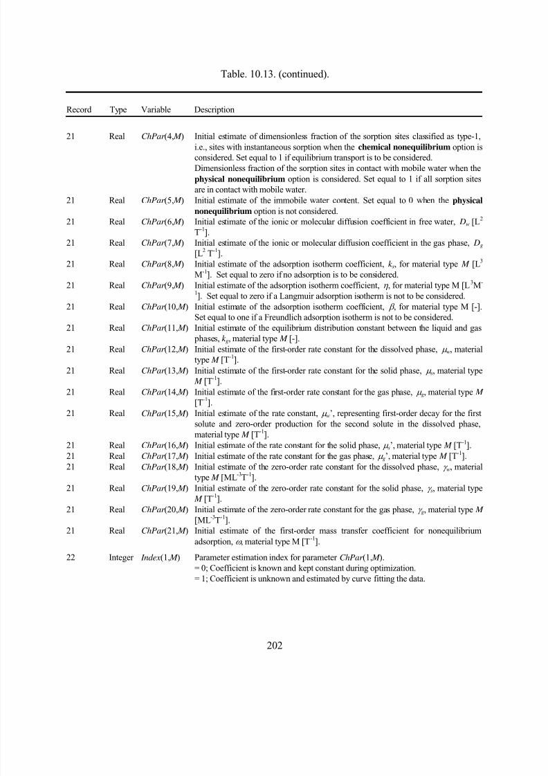
8/20/2019 HYDRUS3D Technical Manual.pdf
http://slidepdf.com/reader/full/hydrus3d-technical-manualpdf 232/260
202
Table. 10.13. (continued).
Record Type Variable Description
21 Real ChPar (4, M ) Initial estimate of dimensionless fraction of the sorption sites classified as type-1,i.e., sites with instantaneous sorption when the chemical nonequilibrium option isconsidered. Set equal to 1 if equilibrium transport is to be considered.Dimensionless fraction of the sorption sites in contact with mobile water when thephysical nonequilibrium option is considered. Set equal to 1 if all sorption sitesare in contact with mobile water.
21 Real ChPar (5, M ) Initial estimate of the immobile water content. Set equal to 0 when the physical
nonequilibrium option is not considered.21 Real ChPar (6, M ) Initial estimate of the ionic or molecular diffusion coefficient in free water, Dw [L2
T-1].21 Real ChPar (7, M ) Initial estimate of the ionic or molecular diffusion coefficient in the gas phase, Dg
[L2 T-1].21 Real ChPar (8, M ) Initial estimate of the adsorption isotherm coefficient, k s, for material type M [L3
M-1]. Set equal to zero if no adsorption is to be considered.21 Real ChPar (9, M ) Initial estimate of the adsorption isotherm coefficient, η , for material type M [L3M-
1]. Set equal to zero if a Langmuir adsorption isotherm is not to be considered.21 Real ChPar (10, M ) Initial estimate of the adsorption isotherm coefficient, β , for material type M [-].
Set equal to one if a Freundlich adsorption isotherm is not to be considered.21 Real ChPar (11, M ) Initial estimate of the equilibrium distribution constant between the liquid and gas
phases, k g, material type M [-].21 Real ChPar (12, M ) Initial estimate of the first-order rate constant for the dissolved phase, µ w, material
type M [T-1].21 Real ChPar (13, M ) Initial estimate of the first-order rate constant for the solid phase, µ s, material type
M [T-1].21 Real ChPar (14, M ) Initial estimate of the first-order rate constant for the gas phase, µ g, material type M
[T-1].21 Real ChPar (15, M ) Initial estimate of the rate constant, µ w’, representing first-order decay for the first
solute and zero-order production for the second solute in the dissolved phase,material type M [T-1].
21 Real ChPar (16, M ) Initial estimate of the rate constant for the solid phase, µ s’, material type M [T-1].21 Real ChPar (17, M ) Initial estimate of the rate constant for the gas phase, µ g’, material type M [T-1].21 Real ChPar (18, M ) Initial estimate of the zero-order rate constant for the dissolved phase, γ w, material
type M [ML-3T-1].21 Real ChPar (19, M ) Initial estimate of the zero-order rate constant for the solid phase, γ s, material type
M [T-1].21 Real ChPar (20, M ) Initial estimate of the zero-order rate constant for the gas phase, γ g, material type M
[ML-3T-1].21 Real ChPar (21, M ) Initial estimate of the first-order mass transfer coefficient for nonequilibrium
adsorption, ω , material type M [T-1
].22 Integer Index(1, M ) Parameter estimation index for parameter ChPar (1, M ).
= 0; Coefficient is known and kept constant during optimization.= 1; Coefficient is unknown and estimated by curve fitting the data.
8/20/2019 HYDRUS3D Technical Manual.pdf
http://slidepdf.com/reader/full/hydrus3d-technical-manualpdf 233/260
203
Table. 10.13. (continued).
Record Type Variable Description
22 Integer Index(21, M ) Parameter estimation index for parameter ChPar (21, M ).23 Real BMn(1, M ) Minimum constraint for parameter ChPar (1, M ) (dummy value if Index(1, M )=0).. . . .. . . .23 Real BMn(21, M ) Minimum constraint for parameter ChPar (21, M ).
24 Real BMx(1, M ) Maximum constraint for parameter ChPar (1, M ) (dummy value if Index(1, M )=0).. . . .. . . .24 Real BMx(21, M ) Maximum constraint for parameter ChPar (21, M ).
Records 20 through 24 are specified only when the logical variable lChemF isequal to .true., in which case they must be provided for each material M (from 1 to NMat ).
Records 20 through 24 are specified similarly for heat transport parameters whenthe logical variable lTempF is equal to .true.. In such case they must be providedfor each material M (from 1 to NMat ).
25 - - Comment line.
26 Real HO(i) Observation data.Time t for iType(i)=0,1,2,3,4;Pressure head h for iType(i)=5,6;Dummy for iType(i)=7,8,9,10,11;
26 Real FO(i) Observation data (see description with variable iType).When iType(i)=2 and iPos(i)=0, then FO(i) represents the total volume of water in
the entire flow domain.When iType(i)=4 and iPos(i)=0, then FO(i) represents the average concentration ofthe entire flow domain.Type of concentration data depends on iConcType.
26 Integer iType(i) Type of observed data:= 0: cumulative boundary water flux versus time= 1: h( x,t ) measurement= 2: θ ( x,t ) measurement= 3: boundary flux versus time= 4: Conc( x,t ) measurement= 5: h(θ ) measurement= 6: K (h) measurement= 7: prior knowledge of parameter α
= 8: prior knowledge of parameter n = 9: prior knowledge of parameter θ r = 10: prior knowledge of parameter θ s = 11: prior knowledge of parameter K s
8/20/2019 HYDRUS3D Technical Manual.pdf
http://slidepdf.com/reader/full/hydrus3d-technical-manualpdf 234/260
204
Table. 10.13. (continued).
Record Type Variable Description
26 Integer iPos(i) Position of the observation node for iType(i)=1,2,4 (and iConcType=0, 1, 6);allowed values are 1, 2,... NObs.When iType(i)=0 or 3 (and 4 when iConcType=2, 3, 4); then iPos(i) is equal toKode(n) representing a particular type of boundary condition, e.g., 1 for a constant b.c., 2 for a seepage face, 3 for a varible b.c., 4 for an atmospheric b.c., 5 for ainternal drains, and 6 for deep or free drainage.When iType(i)=5,6,7,8,9,10, or 11, then iPos(i) represents the material number M ;allowed values are 1, 2,... NMat .
26 Real Weight (i) Weight associated with a particular data point.
+ Block M is not needed if only the direct solution is calculated or for three-dimensional applications.
8/20/2019 HYDRUS3D Technical Manual.pdf
http://slidepdf.com/reader/full/hydrus3d-technical-manualpdf 235/260

8/20/2019 HYDRUS3D Technical Manual.pdf
http://slidepdf.com/reader/full/hydrus3d-technical-manualpdf 236/260
206
8/20/2019 HYDRUS3D Technical Manual.pdf
http://slidepdf.com/reader/full/hydrus3d-technical-manualpdf 237/260
207
11. OUTPUT DATA
The program output consists of 14+3ns output files organized into 3 groups:T-level information
H_MEAN.OUT
V_MEAN.OUTCUM_Q.OUTRUN_INF.OUTSOLUTEx.OUTOBSNOD.OUT
P-level informationH.OUTTH.OUTCONCx.OUTSORBCx.OUT
TEMP.OUTV.OUTBOUNDARY.OUTBALANCE.OUT
A-level informationA_LEVEL.OUT
In addition, some of the input data are printed to filea CHECK.OUT and FIT.OUT.
Separate output files SOLUTEx.OUT, CONCx.OUT and SORBx.OUT are created for each solute.
The various output files are described in detail below. The file CHECK.OUT summarizes the mostimportant input variables, including the hydraulic and transport properties of each soil material.
Results of the inverse solution are written to an output file FIT.OUT (Table 11.8). All output files
are directed to the same directory as the input files, and must be created by the user prior to program
execution (the directory is created automatically if the user interface is used).
T-level information - This group of output files contains information, which is printed at the
end of each time step (or after n type steps). Printing can be suppressed by setting the logical
variable ShortF in input Block A equal to .true.; the information is then printed only at selected
print times. Output files printed at the T-level are described in Tables 11.1 through 11.5. Output file
OBSNOD.OUT brings the information about the time change of the pressure head, water content,
temperature, and solution and sorbed concentrations, in specified observation nodes.
P-level information - P-level information is printed only at prescribed print times. The
8/20/2019 HYDRUS3D Technical Manual.pdf
http://slidepdf.com/reader/full/hydrus3d-technical-manualpdf 238/260
208
following output files are printed at the P-level:
H.OUT Nodal values of the pressure head
TH.OUT Nodal values of the water content
CONCx.OUT Nodal values of the solution concentrations
SORBx.OUT Nodal values of the nonequlibrium concentrations
TEMP.OUT Nodal values of the temperature
V.OUT Nodal values of the x- and y-components of the Darcian flux vector
BOUNDARY.OUT This file contains information about each boundary node, n, for whichKode(n) ≠ 0, including the discharge/recharge rate, Q(n), the boundaryflux, q(n), the pressure head h(n), the water content θ(n), the temperatureTemp(n), and the concentration Conc(ns , n). The lenthg (area) associated
with each boundary type is printed at the beginning of the Boundary.outfile.
BALANCE.OUT This file gives the total amount of water, heat and solute inside eachspecified subregion, the inflow/outflow rates to/from that subregion,together with the mean pressure head (hMean), mean temperature(TMean) and the mean concentration (cMean) over each subregion (seeTable 11.6). Absolute and relative errors in the water and solute mass balances are also printed to this file.
The output files H.OUT, TH.OUT, CONCx.OUT, SORBx.OUT, TEMP.OUT, and V.OUT
provide binary output of the specific variables. The user interface can convert these binary files intothe ASCII files H.TXT, TH.TXT, CONCx.TXT, SORBx.TXT, TEMP.TXT, and V.TXT.
A-level information - A-level information is printed each time a time-dependent boundary
condition is specified. The information is directed to output file A_LEVEL.OUT (Table 11.7).
A new output file (FUMIGANT.OUT) is created by HYDRUS (2D/3D), which contains
actual, cumulative, and average fumigant fluxes through the tarped and untarped surface
boundaries, as well as the total flux through both tarped and untarped boundaries (when
Fumigant option is invoked) (Table 11.9).
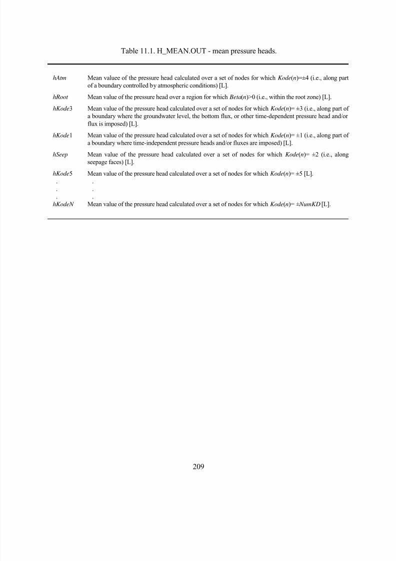
8/20/2019 HYDRUS3D Technical Manual.pdf
http://slidepdf.com/reader/full/hydrus3d-technical-manualpdf 239/260
209
Table 11.1. H_MEAN.OUT - mean pressure heads.
hAtm Mean valuee of the pressure head calculated over a set of nodes for which Kode(n)=±4 (i.e., along partof a boundary controlled by atmospheric conditions) [L].
hRoot Mean value of the pressure head over a region for which Beta(n)>0 (i.e., within the root zone) [L].hKode3 Mean value of the pressure head calculated over a set of nodes for which Kode(n)= ±3 (i.e., along part of
a boundary where the groundwater level, the bottom flux, or other time-dependent pressure head and/orflux is imposed) [L].
hKode1 Mean value of the pressure head calculated over a set of nodes for which Kode(n)= ±1 (i.e., along part ofa boundary where time-independent pressure heads and/or fluxes are imposed) [L].
hSeep Mean value of the pressure head calculated over a set of nodes for which Kode(n)= ±2 (i.e., alongseepage faces) [L].
hKode5 Mean value of the pressure head calculated over a set of nodes for which Kode(n)= ±5 [L].. .. .
. .hKodeN Mean value of the pressure head calculated over a set of nodes for which Kode(n)= ± NumKD [L].
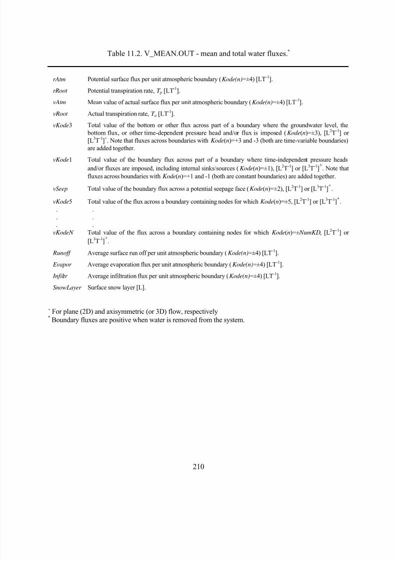
8/20/2019 HYDRUS3D Technical Manual.pdf
http://slidepdf.com/reader/full/hydrus3d-technical-manualpdf 240/260
210
Table 11.2. V_MEAN.OUT - mean and total water fluxes.*
rAtm Potential surface flux per unit atmospheric boundary (Kode(n)=±4) [LT-1].
rRoot Potential transpiration rate, T p [LT-1].
vAtm Mean value of actual surface flux per unit atmospheric boundary (Kode(n)=±4) [LT-1].
vRoot Actual transpiration rate, T a [LT-1].
vKode3 Total value of the bottom or other flux across part of a boundary where the groundwater level, the bottom flux, or other time-dependent pressure head and/or flux is imposed (Kode(n)=±3), [L2T-1] or[L3T-1]+. Note that fluxes across boundaries with Kode(n)=+3 and -3 (both are time-variable boundaries)are added together.
vKode1 Total value of the boundary flux across part of a boundary where time-independent pressure headsand/or fluxes are imposed, including internal sinks/sources (Kode(n)=±1), [L2T-1] or [L3T-1]+. Note thatfluxes across boundaries with Kode(n)=+1 and -1 (both are constant boundaries) are added together.
vSeep Total value of the boundary flux across a potential seepage face (Kode(n)=±2), [L2T-1] or [L3T-1]+.
vKode5 Total value of the flux across a boundary containing nodes for which Kode(n)=±5, [L2T-1] or [L3T-1]+.. .. .. .
vKodeN Total value of the flux across a boundary containing nodes for which Kode(n)=± NumKD, [L2T-1] or[L3T-1]+.
Runoff Average surface run off per unit atmospheric boundary (Kode(n)=±4) [LT-1].
Evapor Average evaporation flux per unit atmospheric boundary (Kode(n)=±4) [LT-1].
Infiltr Average infiltration flux per unit atmospheric boundary (Kode(n)=±4) [LT-1].
SnowLayer Surface snow layer [L].
+ For plane (2D) and axisymmetric (or 3D) flow, respectively* Boundary fluxes are positive when water is removed from the system.
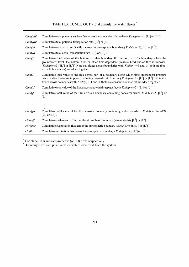
8/20/2019 HYDRUS3D Technical Manual.pdf
http://slidepdf.com/reader/full/hydrus3d-technical-manualpdf 241/260
211
Table 11.3. CUM_Q.OUT - total cumulative water fluxes.*
CumQAP Cumulative total potential surface flux across the atmospheric boundary (Kode(n)=±4), [L2] or [L3]+.
CumQRP Cumulative total potential transpiration rate, [L2] or [L3]+.
CumQA Cumulative total actual surface flux across the atmospheric boundary (Kode(n)=±4), [L2] or [L3]+.
CumQR Cumulative total actual transpiration rate, [L2] or [L3]+.
CumQ3 Cumulative total value of the bottom or other boundary flux across part of a boundary where thegroundwater level, the bottom flux, or other time-dependent pressure head and/or flux is imposed(Kode(n)=±3), [L2] or [L3]+. Note that fluxes across boundaries with Kode(n)=+3 and -3 (both are time-variable boundaries) are added together.
CumQ1 Cumulative total value of the flux across part of a boundary along which time-independent pressureheads and/or fluxes are imposed, including internal sinks/sources (Kode(n)=±1), [L2] or [L3]+. Note thatfluxes across boundaries with Kode(n)=+1 and -1 (both are constant boundaries) are added together.
CumQS Cumulative total value of the flux across a potential seepage faces (Kode(n)=±2), [L2] or [L3]+.
CumQ5 Cumulative total value of the flux across a boundary containing nodes for which Kode(n)=±5, [L2
] or[L3]+.. .. .. .
CumQN Cumulative total value of the flux across a boundary containing nodes for which Kode(n)=± NumKD,[L2] or [L3]+.
cRunoff Cumulative surface run off across the atmospheric boundary (Kode(n)=±4), [L2] or [L3]+.
cEvapor Cumulative evaporation flux across the atmospheric boundary (Kode(n)=±4), [L2] or [L3]+.
c Infiltr Cumulative infiltration flux across the atmospheric boundary (Kode(n)=±4), [L2] or [L3]+.
+ For plane (2D) and axisymmetric (or 3D) flow, respectively* Boundary fluxes are positive when water is removed from the system.
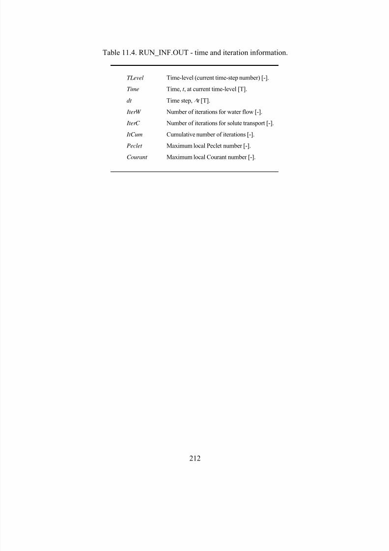
8/20/2019 HYDRUS3D Technical Manual.pdf
http://slidepdf.com/reader/full/hydrus3d-technical-manualpdf 242/260
212
Table 11.4. RUN_INF.OUT - time and iteration information.
TLevel Time-level (current time-step number) [-].
Time Time, t , at current time-level [T].
dt Time step, ∆t [T].
IterW Number of iterations for water flow [-].
IterC Number of iterations for solute transport [-].
ItCum Cumulative number of iterations [-].
Peclet Maximum local Peclet number [-].
Courant Maximum local Courant number [-].
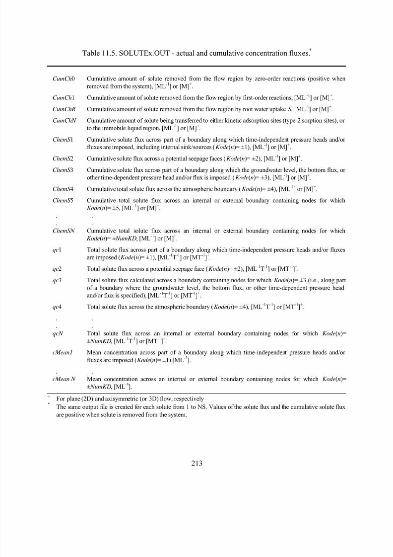
8/20/2019 HYDRUS3D Technical Manual.pdf
http://slidepdf.com/reader/full/hydrus3d-technical-manualpdf 243/260
213
Table 11.5. SOLUTEx.OUT - actual and cumulative concentration fluxes.*
CumCh0 Cumulative amount of solute removed from the flow region by zero-order reactions (positive whenremoved from the system), [ML-1] or [M]+.
CumCh1 Cumulative amount of solute removed from the flow region by first-order reactions, [ML-1] or [M]+.CumChR Cumulative amount of solute removed from the flow region by root water uptake S , [ML-1] or [M]+.
CumChN Cumulative amount of solute being transferred to either kinetic adsorption sites (type-2 sorption sites), orto the immobile liquid region, [ML-1] or [M]+.
ChemS 1 Cumulative solute flux across part of a boundary along which time-independent pressure heads and/orfluxes are imposed, including internal sink/sources (Kode(n)= ±1), [ML-1] or [M]+.
ChemS 2 Cumulative solute flux across a potential seepage faces (Kode(n)= ±2), [ML-1] or [M]+.
ChemS 3 Cumulative solute flux across part of a boundary along which the groundwater level, the bottom flux, orother time-dependent pressure head and/or flux is imposed (Kode(n)= ±3), [ML-1] or [M]+.
ChemS 4 Cumulative total solute flux across the atmospheric boundary (Kode(n)= ±4), [ML-1] or [M]+.
ChemS 5 Cumulative total solute flux across an internal or external boundary containing nodes for whichKode(n)= ±5, [ML-1] or [M]+.
. .
. .ChemSN Cumulative total solute flux across an internal or external boundary containing nodes for which
Kode(n)= ± NumKD, [ML-1] or [M]+.
qc1 Total solute flux across part of a boundary along which time-independent pressure heads and/or fluxesare imposed (Kode(n)= ±1), [ML-1T-1] or [MT-1]+.
qc2 Total solute flux across a potential seepage face (Kode(n)= ±2), [ML-1T-1] or [MT-1]+.
qc3 Total solute flux calculated across a boundary containing nodes for which Kode(n)= ±3 (i.e., along partof a boundary where the groundwater level, the bottom flux, or other time-dependent pressure headand/or flux is specified), [ML-1T-1] or [MT-1]+.
qc4 Total solute flux across the atmospheric boundary (Kode(n)= ±4), [ML-1T-1] or [MT-1]+.
. .
. .qcN Total solute flux across an internal or external boundary containing nodes for which Kode(n)=
± NumKD, [ML-1T-1] or [MT-1]+.
cMean1 Mean concentration across part of a boundary along which time-independent pressure heads and/orfluxes are imposed (Kode(n)= ±1) [ML-3].
. .cMean N Mean concentration across an internal or external boundary containing nodes for which Kode(n)=
± NumKD, [ML-3].
+ For plane (2D) and axisymmetric (or 3D) flow, respectively* The same output file is created for each solute from 1 to NS. Values of the solute flux and the cumulative solute flux
are positive when solute is removed from the system.
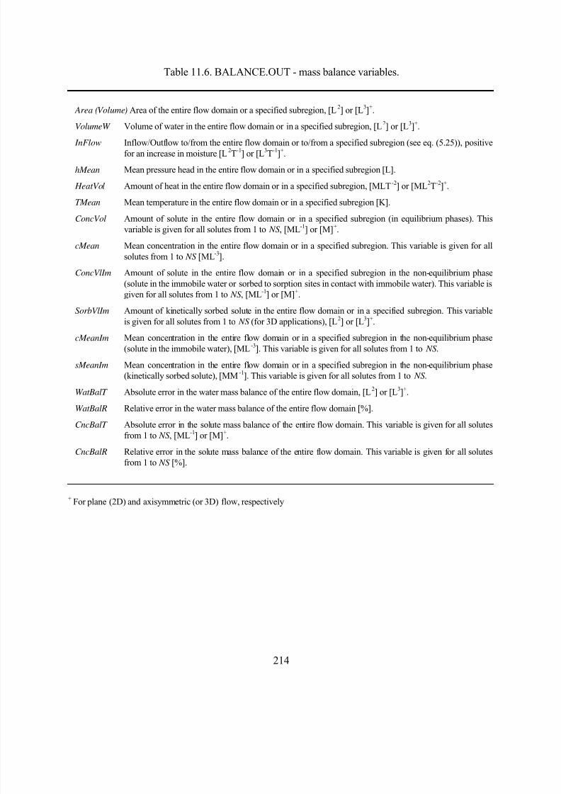
8/20/2019 HYDRUS3D Technical Manual.pdf
http://slidepdf.com/reader/full/hydrus3d-technical-manualpdf 244/260
214
Table 11.6. BALANCE.OUT - mass balance variables.
Area (Volume) Area of the entire flow domain or a specified subregion, [L2] or [L3]+.
VolumeW Volume of water in the entire flow domain or in a specified subregion, [L2] or [L3]+.
InFlow Inflow/Outflow to/from the entire flow domain or to/from a specified subregion (see eq. (5.25)), positivefor an increase in moisture [L2T-1] or [L3T-1]+.
hMean Mean pressure head in the entire flow domain or in a specified subregion [L].
HeatVol Amount of heat in the entire flow domain or in a specified subregion, [MLT-2] or [ML2T-2]+.
TMean Mean temperature in the entire flow domain or in a specified subregion [K].
ConcVol Amount of solute in the entire flow domain or in a specified subregion (in equilibrium phases). Thisvariable is given for all solutes from 1 to NS , [ML-1] or [M]+.
cMean Mean concentration in the entire flow domain or in a specified subregion. This variable is given for allsolutes from 1 to NS [ML-3].
ConcVlIm Amount of solute in the entire flow domain or in a specified subregion in the non-equilibrium phase(solute in the immobile water or sorbed to sorption sites in contact with immobile water). This variable isgiven for all solutes from 1 to NS , [ML-1] or [M]+.
SorbVlIm Amount of kinetically sorbed solute in the entire flow domain or in a specified subregion. This variableis given for all solutes from 1 to NS (for 3D applications), [L2] or [L3]+.
cMeanIm Mean concentration in the entire flow domain or in a specified subregion in the non-equilibrium phase(solute in the immobile water), [ML-3]. This variable is given for all solutes from 1 to NS .
sMeanIm Mean concentration in the entire flow domain or in a specified subregion in the non-equilibrium phase(kinetically sorbed solute), [MM-1]. This variable is given for all solutes from 1 to NS .
WatBalT Absolute error in the water mass balance of the entire flow domain, [L2] or [L3]+.
WatBalR Relative error in the water mass balance of the entire flow domain [%].
CncBalT Absolute error in the solute mass balance of the entire flow domain. This variable is given for all solutesfrom 1 to NS , [ML-1] or [M]+.
CncBalR Relative error in the solute mass balance of the entire flow domain. This variable is given for all solutesfrom 1 to NS [%].
+ For plane (2D) and axisymmetric (or 3D) flow, respectively
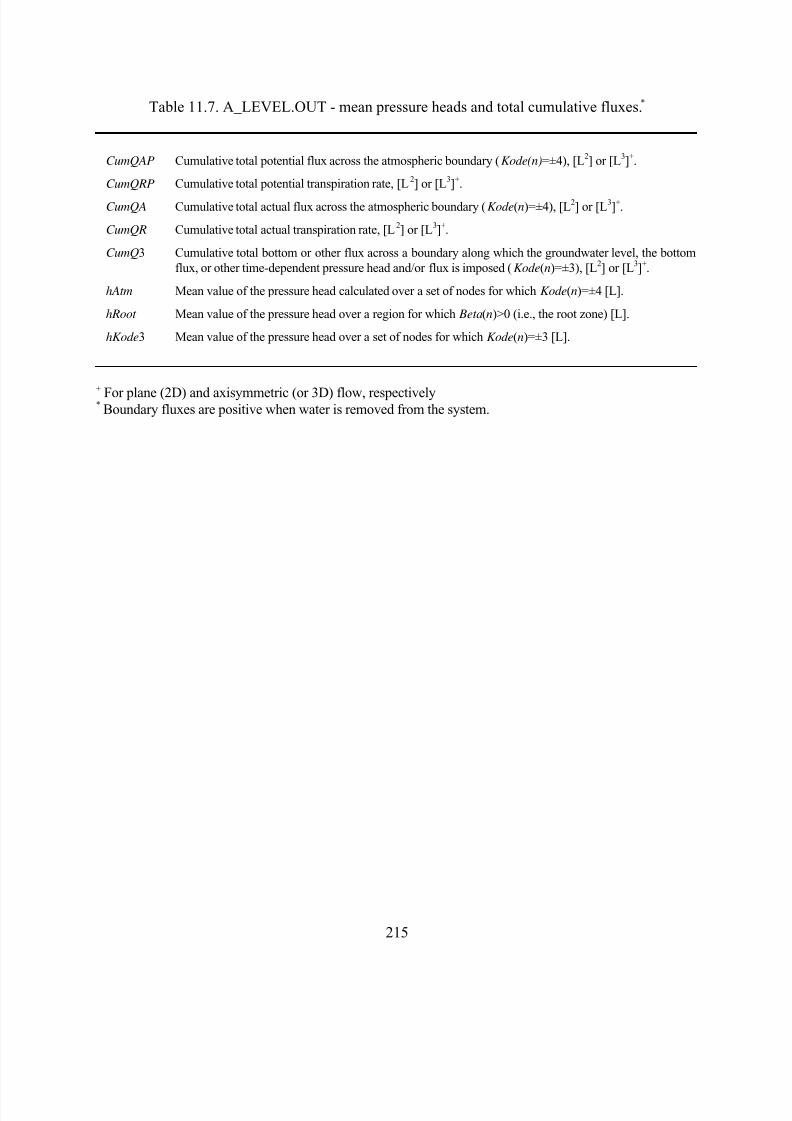
8/20/2019 HYDRUS3D Technical Manual.pdf
http://slidepdf.com/reader/full/hydrus3d-technical-manualpdf 245/260
215
Table 11.7. A_LEVEL.OUT - mean pressure heads and total cumulative fluxes.*
CumQAP Cumulative total potential flux across the atmospheric boundary (Kode(n)=±4), [L2] or [L3]+.
CumQRP Cumulative total potential transpiration rate, [L2] or [L3]+.
CumQA Cumulative total actual flux across the atmospheric boundary (Kode(n)=±4), [L2] or [L3]+.
CumQR Cumulative total actual transpiration rate, [L2] or [L3]+.
CumQ3 Cumulative total bottom or other flux across a boundary along which the groundwater level, the bottomflux, or other time-dependent pressure head and/or flux is imposed (Kode(n)=±3), [L2] or [L3]+.
hAtm Mean value of the pressure head calculated over a set of nodes for which Kode(n)=±4 [L].
hRoot Mean value of the pressure head over a region for which Beta(n)>0 (i.e., the root zone) [L].
hKode3 Mean value of the pressure head over a set of nodes for which Kode(n)=±3 [L].
+ For plane (2D) and axisymmetric (or 3D) flow, respectively* Boundary fluxes are positive when water is removed from the system.
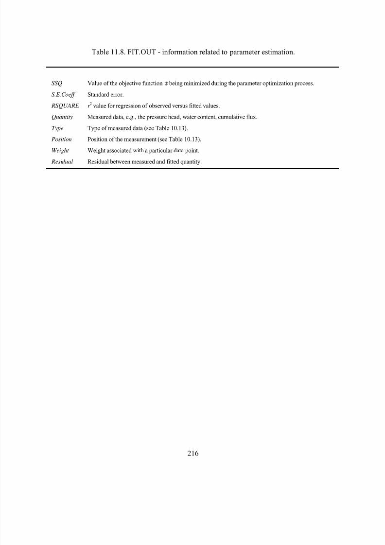
8/20/2019 HYDRUS3D Technical Manual.pdf
http://slidepdf.com/reader/full/hydrus3d-technical-manualpdf 246/260
216
Table 11.8. FIT.OUT - information related to parameter estimation.
SSQ Value of the objective functionΦ being minimized during the parameter optimization process.
S.E.Coeff Standard error. RSQUARE r 2 value for regression of observed versus fitted values.
Quantity Measured data, e.g., the pressure head, water content, cumulative flux.
Type Type of measured data (see Table 10.13).
Position Position of the measurement (see Table 10.13).
Weight Weight associated with a particular data point.
Residual Residual between measured and fitted quantity.
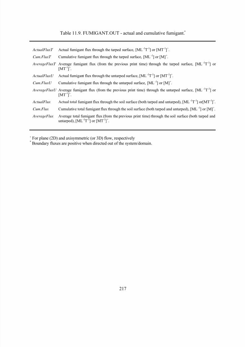
8/20/2019 HYDRUS3D Technical Manual.pdf
http://slidepdf.com/reader/full/hydrus3d-technical-manualpdf 247/260
217
Table 11.9. FUMIGANT.OUT - actual and cumulative fumigant.*
ActualFluxT Actual fumigant flux through the tarped surface, [ML-1T-1] or [MT-1]+.
Cum.FluxT Cumulative fumigant flux through the tarped surface, [ML-1] or [M]+.
AverageFluxT Average fumigant flux (from the previous print time) through the tarped surface, [ML-1T-1] or[MT-1]+.
ActualFluxU Actual fumigant flux through the untarped surface, [ML-1T-1] or [MT-1]+.
Cum.FluxU Cumulative fumigant flux through the untarped surface, [ML-1] or [M]+.
AverageFluxU Average fumigant flux (from the previous print time) through the untarped surface, [ML -1T-1] or[MT-1]+.
ActualFlux Actual total fumigant flux through the soil surface (both tarped and untarped), [ML-1T-1] or[MT-1]+.
Cum.Flux Cumulative total fumigant flux through the soil surface (both tarped and untarped), [ML-1] or [M]+.
AverageFlux Average total fumigant flux (from the previous print time) through the soil surface (both tarped and
untarped), [ML-1
T-1
] or [MT-1
]+
.
+ For plane (2D) and axisymmetric (or 3D) flow, respectively* Boundary fluxes are positive when directed out of the system/domain.

8/20/2019 HYDRUS3D Technical Manual.pdf
http://slidepdf.com/reader/full/hydrus3d-technical-manualpdf 248/260
218
8/20/2019 HYDRUS3D Technical Manual.pdf
http://slidepdf.com/reader/full/hydrus3d-technical-manualpdf 249/260
219
12. REFERENCES
Adamczyk, Z., B. Siwek, M Zembala, and P. Belouschek, Kinetics of localized adsorption ofcolloid particles, Adv. Colloid Interface Sci., 48 , 151-280, 1994.
Alexander, M., and K. M. Scow, Kinetics of biodegradation in soil, In Reactions and Movement of
Organic Chemicals in Soils, edited by B. L. Sawhney and K. Brown, Spec. Publ. No. 22, 243-270, Soil Science Society of America, Madison, WI, 1989.
Bar-Yosef, B., Advances in fertigation, Advances in Agronomy, 65, 1-77, 1999.
Bear, J., Dynamics of Fluid in Porous Media. Elsevier, New York, NY, 1972.
Behie, A., and P. Forsyth, Jr., Comparison of fast iterative methods for symmetric systems. IMA J.of Numerical Analysis, 3, 41-63, 1983.
Belmans, C., J. G. Wesseling and R. A. Feddes, Simulation model of the water balance of acropped soil: SWATRE, J. Hydrol., 63, 271- 286, 1983.
Bradford, S. A., S. R. Yates, M. Bettahar, and J. Šimůnek, Physical factors affecting the transportand fate of colloids in saturated porous media, Water Resour. Res. 38(12), 1327,doi:10.1029/2002WR001340, 2002.
Bradford, S. A., J. Šimůnek, M. Bettahar, M. Th. van Genuchten, and S. R . Yates, Modeling colloidattachment, straining, and exclusion in saturated porous media, Environ. Sci. Technol., 37 ,2242-2250, 2003.
Bradford, S. A., M. Bettahar, J. Šimůnek, and M. Th. Van Genuchten, Straining and attachment ofcolloids in physically heterogeneous porous media, Vadose Zone J., 3, 384-394, 2004.
Bromilow, R. H., and M. Leistra, Measured and simulated behavior of aldicarb and its oxidation products in fallow soils, Pestic. Sci., 11(4), 389-395, 1980.
Brooks, R. H., and A. T. Corey, Hydraulic properties of porous media, Hydrol. Paper No. 3,Colorado State Univ., Fort Collins, CO, 1964.
Castro, C. L., and D. E. Rolston, Organic phosphate transport and hydrolysis in soil: theoretical andexperimental evaluation, Soil Sci. Soc. Am. J., 41(6), 1085-1092, 1977.
Celia, M. A., and E. T. Bououtas, R. L. Zarba, A general mass-conservative numerical solution forthe unsaturated flow equation, Water Resour. Res., 26 , 1483-1496, 1990.
Chiou, C. T., Theoretical consideration of the partition uptake of nonionic organic compounds bysoil organic matter, In Reactions and Movement of Organic Chemicals in Soils, edited by B. L.Sawhney and K. Brown, Spec. Publ. Number 22, 1-30, Soil Science Society of America,Madison, WI, 1989.
Chung S.-O., and R. Horton, Soil heat and water flow with a partial surface mulch, Water Resour. Res., 23(12), 2175-2186, 1987.
Cho, C. M., Convective transport of ammonium with nitrification in soil, Can. Jour. Soil Sci.,
8/20/2019 HYDRUS3D Technical Manual.pdf
http://slidepdf.com/reader/full/hydrus3d-technical-manualpdf 250/260
220
51(3), 339-350, 1971.
Christie, L. D., D. F. Griffiths, A. R. Mitchell, and O. C. Zienkiewicz, Finite element methods forsecond order differential equations with significant first derivatives, Int. J. Num. Methods inEngineering, 10, 1389-1396, 1976.
Císlerová, M., Comparison of simulated water balance for ordinary and scaled soil hydrauliccharacteristics, Publ. No. 82, Dept. of Hydraulics and Catchment Hydrology, AgriculturalUniv., Wageningen, The Netherlands, 1987.
Cleary, R. W., and M. J. Ungs, Groundwater pollution and hydrology, Mathematical models andcomputer programs, Research Rep. No. 78-WR-15, Water Resour. Program, Princeton Univ.Princeton, NJ, 1978.
Clausnitzer, V., and J. W. Hopmans, Non-linear parameter estimation: LM_OPT. General-purposeoptimization code based on the Levenberg-Marquardt algorithm, Land, Air and Water Resources Paper No. 100032, University of California, Davis, CA, 1995.
Constantz, J., Temperature dependence of unsaturated hydraulic conductivity of two soils. Soil Sci.
Soc. Am. J., 46 (3), 466-470, 1982.Daniel, C., and F. S. Wood, Fitting Equations to Data. Wiley-Interscience, New York, 1971.
Davis, L. A., and S. P. Neuman, Documentation and user's guide: UNSAT2 - Variably saturatedflow model, Final Rep., WWL/TM-1791-1, Water, Waste & Land, Inc., Ft. Collins, CO, 1983.
de Marsily, G., Quantitative Hydrogeology, Academic Press, London, 1986.
de Vries, D. A., The thermal properties of soils, In Physics of Plant Environment , edited by R. W.van Wijk, pp. 210-235, North Holland, Amsterdam, 1963.
Durner, W., Hydraulic conductivity estimation for soils with heterogeneous pore structure, Water Resour. Res., 32(9), 211-223, 1994.
Durner, W., E. Priesack, H.-J. Vogel, and T. Zurmühl, Determination of parameters for flexiblehydraulic functions by inverse modeling. In: M.Th. van Genuchten, F.J. Leij, L. Wu (Editors),Characterization and Measurement of the Hydraulic Properties of Unsaturated Porous Media.University of California, Riverside, CA, pp. 817-829, 1999.
Edwards, W. M., R. R. van der Ploeg, and W. Ehlers, A numerical study of the effects ofnoncapillary-sized pores upon infiltration, Soil Sci. Soc. Am. J., 43, 851-856, 1979.
Feddes, R. A., E. Bresler, and S. P. Neuman, Field test of a modified numerical model for wateruptake by root systems, Water Resour. Res., 10(6), 1199-1206, 1974.
Feddes, R. A., P. J. Kowalik, and H. Zaradny, Simulation of Field Water Use and Crop Yield , John
Wiley & Sons, New York, NY, 1978.Fipps, G., R. W. Skaggs, and J. L. Nieber, Drains as a boundary condition in finite elements, Water
Resour. Res., 22(11), 1613-1621, 1986.
Flint, A. L., L. E. Flint, G. S. Bodvarsson, E. M. Kwicklis, and J. Fabryka-Martin, Development of
8/20/2019 HYDRUS3D Technical Manual.pdf
http://slidepdf.com/reader/full/hydrus3d-technical-manualpdf 251/260
221
the conceptual model of unsaturated zone hydrology at Yucca Mountain, Nevada, In:Conceptual Models of Flow and Transport in the Fractured Vadose zone, National ResearchCouncil, National Academy Press, Washington, D.C., pp. 47-85, 2001.
Gärdenäs, A., Hopmans, J. W., B. R. Hanson, and J. Šimůnek, Two-dimensional modeling ofnitrate leaching for various fertigation scenarios under micro-irrigation, Agric. Water
Management, 74, 219-242, 2005.Gerke, H. H., and M. Th. van Genuchten, A dual-porosity model for simulating the preferential
movement of water and solutes in structured porous media, Water Resour. Res., 29, 305-319,1993a.
Gerke, H. H., and M. Th. van Genuchten, Evaluation of a first-order water transfer term for variablysaturated dual-porosity flow models, Water Resour. Res., 29, 1225-1238, 1993b.
Gerke, H. H., and M. Th. van Genuchten, Macroscopic representation of structural geometry forsimulating water and solute movement in dual-porosity media, Adv. Water Resour., 19, 343-357, 1996.
Germann, P. F., Kinematic wave approach to infiltration and drainage into and from soilmacropores, Trans. ASAE , 28 , 745-749, 1985.
Germann, P. F., and G. Beven, Kinematic wave approximation to infiltration into soils with sorbingmacropores, Water Resour. Res., 21(7), 990-996, 1985.
Glotfelty, D. E., and C. J. Schomburg, Volatilization of pesticides from soil, In Reactions and Movement of Organic Chemicals in Soils, edited by B. L. Sawhney and K. Brown, Spec. Publ. Number 22, 181-208, Soil Science Society of America, Madison, WI, 1989.
Gribb, M. M., Parameter estimation for determining hydraulic properties of a fine sand fromtransient flow measurements, Water Resour. Res., 32(7), 1965-1974, 1996.
Gribb, M. M., J. Šimůnek, and M. F. Leonard, Development of a cone penetrometer method todetermine soil hydraulic properties, ASCE J. of Geotech. and Geoenviron. Eng., 124(9), 820-829, 1998.
Gureghian, A. B., A two-dimensional finite-element solution for the simultaneous transport ofwater and multi-solutes through a nonhomogeneous aquifer under transient saturated-unsaturated flow conditions, Sci. Total Environ., 21, 329-337, 1981.
Gureghian, A. B., and G. Jansen, LAYFLO: A one-dimensional semianalytical model for themigration of a three-member decay chain in a multilayered geologic medium, Tech. Rep.ONWI-466 , Office of Nuclear Waste Isolation, Battelle Memorial Institute, Columbus, OH,1983.
Harada, M., P. L. Chambre, M. Foglia, K. Higashi, F. Iwamoto, D. Leung, T. H. Pigford, and D.Ting, Migration of radionuclides through sorbing media, analytical solutions - I, Rep. no. LBL-10500 (UC-11), Lawrence Berkeley Laboratory, Univ. of California, Berkeley, CA, 1980.
Higashi, K., and T. H. Pigford, Analytical models for migration of radionuclides in geologic
8/20/2019 HYDRUS3D Technical Manual.pdf
http://slidepdf.com/reader/full/hydrus3d-technical-manualpdf 252/260
222
sorbing media, J. Nucl. Sci. and Techn., 7 (9), 700-709, 1980.
Hopmans, J. W., and J. N. M. Stricker, Stochastic analysis of soil water regime in a watershed, J. Hydrol., 105, 57-84, 1989.
Huyakorn, P. S., and G. F. Pinder, Computational Methods in Subsurface Flow, Academic Press,
London, United Kingdom, 1983.Inoue, M., J. Šimůnek, J. W. Hopmans, and V. Clausnitzer, In-situ estimation of soil hydraulic
functions using a multi-step soil water extraction technique, Water Resour. Rer., 34(5), 1035-1050, 1998.
Javandel, I., Ch. Doughty, Chin-Fu Tsang, Groundwater Transport: Handbook of Mathematical Models, Water Resour. Monograph No. 10, Am. Geophys. Union, Washington, D.C., 1984.
Johnson, P. R., and M. Elimelech, Dynamics of colloid deposition in porous media: Blocking basedon random sequential adsorption, Langmuir , 11, 801-812, 1995.
Jungk, A. O., Dynamics of nutrient movement at the soil-root interface, Chapter 31 in: Y. Waisel,A. Eshel, and U. Kafkafi, Eds., Plant Roots, The Hidden Half, Marcel Dekker, Inc. New York,455-481, 1991.
Jury, W. A., W. F. Spencer, and W. J. Farmer, Behavior assessment model for trace organics insoil, I. Model description, J. Environ. Qual., 12, 558-564, 1983.
Köhne, J. M., S. Köhne, B. P. Mohanty, and J. Šimůnek, Inverse mobile-immobile modeling oftransport during transient flow: Effect of between-domain transfer and initial water content,Vadose Zone Journal, 3(4), 1309-1321, 2004.
Köhne, S., B. Lennartz, J. M. Köhne, and J. Šimůnek, Bromide transport at a tile-drained field site:experiment, one- and two-dimensional equilibrium and non-equilibrium numerical modeling, J. Hydrology, 321(1-4), 390-408, 2006.
Kirkham, D., Flow of ponded water into drain tubes in soil overlying an impervious layer, Trans. Amer. Geoph. Union, 30(3), 369-385, 1949.
Kirkham, D., and W. L. Powers, Advanced Soil Physics, John Wiley & Sons, New York, NY, 1972.
Kodešová, R., M. M. Gribb, and J. Šimůnek, Estimating soil hydraulic properties from transientcone permeameter data, Soil Science, 163(6), 436-453, 1998.
Kool, J. B., J. C. Parker, and M. Th. van Genuchten, Determining soil hydraulic properties fromone-step outflow experiments by parameter estimation: I. Theory and numerical studies, SoilSci. Soc. Am. J., 49, 1348-1354, 1985.
Kool, J. B., and J. C. Parker, Development and evaluation of closed-form expressions for hysteretic
soil hydraulic properties. Water Resour. Res., 23(1), 105-114, 1987.Kool, J. B., J. C. Parker, and M. Th. van Genuchten, Parameter estimation for unsaturated flow and
transport models - A review, J. Hydrol., 91, 255-293, 1987.
Kool, J. B., M. Th. van Genuchten, HYDRUS - One-dimensional variably saturated flow and
8/20/2019 HYDRUS3D Technical Manual.pdf
http://slidepdf.com/reader/full/hydrus3d-technical-manualpdf 253/260
223
transport model, including hysteresis and root water uptake, Version 3.3, Research Report No.124, U. S. Salinity Laboratory, USDA, ARS, Riverside, CA, 1991.
Kosugi K., Lognormal distribution model for unsaturated soil hydraulic properties, Water Resour. Res., 32(9), 2697-2703, 1996.
Langergraber, G. and J. Šimůnek, Modeling variably-saturated water flow and multi-componentreactive transport in constructed wetlands, Vadose Zone Journal, 4, 924-938, 2005.
Langergraber, G., and J. Šimůnek, The Multi-component Reactive Transport Module CW2D forConstructed Wetlands for the HYDRUS Software Package, Manual – Version 1.0, HYDRUSSoftware Series 2, Department of Environmental Sciences, University of California Riverside,Riverside, CA, 72 pp., 2006.
Lazarovitch, N., J. Šimůnek, and U. Shani, System dependent boundary condition for water flowfrom subsurface source, Soil Sci. Soc. Am. J., 69(1), 46-50, 2005.
Leij, F. J., T. H. Skaggs, and M. Th. van Genuchten, Analytical solutions for solute transport inthree-dimensional semi-infinite porous media, Water Resour. Res., 27 (10), 2719-2733, 1991.
Leij, F. J., and S. A. Bradford, 3DADE: A computer program for evaluating three-dimensionalequilibrium solute transport in porous media, Research Report No. 134, U. S. SalinityLaboratory, USDA, ARS, Riverside, CA, 1994.
Logan, B. E., D. G. Jewett, R. G. Arnold, E. J. Bouwer, and C. R. O’Melia, Clarification of clean- bed filtration models, J. Environ. Eng., 121, 869-873, 1995.
Lenhard, R. J., J. C. Parker, and J. J. Kaluarachchi, Comparing simulated and experimentalhysteretic two-phase transient fluid flow phenomena, Water Resour. Res., 27 (8), 2113-2124,1991.
Lenhard, R. J., and J. C. Parker, Modeling multiphase fluid hysteresis and comparing results to
laboratory investigations, In, Proc. Intl. Workshop on Indirect Methods for Estimating the Hydraulic Properties of Unsaturated Soils, edited by M. Th van Genuchten, F. J. Leij, and L. J.Lund, University of California, Riverside, pp. 233-248,1992.
Lester, D. H., G. Jansen, and H. C. Burkholder, Migration of radionuclide chains through anadsorbing medium, In: Adsorption and Ion Exchange, Am. Inst. Chem. Eng., Symp. Series no.152, 71, 202-213, 1975.
Letniowski, F. W., An overview of preconditioned iterative methods for sparse matrix equations. Research Report CS-89-26, Faculty of Mathematics, Univ. of Waterloo, Waterloo, Ontario,Canada, 1989.
Luckner, L., M. Th. van Genuchten, and D. R. Nielsen, A consistent set of parametric models for
the two-phase flow of immiscible fluids in the subsurface. Water Resour. Res., 25(10), 2187-2193, 1989.
Lynch, D., Mass conservation in finite element groundwater models. Adv. Water Resour., 7 , 67-75,1984.
8/20/2019 HYDRUS3D Technical Manual.pdf
http://slidepdf.com/reader/full/hydrus3d-technical-manualpdf 254/260
8/20/2019 HYDRUS3D Technical Manual.pdf
http://slidepdf.com/reader/full/hydrus3d-technical-manualpdf 255/260
225
Finite Elements in Fluids, Vol. I, Viscous Flow and Hydrodynamics, edited by R. H. Gallagher,J. T. Oden, C. Taylor, and O.C. Zienkiewicz, John Wiley & Sons, London, pp. 201-217, 1975.
Nielsen, D. R., and L. M. Luckner, Theoretical aspects to estimate reasonable initial parameters andrange limits in indentification procedures for soil hydraulic properties. In, Proc. Intl. Workshopon Indirect Methods for Estimating the Hydraulic Properties of Unsaturated Soils, edited by M.
Th van Genuchten, F. J. Leij, and L. J. Lund, University of California, Riverside, pp. 147-160,1992.
Ou, L. T., P. S. C. Rao, K. S. V. Edvardson, R. E. Jessup, A. G. Hornsby, and R. L. Jones, Aldicarbdegradation in sandy soils from different depths, Pesticide Sci., 23, 1-12, 1988.
Perrochet, P., and D. Berod, Stability of the standard Crank-Nicolson-Galerkin scheme applied tothe diffusion-convection equation: some new insights, Water Resour. Res., 29(9), 3291-3297,1993.
Peters, R. R., and E. A. Klavetter, A continuum model for water movement in an unsaturatedfractured rock mass, Water Resour. Res., 24(3), 416-430, 1988.
Philip, J. R., and D. A. de Vries, Moisture movement in porous media under temperature gradients,Eos Trans. AGU, 38 (2), 222-232, 1957.
Phillip, J. R., The theory of absorption in aggregated media, Aust. J. Soil Res., 6 , 1-19, 1968.
Pignatello, J. J., Sorption dynamics of organic compounds in soils and sediments, In Reactions and Movement of Organic Chemicals in Soils, edited by B. L. Sawhney and K. Brown, Spec. Publ. Number 22, 45-80, Soil Science Society of America, Madison, WI, 1989.
Pinder, G. F., W. G. Gray, Finite Element Simulation in Surface and Subsurface Hydrology,Academic Press, New York, N.Y., 1977.
Pruess, K., and J. S. Y. Wang, Numerical modeling of isothermal and non-isothermal flow in
unsaturated fractured rock - a review, In: D. D. Evans, and T. J. Nicholson (Editors), Flow andTransport Through Unsaturated Fractured Rock, Geophysics Monograph 42, AmericanGeophysical Union, Washington, D.C., pp. 11-22, 1987.
Rajagopalan, R., and C. Tien, Trajectory analysis of deep-bed filtration with the sphere-in-cell porous media model, AIChE. J ., 22, 523-533, 1976.
Rogers, V. C., Migration of radionuclide chains in groundwater, Nucl. Techn., 40(3), 315-320,1978.
Rogers, J. S., and J. L. Fouss, Hydraulic conductivity determination from vertical and horizontaldrains in layered soil profiles, Transaction of the ASAE, 32(2), 589-595, 1989.
Schijven, J., and J. Šimůnek, Kinetic modeling of virus transport at field scale, J. of Contam. Hydrology, 55(1-2), 113-135, 2002.
Scott, P. S., G. J. Farquhar, and N. Kouwen, Hysteresis effects on net infiltration, Advances inInfiltration, Publ. 11-83, pp.163-170, Am. Soc. Agri. Eng., St. Joseph, Mich., 1983.
8/20/2019 HYDRUS3D Technical Manual.pdf
http://slidepdf.com/reader/full/hydrus3d-technical-manualpdf 256/260
226
Šejna, M., J. Šimůnek, and M. Th. van Genuchten, The HYDRUS Software Package for SimulatingTwo- and Three-Dimensional Movement of Water, Heat, and Multiple Solutes in Variably-Saturated Porous Media, User Manual, Version 1.0, PC Progress, Prague, Czech Republic,2011.
Selim, H. M., R. Schulin, and H. Flühler, Transport and ion exchange of calcium and magnesium in
an aggregated soil, Soil Sci. Soc. Am. J., 51(4), 876-884, 1987.Simmons, C. S., D. R. Nielsen, and J. W. Biggar, Scaling of field-measured soil water properties,
Hilgardia, 47 , 101-122, 1980.
Šimůnek, J., T. Vogel and M. Th. van Genuchten, The SWMS_2D code for simulating water flowand solute transport in two-dimensional variably saturated media, Version 1.1, Research Report No. 126 , U. S. Salinity Laboratory, USDA, ARS, Riverside, CA, 1992.
Šimůnek, J., and D. L. Suarez, Modeling of carbon dioxide transport and production in soil: 1.Model development, Water Resour. Res., 29(2), 487-497, 1993a.
Šimůnek, J., and D. L. Suarez, UNSATCHEM-2D code for simulating two-dimensional variably
saturated water flow, heat transport, carbon dioxide production and transport, andmulticomponent solute transport with major ion equilibrium and kinetic chemistry, Version 1.1, Research Report No. 128 , U. S. Salinity Laboratory, USDA, ARS, Riverside, CA, 1993b.
Šimůnek, J., and D. L. Suarez, Two-dimensional transport model for variably saturated porousmedia with major ion chemistry, Water Resour. Res., 30(4), 1115-1133, 1994.
Šimůnek, J., and M. Th. van Genuchten, The CHAIN_2D code for the two-dimensional movementof water, heat, and multiple solutes in variably saturated media, Version 1.1, Research Report No. 136 , U. S. Salinity Laboratory, USDA, ARS, Riverside, CA, 1994.
Šimůnek, J., T. Vogel and M. Th. van Genuchten, The SWMS_2D code for simulating water flowand solute transport in two-dimensional variably saturated media, Version 1.1, Research Report
No. 132, U. S. Salinity Laboratory, USDA, ARS, Riverside, CA, 1994.Šimůnek, J., and M. Th. van Genuchten, Numerical model for simulating multiple solute transport
in variably-saturated soils, Proc. "Water Pollution III: Modelling, Measurement, andPrediction, Ed. L. C. Wrobel and P. Latinopoulos, Computation Mechanics Publication,Ashurst Lodge, Ashurst, Southampton, UK, pp. 21-30, 1995.
Šimůnek, J., D. L. Suarez, and M. Šejna, The UNSATCHEM software package for simulating one-dimensional variably saturated water flow, heat transport, carbon dioxide production andtransport, and multicomponent solute transport with major ion equilibrium and kineticchemistry, Version 2.0, Research Report No. 141, U.S. Salinity Laboratory, USDA, ARS,Riverside, California, 186 pp., 1996.
Šimůnek, J., and M. Th. van Genuchten, Estimating unsaturated soil hydraulic properties fromtension disc infiltrometer data by numerical inversion, Water Resour. Res., 32(9), 2683-2696,1996.
8/20/2019 HYDRUS3D Technical Manual.pdf
http://slidepdf.com/reader/full/hydrus3d-technical-manualpdf 257/260
227
Šimůnek, J., M. Šejna, and M. Th. van Genuchten, The HYDRUS-2D software package forsimulating water flow and solute transport in two-dimensional variably saturated media.Version 1.0, IGWMC - TPS - 53, International Ground Water Modeling Center, ColoradoSchool of Mines, Golden, Colorado, 167pp., 1996.
Šimůnek, J., and M. Th. van Genuchten, Estimating unsaturated soil hydraulic properties from
multiple tension disc infiltrometer data, Soil Science, 162(6), 383-398, 1997.Šimůnek, J., R. Angulo-Jaramillo, M. Schaap, J.-P. Vandervaere, and M. Th. van Genuchten, Using
an inverse method to estimate the hydraulic properties of crusted soils from tension discinfiltrometer data, Geoderma, 86 (1-2), 61-81, 1998.
Šimůnek, J., M. Th. van Genuchten, M. M. Gribb, and J. W. Hopmans, Parameter estimation ofunsaturated soil hydraulic properties from transient flow processes, Soil & Tillage Research, 47 ,27-36, 1998.
Šimůnek, J., R. Kodešová, M. M. Gribb, and M. Th. van Genuchten, Estimating hysteresis in thesoil water retention function from modified cone penetrometer test, Water Resour. Res., 35(5),1329-1345, 1999.
Šimůnek, J., M. Šejna, and M. Th. van Genuchten, The HYDRUS-2D software package forsimulating two-dimensional movement of water, heat, and multiple solutes in variably saturatedmedia. Version 2.0, IGWMC - TPS - 53, International Ground Water Modeling Center,Colorado School of Mines, Golden, Colorado, 251pp., 1999.
Šimůnek, J., N. J. Jarvis, M. Th. van Genuchten, and A. Gärdenäs, Review and comparison ofmodels for describing non-equilibrium and preferential flow and transport in the vadose zone, Journal of Hydrology, 272, 14-35, 2003.
Šimůnek, J., M. Th. van Genuchten, and M. Šejna, Development and applications of the HYDRUSand STANMOD software packages, and related codes, Vadose Zone Journal,
doi:10.2136/VZJ2007.0077, Special Issue “Vadose Zone Modeling”, 7 (2), 587-600, 2008.Šimůnek, J., and M. Th. van Genuchten, Modeling nonequilibrium flow and transport with
HYDRUS, Vadose Zone Journal, doi:10.2136/VZJ2007.0074, Special Issue “Vadose ZoneModeling”, 7 (2), 782-797, 2008.
Šimůnek, J., and J. W. Hopmans, Modeling compensated root water and nutrient uptake,Ecological Modeling, doi:10.1016/j.ecolmodel.2008.11.004, 220(4), 505-521, 2009.
Šír, M., T. Vogel, and M. Císlerová, Analytical expression of the retention curve and hydraulicconductivity for porous material, Vodohosp. Čas., 33(1), 74-85 (in Czech), 1985.
Sisson, J. B., Drainage from layered field soils: Fixed gradient models, Water Resour. Res., 23(11),
2071-2075, 1987.Skaggs, R. W., E. J. Monke, and L. F. Huggins, An approximate method for determining thehydraulic conductivity function of an unsaturated soil, Techn. Rep. No. 11, Water Resour. Res.Center, Purdue University, Lafayette, IN, 1970.
8/20/2019 HYDRUS3D Technical Manual.pdf
http://slidepdf.com/reader/full/hydrus3d-technical-manualpdf 258/260
228
Sophocleous, M., Analysis of water and heat flow in unsaturated-saturated porous media, Water Resour. Res., 15(5), 1195-1206, 1979.
Spencer, W. F., Volatilization of pesticides from soil: processes and measurement, Pesticide Res. J., 3(1), 1-14, 1991.
Sposito, G., The Thermodynamics of Soil Solutions. Oxford University Press, New York, NY,1981.
Stumm, W., and J. J. Morgan, Aquatic Chemistry: An Introduction Emphasizing ChemicalEquilibria in Natural Waters, John Wiley & Sons, New York, NY, 1981.
Sudicky, E. A., and P. S. Huyakorn, Contaminant migration in imperfectly known heterogeneousgroundwater systems, Review of Geophysics, Supplement, U. S. National Rep. to Inter. Unionof Geodesy and Geophysics 1987-1990, 240-253, 1991.
Tillotson, W. R., C. W. Robbins, R. J. Wagenet, and R. J. Hanks, Soil water, solute and plantgrowth simulation, Bulletin 502, Utah Agricultural Experiment Station, 53 pp., 1980.
Toride, N., F. J. Leij, and M. Th. van Genuchten, A comprehensive set of analytical solutions fornonequilibrium solute transport with first-order decay and zero-order production, Water Resour. Res., 29(7), 2167-2182, 1993.
Toride, N., F. J. Leij, and M. Th. van Genuchten, The CXTFIT code for estimating transport parameters from laboratory or field tracer experiments, Version 2.0, Research Report No 137 ,U.S. Salinity laboratory, USDA, ARS, Riverside, California, 1995.
Twarakavi, N. K. C, M. Sakai, and J. Šimůnek , An objective analysis of the dynamic nature of fieldcapacity, Water Resources Research, 45, W10410, doi:10.1029/2009WR007944, 9 pp., 2009.
van Dam, J. C., J. N. M. Stricker, and P. Droogers, Inverse method for determining soil hydraulicfunctions from one-step outflow experiment, Soil Sci. Soc. Am. J., 56 , 1042-1050, 1992.
van Dam, J. C., J. N. M. Stricker, and P. Droogers, Inverse method to determine soil hydraulicfunctions from multistep outflow experiment, Soil Sci. Soc. Am. J., 58 , 647-652, 1994.
van Genuchten, M. Th., On the accuracy and efficiency of several numerical schemes for solvingthe convective-dispersive equation, in Finite Elements in Water Resources, edited by W. G.Gray et al., Pentech Press, London, pp. 1.71-1.90, 1976.
van Genuchten, M. Th., Mass transport in saturated-unsaturated media: one-dimensional solutions, Research Rep. No. 78-WR-11, Water Resources Program, Princeton Univ., Princeton, NJ, 1978.
van Genuchten, M. Th., A closed-form equation for predicting the hydraulic conductivity ofunsaturated soils, Soil Sci. Soc. Am. J., 44, 892-898, 1980.
van Genuchten, M. Th., Non-equilibrium transport parameters from miscible displacementexperiments. Research Report No. 119, U.S. Salinity Laboratory, Riverside, CA, 1981.
van Genuchten, M. Th., Convective-dispersive transport of solutes involved in sequential first-orderdecay reactions, Computers & Geosciences, 11(2), 129-147, 1985.
8/20/2019 HYDRUS3D Technical Manual.pdf
http://slidepdf.com/reader/full/hydrus3d-technical-manualpdf 259/260
229
van Genuchten, M. Th., A numerical model for water and solute movement in and below the rootzone. Research Report No 121, U.S. Salinity laboratory, USDA, ARS, Riverside, California,1987.
van Genuchten, M. Th., and F. N. Dalton, Models for simulating salt movement in aggregated fieldsoils, Geoderma, 38 , 165-183, 1986.
van Genuchten, M. Th., and J. Parker, Boundary conditions for displacement experiment throughshort laboratory soil columns, Soil Sci. Soc. Am. J., 48 , 703-708, 1984.
van Genuchten, M. Th., and R. J. Wagenet, Two-site/two-region models for pesticide transport anddegradation: Theoretical development and analytical solutions, Soil Sci. Soc. Am. J., 53, 1303-1310, 1989.
van Genuchten, M. Th., and P. J. Wierenga, Mass transfer studies in sorbing porous media, I.Analytical solutions, Soil Sci. Soc. Am. J., 40, 473-481, 1976.
Vimoke, B. S., and G. S. Taylor, Simulating water flow in soil with an electric resistance network, Report No. 41-65, 51 p., Soil and Water Conserv. Res. Div., U. S. Agric. Res. Serv., Columbus,
OH, 1962.Vimoke, B. S., T. D. Tura, T. J. Thiel, and G. S. Taylor, Improvements in construction and use of
resistance networks for studying drainage problems, Soil Sci. Soc. Am. Proc., 26 (2), 203-207,1963.
Vogel, T., SWMII - Numerical model of two-dimensional flow in a variably saturated porousmedium, Research Rep. No. 87 , Dept. of Hydraulics and Catchment Hydrology, AgriculturalUniv., Wageningen, The Netherlands, 1987.
Vogel, T., and M. Císlerová, On the reliability of unsaturated hydraulic conductivity calculatedfrom the moisture retention curve, Transport in Porous Media, 3, 1-15, 1988.
Vogel, T., M. Císlerová, and J. W. Hopmans, Porous media with linearly variable hydraulic properties, Water Resour. Res., 27 (10), 2735-2741, 1991.
Vogel, T., K. Huang, R. Zhang, and M. Th. van Genuchten, The HYDRUS code for simulatingone-dimensional water flow, solute transport, and heat movement in variably-saturated media,Version 5.0, Research Report No 140, U.S. Salinity laboratory, USDA, ARS, Riverside, CA,1996.
Vrugt, J. A., J. W. Hopmans, and J. Šimůnek, Calibration of a two-dimensional root water uptakemodel, Soil Sci. Soc. Am. J ., 65(4), 1027-1037, 2001a.
Vrugt, J.A., M. T. van Wijk, J. W. Hopmans, and J. Šimůnek, One-, two-, and three-dimensionalroot water uptake functions for transient modeling, Water Resour. Res., 37 (10), 2457-2470,
2001b.Wagenet, R. J., J. W. Biggar, and D. R. Nielsen, Analytical solutions of miscible displacement
equations describing the sequential microbiological transformations of urea, ammonium andnitrate, Research Rep. no 6001, Dept. of Water Science and Engineering, Univ. California,
8/20/2019 HYDRUS3D Technical Manual.pdf
http://slidepdf.com/reader/full/hydrus3d-technical-manualpdf 260/260
Davis, CA, 1976.
Wagenet R. J., and J. L. Hutson, LEACHM: Leaching Estimation And CHemistry Model, A process-based model of water and solute movement, transformations, plant uptake and chemicalreactions in the unsaturated zone, Continuum 2, Dept. of Agronomy, Cornell University, Ithaca, New York, NY, 1987.