Hydropower Baseline Cost Modeling, Version 2

ORNL/TM-2015/471

Hydropower Baseline Cost Modeling, Version 2

Patrick W. O’Connor Scott T. DeNeale Dol Raj Chalise Emma Centurion Abigail Maloof

September 2015

Approved for public release. Distribution is unlimited.

DOCUMENT AVAILABILITY

Reports produced after January 1, 1996, are generally available free via US Department of Energy (DOE) SciTech Connect. Website http://www.osti.gov/scitech/ Reports produced before January 1, 1996, may be purchased by members of the public from the following source: National Technical Information Service 5285 Port Royal Road Springfield, VA 22161 Telephone 703-605-6000 (1-800-553-6847) TDD 703-487-4639 Fax 703-605-6900 E-mail [email protected] Website http://www.ntis.gov/help/ordermethods.aspx

Reports are available to DOE employees, DOE contractors, Energy Technology Data Exchange representatives, and International Nuclear Information System representatives from the following source: Office of Scientific and Technical Information PO Box 62 Oak Ridge, TN 37831 Telephone 865-576-8401 Fax 865-576-5728 E-mail [email protected] Website http://www.osti.gov/contact.html

This report was prepared as an account of work sponsored by an agency of the United States Government. Neither the United States Government nor any agency thereof, nor any of their employees, makes any warranty, express or implied, or assumes any legal liability or responsibility for the accuracy, completeness, or usefulness of any information, apparatus, product, or process disclosed, or represents that its use would not infringe privately owned rights. Reference herein to any specific commercial product, process, or service by trade name, trademark, manufacturer, or otherwise, does not necessarily constitute or imply its endorsement, recommendation, or favoring by the United States Government or any agency thereof. The views and opinions of authors expressed herein do not necessarily state or reflect those of the United States Government or any agency thereof.

http://www.osti.gov/scitech/

http://www.ntis.gov/help/ordermethods.aspx

http://www.osti.gov/contact.html

ORNL/TM-2015/471

Division or Program Name

HYDROPOWER BASELINE COST MODELING, VERSION 2

Patrick W. O’Connor

Scott T. DeNeale

Dol Raj Chalise

Emma Centurion

Abigail Maloof

Date Published: September 2015

Prepared by

OAK RIDGE NATIONAL LABORATORY

Oak Ridge, TN 37831-6283

managed by

UT-BATTELLE, LLC

for the

US DEPARTMENT OF ENERGY

under contract DE-AC05-00OR22725

iii

CONTENTS

FIGURES ...................................................................................................................................................... v

TABLES ....................................................................................................................................................... v

EXECUTIVE SUMMARY ........................................................................................................................ vii

1. INTRODUCTION ................................................................................................................................ 1 1.1 BACKGROUND ........................................................................................................................ 1

2. DATA ................................................................................................................................................... 3 2.1 ICC DATA SOURCES ............................................................................................................... 3 2.2 ICC DATA QUALITY CONTROL ........................................................................................... 3 2.3 UNCERTAINTY IN PROJECT ICC ESTIMATION ................................................................ 3 2.4 O&M DATA SOURCES ............................................................................................................ 4 2.5 ENVIRONMENTAL MITIGATION AND LICENSING ......................................................... 5

3. HISTORICAL DATA TRENDS .......................................................................................................... 6 3.1 CAPITAL EXPENDITURE ....................................................................................................... 6 3.2 O&M COSTS .............................................................................................................................. 9

4. MODEL DEVELOPMENT – CAPITAL EXPENDITURES (CAPEX)............................................ 11 4.1 NON-POWERED DAMS (NPDS) ........................................................................................... 11

4.1.1 Data Statistics............................................................................................................... 12 4.1.2 NPD Model .................................................................................................................. 12 4.1.3 Model Application Range ............................................................................................ 12

4.2 NEW STREAM-REACH DEVELOPMENT (NSDS) ............................................................. 13 4.2.1 Data Statistics............................................................................................................... 13 4.2.2 NSD Model .................................................................................................................. 13 4.2.3 Model Application Range ............................................................................................ 14

4.3 CANAL/CONDUITS ............................................................................................................... 14 4.3.1 Data Statistics............................................................................................................... 14 4.3.2 Canal/Conduit Model ................................................................................................... 14 4.3.3 Model Application Range ............................................................................................ 15

4.4 PUMPED STORAGE HYDROPOWER (PSH) ....................................................................... 15 4.4.1 PSH Data Uncertainty .................................................................................................. 15 4.4.2 Model Application Range ............................................................................................ 17

4.5 UNIT ADDITION .................................................................................................................... 17 4.6 GENERATOR REWIND ......................................................................................................... 17 4.7 LICENSING AND ENVIRONMENTAL MITIGATION ....................................................... 18

5. RESULTS – OPERATIONAL EXPENDITURES (OPEX) .............................................................. 19 5.1 DATA MANAGEMENT .......................................................................................................... 19 5.2 DATA STATISTICS ................................................................................................................ 20 5.3 RECOMMENDED MODEL .................................................................................................... 22 5.4 MODEL COMPARISON ......................................................................................................... 22 5.5 MODEL APPLICATION ......................................................................................................... 24 5.6 CONSIDERATIONS FOR MODEL APPLICATION ............................................................. 25

6. CONTEMPORARY HYDROPOWER DEVELOPMENT AND APPLICATION TO U.S.

HYDROPOWER RESOURCE ASSESSMENTS .............................................................................. 26 6.1 LCOE DISTRIBUTIONS FOR RECENT DEVELOPMENT ................................................. 26 6.2 MODELING APPLICATION TO RESOURCE ASSESSMENTS ......................................... 29

7. CONCLUSIONS ................................................................................................................................ 30

8. REFERENCES ................................................................................................................................... 32

APPENDIX A. ICC DATA SOURCES, ALTERNATIVE MODELS, AND VALIDATION ................ A-1

iv

APPENDIX B. CONFIDENCE SCORE CRITERIA ............................................................................... B-1

APPENDIX C. O&M DATA SOURCES, ALTERNATIVE MODELS, AND VALIDATION ............. C-1

v

FIGURES

Figure 1. Initial capital cost uncertainty for different project development stages. ...................................... 4 Figure 2. ICC ($/kW) distribution by resource of recently constructed and under construction

hydropower projects......................................................................................................................... 7 Figure 3. ICC ($/kW) breakdown by resource of recently constructed and under construction

hydropower projects......................................................................................................................... 8 Figure 4. Historical ICC ($/kW) and size of new hydropower facilities by resource type and

commercial operation date. .............................................................................................................. 9 Figure 5. Historical O&M cost trend. ......................................................................................................... 10 Figure 6. O&M cost trend by installation date and installed capacity ........................................................ 11 Figure 7. Cost uncertainty in planning and engineering stage pump storage data. ..................................... 15 Figure 8. ICC of PSH Greenfield Pumped Storage projects (modified from USACE, 2009). ................... 16 Figure 9. O&M data distribution histograms. ............................................................................................. 21 Figure 10. O&M plant raw data scatter plots .............................................................................................. 22 Figure 11. Comparison of O&M Models. ................................................................................................... 23 Figure 12. Comparison of annual O&M costs for ORNL completed projects. .......................................... 25 Figure 13. Levelized Cost of Energy (LCOE) distribution by resource of recently constructed and

under construction hydropower projects. ....................................................................................... 27 Figure 14. Levelized Cost of Energy (LCOE) breakdown by resource of recently constructed and

under construction hydropower projects. ....................................................................................... 28 Figure 15. Historical Levelized Cost of Energy (LCOE) and size of new hydropower facilities by

resource type and commercial operation date. ............................................................................... 29 Figure 16. Application of NSD and NPD BCMs to U.S. undeveloped resources > 1 MW. ....................... 30

TABLES

Table 1. NPD Project Summary Statistics .................................................................................................. 12 Table 2. NSD Project Summary Statistics .................................................................................................. 13 Table 3. Canal/Conduit Project Summary Statistics ................................................................................... 14 Table 4. PSH Model Summary ................................................................................................................... 17 Table 5. Licensing and Environmental Mitigation Cost Estimation (INL, 2003) ....................................... 18 Table 6. O&M recommended model data statistics summary .................................................................... 20 Table 7. O&M recommended model summary .......................................................................................... 22 Table 8. Summary of ICC Models and Application Range ........................................................................ 31 Table 9. Summary of Annual O&M Cost Models and Application Range ................................................ 31

vii

EXECUTIVE SUMMARY

Recent resource assessments conducted by the United States Department of Energy have identified

significant opportunities for expanding hydropower generation through the addition of power to non-

powered dams and on undeveloped stream-reaches. Additional interest exists in the powering of existing

water resource infrastructure such as conduits and canals, upgrading and expanding existing hydropower

facilities, and the construction new pumped storage hydropower. Understanding the potential future role

of these hydropower resources in the nation’s energy system requires an assessment of the environmental

and techno-economic issues associated with expanding hydropower generation. To facilitate these

assessments, this report seeks to fill the current gaps in publically available hydropower cost estimating

tools that can support the national-scale evaluation of hydropower resources.

The initial version of this report (O’Connor et al., 2015) presents the background, framework,

methodology, and results of the collection of contemporary cost data and the development of a series of

parametric models to predict the initial capital cost (ICC) of hydropower projects. Recent cost data helps

provide the economic context for recent hydropower development; the parametric “baseline cost models”

(BCM) are used to generate cost estimates for hydropower projects in various resource categories and are

intended to produce generalized, representative estimates suitable for the national or regional-scale

evaluation of hydropower economic competitiveness. More sophisticated, bottom-up (as opposed to top-

down, parametric) techniques are necessary for the development of individual site costs; however, the

parametric approaches described in the report are a necessary simplification to systematically evaluate

hydropower potential across the U.S.

The second version of the report (Version 2) updates the existing models for ICC, investigates operations

and maintenance (O&M) costs, and recommends the use of models from literature where recent cost data

is inadequate to develop updated prediction tools. Based on the United States-only subset of the collected

data, the cost of constructing a hydropower plant on existing conduits, on non-powered dams, or along

new, undeveloped stream reaches has ranged from 1,000 to 9,000 $/kW, with the average Canal/Conduit

project averaging 4,460 $/kW, the average non-powered dam project costing approximately 3,960 $/kW

and development along new stream reaches costing approximately 4,800 $/kW. In all three cases, costs

were most noticeably driven by economies of scale (i.e. lower costs) from higher hydraulic head, while

only Canal/Conduit projects exhibited meaningful economies of scale from higher installed capacity.

Across the timespan of the collected data (roughly 1980 to present), construction costs for hydropower

plants have not grown on a real, inflation adjusted basis. On a lifecycle basis, for those plants for which

generation estimates were available, the unsubsidized levelized cost of energy (LCOE) of constructing

recent hydropower plants has ranged from 30 to 220 $/MWh, with the median project costing

approximately 125 $/MWh (including estimated licensing expenses) for powering conduits, non-powered

dams, and new stream reaches.

In addition to the construction of power generating facilities on previously unpowered infrastructure or

stream reaches, cost estimates were also collected for the installation of additional units in existing

powerhouses and the rewinding of existing generators; the average addition of a new unit to an existing

powerhouse has a cost of 2,286 $/kW, and the average generator rewind has a cost of 116 $/kW, but both

are subject to strong economies of scale based on the size of the units involved.

Statistical analysis of this cost data has produced a series of cost models that can be used to estimate the

cost of constructing a hydropower plant at a reconnaissance level based on key design parameters of

capacity (P) and hydraulic head (H). The results of this ICC analysis—the models recommended for use

in the evaluation of national-scale hydropower economics—are presented in the table below.

viii

Resource Category Cost Model Equation

(ICC in 2014$; P in MW; H in ft)

Non-powered Dams 𝐼𝐶𝐶 = 11,489,245 𝑃0.976 𝐻−0.240

New Stream-reach Development 𝐼𝐶𝐶 = 9,605,710 𝑃0.977 𝐻−0.126

Canal/Conduit projects 𝐼𝐶𝐶 = 9,297,820 𝑃0.810 𝐻−0.102

Pumped Storage Hydropower projects 𝐼𝐶𝐶 (𝑒𝑥𝑖𝑠𝑡𝑖𝑛𝑔 𝑖𝑛𝑓𝑟𝑎𝑠𝑡𝑟𝑢𝑐𝑡𝑢𝑟𝑒) = 3,008,246 𝑃 𝑒−0.000460𝑃

𝐼𝐶𝐶 (𝑔𝑟𝑒𝑒𝑛𝑓𝑖𝑒𝑙𝑑 𝑠𝑖𝑡𝑒𝑠 ) = 4,882,655 𝑃 𝑒−0.000776𝑃

Unit Addition projects 𝐼𝐶𝐶 = 4,163,746 𝑃0.741

Generator Rewind projects 𝐼𝐶𝐶 = 250,147 𝑃0.817

These modeled costs represent averaged capital costs to construct/modify generating facilities,

impoundment structures, and supporting water conveyance infrastructure, and do not necessarily include

the additional costs related to environmental mitigation. The actual cost of developing a project may vary

by up to -50% to +100% owing to unique, site-specific conditions that cannot be accommodated using a

parametric approach

Newly added in Version 2, a model for operations and maintenance (O&M) has been developed based on

FERC Form 1 data (FERC, 2015). Following a similar statistical approach to the development of the ICC

models , the annual O&M model, shown below is ultimately based sole on plant capacity (P):

𝐴𝑛𝑛𝑢𝑎𝑙 𝑂&𝑀(𝑖𝑛 2014$) = 225,417 𝑃0.547

For reasons discussed in the report, the O&M model may be biased toward predicting higher costs,

particularly for smaller plants, and it is suggested in general to use the lesser of the modeled cost or 2.5%

of ICC as an estimate of annual O&M cost. Comparison against alternative O&M models is also

provided.

In addition, Version 2 contains updated information related to data uncertainty that was not previously

captured. Additional details which impact national resource assessments are also presented, including

typical plant cost distributions and LCOE breakdowns.

Throughout the initial and Version 2 editions of this report, substantial discussion on the classification

and evaluation of data quality is provided in order to provide the reader with a transparent evaluation of

the strengths, limitations, and appropriate uses for each of the models. The data quality framework

discussed in this and previous documents will be used for the continual collection of data and reevaluation

of the models.

1

1. INTRODUCTION

1.1 BACKGROUND

The United States (U.S.) Department of Energy (DOE) has recently completed major assessments to

identify nationwide hydropower resource development potential. In 2012, Oak Ridge National Laboratory

(ORNL) completed the Non-Powered Dam (NPD) Resource Assessment (Hadjerioua et al., 2012) which

indicated the potential to expand hydropower by up to 12.1 GW at NPDs across the U.S. In a similar

fashion, in 2014, researchers at ORNL completed the New Stream-reach Development (NSD) Resource

Assessment (Kao et al., 2014) and identified over 65 GW of additional undeveloped hydropower

potential. Compared with the current U.S. hydropower fleet totaling approximately 80 GW, these reports

demonstrate significant technical potential exists for increasing hydropower in the U.S.. Additionally,

substantial interest also exists in the powering of other existing water resource infrastructure such as

canals and conduits, and the use of Pumped Storage Hydropower to balance an increasingly renewable

grid. While the resource potential for new hydropower is clear, improved costing tools are necessary to

evaluate the economic feasibility of these resources.

Comprehensive engineering design and cost evaluations would provide the most accurate site-specific

cost estimates, however data limitations and the breadth of hydropower sites across the U.S. makes the

systematic use of such costing methods infeasible for evaluating national-scale economic competitiveness

and resource potential. Statistical and parametric cost estimation provides a simpler alternative method for

evaluating the cost dynamics of hydropower resources at a national scale. While previous studies have

been conducted to evaluate U.S. hydropower development costing, the existing models suffer from

several issues including that:

the most recent DOE-sponsored comprehensive cost study was conducted over 10 years ago (INL, 2003);

many existing cost models are largely outdated or based on non-U.S. data;

key resource classes, particularly NPDs and Canal/Conduit projects are not explicitly modeled; and

the existing models may lack appropriate detail to accurately cost the generally smaller, lower head resources

identified in recent resource assessments (Zhang et al., 2012).

To address these existing gaps in the publically available literature on hydropower costing, better assess

the viability of developing these significant untapped resources, and help identify key areas for research,

development, and deployment (RD&D), ORNL has developed a series of Baseline Cost Models (BCMs)

for (1) estimating the initial capital cost (ICC) of developing hydropower in the U.S. and (2) estimating

the long-term average cost of operating and maintaining a hydropower project based on historical project

data.

The primary objective is to develop tools which generate cost estimates that accurately reflect the

economics of hydropower at a national scale for use in transparent comparisons of the cost and

performance of electricity generating technologies (OpenEI, 2014 and EIA, 2013), long-term forecasting

such as annual projections by the U.S. Energy Information Administration (EIA, 2014), and strategic

planning and technology potential evaluations by the U.S. Department of Energy (DOE), such as the

recent Wind Vision (DOE, 2015) and Renewable Electricity Futures (NREL, 2012) studies.

The cost estimating tools may also provide value to other users such as utilities conducting resource

planning studies that would benefit from contemporary hydropower cost estimates. While new costing

tools may also be useful for high-level cost estimation for screening-level assessments, it is important to

2

note that the site-specificity inherent in hydropower development limits the applicability for individual

project feasibility.

To support these objectives, this report documents the processes involved in collecting, processing, and

analyzing the raw data to produce hydropower cost estimation models for six specific categories of

hydropower projects. The first four categories are the addition of new hydropower resources where no

powerhouse currently exists, including:

1. Non-powered Dams (NPD) – Encompassing the construction of a new powerhouse at existing dams

or other facilities. This category of model may also be useful for estimating the costs of adding a

powerhouse to an existing powered dam.

2. New Stream-reach Development (NSD) projects – Greenfield projects with no existing facilities.

3. Canal/Conduit projects – Involves power development at existing Canals or Conduits.

4. Pumped Storage Hydropower (PSH) projects –Connects an upper and lower reservoir via a pump-

turbine arrangement to provide energy generation as well as pumping power for maintaining storage

availability.

The last two cost estimating tools are derived to project the cost of modifying existing powerhouses—

they cover only two specific types of modification:

1. Unit Addition projects – Involves existing plant renovation or expansion. The project should

clearly involve a change in installed capacity. This type of project may include acquisition and

installation of a new turbine-generator unit but excludes construction of a new powerhouse.

2. Generator Rewind projects – Generator refurbishment to improve efficiency and extend unit

service life.

Version 2 of this report presents updated parametric models to predict the initial capital cost (ICC) of

hydropower projects using more recent data. In addition, this report presents parametric models to predict

annual O&M costs.. Section 2 discusses data collection, Section 3 presents historical trends, Section 4

presents models used to predict capital expenditures, Section 5 presents models to predict O&M costs,

Section 6 presents model applications to US hydropower resource assessments, and Section 7 concludes

with a discussion of remaining cost estimating needs.

Additional information is available in three appendices: Appendix A presents ICC raw data statistics,

alternative models and additional validation. Appendix B presents the confidence score criteria used in

evaluating ICC model certainty. Appendix C presents alternative O&M models, escalation, and

regionality.

Ultimately, this report is intended to serve as a living document incrementally updated as continued

efforts to capture additional cost data and develop improved modeling techniques result in increasingly

useful costing tools for the research community and hydropower industry.

3

2. DATA

2.1 ICC DATA SOURCES

Similar to the Initial BCM report, BCM Version 2 ICC modeling efforts have focused primarily on

collecting data from publically and commercially available sources—particularly those with substantial

sample populations and reliability. Among the sources pursued for ICC, the most significant contributions

came from license applications filed with the Federal Energy Regulatory Commission (FERC) (FERC,

2014), Industrial Info Resources’ (IIR) PECWeb database (IIR, 2014), and a series of reports

retrospectively detailing the activities of the Department of Energy’s (DOE) small hydropower

development efforts in the late 1970s and early 1980s (DOE and EPRI, 1985a, 1985b, 1986, 1987). Of

these major sources, only the IIR database did not provide detailed breakdowns of cost or major project

characteristics such as hydraulic head as a part of the project summary. Attempts were made to obtain

project characteristic data, when available, from ORNL’s National Hydropower Asset Assessment

Program (NHAAP, 2015), FERC application documents, and if necessary, reliable online resources.

Additional ICC data sources include industry contacts and reports from various hydropower stakeholders.

For detailed descriptions of each ICC data source used, please refer to the initial BCM report (O’Connor

et al., 2015). An overview of the source data distributions used in developing BCM Version 2 is provided

in Appendix A.

2.2 ICC DATA QUALITY CONTROL

Significant additional effort was made to better understand the source and scope of hydropower project

cost data collected to develop the BCMs. Where explicitly identifiable, financing, and licensing costs

were excluded from ICC in an effort to ensure consistency in cost estimate scope within the data set. As

such, the term “ICC” as used in this report refers to the construction and equipment costs incurred during

project development, exclusive of licensing and financing costs.

2.3 UNCERTAINTY IN PROJECT ICC ESTIMATION

Understanding the source, rigor, and detail of a project cost estimate can provide perspective on its

certainty or accuracy. As an example, major cost engineering professional associations assign quantitative

cost uncertainty based on the cost estimate’s maturity and end-use (see AACE, 2013). Ideally a similar

quantitative system could be applied to the BCM to provide a mechanistic assessment of data certainty.

As BCM data has been collected from a variety of sources with limited project information, it is difficult

to place a project directly onto such a scale. While this prevented the direct application of quantitative

certainty to the data, it was still determined that capturing data on the stage of project development could

provide useful modeling distinctions. In this version of the BCM, a simplified project categorization

system is used to capture the project development stage with projects identified solely as being in the

Planning (P), Engineering (E), and Construction (C) stages. A detailed description of this categorization,

which is based on IIR’s project categorization system, is provided in the initial BCM report (O’Connor et

al., 2015).

In order to quantify the level of cost estimating uncertainty observed in historical U.S. hydropower

project development, data available from the DOE-EPRI and IIR databases were used to compare cost

estimates across each project’s development lifecycle (i.e., from planning stage, to engineering stage, to

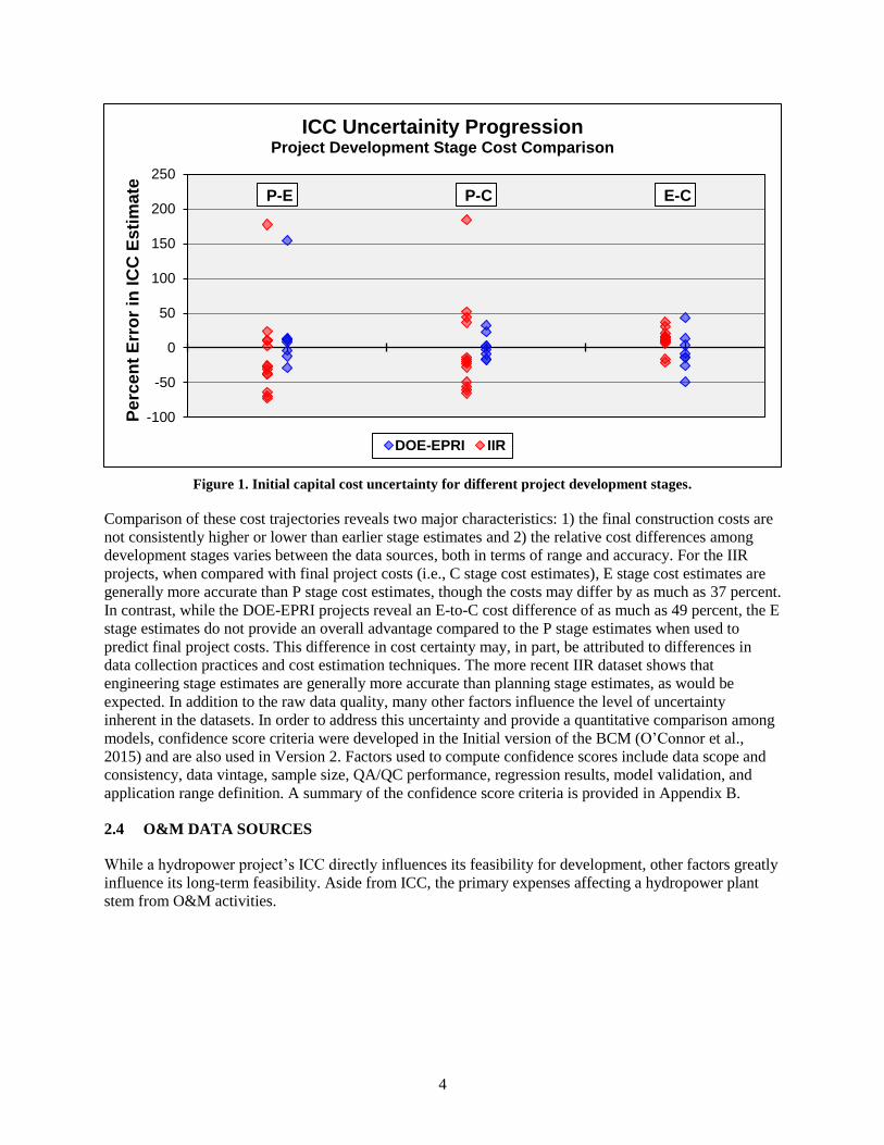
construction stage). Figure 1 illustrates this uncertainty for 8 DOE-EPRI projects and 13 IIR projects for

which planning (P), engineering (E), and construction (C) data were available

4

Figure 1. Initial capital cost uncertainty for different project development stages.

Comparison of these cost trajectories reveals two major characteristics: 1) the final construction costs are

not consistently higher or lower than earlier stage estimates and 2) the relative cost differences among

development stages varies between the data sources, both in terms of range and accuracy. For the IIR

projects, when compared with final project costs (i.e., C stage cost estimates), E stage cost estimates are

generally more accurate than P stage cost estimates, though the costs may differ by as much as 37 percent.

In contrast, while the DOE-EPRI projects reveal an E-to-C cost difference of as much as 49 percent, the E

stage estimates do not provide an overall advantage compared to the P stage estimates when used to

predict final project costs. This difference in cost certainty may, in part, be attributed to differences in

data collection practices and cost estimation techniques. The more recent IIR dataset shows that

engineering stage estimates are generally more accurate than planning stage estimates, as would be

expected. In addition to the raw data quality, many other factors influence the level of uncertainty

inherent in the datasets. In order to address this uncertainty and provide a quantitative comparison among

models, confidence score criteria were developed in the Initial version of the BCM (O’Connor et al.,

2015) and are also used in Version 2. Factors used to compute confidence scores include data scope and

consistency, data vintage, sample size, QA/QC performance, regression results, model validation, and

application range definition. A summary of the confidence score criteria is provided in Appendix B.

2.4 O&M DATA SOURCES

While a hydropower project’s ICC directly influences its feasibility for development, other factors greatly

influence its long-term feasibility. Aside from ICC, the primary expenses affecting a hydropower plant

stem from O&M activities.

P-E P-C E-C

-100

-50

0

50

100

150

200

250

Pe

rce

nt

Err

or

in I

CC

Es

tim

ate

ICC Uncertainity Progression

Project Development Stage Cost Comparison

DOE-EPRI IIR

5

In order to evaluate O&M costs and develop BCMs for U.S. hydropower plants, annual plant O&M data

for 1994-2013 were collected from the FERC Form 1 database (FERC, 2015) for a total of 315 plants.

Under FERC regulation, electric utilities or other entities classified as Major1 are required to annually

submit financial and operational information through Form 1. Ultimately this limits the O&M cost data

sample to those projects controlled by Investor Owned Utilities (IOUs), municipalities, Public Utility

Districts (PUDs), and other owners with load-serving or transmission obligations.

The following categories of expenses are included in Form 1 and combine to form total annual expense:

Operation Expenses Engineering Expenses

Water Power Expenses Structures Expenses

Hydraulic Expenses Dams Expenses

Electric Expenses Plant Expenses

Generation Expenses Miscellaneous Plant Expenses

Rent Expenses

While the instructions for completing Form 1 help to standardize submittals, the data tend to suffer from

several shortcomings which impact accuracy and modeling capability. Among these are 1) accounting

inconsistencies within and across organizations, 2) partial plant ownership which may segregate data

submittal, and 3) bias potential due to the plant subset for which Form 1 data submittals are required—

hydropower owners without directly owned transmission system assets, such as, generating companies,

independent power producers and industrial users, as well as the United States Army Corps of Engineers

and the Bureau of Reclamation may employ alternative O&M strategies with differing costs and results.

To the extent possible, these issues have been addressed during the screening process (described in

Section 5), though the subset of plant data included in the dataset may suffer from selection bias. Out of

the roughly 80 GW of conventional hydropower across the U.S., the 2013 Form 1 dataset contains 212

plants totaling 14.5 GW (18%).

2.5 ENVIRONMENTAL MITIGATION AND LICENSING

FERC issues preliminary permits, licenses, relicenses (or in some cases grants exemptions), and

environmental impact statements for the vast majority of non-federal hydropower projects. In applications

for original or new licenses, most major projects above 5 MW are required to submit actual or

approximate original cost2. Major water projects whose installed capacity is less than 5 MW and minor

water projects of less than 1.5 MW must include the estimated cost of the project and of each proposed

environmental mitigation measure3. This cost data is typically available in itemized form in a project’s

Environmental Impact Statement (EIS). In addition to the cost of proposed mitigation measures, the EIS

also contains the licensee’s application preparation costs inclusive of the costs of required studies as

reported to FERC. Preliminary permits typically do not include useful cost information, but may at times

provide cost estimates for the studies to be performed before applying for a full license.

These data collection efforts are ongoing, and additional work is still being conducted to finalize

mitigation and licensing BCMs. As a stop-gap measure historical environmental mitigation and licensing

1 Per FERC classification, Major refers to utilities and licensees that had, in each of the last three consecutive years, sales or

transmission service that exceeded any one or more of the following:

(a) One million megawatt-hours of total sales;

(b) 100 megawatt-hours of sales for resale;

(c) 500 megawatt-hours of power exchanges delivered; or

(d) 500 megawatt-hours of wheeling for others (deliveries plus losses). 2 This information is found in a License application’s “Exhibit D” and/or “Exhibit A”

3 This information is found in a License application’s “Exhibit A”

6

cost tools are reproduced from previous work done by Idaho National Laboratory (INL, 2003) study. The

cost model equations, both in the original form and in an escalated form for present-day use, are provided

in Section 4 with a discussion of the source data and application limitations.

3. HISTORICAL DATA TRENDS

3.1 CAPITAL EXPENDITURE

Examining the subset of cost data collected from those projects that have either been constructed or are

actively under construction (c-stage) in the U.S. provides insight into the relative economics of modern

hydropower development. In order to demonstrate historical cost distributions, the ORNL ICC database

was screened to identify completed or actively under construction projects for which the final ICC4 was

known. Projects were categorized based on resource type (NPD, NSD and Canal/Conduit), while NPDs

were further grouped into Low Head and High Head NPDs based on hydraulic head. Low Head NPDs are

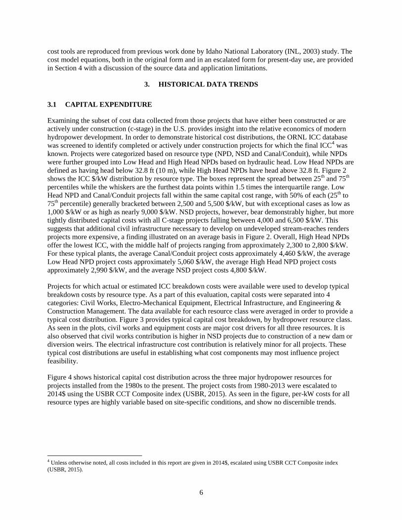
defined as having head below 32.8 ft (10 m), while High Head NPDs have head above 32.8 ft. Figure 2

shows the ICC $/kW distribution by resource type. The boxes represent the spread between 25th and 75

th

percentiles while the whiskers are the furthest data points within 1.5 times the interquartile range. Low

Head NPD and Canal/Conduit projects fall within the same capital cost range, with 50% of each (25th to

75th percentile) generally bracketed between 2,500 and 5,500 $/kW, but with exceptional cases as low as

1,000 $/kW or as high as nearly 9,000 $/kW. NSD projects, however, bear demonstrably higher, but more

tightly distributed capital costs with all C-stage projects falling between 4,000 and 6,500 $/kW. This

suggests that additional civil infrastructure necessary to develop on undeveloped stream-reaches renders

projects more expensive, a finding illustrated on an average basis in Figure 2. Overall, High Head NPDs

offer the lowest ICC, with the middle half of projects ranging from approximately 2,300 to 2,800 $/kW.

For these typical plants, the average Canal/Conduit project costs approximately 4,460 $/kW, the average

Low Head NPD project costs approximately 5,060 $/kW, the average High Head NPD project costs

approximately 2,990 $/kW, and the average NSD project costs 4,800 $/kW.

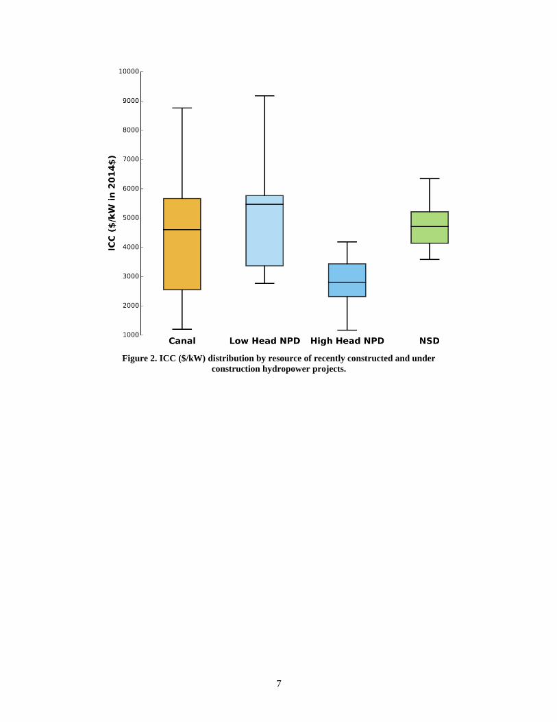
Projects for which actual or estimated ICC breakdown costs were available were used to develop typical

breakdown costs by resource type. As a part of this evaluation, capital costs were separated into 4

categories: Civil Works, Electro-Mechanical Equipment, Electrical Infrastructure, and Engineering &

Construction Management. The data available for each resource class were averaged in order to provide a

typical cost distribution. Figure 3 provides typical capital cost breakdown, by hydropower resource class.

As seen in the plots, civil works and equipment costs are major cost drivers for all three resources. It is

also observed that civil works contribution is higher in NSD projects due to construction of a new dam or

diversion weirs. The electrical infrastructure cost contribution is relatively minor for all projects. These

typical cost distributions are useful in establishing what cost components may most influence project

feasibility.

Figure 4 shows historical capital cost distribution across the three major hydropower resources for

projects installed from the 1980s to the present. The project costs from 1980-2013 were escalated to

2014$ using the USBR CCT Composite index (USBR, 2015). As seen in the figure, per-kW costs for all

resource types are highly variable based on site-specific conditions, and show no discernible trends.

4 Unless otherwise noted, all costs included in this report are given in 2014$, escalated using USBR CCT Composite index

(USBR, 2015).

7

Figure 2. ICC ($/kW) distribution by resource of recently constructed and under

construction hydropower projects.

8

Figure 3. ICC ($/kW) breakdown by resource of recently constructed and under construction hydropower

projects.

41% 49%

43%

50%

34%

37%

34%

26%

3%

5%

10%

8% 22%

9%

13%

16%

0

1,000

2,000

3,000

4,000

5,000

Canal Low Head NPD High Head NPD NSD

ICC

($

/kW

in

20

14

$)

Historical Average ICC Breakdown By Resource Type

Eng. & Const. Management Electrical Infrastructure

Elect.-Mech. Equipment Civil Works

5060 $/kW

2990 $/kW

4460 $/kW

4800 $/kW

9

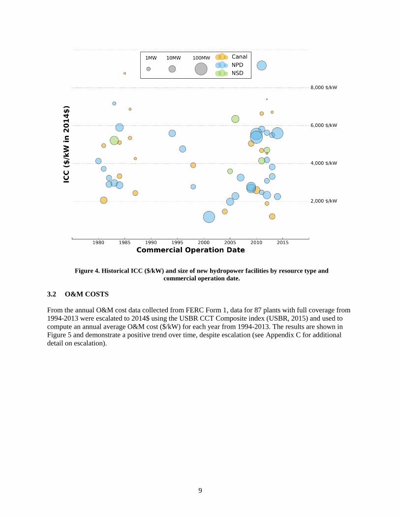
Figure 4. Historical ICC ($/kW) and size of new hydropower facilities by resource type and

commercial operation date.

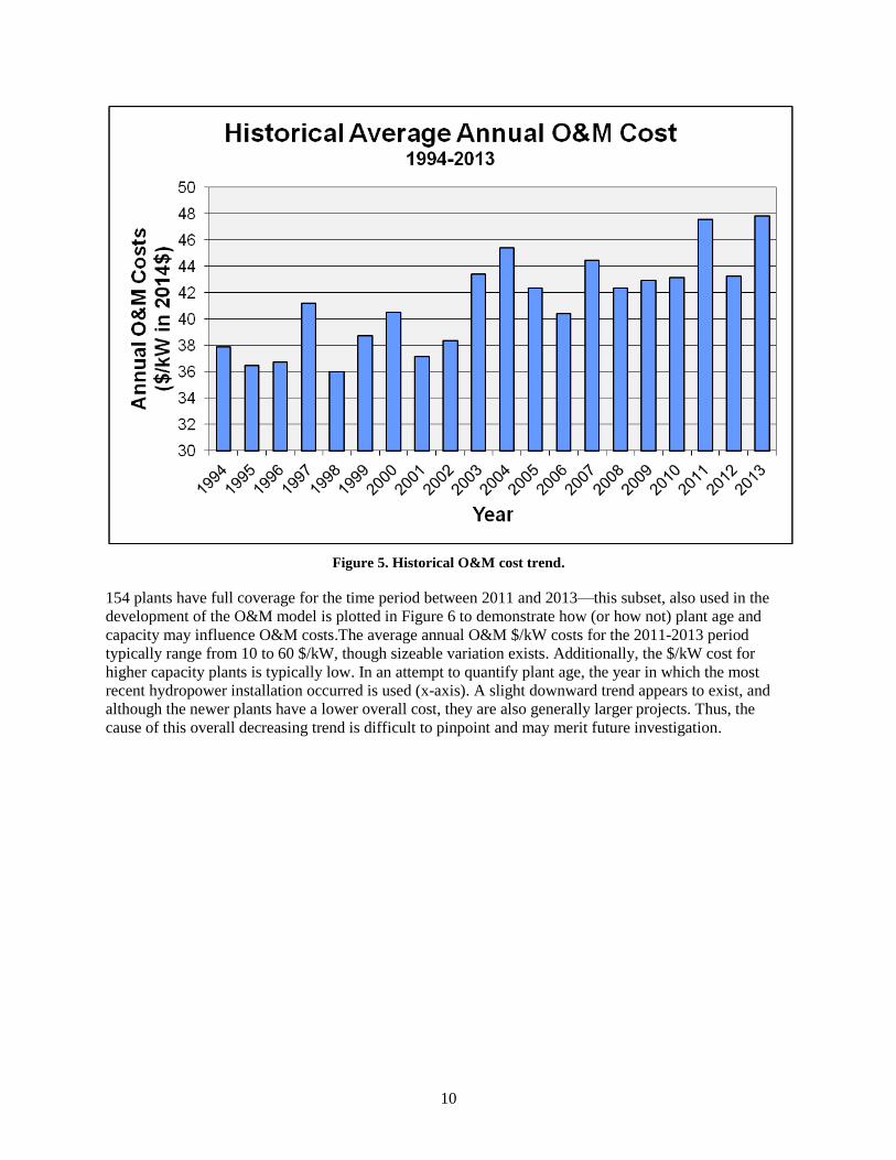
3.2 O&M COSTS

From the annual O&M cost data collected from FERC Form 1, data for 87 plants with full coverage from

1994-2013 were escalated to 2014$ using the USBR CCT Composite index (USBR, 2015) and used to

compute an annual average O&M cost ($/kW) for each year from 1994-2013. The results are shown in

Figure 5 and demonstrate a positive trend over time, despite escalation (see Appendix C for additional

detail on escalation).

10

Figure 5. Historical O&M cost trend.

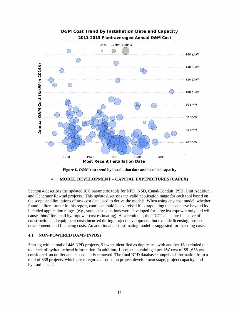
154 plants have full coverage for the time period between 2011 and 2013—this subset, also used in the

development of the O&M model is plotted in Figure 6 to demonstrate how (or how not) plant age and

capacity may influence O&M costs.The average annual O&M $/kW costs for the 2011-2013 period

typically range from 10 to 60 $/kW, though sizeable variation exists. Additionally, the $/kW cost for

higher capacity plants is typically low. In an attempt to quantify plant age, the year in which the most

recent hydropower installation occurred is used (x-axis). A slight downward trend appears to exist, and

although the newer plants have a lower overall cost, they are also generally larger projects. Thus, the

cause of this overall decreasing trend is difficult to pinpoint and may merit future investigation.

11

Figure 6. O&M cost trend by installation date and installed capacity

4. MODEL DEVELOPMENT – CAPITAL EXPENDITURES (CAPEX)

Section 4 describes the updated ICC parametric tools for NPD, NSD, Canal/Conduit, PSH, Unit Addition,

and Generator Rewind projects. This update discusses the valid application range for each tool based on

the scope and limitations of raw cost data used to derive the models. When using any cost model, whether

found in literature or in this report, caution should be exercised if extrapolating the cost curve beyond its

intended application ranges (e.g., some cost equations were developed for large hydropower only and will

cause “bias” for small hydropower cost estimating). As a reminder, the “ICC” data are inclusive of

construction and equipment costs incurred during project development, but exclude licensing, project

development, and financing costs. An additional cost estimating model is suggested for licensing costs.

4.1 NON-POWERED DAMS (NPDS)

Starting with a total of 446 NPD projects, 91 were identified as duplicates, with another 16 excluded due

to a lack of hydraulic head information. In addition, 1 project containing a per-kW cost of $81,653 was

considered an outlier and subsequently removed. The final NPD database comprises information from a

total of 338 projects, which are categorized based on project development stage, project capacity, and

hydraulic head.

12

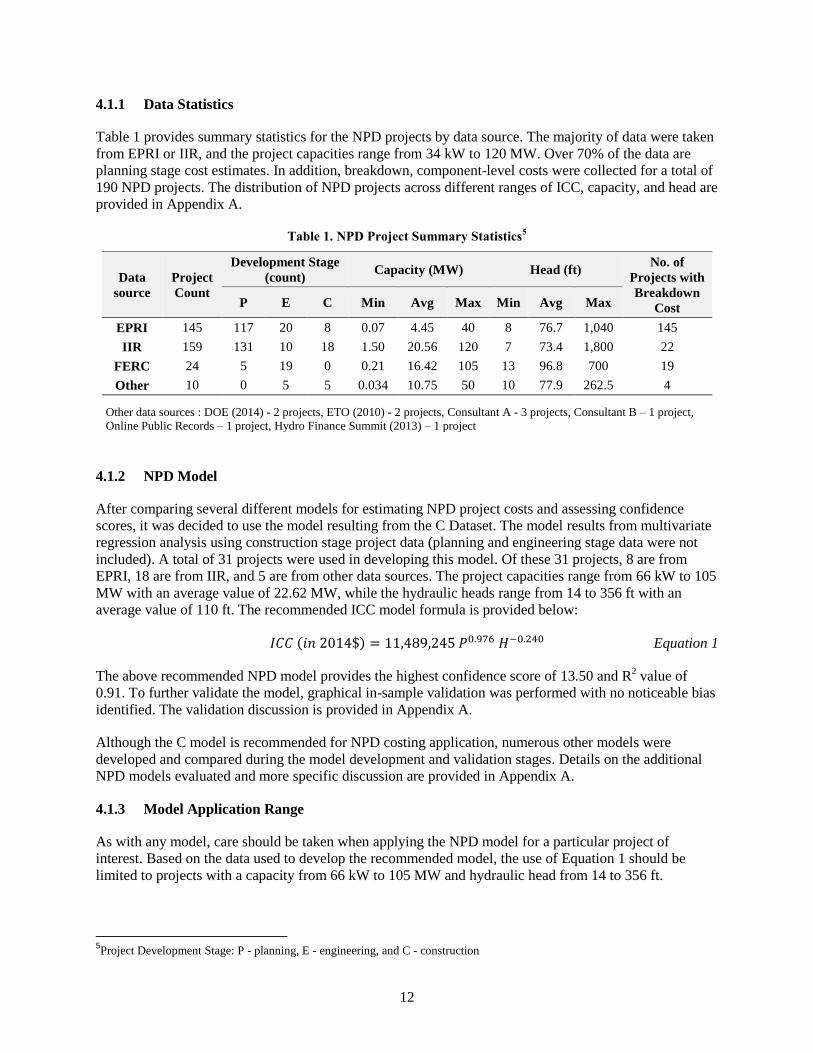
4.1.1 Data Statistics

Table 1 provides summary statistics for the NPD projects by data source. The majority of data were taken

from EPRI or IIR, and the project capacities range from 34 kW to 120 MW. Over 70% of the data are

planning stage cost estimates. In addition, breakdown, component-level costs were collected for a total of

190 NPD projects. The distribution of NPD projects across different ranges of ICC, capacity, and head are

provided in Appendix A.

Table 1. NPD Project Summary Statistics5

Data

source

Project

Count

Development Stage

(count) Capacity (MW) Head (ft)

No. of

Projects with

Breakdown

Cost P E C Min Avg Max Min Avg Max

EPRI 145 117 20 8 0.07 4.45 40 8 76.7 1,040 145

IIR 159 131 10 18 1.50 20.56 120 7 73.4 1,800 22

FERC 24 5 19 0 0.21 16.42 105 13 96.8 700 19

Other 10 0 5 5 0.034 10.75 50 10 77.9 262.5 4

Other data sources : DOE (2014) - 2 projects, ETO (2010) - 2 projects, Consultant A - 3 projects, Consultant B – 1 project,

Online Public Records – 1 project, Hydro Finance Summit (2013) – 1 project

4.1.2 NPD Model

After comparing several different models for estimating NPD project costs and assessing confidence

scores, it was decided to use the model resulting from the C Dataset. The model results from multivariate

regression analysis using construction stage project data (planning and engineering stage data were not

included). A total of 31 projects were used in developing this model. Of these 31 projects, 8 are from

EPRI, 18 are from IIR, and 5 are from other data sources. The project capacities range from 66 kW to 105

MW with an average value of 22.62 MW, while the hydraulic heads range from 14 to 356 ft with an

average value of 110 ft. The recommended ICC model formula is provided below:

𝐼𝐶𝐶 (𝑖𝑛 2014$) = 11,489,245 𝑃0.976 𝐻−0.240 Equation 1

The above recommended NPD model provides the highest confidence score of 13.50 and R2 value of

0.91. To further validate the model, graphical in-sample validation was performed with no noticeable bias

identified. The validation discussion is provided in Appendix A.

Although the C model is recommended for NPD costing application, numerous other models were

developed and compared during the model development and validation stages. Details on the additional

NPD models evaluated and more specific discussion are provided in Appendix A.

4.1.3 Model Application Range

As with any model, care should be taken when applying the NPD model for a particular project of

interest. Based on the data used to develop the recommended model, the use of Equation 1 should be

limited to projects with a capacity from 66 kW to 105 MW and hydraulic head from 14 to 356 ft.

5Project Development Stage: P - planning, E - engineering, and C - construction

13

4.2 NEW STREAM-REACH DEVELOPMENT (NSDS)

Starting with a total of 98 NSD projects, 3 were identified as duplicates, with another 2 excluded due to a

lack of hydraulic head information. In addition, 1 project containing a per-kW cost of $100,485 was

considered an outlier and subsequently removed. The final NSD database comprises information from a

total of 92 projects, which are categorized based on project development stage, project capacity, and

hydraulic head.


Table 2 provides summary statistics for the NSD projects by data source. The majority of data were taken

from IIR, and the project capacities range from 163 kW to 824 MW. Over 60% of the data contain

planning stage development costs. In addition, breakdown costs were collected for a total of 33 NSD

projects. The distribution of NSD projects across different ranges of ICC, capacity, and head are provided

in Appendix A.

Table 2. NSD Project Summary Statistics6

Data

source

Project

Count

Development Stage


No. of

Projects with

Breakdown


EPRI 18 15 2 1 0.163 4.25 24 10 68.4 313 18

IIR 44 40 1 3 3.0 48.28 600 20.5 766.5 3050 6

FERC 7 2 5 0 0.40 52.77 121.5 56.5 308.6 965.5 5

Other 23 0 9 14 0.50 64 824 10 533.7 1896.3 4

Other data sources : Consultant A – 3 projects, Consultant B – 18 projects, TVA (1941) – 1 project, Online Public Records - 1

project.

4.2.2 NSD Model

After comparing several different models for estimating NSD project costs and assessing confidence

scores, it was decided to use the model resulting from the C Dataset. The model results from multivariate

regression analysis using construction stage project data (planning and engineering stage data were not

included). A total of 18 projects were used in developing this model. Of these 18 projects, 1 is from EPRI,

3 are from IIR, and 14 are from other data sources. The project capacities range from 3 to 824 MW with

an average value of 80.80 MW, while the hydraulic heads range from 19.3 to 1896 ft with an average

value of 790.07 ft. The recommended ICC model formula is provided below:


The above recommended NSD model provides the highest confidence score of 12.70 and R2 value of

0.96. To further validate the model, graphical in-sample validation was performed with no noticeable bias


Although the C model is recommended for NSD costing application, numerous other models were

developed and compared during the model development and validation stages. Details on the additional

NPD models evaluated and more specific discussion are provided in Appendix A.


14


As with any model, care should be taken when applying the NSD model for a particular project of

interest. Based on the data used to develop the recommended model, the use of Equation 2 should be

limited to projects with a capacity from 3 to 824 MW and hydraulic head from 19.3 to 1896 ft.

4.3 CANAL/CONDUITS

Starting with a total of 117 Canal/Conduit projects, 11 were identified as duplicates, with another 6

excluded due to a lack of cost information. In addition, 1 project with a very high capacity of 150 MW

was identified as an outlier and subsequently removed. The final Canal/Conduit database comprises

information from a total of 99 projects, which are categorized based on project development stage, project

capacity, and hydraulic head.


Table 3 provides summary statistics for the Canal/Conduit projects by data source. The majority of data

were taken from other resources, and the project capacities range from 10 kW to 15 MW. Breakdown

costs were collected for a total of 75 Canal/Conduit projects. The distribution of Canal/Conduit projects

across different ranges of ICC, capacity, and head are provided in Appendix A.

Table 3. Canal/Conduit Project Summary Statistics7

Data

source

Project

Count

Development Stage


No. of Projects

with

Breakdown


EPRI 34 29 1 4 0.10 2.24 15 21 179.5 904.0 34

IIR 4 3 0 1 1.0 5.65 13 146 689.3 1971.0 1

FERC 9 4 5 0 0.23 1.72 6.15 33.5 211.2 445.0 5

Other 52 1 36 15 0.01 1.10 7.15 5 234.9 1847.0 35

Other data sources : Consultant D – 1 project, City of Boulder (2013) – 8 projects, COID (2011) – 5 projects, Consultant C – 1

project, ETO (2010) – 24 projects, NUID (2009) – 4 projects, Butterfield (2011) – 1 project, Online Public Records – 8

projects.

4.3.2 Canal/Conduit Model

After comparing several different models for estimating Canal/Conduit project costs and assessing

confidence scores, it was decided to use the model resulting from the EC Dataset. The model results from

multivariate regression analysis using engineering and construction stage project data (planning stage data

were not included). A total of 62 projects were used in developing this model. Of these 62 projects, 5 are

from EPRI, 1 is from IIR, 5 are from FERC and 51 are from other data sources. The project capacities

range from 10.5 kW to 13 MW with an average value of 1.63 MW, while the hydraulic heads range from

5 to 1847 ft with an average value of 209.6 ft. The recommended ICC model formula is provided below:



15

The above recommended Canal/Conduit model provides the highest confidence score of 12.57 and R2

value of 0.77. To further validate the model, graphical in-sample validation was performed with no

noticeable bias identified. The validation discussion is provided in Appendix A.

Although the EC model is recommended for Canal/Conduit costing application, numerous other models

were developed and compared during the model development and validation stages. Details on the

additional Canal/Conduit models evaluated and more specific discussion are provided in Appendix A.


As with any model, care should be taken when applying the Canal/Conduit model for a particular project

of interest. Based on the data used to develop the recommended model, the use of Equation 3 should be

limited to projects with a capacity from 10 kW to 13 MW and hydraulic head from 5 to 1,847 ft.

4.4 PUMPED STORAGE HYDROPOWER (PSH)

4.4.1 PSH Data Uncertainty

Starting with a total of 151 PSH projects, 16 were non-U.S. data points, 2 were identified as different

projects (existing/upgrade), with another 16 excluded as duplicates. Another 6 projects were removed due

to lack of capital cost or hydraulic head information. One project with a cost of 11,000 $/kW was

removed as an outlier. Additionally, all 14 projects with construction stage data were removed—these

projects are existing U.S. projects, and even when escalated using the USBR CCT Composite index

(USBR, 2015), were substantially less expensive on a per-kW basis than the remainder of the dataset. As

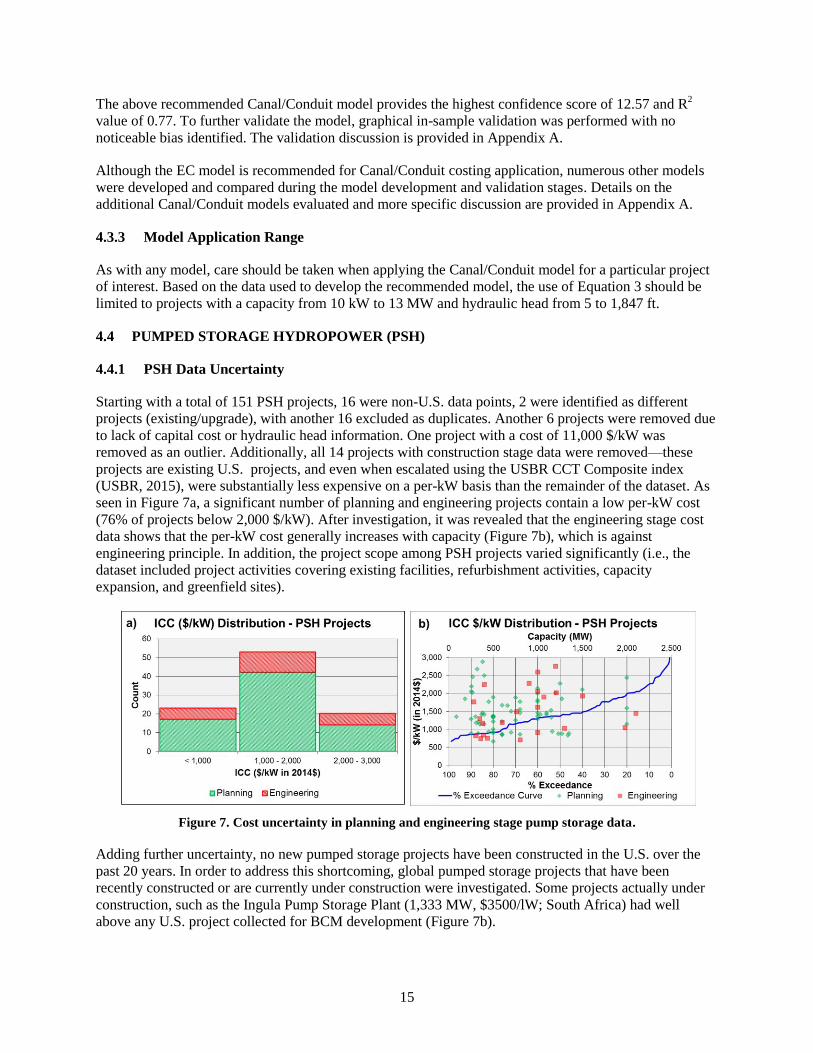
seen in Figure 7a, a significant number of planning and engineering projects contain a low per-kW cost

(76% of projects below 2,000 $/kW). After investigation, it was revealed that the engineering stage cost

data shows that the per-kW cost generally increases with capacity (Figure 7b), which is against

engineering principle. In addition, the project scope among PSH projects varied significantly (i.e., the

dataset included project activities covering existing facilities, refurbishment activities, capacity

expansion, and greenfield sites).

Figure 7. Cost uncertainty in planning and engineering stage pump storage data.

Adding further uncertainty, no new pumped storage projects have been constructed in the U.S. over the

past 20 years. In order to address this shortcoming, global pumped storage projects that have been

recently constructed or are currently under construction were investigated. Some projects actually under

construction, such as the Ingula Pump Storage Plant (1,333 MW, $3500/lW; South Africa) had well

above any U.S. project collected for BCM development (Figure 7b).

16

As discussed in Section 2, the relatively low certainty associated with planning and engineering stage data

would present reliability issues for a P-E model. Due to data limitations and inconsistencies between

collected cost data, it was decided that no PSH model be recommended from the BCM collection process.

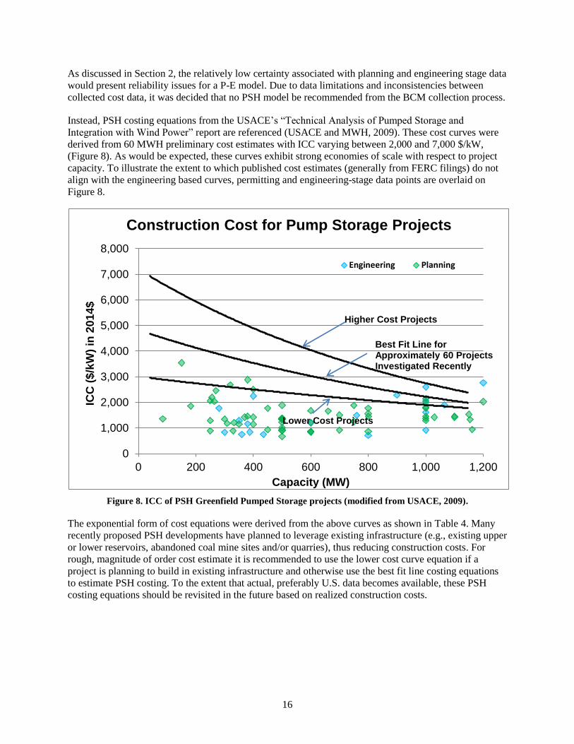
Instead, PSH costing equations from the USACE’s “Technical Analysis of Pumped Storage and

Integration with Wind Power” report are referenced (USACE and MWH, 2009). These cost curves were

derived from 60 MWH preliminary cost estimates with ICC varying between 2,000 and 7,000 $/kW,

(Figure 8). As would be expected, these curves exhibit strong economies of scale with respect to project

capacity. To illustrate the extent to which published cost estimates (generally from FERC filings) do not

align with the engineering based curves, permitting and engineering-stage data points are overlaid on

Figure 8.

Figure 8. ICC of PSH Greenfield Pumped Storage projects (modified from USACE, 2009).

The exponential form of cost equations were derived from the above curves as shown in Table 4. Many

recently proposed PSH developments have planned to leverage existing infrastructure (e.g., existing upper

or lower reservoirs, abandoned coal mine sites and/or quarries), thus reducing construction costs. For

rough, magnitude of order cost estimate it is recommended to use the lower cost curve equation if a

project is planning to build in existing infrastructure and otherwise use the best fit line costing equations

to estimate PSH costing. To the extent that actual, preferably U.S. data becomes available, these PSH

costing equations should be revisited in the future based on realized construction costs.

0

1,000

2,000

3,000

4,000

5,000

6,000

7,000

8,000

0 200 400 600 800 1,000 1,200

ICC

($

/kW

) in

20

14

$

Capacity (MW)

Construction Cost for Pump Storage Projects

Engineering Planning

Higher Cost Projects

Best Fit Line for Approximately 60 Projects Investigated Recently

Lower Cost Projects

17

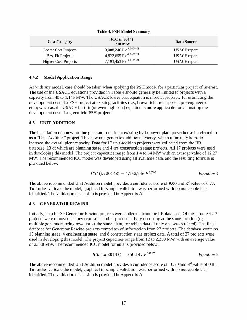
Table 4. PSH Model Summary

Cost Category ICC in 2014$

P in MW Data Source

Lower Cost Projects 3,008,246 P e-0.000460P

USACE report

Best Fit Projects 4,822,655 P e-0.000776P

USACE report

Higher Cost Projects 7,193,453 P e-0.000963P

USACE report


As with any model, care should be taken when applying the PSH model for a particular project of interest.

The use of the USACE equations provided in Table 4 should generally be limited to projects with a

capacity from 40 to 1,145 MW. The USACE lower cost equation is more appropriate for estimating the

development cost of a PSH project at existing facilities (i.e., brownfield, repurposed, pre-engineered,

etc.); whereas, the USACE best fit (or even high cost) equation is more applicable for estimating the

development cost of a greenfield PSH project.

4.5 UNIT ADDITION

The installation of a new turbine generator unit in an existing hydropower plant powerhouse is referred to

as a “Unit Addition” project. This new unit generates additional energy, which ultimately helps to

increase the overall plant capacity. Data for 17 unit addition projects were collected from the IIR

database, 13 of which are planning stage and 4 are construction stage projects. All 17 projects were used

in developing this model. The project capacities range from 1.4 to 64 MW with an average value of 12.27

MW. The recommended ICC model was developed using all available data, and the resulting formula is

provided below:

𝐼𝐶𝐶 (𝑖𝑛 2014$) = 4,163,746 𝑃0.741 Equation 4

The above recommended Unit Addition model provides a confidence score of 9.00 and R2 value of 0.77.

To further validate the model, graphical in-sample validation was performed with no noticeable bias


4.6 GENERATOR REWIND

Initially, data for 30 Generator Rewind projects were collected from the IIR database. Of these projects, 3

projects were removed as they represent similar project activity occurring at the same location (e.g.,

multiple generators being rewound at the same plant, for which data of only one was retained). The final

database for Generator Rewind projects comprises of information from 27 projects. The database contains

15 planning stage, 4 engineering stage, and 8 construction stage project data. A total of 27 projects were

used in developing this model. The project capacities range from 12 to 2,250 MW with an average value

of 236.8 MW. The recommended ICC model formula is provided below:

𝐼𝐶𝐶 (𝑖𝑛 2014$) = 250,147 𝑃0.817 Equation 5

The above recommended Unit Addition model provides a confidence score of 10.70 and R2 value of 0.81.



18

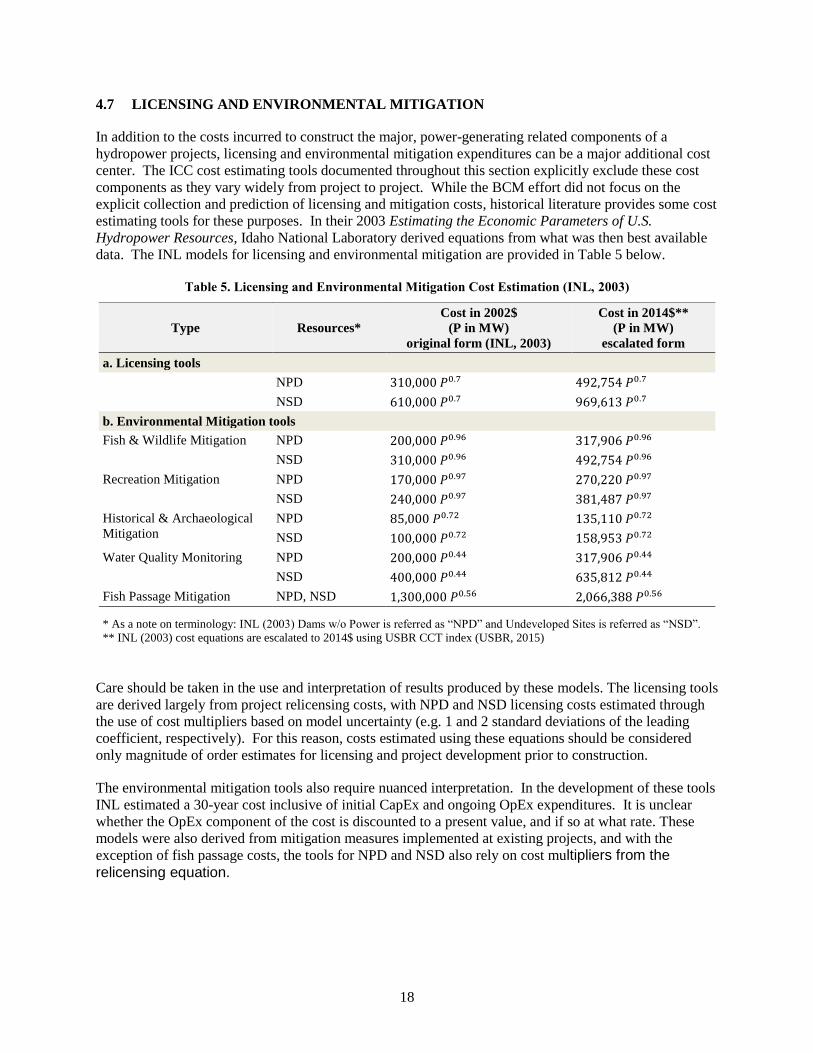
4.7 LICENSING AND ENVIRONMENTAL MITIGATION

In addition to the costs incurred to construct the major, power-generating related components of a

hydropower projects, licensing and environmental mitigation expenditures can be a major additional cost

center. The ICC cost estimating tools documented throughout this section explicitly exclude these cost

components as they vary widely from project to project. While the BCM effort did not focus on the

explicit collection and prediction of licensing and mitigation costs, historical literature provides some cost

estimating tools for these purposes. In their 2003 Estimating the Economic Parameters of U.S.

Hydropower Resources, Idaho National Laboratory derived equations from what was then best available

data. The INL models for licensing and environmental mitigation are provided in Table 5 below.

Table 5. Licensing and Environmental Mitigation Cost Estimation (INL, 2003)

Type Resources*

Cost in 2002$

(P in MW)

original form (INL, 2003)

Cost in 2014$**

(P in MW)

escalated form

a. Licensing tools

NPD 310,000 𝑃0.7 492,754 𝑃0.7

NSD 610,000 𝑃0.7 969,613 𝑃0.7

b. Environmental Mitigation tools

Fish & Wildlife Mitigation NPD 200,000 𝑃0.96 317,906 𝑃0.96

NSD 310,000 𝑃0.96 492,754 𝑃0.96

Recreation Mitigation NPD 170,000 𝑃0.97 270,220 𝑃0.97

NSD 240,000 𝑃0.97 381,487 𝑃0.97

Historical & Archaeological

Mitigation

NPD 85,000 𝑃0.72 135,110 𝑃0.72

NSD 100,000 𝑃0.72 158,953 𝑃0.72

Water Quality Monitoring NPD 200,000 𝑃0.44 317,906 𝑃0.44

NSD 400,000 𝑃0.44 635,812 𝑃0.44

Fish Passage Mitigation NPD, NSD 1,300,000 𝑃0.56 2,066,388 𝑃0.56

* As a note on terminology: INL (2003) Dams w/o Power is referred as “NPD” and Undeveloped Sites is referred as “NSD”.

** INL (2003) cost equations are escalated to 2014$ using USBR CCT index (USBR, 2015)

Care should be taken in the use and interpretation of results produced by these models. The licensing tools

are derived largely from project relicensing costs, with NPD and NSD licensing costs estimated through

the use of cost multipliers based on model uncertainty (e.g. 1 and 2 standard deviations of the leading

coefficient, respectively). For this reason, costs estimated using these equations should be considered

only magnitude of order estimates for licensing and project development prior to construction.

The environmental mitigation tools also require nuanced interpretation. In the development of these tools

INL estimated a 30-year cost inclusive of initial CapEx and ongoing OpEx expenditures. It is unclear

whether the OpEx component of the cost is discounted to a present value, and if so at what rate. These

models were also derived from mitigation measures implemented at existing projects, and with the

exception of fish passage costs, the tools for NPD and NSD also rely on cost multipliers from the

relicensing equation.

19

5. RESULTS – OPERATIONAL EXPENDITURES (OPEX)

Recent and historical investigations into operations and & maintenance (O&M) costs specific to

hydropower have demonstrated that costs can be relatively low compared to other technologies and scale

with the size of the project (INL, 2003; EPRI, 2011; IRENA, 2015). The findings from these historical

reports are useful in guiding O&M model development; however, a comprehensive approach was taken to

consider a wide array of potential model forms.

5.1 DATA MANAGEMENT

As the data collected from FERC Form 1 to develop the O&M models spans two decades, it is important

to accurately adjust the historical cost data using escalation. While many different cost and inflation

indexes exist for these purposes, comparison of the raw O&M expense data with a suite of different cost

indexes resulted in the USBR CCT Composite index being selected for escalation. This index, which was

also used for ICC escalation, provided a relatively good fit to the O&M data and allowed for escalation to

2014$ (see Appendix C for additional detail on escalation) .

To ensure accuracy in the final O&M database, several layers of QA/QC were performed. Due to the

potential for data entry error, generation data were assessed to identify inconsistency. The major source of

inconsistency identified was in the unit of measure used to report generation (i.e., where the generation

value was obviously reported in MWh instead of kWh). For instances in which the source of

inconsistency was easily identifiable and objective, the raw data were corrected; however, for

inconsistencies which could not be identified with certainty, the records were removed. After correcting

the raw data, screening was performed to improve data quality for use in regression modeling. As with the

ICC models, the O&M models were developed using log transformed linear regression with bias

correction (O’Connor et al., 2015)

Within the database, screening criteria included removing:

1. Any record containing a zero or negative value for total O&M expenses.

2. Any plant for which one or more years of total annual O&M expenses were unavailable during the

period of analysis.

3. Any record containing a zero or negative value for net generation8.

4. Any record containing a zero or negative value for total capacity.

5. Any plant for which the reported total capacity values varied by more than 5% over the period of

interest.

6. Any plant for which the head could not be determined.

In addition, the dataset’s multi-year average capacity value was compared with the NHAAP-reported

capacity for each plant to identify discrepancies. Plants were removed from the final dataset if the

discrepancies were large enough to be of concern to staff. Although not explicitly defined, the results of

this screening process removed any plants for which the Form 1 and NHAAP capacity values differed by

more than 5%.

8 This is in addition to the exclusion of data from PSH plants, which is stored in a different table in FERC Form-1, and were not

commingled with the conventional hydropower dataset

20

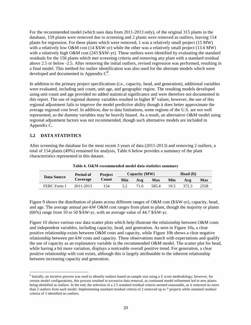
For the recommended model (which uses data from 2011-2013 only), of the original 315 plants in the

database, 159 plants were removed due to screening and 2 plants were removed as outliers, leaving 154

plants for regression. For these plants which were removed, 1 was a relatively small project (15 MW)

with a relatively low O&M cost (14 $/kW-yr) while the other was a relatively small project (13.6 MW)

with a relatively high O&M cost (243 $/kW-yr). These outliers were identified by evaluating the standard

residuals for the 156 plants which met screening criteria and removing any plant with a standard residual

above 2.5 or below -2.5. After removing the initial outliers, revised regression was performed, resulting in

a final model. This method for outlier identification was also used for the alternate models which were

developed and documented in Appendix C9.

In addition to the primary project specifications (i.e., capacity, head, and generation), additional variables

were evaluated, including unit count, unit age, and geographic region. The resulting models developed

using unit count and age provided no added statistical significance and were therefore not documented in

this report. The use of regional dummy variables resulted in higher R2 values; however, the use of this

regional adjustment fails to improve the model predictive ability though it does better approximate the

average regional cost level. In addition, due to data limitations, some regions of the U.S. are not well

represented, so the dummy variables may be heavily biased. As a result, an alternative O&M model using

regional adjustment factors was not recommended, though such alternative models are included in

Appendix C.

5.2 DATA STATISTICS

After screening the database for the most recent 3 years of data (2011-2013) and removing 2 outliers, a

total of 154 plants (49%) remained for analysis, Table 6 below provides a summary of the plant

characteristics represented in this dataset.

Table 6. O&M recommended model data statistics summary

Data Source Period of

Coverage

Project

Count

Capacity (MW) Head (ft)

Min Avg Max Min Avg Max

FERC Form 1 2011-2013 154 3.2 71.6 585.4 19.5 372.3 2558

Figure 9 shows the distribution of plants across different ranges of O&M cost ($/kW-yr), capacity, head,

and age. The average annual per-kW O&M cost ranges from plant to plant, though the majority or plants

(66%) range from 10 to 50 $/kW-yr, with an average value of 44.7 $/kW-yr.

Figure 10 shows various raw data scatter plots which help illustrate the relationship between O&M costs

and independent variables, including capacity, head, and generation. As seen in Figure 10a, a clear

positive relationship exists between O&M costs and capacity, while Figure 10b shows a clear negative

relationship between per-kW costs and capacity. These observations match with expectations and qualify

the use of capacity as an explanatory variable in the recommended O&M model. The scatter plot for head,

while having a bit more variation, displays a noticeable overall positive trend. For generation, a clear

positive relationship with cost exists, although this is largely attributable to the inherent relationship

between increasing capacity and generation.

9 Initially, an iterative process was used to identify outliers based on sample size using a Z score methodology; however, for

certain model configurations, this process resulted in excessive data removal, as continued model refinement led to new plants

being identified as outliers. In the end, the selection of a 2.5 standard residual criteria seemed reasonable, as it removed no more

than 2 outliers from each model. Implementing standard residual criteria of 2 removed up to 7 projects while standard residual

criteria of 3 identified no outliers.

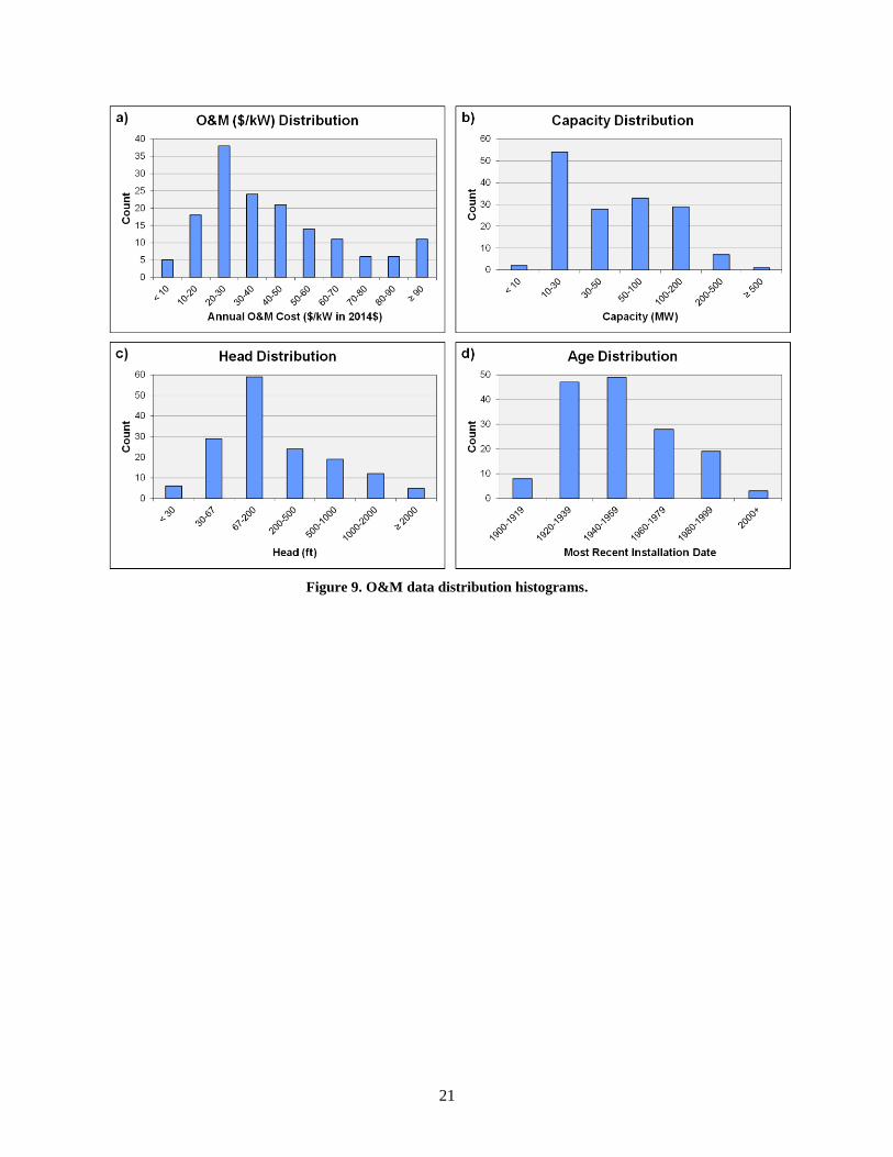
21

Figure 9. O&M data distribution histograms.

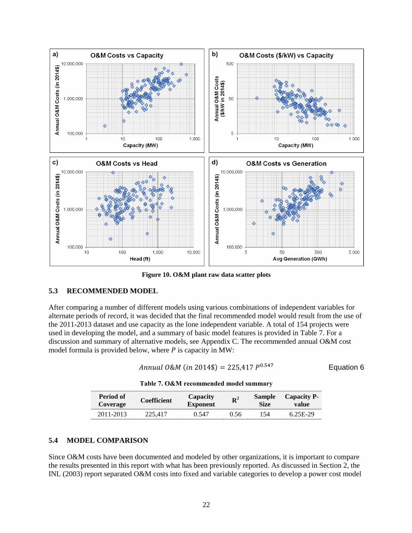
22

Figure 10. O&M plant raw data scatter plots

5.3 RECOMMENDED MODEL

After comparing a number of different models using various combinations of independent variables for

alternate periods of record, it was decided that the final recommended model would result from the use of

the 2011-2013 dataset and use capacity as the lone independent variable. A total of 154 projects were

used in developing the model, and a summary of basic model features is provided in Table 7. For a

discussion and summary of alternative models, see Appendix C. The recommended annual O&M cost

model formula is provided below, where 𝑃 is capacity in MW:

𝐴𝑛𝑛𝑢𝑎𝑙 𝑂&𝑀 (𝑖𝑛 2014$) = 225,417 𝑃0.547 Equation 6

Table 7. O&M recommended model summary

Period of

Coverage Coefficient

Capacity

Exponent R

2

Sample

Size

Capacity P-

value

2011-2013 225,417 0.547 0.56 154 6.25E-29

5.4 MODEL COMPARISON

Since O&M costs have been documented and modeled by other organizations, it is important to compare

the results presented in this report with what has been previously reported. As discussed in Section 2, the

INL (2003) report separated O&M costs into fixed and variable categories to develop a power cost model

23

based on plant capacity. After combining the fixed and variable cost estimates and escalating to 2014$, a

direct comparison between the INL and ORNL models could be made.

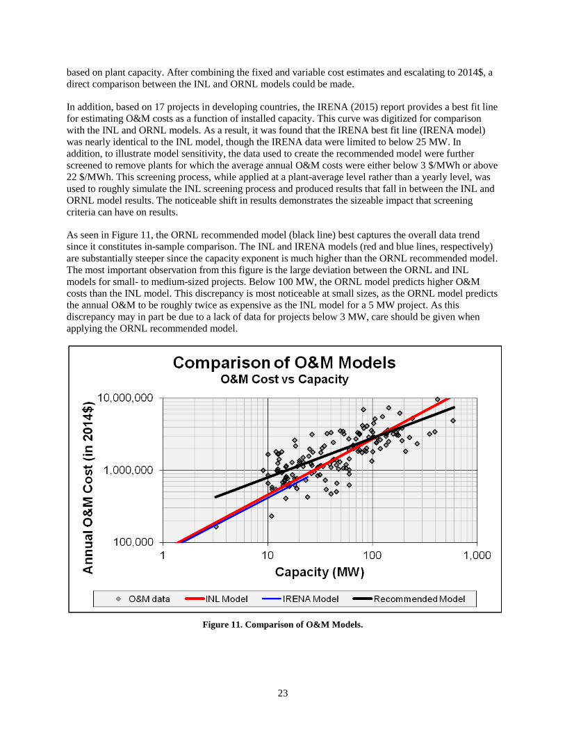
In addition, based on 17 projects in developing countries, the IRENA (2015) report provides a best fit line

for estimating O&M costs as a function of installed capacity. This curve was digitized for comparison

with the INL and ORNL models. As a result, it was found that the IRENA best fit line (IRENA model)

was nearly identical to the INL model, though the IRENA data were limited to below 25 MW. In

addition, to illustrate model sensitivity, the data used to create the recommended model were further

screened to remove plants for which the average annual O&M costs were either below 3 $/MWh or above

22 $/MWh. This screening process, while applied at a plant-average level rather than a yearly level, was

used to roughly simulate the INL screening process and produced results that fall in between the INL and

ORNL model results. The noticeable shift in results demonstrates the sizeable impact that screening

criteria can have on results.

As seen in Figure 11, the ORNL recommended model (black line) best captures the overall data trend

since it constitutes in-sample comparison. The INL and IRENA models (red and blue lines, respectively)

are substantially steeper since the capacity exponent is much higher than the ORNL recommended model.

The most important observation from this figure is the large deviation between the ORNL and INL

models for small- to medium-sized projects. Below 100 MW, the ORNL model predicts higher O&M

costs than the INL model. This discrepancy is most noticeable at small sizes, as the ORNL model predicts

the annual O&M to be roughly twice as expensive as the INL model for a 5 MW project. As this

discrepancy may in part be due to a lack of data for projects below 3 MW, care should be given when

applying the ORNL recommended model.

Figure 11. Comparison of O&M Models.

24

5.5 MODEL APPLICATION

Based on the data used to develop the recommended O&M cost model, Equation 6 should ideally be

applied for projects with a total capacity between 3 and 600 MW. Due to this data limitation, which most

notably excludes projects below 3 MW, an alternative costing method for estimating O&M costs for

small- to medium-sized projects was desired.

As reported in the IRENA report, annual O&M costs are often represented as a percentage of ICC.

Typically, annual O&M costs range from 1-4% of ICC, and the International Energy Agency assumes

2.2% for large and 2.2% to 3% for small hydropower projects (IRENA, 2015). Data on individual projects

from IRENA (2014) range from 0.1 to 24 MW, with an annual O&M cost ranging from 0.6% to 6.1% of

ICC.

In light of the potential for overestimation, it is recommended that the lesser of 1) the ORNL

recommended model (Equation 6) or a rough approximation of 2.5% of ICC be used.

Since both ICC and O&M data have been collected as a part of this BCM report, direct comparison

between actual and predicted O&M costs can be made for any recently developed projects for which

O&M data are available. When identifying data to be used for comparison, capacity additions at existing

hydropower facilities could not be directly used, as the Form 1 O&M data does not distinguish between

generating units. Thus, only plants for which total installed capacity matched between the ICC and O&M

databases could be used. Among the data available, only 3 plants are common to the ICC and O&M

databases and could be used for comparison. The average annual O&M cost was determined for each

project based on the period of coverage available.

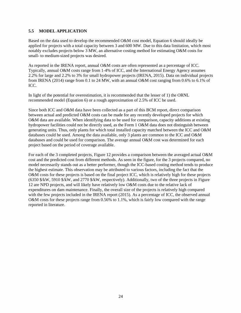
For each of the 3 completed projects, Figure 12 provides a comparison between the averaged actual O&M

cost and the predicted cost from different methods. As seen in the figure, for the 3 projects compared, no

model necessarily stands out as a better performer, though the ICC-based costing method tends to produce

the highest estimate. This observation may be attributed to various factors, including the fact that the

O&M costs for these projects is based on the final project ICC, which is relatively high for these projects

(6350 $/kW, 5910 $/kW, and 2770 $/kW, respectively). Additionally, two of the three projects in Figure

12 are NPD projects, and will likely have relatively low O&M costs due to the relative lack of

expenditures on dam maintenance. Finally, the overall size of the projects is relatively high compared

with the few projects included in the IRENA report (2015). As a percentage of ICC, the observed annual

O&M costs for these projects range from 0.56% to 1.1%, which is fairly low compared with the range

reported in literature.

25

Figure 12. Comparison of annual O&M costs for ORNL completed projects.

5.6 CONSIDERATIONS FOR MODEL APPLICATION

Based on the data used to develop the recommended O&M cost model, Equation 6 should only be applied

for projects with a total capacity between 3 and 600 MW, though it is recommended that the lesser of

Equations 6 and 7 be used. While the recommended model does not produce the highest R2 value, and the

introduction of a longer period of coverage or more variables would increase the statistical performance,

it was decided that this model captured the primary cost driver without adding additional complexity that

may not truly improve the model’s predictive capability. The shortened period of coverage, while

providing only a snapshot of the data collected, was selected since it represents recent O&M costs and

reduces potential bias from older data for which cost escalation may not fully capture the increases in

O&M. The 1994-2013 dataset’s capacity-only model produces costs that are roughly 10% lower than the

recommended model. Additionally, when evaluated using different periods of coverage, the capacity-only

models produced nearly the exact same capacity exponent, indicating that the underlying relationship

between O&M cost and capacity is not influenced by the dataset used to model. Thus, in order to maintain

conservatism and better represent the recent, higher O&M costs, the 2011-2013 dataset was

recommended.

In addition, the regression results when including head, generation, and regional variables did not

convince staff that inclusion of these variables would be appropriate. When evaluating head, the positive

exponent was unexpected, running counter to engineering knowledge. Also, the relatively small exponent

and variation in magnitude across different datasets suggested the effect was unlikely to be statistically

genuine. For generation, while results were relatively consistent across datasets and were statistically

significant, it was felt that the addition of this secondary variable did not provide enough benefit to be

included in the recommended model. The use of regional dummy variables resulted in slightly higher R2

values; however, the additional regional adjustment fails to noticeably improve individual plant

estimation, instead only providing an approximation of the average regional cost level. Furthermore, due

26

to data limitations, some regions of the U.S. are not well represented, so the dummy variables tend to be

heavily biased for particular regions. In the end, only capacity was retained for the final recommended

model. Additional details on the development of alternative O&M models are provided in Appendix C.

6. CONTEMPORARY HYDROPOWER DEVELOPMENT AND APPLICATION TO U.S.

HYDROPOWER RESOURCE ASSESSMENTS

The primary goal of these hydropower cost models is to provide “average” cost estimation for

undeveloped hydropower applications. Ultimately, these models cannot capture the site specific

characteristics which influence project management and design; however, they may provide a high level

cost evaluation useful in preliminary feasibility assessment. When applied at a national scale, these

models can demonstrate the level of feasibility and competitiveness associated with undeveloped

hydropower resources in the U.S. Before applying the cost models to the previously developed resource

assessments, it is important to understand the cost distributions experienced in recent development.

6.1 LCOE DISTRIBUTIONS FOR RECENT DEVELOPMENT

Levelized cost of energy (LCOE) is an additional metric by which to evaluate the economics of

hydropower resources. In order to estimate LCOE, plant-specific generation estimates for U.S. projects

were collected alongside capital costs. Annual O&M costs were estimated by using the lesser of the

recommended model or 2.5% of ICC, as described in Section 5. Licensing costs were estimated using

escalated cost equations from Idaho National Laboratory (INL, 2003), as provided in the Section 4.

Licensing costs for Canal/Conduit projects were estimated using the NPD equation. One key aspect of

the licensing process that makes it large cost component is the fact that project development and licensing

costs are typically accrued many years before a project reaches commercial operation—of plants placed in

service over the last decade, the average FERC-licensing hydropower project has taken 5 years from

initial permit application to construction start (Uria-Martinez et. al., 2015). To better simulate the present

value of incurring these costs, it is assumed that expenditures are evenly split across the five years,

resulting in present value cost increase of 20% (this assumes a 6.2% discount rate as discussed later).

As can be seen in Figure 13, the LCOE of recent development for all three resource classes is generally

similar. The median LCOE for each class is approximately 120 $/MWh and generally exhibits less

variation than ICC alone. This convergence is driven by two factors: (1) only economically competitive

projects will be developed and constructed; therefore, high ICC projects require higher capacity factors

for competitive LCOE—and (2) accordingly, NSD and NPD projects have higher capacity factors than

Canal/Conduit projects. Projects constructed on existing water supply infrastructure, such as

Canal/Conduits, are only able to produce power when flows are scheduled to meet water demands and

may operate on a seasonal basis and thus typically have a lower capacity factor.

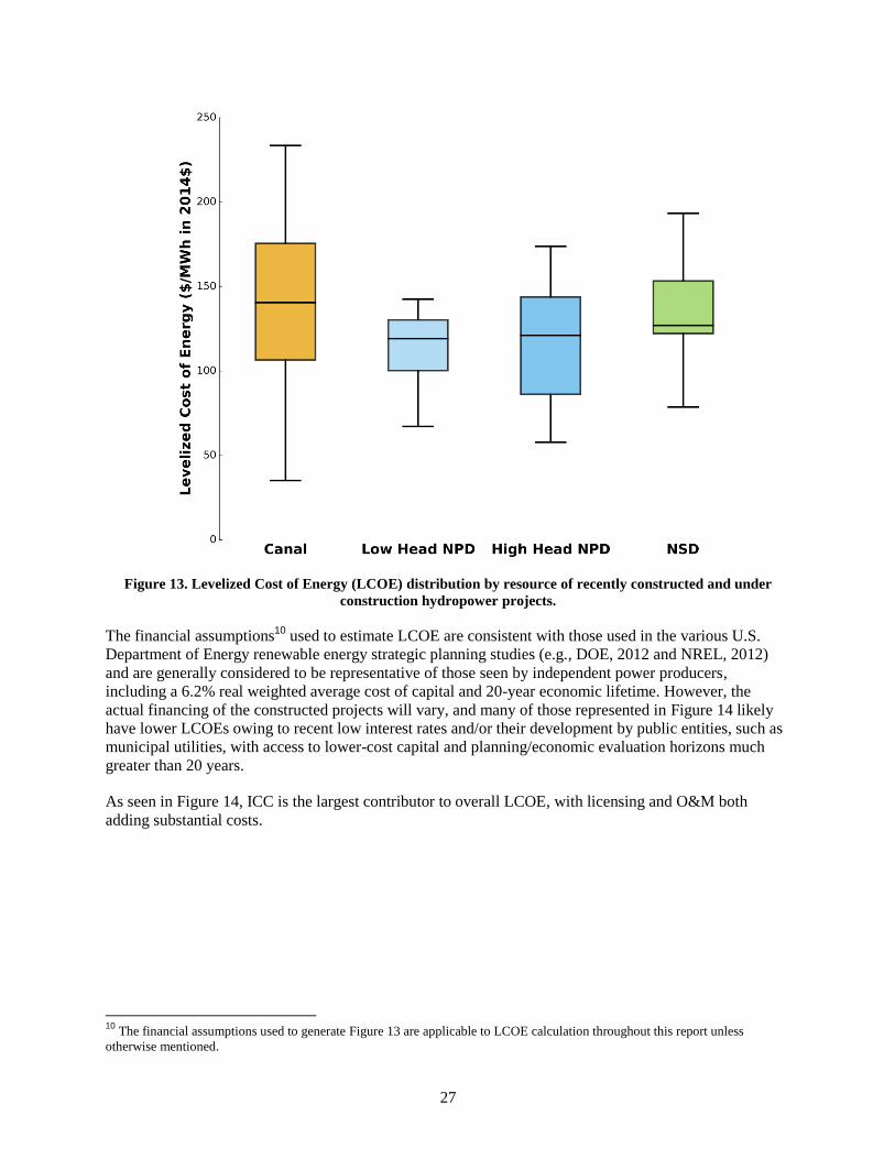
27

Figure 13. Levelized Cost of Energy (LCOE) distribution by resource of recently constructed and under


The financial assumptions10

used to estimate LCOE are consistent with those used in the various U.S.

Department of Energy renewable energy strategic planning studies (e.g., DOE, 2012 and NREL, 2012)

and are generally considered to be representative of those seen by independent power producers,

including a 6.2% real weighted average cost of capital and 20-year economic lifetime. However, the

actual financing of the constructed projects will vary, and many of those represented in Figure 14 likely

have lower LCOEs owing to recent low interest rates and/or their development by public entities, such as

municipal utilities, with access to lower-cost capital and planning/economic evaluation horizons much

greater than 20 years.

As seen in Figure 14, ICC is the largest contributor to overall LCOE, with licensing and O&M both

adding substantial costs.

10

The financial assumptions used to generate Figure 13 are applicable to LCOE calculation throughout this report unless

otherwise mentioned.

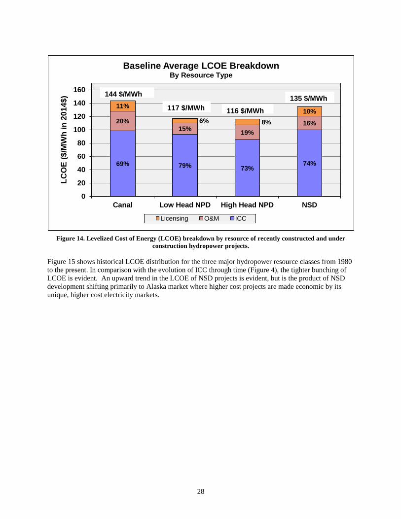
28

Figure 14. Levelized Cost of Energy (LCOE) breakdown by resource of recently constructed and under


Figure 15 shows historical LCOE distribution for the three major hydropower resource classes from 1980

to the present. In comparison with the evolution of ICC through time (Figure 4), the tighter bunching of

LCOE is evident. An upward trend in the LCOE of NSD projects is evident, but is the product of NSD

development shifting primarily to Alaska market where higher cost projects are made economic by its

unique, higher cost electricity markets.

69% 79% 73% 74%

20%

15% 19%

16%

11%

6% 8%

10%

0

20

40

60

80

100

120

140

160

Canal Low Head NPD High Head NPD NSD

LC

OE

($/M

Wh

in

20

14

$)

Baseline Average LCOE Breakdown By Resource Type

Licensing O&M ICC

117 $/MWh 116 $/MWh

144 $/MWh 135 $/MWh

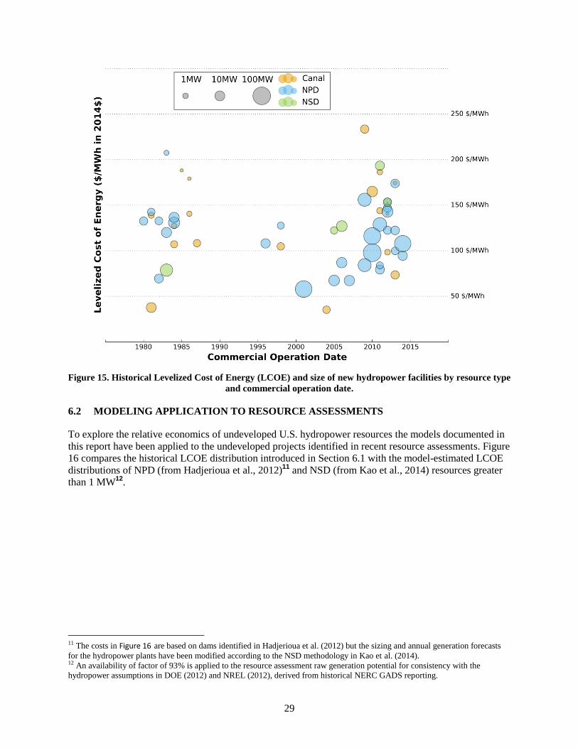
29

Figure 15. Historical Levelized Cost of Energy (LCOE) and size of new hydropower facilities by resource type

and commercial operation date.

6.2 MODELING APPLICATION TO RESOURCE ASSESSMENTS

To explore the relative economics of undeveloped U.S. hydropower resources the models documented in

this report have been applied to the undeveloped projects identified in recent resource assessments. Figure

16 compares the historical LCOE distribution introduced in Section 6.1 with the model-estimated LCOE

distributions of NPD (from Hadjerioua et al., 2012)11

and NSD (from Kao et al., 2014) resources greater

than 1 MW12

.

11 The costs in Figure 16 are based on dams identified in Hadjerioua et al. (2012) but the sizing and annual generation forecasts

for the hydropower plants have been modified according to the NSD methodology in Kao et al. (2014). 12 An availability of factor of 93% is applied to the resource assessment raw generation potential for consistency with the

hydropower assumptions in DOE (2012) and NREL (2012), derived from historical NERC GADS reporting.

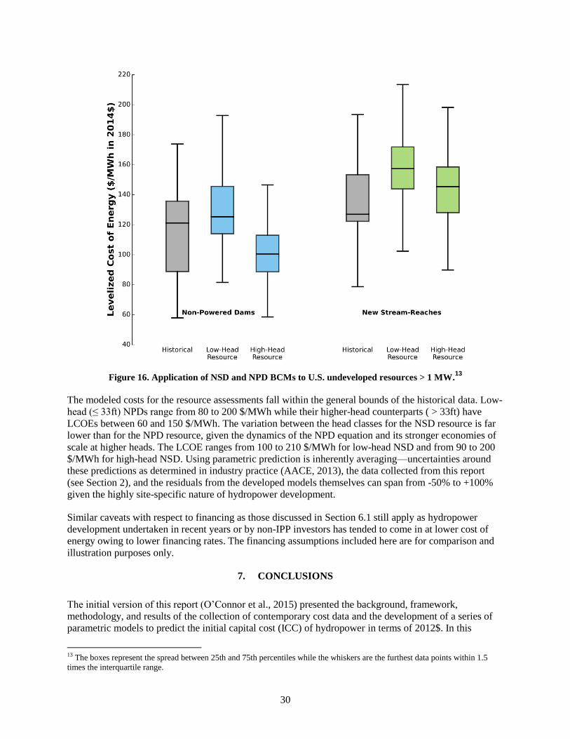
30

Figure 16. Application of NSD and NPD BCMs to U.S. undeveloped resources > 1 MW.13

The modeled costs for the resource assessments fall within the general bounds of the historical data. Low-

head (≤ 33ft) NPDs range from 80 to 200 $/MWh while their higher-head counterparts ( > 33ft) have

LCOEs between 60 and 150 $/MWh. The variation between the head classes for the NSD resource is far

lower than for the NPD resource, given the dynamics of the NPD equation and its stronger economies of

scale at higher heads. The LCOE ranges from 100 to 210 $/MWh for low-head NSD and from 90 to 200

$/MWh for high-head NSD. Using parametric prediction is inherently averaging—uncertainties around

these predictions as determined in industry practice (AACE, 2013), the data collected from this report

(see Section 2), and the residuals from the developed models themselves can span from -50% to +100%

given the highly site-specific nature of hydropower development.

Similar caveats with respect to financing as those discussed in Section 6.1 still apply as hydropower

development undertaken in recent years or by non-IPP investors has tended to come in at lower cost of

energy owing to lower financing rates. The financing assumptions included here are for comparison and

illustration purposes only.

7. CONCLUSIONS

The initial version of this report (O’Connor et al., 2015) presented the background, framework,

methodology, and results of the collection of contemporary cost data and the development of a series of

parametric models to predict the initial capital cost (ICC) of hydropower in terms of 2012$. In this

13 The boxes represent the spread between 25th and 75th percentiles while the whiskers are the furthest data points within 1.5

times the interquartile range.

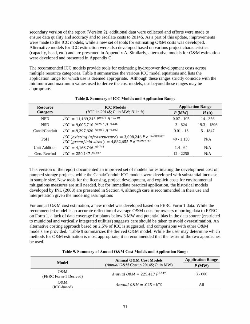
31

secondary version of the report (Version 2), additional data were collected and efforts were made to

ensure data quality and accuracy and to escalate costs to 2014$. As a part of this update, improvements

were made to the ICC models, while a new set of tools for estimating O&M costs was developed.

Alternative models for ICC estimation were also developed based on various project characteristics

(capacity, head, etc.) and are presented in Appendix A. Similarly, alternative models for O&M estimation

were developed and presented in Appendix C.

The recommended ICC models provide tools for estimating hydropower development costs across

multiple resource categories. Table 8 summarizes the various ICC model equations and lists the

application range for which use is deemed appropriate. Although these ranges strictly coincide with the

minimum and maximum values used to derive the cost models, use beyond these ranges may be

appropriate.

Table 8. Summary of ICC Models and Application Range

Resource

Category

ICC Models

(ICC in 2014$; P in MW; H in ft)

Application Range

P (MW) H (ft)

NPD 𝐼𝐶𝐶 = 11,489,245 𝑃0.976 𝐻−0.240 0.07 - 105 14 - 356

NSD 𝐼𝐶𝐶 = 9,605,710 𝑃0.977 𝐻−0.126 3 - 824 19.3 – 1896

Canal/Conduit 𝐼𝐶𝐶 = 9,297,820 𝑃0.810 𝐻−0.102 0.01 - 13 5 - 1847

PSH 𝐼𝐶𝐶 (𝑒𝑥𝑖𝑠𝑡𝑖𝑛𝑔 𝑖𝑛𝑓𝑟𝑎𝑠𝑡𝑟𝑢𝑐𝑡𝑢𝑟𝑒) = 3,008,246 𝑃 𝑒−0.000460𝑃

𝐼𝐶𝐶 (𝑔𝑟𝑒𝑒𝑛𝑓𝑖𝑒𝑙𝑑 𝑠𝑖𝑡𝑒𝑠 ) = 4,882,655 𝑃 𝑒−0.000776𝑃 40 - 1,150 N/A

Unit Addition 𝐼𝐶𝐶 = 4,163,746 𝑃0.741 1.4 - 64 N/A

Gen. Rewind 𝐼𝐶𝐶 = 250,147 𝑃0.817 12 - 2250 N/A

This version of the report documented an improved set of models for estimating the development cost of

pumped storage projects, while the Canal/Conduit ICC models were developed with substantial increase

in sample size. New tools for the licensing, project development, and explicit costs for environmental

mitigations measures are still needed, but for immediate practical application, the historical models

developed by INL (2003) are presented in Section 4, although care is recommended in their use and

interpretation given the modeling assumptions

For annual O&M cost estimation, a new model was developed based on FERC Form 1 data. While the

recommended model is an accurate reflection of average O&M costs for owners reporting data to FERC

on Form 1, a lack of data coverage for plants below 3 MW and potential bias in the data source (restricted

to municipal and vertically integrated utilities) suggests care should be taken to avoid overestimation. An

alternative costing approach based on 2.5% of ICC is suggested, and comparisons with other O&M

models are provided. Table 9 summarizes the derived O&M model. While the user may determine which

methods for O&M estimation is most appropriate, it is recommended that the lesser of the two approaches

be used.

Table 9. Summary of Annual O&M Cost Models and Application Range

Model Annual O&M Cost Models

(Annual O&M Cost in 2014$; P in MW)

Application Range

P (MW)

O&M

(FERC Form-1 Derived) 𝐴𝑛𝑛𝑢𝑎𝑙 𝑂&𝑀 = 225,417 𝑃0.547 3 - 600

O&M

(ICC-based) 𝐴𝑛𝑛𝑢𝑎𝑙 𝑂&𝑀 = .025 ∗ 𝐼𝐶𝐶 All

32

For all of the models presented, consideration should be paid to limitations related to raw data breadth,

and attempts have been made to identify such limitations. As this report is intended to be a living

document, changes may be made to the recommended cost models based upon future improvements. With

the addition of more diverse data and advanced validation, future model iterations should provide

improved results.

8. REFERENCES

AACE (2013). Cost Estimate Classification System – As Applied in Engineering, Procurement, and

Construction for the Hydropower Industry. AACE International Recommended Practice No. 69R-12.

January, 2013.

Butterfield, S. (2011). Presentation on Swalley Irrigation District’s Ponderosa Hydroelectric Project

during the Deschutes River Basin Site Visit. Swalley Irrigation District, June 1, 2011.

City of Boulder (2013), City of Boulder Hydroelectric Facility Summary Sheet, available at https://www-

static.bouldercolorado.gov/docs/Agenda_5_-_Hydroelectric_Program_Update-1-201307111316.pdf,

accessed online March 2014.

COID (Central Oregon Irrigation District) and ODE (Oregon Department of Energy) (2011). Feasibility

Study for Six Central Oregon Irrigation District Potential Hydroelectric Power Generation Sites,

Oregon.

DOE (Department of Energy) and, EPRI (Electric Power Research Institute) (1985a). Small-Hydropower

Development: The Process, Pitfalls, and Experience Volume 1: Feasibility Studies Summary and

Analysis, EPRI EM-4036.

DOE (Department of Energy) and EPRI (Electric Power Research Institute) (1985b). Small-Hydropower

Development: The Process, Pitfalls, and Experience Volume 2: Licensing Activities Summary and

Analysis, EPRI EM-4036.

DOE (Department of Energy) and EPRI (Electric Power Research Institute) (1986). Small-Hydropower

Development: The Process, Pitfalls, and Experience Volume 4: Guide for Developers, EPRI EM-

4036.

DOE (Department of Energy) and, EPRI (Electric Power Research Institute) (1987). Small-Hydropower

Development: The Process, Pitfalls, and Experience Volume 3: Summary and Analysis of

Technology Development Projects, EPRI EM-4036.

DOE (Department of Energy) (2014). Presentation on Recovery Act: Hydroelectric Facility

Modernization Project, accessed on February, 2014.

DOE (Department of Energy) (2015). Wind Vision: A New Era for Wind Power in the United States,

DOE/GO-102015-4557

EIA (Energy Information Administration) (2013). Updated Capital Cost Estimates for Utility Scale

Electricity Generating Plants, available at

http://www.eia.gov/forecasts/capitalcost/pdf/updated_capcost.pdf, accessed online January 2014.

EIA (Energy Information Administration) (2014). Annual Energy Outlook 2014: with Projections to

2040, DOE/EIA-0383(2014). Washington, DC.

ENR (Engineering News Record) (2013). Construction Cost Indices, Engineering News Record, available

online at http://enr.construction.com/economics/, accessed online June 2013.

EPRI (2011) Quantifying the Value of Hydropower in the Electric Grid: Plant Cost Elements. EPRI, Palo

Alto, CA: 2011. 1023140.

https://www-static.bouldercolorado.gov/docs/Agenda_5_-_Hydroelectric_Program_Update-1-201307111316.pdf

https://www-static.bouldercolorado.gov/docs/Agenda_5_-_Hydroelectric_Program_Update-1-201307111316.pdf

http://www.eia.gov/forecasts/capitalcost/pdf/updated_capcost.pdf

http://enr.construction.com/economics/

33

ETO (Energy Trust of Oregon) (2010). Irrigation Water Providers of Oregon: Hydropower Potential and

Energy Savings Evaluation, Oregon.

FERC (Federal Energy Regulatory Commission) (2014). Federal Energy Regulatory Commission,

available at http://www.ferc.gov/, accessed online January 2014.

FERC (Federal Energy Regulatory Commission) (2015). Federal Energy Regulatory Commission Form 1

data, available at http://www.ferc.gov/, accessed online January 2015.

Figueiredo, F.C. and Flynn. P.C. (2006). "Using Diurnal Power price to Configure Pumped Storage",

IEEE Transactions on Energy Conversion, Vol. 21, No.3

Hadjerioua, B., Wei, Y., and Kao, S.C. (2012). An Assessment of Energy Potential at Non-powered Dams

in the United States, GPO DOE/EE-0711, Wind and Water Power Program, Department of Energy,

DC.

IIR (Industrial Info Resources) (2014). PECWeb – A Searchable Database, available at

http://www.industrialinfo.com/database , accessed online March 2014.

INL (Idaho National Lab) (2003). Estimation of Economic Parameters of U.S. Hydropower Resources,

INEEL/EXT-03-00662.

IRENA (International Renewable Energy Agency) (2015). Renewable Power Generation Costs in 2014,

Innovation and Technology Centre, Bonn Germany

Kao, S.C., McManamay, R.A., Stewart, K.M., Samu, N.M., Hadjerioua, B., DeNeale, S.T., Yeasmin, D.,

Pasha, M.F. K., Oubeidillah, A.A., and Smith, B.T. (2014). New Stream-reach Development: A

Comprehensive Assessment of Hydropower Energy Potential in the United States, GPO DOE/EE-

1063, Wind and Water Power Program, Department of Energy, Washington, DC.

NHAAP (National Hydropower Asset Assessment Program) (2015). Oak Ridge National Laboratory,

available at http://nhaap.ornl.gov/, accessed online March 2015.

NREL (National Renewable Energy Laboratory) (2012). Renewable Electricity Futures Study, 4 vols.

NREL/TP-6A20-52409, Golden, Colorado.

NUID (North Unit Irrigation District) (2009). Feasibility Study on Five Potential Hydroelectric Power

Generation Locations in the North Unit Irrigation District, Oregon, August 2009.

O’Connor, P.W., Zhang, Q.F., DeNeale, S.T., Chalise, D.R., Centurion, E (2015) “Hydropower Baseline

Cost Modeling”, ORNL/TM 2014/15.

OpenEI (Open Energy Forum) (2014). Transparent Cost Database, available at

http://en.openei.org/wiki/Transparent_Cost_Database, accessed online August 2014.

RSMeans (2013). Historical Cost Indices, RSMeans, available online at http://www.rsmeansonline.com,

accessed online June 2013.

TVA (Tennessee Valley Authority) (1941). The Guntersville Project: A Comprehensive Report on the

Planning, Design, Construction, and Initial Operations of the Guntersville Project, Technical Report

No. 4, Knoxville, Tennessee.

USACE (United States Army Corps of Engineers) and MWH (2009). Technical Analysis of Pumped

Storage and Integration with Wind Power in the Pacific Northwest. MWH Prepared for U.S. Army

Corps of Engineers, Northwest Division, Hydroelectric Design Center.

USACE (United States Army Corps of Engineers) (2013). Hydropower Resource Assessment At Non-

Powered USACE Sites.

http://www.ferc.gov/

http://www.ferc.gov/

http://www.industrialinfo.com/database

http://nhaap.ornl.gov/

http://en.openei.org/wiki/Transparent_Cost_Database

http://www.rsmeansonline.com/

34

USBR (United States Bureau of Reclamation) (1988). Spring Canyon Pumped Storage Project, Bureau of

Reclamation, Lower Colorado Region, Boulder City, Nevada, October 1988.

USBR (United States Bureau of Reclamation) (2015). Hydropower Construction Costs Trends, Bureau of

Reclamation, available online at http://www.usbr.gov/pmts/estimate/cost_trend.html, accessed online

January 2015.

Uria-Martinez, R.; P.W. O’Connor, P. W.; M.M. Johnson (2015). 2014 Hydropower Market Report. GPO

DOE/EE-1195. Washington, DC: Wind and Water Power Technologies Office, U.S. Department of

Energy.

Zhang, Q.F., Smith, B., and Zhang, W. (2012). Small Hydropower Cost Reference Model, ORNL/TM-

2012/501.

http://www.usbr.gov/pmts/estimate/cost_trend.html

APPENDIX A. ICC DATA SOURCES, ALTERNATIVE MODELS, AND

VALIDATION

A-3

APPENDIX A. ICC DATA SOURCES, ALTERNATIVE MODELS, AND VALIDATION

Raw Data

Section 4 provides summary data statistics for each resource class without providing details on data

sources. Since there is no discussion on raw data that illustrates the primary data sources, tables have been

provided to demonstrate data statistics including project counts, as well as minimum, average, and

maximum capacity and head values for each data source. Table A.1-Table A.6 provides data statistics for

each resource type by data source. Figure A.1 shows statistical distribution of cost data, providing the

number of projects in each resource category, along with the average ICC. As shown in Figure A.1, NSD,

NPD, and Canal/Conduit projects tend to have the highest per kW development costs, while the plant

overhaul-related projects tend to have a much lower cost. As the plot is shown on a logarithmic scale, the

magnitude of cost variation is somewhat skewed. In Figure A.1, one can see that certain types of projects

(NPDs for instance) contain relatively high variability, while others (such as Unit Addition) are relatively

consistent in terms of cost.

A total of 680 projects were used for the final analysis. 653 out of 680 projects were located in the U.S.

with the remaining 27 projects from Non-US regions. As shown in Figure A.2, the United States was

divided into six market regions: Southwest, Midwest, Rocky Mountains, Pacific, Southeast, and

Northeast.

For each of the resource categories, Appendix A provides information on regional cost data distributions,

raw data histogram-scatter plots, alternative models, and in-sample model validation. The regional raw

cost data distribution diagram provides statistics on the U.S. (six regions) and Non-US data. However, the

discussion on raw cost data are focused on the U.S. regions only. Alternative models which were

developed based on project development stage, installed capacity and hydraulic head ranges are

documented. The raw costs vs. model estimated costs are compared using in-sample validation plots.

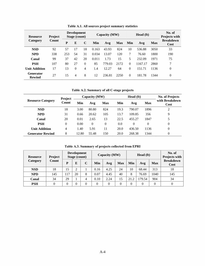
A-4

Table A.1. All sources project summary statistics

Resource

Category

Project

Count

Development

Stage (count) Capacity (MW) Head (ft)

No. of

Projects with

Breakdown


NSD 92 57 17 18 0.163 43.93 824 10 536.88 3050 33

NPD 338 253 54 31 0.034 13.07 120 7 76.60 1800 190

Canal 99 37 42 20 0.011 1.73 15 5 232.09 1971 75

PSH 107 80 27 0 85 779.03 2172 0 1167.17 2860 7

Unit Addition 17 13 0 4 1.4 12.27 64 0 151.71 1136 0

Generator

Rewind 27 15 4 8 12 236.81 2250 0 181.78 1344 0

Table A.2. Summary of all C-stage projects

Resource Category Project

Count

Capacity (MW) Head (ft) No. of Projects

with Breakdown

Cost Min Avg Max Min Avg Max

NSD 18 3.00 80.80 824 19.3 790.07 1896 2

NPD 31 0.66 20.62 105 13.7 109.85 356 9

Canal 20 0.01 2.65 13 22.5 455.27 1847 5

PSH 0 0.00 0 0 0.0 0 0 0

Unit Addition 4 1.40 5.91 11 20.0 436.50 1136 0

Generator Rewind 8 12.80 55.48 150 20.0 268.38 1344 0

Table A.3. Summary of projects collected from EPRI

Resource

Category

Project

Count

Development


No. of

Projects with

Breakdown


NSD 18 15 2 1 0.16 4.25 24 10 68.44 313 18

NPD 145 117 20 8 0.07 4.45 40 8 76.69 1040 145

Canal 34 29 1 4 0.10 2.24 15 21.2 179.54 904 34

PSH 0 0 0 0 0 0 0 0 0 0 0

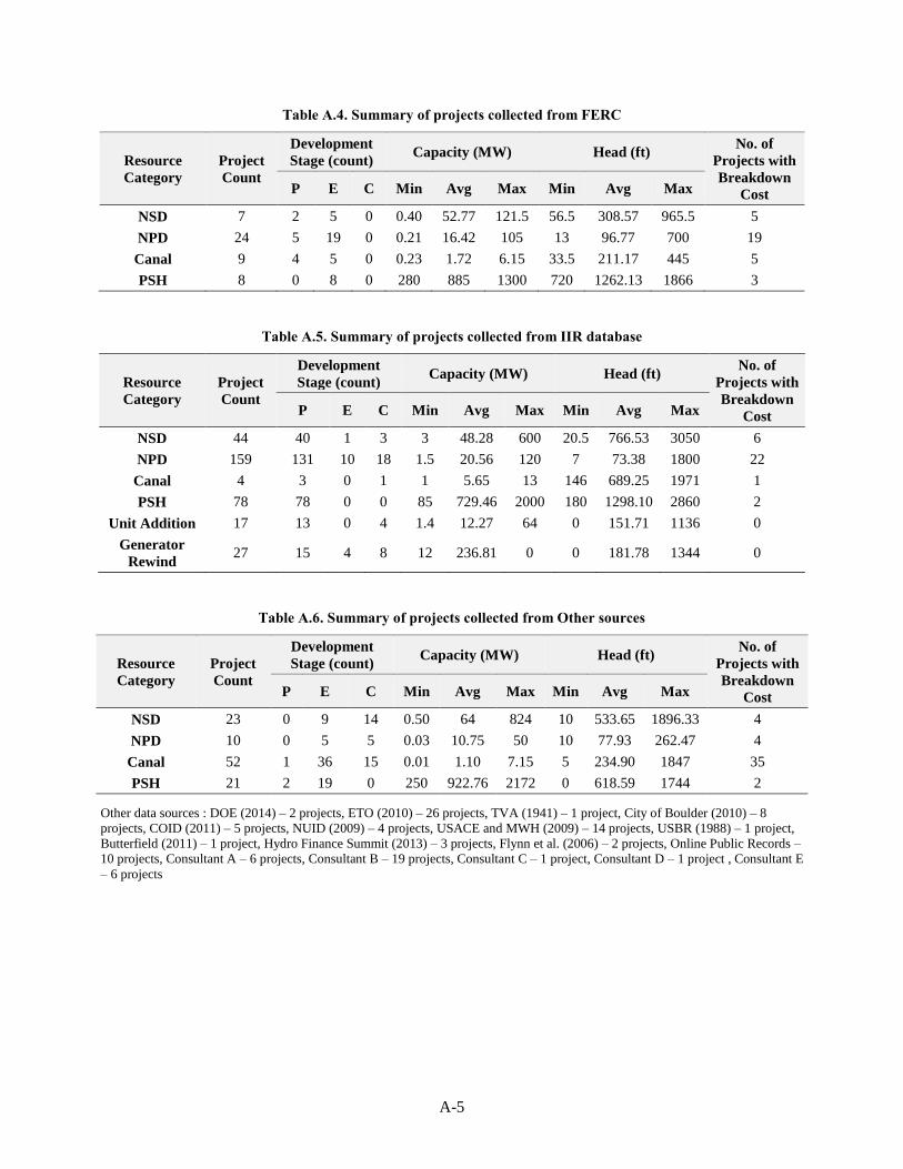
A-5

Table A.4. Summary of projects collected from FERC

Resource

Category

Project

Count

Development


No. of

Projects with

Breakdown


NSD 7 2 5 0 0.40 52.77 121.5 56.5 308.57 965.5 5

NPD 24 5 19 0 0.21 16.42 105 13 96.77 700 19

Canal 9 4 5 0 0.23 1.72 6.15 33.5 211.17 445 5

PSH 8 0 8 0 280 885 1300 720 1262.13 1866 3

Table A.5. Summary of projects collected from IIR database

Resource

Category

Project

Count

Development


No. of

Projects with

Breakdown


NSD 44 40 1 3 3 48.28 600 20.5 766.53 3050 6

NPD 159 131 10 18 1.5 20.56 120 7 73.38 1800 22

Canal 4 3 0 1 1 5.65 13 146 689.25 1971 1

PSH 78 78 0 0 85 729.46 2000 180 1298.10 2860 2

Unit Addition 17 13 0 4 1.4 12.27 64 0 151.71 1136 0

Generator

Rewind 27 15 4 8 12 236.81 0 0 181.78 1344 0

Table A.6. Summary of projects collected from Other sources

Resource

Category

Project

Count

Development


No. of

Projects with

Breakdown


NSD 23 0 9 14 0.50 64 824 10 533.65 1896.33 4

NPD 10 0 5 5 0.03 10.75 50 10 77.93 262.47 4

Canal 52 1 36 15 0.01 1.10 7.15 5 234.90 1847 35

PSH 21 2 19 0 250 922.76 2172 0 618.59 1744 2

Other data sources : DOE (2014) – 2 projects, ETO (2010) – 26 projects, TVA (1941) – 1 project, City of Boulder (2010) – 8

projects, COID (2011) – 5 projects, NUID (2009) – 4 projects, USACE and MWH (2009) – 14 projects, USBR (1988) – 1 project,

Butterfield (2011) – 1 project, Hydro Finance Summit (2013) – 3 projects, Flynn et al. (2006) – 2 projects, Online Public Records –

10 projects, Consultant A – 6 projects, Consultant B – 19 projects, Consultant C – 1 project, Consultant D – 1 project , Consultant E

– 6 projects

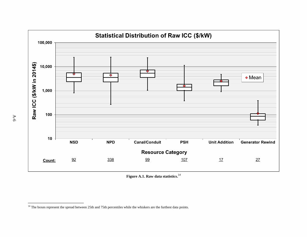
A-6

Figure A.1. Raw data statistics.14

14 The boxes represent the spread between 25th and 75th percentiles while the whiskers are the furthest data points.

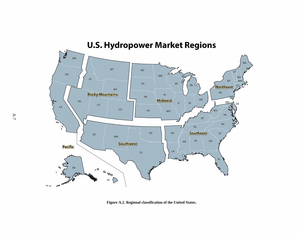
A-7

Figure A.2. Regional classification of the United States.

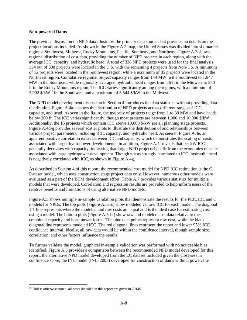
A-8

Non-powered Dams

The previous discussion on NPD data illustrates the primary data sources but provides no details on the

project locations included. As shown in the Figure A.2 map, the United States was divided into six market

regions: Southwest, Midwest, Rocky Mountains, Pacific, Southeast, and Northeast. Figure A.3 shows

regional distribution of cost data, providing the number of NPD projects in each region, along with the

average ICC, capacity, and hydraulic head. A total of 338 NPD projects were used for the final analysis.

334 out of 338 projects were located in the U.S. with the remaining 4 projects from Non-US. A minimum

of 12 projects were located in the Southwest region, while a maximum of 85 projects were located in the

Northeast region. Cumulative regional project capacity ranges from 144 MW in the Southwest to 1,847

MW in the Southeast, while regionally-averaged hydraulic head ranges from 26 ft in the Midwest to 250

ft in the Rocky Mountains region. The ICC varies significantly among the regions, with a minimum of

2,902 $/kW15

in the Southwest and a maximum of 5,544 $/kW in the Midwest.

The NPD model development discussion in Section 4 introduces the data statistics without providing data

distribution. Figure A.4a-c shows the distribution of NPD projects across different ranges of ICC,

capacity, and head. As seen in the figure, the majority of projects range from 1 to 30 MW and have heads

below 200 ft. The ICC varies significantly, though most projects are between 1,000 and 10,000 $/kW1.

Additionally, the 16 projects which contain ICC above 10,000 $/kW are all planning stage projects.

Figure A.4d-g provides several scatter plots to illustrate the distribution of and relationships between

various project parameters, including ICC, capacity, and hydraulic head. As seen in Figure A.4e, an

apparent positive correlation exists between ICC and capacity, which demonstrates the scaling of costs

associated with larger hydropower developments. In addition, Figure A.4f reveals that per kW ICC

generally decreases with capacity, indicating that larger NPD projects benefit from the economies of scale

associated with large hydropower development. Though not as strongly correlated to ICC, hydraulic head

is negatively correlated with ICC, as shown in Figure A.4g.

As described in Section 4 of this report, the recommended cost model for NPD ICC estimation is the C

Dataset model, which uses construction stage project data only. However, numerous other models were

evaluated as a part of the BCM development effort. Table A.7 provides various statistics for multiple

models that were developed. Correlation and regression results are provided to help inform users of the

relative benefits and limitations of using alternative NPD models.

Figure A.5 shows multiple in-sample validation plots that demonstrate the results for the PEC, EC, and C

models for NPDs. The top plots (Figure A.5a-c) show modeled vs. raw ICC for each model. The diagonal

1:1 line represents where the modeled and raw costs are equal and is the ideal case for estimating cost

using a model. The bottom plots (Figure A.5d-f) show raw and modeled cost data relative to the

combined capacity and head power forms. The blue data points represent raw cost, while the black

diagonal line represents modeled ICC. The red diagonal lines represent the upper and lower 95% ICC

confidence interval. Ideally, all raw data would lie within the confidence interval, though sample size,

correlation, and other factors influence the results.


identified. Figure A.6 provides a comparison between the recommended NPD model developed for this

report, the alternative NPD model developed from the EC dataset included given the closeness in

confidence score, the INL model (INL, 2003) developed for construction of dams without power, the

15 Unless otherwise noted, all costs included in this report are given in 2014$.

A-9

USACE resource assessment model (USACE, 2013)16

, and the actual project costs included in the C

Dataset. As seen in Figure A.6, for most projects, the ORNL recommended model estimates higher ICC

compared to the other models. Compared with actual cost, the ORNL recommended model tends to better

approximate project costs than the other models. In addition, the C model generally overestimates ICC for

the lower per kW cost projects and underestimates ICC for the higher per kW cost projects (Figure A.6a).

As seen in Figure A.6b and Figure A.6c, the recommended model’s relative error is largely independent

of variation in capacity and head. Compared with the EC model, the recommended model provides very

similar ICC estimates, though a more noticeable difference is seen for the lower head projects (Figure

A.6c). As expected, the INL model shows significant bias in estimating ICC for low head projects, as the

model provides only a univariate estimate based on capacity (Figure A.6c). The average actual per KW

project ICC for the 31 constructed projects is $4,088, while the recommended ORNL, INL, and USACE

models produce average per kW costs of $4,102, $2,283, and $2,421, respectively. As the recommended

ORNL model was developed based on regression analysis using the same set of 31 constructed projects,

the model necessarily produces the best approximation for the actual cost, and further data collection will

allow for the model to be benchmarked against out of sample data points, and more robustly identify cost

drivers at the component level.

16 It is important to note that the USACE model explicitly attempts to size plants and select turbine number and type based on site

head and capacity parameters. In its application here to the C data set, static values of head and capacity are used. As discussed in

the executive summary and introduction, this and other more sophisticated modeling approaches should yield estimates with

increased accuracy if detailed site-specific data such as flow and head duration curves were available.

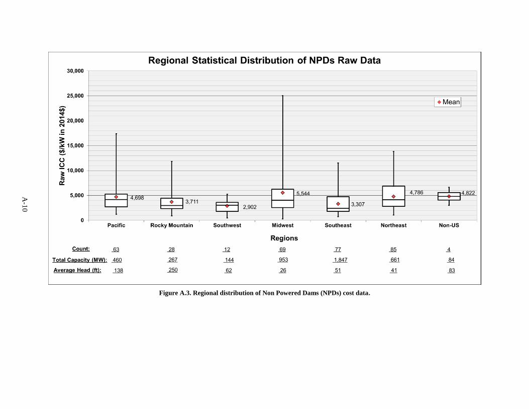
A-1

0

Figure A.3. Regional distribution of Non Powered Dams (NPDs) cost data.

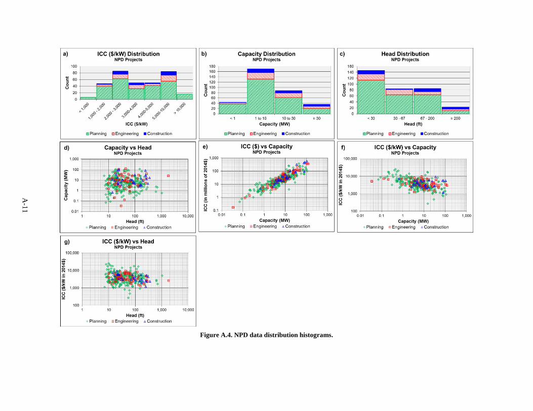
A-1

1

Figure A.4. NPD data distribution histograms.

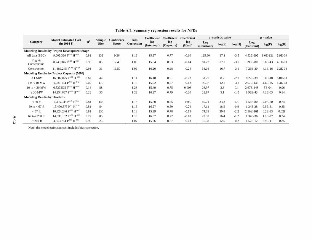
A-1

2

Table A.7. Summary regression results for NPDs

Category Model Estimated Cost

(in 2014 $) R2

Sample

Size

Confidence

Score

Bias

Correction

Coefficient

log

(Intercept)

Coefficient

log

(Capacity)

Coefficient

log

(Head)

t - statistic value p - value

Log

(Constant) log(P) log(H)

Log


Modeling Results by Project Development Stage

All data (PEC) 9,005,320 P0.77 H-0.10 0.81 338 9.26 1.16 15.87 0.77 -0.10 135.90 37.1 -3.5 4.52E-295 8.0E-121 5.9E-04

Eng. &

Construction 8,249,346 P0.93 H-0.14 0.90 85 12.43 1.09 15.84 0.93 -0.14 81.22 27.3 -3.0 3.98E-80 5.8E-43 4.1E-03

Construction 11,489,245 P0.98 H-0.24 0.91 31 13.50 1.06 16.20 0.98 -0.24 54.04 16.7 -3.9 7.29E-30 4.1E-16 6.2E-04

Modeling Results by Project Capacity (MW)

< 1 MW 16,387,025 P0.91 H-0.22 0.62 44 1.14 16.48 0.91 -0.22 51.27 8.2 -2.9 8.22E-39 3.0E-10 6.0E-03

1 to < 10 MW 9,031,154 P0.77 H-0.12 0.49 170 1.10 15.92 0.77 -0.12 96.37 12.3 -3.3 2.67E-148 4.6E-25 1.4E-03

10 to < 30 MW 6,527,525 P0.75 H0.003 0.14 88 1.23 15.49 0.75 0.003 26.97 3.6 0.1 2.67E-148 5E-04 0.96

≥ 30 MW 14,154,867 P0.79 H-0.20 0.28 36 1.22 16.27 0.79 -0.20 13.87 3.1 -1.5 1.98E-43 4.1E-03 0.14

Modeling Results by Head (ft)

< 30 ft 6,395,945 P0.75 H0.05 0.81 146 1.18 15.50 0.75 0.05 40.71 23.2 0.3 1.56E-80 2.0E-50 0.74

30 to < 67 ft 13,490,873 P0.8 H-0.24 0.81 84 1.16 16.27 0.80 -0.24 17.11 18.5 -0.9 1.24E-28 9.5E-31 0.35

< 67 ft 10,324,246 P0.78 H-0.15 0.81 230 1.18 15.99 0.78 -0.15 74.39 30.8 -2.2 2.10E-161 6.2E-83 0.029

67 to< 200 ft 14,530,182 P0.72 H-0.18 0.77 85 1.13 16.37 0.72 -0.18 22.33 16.4 -1.2 1.34E-36 1.1E-27 0.24

≥ 200 ft 4,553,754 P0.87 H-0.03 0.90 23 1.07 15.26 0.87 -0.03 15.38 12.5 -0.2 1.52E-12 6.9E-11 0.85

Note: the model estimated cost includes bias correction.

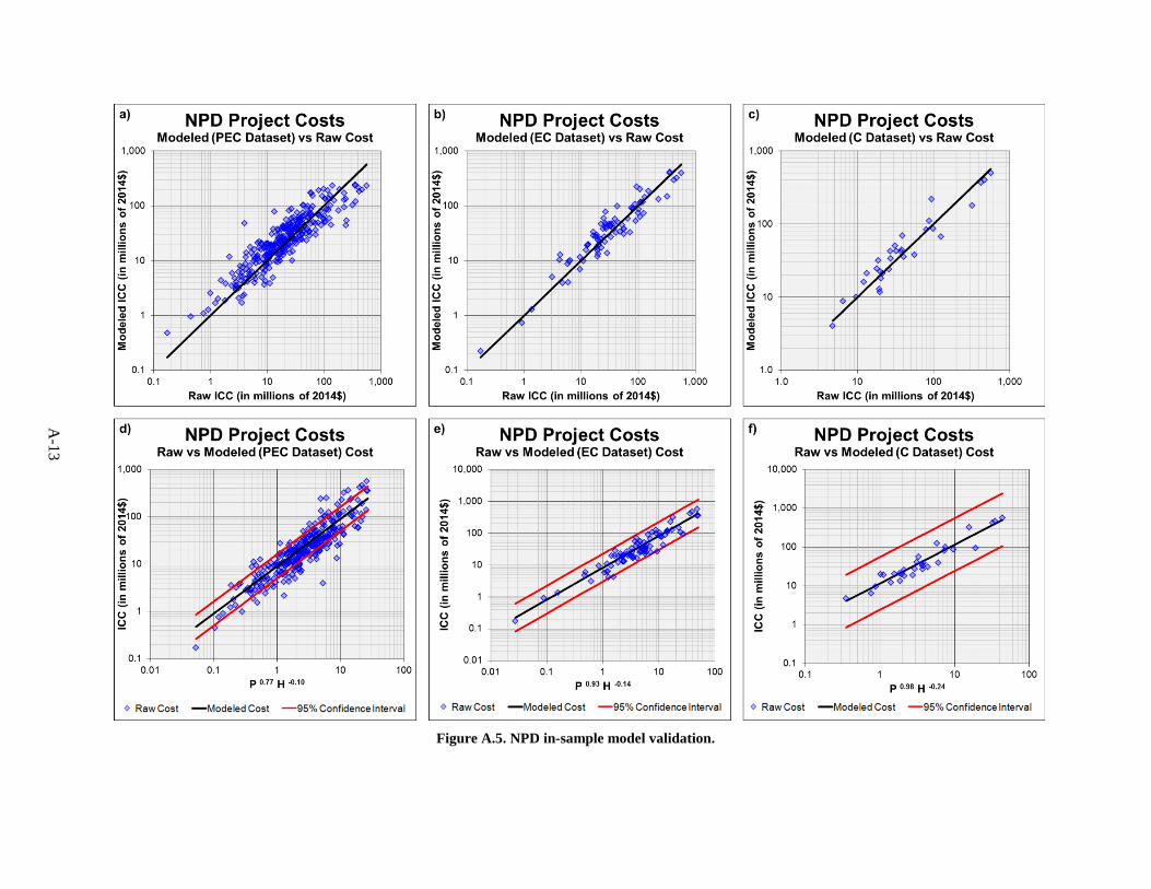
A-1

3

Figure A.5. NPD in-sample model validation.

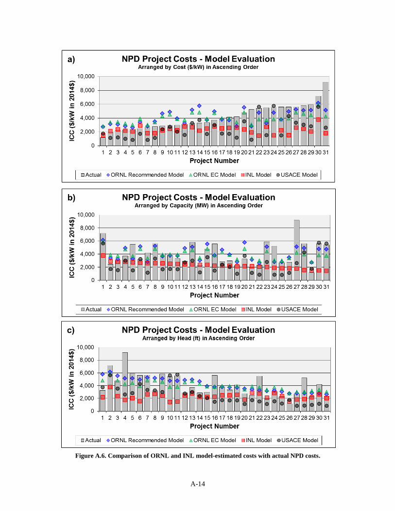
A-14

Figure A.6. Comparison of ORNL and INL model-estimated costs with actual NPD costs.

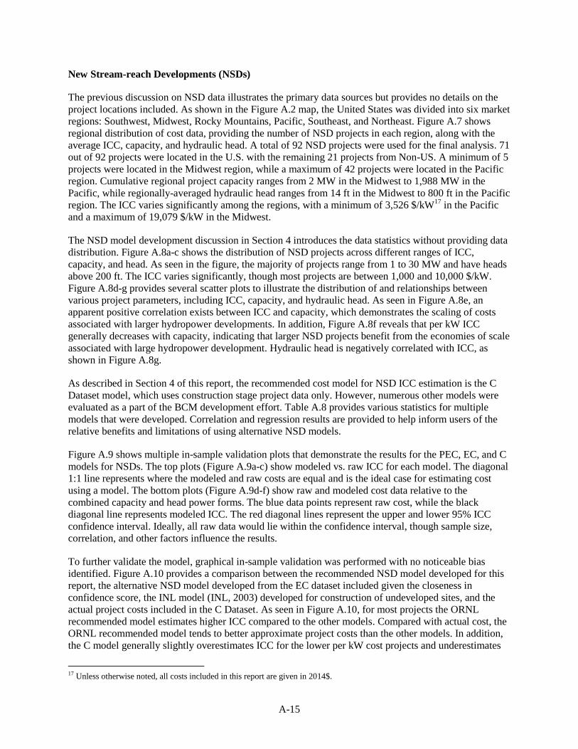
A-15

New Stream-reach Developments (NSDs)

The previous discussion on NSD data illustrates the primary data sources but provides no details on the

project locations included. As shown in the Figure A.2 map, the United States was divided into six market

regions: Southwest, Midwest, Rocky Mountains, Pacific, Southeast, and Northeast. Figure A.7 shows

regional distribution of cost data, providing the number of NSD projects in each region, along with the

average ICC, capacity, and hydraulic head. A total of 92 NSD projects were used for the final analysis. 71

out of 92 projects were located in the U.S. with the remaining 21 projects from Non-US. A minimum of 5

projects were located in the Midwest region, while a maximum of 42 projects were located in the Pacific

region. Cumulative regional project capacity ranges from 2 MW in the Midwest to 1,988 MW in the

Pacific, while regionally-averaged hydraulic head ranges from 14 ft in the Midwest to 800 ft in the Pacific

region. The ICC varies significantly among the regions, with a minimum of 3,526 $/kW17

in the Pacific

and a maximum of 19,079 $/kW in the Midwest.

The NSD model development discussion in Section 4 introduces the data statistics without providing data

distribution. Figure A.8a-c shows the distribution of NSD projects across different ranges of ICC,

capacity, and head. As seen in the figure, the majority of projects range from 1 to 30 MW and have heads

above 200 ft. The ICC varies significantly, though most projects are between 1,000 and 10,000 $/kW.

Figure A.8d-g provides several scatter plots to illustrate the distribution of and relationships between

various project parameters, including ICC, capacity, and hydraulic head. As seen in Figure A.8e, an

apparent positive correlation exists between ICC and capacity, which demonstrates the scaling of costs

associated with larger hydropower developments. In addition, Figure A.8f reveals that per kW ICC

generally decreases with capacity, indicating that larger NSD projects benefit from the economies of scale

associated with large hydropower development. Hydraulic head is negatively correlated with ICC, as

shown in Figure A.8g.

As described in Section 4 of this report, the recommended cost model for NSD ICC estimation is the C

Dataset model, which uses construction stage project data only. However, numerous other models were

evaluated as a part of the BCM development effort. Table A.8 provides various statistics for multiple

models that were developed. Correlation and regression results are provided to help inform users of the

relative benefits and limitations of using alternative NSD models.

Figure A.9 shows multiple in-sample validation plots that demonstrate the results for the PEC, EC, and C

models for NSDs. The top plots (Figure A.9a-c) show modeled vs. raw ICC for each model. The diagonal

1:1 line represents where the modeled and raw costs are equal and is the ideal case for estimating cost

using a model. The bottom plots (Figure A.9d-f) show raw and modeled cost data relative to the

combined capacity and head power forms. The blue data points represent raw cost, while the black

diagonal line represents modeled ICC. The red diagonal lines represent the upper and lower 95% ICC

confidence interval. Ideally, all raw data would lie within the confidence interval, though sample size,

correlation, and other factors influence the results.


identified. Figure A.10 provides a comparison between the recommended NSD model developed for this

report, the alternative NSD model developed from the EC dataset included given the closeness in

confidence score, the INL model (INL, 2003) developed for construction of undeveloped sites, and the

actual project costs included in the C Dataset. As seen in Figure A.10, for most projects the ORNL

recommended model estimates higher ICC compared to the other models. Compared with actual cost, the

ORNL recommended model tends to better approximate project costs than the other models. In addition,

the C model generally slightly overestimates ICC for the lower per kW cost projects and underestimates


A-16

ICC for the higher per kW cost projects (Figure A.10a). As seen in Figure A.10b and Figure A.10c, the

recommended model’s relative error is largely independent of variation in capacity and head. Compared

with the EC model, the recommended model provides very similar ICC estimates, though a more

noticeable difference is seen for the lower and higher head projects (Figure A.10c). The INL model shows

significant bias in estimating ICC for both low and high head projects, as the model provides only a

univariate estimate based on capacity (Figure A.10c). The average actual per kW project ICC for the 18

constructed projects is $4,156, while the recommended ORNL and INL models produce average per kW

costs of $4,140 and $1,859, respectively. As the recommended ORNL model was developed based on

regression analysis using the same set of 18 constructed projects, the model necessarily produces the best

approximation for the actual cost, and further data collection will allow for the model to be benchmarked

against out of sample data points, and more robustly identify cost drivers at the component level.

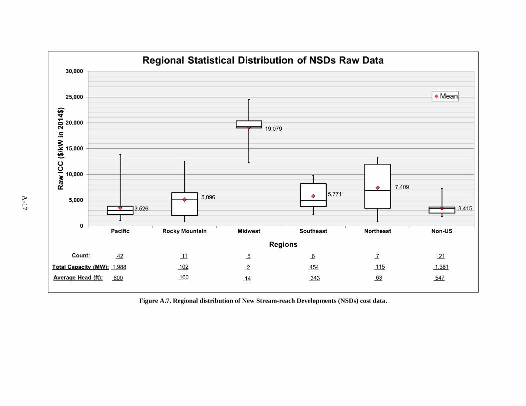
A-1

7

Figure A.7. Regional distribution of New Stream-reach Developments (NSDs) cost data.

A-1

8

Figure A.8. NSD data distribution histograms.

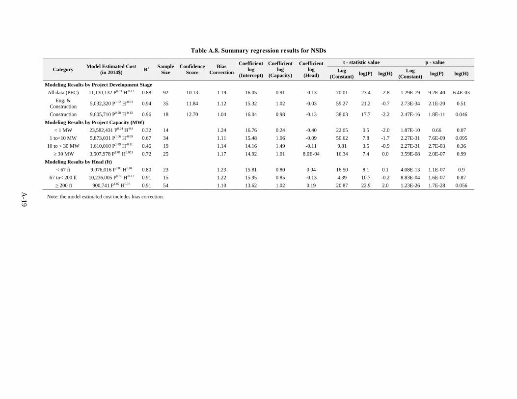
A-1

9

Table A.8. Summary regression results for NSDs


(in 2014$) R2

Sample

Size

Confidence

Score

Bias

Correction

Coefficient

log

(Intercept)

Coefficient

log

(Capacity)

Coefficient

log

(Head)


Log


Log



All data (PEC) 11,130,132 P0.91 H-0.13 0.88 92 10.13 1.19 16.05 0.91 -0.13 70.01 23.4 -2.8 1.29E-79 9.2E-40 6.4E-03

Eng. &

Construction 5,032,320 P1.02 H-0.03 0.94 35 11.84 1.12 15.32 1.02 -0.03 59.27 21.2 -0.7 2.73E-34 2.1E-20 0.51



< 1 MW 23,582,431 P0.24 H-0.4 0.32 14 1.24 16.76 0.24 -0.40 22.05 0.5 -2.0 1.87E-10 0.66 0.07

1 to<10 MW 5,873,031 P1.06 H-0.09 0.67 34 1.11 15.48 1.06 -0.09 50.62 7.8 -1.7 2.27E-31 7.6E-09 0.095

10 to < 30 MW 1,610,010 P1.49 H-0.11 0.46 19 1.14 14.16 1.49 -0.11 9.81 3.5 -0.9 2.27E-31 2.7E-03 0.36

≥ 30 MW 3,507,978 P1.01 H0.001 0.72 25 1.17 14.92 1.01 8.0E-04 16.34 7.4 0.0 3.59E-08 2.0E-07 0.99


< 67 ft 9,076,016 P0.80 H0.04 0.80 23 1.23 15.81 0.80 0.04 16.50 8.1 0.1 4.08E-13 1.1E-07 0.9

67 to< 200 ft 10,236,005 P0.85 H-0.13 0.91 15 1.22 15.95 0.85 -0.13 4.39 10.7 -0.2 8.83E-04 1.6E-07 0.87

≥ 200 ft 900,741 P1.02 H0.19 0.91 54 1.10 13.62 1.02 0.19 20.87 22.9 2.0 1.23E-26 1.7E-28 0.056


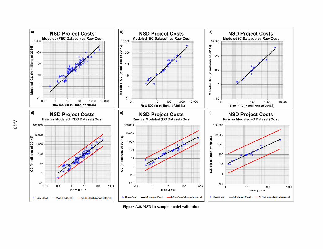
A-2

0

Figure A.9. NSD in-sample model validation.

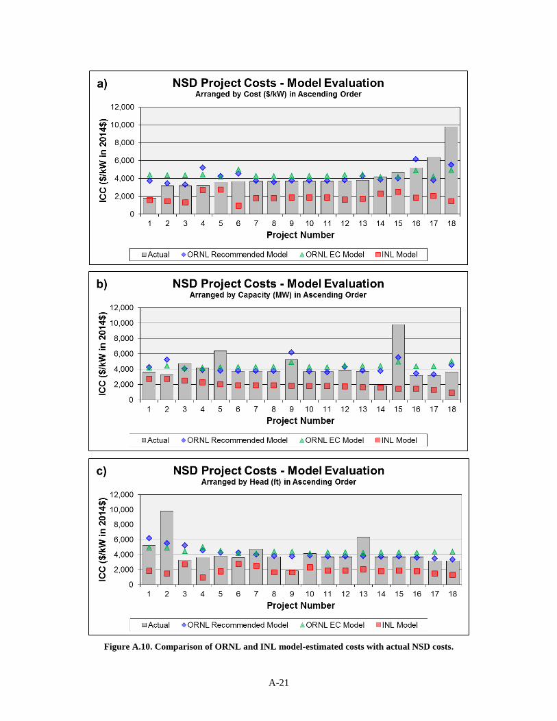
A-21

Figure A.10. Comparison of ORNL and INL model-estimated costs with actual NSD costs.

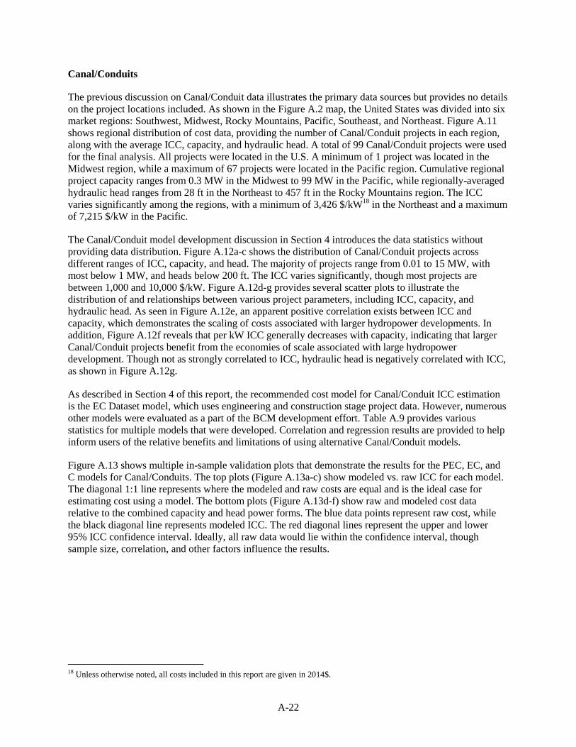
A-22

Canal/Conduits

The previous discussion on Canal/Conduit data illustrates the primary data sources but provides no details

on the project locations included. As shown in the Figure A.2 map, the United States was divided into six

market regions: Southwest, Midwest, Rocky Mountains, Pacific, Southeast, and Northeast. Figure A.11

shows regional distribution of cost data, providing the number of Canal/Conduit projects in each region,

along with the average ICC, capacity, and hydraulic head. A total of 99 Canal/Conduit projects were used

for the final analysis. All projects were located in the U.S. A minimum of 1 project was located in the

Midwest region, while a maximum of 67 projects were located in the Pacific region. Cumulative regional

project capacity ranges from 0.3 MW in the Midwest to 99 MW in the Pacific, while regionally-averaged

hydraulic head ranges from 28 ft in the Northeast to 457 ft in the Rocky Mountains region. The ICC

varies significantly among the regions, with a minimum of 3,426 $/kW18

in the Northeast and a maximum

of 7,215 $/kW in the Pacific.

The Canal/Conduit model development discussion in Section 4 introduces the data statistics without

providing data distribution. Figure A.12a-c shows the distribution of Canal/Conduit projects across

different ranges of ICC, capacity, and head. The majority of projects range from 0.01 to 15 MW, with

most below 1 MW, and heads below 200 ft. The ICC varies significantly, though most projects are

between 1,000 and 10,000 $/kW. Figure A.12d-g provides several scatter plots to illustrate the

distribution of and relationships between various project parameters, including ICC, capacity, and

hydraulic head. As seen in Figure A.12e, an apparent positive correlation exists between ICC and

capacity, which demonstrates the scaling of costs associated with larger hydropower developments. In

addition, Figure A.12f reveals that per kW ICC generally decreases with capacity, indicating that larger

Canal/Conduit projects benefit from the economies of scale associated with large hydropower

development. Though not as strongly correlated to ICC, hydraulic head is negatively correlated with ICC,

as shown in Figure A.12g.

As described in Section 4 of this report, the recommended cost model for Canal/Conduit ICC estimation

is the EC Dataset model, which uses engineering and construction stage project data. However, numerous

other models were evaluated as a part of the BCM development effort. Table A.9 provides various

statistics for multiple models that were developed. Correlation and regression results are provided to help

inform users of the relative benefits and limitations of using alternative Canal/Conduit models.

Figure A.13 shows multiple in-sample validation plots that demonstrate the results for the PEC, EC, and

C models for Canal/Conduits. The top plots (Figure A.13a-c) show modeled vs. raw ICC for each model.

The diagonal 1:1 line represents where the modeled and raw costs are equal and is the ideal case for

estimating cost using a model. The bottom plots (Figure A.13d-f) show raw and modeled cost data

relative to the combined capacity and head power forms. The blue data points represent raw cost, while

the black diagonal line represents modeled ICC. The red diagonal lines represent the upper and lower

95% ICC confidence interval. Ideally, all raw data would lie within the confidence interval, though

sample size, correlation, and other factors influence the results.


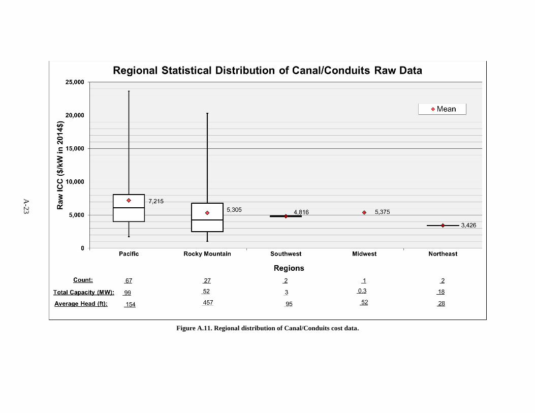
A-2

3

Figure A.11. Regional distribution of Canal/Conduits cost data.

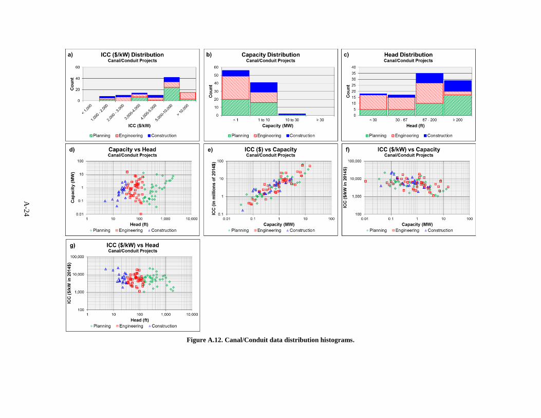
A-2

4

Figure A.12. Canal/Conduit data distribution histograms.

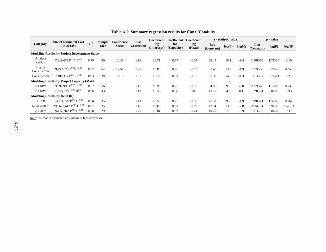
A-2

5

Table A.9. Summary regression results for Canal/Conduits


(in 2014$) R2

Sample

Size

Confidence

Score

Bias

Correction

Coefficient

log

(Intercept)

Coefficient

log

(Capacity)

Coefficient

log

(Head)


Log


Log



All data

(PEC) 7,819,672 P0.79 H-0.07 0.79 99 10.40 1.18 15.71 0.79 -0.07 68.44 19.1 -1.4 2.80E-83 1.7E-34 0.16

Eng. &




< 1 MW 9,292,909 P0.77 H-0.13 0.67 56

1.15 15.90 0.77 -0.13 54.86 9.9 -2.0 2.27E-48 1.1E-13 0.048

≥ 1 MW 6,975,229 P0.58 H0.01 0.36 43

1.19 15.58 0.58 0.01 41.77 4.6 0.1 1.29E-34 3.8E-05 0.93


< 67 ft 16,171,129 P0.75 H-0.33 0.74 35

1.11 16.50 0.75 -0.33 27.57 9.2 -1.9 7.19E-24 1.5E-10 0.062

67 to<200 ft 398,622,447 P0.81 H-0.92 0.87 35

1.15 19.66 0.81 -0.92 12.94 13.6 -2.8 2.95E-14 6.9E-15 8.5E-03

≥ 200 ft 24,658,942 P0.82 H-0.24 0.78 29 1.20 16.84 0.82 -0.24 10.27 7.3 -0.9 1.21E-10 9.0E-08 0.37


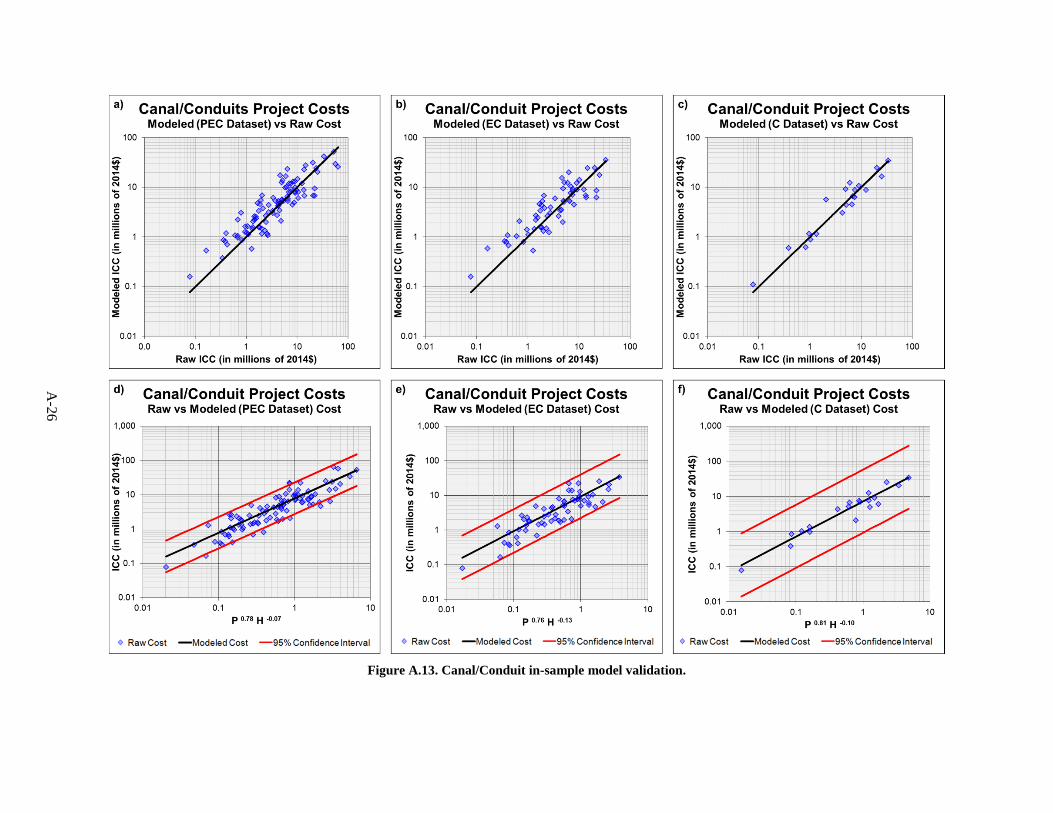
A-2

6

Figure A.13. Canal/Conduit in-sample model validation.

A-27

Unit Addition and Generator Rewind

The previous discussion on Unit Addition and Generator Rewind data illustrates the primary data sources

but provides no details on the project locations included. As shown in the Figure A.2 map, the United

States was divided into six market regions: Southwest, Midwest, Rocky Mountains, Pacific, Southeast,

and Northeast. Figure A.14 and Figure A.15 show regional distribution of cost data, providing the number

of projects in each region, along with the average ICC and total capacity for Unit Addition and Generator

Rewind respectively. No Unit Addition project data were available for the Southeast region. Also, no

Generator Rewind data were available for the Midwest region. A total of 17 Unit Addition and 27

Generator Rewind projects were used for the final analysis.

Table A.10 provides a summary of various statistics for each model that was developed for Unit Addition

and Generator Rewind in Section 4. As the raw data were limited to a relatively small sample size, only

the PEC Model was developed. Figure A.16a-b shows in-sample validation plots that illustrate the model

results. The modeled vs. raw ICC with the diagonal 1:1 line represents the points at which the modeled

and raw costs are equal. Figure A.16c-d shows raw and modeled cost data relative to the capacity power

form. The blue points represent raw cost, while the black diagonal line represents modeled ICC. The red

diagonal lines represent the upper and lower 95% confidence interval ICC. Ideally, all raw data would lie

within the confidence interval, though sample size, correlation, and other factors influence the results.

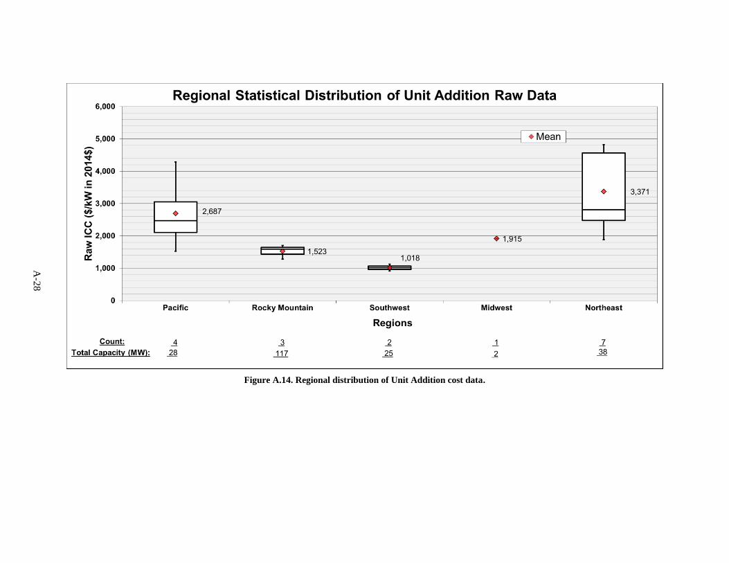
A-2

8

Figure A.14. Regional distribution of Unit Addition cost data.

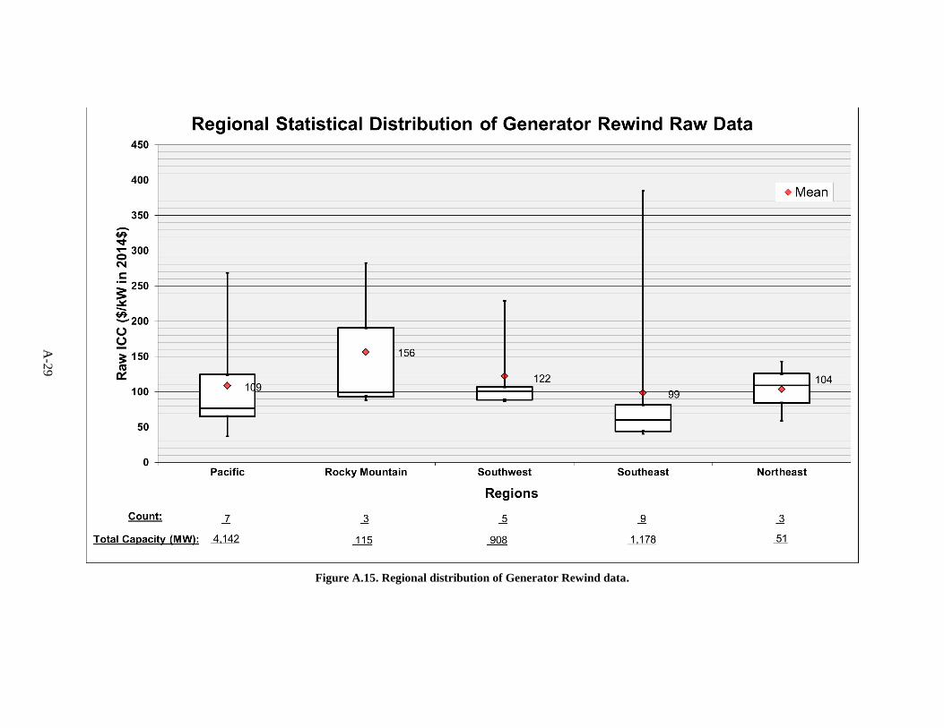
A-2

9

Figure A.15. Regional distribution of Generator Rewind data.

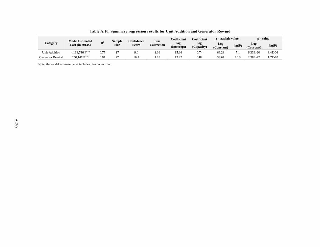
A-3

0

Table A.10. Summary regression results for Unit Addition and Generator Rewind

Category Model Estimated

Cost (in 2014$) R2

Sample

Size

Confidence

Score

Bias

Correction

Coefficient

log

(Intercept)

Coefficient

log

(Capacity)


Log

(Constant) log(P)

Log

(Constant) log(P)

Unit Addition 4,163,746 P0.74 0.77 17 9.0 1.09 15.16 0.74 66.23 7.1 6.33E-20 3.4E-06

Generator Rewind 250,147 P0.82 0.81 27 10.7 1.18 12.27 0.82 33.67 10.3 2.38E-22 1.7E-10


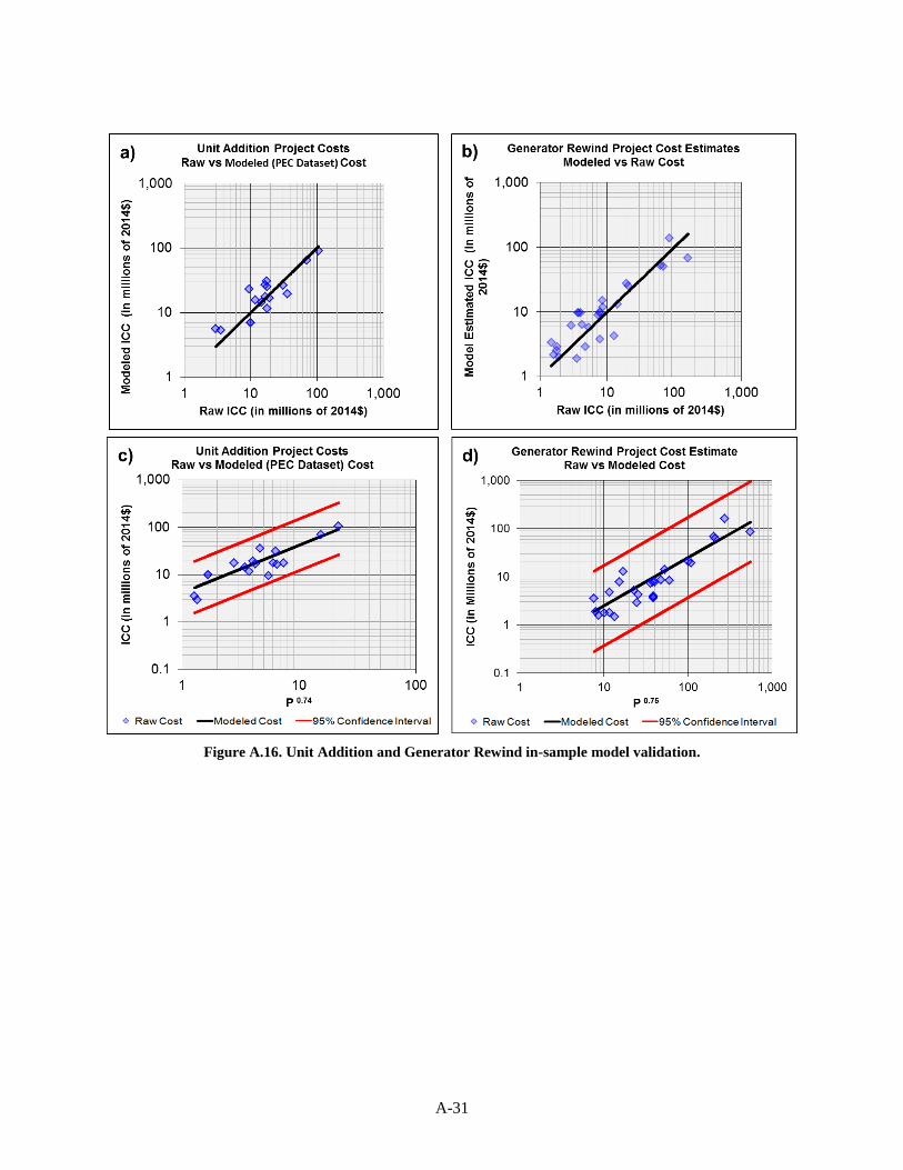
A-31

Figure A.16. Unit Addition and Generator Rewind in-sample model validation.

APPENDIX B. CONFIDENCE SCORE CRITERIA

B-3

APPENDIX B. CONFIDENCE SCORE CRITERIA

Model Confidence Scoring

In the development of the BCMs, a variety of different data subsets were evaluated both to understand the

sources of cost variation and to ultimately select the models that best represent the cost of developing the

remaining U.S. hydropower resources. To consistently evaluate the alternative model options within each

resource class, a quantitative evaluation system was developed to rank models based on the following

series of metrics related to (1) attributes of the data used in the development of the model, and (2) the

overall quality of the model itself:

Data

o Data Quality (project development stage)

o Data Scope and Consistency

o Data Vintage (age of cost estimate)

Model Quality

o Sample Size

o Data QA/QC

o Goodness of Fit

o Validation

o Application Range

Table B.1 shows how the metrics used for evaluating model confidence are quantified. The confidence

level associated with each data source are quantified using Items 1 through 3, while the overall model

results, reliability, and application are scored using Items 4 through 8. Individual model scores for Items 1

and 3 are weighted according to the number of projects included from each development stage and

vintage category, respectively. A model confidence score in this report is sum of score of each item 1 to 8.

Overall, the range of potential confidence scores range from 0 to 17. In BCM report, a recommended

model is identified based on confidence score results.

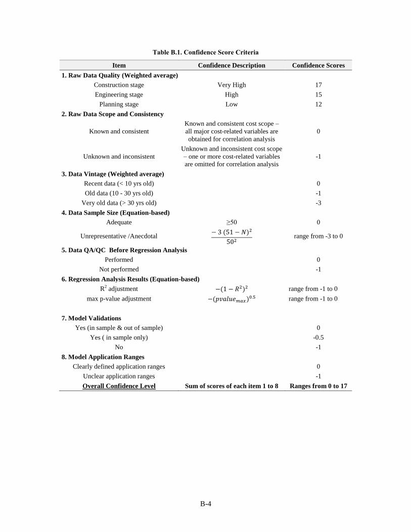
B-4

Table B.1. Confidence Score Criteria

Item Confidence Description Confidence Scores

1. Raw Data Quality (Weighted average)

Construction stage Very High 17

Engineering stage High 15

Planning stage Low 12

2. Raw Data Scope and Consistency

Known and consistent

Known and consistent cost scope –

all major cost-related variables are

obtained for correlation analysis

0

Unknown and inconsistent

Unknown and inconsistent cost scope

– one or more cost-related variables

are omitted for correlation analysis

-1

3. Data Vintage (Weighted average)

Recent data (< 10 yrs old)

0

Old data (10 - 30 yrs old)

-1

Very old data (> 30 yrs old)

-3

4. Data Sample Size (Equation-based)

Adequate ≥50 0

Unrepresentative /Anecdotal − 3 (51 − 𝑁)2

502 range from -3 to 0

5. Data QA/QC Before Regression Analysis

Performed

0

Not performed

-1

6. Regression Analysis Results (Equation-based)

R2 adjustment −(1 − 𝑅2)2 range from -1 to 0

max p-value adjustment −(𝑝𝑣𝑎𝑙𝑢𝑒𝑚𝑎𝑥)0.5 range from -1 to 0

7. Model Validations

Yes (in sample & out of sample)

0

Yes ( in sample only)

-0.5

No

-1

8. Model Application Ranges

Clearly defined application ranges

0

Unclear application ranges

-1

Overall Confidence Level Sum of scores of each item 1 to 8 Ranges from 0 to 17

APPENDIX C. O&M DATA SOURCES, ALTERNATIVE MODELS,

AND VALIDATION

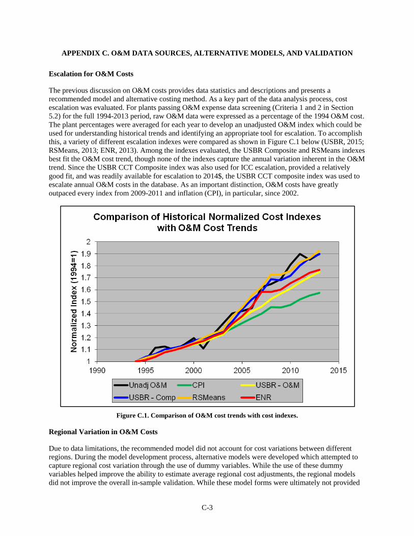
C-3

APPENDIX C. O&M DATA SOURCES, ALTERNATIVE MODELS, AND VALIDATION

Escalation for O&M Costs

The previous discussion on O&M costs provides data statistics and descriptions and presents a

recommended model and alternative costing method. As a key part of the data analysis process, cost

escalation was evaluated. For plants passing O&M expense data screening (Criteria 1 and 2 in Section

5.2) for the full 1994-2013 period, raw O&M data were expressed as a percentage of the 1994 O&M cost.

The plant percentages were averaged for each year to develop an unadjusted O&M index which could be

used for understanding historical trends and identifying an appropriate tool for escalation. To accomplish

this, a variety of different escalation indexes were compared as shown in Figure C.1 below (USBR, 2015;

RSMeans, 2013; ENR, 2013). Among the indexes evaluated, the USBR Composite and RSMeans indexes

best fit the O&M cost trend, though none of the indexes capture the annual variation inherent in the O&M

trend. Since the USBR CCT Composite index was also used for ICC escalation, provided a relatively

good fit, and was readily available for escalation to 2014$, the USBR CCT composite index was used to

escalate annual O&M costs in the database. As an important distinction, O&M costs have greatly

outpaced every index from 2009-2011 and inflation (CPI), in particular, since 2002.

Figure C.1. Comparison of O&M cost trends with cost indexes.

Regional Variation in O&M Costs

Due to data limitations, the recommended model did not account for cost variations between different

regions. During the model development process, alternative models were developed which attempted to

capture regional cost variation through the use of dummy variables. While the use of these dummy

variables helped improve the ability to estimate average regional cost adjustments, the regional models

did not improve the overall in-sample validation. While these model forms were ultimately not provided

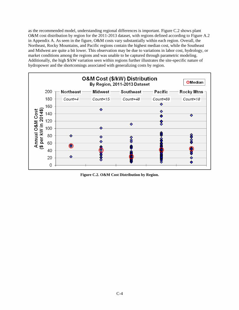
C-4

as the recommended model, understanding regional differences is important. Figure C.2 shows plant

O&M cost distribution by region for the 2011-2013 dataset, with regions defined according to Figure A.2

in Appendix A. As seen in the figure, O&M costs vary substantially within each region. Overall, the

Northeast, Rocky Mountains, and Pacific regions contain the highest median cost, while the Southeast

and Midwest are quite a bit lower. This observation may be due to variations in labor cost, hydrology, or

market conditions among the regions and was unable to be captured through parametric modeling.

Additionally, the high $/kW variation seen within regions further illustrates the site-specific nature of

hydropower and the shortcomings associated with generalizing costs by region.

Figure C.2. O&M Cost Distribution by Region.

C-5

O&M Regression Results for Alternative Models

As described in Section 5.5 of this report, the recommended cost model for O&M results from the use of

the 2011-2013 dataset and capacity as an independent variable; however, other models were evaluated as

part of the BCM development efforts.

Table C.1 provides various statistics for multiple models that were developed using combinations of

capacity, head, and generation as independent variables for different datasets. These models were

developed without regional dummy variables and demonstrate that capacity, head, and generation all

correlate well with O&M costs; however, the majority of the variation in cost is explained through

capacity variations alone. Correlation and regression results are provided to help inform users of the

relative benefits and limitations of using alternative O&M models. Table C.2 includes model results

which account for regional cost variation through the use of dummy variables. Regional O&M cost

models are reported for capacity-only models, as the addition of dummy variables resulted in lower p-

values for the other independent variables.

Figure C.3 provides an illustration of in-sample model validation performed for the recommended model.

Figure C.3a demonstrates a good overall fit; however, variation exists. As shown in Figure C.3b, several

data points lie outside of the 95 percent confidence interval, which is expected, since the screening

process involved in developing the recommended model only removed outliers beyond 2.5 standard

residuals from the mean (which roughly translates to a 98.8 percent confidence interval using Z-score

methodology).

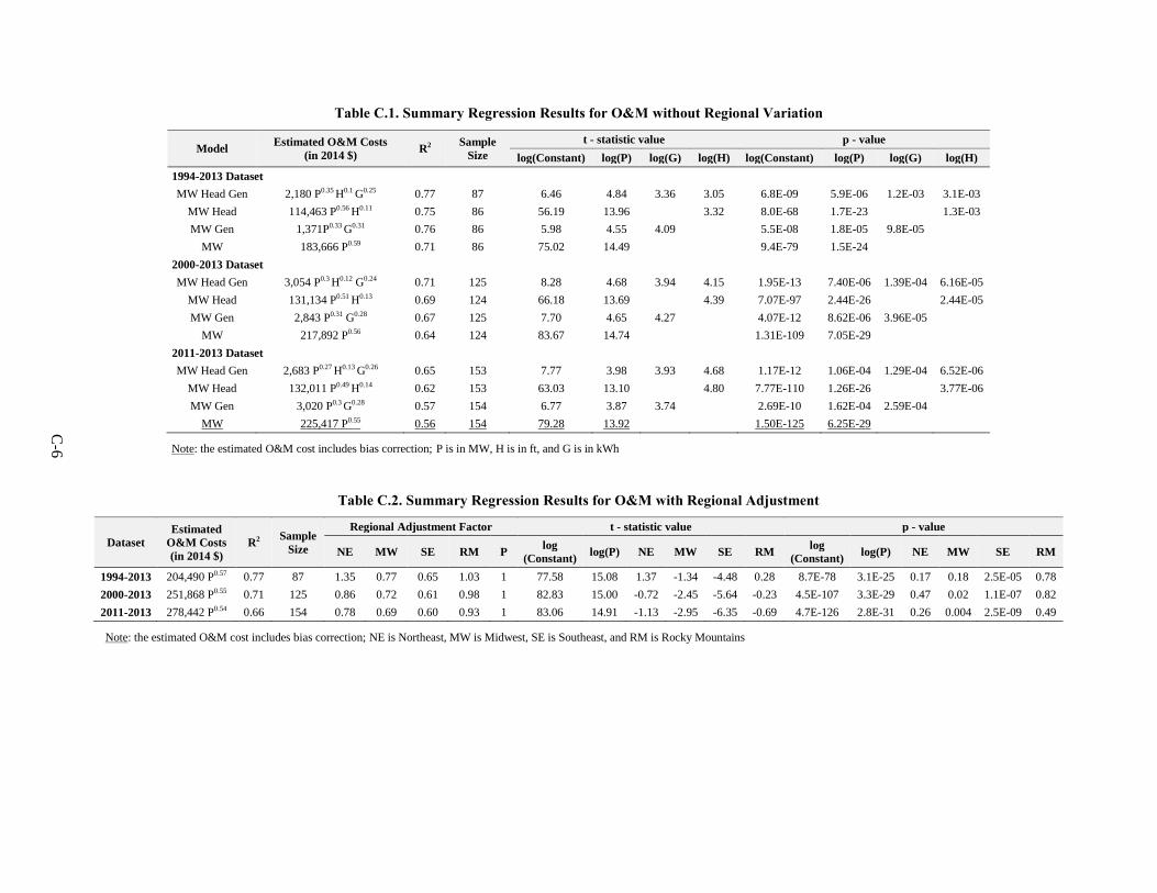
C-6

Table C.1. Summary Regression Results for O&M without Regional Variation

Model Estimated O&M Costs

(in 2014 $) R2

Sample

Size


log(Constant) log(P) log(G) log(H) log(Constant) log(P) log(G) log(H)

1994-2013 Dataset

MW Head Gen 2,180 P0.35 H0.1 G0.25 0.77 87 6.46 4.84 3.36 3.05 6.8E-09 5.9E-06 1.2E-03 3.1E-03

MW Head 114,463 P0.56 H0.11 0.75 86 56.19 13.96

3.32 8.0E-68 1.7E-23

1.3E-03

MW Gen 1,371P0.33 G0.31 0.76 86 5.98 4.55 4.09

5.5E-08 1.8E-05 9.8E-05

MW 183,666 P0.59 0.71 86 75.02 14.49

9.4E-79 1.5E-24

2000-2013 Dataset


MW Head 131,134 P0.51 H0.13 0.69 124 66.18 13.69

4.39 7.07E-97 2.44E-26

2.44E-05

MW Gen 2,843 P0.31 G0.28 0.67 125 7.70 4.65 4.27

4.07E-12 8.62E-06 3.96E-05

MW 217,892 P0.56 0.64 124 83.67 14.74

1.31E-109 7.05E-29

2011-2013 Dataset


MW Head 132,011 P0.49 H0.14 0.62 153 63.03 13.10

4.80 7.77E-110 1.26E-26

3.77E-06

MW Gen 3,020 P0.3 G0.28 0.57 154 6.77 3.87 3.74

2.69E-10 1.62E-04 2.59E-04

MW 225,417 P0.55 0.56 154 79.28 13.92

1.50E-125 6.25E-29

Note: the estimated O&M cost includes bias correction; P is in MW, H is in ft, and G is in kWh

Table C.2. Summary Regression Results for O&M with Regional Adjustment

Dataset

Estimated

O&M Costs

(in 2014 $)

R2 Sample

Size

Regional Adjustment Factor t - statistic value p - value

NE MW SE RM P log

(Constant) log(P) NE MW SE RM

log

(Constant) log(P) NE MW SE RM

1994-2013 204,490 P0.57 0.77 87 1.35 0.77 0.65 1.03 1 77.58 15.08 1.37 -1.34 -4.48 0.28 8.7E-78 3.1E-25 0.17 0.18 2.5E-05 0.78

2000-2013 251,868 P0.55 0.71 125 0.86 0.72 0.61 0.98 1 82.83 15.00 -0.72 -2.45 -5.64 -0.23 4.5E-107 3.3E-29 0.47 0.02 1.1E-07 0.82

2011-2013 278,442 P0.54 0.66 154 0.78 0.69 0.60 0.93 1 83.06 14.91 -1.13 -2.95 -6.35 -0.69 4.7E-126 2.8E-31 0.26 0.004 2.5E-09 0.49

Note: the estimated O&M cost includes bias correction; NE is Northeast, MW is Midwest, SE is Southeast, and RM is Rocky Mountains

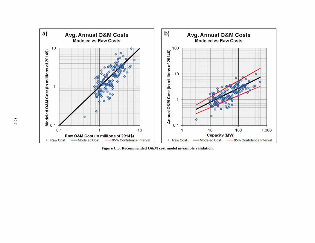
C-7

Figure C.3. Recommended O&M cost model in-sample validation.

Documents

Hydropower Baseline Cost Modeling, Version 2