Embed Size (px)
Citation preview
Hydrologic impacts of Landuse change in the
Upper Gilgel Abay River Basin, Ethiopia;
TOPMODEL Application.
Webster Gumindoga
February, 2010
Hydrologic impacts of Landuse change in the Upper
Gilgel Abay River Basin, Ethiopia; TOPMODEL
Application.
by
Webster Gumindoga
Thesis submitted to the International Institute for Geo-information Science and Earth Observation in
partial fulfilment of the requirements for the degree of Master of Science in Geo-information Science
and Earth Observation, Specialisation: Integrated Watershed Management and Modelling
(Surface Hydrology)
Thesis Assessment Board
Dr. Ir. M.W. Lubczynski (Chairman) WREM dept., ITC, Enschede
Dr. Ir. P. Reggiani (External Examiner) Deltaris, Delft
Dr. Ir. T.H.M Rientjes (First Supervisor) WREM dept. ITC, Enschede
Dr. A.S.M Gieske (Second Supervisor) WREM dept. ITC, Enschede
Mr. Alemseged Tamiru Haile (Advisor) WREM dept. ITC, Enschede

INTERNATIONAL INSTITUTE FOR GEO-INFORMATION SCIENCE AND EARTH OBSERVATION
ENSCHEDE, THE NETHERLANDS

Disclaimer
This document describes work undertaken as part of a programme of study at the International
Institute for Geo-information Science and Earth Observation. All views and opinions expressed
therein remain the sole responsibility of the author, and do not necessarily represent those of the
institute.

Dedications
Dedicated to my parents Mr and Mrs T.E Gumindoga.
i
Abstract
Landuse and landcover change affect the different hydrological components like interception, infiltration
and evaporation thereby influencing runoff generation (both process and volume) and streamflow
regimes. Comparatively, little is known about factors that affect runoff behaviour and their relation to
landuse in a data poor catchment like the Upper Gilgel Abay basin. Remote sensing was therefore used
in this study to observe catchment characteristics and to estimate the model parameters that reflect on
the land surface characteristics. Firstly, the TOPMODEL approach was applied to simulate streamflow
for this basin. An ASTER 30m DEM was used to compute the topographic Index, critical for the
simulation of streamflow in the basin. Results of calibration gave a Nash-Sutcliffe model efficiency
(NS) of 0.81 and a Relative Volume Error (RVE) of 6.1%. Sensitivity analysis of the model showed that
the parameters most critical for accurately simulating runoff were: the exponential transmissivity
function (m), the soil transmissivity at saturation (To) and the root zone available water capacity
(SRmax). The model was validated using a 2003 meteorological dataset and a satisfactory model
performance was obtained (NS=0.75, RVE= -4.0 %). GIS and remote sensing were further used for the
quantification of vegetation indices such as SAVI and LAI. Rainfall interception as a function of LAI
from different vegetation types was determined. The implementation of landuse in TOPMODEL was
done by treatment of each vegetation/landuse type as a ‘subcatchment’ through a GIS overlay of landuse
types thus creating a topographic index distribution for each landuse type. These were run separately
with specific landuse parameters. The areally weighted results were summed to get a total output
imitating having multiple subcatchments with different topographic index distributions. Results showed
that the maximum peakflow from agricultural land increased by 51% from 1973-1986 and by 44%
between 1986 and 2001. Annual runoff volume increased by 12% between 1986 and 2001 which
corresponds to increases in agricultural land from 1973 to 2001. From 1973-1986 and from 1986-2001,
forest and shrubland decreased in maximum peakflow by same amount (29%). The annual runoff
volume also decreased by 36% from 1973-1986 and by 34% from 1986-2001. This could be attributed
to decreases in forests between the years 1973, 1986 and 2001. Finally for each year, a comparison was
made between the sum of all landuse simulated discharge and the observed discharge at the outlet. The
following satisfactory model efficiencies were obtained: 1973 (NS=0.81, RVE=5.82 %); 1986
(NS=0.72, RVE=29.72 %) and 2001 (NS=0.73, RVE= 18.50 %). These results prove that in data poor
basins, a promising way to analyse hydrological impacts of land-use change is by combining remote
sensing for land surface parameterization and a semi distributed rainfall-runoff model. The findings also
provide useful support for land use planning and management.
Key words: Upper Gilgel Abay, Land use, Remote sensing, TOPMODEL, Nash–Sutcliffe, Streamflow.

ii

iii
Acknowledgements
I testify of God’s grace that was sufficient for me throughout my studies at ITC.
I would also want to give special thanks to the Netherlands Fellowship Programme (NFP) for
sponsoring my studies in the Netherlands.
Furthermore I would like to thank my first supervisor Dr. Ing. T. H. M. Rientjes for his guidance and
advice in every stage of the project. I greatly acknowledge him for his highly stimulating discussions and
comments and for imparting me his ‘modelling in hydrology’ skills.
I would also want to extent my great appreciation to my second supervisor Dr. A.S.M Gieske for his
support, comments and assistance in programming and handling the IDL code.
The assistance of my advisor Mr. Alemseged Tamiru Haile in this project is also greatly appreciated.
My fieldwork trip and stay in Ethiopia was made easier and possible by his presence. I thank him so
much for sparing his time and keeping me company in Bahir dar.
The special advice of Prof. Keith Beven, the Professor of Hydrology and Fluid Dynamics at the
Lancaster Environment Centre will not go unmentioned. His quick replies and the concept of ‘treating
each vegetation type as a “subcatchment” and creating a topographic index distribution for each
vegetation type’ gave me a good kick start into the issue of landuse simulations using TOPMODEL.
Finally I give special thanks to all my lecturers, who helped me with great ideas throughout the
beginning of the course to the completion of the thesis and of course not forgetting the beautiful WREM
2008-2010 buddies. I am also greatly indebted to my parents, brothers and sisters in Zimbabwe for their
prayers and support. To the Mupamhangas, thanks so much for the motivation and other forms of
support. My friends from ITC Fellowship and the Zimbabwean community at ITC, I thank you so much
for the fellowship we shared.

iv
Table of contents
Abstract .................................................................................................................................. i
Acknowledgements ............................................................................................................... iii
Table of contents................................................................................................................... iv
List of figures ........................................................................................................................ vi
List of tables........................................................................................................................ viii
1. INTRODUCTION ............................................................................................................. 1
1.1. Background ................................................................................................................. 1
1.2. Statement of the problem............................................................................................. 2
1.3. Previous TOPMODEL studies ..................................................................................... 3
1.4. Objectives of the study................................................................................................. 3
1.5. Thesis outline .............................................................................................................. 4
2. STUDY AREA AND LITERATURE REVIEW ................................................................ 6
2.1. Background to the study area ...................................................................................... 6
2.1.1. Geographic location.............................................................................................. 6
2.1.2. Topography .......................................................................................................... 6
2.1.3. Climate ................................................................................................................. 7
2.1.4. Soil....................................................................................................................... 7
2.1.5. Land use and Land cover ...................................................................................... 7
2.2. Literature review: Topmodel approach ........................................................................ 8
2.2.1. Dominant flow processes at the hillslope ............................................................... 8
2.2.2. The Topographic index ......................................................................................... 9
2.2.3. Progression in simulations using TOPMODEL concept ....................................... 10
2.2.4. Assumptions of TOPMODEL ............................................................................. 11
2.2.5. Description of the model and governing equations............................................... 11
2.2.6. What happens in the saturated zone?................................................................... 11
2.2.7. What happens in the unsaturated zone and root zone reservoir?........................... 15
2.2.8. Overland flow and channel network routing ........................................................ 17
2.2.9. Choice of transmissivity profile. .......................................................................... 17
2.2.10. TOPMODEL parameters .................................................................................. 19
2.3. Literature review: Landuse change............................................................................. 21
2.3.1. Remote sensing application on landuse and landcover analysis............................. 21
2.3.2. Vegetation and soil as controlling factors in hillslope hydrology. ......................... 21
2.3.3. Parameterization of landuse change in different hydrological models ................... 22
3. METHODOLOGY........................................................................................................... 25
3.1. Sequence of the research process and methodology. .................................................. 25
3.1.1. Data availability and fieldwork activities.............................................................. 26
3.1.2. Computation of missing values by the simple linear regression method. ............... 26
3.1.3. Validation of the method of filling in missing data ............................................... 27
3.1.4. Evaluation of the rainfall distribution using GIS................................................... 28
3.1.5. Evaporation calculation....................................................................................... 28
3.1.6. Choice of transmissivity profile. .......................................................................... 29
3.1.8. Code modification and version of TOPMODEL applied ...................................... 30
3.1.9. Sensitivity analysis, calibration and validation for TOPMODEL........................... 30

v
3.2. Parameterization of land-use in TOPMODEL. ........................................................... 32
3.2.1. Soil Adjusted Vegetation Index (SAVI) .............................................................. 32
3.2.2. Leaf Area Index (LAI) ........................................................................................ 33
3.2.3. Interception module. ........................................................................................... 33
3.2.4. Evapotranspiration calculated using the crop coefficient approach....................... 36
3.2.5. Green and Ampt model for landuse analysis ........................................................ 37
3.2.6. Calibration and sensitivity analysis on landuse analysis......................................... 39
3.2.7. How to use TOPMODEL for the different landuse classes?................................. 40
4. DATA ANALYSIS AND PREPARATION ..................................................................... 42
4.1. Measurement of soil moisture in the field ................................................................... 42
4.1.1. Vertical profile of soil moisture ........................................................................... 42
4.1.2. Validation of volumetric soil moisture measurements .......................................... 43
4.2. DEM Hydro processing ............................................................................................. 44
4.2.1. Removal/filling of sinks....................................................................................... 44
4.2.2. Flow determination for computing the Topographic Index................................... 44
4.3. The Topographic Index file........................................................................................ 45
4.4. Area Distance file for channel routing ........................................................................ 46
4.5. Variation of RMSE: filling in of missing rainfall data.................................................. 46
4.5. Evaluation of the rainfall distribution using GIS ......................................................... 47
4.6. Comparison of classification results with field based ground control points ................ 48
4.7. Distribution of Topographic Index with landuse. ........................................................ 50
5. RESULTS AND DISCUSSION...................................................................................... 52
5.1. Hydrograph simulation and the Topographic Index .................................................... 52
5.1.1. Sensitivity analysis: effects of the m parameter .................................................... 53
5.1.2. Sensitivity analysis: effects of the TO parameter ................................................... 54
5.1.3. Sensitivity analysis: effects of SRmax parameter .................................................... 55
5.1.4. Calibration of the model. ..................................................................................... 56
5.1.5. Validation of the model. ...................................................................................... 57
5.2. Hydrologic impacts of Landuse changes..................................................................... 58
5.2.1. Simulation results for 1973 landuse classes.......................................................... 58
5.2.2. Simulation results for 1986 landuse classes.......................................................... 61
5.2.3. Simulation results for 2001 landuse classes.......................................................... 62
5.2.4. A comparison of total streamflow from landuse classes ....................................... 64
5.2.5. Sensitivity analysis on landuse simulations........................................................... 67
6. CONCLUSIONS AND RECOMMENDATIONS ............................................................ 68
6.1. Conclusions ............................................................................................................... 68
6.2. Recommendations...................................................................................................... 70
REFERENCES .................................................................................................................... 72
APPENDICES ..................................................................................................................... 76
vi
List of figures
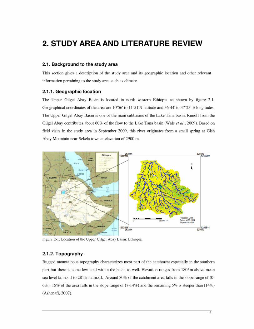
Figure 2-1: Location of the Upper Gilgel Abay Basin: Ethiopia. ...........................................................6
Figure 2-2: Cross-sectional schematization of runoff process in a sloping area at the catchment scale.
(After Rientjes, 2007). ......................................................................................................8
Figure 2-3: Expansion of saturated overland flow source areas during a storm event, (Rientjes (2007),
modified after Dunne (1978))............................................................................................9
Figure 2-4: Distribution of a , βtan and topographic index across a hill slope: (modified after
(Rientjes, 2007)).............................................................................................................10
Figure 2-5: A subsurface element as a linear storage reservoir and lateral saturated subsurface flow q
through a soil column. ....................................................................................................13
Figure 2-6: The root zone and unsaturated zone stores (Kim and Delleur, 1997). ................................16
Figure 2-7: Illustration of the routing concept (Fedak, 1999). .............................................................17
Figure 3-1: Flow chart showing sequence of the research process and methodology. ...........................25
Figure 3-2: Derivation of an estimate for the TOPMODEL m perimeter using recession curve analysis:
modified after Beven (2001). ..........................................................................................30
Figure 3-3: Illustration of concept of LAI after (after Parodi, 2002). .................................................33
Figure 3-4: Interception for agricultural crops (Von Hoyningen-Hüne, 1983; Braden, 1985) and forests
(Gash, 1979; Gash et al., 1995)......................................................................................35
Figure 3-5: Typical ranges expected in Kc for the four growth stages, (Allen et al., 1998)...................37
Figure 4-1: Vertical soil moisture profile at different places................................................................42
Figure 4-2: DEM hydroprocessing: the original DEM, the filled DEM and sink map. .........................44
Figure 4-3: Flow direction, Flow accumulation, Slope (β) and Tanβ maps. .........................................45
Figure 4-4: The Topographic Index map (left) and frequency distribution of the Topographic index
value..............................................................................................................................46
Figure 4-5: Channel routing scheme for the Gilgel Abay basin ...........................................................46
Figure 4-6: Approximate zones of influence around stations by Thiessen Polygons and the Thiessen
weights...........................................................................................................................47
Figure 4-7: Comparison of the daily rainfall: Thiessen polygon method versus the daily average rainfall.
......................................................................................................................................48
Figure 4-8: Classified landuse map of 2001 for the Upper Gilgel Abay Basin (Kebede, 2009)............49
Figure 4-9: The classified landuse maps for 1973 and 1986 (Kebede, 2009) .......................................49
Figure 4-10: Landcover types in the Upper Gilgel Abay Basin: classification by Kebede (2009). ........50
Figure 4-11: Fractional Distribution of Topographic index with Landuse. ..........................................51
Figure 5-1: Simulation results for the Upper Gilgel Abay Basin.. .......................................................52
vii
Figure 5-2: Sensitivity of the model to changes in m. ..........................................................................53
Figure 5-3: Sensitivity of model to changes in TO ...............................................................................54
Figure 5-4: Sensitivity of model to changes in ....................................................................................55
Figure 5-5: Calibration results for the Upper Gilgel Abay basin..........................................................56
Figure 5-6: Validation results for the Upper Gilgel Abay basin in 2003. .............................................57
Figure 5-7: Simulation results for different landuse classes: 1973 .......................................................59
Figure 5-8: Simulated cumulative infiltration for 1973. ......................................................................60
Figure 5-9: Comparison of observed and total simulated discharge. ....................................................61
Figure 5-10: Simulation results for different landuse classes: 1986. ....................................................61
Figure 5-11: Comparison of observed and total simulated discharge. ..................................................62
Figure 5-12: Streamflow contributions from all landuse in 2001. ........................................................63
Figure 5-13: Comparison of observed and total simulated discharge. ..................................................63
Figure 5-14: Discharge from different landuse types...........................................................................65
Figure 5-15: Maximum peakflow and annual runoff volume from different landuse types....................66
Figure 5-16: Sensitivity analysis on agricultural land..........................................................................67
viii
List of tables
Table 2-1: TOPMODEL parameter values ........................................................................................19
Table 2-2: Parameter values used in different TOPMODEL studies (Beven, 1997b) ...........................20
Table 2-3: Constant infiltration rates measured with a sprinkling infiltrometer or under rainfall.
(modified after (Dunne, 1978)). ......................................................................................22
Table 2-4: Summary table on the model approaches that are designed for landuse change impact
studies............................................................................................................................23
Table 3-1: Fieldwork Activities. .......................................................................................................26
Table 3-2: Literature values for SAVI constants and maximum LAI...................................................33
Table 3-3: A summary of the additional parameters needed for landuse analysis. ................................39
Table 3-4: Summary of how landuse/landcover is implemented in TOPMODEL and terms of the water
balance...........................................................................................................................41
Table 4-1: Frequency statistics for the soil moisture data ...................................................................43
Table 4-2: Independent T-samples test for soil moisture .....................................................................43
Table 4-3: RMSE values to validate the simple linear regression method. ...........................................47
Table 4-4: Confusion matrix for validation of land cover map of 2001: classification by Kebede (2009).
......................................................................................................................................49
Table 5-1: Parameter values used in the model. ..................................................................................52
Table 5-2: Effects of the m parameter on model efficiency. .................................................................54
Table 5-3: Effects of the TO parameter on model efficiency. ................................................................55
Table 5-4: Effects of the SRmax parameter on model efficiency. ...........................................................56
Figure 5-5: Calibration results for the Upper Gilgel Abay basin .........................................................56
Table 5-5: The accepted best parameter values and model efficiency after calibration. ........................56
Table 5-6: Parameter values obtained through calibration. .................................................................58
Table 5-7: A comparison of peak flow discharges and annual runoff volumes for different landuse. ....64
Table 5-8: Parameter values used for sensitivity analysis on agricultural land.....................................67
1
1. INTRODUCTION
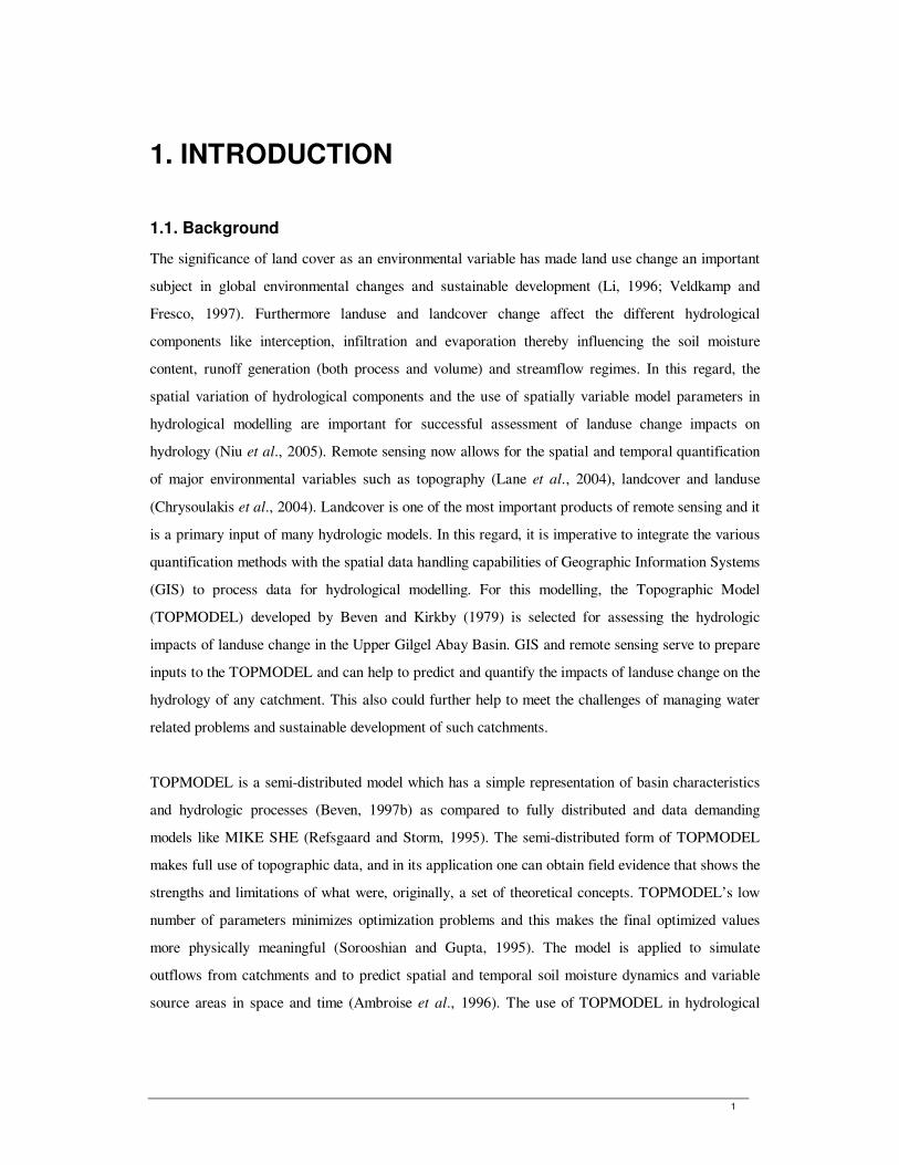
1.1. Background
The significance of land cover as an environmental variable has made land use change an important
subject in global environmental changes and sustainable development (Li, 1996; Veldkamp and
Fresco, 1997). Furthermore landuse and landcover change affect the different hydrological
components like interception, infiltration and evaporation thereby influencing the soil moisture
content, runoff generation (both process and volume) and streamflow regimes. In this regard, the
spatial variation of hydrological components and the use of spatially variable model parameters in
hydrological modelling are important for successful assessment of landuse change impacts on
hydrology (Niu et al., 2005). Remote sensing now allows for the spatial and temporal quantification
of major environmental variables such as topography (Lane et al., 2004), landcover and landuse
(Chrysoulakis et al., 2004). Landcover is one of the most important products of remote sensing and it
is a primary input of many hydrologic models. In this regard, it is imperative to integrate the various
quantification methods with the spatial data handling capabilities of Geographic Information Systems
(GIS) to process data for hydrological modelling. For this modelling, the Topographic Model
(TOPMODEL) developed by Beven and Kirkby (1979) is selected for assessing the hydrologic
impacts of landuse change in the Upper Gilgel Abay Basin. GIS and remote sensing serve to prepare
inputs to the TOPMODEL and can help to predict and quantify the impacts of landuse change on the
hydrology of any catchment. This also could further help to meet the challenges of managing water
related problems and sustainable development of such catchments.
TOPMODEL is a semi-distributed model which has a simple representation of basin characteristics
and hydrologic processes (Beven, 1997b) as compared to fully distributed and data demanding
models like MIKE SHE (Refsgaard and Storm, 1995). The semi-distributed form of TOPMODEL
makes full use of topographic data, and in its application one can obtain field evidence that shows the
strengths and limitations of what were, originally, a set of theoretical concepts. TOPMODEL’s low
number of parameters minimizes optimization problems and this makes the final optimized values
more physically meaningful (Sorooshian and Gupta, 1995). The model is applied to simulate
outflows from catchments and to predict spatial and temporal soil moisture dynamics and variable
source areas in space and time (Ambroise et al., 1996). The use of TOPMODEL in hydrological
2
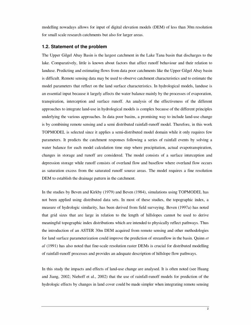
modelling nowadays allows for input of digital elevation models (DEM) of less than 30m resolution
for small scale research catchments but also for larger areas.
1.2. Statement of the problem
The Upper Gilgel Abay Basin is the largest catchment in the Lake Tana basin that discharges to the
lake. Comparatively, little is known about factors that affect runoff behaviour and their relation to
landuse. Predicting and estimating flows from data poor catchments like the Upper Gilgel Abay basin
is difficult. Remote sensing data may be used to observe catchment characteristics and to estimate the
model parameters that reflect on the land surface characteristics. In hydrological models, landuse is
an essential input because it largely affects the water balance mainly by the processes of evaporation,
transpiration, interception and surface runoff. An analysis of the effectiveness of the different
approaches to integrate land-use in hydrological models is complex because of the different principles
underlying the various approaches. In data poor basins, a promising way to include land-use change
is by combining remote sensing and a semi distributed rainfall-runoff model. Therefore, in this work
TOPMODEL is selected since it applies a semi-distributed model domain while it only requires few
parameters. It predicts the catchment responses following a series of rainfall events by solving a
water balance for each model calculation time step where precipitation, actual evapotranspiration,
changes in storage and runoff are considered. The model consists of a surface interception and
depression storage while runoff consists of overland flow and baseflow where overland flow occurs
as saturation excess from the saturated runoff source areas. The model requires a fine resolution
DEM to establish the drainage pattern in the catchment.
In the studies by Beven and Kirkby (1979) and Beven (1984), simulations using TOPMODEL has
not been applied using distributed data sets. In most of these studies, the topographic index, a
measure of hydrologic similarity, has been derived from field surveying. Beven (1997a) has noted
that grid sizes that are large in relation to the length of hillslopes cannot be used to derive
meaningful topographic index distributions which are intended to physically reflect pathways. Thus
the introduction of an ASTER 30m DEM acquired from remote sensing and other methodologies
for land surface parameterization could improve the prediction of streamflow in the basin. Quinn et
al (1991) has also noted that fine-scale resolution raster DEMs is crucial for distributed modelling
of rainfall-runoff processes and provides an adequate description of hillslope flow pathways.
In this study the impacts and effects of land-use change are analysed. It is often noted (see Huang
and Jiang, 2002; Niehoff et al., 2002) that the use of rainfall-runoff models for prediction of the
hydrologic effects by changes in land cover could be made simpler when integrating remote sensing
3
methodologies with ground based data. Thus remote sensing has been further used in this study for
the quantification of vegetation indices such as the Soil-Adjusted Vegetation Index (SAVI) and
Leaf Area Index (LAI) together with the spatial data handling capabilities of GIS. Aided with the
simplicity of the model code (Beven, 1997a), this allowed the TOPMODEL’s structure to be
changed to reflect the perceptions of the hydrological response to landuse changes in the Upper
Gilgel Abay basin..
1.3. Previous TOPMODEL studies
TOPMODEL has been successfully applied in many catchments to predict long streamflow records
and to make hydrological predictions in space and time for example for catchments in mid-Wales, see
(Quinn et al., 1991). In Beven and Freer (2000), the model has been applied where the assumption of
a quasi-steady state saturated zone configuration is replaced by a kinematic wave routing of
subsurface flow. Such is implemented in a way that allows the simulation of dynamically variable
upslope contributing areas. All this has led to significant advances in TOPMODEL simulations.
Many versions of TOPMODEL do not have an explicit parameterization of landuse, but there are
many extensions, e.g. (Famiglietti and Wood, 1995; Peters-Lidard et al., 1997), RHESSys (Band et
al., 1991) or the MACAQUE model for forests (Watson, 1999) which uses the TOPMODEL
approach for runoff estimation but extended it with a parameterization scheme for transfers of energy
between surface and atmosphere. The ITC MSc thesis work by Deginet (2008) focused on the
quantification of land surface parameters by remote sensing in the Gilgel Abay catchment but the
work did not include an analysis of how TOPMODEL can be used to assess the hydrologic impacts
of landuse changes. In addition, the improvement of TOPMODEL to handle hydrological impacts of
landuse could be a major step forward in hydrological modelling studies and to the challenges of
managing water scarcity. This work also builds on the work of Kebede (2009) who in his MSc thesis
work applied the HBV-96 model to evaluate the model response to the land cover changes for the
years 1973, 1986 and 2001. Thus the landcover maps developed in his work have been processed
further to assess the hydrological impacts of landuse on streamflow using TOPMODEL.
1.4. Objectives of the study
The main objective of this study is to assess the hydrologic impacts of landuse change in the Gilgel
Abay catchment. Further it was assessed whether the integration of remote sensing methodologies
with ground based data could improve TOPMODEL simulation results.

4
The specific objectives of this study are:
• To assess whether land surface parameterization of TOPMODEL can be achieved by use of
remote sensing.
• To evaluate how streamflow contributions from TOPMODEL can be used to initialize the model.
• To identify a suitable structure of TOPMODEL that allows for analyzing hydrologic impacts of
landuse change.
• To evaluate the streamflow contributions from different landuse classes.
• To assess the hydrological impact of landuse changes on streamflow.
• To assess sensitivity of model parameters in simulating streamflow.
The research questions are:
• Can land surface parameterization of TOPMODEL be achieved by the use of remote sensing?
• How well can TOPMODEL simulate streamflow in the catchment?
• How should the TOPMODEL structure be modified so that it can account for hydrologic
impacts of landuse change?
• What are the streamflow contributions from the different landuse classes?
• How does landuse change affect the peakflow, baseflow and runoff volume in the basin?
• How does the sum of discharge from different landuse classes compare to the observed discharge
at the outlet?
The hypotheses that follow are therefore:
• Land surface parameterization of TOPMODEL can be achieved through remote sensing.
• The model’s performance in simulating streamflow is expected to be greater than 0.7 in terms of
the Nash-Sutcliffe model’s performance.
• There is a difference in stream flow contributions from the different landuse classes.
• Landuse change has an effect on the peakflow, base flow and runoff volume.
1.5. Thesis outline
This thesis has six chapters. In the first chapter a brief background to the study is preceded by a
review of various quantification methods of landuse change on hydrologic processes with the spatial
data handling capabilities of GIS. In the same chapter the problem statement, research objectives,
research questions, research hypothesis and previous studies in the Gilgel Abay Basin are addressed.
The second chapter describes the location, topography, climate and land cover of the study area and
also discusses the various literatures this study is based on. In the third chapter, there is a discussion
of fieldwork activities, an outline of the methodology used in this study and how the TOPMODEL

5
structure can be modified to include the impacts of landuse change. Remote sensing and field data
used in this study area are described in the fourth chapter as well as the preparation of the various
input data for TOPMODEL. The chapter also explains the various analyses of the landuse data and
other related inputs to allow for application of TOPMODEL in a semi distributed fashion. Then the
fifth chapter firstly describes the results obtained and that is followed by a discussion of these results.
Chapter six contains the conclusion of this study, and finally recommendations for future studies are
made.
6
2. STUDY AREA AND LITERATURE REVIEW
2.1. Background to the study area
This section gives a description of the study area and its geographic location and other relevant
information pertaining to the study area such as climate.
2.1.1. Geographic location
The Upper Gilgel Abay Basin is located in north western Ethiopia as shown by figure 2.1.
Geographical coordinates of the area are 10º56' to 11º51'N latitude and 36º44' to 37º23' E longitudes.
The Upper Gilgel Abay Basin is one of the main subbasins of the Lake Tana basin. Runoff from the
Gilgel Abay contributes about 60% of the flow to the Lake Tana basin (Wale et al., 2009). Based on
field visits in the study area in September 2009, this river originates from a small spring at Gish
Abay Mountain near Sekela town at elevation of 2900 m.
Figure 2-1: Location of the Upper Gilgel Abay Basin: Ethiopia.
2.1.2. Topography
Rugged mountainous topography characterizes most part of the catchment especially in the southern
part but there is some low land within the basin as well. Elevation ranges from 1805m above mean
sea level (a.m.s.l) to 2811m a.m.s.l. Around 80% of the catchment area falls in the slope range of (0-
6%), 15% of the area falls in the slope range of (7-14%) and the remaining 5% is steeper than (14%)
(Ashenafi, 2007).
7
2.1.3. Climate
Ethiopia’s climate is generally affected by the Inter-Tropical Convergence Zone (ITCZ). The ITCZ
passes over Ethiopia twice a year and this migration alternatively causes the onset and withdrawals
of winds from north and south (SMEC, 2007). The Upper Gilgel Abay Basin falls within the cool
semi-humid zone with mean annual temperature of 17-20°C. The dry season occurs between
October and May while the wet season occurs mostly between June and September when the ITCZ
is to the north of the country. The climate is generally temperate at higher elevations and tropical at
the lower elevation. The long term mean annual rainfall (1992-2003) at Bahir Dar station (1828m
a.m.s.l) south of the Lake Tana is estimated to be 1416 mm. According to Wale et al., (2009), the
mean annual humidity (1994-2004) at Bahir Dar station is estimated to be 58%.
2.1.4. Soil
There are seven types of soil groups observed in this area, Alisols, Fluvisols, Leptosols, Luvisols,
Nitisols, Regosols, Vertisols (BCEOM, 1998) in combination with four diagnostic horizon
modifiers: chromic, eutric, haplic, and lithic. According to the work of BCEOM (1998), the whole
Gilgel Abay catchment is mostly covered by Haplic Luvisols with an areal coverage of around
2583 km2. The cultivated areas mostly lie on this type of soil throughout the study area. In low
lying areas particularly north of the Gilgel Abay basin, soils have been developed on alluvial
sediments (SMEC, 2007).
2.1.5. Land use and Land cover
Most of the Gilgel Abay catchment area is characterised by cropland with scarce woodlands and
forested highlands. The main croplands as observed during a field visit consist of maize, turf and
potato. Besides the cultivated lands, the main landcover types are grassland, marshland, and forest
with frequent patches of shrubs, eucalyptus woods and trees. According to a landcover
classification of 2001 done by Kebede (2009), the major land cover types include 62%, agriculture,
17% forests, 11.6% shrub land, 9% grassland, and 0.4% water and marshy lands. Agricultural
production is very low because of the shortage of skilled manpower, backward technology, poor
infrastructure in rural Ethiopia, recurrent drought, and land degradation. Land degradation is
perhaps the most significant factor (Tessema, 2006 ).
8
2.2. Literature review: Topmodel approach
This section describes the dominant runoff processes occurring at the hillslope, the concept of
TOPMODEL, the governing equations and how TOPMODEL solves the water balance for a
catchment.
2.2.1. Dominant flow processes at the hillslope
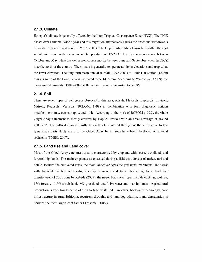
There are many processes that contribute to catchment runoff at the catchment outlet point. Figure
2-2 shows a schematic representation of flow processes which may contribute to the catchment
runoff.
Figure 2-2: Cross-sectional schematization of runoff process in a sloping area at the catchment scale. (After
Rientjes, 2007).
Hortonian overland flow (infiltration excess overland flow) occurs when rainfall intensity exceeds
the infiltration capacity of the soil. This may occur at any location in a catchment and is common
in arid climates and in low permeable areas e.g. urbanized areas. In contrast, saturation overland
flow occurs when the soil is saturated due to a rise of the phreatic groundwater level. This process
is much less aggressive compared to Hortonian overland flow and is common in lower parts of the
catchment. On top of these saturated zones, overland flow is generated by exfiltration of
subsurface water and by rainfall. These zones are termed the ‘saturation overland flow source
areas’ and are shown in figure 2-3. Unsaturated subsurface flow is the flow of water in a matrix
flow system where the movement of water is due to suction head gradients. Infiltration of rainfall
in the subsurface can be in the form of matrix flow or macro pore flow (or small natural pipes). A
matrix flow system is often discontinuous due to macro pores as caused by (drought) cracks,
wormholes or rooting of vegetation. Perched subsurface flow is generated when the saturated
hydraulic conductivity of a given subsurface layer is significantly lower than the overlaying soil
layer. Groundwater flow is the flow of water in the saturated zone. The groundwater system acts as
a storage reservoir for base flow generation. Groundwater flow contributions can be ‘rapid’ and
9
‘delayed’. When water reaches the natural or artificial catchment drainage system, water is
transported through the main channels. Finally in the channel system, runoff contributions from the
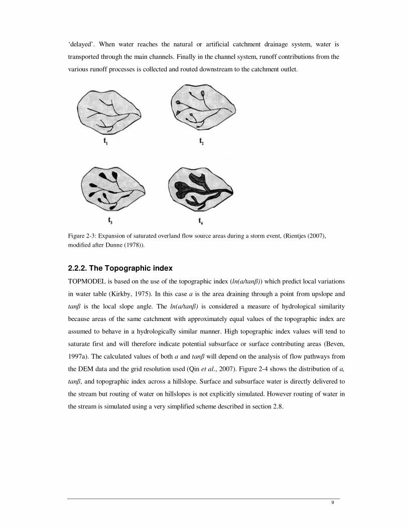
various runoff processes is collected and routed downstream to the catchment outlet.
Figure 2-3: Expansion of saturated overland flow source areas during a storm event, (Rientjes (2007),
modified after Dunne (1978)).
2.2.2. The Topographic index
TOPMODEL is based on the use of the topographic index (ln(a/tanβ)) which predict local variations
in water table (Kirkby, 1975). In this case a is the area draining through a point from upslope and
tanβ is the local slope angle. The ln(a/tanβ) is considered a measure of hydrological similarity
because areas of the same catchment with approximately equal values of the topographic index are
assumed to behave in a hydrologically similar manner. High topographic index values will tend to
saturate first and will therefore indicate potential subsurface or surface contributing areas (Beven,
1997a). The calculated values of both a and tanβ will depend on the analysis of flow pathways from
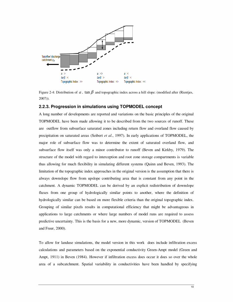
the DEM data and the grid resolution used (Qin et al., 2007). Figure 2-4 shows the distribution of a,
tanβ, and topographic index across a hillslope. Surface and subsurface water is directly delivered to
the stream but routing of water on hillslopes is not explicitly simulated. However routing of water in
the stream is simulated using a very simplified scheme described in section 2.8.
10
Figure 2-4: Distribution of a , βtan and topographic index across a hill slope: (modified after (Rientjes,
2007)).
2.2.3. Progression in simulations using TOPMODEL concept
A long number of developments are reported and variations on the basic principles of the original
TOPMODEL have been made allowing it to be described from the two sources of runoff. These
are outflow from subsurface saturated zones including return flow and overland flow caused by
precipitation on saturated areas (Seibert et al., 1997). In early applications of TOPMODEL, the
major role of subsurface flow was to determine the extent of saturated overland flow, and
subsurface flow itself was only a minor contributor to runoff (Beven and Kirkby, 1979). The
structure of the model with regard to interception and root zone storage compartments is variable
thus allowing for much flexibility in simulating different systems (Quinn and Beven, 1993). The
limitation of the topographic index approaches in the original version is the assumption that there is
always downslope flow from upslope contributing area that is constant from any point in the
catchment. A dynamic TOPMODEL can be derived by an explicit redistribution of downslope
fluxes from one group of hydrologically similar points to another, where the definition of
hydrologically similar can be based on more flexible criteria than the original topographic index.
Grouping of similar pixels results in computational efficiency that might be advantageous in
applications to large catchments or where large numbers of model runs are required to assess
predictive uncertainty. This is the basis for a new, more dynamic, version of TOPMODEL (Beven
and Freer, 2000).
To allow for landuse simulations, the model version in this work does include infiltration excess
calculations and parameters based on the exponential conductivity Green-Ampt model (Green and
Ampt, 1911) in Beven (1984). However if infiltration excess does occur it does so over the whole
area of a subcatchment. Spatial variability in conductivities have been handled by specifying

11
different saturated hydraulic conductivity (Ks) parameter values for different subcatchments, even if
they have the same ln(a/tanβ) and routing parameters, i.e. to represent different fractions of the same
catchment area.
2.2.4. Assumptions of TOPMODEL
In summary, TOPMODEL is based on the assumption that local soil moisture dynamics strongly
depends on the size of the upslope area (a) that drains through an observed catchment point, the
local surface topographic slope (tan ß) that represents the hydraulic gradient for saturated water
flow, and the downslope soil transmissivity (To).
The four underlying assumptions are:
(i) Dynamics of the saturated zone can be approximated by successive steady state
representations
(ii) Hydraulic gradient of the saturated zone can be approximated by the local surface topographic
slope
(iii) Transmissivity with depth is an exponential function of the storage deficit or the depth to the
water table.
(iv) Saturation of the soil column occurs from below and as such runoff generated by the saturation
excess overland flow mechanism.
2.2.5. Description of the model and governing equations
For this study a code of the model approach has been developed using the IDL programming
language. Equations and algorithms of the code are by Beven (1997) and Beven (2001). The lecture
notes by Rientjes (2007) and the MSc thesis by Pilot (2002) have also been used for explanation of
these equations. The essential concepts of TOPMODEL are primarily concerned with a simplified
model of the saturated zone and its control of surface and subsurface contributing areas. However, to
complete a continuous simulation model it is necessary to introduce further components to deal with
interception, infiltration, evapotranspiration, the unsaturated zone and flow routing (Beven, 1997a).
2.2.6. What happens in the saturated zone?
The TOPMODEL approach is based on the storage principle and applies a Darcy type flow equation
to allow water transport between subsurface storage elements. This equation is not solved
numerically where hydraulic heads are updated per calculations time step but topographic gradients
serve as fixed hydraulic gradients to simulate mass transfer (Rientjes, 2007). One of the parameters
in the Darcy equation is Transmissivity that is equal to the depth of the flow domain as multiplied by
the hydraulic conductivity. Since groundwater flow only is possible in the saturated zone,
12
transmissivity must be calculated for that part of the subsurface that is fully saturated and any cross
sectional flow area for groundwater flow is a function of the depth of the saturated zone (Pilot,
2002).
fz
oeTT−= or ∫
∞− ==
0 f
kdzekT ofz
o [1]
Where:
To = the transmissivity at the surface (lateral transmissivity), [L2T
-1]
z = local water table depth, [L]
f = a scaling parameter [L-1
]
The distribution of transmissivity in downslope direction can be simulated by an exponential function
of the local storage deficit. This deficit refers to the amount of water to reach full saturation of the
soil column Similarly, the decline of local transmissivity with decreasing storage in the soil profile
has been approximated by an exponential function (Quinn et al., 1995).
ms
oieTT
−= [2]
Where:
Si = current local saturated zone storage deficit,
m = parameter controlling the shape of the function.
If the soil saturation reaches its maximum (i.e. deficit becomes zero), the lateral discharge becomes
maximum. The saturated zone is recharged by rainwater although important processes such as
infiltration and unsaturated flow zone are ignored.
Subsurface flow
If S represents the storage deficit, the maximum discharge in the subsurface is observed when the
entire soil profile becomes saturated and discharge is equal to:
TSq =max [3]
The actual groundwater discharge is a function of the upstream area ‘a’ as multiplied by the recharge
rate ‘R’
Raqact = [4]
Where:
qact = actual lateral discharge [m/hr] [L2T
-1]
R = recharge rate or proportionality constant [LT-1
]
a = specific catchment area [L]
13
The proportionality constant in TOPMODEL approach may be interpreted as “steady state” recharge
rate, or “steady state” per unit area contribution to base flow (Rientjes, 2007). When comparing the
actual discharge to the maximum discharge an indication is obtained towards the “relative wetness”
‘w’ or saturation degree of the subsurface grid cell that represents the real world soil column (Dunne,
1978). The relative wetness describes the ratio of actual discharge and maximum discharge and may
be interpreted as available storage depth to reach full saturation in the saturated subsurface:
i
act
TS
Ra
q
qw ==
max
[5]
Full saturation occurs when the wetness becomes larger than 1 or when following equation [5]:
RBT
a 1
tan> [6]
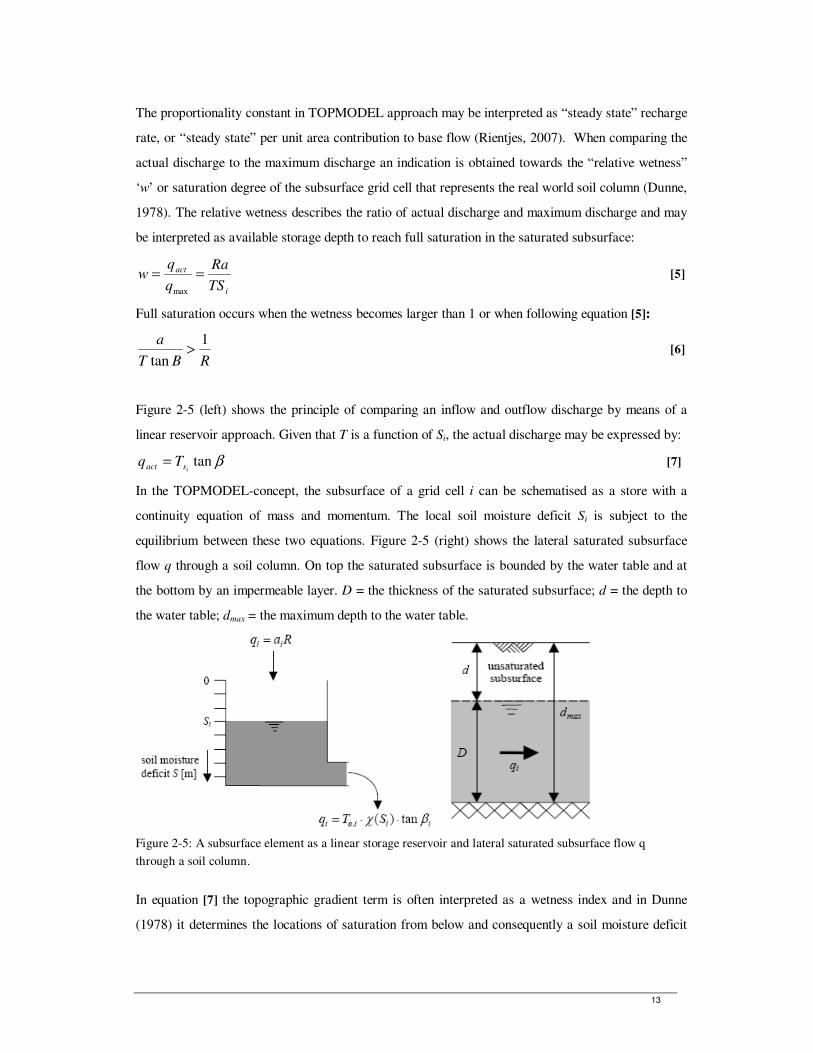
Figure 2-5 (left) shows the principle of comparing an inflow and outflow discharge by means of a
linear reservoir approach. Given that T is a function of Si, the actual discharge may be expressed by:
βtanisact Tq = [7]
In the TOPMODEL-concept, the subsurface of a grid cell i can be schematised as a store with a
continuity equation of mass and momentum. The local soil moisture deficit Si is subject to the
equilibrium between these two equations. Figure 2-5 (right) shows the lateral saturated subsurface
flow q through a soil column. On top the saturated subsurface is bounded by the water table and at
the bottom by an impermeable layer. D = the thickness of the saturated subsurface; d = the depth to
the water table; dmax = the maximum depth to the water table.
Figure 2-5: A subsurface element as a linear storage reservoir and lateral saturated subsurface flow q
through a soil column.
In equation [7] the topographic gradient term is often interpreted as a wetness index and in Dunne
(1978) it determines the locations of saturation from below and consequently a soil moisture deficit

14
may occur. When T is assumed to be fixed property because K is uniformly distributed and D is
finite, then:
ββ tantan
a
T
a= or
βtanln
a [8]
The relative wetness becomes:
βtan
Raw = [9]
If the hydraulic conductivity is uniformly distributed and assuming that the depth of the soil column
is finite:
∫
==
daaA
aw
T
Raw
β
β
βtan
1
tan
tan [10]
If the ‘unsaturated zone” thickness is simulated it becomes:
)1( wDz −= [11]
When the exponential K assumption that describes the saturated hydraulic conductivity is introduced
then the transmissivity reduces exponentially (equation [11]), and:
ifz
o eTaR−= βtan [12]
With the same logic of equation [s], the local soil deficit can be expressed by:
−−=
−= λ
ββ tanln
1
tanln
1 a
fz
T
Ra
fz i [13]
When the local deficit over the entire catchment is integrated to give a mean depth z to the water
table gives:
dARa
fAdAz
Az
AA
i ∫∫
−
−== ln
tanln
11
β [14]
Now equation [11] is assumed to hold for water table rising above the soil surface. When rewriting
equation [12] and when substituting this for R in equation [14], R is eliminated and z becomes a
function of topographic and physiographic properties only:
++
−= ∫ ββ tan
lntan
ln11
o
i
A o T
afzdA
T
a
Afz [15]
or

15
}{ aoi TTa
zzf lnlntan
ln)( −−
−
=− λ
β [16]
Where:
dAa
A ∫
=
βλ
tanln
1
dATA
TA ∫= ln1
ln
The equation expresses the deviation of the local depth of the water table scaled to parameter ‘f’ in
terms of the deviation in the logarithm of transmissivity away from the integral value Ln TA and a
deviation in the local topographic index away from its integral value λ, the catchment topographic
constant as described (Beven and Kirkby, 1979).
Rewriting equation [15] for zi gives:
−= λ
βtanln
1 a
fzz i
Where:
+−=
T
R
fz ln
1λ
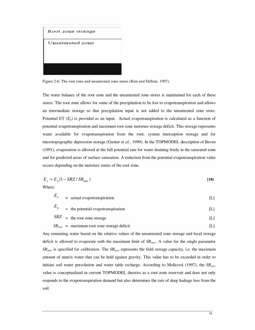
2.2.7. What happens in the unsaturated zone and root zone reservoir?
Figure 2-6 shows a schematic structure of the root zone storage and unsaturated zone. The vertical
drainage from the unsaturated zone to the saturated zone as suggested by Beven and Wood (1983) is
given by the following equation:
di
uz
vtS
Sq = [17]
Where:
qv = the vertical (gravity) drainage from the unsaturated zone [LT-1
]
uzS = the unsaturated zone storage [L]
iS = local saturated zone deficit [L]
td = time delay constant of the unsaturated zone [T]
16
Figure 2-6: The root zone and unsaturated zone stores (Kim and Delleur, 1997).
The water balance of the root zone and the unsaturated zone stores is maintained for each of these
stores. The root zone allows for some of the precipitation to be lost to evapotranspiration and allows
an intermediate storage so that precipitation input is not added to the unsaturated zone store.
Potential ET (Ep) is provided as an input. Actual evapotranspiration is calculated as a function of
potential evapotranspiration and maximum root zone moisture storage deficit. This storage represents
water available for evapotranspiration from the root, system interception storage and for
microtopographic depression storage (Gunter et al., 1999). In the TOPMODEL description of Beven
(1991), evaporation is allowed at the full potential rate for water draining freely in the saturated zone
and for predicted areas of surface saturation. A reduction from the potential evapotranspiration value
occurs depending on the moisture status of the root zone.
)/1( maxSRSRZEE pa −= [18]
Where:
aE = actual evapotranspiration [L]
pE = the potential evapotranspiration [L]
SRZ = the root zone storage [L]
SRmax = maximum root zone storage deficit [L]
Any remaining water based on the relative values of the unsaturated zone storage and local storage
deficit is allowed to evaporate with the maximum limit of SRmax. A value for the single parameter
SRmax is specified for calibration. The SRmax represents the field storage capacity, i.e. the maximum
amount of matrix water that can be held against gravity. This value has to be exceeded in order to
initiate soil water percolation and water table recharge. According to Molicová (1997), the SRmax
value is conceptualized in current TOPMODEL theories as a root zone reservoir and does not only
responds to the evapotranspiration demand but also determines the rate of deep leakage loss from the
soil.
17
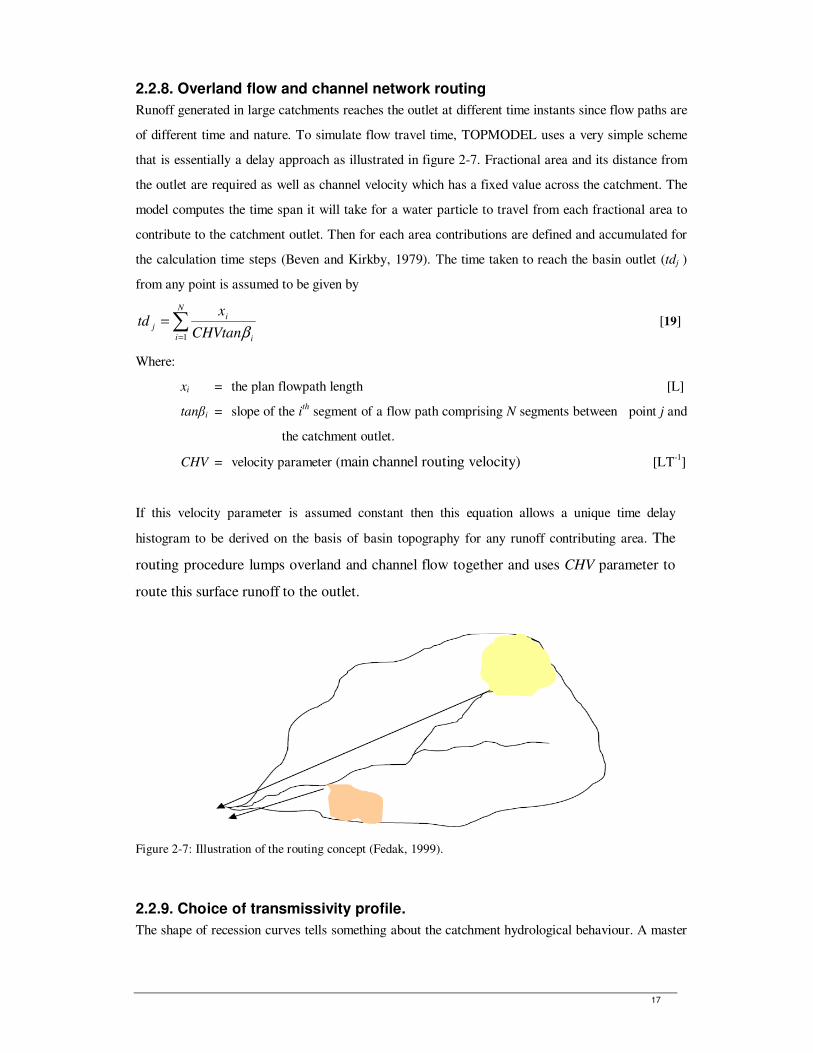
2.2.8. Overland flow and channel network routing
Runoff generated in large catchments reaches the outlet at different time instants since flow paths are
of different time and nature. To simulate flow travel time, TOPMODEL uses a very simple scheme
that is essentially a delay approach as illustrated in figure 2-7. Fractional area and its distance from
the outlet are required as well as channel velocity which has a fixed value across the catchment. The
model computes the time span it will take for a water particle to travel from each fractional area to
contribute to the catchment outlet. Then for each area contributions are defined and accumulated for
the calculation time steps (Beven and Kirkby, 1979). The time taken to reach the basin outlet (tdj )
from any point is assumed to be given by
∑=
=N
i i
i
jHVtanC
xtd
1 β [19]
Where:
xi = the plan flowpath length [L]
tanβi = slope of the ith
segment of a flow path comprising N segments between point j and
the catchment outlet.
CHV = velocity parameter (main channel routing velocity) [LT-1
]
If this velocity parameter is assumed constant then this equation allows a unique time delay
histogram to be derived on the basis of basin topography for any runoff contributing area. The
routing procedure lumps overland and channel flow together and uses CHV parameter to
route this surface runoff to the outlet.
Figure 2-7: Illustration of the routing concept (Fedak, 1999).
2.2.9. Choice of transmissivity profile.
The shape of recession curves tells something about the catchment hydrological behaviour. A master
18
recession curve is an artificial curve but is made of a collection of measured single recession curves
(Pilot, 2002). It describes the depletion of the catchment area in time from the highest measured peak
discharge to the smallest measured amount of outflow. With the master recession curve, the
parameters of the TOPMODEL-concept can be derived. To start with a relative local soil moisture
deficit, δi is defined:
Exponential Parabolic Linear
ii mS δ= ii mS δ= ii mS δ= [20]
Where:
Si = local soil moisture deficit [m]
Sm = maximum soil moisture deficit [m]
m = rate of exponential decrease of Ti with Si [m]
δi = relative local storage deficit [-]
The momentum equations are given as:
Exponential Parabolic Linear
iioi taneTq i βδ−= , iiioi tanTq βδ 2
, )1( −= iiioi tanTq βδ )1(, −= [21]
Within this newly obtained equation the soil moisture deficit is the hydrologic state variable:
Exponential Parabolic Linear
iioi taneTq i βδ−= , iiioi tanTRa βδ 2
, )1( −= iiioi tanTRa βδ )1(, −= [22]
Representation of the recession curve within the TOPMODEL-concept
For the situation of a base flow recession period (a period of drainage without recharge), Ambroise et
al.,(1996) proposed a procedure on how to determine the transmissivity profile that is corresponding
to the involved catchment. If Qb is the discharge at the catchment outlet [m3/d] and Qo is the
discharge of the base flow in case δ = 0 [m3/d] then the relation between Qb and δ can be written for
Qb as a function of time. In case the mean relative storage deficit δ= 0 and thus Qb =Qo, the
corresponding stored volume of groundwater, Vo, in the catchment is:
Exponential Parabolic Linear
∞=Vo mASVo = mASVo = [23]
It is assumed that there is no lower limit in the exponential transmissivity profile. In the period of
drainage without recharge, the conservation equation reads:
19
dt
dASQ mb
δ= [24]
The general differential equation that describes the decrease of the outflow with time in the base flow
recession curve is:
δd
dQ
AS
Q
dt
dQ b
m
bb = [25]
with Sm = m in case of the exponential transmissivity profile.
The base flow recession curve can be written for Qb at t = ts + τ. with any specified discharge Qs at t
= ts:
Exponential Parabolic Linear
τAm
Q
s
s
b 11+
= 2
1
+
=
τm
o
s
s
b
AS
−= τ
m
o
sbAS
QeQQ [26]
first order hyperbolic second order hyperbolic exponential
Equation [26] gives the expressions for the base flow recession curve for each of the three defined
transmissivity profiles. For the exponential transmissivity profile, this results in a first order
hyperbolic recession curve, for the parabolic profile in a second order hyperbolic curve and assuming
a linear transmissivity profile results in an exponential base flow recession curve.
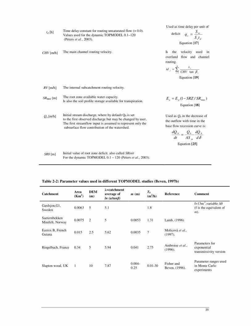
2.2.10. TOPMODEL parameters
The version of TOPMODEL used in this study has 8 parameters that are described in Table 2-1.
Table 2-1: TOPMODEL parameter values
Parameter Meaning/definition Where parameter is used
m [m] Parameter of the exponential transmissivity function or
recession curve.
Controls rate of decline of To.
Derived from an analysis of catchment recession curves.
A plot on vertical axes (1/discharge) and on horizontal axes
(time in hours) graph (Beven et al., 1995). Lower limit 0.005.
Use in the equation of decline
of local transmissivity with
decreasing storage in the soil
profile. (Quinn et al., 1995). ms
oieTT
−=
Equation [2]
To [m2/h] Average transmissivity of the soil when the profile is just
saturated. A homogeneous soil throughout the catchment is
assumed. Published values include 35 for a 60 m grid cell
&42 for 20m grid cell size (Saulnier et al.1997).
ms
oieTT
−=
Equation [2]
20
td [h]
Time delay constant for routing unsaturated flow (> 0.0).
Values used for the dynamic TOPMODEL 0.1–120
(Peters et al., 2003).
Used as time delay per unit of
deficit
di
uz
vtS
Sq =
Equation [17]
CHV [m/h]
The main channel routing velocity.
Is the velocity used in
overland flow and channel
routing.
∑=
=N
i i
i
jCHV
xtd
1 tan β
Equation [19]
RV [m/h]
The internal subcatchment routing velocity.
SRmax [m]
The root zone available water capacity.
Is also the soil profile storage available for transpiration.
)/1( maxSRSRZEE pa −=
Equation [18]
Qo [m/h]
Initial stream discharge, where by default Q0 is set
to the first observed discharge but may be changed by user,
The first streamflow input is assumed to represent only the
subsurface flow contribution of the watershed.
Used as Qb in the decrease of
the outflow with time in the
base flow recession curve is:
δd
dQ
AS
Q
dt
dQ b
m
bb =
Equation [25]
SR0 [m]
Initial value of root zone deficit. also called SRinit
For the dynamic TOPMODEL 0.1 – 120 (Peters et al., 2003).
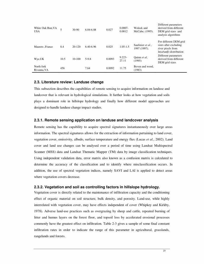
Table 2-2: Parameter values used in different TOPMODEL studies (Beven, 1997b)
Catchment Area
(Km2)
DEM
(m)
λ=catchment
average of
ln (a/tanβ)
m (m) T0
(m2/h) Reference Comment
Gardsjon,G1,
Sweden 0.0063 5 5.1 1.8
f=13m-1,variable ∆θ
(f is the equivalent of
m).
Saeternbekken
Minifelt, Norway 0.0075 2 5 0.0053 1.31 Lamb, (1996)
Ecerex B, French
Guiana 0.015 2.5 5.62 0.0035 7
Molicová et al.,
(1997).
Ringelbach, France 0.34 5 5.94 0.041 2.75 Ambroise et al.,
(1996).
Parameters for
exponential
transmissivity version
Slapton wood, UK 1 10 7.87 0.004-
0.25 0.01-30
Fisher and
Beven, (1996).
Parameter ranges used
in Monte Carlo
experiments
21
White Oak Run,VA
USA 5 30-90 6.04-6.08 0.027
0.0007-
0.0012
Wolock and
McCabe, (1995).
Different parameters
derived from different
DEM grid sizes and
analysis algorithms
Maurets ,France 8.4 20-120 6.40-6.96 0.025 1.05-1.5 Saulinier et al.,
1997 (1997).
For different DEM grid
sizes after excluding
river pixels from
ln(a/tanβ) distribution
Wye,UK 10.5 10-100 5-9.8 0.0093 9.223-
27.11
Quinn et al,
(1995)
Different parameters
derived from different
DEM grid sizes
North fork
Rivanna,VA 456 7.64 0.0092 11.75
Beven and wood,
(1983)
2.3. Literature review: Landuse change
This subsection describes the capabilities of remote sensing to acquire information on landuse and
landcover that is relevant in hydrological simulations. It further looks at how vegetation and soils
plays a dominant role in hillslope hydrology and finally how different model approaches are
designed to handle landuse change impact studies.
2.3.1. Remote sensing application on landuse and landcover analysis
Remote sensing has the capability to acquire spectral signatures instantaneously over large areas
information. The spectral signatures allows for the extraction of information pertaining to land cover,
vegetation cover, emissivity, albedo, surface temperature and energy flux (Lucas et al., 2002). Land
cover and land use changes can be analysed over a period of time using Landsat Multispectral
Scanner (MSS) data and Landsat Thematic Mapper (TM) data by image classification techniques.
Using independent validation data, error matrix also known as a confusion matrix is calculated to
determine the accuracy of the classification and to identify where misclassification occurs. In
addition, the use of spectral vegetation indices, namely SAVI and LAI is applied to detect areas
where vegetation covers decrease.
2.3.2. Vegetation and soil as controlling factors in hillslope hydrology.
Vegetation cover is directly related to the maintenance of infiltration capacity and the conditioning
effect of organic material on soil structure, bulk density, and porosity. Land-use, while highly
interrelated with vegetation cover, may have effects independent of cover (Whipkey and Kirkby,
1978). Adverse land-use practices such as overgrazing by sheep and cattle, repeated burning of
litter and humus layers on the forest floor, and topsoil loss by accelerated erosional processes
commonly have the greatest effect on infiltration. Table 2-3 gives a sample of some final constant
infiltration rates in order to indicate the range of this parameter in agricultural, grasslands,
rangelands and forests.
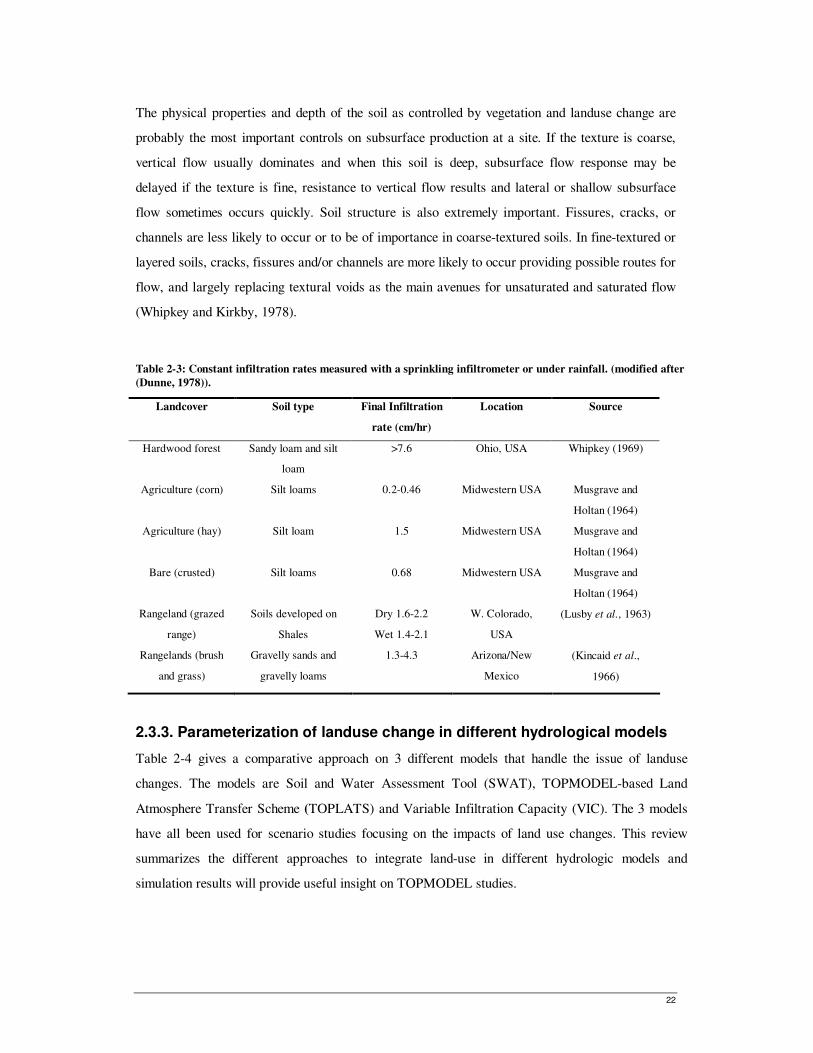
22
The physical properties and depth of the soil as controlled by vegetation and landuse change are
probably the most important controls on subsurface production at a site. If the texture is coarse,
vertical flow usually dominates and when this soil is deep, subsurface flow response may be
delayed if the texture is fine, resistance to vertical flow results and lateral or shallow subsurface
flow sometimes occurs quickly. Soil structure is also extremely important. Fissures, cracks, or
channels are less likely to occur or to be of importance in coarse-textured soils. In fine-textured or
layered soils, cracks, fissures and/or channels are more likely to occur providing possible routes for
flow, and largely replacing textural voids as the main avenues for unsaturated and saturated flow
(Whipkey and Kirkby, 1978).
Table 2-3: Constant infiltration rates measured with a sprinkling infiltrometer or under rainfall. (modified after
(Dunne, 1978)).
Landcover Soil type Final Infiltration
rate (cm/hr)
Location Source
Hardwood forest Sandy loam and silt
loam
>7.6 Ohio, USA Whipkey (1969)
Agriculture (corn) Silt loams 0.2-0.46 Midwestern USA Musgrave and
Holtan (1964)
Agriculture (hay) Silt loam 1.5 Midwestern USA Musgrave and
Holtan (1964)
Bare (crusted) Silt loams 0.68 Midwestern USA Musgrave and
Holtan (1964)
Rangeland (grazed
range)
Soils developed on
Shales
Dry 1.6-2.2
Wet 1.4-2.1
W. Colorado,
USA
(Lusby et al., 1963)
Rangelands (brush
and grass)
Gravelly sands and
gravelly loams
1.3-4.3 Arizona/New
Mexico
(Kincaid et al.,
1966)
2.3.3. Parameterization of landuse change in different hydrological models
Table 2-4 gives a comparative approach on 3 different models that handle the issue of landuse
changes. The models are Soil and Water Assessment Tool (SWAT), TOPMODEL-based Land
Atmosphere Transfer Scheme (TOPLATS) and Variable Infiltration Capacity (VIC). The 3 models
have all been used for scenario studies focusing on the impacts of land use changes. This review
summarizes the different approaches to integrate land-use in different hydrologic models and
simulation results will provide useful insight on TOPMODEL studies.
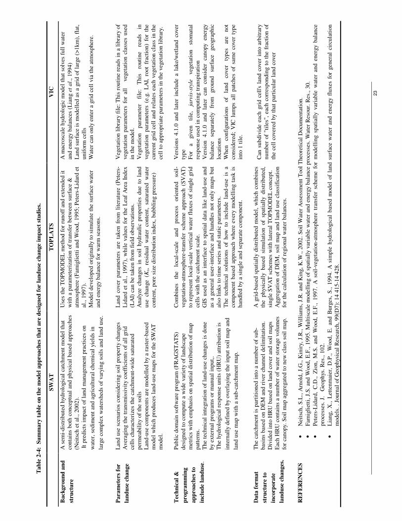
23
Ta
ble
2-4
: S
um
mary
tab
le o
n t
he
mod
el a
pp
roach
es t
hat
are
des
ign
ed f
or
lan
du
se c
ha
nge
imp
act
stu
die
s.
S
WA
T
TO
PL
AT
S
VIC
Ba
ckg
rou
nd
an
d
stru
ctu
re
A s
emi-
dis
trib
ute
d h
ydro
logic
al c
atch
men
t m
odel
that
conta
ins
both
conce
ptu
al a
nd p
hys
ical
bas
ed a
ppro
aches
(Nei
tsch
et
al.,
2002
).
It
pre
dic
ts i
mp
act
of
land m
anag
emen
t p
ract
ices
on
wat
er,
sedim
ent
and
agri
cult
ura
l ch
emic
al y
ield
s in
larg
e co
mple
x w
ater
shed
s of
var
ying s
oil
s an
d l
and u
se.
Use
s th
e T
OP
MO
DE
L m
ethod f
or
runoff
and e
xte
nded
it
wit
h a
par
amet
eriz
atio
n o
f tr
ansf
er b
etw
een s
urf
ace
&
atm
osp
her
e (F
amig
liet
ti a
nd W
ood
, 1995;
Pet
ers-
Lid
ard e
t
al.,
1997).
Model
dev
eloped
ori
gin
ally
to s
imula
te t
he
surf
ace
wat
er
and e
ner
gy
bal
ance
for
war
m s
easo
ns.
A m
acro
scal
e hyd
rolo
gic
model
that
solv
es f
ull
wat
er
and e
ner
gy
bal
ance
s (L
iang e
t al.
, 1994)
Lan
d s
urf
ace
is m
odel
led
as
a gri
d o
f la
rge
(>1km
), f
lat,
un
iform
cel
ls
Wat
er c
an o
nly
ente
r a
gri
d c
ell
via
the
atm
osp
her
e.
Pa
ram
eter
s fo
r
lan
du
se c
ha
ng
e
Lan
d u
se s
cenar
ios
consi
der
ing s
oil
pro
per
ty c
han
ges
Aver
agin
g t
he
tran
smis
sivit
y co
effi
cien
ts o
f al
l gri
d
cell
s ch
arac
teri
zes
the
catc
hm
ent-
wid
e sa
tura
ted
per
mea
bil
ity
of
the
soil
s
Lan
d-u
se c
om
ponen
ts a
re m
odel
led b
y a
rast
er-b
ased
mod
el w
hic
h p
roduce
s la
nd-u
se m
aps
for
the
SW
AT
mod
el.
Lan
d c
over
par
amet
ers
are
taken
fro
m l
iter
ature
(P
eter
s-
Lid
ard e
t al
., 1
997),
whil
e val
ues
for
the
Lea
f A
rea
Index
(LA
I) c
an b
e ta
ken
fro
m f
ield
obse
rvat
ions.
Anal
yze
chan
ges
in s
oil
hyd
rauli
c pro
per
ties
due
to l
and
use
ch
ange
(Ks,
re
sid
ual
w
ater
co
nte
nt,
sa
tura
ted
w
ater
conte
nt,
pore
siz
e dis
trib
uti
on i
ndex
, bubbli
ng p
ress
ure
)
Veg
etat
ion l
ibra
ry f
ile:
This
routi
ne
read
s in
a l
ibra
ry o
f
veg
etat
ion p
aram
eter
s fo
r al
l
veg
etat
ion c
lass
es u
sed
in t
he
model
.
Veg
etat
ion
par
amet
er
file
: T
his
ro
uti
ne
read
s in
veg
etat
ion p
aram
eter
s (e
.g.
LA
I, r
oot
frac
tion)
for
the
curr
ent
gri
d c
ell
and r
elat
es e
ach v
eget
atio
n c
lass
in t
he
cell
to a
ppro
pri
ate
par
amet
ers
in t
he
veg
etat
ion l
ibra
ry.
Tec
hn
ica
l &
pro
gra
mm
ing
ap
pro
ach
es t
o
incl
ud
e la
nd
use
.
Publi
c dom
ain
soft
war
e pro
gra
m (
FR
AG
ST
AT
S)
des
igned
to c
om
pute
a w
ide
var
iety
of
landsc
ape
met
rics
wit
h e
mphas
is o
n s
pat
ial
dis
trib
uti
on o
f m
ap
pat
tern
s.
The
tech
nic
al i
nte
gra
tion o
f la
nd
-use
chan
ges
is
done
by
exte
rnal
pro
gra
ms
or
man
ual
input,
.
The
hyd
rolo
gic
al r
esponse
unit
s (H
RU
) at
trib
uti
on i
s
inte
rnal
ly d
efin
ed b
y over
layi
ng t
he
inpu
t so
il m
ap a
nd
land
use
map
wit
h a
sub-c
atch
men
t m
ap.
Com
bin
es
the
loca
l-sc
ale
and
pro
cess
ori
ente
d
soil
-
veg
etat
ion-a
tmosp
her
e-tr
ansf
er s
chem
e ap
pro
ach (
SV
AT
)
to r
epre
sen
t lo
cal-
scal
e ver
tica
l w
ater
flu
xes
of
single
gri
d
cell
s w
ith t
he
catc
hm
ent
scal
e.
GIS
use
d a
s an
inte
rfac
e to
spat
ial
dat
a li
ke
land-u
se a
nd
as a
gen
eral
use
r-in
terf
ace
and h
andle
s not
on
ly m
aps
but
also
lin
ks
to t
ime
seri
es a
nd s
tati
c par
amet
ers.
The
tech
nic
al s
olu
tion
s of
how
to i
ncl
ude
land-u
se i
s a
com
ponen
t bas
ed a
ppro
ach w
her
e ev
ery
mod
elli
ng t
ask i
s
han
dle
d b
y a
single
an
d s
epar
ate
com
ponen
t.
Ver
sions
4.1
.0 a
nd l
ater
incl
ude
a la
ke/
wet
lan
d c
over
type
For
a giv
en
tile
, ja
rvis
-sty
le
veg
etat
ion
stom
atal
resp
onse
use
d i
n c
om
puti
ng t
ransp
irat
ion
Ver
sion
4.1
.0
and
late
r ca
n
consi
der
ca
nopy
ener
gy
bal
ance
se
par
atel
y fr
om
gro
und
surf
ace
geo
gra
phic
loca
tions
When
co
nfi
gura
tions
of
land
cover
ty
pes
ar
e not
consi
der
ed;
VIC
lum
ps
all
pat
ches
of
sam
e co
ver
typ
e
into
1 t
ile.
Da
ta f
orm
at
stru
ctu
re t
o
inco
rpora
te
lan
du
se c
ha
ng
es.
The
catc
hm
ent
is p
arti
tion
ed i
nto
a n
um
ber
of
sub-
bas
ins
bas
ed o
n D
EM
and
riv
er c
han
nel
del
imit
atio
n.
Div
ided
into
HR
U b
ased
on l
and
cover
and s
oil
map
s
Eac
h H
RU
con
tain
s a
num
ber
of
wat
er s
tora
ge
volu
mes
for
canop
y. S
oil
map
aggre
gat
ed t
o n
ew c
lass
soil
map
.
A g
rid-b
ased
spat
iall
y dis
trib
ute
d m
odel
, w
hic
h c
om
bin
es
the
phys
ical
ly bas
ed
sim
ula
tion of
spat
iall
y dis
trib
ute
d,
single
SV
AT
sch
emes
wit
h l
ater
al T
OP
MO
DE
L c
on
cept.
Aggre
gat
ion o
f D
EM
, so
il m
ap a
nd l
and u
se c
lass
ific
atio
n
for
the
calc
ula
tion o
f re
gio
nal
wat
er b
alan
ces.
Can
subdiv
ide
each
gri
d c
ell's
lan
d c
over
into
arb
itra
ry
nu
mber
of
"til
es",
eac
h c
orr
espondin
g t
o t
he
frac
tion o
f
the
cell
cover
ed b
y th
at p
arti
cula
r la
nd c
over
RE
FE
RE
NC
ES
•
Nei
tsch
, S
.L.,
Arn
old
, J.
G.,
Kin
iry,
J.R
., W
illi
ams,
J.R
. an
d K
ing,
K.W
., 2
002.
Soil
Wat
er A
sses
smen
t T
ool
Theo
reti
cal
Docu
men
tati
on
.
• F
amig
liet
ti,
J.S
. an
d W
ood,
E.F
., 1
99
5.
Mult
isca
le m
odel
lin
g o
f sp
atia
lly
var
iable
wat
er a
nd e
ner
gy
bal
ance
pro
cess
es.
Wat
er R
esour.
Res
., 3
0.
• P
eter
s-L
idar
d,
C.D
., Z
ion,
M.S
. an
d W
ood,
E.F
., 1
997.
A s
oil
-veg
etat
ion-a
tmosp
her
e tr
ansf
er s
chem
e fo
r m
odel
ling s
pat
iall
y var
iable
wat
er a
nd e
ner
gy
bal
ance
pro
cess
es.
J.
Geo
phys
. R
es.,
102.
• L
ian
g,
X.,
Let
tenm
aier
, D
.P.,
Wood
, E
. an
d B
urg
es,
S.,
1994.
A s
imple
hyd
rolo
gic
al b
ased
model
of
land s
urf
ace
wat
er a
nd e
ner
gy
fluxes
for
gen
eral
cir
cula
tion
mod
els.
. J
ourn
al o
f G
eophys
ical
Res
earc
h,
99(D
7):
14 4
15-1
4 4
28.
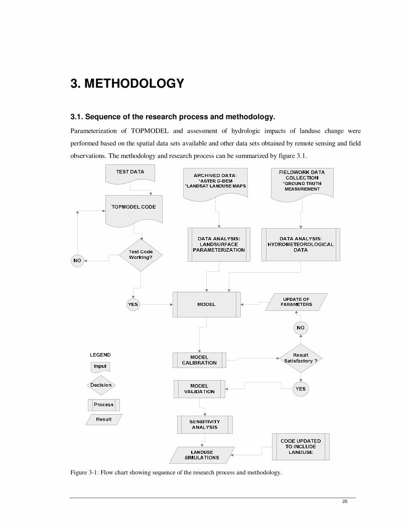
25
3. METHODOLOGY
3.1. Sequence of the research process and methodology.
Parameterization of TOPMODEL and assessment of hydrologic impacts of landuse change were
performed based on the spatial data sets available and other data sets obtained by remote sensing and field
observations. The methodology and research process can be summarized by figure 3.1.
Figure 3-1: Flow chart showing sequence of the research process and methodology.
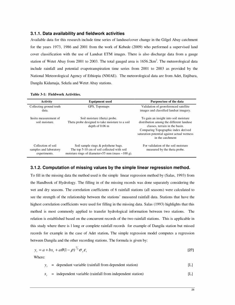
26
3.1.1. Data availability and fieldwork activities
Available data for this research include time series of landuse/cover change in the Gilgel Abay catchment
for the years 1973, 1986 and 2001 from the work of Kebede (2009) who performed a supervised land
cover classification with the use of Landsat ETM images. There is also discharge data from a gauge
station of Wetet Abay from 2001 to 2003. The total gauged area is 1656.2km2. The meteorological data
include rainfall and potential evapotranspiration time series from 2001 to 2003 as provided by the
National Meteorological Agency of Ethiopia (NMAE). The meteorological data are from Adet, Enjibara,
Dangila Kidamaja, Sekela and Wetet Abay stations.
Table 3-1: Fieldwork Activities.
Activity Equipment used Purpose/use of the data
Collecting ground truth
data.
GPS, Topomaps Validation of georeferenced satellite
images and classified landsat imagery.
Insitu measurement of
soil moisture.
Soil moisture (theta) probe.
Theta probe designed to take moisture to a soil
depth of 0.06 m
To gain an insight into soil moisture
distribution among the different landuse
classes, terrain in the basin.
Comparing Topographic index derived
saturation potential against actual wetness
in the catchment
Collection of soil
samples and laboratory
experiments.
Soil sample rings & polythene bags.
The top 5-10 cm of soil collected with soil
moisture rings of diameter=55 mm (mass ~100 g).
For validation of the soil moisture
measured by the theta probe.
3.1.2. Computation of missing values by the simple linear regression method.
To fill in the missing data the method used is the simple linear regression method by (Salas, 1993) from
the Handbook of Hydrology. The filling in of the missing records was done separately considering the
wet and dry seasons. The correlation coefficients of 6 rainfall stations (all seasons) were calculated to
see the strength of the relationship between the stations’ measured rainfall data. Stations that have the
highest correlation coefficients were used for filling in the missing data. Salas (1993) highlights that this
method is most commonly applied to transfer hydrological information between two stations. The
relation is established based on the concurrent records of the two rainfall stations. This is applicable in
this study where there is l long or complete rainfall records for example of Dangila station but missed
records for example in the case of Adet station. The simple regression model computes a regression
between Dangila and the other recording stations. The formula is given by:
tytt abxay εσρθ 21
)1( −++= [27]
Where:
ty = dependant variable (rainfall from dependent station) [L]
tx = independent variable (rainfall from independent station) [L]
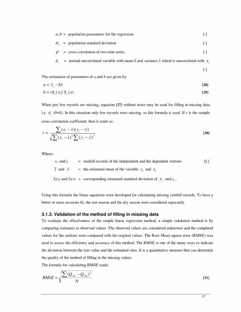
27
ba, = population parameters for the regression [-]
yσ = population standard deviation [-]
ρ = cross correlation of two time series [-]
tε = normal uncorrelated variable with mean 0 and variance 1 which is uncorrelated with tx
[-]
The estimation of parameters of a and b are given by
xbya t −= [28]
)()( 11 xSyrSb = [29]
When just few records are missing, equation [27] without noise may be used for filling in missing data
i.e. tε (θ=0). In this situation only few records were missing, so this formula is used. If r is the sample
cross correlation coefficient, then it reads as:
∑ ∑∑
−−
−−=
22 )()(
))((
yyxx
yyxxr
ii
ii [30]
Where:
xi and yi = rainfall records of the independent and the dependent stations [L]
y and x = the estimated mean of the variable ty and tx
Si(y) and Si(x) = corresponding estimated standard deviation of ty and tx ,
Using this formula the linear equations were developed for calculating missing rainfall records. To have a
better or more accurate fit, the wet season and the dry season were considered separately.
3.1.3. Validation of the method of filling in missing data
To evaluate the effectiveness of the simple linear regression method, a simple validation method is by
comparing estimates to observed values. The observed values are considered unknowns and the completed
values for the stations were compared with the original values. The Root Mean square error (RMSE) was
used to assess the efficiency and accuracy of this method. The RMSE is one of the many ways to indicate
the deviation between the true value and the estimated ones. It is a quantitative measure that can determine
the quality of the method of filling in the missing values.
The formula for calculating RMSE reads:
N
QQRMSE
simobs∑ −=
2)( [31]
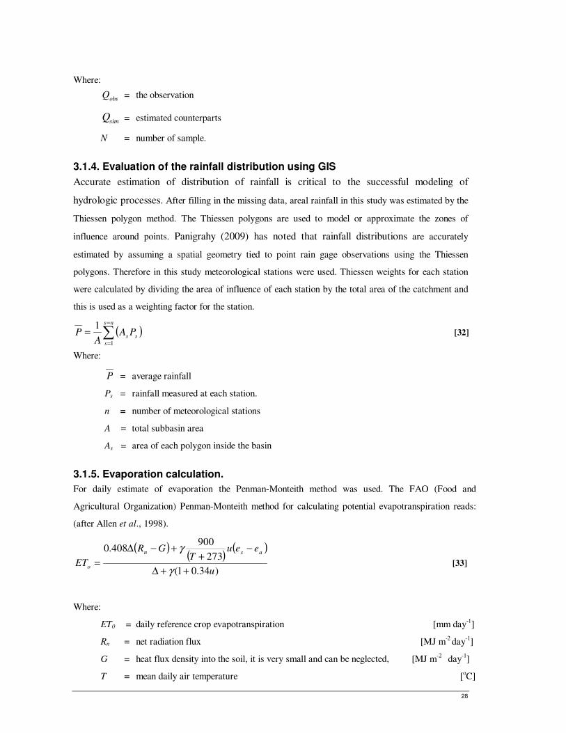
28
Where:
obsQ = the observation
simQ = estimated counterparts
N = number of sample.
3.1.4. Evaluation of the rainfall distribution using GIS
Accurate estimation of distribution of rainfall is critical to the successful modeling of
hydrologic processes. After filling in the missing data, areal rainfall in this study was estimated by the
Thiessen polygon method. The Thiessen polygons are used to model or approximate the zones of
influence around points. Panigrahy (2009) has noted that rainfall distributions are accurately
estimated by assuming a spatial geometry tied to point rain gage observations using the Thiessen
polygons. Therefore in this study meteorological stations were used. Thiessen weights for each station
were calculated by dividing the area of influence of each station by the total area of the catchment and
this is used as a weighting factor for the station.
( )∑=
=
=ns
s
ss PAA
P1
1 [32]
Where:
P = average rainfall
Ps = rainfall measured at each station.
n = number of meteorological stations
A = total subbasin area
As = area of each polygon inside the basin
3.1.5. Evaporation calculation.
For daily estimate of evaporation the Penman-Monteith method was used. The FAO (Food and
Agricultural Organization) Penman-Monteith method for calculating potential evapotranspiration reads:
(after Allen et al., 1998).
( )( )
( )
)34.01(
273
900408.0
u
eeuT
GR
ET
asn
o++∆
−+
+−∆
=γ
γ
[33]
Where:
ET0 = daily reference crop evapotranspiration [mm day-1
]
Rn = net radiation flux [MJ m-2
day-1
]
G = heat flux density into the soil, it is very small and can be neglected, [MJ m-2
day-1
]
T = mean daily air temperature [oC]
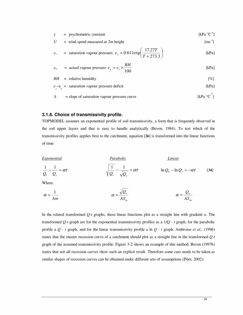
29
γ = psychometric constant [kPa oC
-1]
U = wind speed measured at 2m height [ms-1
]
es = saturation vapour pressure,
+=
3.273
27.17exp611.0
T
Tes [kPa]
ea = actual vapour pressure 100
RHee sa ×= [kPa]
RH = relative humidity [%]
es−e
a = saturation vapour pressure deficit [kPa]
∆ = slope of saturation vapour pressure curve [kPa °C-1
]
3.1.6. Choice of transmissivity profile.
TOPMODEL assumes an exponential profile of soil transmissivity, a form that is frequently observed in
the soil upper layers and that is easy to handle analytically (Beven, 1984). To test which of the
transmissivity profiles applies best to the catchment, equation [26] is transformed into the linear functions
of time:
Exponential Parabolic Linear
ατ=−st QQ
11 ατ=−
sr QQ
11 ατ−=− sb QQ lnln [34]
Where:
Am
1=α
m
o
AS
Q=α
m
o
AS
Q=α
In the related transformed Q-t graphs, these linear functions plot as a straight line with gradient α. The
transformed Q-t graph are for the exponential transmissivity profiles as a 1/Q - t graph, for the parabolic
profile a Q - t graph, and for the linear transmissivity profile a ln Q - t graph. Ambroise et al., (1996)
states that the master recession curve of a catchment should plot as a straight line in the transformed Q-t
graph of the assumed transmissivity profile. Figure 3-2 shows an example of this method. Beven (1997b)
states that not all recession curves show such an explicit result. Therefore some care needs to be taken as
similar shapes of recession curves can be obtained under different sets of assumptions (Pilot, 2002).
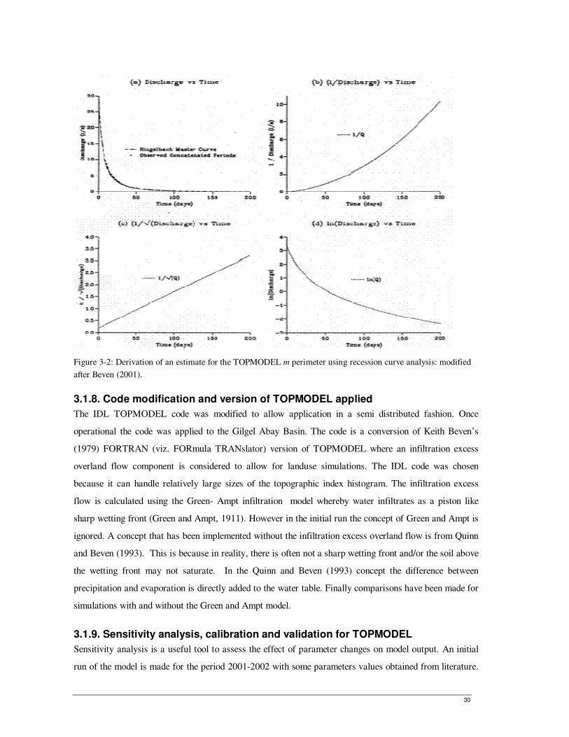
30
Figure 3-2: Derivation of an estimate for the TOPMODEL m perimeter using recession curve analysis: modified
after Beven (2001).
3.1.8. Code modification and version of TOPMODEL applied
The IDL TOPMODEL code was modified to allow application in a semi distributed fashion. Once
operational the code was applied to the Gilgel Abay Basin. The code is a conversion of Keith Beven’s
(1979) FORTRAN (viz. FORmula TRANslator) version of TOPMODEL where an infiltration excess
overland flow component is considered to allow for landuse simulations. The IDL code was chosen
because it can handle relatively large sizes of the topographic index histogram. The infiltration excess
flow is calculated using the Green- Ampt infiltration model whereby water infiltrates as a piston like
sharp wetting front (Green and Ampt, 1911). However in the initial run the concept of Green and Ampt is
ignored. A concept that has been implemented without the infiltration excess overland flow is from Quinn
and Beven (1993). This is because in reality, there is often not a sharp wetting front and/or the soil above
the wetting front may not saturate. In the Quinn and Beven (1993) concept the difference between
precipitation and evaporation is directly added to the water table. Finally comparisons have been made for
simulations with and without the Green and Ampt model.
3.1.9. Sensitivity analysis, calibration and validation for TOPMODEL
Sensitivity analysis is a useful tool to assess the effect of parameter changes on model output. An initial
run of the model is made for the period 2001-2002 with some parameters values obtained from literature.
31
Values for each chosen parameter is varied across the range provided from literature as described by
Beven and Kirkby (1979) while keeping the values of the other parameters fixed. Having gained a
knowledge of which parameters are most sensitive, 3 parameters were chosen to further evaluate model
sensitivity. These are the soil hydraulic conductivity decay parameter (m), the soil transmissivity at
saturation (To) and the root zone available water capacity (SRmax).
Calibration for the period 2001-2002 was done manually by ‘trial and error’ where the TOPMODEL
parameters are manually changed to optimize model performance. For each model run, parameter values
in the text file containing parameters are changed. Calibration was to optimize the model efficiency by
first fitting the baseflow recession. After calibration of the baseflow the peak flows were fitted. For
example m, SRmax, and TO parameters were adjusted until the recession tail matched, then the peak flow
and finally the runoff volume of the simulated hydrograph best matched the observed hydrograph. These
parameters were also adjusted until the rising limb of the simulated hydrograph and timing of the peak
flow closely matched the observed hydrograph. By optimizing the SRmax parameter, the timing of the peak
flow could be improved since a higher value of SRmax results in a model response that cause better fit of
rising limb.
Model validation has been carried out to test whether the model, using the same parameter set obtained by
optimisation (2001-2002 period), but with independent data sets, can produce outputs with reasonable
accuracy. The model has been validated using the 2003 data set. The parameters found by calibration
were used for validation of the model. The parameter values were initially set based on expected ranges
and also based on best fits of outputs. As such the simulated streamflow is compared to observed
streamflow. This is done graphically (visual comparison) or numerically (comparison of observed and
predicted values) using performance measures. The performance measures used in this study are the
Nash-Sutcliffe Efficiency (NS) and Relative Volume Error (RVE).
Nash-Sutcliffe efficiency
The Nash-Sutcliffe efficiency measure goes to 1 as the fit improves. A value between 0.6 and 0.8
indicates that the model performs reasonably. Values between 0.8 and 0.9 indicate that the model
performs very well and values between 0.90 and 1.0 indicate that the model performs extremely well
(Nash and Sutcliffe, 1970). The formula for Nash-Sutcliffe (NS) reads:
∑
∑
=
=
−
−
−=N
i
obsobs
N
i
simobs
R
1
2
1
2
2
)(
)(
1 [35]
32
Where:
obsQ = the observed discharge [L3T
-1]
simQ = predicted observed discharge [L3T
-1]
obsQ = the observed mean. [L3T
-1]
N = the total number of time steps [-]
Relative Volume Error (RVE)
The second performance measure, the RVE is used for quantifying the volume errors. This RVE can vary
between ∞ and - ∞ but performs best when a value of 0 is generated since no difference between simulated
and observed discharge occurs (Janssen and Heuberger, 1995). A relative volume error less than +5% or -
5% indicates that a model performs well while relative volume errors between +5% and +10% and -5%
and -10% indicate a model with reasonable performance.
%100*)(
−=
∑∑
obs
obssim
EQ
QQRV [36]
3.2. Parameterization of land-use in TOPMODEL.
Landuse change in any catchment affect many processes like evapotranspiration, resistance to surface
runoff, interception, and shading from solar radiation among others. A description of how these
processes are implemented in TOPMODEL is done.
3.2.1. Soil Adjusted Vegetation Index (SAVI)
SAVI is the Soil Adjusted Vegetation Index, which was introduced by Huete (1988). The initial
construction of this index was based on measurements of cotton and range grass canopies with dark and
light soil backgrounds. The SAVI reads:
( )( )LRNIR
RNIRLSAVI
++
−+=
1
[37]
Where:
NIR = near-infrared reflection
R = red reflection
L = soil adjustment factor, most often defined as 0.5.
The adjustment factor 'L' was found by trial and error until a factor that gave equal vegetation index
results for the dark and light soils was found (Huete, 1988). The standard value of L typically used in
most applications is 0.5, which is for intermediate vegetation densities. Negative SAVI indicates presence
of water.
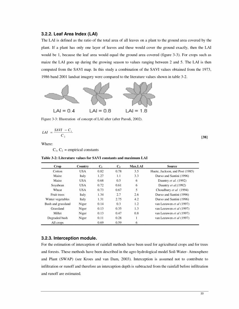
33
3.2.2. Leaf Area Index (LAI)
The LAI is defined as the ratio of the total area of all leaves on a plant to the ground area covered by the
plant. If a plant has only one layer of leaves and these would cover the ground exactly, then the LAI
would be 1, because the leaf area would equal the ground area covered (figure 3-3). For crops such as
maize the LAI goes up during the growing season to values ranging between 2 and 5. The LAI is then
computed from the SAVI map. In this study a combination of the SAVI values obtained from the 1973,
1986 band 2001 landsat imagery were compared to the literature values shown in table 3-2.
Figure 3-3: Illustration of concept of LAI after (after Parodi, 2002).
2
1
C
CSAVILAI
−=
[38]
Where:
C1, C2 = empirical constants
Table 3-2: Literature values for SAVI constants and maximum LAI
Crop Country C1 C2 Max.LAI Source
Cotton USA 0.82 0.78 3.5 Huete, Jackson, and Post (1985)
Maize Italy 1.27 1.1 3.3 Durso and Santini (1996)
Maize USA 0.68 0.5 6 Dauntry et al. (1992)
Soyabean USA 0.72 0.61 6 Dauntry et al.(1992)
Wheat USA 0.73 0.67 5 Choudhury et al (1994)
Fruit trees Italy 1.34 2.7 2.6 Durso and Santini (1996)
Winter vegetables Italy 1.31 2.75 4.2 Durso and Santini (1996)
Bush and grassland Niger 0.14 0.3 1.2 van Leeuwen et al (1997)
Grassland Niger 0.13 0.35 1.3 van Leeuwen et al (1997)
Millet Niger 0.13 0.47 0.8 van Leeuwen et al (1997)
Degraded bush Niger 0.11 0.28 1 van Leeuwen et al (1997)
All crops 0.69 0.59 6
3.2.3. Interception module.
For the estimation of interception of rainfall methods have been used for agricultural crops and for trees
and forests. These methods have been described in the agro hydrological model Soil-Water- Atmosphere
and Plant (SWAP) (see Kroes and van Dam, 2003). Interception is assumed not to contribute to
infiltration or runoff and therefore an interception depth is subtracted from the rainfall before infiltration
and runoff are estimated.
34
Agricultural crops and grasslands
The interception of precipitation can be highly variable in space and time, particularly in catchments
with mixed land use, so an interception module (figure 3-4) based on Dam (2000) was used:
+
−=
aLAI
bPaLAIP
gross
i
1
11 [39]
Where:
Pi = intercepted precipitation [cm]
LAI = leaf area index [m2 m
-2]
Pgross = gross precipitation [cm]
a = empirical coefficient [cm]
b = the soil cover fraction (=LAI/3.0) [-]
The method is an assumption that the amount of interception storage asymptotically reaches a maximum
value that is factored in the a LAI part of equation [39] (Braden, 1985). Therefore the aLAI term is
called the saturation amount. In principle a must be determined experimentally but in this work all
parameters were obtained from the literature and from landuse maps. In agricultural crops a value of a
= 0.25 was assumed following Dam (2000). This interception model has been applied in such as the
Soil-Water-Atmosphere-Plant (SWAP) model.
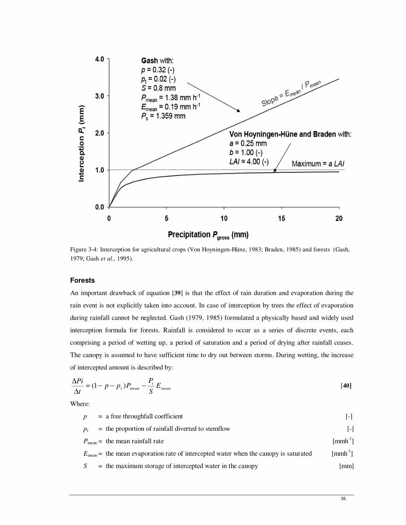
35
Figure 3-4: Interception for agricultural crops (Von Hoyningen-Hüne, 1983; Braden, 1985) and forests (Gash,
1979; Gash et al., 1995).
Forests
An important drawback of equation [39] is that the effect of rain duration and evaporation during the
rain event is not explicitly taken into account. In case of interception by trees the effect of evaporation
during rainfall cannot be neglected. Gash (1979, 1985) formulated a physically based and widely used
interception formula for forests. Rainfall is considered to occur as a series of discrete events, each
comprising a period of wetting up, a period of saturation and a period of drying after rainfall ceases.
The canopy is assumed to have sufficient time to dry out between storms. During wetting, the increase
of intercepted amount is described by:
mean
i
meant ES
PPpp
t
Pi−−−=
∆
∆)1( [40]
Where:
p = a free throughfall coefficient [-]
pt = the proportion of rainfall diverted to stemflow [-]
Pmean = the mean rainfall rate [mmh-1
]
Emean = the mean evaporation rate of intercepted water when the canopy is saturated [mmh-1]
S = the maximum storage of intercepted water in the canopy [mm]
36
Integration of equation [40] yields the amount of rainfall, Ps [mm] which saturates the canopy:
−−−=
)1(1ln
tmean
mean
mean
mean
sppP
ES
E
PP with 0
)1(1 ≥
−−−
tmean
mean
ppP
E [41]
For small storms )( sgross PP < the interception can be calculated from:
grossti PppP )1( −−= [42]
For large storms ( sgross PP > ) the interception according to Gash (1979) follows from:
)()1( sgross
mean
mean
sti PPP
EPppP −+−−= [43]
Figure 3-4 shows the relation of Gash for typical values of a pine forest as a function of rainfall
amounts. The slope
grossP
Pi
∆
∆before saturation of the canopy equals (1-p-pt), while after saturation this
slope equals Emean/Pmean. This analytical model has been used with considerable success to predict
interception in a wide range of environments including the Tai forest of Ivory Coast by Hutjes (1990).
3.2.4. Evapotranspiration calculated using the crop coefficient approach
Evapotranspiration from each specific vegetation type or crop evapotranspiration (ETc) is calculated
using the crop coefficient approach (Kc) from the FAO Irrigation and Drainage Paper No. 56 (Allen et
al., 1998). In the crop coefficient approach, crop evapotranspiration is calculated by multiplying the
reference evapotranspiration (ETo) by Kc as follows:
occ ETKET = [44]
Where:
ETc = crop evapotranspiration [mm d-1]
Kc = crop coefficient [mm d-1]
ETo = reference crop evapotranspiration [mm d-1
]
The crop evapotranspiration differs distinctly from the reference evapotranspiration as the ground
cover, canopy properties and aerodynamic resistance of the crop are different from grass. The effects of
characteristics that differentiate different vegetation types from grass are integrated into the single crop
coefficient (Kc). The Kc varies predominately with the specific crop characteristics while climatic
settings only have marginal effects. This enables the transfer of standard values for Kc between
locations and between climates. The reference ETo is defined and calculated using the FAO Penman-
Monteith as in Equation [33]. The crop coefficient, Kc is basically the ratio of the crop ETc to the
reference ETo, and it represents an integration of the effects of four primary characteristics that
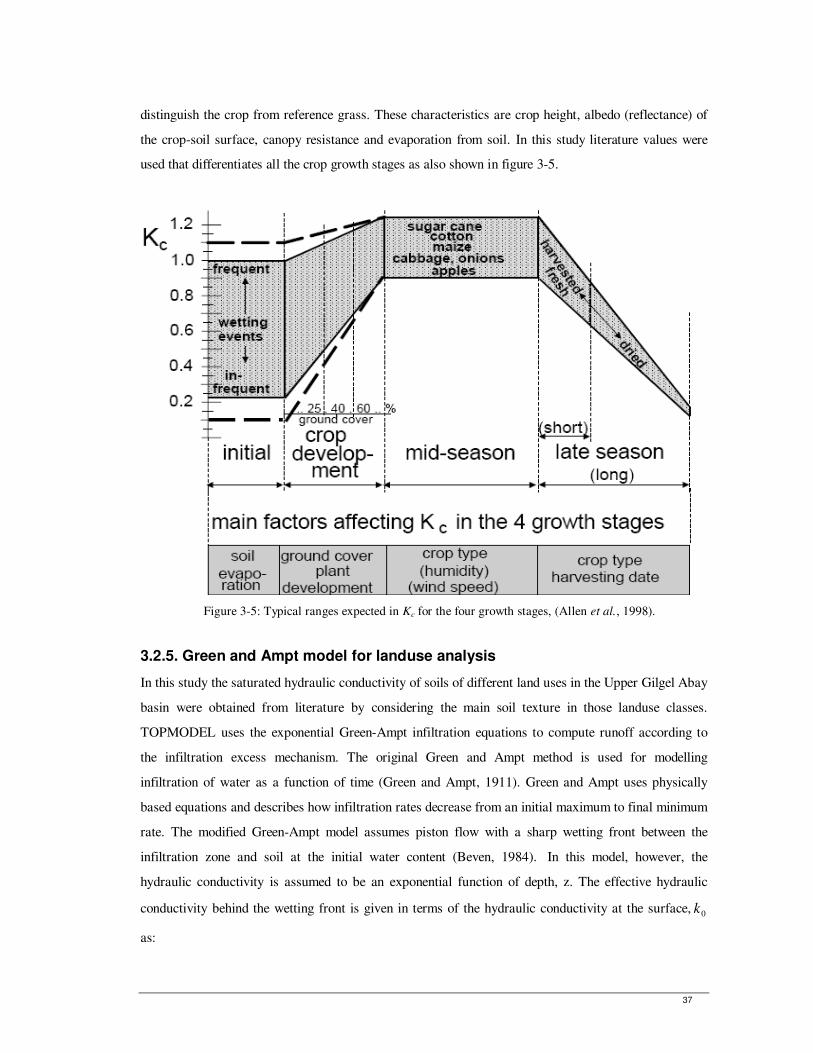
37
distinguish the crop from reference grass. These characteristics are crop height, albedo (reflectance) of
the crop-soil surface, canopy resistance and evaporation from soil. In this study literature values were
used that differentiates all the crop growth stages as also shown in figure 3-5.
Figure 3-5: Typical ranges expected in Kc for the four growth stages, (Allen et al., 1998).
3.2.5. Green and Ampt model for landuse analysis
In this study the saturated hydraulic conductivity of soils of different land uses in the Upper Gilgel Abay
basin were obtained from literature by considering the main soil texture in those landuse classes.
TOPMODEL uses the exponential Green-Ampt infiltration equations to compute runoff according to
the infiltration excess mechanism. The original Green and Ampt method is used for modelling
infiltration of water as a function of time (Green and Ampt, 1911). Green and Ampt uses physically
based equations and describes how infiltration rates decrease from an initial maximum to final minimum
rate. The modified Green-Ampt model assumes piston flow with a sharp wetting front between the
infiltration zone and soil at the initial water content (Beven, 1984). In this model, however, the
hydraulic conductivity is assumed to be an exponential function of depth, z. The effective hydraulic
conductivity behind the wetting front is given in terms of the hydraulic conductivity at the surface, 0k
as:

38
fZekzk 0)( = [45]
Where:
0k = the hydraulic conductivity at the surface [LT-1
]
z = depth below soil surface [L]
f = constant
If the wetting front has reached a depth z, the infiltration rate, i is given by the generalization of the
relationship for layered soils (Childs and Bybordi, 1969)
∫=
=
+∆==
Zz
zzkdz
z
dt
dIi
0])(/[
ψ [46]
Where I is the cumulative infiltration [L]
In the approach it is assumed that at the time of ponding pt , the wetting front is at a depth pZ which is
given by the infiltration rate pI divided by the change in moisture content θ∆
θ∆= /pp Iz [47]
The cumulative infiltration at the time of ponding is given by:
pp rtI = [48]
Where:
r = the rain rate
At the onset of ponding the rain rate r is assumed to be equal to the infiltration rate i and the infiltration
rate is given by
θ
θψ∆−−
∆+∆=
/
0
1
)/(
PfI
p
e
Ifkr [49]
At any time after ponding has started, the cumulative infiltration is I and the infiltration rate is given by:
θ
θψ∆−−
∆+∆×=
/
0
1
)/(fI
e
Ifk
dt
dI [50]
The time required for the surface to reach saturation is the time to ponding. Ponding will only occur
when the rain rate is greater than or equal to the hydraulic conductivity at the surface. The time to
ponding, tp, is calculated as:
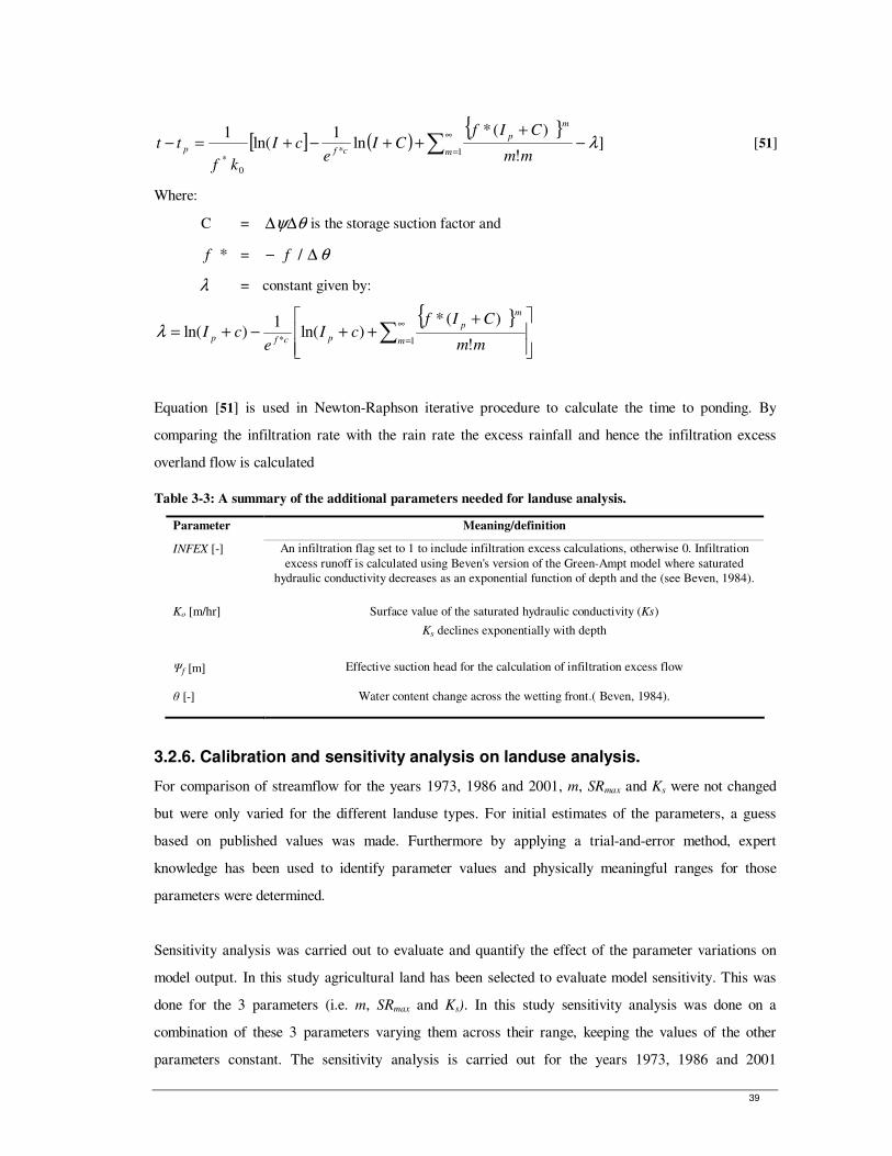
39
[ ] ( )}{
]!
)(*ln
1ln(
11*
0
*
λ−+
++−+=− ∑∞
=m
m
p
cfpmm
CIfCI
ecI
kf
tt [51]
Where:
C = θψ∆∆ is the storage suction factor and
*f = θ∆− /f
λ = constant given by:
}{
+++−+= ∑
∞
=1* !
)(*)ln(
1)ln(
m
m
p
pcfpmm
CIfcI
ecIλ
Equation [51] is used in Newton-Raphson iterative procedure to calculate the time to ponding. By
comparing the infiltration rate with the rain rate the excess rainfall and hence the infiltration excess
overland flow is calculated
Table 3-3: A summary of the additional parameters needed for landuse analysis.
Parameter Meaning/definition
INFEX [-] An infiltration flag set to 1 to include infiltration excess calculations, otherwise 0. Infiltration
excess runoff is calculated using Beven's version of the Green-Ampt model where saturated
hydraulic conductivity decreases as an exponential function of depth and the (see Beven, 1984).
Ko [m/hr] Surface value of the saturated hydraulic conductivity (Ks)
Ks declines exponentially with depth
Ψf [m] Effective suction head for the calculation of infiltration excess flow
θ [-] Water content change across the wetting front.( Beven, 1984).
3.2.6. Calibration and sensitivity analysis on landuse analysis.
For comparison of streamflow for the years 1973, 1986 and 2001, m, SRmax and Ks were not changed
but were only varied for the different landuse types. For initial estimates of the parameters, a guess
based on published values was made. Furthermore by applying a trial-and-error method, expert
knowledge has been used to identify parameter values and physically meaningful ranges for those
parameters were determined.
Sensitivity analysis was carried out to evaluate and quantify the effect of the parameter variations on
model output. In this study agricultural land has been selected to evaluate model sensitivity. This was
done for the 3 parameters (i.e. m, SRmax and Ks). In this study sensitivity analysis was done on a
combination of these 3 parameters varying them across their range, keeping the values of the other
parameters constant. The sensitivity analysis is carried out for the years 1973, 1986 and 2001
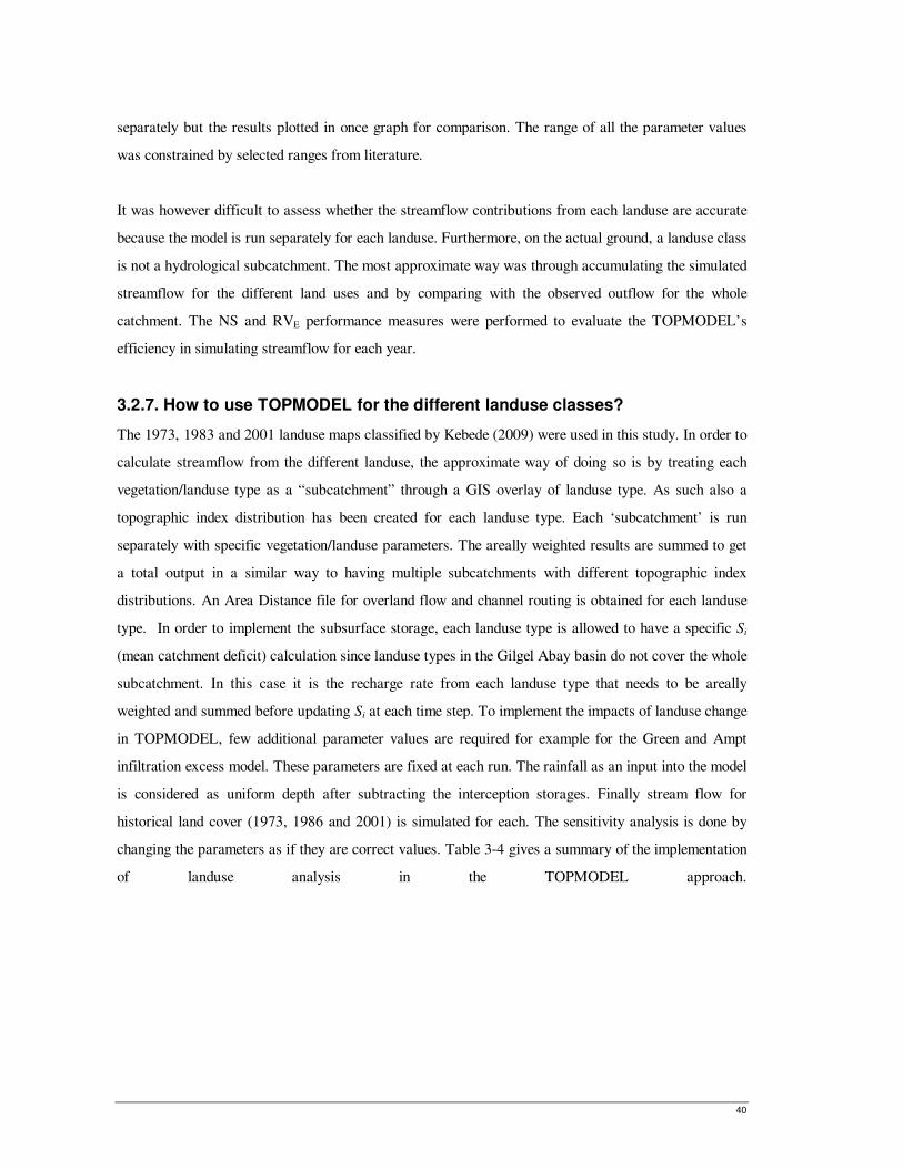
40
separately but the results plotted in once graph for comparison. The range of all the parameter values
was constrained by selected ranges from literature.
It was however difficult to assess whether the streamflow contributions from each landuse are accurate
because the model is run separately for each landuse. Furthermore, on the actual ground, a landuse class
is not a hydrological subcatchment. The most approximate way was through accumulating the simulated
streamflow for the different land uses and by comparing with the observed outflow for the whole
catchment. The NS and RVE performance measures were performed to evaluate the TOPMODEL’s
efficiency in simulating streamflow for each year.
3.2.7. How to use TOPMODEL for the different landuse classes?
The 1973, 1983 and 2001 landuse maps classified by Kebede (2009) were used in this study. In order to
calculate streamflow from the different landuse, the approximate way of doing so is by treating each
vegetation/landuse type as a “subcatchment” through a GIS overlay of landuse type. As such also a
topographic index distribution has been created for each landuse type. Each ‘subcatchment’ is run
separately with specific vegetation/landuse parameters. The areally weighted results are summed to get
a total output in a similar way to having multiple subcatchments with different topographic index
distributions. An Area Distance file for overland flow and channel routing is obtained for each landuse
type. In order to implement the subsurface storage, each landuse type is allowed to have a specific Si
(mean catchment deficit) calculation since landuse types in the Gilgel Abay basin do not cover the whole
subcatchment. In this case it is the recharge rate from each landuse type that needs to be areally
weighted and summed before updating Si at each time step. To implement the impacts of landuse change
in TOPMODEL, few additional parameter values are required for example for the Green and Ampt
infiltration excess model. These parameters are fixed at each run. The rainfall as an input into the model
is considered as uniform depth after subtracting the interception storages. Finally stream flow for
historical land cover (1973, 1986 and 2001) is simulated for each. The sensitivity analysis is done by
changing the parameters as if they are correct values. Table 3-4 gives a summary of the implementation
of landuse analysis in the TOPMODEL approach.
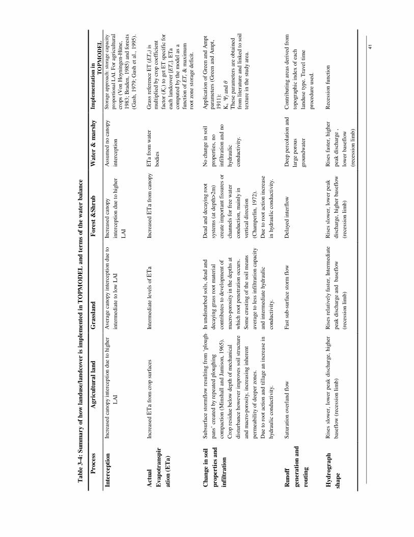
41
Ta
ble
3-4
: S
um
ma
ry
of
how
lan
du
se/l
an
dco
ver i
s im
ple
men
ted
in
TO
PM
OD
EL
an
d t
erm
s of
the w
ate
r b
ala
nce
Process
A
gric
ult
ura
l la
nd
G
rass
lan
d
Fore
st &
Sh
ru
b
Wa
ter &
ma
rsh
y
Imp
lem
enta
tion
in
TO
PM
OD
EL
Inte
rcep
tion
In
crea
sed
can
op
y in
terc
epti
on d
ue
to h
igher
LA
I
Aver
age
canop
y in
terc
epti
on
du
e to
inte
rmed
iate
to l
ow L
AI
Incr
ease
d c
anop
y
inte
rcep
tion
du
e to
hig
her
LA
I
Ass
um
ed n
o c
anop
y
inte
rcep
tion
Sto
rage
ap
pro
ach
: st
ora
ge c
ap
aci
ty
pro
port
ional L
AI.
For
agri
cult
ura
l
crops
(Von
Hoyn
ingen
-Hü
ne,
19
83
; B
rad
en,
19
85
) an
d f
ore
sts
(Gas
h,
197
9;
Gas
h e
t al
., 1
995
).
Actu
al
Evap
otr
an
spir
ati
on
(E
Ta
)
Incr
ease
d E
Ta
fro
m c
rop s
urf
aces
In
term
edia
te l
evel
s of
ET
a
Incr
ease
d E
Ta
from
can
op
y E
Ta
from
wat
er
bodie
s
Gra
ss r
efer
ence
ET
(E
To)
is
mult
ipli
ed b
y cr
op
coef
fici
ent
fact
or
(Kc)
to g
et E
T s
pec
ific
for
each
lan
dco
ver
[E
Tc]
. E
Ta
com
pu
ted b
y th
e m
od
el a
s a
fun
ctio
n o
f E
Tc &
max
imu
m
root
zon
e st
ora
ge
def
icit
.
Ch
an
ge i
n s
oil
prop
erti
es a
nd
infi
ltra
tion
Su
bsu
rfac
e st
orm
flow
res
ult
ing f
rom
‘plo
ugh
-
pan
s’ c
reat
ed b
y re
pea
ted
plo
ugh
ing
com
pac
tion
(M
insh
all
and
Jam
ison,
19
65
).
Cro
p r
esid
ue
bel
ow
dep
th o
f m
ech
anic
al
dis
turb
ance
how
ever
im
pro
ves
soil
str
uct
ure
and
mac
ro-p
oro
sity
, in
crea
sing i
nh
eren
t
per
mea
bil
ity
of
dee
per
zon
es.
Du
e to
root
acti
on
an
d t
illa
ge
an i
ncr
ease
in
hyd
rau
lic
con
du
ctiv
ity.
In u
nd
istu
rbed
soil
s, d
ead
an
d
dec
ayin
g g
rass
root
mat
eria
l
contr
ibu
tes
to d
evel
opm
ent
of
mac
ro-p
oro
sity
in
th
e dep
ths
at
wh
ich
root
pen
etra
tion
occ
urs
.
Som
e cr
ust
ing o
f th
e so
il m
eans
aver
age
to l
ess
infi
ltra
tion
cap
acit
y
and
in
term
edia
te h
ydra
uli
c
cond
uct
ivit
y.
Dea
d a
nd
dec
ayin
g r
oot
syst
ems
(at
dep
th>
2m
)
crea
te i
mp
ort
ant
fiss
ure
s or
chan
nel
s fo
r fr
ee w
ater
con
duct
ion
, m
ain
ly i
n
ver
tica
l d
irec
tion
(Cham
per
lin
, 1
97
2).
Du
e to
root
acti
on i
ncr
ease
in h
ydra
uli
c co
nd
uct
ivit
y.
No c
han
ge
in s
oil
pro
per
ties
, n
o
infi
ltra
tion
an
d n
o
hyd
rau
lic
con
duct
ivit
y.
Ap
pli
cati
on
of
Gre
en a
nd
Am
pt
par
amet
ers
(Gre
en a
nd A
mp
t,
19
11
):
Ks
Ψf an
d θ
Th
ese
par
amet
ers
are
ob
tain
ed
from
lit
erat
ure
an
d l
ink
ed t
o so
il
tex
ture
in
th
e st
ud
y ar
ea.
Ru
noff
gen
era
tion
an
d
rou
tin
g
Sat
ura
tion
over
lan
d f
low
F
ast
sub
-su
rfac
e st
orm
flo
w
Del
ayed
in
terf
low
Dee
p p
erco
lati
on
and
larg
e p
oro
us
gro
un
dw
ater
Con
trib
uti
ng a
reas
der
ived
fro
m
topogra
ph
ic i
nd
ex o
f ea
ch
lan
du
se t
ype.
Tra
vel
tim
e
pro
ced
ure
use
d.
Hyd
rogra
ph
shap
e
Ris
es s
low
er,
low
er p
eak
dis
char
ge,
hig
her
bas
eflo
w (
rece
ssio
n l
imb
)
Ris
es r
elat
ivel
y fa
ster
, In
term
edia
te
pea
k d
isch
arge
and
b
asef
low
(rec
essi
on l
imb
)
Ris
es s
low
er,
low
er p
eak
dis
char
ge,
hig
her
bas
eflo
w
(rec
essi
on
lim
b)
Ris
es f
aste
r, h
igh
er
pea
k d
isch
arge
,
low
er b
asef
low
(rec
essi
on
lim
b)
Rec
essi
on
fu
nct
ion
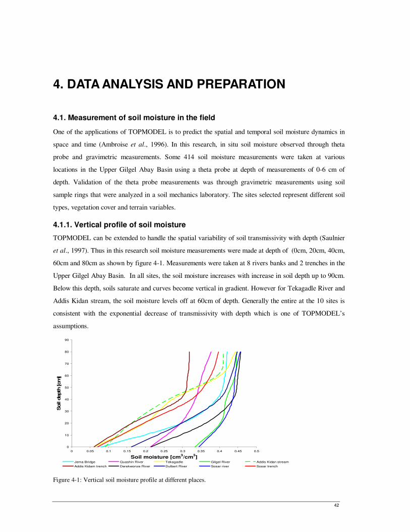
42
4. DATA ANALYSIS AND PREPARATION
4.1. Measurement of soil moisture in the field
One of the applications of TOPMODEL is to predict the spatial and temporal soil moisture dynamics in
space and time (Ambroise et al., 1996). In this research, in situ soil moisture observed through theta
probe and gravimetric measurements. Some 414 soil moisture measurements were taken at various
locations in the Upper Gilgel Abay Basin using a theta probe at depth of measurements of 0-6 cm of
depth. Validation of the theta probe measurements was through gravimetric measurements using soil
sample rings that were analyzed in a soil mechanics laboratory. The sites selected represent different soil
types, vegetation cover and terrain variables.
4.1.1. Vertical profile of soil moisture
TOPMODEL can be extended to handle the spatial variability of soil transmissivity with depth (Saulnier
et al., 1997). Thus in this research soil moisture measurements were made at depth of (0cm, 20cm, 40cm,
60cm and 80cm as shown by figure 4-1. Measurements were taken at 8 rivers banks and 2 trenches in the
Upper Gilgel Abay Basin. In all sites, the soil moisture increases with increase in soil depth up to 90cm.
Below this depth, soils saturate and curves become vertical in gradient. However for Tekagadle River and
Addis Kidan stream, the soil moisture levels off at 60cm of depth. Generally the entire at the 10 sites is
consistent with the exponential decrease of transmissivity with depth which is one of TOPMODEL’s
assumptions.
0
10
20
30
40
50
60
70
80
90
0 0.05 0.1 0.15 0.2 0.25 0.3 0.35 0.4 0.45 0.5
Soil moisture [cm3/cm
3]
Soil d
epth
[cm
]
Jema Bridge Quashin River Tekagadle Gilgel River Addis Kidan stream
Addis Kidam trench Derekwonze River Dulbert River Sosar river Sosar trench
Figure 4-1: Vertical soil moisture profile at different places.
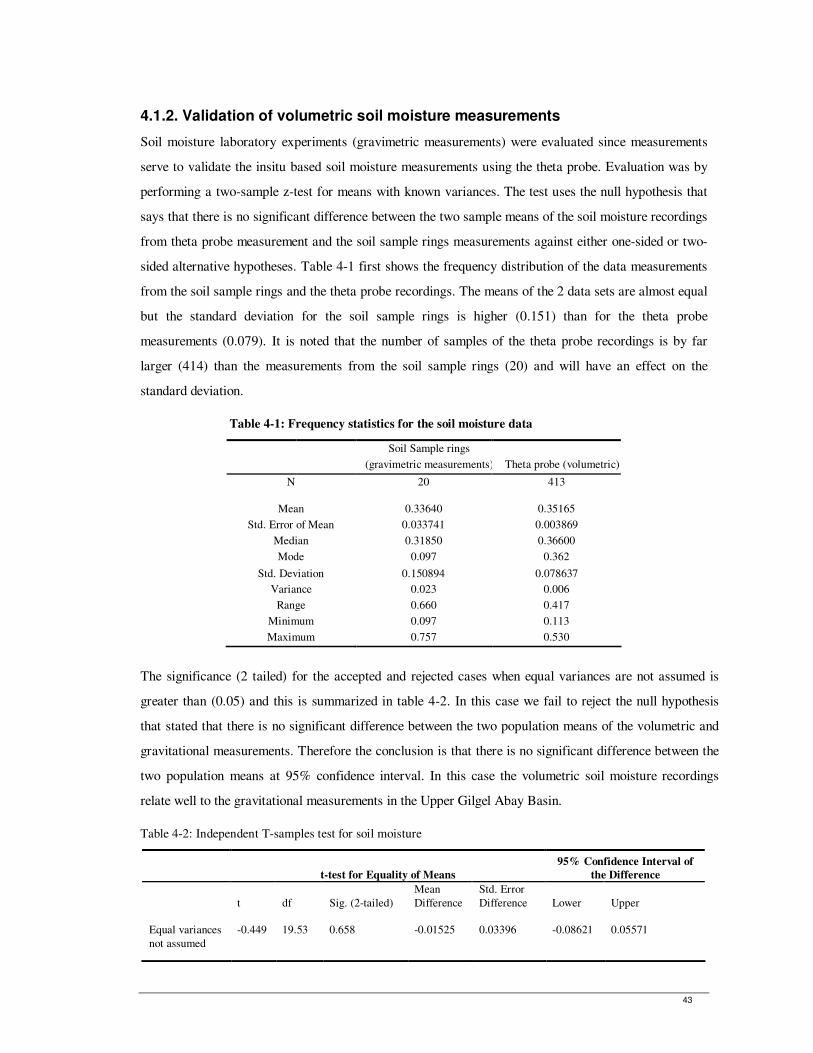
43
4.1.2. Validation of volumetric soil moisture measurements
Soil moisture laboratory experiments (gravimetric measurements) were evaluated since measurements
serve to validate the insitu based soil moisture measurements using the theta probe. Evaluation was by
performing a two-sample z-test for means with known variances. The test uses the null hypothesis that
says that there is no significant difference between the two sample means of the soil moisture recordings
from theta probe measurement and the soil sample rings measurements against either one-sided or two-
sided alternative hypotheses. Table 4-1 first shows the frequency distribution of the data measurements
from the soil sample rings and the theta probe recordings. The means of the 2 data sets are almost equal
but the standard deviation for the soil sample rings is higher (0.151) than for the theta probe
measurements (0.079). It is noted that the number of samples of the theta probe recordings is by far
larger (414) than the measurements from the soil sample rings (20) and will have an effect on the
standard deviation.
Table 4-1: Frequency statistics for the soil moisture data
Soil Sample rings
(gravimetric measurements) Theta probe (volumetric)
N
20 413
Mean 0.33640 0.35165
Std. Error of Mean 0.033741 0.003869
Median 0.31850 0.36600
Mode 0.097 0.362
Std. Deviation 0.150894 0.078637
Variance 0.023 0.006
Range 0.660 0.417
Minimum 0.097 0.113
Maximum 0.757 0.530
The significance (2 tailed) for the accepted and rejected cases when equal variances are not assumed is
greater than (0.05) and this is summarized in table 4-2. In this case we fail to reject the null hypothesis
that stated that there is no significant difference between the two population means of the volumetric and
gravitational measurements. Therefore the conclusion is that there is no significant difference between the
two population means at 95% confidence interval. In this case the volumetric soil moisture recordings
relate well to the gravitational measurements in the Upper Gilgel Abay Basin.
Table 4-2: Independent T-samples test for soil moisture
t-test for Equality of Means
95% Confidence Interval of
the Difference
t
df
Sig. (2-tailed)
Mean
Difference
Std. Error
Difference
Lower
Upper
Equal variances
not assumed
-0.449 19.53 0.658 -0.01525 0.03396 -0.08621 0.05571
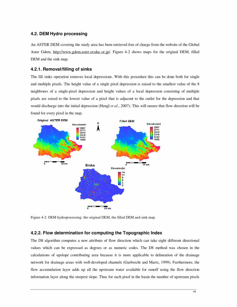
44
4.2. DEM Hydro processing
An ASTER DEM covering the study area has been retrieved free of charge from the website of the Global
Aster Gdem, http://www.gdem.aster.ersdac.or.jp/. Figure 4-2 shows maps for the original DEM, filled
DEM and the sink map.
4.2.1. Removal/filling of sinks
The fill sinks operation removes local depressions. With this procedure this can be done both for single
and multiple pixels. The height value of a single pixel depression is raised to the smallest value of the 8
neighbours of a single-pixel depression and height values of a local depression consisting of multiple
pixels are raised to the lowest value of a pixel that is adjacent to the outlet for the depression and that
would discharge into the initial depression (Hengl et al., 2007). This will ensure that flow direction will be
found for every pixel in the map.
Figure 4-2: DEM hydroprocessing: the original DEM, the filled DEM and sink map.
4.2.2. Flow determination for computing the Topographic Index
The D8 algorithm computes a new attribute of flow direction which can take eight different directional
values which can be expressed as degrees or as numeric codes. The D8 method was chosen in the
calculations of upslope contributing area because it is more applicable to delineation of the drainage
network for drainage areas with well-developed channels (Garbrecht and Martz, 1999). Furthermore, the
flow accumulation layer adds up all the upstream water available for runoff using the flow direction
information layer along the steepest slope. Thus for each pixel in the basin the number of upstream pixels
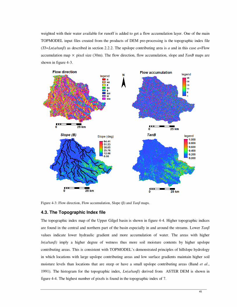
45
weighted with their water available for runoff is added to get a flow accumulation layer. One of the main
TOPMODEL input files created from the products of DEM pre-processing is the topographic index file
(TI=Ln(a/tanβ) as described in section 2.2.2. The upslope contributing area is a and in this case a=Flow
accumulation map × pixel size (30m). The flow direction, flow accumulation, slope and TanB maps are
shown in figure 4-3.
Figure 4-3: Flow direction, Flow accumulation, Slope (β) and Tanβ maps.
4.3. The Topographic Index file
The topographic index map of the Upper Gilgel basin is shown in figure 4-4. Higher topographic indices
are found in the central and northern part of the basin especially in and around the streams. Lower Tanβ
values indicate lower hydraulic gradient and more accumulation of water. The areas with higher
ln(a/tanβ) imply a higher degree of wetness thus more soil moisture contents by higher upslope
contributing areas. This is consistent with TOPMODEL’s demonstrated principles of hillslope hydrology
in which locations with large upslope contributing areas and low surface gradients maintain higher soil
moisture levels than locations that are steep or have a small upslope contributing areas (Band et al.,
1991). The histogram for the topographic index, Ln(a/tanβ) derived from ASTER DEM is shown in
figure 4-4. The highest number of pixels is found in the topographic index of 7.
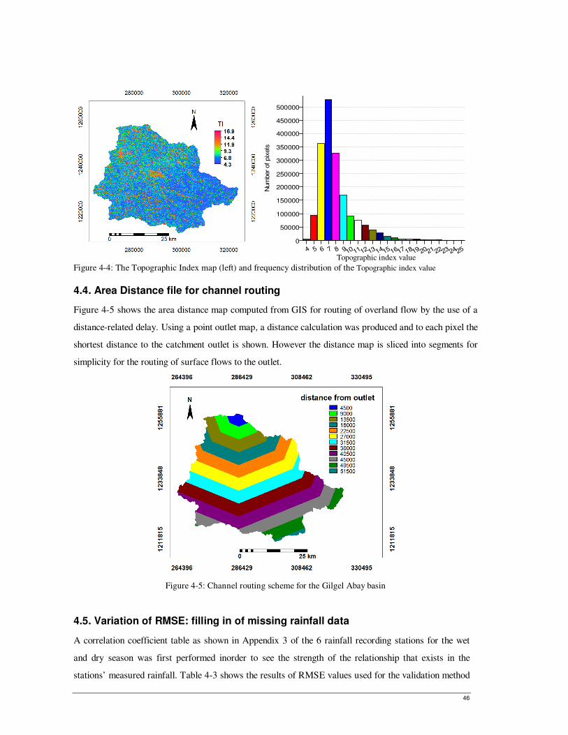
46
4 5 6 7 8 910 1112 13 1415 1617 1819 2021 2223 2425
0
50000
100000
150000
200000
250000
300000
350000
400000
450000
500000
Num
ber of pix
els
Figure 4-4: The Topographic Index map (left) and frequency distribution of the Topographic index value
4.4. Area Distance file for channel routing
Figure 4-5 shows the area distance map computed from GIS for routing of overland flow by the use of a
distance-related delay. Using a point outlet map, a distance calculation was produced and to each pixel the
shortest distance to the catchment outlet is shown. However the distance map is sliced into segments for
simplicity for the routing of surface flows to the outlet.
Figure 4-5: Channel routing scheme for the Gilgel Abay basin
4.5. Variation of RMSE: filling in of missing rainfall data
A correlation coefficient table as shown in Appendix 3 of the 6 rainfall recording stations for the wet
and dry season was first performed inorder to see the strength of the relationship that exists in the
stations’ measured rainfall. Table 4-3 shows the results of RMSE values used for the validation method
Topographic index value
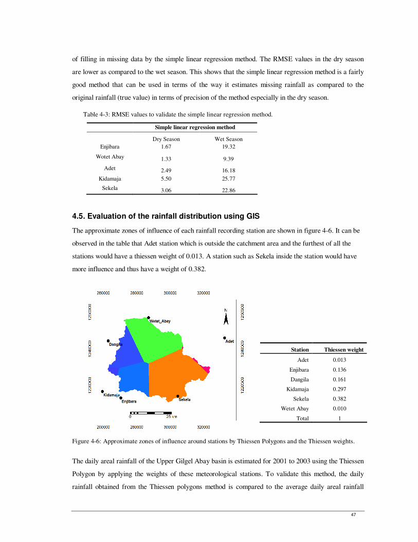
47
of filling in missing data by the simple linear regression method. The RMSE values in the dry season
are lower as compared to the wet season. This shows that the simple linear regression method is a fairly
good method that can be used in terms of the way it estimates missing rainfall as compared to the
original rainfall (true value) in terms of precision of the method especially in the dry season.
Table 4-3: RMSE values to validate the simple linear regression method.
Simple linear regression method
Dry Season Wet Season
Enjibara 1.67 19.32
Wotet Abay 1.33 9.39
Adet 2.49 16.18
Kidamaja 5.50 25.77
Sekela 3.06 22.86
4.5. Evaluation of the rainfall distribution using GIS
The approximate zones of influence of each rainfall recording station are shown in figure 4-6. It can be
observed in the table that Adet station which is outside the catchment area and the furthest of all the
stations would have a thiessen weight of 0.013. A station such as Sekela inside the station would have
more influence and thus have a weight of 0.382.
Figure 4-6: Approximate zones of influence around stations by Thiessen Polygons and the Thiessen weights.
The daily areal rainfall of the Upper Gilgel Abay basin is estimated for 2001 to 2003 using the Thiessen
Polygon by applying the weights of these meteorological stations. To validate this method, the daily
rainfall obtained from the Thiessen polygons method is compared to the average daily areal rainfall
Station Thiessen weight
Adet 0.013
Enjibara 0.136
Dangila 0.161
Kidamaja 0.297
Sekela 0.382
Wetet Abay 0.010
Total 1
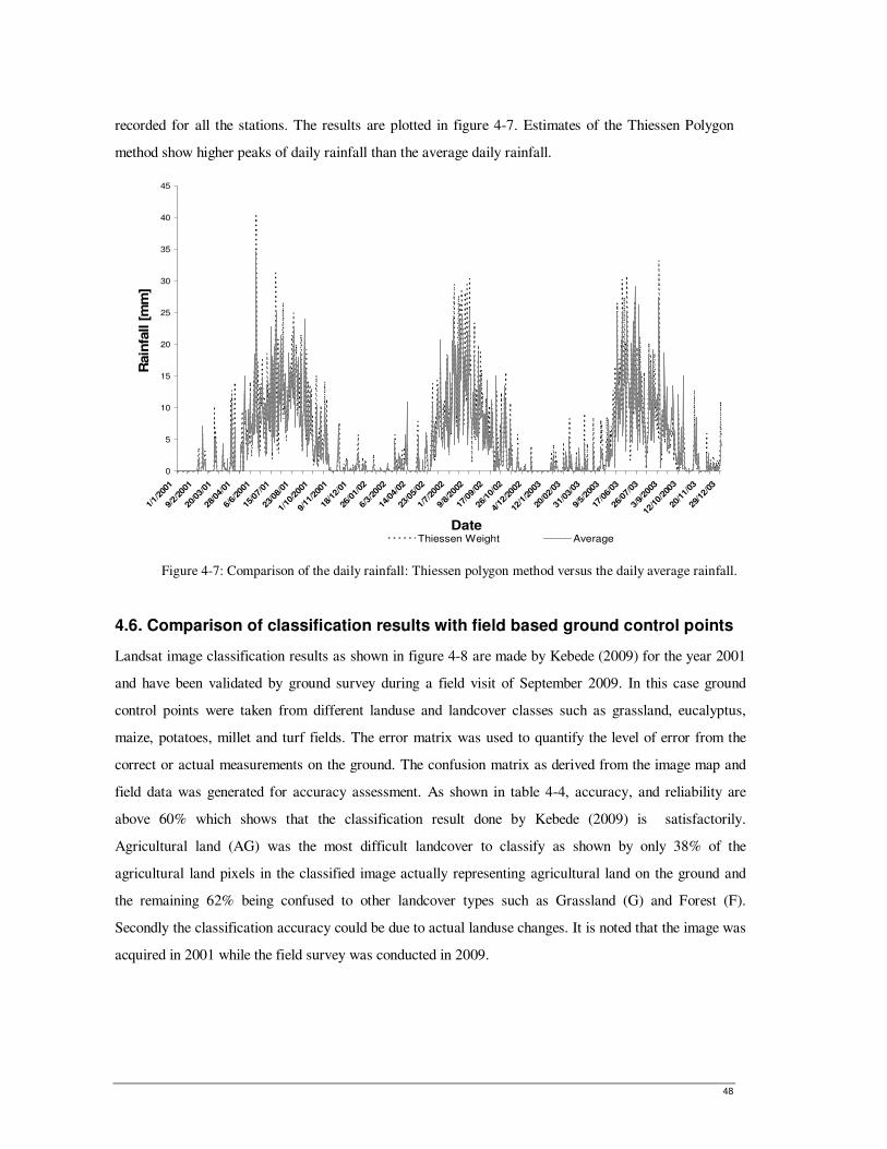
48
recorded for all the stations. The results are plotted in figure 4-7. Estimates of the Thiessen Polygon
method show higher peaks of daily rainfall than the average daily rainfall.
0
5
10
15
20
25
30
35
40
45
1/1/
2001
9/2/
2001
20/03/
01
28/0
4/01
6/6/
2001
15/07/
01
23/0
8/01
1/10
/200
1
9/11
/200
1
18/1
2/01
26/0
1/02
6/3/
2002
14/04/
02
23/0
5/02
1/7/
2002
9/8/20
02
17/0
9/02
26/10/
02
4/12
/200
2
12/1
/200
3
20/0
2/03
31/0
3/03
9/5/
2003
17/0
6/03
26/07/
03
3/9/20
03
12/10/
2003
20/11/
03
29/1
2/03
Date
Rain
fall [m
m]
Thiessen Weight Average
Figure 4-7: Comparison of the daily rainfall: Thiessen polygon method versus the daily average rainfall.
4.6. Comparison of classification results with field based ground control points
Landsat image classification results as shown in figure 4-8 are made by Kebede (2009) for the year 2001
and have been validated by ground survey during a field visit of September 2009. In this case ground
control points were taken from different landuse and landcover classes such as grassland, eucalyptus,
maize, potatoes, millet and turf fields. The error matrix was used to quantify the level of error from the
correct or actual measurements on the ground. The confusion matrix as derived from the image map and
field data was generated for accuracy assessment. As shown in table 4-4, accuracy, and reliability are
above 60% which shows that the classification result done by Kebede (2009) is satisfactorily.
Agricultural land (AG) was the most difficult landcover to classify as shown by only 38% of the
agricultural land pixels in the classified image actually representing agricultural land on the ground and
the remaining 62% being confused to other landcover types such as Grassland (G) and Forest (F).
Secondly the classification accuracy could be due to actual landuse changes. It is noted that the image was
acquired in 2001 while the field survey was conducted in 2009.
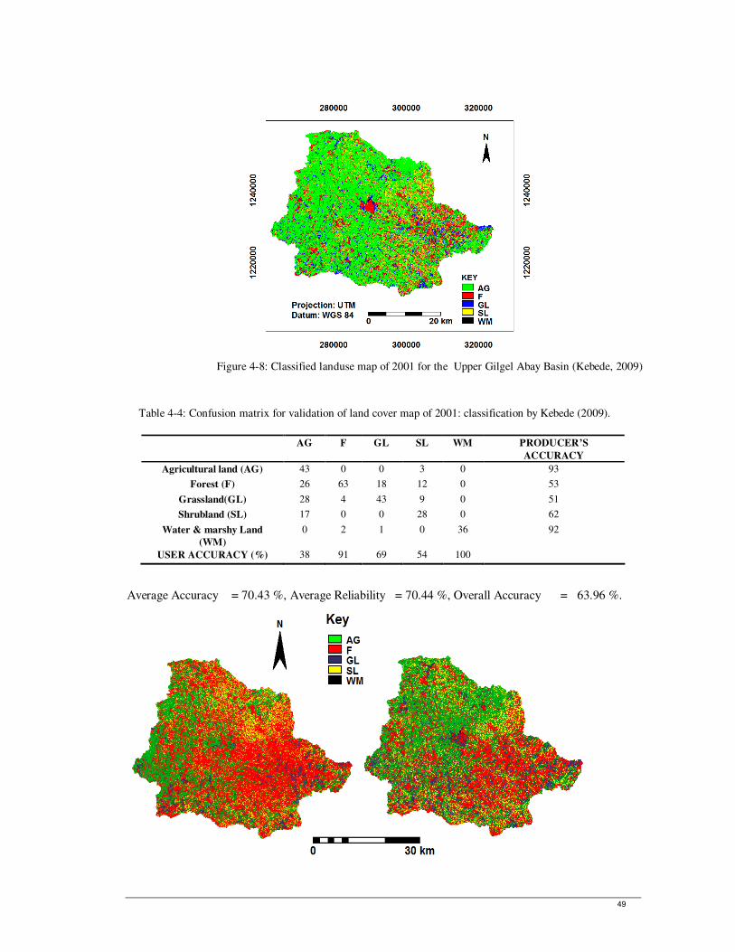
49
Figure 4-8: Classified landuse map of 2001 for the Upper Gilgel Abay Basin (Kebede, 2009)
Table 4-4: Confusion matrix for validation of land cover map of 2001: classification by Kebede (2009).
Average Accuracy = 70.43 %, Average Reliability = 70.44 %, Overall Accuracy = 63.96 %.
AG F GL SL WM PRODUCER’S
ACCURACY
Agricultural land (AG) 43 0 0 3 0 93
Forest (F) 26 63 18 12 0 53
Grassland(GL) 28 4 43 9 0 51
Shrubland (SL) 17 0 0 28 0 62
Water & marshy Land
(WM)
0 2 1 0 36 92
USER ACCURACY (%) 38 91 69 54 100
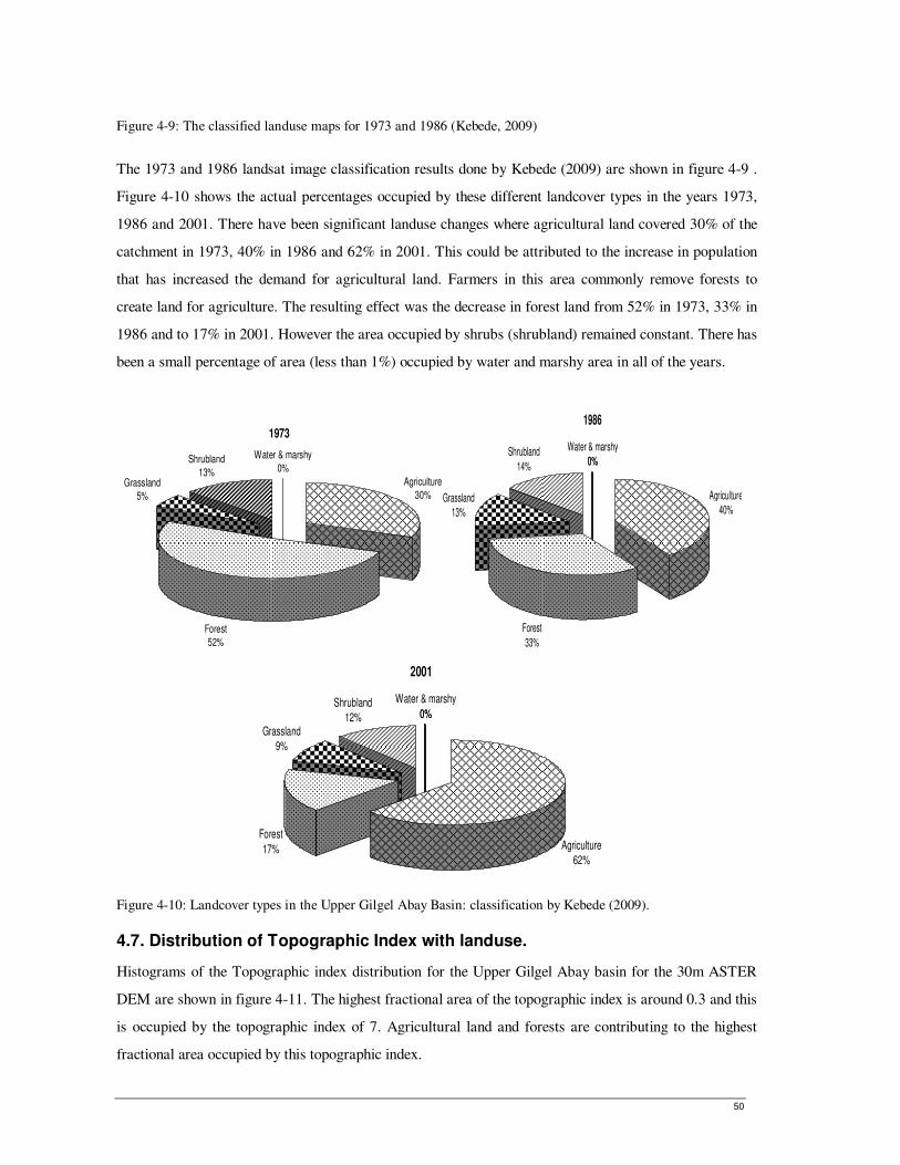
50
Figure 4-9: The classified landuse maps for 1973 and 1986 (Kebede, 2009)
The 1973 and 1986 landsat image classification results done by Kebede (2009) are shown in figure 4-9 .
Figure 4-10 shows the actual percentages occupied by these different landcover types in the years 1973,
1986 and 2001. There have been significant landuse changes where agricultural land covered 30% of the
catchment in 1973, 40% in 1986 and 62% in 2001. This could be attributed to the increase in population
that has increased the demand for agricultural land. Farmers in this area commonly remove forests to
create land for agriculture. The resulting effect was the decrease in forest land from 52% in 1973, 33% in
1986 and to 17% in 2001. However the area occupied by shrubs (shrubland) remained constant. There has
been a small percentage of area (less than 1%) occupied by water and marshy area in all of the years.
1973
Agriculture
30%
Forest
52%
Shrubland
13%Grassland
5%
Water & marshy
0%
1986
Agriculture
40%
Forest
33%
Grassland
13%
Shrubland
14%
Water & marshy
0%0%
2001
Agriculture
62%
Forest
17%
Grassland
9%
Shrubland
12%
Water & marshy
0%0%
Figure 4-10: Landcover types in the Upper Gilgel Abay Basin: classification by Kebede (2009).
4.7. Distribution of Topographic Index with landuse.
Histograms of the Topographic index distribution for the Upper Gilgel Abay basin for the 30m ASTER
DEM are shown in figure 4-11. The highest fractional area of the topographic index is around 0.3 and this
is occupied by the topographic index of 7. Agricultural land and forests are contributing to the highest
fractional area occupied by this topographic index.
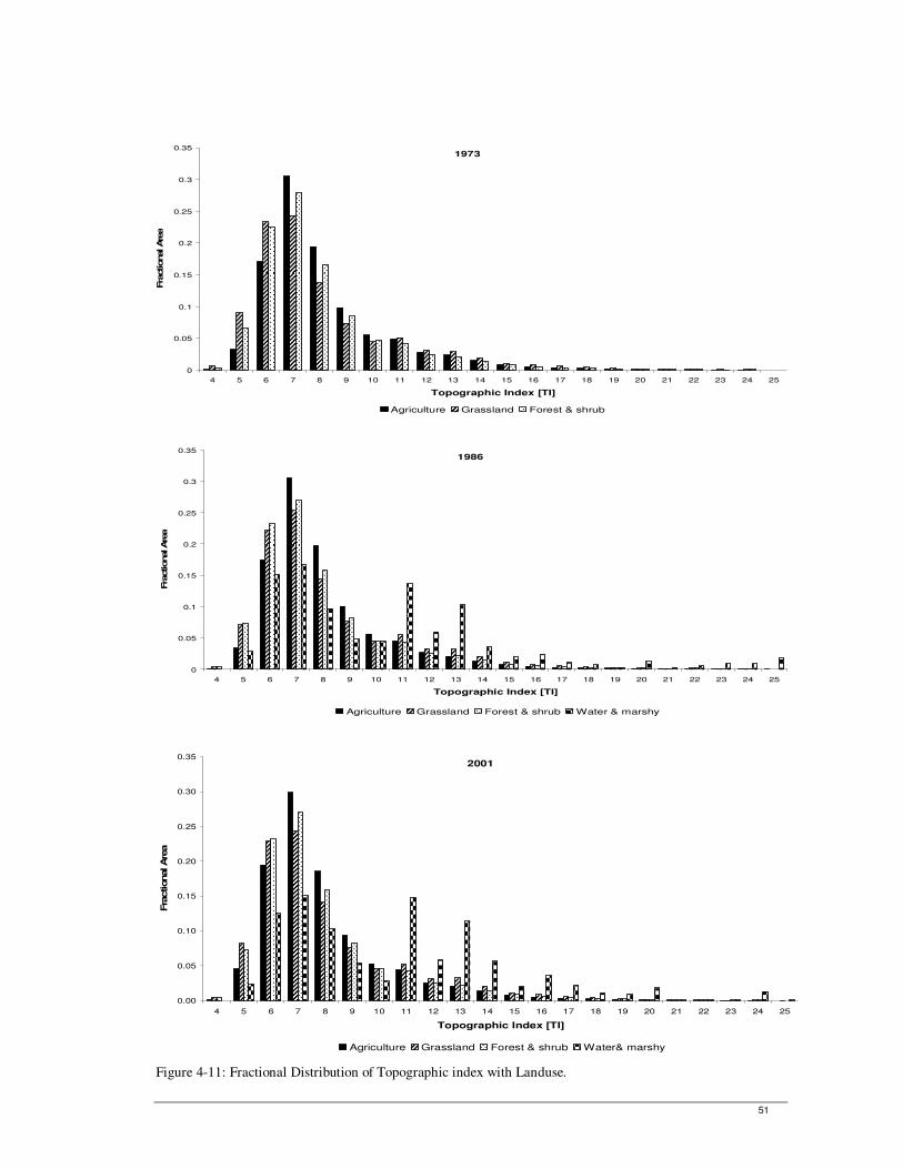
51
1973
0
0.05
0.1
0.15
0.2
0.25
0.3
0.35
4 5 6 7 8 9 10 11 12 13 14 15 16 17 18 19 20 21 22 23 24 25
Topographic Index [TI]
Fra
ctional Are
a
Agriculture Grassland Forest & shrub
1986
0
0.05
0.1
0.15
0.2
0.25
0.3
0.35
4 5 6 7 8 9 10 11 12 13 14 15 16 17 18 19 20 21 22 23 24 25
Topographic Index [TI]
Fra
ctional Are
a
Agriculture Grassland Forest & shrub Water & marshy
2001
0.00
0.05
0.10
0.15
0.20
0.25
0.30
0.35
4 5 6 7 8 9 10 11 12 13 14 15 16 17 18 19 20 21 22 23 24 25
Topographic Index [TI]
Fra
ctional Are
a
Agriculture Grassland Forest & shrub Water& marshy
Figure 4-11: Fractional Distribution of Topographic index with Landuse.
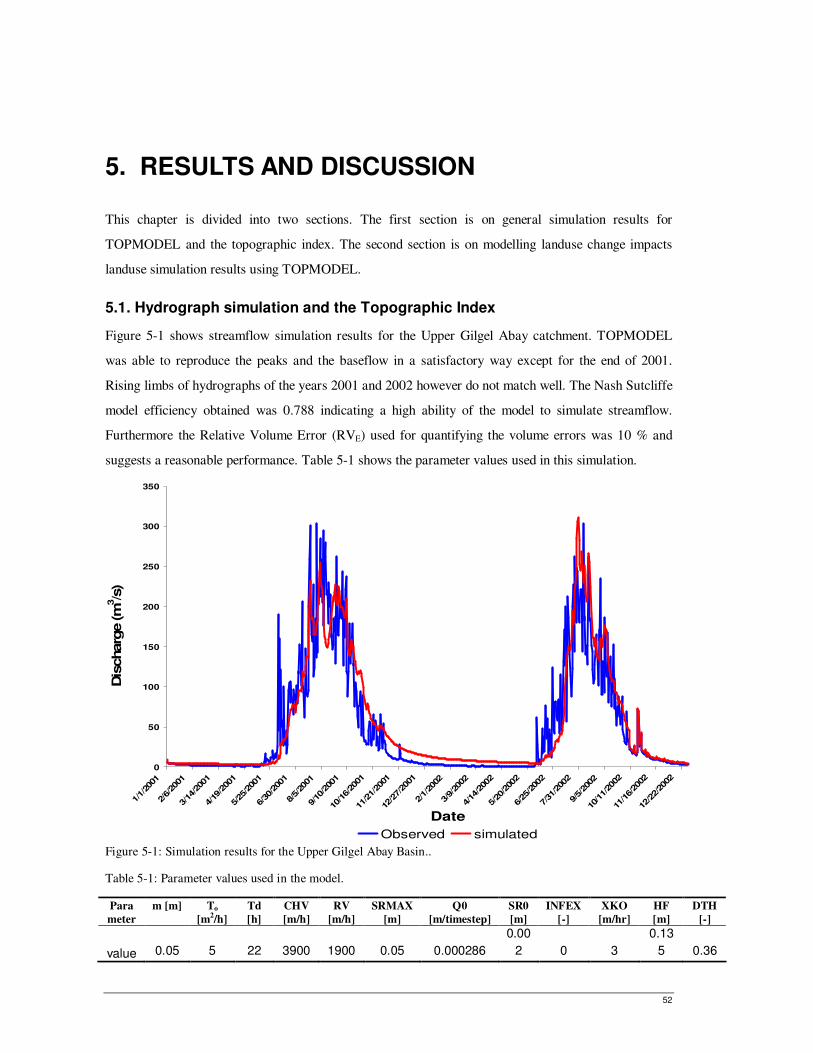
52
5. RESULTS AND DISCUSSION
This chapter is divided into two sections. The first section is on general simulation results for
TOPMODEL and the topographic index. The second section is on modelling landuse change impacts
landuse simulation results using TOPMODEL.
5.1. Hydrograph simulation and the Topographic Index
Figure 5-1 shows streamflow simulation results for the Upper Gilgel Abay catchment. TOPMODEL
was able to reproduce the peaks and the baseflow in a satisfactory way except for the end of 2001.
Rising limbs of hydrographs of the years 2001 and 2002 however do not match well. The Nash Sutcliffe
model efficiency obtained was 0.788 indicating a high ability of the model to simulate streamflow.
Furthermore the Relative Volume Error (RVE) used for quantifying the volume errors was 10 % and
suggests a reasonable performance. Table 5-1 shows the parameter values used in this simulation.
0
50
100
150
200
250
300
350
1/1/20
01
2/6/20
01
3/14
/200
1
4/19
/200
1
5/25
/200
1
6/30
/200
1
8/5/20
01
9/10
/200
1
10/16/20
01
11/21/20
01
12/27/20
01
2/1/20
02
3/9/20
02
4/14
/200
2
5/20
/200
2
6/25
/200
2
7/31
/200
2
9/5/20
02
10/11/20
02
11/16/20
02
12/22/20
02
Date
Dis
charg
e (m
3/s
)
Observed simulated Figure 5-1: Simulation results for the Upper Gilgel Abay Basin..
Table 5-1: Parameter values used in the model.
Para
meter
m [m] To
[m2/h]
Td
[h]
CHV
[m/h]
RV
[m/h]
SRMAX
[m]
Q0
[m/timestep]
SR0
[m]
INFEX
[-]
XKO
[m/hr]
HF
[m]
DTH
[-]
value 0.05 5 22 3900 1900 0.05 0.000286
0.00
2 0 3
0.13
5 0.36
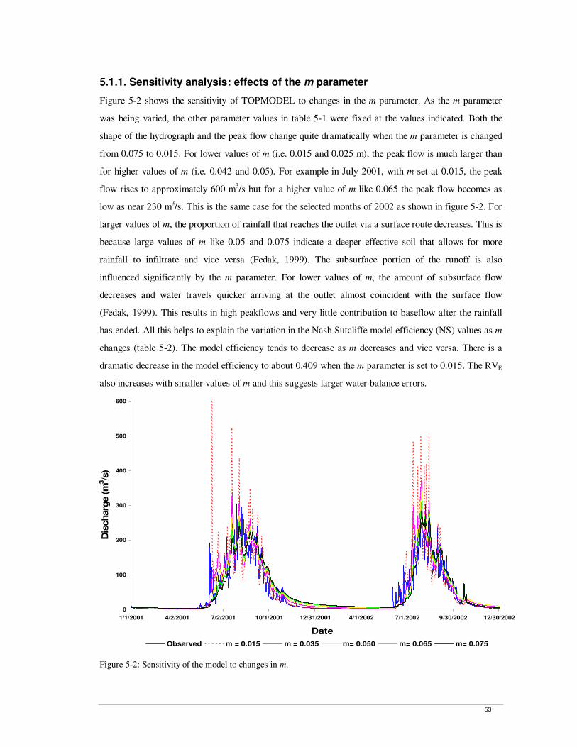
53
5.1.1. Sensitivity analysis: effects of the m parameter
Figure 5-2 shows the sensitivity of TOPMODEL to changes in the m parameter. As the m parameter
was being varied, the other parameter values in table 5-1 were fixed at the values indicated. Both the
shape of the hydrograph and the peak flow change quite dramatically when the m parameter is changed
from 0.075 to 0.015. For lower values of m (i.e. 0.015 and 0.025 m), the peak flow is much larger than
for higher values of m (i.e. 0.042 and 0.05). For example in July 2001, with m set at 0.015, the peak
flow rises to approximately 600 m3/s but for a higher value of m like 0.065 the peak flow becomes as
low as near 230 m3/s. This is the same case for the selected months of 2002 as shown in figure 5-2. For
larger values of m, the proportion of rainfall that reaches the outlet via a surface route decreases. This is
because large values of m like 0.05 and 0.075 indicate a deeper effective soil that allows for more
rainfall to infiltrate and vice versa (Fedak, 1999). The subsurface portion of the runoff is also
influenced significantly by the m parameter. For lower values of m, the amount of subsurface flow
decreases and water travels quicker arriving at the outlet almost coincident with the surface flow
(Fedak, 1999). This results in high peakflows and very little contribution to baseflow after the rainfall
has ended. All this helps to explain the variation in the Nash Sutcliffe model efficiency (NS) values as m
changes (table 5-2). The model efficiency tends to decrease as m decreases and vice versa. There is a
dramatic decrease in the model efficiency to about 0.409 when the m parameter is set to 0.015. The RVE
also increases with smaller values of m and this suggests larger water balance errors.
0
100
200
300
400
500
600
1/1/2001 4/2/2001 7/2/2001 10/1/2001 12/31/2001 4/1/2002 7/1/2002 9/30/2002 12/30/2002
Date
Dis
charg
e (m
3/s
)
Observed m = 0.015 m = 0.035 m= 0.050 m= 0.065 m= 0.075
Figure 5-2: Sensitivity of the model to changes in m.
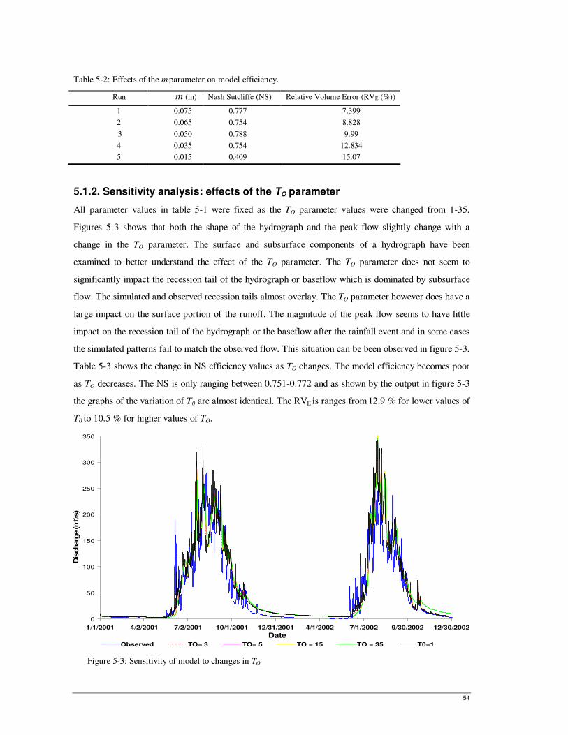
54
Table 5-2: Effects of the m parameter on model efficiency.
Run m (m) Nash Sutcliffe (NS) Relative Volume Error (RVE (%))
1 0.075 0.777 7.399
2 0.065 0.754 8.828
3 0.050 0.788 9.99
4 0.035 0.754 12.834
5 0.015 0.409 15.07
5.1.2. Sensitivity analysis: effects of the TO parameter
All parameter values in table 5-1 were fixed as the TO parameter values were changed from 1-35.
Figures 5-3 shows that both the shape of the hydrograph and the peak flow slightly change with a
change in the TO parameter. The surface and subsurface components of a hydrograph have been
examined to better understand the effect of the TO parameter. The TO parameter does not seem to
significantly impact the recession tail of the hydrograph or baseflow which is dominated by subsurface
flow. The simulated and observed recession tails almost overlay. The TO parameter however does have a
large impact on the surface portion of the runoff. The magnitude of the peak flow seems to have little
impact on the recession tail of the hydrograph or the baseflow after the rainfall event and in some cases
the simulated patterns fail to match the observed flow. This situation can be been observed in figure 5-3.
Table 5-3 shows the change in NS efficiency values as TO changes. The model efficiency becomes poor
as TO decreases. The NS is only ranging between 0.751-0.772 and as shown by the output in figure 5-3
the graphs of the variation of T0 are almost identical. The RVE is ranges from 12.9 % for lower values of
T0 to 10.5 % for higher values of TO.
0
50
100
150
200
250
300
350
1/1/2001 4/2/2001 7/2/2001 10/1/2001 12/31/2001 4/1/2002 7/1/2002 9/30/2002 12/30/2002
Date
Dis
charg
e (m
3/s
)
Observed TO= 3 TO= 5 TO = 15 TO = 35 T0=1
Figure 5-3: Sensitivity of model to changes in TO
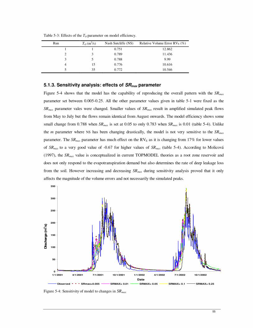
55
Table 5-3: Effects of the TO parameter on model efficiency.
Run TO (m2/s) Nash Sutcliffe (NS) Relative Volume Error RVE (%)
1 1 0.751 12.862
2 3 0.789 11.436
3 5 0.788 9.99
4 15 0.776 10.616
5 35 0.772 10.546
5.1.3. Sensitivity analysis: effects of SRmax parameter
Figure 5-4 shows that the model has the capability of reproducing the overall pattern with the SRmax
parameter set between 0.005-0.25. All the other parameter values given in table 5-1 were fixed as the
SRmax parameter vales were changed. Smaller values of SRmax result in amplified simulated peak flows
from May to July but the flows remain identical from August onwards. The model efficiency shows some
small change from 0.788 when SRmax is set at 0.05 to only 0.783 when SRmax is 0.01 (table 5-4). Unlike
the m parameter where NS has been changing drastically, the model is not very sensitive to the SRmax
parameter. The SRmax parameter has much effect on the RVE as it is changing from 17% for lower values
of SRmax to a very good value of -0.67 for higher values of SRmax (table 5-4). According to Molicová
(1997), the SRmax value is conceptualized in current TOPMODEL theories as a root zone reservoir and
does not only respond to the evapotranspiration demand but also determines the rate of deep leakage loss
from the soil. However increasing and decreasing SRmax during sensitivity analysis proved that it only
affects the magnitude of the volume errors and not necessarily the simulated peaks.
0
50
100
150
200
250
300
350
1/1/2001 4/1/2001 7/1/2001 10/1/2001 1/1/2002 4/1/2002 7/1/2002 10/1/2002
Date
Dis
charg
e (m
3/s
)
Observed SRmax=0.005 SRMAX= 0.01 SRMAX= 0.05 SRMAX= 0.1 SRMAX= 0.25
Figure 5-4: Sensitivity of model to changes in SRmax
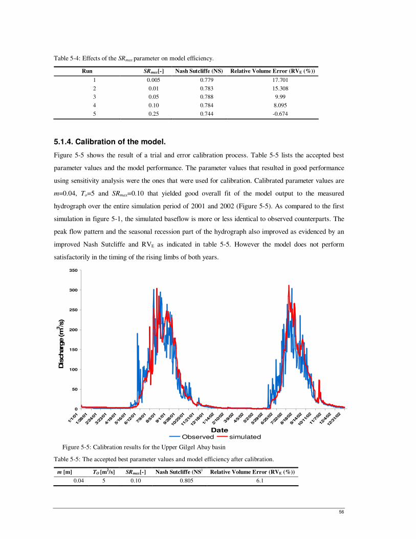
56
Table 5-4: Effects of the SRmax parameter on model efficiency.
Run SRmax[-] Nash Sutcliffe (NS) Relative Volume Error (RVE (%))
1 0.005 0.779 17.701
2 0.01 0.783 15.308
3 0.05 0.788 9.99
4 0.10 0.784 8.095
5 0.25 0.744 -0.674
5.1.4. Calibration of the model.
Figure 5-5 shows the result of a trial and error calibration process. Table 5-5 lists the accepted best
parameter values and the model performance. The parameter values that resulted in good performance
using sensitivity analysis were the ones that were used for calibration. Calibrated parameter values are
m=0.04, To=5 and SRmax=0.10 that yielded good overall fit of the model output to the measured
hydrograph over the entire simulation period of 2001 and 2002 (Figure 5-5). As compared to the first
simulation in figure 5-1, the simulated baseflow is more or less identical to observed counterparts. The
peak flow pattern and the seasonal recession part of the hydrograph also improved as evidenced by an
improved Nash Sutcliffe and RVE as indicated in table 5-5. However the model does not perform
satisfactorily in the timing of the rising limbs of both years.
0
50
100
150
200
250
300
350
1/1/01
1/28
/01
2/24
/01
3/23
/01
4/19
/01
5/16
/01
6/12
/01
7/9/01
8/5/01
9/1/01
9/28
/01
10/25/01
11/21/01
12/18/01
1/14
/02
2/10
/02
3/9/02
4/5/02
5/2/02
5/29
/02
6/25
/02
7/22
/02
8/18
/02
9/14
/02
10/11/02
11/7/02
12/4/02
12/31/02
Date
Dis
charg
e (m
3/s
)
Observed simulated
Figure 5-5: Calibration results for the Upper Gilgel Abay basin
Table 5-5: The accepted best parameter values and model efficiency after calibration.
m [m] TO [m2/s] SRmax[-] Nash Sutcliffe (NS) Relative Volume Error (RVE (%))
0.04 5 0.10 0.805 6.1
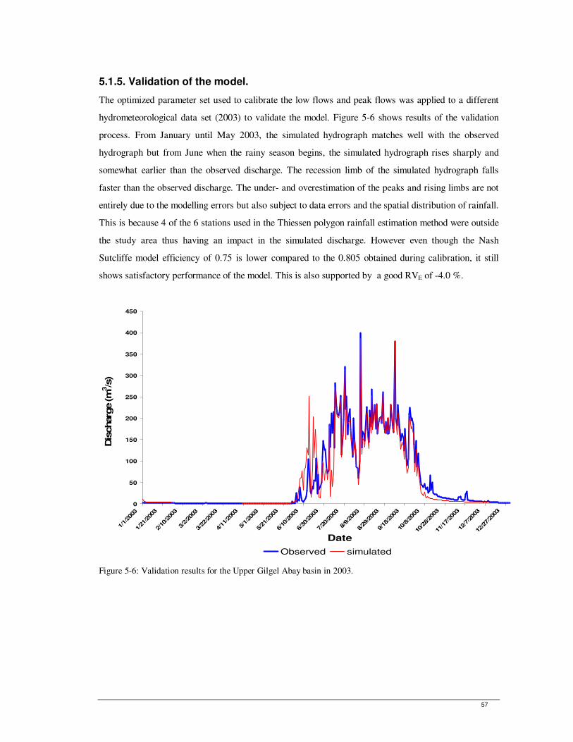
57
5.1.5. Validation of the model.
The optimized parameter set used to calibrate the low flows and peak flows was applied to a different
hydrometeorological data set (2003) to validate the model. Figure 5-6 shows results of the validation
process. From January until May 2003, the simulated hydrograph matches well with the observed
hydrograph but from June when the rainy season begins, the simulated hydrograph rises sharply and
somewhat earlier than the observed discharge. The recession limb of the simulated hydrograph falls
faster than the observed discharge. The under- and overestimation of the peaks and rising limbs are not
entirely due to the modelling errors but also subject to data errors and the spatial distribution of rainfall.
This is because 4 of the 6 stations used in the Thiessen polygon rainfall estimation method were outside
the study area thus having an impact in the simulated discharge. However even though the Nash
Sutcliffe model efficiency of 0.75 is lower compared to the 0.805 obtained during calibration, it still
shows satisfactory performance of the model. This is also supported by a good RVE of -4.0 %.
0
50
100
150
200
250
300
350
400
450
1/1/20
03
1/21
/200
3
2/10
/200
3
3/2/20
03
3/22
/200
3
4/11
/200
3
5/1/20
03
5/21
/200
3
6/10
/200
3
6/30
/200
3
7/20
/200
3
8/9/20
03
8/29
/200
3
9/18
/200
3
10/8/200
3
10/28/20
03
11/17/20
03
12/7/200
3
12/27/20
03
Date
Dis
charg
e (m
3/s
)
Observed simulated
Figure 5-6: Validation results for the Upper Gilgel Abay basin in 2003.
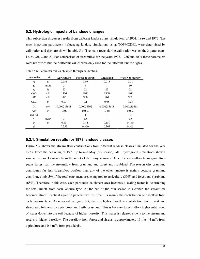
58
5.2. Hydrologic impacts of Landuse changes
This subsection discusses results from different landuse class simulations of 2001, 1986 and 1973. The
most important parameters influencing landuse simulations using TOPMODEL were determined by
calibration and they are shown in table 5-6. The main focus during calibration was on the 3 parameters:
i.e. m, SRmax and Ks. For comparison of streamflow for the years 1973, 1986 and 2001 these parameters
were not varied but their different values were only used for the different landuse types.
Table 5-6: Parameter values obtained through calibration.
Parameter Unit Agriculture Forest & shrub Grassland Water & marshy
m m 0.035 0.05 0.015 0.01
To m2/h 3 5 1 10
td h 22 22 22 22
CHV m/h 1900 1900 1900 1900
RV m/h 900 900 900 900
SRmax m 0.07 0.1 0.05 0.23
Qo m/h 0.000285618 0.00028562 0.000285618 0.000285618
SR0 m 0.002 0.002 0.002 0.002
INFEX - 1 1 1 0
Ks m/hr 3 2.5 1 0.5
Ψf m 0.13 0.14 0.159 0.160
Θ - 0.355 0.360 0.365 0.365
5.2.1. Simulation results for 1973 landuse classes
Figure 5-7 shows the stream flow contributions from different landuse classes simulated for the year
1973. From the beginning of 1973 up to mid May (dry season), all 3 hydrograph simulations show a
similar pattern. However from the onset of the rainy season in June, the streamflow from agriculture
peaks faster than the streamflow from grassland and forest and shrubland. The reason why grassland
contributes far less streamflow outflow than any of the other landuse is mainly because grassland
contributes only 5% of the total catchment area compared to agriculture (30%) and forest and shrubland
(65%). Therefore in this case, each particular catchment area becomes a scaling factor in determining
the total runoff from each landuse type. At the end of the rain season in October, the streamflow
becomes almost identical again in pattern and this time it is mainly the contribution of baseflow from
each landuse type. As observed in figure 5-7, there is higher baseflow contribution from forest and
shrubland, followed by agriculture and lastly grassland. This is because forests allow higher infiltration
of water down into the soil because of higher porosity. This water is released slowly to the stream and
results in higher baseflow. The baseflow from forest and shrubs is approximately 11m3/s, 4 m
3/s from
agriculture and 0.4 m3/s from grasslands.
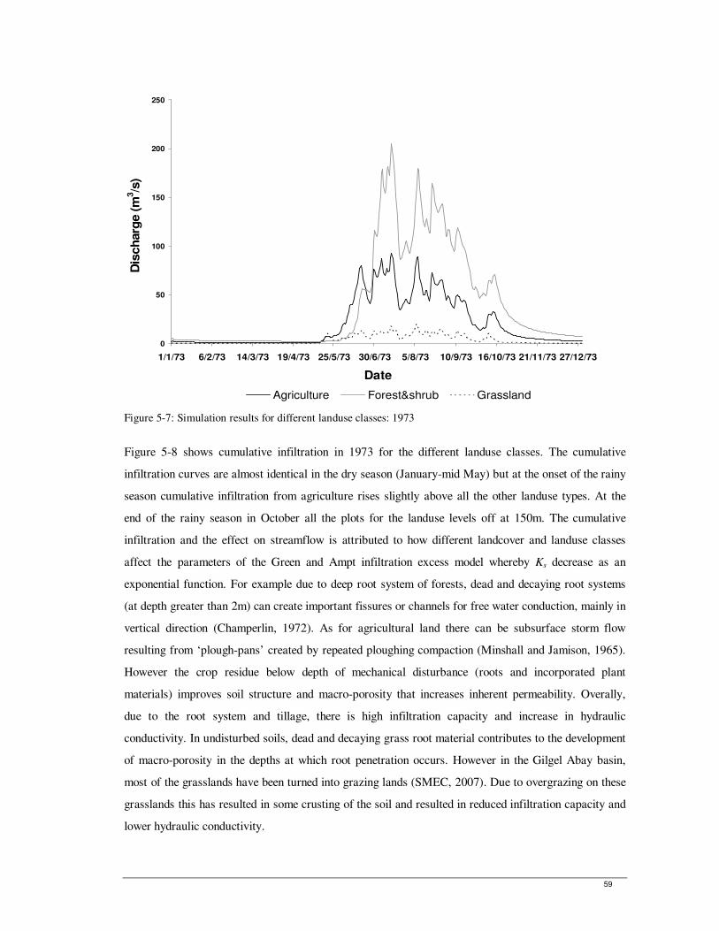
59
0
50
100
150
200
250
1/1/73 6/2/73 14/3/73 19/4/73 25/5/73 30/6/73 5/8/73 10/9/73 16/10/73 21/11/73 27/12/73
Date
Dis
ch
arg
e (
m3/s
)
Agriculture Forest&shrub Grassland
Figure 5-7: Simulation results for different landuse classes: 1973
Figure 5-8 shows cumulative infiltration in 1973 for the different landuse classes. The cumulative
infiltration curves are almost identical in the dry season (January-mid May) but at the onset of the rainy
season cumulative infiltration from agriculture rises slightly above all the other landuse types. At the
end of the rainy season in October all the plots for the landuse levels off at 150m. The cumulative
infiltration and the effect on streamflow is attributed to how different landcover and landuse classes
affect the parameters of the Green and Ampt infiltration excess model whereby Ks decrease as an
exponential function. For example due to deep root system of forests, dead and decaying root systems
(at depth greater than 2m) can create important fissures or channels for free water conduction, mainly in
vertical direction (Champerlin, 1972). As for agricultural land there can be subsurface storm flow
resulting from ‘plough-pans’ created by repeated ploughing compaction (Minshall and Jamison, 1965).
However the crop residue below depth of mechanical disturbance (roots and incorporated plant
materials) improves soil structure and macro-porosity that increases inherent permeability. Overally,
due to the root system and tillage, there is high infiltration capacity and increase in hydraulic
conductivity. In undisturbed soils, dead and decaying grass root material contributes to the development
of macro-porosity in the depths at which root penetration occurs. However in the Gilgel Abay basin,
most of the grasslands have been turned into grazing lands (SMEC, 2007). Due to overgrazing on these
grasslands this has resulted in some crusting of the soil and resulted in reduced infiltration capacity and
lower hydraulic conductivity.
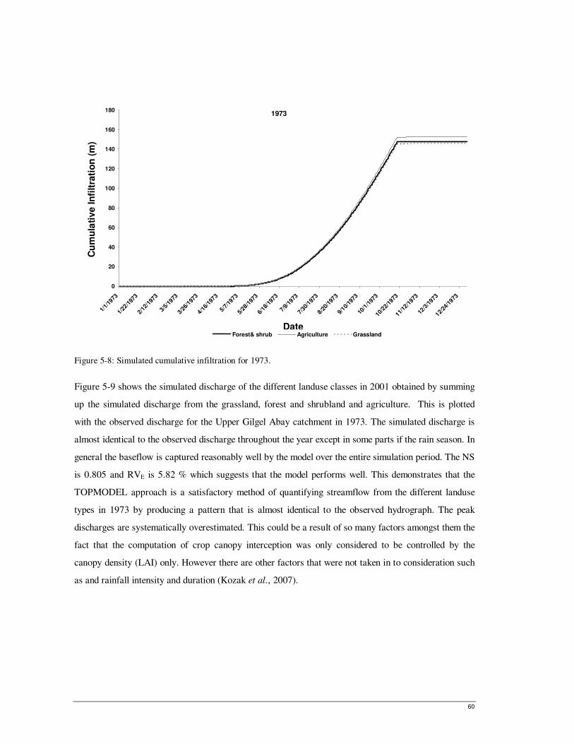
60
1973
0
20
40
60
80
100
120
140
160
180
1/1/
1973
1/22
/197
3
2/12
/197
3
3/5/
1973
3/26
/197
3
4/16/
1973
5/7/1
973
5/28
/197
3
6/18
/197
3
7/9/
1973
7/30
/197
3
8/20/
1973
9/10/
1973
10/1
/197
3
10/2
2/19
73
11/1
2/197
3
12/3
/1973
12/24
/1973
Date
Cu
mu
lati
ve In
filt
rati
on
(m
)
Forest& shrub Agriculture Grassland
Figure 5-8: Simulated cumulative infiltration for 1973.
Figure 5-9 shows the simulated discharge of the different landuse classes in 2001 obtained by summing
up the simulated discharge from the grassland, forest and shrubland and agriculture. This is plotted
with the observed discharge for the Upper Gilgel Abay catchment in 1973. The simulated discharge is
almost identical to the observed discharge throughout the year except in some parts if the rain season. In
general the baseflow is captured reasonably well by the model over the entire simulation period. The NS
is 0.805 and RVE is 5.82 % which suggests that the model performs well. This demonstrates that the
TOPMODEL approach is a satisfactory method of quantifying streamflow from the different landuse
types in 1973 by producing a pattern that is almost identical to the observed hydrograph. The peak
discharges are systematically overestimated. This could be a result of so many factors amongst them the
fact that the computation of crop canopy interception was only considered to be controlled by the
canopy density (LAI) only. However there are other factors that were not taken in to consideration such
as and rainfall intensity and duration (Kozak et al., 2007).
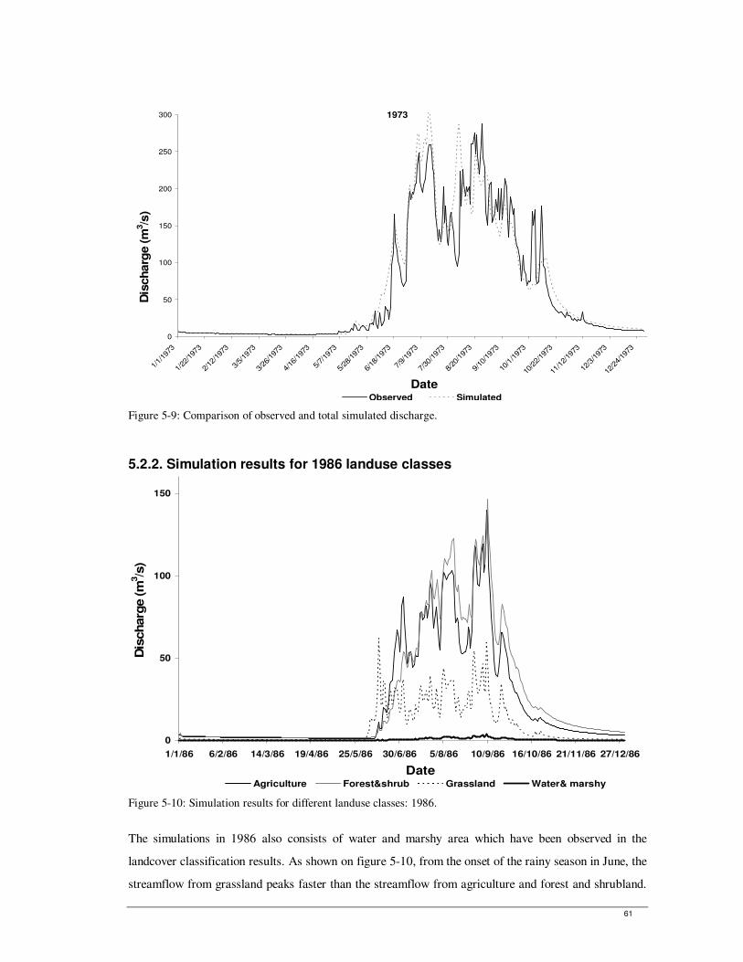
61
1973
0
50
100
150
200
250
300
1/1/
1973
1/22
/197
3
2/12
/197
3
3/5/
1973
3/26
/197
3
4/16
/197
3
5/7/
1973
5/28
/197
3
6/18
/197
3
7/9/
1973
7/30
/197
3
8/20
/197
3
9/10
/197
3
10/1
/197
3
10/22/
1973
11/12/19
73
12/3
/197
3
12/24/
1973
Date
Dis
charg
e (m
3/s
)
Observed Simulated
Figure 5-9: Comparison of observed and total simulated discharge.
5.2.2. Simulation results for 1986 landuse classes
0
50
100
150
1/1/86 6/2/86 14/3/86 19/4/86 25/5/86 30/6/86 5/8/86 10/9/86 16/10/86 21/11/86 27/12/86
Date
Dis
charg
e (m
3/s
)
Agriculture Forest&shrub Grassland Water& marshy
Figure 5-10: Simulation results for different landuse classes: 1986.
The simulations in 1986 also consists of water and marshy area which have been observed in the
landcover classification results. As shown on figure 5-10, from the onset of the rainy season in June, the
streamflow from grassland peaks faster than the streamflow from agriculture and forest and shrubland.
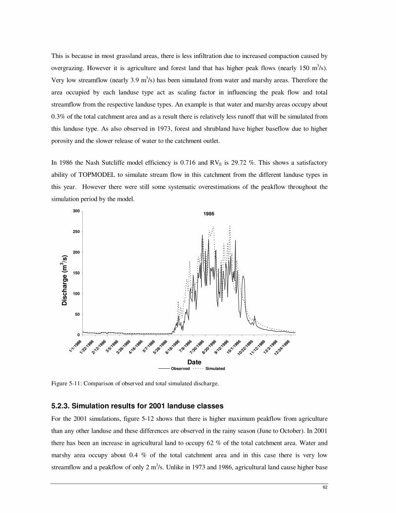
62
This is because in most grassland areas, there is less infiltration due to increased compaction caused by
overgrazing. However it is agriculture and forest land that has higher peak flows (nearly 150 m3/s).
Very low streamflow (nearly 3.9 m3/s) has been simulated from water and marshy areas. Therefore the
area occupied by each landuse type act as scaling factor in influencing the peak flow and total
streamflow from the respective landuse types. An example is that water and marshy areas occupy about
0.3% of the total catchment area and as a result there is relatively less runoff that will be simulated from
this landuse type. As also observed in 1973, forest and shrubland have higher baseflow due to higher
porosity and the slower release of water to the catchment outlet.
In 1986 the Nash Sutcliffe model efficiency is 0.716 and RVE is 29.72 %. This shows a satisfactory
ability of TOPMODEL to simulate stream flow in this catchment from the different landuse types in
this year. However there were still some systematic overestimations of the peakflow throughout the
simulation period by the model.
1986
0
50
100
150
200
250
300
1/1/
1986
1/22
/198
6
2/12/
1986
3/5/1
986
3/26
/198
6
4/16
/198
6
5/7/
1986
5/28
/1986
6/18/
1986
7/9/1
986
7/30/
1986
8/20
/1986
9/10/
1986
10/1
/198
6
10/2
2/19
86
11/12
/198
6
12/3/
1986
12/2
4/198
6
Date
Dis
ch
arg
e (
m3/s
)
Observed Simulated
Figure 5-11: Comparison of observed and total simulated discharge.
5.2.3. Simulation results for 2001 landuse classes
For the 2001 simulations, figure 5-12 shows that there is higher maximum peakflow from agriculture
than any other landuse and these differences are observed in the rainy season (June to October). In 2001
there has been an increase in agricultural land to occupy 62 % of the total catchment area. Water and
marshy area occupy about 0.4 % of the total catchment area and in this case there is very low
streamflow and a peakflow of only 2 m3/s. Unlike in 1973 and 1986, agricultural land cause higher base
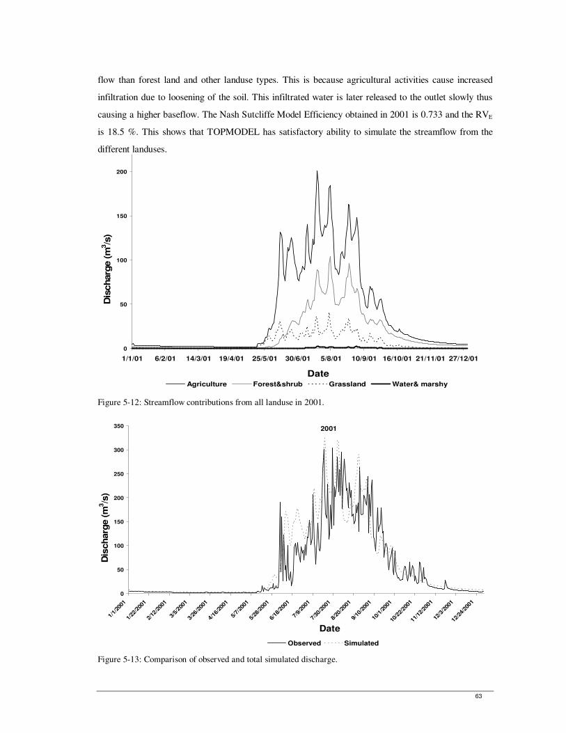
63
flow than forest land and other landuse types. This is because agricultural activities cause increased
infiltration due to loosening of the soil. This infiltrated water is later released to the outlet slowly thus
causing a higher baseflow. The Nash Sutcliffe Model Efficiency obtained in 2001 is 0.733 and the RVE
is 18.5 %. This shows that TOPMODEL has satisfactory ability to simulate the streamflow from the
different landuses.
0
50
100
150
200
1/1/01 6/2/01 14/3/01 19/4/01 25/5/01 30/6/01 5/8/01 10/9/01 16/10/01 21/11/01 27/12/01
Date
Dis
charg
e (m
3/s
)
Agriculture Forest&shrub Grassland Water& marshy
Figure 5-12: Streamflow contributions from all landuse in 2001.
2001
0
50
100
150
200
250
300
350
1/1/
2001
1/22
/200
1
2/12
/200
1
3/5/
2001
3/26
/200
1
4/16
/200
1
5/7/
2001
5/28
/200
1
6/18
/200
1
7/9/
2001
7/30
/200
1
8/20
/200
1
9/10
/200
1
10/1
/200
1
10/2
2/20
01
11/1
2/20
01
12/3
/200
1
12/2
4/20
01
Date
Dis
charg
e (m
3/s
)
Observed Simulated
Figure 5-13: Comparison of observed and total simulated discharge.
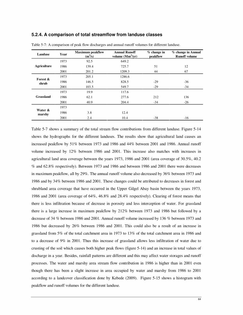
64
5.2.4. A comparison of total streamflow from landuse classes
Table 5-7: A comparison of peak flow discharges and annual runoff volumes for different landuse.
Landuse Year Maximum peakflow
(m3/s)
Annual Runoff
volume (Mm3/yr)
% change in
peakflow
% change in Annual
Runoff volume
1973 92.5 649.2
1986 139.4 725.7 51 12 Agriculture
2001 201.2 1209.3 44 67
1973 205.1 1286.6
1986 146.5 828.5 -29 -36 Forest &
shrub 2001 103.5 549.7 -29 -34
1973 19.9 117.6
1986 62.1 277.6 212 136 Grassland
2001 40.9 204.4 -34 -26
1973
1986 3.8 12.4 Water &
marshy 2001 2.4 10.4 -38 -16
Table 5-7 shows a summary of the total stream flow contributions from different landuse. Figure 5-14
shows the hydrographs for the different landuses. The results show that agricultural land causes an
increased peakflow by 51% between 1973 and 1986 and 44% between 2001 and 1986. Annual runoff
volume increased by 12% between 1986 and 2001. This increase also matches with increases in
agricultural land area coverage between the years 1973, 1986 and 2001 (area coverage of 30.5%, 40.2
% and 62.8% respectively). Between 1973 and 1986 and between 1986 and 2001 there were decreases
in maximum peakflow, all by 29%. The annual runoff volume also decreased by 36% between 1973 and
1986 and by 34% between 1986 and 2001. These changes could be attributed to decreases in forest and
shrubland area coverage that have occurred in the Upper Gilgel Abay basin between the years 1973,
1986 and 2001 (area coverage of 64%, 46.8% and 28.4% respectively). Clearing of forest means that
there is less infiltration because of decrease in porosity and less interception of water. For grassland
there is a large increase in maximum peakflow by 212% between 1973 and 1986 but followed by a
decrease of 34 % between 1986 and 2001. Annual runoff volume increased by 136 % between 1973 and
1986 but decreased by 26% between 1986 and 2001. This could also be a result of an increase in
grassland from 5% of the total catchment area in 1973 to 13% of the total catchment area in 1986 and
to a decrease of 9% in 2001. Thus this increase of grassland allows less infiltration of water due to
crusting of the soil which causes both higher peak flows (figure 5-14) and an increase in total values of
discharge in a year. Besides, rainfall patterns are different and this may affect water storages and runoff
processes. The water and marshy area stream flow contribution in 1986 is higher than in 2001 even
though there has been a slight increase in area occupied by water and marshy from 1986 to 2001
according to a landcover classification done by Kebede (2009). Figure 5-15 shows a histogram with
peakflow and runoff volumes for the different landuse.
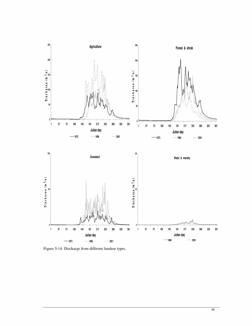
65
Agriculture
0
50
100
150
200
250
1 37 73 109 145 181 217 253 289 325 361
Julian day
Dis
ch
arg
e (
m3
/s)
1973 1986 2001
Forest & shrub
0
50
100
150
200
250
1 37 73 109 145 181 217 253 289 325 361
Julian day D
isc
ha
rge
(m
3/s
)1973 1986 2001
Grassland
0
50
100
1 37 73 109 145 181 217 253 289 325 361
Julian day
Dis
ch
arg
e (
m3
/s)
1973 1986 2001
Water & marshy
0
25
50
1 37 73 109 145 181 217 253 289 325 361
Julian day
Dis
ch
arg
e (
m3
/s)
1986 2001
Figure 5-14: Discharge from different landuse types.
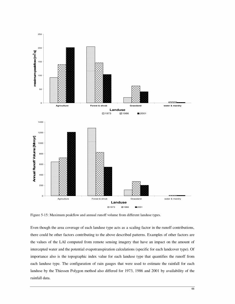
66
0
50
100
150
200
250
Agriculture Forest & shrub Grassland water & marshy
Landuse
maxim
um
peakflow
[m
3/s
]
1973 1986 2001
0
200
400
600
800
1000
1200
1400
Agriculture Forest & shrub Grassland water & marshy
Landuse
Annual R
unoff V
olu
me [M
m/y
r]
1973 1986 2001
Figure 5-15: Maximum peakflow and annual runoff volume from different landuse types.
Even though the area coverage of each landuse type acts as a scaling factor in the runoff contributions,
there could be other factors contributing to the above described patterns. Examples of other factors are
the values of the LAI computed from remote sensing imagery that have an impact on the amount of
intercepted water and the potential evapotranspiration calculations (specific for each landcover type). Of
importance also is the topographic index value for each landuse type that quantifies the runoff from
each landuse type. The configuration of rain gauges that were used to estimate the rainfall for each
landuse by the Thiessen Polygon method also differed for 1973, 1986 and 2001 by availability of the
rainfall data.
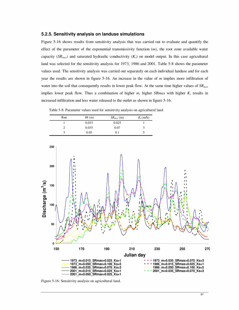
67
5.2.5. Sensitivity analysis on landuse simulations
Figure 5-16 shows results from sensitivity analysis that was carried out to evaluate and quantify the
effect of the parameter of the exponential transmissivity function (m), the root zone available water
capacity (SRmax) and saturated hydraulic conductivity (Ks) on model output. In this case agricultural
land was selected for the sensitivity analysis for 1973, 1986 and 2001. Table 5-8 shows the parameter
values used. The sensitivity analysis was carried out separately on each individual landuse and for each
year the results are shown in figure 5-16. An increase in the value of m implies more infiltration of
water into the soil that consequently results in lower peak flow. At the same time higher values of SRmax
implies lower peak flow. Thus a combination of higher m, higher SRmax with higher Ks results in
increased infiltration and less water released to the outlet as shown in figure 5-16.
Table 5-8: Parameter values used for sensitivity analysis on agricultural land
Run m (m) SRmax (m) Ks (m/h)
1 0.015 0.025 1
2 0.035 0.07 3
3 0.05 0.1 5
0
50
100
150
200
250
150 170 190 210 230 250 270
Julian day
Dis
ch
arg
e (
m3/s
)
1973_m=0.015_SRmax=0.025_Ks=1 1973_m=0.035_SRmax=0.070_Ks=31973_m=0.050_SRmax=0.100_Ks=5 1986_m=0.015_SRmax=0.025_Ks=11986_m=0.035_SRmax=0.070_Ks=3 1986_m=0.050_SRmax=0.100_Ks=52001_m=0.015_SRmax=0.025_Ks=1 2001_m=0.035_SRmax=0.070_Ks=32001_m=0.050_SRmax=0.025_Ks=1
Figure 5-16: Sensitivity analysis on agricultural land.
68
6. CONCLUSIONS AND RECOMMENDATIONS
6.1. Conclusions
• TOPMODEL was applied to simulate streamflow for the Upper Gilgel Abay River basin with
satisfactory results. This study demonstrated that the rainfall-runoff model can be extended
beyond its original design of using the topographic index for predicting local variations in water
table (Kirkby, 1975) to simulate impacts of land use change in a catchment with chosen
important parameters for any time period.
• The first research question was to assess whether land surface parameterization of
TOPMODEL can be achieved by the use of remote sensing. Land surface parameterization was
done in two parts, i.e. topographic indices and vegetation indices. In relation to topographic
indices, this study showed that it is important to integrate the various quantification abilities of
remote sensing together with the spatial data handling capabilities of GIS to process data for
hydrological modelling. Remote sensing was used for acquiring a fine resolution DEM which is
critical for the prediction of hillslope flow paths for distributed hydrological modeling.
Therefore in this study an ASTER 30m DEM was used for proper specification of flow
pathways that are important for computation of the topographic index > The results show that
the topographic index plays a dominant role in simulating streamflow in the Gilgel Abay River
basin. The second research question was on how well TOPMODEL can simulate streamflow in
the catchment. Results of calibration process showed a good Nash-Sutcliffe model efficiency
(NS) of 0.805 and a Relative Volume Error (RVE) of 6.1%. This suggests that TOPMODEL
simulates streamflow with good performance. The model was validated using a 2003 dataset
and a satisfactory model performance of NS=0.75, RVE= -4.0 % was also obtained.
• Landuse change is a major factor that alters the hydrological processes over a range of temporal
and spatial scales. Land surface parameterization was again successfully achieved through
derivation of vegetation parameters from remote sensing. Spectral vegetation indices such as the
Soil-Adjusted Vegetation Index (SAVI) and Leaf Area Index (LAI) were determined from
remote sensing imagery. Interception of precipitation from different landcover types was
calculated as a function of LAI. The rainfall runoff model has been further enhanced by the
aggregation of evapotranspiration according to specific vegetation cover using the crop
69
coefficient approach. Furthermore there was an addition of infiltration excess flow module of
the Green and Ampt model.
• The above helped to answer the research question on how the TOPMODEL structure could be
modified so that it can account for hydrologic impacts of landuse change. The most
approximate way of implementation of land-use in TOPMODEL was done by treatment of each
vegetation/landuse type as a ‘subcatchment’ through a GIS overlay of landuse types thus
creating a topographic index distribution for each landuse type. These were run separately with
specific landuse parameters. The areally weighted results were summed to get a total output
imitating having multiple subcatchments with different topographic index distributions.
• TOPMODEL was then applied to analyse streamflow contributions from different landuse
types, viz agriculture, grassland and forest and shrubs and water and marshy areas in the Upper
Gilgel Abay basin. Furthermore the model was used to assess how landuse change affects the
peakflow, baseflow and volume of runoff in the basin. Results have shown that there are
significant increases in maximum peakflow and annual runoff volume from agricultural land
over the period 1973-1986 and 1986-2001 which corresponds to increases in agricultural land
between the years 1973, 1986 and 2001 shown in figure 4-10. Over the same period of time,
forest and shrubland decreased in maximum peakflow and annual runoff volume which could
also be attributed to decreases in forest and shrubland land in the same period of time. For
grassland, increases in grassland resulted in significant increases in peakflow and volume runoff
between 1973 and 1986 but decreases in grassland resulted in decrease in maximum peakflow
and volume of runoff between 1986 and 2001. Annual runoff volume also increased by 136 %
between 1973 and 1986 but decreased by 26% between 1986 and 2001. The water and marshy
area stream flow contribution in 1986 has been found to be higher than in 2001 even though
there has been a slight increase in area occupied by water and marshy from between this period
of time. This demonstrated the significant local effects of landuse change on the hydrology of a
catchment. Furthermore this study has demonstrated that different landuse classes contribute to
significantly different streamflow. This confirmed the work by Chan et al. (2009) who also
observed that each land use type affect the runoff generation and concentration by altering
hydrological factors such as interception, infiltration and evaporation.
• It was however difficult to assess whether the streamflow contributions from each landuse are
accurate because the model is run separately for each landuse. Furthermore, on the actual
ground, a landuse class is not a hydrological subcatchment. The most approximate way was
70
through summing the simulated streamflow from the different land uses and by comparing with
the observed outflow for the whole catchment. This answer the research question on how the
combined discharge from different landuse classes compare to the observed discharge. The
following satisfactory model efficiencies were obtained on the comparison between the sum of
all landuse simulated discharge and the observed discharge at the outlet: 1973 (NS=0.81,
RVE=5.82); 1986 (NS=0.72, RVE=29.72) and 2001 (NS=0.73, RVE= 18.50). This
demonstrated that TOPMODEL performs with varying degrees of success in terms of matching
the observed surface runoff, peakflow and time to peak for all landuse classes.
6.2. Recommendations
• In order to improve the prediction of the spatial and temporal patterns of hydrological response
units in the Upper Gilgel Abay basin, more advanced coupling of TOPMODEL with remote
sensing data can further be done. In this study parameterization of TOPMODEL through
remote sensing has only been done for the land surface parameters. For further research,
complete parameterization of this rainfall runoff model can be achieved through remote sensing
to allow TOPMODEL to be applied in a fully distributed fashion. Thus satellite rainfall
blending techniques could provide effective means for calculating areal rainfall estimates.
Furthermore satellite based actual evapotranspiration estimation techniques could as well
provide effective means of estimating spatial and hyper-temporal evapotranspiration as inputs
to TOPMODEL.
• Manual calibration of the parameters in this study has been found to be both time consuming
and often erroneous. Automatic calibration using GLUE (Generalized Likelihood Uncertainty
Estimation) could improve simulation (Fisher J and Beven K.J, 1996). In GLUE, the parameter
sets are sampled randomly from physically reasonable ranges, often using uniform sampling
where there is no strong information about prior expectations of parameter values (Blazkova
and Beven, 2009). This can be a better approach for obtaining the values of parameters that
have been identified for sensitivity analysis in this study: m, To and SRmax. When applied to
landuse simulation this can be done also on additional parameters such as Ks.
• Another way of analysing the impacts of landuse change could be by creating land use
scenarios. Three hypothetical scenario targets can be prepared, namely agriculture,
deforestation and afforestation. Different scenarios can then be established by giving different
percentages of landcover and TOPMODEL run to simulate the impact responses.

71
• Future fieldwork campaigns also should measure hydraulic properties of soils since they play
an important role in movement of soil moisture from the land surface to the water table through
the unsaturated zone and, hence, affect the runoff and groundwater recharge processes. In this
regard, data generated through these field work investigations are expected to be useful for
modelling of unsaturated flow and to develop catchment based rainfall runoff relationships for
similar type of catchments.
• To allow for landuse change impact assessments using TOPMODEL, a number of additional
parameter values have been used to simulate infiltration by the Green and Ampt model. These
parameters are fixed at each run (a priori). However, the challenge that can be tackled in future
studies is that the effective root zone storage from tree types can change dramatically depending
on soil depths. This is the case mainly in forests and shrub land and future studies could focus
on how this could be implemented.
72
REFERENCES
Allen, R.G., Pereira, L.S., Raes, D. and Smith, M., 1998. Crop evapotranspiration- Guidelines for
computing crop water requirements, FAO Irrigation and Drainage Paper 56, FAO, ISBN 92-5-
104219-5. , Rome, Italy.
Ambroise, B., Beven, K. and Freer, J., 1996. Toward a generalization of the TOPMODEL concepts:
Topographic indices of hydrological similarity. Water Resources Research, 32(7): 2135-2145.
Ashenafi, S., 2007. Catchment modelling an preliminary application of isotopes for model validation in
Upper Blue Nile basin, Lake Tana, Ethiopia, MSc Thesis, UNESCO-IHE, Delft, The
Netherlands.
Band, L.E. et al., 1991. Forest ecosystem processes at the watershed scale: basis for distributed
simulation. Ecol. Modelling, 56: 171-196.
BCEOM, 1998. Abbay River Basin Integrated Development Master Plan Project, Environment, Part-3
Limnology Addis Ababa, Ethiopia.
Beven, K., 1984. Infiltration into a class of vertically non-uniform soils. Hydrol. Sci, 29(4): 425-434.
Beven, K., 1991. Spatially Distributed Modelling: Conceptual Approach to Runoff Prediction. In: D.S.
Bowles and P.E. O'Connell, Editors, Recent Advances in the Modelling of Hydrologic Systems,
Kluwer, Dordrecht (1991), pp. 373–387.
Beven, K., 1997a. "TOPMODEL: A CRITIQUE". Hydrological Processes, 11: 1069-1085.
Beven, K. and Freer, J., 2000. A dynamic TOPMODEL. Hydrological Processes, 15(10): 1993-2011.
Beven, K., Lamb, R., Quinn, P., Romanowicz, R. and Freer, J., 1995. TOPMODEL. In: Sing VP (Ed),
Computer Models of Watershed Hydrology. Water Resources Publications: 627-668, Colorado,
USA.
Beven, K.J., 1997b. Distributed hydrological modelling: Applications of the TOPMODEL concept. .
John Wiley and Sons Ltd, Chichester, U.K
Beven, K.J., 2001. Rainfall-Runoff Modelling The Primer. John Wiley & Sons, Lancaster.
Beven, K.J. and Kirkby, M.J., 1979. A physically based, variable contributing area model of basin
hydrology. Hydrological Sciences-Bulletin-des Sciences Hydrologiques, 24(1): 43-69.
Beven, K.J. and Wood, E.F., 1983. Catchment geomorphology and the dynamics of runoff contributing
areas. J. Hydrol., 65: 139±158.
Blazkova, S. and Beven, K.J., 2009. Uncertainty in flood estimation. Structure and Infrastructure
Engineering Maintenance, Management, Life-Cycle Design and Performance, 5 (4). pp. 325-
332.
Braden, H., 1985. Ein Energiehaushalts- uind verdunstungsmodell fur wasser- und
Stoffhaushaltsuntersuchungen landwirttschaftlich geutzter Einzugsgebiete. Mitteilungen
Deutsche Bodenkundliche Gesellschaft, 22: 294-299.
Champerlin, T.W., 1972. Interflow in the mountaneous forest soils of coastal British Columbia. In: D.
Slaymaker and H.J. McPherson (Editors), Mountain Geomorphology. Tantalus Research,
Vancouver, pp. 121-127.
Chen, Y., Xu, Y. and Yin, Y., 2009. Impacts of land use change scenarios on storm-runoff generation in
Xitiaoxi basin, China. Quaternary International, 208(1-2): 121-128.
Childs, E.C. and Bybordi, M., 1969. The vertical movement of water in. IUGG 282. stratified porous
material Water Resources Research.
Choudhury, B.J., Ahmed, N.U., Idso, S.B., Reginato, R.J. and Daughtry, C.S.T., 1994. Relations
between evaporation coefficients and vegetation indices studied by model simulations. Remote
Sensing of Environment, 50: 1-17.
Chrysoulakis, N., Abrams, M., Feidas, H. and Velianitis. D, 2004. Analysis of ASTER multispectral
stereo imagery to produce DEM and land cover databases for Greek Islands: the REALDEMS
project, EU-LAT Workshop on e-Environment, Brussels, Belgium 13-17 December.
D'Urso, G. and Santini, A., 1996. Advanced Procedures for the Management of Irrigation Systems.
Proceed. Intern. Workshop on Evapotranspiration and Irrig. Scheduling, ASAE, USA.
73
Daughtry, C.S.T., Gallo, K.P., Goward, S.N., Prince, S.D. and Kustas, W.P., 1992. Spectral estimates
of absorbed radiation and phytomass production in corn and soybean canopies Remote Sensing
of Environment, 39: 141-152.
Deginet, M.D., 2008. Land surface representation for regional rainfall - modelling, Upper Blue Nile
basin, Ethiopia, MSc Thesis, ITC, Enschede, 64 pp.
Dunne, T., 1978. Field studies of hillslope flow processes. In: M.J. Kikby (Editor), Hillslope
Hydrology. Wiley, London, pp. 227-294.
Famiglietti, J.S. and Wood, E.F., 1995. Multiscale modeling of spatially variable water and energy
balance processes. Water Resour. Res., 30(11): 3061–3078.
Fedak, R., 1999. Effect of Spatial Scale on Hydrologic Modeling in a Headwater Catchment, MSc
Thesis, Virginia Polytechnic Institute and State University, Virginia, USA.
Fisher J and Beven K.J, 1996. Modelling of stream flow at Slapton Wood using TOPMODEL within an
uncertainty estimation framework. Field Studies 8: 577-584.
Garbrecht, J. and Martz, L.W., 1999. Digital elevation model issues in water resources modeling. In:
Proceedings from invited water resources sessions, ESRI international user conference, pp. 1-
17.
Gash, J.H.C., 1979. An analytical model of rainfall interception by forests. Q. J. R. Meteor. Soc, 105:
43-55.
Gash, J.H.C., Lloyd, C.R. and Lachaud, G., 1995. Estimating sparse forest rainfall interception with an
analytical model Journal of Hydrology, 170: 79-86.
Green, W.H. and Ampt, G., 1911. Studies of soil physics, part I - The flow of air and water through
soils J. Ag. Sci., 4: 1-24.
Gunter, A., Uhlenbrook. S, Sibert, J. and C, L., 1999. Multi-criterial validation of TOPMODEL in a
mountaneous catchment. Hydrological Processes, 13: 1603-1620.
Hengl, T., Maathuis, B.H.P. and Wang, L., 2007. Terrain parameterization in ILWIS. Chapter 3 (pp.
29-48). In: Hengel, Hannes and Reuter (Editors), 'Geomorphometry' the textbook. European
Commission, DG Joint Research Centre, Institute for Environment and Sustainability, Land
Management and Natural Hazards Unit, Ispra, Italy.
Huang, B. and Jiang, B., 2002. AVTOP: a full integration of TOPMODEL into GIS. Environmental
Modelling & Software, 17(3): 261-268.
Huete, A.R., 1988. A soil-adjusted vegetation index (SAVI). Remote Sensing of Environment, 25(3):
295-309.
Huete, A.R., Jackson, R.D. and Post, D.F., 1985. Spectral response of a plant canopy with different soil
backgrounds. Remote Sensing of Environment, 17: 37-53.
Hutjes, R.W.A., 1990. Rainfall interception in the Tai forest, Ivory Coast, Application of two
simulation models to a humid tropical system Journal of hydrology, 114: 259-274.
Janssen, P.H.M. and Heuberger, P.S.C., 1995. Calibration of process-oriented models. Ecological
Modelling, 83(1-2): 55-66.
Kebede, E.W., 2009. Hydrological Responses to Land Cover Changes in Gilgel Abbay Catchment,
Ethiopia. MSc Thesis Work, ITC, Enschede.
Kim, S. and Delleur, J.W., 1997. Sensitivity analysis of extended TOPMODEL for agricultural
watersheds equipped with tile drains. Hydrological Processes, 11(9): 1243-1261.
Kincaid, D.R., Osborn, H.B. and Gardner, J.R., 1966. Use of unit-source watersheds for hydrologic
investigations in the semi-arid Southwest. Water Resources Research, 2(3): 381-392.
Kirkby, M.J., 1975. Hydrograph Modelling Strategies In: R. Peel, M. Chisholm and P. Haggett
(Editors), Processes in Physical and Human Geography John Wiley, Heinemann, London, pp.
69-90.
Kozak, J.A., Ahuja, L.R., Green, T.R. and Ma, L., 2007. Modelling crop canopy and residue rainfall
interception effects on soil hydrological components for semi-arid agriculture. Hydrological
Processes, 21(2): 229-241.
Kroes, J.G. and van Dam, J.C., 2003. Reference Manual SWAP version 3.0.3. Wageningen, Alterra,
Green World Research. Alterra-report 773. Reference Manual SWAP version 3.0.3,
Wageningen, The Netherlands.
74
Lamb, R., 1996. Distributed hydrological prediction using generalised TOPMODEL concepts, PhD
Thesis, Lancaster University, Lancaster, UK.
Lane, S.N., Brookes, C.J., Kirkby, M.J. and Holden, J., 2004. A network-index-based version of
TOPMODEL for use with high-resolution digital topographic data. Hydrol. Process., 18: 191-
201.
Li, X., 1996. A review of the international researches on land use/land cover changes. Acta
Geographica Sinica, 51(5): 553-558.
Liang, X., Lettenmaier, D.P., Wood, E. and Burges, S., 1994. A simple hydrological based model of
land surface water and energy fluxes for general circulation models Journal of Geophysical
Research, 99(D7): 14 415-14 428.
Lucas, L., Janssen, F., Gerrit, C. and Hurneman., 2002. Principles of Remote Sensing, ITC Educational
Textbooks Series; 2, Second Edition.
Lusby, G.C., Turner, G.F., Thompson, J.R. and Reid, V.H., 1963. Hydrologic and biotic characteristics
of grazed and ungrazed watershed of the badger Wash Basin in western Colarado, 1953-58
1953-66. Geological Survey Water-Supply Paper 1532-D. US Geological Survey, Washington,
DC, USA.
Minshall, N.W. and Jamison, V.C., 1965. Interflow in claypan soils. Water Resources Management, 1:
381-390.
Molicová, H., Grimaldi, M., Bonell, M. and Hubert, P., 1997. Using TOPMODEL towards identifying
and modelling the hydrological patterns within a headwater, humid, tropical catchment.
Hydrological Processes, 11(9): 1169-1196.
Musgrave, G.W. and Holtan, H.N., 1964. Infiltration. In: V.T. Chow (Editor), Handbook of Applied
Hydrology. McGraw-Hill, New York, pp. 12.1-12.30.
Nash, J.E. and Sutcliffe, J.V., 1970. River flow forecasting through conceptual models. Part I: a
discussion of principles. J. Hydrol., 10: 282-290.
Neitsch, S.L., Arnold, J.G., Kiniry, J.R., Williams, J.R. and King, K.W., 2002. Soil Water Assessment
Tool User's manual, version 2000, TWRI Report TR-192, Texas Water Resources Institute,
College Station, Texas, USA
Niehoff, D., Fritsch, U. and Bronstert, A., 2002. Land-use impacts on storm-runoff generation:
scenarios of land-use change and simulation of hydrological response in a meso-scale
catchment in SW-Germany. Journal of Hydrology, 267 80-93.
Niu, G., Yang, Z., Dickson, R.E. and Gulden, L.E., 2005. A simple TOPMODEL-based runoff
parameterization (SIMTOP) for use in global climate models. Journal of Geophysical Research,
110(D21106).
Panigrahy, N., Jain, S.K., Kumar, V. and Bhunya, P.K., 2009. Algorithms for Computerized
Estimation of Thiessen Weights. Journal of Computing in Civil Engineering, 23(4): 239-247.
Parodi, G.N., 2002. AHVRR Hydrological Analysis System Algorithms and theory - Version 1.3,
WRES-ITC 2000, Enschede, The Netherlands.
Peters-Lidard, C.D., Zion, M.S. and Wood, E.F., 1997. A soil-vegetation-atmosphere transfer scheme
for modeling spatially variable water and energy balance processes. J. Geophys. Res., 102(D4):
4303-4324.
Peters, N.E., Freer, J. and Beven, K., 2003. Modelling hydrologic responses in a small forested
catchment (Panola Mountain, Georgia, USA): a comparison of the original and a new dynamic
TOPMODEL. Hydrol. Process. , 17: 345-362.
Pilot, A.M., 2002. Modelling of the initial soil moisture distribution for the rainfall-runoff model
FlowSim. Application of the TOPMODEL-concept, MSc Thesis, Delft University of
Technology, Delft, The Netherlands.
Qin, C. et al., 2007. An adaptive approach to selecting a flow-partition exponent for a multiple-flow-
direction algorithm. International Journal of Geographical Information Science, 21(4): 443 -
458.
Quinn, P., Beven, K., Chevallier, P. and Planchon, O., 1991. The prediction of hillslope flow paths for
Distributed Hydrological Modelling using Digital Terrain Models. Hydrological Processes, 5:
59-79.
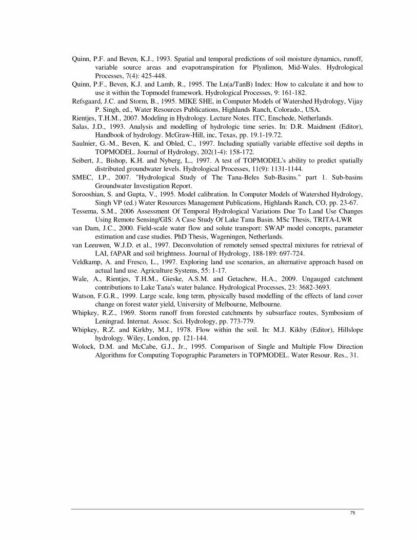
75
Quinn, P.F. and Beven, K.J., 1993. Spatial and temporal predictions of soil moisture dynamics, runoff,
variable source areas and evapotranspiration for Plynlimon, Mid-Wales. Hydrological
Processes, 7(4): 425-448.
Quinn, P.F., Beven, K.J. and Lamb, R., 1995. The Ln(a/TanB) Index: How to calculate it and how to
use it within the Topmodel framework. Hydrological Processes, 9: 161-182.
Refsgaard, J.C. and Storm, B., 1995. MIKE SHE, in Computer Models of Watershed Hydrology, Vijay
P. Singh, ed., Water Resources Publications, Highlands Ranch, Colorado., USA.
Rientjes, T.H.M., 2007. Modeling in Hydrology. Lecture Notes. ITC, Enschede, Netherlands.
Salas, J.D., 1993. Analysis and modelling of hydrologic time series. In: D.R. Maidment (Editor),
Handbook of hydrology. McGraw-Hill, inc, Texas, pp. 19.1-19.72.
Saulnier, G.-M., Beven, K. and Obled, C., 1997. Including spatially variable effective soil depths in
TOPMODEL. Journal of Hydrology, 202(1-4): 158-172.
Seibert, J., Bishop, K.H. and Nyberg, L., 1997. A test of TOPMODEL's ability to predict spatially
distributed groundwater levels. Hydrological Processes, 11(9): 1131-1144.
SMEC, I.P., 2007. "Hydrological Study of The Tana-Beles Sub-Basins." part 1. Sub-basins
Groundwater Investigation Report.
Sorooshian, S. and Gupta, V., 1995. Model calibration. In Computer Models of Watershed Hydrology,
Singh VP (ed.) Water Resources Management Publications, Highlands Ranch, CO, pp. 23-67.
Tessema, S.M., 2006 Assessment Of Temporal Hydrological Variations Due To Land Use Changes
Using Remote Sensing/GIS: A Case Study Of Lake Tana Basin. MSc Thesis, TRITA-LWR
van Dam, J.C., 2000. Field-scale water flow and solute transport: SWAP model concepts, parameter
estimation and case studies. PhD Thesis, Wageningen, Netherlands.
van Leeuwen, W.J.D. et al., 1997. Deconvolution of remotely sensed spectral mixtures for retrieval of
LAI, fAPAR and soil brightness. Journal of Hydrology, 188-189: 697-724.
Veldkamp, A. and Fresco, L., 1997. Exploring land use scenarios, an alternative approach based on
actual land use. Agriculture Systems, 55: 1-17.
Wale, A., Rientjes, T.H.M., Gieske, A.S.M. and Getachew, H.A., 2009. Ungauged catchment
contributions to Lake Tana's water balance. Hydrological Processes, 23: 3682-3693.
Watson, F.G.R., 1999. Large scale, long term, physically based modelling of the effects of land cover
change on forest water yield, University of Melbourne, Melbourne.
Whipkey, R.Z., 1969. Storm runoff from forested catchments by subsurface routes, Symbosium of
Leningrad. Internat. Assoc. Sci. Hydrology, pp. 773-779.
Whipkey, R.Z. and Kirkby, M.J., 1978. Flow within the soil. In: M.J. Kikby (Editor), Hillslope
hydrology. Wiley, London, pp. 121-144.
Wolock, D.M. and McCabe, G.J., Jr., 1995. Comparison of Single and Multiple Flow Direction
Algorithms for Computing Topographic Parameters in TOPMODEL. Water Resour. Res., 31.

76
APPENDICES
Appendix 1: acronyms and abbreviations
ASTER Advanced Space born Thermal Emission Radiometer
DEM Digital Elevation Model
DTM Digital Terrain Model
GIS Geographic Information System
GPS Global Positioning System
IDL Interactive Data Language
LAI Leaf Area Index
NASA National Aeronautics and Space Administration
RMSE Root Mean Square Error
RVE Relative Volume Error
SAVI Soil Adjusted Vegetation Index
UTM Universal Transverse Mercator
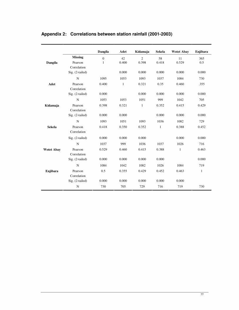
77
Appendix 2: Correlations between station rainfall (2001-2003)
Dangila Adet Kidamaja Sekela Wotet Abay Enjibara
Missing 0 42 2 58 11 365
Pearson
Correlation
1 0.400 0.398 0.418 0.529 0.5
Sig. (2-tailed) 0.000 0.000 0.000 0.000 0.000
Dangila
N 1095 1053 1093 1037 1084 730
Pearson
Correlation
0.400 1 0.321 0.35 0.460 .355
Sig. (2-tailed) 0.000 0.000 0.000 0.000 0.000
Adet
N 1053 1053 1051 999 1042 705
Pearson
Correlation
0.398 0.321 1 0.352 0.415 0.429
Sig. (2-tailed) 0.000 0.000 0.000 0.000 0.000
Kidamaja
N 1093 1051 1093 1036 1082 729
Pearson
Correlation
0.418 0.350 0.352 1 0.388 0.452
Sig. (2-tailed) 0.000 0.000 0.000 0.000 0.000
Sekela
N 1037 999 1036 1037 1026 716
Pearson
Correlation
0.529 0.460 0.415 0.388 1 0.463
Sig. (2-tailed) 0.000 0.000 0.000 0.000 0.000
Wotet Abay
N 1084 1042 1082 1026 1084 719
Pearson
Correlation
0.5 0.355 0.429 0.452 0.463 1
Sig. (2-tailed) 0.000 0.000 0.000 0.000 0.000
Enjibara
N 730 705 729 716 719 730
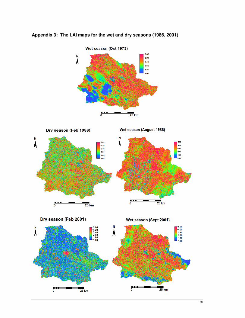
78
Appendix 3: The LAI maps for the wet and dry seasons (1986, 2001)
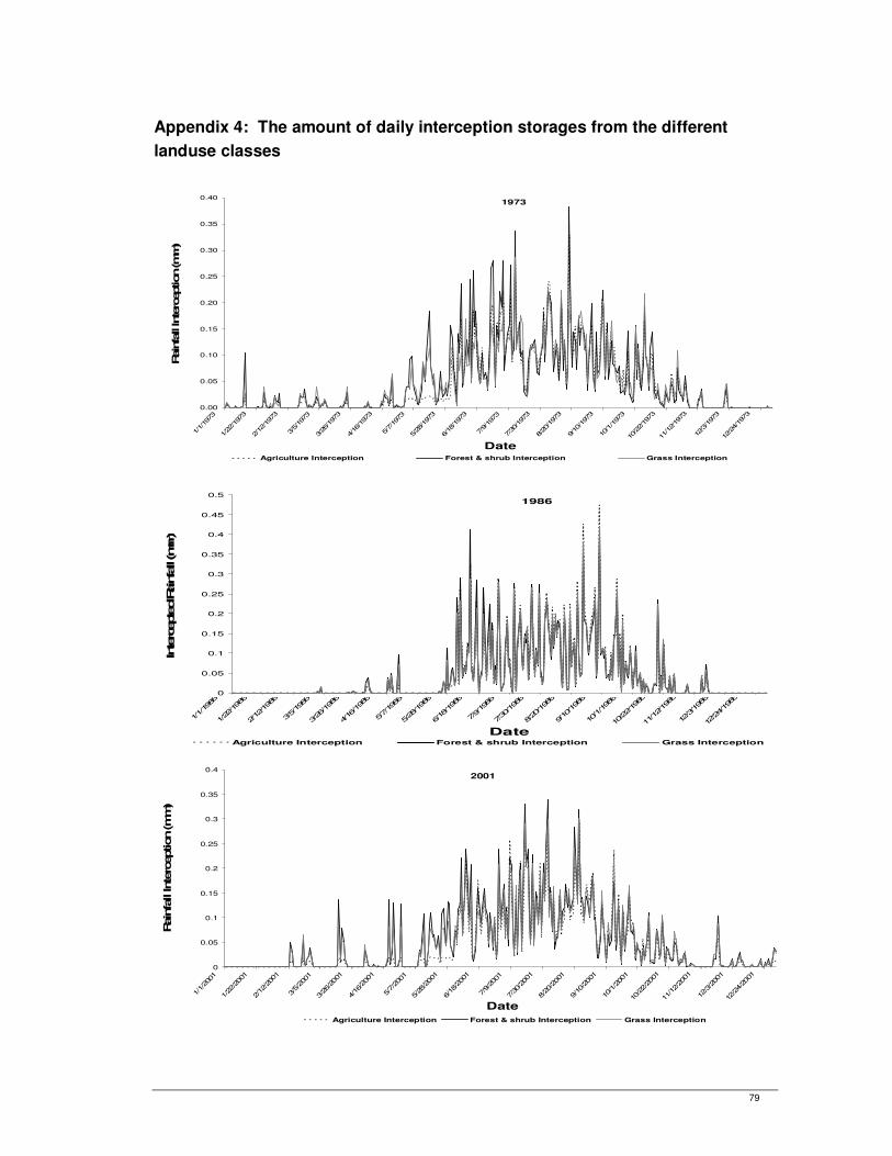
79
Appendix 4: The amount of daily interception storages from the different
landuse classes
0.00
0.05
0.10
0.15
0.20
0.25
0.30
0.35
0.40
1/1/19
73
1/22
/197
3
2/12
/197
3
3/5/19
73
3/26
/197
3
4/16
/197
3
5/7/19
73
5/28
/197
3
6/18
/197
3
7/9/19
73
7/30
/197
3
8/20
/197
3
9/10
/197
3
10/1/197
3
10/22/19
73
11/12/19
73
12/3/197
3
12/24/19
73
Date
Rain
fall Inte
rception (m
m)
Agriculture Interception Forest & shrub Interception Grass Interception
1973
1986
0
0.05
0.1
0.15
0.2
0.25
0.3
0.35
0.4
0.45
0.5
1/1/1986
1/22
/1986
2/12
/1986
3/5/1986
3/26
/1986
4/16
/1986
5/7/1986
5/28
/1986
6/18
/1986
7/9/1986
7/30
/1986
8/20
/1986
9/10
/1986
10/1/1986
10/22/1986
11/12/1986
12/3/1986
12/24/1986
Date
Intercepted R
ainfall (mm)
Agriculture Interception Forest & shrub Interception Grass Interception
2001
0
0.05
0.1
0.15
0.2
0.25
0.3
0.35
0.4
1/1/200
1
1/22/2001
2/12/2001
3/5/200
1
3/26/2001
4/16/2001
5/7/200
1
5/28/2001
6/18/2001
7/9/200
1
7/30/2001
8/20/2001
9/10/2001
10/1/2001
10/22/2001
11/12/2001
12/3/2001
12/24/2001
Date
Rain
fall Inte
rception (m
m)
Agriculture Interception Forest & shrub Interception Grass Interception