Hydrogel Drug Delivery:

Diffusion Models

Chun-Shu Wei, Chul Kim, Hyun-Je Kim, and Praopim Limsakul

BENG 221 – Fall 2012

2

Table of contents

Introduction……………………………………………………………………………...…..

Modeling Assumptions……………………………………………………………..….……

Drug diffusion in a swelling hydrogel……………………………………….……...

The initial and boundary conditions………………………………………….……..

Growing boundary…………………………………………………………….…….

Advection-diffusion equation and analytical solution…………………………………..…..

Landau transformation………………………………………………………….…...

Analytic solution of advection-diffusion equation………………………….………

Numerical Analysis………………………………………………………………………....

Parameter settings…………………………………………………………….……..

Analytical Solution…………………………………………………………….……

Finite Difference Method…………………………………………………………...

MATLAB pdepe………………………………………………………………….…

Comparison of Concentration Profiles in Different Types of Growth……………...

Conclusion and future work…………………………………………………………….…...

Reference………………………………………………………………………….………...

Appendix A: Analytical solution……………………………………………………….…...

Appendix B: Matlab Code………………………………………………………………......

3

4

4

5

5

7

7

8

9

9

9

10

11

12

13

14

15

19

3

Introduction

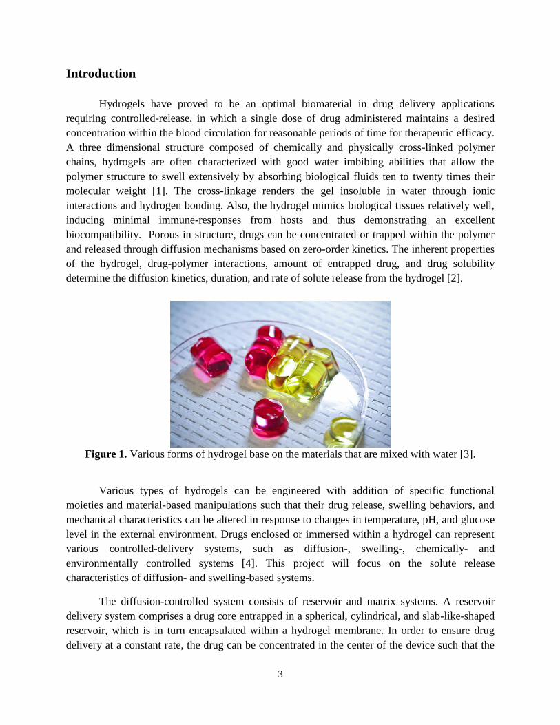
Hydrogels have proved to be an optimal biomaterial in drug delivery applications

requiring controlled-release, in which a single dose of drug administered maintains a desired

concentration within the blood circulation for reasonable periods of time for therapeutic efficacy.

A three dimensional structure composed of chemically and physically cross-linked polymer

chains, hydrogels are often characterized with good water imbibing abilities that allow the

polymer structure to swell extensively by absorbing biological fluids ten to twenty times their

molecular weight [1]. The cross-linkage renders the gel insoluble in water through ionic

interactions and hydrogen bonding. Also, the hydrogel mimics biological tissues relatively well,

inducing minimal immune-responses from hosts and thus demonstrating an excellent

biocompatibility. Porous in structure, drugs can be concentrated or trapped within the polymer

and released through diffusion mechanisms based on zero-order kinetics. The inherent properties

of the hydrogel, drug-polymer interactions, amount of entrapped drug, and drug solubility

determine the diffusion kinetics, duration, and rate of solute release from the hydrogel [2].

Figure 1. Various forms of hydrogel base on the materials that are mixed with water [3].

Various types of hydrogels can be engineered with addition of specific functional

moieties and material-based manipulations such that their drug release, swelling behaviors, and

mechanical characteristics can be altered in response to changes in temperature, pH, and glucose

level in the external environment. Drugs enclosed or immersed within a hydrogel can represent

various controlled-delivery systems, such as diffusion-, swelling-, chemically- and

environmentally controlled systems [4]. This project will focus on the solute release

characteristics of diffusion- and swelling-based systems.

The diffusion-controlled system consists of reservoir and matrix systems. A reservoir

delivery system comprises a drug core entrapped in a spherical, cylindrical, and slab-like-shaped

reservoir, which is in turn encapsulated within a hydrogel membrane. In order to ensure drug

delivery at a constant rate, the drug can be concentrated in the center of the device such that the

4

concentration gradient across the membrane is maintained zero. The matrix system features a

drug dispersed uniformly throughout the entire hydrogel lying within another bigger polymer

structure, rather than isolated and encapsulated within a separate reservoir in the center. These

hydrogel matrix tablets are constructed through compression of the drug and polymer powder

mixture. Drug permeates the macromolecular mesh or water filled pores into the exterior of the

hydrogel and blood stream. In case of swelling-controlled systems, the drug is initially dispersed

throughout the non-crystalline, glassy polymer containing the hydrogel. Upon contact with water

or some biofluid, the polymer starts to swell and its glass transition temperature is lowered such

that its brittle property is shifted towards assuming a more flexible, elastic property with

relaxation of molecular chains, which then allows for drug diffusion out of the rubbery boundary

of the polymer. In many cases, a combination of both diffusion and swelling-mediated drug

releases occurs [5].

Modeling Assumptions

Drug diffusion in a swelling hydrogel

Let the drug concentration within the polymer equal , , ,c c x y z t , at any time in three

dimensional domains. The drug can diffuse out of the domains at the boundaries which may

swell or grow as fluids are absorbed. The general advection-diffusion equation for a growing

domain [6] is

2cD c c

t

u . ( 1)

We consider drug diffusing out of the domain in only one dimension, so the velocity of drug is

uu i , and the diffusion equation will be

2

2

c c u cD c u

t x x x

where 2

2

c cD

t x

: homogeneous diffusion equation

u

cx

: the hydrogel is swollen, so the local volume change

cu

x

: the local concentration dilutes.

5

The initial and boundary conditions

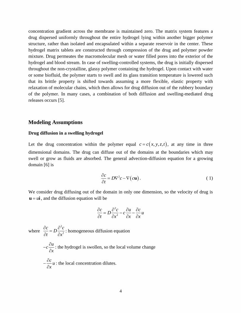
In the beginning, the drug concentration is assumed to be constant everywhere inside the

hydrogel with dimension, 0 < x < X(0). For t > 0, hydrogel is swollen with the outside fluid. Its

boundary will grow at one side x = X(t) = Lf(t), where L is the original length of hydrogel, and

f(t) is a growing function over time (f(t) > 1). In this boundary, the concentration is assumed to

be zero all the time. We can express the problem with its initial and boundary conditions as:

2

2

c c c uD u c

t x x x

, 0 ( ), t > 0x X t ( 2)

with

( ,0) 1 ,0 0

(0)

0, 0 ,t > 0

, 0

c x x X

X L

ct

x

c X t t

( 3)

Figure 2. The mixed solution between hydrogel and drug is surrounded by bio-fluid. Left figure

shows hydrogel system at t=0. Right figure shows the system when t > 0, on the right edge of

hydrogel growing as a function of time.

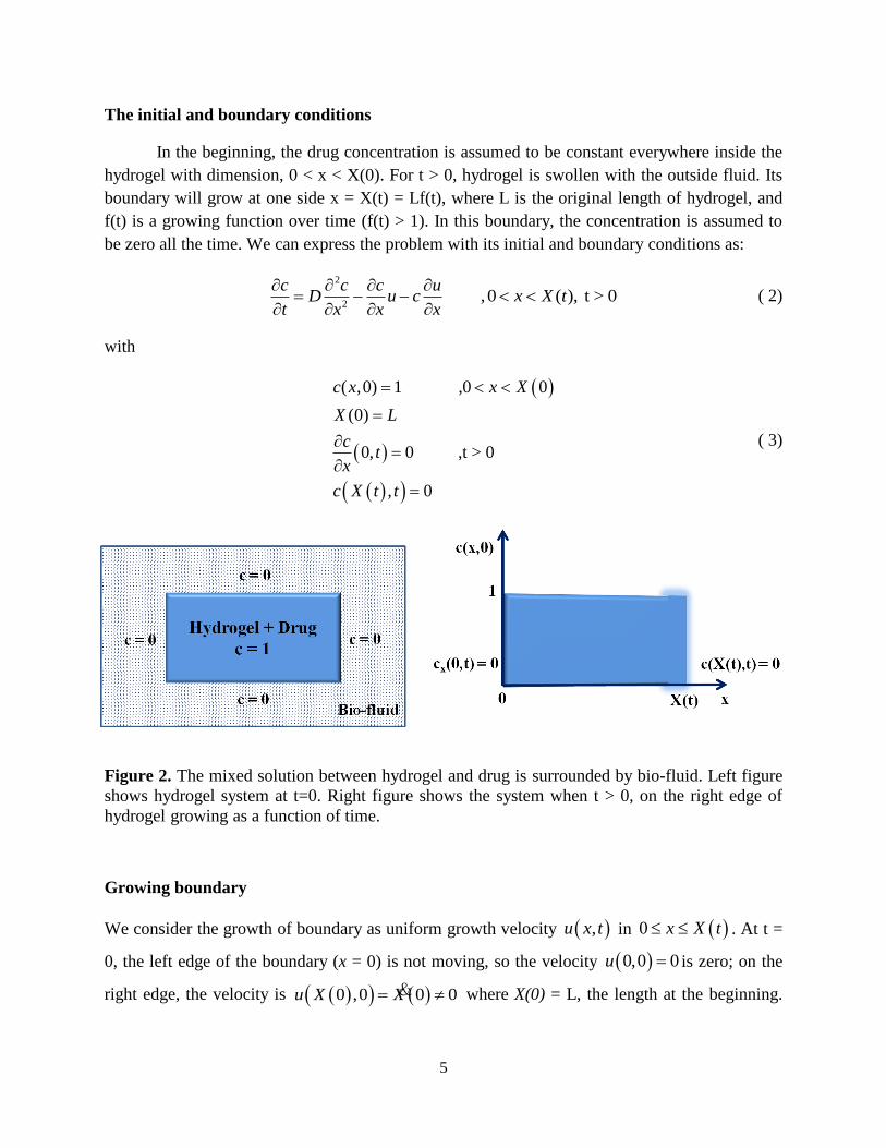
Growing boundary

We consider the growth of boundary as uniform growth velocity ,u x t in 0 x X t . At t =

0, the left edge of the boundary (x = 0) is not moving, so the velocity 0,0 0u is zero; on the

right edge, the velocity is 0 ,0 0 0u X X & where X(0) = L, the length at the beginning.

6

At time t > 0, the velocity of the left edge is still the same 0, 0u t ; on the right edge, the

boundary grows over time. Since X(t) is the growing length of hydrogel on the right edge, the

growing velocity of the edge can be written as

,dX t

u X t t X tdt

& . From this relation

between the growing edge velocity and length, the gradient of velocity can be rewritten in terms

of moving length as shown below.

0

, 0,

X tdX tu

u X t t u t dxx dt

If velocity gradient is independent of x,

0

X tu u

dx X t X t X tx x

& & ,

therefore the velocity as a function of X(t) is

,

X t X tuu x t x

x X t X t

& &. ( 4)

Now, the growing edge velocity can be written in terms of growing edge length as shown in

Equation (4). We can correlate the growth of the system with the function X(t) (see [7]). In this

work, we study two types of growth function.

1. The growth function increases over time. In this case, the domain expands to infinite

volume as time increase such that

- Linear growth

1X t L rt ( 5)

- Exponential growth

rtX t Le ( 6)

2. The growth function increases up to a finite volume and remains the same size as

time increase i.e.

- Logistic growth

1 1/ 1

rt

rt

LeX t

m e

( 7)

7

Figure 3. Growth function: linear, exponential, and logistic growth [5].

Advection-diffusion equation and analytical solution

The advection-diffusion equation in Equation (2) can be rewritten by substituting the expression

defined in Equation (4) as

2

2

c c X c XD x c

t x X x X

& & in 0 ( ), t > 0x X t ( 8)

with the initial and boundary conditions:

( ,0) 1 ,0 0

(0)

0, 0 ,t > 0

, 0

c x x X

X L

ct

x

c X t t

( 9)

Landau transformation

Two difficulties with analytically solving Equation (8) are the presence of an advection term,

X cx

X x

&, and the moving boundary of hydrogel, X(t), whose behavior is described by

Equations (5)-(7). With these difficulties, Landau transformation [8] is used to simplify the

problem. This transformation is defined by

x

X t , and t . ( 10)

8

If any phase extends from x = 0 to x = X(t), then ζ in the above form is used to fix the extent of

that phase to the new domain 0 ≤ ζ ≤ 1.

Therefore the new diffusion equation becomes easier to solve analytically (see Appendix A)

2

2 2

c D c X c

X X

& in 0 1, 0 ( 11)

with the new initial and boundary conditions:

( ,0) 1 ,0 1

0, 0 , > 0

1, 0

c

c

x

c

( 12)

Analytic solution of advection-diffusion equation

The concentration of drug released from the swelling hydrogel can be defined as a function of

Landau variables by using the technique of variable separation (see Appendix A):

2

2

0

2 1

2

0

14 2 1, cos

2 1 2

t

nnD X dt

n

L nc e

n X

( 13)

This solution is a drug concentration in terms of Landau variables ξ and τ. It can be transformed

back to the original variables by using the relations in Equation (10), so the solution of this

problem is:

22

0

2 1

2

0

1 2 14, cos

2 1 2

t

t

nnD X t dt

n

n xLc x t e

n X t X t

( 14)

The above solution can be used to explain how drug concentration changes with respect to time

and spatial variation in one dimension, as the drug is released from the hydrogel expanding with

a moving boundary. This expansion can be described by the function X(t), based on three

different growth models: linear, exponential , and logistic growth (Equations (5)-(7)).

9

Numerical Analysis

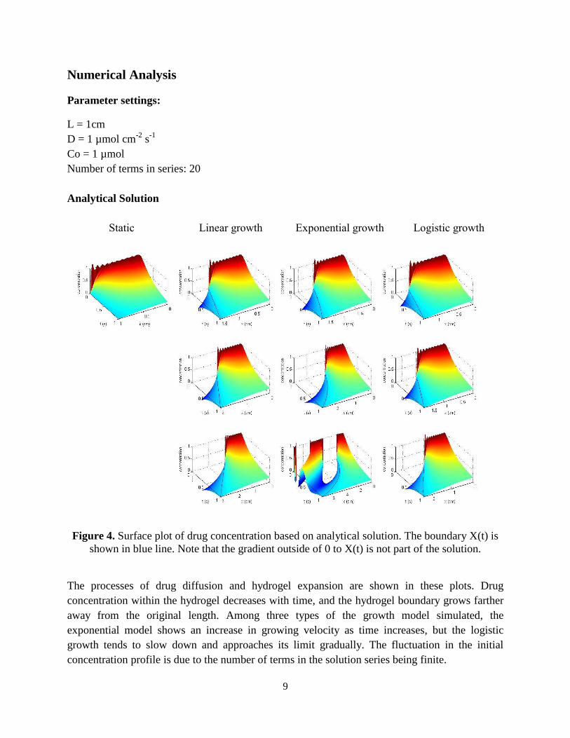
Parameter settings:

L = 1cm

D = 1 µmol cm-2

s-1

Co = 1 µmol

Number of terms in series: 20

Analytical Solution

Static Linear growth Exponential growth Logistic growth

Figure 4. Surface plot of drug concentration based on analytical solution. The boundary X(t) is

shown in blue line. Note that the gradient outside of 0 to X(t) is not part of the solution.

The processes of drug diffusion and hydrogel expansion are shown in these plots. Drug

concentration within the hydrogel decreases with time, and the hydrogel boundary grows farther

away from the original length. Among three types of the growth model simulated, the

exponential model shows an increase in growing velocity as time increases, but the logistic

growth tends to slow down and approaches its limit gradually. The fluctuation in the initial

concentration profile is due to the number of terms in the solution series being finite.

10

Finite Difference Method

Static Linear growth Exponential growth Logistic growth

Figure 5. Surface plot of drug concentration using finite difference method.

11

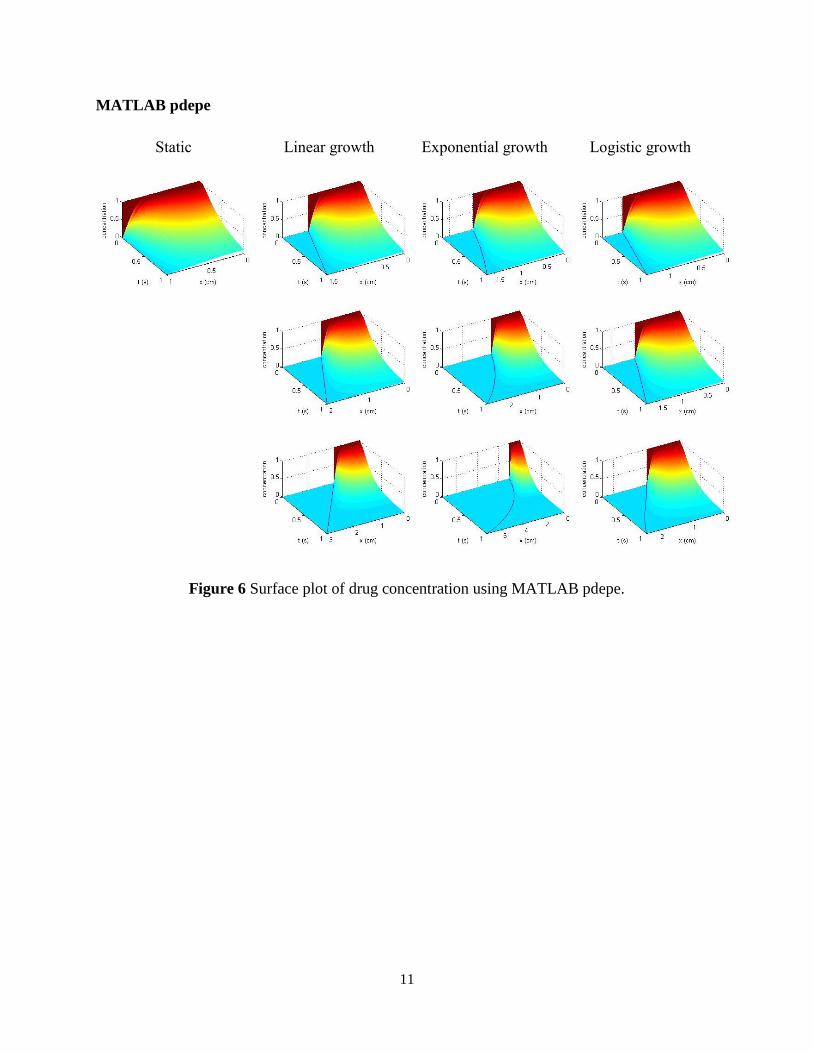
MATLAB pdepe

Static Linear growth Exponential growth Logistic growth

Figure 6 Surface plot of drug concentration using MATLAB pdepe.

12

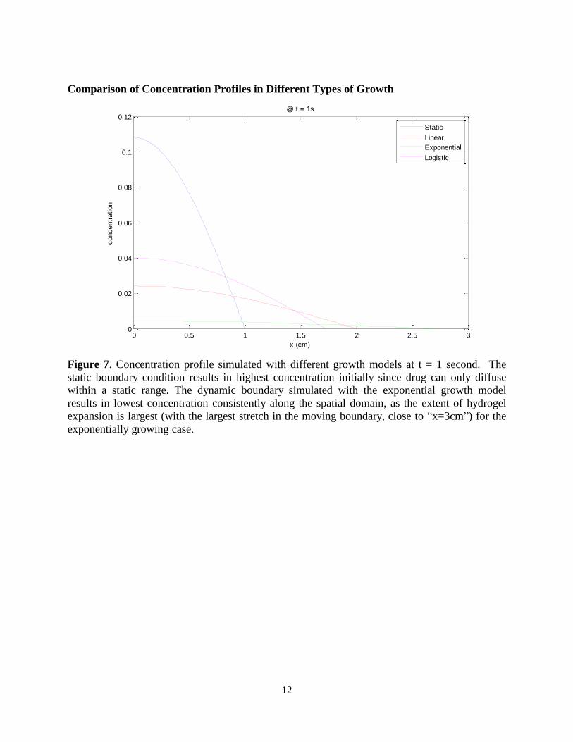
Comparison of Concentration Profiles in Different Types of Growth

Figure 7. Concentration profile simulated with different growth models at t = 1 second. The

static boundary condition results in highest concentration initially since drug can only diffuse

within a static range. The dynamic boundary simulated with the exponential growth model

results in lowest concentration consistently along the spatial domain, as the extent of hydrogel

expansion is largest (with the largest stretch in the moving boundary, close to “x=3cm”) for the

exponentially growing case.

0 0.5 1 1.5 2 2.5 30

0.02

0.04

0.06

0.08

0.1

0.12

x (cm)

concentr

ation

@ t = 1s

Static

Linear

Exponential

Logistic

13

Conclusion and Future work

Limitation and future work

The hydrogel swelling should be technically modeled with respect to all three dimensions

to approximate its behavior in reality most accurately, even though the growth models presented

in this report are sufficient enough to demonstrate how much the hydrogel swells one

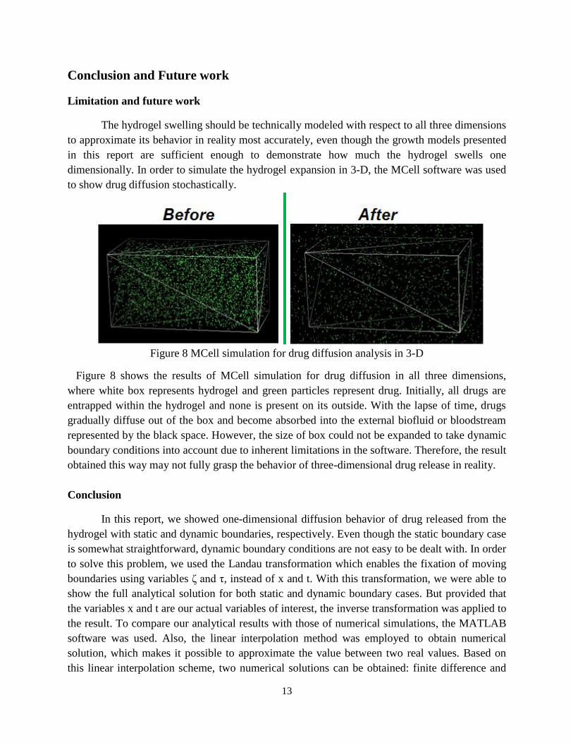
dimensionally. In order to simulate the hydrogel expansion in 3-D, the MCell software was used

to show drug diffusion stochastically.

Figure 8 MCell simulation for drug diffusion analysis in 3-D

Figure 8 shows the results of MCell simulation for drug diffusion in all three dimensions,

where white box represents hydrogel and green particles represent drug. Initially, all drugs are

entrapped within the hydrogel and none is present on its outside. With the lapse of time, drugs

gradually diffuse out of the box and become absorbed into the external biofluid or bloodstream

represented by the black space. However, the size of box could not be expanded to take dynamic

boundary conditions into account due to inherent limitations in the software. Therefore, the result

obtained this way may not fully grasp the behavior of three-dimensional drug release in reality.

Conclusion

In this report, we showed one-dimensional diffusion behavior of drug released from the

hydrogel with static and dynamic boundaries, respectively. Even though the static boundary case

is somewhat straightforward, dynamic boundary conditions are not easy to be dealt with. In order

to solve this problem, we used the Landau transformation which enables the fixation of moving

boundaries using variables ζ and τ, instead of x and t. With this transformation, we were able to

show the full analytical solution for both static and dynamic boundary cases. But provided that

the variables x and t are our actual variables of interest, the inverse transformation was applied to

the result. To compare our analytical results with those of numerical simulations, the MATLAB

software was used. Also, the linear interpolation method was employed to obtain numerical

solution, which makes it possible to approximate the value between two real values. Based on

this linear interpolation scheme, two numerical solutions can be obtained: finite difference and

14

pdepde. These results are highly similar to those of our analytical solution, with some minor

inevitable discrepancies that can be adequately explained. Finally, the MCell simulation results

were shown that approximate three dimensional diffusion of drug from the hydrogel with the

static boundary conditions only.

References

[1] Amin, Saima, Saeid Rajabnezhad, and Kanchan Cohli. "Hydrogels as Potential Drug

Delivery Systems." Scientific Research and Essay 3.11 (2009): 1175-183. Academic

Journals, Nov. 2009. Web. 23 Nov. 2012.

<http://www.academicjournals.org/sre/pdf/pdf2009/nov/Amin%20et%20al.pdf>.

[2] Kim, S. W., Y. H. Bae, and T. Okano. "Hydrogels: Swelling, Drug Loading, and

Release." NCBI 90th ser. 3.283 (1992): n. pag. PubMed. US National Library of

Medicine National Institutes of Health, 9 Mar. 1992. Web. 23 Nov. 2012.

<http://www.ncbi.nlm.nih.gov/pubmed/1614957>.

[3] M. Fellet. Organic hydrogel outperforms typical carbon supercapacitors. Available at:

URL: http://arstechnica.com/science/2012/06/organic-hydrogel-outperforms-typical-

carbon-supercapacitors/. Accessed Nov 21, 2012.

[4] F. Bierbrauer, Hydrogel Drug Delivery: Diffusion models, School of Mathematics and

Applied Statistics, University of Wollongong, Australia.

[5] Lowman, Anthony M., and Nikolaos A. Peppas. "Hydrogels." Encyclopedia of

Controlled Drug Delivery 1 (1999): 397-418. PubMed. Wiley: New York. Web. 23 Nov.

2012

[6] I. Rubinstein, L. Rubinstein, Partial Differential Equations in Classical Mathematical

Physics, CUP, Cambridge, 1993.

[7] V. Alexiades, A.D. Solomon, Mathematical Modeling of Melting and Freezing Processes,

Hemisphere Publishing, Washington, 1993.

[8] K.A. Landman, G.J. Pettet, D.F. Newgreen, Mathematical Models of Cell Colonisation of

Uniformly Growing Domains, PNAS B. Math. Biol., 65 (2003), 235-262.

15

Appendix A: Analytical solution

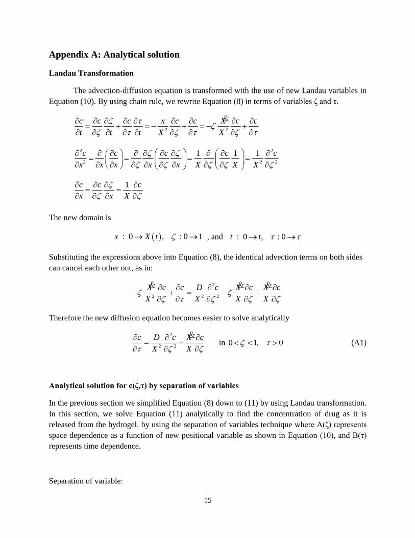
Landau Transformation

The advection-diffusion equation is transformed with the use of new Landau variables in

Equation (10). By using chain rule, we rewrite Equation (8) in terms of variables ζ and τ.

2 2

c c c x c c X c c

t t t X X

&

2 2

2 2 2

1 1 1c c c c c

x x x x x X X X

1c c c

x x X

The new domain is

: 0 , : 0 1x X t , and : 0 , : 0t t

Substituting the expressions above into Equation (8), the identical advection terms on both sides

can cancel each other out, as in:

2

2 2 2

X c c D c X c X c

X X X X

& & &

Therefore the new diffusion equation becomes easier to solve analytically

2

2 2

c D c X c

X X

& in 0 1, 0 (A1)

Analytical solution for c(ζ,τ) by separation of variables

In the previous section we simplified Equation (8) down to (11) by using Landau transformation.

In this section, we solve Equation (11) analytically to find the concentration of drug as it is

released from the hydrogel, by using the separation of variables technique where A(ζ) represents

space dependence as a function of new positional variable as shown in Equation (10), and B(τ)

represents time dependence.

Separation of variable:

16

,c A B (A2)

Substituting it into Equation (11):

2

2 2

1B A dXDA B A B

X dX

.

Using the abbreviated form, the above equation can be reduced to:

2

D XAB BA AB

X X &

&

Dividing both sides by AB:

2

B D A X

B X A X

& &

Rearranging to get all time dependent functions on the left and space dependent functions on the

right-hand side, the expressions on both sides equal a negative constant:

22X B XX A

D B D A

& &

The partial differential equation in (11) can then be reduced into two ordinary differential

equations:

22

20 ,and 0

X DB B A A

X X

&&

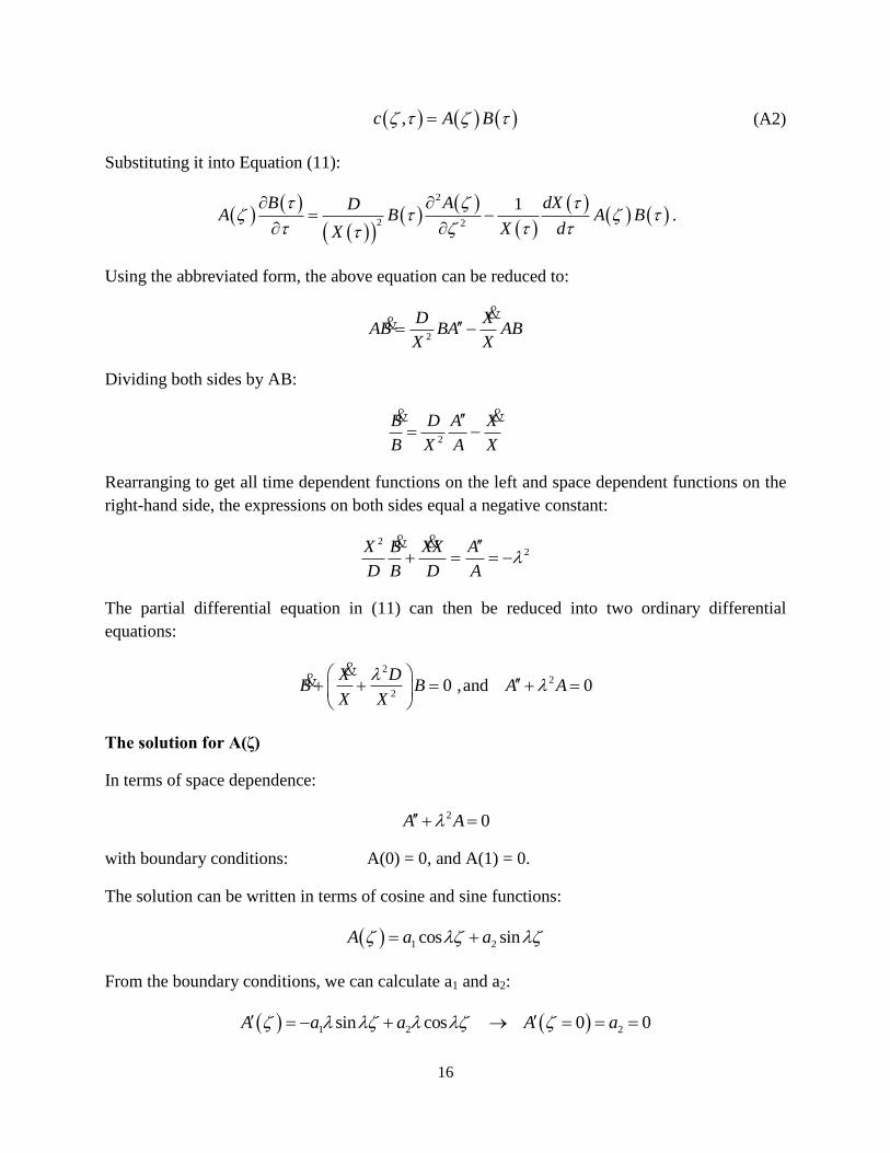
The solution for A(ζ)

In terms of space dependence:

2 0A A

with boundary conditions: A(0) = 0, and A(1) = 0.

The solution can be written in terms of cosine and sine functions:

1 2cos sinA a a

From the boundary conditions, we can calculate a1 and a2:

1 2 2sin cos 0 0A a a A a

17

1 2 1cos sin 1 cos 0A a a A a

In order to avoid obtaining a trivial solution, the coefficient a2 cannot be made to equal zero but

rather cosλ is set equal to zero such that

1 2 1 = , 0,1,2,...

2 2

nn n

.

Therefore, the solution for A is:

2 1

cos , n = 0,1,2,...2

n n

nA a

. (A3)

The solution for B(τ)

In terms of time dependence:

2

20

X DB B

X X

&&

Since this is the first order ODE, we can find the solution B(τ) by simple integration. In order to

do so, we have to rearrange the equation by separating B from time dependence terms:

2

2

1 X DB

B X X

&&

Integration with respect to B and τ yields:

2

20 0

1B

B t

X DdB dt

B X X

&

Rearranging the terms and solving the integral:

2

20 0

1B

B t

X DdB dt

B X X

&

2

20 0

1ln ln

t t

dX DB dt dt C

X dt X

2 2

0ln ln ln 0 ln

tB X X D X dt C

18

2 2

0ln

t

B XD X dt

CL

The solution becomes:

2 2

0tD X dtCL

B eX

(A4)

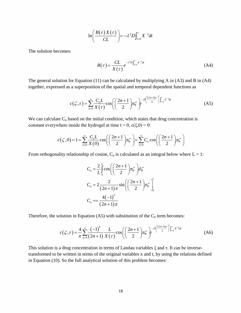
The general solution for Equation (11) can be calculated by multiplying A in (A3) and B in (A4)

together, expressed as a superposition of the spatial and temporal dependent functions as

2

2

0

2 1

2

0

2 1, cos

2

t

nD X dt

n

n

C L nc e

X

(A5)

We can calculate Cn based on the initial condition, which states that drug concentration is

constant everywhere inside the hydrogel at time t = 0, c(ξ,0) = 0:

0 0

2 1 2 1,0 1 cos cos

0 2 2

nn

n n

C L n nc C

X

From orthogonality relationship of cosine, Cn is calculated as an integral below where L = 1:

0

1

0

2 2 1cos

2

2 2 12 sin

2 1 2

4 1

2 1

L

n

n

n

n

nC d

L

nC

n

Cn

Therefore, the solution in Equation (A5) with substitution of the Cn term becomes:

2

2

0

2 1

2

0

14 2 1, cos

2 1 2

t

nnD X dt

n

L nc e

n X

(A6)

This solution is a drug concentration in terms of Landau variables ξ and τ. It can be inverse-

transformed to be written in terms of the original variables x and t, by using the relations defined

in Equation (10). So the full analytical solution of this problem becomes:

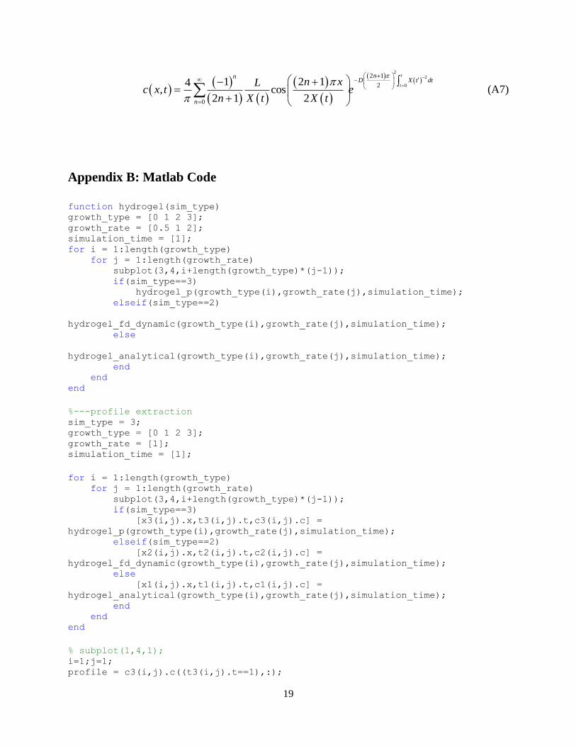
19

22

0

2 1

2

0

1 2 14, cos

2 1 2

t

t

nnD X t dt

n

n xLc x t e

n X t X t

(A7)

Appendix B: Matlab Code

function hydrogel(sim_type) growth_type = [0 1 2 3]; growth_rate = [0.5 1 2]; simulation_time = [1]; for i = 1:length(growth_type) for j = 1:length(growth_rate) subplot(3,4,i+length(growth_type)*(j-1)); if(sim_type==3) hydrogel_p(growth_type(i),growth_rate(j),simulation_time); elseif(sim_type==2)

hydrogel_fd_dynamic(growth_type(i),growth_rate(j),simulation_time); else

hydrogel_analytical(growth_type(i),growth_rate(j),simulation_time); end end end

%---profile extraction sim_type = 3; growth_type = [0 1 2 3]; growth_rate = [1]; simulation_time = [1];

for i = 1:length(growth_type) for j = 1:length(growth_rate) subplot(3,4,i+length(growth_type)*(j-1)); if(sim_type==3) [x3(i,j).x,t3(i,j).t,c3(i,j).c] =

hydrogel_p(growth_type(i),growth_rate(j),simulation_time); elseif(sim_type==2) [x2(i,j).x,t2(i,j).t,c2(i,j).c] =

hydrogel_fd_dynamic(growth_type(i),growth_rate(j),simulation_time); else [x1(i,j).x,t1(i,j).t,c1(i,j).c] =

hydrogel_analytical(growth_type(i),growth_rate(j),simulation_time); end end end

% subplot(1,4,1); i=1;j=1; profile = c3(i,j).c((t3(i,j).t==1),:);

20

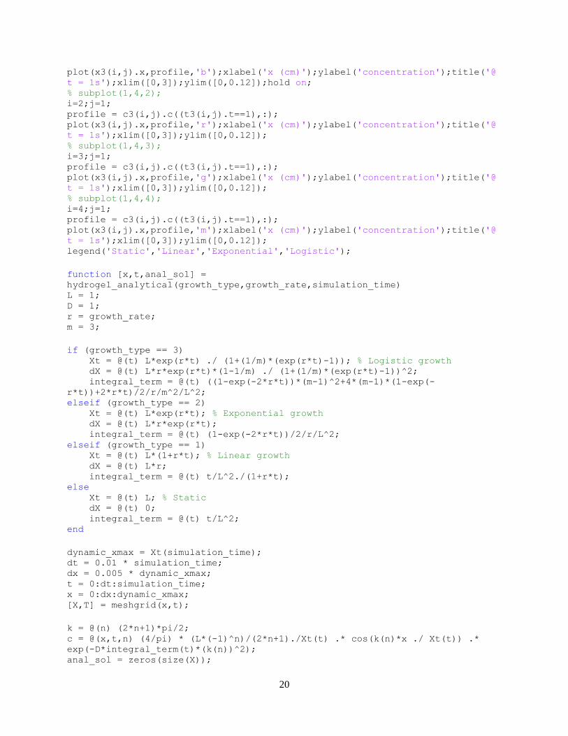
plot(x3(i,j).x,profile,'b');xlabel('x (cm)');ylabel('concentration');title('@

t = 1s');xlim([0,3]);ylim([0,0.12]);hold on; % subplot(1,4,2); i=2;j=1; profile = c3(i,j).c((t3(i,j).t==1),:); plot(x3(i,j).x,profile,'r');xlabel('x (cm)');ylabel('concentration');title('@

t = 1s');xlim([0,3]);ylim([0,0.12]); % subplot(1,4,3); i=3;j=1; profile = c3(i,j).c((t3(i,j).t==1),:); plot(x3(i,j).x,profile,'g');xlabel('x (cm)');ylabel('concentration');title('@

t = 1s');xlim([0,3]);ylim([0,0.12]); % subplot(1,4,4); i=4;j=1; profile = c3(i,j).c((t3(i,j).t==1),:); plot(x3(i,j).x,profile,'m');xlabel('x (cm)');ylabel('concentration');title('@

t = 1s');xlim([0,3]);ylim([0,0.12]); legend('Static','Linear','Exponential','Logistic');

function [x,t,anal_sol] =

hydrogel_analytical(growth_type,growth_rate,simulation_time) L = 1; D = 1; r = growth_rate; m = 3;

if (growth_type == 3) Xt = @(t) L*exp(r*t) ./ (1+(1/m)*(exp(r*t)-1)); % Logistic growth dX = @(t) L*r*exp(r*t)*(1-1/m) ./ (1+(1/m)*(exp(r*t)-1))^2; integral_term = @(t) ((1-exp(-2*r*t))*(m-1)^2+4*(m-1)*(1-exp(-

r*t))+2*r*t)/2/r/m^2/L^2; elseif (growth_type == 2) Xt = @(t) L*exp(r*t); % Exponential growth dX = @(t) L*r*exp(r*t); integral_term = @(t) (1-exp(-2*r*t))/2/r/L^2; elseif (growth_type == 1) Xt = @(t) L*(1+r*t); % Linear growth dX = @(t) L*r; integral_term = @(t) t/L^2./(1+r*t); else Xt = @(t) L; % Static dX = @(t) 0; integral_term = @(t) t/L^2; end

dynamic_xmax = Xt(simulation_time); dt = 0.01 * simulation_time; dx = 0.005 * dynamic_xmax; t = 0:dt:simulation_time; x = 0:dx:dynamic_xmax; [X,T] = meshgrid(x,t);

k = @(n) (2*n+1)*pi/2; c = @(x,t,n) (4/pi) * (L*(-1)^n)/(2*n+1)./Xt(t) .* cos(k(n)*x ./ Xt(t)) .*

exp(-D*integral_term(t)*(k(n))^2); anal_sol = zeros(size(X));

21

for i = 1:20 n = i-1; anal_sol = anal_sol + c(X,T,n); end

surf(x,t,anal_sol,'LineStyle','none');hold on; line(Xt(t),t,'Color','b'); xlabel('x (cm)');xlim([0 dynamic_xmax]); ylabel('t (s)');ylim([0 simulation_time]); zlabel('concentration');zlim([0 1]); view(150,50); caxis([-0.5 1]);

function [dynamic_x,tmesh,fd_dynamic] =

hydrogel_fd_dynamic(growth_type,growth_rate,simulation_time)

L = 1; D = 1; r = growth_rate; m = 3;

simulation_x = L; dt = 0.00025 * simulation_time; dx = 0.025 * simulation_x; tmesh = 0:dt:simulation_time; xmesh = 0:dx:simulation_x; nx = length(xmesh); nt = length(tmesh); sol_fd = zeros(nt,nx); sol_fd(1,:) = ones(1,nx); sol_fd(:,nx) = 0; update_const = D*dt/dx^2; for t = 1:nt-1 for x = 1 sol_fd(t+1,1) = sol_fd(t,2); end for x = 2:nx-1 sol_fd(t+1,x) = sol_fd(t,x) + ... update_const*(sol_fd(t,x+1)+sol_fd(t,x-1)-2*sol_fd(t,x)) -... (r*dt/(1+r*t))*(sol_fd(t,x)+(x/2/dx)*(sol_fd(t,x+1)-sol_fd(t,x-

1))); end end

if (growth_type == 3) Xt = @(t) L*exp(r*t) ./ (1+(1/m)*(exp(r*t)-1)); % Logistic growth dX = @(t) L*r*exp(r*t)*(1-1/m) ./ (1+(1/m)*(exp(r*t)-1))^2; elseif (growth_type == 2) Xt = @(t) L*exp(r*t); % Exponential growth dX = @(t) L*r*exp(r*t); elseif (growth_type == 1) Xt = @(t) L*(1+r*t); % Linear growth dX = @(t) L*r; else Xt = @(t) L; % Static dX = @(t) 0;

22

end dynamic_xmax = Xt(simulation_time); dynamic_x = 0:dx:dynamic_xmax; fd_dynamic = zeros(length(tmesh),length(dynamic_x)); for j = 1:length(tmesh); interp_t = tmesh(j); x_max = Xt(interp_t); interp_x = linspace(0,simulation_x,floor(x_max/dx)+1); interp_sol = interp1(xmesh,sol_fd(j,:),interp_x); fd_dynamic(j,1:length(interp_sol)) = interp_sol; clear interp_sol; end

surf(dynamic_x,tmesh,fd_dynamic,'LineStyle','none');hold on; line(Xt(tmesh),tmesh,'Color','b'); xlabel('x (cm)');xlim([0 dynamic_xmax]); ylabel('t (s)');ylim([0 simulation_time]); zlabel('concentration');zlim([0 1]); view(150,50); caxis([-0.5 1]);

function [dynamic_x,t,pde_dynamic] =

hydrogel_p(gt,growth_rate,simulation_time) global L D r m growth_type; L = 1; D = 1; r = growth_rate; m = 3; growth_type = gt; simulation_x = L; dt = 0.01 * simulation_time; dx = 0.005 * simulation_x; t = 0:dt:simulation_time; x = 0:dx:simulation_x;

if (growth_type == 3) Xt = @(t) L*exp(r*t) ./ (1+(1/m)*(exp(r*t)-1)); % Logistic growth dX = @(t) L*r*exp(r*t)*(1-1/m) ./ (1+(1/m)*(exp(r*t)-1))^2; elseif (growth_type == 2) Xt = @(t) L*exp(r*t); % Exponential growth dX = @(t) L*r*exp(r*t); elseif (growth_type == 1) Xt = @(t) L*(1+r*t); % Linear growth dX = @(t) L*r; else Xt = @(t) L; % Static dX = @(t) 0; end

pde_sol = pdepe(0,@hydrogel_pde,@hydrogel_ic,@hydrogel_bc,x,t); dynamic_xmax = Xt(simulation_time); dynamic_x = 0:dx:dynamic_xmax; pde_dynamic = zeros(size(pde_sol,1),length(dynamic_x));

for j = 1:length(t); interp_t = t(j);

23

x_max = Xt(interp_t); interp_x = linspace(0,simulation_x,floor(x_max/dx)+1); interp_sol = interp1(x,pde_sol(j,:),interp_x); pde_dynamic(j,1:length(interp_sol)) = interp_sol; clear interp_sol; end surf(dynamic_x,t,pde_dynamic,'LineStyle','none');hold on; line(Xt(t),t,'Color','b'); xlabel('x (cm)');xlim([0 dynamic_xmax]); ylabel('t (s)');ylim([0 simulation_time]); zlabel('concentration');zlim([0 1]); view(150,50); caxis([-0.5 1]);

%------------------------------- function [c,f,s] = hydrogel_pde(x,t,u,DuDx) global L D r m growth_type; if (growth_type == 3) Xt = @(t) L*exp(r*t) ./ (1+(1/m)*(exp(r*t)-1)); % Logistic growth dX = @(t) L*r*exp(r*t)*(1-1/m) ./ (1+(1/m)*(exp(r*t)-1))^2; elseif (growth_type == 2) Xt = @(t) L*exp(r*t); % Exponential growth dX = @(t) L*r*exp(r*t); elseif (growth_type == 1) Xt = @(t) L*(1+r*t); % Linear growth dX = @(t) L*r; else Xt = @(t) L; % Static dX = @(t) 0; end c = L^2/D; f = DuDx; s = -(dX(t).*Xt(t)/D)*u; function u0 = hydrogel_ic(x) % Initial conditions function u0 = 1; function [pl, ql, pr, qr] = hydrogel_bc(xl, ul, xr, ur, t) % Boundary conditions function pl = 0; % no value left boundary condition ql = 1; % zero flux left boundary condition pr = ur; % zero value right boundary condition qr = 0; % no flux right boundary condition