Embed Size (px)
Citation preview

Hydroelectric Power Generation and Distribution Planning Under
Supply Uncertainty
by
Govind R. Joshi
A Thesis
Submitted to
The Department of Engineering
Colorado State University-Pueblo
In partial fulfillment of requirements for the degree of
Master of Science
Completed on December 16th, 2016

ii
ABSTRACT
Govind Raj Joshi for the degree of Master of Science in Industrial and Systems Engineering
presented on December 16th, 2016.
Hydroelectric Power Generation and Distribution Planning Under Supply Uncertainty
Abstract approved: -------------------------------------------
Ebisa D. Wollega, Ph.D.
Hydroelectric power system is a renewable energy type that generates electrical energy
from water flow. An integrated hydroelectric power system may consist of water storage dams and
run-of-river (ROR) hydroelectric power projects. Storage dams store water and regulate water flow
so that power from the storage projects dispatch can follow a pre-planned schedule. Power supply
from ROR projects is uncertain because water flow in the river, and hence power production
capacity, is largely determined by uncertain weather factors. Hydroelectric generator dispatch
problem has been widely studied in the literature; however, very little work is available to address
the dispatch and distribution planning of an integrated ROR and storage hydroelectric projects.
This thesis combines both ROR projects and storage dam projects and formulate the problem as a
stochastic program to minimize the cost of energy generation and distribution under ROR projects
supply uncertainty. Input data from the Integrated Nepal Power System are used to solve the
problem and run experiments. Numerical comparisons of stochastic solution (SS), expected value
(EEV), and wait and see (W&S) solutions are made. These solution approaches give economic
dispatch of generators and optimal distribution plan that the power system operators (PSO) can
use to coordinate, control, and monitor the power generation and distribution system. The W&S
solution approach provided the least cost plan. The EEV solution was worse than the SS. The PSO
may invest in advanced technologies to more accurately reveal the uncertainties in the planning
process, to operate at the W&S operational cost. However, the tradeoff between using the SS
solution and investing in new technologies to operate at W&S solution may require rigorous
feasibility study.

iii
Certificate of Acceptance
This thesis presented in partial fulfillment of the requirements for the degree of
Master of Science
has been accepted by the program of Industrial and Systems Engineering,
Colorado State University - Pueblo
APPROVED
---------------------------------------------------------------------------------------------------------------------
Dr. Ebisa D. Wollega Date
Assistant Professor of Engineering and Committee Chair
---------------------------------------------------------------------------------------------------------------------
Dr. Leonardo Bedoya-Valencia Date
Associate Professor of Engineering and Committee Member
---------------------------------------------------------------------------------------------------------------------
Dr. Jane M. Fraser Date
Professor and Director of Engineering and Committee Member
Master’s Candidate Govind R. Joshi
Date of thesis presentation December 16, 2016

iv
ACKNOWLEDGEMENTS
This thesis would not have been possible without the guidance and the help of several
individuals who contributed and extended their valuable assistance in the preparation and
completion of this research.
First and foremost, I offer my utmost gratitude to my academic advisor and committee
chair, Dr. Ebisa Wollega, for his support throughout the development of this thesis with his
knowledge and patience. I also would like to thank the Department of Engineering at Colorado
State University -Pueblo for giving me the opportunity to work on this thesis and for providing me
the required resources to carry out this research.
Last but not the least, I would like to thank my parents as well as my uncle Rajendra
Awasthi and aunt Kacie Awasthi for their guidance and support throughout my master degree at
Colorado State University - Pueblo.

v
ABBREVIATIONS
Table I List of abbreviations
A
Current measurement unit
(Amperes) MWhr/MWh Mega Watt Hour
AC Alternating Current NEA Nepal Electricity Authority
AI Artificial Intelligence OPF Optimal Power Flow
CF Capacity Factor pf power factor
DC Direct Current PF Plant Factor
DGs Distributed Generators PP Power Plant
DL Distribution Line Q Water discharge
EEV
Expectation of Expected
Value Qdry
Water discharge during dry
season
FY Fiscal Year Qwet
Water discharge during wet
season
H Head or Height ROR Run-of -River
HEP Hydroelectric Project SS Stochastic Solution
INPS
Integrated Nepal Power
System TL Transmission Line
kV Kilo Volts TP Transportation Problem
LOLP Loss of Load Probability W
Active power measurement unit
(Watts)
MW Mega Watts W&S Wait and See

vi
LIST OF FIGURES
Figure 1.1 Power system network block diagram consisting of hydroelectric power projects. ..... 5
Figure 2.1 Integrated power system ................................................................................................ 7
Figure 3.1 Electromechanical governor ........................................................................................ 34
Figure 3.2 Integrated power system network ................................................................................ 37
Figure 4.1 Plant factors of the ROR projects ................................................................................ 43
Figure 4.2 Monthly energy generation by the ROR projects. ....................................................... 44
Figure 4.3 Seasons of a year in the INPS..................................................................................... 45
Figure 4.4 Decision variable values from EEV approach. ............................................................ 52
Figure 4.5 Decision variable values from SS approach. ............................................................... 54
Figure 4.6 Decision variable values from W&S approach. .......................................................... 56
Figure A.1 Integrated Nepal Power System map………………………………………………...68
Figure A.2 Integrated Nepal Power System single line diagram………………………………...69
Figure A.3 MATLAB simulation diagram of the Integrated Nepal Power System……………..69
Figure B.1 Monthly energy generation by the ROR projects in Nepal………………………….71
Figure B.2 Total monthly energy generation by the ROR projects in Nepal……………………73
Figure B.3 Average monthly plant factor or the ROR projects in Nepal (in Percentage)……….74
Figure C.1 Hourly peak demand in the INPS……………………………………………………75
Figure E.1 MATLAB and PSAT results for bus voltages in the INPS………………………….79
Figure E.2 INPS bus voltage level for each season……………………………………………...80

vii
LIST OF TABLES
Table I List of abbreviations .......................................................................................................... vi
Table 3.1 Notation ........................................................................................................................ 25
Table 4.1 Existing major hydroelectric power plants and their types (source: NEA [56]) .......... 42
Table 4.2 Nepali to English calendar conversion ......................................................................... 44
Table 4.3 Seasons in a year and their probabilities ....................................................................... 46
Table 4.4 Existing transmission and distribution lines capacity in the INPS .............................. 47
Table 4.5 Existing substations in the INPS and their capacities ................................................... 49
Table 4.6 Cost parameter computation ......................................................................................... 50
Table 4.7 Total operation and maintenance cost from the NEA report ........................................ 51
Table 4.8 Legend .......................................................................................................................... 52
Table 4.9 The objective function values from SS, W&S, and EEV approach ............................. 59
Table C.1 Current power supply and demand in Nepal………………………………………….75
Table D.1 Cost and capacity parameters computation of the power system components……….76

viii
TABLE OF CONTENTS
ABSTRACT .................................................................................................................................. II
ACKNOWLEDGEMENTS ....................................................................................................... IV
ABBREVIATIONS ...................................................................................................................... V
LIST OF FIGURES .................................................................................................................... VI
LIST OF TABLES .................................................................................................................... VII
CHAPTER 1. INTRODUCTION ................................................................................................ 1
1.1. BRIEF OVERVIEW .................................................................................................................. 1
1.2. RESEARCH MOTIVATION ....................................................................................................... 2
1.3. OBJECTIVE OF THE STUDY ..................................................................................................... 4
1.4. ORGANIZATION OF THE THESIS ............................................................................................. 5
CHAPTER 2. LITERATURE REVIEW .................................................................................... 6
2.1. HYDROELECTRIC POWER SYSTEMS ....................................................................................... 6
2.2. HYDROELECTRIC POWER SYSTEM COMPONENTS .................................................................. 8
2.2.1. Generation Station ........................................................................................................ 8
2.2.2. Transmission Line ......................................................................................................... 9
2.2.3. Distribution Substation ................................................................................................. 9
2.2.4. Distribution Line ......................................................................................................... 10
2.3. HYDROELECTRIC POWER ENERGY SOURCES ....................................................................... 10
2.3.1. Storage Projects .......................................................................................................... 10
2.3.2. Run-of-River Projects ................................................................................................. 11
2.3.3. Pumped Storage .......................................................................................................... 11
2.4. ELECTRICITY AS A COMMODITY .......................................................................................... 11
2.5. ELECTRICITY MARKETS ...................................................................................................... 12
2.6. MATHEMATICAL OPTIMIZATION ......................................................................................... 13
2.7. HYDROELECTRIC POWER PLANNING APPROACHES ............................................................. 15
2.7.1. Hydroelectric Power Planning as a Transportation Problem ...................................... 15
2.7.2. Deterministic Hydroelectric Power Planning ............................................................. 16
2.7.3. Stochastic Hydroelectric Power Planning ................................................................... 17

ix
2.7.4. Large Scale Hydroelectric Power Planning ................................................................ 20
CHAPTER 3. PROBLEM FORMULATION .......................................................................... 23
3.1. PROBLEM DEFINITION ......................................................................................................... 23
3.2. DEFINITION OF TERMS ........................................................................................................ 25
3.3. MATHEMATICAL MODEL..................................................................................................... 27
3.3.1. Objective Function ...................................................................................................... 27
3.3.2. Constraints .................................................................................................................. 28
3.4. COST PARAMETER DEFINITION ........................................................................................... 29
3.4.1. Generation Cost .......................................................................................................... 31
3.4.2. Transmission Line, Distribution Line, and Inter Substation Line Cost ...................... 31
3.4.3. Substation Cost ........................................................................................................... 32
3.5. RESOURCE CAPACITY DEFINITION ...................................................................................... 33
3.5.1. Generation Station Capacity ....................................................................................... 33
3.5.2. Transmission Line, Distribution Line, and Inter Substation Line Capacity ............... 34
3.5.3. Transmission Substation Capacity .............................................................................. 35
3.5.4. Distribution Substation or Demand Centers Capacity ................................................ 35
3.5.5. Load Flow Analysis .................................................................................................... 36
CHAPTER 4. NUMERICAL EXPERIMENTS ...................................................................... 40
4.1. MODEL INPUT DATA ........................................................................................................... 42
4.1.1. Resource Capacity Parameters .................................................................................... 42
4.1.2. Cost Parameters .......................................................................................................... 49
4.2. ANALYSIS OF NUMERICAL RESULTS ................................................................................... 51
4.2.1. Operation and Maintenance Cost ................................................................................ 51
4.2.2. Expected Value Solution (EEV) ................................................................................. 51
4.2.3. Stochastic Solution (SS) ............................................................................................. 54
4.2.4. Wait & See Solution (W&S)....................................................................................... 56
4.2.5. Objective Function Values .......................................................................................... 58
CHAPTER 5. CONCLUSIONS AND RECOMMENDATIONS ........................................... 60
5.1. CONCLUSIONS ..................................................................................................................... 60

x
5.2. FUTURE WORK .................................................................................................................... 63
BIBLIOGRAPHY ....................................................................................................................... 64
APPENDIX .................................................................................................................................. 68
Appendix A: The Integrated Nepal Power System ........................................................... 68
Appendix B: Monthly Power Generation of the Projects ................................................. 70
Appendix C: The INPS Hourly Load................................................................................ 75
Appendix D: Cost and Capacity Parameters Computation ............................................... 76
Appendix E: Load Flow Analysis Results ........................................................................ 79

1
CHAPTER 1. INTRODUCTION
1.1. Brief Overview
Hydroelectric power plants consist of turbine-generator sets to produce electrical energy
from the potential and kinetic energy of water flow. Water is tapped from rivers and instantly
supplied to turbine-generator sets, or the water is stored in a dam first and then its flow is regulated
through the turbine-generator sets to generate electricity. The run-of-river (ROR) hydroelectric
projects have diversion channels to tap water from rivers while storage projects use dam to store
and supply water to turbines. The ROR projects are cheaper to install compared to storage projects
of the same capacity, which would make the per unit energy generation cost of ROR projects
cheaper than the per unit generation cost of the storage projects. However, the variation of the
ROR projects power output due to fluctuation in the river discharge makes the ROR projects less
reliable.
Furthermore, an integrated power system network is complicated. It usually consists of
generation stations, transmission lines, power substations, distribution lines, and demand locations
and these components are grouped as the power system components. The operational characteristic
of each component of the system varies based on the component capacity, location, and weather
conditions among others. For example, the power loss in transmission line is a function of the
conductor diameter and the length of the line. Longer transmission lines have more power loss
than shorter ones and similarly a thicker power conductor has less power loss than a thinner
conductor. Another important aspect of the integrated power system is the power system operator
(PSO) or electricity utility. The PSO or utility coordinates, controls, and monitors the power
system and it has the authority and responsibility of supplying electricity to its consumers
optimally. As the number of power system components increases the PSO needs to deal with a
more complex problem of optimal electrical power distribution. A comprehensive mathematical
model which addresses the operational complexities of the integrated power system is necessary
for economic dispatch of the hydroelectric generators and distribution planning.
The purpose of this thesis is to develop a mathematical model and propose solution
approaches for an integrated hydroelectric power system that the PSO can use for optimal

2
generation and distribution planning. Hydroelectric generators dispatch problem and electricity
distribution planning problem has been widely studied in the literature that have been reviewed to
work on this research. However, very little work is available to address the dispatch and
distribution planning for a combined ROR and storage hydroelectric projects. A detailed
mathematical model and solution approach is provided in this thesis paper.
Uncertainties in the generators dispatch are considered to formulate the problem as
stochastic program. The distribution planning is treated as a two-stage transportation problem to
minimize the cost of energy generation, transmission, and distribution under constraints such as
energy demand requirement, transmission and distribution line capacity, substation capacity, and
supply uncertainty from the ROR hydroelectric power plants. The problem is solved and the
comparisons of stochastic solution (SS), expectation of expected value (EEV), and wait and see
(W&S) solutions are made. The Integrated Nepal Power System (INPS), consisting of ROR
projects and storage projects, is used as a case study to run experiments.
The results from these solution approaches provide an economical dispatch of the ROR
and the storage projects, and optimal distribution plan to meet the energy demand. Among the
experimental results of the three methods, the W&S solution approach provided the least cost plan.
The EEV solution was worse than the SS. The PSO may invest in advanced technology to
accurately reveal the uncertainties and to operate at the W&S operational cost. However, the
tradeoff between using the SS solution and investing in new technologies to operate at W&S
solution may require rigorous feasibility study.
1.2. Research Motivation
Electricity is used for various purposes including lighting, heating and cooling,
transportation, manufacturing, to run data centers in service industries. Electricity has been traded
similar to other commodities in the deregulated energy market. The main challenge of considering
electricity as a commodity is its reliability. Disruption of energy supply would not affect simple
household lighting as much as it would the lighting in hospitals and manufacturing industries.
Some of the major reasons behind unreliable power supply would be variability in generation
station due to the change in input power, unexpected disturbances in the system (like major faults),
and unexpected increment in the energy demand. For a power system consisting of renewable

3
energy sources like ROR projects, the variability in input power would be due to the change in
water discharge availability in different weather patterns.
Electricity is an essential service, a vital input required for almost every business and
personal activity. As businesses grow in a country, the country’s overall economy continues to
grow. Serious reliability problems could have overall economic impacts and result in bankruptcies,
job losses, and even loss of life. The electricity trade can occur through wholesale transactions
(bids and offers): which use supply and demand principles to set the price or through the long term
trades which are similar to power purchase agreements between the sellers and the buyers [1, 2].
The decision maker in the power system market is not only responsible for the reliable energy
supply, but also at possible minimum cost. The cost of energy generation at power plants is
different for different types of power plants (PP). This cost depends on the location of the power
plant, its size, fuel cost, and maintenance cost. For example, the hydroelectric power plants need
to be installed closer to the riverside, which is most of the time far away from the major
consumption areas such as commercial buildings, industries, and residential. The fuel (water) is
free of cost for HEP but due to the requirement of building water reservoir and access roads to the
power plant the initial investment cost becomes expensive. Larger initial investment makes higher
per unit energy cost during its operation to the energy users.
The variable energy generators like ROR hydro, solar, and wind have changes in the supply
of primary fuel (water flow, solar insolation, or wind velocity) resulting in fluctuations in the
plant’s output every time. In other words, the magnitude and timing of variable generation output
is less predictable than the conventional generation. Since the storage technologies, like
compressed air or battery storage system, has not been well advanced to store energy in bulk in
the customer’s house, the integrated power system operator must ensure that the supply matches
load instantaneously. If such variability and uncertainty of generators are not properly addressed
before integrating with the existing power system, serious reliability issues may arise and cause
the whole system shutdown due to unbalanced energy demand and generation. One of the options
to balance energy generation and load, for power system consisting of multiple variable energy
generators (VEG) would be by integrating the VEG with non-variable energy generators. This
non-variable energy generator supplies electricity when the VEG is not available, and also pick up
the load when there is deficit in energy generation from the VEG. Examples of non-variable energy
generators include storage dam hydro, natural gas or coal, and nuclear power plants.
4
Integrating both the ROR generators and the storage dam hydroelectric power generators
will provide a reliable energy. This requires optimal planning to balance the fluctuating output
power from ROR power plants by storage type hydroelectric power plants in real time. The optimal
planning of the available energy generators (both ROR and storage) benefits the system operator
to balance the system load.
1.3. Objective of the Study
The main purpose of this research is to formulate and solve a comprehensive mathematical
model that can be used to optimize hydroelectric energy generation and distribution. As described
above, the hydroelectric power generation stations are far away from the consumption locations.
The transmission and distribution lines, and substations are required to deliver the power to the
consumers located in regions far away from each other.
Furthermore, the nature of demand is different from voltage level perspective; low voltage
level to high voltage level (i.e. from residential consumers to industrial consumers). Due to the
difference in voltage level of a transmission or distribution line the current flow through the line
varies. A high voltage lines have smaller current flower than a low voltage line of same capacity.
Hence, the power loss in each line and at each power system component differ from one path to
another path. A generation station of having the lowest per unit cost and a transmission/distribution
line of lowest power loss cost would always be the cheapest option to supply power if those
components can supply all the required power. Once the capacity of a power system component is
fully utilized another option needs to be explored to supply the energy demand. Hence, the goal of
this research is to explore different combinations of the power system components to supply the
load optimally. For example, in the following network Figure 1.1 the electrical energy demand at
demand center 𝑘 = 1 can be supplied by a various combination of generators, transmission lines,
substations, and distribution lines. In an integrated power network, it is not possible to find exactly
which generator is delivering its power to which of the demand; however, it is expected that by
implementing the methodology presented in this thesis the power system operator can dispatch
each of its generators at their optimal capacity to minimize the total energy supply cost.

5
Figure 1.1 Power system network block diagram consisting of hydroelectric power projects
1.4. Organization of the Thesis
The remaining sections of this research are organized as follows: in the second chapter,
literature study on basic concepts that are needed to formulate the research problem, the previous
work related to optimization of electrical energy planning in general, and the hydroelectric power
generation and distribution planning in specific are presented. The third chapter presents the
formulation of the research problem as a stochastic mathematical model. Description of the
solution approaches with numerical examples using real data are discussed in chapter four.
Conclusions and future recommendations are highlighted in chapter five.

6
CHAPTER 2. LITERATURE REVIEW
2.1. Hydroelectric Power Systems
Electrical energy is a form of energy which is produced due to the flow of electric charge
particles present in the electrically conducting materials. The moving electric charge particles are
called electrons and a flow of electrons is called electric current and measured in Amperes (A).
The potential energy stored in charged particles is converted into kinetic energy due to the force
of electric field. The capacity of an electric field to do work on an electric charge is called electric
potential or voltage and measured in volts (V). An electric circuit connects an electrical energy
source and an electric load. The rate at which electrical energy is transferred by an electric circuit
is call electric power and it is measured in watts (W). Generally, amount of electrical energy
supplied to an electric load is measured in kilowatt hour (kWh) and it is calculated by taking the
time into consideration during which the electrical power was supplied [3-5].
Electric potential or voltage is induced in a closed circuit because of moving
electromagnetic field. The electric potential can be fluctuating in nature (like alternating current
or AC) or it can be a constant value (like direct current or DC). A battery is an example of DC
voltage source. AC voltage is generated in the power plants like hydroelectric power stations. In
a hydroelectric power plant, the potential energy of water stored in a water reservoir is converted
into kinetic energy by the gravitational flow of water. Then the kinetic energy of water is applied
to a mechanical component called turbine which runs an electromechanical generator and the
electrical energy is generated by the generator. The amount of electrical power (P) in Watts
produced from the water of flow rate (Q) cubic meter per second, and from head height (H) meters
is given by the following equation [6]:
P = Q ∗ ρ ∗ g ∗ H ∗ η 2-1
Where, ρ = water density in kg/m3
g = acceleration due to gravity 𝑚2
𝑠

7
η = efficiency of all electromechanical components
Several hydroelectric power plants are connected together to form an integrated power
system or a grid. An integrated power system is defined as a complex network which assembles
all the equipment and circuits for electrical power generating, transmitting, transforming,
and distributing the electrical energy. In power systems, electrical energy is generated at the
electrical power generation stations located at the different regions of the country and multiple
transmission networks are used to transfer power to the demand centers scattered around the region
far away from the generation stations. The integrated power system, also known as a power grid,
is considered a huge source of energy (infinite bus). It is because of the fact that multiple large
sized generators are connected together to supply variable energy demand in the network. The
following figure shows an integrated electrical power system network.
Figure 2.1 Integrated power system
In the above figure, residential, commercial, and industrial electrical loads are supplied
from renewable as well as non-renewable energy sources. The run-of-river hydroelectric power
plants and other renewables are shown to represent the variable energy generators. Constant power
generators are represented by a storage hydroelectric power and other non-renewables. The power
generators and power users are connected together by transmission lines, substations, and

8
distribution lines. This whole power system network is coordinated, monitored, and controlled by
the PSO or the government or a public entity in the country.
In addition to difference in per unit energy generation cost of power plants, the operational
characteristic is also different from one type of power source to another. Here the operational
characteristics of a power plant means how fast the plant can respond to load change, this
characteristic of a generator is called ramp rate. For example, hydroelectric projects (both ROR
and storage) have high ramp rate means that they can respond to the load change faster than other
types of power plants. This unique ability of HEP helps the PSO to dispatch hydroelectric
generators quickly to provide peaking power and hence frequency control in the grid. Unbalanced
generation and demand leads to grid frequency change which could lead to the damage of power
system equipment’s and even brown or blackouts [7].
Furthermore, hydropower is one of the least expensive and environmentally clean energy
options. As stated in above, hydropower stations with storage reservoirs have high ramp rate:
power generation can be scheduled in less than an hour, and even frequent startups and shutdowns
can be executed without a significant damaging effect on the infrastructure service life. These
qualities make it an excellent complement to other renewable energy sources such as wind. Water
reservoirs are suitable to be used as energy storage facilities, “batteries”, to store water during high
wind periods, and release this water to produce electricity when it is needed [8]. Hence, the optimal
scheduling of HEP could optimize the use of electrical power from other variable energy sources.
2.2. Hydroelectric Power System Components
2.2.1. Generation Station
Electricity is most often generated at a power station by electromechanical generators
driven by hydraulic turbines in hydroelectric power plants, wind turbines in wind power plants,
and steam or gas turbines connected with the heat engines fueled by
chemical combustion or nuclear fission in thermal and nuclear power plants respectively. The
hydroelectric power plants are site specific because the electrical power generation from such
plants depends on water flow available and the hydraulic head (or height) from turbine to the
reservoir. A generation station which has relatively high flow but low head uses a different type

9
of turbine than another generation station with lower discharge but high head. An electro-
mechanical device called governor is used to regulate water flow through the turbine. This
governor is integrated with the control systems at generation stations so that output of generators
can be controlled based on load change. In this thesis, the phrases “generation station” and “power
plant” represent the same component of a power system: power station, where electricity is
generated. The generated power is supplied to the transmission lines.
2.2.2. Transmission Line
The transmission network is another important component in an electrical power system.
The electrical power transmission lines consist of power carrying conductors to transmit power
from the generation stations to distribution substations. The transmission lines may be overhead
so that the conductors are mechanically supported with towers or they may be underground where
the conductors are buried underground with appropriate insulation. The power generated from
generation plant is first fed to the generation substation consisting of step up transformers and
other switching as well as protection components. The generation substation steps up the voltage
level of the generated power so that the power can be transmitted at a higher voltage in order to
minimize power loss in the lines.
An interconnection of multiple transmission lines is called the transmission network. The
combined transmission and distribution network is known as the "power grid" in North America,
or just "the grid" in rest of the world.
2.2.3. Distribution Substation
The distribution substations are at the end of the transmission lines. These substations are
required to step down the voltage level of the transmitted power. Distribution substations consist
of the components like step down transformers and switching as well as protection devices. The
step down transformers step down the voltage level according to the needs of consumers. For
example, industrial customers use power at higher voltage to run high powered machines than the
residential customers who use power for lighting purpose. Some common distribution voltage
levels being used are: 69 kV, 66 kV, 36 kV, 33 kV, 12.47 kV, 11 kV, to 220 V (or 110 V). The

10
distribution line power conductors are connected at the output terminal of a distribution substation
to carry electrical power to the end users.
2.2.4. Distribution Line
The distribution lines consist of power carrying conductors to distribute the electrical
power among the consumers located at different location in a demand area. Since the electrical
appliances being used in regular life use the power at lower voltage, the distribution lines carry
electrical power at lower voltage level. Due to lower operating voltage, the amount of power loss
in distribution line becomes higher than the power lines operation at higher voltage (see section
3.4.2).
2.3. Hydroelectric Power Energy Sources
A brief introduction to type of hydroelectric power plant (HEP) schemes is presented as
follows [9]:
2.3.1. Storage Projects
A storage project also called impoundment facility is typically a large hydropower system
that uses a dam to store river or rain water in a reservoir. Water released from the reservoir flows
through a turbine, spinning the turbine, which in turn activates a generator to produce electricity.
The water may be released either to meet changing electricity needs or to maintain a constant
reservoir level. The storage projects are expensive to build because of larger dam requirement to
store water and other civil structures. The dam of a storage HEP has been a huge environmental
issue in recent years. It is because as the river flow is blocked by a dam, other living species in
upstream as well as downstream get affected due to overflow of water or no-flow respectively.
Hence, to discourage building of large water reservoirs, the governments charge some additional
taxes in the investment cost of storage HEP which makes such projects more expensive. Once the
project is built and started generating electrical power, the operational cost is very minimal as
compared to similar size of other sources of energy. It is because the fuel required to generate
electricity, which is water, is freely available.

11
2.3.2. Run-of-River Projects
Run-of-river (ROR) or diversion projects generate electricity proportional to the river’s
flow. A diversion channel is used to divert the river water through the turbine. Since the diversion
channel does not have or lead to a water storing facility before the turbine-generator set of the
ROR project, such power plant cannot regulate water flow and hence the power production is not
constant. ROR projects are less reliable power plants because of variable power generation. To
construct a ROR project, a natural drop in elevation is required. Utilization of natural drops in
elevation make the cost of a ROR project lower than the cost of a storage project of the same
capacity.
2.3.3. Pumped Storage
This type of hydropower works like a battery, storing the electricity generated by other power
sources like solar, wind, and nuclear for later use. It stores energy by pumping water uphill to a
reservoir at higher elevation from a second reservoir at a lower elevation. When the demand for
electricity is low, a pumped storage facility stores energy by pumping water from a lower reservoir
to an upper reservoir. During periods of high electrical demand, the water is released back to the
lower reservoir and turns a turbine, generating electricity.
2.4. Electricity as a Commodity
Considering the fact that there are producers, sellers, and buyers of electrical energy,
electricity is a commodity that can be traded like any other products used in our daily life.
Furthermore, electrical energy is an undifferentiated good that can be traded in quantity because it
is easily measured. In economic terms, electricity (both power and energy) is a commodity capable
of being bought, sold, and traded. Therefore, microeconomic theory suggests that consumers of
electricity, like consumers of all other commodities, will increase their demand up to the point
where the marginal benefit they derive from the electricity is equal to the price they have to pay.
For example, a manufacturer will not produce widgets if the cost of the electrical energy required
to produce these widgets makes their sale unprofitable. The owner of a fashion boutique will
increase the lighting level only up to the point where the additional cost translates into additional

12
profits by attracting more customers. Finally, at home during a cold winter evening, there comes
a point where most people will put on some extra clothes rather than turning up the thermostat and
face a very large electricity bill.
However, due to some distinct features of electricity, it may not be totally right to compare
with other commodities. These distinct features include: electricity is a real-time product, cannot
be stored in bulk amount because of expensive cost and therefore must be used when it is produced;
it cannot be separated from its means of transportation—transmission and distribution lines, which
are owned primarily by utility companies; and it faces an inelastic consumer demand curve. This
inelastic behavior of the electricity has been observed both in industrial and domestic uses.
Furthermore, unlike other products, it is not possible, under normal operating conditions to have
customers queue for it. The manufacturing industries who use electricity for their production
process will not cut off the supply just because of a small change in electricity prices. Similarly,
the residential users also will not carryout cost-benefit due to the electricity price change while
turning on the lights at home or offices [10-13]. The commodities within an electricity market
generally consist of two types: power and energy. Power is the metered net electrical transfer rate
at any given moment and is measured in megawatts (𝑀𝑊). Energy is electricity that flows through
a metered point for a given period and is measured in megawatt hours (𝑀𝑊ℎ𝑟).
2.5. Electricity Markets
Literature shows that power system market around the world is either controlled by a single
supplier or multiple suppliers. In other words, either a monopolistic energy market or a deregulated
energy market. Such market policies can be seen in all generation, transmission, and distribution
section of power system.
Monopoly:
A monopoly exists when a specific person or company is the only supplier of a particular
commodity. The single supplier in markets means that there is no economic competition to produce
the goods or service. No competition in a market leads to a lack of viable substitute goods and the
possibility of a high monopoly price well above the firm's marginal cost. In a monopoly electricity
market, a single utility manages all three aspects of the power system. The supplier may be a public

13
utility that is responsible for the supply of electricity to homes, offices, shops, factories, farms, and
mines or it may be the private organizations subject to monopoly regulation or public authorities
owned by local, state or national governments.
Deregulated:
Deregulation is the process of removing or reducing government regulations typically in
the economic sphere. When the government reduces regulations over private competitors to
generate, transmit, and distribute electrical power, there will be more than a single company
responsible for energy supply. Hence, deregulation in electricity market will increase the
competition (in generation, transmission, and distribution) and also consumers will have multiple
options to buy electricity from. In monopoly situation, the prices are defined by the government.
In a deregulated market an electricity stock exchange market is made, the electricity price is
established on the base of offer and demand.
2.6. Mathematical Optimization
Mathematical optimization is an analytical tool that is utilized to make decisions. In
mathematical terms, an optimization problem is the problem of finding the best solution from
among the set of all feasible solutions. The mathematical model can be defined as static vs
dynamic models, linear vs nonlinear, integer vs non integer, and deterministic vs stochastic.
Generally, an optimization model consists of decision variables, objective function, and
constraints.
Decision variables
The decision variables are the components of the system which we change to improve a
system performance. In a manufacturing setting, the variables may be the amount of each resource
consumed or the time spent on each activity, whereas in data fitting, the variables would be the
parameters of the model. In the electrical power system problem, the amount of energy generation
per unit time can be considered as a decision variable.
Objective function
The objective function measures the performance of the system that we want to minimize
or maximize. For example, in production planning we may want to maximize the profits or

14
minimize the cost of production, whereas in fitting experimental data to a model, we may want to
minimize the total deviation of the observed data from the predicted data. Similarly, in power
systems minimization of power loss or minimization of cost of energy supply would be an
objective function.
Constraints
The constraints are the functions that describe the relationships among the variables and
that define the allowable range of decision variable changes. The constraints can be of the types
greater than, less than, equal to, or combination of equal to with others, depending on the system.
For example, the amount of a resource consumed should be less than or equal to the available
amount. Similarly, in a reliable power system network amount of electrical energy supply should
be greater than or equal to the amount of energy required at any time.
Optimization techniques have been widely applied in the power systems. Some of these
optimization techniques consider the variability in power systems like generation variation and
demand variation while other optimization methods consider certainty in future conditions for a
small period of time.
The distributed generations (DGs) are also the important aspects of a modern power
system (or ‘smart grid’) like generators, transmission/distribution lines, and substations. A smart
grid is an electrical grid which includes a variety of energy efficient generating sources
(renewables and non-renewables), digital processing and communications to the power grid, smart
meters, smart appliances, and business processes that are necessary to capitalize on the investments
in smart technology. The concept of integrating small generating units (also called the distributed
generations or DGs) in the power system has been a field of study in the last few decades. The
presence of DGs introduce new problems on distribution system planning. The major problem is
the uncertainties in power generation which make the optimization problem more complex to be
solved. On the other hand, a DG helps the main generating station in supplying the growing power
demand. Properly planned and operated DGs have many benefits like economic savings,
decrement of power losses, greater reliability, and higher power quality. Optimal location and
capacity of DGs is an important aspect to gain maximum benefits from them in an existing grid.
Different optimization techniques have been implemented in this field by the researchers to find
optimal size and site of DGs in the existing network.

15
The following sections summarize some of the exciting hydroelectric power planning
works in the field of power system optimization. This literature study is grouped into multiple
sections depending on whether the past research considers variability in power system or not.
2.7. Hydroelectric Power Planning Approaches
2.7.1. Hydroelectric Power Planning as a Transportation Problem
Studies have been carried out on the optimization and scheduling of electrical energy
supply by different researchers. The supply of energy occurs in two stages: from generation
stations to transmission substations and from transmission substations to demand points. The
problem occurs because of the limited capacity of the transmission network and substations, power
loss in transmission lines, and changing demand of consumers over the time period. The problem
of optimizing the supply of electrical energy in two stages is called the two-stage transportation
problem.
The transportation problem (TP) deals with shipping commodities from different sources
to destinations. The objective function in the TP is to determine the shipping schedule that
minimizes the total shipping cost while satisfying supply and demand limits. The TP finds
application in industry, planning, communication network, scheduling, transportation and,
allotment etc. [14] [15]. H. Y. Yamin [39] presented a literature review on different kind of
optimization models used by various researchers and classified into few main categories to help
the development of new techniques for generation scheduling. For example,
Deterministic techniques: Priority list, Integer or mixed-integer programming, Dynamic
and linear programming, Branch-and-bound method, Lagrangian relaxation, Security constrained
unit commitment, Decomposition techniques. Development of the modern computational tools
have helped the researchers to use new artificial intelligence on solving complicated mathematical
models for the optimization problems.
Meta-heuristic techniques: Expert system, Artificial neural networks, Fuzzy logic
approach, Genetic algorithm, Evolutionary programming, Simulated annealing algorithm, Tabu
search, Hybrid techniques.

16
Hydrothermal coordination: In a hydrothermal system, short-term hydro scheduling is done
as part of hydrothermal coordination.
2.7.2. Deterministic Hydroelectric Power Planning
In deterministic optimization, it is assumed that the data for the given problem is accurate.
The deterministic approach provides definite and unique conclusions. This approach includes
priority list (PL), integer/mixed-integer programming method, dynamic programming (DP),
branch-and-bound method, and Lagrangian Relaxation (LR) [16].
Bensalem et al. presented a deterministic optimal management strategy of hydroelectric
power plants. The main objective was to maximize the reservoir’s water content which means
maximizing the potential energy stored in the reservoir at the end of a “planning horizon” (1 week).
The major constraint of this model was to satisfy electrical energy demand during that horizon
period. The storage capacity of reservoir, total inflow and outflow of water discharge, and capacity
of other components besides the reservoir were also the constraints taken into consideration. The
problem was solved by using the discrete maximum principle described by many other authors
[17, 18]. The authors concluded that the amount of water stored in all reservoirs at the end of the
‘planning horizon’ is less than water stored at the end of sub-periods of the ‘planning horizon’
[19]. The contribution of the research is appealing to the power system operator because of increase
in water storage; however, the authors did not talk about how many iterations were performed and
how long it took to solve the problem. It wouldn’t make sense if the solution time was longer than
the time period of ‘sub-periods’. Furthermore, water content in reservoir changes due to the natural
flow which varies with time, so in the solution presented by the authors there is a possibility of
decreasing the natural flow itself during long planning horizon which could result in lesser water
storage from first strategy than from second strategy.
Luo et al. developed a mathematic model for small hydropower sustainability. Generally,
other models related to optimization of small hydropower by other researchers consider maximal
power output as the objective of optimal scheduling, but this model takes into consideration
sustainability of small hydropower and adverse effects on environment as well. Its objective is
water control and minimal reservoir spill, and it regards the down stream’s minimum flow
requirement as the constraint for the controlled reservoir releases for hydropower generation. The

17
case simulation presented in their paper proves that sound economic benefits could be achieved by
using the model because water is main source of the electrical energy in hydropower [20].
Nick et al. in the field of optimization, their objective function of the optimization problem
accounts for the minimization of different aims: (i) energy cost from the external grid, (ii) penalty
deviations from the day ahead schedule of the energy import/export from/to external grid, (iii) cost
of changing the transformer tap-changer position and (iv) total network and Battery Energy
Storage Systems (BESSs) losses [21].
Subramanian et al. investigated the real-time power scheduling to deferrable loads such as
electric vehicles and thermostatically controlled loads. They explored three scheduling algorithms
for renewable generation: earliest deadline first (EDF), late laxity first (LLF), and receding horizon
control (RHC). In the RHC algorithm, the objective function is to minimize the cost of grid
capacity and grid energy with some of the constraints like generation capacity limit and energy
requirement. They showed with the help of simulations that the coordinated scheduling, via any of
these three policies, would decrease the required reserve energy to meet load requirements while
only EDF and RHC reduce the reserve capacity requirement [22].
The authors Y. G. Hegazy et.al applied the Big Bang Big Crunch optimization algorithm
on balanced/ unbalanced distribution networks for optimal placement and sizing of distributed
generators. W. El-Khattam proposed a combined methodology of using an optimization model and
the distribution system planner’s experience to achieve optimal sizing and location of distributed
generation to meet the growing demand. Similarly, L. Xia et.al used the improved adaptive genetic
algorithm to optimize the siting and sizing of DG. The objectives of the studies include power loss
minimization, maintaining the voltage level, minimizing the operation and maintenance cost of
DGs, and optimal capacity of the power system components to meet the demand. The constraints
of the studies are: power balance, distribution network thermal capacity, substation capacity,
voltage limits etc. [23-25].
2.7.3. Stochastic Hydroelectric Power Planning
The stochastic optimization problems are also called optimization under uncertainty. The
uncertainty is due to unknown values of data which may be due to measurement error, error in
forecasting the data about future. For example, in the modern power system the renewable energy

18
power plants have been included which adds a lot of unpredictability in the generation as well as
in demand. There is a need of modeling the growing uncertainties due to the wind and PV power
penetration into the grid. Such modeling would make a smooth operation of power systems. The
stochastic problems consider many types of uncertainties in the field of demand and supply.
Addition of renewable energy sources into the power system increases the supply and demand
uncertainties and hence, stochastic optimization model is necessary to solve such problems to get
an optimal solution [26].
Unlike the unique result from deterministic model, the results obtained for stochastic loads
may not be exact. In stochastic problems, the uncertainty is incorporated within the model. The
stochastic formulations are based on some probability distributions and can be solved by using any
of the deterministic algorithms after changing the original stochastic constraints into determinate
constraints [16, 27].
The authors B. Saravanan et al. used a Dynamic Programming (DP) algorithm to solve the
unit commitment problem in a stochastic generation and demand environment. The objective of
this model was to minimize the total cost of energy generation. When the demand and generation
uncertainties are included in the unit commitment problem, the conventional deterministic
approaches might not give a good result as compare to the stochastic models. Therefore authors
formulated the stochastic unit commitment problem in a deterministic framework and solved the
model using the DP algorithm [16].
A coordinated deterministic and stochastic framework for maintenance scheduling of
generators, using improved binary particle swarm optimization (IBPSO) was presented by K.
Suresh et.al [28]. The main objective of the proposed maintenance scheduling model was to reduce
the generator failures and to extend the generator lifespan, which would increase the system
reliability. The deterministic leveled reserve rate method was used to minimize the deviation in
annual supply reserve ratio for a power system. The stochastic method considers the loss of load
probability (LOLP) and uses the Weibull distribution to analyze the impacts of aging failures of
the generators in order to calculate the unavailability of power system.
A stochastic model can be single stage, two stage or multistage depending upon how many
times we can correct the decision. Single stage stochastic optimization is the study of optimization
problems with a random objective function or constraints where a decision is implemented with

19
no subsequent recourse. In other words, in the single stage stochastic optimization problems, a
decision made at time 0 and the result is observed later (at time 1, say) but no further decisions can
be made. The two-stage stochastic optimization problems, if the decision made at time 0, can be
corrected at a later time (time 1, say) by some corrective decision variable. In multistage stochastic
optimization problems, the corrective decisions may be taken at several time 1, 2,…T [29].
Optimal Power Flow (OPF) problem in electrical power system may have single objective
or multi objectives. The necessity of solution approaches in the field of optimal power flow is to
calculate the optimal amount of power supply from the generator buses to load buses in an
integrated power system. Since the power companies have been moving in to a more competitive
environment, OPF has been used as a tool to define the level of inter-utility power exchange.
P. Smita et al. provided an approach to solve the single objective Optimal Power Flow
(OPF) problem considering the objective function of minimizing the reactive loss in an electrical
network, while satisfying a set of system operating constraints including constraints dedicated by
the electrical network. The Particle Swarm Optimization, a stochastic optimization technique was
used to solve this problem [14].
A group of researchers, T. Sicong et al. explained in a paper [30] about the necessity of
integration of the micro grid economic load dispatch problem and network configuration problem
in order to benefit the whole network. In this paper, an integrated solution that takes care of both
micro grid load dispatch and network reconfiguration was proposed. The authors considered the
stochastic nature of wind, PV and energy demand in the mathematical model. The proposed
scheme used the power flow technique to minimize the total operating cost of a distribution
network with multiple micro grids. In addition to minimizing the operating cost, the scheme was
also able to alter the network structure in order to handle faults occurred on the distribution feeders.
In a similar way, another application of stochastic modeling technique in electrical power
system is presented by J. A. Momoh et al. [31]. The changing behavior of energy demand and
variability in energy production from the renewable energy sources change the voltage and reactive
power in the network. The voltages beyond limit may damage costly sub-station devices and
equipment at consumer end as well. The renewable energy sources like Photovoltaic and Wind
power cannot generate the reactive power (measured in VAR) hence, such renewable energy
sources pose more disturbance in the system because of the variable reactive power demand. This

20
paper develops a stochastic optimization for Voltage/Var for Optimal Power Flow (OPF) by
considering the load variation. The variability in electrical load was modeled using a probability
distribution function generated from demand data. The objective of this model was to minimize
the cost of energy supply by satisfying the constraints like demand, voltage limit in transmission
lines, VAR limit of energy sources, and thermal limit of transmission lines.
The electromechanical components used in the hydroelectric power plants are affected by
frequent start-up/shut-down. Higher the frequency of shut-down and start-up shorter would be the
service life of a component. This reduction in service life of a generator can be modeled as increase
in operational cost of the component. Hence, smaller the frequency of shut-down and start-up
better the service life of the electromechanical components. On the other hand, depending upon
the variations in tailrace elevation, penstock head losses, and turbine-generator efficiencies some
units could be started-up/shut-down and hence total hydro power efficiency could be improved.
Arce et al. developed a dynamic programming model to optimize the number of hydroelectric
generating units in operation at each hour of the day. This model highlights the tradeoff between
start-up/shut-down of the generating units and hydro power efficiency [32].
2.7.4. Large Scale Hydroelectric Power Planning
The large scale optimization models use some sort of modern computational techniques
like the Artificial Intelligence (AI). Development of the modern computational tools have helped
the researchers on solving such complicated mathematical models.
K. Antony et al. proposed a genetic algorithm (GA) approach to solve two stage
transportation problem so that the total cost of transporting goods would be minimum in a supply-
chain. A two-stage transportation problem has a transportation network with some associated
costs, from plants to customers through distribution centers (DCs). These DCs have some
constraints of capacity and also they have some operation and maintenance cost [33]. To
implement a similar approach in the power system problem a lot of modifications in the constraints
are needed because of the nature of flow of electric power. The electric power cannot be stored in
warehouse like other goods.
L. Shuangquan et al. applied a decomposition approach combined with linear
approximation method to the short-term hydropower optimal scheduling problem of multi

21
reservoir system. The constraints taken into account include the maximum and minimum water
level of reservoir storage and reservoir release, water traveling time, power ramp, minimum
startup/shutdown time, maximum startup/shutdown frequency, prohibitive operational regions,
and so on. The model developed in this paper was capable of handling the complex objectives
(allocating water among power plants to maximize the profit and pumping water to pump-storage
plants) and constraints of multi reservoir system and taking pump-storage plant into account [34].
An exciting approach to find an optimal way of connecting a new transmission line into
the existing power grid was explored by authors G. Vinasco et. al. The authors described the
possible interconnections and investments options involved in connecting a 2400MW
hydroelectric power plant (HidroItuango, Columbia) with the grid in order to strengthen the
Colombian national transmission system. A Mixed Binary Linear Programming (MBLP) model
was used to solve the transmission expansion problem of the Colombian electrical system. The
model explores the connection options, accounting for uncertainty in the installed capacity with
various generation and demand scenarios. The model result was a unique Transmission Expansion
Plan valid in all generation-demand scenarios and grid contingencies [35].
Some optimization approaches based on artificial neural networks (ANNs) have been
developed to optimize energy generation by the hydroelectric power plants. R. H. Liang et al.
proposed an optimal scheduling strategy of hydroelectric generations. The purpose of
hydroelectric generation scheduling was to figure out the optimal amounts of generated powers
for the hydro units. The objective is similar to the hydro-thermal scheduling problem however the
proposed ANN approach is much faster than conventional dynamic programming approach [36].
Similalry, R. Naresh and et. al proposed a technique for optimizing the operation of interconnected
hydropower plants by using ANN. The model gave an optimal water release plan to meet the
objectives: maximize the annual power generation and satisfy the irrigation demand. The
objectives were defined based upon the constraints like load balancing between generation and
demand, water storage limit in reservoir, water spillage from reservoir etc. [37].
Some of the researchers explored new approaches for the scheduling of hydro-thermal
units. The optimal hydro-thermal schedule provides a solution with minimum thermal production
cost while maximizing energy output from the hydro power plants and maximizing power system
reliability. The objective function subjects to the constraints like electric power balance, water

22
flows, hydro discharge limits and reservoir limits. H. Shyh-Jier proposed an Ant Colony System
(ACS) based optimization approach for the enhancement of hydro-thermal generation scheduling
[38]. P. Doganis et al. [39] presented a convex model called mixed integer quadratic programming
(MIQP) model and a paper by J. Wu and et al. [40] describes a hybrid approach to meet the
objective of hydro thermal units. The same objective of minizing the total cost of energy generation
from hydro-thermal combination is descbribed by J. Zábojník et al. They presented a
comprehensive mixed-integer linear programming (MILP) model of transmission network and
power plants. This comprehensive model formulation includes thermal, pumped-storage and
conventional hydro plants as well as renewable resources [41] [42].
As summarized above, several researchers working in the field of operation research and
power system have explored deterministic, meta-heuristic as well as hybrid approaches to find the
optimal schedules for supplying electrical power to the load, maximizing power system reliability,
and minimizing cost both in monopoly energy market as well in deregulated energy market.
Maximization of energy output from the generation stations, maximization of fuel supply to the
generators, minimization of generation failures, minimization of greenhouse gas emissions from
the generators, and optimal dispatch scheduling of a set of generating units are some of the
objectives of the optimization models that have been developed to improve the performance of
generation stations in a power system. Each method has its own pros and cons based on model
complexity, computational time, and output results.
Furthermore, some of these models consider the variability in power systems like
generation variation and demand variation while some of the model consider certainty in future
conditions for a small period of time. These articles present methodologies for optimization only
in the generator side or in demand side. However, this thesis presents a stochastic optimization
methodology that consider all the components of the integrated power system (generator,
transmission and distribution line, and substation). The power generation, transmission, and
distribution problem of an integrated power system and its components are combined together to
form a two-stage transportation problem. Power generated by the storage makes the first stage of
the problem while the power generated by ROR projects makes the second stage of the two-stage
transportation problem.
23
CHAPTER 3. PROBLEM FORMULATION
3.1. Problem Definition
The formulation of this research problem is based on the tenet of two-stage stochastic
transportation problem. The dam generation and the ROR generation projects are considered as
energy supply sources. The generation stations supply energy to the demand locations via
transmission lines and sub-stations.
The transmission system carries electric power efficiently, and in large amounts, from ge
nerating stations to consumption areas. Depending upon the location of power generation stations
from the users, the length of transmission lines is different. The diameter of power conductor used
to transmit the power depends on the voltage level of the transmission network. Diameter of the
conductor and length of the line affect the electrical power loss in the network which would affect
operational cost of the lines. In addition to the design parameters, the operational and maintenance
cost of the transmission lines varies from one line to another based on how many times in a year
the network is subjected to disturbances like electrical faults (short-circuits) and lightning.
Similarly, power loss, operation, and maintenance cost at every substation and distribution line is
different from another set of the similar components. A combination of a generator, a transmission
line, a substation, and a distribution line to supply a demand may not be the same for another
combination of the different generators, transmission and distribution lines, and substations due to
the cost difference.
The electric power utility companies aim to minimize costs while providing a reliable and
affordable power to their customers. A solution from a comprehensive mathematical model which
would incorporate the variability in generation, transmission/distribution networks (failures due to
faults), and their various cost could give the power system operator (PSO) or the utility an idea of
optimal power generation and distribution. Incorporating all kind of variabilities in a power system
would make the model complex and almost impossible to solve however, the major uncertainties
like changing weather pattern and system faults (short-circuits) would give an easily solvable and
practically applicable mathematical model.

24
A stochastic mathematical model is developed for an integrated power system consisting
of ROR and storage HEP. The mathematical model consists of two stages: first stage is to represent
the storage type projects and the second stage represents the ROR projects. This model provides a
solution for the amount of power generation, transmission and distribution over one-year period
by the ROR and storage power plants. The study took place over a one-year period. Power
generated by the storage projects is more certain than the ROR hence the probability of power
generation by the storage plants during the study period is considered as 1. In contrast, in case of
the ROR plants one-year period is divided into 𝑡 number of seasons based on the past year’s
monthly power generation pattern from the ROR projects. Each season has a certain probability of
happening over the study period. For a given season, the power plant can only generate up to a
certain percentage of their installed capacity during that season. The past history data on power
generation by the ROR projects during each season of a year can be used to find the probability of
happening of the season and the maximum capacity of a power plant during that season. Similarly,
the capacity of transmission lines, substations, and distribution lines are used to as a constraint in
the mathematical model. These capacity parameters are known to the PSO or the utility at the time
of detailed engineering design of the power system. In addition to the capacity parameters, the cost
parameters: per unit energy generation cost, per unit energy transmission/distribution cost, and the
per unit energy loss cost at the substations are modeled in the formulation. A step by step
methodology on computing the cost parameters is described in this thesis. This mathematical
model can be applied to any kind of energy source (like wind, PV, or non-renewables) if the cost
information, capacity parameters, and past data on energy generation are available.
The following table describes all notation that are being used in this thesis.

25
3.2. Definition of Terms
Table 3.1 Notation
Notation
𝐶𝑔𝑖 Cost of energy generation at storage power plant 𝑖 in dollar per 𝑀𝑊ℎ𝑟 = Fuel cost in dollar
per 𝑀𝑊ℎ𝑟 + Operation and Maintenance cost in dollar per 𝑀𝑊ℎ𝑟.
𝐶𝑡𝑙𝑖𝑗 Cost of energy transmission in line 𝑖𝑗 in dollar per 𝑀𝑊ℎ𝑟 = Power loss cost in dollar per
𝑀𝑊ℎ𝑟 + Operation/Maintenance cost in dollar per 𝑀𝑊ℎ𝑟
𝐶𝑠𝑗 Cost of energy loss and operation/maintenance cost at substation 𝑗 in dollar per 𝑀𝑊ℎ𝑟
𝐶𝑧𝑗𝑝
Cost of energy transmission in line 𝑖𝑗 in dollar per 𝑀𝑊ℎ𝑟 = Power loss cost in dollar
per 𝑀𝑊ℎ𝑟 + Operation/Maintenance cost in dollar per 𝑀𝑊ℎ𝑟.
𝐶𝑑𝑗𝑘 Cost of energy transmission in line 𝑗𝑘 in dollar per 𝑀𝑊ℎ𝑟 = Energy loss cost in dollar
per 𝑀𝑊ℎ𝑟 + Operation/Maintenance cost in dollar per 𝑀𝑊ℎ𝑟.
𝑛1 Total number of storage Power plants
𝑛2 Total number of ROR plants
𝑚 Total number of substations (transmission substations)
𝑙 Total number of demand centers (distribution substations)
𝑖 Generation stations 𝑖 = 1,2,3 … . 𝑛
𝑗 𝑜𝑟 𝑝 Substations 𝑗 𝑜𝑟 𝑝 = 1,2,3. . . . . . 𝑚
𝑘 Demand centers 𝑘 = 1,2,3 … . . 𝑙
𝑡 Number of seasons in a year 1, 2, 3,4,5,6
𝑠 Number of scenarios per season or sample size
Decision variables
𝑥𝑖𝑡 Energy generated by storage power plant 𝑖 during season 𝑡 in 𝑀𝑊ℎ𝑟

26
𝑦𝑖𝑡𝑠 Energy generated by ROR Power plant 𝑖 during season 𝑡 and scenario 𝑠 in 𝑀𝑊ℎ𝑟
𝑥𝑖𝑗𝑡 Energy transmitted from storage plant 𝑖 to substation 𝑗 in 𝑀𝑊ℎ𝑟 during season t in 𝑀𝑊ℎ𝑟
𝑦𝑖𝑗𝑡𝑠 Energy transmitted from ROR power plant 𝑖 to substation 𝑗 in 𝑀𝑊ℎ𝑟 during season 𝑡 and
scenario 𝑠 in 𝑀𝑊ℎ𝑟
𝑥𝑗𝑝𝑡 Energy from storage projects transmitted from substation 𝑗 to substation 𝑝 in 𝑀𝑊ℎ𝑟 during
season t in 𝑀𝑊ℎ𝑟
𝑦𝑗𝑝𝑡𝑠 Energy from ROR projects transmitted from substation 𝑗 to substation 𝑝 in 𝑀𝑊ℎ𝑟 during
season t and scenario 𝑠 in 𝑀𝑊ℎ𝑟
𝑑𝑗𝑘𝑡𝑠 Energy distributed from substation 𝑗 to demand center 𝑘 during season 𝑡 and scenario 𝑠 in
𝑀𝑊ℎ𝑟.
𝑓𝑖𝑡𝑠 Fraction of total installed capacity during season 𝑡 and scenario 𝑠 also known as the
capacity factor. Capacity fraction for each season follows the uniform distribution (see in
chapter 4).
Capacity factor of a power plant is the ratio of its actual energy output over a period of time
to the energy that it would have generated during the same time period if it was operated at
its installed capacity. It is given as:
𝐶𝑎𝑝𝑎𝑐𝑖𝑡𝑦 𝐹𝑎𝑐𝑡𝑜𝑟 (%)
=𝑇𝑜𝑡𝑎𝑙 𝑎𝑚𝑜𝑢𝑛𝑡 𝑜𝑓 𝑒𝑛𝑒𝑟𝑔𝑦 𝑡ℎ𝑒 𝑝𝑙𝑎𝑛𝑡 𝑝𝑟𝑜𝑑𝑢𝑐𝑒𝑑 𝑑𝑢𝑟𝑖𝑛𝑔 𝑎 𝑝𝑒𝑟𝑖𝑜𝑑 𝑜𝑓 𝑡𝑖𝑚𝑒
𝐴𝑚𝑜𝑢𝑛𝑡 𝑜𝑓 𝑒𝑛𝑒𝑟𝑔𝑦 𝑡ℎ𝑒 𝑝𝑙𝑎𝑛𝑡 𝑤𝑜𝑢𝑙𝑑 ℎ𝑎𝑣𝑒 𝑝𝑟𝑜𝑑𝑢𝑐𝑒𝑑 𝑎𝑡 𝑓𝑢𝑙𝑙 𝑐𝑎𝑝𝑎𝑐𝑖𝑡𝑦 𝑋100
𝑝𝑡𝑠 Probability of occurring season 𝑡 and scenario 𝑠
𝑍𝑗𝑝 𝑜𝑟 𝑍𝑝𝑗 Power carrying capacity of inter substation transmission line 𝑗𝑝 or 𝑝𝑗 in 𝑀𝑊
𝐷𝐿𝑗𝑘 Power carrying capacity of a distribution line 𝑗𝑘 in 𝑀𝑊
𝑇𝐿𝑖𝑗 Power carrying capacity of a transmission line 𝑖𝑗 in 𝑀𝑊
𝑆𝑖 Installed capacity of a power plant 𝑖 in 𝑀𝑊
𝑆𝑆𝑗 Installed capacity of a substation 𝑗 in 𝑀𝑉𝐴 𝑜𝑟 𝑀𝑊
𝐷𝑘 Power demand at demand center 𝑘 in 𝑀𝑊
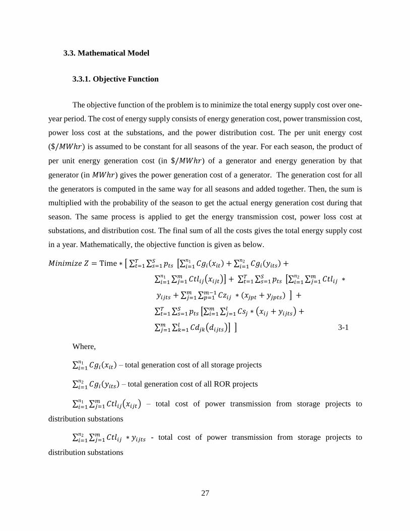
27
3.3. Mathematical Model
3.3.1. Objective Function
The objective function of the problem is to minimize the total energy supply cost over one-
year period. The cost of energy supply consists of energy generation cost, power transmission cost,
power loss cost at the substations, and the power distribution cost. The per unit energy cost
($/𝑀𝑊ℎ𝑟) is assumed to be constant for all seasons of the year. For each season, the product of
per unit energy generation cost (in $/𝑀𝑊ℎ𝑟) of a generator and energy generation by that
generator (in 𝑀𝑊ℎ𝑟) gives the power generation cost of a generator. The generation cost for all
the generators is computed in the same way for all seasons and added together. Then, the sum is
multiplied with the probability of the season to get the actual energy generation cost during that
season. The same process is applied to get the energy transmission cost, power loss cost at
substations, and distribution cost. The final sum of all the costs gives the total energy supply cost
in a year. Mathematically, the objective function is given as below.
𝑀𝑖𝑛𝑖𝑚𝑖𝑧𝑒 𝑍 = Time ∗ [ ∑ ∑ 𝑝𝑡𝑠𝑆𝑠=1
𝑇𝑡=1 [∑ 𝐶𝑔𝑖(𝑥𝑖𝑡)𝑛1
𝑖=1 + ∑ 𝐶𝑔𝑖(𝑦𝑖𝑡𝑠)𝑛2
𝑖=1 +
∑ ∑ 𝐶𝑡𝑙𝑖𝑗(𝑥𝑖𝑗𝑡)𝑚𝑗=1
𝑛1
𝑖=1 ] + ∑ ∑ 𝑝𝑡𝑠𝑆𝑠=1
𝑇𝑡=1 [∑ ∑ 𝐶𝑡𝑙𝑖𝑗 ∗𝑚
𝑗=1𝑛2
𝑖=1
𝑦𝑖𝑗𝑡𝑠 + ∑ ∑ 𝐶𝑧𝑖𝑗 ∗ (𝑥𝑗𝑝𝑡 + 𝑦𝑗𝑝𝑡𝑠)𝑚−1𝑝=1
𝑚𝑗=1 ] +
∑ ∑ 𝑝𝑡𝑠𝑆𝑠=1
𝑇𝑡=1 [∑ ∑ 𝐶𝑠𝑗 ∗ (𝑥𝑖𝑗 + 𝑦𝑖𝑗𝑡𝑠)𝑙
𝑗=1𝑚𝑖=1 +
∑ ∑ 𝐶𝑑𝑗𝑘(𝑑𝑖𝑗𝑡𝑠)𝑙𝑘=1
𝑚𝑗=1 ] ] 3-1
Where,
∑ 𝐶𝑔𝑖(𝑥𝑖𝑡)𝑛1
𝑖=1 – total generation cost of all storage projects
∑ 𝐶𝑔𝑖(𝑦𝑖𝑡𝑠)𝑛2
𝑖=1 – total generation cost of all ROR projects
∑ ∑ 𝐶𝑡𝑙𝑖𝑗(𝑥𝑖𝑗𝑡)𝑚𝑗=1
𝑛1
𝑖=1 – total cost of power transmission from storage projects to
distribution substations
∑ ∑ 𝐶𝑡𝑙𝑖𝑗 ∗ 𝑦𝑖𝑗𝑡𝑠𝑚𝑗=1
𝑛2
𝑖=1 - total cost of power transmission from storage projects to
distribution substations

28
∑ ∑ 𝐶𝑧𝑖𝑗 ∗ (𝑥𝑗𝑝 + 𝑦𝑗𝑝𝑡𝑠)𝑚−1𝑝=1
𝑚𝑗=1 – total cost of power transmission between inter-
substation lines
∑ ∑ 𝐶𝑠𝑗 ∗ (𝑥𝑖𝑗 + 𝑦𝑖𝑗𝑡𝑠)𝑙𝑗=1
𝑚𝑖=1 – total power loss cost at the substation components like
transformers and switching devices
∑ ∑ 𝐶𝑑𝑗𝑘(𝑑𝑖𝑗𝑡𝑠)𝑙𝑘=1
𝑚𝑗=1 – total power distribution from substations to the demand centers
Time − Time of a year in hours = 8760 hours
3.3.2. Constraints
I. Generation capacity: The amount of power (energy) produced by each power plant
𝑖 during season 𝑡 and scenario 𝑠 (𝑥𝑖𝑡 𝑜𝑟 𝑦𝑖𝑡𝑠) must be less than or equal to its
designed full capacity (𝑆𝑖) during that season.
𝑥𝑖𝑡 ≤ 𝑆𝑖 𝑦𝑖𝑡𝑠 ≤ 𝑓𝑖𝑡𝑠 ∗ 𝑆𝑖 ∀ 𝑖, 𝑡, 𝑠 3-2
Also, power (energy) produced by a plant 𝑖 must be equal to total energy
transmitted from a plant 𝑖 to substation 𝑗. i.e. zero energy storage at the power plant at
any season.
∑ (𝑥𝑖𝑗𝑡 − 𝑥𝑖𝑡)𝑚𝑗=1 = 0 ∑ (𝑦
𝑖𝑗𝑡𝑠 − 𝑦
𝑖𝑡𝑠)𝑚
𝑗=1 = 0 ∀ 𝑖, 𝑡, 𝑠 3-3
II. Transmission line capacity (from generation stations to substations) and
Distribution line (from substations to demand center) capacity: The amount of
power (energy) transmitted through a transmission line and distribution line must
be less than the power carrying capacity of the line.
𝑥𝑖𝑗𝑡 ≤ 𝑇𝐿𝑖𝑗 𝑦𝑖𝑗𝑡𝑠 ≤ 𝑇𝐿𝑖𝑗 𝑥𝑗𝑝𝑡 + 𝑦𝑗𝑝𝑡𝑠 ≤ 𝑍𝑗𝑝 𝑑𝑗𝑘𝑡𝑠 ≤ 𝐷𝐿𝑗𝑘 3-4
III. Substation capacity: Total power input at substation 𝑗 must be less than or equal to
the capacity of that substation.

29
∑ 𝑥𝑖𝑗𝑡𝑛1
𝑖=1 + ∑ 𝑦𝑖𝑗𝑡𝑠
𝑛2
𝑖=1 + ∑ (𝑥𝑝𝑗𝑡 𝑚−1𝑝=1 + 𝑦
𝑝𝑗𝑡𝑠) ≤ 𝑆𝑆𝑗 ∀𝑗, 𝑡, 𝑠 3-5
IV. The power that enters a substation should be equal to the power that leaves that
substation. Assume that there is no power loss at substation.
∑ 𝑥𝑖𝑗𝑡𝑛1
𝑖=1 + ∑ 𝑦𝑖𝑗𝑡𝑠
𝑛2
𝑖=1 + ∑ (𝑥𝑗𝑝𝑡𝑚−1𝑝=1 + 𝑦
𝑗𝑝𝑡𝑠) − ∑ (𝑥𝑝𝑗𝑡
𝑚−1𝑝=1 + 𝑦
𝑝𝑗𝑡𝑠) − ∑ 𝑑𝑗𝑘𝑡𝑠
𝑙𝑘=1 = 0
∀𝑗, 𝑡, 𝑠 3-6
V. Demand Constraint: All demand must be met.
∑ 𝑑𝑗𝑘𝑡𝑠 𝑚𝑗=1 ≥ 𝐷𝑘 ∀𝑘, 𝑡, 𝑠 3-7
VI. Power or energy cannot be negative.
𝑥𝑖𝑡 , 𝑦𝑖𝑡𝑠, 𝑥𝑖𝑗𝑡 , 𝑦𝑖𝑗𝑡𝑠, 𝑥𝑗𝑝𝑡 , 𝑦𝑗𝑝𝑡𝑠, 𝑑𝑗𝑘𝑡𝑠 ≥ 0 ∀𝑖, 𝑗, 𝑘, 𝑡, 𝑠 3-8
3.4. Cost Parameter Definition
Generally, the cost of a power plant consists of four parts – associated costs, induced costs,
external costs, and the opportunity cost of water. Associated costs are costs that are associated with
the need to produce power, such as costs of engineering structures and equipment as well as their
operation and maintenance costs. Induced costs are costs that are needed to mitigate the adverse
impact produced by the project on nature, people or existing ground conditions, such as costs of
environmental mitigation measures. Furthermore, there are external costs also that may be needed
for the smooth construction and operation of the project though they may also serve other purposes,
such as new infrastructure development required for accessibility to the project site. In addition,
the opportunity cost of using the natural resource – water - in a hydropower project should be
added to the total cost to reach the full cost or the opportunity cost can be replaced by the fuel cost
in case of power plants like thermal/nuclear generators [43]. To be more general, these costs are
grouped into two categories: Fixed cost and Variable cost.
Fixed cost:
Fixed cost is a one-time cost that is spent during construction and installation and does not
depend on intended loading variation to be served after operation. Fixed cost consists of

30
construction, installation, equipment, land, permits, site developing and preparation, taxes,
insurance, labor, and testing costs. The capital cost of building a generator station varies from
region to region, largely as a function of labor costs and "regulatory costs," which include things
like obtaining siting permits, environmental approvals, and so on. It is important to realize that
building a generation station takes an enormous amount of time. In a state such as Texas (where
building power plants is relatively easy), the time-to-build can be as short as two years. In
California, where bringing new energy infrastructure to fruition is much more difficult (due to
higher regulatory costs), the time-to-build can exceed ten years. Because of these policy
differences there exists an uncertainty in the final cost of erecting power plants.
Variable cost:
The cost which varies with time is variable cost. For example, the operation maintenance
cost of a power plant varies year after year. It is because older plants require more maintenance.
The operational costs and the cost of new components to replace older ones increase due to
economic factors like inflation. Operating costs for power plants include fuel, labor and
maintenance costs. Also, the operating cost depends on how much electricity that the plant
produces over a period of time. The operating cost required to produce each MWh of electric
energy is referred to as the "marginal cost." Fuel costs dominate the total cost of operation for
fossil-fired power plants. For renewables, fuel is generally free (perhaps with the exception of
biomass power plants in some scenarios); and the fuel costs for nuclear power plants are actually
very low. For these types of power plants, labor and maintenance costs dominate total operating
costs [44].
The mathematical formula for the costs used in the optimization model are formulated as
given in the following section. An experimental study is presented in chapter 4 by using the
mathematical model developed in this chapter. The experiments are carried out by using data from
the Integrated Power System Nepal. The Nepal Electricity Authority (NEA) is the only electricity
utility in the country hence all the data needed for the experimental study were obtained from the
utilities website. Following section also describes how each of the parameters can be obtained to
get the per unit energy cost of the power system components.
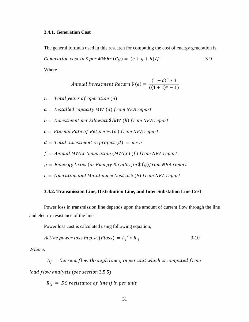
31
3.4.1. Generation Cost
The general formula used in this research for computing the cost of energy generation is,
𝐺𝑒𝑛𝑒𝑟𝑎𝑡𝑖𝑜𝑛 𝑐𝑜𝑠𝑡 𝑖𝑛 $ 𝑝𝑒𝑟 𝑀𝑊ℎ𝑟 (𝐶𝑔) = (𝑒 + 𝑔 + ℎ)/𝑓 3-9
Where
𝐴𝑛𝑛𝑢𝑎𝑙 𝐼𝑛𝑣𝑒𝑠𝑡𝑚𝑒𝑛𝑡 𝑅𝑒𝑡𝑢𝑟𝑛 $ (𝑒) = (1 + 𝑐)𝑛 ∗ 𝑑
((1 + 𝑐)𝑛 − 1)
𝑛 = 𝑇𝑜𝑡𝑎𝑙 𝑦𝑒𝑎𝑟𝑠 𝑜𝑓 𝑜𝑝𝑒𝑟𝑎𝑡𝑖𝑜𝑛 (𝑛)
𝑎 = 𝐼𝑛𝑠𝑡𝑎𝑙𝑙𝑒𝑑 𝑐𝑎𝑝𝑎𝑐𝑖𝑡𝑦 𝑀𝑊 (𝑎) 𝑓𝑟𝑜𝑚 𝑁𝐸𝐴 𝑟𝑒𝑝𝑜𝑟𝑡
𝑏 = 𝐼𝑛𝑣𝑒𝑠𝑡𝑚𝑒𝑛𝑡 𝑝𝑒𝑟 𝑘𝑖𝑙𝑜𝑤𝑎𝑡𝑡 $/𝑘𝑊 (𝑏) 𝑓𝑟𝑜𝑚 𝑁𝐸𝐴 𝑟𝑒𝑝𝑜𝑟𝑡
𝑐 = 𝐸𝑡𝑒𝑟𝑛𝑎𝑙 𝑅𝑎𝑡𝑒 𝑜𝑓 𝑅𝑒𝑡𝑢𝑟𝑛 % (𝑐 ) 𝑓𝑟𝑜𝑚 𝑁𝐸𝐴 𝑟𝑒𝑝𝑜𝑟𝑡
𝑑 = 𝑇𝑜𝑡𝑎𝑙 𝑖𝑛𝑣𝑒𝑠𝑡𝑚𝑒𝑛𝑡 𝑖𝑛 𝑝𝑟𝑜𝑗𝑒𝑐𝑡 (𝑑) = 𝑎 ∗ 𝑏
𝑓 = 𝐴𝑛𝑛𝑢𝑎𝑙 𝑀𝑊ℎ𝑟 𝐺𝑒𝑛𝑒𝑟𝑎𝑡𝑖𝑜𝑛 (𝑀𝑊ℎ𝑟) (𝑓) 𝑓𝑟𝑜𝑚 𝑁𝐸𝐴 𝑟𝑒𝑝𝑜𝑟𝑡
𝑔 = 𝐸𝑒𝑛𝑒𝑟𝑔𝑦 𝑡𝑎𝑥𝑒𝑠 (𝑜𝑟 𝐸𝑛𝑒𝑟𝑔𝑦 𝑅𝑜𝑦𝑎𝑙𝑡𝑦)𝑖𝑛 $ (𝑔)𝑓𝑟𝑜𝑚 𝑁𝐸𝐴 𝑟𝑒𝑝𝑜𝑟𝑡
ℎ = 𝑂𝑝𝑒𝑟𝑎𝑡𝑖𝑜𝑛 𝑎𝑛𝑑 𝑀𝑎𝑖𝑛𝑡𝑒𝑛𝑎𝑐𝑒 𝐶𝑜𝑠𝑡 𝑖𝑛 $ (ℎ) 𝑓𝑟𝑜𝑚 𝑁𝐸𝐴 𝑟𝑒𝑝𝑜𝑟𝑡
3.4.2. Transmission Line, Distribution Line, and Inter Substation Line Cost
Power loss in transmission line depends upon the amount of current flow through the line
and electric resistance of the line.
Power loss cost is calculated using following equation;
𝐴𝑐𝑡𝑖𝑣𝑒 𝑝𝑜𝑤𝑒𝑟 𝑙𝑜𝑠𝑠 𝑖𝑛 𝑝. 𝑢. (𝑃𝑙𝑜𝑠𝑠) = 𝐼𝑖𝑗2 ∗ 𝑅𝑖𝑗 3-10
𝑊ℎ𝑒𝑟𝑒,
𝐼𝑖𝑗 = 𝐶𝑢𝑟𝑟𝑒𝑛𝑡 𝑓𝑙𝑜𝑤 𝑡ℎ𝑟𝑜𝑢𝑔ℎ 𝑙𝑖𝑛𝑒 𝑖𝑗 𝑖𝑛 𝑝𝑒𝑟 𝑢𝑛𝑖𝑡 𝑤ℎ𝑖𝑐ℎ 𝑖𝑠 𝑐𝑜𝑚𝑝𝑢𝑡𝑒𝑑 𝑓𝑟𝑜𝑚
𝑙𝑜𝑎𝑑 𝑓𝑙𝑜𝑤 𝑎𝑛𝑎𝑙𝑦𝑠𝑖𝑠 (𝑠𝑒𝑒 𝑠𝑒𝑐𝑡𝑖𝑜𝑛 3.5.5)
𝑅𝑖𝑗 = 𝐷𝐶 𝑟𝑒𝑠𝑖𝑠𝑡𝑎𝑛𝑐𝑒 𝑜𝑓 𝑙𝑖𝑛𝑒 𝑖𝑗 𝑖𝑛 𝑝𝑒𝑟 𝑢𝑛𝑖𝑡

32
Only dc resistance is considered in this thesis because it is assumed that electrical loads are
active loads and hence the power factor of the power flowing through line is approximately unity.
DC resistance of a transmission line conductor is calculated as:
𝑅𝑡 = 𝑅𝑜(1+ ∝ (𝑡 − 𝑡𝑜))
𝑊ℎ𝑒𝑟𝑒,
𝑅𝑡 = 𝐷𝐶 𝑟𝑒𝑠𝑖𝑠𝑡𝑎𝑛𝑐𝑒 𝑎𝑡 𝑡𝑒𝑚𝑝𝑒𝑟𝑎𝑡𝑢𝑟𝑒 𝑡 ℃
𝑅𝑜 = 𝐷𝐶 𝑟𝑒𝑠𝑖𝑠𝑡𝑎𝑛𝑐𝑒 𝑎𝑡 𝑖𝑛𝑖𝑡𝑎𝑙 𝑡𝑒𝑚𝑝𝑒𝑟𝑎𝑡𝑢𝑟𝑒 𝑡𝑜℃
∝ = 𝑇𝑒𝑚𝑝𝑒𝑟𝑎𝑡𝑢𝑟𝑒 𝑐𝑜𝑒𝑓𝑓𝑖𝑐𝑖𝑒𝑛𝑡 𝑜𝑓 𝑡ℎ𝑒 𝑐𝑜𝑛𝑑𝑢𝑐𝑡𝑜𝑟
Thus the cost associated with power loss in line is calculated as:
𝑃𝑙𝑜𝑜𝑠 𝑖𝑛 𝑀𝑊ℎ𝑟 = 𝑃𝑙𝑜𝑠𝑠𝑖𝑗 ∗ 𝐵𝑎𝑠𝑒 𝑀𝑉𝐴 ∗ 𝑇𝑖𝑚𝑒 𝑖𝑛 ℎ𝑜𝑢𝑟𝑠
Average power purchase rate = $70.30 per 𝑀𝑊ℎ𝑟 (assuming 1$=100 Nepalese rupees (NRs.))
𝑎 = 𝐴𝑛𝑛𝑢𝑎𝑙 (𝑇 𝑎𝑛𝑑 𝐷) 𝑑𝑒𝑝𝑟𝑒𝑐𝑖𝑎𝑡𝑖𝑜𝑛 𝑐𝑜𝑠𝑡 𝑖𝑛 $ (𝑎)
𝑏 = 𝐴𝑛𝑛𝑢𝑎𝑙 𝑜𝑝𝑒𝑟𝑎𝑡𝑖𝑜𝑛 𝑚𝑎𝑖𝑛𝑡𝑒𝑛𝑎𝑛𝑐𝑒 𝑐𝑜𝑠𝑡 𝑖𝑛 $ (𝑏)
𝑐 = 𝑃𝑜𝑤𝑒𝑟 𝑙𝑜𝑠𝑠 𝑐𝑜𝑠𝑡 𝑖𝑛 $ (𝑐) = 𝑃𝑙𝑜𝑠𝑠 𝑖𝑛 𝑀𝑊ℎ𝑟 ∗ 𝐴𝑣𝑒𝑟𝑎𝑔𝑒 𝑝𝑜𝑤𝑒𝑟 𝑝𝑢𝑟𝑐ℎ𝑎𝑠𝑒 𝑟𝑎𝑡𝑒
𝑑 = 𝐻𝑜𝑢𝑟𝑠 𝑖𝑛 𝑎 𝑦𝑒𝑎𝑟 (𝑑) = 8760 hours
𝑒 = 𝑇𝐿 𝑐𝑎𝑝𝑎𝑐𝑖𝑡𝑦 𝑖𝑛 𝑀𝑊 (𝑒)
𝑓 = 𝑇𝑜𝑡𝑎𝑙 𝑐𝑜𝑠𝑡 𝑜𝑓 𝑎 𝑇&𝐷 𝑙𝑖𝑛𝑒 ($/𝑀𝑊ℎ𝑟) (𝑓) = (𝑎 + 𝑏 + 𝑐)/(𝑑 ∗ 𝑒) 3-11
3.4.3. Substation Cost
𝑎 = 𝐴𝑛𝑛𝑢𝑎𝑙 𝑠𝑢𝑏𝑠𝑡𝑎𝑡𝑖𝑜𝑛 𝑑𝑒𝑝𝑟𝑒𝑐𝑖𝑎𝑡𝑖𝑜𝑛 𝑐𝑜𝑠𝑡 𝑖𝑛 $
𝑏 = 𝐴𝑛𝑛𝑢𝑎𝑙 𝑜𝑝𝑒𝑟𝑎𝑡𝑖𝑜𝑛 𝑎𝑛𝑑 𝑚𝑎𝑖𝑛𝑡𝑒𝑛𝑎𝑛𝑐𝑒 𝑐𝑜𝑠𝑡 𝑖𝑛 $
𝑐 = 𝑆𝑢𝑏𝑠𝑡𝑎𝑡𝑖𝑜𝑛 𝑐𝑎𝑝𝑎𝑐𝑖𝑡𝑦 𝑖𝑛 𝑀𝑊
𝑑 = 𝐻𝑜𝑢𝑟𝑠 𝑖𝑛 𝑎 𝑦𝑒𝑎𝑟 = 8760 ℎ𝑜𝑢𝑟𝑠
𝐶𝑜𝑠𝑡 𝑎𝑡 𝑠𝑢𝑏𝑠𝑡𝑎𝑡𝑖𝑜𝑛 ($/𝑀𝑊ℎ𝑟) = (𝑎 + 𝑏)/(𝑐 ∗ 𝑑) 3-12

33
3.5. Resource Capacity Definition
3.5.1. Generation Station Capacity
The electrical power (𝑃 or 𝑆𝑖 in the objective function) in Watts produced from the water
of flow rate (Q) cubic meter per second, and from head height (H) meters is given by the equation
2-1. A hydropower project is very site specific. A particular site for a hydropower project will
produce a specific amount of power and energy that no other site can duplicate. Here are some
lists of parameters that are useful while designing the hydroelectric project (HEP):
Hydraulic Head (H): From above equation 2-1, power produced from hydro energy is
dependent on hydraulic head (H) which varies according to location of power plants. For a constant
discharge, as the values of H increases the electrical power output will also increase. However,
increasing H will increase the length of penstock connecting the headrace and tailrace. Hence, a
comparative study on amount of power increased versus the cost of penstock will give the
economic value of H.
Design discharge (Q): Discharge available in most of the rivers varies monthly due to
change in rainfall pattern and climate change. Generally, HEPs are designed on the basis of the
normal available flow for the river throughout a year. As an example, if a power plant is designed
on the assumption that Q amount of flow will be available 60% of a year then Q60 is the design
discharge of that HEP and it means the power plant will operate at full capacity only during 60%
of the year. Hence, depending upon the project site, design discharge varies like Q45 or Q60 or Q100.
The storage hydroelectric projects are designed to have almost constant discharge (Q) throughout
a year so design discharge of storage HEP is Q100.
In power stations, an electromechanical machine is installed next to the turbine that
regulates water flow (or steam flow in case of a steam turbine) through the turbine blades. This
electromechanical device is called the governor. In other words, the generation limit is determined
by controlling the governor. The following figure shows schematic diagram of a governor.

34
Figure 3.1 Electromechanical governor
The main purpose of governor is to regulate water flow through the turbine based on load
change. If the electrical load on generator increases, speed of the turbine decreases which is sensed
by the governor and it opens the water valve to increase water flow through the turbine blades
resulting in increased speed. Similarly, a decrease in electrical load increases turbine speed and
the governor closes water valve to reduce the water flow and hence reduce the increased speed
back to original value (a reference value). One example of increased load could be, when a ROR
doesn’t supply power to the grid, then the governor in a storage power plant increases water flow
to turbine and hence balances the energy generation and demand.
Capacity of hydroelectric power plants is computed by using equation 2-1. Value of Q and H are
obtained from a field visit to the project site.
3.5.2. Transmission Line, Distribution Line, and Inter Substation Line Capacity
Transmission line and distribution line capacity (TL and DL) is calculated as follows:
𝑃 = ((𝑉𝐿
5.5)
2
−𝑙
6.6) ∗ 𝑐𝑜𝑠(∅) ∗
𝑁𝑐∗150
1000 3-13
𝑆𝐼𝐿 =𝑉𝐿2
𝑍𝑜 3-14
𝑊ℎ𝑒𝑟𝑒,
𝑆𝐼𝐿 = 𝑆𝑢𝑟𝑔𝑒 𝐼𝑚𝑝𝑒𝑑𝑎𝑛𝑐𝑒 𝐿𝑜𝑎𝑑𝑖𝑛𝑔 𝑜𝑓 𝑙𝑖𝑛𝑒
𝑃 = 𝑃𝑜𝑤𝑒𝑟 𝑡𝑟𝑎𝑛𝑠𝑚𝑖𝑡𝑡𝑒𝑑 𝑡ℎ𝑟𝑜𝑢𝑔ℎ 𝑙𝑖𝑛𝑒 𝑖𝑛 𝑀𝑊
𝑙 = 𝐿𝑒𝑛𝑔𝑡ℎ 𝑜𝑓 𝑡𝑟𝑎𝑛𝑠𝑚𝑖𝑠𝑠𝑖𝑜𝑛 𝑙𝑖𝑛𝑒 𝑖𝑛 𝑘𝑚
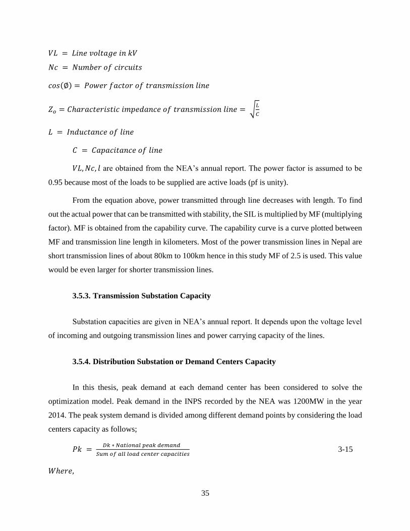
35
𝑉𝐿 = 𝐿𝑖𝑛𝑒 𝑣𝑜𝑙𝑡𝑎𝑔𝑒 𝑖𝑛 𝑘𝑉
𝑁𝑐 = 𝑁𝑢𝑚𝑏𝑒𝑟 𝑜𝑓 𝑐𝑖𝑟𝑐𝑢𝑖𝑡𝑠
𝑐𝑜𝑠(∅) = 𝑃𝑜𝑤𝑒𝑟 𝑓𝑎𝑐𝑡𝑜𝑟 𝑜𝑓 𝑡𝑟𝑎𝑛𝑠𝑚𝑖𝑠𝑠𝑖𝑜𝑛 𝑙𝑖𝑛𝑒
𝑍𝑜 = 𝐶ℎ𝑎𝑟𝑎𝑐𝑡𝑒𝑟𝑖𝑠𝑡𝑖𝑐 𝑖𝑚𝑝𝑒𝑑𝑎𝑛𝑐𝑒 𝑜𝑓 𝑡𝑟𝑎𝑛𝑠𝑚𝑖𝑠𝑠𝑖𝑜𝑛 𝑙𝑖𝑛𝑒 = √𝐿
𝐶
𝐿 = 𝐼𝑛𝑑𝑢𝑐𝑡𝑎𝑛𝑐𝑒 𝑜𝑓 𝑙𝑖𝑛𝑒
𝐶 = 𝐶𝑎𝑝𝑎𝑐𝑖𝑡𝑎𝑛𝑐𝑒 𝑜𝑓 𝑙𝑖𝑛𝑒
𝑉𝐿, 𝑁𝑐, 𝑙 are obtained from the NEA’s annual report. The power factor is assumed to be
0.95 because most of the loads to be supplied are active loads (pf is unity).
From the equation above, power transmitted through line decreases with length. To find
out the actual power that can be transmitted with stability, the SIL is multiplied by MF (multiplying
factor). MF is obtained from the capability curve. The capability curve is a curve plotted between
MF and transmission line length in kilometers. Most of the power transmission lines in Nepal are
short transmission lines of about 80km to 100km hence in this study MF of 2.5 is used. This value
would be even larger for shorter transmission lines.
3.5.3. Transmission Substation Capacity
Substation capacities are given in NEA’s annual report. It depends upon the voltage level
of incoming and outgoing transmission lines and power carrying capacity of the lines.
3.5.4. Distribution Substation or Demand Centers Capacity
In this thesis, peak demand at each demand center has been considered to solve the
optimization model. Peak demand in the INPS recorded by the NEA was 1200MW in the year
2014. The peak system demand is divided among different demand points by considering the load
centers capacity as follows;
𝑃𝑘 = 𝐷𝑘 ∗ 𝑁𝑎𝑡𝑖𝑜𝑛𝑎𝑙 𝑝𝑒𝑎𝑘 𝑑𝑒𝑚𝑎𝑛𝑑
𝑆𝑢𝑚 𝑜𝑓 𝑎𝑙𝑙 𝑙𝑜𝑎𝑑 𝑐𝑒𝑛𝑡𝑒𝑟 𝑐𝑎𝑝𝑎𝑐𝑖𝑡𝑖𝑒𝑠 3-15
𝑊ℎ𝑒𝑟𝑒,

36
𝑃𝑘 = 𝑃𝑒𝑎𝑘 𝑑𝑒𝑚𝑎𝑛𝑑 𝑎𝑡 𝑑𝑒𝑚𝑎𝑛𝑑 𝑐𝑒𝑛𝑡𝑒𝑟 𝑘
𝐷𝑘 = 𝐷𝑖𝑠𝑡𝑟𝑖𝑏𝑢𝑡𝑖𝑜𝑛 𝑠𝑢𝑏𝑠𝑡𝑎𝑡𝑖𝑜𝑛 𝑐𝑎𝑝𝑎𝑐𝑖𝑡𝑦 𝑔𝑖𝑣𝑒𝑛 𝑓𝑟𝑜𝑚 𝑡ℎ𝑒 𝑁𝐸𝐴’𝑠 𝑟𝑒𝑝𝑜𝑟𝑡
𝑆𝑢𝑚 𝑜𝑓 𝑎𝑙𝑙 𝑙𝑜𝑎𝑑 𝑐𝑒𝑛𝑡𝑒𝑟 𝑐𝑎𝑝𝑎𝑐𝑖𝑡𝑖𝑒𝑠 > 𝑁𝑎𝑡𝑖𝑜𝑛𝑎𝑙 𝑝𝑒𝑎𝑘 𝑑𝑒𝑚𝑎𝑛𝑑
In a three-phase power system, active and reactive power flow from the generating station
to the load through the power system components. The system operator has to make sure to balance
total load and generation in the system at every time possible. The optimization model presented
in this thesis considers only active power because the reactive power can be generated locally at
the load center. Some capacitor banks or synchronous machines are directly connected in parallel
with an electrical load that supply the reactive power required by the load locally.
3.5.5. Load Flow Analysis
In addition to supplying energy at minimum cost, the system operator needs to check
whether the network parameters (voltages and power flow in the transmission lines) are within
limit every time when generation or load changes. For example, it might be cheaper to supply
power at minimum cost but the power system voltage or frequency would be out of national grid
limits. The optimal results from the optimization model at off limit voltage and frequency would
not be a practical result. To address this issue, a load flow analysis is performed using Power
System Analysis Toolbox (PSAT) and Matrix Laboratory (MATLAB) tools and results are given
in the appendix section of this thesis. The flow of active and reactive power is called power flow
or load flow. Power flow is a systematic mathematical approach for determination of various bus
voltages, phase angles, active and reactive power flows through different branches, generators and
loads under steady state condition. These parameters are necessary for planning, operation,
economic scheduling and exchange of power between utilities. The principal information of power
flow analysis is to find the magnitude and phase angle of voltage at each bus and the real and
reactive power flowing in each transmission lines [45-48].
Some important terminologies used in the load flow analysis are explained with the help
of an integrated power system network given in Figure 3.2.

37
Figure 3.2 Integrated power system network
The basic load flow equations are given below:
𝑉𝑖 = 1
𝑌𝑖𝑗 [{
(𝑃𝑖+𝑗𝑄𝑖)∗
𝑉𝑖 } − ∑ 𝑌𝑖𝑗 ∗ 𝑉𝑗
𝑁𝑗=1 𝑖≠𝑗
] 3-16
𝑃𝑖 − 𝑄𝑖 = 𝑉𝑖∗ ∑ 𝑌𝑖𝑗 ∗ 𝑉𝑗𝑁𝑗=1 3-17
Where,
𝑌𝑖𝑗 = 𝐴𝑑𝑚𝑖𝑡𝑡𝑎𝑛𝑐𝑒 𝑚𝑎𝑡𝑟𝑖𝑥 (𝑝. 𝑢. ) = 1
𝑍𝑖𝑗 =
1
(𝑅𝑖𝑗 + 𝑗𝑋𝑖𝑗)
𝑅𝑖𝑗 = 𝑅𝑒𝑠𝑖𝑠𝑡𝑎𝑛𝑐𝑒 𝑜𝑓 𝑙𝑖𝑛𝑒 𝑖𝑗 (𝑝. 𝑢. )
𝑋𝑖𝑗 = 𝑅𝑒𝑎𝑐𝑡𝑎𝑛𝑐𝑒 𝑜𝑓 𝑙𝑖𝑛𝑒 𝑖𝑗 (𝑝. 𝑢. )
𝑃𝑖 = 𝐴𝑐𝑡𝑖𝑣𝑒 𝑝𝑜𝑤𝑒𝑟 𝑖𝑛𝑗𝑒𝑐𝑡𝑒𝑑 𝑎𝑡 𝑏𝑢𝑠 (𝑝. 𝑢. )
= 𝐺𝑒𝑛𝑒𝑟𝑎𝑡𝑒𝑑 𝑎𝑐𝑡𝑖𝑣𝑒 𝑝𝑜𝑤𝑒𝑟 𝑎𝑡 𝑏𝑢𝑠 𝑖 (𝑃𝑔𝑖 𝑖𝑛 𝑝. 𝑢. )– 𝐿𝑜𝑎𝑑 𝑎𝑐𝑡𝑖𝑣𝑒 𝑝𝑜𝑤𝑒𝑟 𝑎𝑡 𝑏𝑢𝑠 𝑖 (𝑃𝑙𝑖 𝑖𝑛 𝑝. 𝑢)
𝑄𝑖 = 𝑅𝑒𝑎𝑐𝑡𝑖𝑣𝑒 𝑝𝑜𝑤𝑒𝑟 𝑖𝑛𝑗𝑒𝑐𝑡𝑒𝑑 𝑎𝑡 𝑏𝑢𝑠 (𝑝. 𝑢. )
= 𝐺𝑒𝑛𝑒𝑟𝑎𝑡𝑒𝑑 𝑟𝑒𝑎𝑐𝑡𝑖𝑣𝑒 𝑝𝑜𝑤𝑒𝑟 𝑎𝑡 𝑏𝑢𝑠 𝑖 (𝑄𝑔𝑖 𝑖𝑛 𝑝. 𝑢. )– 𝐿𝑜𝑎𝑑 𝑟𝑒𝑎𝑐𝑡𝑖𝑣𝑒 𝑝𝑜𝑤𝑒𝑟 𝑎𝑡 𝑏𝑢𝑠 𝑖(𝑄𝑙𝑖 𝑖𝑛 𝑝. 𝑢. )
𝑉𝑖 = 𝑃ℎ𝑎𝑠𝑜𝑟 𝑣𝑜𝑙𝑡𝑎𝑔𝑒 𝑎𝑡 𝑏𝑢𝑠 𝑖 (𝑝. 𝑢. ) = |𝑉𝑖| < 𝛿𝑖
|𝑉𝑖| = 𝑀𝑎𝑔𝑛𝑖𝑡𝑢𝑑𝑒 𝑜𝑓 𝑣𝑜𝑙𝑎𝑡𝑔𝑒 𝑎𝑡 𝑏𝑢𝑠 𝑖 (𝑝. 𝑢. )
𝛿𝑖 = 𝑃ℎ𝑎𝑠𝑜𝑟 𝑎𝑛𝑔𝑙𝑒 𝑜𝑓 𝑣𝑜𝑙𝑡𝑎𝑔𝑒 𝑎𝑡 𝑏𝑢𝑠 𝑖 𝑖𝑛 𝑑𝑒𝑔𝑟𝑒𝑒
The terminologies used in load flow analysis are described below:

38
Bus:
A bus is a node at which one or many lines, one or many loads and generators are
connected. In a power system each node or bus is associated with 4 quantities, such as magnitude
of voltage, phage angle of voltage, active or true power and reactive power. In load flow problems
two out of these 4 quantities are specified and remaining 2 are required to be determined by solving
the load flow equations. Depending on the quantities that have been specified, the buses are
classified into 3 categories:
Load Buses: In these buses no generators are connected and hence the generated real power
𝑃𝑔𝑖 and reactive power 𝑄𝑔𝑖 are taken as zero. The objective of the load flow is to find the bus
voltage magnitude |𝑉𝑖| and its angle 𝛿𝑖.
Voltage Controlled Buses: These are the buses where generators are connected. Therefore,
the power generation in such buses is controlled through a prime mover or turbine with governor
while the terminal voltage is controlled through the generator excitation. Keeping the input power
constant through turbine-governor control and keeping the bus voltage constant using automatic
voltage regulator, we can specify constant 𝑃𝑔𝑖 and | 𝑉𝑖 | for these buses.
Slack or Swing Bus: This is a generator bus which is considered as a reference bus for all
the other buses. Since it is the angle difference between two voltage sources that dictates the real
and reactive power flow between them, the particular angle of the slack bus is not important.
However, it sets the reference against which angles of all the other bus voltages are measured. For
this reason, the angle of this bus is usually chosen as 0°. Furthermore, it is assumed that the
magnitude of the voltage of this bus is known and assumed as 1 per unit (p.u.).
Power flow analysis is an important tool involving numerical analysis applied to a power
system. In this analysis, iterative techniques are used due to absence of a known analytical method
to solve the problem. Load flow analysis is used to ensure that electrical power transfer from
generators to consumers through the grid system is stable. Conventional techniques for solving the
load flow problem are iterative, using the Newton-Raphson or the Gauss-Seidel methods.
Once the bus voltages are computed using load flow analysis, power loss in line 𝑖𝑗 is
calculated as:
𝐴𝑐𝑡𝑖𝑣𝑒 𝑝𝑜𝑤𝑒𝑟 𝑙𝑜𝑠𝑠 𝑖𝑛 𝑝. 𝑢. (𝑃𝑙𝑜𝑠𝑠𝑖𝑗) = 𝑅𝑒(𝐼𝑖𝑗 )2 ∗ 𝑅𝑖𝑗 3-18

39
Where,
𝐼𝑖𝑗 (𝑝. 𝑢. ) =(𝑉𝑖 – 𝑉𝑗 )
𝑍𝑖𝑗
Thus the cost associated with power loss in line is calculated as:
Ploss in line ij in MWhr = Ploss in line ij in p. u.∗ Base MVA ∗ Time of operation in hours
In this thesis, the time of operation is 1 year (365days) period. Assuming loss of load factor
(LOLF) of 1 (i.e. load is supplied all the time), total hours in 365 days are:
Time of operation in hours (Time) = 365 ∗ 24 = 8760 hrs
LOLF: It is the ratio of actual energy supplied to a load over a given period of time, to
potential energy that the load could consume without any disturbances over the same period of
time.
LOLF =Actual Energy supplied to a load over a given period of time
Total load capacity∗Total time over the same period 3-19
In a deregulated pool market, the solution of an optimization problem has to serve a double
task. First, the solution aims to minimize the power supply costs. At the same time the solution
needs to meet the load demand as much as possible. Loss of load is the loss in revenue for the
utility as the customers will not pay if they do not get the energy supply. The optimization model
calculates the optimal way of meeting the demand by exploring various combinations of
generators, transmission lines, substations, and distribution lines.

40
CHAPTER 4. NUMERICAL EXPERIMENTS
To address the issue of variability in power generation, a random set of data is generated
in each season. Each set of the random data has random scenarios (number of scenarios depends
on the sample size chosen by the decision maker), these scenarios represent the plant factor of the
ROR power plants (given by 𝑓𝑖𝑡𝑠 in the mathematical model). It is assumed that the data set follows
a uniform distribution during each season. Also, it should be noted that the higher the sample size
for the random scenarios is the more accurate the result will be, with the computation time
increases proportionally. The variation in electrical power generation during a season does not
guarantee the load-generation balance for that time. The ROR power plants which have
Qwet amount of discharge during the wet season may get a water discharge of about one third of
Qwet in the dry season. Hence, from equation 2-1, electrical power generation goes down to one
third of designed capacity during dry season (Qdry) . The stochastic model is expected to address
the uncertainty of energy generation. To address the problem of excess demand (due to the
decreased generation) the deficit power needs to be supplied from some external sources. These
external sources could be the private energy producers within the country (also called independent
power producers) or power purchased from neighboring countries through cross boarder
transmission lines. To discourage the importing energy from external source when it is not needed,
a penalty function is used in the mathematical model. The penalty can be interpreted as the cost
due to importing the unbalanced energy from the external sources. The stochastic model uses an
algorithm called sample average approximation [49].
The computational tool used to solve the model is Gurobi optimizer version 6.0.4 along
with Python software version 2.7 as a programming language. The Gurobi optimizer is a
commercial optimization solver for linear programming, quadratic programming and other types
of mathematical model.
The mathematical model is solved by using data of an existing power system. The
integrated power system chosen for the experimental analysis is Integrated Nepal Power System
(INPS) owned and operated by the government of Nepal. Nepal Electricity Authority, a
government entity, is the only utility in the country which owns and operates major power plants
and all the transmission and distribution network. Some necessary data were collected from the

41
annual reports given in NEA’s website and some data were collected from the Government of
Nepal- Ministry of Energy’s website. The major power plants in the INPS are hydroelectric plants
and some diesel plants as well as solar farms. The reason behind the majority of hydroelectric
projects is that Nepal has more than 6,000 rivers (including rivulets and tributaries) due to glaciers
in the Himalayas, regular monsoon rain, and local topography. These rivers have high water
discharge rates that increases the potential of hydropower generation in the country. The country
has 83,290 MW megawatts (MW) of theoretical hydroelectric potential, about 42,140 MW of
which is technically and economically viable [50]. Also, it is estimated that about 50 MW of
electricity can be generated by installing micro-hydro plants [51].
The river discharge varies with the amount of rain fall, snow fall, and snow melting in the
region of study over a time period. Hydropower is the only resource available to generate
electricity in almost every part of the country, both for large export projects and small village mini
grid projects. Currently, Nepal has both ROR and storage type hydroelectric plants to supply the
current demand. Since the total installed capacity of ROR projects is more than the storage
projects, total power generation from the existing power plants varies monthly which is mainly
due to the seasonal fluctuation of river discharges.
Hydrological seasons in Nepal can be categorized in three different groups: (a) dry pre-
monsoon season (March–May) with almost no rain; (b) rainy monsoon season (June–September);
and (c) post-monsoon season (October–February) with little rain [52]. The average precipitation
in Nepal in mm per year is 1500 mm (59”) [53]. Four months of rainy monsoon season provide
almost 80% rainfall but rest of eight months are almost dry months in the Nepalese rainfall pattern
[54, 55]. As a result, river discharge also shows large seasonal fluctuations closely following the
annual precipitation cycles. The rivers are over flooded during four months of monsoon and power
plants produce full capacity of electrical power, while during the rest of eight months the generated
power goes down to one third of the total capacity [56].
Despite having a large potential of hydropower the country hasn’t been able to harvest the
full potential energy rather the government has been importing power from neighboring country
like India. As the INPS has both variable energy generators (ROR) as well non-variable energy
generators (storage and power purchased from India), it is the best example to use data from and
hence show the practical significance of this thesis. A descriptive map of the INPS showing all the

42
existing power plants, transmission and distribution lines, substations, and demand centers is given
in Appendix A: The Integrated Nepal Power System. The following sections have the data about
major power plant capacity, transmission and distribution lines capacity, substation capacity, and
hourly average value of peak demand in the system. The input data are estimated as follows.
4.1. Model Input Data
4.1.1. Resource Capacity Parameters
A list of the major existing power plants in the INPS and their installed capacity is given
in the following table.
Table 4.1 Existing major hydroelectric power plants and their types (source: NEA [56])
SN Generation stations name
Installed
capacity
in MW
Type
1 Kaligandaki-A (KGA) 144 ROR
2 Lower Marsyandhi (LMRS) and Middle Marsyandhi (MMRS) 139 ROR
3 Kulekhani-I (KL-I) 60 Storage
4 Kulekhani-II (KL-II) 30 Storage
5 Modi (MODI) 24.8 ROR
6 Trishuli (TRSLI) and Chilime (CHLME) 82 ROR
7 Devighat (DVGHT) 14.1 ROR
8 Sunkoshi (SNKSHI) and Indrawati (INDRWTI) 17.55 ROR
9 Khimti (KHMTI) 60 ROR
10 Bhotekoshi (BTKSHI) 45 ROR
11 Dhalkebar (DALKEBAR) 400 Storage
Total
MW
1016

43
As stated earlier, there is a variability in power generation from the ROR projects. Total
energy generation per month is plotted from fiscal year 2010/11 to fiscal year 2014-15 (see
Appendix B: Monthly Power Generation of the Projects). The plant factor of each power plant is
plotted in Figure 4.1.
Figure 4.1 Plant factors of the ROR projects
The Figure 4.1 that maximum power generation occurs during the months of May, June,
July, and August and minimum power generation is during the months of November, December,
January, and February. The actual month of minimum or maximum generation from ROR project
is not same for all fiscal years but time period is approximately same for each year. A sample graph
is given in Figure 4.2.

44
Figure 4.2 Monthly energy generation by the ROR projects
Table 4.2 Nepali to English calendar conversion
Nepali month Equivalent English month
Shrawan July-15 to Aug-15
Bhadra Aug-15 to Sept-15
Ashwin Sept-15 to Oct-15
Kartik Oct-15 to Nov-15
Mangsir Nov-15 to Dec-15
Poush Dec-15 to Jan-15
Magh Jan-15 to Feb-15
Falgun Feb-15 to Mar-15
Chaitra Mar-15 to Apr-15
Baishakh Apr-15 to May-15
Jestha May-15 to June-15
Ashad June-15 to July-15
0.00
20,000.00
40,000.00
60,000.00
80,000.00
100,000.00
120,000.00
FY 2013-2014 Monthly Power Generation of the ROR Projects in
MWhr
Kaligandaki‘A’ Mid-Marsyangdi Marsyandi
Trishuli Gandak Modi
Devighat Sunkoshi

45
In order to get the data as required by the model, the continuously variable energy
generation is grouped into six intervals. Each interval presents a season during which the power
plants generate power at certain percentage of its installed capacity (also called the plant factor or
capacity factor). It should be clear to the reader that the word ‘season’ does not represent the
conventional seasons like winter, summer, or spring. Twelve months are grouped into six seasons
and their plant factors are plotted as shown in the Figure 4.3. Here in this case study, it is assumed
that there are random 5 scenarios of power generation by a power plant during each season. In
other words, the value of 𝑠 (sample size) in the objective function defined in equation 3-1 is 5. The
sample size of 5 is chosen because higher sample size would result longer computation time and also 5
random scenarios for each season give acceptable output results (given in section 4.2).
Figure 4.3 Seasons of a year in the INPS
The Table 4.3 is an example probability table which shows the name of seasons (1 to 6)
and their probabilities of happening in a year. Probability of a season is different for every ROR
project (see Appendix B: Monthly Power Generation of the Projects).

46
Table 4.3 Seasons in a year and their probabilities
Percentage
generation (% of
designed capacity)
Seasons
(s)
Number of
months in
season s
(n)
Chance of
occurrence
(n/12)
Maximum possible
generation during
season ‘s’ (in % of
designed capacity) (fs)
From 100 to 90 1 2 1/6 1
From 90 to 80 2 4 1/3 0.9
From 80 to 70 3 1 1/12 0.8
From 70 to 60 4 2 1/6 0.7
From 60 to 50 5 2 1/6 0.6
From 50 to 40 6 1 1/6 0.5
Each generation station (both ROR and storage) is connected to single or multiple
substations via transmission lines. Then the power is delivered to the demand centers via
distribution lines from the substations. The capacity of exiting transmission and distribution lines
is given in Table 4.4.

47
Table 4.4 Existing transmission and distribution lines capacity in the INPS
PP# Power Plant Capacity
(MW)
Type
(Storage/R
OR)
Substation
connected to
TL line capacity
(kV), length (km),
single or double
circuit
Demand
center
1 Kaligandaki'A' 144
6 hrs
peaking
ROR
Lekhnath
(LKHNTH)
132kV, 65.5 single
circuit
Pokhara
(PKHRA)
2 Kaligandaki'A' 144
6 hrs
peaking
ROR
Butwal
(BTWL)
132kV, 39.1 double
circuit
Butwal
(BTWL)
3
Middle
Marsyangdi 70
5 hrs
peaking
Bharatpur
(BRTPR)
132kV, 38.2 single
circuit
Bharatpur
(BRTPR)
4 Marsyandi 69 ROR
Balaju
(BLJU)
132kV, 83 single
circuit
Kathmandu
(KTM)
5 Marsyandi 69 ROR Bharatpur
132kV, 25 single
circuit
Bharatpur
(BRTPR)
6 Kulekhani I 60 Storage
Hetauda-1
(HTDA-1)
132kV, 7.9 single
circuit
Hetauda-1
(HTDA-1)
7 Kulekhani II 32 Storage
Hetauda-2
(HTDA-2)
132kV, 7.9 single
circuit
Hetauda-2
(HTDA-2)
8 Kulekhani II 32 Storage
Suichatar-1
(SUCH-1)
132kv, 33.4 single
circuit Kathmandu
9 Trishuli 24 ROR
Suichatar-2
(SUCH-2)
66kV, 27.36 double
ciruit Kathmandu
10 ModiKhola 14.8 ROR
Pokhara
(PKHRA)
132kv, 30 single
circuit Pokhara
11 Devighat 15 ROR
Chabel (N-
CHBL)
132kV, 37 single
circuit Kathmandu

48
12 Devighat 15 ROR Balaju
132kV, 27 single
circuit Kathmandu
13 Sunkoshi 10.05 ROR Kathmandu
66kV, 50 single
circuit Kathmandu
14 Ilam(PuwaKhola) 6.2 ROR Illam
33kV, 35 single
circuit Illam
15 Panauti 2.4 ROR Kathmandu
33kV, 20 single
circuit Kathmandu
16 Seti 1.5 ROR Pokhara 11kV Pokhara
17 Fewa 1 ROR Pokhara 11kV Pokhara
18 Sundarijal 0.64 ROR Kathmandu 11kV Kathmandu
19 Pharping 0.5 ROR Kathmandu
11kV, 10 single
circuit Kathmandu
20 Chatara 3.2 ROR Sunsari
33kV, 14 single
circuit Sunsari
21 Gandak 15 ROR Bharatpur
132kV, 20 single
circuit Bharatpur
22 Gandak 15 ROR Bharatpur
132kV, 18 single
ciruit Bharatpur
The Table 4.5 lists the existing substations (both transmission and distribution substations)
and their capacities in Mega Volt Ampere (MVA) as well as average hourly demand at each
demand center. The MVA is a unit to measure capacity of transformers.

49
Table 4.5 Existing substations in the INPS and their capacities
Substations Substation
Capacity MVA Demand points Average Demand MW
LKHNTH and PKHRA 57.5 BRTPR 25
BTWL 142.6 SHVPR 41
BRTPR 30 BARDGHT 51.5
SUCH-1 113.4 CHAPUR 36
HTDA-1 40 HTDA-8 20
HTDA-2 20 TEKU 90
SUCH-2 36 PATN 36
N-CHBL 45 BAN 36
BLJU 90 BALJU 90
LMOSAGU 15 N-CHBL 45
BKTPR 91.5 LNCHR 45
DHLKE 400 LKHNTH / PKHRA 43
Total 1081 Total 558.5
4.1.2. Cost Parameters
The section 3.4 describes how the cost parameters for each power system component are
calculated in this thesis. In addition to the formula given in section 3.4, the following table
summarizes cost parameters used in different literature. The numerical values of costs computed
using above formula are approximately same as in the literature.

50
Table 4.6 Cost parameter computation
Description Literature study data INPS
data Comments and Sources
• Cost of energy from of
ROR generator in $ per
MWhr (Cg)
$7-14 per MWhr in the US,
average of $ 22.62 per MWhr in
France, $40 per MWhr in Australia
$ 6 - 113
per MWhr
http://www.eia.gov/electrici
ty/annual/html/epa_08_04.h
tml
http://bze.org.au/
and from NEA website
• Cost of energy from
storage hydroelectric
power plant in $ per
MWhr (Cg) $7-14 in the US, average of $ 22.62
in France, $40 in Australia
$70.5 per
MWhr
(assuming
$1 = 100
NRs.)
http://www.eia.gov/electrici
ty/annual/html/epa_08_04.h
tml
and from NEA website
• Cost of power loss in
transmission lines from
storage and ROR
generators to substations
in $ per MWhr (Ctl)
$3- 11 per MWhr in European
countries
$1-9 per
MWhr
http://ec.europa.eu/enlarge
ment/archives/seerecon/infr
astructure/sectors/energy/do
cuments/benchmarking/tarif
fs_study.pdf
• Cost of power loss at
substation $ per MWhr
(Cs)
Power loss is very low as compared
to loss in transmission lines and
also depreciation rate of the
equipment is small
$ 2-5 per
MWhr
Load flow analysis of INPS
network
• Cost of power loss in
distribution lines in $ per
MWhr (Cdl) $3- 11 per MWhr in European
countries
$1-3 per
MWhr
Since the length of
distribution line smaller
than transmission line, loss
is low
Finally, all the data presented above were fit into the mathematical model and following results
were obtained.

51
4.2. Analysis of Numerical Results
4.2.1. Operation and Maintenance Cost
Table 4.7 Total operation and maintenance cost from the NEA report
Types of Operating costs FY 2014 FY 2013
Generation Expenses $ 16,792,000.0 $ 16,043,100.0
Power Purchase $ 163,883,100.0 $ 135,724,600.0
Royalty $ 9,300,000.0 $ 8,904,900.0
Transmission Expenses $ 4,500,000.0 $ 4,167,400.0
Distribution Expenses $ 48,555,700.0 $ 40,879,700.0
Depreciation Expenses $ 32,564,800.0 $ 32,286,800.0
Total Operating Expenses $ 275,595,600.0 $ 238,006,500.0
Average $ 256,801,050.0
The solution approaches performed in this research are expectation of expected value
solution (EEV), stochastic solution (SS), and wait and see solution. The analysis of all the three
methods is presented as follows.
4.2.2. Expected Value Solution (EEV)
Expectation of expected value (EEV) model is constructed by replacing the expected value
(EV) with its expectation. The EEV solution is performed in two stages. First, the optimization
problem is solved by using the average of random scenario data (i.e. power generated by ROR
projects during each season scenario) which is called the expected value (EV). This stage of
solution approach provides power generated by both the ROR and storage projects. Since we use
the average of the random scenarios, such an EV model is thus a deterministic optimization
problem because the uncertainty is dealt with before it is introduced to the optimization problem.
Then in second stage, by fixing the values of first stage independent variables (i.e. power generated

52
from storage projects) from the EV problem, the expectation of EV can be obtained by allowing
the optimization problem to choose the values for the random variables (i.e. power generated by
ROR projects).
Power generated by each power plant in MW (Y-axis) during each season of a year (X-
axis) are given in the following graphs:
Table 4.8 Legend
Legend
Kaligandaki A (ROR)
LMrs &MMrs (ROR)
MODI (ROR)
TRSLI & CHLME (ROR)
DVGHT (ROR)
SNKSHI & INDRWTI (ROR)
KHMTI (ROR)
BTKSHI (ROR)
Kulekhani – I (storage)
Kulekhani – II (storage)
From India (Dhalkebar- storage)
0.00
100.00
200.00
300.00
400.00
500.00
600.00
Season
1
Season-1
0.00
100.00
200.00
300.00
400.00
500.00
600.00
Season
2
Season-2

53
Figure 4.4 Decision variable values from EEV approach
As an example, in the above graph for season-1, the power generated by a storage project
(let us say Kulekhani-I) is the average of 5 random values of power generation by the plant. Thus,
the power output from the storage project Kulekhani-I is constant for all scenarios in season-1.
This solution makes the first stage of EV solution. Then, the second stage solution of the EV model
gives the power needs to be generated by a ROR project (let us say Kaligandaki-A) to meet the
total demand. These values are different for each of the 5 scenarios in season-1. The same analysis
is true for other projects as well. The graphs for season-2, 3, 4, 5, and 6 can be interpreted in the
same way. As we take the average of random scenarios in EEV solution, the chances of getting
inaccurate power generation is higher than using the random scenarios themselves. This is the
reason why the total operational cost from EEV solution is higher than SS solution explained in
section 4.2.3.
0.00
100.00
200.00
300.00
400.00
500.00
600.00
Season
3
Season-3
0.00
100.00
200.00
300.00
400.00
500.00
600.00
Season
4
Season-4
0.00
100.00
200.00
300.00
400.00
500.00
600.00
Season
5
Season-5
0.00
100.00
200.00
300.00
400.00
500.00
600.00
Season
6
Season-6

54
Total cost per year obtained from the mathematical model using EV approach = $
113,772,257.8
4.2.3. Stochastic Solution (SS)
In real world problems, the decision variables (power generation, transmission and
distribution here in this case) are uncertain. Their uncertainty can be modeled by a probability
distribution. The solution approach of specifying the uncertainty by using the probability
distributions is called stochastic solution. As the uncertainty requires approximation, the result of
the stochastic solution has some inaccuracies. This research approximates the uncertainties of
future weather conditions (i.e. power output from ROR plants) with a scenario-based approach.
Some random scenarios are generated for each season and such scenarios determines the maximum
capacity of the plant during that season. The scenario size is same as for the EV solution approach.
The graph for season -1 in Figure 4.5 represents the output energy generation in MW (Y-
axis) during first scenario of season 1 (X-axis) and so on.
0
100
200
300
400
500
600
Season 1
Season-1
0
100
200
300
400
500
600
Season
2
Season-2

55
Figure 4.5 Decision variable values from SS approach
The approach shows the total power output from all the generators (both ROR and storage)
from season-1 to season-6. Each scenario of a season is a random number with some probability
of happening. This random number represents the power generated by ROR projects. When the
ROR projects have lower power generation (like in season-6) due to weather change the storage
projects supply the rest of the energy demand. As an example, as the water flow rate decreases
from season-1 to season-6 (given in Figure 4.1) the power purchased from India (a storage project)
increases accordingly shown in Figure 4.5.
0
100
200
300
400
500
600
Season 3
Season-3
0
100
200
300
400
500
600
Season 4
Season-4
0
100
200
300
400
500
600
Season 5
Season-5
0
100
200
300
400
500
600
Season 6
Season-6

56
Total cost per year obtained from the mathematical model using SS approach = $
113,759,512.2 which slightly less than the total cost from EV solution. This makes sense because the second
stage of EV solution approach is same as the SS solution but the first stage considers the average of the
random numbers which is not as accurate as considering the random numbers themselves.
4.2.4. Wait & See Solution (W&S)
The example output from the wait & see algorithm is plotted in the following graphs. The graph
for season-1-1 in Figure 4.6 represents the output energy generation in MW (Y-axis) during first
scenario of season 1 (X-axis) and so on. The wait-and-see solution approach gives the value of the
objective function (i.e. cost of energy supply in this research) if complete information about the
decision variable was known prior to the decision is made. Thus, it can be inferred that the
objective function value is obtained by running each scenario independently as if each scenario
was certain and then final objective function value (cost) would be the average of all the individual
costs. The cost of energy generation obtained from the W&S solution is specific to each scenario
which is always less than the cost obtained if the random scenarios are used like in SS approach.
Total cost per year obtained from the mathematical model using W&S approach = $
112,679,077.76 which cheapest among all three solutions explained above.
0
100
200
300
400
500
600
Season 1
Season-1-1
0
100
200
300
400
500
600
Season 1
Season-1-2

57
0
100
200
300
400
500
600
Season 1
Season-1-3
0
100
200
300
400
500
600
Season 1
Season-1-4
0
100
200
300
400
500
600
Season 6
Season-6-1
0
100
200
300
400
500
600
Season 6
Season-6-2
0
100
200
300
400
500
600
Season 6
Season-6-3
0
100
200
300
400
500
600
Season 6
Season-6-4
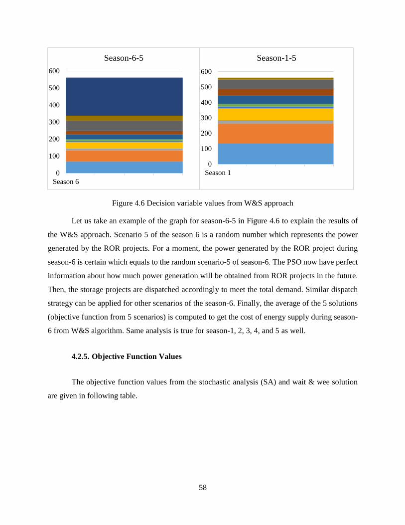
58
Figure 4.6 Decision variable values from W&S approach
Let us take an example of the graph for season-6-5 in Figure 4.6 to explain the results of
the W&S approach. Scenario 5 of the season 6 is a random number which represents the power
generated by the ROR projects. For a moment, the power generated by the ROR project during
season-6 is certain which equals to the random scenario-5 of season-6. The PSO now have perfect
information about how much power generation will be obtained from ROR projects in the future.
Then, the storage projects are dispatched accordingly to meet the total demand. Similar dispatch
strategy can be applied for other scenarios of the season-6. Finally, the average of the 5 solutions
(objective function from 5 scenarios) is computed to get the cost of energy supply during season-
6 from W&S algorithm. Same analysis is true for season-1, 2, 3, 4, and 5 as well.
4.2.5. Objective Function Values
The objective function values from the stochastic analysis (SA) and wait & wee solution
are given in following table.
0
100
200
300
400
500
600
Season 6
Season-6-5
0
100
200
300
400
500
600
Season 1
Season-1-5

59
Table 4.9 The objective function values from SS, W&S, and EEV approach
Season
Stochastic
Solution $ Per
Year
Wait & See $
Per Year
EEV $ Per
Year
VSS in $ Per
Year EVPI in $ Per Year
1 (0.9-1.0) 105,180,286.0 102,505,429.6 105,184,108.6 3,822.6 2,674,856.4
2(0.8-0.9) 106,382,788.9 104,025,860.2 106,382,788.9 - 2,356,928.7
3(0.7-0.8) 112,823,116.0 111,970,603.8 112,873,031.7 49,915.8 852,512.1
4(0.6-0.7) 115,744,467.2 115,337,384.1 115,764,199.6 19,732.4 407,083.1
5(0.5-0.6) 121,375,733.3 121,356,994.1 121,378,736.0 3,002.7 18,739.2
6(0.4-0.5) 121,050,682.2 120,878,194.7 121,050,682.2 - 172,487.5
Average 113,759,512.2 112,679,077.7 113,772,257.8 12,745.5 1,080,434.5
Total annual cost from Table 4.7 is equal to $ 256,801,050.0. This cost represents the cost
of energy supply when considering the total INPS load. Here in this thesis only some major portion
of the total is considered which is only about 45 % of the total national peak load.
Total annual savings = $ 256,801,050.0 * 0.45 - $ 113,759,512.2 = $ 1,800,960.3
Expected Value of Perfect Information (EVPI) - is the absolute value of the difference
between SS and W&S i.e.
EVPI = SS-W&S = $ 1,080,434.5
The significance of EVPI is that it gives information about how much the decision maker
should be willing to pay for the perfect information about the future.
Value of stochastic solution (VSS)- is the difference in the objective function
between the solutions of EEV and SS i.e.
VSS = EV – SS = $ 12,745.5
The significance of VSS is that it gives the possible gain by considering all possible random
scenarios.

60
CHAPTER 5. CONCLUSIONS AND RECOMMENDATIONS
5.1. Conclusions
In this thesis, a stochastic mathematical model was developed for an integrated power
system that consists of both the run-of-river and storage projects. The ROR projects are cheaper
to install and operate than the storage hydroelectric project of the same capacity. Also, the ROR
projects are environmentally friendly compared to the storage projects, because ROR projects have
simple water diversion channel. However, due to the fluctuating energy output from the ROR
power plants they pose a reliability threat to the integrated power system. A mathematical model
that could predict the energy output from the ROR by using the probability of future weather
conditions would help the power system operator to schedule all power plants in an optimal way.
The optimal solution would ensure load and generation balance at all times and also the total cost
of energy supply would be minimum.
The Integrated Nepal Power System consisting of ROR and storage type hydroelectric
power plants was taken as a case study power system in this research. Power produced from the
ROR depends on the available water discharge in the river which varies continuously with weather
conditions. On the other hand, the storage projects are designed to produce power at their installed
capacity independent of the temporary weather change. The operational cost of a power plant is
different from another power plant because of the power plant’s location, its size, and maintenance
cost. As an example, a power plant located in the remote area of a country would require larger
investment due to required civil structures like access roads. This investment cost affects the per
unit energy cost of the power plant during its operation. The generated power from the generators
is supplied to demand centers at distant location via power transmission and distribution lines and
substations. The power loss cost in the lines and substations and their operational and maintenance
cost is not the same for all the components. Power loss in the transmission and distribution lines
depends on the length of the line and diameter of the power carrying conductor. A combination of
a generator, a transmission and distribution line, and a substation to supply a demand could be
cheaper than another combination of the different generators, transmission and distribution lines,
and substations due to the cost difference. In addition to the cost parameters, the power system
components have some constraints like maximum capacity of the component which restricts the

61
further operation of that component even though it would be cheaper to meet the energy demand.
As the number of these power system components increases the possible combination also
increases, which makes the problem of optimal energy supply more complex. The mathematical
model presented in research considered all the possible combinations and solves the model to give
a most economical way of suppling the load by taking into account the system constraints.
The mathematical model developed is called a two-stage stochastic model which consists
of two stages: first stage is to represent the storage type projects and the second stage represents
the ROR projects. This model provided a solution for the amount of power generation,
transmission and distribution over one-year period by the ROR and storage power plants. Power
generated by the storage projects is more certain than the ROR, hence, the probability of power
generation by the storage plants during the study period was considered as unity. In contrast, in
the case of ROR plants one-year period was divided into six seasons based on the past year’s power
generation pattern from the ROR projects. Each season had a certain probability of happening over
the study period and also the power plant could only generate up to a certain percentage of their
installed capacity during that season. The historic data on power generation by the ROR projects
was used to find the probability of occurrence of the season and the maximum capacity of a power
plant during that season.
The problem was solved and comparisons of the stochastic solution (SS), expected value
(EEV), and wait and see (W&S) was made. The results from these solution approaches provided
an economical dispatch of the ROR and storage projects and optimal distribution plan to meet the
energy demand. The PSO should interpret the results from these solution techniques as follows:
The months in a year when the power plants can generate power from 90% to 100% of
their installed capacity were grouped into the season-1. Similarly, the months in a year when the
power plants can generate power from 80% to 90% of their installed capacity were grouped into
the season-2 and so on. The results of the decision variables showed that the power generated by
a ROR plant during season-1 was more than the power generated by the same ROR plant in other
seasons. This means the storage power plants should be operating at minimum capacity and store
some water during season-1 so that the stored water could be used to run the plants at increased
capacity during other seasons. If the domestic generation was not sufficient to meet the energy
demand, then power should be purchased from out of state (like from India in case of INPS).

62
For all the experimental runs, the W&S solution approach provided the least cost plan. The
EEV solution was worse than the SS. The PSO may invest in advanced technology to more
accurately reveal the uncertainties to operate at the W&S operational cost. However, the tradeoff
between using the SS solution and investing in new technologies to operate at W&S solution may
require rigorous feasibility study.
Some of the benefits for the energy users, power producers, and the government from the
proposed methodology are:
1. Reliable power supply for the customers.
2. Optimal use of ROR projects which would reduce the cost and also reduce the
environmental effects caused by storage power plants. This would benefit the power
producers and also the government.
3. Optimal use of available domestic power plants.
4. In addition to the optimal energy generation and distribution planning for an existing
system, the government can use the given mathematical model in energy planning. This
can be achieved by using a forecasted energy demand (in place of current demand) for
a certain planning horizon, the solution of the proposed mathematical model would
give an idea of what should be the strategy of energy generation and distribution in
coming future. If the solution produces an infeasible solution due to greater forecasted
demand than total available generation then the decision maker can virtually place a
new power plant with some estimated operational cost to see what would be the best
way to supply the future need of energy.
In addition to the above benefits, this research adds a contribution to the state-of-art by
presenting the integrated power system network as a two-stage transportation problem and
minimizing the total cost of energy supply to the customers. As given in the literature review
section, various research articles can be found in the field of deterministic, stochastic as well as
large scale optimization that present different objective functions and methodologies of solving
problems. Some major objective functions include the optimal scheduling hydro-thermal unit,
optimization of water content in the reservoir for a storage hydroelectric project, minimization of
carbon emission from power plants, scheduling of electrical loads like electric vehicles and

63
thermostatically controlled loads, and optimal sizing and siting of DGs. These articles present
methodologies for optimization only in the generator side or in demand side. However, this thesis
presents a stochastic optimization methodology that considers all the components of the integrated
power system (i.e. generators, transmission and distribution lines, and substations). Power
produced by the generators and transmitted to the distribution substation makes the first stage of
the problem while the power distributed from the substations to the demand centers makes the
second stage of the two-stage transportation problem.
5.2. Future Work
Here, in this research, the energy demand is assumed to be constant over an hour period
(60 minutes), and the optimal energy supply planning is obtained for one-hour period. This
assumption is because of the fact that the energy demand can change in every fraction of seconds,
and finding an optimal solution with the variable demands, and giving commands to the generators
according to the solution would not be practical. However, if the analysis period is reduced to may
be 15 minutes or 30 minutes from 60 minutes that would make better approximation with the real
load change and more accurate results of optimal energy supply planning. Hence, it is a
recommendation for the future researchers in the field of optimization to add a variable energy
demand along with variable energy generation and use time period less than one-hour. This
research considers the flow of active power only in the network because the reactive power
required by the loads can be supplied locally from reactive power generators. However, the power
system consists of components like transmission lines and transformers which require some
reactive power during their operation. The required reactive power needs to supplied by the
generators in the power system. Hence, an optimal reactive power flow methodology needs to
developed. The future researches in this field are recommended to use complex power (active
power and reactive power) in place of active power presented in this thesis.

64
BIBLIOGRAPHY
[1] W. Allen J., W. Bruce F., and S. Gerald B., Power Generation, Operation and Control, 3rd
ed. Hoboken NJ: Willey, 2014.
[2] K. Daniel and S. Goran, Fundamentals of Power System Economics. UK: John Wiley &
Sons, Ltd, 2004.
[3] G. Charles A. and R. Thaddeus A., Fundamentals of Electrical Engineering. CRC Press,
2012.
[4] P. R. Heyl, "What Is Electricity?," American Institute of Electrical Engineers, Transactions
of the, vol. 55, no. 1, pp. 4-11, 1936.
[5] C. E. Comission. (2012). Energy Story. Available: http://www.energyquest.ca.gov/
[6] D. o. t. A. U.S., Planning and design of hydroelectric power plant structures, C. o. E. Army,
Washington, DC, ed., 1995.
[7] U. S. D. o. t. I. B. o. R. P. R. Office, "Managing Water in the West, Hydroelectric Power,"
Available: http://www.usbr.gov/power/edu/pamphlet.pdf
[8] Y. Gebretsadik, C. Fant, K. Strzepek, and C. Arndt, "Optimized reservoir operation model
of regional wind and hydro power integration case study: Zambezi basin and South Africa,"
Applied Energy, vol. 161, pp. 574-582, 2016.
[9] ENERGY.GOV OFFICE OF Energy Efficiency and Renewable Energy. Available:
http://energy.gov/eere/water/types-hydropower-plants
[10] A. G. Kagiannas, D. T. Askounis, and J. Psarras, "Power generation planning: a survey
from monopoly to competition," International Journal of Electrical Power & Energy
Systems, vol. 26, no. 6, pp. 413-421, 2004.
[11] D. C. Moody, "Ten years of experience with deregulating US power markets," Utilities
Policy, vol. 12, no. 3, pp. 127-137, 2004.
[12] M. Sandsmark and B. Tennbakk, "Ex post monitoring of market power in hydro dominated
electricity markets," Energy Policy, vol. 38, no. 3, pp. 1500-1509, 2010.
[13] D. S. Kirschen, "Demand-side view of electricity markets," Power Systems, IEEE
Transactions on, vol. 18, no. 2, pp. 520-527, 2003.
[14] P. Smita and B. N. Vaidya, "Particle Swarm Optimization based Optimal Power Flow for
reactive loss minimization," Electrical, Electronics and Computer Science (SCEECS),
2012 IEEE Students' Conference on, pp. 1-4, 2012.
[15] P. P. a. G. Natarajan, "Solving Two Stage Transportation Problems,"
[16] B. Saravanan, S. Sikri, K. S. Swarup, and D. P. Kothari, "Unit commitment using DP —
An exhaustive working of both classical and stochastic approach," Power, Energy and
Control (ICPEC), 2013 International Conference on, pp. 382-385, 2013.
[17] R. N. Rodrigues, E. C. Finardi, and E. L. da Suva, "Optimal dispatch of hydro generation
plants via augmented Lagrangian," Power Engineering Society General Meeting, 2005.
IEEE, pp. 2732-2737 Vol. 3, 2005.
[18] D. P. Bertsekas, "On the method of multipliers for convex programming," Automatic
Control, IEEE Transactions on, vol. 20, no. 3, pp. 385-388, 1975.
[19] A. Bensalem, A. Bouhentala, and A. El-Maouhab, "Deterministic Optimal Management
Strategy of Hydroelectric Power Plant," Energy Procedia, vol. 18, pp. 225-234, 2012.

65
[20] Y. Luo, W. Wang, and M. Zhou, "Study on optimal scheduling model and technology
based on RPSO for small hydropower sustainability," Sustainable Power Generation and
Supply, 2009. SUPERGEN '09. International Conference on, pp. 1-5, 2009.
[21] M. Nick, R. Cherkaoui, and M. Paolone, "Stochastic day-ahead optimal scheduling of
Active Distribution Networks with dispersed energy storage and renewable resources,"
Technologies for Sustainability (SusTech), 2014 IEEE Conference on, pp. 91-96, 2014.
[22] A. Subramanian, M. Garcia, A. Dominguez-Garcia, D. Callaway, K. Poolla, and P.
Varaiya, "Real-time scheduling of deferrable electric loads," American Control Conference
(ACC), 2012, pp. 3643-3650, 2012.
[23] Y. G. Hegazy, M. M. Othman, W. El-Khattam, and A. Y. Abdelaziz, "Optimal sizing and
siting of distributed generators using Big Bang Big Crunch method," Power Engineering
Conference (UPEC), 2014 49th International Universities, pp. 1-6, 2014.
[24] L. Xia, X. Qiu, X. Wei, and X. Li, "Research of Distribution Generation Planning in Smart
Grid Construction," Power and Energy Engineering Conference (APPEEC), 2010 Asia-
Pacific, pp. 1-4, 2010.
[25] W. El-Khattam, Y. G. Hegazy, and M. M. A. Salama, "An integrated distributed generation
optimization model for distribution system planning," Power Systems, IEEE Transactions
on, vol. 20, no. 2, pp. 1158-1165, 2005.
[26] Y. Vardanyan and M. Amelin, "The state-of-the-art of the short term hydro power planning
with large amount of wind power in the system," Energy Market (EEM), 2011 8th
International Conference on the European, pp. 448-454, 2011.
[27] neos. (2013). Types of optimization problems. Available: http://www.neos-
guide.org/optimization-tree
[28] K. Suresh and N. Kumarappan, "Generation maintenance scheduling using improved
binary particle swarm optimisation considering aging failures," Generation, Transmission
& Distribution, IET, vol. 7, no. 10, pp. 1072-1086, 2013.
[29] G. C. Pflug and A. Pichler, Multistage Stochastic Optimization. Switzerland: Springer
International Publishing, 2014.
[30] T. Sicong, X. Jian-Xin, and S. K. Panda, "Optimization of Distribution Network
Incorporating Distributed Generators: An Integrated Approach," Power Systems, IEEE
Transactions on, vol. 28, no. 3, pp. 2421-2432, 2013.
[31] J. A. Momoh, S. S. Reddy, and Y. Baxi, "Stochastic Voltage/Var control with load
variation," PES General Meeting | Conference & Exposition, 2014 IEEE, pp. 1-5, 2014.
[32] A. Arce, T. Ohishi, and S. Soares, "Optimal dispatch of generating units of the Itaipu
hydroelectric plant," Power Systems, IEEE Transactions on, vol. 17, no. 1, pp. 154-158,
2002.
[33] K. Antony Arokia Durai Raj and C. Rajendran, "A genetic algorithm for solving the fixed-
charge transportation model: Two-stage problem," Computers & Operations Research,
vol. 39, no. 9, pp. 2016-2032, 2012.
[34] L. Shuangquan, W. Jinwen, and L. Zhong, "Short-Term Hydropower Optimal Scheduling
of Multireservoir System Using a Decomposition Approach," Natural Computation, 2008.
ICNC '08. Fourth International Conference on, vol. 6, pp. 565-570, 2008.
[35] G. Vinasco, D. Tejada, E. F. Da Silva, and M. J. Rider, "Transmission network expansion
planning for the Colombian electrical system: Connecting the Ituango hydroelectric power
plant," Electric Power Systems Research, vol. 110, pp. 94-103, 2014.

66
[36] R. H. Liang and Y. Y. Hsu, "Scheduling of hydroelectric generations using artificial neural
networks," Generation, Transmission and Distribution, IEE Proceedings-, vol. 141, no. 5,
pp. 452-458, 1994.
[37] R. Naresh and J. Sharma, "Hydro system scheduling using ANN approach," Power
Systems, IEEE Transactions on, vol. 15, no. 1, pp. 388-395, 2000.
[38] H. Shyh-Jier, "Enhancement of hydroelectric generation scheduling using ant colony
system based optimization approaches," Energy Conversion, IEEE Transactions on, vol.
16, no. 3, pp. 296-301, 2001.
[39] P. Doganis and H. Sarimveis, "Optimization of power production through coordinated use
of hydroelectric and conventional power units," Applied Mathematical Modelling, vol. 38,
no. 7–8, pp. 2051-2062, 2014.
[40] J. Wu, J. Zhu, G. Chen, and H. Zhang, "A Hybrid Method for Optimal Scheduling of Short-
Term Electric Power Generation of Cascaded Hydroelectric Plants Based on Particle
Swarm Optimization and Chance-Constrained Programming," Power Systems, IEEE
Transactions on, vol. 23, no. 4, pp. 1570-1579, 2008.
[41] J. Zábojník and M. Dvořák, "Power grid simulation model for long term operation
planning," Applied Thermal Engineering, vol. 70, no. 2, pp. 1294-1305, 2014.
[42] H. Y. Yamin, "Review on methods of generation scheduling in electric power systems,"
Electric Power Systems Research, vol. 69, no. 2–3, pp. 227-248, 2004.
[43] U. Gautam and A. Karki, "HYDROPOWER PRICING IN NEPALDEVELOPING A
PERSPECTIVE,"
[44] PENNSTATE. Department of Energy and Mineral Engineering. Available: https://www.e-
education.psu.edu/eme801/node/530
[45] H. K. Mishra, N. R. Karki, and N. Gyawali, "Impact study of Khimti-Dhalkebar 220 kV
Transmission Line on the Operation of Integrated Nepal Power System,"
[46] NPTEL. E-learning courses from the IITs and IISC. Available:
http://nptel.ac.in/courses.php
[47] G. Stamtsis, "Power transmission cost calculation in deregulated electricity market ",
Universität Duisburg-Essen, 2003.
[48] J. J. Grainger and W. D. J. Stevenson, Power System Analysis. Mc-Graw Hill, 1994.
[49] T. Santoso, S. Ahmed, M. Goetschalckx, and A. Shapiro, "A stochastic programming
approach for supply chain network design under uncertainty," European Journal of
Operational Research, vol. 167, no. 1, pp. 96-115, 2005.
[50] yatranepal. Introduction to Nepal. Available:
http://www.yatranepal.com/introductiontonepalnew.htm
[51] S. K.C, S. K. Khanal, P. Shrestha, and B. Lamsal, "Current status of renewable energy in
Nepal: Opportunities and challenges," Renewable and Sustainable Energy Reviews, vol.
15, no. 8, pp. 4107-4117, 2011.
[52] R. H. Sharma and N. M. Shakya, "Hydrological changes and its impact on water resources
of Bagmati watershed, Nepal," Journal of Hydrology, vol. 327, no. 3–4, pp. 315-322, 2006.
[53] T. W. B. Group. (2014). Average precipitation in depth (mm). Available:
http://data.worldbank.org/indicator/AG.LND.PRCP.MM
[54] R. H. Sharma and R. Awal, "Hydropower development in Nepal," Renewable and
Sustainable Energy Reviews, vol. 21, pp. 684-693, 2013.

67
[55] D. W. Burbank, B. Bookhagen, E. J. Gabet, and J. Putkonen, "Modern climate and erosion
in the Himalaya," Comptes Rendus Geoscience, vol. 344, no. 11–12, pp. 610-626,
2012/12// 2012.
[56] N. E. Authority. Nepal Electricity Authority. Available: http://nea.org.np/

68
APPENDIX
Appendix A: The Integrated Nepal Power System
Figure A.1 Integrated Nepal Power System map
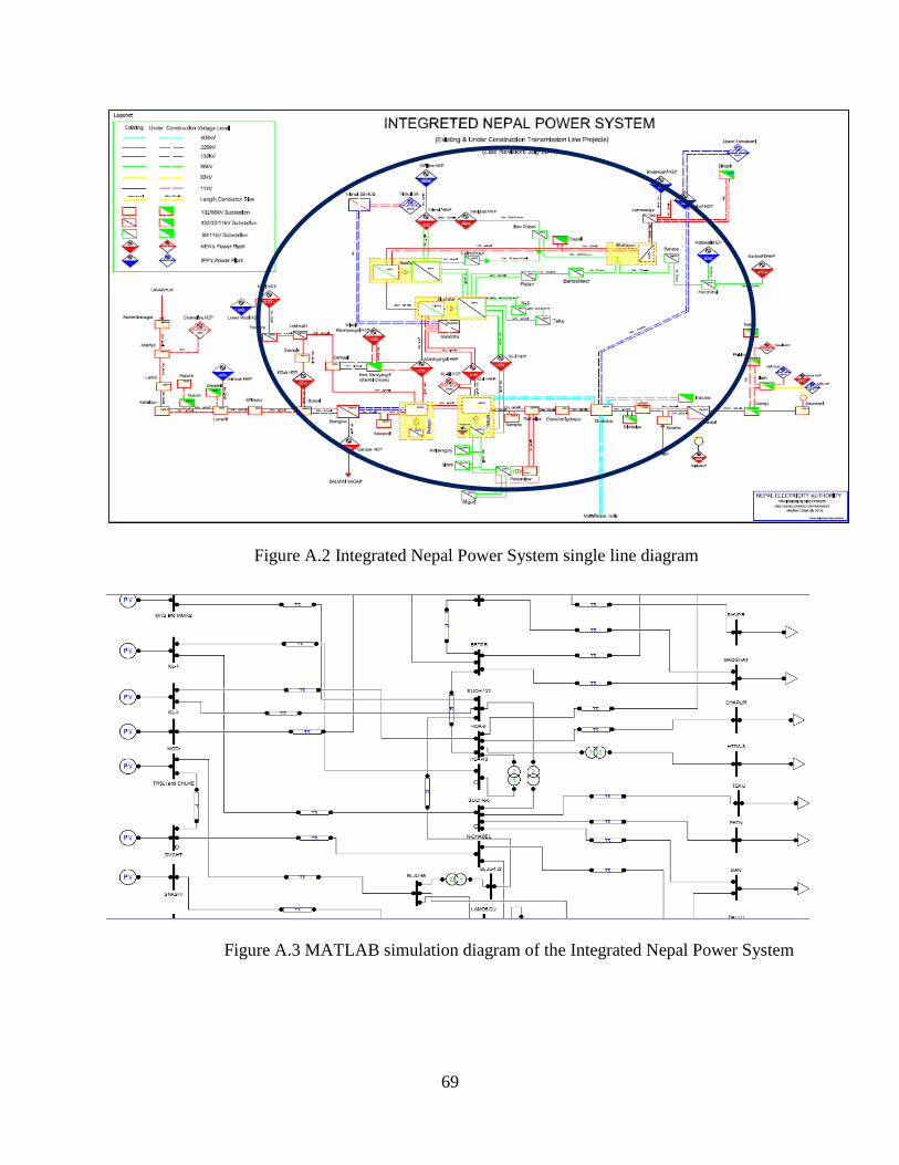
69
Figure A.2 Integrated Nepal Power System single line diagram
Figure A.3 MATLAB simulation diagram of the Integrated Nepal Power System

70
Appendix B: Monthly Power Generation of the Projects
0.00
20,000.00
40,000.00
60,000.00
80,000.00
100,000.00
120,000.00
1 2 3 4 5 6 7 8 9 10 11 12
Kaligandaki‘A’
0.00
10,000.00
20,000.00
30,000.00
40,000.00
50,000.00
60,000.00
1 2 3 4 5 6 7 8 9 10 11 12
Mid-Marsyangdi
0.00
10,000.00
20,000.00
30,000.00
40,000.00
50,000.00
60,000.00
1 2 3 4 5 6 7 8 9 10 11 12
Marsyandi
0.00
2,000.00
4,000.00
6,000.00
8,000.00
10,000.00
12,000.00
1 2 3 4 5 6 7 8 9 10 11 12
Trishuli

71
Figure B.1 Monthly energy generation by the ROR projects in Nepal
0.00
5,000.00
10,000.00
15,000.00
20,000.00
25,000.00
1 2 3 4 5 6 7 8 9 10 11 12
KulekhaniI
0.00
2,000.00
4,000.00
6,000.00
8,000.00
10,000.00
12,000.00
1 2 3 4 5 6 7 8 9 10 11 12
KulekhaniII
0.00
1,000.00
2,000.00
3,000.00
4,000.00
5,000.00
6,000.00
1 2 3 4 5 6 7 8 9 10 11 12
Modi
0.00
500.00
1,000.00
1,500.00
2,000.00
2,500.00
3,000.00
1 2 3 4 5 6 7 8 9 10 11 12
Gandak

72
0.00
50,000.00
100,000.00
150,000.00
200,000.00
250,000.00
FY 2010-2011 Monthly Power Generation of ROR Projects in MWhr
Kaligandaki'A' Mid-Marsyangdi Marsyandi Trishuli
Gandak Modi Devighat Sunkoshi
0.00
50,000.00
100,000.00
150,000.00
200,000.00
250,000.00
FY 2011-2012 Monthly Power Generation of ROR Projects in MWhr
Kaligandaki'A' Mid-Marsyangdi Marsyandi Trishuli
Gandak Modi Devighat Sunkoshi
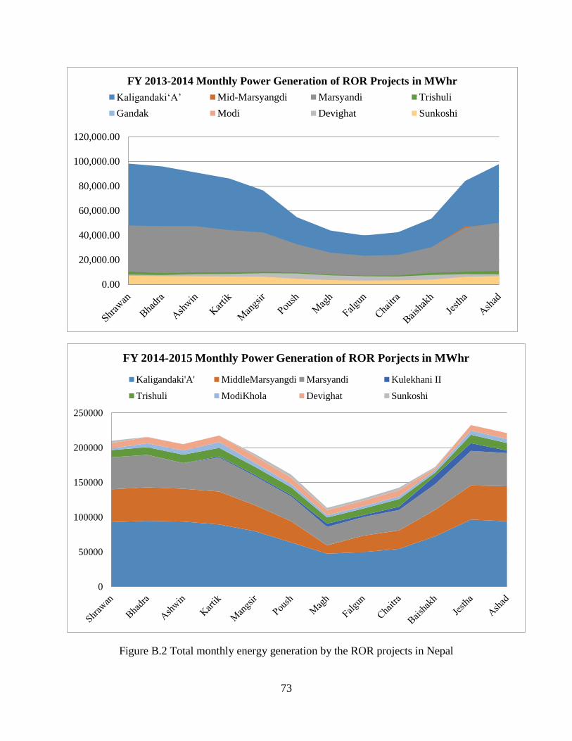
73
Figure B.2 Total monthly energy generation by the ROR projects in Nepal
0.00
20,000.00
40,000.00
60,000.00
80,000.00
100,000.00
120,000.00
FY 2013-2014 Monthly Power Generation of ROR Projects in MWhr
Kaligandaki‘A’ Mid-Marsyangdi Marsyandi Trishuli
Gandak Modi Devighat Sunkoshi
0
50000
100000
150000
200000
250000
FY 2014-2015 Monthly Power Generation of ROR Porjects in MWhr
Kaligandaki'A' MiddleMarsyangdi Marsyandi Kulekhani II
Trishuli ModiKhola Devighat Sunkoshi

74
Figure B.3 Average monthly plant factor or the ROR projects in Nepal (in Percentage)
0.00%
20.00%
40.00%
60.00%
80.00%
100.00%
120.00%
PF
in %
Average Montly Plant Factor of ROR Projects in %
Kaligandaki A
Mid-Marsyangdi andMarsyangdi
Trishuli
Modi
Devighat
Sunkoshi
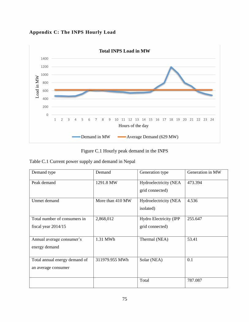
75
Appendix C: The INPS Hourly Load
Figure C.1 Hourly peak demand in the INPS
Table C.1 Current power supply and demand in Nepal
Demand type Demand Generation type Generation in MW
Peak demand 1291.8 MW Hydroelectricity (NEA
grid connected)
473.394
Unmet demand More than 410 MW Hydroelectricity (NEA
isolated)
4.536
Total number of consumers in
fiscal year 2014/15
2,868,012
Hydro Electricity (IPP
grid connected)
255.647
Annual average consumer’s
energy demand
1.31 MWh
Thermal (NEA) 53.41
Total annual energy demand of
an average consumer
311979.955 MWh
Solar (NEA) 0.1
Total 787.087
0
200
400
600
800
1000
1200
1400
1 2 3 4 5 6 7 8 9 10 11 12 13 14 15 16 17 18 19 20 21 22 23 24
Lo
ad i
n M
W
Hours of the day
Total INPS Load in MW
Demand in MW Average Demand (629 MW)

76
Appendix D: Cost and Capacity Parameters Computation
Table D.1 Cost and capacity parameters computation of the power system components
Symbols Literature study data INPS data Comments and Sources
• Number of storage dams (n1) 4
• Number of ROR
hydroelectric generators (n2) 8
• Number of substations (m) 14
• Number of demand and
export regions (l) 12
• Design capacity of
hydroelectric dam (Xi)
Few megawatts (1MW) –
22, 500MW (Three Gorges
Dam in China)
30-200MW
Considering
DHLKEBAR sub-station
as a generation station
• Cost of hydroelectric dam
$7-14 per MW in the US,
average of $ 22.62 per MW
in France, $40 per MW in
Australia
$ 13 - 113 per
MWhr
http://www.eia.gov/electri
city/annual/html/epa_08_
04.html
http://bze.org.au/
and NEA website
• ROR generator design
capacity (Yi)
Few kilowatts (0.1 MW) to
22,5000MW 14-144 MW google.com
• Cost of ROR generator
during construction 100 - 160
dollars per MW
$ 6 - 113 per
MWhr
• Cost of energy from
hydroelectric power plant per
MWhr
$30-100 in the US, average
of $ 22.62 in France, $40 in
Australia
$70.5 per
MWhr
(assuming $1
= 100 NRs.
http://www.eia.gov/electri
city/annual/html/epa_08_
04.html
http://bze.org.au/
and NEA website

77
• Capacity of transmission line
from storage and ROR
generator to substation (TLij)
33kV – 750 kV and
depending upon the length
of power transmission
capacity changes as
described in equation above
33kV - 220 kV
(100 MW to
400MW)
Considering Nepal-India
cross border transmission
line
• Cost of transmission line
from storage and ROR
generator to substation
$3- 11 per MWhr in
European countries
$1-9 per
MWhr
http://ec.europa.eu/enlarg
ement/archives/seerecon/i
nfrastructure/sectors/ener
gy/documents/benchmark
ing/tariffs_study.pdf
• Capacity of substation (Sj)
It can be any depending on
connecting transmission
lines capacities, load center
size 15-143 MW
DHKLEBAR is treated as
a generation station
• Cost of substation
Power loss is very low as
compared to loss in
transmission lines and also
depreciation rate of the
equipment is small
$ 2-5 per
MWhr
Load flow analysis of
INPS network
• Capacity of transmission line
between substations (Spj)
33kV – 750 kV and
depending upon the length
of power transmission
capacity changes as
described in equation above 100MW lines
• Cost of transmission line
between substations
$ 3- 11 per MWhr in
European countries
$1-9 per
MWhr
• Capacity of distribution line
(Ljk)
33kV – 750 kV and
depending upon the length
of power transmission
capacity changes as
described in equation above 100MW lines

78
• Cost of distribution line $3- 11 per MWhr in
European countries
$1-3 per
MWhr
Since the length of
distribution line smaller
than transmission line,
loss is low
• Regional demand distribution
mean (dkω) 20-90 MWhr
• ROR generation sample
uniformly distributed between
60 - 100 percent of the ROR
generator design capacity.

79
Appendix E: Load Flow Analysis Results
Figure E.1 MATLAB and PSAT results for bus voltages in the INPS
In the above figure, all the bus voltages are between 90% to 100% of the rated value. The
range of 0.9 to 1.0 per unit is within the national grid requirement in Nepal. The following figure
shows same analysis for all the 6 seasons of a year.

80
Figure E.2 INPS bus voltage level for each season.