HYDRODYNAMICS BEHAVIOUR OF SLUG FLOW IN 80 OFF THE

HYDRODYNAMICS BEHAVIOUR OF SLUG FLOW IN 800 OFF THE HORIZONTAL PIPE

USING ELECTRICAL CAPACITANCE TOMOGRAPHY (ECT) DATA

A Thesis Presented to the Department of

Petroleum Engineering

The African University of Science and Technology

In Partial Fulfilment of the Requirements

For the Degree of

MASTER OF SCIENCE

By

Dawuda Ismael

Abuja, Nigeria

December, 2014

ii

HYDRODYNAMICS BEHAVIOUR OF SLUG FLOW IN 800 OFF THE HORIZONTAL PIPE

USING ELECTRICAL CAPACITANCE TOMOGRAPHY (ECT) DATA

By

Dawuda Ismael

RECOMMENDED: …………….............................................

Supervisor, Dr. Mukhtar Abdulkadir

…………….............................................

Professor Wumi Iledare

…..............................................................

Dr. Alpheus Igbokoyi

APPROVED: …………….............................................

Chief Academic Officer

…………................................................

DATE.

iii

ACKNOWLEDGEMENT

First of all, I praise almighty God not only for guiding my steps in life but also for providing

me with this opportunity and granting me the capability to proceed successfully.

I extend a hand of appreciation to the African Development Bank for granting me

scholarship for my graduate studies at African University of Science and Technology.

I owe much gratitude to all those people who have made this thesis possible and because of

whom my experience in the graduate program will be forever memorable.

My deepest gratitude goes to my supervisor, Dr. Abdulkadir Mukhtar. I have been lucky to

have a supervisor who gave me the freedom to explore on my own, and at the same time

the guidance to recover when I faltered. Dr. Abdulkadir taught me how to express ideas and

interrogate orthodox ways of doing research. I am most grateful to him not only for

providing me with data and software for my thesis research but also, for training me to be

an independent researcher. It is my hope that I will one day be a sound researcher and a

good supervisor to my students as Dr. Abdulkadir Mukhtar.

My final appreciation goes to parents and siblings for the material and spiritual support they

offered me whiles I was far away from home.

iv

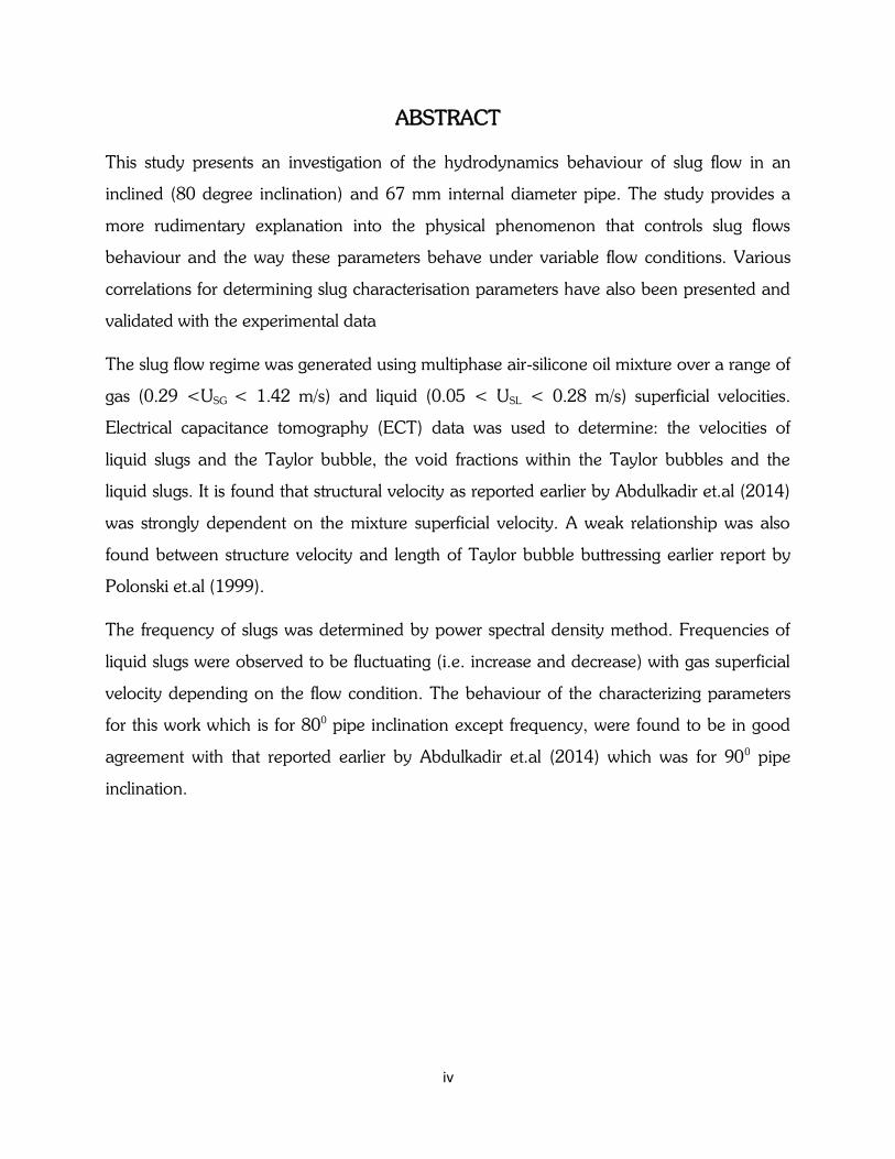
ABSTRACT

This study presents an investigation of the hydrodynamics behaviour of slug flow in an

inclined (80 degree inclination) and 67 mm internal diameter pipe. The study provides a

more rudimentary explanation into the physical phenomenon that controls slug flows

behaviour and the way these parameters behave under variable flow conditions. Various

correlations for determining slug characterisation parameters have also been presented and

validated with the experimental data

The slug flow regime was generated using multiphase air-silicone oil mixture over a range of

gas (0.29 <USG < 1.42 m/s) and liquid (0.05 < USL < 0.28 m/s) superficial velocities.

Electrical capacitance tomography (ECT) data was used to determine: the velocities of

liquid slugs and the Taylor bubble, the void fractions within the Taylor bubbles and the

liquid slugs. It is found that structural velocity as reported earlier by Abdulkadir et.al (2014)

was strongly dependent on the mixture superficial velocity. A weak relationship was also

found between structure velocity and length of Taylor bubble buttressing earlier report by

Polonski et.al (1999).

The frequency of slugs was determined by power spectral density method. Frequencies of

liquid slugs were observed to be fluctuating (i.e. increase and decrease) with gas superficial

velocity depending on the flow condition. The behaviour of the characterizing parameters

for this work which is for 800 pipe inclination except frequency, were found to be in good

agreement with that reported earlier by Abdulkadir et.al (2014) which was for 900 pipe

inclination.

1

Table of contents

ACKNOWLEDGEMENT iii

ABSTRACT iv

Table of contents 1

CHAPTER 1 6

INTRODUCTION 6

1.1 Problem definition 6

1.2 Objective of Research 8

1.3 Method(s) used 8

1.4 Organisation of Thesis 8

CHAPTER 2 10

LITERATURE REVIEW 10

2.1 Introduction 10

2.2 Motion of Taylor bubble in a pipe 10

2.3 Slug frequency 13

2.4 Slug length 15

2.5 Void fraction in the liquid slug 17

CHAPTER 3

DATA COLLECTION, EXPERIMENTAL FACILITY AND DETERMINATION

OF CHARACTERISATION PARAMETERS 19

3.1 Data Collection 19

3.2 The experimental facility 19

3.3 Determination of characterisation parameters for this present study 21

3.3.1 Translational or rise velocity of Taylor bubble (structure velocity) 21

3.3.2. Slug frequency 22

3.3.3 Length of the slug unit, the Taylor bubble and the liquid slug 23

CHAPTER 4 25

RESULTS AND DISCUSSIONS 25

2

4.1 Flow pattern of the regime under study 25

4.2 Structure velocity of Taylor bubble 26

4.3 Effect of bubble length or size on the structure velocity 28

4.4 Void fraction in liquid slug and Taylor bubble. 29

4.5 Total Pressure gradient and frictional pressure gradient 33

4.6 Frequency 37

4.6.1 Comparison of frequency with window function to frequency without window 37

4.6.2 Behaviour of the slug frequency obtained from the experiment. 40

4.6.3 Comparison of experimentally determined frequency against slug frequency obtained

from empirical correlations. 42

4.7 The Length of Taylor bubble and liquid slug 46

4.7.1 The length of slug unit 49

4.7.2 Comparison of liquid slug length obtained from experiment with the correlation

proposed by Khatib and Richardson (1984) 50

CHAPTER 5 52

CONCLUSIONS AND RECOMMENDATIONS 52

5.1 Conclusions 52

5.2 Recommendations 54

References: 55

3

List of figures

Fig 3.1 Inclinable rig 20

Fig 3.2 A schematic of the riser rig 20

Fig 3.3 Void fraction time series from the two ECT probes 22

Fig 4.1 PDF of cross-sectional void fraction of slug flow observed from the experiments

using air-silicone oil. 25

Fig 4.2 Structure velocity determined from experiments and correlations vs mixture

velocity 27

Fig 4.3 Effect of Taylor bubble size on structure velocity 29

Fig 4.4 Void fraction in liquid slug versus gas superficial velocity 31

Fig 4.5 Void fraction in Taylor bubble versus gas superficial velocity 32

Fig 4.6 void fraction in liquid slug versus mean void fraction 33

Fig 4.7 Pressure gradient versus gas superficial velocity 35

Fig 4.8 The influence of the gas superficial velocity on total pressure drop 36

Fig 4.9 The influence of the gas superficial velocity on frictional pressure drop 37

Fig 4.10 Plot of frequency determined with window function against frequency without

window function 39

Fig 4.11 Variation of slug frequency with gas superficial velocity at a various flow

conditions considered in this study 42

Fig 4.12 Variation of slug frequency with gas superficial velocity using results obtained

from experiments and empirical correlations at liquid superficial velocity of 0.05

m/s 43



m/s 44



m/s 44

4



m/s 45



m/s 45

Fig 4.17 Comparison between experimental data frequency and the considered empirical

correlations 46

Fig 4.18 Effect of gas superficial velocity on Taylor bubble length to pipe diameter ratio

for various flows conditions under study 48

Fig 4.19 Effect of gas superficial velocity on liquid slug length to pipe diameter ratio for

various flows conditions under study 49

Fig 4.20 Effect of gas superficial velocity on slug unit length to pipe diameter ratio for

various flows conditions under study 50

Fig 4.21 Comparison between experimental data and Khatib and Richardson (1984)

predictions results 51

5

List of Tables

Table 4.1 Structure velocity determined from experiment and correlations 26

Table 4.2 Void fraction determined from experiment and correlations from Akagawa and

Sakaguchi (1966) and Mori et.al (1999) 30

Table 4.3 Gravitational, frictional and acceleration pressure drop determined from Beggs

and Brill (1973) correlation. 34

Table 4.4 Comparison of frequencies determined with and without window function for

the various flow conditions considered 38

Table 4.5 Summary of results for frequencies obtained from experiment and

correlations. 40

Table 4.6 Summary of void fractions from experiments and correlations, length of liquid

slug, length of Taylor bubble and length of slug unit 47

6

CHAPTER 1

INTRODUCTION

1.1 Problem definition

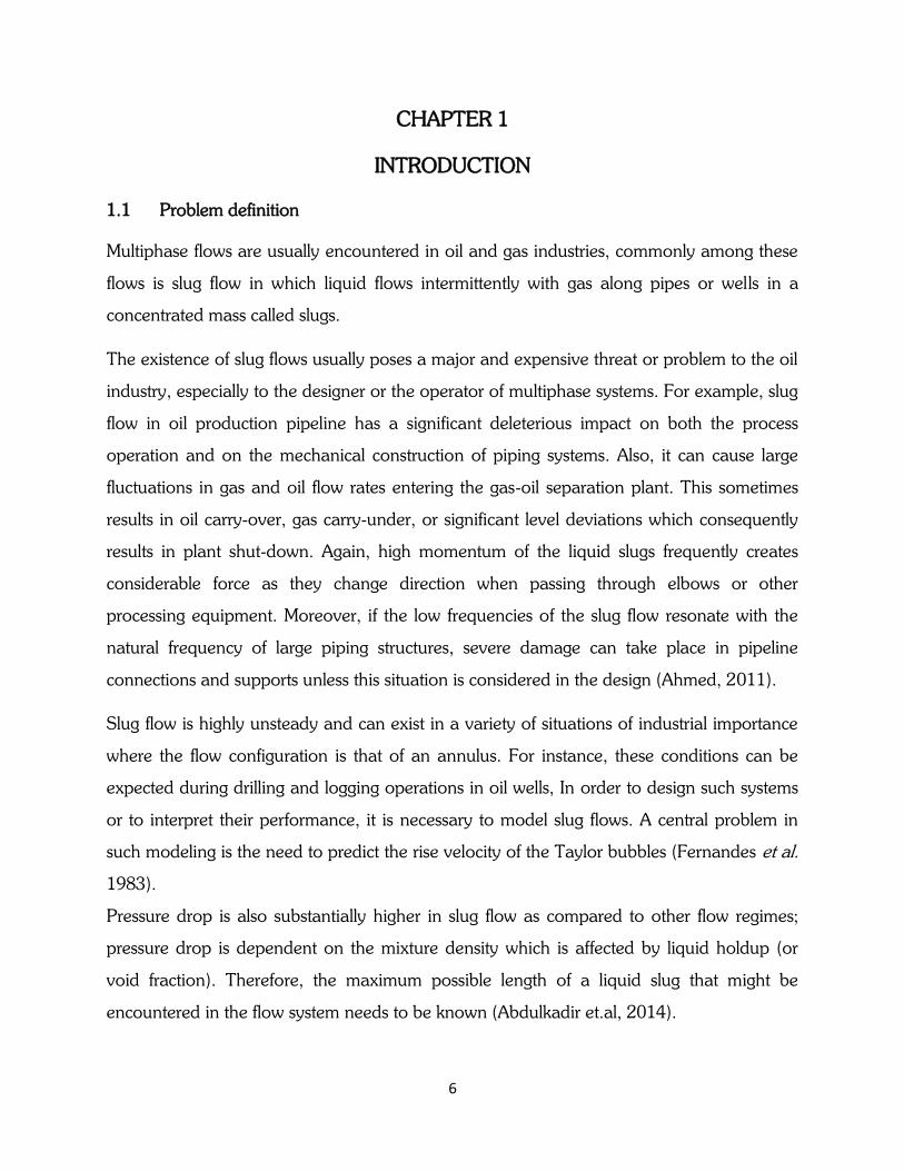
Multiphase flows are usually encountered in oil and gas industries, commonly among these

flows is slug flow in which liquid flows intermittently with gas along pipes or wells in a

concentrated mass called slugs.

The existence of slug flows usually poses a major and expensive threat or problem to the oil

industry, especially to the designer or the operator of multiphase systems. For example, slug

flow in oil production pipeline has a significant deleterious impact on both the process

operation and on the mechanical construction of piping systems. Also, it can cause large

fluctuations in gas and oil flow rates entering the gas-oil separation plant. This sometimes

results in oil carry-over, gas carry-under, or significant level deviations which consequently

results in plant shut-down. Again, high momentum of the liquid slugs frequently creates

considerable force as they change direction when passing through elbows or other

processing equipment. Moreover, if the low frequencies of the slug flow resonate with the

natural frequency of large piping structures, severe damage can take place in pipeline

connections and supports unless this situation is considered in the design (Ahmed, 2011).

Slug flow is highly unsteady and can exist in a variety of situations of industrial importance

where the flow configuration is that of an annulus. For instance, these conditions can be

expected during drilling and logging operations in oil wells, In order to design such systems

or to interpret their performance, it is necessary to model slug flows. A central problem in

such modeling is the need to predict the rise velocity of the Taylor bubbles (Fernandes et al.

1983).

Pressure drop is also substantially higher in slug flow as compared to other flow regimes;

pressure drop is dependent on the mixture density which is affected by liquid holdup (or

void fraction). Therefore, the maximum possible length of a liquid slug that might be

encountered in the flow system needs to be known (Abdulkadir et.al, 2014).

7

Identifying the slug length and slug velocity are important parameters in many practical

applications. For instance, in the oil and gas industry, estimation of maximum slug size or

length is crucial in the design of slug-catchers in the transportation of hydrocarbon two-

phase flow (Ahmed, 2011). Therefore as part of slug characterisation, the maximum

possible slug length or slug size to be anticipated must also be determined for proper design

of separators and their controls to accommodate them.

Extensive work has been carried out on slug flow characterization, some of the most recent

works are those carried by Abdulkadir et.al (2014) on ‘‘experimental study of the

hydrodynamic behaviour of slug flow in a vertical riser using air silicone oil’’ and Ahmed

(2011) on ‘‘experimental investigation of air-oil slug flows through horizontal pipes using

capacitance probes, hot-film anemometer, and image processing’’.

Most models on slug flow characterisation established in literature are based on air and

water, there are limited research works conducted on air and oil. Abdulkadir, (2014) noted

that reports on the study of the behaviour of these slugs in more industry relevant fluids are

limited. For that reason, it is important to study the behaviour of slug flow in great detail for

the optimal, efficient and safe design and operation of two-phase gas–liquid slug flow

systems.

Ahmed (2011) noted that pipe inclination effect continues to be an open question and

recommended that more experimental studies for different pipe inclinations should be

carried out to obtain more reliable slug flow models.

Also, in practice it is rare to have a perfectly horizontal or perfectly vertical pipe or well.

There is some slight deviation from the true vertical or horizontal; therefore characterizing

slug flow for such pipes or wells is worth pursuing.

To satisfy the above reasons, this study seeks to characterize slug flow for a near vertical

pipe (80 degree pipe inclination) using E.C.T data in an attempt to provide more details to

the limited air-oil slug flow models established in literature.

8

1.2 Aim and Objectives of Research

Characterizing slug flow briefly implies determining its velocity, void fraction, frequency

and length or size of the slugs. This study aims to study the hydrodynamics behaviour of

slug flow for a near vertical pipe (80 degree pipe inclination) using E.C.T data in an

attempt to provide more details to the limited air-oil slug flow models established in

literature. In order to meet the aim of the study the following objectives will be met.

To characterize slug flow using available ECT data

To explain how slug flow characterisation parameters behave under various flow

conditions

To validate some empirical correlations established in literature with experimental

data and establish the level of agreement of these correlations with the experimental

data.

To find out whether the characterisation parameters are affected by inclination and

flow conditions or fluid properties

1.3 Method(s) used

Use of electrical capacitance tomography (E.C.T) data to determine the velocities of

Taylor bubbles and liquid slugs, slug frequencies, length of Taylor bubbles and length

of liquid slugs, void fractions within the Taylor bubbles, and liquid slugs.

Use of power spectral density to determine slug frequency

1.4 Organisation of Thesis

The thesis is structured into five chapters as described below and some other relevant

information is provided in the appendices:

Chapter 1 constitutes the problem definition, objectives of the research, methods used and

thesis structure.

Chapter 2 presents the literature review of published papers on various slug flow

characterisation parameters.

Chapter 3 describes in brief the method used and the experimental facility.

9

Chapter 4 details the determination of characterisation parameters and treatment of

findings. Also details analyzed experimental results and how they have been used to

validate some slug flow empirical correlations established in literature.

Chapter 5 is a summary, restating the developments of previous chapters and showing

succinctly the findings, conclusions of the whole study. It also offers some recommendations

10

CHAPTER 2

LITERATURE REVIEW

2.1 Introduction

Several models are found in literature for characterizing slug flow in pipes. These include

both empirical correlations and mechanistic models. This chapter presents a review on the

various slug flow characterisation parameters. A portion of this work has been reviewed in

earlier works by Abdulkadir et.al (2014), Barnea and Taitel (1993), Collins (1978), Cai et al

(1999), Kelessidisi and Duckler (1989) and Polonski et.al (1999)

2.2 Motion of Taylor bubble in a pipe

The study of the motion of Taylor bubbles through a stagnant liquid has generated a vast

literature, starting with the pioneering contribution of Dumitrescu (1943) based on potential

flow of vertical case around an axisymmetric cylinder having a round nose. Other

contributions based on potential flow approach since that time are those of Davies & Taylor

(1950), Collins (1965), Bendiksen (1985) and Nickens & Yanitell (1987) with many others

in between. All these showed the existence of multiple solutions. However, by assuming the

shape of the nose to be approximately spherical, all of these approaches produced a result

similar to

gDkUo (2.10)

Where Uo is drift velocity, K is drift velocity co-efficient, g is acceleration due to gravity and

D is inner pipe diameter.

The value of K is not exact, Different researchers have reported different K values for air-

water system:

Dumitrescu (1943) found that the value of the co-efficient, K (called drift co-efficient) in

equation (2.10) is equal to 0.351. This is very close to the value of K suggested by Stewart

11

and Davidson (1967) to be 0.35. Davies and Taylor (1950) reported K to be 0.346.

According to Clift et.al (1978), the value of K is in the range 0.33-0.36., 0.33-0.38 by

Goldsmith and Manson (1962).

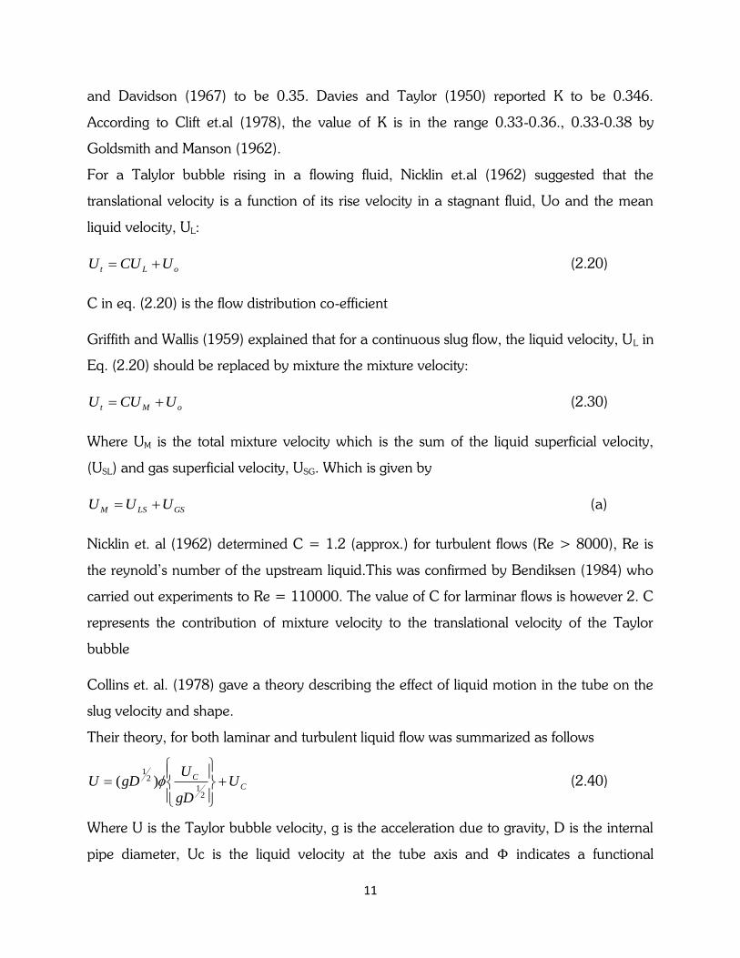
For a Talylor bubble rising in a flowing fluid, Nicklin et.al (1962) suggested that the

translational velocity is a function of its rise velocity in a stagnant fluid, Uo and the mean

liquid velocity, UL:

oLt UCUU (2.20)

C in eq. (2.20) is the flow distribution co-efficient

Griffith and Wallis (1959) explained that for a continuous slug flow, the liquid velocity, UL in

Eq. (2.20) should be replaced by mixture the mixture velocity:

oMt UCUU (2.30)

Where UM is the total mixture velocity which is the sum of the liquid superficial velocity,

(USL) and gas superficial velocity, USG. Which is given by

GSLSM UUU (a)

Nicklin et. al (1962) determined C = 1.2 (approx.) for turbulent flows (Re > 8000), Re is

the reynold’s number of the upstream liquid.This was confirmed by Bendiksen (1984) who

carried out experiments to Re = 110000. The value of C for larminar flows is however 2. C

represents the contribution of mixture velocity to the translational velocity of the Taylor

bubble

Collins et. al. (1978) gave a theory describing the effect of liquid motion in the tube on the

slug velocity and shape.

Their theory, for both laminar and turbulent liquid flow was summarized as follows

C

C U

gD

UgDU

21

21

)( (2.40)

Where U is the Taylor bubble velocity, g is the acceleration due to gravity, D is the internal

pipe diameter, Uc is the liquid velocity at the tube axis and Φ indicates a functional

12

relationship.Their theory provides a strong support for the deduction by Nicklin et. al.

(1962) leading to equation 2.2

Tung and Parlange (1976) and Bendiksen (1985) analyzed the influence of surface tension

on the bubble velocity in the inertial regime, first in stagnant liquid and then in upward flow.

Surface tension was found to decrease the bubble velocity, up to a stationary bubble if

surface tension is high enough. However, in most practical applications surface tension is

negligible. Bendiksen (1985) found that surface tension reduces the rise velocity. He

proposed the following equation

oo

E

E

oEEe

eEC

o

8.61

201

)52.01(

9.01344.0)90,,(

2/30165.0

0165.00

0

(2.50)

Goldsmith and Mason (1962) made an attempt to measure the velocity profiles directly in

front of the bubble and in the liquid film by tracing aluminum particle displacements in still

photographs of the flow. The inception of the reverse flow in the liquid film was observed.

The results agreed well with their model.

Kvernvold et al. (1984) used LDV-technique for measuring the velocity profiles at a limited

number of cross-sections in the slug and in the liquid film in horizontal slug flow.

Nakoryakov et al. (1986, 1989) performed a more extensive study of the instantaneous

velocity field and shear stresses in vertical slug flow by means of an electrochemical velocity

probe. Radial and axial velocity profiles were obtained. Mao and Dukler (1989) measured

the distribution of the wall shear stress in vertical slug flow. They demonstrated a double

change in the flow direction in a slug unit: close to the bubble nose where the film formation

begins; and in the beginning of the liquid slug where the mixing zone ends. The axial

locations of the onset and termination of the reverse flow were close to those measured by

Nakoryakov et al. (1986, 1989).

DeJesus et al. (1995), Kawaji et al. (1997) and Ahmad et al. (1998) applied the

photochromic dye activation method to measure the flow field around a bubble rising in

stagnant liquid (kerosene). The instantaneous velocity distributions in front of the bubble, in

13

the liquid film and in the near wake were visualized. In addition, averaged velocity profiles

in the liquid film were presented. Mao and Dukler (1990, 1991) performed numerical

simulations to calculate the velocity field in front of the bubble and in the liquid film. Clarke

and Issa (1992, 1993) and Bugg et al. (1998) calculated the complete flow field around a

bubble rising in stagnant liquid.

Gas-liquid slug flow is characterized by the presence of a clearly seen moving interface. This

feature makes the flow visualization methods an obvious choice for the measurement

technique. Tassin and Nikitopolous (1995), Lunde and Perkins (1995) and Donevski et al.

(1995) proposed methods based on video imaging and digital image processing for

measuring shape, size and velocity of bubbles in a large volume of liquid. Polonsky et al.

(1999) applied this technique to obtain detailed quantitative data on the instantaneous

characteristics of the bubble motion. (Polonski et.al., 1999)

This study seeks to determine experimentally the velocities of the Taylor bubbles and liquid

slugs using Electrical capacitance tomography (ECT) data.

2.3 Slug frequency

Hubbard (1965) was the first to perform detailed experimental investigations on slug

frequencies. He investigated the flow of air and water in a horizontal pipe where he pointed

out that the frequency of liquid slugs increased with increasing superficial water velocity. His

results were confirmed by experimental investigations of Gregory and Scott (1969) and

Taitel and Duckler (1977). Gregory and Scott (1969) based on their experimental results

proposed the following model for predicting slug frequency

2.122 /36

0157.0

t

t

sl

s VV

sm

gd

Vf (2.60)

Where tV , slV , g and d are translational velocity, liquid superficial velocity, acceleration due

to gravity and pipe diameter respectively

14

Troconi (1990) obtained a correlation for calculating slug frequency with his experimental

results based on the theory of finite amplitude waves originally developed by Kordyban and

Ranov (1970) and by Mishima and Ishii (1980). Troconi’s assumption was that waves on a

liquid surface would grow but only waves characterized by a critical growth rate cause the

formation of a stable liquid slug. His correlation for slug frequency is as follows:

Gf

GGws

h

VCf

1305.0 (2.70)

hG is the height of gas phase layer in a stratified flow, VG is the average gas velocity within

the gas layer cross section of the pipe, G and f are the densities of the gas phase and

liquid film and wC is called proportionality factor (it has a value of 2)

Hill and Wood (1990) also proposed the following model for predicting slug frequency

based on their experimental results. Their model was based on the equilibrium film height.

d

h

m

sd

Vf

68.2

10275.0 (2.80)

Where Vm is mixture velocity, d is pipe diameter and h, is film height

Cai et. al. (1999) proposed a new model for slug frequency prediction based on their

experimental results and Gregory and Scott (1969). Their experiment was carried out at

atmospheric pressure with water and carbon dioxide as working fluids. They identified that

film height (h) in eq. (2.70) as proposed by Hill and Wood (1990) is difficult to measure,

also they identified that Troconi’s model does not account for effect of pipe diameter on

slug frequency and lastly they identified that the model proposed by Gregory and Scott

(1969) does not reflect pipe inclination effect on frequency. Cai et.al proposed a model that

reflects effect pipe inclination and pipe diameter.

2.122 /36

t

t

sl

s VV

sm

gd

VKf (2.90)

Where K is the function of inclination, which reflects the effect of inclination on slug

frequency, Based on their experimental results K can be calculated as follows

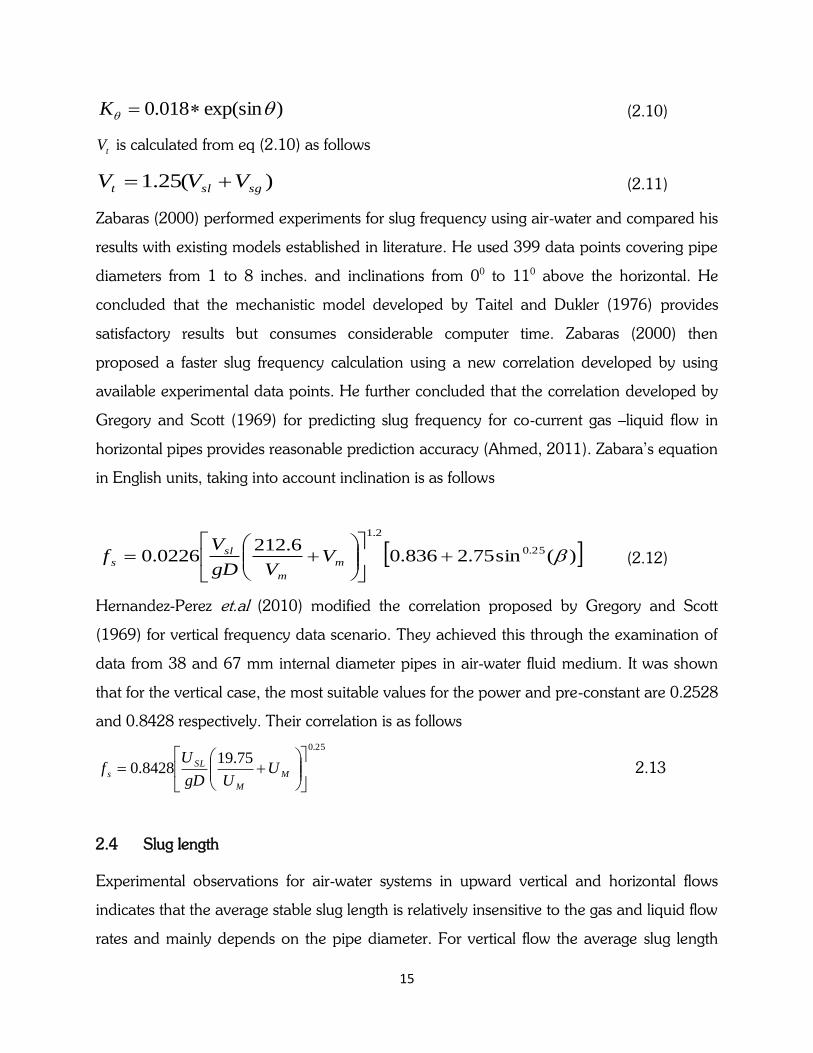
15

)exp(sin018.0 K (2.10)

tV is calculated from eq (2.10) as follows

)(25.1 sgslt VVV (2.11)

Zabaras (2000) performed experiments for slug frequency using air-water and compared his

results with existing models established in literature. He used 399 data points covering pipe

diameters from 1 to 8 inches. and inclinations from 00 to 110 above the horizontal. He

concluded that the mechanistic model developed by Taitel and Dukler (1976) provides

satisfactory results but consumes considerable computer time. Zabaras (2000) then

proposed a faster slug frequency calculation using a new correlation developed by using

available experimental data points. He further concluded that the correlation developed by

Gregory and Scott (1969) for predicting slug frequency for co-current gas –liquid flow in

horizontal pipes provides reasonable prediction accuracy (Ahmed, 2011). Zabara’s equation

in English units, taking into account inclination is as follows

)(sin75.2836.06.212

0226.0 25.0

2.1

m

m

sl

s VVgD

Vf (2.12)

Hernandez-Perez et.al (2010) modified the correlation proposed by Gregory and Scott

(1969) for vertical frequency data scenario. They achieved this through the examination of

data from 38 and 67 mm internal diameter pipes in air-water fluid medium. It was shown

that for the vertical case, the most suitable values for the power and pre-constant are 0.2528

and 0.8428 respectively. Their correlation is as follows

25.0

75.198428.0

M

M

SL

s UUgD

Uf 2.13

2.4 Slug length

Experimental observations for air-water systems in upward vertical and horizontal flows

indicates that the average stable slug length is relatively insensitive to the gas and liquid flow

rates and mainly depends on the pipe diameter. For vertical flow the average slug length

16

gas been observed to be about 8 to 25 pipe diameters Moissis and Grifith (1962), Moissis

(1963), Akagawa and Sakaguchi (1966), Fernandes (1981), Barnea and Shemer, (1989).

Moissis and Grifith (1962), Taitel et al. (1980) and Barnear and Brauner (1985) between

the film and the slug by a wall jet entering a large reservoir. It was suggested that a

developed slug length is equal to the distance at which the jet has been absorbed by the

liquid

Duckler (1985) on the other hand solved boundary layer equations for calculating the

developed slug length. Although the two approaches are different the final results are

similar. Shemer and Barnea (1987) detected the velocity field in the wake of the bubble

using the hydrogen bubble technique and utilized the results for estimating the, minimum

stable slug length. Fabre and Line (1992) found out that slug length is widely dispersed

around its average.

Van Hout et al (1992) measured slug length distribution in upward vertical flow and found

that the ratio between standard deviation and the average is within 20-40%

Brill et al. (1981) based on the data from the Prudhoe Bay field, were the first to suggest

slug length distribution follows a loq-normal distribution for large pipe diameters. Nydal et

al. (1992) measured the statistical distributions of some slug characteristics in air-water

horizontal system and showed that, cumulative probability density function of measured

slug lengths fits a lo-normal distribution well. Bernicot and Drouffe (1989) proposed a

probabilistic approach for slug formation at the entrance of horizontal pipe. They also

model the evolution of the length distribution by an individual equation for each slug. Their

approach is based on the concept that shedding for short slugs is greater than that for long

slugs. Saether et al. (1990) analyzed data from different horizontal two- and three-phase

pipe systems and concluded that the liquid slug length distribution obeys fractal statistics.

Dhulesa et al. (1991) used a 1-D Brownian motion with drift theory to obtain the stable slug

length distribution. Barnea and Taitel (1993) observed that there were cases where there is

insufficient information and much more information concerning slug length distribution, the

mean slug length and maximum possible slug length is essential. They presented a model

that is able to predict slug length distribution at any point along a pipe. Their model

assumes a random distribution at the pipe inlet and calculates the increase or decrease in

17

individual slug length, including disappearance of short slugs as they move downstream.

Their results show that for a fully developed slug flow the mean slug length is about 1.5

times the minimum stable slug length and the maximum length is about 3 times the

minimum stable slug length.

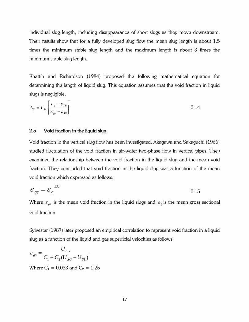
Khattib and Richardson (1984) proposed the following mathematical equation for

determining the length of liquid slug. This equation assumes that the void fraction in liquid

slugs is negligible.

TBgs

TBg

SUS LL

2.14

2.5 Void fraction in the liquid slug

Void fraction in the vertical slug flow has been investigated. Akagawa and Sakaguchi (1966)

studied fluctuation of the void fraction in air-water two-phase flow in vertical pipes. They

examined the relationship between the void fraction in the liquid slug and the mean void

fraction. They concluded that void fraction in the liquid slug was a function of the mean

void fraction which expressed as follows:

8.1

ggs 2.15

Where gs is the mean void fraction in the liquid slugs and g is the mean cross sectional

void fraction

Sylvester (1987) later proposed an empirical correlation to represent void fraction in a liquid

slug as a function of the liquid and gas superficial velocities as follows

)(21 SLSG

SG

gsUUCC

U

Where C1 = 0.033 and C2 = 1.25

18

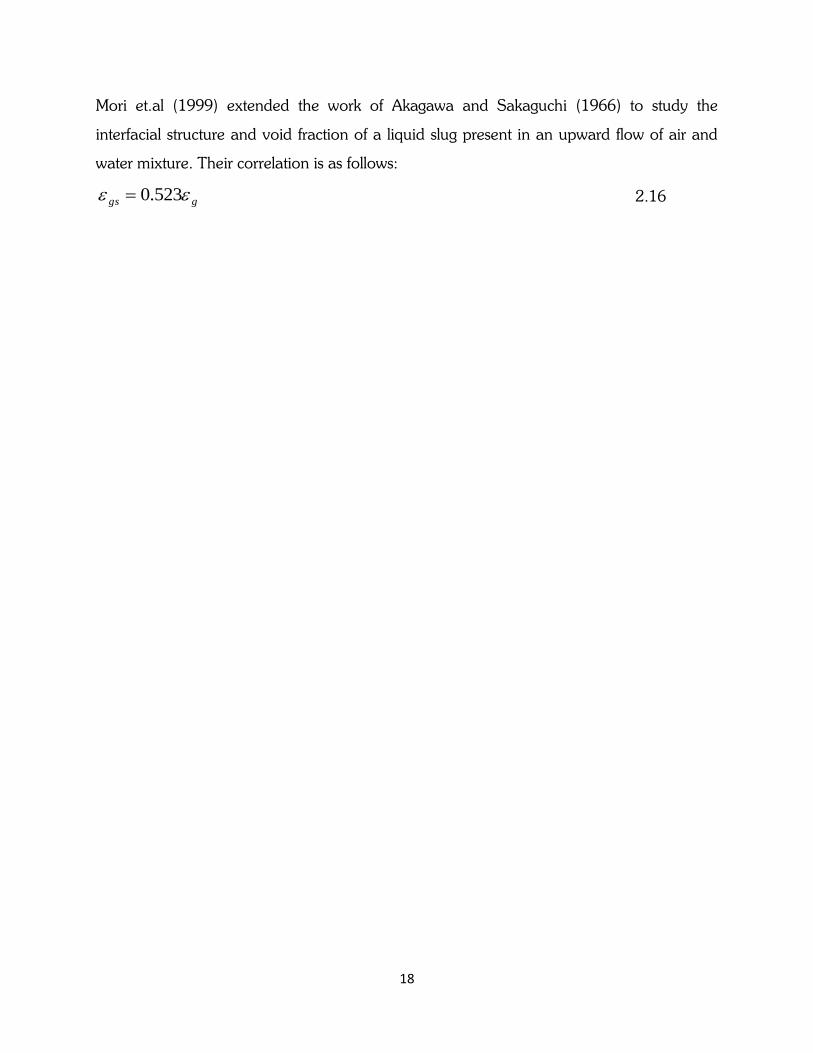
Mori et.al (1999) extended the work of Akagawa and Sakaguchi (1966) to study the

interfacial structure and void fraction of a liquid slug present in an upward flow of air and

water mixture. Their correlation is as follows:

ggs 523.0 2.16

19

CHAPTER 3

DATA COLLECTION, EXPERIMENTAL FACILITY AND DETERMINATION

OF CHARACTERISATION PARAMETERS

3.1 Data Collection

The main data collected for this work was electrical capacitance tomography (ECT) data.

The ECT data was obtained from the data base of University of Nottingham, United

Kingdom. The data obtained was in the form of void fraction time series recorded by the

two electrical capacitance probes. With the ECT data the following parameters were

calculated

The velocities of Taylor bubbles and liquid slugs

Slug frequencies,

Length of Taylor bubbles and length of liquid slugs

Void fractions within the Taylor bubbles, and liquid slugs

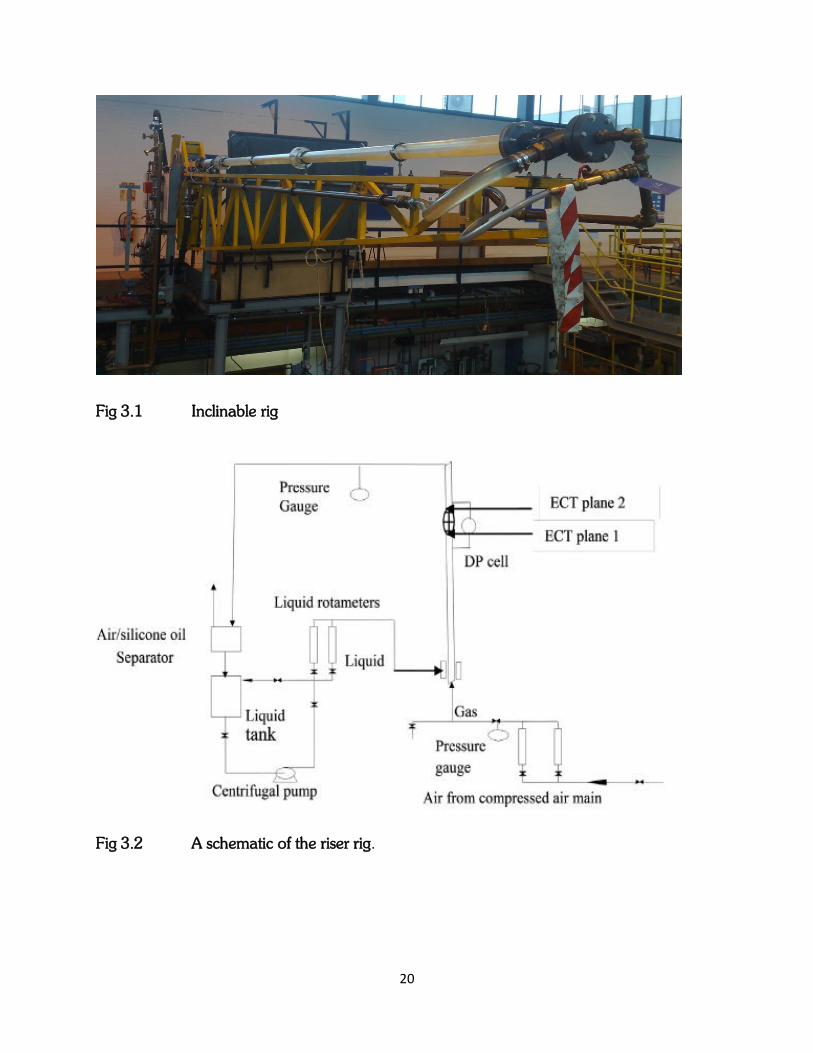
3.2 The experimental facility

The experimental work was carried out on an inclinable pipe flow rig within the Chemical

Engineering Laboratory of University of Nottingham. Figs 3.1 and 3.2 show the

experimental facility. The details of the experiment can be found in Abdulkadir et.al (2014)

20

Fig 3.1 Inclinable rig

Fig 3.2 A schematic of the riser rig.

21

3.3 Determination of characterisation parameters for this present study

In this present work the method of determination of characterisation parameters presented

by Abdulkadir et al. (2014) is adopted.

3.3.1 Translational or rise velocity of Taylor bubble (structure velocity)

Fundamentally translational velocity is given by t

LU N

(2.17)

Where ∆L= the distance between the two ECT planes and ∆t = time taken for the

individual slugs to travel between the two planes.

3.3.1.1 Determination of the distance (∆L) between the two ECT planes

The planes are located at 4.4 m and 4.489 m above the mixer section at the base of the

riser. mmmL 089.04.4489.4

3.3.1.2 Determination of time delay

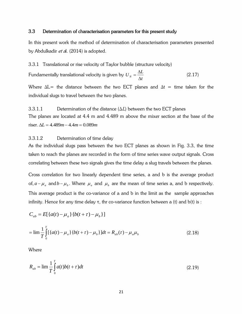
As the individual slugs pass between the two ECT planes as shown in Fig. 3.3, the time

taken to reach the planes are recorded in the form of time series wave output signals. Cross

correlating between these two signals gives the time delay a slug travels between the planes.

Cross correlation for two linearly dependent time series, a and b is the average product

of, aa and bb . Where a and b are the mean of time series a, and b respectively.

This average product is the co-variance of a and b in the limit as the sample approaches

infinity. Hence for any time delay τ, thr co-variance function between a (t) and b(t) is :

}])(}{)([{ baab tbtaEC

baab

T

ba RdttbtaT

)(}])(}{)([{1

lim0

(2.18)

Where

T

ab dttbtaT

R0

)()(1

lim (2.19)

22

The correlation co-efficient is defined as follows

))()0((

)(

)0()0(

)()(

22

bbbaaa

baab

bbaa

abab

RR

R

CC

C

(2.20)

These equations have been pogrammed as computational macro programme to determine

the structure velocity of the liquid slug body, (Abdul-kadir et al. 2014).

Fig 3.3 Void fraction time series from the two ECT probes

3.3.2. Slug frequency

This is the number of slugs passing through a defined pipe cross-section in a given time

period. The power spectral density approach (PSD) defined by Bendat and Piersol (1980)

was used. PSD basically measures how the power in a signal changes over frequency. It is

defined mathematically as the Fourier transform of an auto-correlation sequence. The PSD

function is defined as follows

deRfS fj

abab

2)()( (2.21)

23

3.3.3 Length of the slug unit, the Taylor bubble and the liquid slug

From the relation SU

N

LU where SUL is the length of slug unit, is the time for a

particular slug to pass the probe. But frequency f

1

Therefore f

UL N

SU (2.22)

The length of slug unit is therefore calculated from eq. (2.22)

Again for an individual slug unit, assuming steady state so that the front and back of the slug

have the same velocity

SUiSUi ktL (2.23)

TBiNiTBi tUL (2.24)

SiNiSi tUL (2.25)

Dividing eq. (2.24) by eq. (2.25) results in the following expression

ckt

kt

L

L

Si

TBi

Si

TBi (2.26)

SiTBi cLL (2.27)

But

SiTBiSUi LLL (2.28)

Finally, substituting eq. (2.27) into eq. (2.28) and re-arranging results in the following

expressions

1

c

LL SUi

Si (2.29)

SiSUiTBi LLL (2.30)

24

The lengths of the liquid slug and the Taylor bubble are estimated from eq. (2.29) and eq.

(2.30) respectively

25

CHAPTER 4

RESULTS AND DISCUSSIONS

4.1 Flow pattern of the regime under study

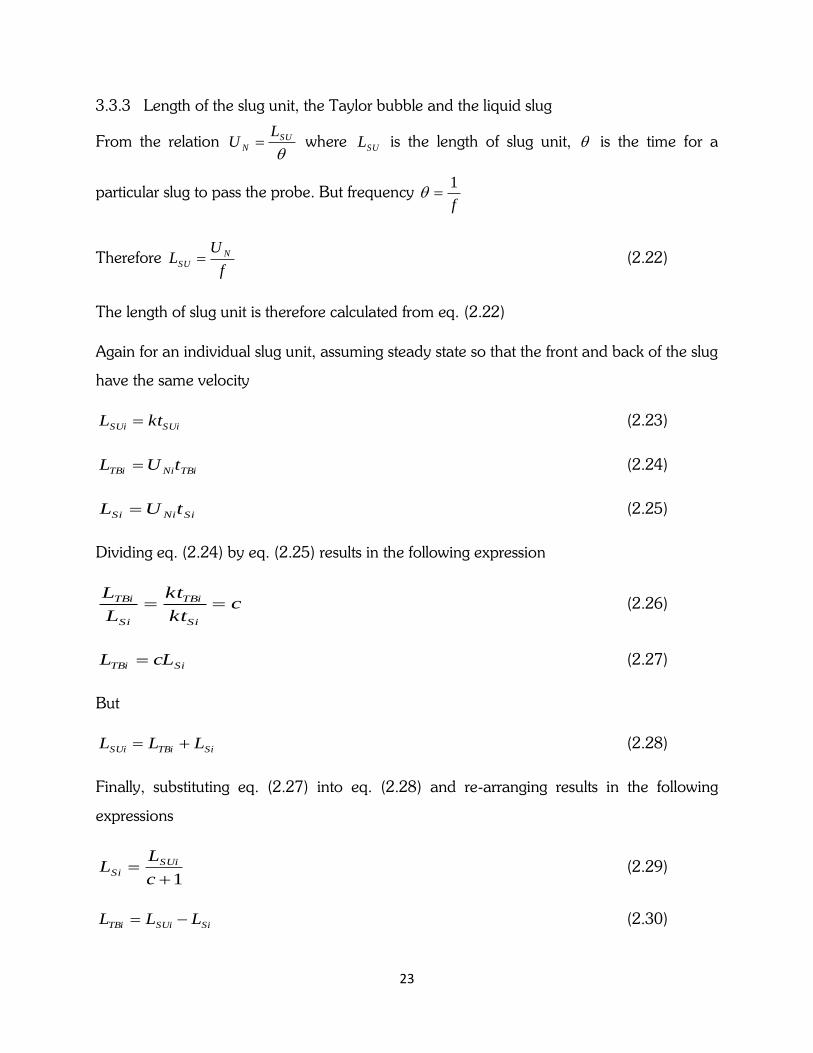
According to Costigan and Whalley (1997) a twin peaked probability density function of the

void fraction measured in the experimental study is a finger print of slug flow as shown in

Fig 4.11. The void fraction in the liquid slug and that in the Taylor bubble are the void

fraction at low and high void fractions respectively. The PDF (Probability Density Function)

shows the dominant void fraction under each flow condition. It was determined by dividing

the total number of data points by dividing the total number of data points in bins width of

0.01 by the sum of the total number of data points.

Fig 4.1 PDF of void fraction showing the signature of slug flow as from experiments

using air-silicone oil as the working fluid.

26

4.2 Structure velocity of Taylor bubble

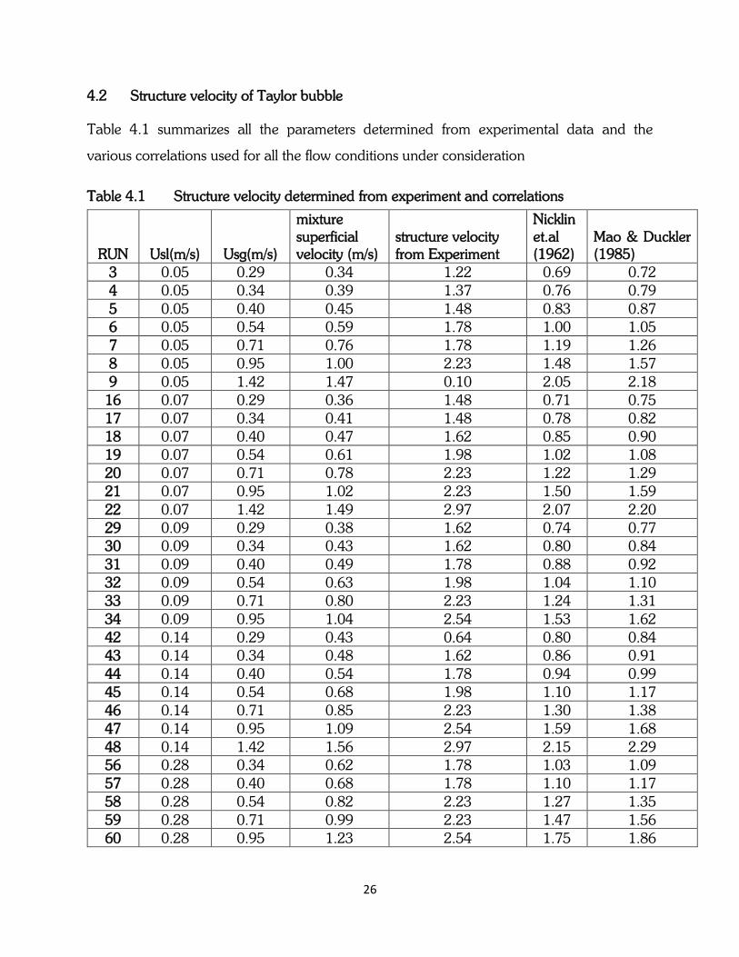
Table 4.1 summarizes all the parameters determined from experimental data and the

various correlations used for all the flow conditions under consideration

Table 4.1 Structure velocity determined from experiment and correlations

RUN Usl(m/s) Usg(m/s)

mixture superficial velocity (m/s)

structure velocity from Experiment

Nicklin et.al (1962)

Mao & Duckler (1985)

3 0.05 0.29 0.34 1.22 0.69 0.72

4 0.05 0.34 0.39 1.37 0.76 0.79

5 0.05 0.40 0.45 1.48 0.83 0.87 6 0.05 0.54 0.59 1.78 1.00 1.05

7 0.05 0.71 0.76 1.78 1.19 1.26

8 0.05 0.95 1.00 2.23 1.48 1.57

9 0.05 1.42 1.47 0.10 2.05 2.18

16 0.07 0.29 0.36 1.48 0.71 0.75

17 0.07 0.34 0.41 1.48 0.78 0.82 18 0.07 0.40 0.47 1.62 0.85 0.90

19 0.07 0.54 0.61 1.98 1.02 1.08

20 0.07 0.71 0.78 2.23 1.22 1.29

21 0.07 0.95 1.02 2.23 1.50 1.59

22 0.07 1.42 1.49 2.97 2.07 2.20

29 0.09 0.29 0.38 1.62 0.74 0.77 30 0.09 0.34 0.43 1.62 0.80 0.84

31 0.09 0.40 0.49 1.78 0.88 0.92

32 0.09 0.54 0.63 1.98 1.04 1.10

33 0.09 0.71 0.80 2.23 1.24 1.31

34 0.09 0.95 1.04 2.54 1.53 1.62

42 0.14 0.29 0.43 0.64 0.80 0.84 43 0.14 0.34 0.48 1.62 0.86 0.91

44 0.14 0.40 0.54 1.78 0.94 0.99

45 0.14 0.54 0.68 1.98 1.10 1.17

46 0.14 0.71 0.85 2.23 1.30 1.38

47 0.14 0.95 1.09 2.54 1.59 1.68

48 0.14 1.42 1.56 2.97 2.15 2.29 56 0.28 0.34 0.62 1.78 1.03 1.09

57 0.28 0.40 0.68 1.78 1.10 1.17

58 0.28 0.54 0.82 2.23 1.27 1.35

59 0.28 0.71 0.99 2.23 1.47 1.56

60 0.28 0.95 1.23 2.54 1.75 1.86

27

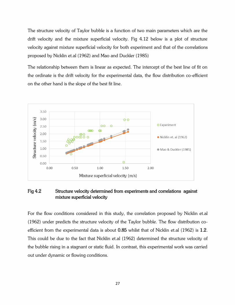
The structure velocity of Taylor bubble is a function of two main parameters which are the

drift velocity and the mixture superficial velocity. Fig 4.12 below is a plot of structure

velocity against mixture superficial velocity for both experiment and that of the correlations

proposed by Nicklin et.al (1962) and Mao and Duckler (1985)

The relationship between them is linear as expected. The intercept of the best line of fit on

the ordinate is the drift velocity for the experimental data, the flow distribution co-efficient

on the other hand is the slope of the best fit line.

Fig 4.2 Structure velocity determined from experiments and correlations against

mixture superficial velocity

For the flow conditions considered in this study, the correlation proposed by Nicklin et.al

(1962) under predicts the structure velocity of the Taylor bubble. The flow distribution co-

efficient from the experimental data is about 0.85 whilst that of Nicklin et.al (1962) is 1.2.

This could be due to the fact that Nicklin et.al (1962) determined the structure velocity of

the bubble rising in a stagnant or static fluid. In contrast, this experimental work was carried

out under dynamic or flowing conditions.

28

The drift velocity obtained according to Nicklin et.al (1962) from Fig 4.12 is about 0.28 as

opposed to that of this experiment which is about 1.24. The difference is because Nicklin

et.al (1962) conducted their study under potential flow where they considered surface

tension and viscosity effects to be negligible and therefore were ignored in the study.

The results obtained from the predictions of Mao and Duckler (1985) just as Nicklin et.al

(1962) under predicts the experimental results. Their prediction is closer to the experimental

result than that of Nicklin et.al (1962). They considered in their study, the influence of the

bubbles in the liquid slug ahead of the Taylor bubble front. They explained that the front of

the Taylor bubble is aerated, and coalescence takes place between the small bubbles and

the Taylor bubbles as the Taylor bubbles move through them at a higher velocity. This

explains why the structural velocity predicted by Mao and Duckler (1985) is higher than that

predicted by Nicklin et.al (1962)

Mao and Duckler (1985) just as Nicklin et.al (1962) also assumed that the effect of surface

tension and viscosity is negligible in the determination of drift velocity.

The observations made have a good level of agreement to that reported much later by

Abdulkadir et.al (2014)

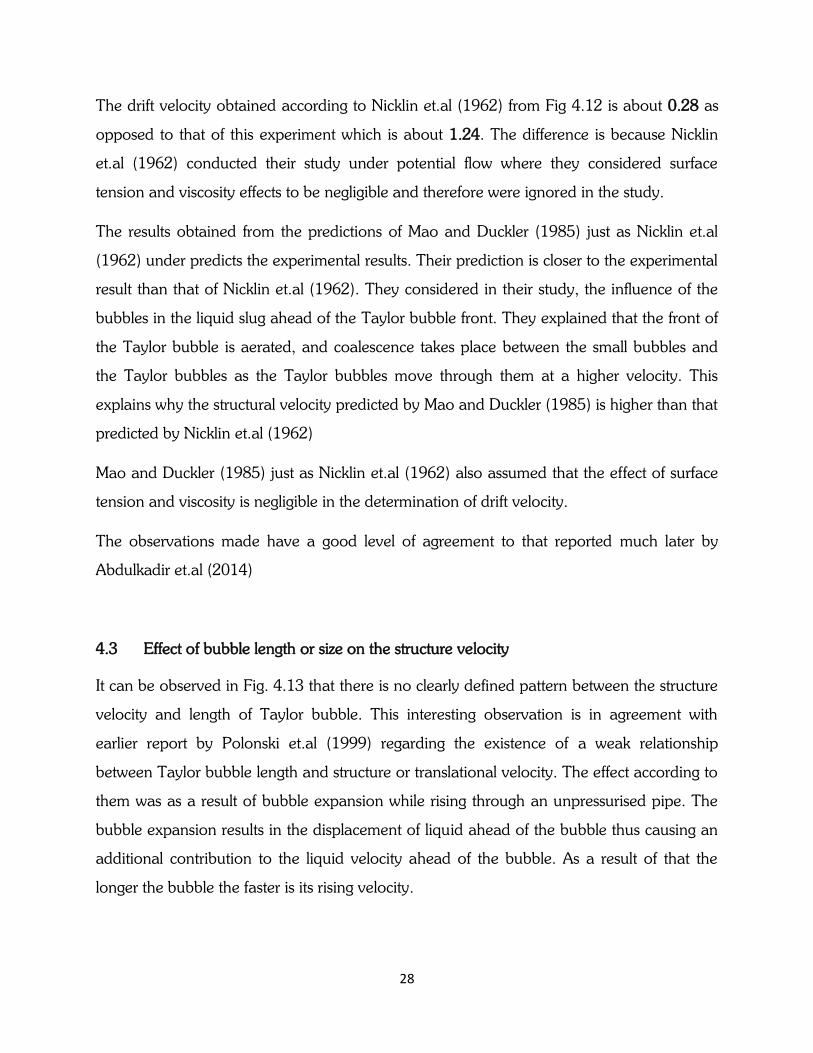
4.3 Effect of bubble length or size on the structure velocity

It can be observed in Fig. 4.13 that there is no clearly defined pattern between the structure

velocity and length of Taylor bubble. This interesting observation is in agreement with

earlier report by Polonski et.al (1999) regarding the existence of a weak relationship

between Taylor bubble length and structure or translational velocity. The effect according to

them was as a result of bubble expansion while rising through an unpressurised pipe. The

bubble expansion results in the displacement of liquid ahead of the bubble thus causing an

additional contribution to the liquid velocity ahead of the bubble. As a result of that the

longer the bubble the faster is its rising velocity.

29

Fig 4.3 Effect of Taylor bubble length on structure velocity

4.4 Void fraction in liquid slug and Taylor bubble.

Table 4.2 is a summary of the various void fractions determined from experiment and

correlations for the flow conditions under study

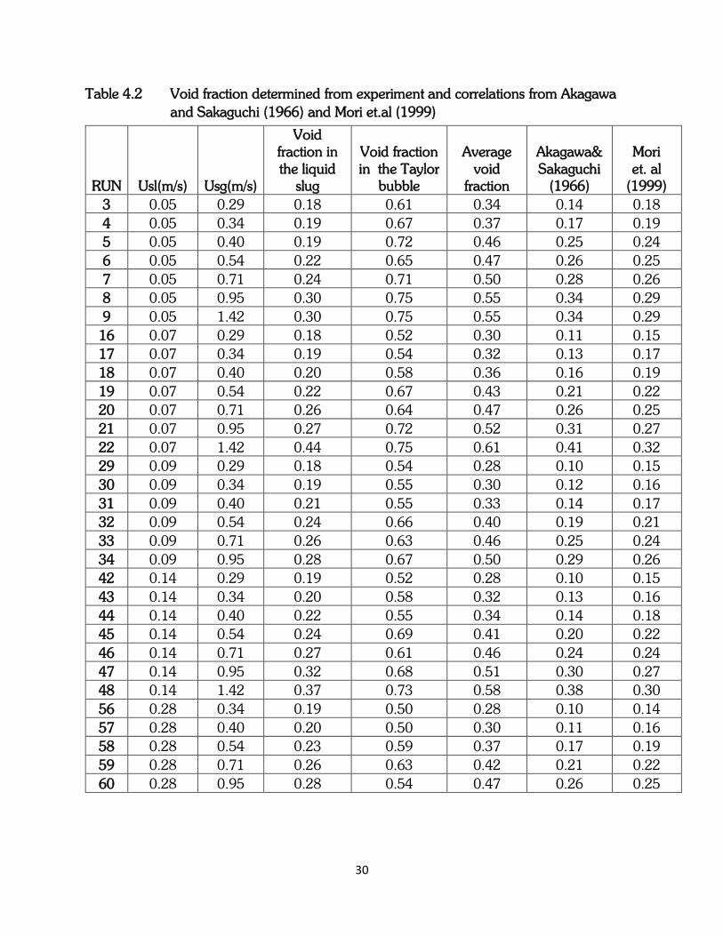
30

Table 4.2 Void fraction determined from experiment and correlations from Akagawa

and Sakaguchi (1966) and Mori et.al (1999)


Void fraction in the liquid

slug

Void fraction in the Taylor

bubble

Average void

fraction

Akagawa& Sakaguchi

(1966)

Mori et. al

(1999)

3 0.05 0.29 0.18 0.61 0.34 0.14 0.18

4 0.05 0.34 0.19 0.67 0.37 0.17 0.19

5 0.05 0.40 0.19 0.72 0.46 0.25 0.24

6 0.05 0.54 0.22 0.65 0.47 0.26 0.25

7 0.05 0.71 0.24 0.71 0.50 0.28 0.26

8 0.05 0.95 0.30 0.75 0.55 0.34 0.29

9 0.05 1.42 0.30 0.75 0.55 0.34 0.29

16 0.07 0.29 0.18 0.52 0.30 0.11 0.15

17 0.07 0.34 0.19 0.54 0.32 0.13 0.17

18 0.07 0.40 0.20 0.58 0.36 0.16 0.19

19 0.07 0.54 0.22 0.67 0.43 0.21 0.22

20 0.07 0.71 0.26 0.64 0.47 0.26 0.25

21 0.07 0.95 0.27 0.72 0.52 0.31 0.27

22 0.07 1.42 0.44 0.75 0.61 0.41 0.32

29 0.09 0.29 0.18 0.54 0.28 0.10 0.15

30 0.09 0.34 0.19 0.55 0.30 0.12 0.16

31 0.09 0.40 0.21 0.55 0.33 0.14 0.17

32 0.09 0.54 0.24 0.66 0.40 0.19 0.21

33 0.09 0.71 0.26 0.63 0.46 0.25 0.24

34 0.09 0.95 0.28 0.67 0.50 0.29 0.26

42 0.14 0.29 0.19 0.52 0.28 0.10 0.15

43 0.14 0.34 0.20 0.58 0.32 0.13 0.16

44 0.14 0.40 0.22 0.55 0.34 0.14 0.18

45 0.14 0.54 0.24 0.69 0.41 0.20 0.22

46 0.14 0.71 0.27 0.61 0.46 0.24 0.24

47 0.14 0.95 0.32 0.68 0.51 0.30 0.27

48 0.14 1.42 0.37 0.73 0.58 0.38 0.30

56 0.28 0.34 0.19 0.50 0.28 0.10 0.14

57 0.28 0.40 0.20 0.50 0.30 0.11 0.16

58 0.28 0.54 0.23 0.59 0.37 0.17 0.19

59 0.28 0.71 0.26 0.63 0.42 0.21 0.22

60 0.28 0.95 0.28 0.54 0.47 0.26 0.25

31

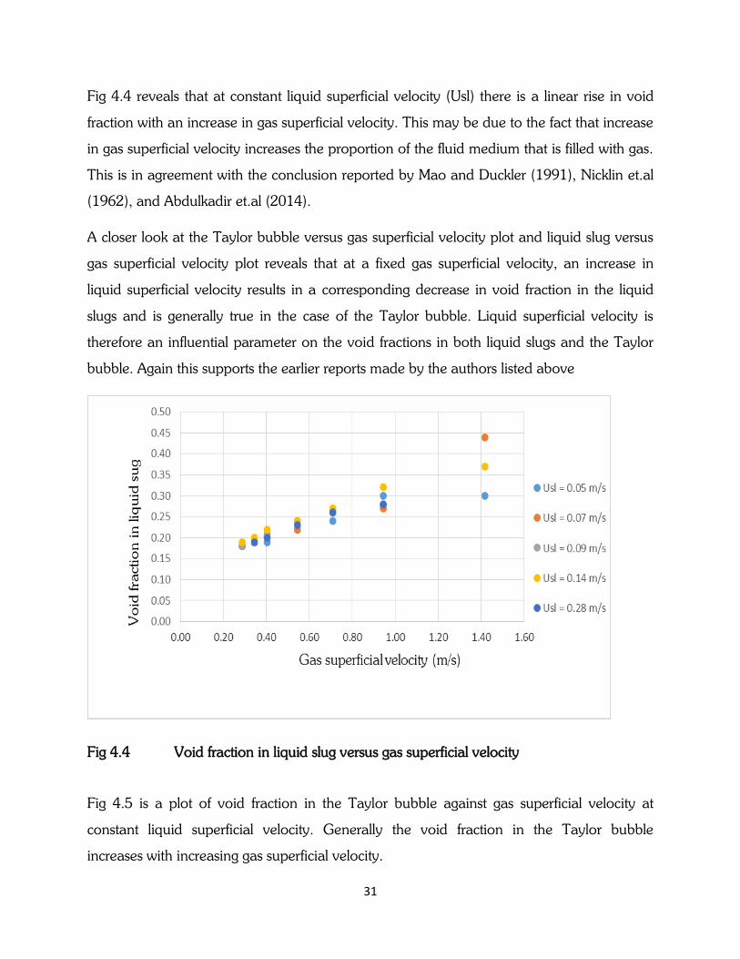
Fig 4.4 reveals that at constant liquid superficial velocity (Usl) there is a linear rise in void

fraction with an increase in gas superficial velocity. This may be due to the fact that increase

in gas superficial velocity increases the proportion of the fluid medium that is filled with gas.

This is in agreement with the conclusion reported by Mao and Duckler (1991), Nicklin et.al

(1962), and Abdulkadir et.al (2014).

A closer look at the Taylor bubble versus gas superficial velocity plot and liquid slug versus

gas superficial velocity plot reveals that at a fixed gas superficial velocity, an increase in

liquid superficial velocity results in a corresponding decrease in void fraction in the liquid

slugs and is generally true in the case of the Taylor bubble. Liquid superficial velocity is

therefore an influential parameter on the void fractions in both liquid slugs and the Taylor

bubble. Again this supports the earlier reports made by the authors listed above

Fig 4.4 Void fraction in liquid slug versus gas superficial velocity

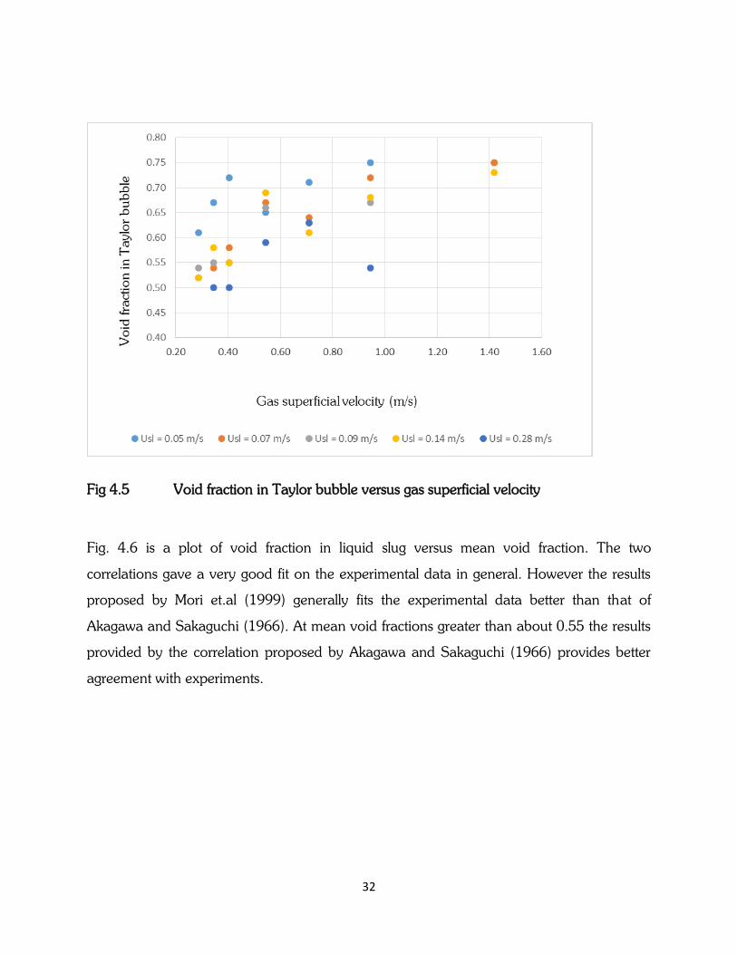
Fig 4.5 is a plot of void fraction in the Taylor bubble against gas superficial velocity at

constant liquid superficial velocity. Generally the void fraction in the Taylor bubble

increases with increasing gas superficial velocity.

32

Fig 4.5 Void fraction in Taylor bubble versus gas superficial velocity

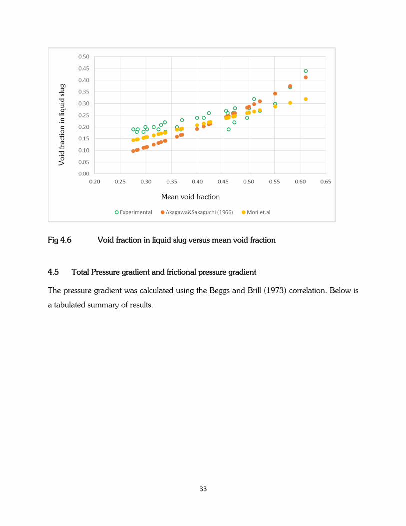
Fig. 4.6 is a plot of void fraction in liquid slug versus mean void fraction. The two

correlations gave a very good fit on the experimental data in general. However the results

proposed by Mori et.al (1999) generally fits the experimental data better than that of

Akagawa and Sakaguchi (1966). At mean void fractions greater than about 0.55 the results

provided by the correlation proposed by Akagawa and Sakaguchi (1966) provides better

agreement with experiments.

33

Fig 4.6 Void fraction in liquid slug versus mean void fraction

4.5 Total Pressure gradient and frictional pressure gradient

The pressure gradient was calculated using the Beggs and Brill (1973) correlation. Below is

a tabulated summary of results.

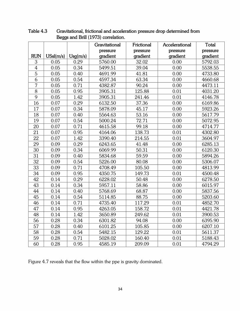
34

Table 4.3 Gravitational, frictional and acceleration pressure drop determined from

Beggs and Brill (1973) correlation.

RUN USsl(m/s) Usg(m/s)

Gravitational pressure gradient

Frictional pressure gradient

Accelerational pressure gradient

Total pressure gradient

3 0.05 0.29 5760.00 32.02 0.00 5792.03 4 0.05 0.34 5499.51 39.04 0.00 5538.55 5 0.05 0.40 4691.99 41.81 0.00 4733.80 6 0.05 0.54 4597.34 63.34 0.00 4660.68 7 0.05 0.71 4382.87 90.24 0.00 4473.11 8 0.05 0.95 3905.31 125.88 0.01 4031.20

9 0.05 1.42 3905.31 241.46 0.01 4146.78 16 0.07 0.29 6132.50 37.36 0.00 6169.86 17 0.07 0.34 5878.09 45.17 0.00 5923.26 18 0.07 0.40 5564.63 53.16 0.00 5617.79 19 0.07 0.54 5000.24 72.71 0.00 5072.95 20 0.07 0.71 4615.58 99.18 0.00 4714.77 21 0.07 0.95 4164.06 138.73 0.01 4302.80 22 0.07 1.42 3390.40 214.55 0.01 3604.97 29 0.09 0.29 6243.65 41.48 0.00 6285.13 30 0.09 0.34 6069.99 50.31 0.00 6120.30 31 0.09 0.40 5834.68 59.59 0.00 5894.26 32 0.09 0.54 5226.00 80.08 0.00 5306.07

33 0.09 0.71 4708.49 105.50 0.00 4813.99 34 0.09 0.95 4350.75 149.73 0.01 4500.48 42 0.14 0.29 6228.02 50.48 0.00 6278.50 43 0.14 0.34 5957.11 58.86 0.00 6015.97 44 0.14 0.40 5768.69 68.87 0.00 5837.56 45 0.14 0.54 5114.85 88.75 0.00 5203.60 46 0.14 0.71 4735.40 117.29 0.01 4852.70 47 0.14 0.95 4263.05 158.72 0.01 4421.78 48 0.14 1.42 3650.89 249.62 0.01 3900.53 56 0.28 0.34 6301.82 94.08 0.00 6395.90 57 0.28 0.40 6101.25 105.85 0.00 6207.10 58 0.28 0.54 5482.15 129.22 0.01 5611.37 59 0.28 0.71 5028.02 160.40 0.01 5188.43 60 0.28 0.95 4585.19 209.09 0.01 4794.29

Figure 4.7 reveals that the flow within the ppe is gravity dominated.

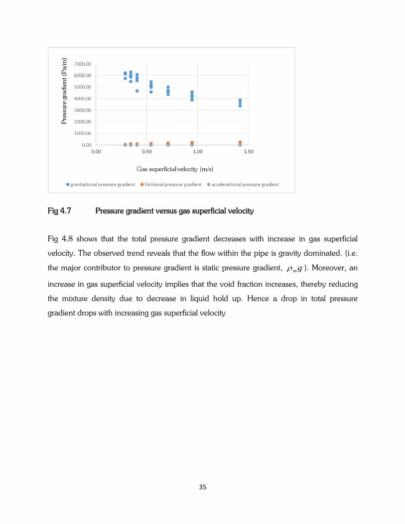
35

Fig 4.7 Pressure gradient versus gas superficial velocity

Fig 4.8 shows that the total pressure gradient decreases with increase in gas superficial

velocity. The observed trend reveals that the flow within the pipe is gravity dominated. (i.e.

the major contributor to pressure gradient is static pressure gradient, gm ). Moreover, an

increase in gas superficial velocity implies that the void fraction increases, thereby reducing

the mixture density due to decrease in liquid hold up. Hence a drop in total pressure

gradient drops with increasing gas superficial velocity

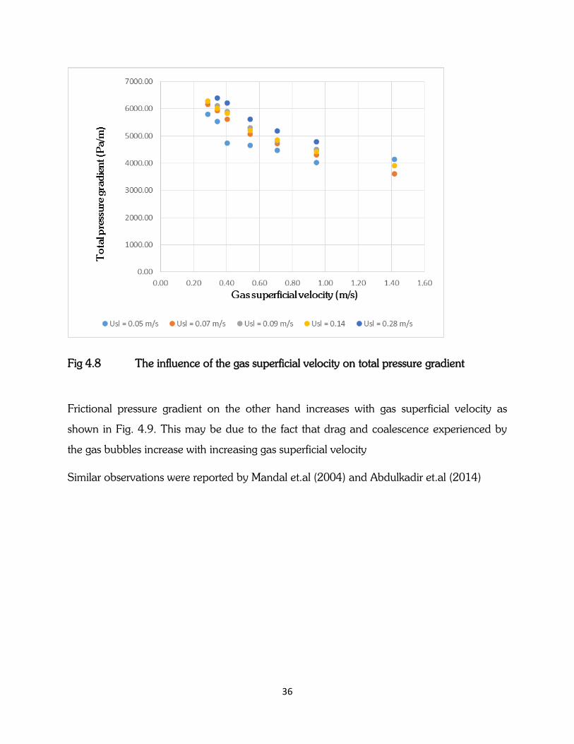
36

Fig 4.8 The influence of the gas superficial velocity on total pressure gradient

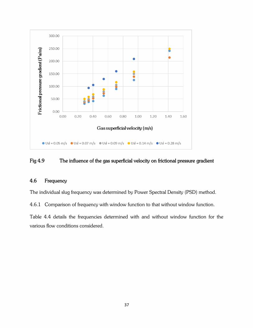
Frictional pressure gradient on the other hand increases with gas superficial velocity as

shown in Fig. 4.9. This may be due to the fact that drag and coalescence experienced by

the gas bubbles increase with increasing gas superficial velocity

Similar observations were reported by Mandal et.al (2004) and Abdulkadir et.al (2014)

37

Fig 4.9 The influence of the gas superficial velocity on frictional pressure gradient

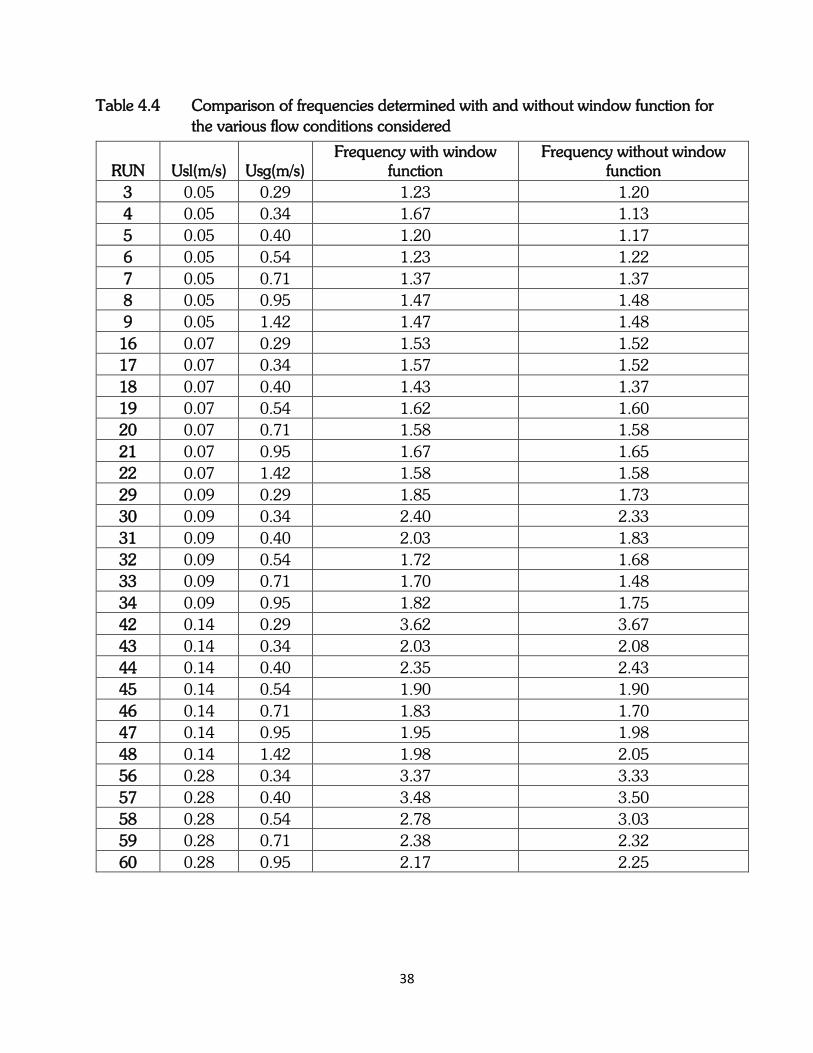
4.6 Frequency

The individual slug frequency was determined by Power Spectral Density (PSD) method.

4.6.1 Comparison of frequency with window function to that without window function.

Table 4.4 details the frequencies determined with and without window function for the

various flow conditions considered.

38

Table 4.4 Comparison of frequencies determined with and without window function for

the various flow conditions considered

RUN Usl(m/s) Usg(m/s) Frequency with window

function Frequency without window

function

3 0.05 0.29 1.23 1.20

4 0.05 0.34 1.67 1.13

5 0.05 0.40 1.20 1.17

6 0.05 0.54 1.23 1.22

7 0.05 0.71 1.37 1.37

8 0.05 0.95 1.47 1.48

9 0.05 1.42 1.47 1.48

16 0.07 0.29 1.53 1.52

17 0.07 0.34 1.57 1.52

18 0.07 0.40 1.43 1.37

19 0.07 0.54 1.62 1.60

20 0.07 0.71 1.58 1.58

21 0.07 0.95 1.67 1.65

22 0.07 1.42 1.58 1.58

29 0.09 0.29 1.85 1.73

30 0.09 0.34 2.40 2.33

31 0.09 0.40 2.03 1.83

32 0.09 0.54 1.72 1.68

33 0.09 0.71 1.70 1.48

34 0.09 0.95 1.82 1.75

42 0.14 0.29 3.62 3.67

43 0.14 0.34 2.03 2.08

44 0.14 0.40 2.35 2.43

45 0.14 0.54 1.90 1.90

46 0.14 0.71 1.83 1.70

47 0.14 0.95 1.95 1.98

48 0.14 1.42 1.98 2.05

56 0.28 0.34 3.37 3.33

57 0.28 0.40 3.48 3.50

58 0.28 0.54 2.78 3.03

59 0.28 0.71 2.38 2.32

60 0.28 0.95 2.17 2.25

39

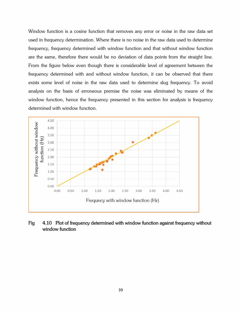
Window function is a cosine function that removes any error or noise in the raw data set

used in frequency determination. Where there is no noise in the raw data used to determine

frequency, frequency determined with window function and that without window function

are the same, therefore there would be no deviation of data points from the straight line.

From the figure below even though there is considerable level of agreement between the

frequency determined with and without window function, it can be observed that there

exists some level of noise in the raw data used to determine slug frequency. To avoid

analysis on the basis of erroneous premise the noise was eliminated by means of the

window function, hence the frequency presented in this section for analysis is frequency

determined with window function.

Fig 4.10 Plot of frequency determined with window function against frequency without

window function

40

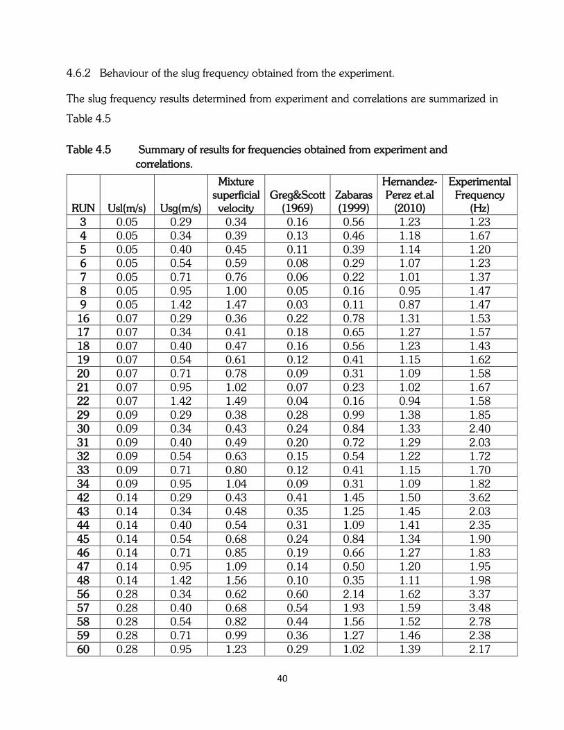
4.6.2 Behaviour of the slug frequency obtained from the experiment.

The slug frequency results determined from experiment and correlations are summarized in

Table 4.5

Table 4.5 Summary of results for frequencies obtained from experiment and

correlations.


Mixture superficial velocity

Greg&Scott (1969)

Zabaras (1999)

Hernandez-Perez et.al

(2010)

Experimental Frequency

(Hz) 3 0.05 0.29 0.34 0.16 0.56 1.23 1.23 4 0.05 0.34 0.39 0.13 0.46 1.18 1.67 5 0.05 0.40 0.45 0.11 0.39 1.14 1.20 6 0.05 0.54 0.59 0.08 0.29 1.07 1.23 7 0.05 0.71 0.76 0.06 0.22 1.01 1.37 8 0.05 0.95 1.00 0.05 0.16 0.95 1.47 9 0.05 1.42 1.47 0.03 0.11 0.87 1.47

16 0.07 0.29 0.36 0.22 0.78 1.31 1.53 17 0.07 0.34 0.41 0.18 0.65 1.27 1.57 18 0.07 0.40 0.47 0.16 0.56 1.23 1.43 19 0.07 0.54 0.61 0.12 0.41 1.15 1.62 20 0.07 0.71 0.78 0.09 0.31 1.09 1.58

21 0.07 0.95 1.02 0.07 0.23 1.02 1.67 22 0.07 1.42 1.49 0.04 0.16 0.94 1.58 29 0.09 0.29 0.38 0.28 0.99 1.38 1.85 30 0.09 0.34 0.43 0.24 0.84 1.33 2.40 31 0.09 0.40 0.49 0.20 0.72 1.29 2.03 32 0.09 0.54 0.63 0.15 0.54 1.22 1.72

33 0.09 0.71 0.80 0.12 0.41 1.15 1.70 34 0.09 0.95 1.04 0.09 0.31 1.09 1.82 42 0.14 0.29 0.43 0.41 1.45 1.50 3.62 43 0.14 0.34 0.48 0.35 1.25 1.45 2.03 44 0.14 0.40 0.54 0.31 1.09 1.41 2.35

45 0.14 0.54 0.68 0.24 0.84 1.34 1.90 46 0.14 0.71 0.85 0.19 0.66 1.27 1.83 47 0.14 0.95 1.09 0.14 0.50 1.20 1.95 48 0.14 1.42 1.56 0.10 0.35 1.11 1.98 56 0.28 0.34 0.62 0.60 2.14 1.62 3.37 57 0.28 0.40 0.68 0.54 1.93 1.59 3.48 58 0.28 0.54 0.82 0.44 1.56 1.52 2.78 59 0.28 0.71 0.99 0.36 1.27 1.46 2.38 60 0.28 0.95 1.23 0.29 1.02 1.39 2.17

41

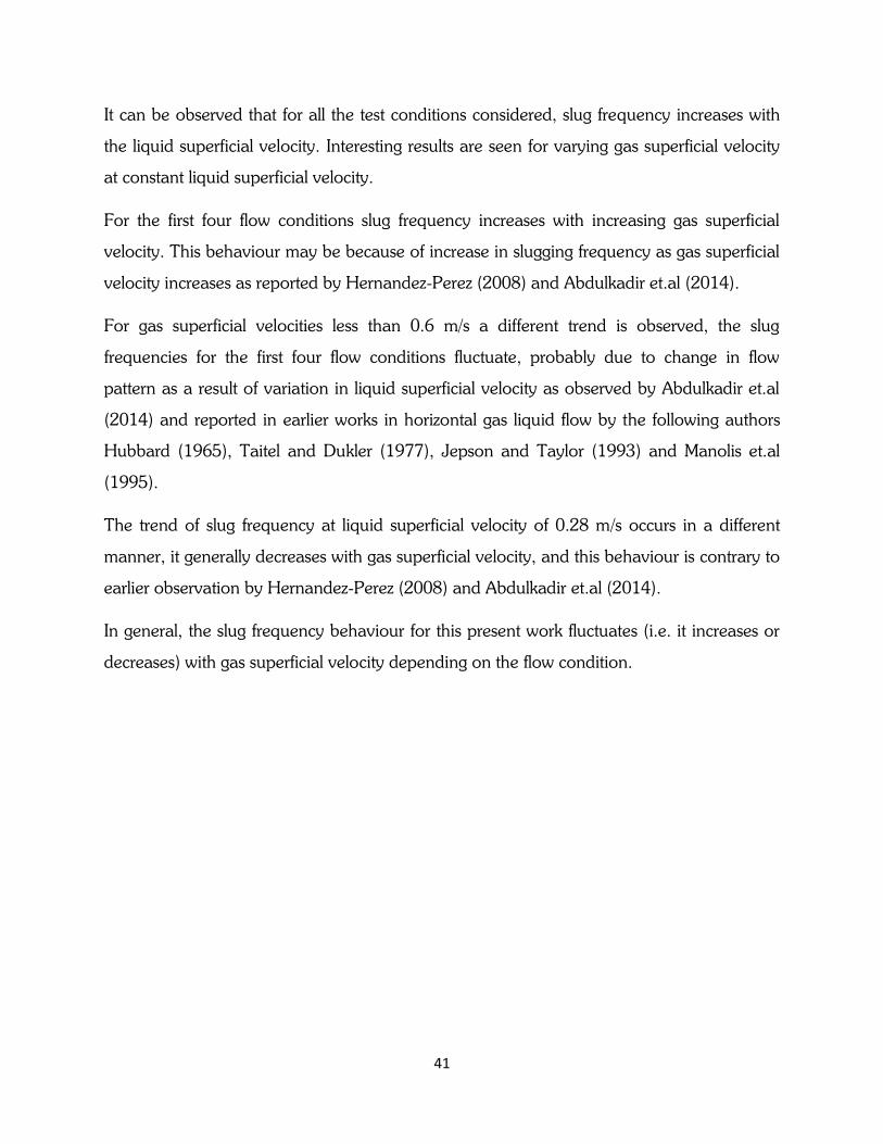
It can be observed that for all the test conditions considered, slug frequency increases with

the liquid superficial velocity. Interesting results are seen for varying gas superficial velocity

at constant liquid superficial velocity.

For the first four flow conditions slug frequency increases with increasing gas superficial

velocity. This behaviour may be because of increase in slugging frequency as gas superficial

velocity increases as reported by Hernandez-Perez (2008) and Abdulkadir et.al (2014).

For gas superficial velocities less than 0.6 m/s a different trend is observed, the slug

frequencies for the first four flow conditions fluctuate, probably due to change in flow

pattern as a result of variation in liquid superficial velocity as observed by Abdulkadir et.al

(2014) and reported in earlier works in horizontal gas liquid flow by the following authors

Hubbard (1965), Taitel and Dukler (1977), Jepson and Taylor (1993) and Manolis et.al

(1995).

The trend of slug frequency at liquid superficial velocity of 0.28 m/s occurs in a different

manner, it generally decreases with gas superficial velocity, and this behaviour is contrary to

earlier observation by Hernandez-Perez (2008) and Abdulkadir et.al (2014).

In general, the slug frequency behaviour for this present work fluctuates (i.e. it increases or

decreases) with gas superficial velocity depending on the flow condition.

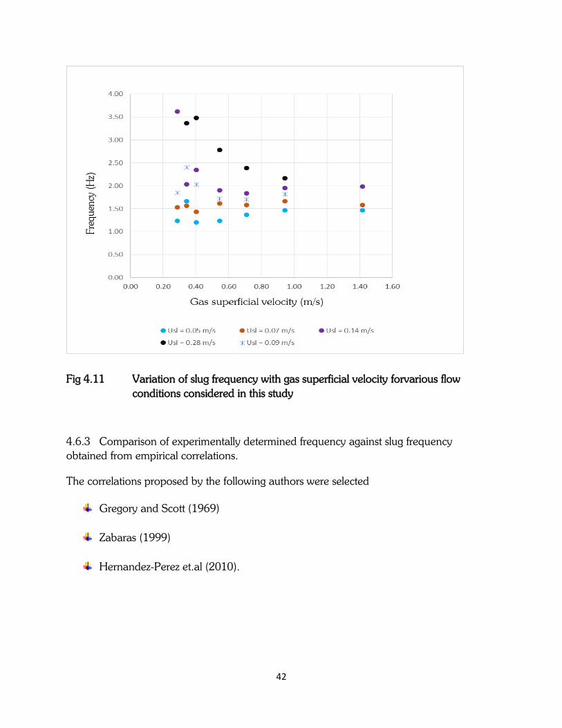
42

Fig 4.11 Variation of slug frequency with gas superficial velocity forvarious flow

conditions considered in this study

4.6.3 Comparison of experimentally determined frequency against slug frequency

obtained from empirical correlations.

The correlations proposed by the following authors were selected

Gregory and Scott (1969)

Zabaras (1999)

Hernandez-Perez et.al (2010).

43

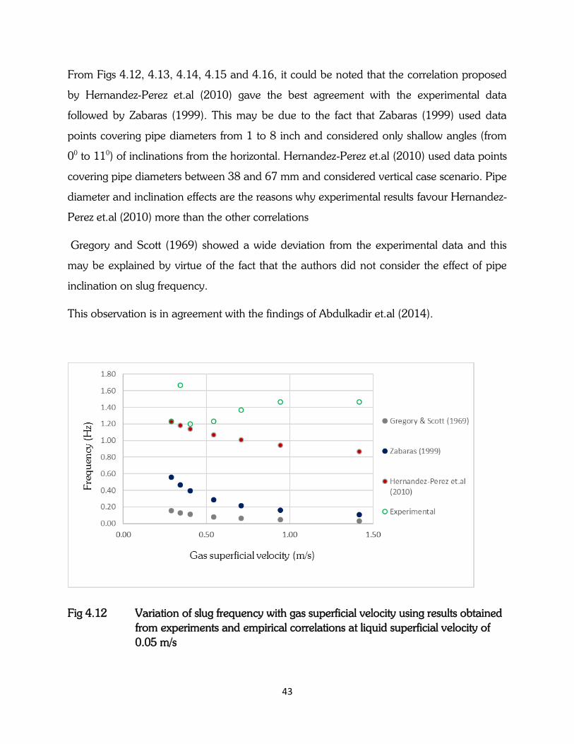
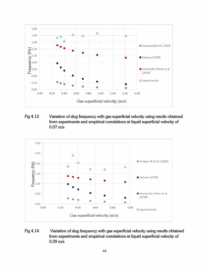
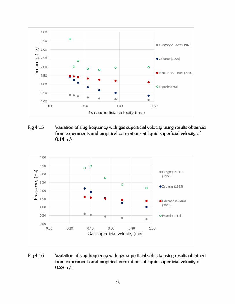
From Figs 4.12, 4.13, 4.14, 4.15 and 4.16, it could be noted that the correlation proposed

by Hernandez-Perez et.al (2010) gave the best agreement with the experimental data

followed by Zabaras (1999). This may be due to the fact that Zabaras (1999) used data

points covering pipe diameters from 1 to 8 inch and considered only shallow angles (from

00 to 110) of inclinations from the horizontal. Hernandez-Perez et.al (2010) used data points

covering pipe diameters between 38 and 67 mm and considered vertical case scenario. Pipe

diameter and inclination effects are the reasons why experimental results favour Hernandez-

Perez et.al (2010) more than the other correlations

Gregory and Scott (1969) showed a wide deviation from the experimental data and this

may be explained by virtue of the fact that the authors did not consider the effect of pipe

inclination on slug frequency.

This observation is in agreement with the findings of Abdulkadir et.al (2014).


from experiments and empirical correlations at liquid superficial velocity of

0.05 m/s

44



0.07 m/s



0.09 m/s

45



0.14 m/s



0.28 m/s

46

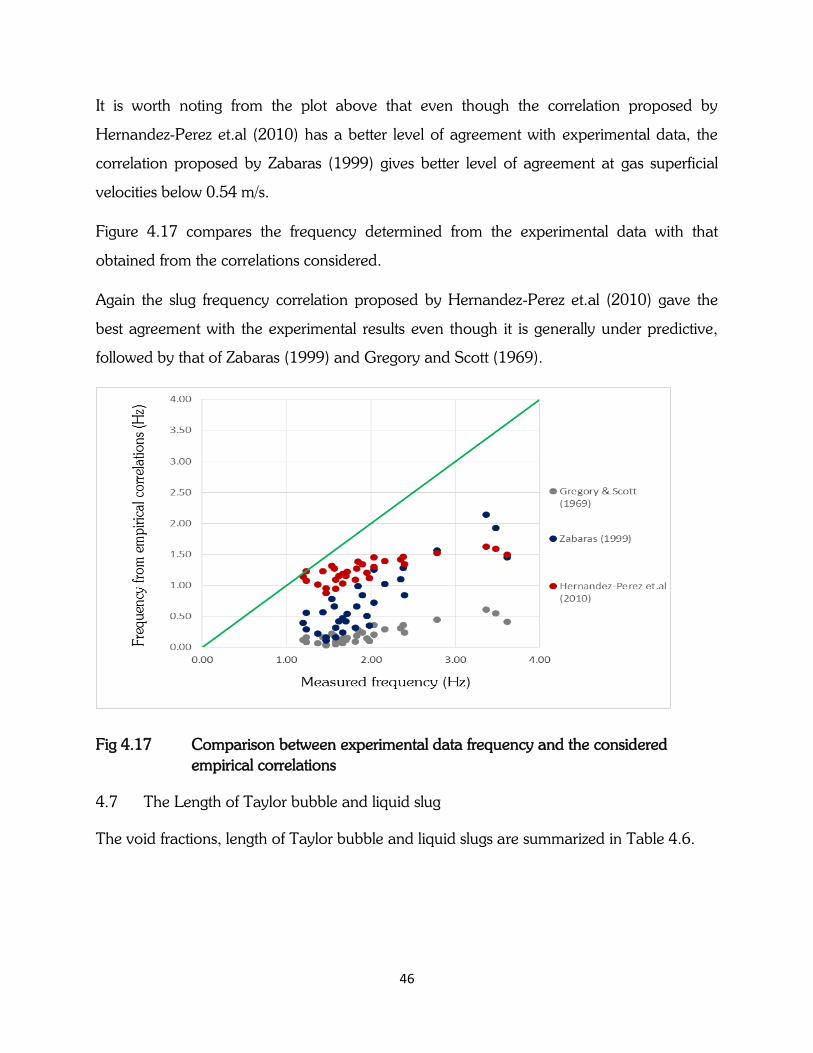
It is worth noting from the plot above that even though the correlation proposed by

Hernandez-Perez et.al (2010) has a better level of agreement with experimental data, the

correlation proposed by Zabaras (1999) gives better level of agreement at gas superficial

velocities below 0.54 m/s.

Figure 4.17 compares the frequency determined from the experimental data with that

obtained from the correlations considered.

Again the slug frequency correlation proposed by Hernandez-Perez et.al (2010) gave the

best agreement with the experimental results even though it is generally under predictive,

followed by that of Zabaras (1999) and Gregory and Scott (1969).

Fig 4.17 Comparison between experimental data frequency and the considered

empirical correlations

4.7 The Length of Taylor bubble and liquid slug

The void fractions, length of Taylor bubble and liquid slugs are summarized in Table 4.6.

47

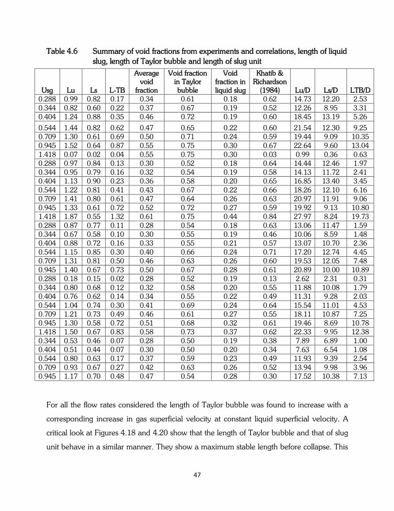
Table 4.6 Summary of void fractions from experiments and correlations, length of liquid

slug, length of Taylor bubble and length of slug unit

Usg Lu Ls L-TB

Average void

fraction

Void fraction in Taylor bubble

Void fraction in liquid slug

Khatib & Richardson

(1984) Lu/D Ls/D LTB/D 0.288 0.99 0.82 0.17 0.34 0.61 0.18 0.62 14.73 12.20 2.53 0.344 0.82 0.60 0.22 0.37 0.67 0.19 0.52 12.26 8.95 3.31 0.404 1.24 0.88 0.35 0.46 0.72 0.19 0.60 18.45 13.19 5.26

0.544 1.44 0.82 0.62 0.47 0.65 0.22 0.60 21.54 12.30 9.25 0.709 1.30 0.61 0.69 0.50 0.71 0.24 0.59 19.44 9.09 10.35 0.945 1.52 0.64 0.87 0.55 0.75 0.30 0.67 22.64 9.60 13.04 1.418 0.07 0.02 0.04 0.55 0.75 0.30 0.03 0.99 0.36 0.63 0.288 0.97 0.84 0.13 0.30 0.52 0.18 0.64 14.44 12.46 1.97 0.344 0.95 0.79 0.16 0.32 0.54 0.19 0.58 14.13 11.72 2.41 0.404 1.13 0.90 0.23 0.36 0.58 0.20 0.65 16.85 13.40 3.45 0.544 1.22 0.81 0.41 0.43 0.67 0.22 0.66 18.26 12.10 6.16 0.709 1.41 0.80 0.61 0.47 0.64 0.26 0.63 20.97 11.91 9.06

0.945 1.33 0.61 0.72 0.52 0.72 0.27 0.59 19.92 9.13 10.80 1.418 1.87 0.55 1.32 0.61 0.75 0.44 0.84 27.97 8.24 19.73 0.288 0.87 0.77 0.11 0.28 0.54 0.18 0.63 13.06 11.47 1.59 0.344 0.67 0.58 0.10 0.30 0.55 0.19 0.46 10.06 8.59 1.48 0.404 0.88 0.72 0.16 0.33 0.55 0.21 0.57 13.07 10.70 2.36 0.544 1.15 0.85 0.30 0.40 0.66 0.24 0.71 17.20 12.74 4.45 0.709 1.31 0.81 0.50 0.46 0.63 0.26 0.60 19.53 12.05 7.48

0.945 1.40 0.67 0.73 0.50 0.67 0.28 0.61 20.89 10.00 10.89 0.288 0.18 0.15 0.02 0.28 0.52 0.19 0.13 2.62 2.31 0.31 0.344 0.80 0.68 0.12 0.32 0.58 0.20 0.55 11.88 10.08 1.79 0.404 0.76 0.62 0.14 0.34 0.55 0.22 0.49 11.31 9.28 2.03

0.544 1.04 0.74 0.30 0.41 0.69 0.24 0.64 15.54 11.01 4.53 0.709 1.21 0.73 0.49 0.46 0.61 0.27 0.55 18.11 10.87 7.25 0.945 1.30 0.58 0.72 0.51 0.68 0.32 0.61 19.46 8.69 10.78 1.418 1.50 0.67 0.83 0.58 0.73 0.37 0.62 22.33 9.95 12.38

0.344 0.53 0.46 0.07 0.28 0.50 0.19 0.38 7.89 6.89 1.00 0.404 0.51 0.44 0.07 0.30 0.50 0.20 0.34 7.63 6.54 1.08 0.544 0.80 0.63 0.17 0.37 0.59 0.23 0.49 11.93 9.39 2.54 0.709 0.93 0.67 0.27 0.42 0.63 0.26 0.52 13.94 9.98 3.96 0.945 1.17 0.70 0.48 0.47 0.54 0.28 0.30 17.52 10.38 7.13

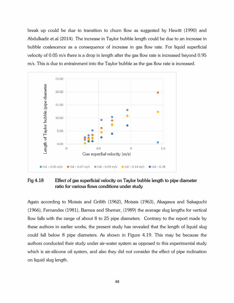
For all the flow rates considered the length of Taylor bubble was found to increase with a

corresponding increase in gas superficial velocity at constant liquid superficial velocity. A

critical look at Figures 4.18 and 4.20 show that the length of Taylor bubble and that of slug

unit behave in a similar manner. They show a maximum stable length before collapse. This

48

break up could be due to transition to churn flow as suggested by Hewitt (1990) and

Abdulkadir et.al (2014). The increase in Taylor bubble length could be due to an increase in

bubble coalescence as a consequence of increase in gas flow rate. For liquid superficial

velocity of 0.05 m/s there is a drop in length after the gas flow rate is increased beyond 0.95

m/s. This is due to entrainment into the Taylor bubble as the gas flow rate is increased.

Fig 4.18 Effect of gas superficial velocity on Taylor bubble length to pipe diameter

ratio for various flows conditions under study

Again according to Moissis and Grifith (1962), Moissis (1963), Akagawa and Sakaguchi

(1966), Fernandes (1981), Barnea and Shemer, (1989) the average slug lengths for vertical

flow falls with the range of about 8 to 25 pipe diameters. Contrary to the report made by

these authors in earlier works, the present study has revealed that the length of liquid slug

could fall below 8 pipe diameters. As shown in Figure 4.19. This may be because the

authors conducted their study under air-water system as opposed to this experimental study

which is air-silicone oil system, and also they did not consider the effect of pipe inclination

on liquid slug length.

49

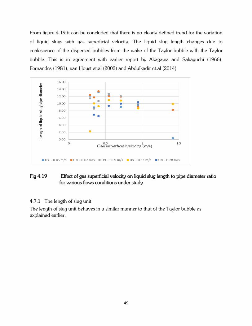
From figure 4.19 it can be concluded that there is no clearly defined trend for the variation

of liquid slugs with gas superficial velocity. The liquid slug length changes due to

coalescence of the dispersed bubbles from the wake of the Taylor bubble with the Taylor

bubble. This is in agreement with earlier report by Akagawa and Sakaguchi (1966),

Fernandes (1981), van Houst et.al (2002) and Abdulkadir et.al (2014)

Fig 4.19 Effect of gas superficial velocity on liquid slug length to pipe diameter ratio

for various flows conditions under study

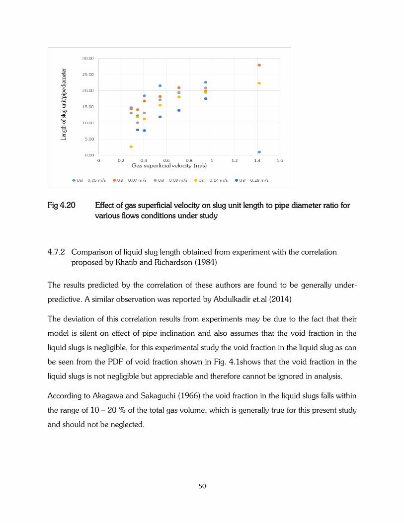
4.7.1 The length of slug unit

The length of slug unit behaves in a similar manner to that of the Taylor bubble as

explained earlier.

50

Fig 4.20 Effect of gas superficial velocity on slug unit length to pipe diameter ratio for

various flows conditions under study

4.7.2 Comparison of liquid slug length obtained from experiment with the correlation

proposed by Khatib and Richardson (1984)

The results predicted by the correlation of these authors are found to be generally under-

predictive. A similar observation was reported by Abdulkadir et.al (2014)

The deviation of this correlation results from experiments may be due to the fact that their

model is silent on effect of pipe inclination and also assumes that the void fraction in the

liquid slugs is negligible, for this experimental study the void fraction in the liquid slug as can

be seen from the PDF of void fraction shown in Fig. 4.1shows that the void fraction in the

liquid slugs is not negligible but appreciable and therefore cannot be ignored in analysis.

According to Akagawa and Sakaguchi (1966) the void fraction in the liquid slugs falls within

the range of 10 – 20 % of the total gas volume, which is generally true for this present study

and should not be neglected.

51

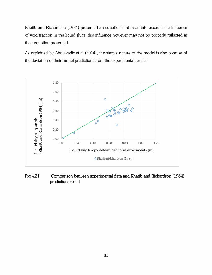
Khatib and Richardson (1984) presented an equation that takes into account the influence

of void fraction in the liquid slugs, this influence however may not be properly reflected in

their equation presented.

As explained by Abdulkadir et.al (2014), the simple nature of the model is also a cause of

the deviation of their model predictions from the experimental results.

Fig 4.21 Comparison between experimental data and Khatib and Richardson (1984)

predictions results

52

CHAPTER 5

CONCLUSIONS AND RECOMMENDATIONS

5.1 Conclusions

The study produced experimental results to characterize slug flow within an 80 degree

inclination pipe when certain known amounts of air and silicone oil are introduced at the

base of the riser. The flow characteristics were obtained using electrical capacitance

tomography data. Below are the conclusions arrived at:

a) A linear relationship was obtained between structure velocity and mixture superficial

velocity. This is in agreement with earlier report by (Abdulkadir et.al 2014). The

linear relationship confirms the empirical correlations proposed by Nicklin et.al

(1962) and Mao and Duckler (1985). The correlation proposed by Mao and Dukler

(1985) gave better level of agreement with the experimental data

b) Drift velocity from experimental results (air-silicone oil system) is higher than that

obtained from the correlations proposed by Nicklin (1962) and Mao and Duckler

(1985) which was for air-water system. The deviation of the drift velocities produced

by these correlations from experiments could be attributed to the fact that surface

tension and viscosity effects were neglected. Surface tension and viscosity are

therefore important parameters to be considered in drift velocity analysis since they

are not always negligible.

c) A quite weak relationship was obtained between the length of Taylor bubble and the

structure velocity of the Taylor bubble. This is in good agreement with earlier report

by Polonski et.al (1999) regarding the effect of Taylor bubble length on structure

velocity of the Taylor bubble

d) The total pressure gradient was found to decrease with increasing gas superficial

velocity whiles the frictional pressure gradient was found to increase.

53

e) At a fixed liquid superficial velocity increase in gas superficial velocity results in an

increase in the void fraction in both the Taylor bubble and the liquid slug. Also at

fixed gas superficial velocity increase in liquid superficial velocity was found to result

in a decrease in void fraction in the liquid slugs and is generally true in the case of

the Taylor bubble. Liquid superficial velocity is therefore an influential parameter on

the void fraction in liquid slug and Taylor bubble. These findings agree well with

earlier published works and more recently Abdulkadir et al (2014)

f) A comparison of experimental data of void fraction in liquid slugs with the empirical

correlations proposed by Akagawa and Sakaguchi (1966) and Mori et.al (1999)

showed a very good agreement. The relationship prosed by Mori et.al (1999) gave

better agreement in general but at mean void fractions greater than 0.55 the

relationship proposed by Akagawa and Sakaguchi (1996) is more reliable

g) Frequency of slugs fluctuates with gas superficial velocity, they increase and decrease

depending on the flow condition. A comparison of experimental results with the

correlations proposed by Gregory and Scott (1969), Zabaras (1999) and Hernandez-

Perez et.al (2010) reveals that the correlation proposed by Hernandez-Perez et.al

(2010) gives the best level of agreement with experimental data.

h) The length of Taylor bubble and slug unit were found to increase with increasing gas

superficial velocity. The liquid slug length fluctuates due to coalescence of the

dispersed bubbles from the wake of the Taylor bubble with the Taylor bubble. This is

in agreement with earlier report by Akagawa and Sakaguchi (1966), Fernandes

(1981), van Houst et.al (2002) and Abdulkadir et.al (2014)

i) The results provided by Khatib and Richardson (1984) method for determining liquid

slug length yielded fairly good agreement with experimental data.

j) Comparing the findings of this present work (which is for 800 pipe inclination) to that

of earlier work by Abdulkadir et.al (2014) (which is for 900 pipe inclination) reveals

good agreement in almost all the observations made in the hydrodynamic behaviour

54

of the slug flow characterisation parameters. Pipe inclination therefore did not have

much effect on the slug flow behaviour.

5.2 Recommendations

Future work should study the hydrodynamic behaviour of slug flow in 800 pipe

inclined from the horizontal using wire mesh sensor (WMS) and the obtained results

should be compared to those obtained for the same pipe inclination.

Pressure drop for this work was determined from correlation due to absence of

pressure drop data for the pipe inclination under study. It is recommended that

pressure drop test be run and compared with the pressure drop results in this present

work to serve as a verification.

Future work should consider investigating the hydrodynamic slug flow in pipes of

higher angles of deviation from the vertical and establish if any, the point at which

the slug flow characteristics change.

55

References:

Abdulkadir, M. (2014), ‘‘Experimental study of the hydrodynamic behaviour of slug flow in a

vertical riser’’, Chemical Engineering Science, Vol. 106, No. 0009-2509, pp. 60-75.

Ahmed, W.H. (2011), ‘‘Experimental Investigation of air-oil slug flow using capacitance probes,

hot-film anemometer, and image processing’’, International Journal of Multiphase

Flow, Vol. 37, pp. 876-887.

Ahmad, W.R., DeJesus, J.M., Kawaji, M., 1998. Falling film hydrodynamics in slug flow. Chem.

Eng. Sci. 53, 123-130

Akagawa, K. Sakaguchi, T. (1966) Fluctuation of void fraction in two phase flow (2 nd report,

analysis of flow configurations considering the existence of small bubbles in liquid

slugs), Bull. JSME, 104-110

Alves, I.N., Shoham, O., Taitel, Y., 1993. Drift velocity of elongated bubbles in inclined pipes.

Chem. Eng. Sci. 48, 3063-3070.

Barnea, D. and Brauner, N. (1985), Hold-up for liquid slugs in two phase intermittent flow, Int.

J. of multiphase flow, 11, 43-49

Barnea, D. and Shemer, L. (1989), void fraction measurements in vertical slug flow:

applications to slug characteristics and transition, Int. J. of Multiphase flow, 15,

495-504.

Barnea, D. and Taitel, Y. (1993), A model for slug length distribution in gas-liquid slug flow, Int.

J. of Multiphase flow, Vol 19. No. 5, pp. 828-838.

Bendiksen, K., 1984. An experimental investigation of the motion of long bubbles in inclined

tubes. Int. J. Multiphase Flow 10, 467-483

Bendiksen, K., 1985. On the motion of long bubbles in vertical tubes. Int. J. Multiphase Flow

11, 797-812.

Benjamin, T.B., 1968. Gravity currents and related phenomena. J. Fluid Mech. 21, 209-248

56

Bernicot. M. and Drouffe, J.M. (1989), slug length distribution in two-phase transportation

systems. In Proc. 4th Int. Conf. Multi-phase flow, Nice. France, pp.485-493. BHRA,

Cranfield, Beds.

Brill, J.P. Schmidt. Z., Coberly, W.A., Herrin, J.D. and Moore, D.W. (1981), Analysisof two

phase tests in large diameter flow lines in Prudhoe Bay field, SPE J, 271, 363-378.

Bugg, J.D., Mack, K., Rezkallah, K.S., 1998. A numerical model of Taylor bubbles rising through

stagnant liquid in vertical tubes. Int. J. Multiphase Flow 24, 271-281.

Bonnecaze, R.H., Eriskine Jr., W., Greskovich, E.J., 1971. Holdup and pressure drop for two-

phase slug flow in inclined pipelines. AIChE J. 17, 1109-1113.

Cai,J.Y.Wang, H.W., Hong, T. and Jepson, W.P.,(1999), Slug frequency and length inclined

large diameter multiphase pipe line, Multiphase flow and heat transfer, proceedings

of fourth international symposium, Xi’an, China, 195-202.

Collins, R., de Moraes, F.F., Davidson, J.F., Harrison, D., 1978. The motion of a large gas

bubble rising through liquid flowing in a tube. J. Fluid Mech. 89, 497-514.

Clarke, A., Issa, R.I., 1992. A multidimensional computational model of slug flow. In: AIChE

Annual Spring Meeting, New Orleans.

Clarke, A., Issa, R.I., 1993. A multidimensional computational model of slug flow. Gas-Liquid

Flows '93 FED-165,119-130

Clift, R, Grace, J.R., Weber, M.E., (1978). Bubbles, Drops and Particles. Academic Press, NY

Davies, R.M., Taylor, G.I., (1950). The mechanics of large bubbles rising through extended

liquids and through liquid in tubes. Proc. R. Soc. London 200, 375-390.

DeJesus, J.D., Ahmad, W., Kawaji, M., 1995. Experimental study of flow structure in vertical slug

flow. In: Proc. 2nd Int. Conf. Multiphase Flow, Kyoto, P9-51, P9-55

Dhulesia, H. Bernicot, M. and Deheuvels, P. (1991), Statistical analysis and modelling of slug

lengths,In Proc. 5th Int. Conf. on Multiphase production, Cannes, France, pp. 80-

112, BHRA Cranfield, Beds.

Donevski, B., Saga, T., Kobayashi, T., Segawa, S., 1995. An automatic image analysis of two-

phase bubbly flowregime. In: Proc. 2nd Int. Conf. Multiphase Flow, Kyoto, pp.1-21,

pp. 1-26.

57

Duckler, A.E. Moalem-Maron, D. and Brauner, N. (1985), A physical model for predicting

minimum stable slug length, Chem. Eng. Sci. 40, pp. 1379-1385.

Dumitresku, D.T., (1943). Stromung an einer Luftblase im senkrechten Rohr. Z. Angew. Math.

Mech. 23, 139-149.

Fabre, J. and Line, A. (1992), Modelling of two-phase slug flow, A. Rev. Fluid Mech. 24, 21-46

Fernandes, R.C., Semiat, R., and Dukler, A.E., (1983), ‘‘Hydrodynamics model for gas–liquid

slug flow in vertical tubes’’. AIChE J., Vol. 29, pp. 981–989.

Fernandes, R. C. (1981), Experimental and theoretical studies of isothermal upward gas-liquid

flows in vertical tubes, Ph.D thesis, University of Houston, TX.

Goldsmith, H.L., Mason, S.G., 1962. The movement of single large bubbles in closed vertical

tubes. J. Fluid Mech.14, 52-58

Gregory, G. & Scott, D.S., (1969.) Correlation of liquid slug velocity and frequency in horizontal

co-current slug flow, AICHEJL VoLl5, pp.933-935

Griffith, P., Wallis, G.B., 1959. MIT Technical Report No. 15. NONR-1959, 1841.

Hernandez-Perez, V., AbdulKadir, M., Azzopadi, B.J., (2010), ‘‘Slugging frequency correlation for

inclined gas-liquid flow.’’, World Acad. Sci. Eng. Technol. 61, 44-51

Hubbard, M, (1965) An analysis of horizontal gas-liquid slug flow, Ph.D thesis, University of

Houston,

TX. Hill; TJ. and D.G. Wood, (1990), A new approach to the prediction of slug frequency, SPE

Annual Teehnical Conf, pp.141-149,

Khatib, Z. and Richardson, J.F., (1984), ‘‘vertical co-current flow of air and shear thinning

suspensions of kaolin’’, Chem. Eng. Res. Des. Vol. 62, pp. 139-154.

Kordban, E.S., and Ranov, T.,(1970), Mechanism of slug formation in horizontal two phase flow.

Trans. ASME j. Basic Eng. 92, 857-864.

Kvernvold, O., Vindoy, V., Sontvedt, T., Saasen, A., Selmen-Olsen, S., 1984. Velocity

distribution in horizontal slug flow. Int. J. Multiphase Flow 10, 441-457

58

Lunde, K., Perkins, R.J., 1995. A method for the detailed study of bubble motion and

deformation. In: Proceedings of the 2nd Internat. Conf. on Multiphase Flow, Kyoto,

AV17-AV24.

Nicklin, D.J., Wilkes, J.O., Davidson, J.F., 1962. Two-phase flow in vertical tubes. Trans. Inst.

Chem. Eng. 40, 61-68.

Nickens, H. V. and Yannitell, D. W. 1987 The effects of surface tension and viscosity on the rise

velocity of a large gas bubble in a closed, vertical liquid-filled tube. Int. J. Multiphase

Flow 13, 57-69.

Nydal, O.J. Pintus. S. and Andreussi, P. (1992), statistical characterisation of slug flow in

horizontal pipes, Int. J. of Multiphase flow 18, pp.439-453.

Mao, Z.S., Dukler, A., 1989. An experimental study of gas-liquid slug flow. Experiments in Fluids

8, 169-182.

Mao, Z.S., Dukler, A., 1990. The motion of Taylor bubbles in vertical tubes: I. A numerical

simulation for the shape and rise velocity of Taylor bubbles in stagnant and flowing

liquid. J. Comp. Phys. 91, 132-160

Moissis, R. (1963), The transition from slug to homogeneous two-phase flow, J. of heat transfer,

85, 366-370.

Moissis, R. and Griffith, P. (1962), Entrance effects in two face slug flow, J. of Heat transfer, 85,

366-370.

Mishima K., and Ishii, M., (1980) Theoritical prediction of onset of horizontal slug flow Trans.

ASME j. Fluids Eng. 102, 441-445.

Nakoryakov, V.E., Kashinsky, O.N., Kozmenko, B.K., 1986. Experimental study of gas-liquid

slug flow in a small- diameter vertical pipe. Int. J. Multiphase Flow 12 (3), 337-355.

Nakoryakov, V.E., Kashinsky, O.N., Petukhov, A.V., Gorelik, R.S., 1989. Study of local

hydrodynamic characteristics of upward slug flow. Experiments in Fluids 7, 560-

566

Pinto AMFR, Campos JBLM (1996), Coalescence of two gas slugs rising in vertical colum of

liquid, Chemical Engineering Science, Vol 51, pp 45-54

59

Polonsky, S., Barnea, D., Shemer, L., 1999. Averaged and time-dependent characteristics of the

motion of an elongated bubble in a vertical pipe. Int. J. Multiphase Flow 25, 795-

812

Saether. G., Bendiksen. K. Muller, J. and Froland, E. (1990), The fractal statistics of liquid slugs,

Int. J. of Multi-phase flows 16, pp.1117-1129.

Shemer, L. and Barnea, D. (1987), Visualization of the instantaneous velocity profiles in gas-

liquid slug flows, Physicochem. Hydrodynam. 8, 243-253

Singh, G., Griffith, P., 1970. Determination of the pressure drop optimum pipe size for a two-

phase slug flow in an inclined pipe. J. Eng. Ind. 92, 717-726

Taitel, Y. & Dukler, A.E., (1977), A model for slug frequency during gas •.liquid flow in

horizontal and near horizontal pipes, lnt.J. Multiphase Flow Vo.l.3, pp.585-596.

Taitel, Y. Barnea, D. and Duckler, A. E. (1980), Modelling flow pattern transitions for steady

upward gas-liquid flow in vertical tubes, AICH JI, 26, pp. 345-354.

Tassin, A.L., Nikitopolous, D.E., 1995. Non-intrusive measurements of bubble size and velocity.

Experiments in Fluids 19, 121-132.

Trocconi, E., (1990), Prediction of slug frequency in horizontal two. Phase slug flow; .AlCHE JL

Vo.1.36, pp, 70 1-709,.

Tung, K.W., Parlange, J.Y., 1976. Note on the motion of long bubbles in closed tubes -

influence of surface tension. Acta Mechanica 24, 313-317

Van Hout, R., Shemer, L. and Barnea, D. (1992), spatial distribution of void fraction within the

liquid slug and some other related parameters, Int. J of Multiphase flow 18, 831-

845.

Van Hout, R., Barnea, D. and Shemer, L. (2002), Translational velocities of elongated bubbles

in continuous flow, Int. J of Multiphase flow 28, 1333-1350.

Zabaras, G.J., (2000), prediction of slug frequency for gas/liquid flows, SPE j 5 (3), 252-258.

60

Documents

HYDRODYNAMICS BEHAVIOUR OF SLUG FLOW IN 80 OFF THE