Hydrodynamical Analysis of Bottom-hinged Oscillating

Wave Surge Converters

Inês Furtado Marques Mendes da Cruz Alves

Thesis to obtain the Master of Science Degree in

Mechanical Engineering

Supervisors: Prof. Carlos António Pancada Guedes Soares

Dr. Debabrata Karmakar

Examination Committee

Chairperson: Prof. Mário Manuel Gonçalves da Costa

Supervisor: Prof. Carlos António Pancada Guedes Soares

Member of the Committee: Prof. Luís Manuel de Carvalho Gato

July 2016

ii

DEDICATION

______________________________________________________________

To Paulo Furtado Mendes da Cruz Alves

iii

ACKNOWLEDGMENTS

______________________________________________________________

This work has been performed within the project 0250/1133 financed by the Foundation for

Science and Technology (“Fundação para a Ciência e Tecnologia”) for the Centre for Marine

Technology and Ocean Engineering (CENTEC).

I express my appreciation and gratitude to my supervisors, Prof. Carlos Guedes Soares and

Dr. Debabrata Karmakar, for their guidance and cooperation during the research work and

preparation of this thesis.

I am also grateful to my parents for all the support they have been in my life and for providing

me the opportunity to conclude this entire academic path.

Finally and most importantly, I express my sincere gratitude to my husband Paulo, whose love,

support, motivation and inspiration make everything possible. Above all, I thank him for helping me

becoming a better person each and every day.

iv

ABSTRACT

______________________________________________________________

In the present study, the wave energy conversion of a bottom-hinged, fully submerged

oscillating wave surge converter is analysed.

An optimal wave energy converter maximises the energy capture while reducing the loads

endured by the device structure to the minimum possible. In order to accomplish this design, an

understanding of the hydrodynamics of the device is of foremost importance. Therefore, the goal of

this dissertation is to obtain the necessary insight into the parameters that influence the

performance of an oscillating wave surge converter.

A mathematical model for a single oscillating wave surge converter as part of an infinite in-line

array of devices is presented, assuming it is subjected to the action of regular, monochromatic

incoming waves. Potential fluid flow is also assumed. This mathematical model was implemented in

a MATLAB algorithm which convergence is also studied.

Using this algorithm, hydrodynamical parameters (flap width, spatial period between plates,

flap height, water depth and flap thickness) of the system are computed and their influence over the

power extraction and efficiency of the device is evaluated.

Results show that, in general, the extracted power and capture factor increase with increasing

width, thickness and ratio between the flap height and the water depth at which the device is

located. The most important factor in designing a wave energy converter was found to be the range

of most frequent periods of the incoming waves. To maximise efficiency, the wave energy converter

should be designed and optimised for the most common sea states.

Keywords: Oscillating wave surge converter, wave energy, energy converter, nearshore

resource, ocean engineering

v

RESUMO

______________________________________________________________

Neste trabalho é analisada a conversão de energia das ondas por conversores oscilantes

totalmente submersos, com eixo de rotação ao nível do fundo do mar.

Um conversor de energia otimizado maximiza a energia capturada, minimizando as cargas às

quais a sua estrutura está sujeita. Para que um conversor seja concebido deste modo, é da maior

importância compreender a influência dos parâmetros hidrodinâmicos no seu desempenho, motivo

pelo qual esta dissertação tem por objectivo compreender a influência dos diferentes parâmetros

na eficiência de um conversor oscilante.

É apresentado um modelo matemático para um conversor oscilante como parte de um conjunto

de infinitos conversores dispostos em linha reta, assumindo que é acionado por ondas regulares em

escoamento potencial. Este modelo foi implementado recorrendo a um algoritmo em MATLAB, cuja

convergência é também analisada.

Através deste algoritmo, é estudada a influência de vários parâmetros sobre a potência extraída

e a eficiência. A largura, altura e espessura da placa, a distância entre conversores e a profundidade

à qual estes se encontram são os parâmetros analisados.

Concluiu-se que, de um modo geral, a potência e a eficiência do sistema aumentam à medida que

aumenta a largura da placa, a espessura e a razão entre a altura da placa e a profundidade a que se

encontra. Concluiu-se que o fator mais importante no projeto do tipo de conversor de energia das

ondas estudado é o intervalo dos períodos das ondas incidentes mais frequentes, para os quais o

conversor deve ser projetado e otimizado.

Palavras-chave: Conversor de energia das ondas oscilante, energia das ondas, conversores de

energia, recursos nearshore, engenharia oceânica

vi

TABLE OF CONTENTS

______________________________________________________________

DEDICATION ii

ACKNOWLEDGMENTS iii

ABSTRACT iv

RESUMO v

TABLE OF CONTENTS vi

LIST OF FIGURES vii

LIST OF TABLES ix

NOMENCLATURE AND ABBREVIATIONS x

1 INTRODUCTION 1

1.1 Current Trend and Potential of the Wave Energy Sector 1

1.2 Outline of Dissertation 4

2 OVERVIEW OF WAVE ENERGY DEVICES 6

2.1 Wave Energy Technologies 6

2.1.1 Bottom-hinged oscillating wave surge converters 9

2.1.2 Power Take-Off Systems 11

2.2 Wave Energy Resource 12

2.3 Ocean Waves 14

2.3.1 Governing Equations and Water-Solid Interaction 15

3 NUMERICAL INVESTIGATION OF A SURGING WEC 19

3.1 Analytical Model 19

3.2 Body Motion 22

4 HYDRODYNAMICAL PERFORMANCE OF A SURGING WEC 28

4.2 Numerical Evaluation 28

4.2 Hydrodynamic Coefficients Analysis 32

4.2.1 Flap width, w 33

4.2.2 Spatial period, b 36

4.2.3 Water depth, h, and flap height, hf 38

4.2.4 Water depth, h, and flap height, hf 42

5 CONCLUSIONS AND FUTURE WORK 44

REFERENCES 46

vii

LIST OF FIGURES

______________________________________________________________

Fig. 1-1 - Estimated renewable energy share of global energy production at the end of 2014 [3] 2

Fig. 2-1 - Different classifications of WECs [1] (adapted) 6

Fig. 2-2 - Pelamis Wave Power [9] (adapted) 7

Fig. 2-3 - Terminator [1] (adapted) 7

Fig. 2-4 - Point Absorber [1] (adapted) 7

Fig. 2-5 - Classification of WECs according to working principle 8

Fig. 2-6 – Oyster [10] 9

Fig. 2-7 - Array of WaveRoller devices [4] 9

Fig. 2-8 - Wave overtopping reservoir [1] (adapted) 9

Fig. 2-9 - Bottom-hinged OWSC equipped with a submerged electrical generator [1] (adapted) 10

Fig. 2-10 - PTO classes [2] (adapted) 11

Fig. 2-11 - Surge phenomenon [4] 14

Fig. 2-12 - Geometry of a single flap in the open ocean; a) plan view; b) section [12] (adapted) 16

Fig. 3-1 - Geometry of the in-line array; a) plan view; b) section [18] (adapted) 20

Fig. 4-1 - Convergence of the relative error between every compared length of the integration

interval, L (average of the relative errors for all the period of the incoming waves considered) 31

Fig. 4-2 - Convergence of the relative error between every compared values of m (average of the

relative errors for all the period of the incoming waves considered) 31

Fig. 4-3 - Convergence of the relative error between every the compared values of N and P (average

of the relative errors for all the periods of the incoming waves considered) 32

Fig. 4-4 - Behaviour of the exciting torque for different values of w, as a function of T 34

Fig. 4-5 - Behaviour of the extractable power for different values of w, as a function of T 34

Fig. 4-6 - Behaviour of the capture factor for different values of w, as a function of T 34

Fig. 4-7 - Average CF for different flap widths 36

Fig. 4-8 - Behaviour of the exciting torque for different values of b as a function of T 37

Fig. 4-9 - Behaviour of the exploitable power for different values of b as a function of T 37

Fig. 4-10 - Behaviour of the capture factor for several values of b as a function of T 38

Fig. 4-11 - Behaviour of |F| for different values of h as a function of T for hf = 10 m 39

Fig. 4-12 - Behaviour of P for different values of h as a function of T for hf = 10 m 39

Fig. 4-13 - Behaviour of the exploitable power for different values of h as a function of T (solid line

for hf = 10 m and dashed line for hf = 8 m) 40

Fig. 4-14 - Behaviour of CF for different values of h as a function of T for hf = 10 m 40

viii

Fig. 4-15 - Behaviour of the capture factor for different values of h as a function of T (solid line for

hf = 10 m and dashed line for hf = 8 m) 41

Fig. 4-16 - Behaviour of the extractable power for different ratios of the covered water: 50% (solid

line) and 70% (dashed line) 41

Fig. 4-17 - Behaviour of the capture factor for different ratios of the covered water: 50% (solid line)

and 70% (dashed line) 42

Fig. 4-18 - Behaviour of the extractable power for different values of a as a function of T 43

Fig. 4-19 - Behaviour of the capture factor for different values of a as a function of T 43

ix

LIST OF TABLES

______________________________________________________________

Table 4-1 - Initial parameter set for the convergence and hydrodynamical analyses 28

Table 4-2 - First iteration of the numerical analysis of the length of the integration intervals

(L = 0,1) 29

Table 4-3 - Second iteration of the numerical analysis of the length of the integration Interval

(L = 0,05) 29

Table 4-4 - Relative errors (in %) between the results obtained for L = 0,1 and L = 0,05 30

Table 4-5 - Final parameter set after convergence analysis 32

Table 4-6 - Increase in CF when increasing w from 14 m to 28 m and from 26 m to 30 m 35

x

NOMENCLATURE AND ABBREVIATIONS

______________________________________________________________

Latin Symbols

Symbol Description

A Amplitude scale of the wave field

a Flap thickness

a' Non-dimensional flap thickness

AI Amplitude of the incident waves

AI' Non-dimensional amplitude of the incident waves

b Spatial period

C Hydrostatic coefficient

C' Non-dimensional hydrostatic coefficient

c Height of the bottom foundation

c' Non-dimensional height of the bottom foundation

CF Capture factor

Cg Group velocity of the incident waves

F Complex exciting torque

F’ Non-dimensional complex exciting torque

ℱ External torque applied on the flap

𝑓 External forces applied per unit volume of fluid

g Acceleration due to gravity

h Water depth

h' Non-dimensional water depth

hf Flap height

h'f Non-dimensional flap height

I Moment of inertia of the flap

I’ Non-dimensional moment of inertia of the flap

�⃗⃗� Unitary vector normal to a surface

P Average extractable power over a period

P' Non-dimensional average extractable power over a period

p Fluid pressure

Pe Electrical power

Ph Harvested power

T Period of the incident waves

xi

T’ Non-dimensional period of the incident waves

t Time

t' Non-dimensional time

𝒯 Sum of all the moments applied on the flap

�⃗⃗� Velocity of the pitching flap

�⃗� Velocity of an element of fluid

w Flap width

w’ Non-dimensional flap width

Greek Symbols

Symbol Description

η Function of the surface of the open ocean

θ Angular displacement

θ’ Non-dimensional angular displacement

λ Wavelength

μ Added torque due to inertia

μ’ Non-dimensional added torque due to inertia

ν Radiation damping

ν' Non-dimensional radiation damping

νk Kinematic viscosity coefficient

νpto Damping of the power take-off system

ν’pto Non-dimensional damping of the power take-off system

ρf Density of the flap

ρ Density of the ocean water

Φ Velocity potential

Φ' Non-dimensional velocity potential

ω Frequency of the incoming waves

ω’ Non-dimensional frequency of the incoming waves

Acronyms and Abbreviations

Symbol Description

OWSC Oscillating wave surge converter

PTO Power take-off

RES Renewable energy sources

WEC Wave energy converter

WET Wave energy technology

1

1CHAPTER 1

INTRODUCTION ______________________________________________________________

Depletion of fossil fuels, global warming and the need of improving energy security by exploiting

indigenous resources have raised environmental awareness and the need and urgency of increasing

the contribution of renewable sources in energy production.

Renewable energy sources (RES) are being largely developed in order to replace fossil fuels.

Wave energy represents a huge resource, largely unexploited. Unlike other renewable sources of

energy, it is not yet well developed and there is no unique leading technology to exploit this

resource.

The potential of wave energy is vast and has stimulated the interest of many countries that

could employ wave energy as a secure and reliable source of electricity in the future.

In order to make wave energy technologies (WET) economically viable, it is necessary to study

the parameters which influence their performance and find the best parameter set. To achieve this

goal regarding oscillating wave surge converters (OWSC), this thesis describes an hydrodynamic

analysis of a bottom-hinged flap in which is studied the influence of several parameters in the

performance of this type of wave energy converters (WEC), using an semi-analytical approach by

implementing a MATLAB algorithm.

1.1 Current Trend and Potential of the Wave Energy Sector

Ocean energy is a term encompassing all of the renewable energy resources found in oceans and

seas, which use the kinetic, potential, chemical or thermal properties of seawater. These can be

harvested in many forms: by exploiting the tidal range, the tidal currents, the energy contained in

surface waves, the ocean currents or the thermal and salinity gradients in the water. Ocean energy

devices convert the different forms of energy contained in the water into more useful forms,

typically electricity, but other uses are also possible, such as water desalinisation, cooling or air

compressed supply for aquaculture [1]. More particularly, WECs transform kinetic and potential

energy of ocean surface waves into another form of energy.

Of all the forms of energy comprised in ocean energy, tidal range, tidal stream and wave energy

converters are the most advanced technologies. In Europe, wave energy is the ocean energy

resource with the highest deployment potential, being its potential far superior than that of tidal

energy [1,2].

As environmental awareness and the need of energetic independence increase, more and more

attention is drawn to renewable sources of energy. Although patents for renewable energy

2

technologies exist for more than a century, serious academic interest began in the 1970s with the

oil crisis and since then many concepts of WEC have been patented and developed, providing a

wide variety of designs and applications [1,2].

The employment of renewable energies in electricity production has been growing in the last

decades due to its several advantages. It is one of the most important steps towards the

decarbonisation of industry in general and electricity industry in particular. For countries that

include renewable sources in their energy mix, i.e. in the range of energy sources contributing to

the final energy consumption, it is an assurance of energy independence, not only because they

become less dependent on fossil fuel producers, but also because combining different renewable

sources of energy improves overlapping of energy supplies, leading to a decrease of variability of

resources, improving reliability and consequently contributing to energy security.

Due to benefits of RES and the need of replacing non-renewable sources, international interest

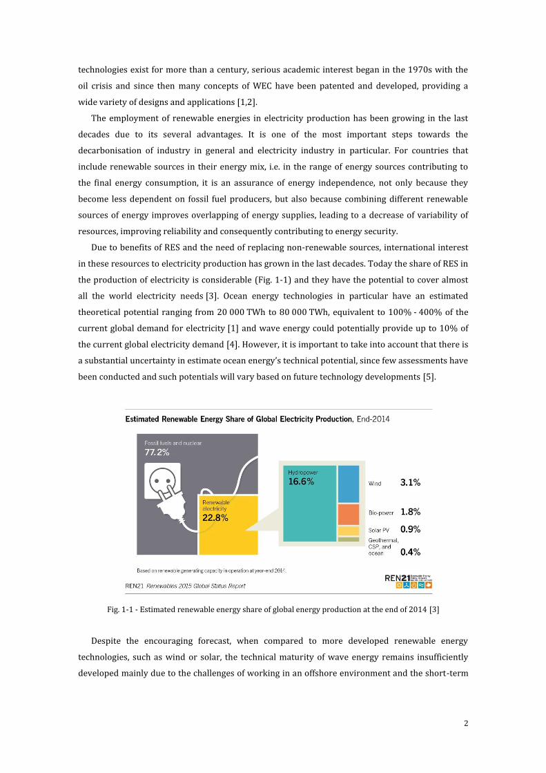
in these resources to electricity production has grown in the last decades. Today the share of RES in

the production of electricity is considerable (Fig. 1-1) and they have the potential to cover almost

all the world electricity needs [3]. Ocean energy technologies in particular have an estimated

theoretical potential ranging from 20 000 TWh to 80 000 TWh, equivalent to 100% - 400% of the

current global demand for electricity [1] and wave energy could potentially provide up to 10% of

the current global electricity demand [4]. However, it is important to take into account that there is

a substantial uncertainty in estimate ocean energy’s technical potential, since few assessments have

been conducted and such potentials will vary based on future technology developments [5].

Fig. 1-1 - Estimated renewable energy share of global energy production at the end of 2014 [3]

Despite the encouraging forecast, when compared to more developed renewable energy

technologies, such as wind or solar, the technical maturity of wave energy remains insufficiently

developed mainly due to the challenges of working in an offshore environment and the short-term

3

outlook for this sector is still very modest, since these technologies experience challenges, such as

technical, environmental or financial barriers.

Since WET is still in its early stages of development, only in the last years full-scale prototypes

have been built and deployed. These prototypes must be developed, tested and optimised so WETs

become cost competitive and technologically reliable before entering the electricity market and

complement or provide an alternative to other RES. Currently, many wave energy companies are at

an advanced stage of technological development with technologies nearing pre-commercial

demonstration and others deploying full-scale prototypes in real-sea environments, with the

purpose of deploying utility scale arrays in the next decade. Nevertheless, only a small amount of

devices has sustained harsh and energetic sea states and endured long operational hours, such as

Oyster and Pelamis, for example. So far, most of the wave energy deployments have consisted in

single-machine prototype testing and some of the existing WETs are already progressing toward

the installation of device arrays [1,2].

Among the different forms of ocean energy, wave and tidal stream are the ocean energy

technologies that have attracted the most commercial interest, considering their geographical

availability and level of technological maturity and these are the forms of ocean energy which are

expected to contribute the most to the European energy system in the next decades [1].

In Europe, several sites can be found where the deployment potential is significant. Along the

Atlantic coast are located the highest deployment potential sites, with further exploitable locations

in the Mediterranean, North and Baltic seas. Wave energy is abundant worldwide and more

abundant at latitudes between 30° and 60° on both hemispheres, with the highest power levels

available off the west coast of continents [1,2,5].

Most of the research and development effort dedicated to wave energy technologies takes place

in Europe, although the United States and Australia are also great contributors. Magagna and

Uihlein [2] have identified ten countries in Europe with an active interest in developing WETs: the

UK, Ireland, France, Spain, Portugal, Sweden, Denmark, Italy, Finland and Norway.

In the beginning of 2016, the European Marine Energy Centre listed over 250 wave energy

technology developers [6]. A large share of the wave technology developers are based in Europe,

which is at the forefront of wave energy development and it also hosts the majority of wave energy

infrastructure. The geographical distribution of large scale (100 kW or higher capacity) WEC

prototype deployments comprises many countries, with Portugal and the United Kingdom being

the main locations of this activity [1].

If proposed and chosen projects get financial support and are able to go ahead, Europe could

add up to 26 MW of wave energy installed capacity by 2018 [2].

No existing WET is developed to the required stage to become competitive with other

renewable energy technologies in the near future. Overcoming technology issues should be the

primary concern, since it will surely have an effect on the other barriers hindering the sector. One

of the most important goals of developers is to improve the design and performance of a device

before proceeding to the deployment of arrays, as developing reliable and affordable technology is

crucial to ensure the establishment and growth of the ocean energy market worldwide.

4

Technical challenges are related to factors of different orders, such as the improvements

required in device design, the limited experience in array development or the accurate resource

mapping, which is usually lacking [1]. Furthermore, the lack of convergence in terms of design of

WECs results in a disperse research focus, which contributes to the technological

underdevelopment.

Success in attracting investments and in thriving of wave energy technologies in the electricity

market is dependent on the necessary improvements in the performance of systems, reduction in

costs and proving the reliability of the devices. Only after overcoming these difficulties will WETs

demonstrate a commercial competitive cost of energy [1,2].

The first step in facing the aforementioned issues in order to close the gap with other renewable

energy technologies is the optimisation of devices. This will identify key features of the converters

and of the environment in which they are deployed, allowing survivability and reliability of systems

to be improved.

In this optimisation effort, several processes should be considered and combined in order to

correctly assess and enhance device or array performance. A combination of analytical, numerical

and experimental modelling is necessary and is usually employed in a design loop in which results

from model tests are used to improve analytical theories of device dynamic, which in turn are used

to identify the appropriate model testing to be performed.

1.2 Outline of Dissertation

This dissertation presents an analysis of the influence of different parameters in the

performance of bottom-hinged, fully submerged oscillating wave surge converters. A single device

is analysed, assuming it is part of an in line array of converters.

Chapter 1 presents a brief summary of the current status of WETs and its potential to prosper in

the global electricity market.

Chapter 2 overviews the different WETs and their interaction with the environment in which

they are expected to be deployed. Section 2.1 summarises the existing WETs and their power

take-off (PTO) systems. Section 2.2 addresses the characteristics of the wave energy resource,

including a comparison between the offshore and nearshore resources. In Section 2.3 stands a

review of fluid mechanics and all the necessary assumptions and hypotheses for this case study.

The mathematical model and governing equations of the device are presented and explained in

Chapter 3.

Chapter 4 comprises the numerical evaluation and the analysis of the hydrodynamical

coefficients. In Section 4.1 the numerical analysis is explained, which had the purpose of combining

precision with viable computational time. Section 4.2 addresses the analysis of the hydrodynamical

coefficients and is divided in four subsections, according with the parameters studied. Analysing

the changes in the flap’s width, height and thickness, the water depth and the spatial period

5

between plates using a MATLAB algorithm that uses the governing equations presented in Chapter

3, the influence of the mentioned parameters in the performance of the device is assessed.

In Chapter 5 the conclusions of the previous chapters are summarised and the possibilities for

future work on this subject are briefly explored.

6

2CHAPTER 2

OVERVIEW OF WAVE ENERGY DEVICES ______________________________________________________________

In this chapter a brief overview on the current wave energy technology and wave energy

resource is presented. In Section 2.1 a summary on the existing WETs is given, with a particular

focus on the OWSC in Section 2.1.1 and power take-off systems in Section 2.1.2. In Section 2.2, the

wave energy resource in analysed. Section 2.3 covers some characteristics of ocean waves and in

Section 2.3.1 a review of the fluid mechanics related to the dynamics of ocean waves is presented.

2.1 Wave Energy Technologies

As mentioned in the previous chapter, WETs are still in their early stages of development and

therefore there is currently no leading technological configuration of this type of devices. A wide

range of different technological solutions exists, with a great variety in terms of design and working

principle, each exploiting different characteristics of the location in which they are deployed.

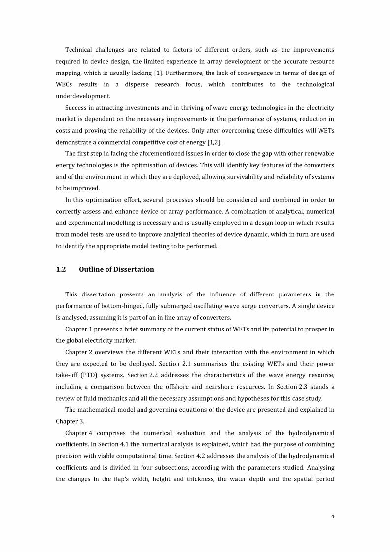
The classification of WECs can be done according to different characteristics as shown in Fig.

2-1, where a summary of different typical classifications for wave energy converters is given. These

classifications are not unique and other kinds of classification can be used, such as the classification

presented in [6], for example.

Fig. 2-1 - Different classifications of WECs [1] (adapted)

7

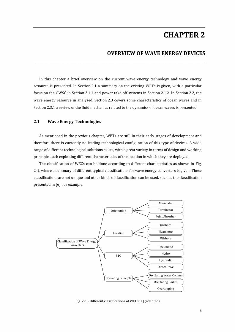
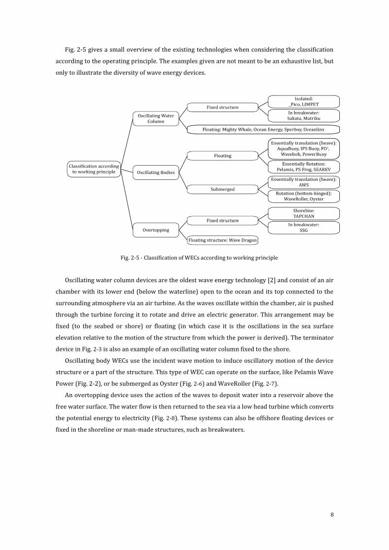
WECs are sometimes classified based on their orientation relative to the incoming waves as

attenuators, terminators or point absorbers. The targets of most of the research attention have

been point absorbers and attenuators [2,7]. Attenuators are devices which lie parallel to the

predominant direction of the incoming waves. An example of an attenuator device is Pelamis Wave

Power, developed by Ocean Power Delivery Ltd (Fig. 2-2). Terminators have their principal axis

parallel to the wave front, i.e. perpendicular to the predominant direction of the incoming waves

(Fig. 2-3), such as Pico Plant OWC deployed in the Azores. Point absorbers have small dimensions

relative to the incident wavelength in every direction and for this reason wave direction is not

important for these devices. An example of a point absorber WEC is Ocean Power Technology’s

Powerbuoy (Fig. 2-4).

According to Renzi and Dias [8], the OWSC that will be studied cannot be classified as either

attenuator, terminator or point absorber. Although it has its longer dimension parallel to the wave

crests, the dimensions of the device are too small relatively to the wavelength for this WEC to be

classified as terminator.

WECs can also be categorised referring to the distance to shore or water depth at which the

device or array is deployed using the terms “offshore”, “nearshore” or “onshore”, although there is

lack of consensus in what defines these locations.

Fig. 2-2 - Pelamis Wave Power [9] (adapted) Fig. 2-3 - Terminator [1] (adapted)

Fig. 2-4 - Point Absorber [1] (adapted)

8

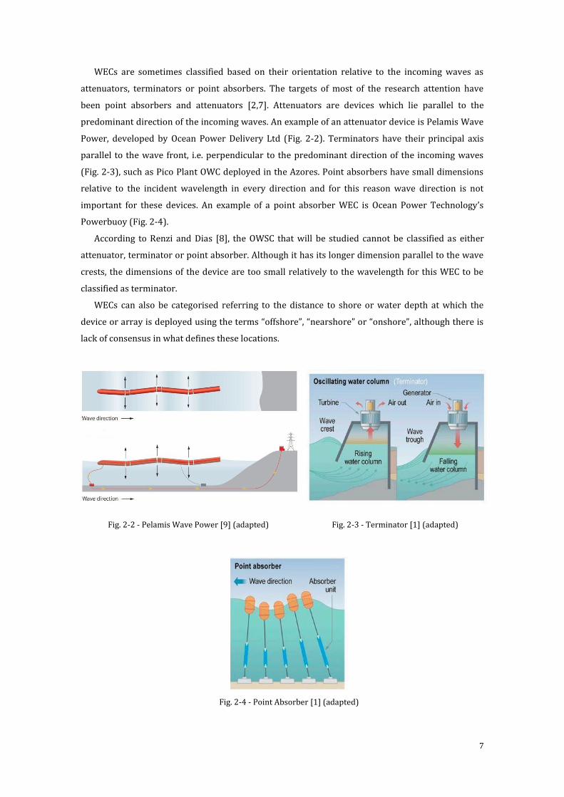
Fig. 2-5 gives a small overview of the existing technologies when considering the classification

according to the operating principle. The examples given are not meant to be an exhaustive list, but

only to illustrate the diversity of wave energy devices.

Fig. 2-5 - Classification of WECs according to working principle

Oscillating water column devices are the oldest wave energy technology [2] and consist of an air

chamber with its lower end (below the waterline) open to the ocean and its top connected to the

surrounding atmosphere via an air turbine. As the waves oscillate within the chamber, air is pushed

through the turbine forcing it to rotate and drive an electric generator. This arrangement may be

fixed (to the seabed or shore) or floating (in which case it is the oscillations in the sea surface

elevation relative to the motion of the structure from which the power is derived). The terminator

device in Fig. 2-3 is also an example of an oscillating water column fixed to the shore.

Oscillating body WECs use the incident wave motion to induce oscillatory motion of the device

structure or a part of the structure. This type of WEC can operate on the surface, like Pelamis Wave

Power (Fig. 2-2), or be submerged as Oyster (Fig. 2-6) and WaveRoller (Fig. 2-7).

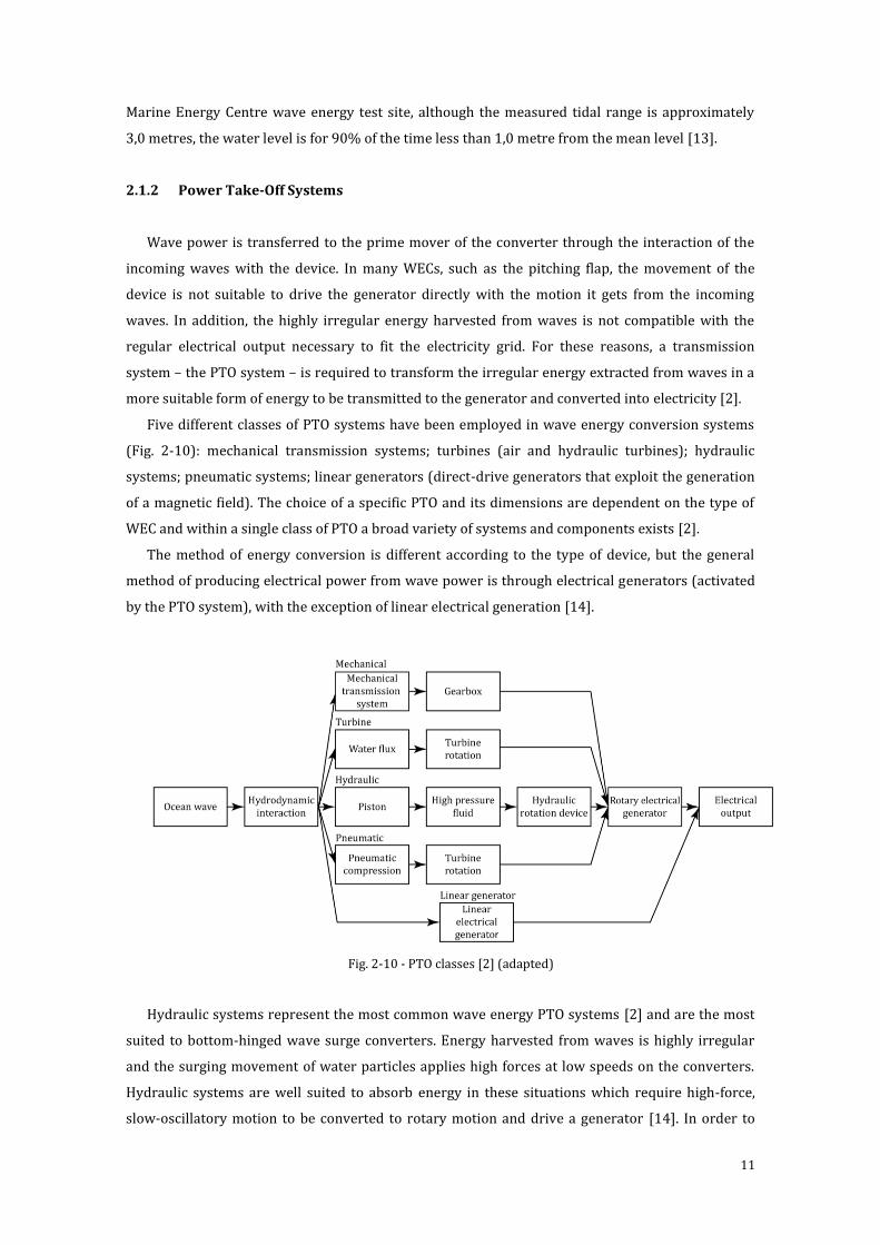
An overtopping device uses the action of the waves to deposit water into a reservoir above the

free water surface. The water flow is then returned to the sea via a low head turbine which converts

the potential energy to electricity (Fig. 2-8). These systems can also be offshore floating devices or

fixed in the shoreline or man-made structures, such as breakwaters.

9

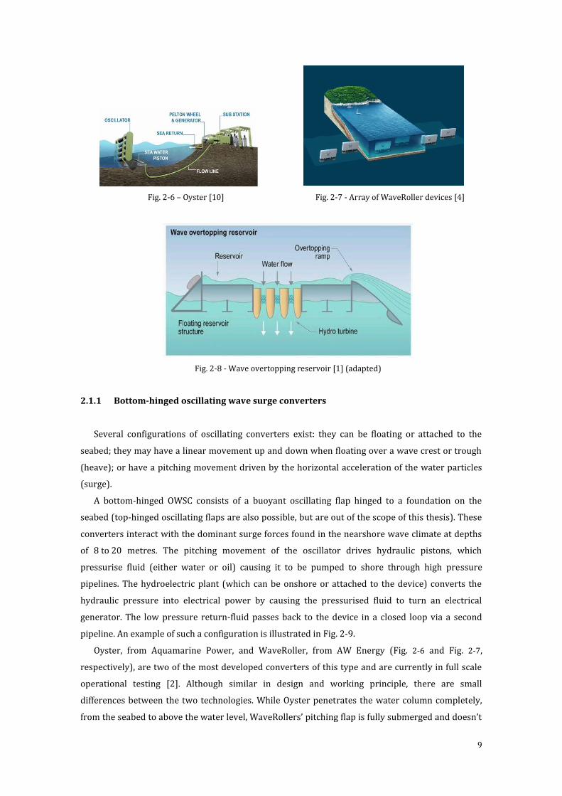
Fig. 2-6 – Oyster [10]

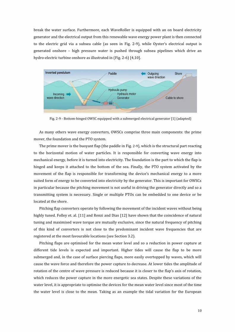
Fig. 2-7 - Array of WaveRoller devices [4]

Fig. 2-8 - Wave overtopping reservoir [1] (adapted)

2.1.1 Bottom-hinged oscillating wave surge converters

Several configurations of oscillating converters exist: they can be floating or attached to the

seabed; they may have a linear movement up and down when floating over a wave crest or trough

(heave); or have a pitching movement driven by the horizontal acceleration of the water particles

(surge).

A bottom-hinged OWSC consists of a buoyant oscillating flap hinged to a foundation on the

seabed (top-hinged oscillating flaps are also possible, but are out of the scope of this thesis). These

converters interact with the dominant surge forces found in the nearshore wave climate at depths

of 8 to 20 metres. The pitching movement of the oscillator drives hydraulic pistons, which

pressurise fluid (either water or oil) causing it to be pumped to shore through high pressure

pipelines. The hydroelectric plant (which can be onshore or attached to the device) converts the

hydraulic pressure into electrical power by causing the pressurised fluid to turn an electrical

generator. The low pressure return-fluid passes back to the device in a closed loop via a second

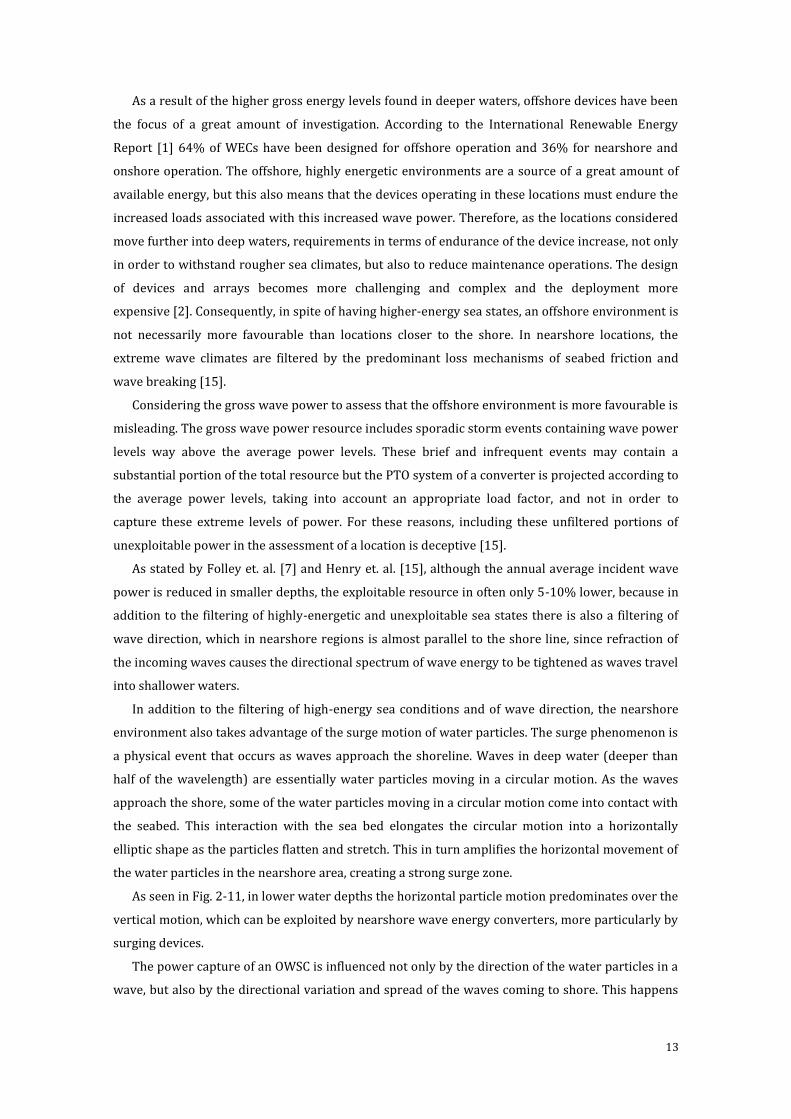
pipeline. An example of such a configuration is illustrated in Fig. 2-9.

Oyster, from Aquamarine Power, and WaveRoller, from AW Energy (Fig. 2-6 and Fig. 2-7,

respectively), are two of the most developed converters of this type and are currently in full scale

operational testing [2]. Although similar in design and working principle, there are small

differences between the two technologies. While Oyster penetrates the water column completely,

from the seabed to above the water level, WaveRollers’ pitching flap is fully submerged and doesn’t

10

break the water surface. Furthermore, each WaveRoller is equipped with an on board electricity

generator and the electrical output from this renewable wave energy power plant is then connected

to the electric grid via a subsea cable (as seen in Fig. 2-9), while Oyster’s electrical output is

generated onshore – high pressure water is pushed through subsea pipelines which drive an

hydro-electric turbine onshore as illustrated in (Fig. 2-6) [4,10].

Fig. 2-9 - Bottom-hinged OWSC equipped with a submerged electrical generator [1] (adapted)

As many others wave energy converters, OWSCs comprise three main components: the prime

mover, the foundation and the PTO system.

The prime mover is the buoyant flap (the paddle in Fig. 2-9), which is the structural part reacting

to the horizontal motion of water particles. It is responsible for converting wave energy into

mechanical energy, before it is turned into electricity. The foundation is the part to which the flap is

hinged and keeps it attached to the bottom of the sea. Finally, the PTO system activated by the

movement of the flap is responsible for transforming the device’s mechanical energy to a more

suited form of energy to be converted into electricity by the generator. This is important for OWSCs

in particular because the pitching movement is not useful in driving the generator directly and so a

transmitting system is necessary. Single or multiple PTOs can be embedded to one device or be

located at the shore.

Pitching flap converters operate by following the movement of the incident waves without being

highly tuned. Folley et. al. [11] and Renzi and Dias [12] have shown that the coincidence of natural

tuning and maximised wave torque are mutually exclusive, since the natural frequency of pitching

of this kind of converters is not close to the predominant incident wave frequencies that are

registered at the most favourable locations (see Section 3.2).

Pitching flaps are optimised for the mean water level and so a reduction in power capture at

different tide levels is expected and important. Higher tides will cause the flap to be more

submerged and, in the case of surface piercing flaps, more easily overtopped by waves, which will

cause the wave force and therefore the power capture to decrease. At lower tides the amplitude of

rotation of the centre of wave pressure is reduced because it is closer to the flap’s axis of rotation,

which reduces the power capture in the more energetic sea states. Despite these variations of the

water level, it is appropriate to optimise the devices for the mean water level since most of the time

the water level is close to the mean. Taking as an example the tidal variation for the European

11

Marine Energy Centre wave energy test site, although the measured tidal range is approximately

3,0 metres, the water level is for 90% of the time less than 1,0 metre from the mean level [13].

2.1.2 Power Take-Off Systems

Wave power is transferred to the prime mover of the converter through the interaction of the

incoming waves with the device. In many WECs, such as the pitching flap, the movement of the

device is not suitable to drive the generator directly with the motion it gets from the incoming

waves. In addition, the highly irregular energy harvested from waves is not compatible with the

regular electrical output necessary to fit the electricity grid. For these reasons, a transmission

system – the PTO system – is required to transform the irregular energy extracted from waves in a

more suitable form of energy to be transmitted to the generator and converted into electricity [2].

Five different classes of PTO systems have been employed in wave energy conversion systems

(Fig. 2-10): mechanical transmission systems; turbines (air and hydraulic turbines); hydraulic

systems; pneumatic systems; linear generators (direct-drive generators that exploit the generation

of a magnetic field). The choice of a specific PTO and its dimensions are dependent on the type of

WEC and within a single class of PTO a broad variety of systems and components exists [2].

The method of energy conversion is different according to the type of device, but the general

method of producing electrical power from wave power is through electrical generators (activated

by the PTO system), with the exception of linear electrical generation [14].

Fig. 2-10 - PTO classes [2] (adapted)

Hydraulic systems represent the most common wave energy PTO systems [2] and are the most

suited to bottom-hinged wave surge converters. Energy harvested from waves is highly irregular

and the surging movement of water particles applies high forces at low speeds on the converters.

Hydraulic systems are well suited to absorb energy in these situations which require high-force,

slow-oscillatory motion to be converted to rotary motion and drive a generator [14]. In order to

12

rectify the fluctuating wave power, which would result in variable electrical power output unsuited

to the electrical grid, some sort of energy storage system (or other means of compensation, such as

an array of devices) is usually incorporated in the PTO system, such as accumulators, which can

function as short term energy storage, helping the system handle the fluctuations [14]. Hydraulic

PTOs comprise several different parts connecting the hydraulic cylinder to the hydraulic motor

(Fig. 2-9) which allow power to be regulated, such as check valves, throttling valves, accumulators

and flywheels [13].

In addition to the different PTO systems, different control strategies have also been developed.

Since waves in real seas do not have constant height and frequency, a requirement of a WEC is to

adapt to these continuous changes and behave as resonant over the range of different frequencies.

The level of adaptation can range from adjusting the parameters of the device to a particular set of

sea state conditions to wave by wave adaptation (fast tuning). The different control strategies, such

as latching control, phase control and fast tuning, are out of the scope of this thesis. These concepts

are studied in detail in [14].

2.2 Wave Energy Resource

Wave energy is a result of the transfer of kinetic energy from the wind to the surface of the

ocean water and, since it is solar energy that creates the differences in air temperature that cause

wind, wave energy can be considered a concentrated form of solar energy.

Kinetic energy is transferred to the water when wind pushes against small ripples or waves on

the surface, causing the waves to grow and travel forward. In deep water, waves can propagate

through long distances without significant energy loss and will continue to accumulate energy from

the wind over long extents of open ocean until their energy dissipates on distant shores. The

interaction between the waves and the sea bottom gradually reduces the energy level in the waves

and the amount of energy transferred between wind and water is a function of different factors: the

wind speed, the extent of water over which the wind blows (fetch) and the amount of time the wind

blows [1,4].

Due to the Earth’s rotation and the westerly direction of predominant winds, high wave power

regions are usually located along the western coasts of the continents, particularly in locations

where waves can travel long distances without facing any obstacles [4].

Ocean waves have a low potential for sudden changes and sea states can be accurately predicted

more than 48 hours in advance, in contrast with accurate wind forecasts, which are only available

5-7 hours beforehand. Furthermore, due to the natural phenomena of refraction and reflection,

directions of waves near the shore can be determined in advance [14].

According to Drew et. al. [14], wave energy converters can generate power up to 90% of their

working time, compared to 20-30% for solar or wind energy devices. The wave energy resource is

consistent, with waves arriving 24 hours per day, and seasonality occurs at a large scale of time,

with higher wave conditions experienced in the winter than in the summer at most locations.

13

As a result of the higher gross energy levels found in deeper waters, offshore devices have been

the focus of a great amount of investigation. According to the International Renewable Energy

Report [1] 64% of WECs have been designed for offshore operation and 36% for nearshore and

onshore operation. The offshore, highly energetic environments are a source of a great amount of

available energy, but this also means that the devices operating in these locations must endure the

increased loads associated with this increased wave power. Therefore, as the locations considered

move further into deep waters, requirements in terms of endurance of the device increase, not only

in order to withstand rougher sea climates, but also to reduce maintenance operations. The design

of devices and arrays becomes more challenging and complex and the deployment more

expensive [2]. Consequently, in spite of having higher-energy sea states, an offshore environment is

not necessarily more favourable than locations closer to the shore. In nearshore locations, the

extreme wave climates are filtered by the predominant loss mechanisms of seabed friction and

wave breaking [15].

Considering the gross wave power to assess that the offshore environment is more favourable is

misleading. The gross wave power resource includes sporadic storm events containing wave power

levels way above the average power levels. These brief and infrequent events may contain a

substantial portion of the total resource but the PTO system of a converter is projected according to

the average power levels, taking into account an appropriate load factor, and not in order to

capture these extreme levels of power. For these reasons, including these unfiltered portions of

unexploitable power in the assessment of a location is deceptive [15].

As stated by Folley et. al. [7] and Henry et. al. [15], although the annual average incident wave

power is reduced in smaller depths, the exploitable resource in often only 5-10% lower, because in

addition to the filtering of highly-energetic and unexploitable sea states there is also a filtering of

wave direction, which in nearshore regions is almost parallel to the shore line, since refraction of

the incoming waves causes the directional spectrum of wave energy to be tightened as waves travel

into shallower waters.

In addition to the filtering of high-energy sea conditions and of wave direction, the nearshore

environment also takes advantage of the surge motion of water particles. The surge phenomenon is

a physical event that occurs as waves approach the shoreline. Waves in deep water (deeper than

half of the wavelength) are essentially water particles moving in a circular motion. As the waves

approach the shore, some of the water particles moving in a circular motion come into contact with

the seabed. This interaction with the sea bed elongates the circular motion into a horizontally

elliptic shape as the particles flatten and stretch. This in turn amplifies the horizontal movement of

the water particles in the nearshore area, creating a strong surge zone.

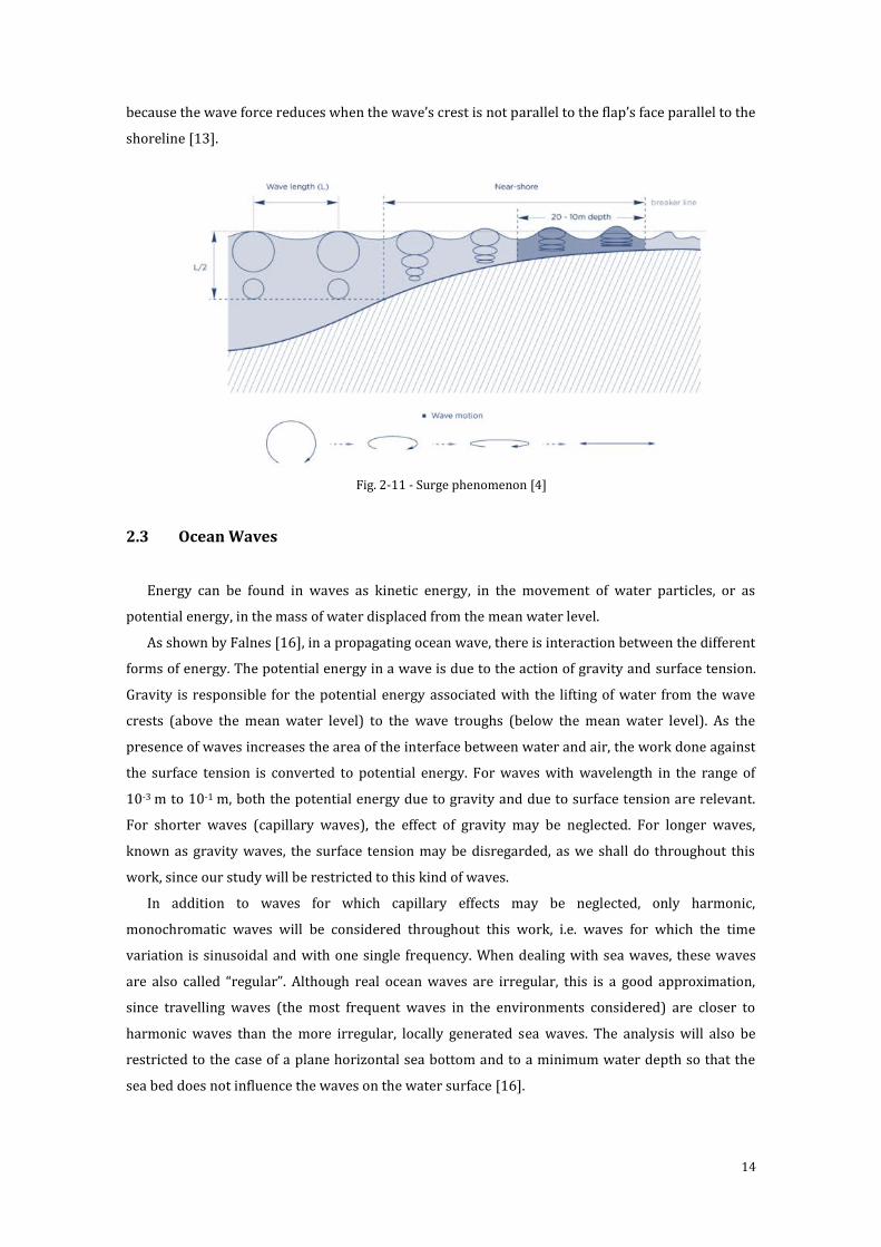
As seen in Fig. 2-11, in lower water depths the horizontal particle motion predominates over the

vertical motion, which can be exploited by nearshore wave energy converters, more particularly by

surging devices.

The power capture of an OWSC is influenced not only by the direction of the water particles in a

wave, but also by the directional variation and spread of the waves coming to shore. This happens

14

because the wave force reduces when the wave’s crest is not parallel to the flap’s face parallel to the

shoreline [13].

Fig. 2-11 - Surge phenomenon [4]

2.3 Ocean Waves

Energy can be found in waves as kinetic energy, in the movement of water particles, or as

potential energy, in the mass of water displaced from the mean water level.

As shown by Falnes [16], in a propagating ocean wave, there is interaction between the different

forms of energy. The potential energy in a wave is due to the action of gravity and surface tension.

Gravity is responsible for the potential energy associated with the lifting of water from the wave

crests (above the mean water level) to the wave troughs (below the mean water level). As the

presence of waves increases the area of the interface between water and air, the work done against

the surface tension is converted to potential energy. For waves with wavelength in the range of

10-3 m to 10-1 m, both the potential energy due to gravity and due to surface tension are relevant.

For shorter waves (capillary waves), the effect of gravity may be neglected. For longer waves,

known as gravity waves, the surface tension may be disregarded, as we shall do throughout this

work, since our study will be restricted to this kind of waves.

In addition to waves for which capillary effects may be neglected, only harmonic,

monochromatic waves will be considered throughout this work, i.e. waves for which the time

variation is sinusoidal and with one single frequency. When dealing with sea waves, these waves

are also called “regular”. Although real ocean waves are irregular, this is a good approximation,

since travelling waves (the most frequent waves in the environments considered) are closer to

harmonic waves than the more irregular, locally generated sea waves. The analysis will also be

restricted to the case of a plane horizontal sea bottom and to a minimum water depth so that the

sea bed does not influence the waves on the water surface [16].

15

2.3.1 Governing Equations and Water-Solid Interaction

In this section, gravity waves on an ideal, incompressible fluid will be studied. It is assumed that

wave motion takes place without loss of mechanical energy, that the fluid motion is irrotational and

also that the wave amplitude is so small that linear theory is applicable.

As demonstrated in the literature [16,17] the conservation of mass and momentum in a fluid are

expressed, respectively, by the continuity equation

𝜕𝜌

𝜕𝑡+ ∇ ∙ (𝜌�⃗�) = 0 (2.1)

and the Navier Stokes equation

𝐷�⃗⃗�

𝐷𝑡≡𝜕�⃗⃗�

𝜕𝑡+ (�⃗⃗� ∙ ∇)�⃗⃗� = −

1

𝜌∇𝑝 + 𝜈𝑘∇

2�⃗⃗� +1

𝜌�⃗⃗� (2.2)

In (2.1) and (2.2) ρ is the density of the fluid, which in this case is ocean water, t is time, �⃗� is

the velocity of the element of flowing fluid, p is the pressure of the fluid, 𝜈𝑘 is the kinematic

viscosity coefficient and 𝑓 is the external force per unit volume of fluid. Here we are considering

only the force due to gravity, that is,

𝑓 = 𝜌�⃗� (2.3)

where �⃗� is the acceleration due to gravity. Taking into account the assumptions made at the

beginning of this section, two important simplifications to the conservation equations can be made.

Considering ideal fluid, which is inviscid fluid, then 𝜈𝑘 = 0 and the term depending on the

kinematic viscosity coefficient disappears. Also, the assumption of incompressible fluid means that

the density ρ is constant in time and space and so the continuity and Navier-Stokes equations can

be rewritten in the following way:

∇ ∙ �⃗� = 0 (2.4)

𝜕�⃗�

𝜕𝑡+ �⃗� ∙ ∇�⃗� = −

1

𝜌∇𝑝 + �⃗� (2.5)

Considering the assumption of irrotational fluid, there is a velocity potential, Φ, such as

�⃗� = ∇Φ (2.6)

Combining (2.4) and (2.6) we get the Laplace equation

16

∇2Φ = 0 (2.7)

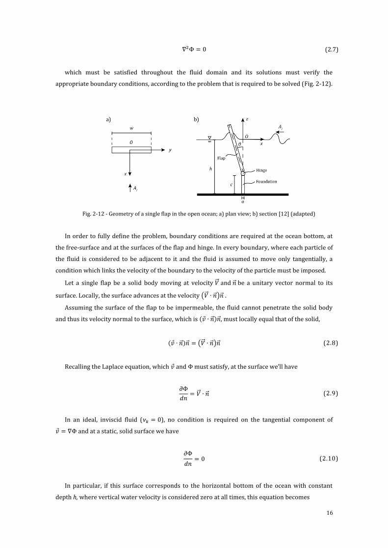
which must be satisfied throughout the fluid domain and its solutions must verify the

appropriate boundary conditions, according to the problem that is required to be solved (Fig. 2-12).

Fig. 2-12 - Geometry of a single flap in the open ocean; a) plan view; b) section [12] (adapted)

In order to fully define the problem, boundary conditions are required at the ocean bottom, at

the free-surface and at the surfaces of the flap and hinge. In every boundary, where each particle of

the fluid is considered to be adjacent to it and the fluid is assumed to move only tangentially, a

condition which links the velocity of the boundary to the velocity of the particle must be imposed.

Let a single flap be a solid body moving at velocity �⃗⃗� and �⃗⃗� be a unitary vector normal to its

surface. Locally, the surface advances at the velocity (�⃗⃗� ∙ �⃗⃗�)�⃗⃗� .

Assuming the surface of the flap to be impermeable, the fluid cannot penetrate the solid body

and thus its velocity normal to the surface, which is (�⃗� ∙ �⃗⃗�)�⃗⃗�, must locally equal that of the solid,

(�⃗� ∙ �⃗⃗�)�⃗⃗� = (�⃗⃗� ∙ �⃗⃗�)�⃗⃗� (2.8)

Recalling the Laplace equation, which �⃗� and Φ must satisfy, at the surface we’ll have

𝜕Φ

𝑑𝑛= �⃗⃗� ∙ �⃗⃗� (2.9)

In an ideal, inviscid fluid (𝜈𝑘 = 0), no condition is required on the tangential component of

�⃗� = ∇Φ and at a static, solid surface we have

𝜕Φ

𝑑𝑛= 0 (2.10)

In particular, if this surface corresponds to the horizontal bottom of the ocean with constant

depth h, where vertical water velocity is considered zero at all times, this equation becomes

17

𝜕Φ

𝑑𝑧= 0 𝑎𝑡 𝑧 = −ℎ (2.11)

Equation (2.11) is the first defined boundary condition for this problem.

On the free surface 𝑧 = 𝜂(𝑥, 𝑦, 𝑡), which is the interface between water and open air, two

boundary conditions are necessary: one to assure that the fluid particles on the surface stay on the

surface (kinematic boundary condition) and another one to relate the fluid pressure to the

atmospheric pressure (dynamic boundary condition).

As stated in [17], the fluid particles near the surface remain near the surface as long as the

waves don’t break, i.e. as long as the wave motion is smooth. Let us consider one particle of fluid

moving along the surface η, from point (𝑥1, 𝜂1) to point (𝑥2, 𝜂2) with velocity �⃗� during the time

interval of ∆𝑡 = 𝑡2 − 𝑡1. The coordinates of the final position of the particle can be written as

𝑥2 = 𝑥1 + 𝑣𝑥(𝑡2 − 𝑡1) (2.12 a)

𝜂2= 𝜂

1+ 𝑣𝑧(𝑡2 − 𝑡1) (2.12 b)

Following [16,17], expanding 𝜂2(𝑥2, 𝑡2) in a Taylor series

𝜂(𝑥2, 𝑡2) = 𝜂(𝑥1, 𝑡2) +

𝜕𝜂

𝜕𝑥(𝑥1, 𝑡2). (𝑥2 − 𝑥1) … (2.13)

Introducing the expansion in (2.12 a) and divided by (𝑡2 − 𝑡1) letting 𝑡2 → 𝑡1

𝜕𝜂

𝜕𝑡+ 𝑣𝑥

𝜕𝜂

𝜕𝑥= 𝑣𝑧 (2.14)

This equation is the boundary condition at the free surface and states in mathematical terms

that a fluid particle at the surface should remain at the surface at all times. This boundary condition

regards the motion of the water surface and for this reason it is usually called the kinematic

boundary condition.

The dynamic boundary condition assures that the pressure p at the water surface is equal to the

atmospheric pressure, which is assumed to be constant. Applying Bernoulli’s Equation to the

surface line where 𝑧 = 𝜂(𝑥, 𝑦, 𝑡)

𝜕Φ

𝜕𝑡+1

2(∇Φ ∙ ∇Φ) + 𝑔𝜂 = 0 (2.15)

This condition deals with the forces on the surface and is therefore defined as the dynamic

boundary condition.

18

Boundary conditions (2.14) and (2.15) can be linearised if we assume that the dynamic

variables such as Φ, η and all their derivatives are small and we neglect small terms of second or

higher order, such as 𝑣2 = ∇𝜑 ∙ ∇𝜑. Then, equations (2.14) and (2.15) can respectively be

rewritten as

𝜕Φ

𝜕𝑡= 𝑣𝑧 =

𝜕𝜂

𝜕𝑡 (2.16)

𝜕Φ

𝜕𝑡+ 𝑔𝜂 = 0 (2.17)

Taking the time derivative of the dynamic boundary condition (2.16) and inserting into the

kinetic boundary condition (2.17), we get the linearised dynamic-kinematic condition (2.18).

[𝜕2Φ

𝜕𝑡2+ 𝑔

𝜕Φ

𝜕𝑧]𝑧=0

= 0 (2.18)

The boundary condition expressed by (2.10) has to be satisfied on the wet surface of the

moving body as well. However, if the body is performing small-amplitude oscillations, we may

make the linearising approximation that the boundary condition (2.10) is to be applied at the

time-average (or equilibrium) position of the wet surface of an oscillating body.

Conditions (2.7), (2.11) and (2.16)-(2.18) are appropriate to any open ocean problem using

the approximations explained. As shown in [13] and [18], further boundary conditions are

necessary to the specific problem in study and will be discussed in Section 3.1.

19

3CHAPTER 3

NUMERICAL INVESTIGATION OF A SURGING WEC ______________________________________________________________

The dynamics of OWSCs can be modelled and analysed in many different ways, each being more

or less suitable for specific purposes according to its characteristics. For instance, inviscid

irrotational analytical models can identify the maximum power capture of a particular system

accurately, though they may be less useful in determining what the actual performance will be due

to the effect of motion constraints and viscous losses. On the other hand, modelling recurring to

wave tanks is useful in providing performance data for determining the expected productivity of a

particular prototype, but it is less helpful in identifying how the prototype design may be improved.

To clearly understand the dynamics of a device the model must be executed in such a way that

key elements that have an influence on performance can be clearly identified and the effects of

changing these elements can be easily evaluated. In these models, it is more important to correctly

model comparative performances than to make a predictive model of exact values.

In this chapter the mathematical model and governing equations of the system are introduced

by taking as reference the works of Renzi and Dias [12,18]. The necessary assumptions and

hypothesis are explained and the governing equations are presented.

3.1 Analytical Model

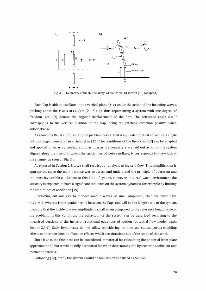
Let us consider an in-line array of bottom-hinged converters as illustrated in Fig. 3-1 a), parallel

to the shoreline, in an open ocean of constant depth h. Each converter of the array – Fig. 3-1 b) – is

treated as a rectangular flap of width w, height hf and thickness a and is placed upon a foundation of

height c. The flaps oscillate about a hinge (which is assumed to be frictionless) under the action of

monochromatic, regular incident waves of period T and amplitude AI, coming from the right side as

represented in Fig. 3-1. Since the practical application of such a system is typically in the nearshore,

where wave fronts are almost parallel to the shoreline because of refraction [15], all the incoming

wave fronts are assumed to be parallel to the width of the flap (obliquely incident waves are out of

the scope of this work).

A Cartesian system of reference O (x, y, z) is set at an origin O on the water level, aligned with the

centre of the flap when it is in a vertical position. The x axis is parallel to the water surface and its

direction is parallel and opposite to the direction of the incoming waves. The y axis is parallel to the

width of the devices and aligned with their centre. Finally the z axis points upwards from the water

level.

20

Fig. 3-1 - Geometry of the in-line array; a) plan view; b) section [18] (adapted)

Each flap is able to oscillate on the vertical plane (𝑥, 𝑧) under the action of the incoming waves,

pitching about the y axis at (𝑥, 𝑧) = (0, −ℎ + 𝑐), thus representing a system with one degree of

freedom. Let θ(t) denote the angular displacement of the flap. The reference angle θ = 0°

corresponds to the vertical position of the flap, being the pitching direction positive when

anticlockwise.

As shown by Renzi and Dias [18] the problem here stated is equivalent to that solved for a single

bottom-hinged converter in a channel in [12]. The conditions of the theory in [12] can be adapted

and applied to an array configuration, as long as the converters are laid out as an in-line system

aligned along the y axis, in which the spatial period between flaps, b, corresponds to the width of

the channel, as seen on Fig. 3-1.

As exposed in Section 2.3.1, we shall restrict our analysis to inviscid flow. This simplification is

appropriate since the main purpose was to assess and understand the principle of operation and

the most favourable conditions to this kind of system. However, in a real-wave environment the

viscosity is expected to have a significant influence on the system dynamics, for example by limiting

the amplitudes of oscillation [19].

Restricting our analysis to monochromatic waves of small amplitude, then we must have

𝐴𝐼/𝑏 ≪ 1, where b is the spatial period between the flaps and will be the length scale of the system,

meaning that the incident wave amplitude is small when compared to the reference length scale of

the problem. In this condition, the behaviour of the system can be described recurring to the

linearised versions of the inviscid-irrotational equations of motion (potential flow model, again

Section 2.3.1). Such hypotheses do not allow considering random-sea states, vortex-shedding

effects neither non-linear diffraction effects, which are situations out of the scope of this work.

Since 𝑏 ≫ 𝑎, the thickness can be considered immaterial for calculating the potential (thin-plate

approximation), but it will be fully accounted for when determining the hydrostatic coefficient and

moment of inertia.

Following [12], firstly the system should be non-dimensionalised as follows:

21

(𝑥′, 𝑦′, 𝑧′, 𝑤′, ℎ′𝑓, 𝑎′, ℎ′, 𝑐′) =

(𝑥, 𝑦, 𝑧, 𝑤, ℎ𝑓, 𝑎, ℎ, 𝑐)

𝑏 (3.1)

𝑡′ = √

𝑔

𝑏 𝑡 (3.2)

𝜃′ =

𝑏

𝐴𝜃 (3.3)

Φ′ =

1

√𝑔𝑏𝐴Φ (3.4)

Primes distinguish non-dimensional from dimensional physical quantities and A is the

amplitude scale of the wave field.

The linear governing equations that must be verified by the linearised velocity potential Φ’, are

derived assuming small-amplitude oscillations of the flap. Then, the pitching angle of the device can

also be considered small and the behaviour of the system may be treated as linear and so may the

boundary conditions associated to the geometry in study [12,20], which are those explained in

Section 2.3.1 and two others related to the specific geometry of this problem.

Recalling the Laplace Equation (2.7) and the boundary conditions explained in Section

2.3.1 - no-flux condition on the bottom of the ocean (2.11) and linearised kinematic-dynamic

boundary condition (2.18) – these can now be rewritten in their non-dimensional form:

∇′2Φ′(𝑥′, 𝑦′, 𝑧′, 𝑡′) = 0 (3.5)

𝜕Φ′

𝜕𝑧′= 0, for 𝑧′ = −ℎ′ (3.6)

∂2Φ′

∂t′2 + g

∂Φ′

∂z′= 0, for z′ = 0 (3.7)

Two additional boundary conditions should be considered attending to the specific geometry of

the device, assuring only tangential motion along the lateral surfaces of the flap, i.e. assuring

impermeability of the device. As shown in [12,18], applying the thin-body approximation to the

flap, expression (2.9) for the pitching motion about the y’ axis yields

𝜕Φ′

𝜕𝑥′= −

𝜕𝜃′(𝑡′)

𝜕𝑡′(𝑧′ + ℎ′ − 𝑐′) 𝐻(𝑧′ + ℎ′ − 𝑐′), x′ = ±0, |y′| < w′/2 (3.8)

along the flap sides normal to the x’ axis, where the Heaviside step function H is used to model

the absence of flow through the bottom foundation, and

𝜕Φ′

𝜕𝑦′= 0 (3.9)

along the flap sides normal to the y’ axis.

22

3.2 Body Motion

Referring again to Fig. 3-1, the movement of each flap resembles that of an inverted pendulum.

Subjected to the simple, harmonic perturbation of the incoming waves, the flap oscillates about its

equilibrium position (θ = 0°). In order to study the movement of the oscillating flap, we should first

consider all the moments applied on the system, applying Newton’s second law of motion

𝐼�̈� = 𝒯 (3.10)

where I is the moment of inertia about the y axis, �̈� is the angular acceleration and 𝒯 is the sum

of all the moments applied on the flap. The right-hand term of the above equation should comprise

both the action of the water and the action of the PTO system over the flap. Considering these

actions exerted over the plate as partly inertial, partly elastic and partly damped, the behaviour of

the flap can be modelled as a forced damped oscillator. Denoting M, D and E as the inertial, damping

and elastic coefficients of the system, respectively, and ℱ as the sum of the external torque applied

on the plate, the motion equation of the device shall have the form

𝑀�̈�(𝑡) = 𝐷�̇�(𝑡) + 𝐸𝜃(𝑡) + ℱ (3.11)

In (3.11), M, D and E should be replaced with their corresponding contributions. The inertial

term comprehends the moment of inertia of the flap, I, and the added inertia due to the mass of the

water displaced by the flap with its movement, μ. Also, the inertial characteristic of the PTO system,

μpto, should be included in this term. In the damping coefficient, D, are included the damping

characteristic of the PTO system (or rate of power take-off), 𝜈𝑝𝑡𝑜, and the damping due to the

radiation of the incoming waves, 𝜈. Finally, the elastic term considers the elastic characteristic of

the PTO system, Cpto, and also the elastic characteristic of the flap given by the hydrostatic restoring

coefficient, C, which is a restoring moment due to the buoyancy of the flap (the effect of the

buoyancy of the flap as it attempts to go back to the vertical position). Replacing these terms in

(3.11) and rewriting it non-dimensionally in the frequency domain, the motion equation of the

pitching flap becomes:

[−𝜔′2(𝐼′ + 𝜇′ + 𝜇′

𝑝𝑡𝑜) + 𝐶′ + 𝐶′𝑝𝑡𝑜 − 𝑖𝜔′(𝜈′ + 𝜈′𝑝𝑡𝑜)] Θ′ = 𝐹′ (3.12)

As before, primes denote non-dimensional physical quantities, ω’ is the non-dimensional

frequency of the incoming waves and Θ is the unknown complex amplitude of rotation of the flap

and in order to determine its value using equation (3.12) and fully define the flap motion all the

other variables must be known.

Consider the geometry of each flap as a rectangular prism, as mentioned before, with width w,

height hf and thickness a. In a first approach, with the purpose of explaining how the movement of

23

the flap can be determined using expression (3.12), the PTO system will be considered as a

damper, i.e. 𝜇𝑝𝑡𝑜 = 𝐶𝑝𝑡𝑜 = 0. Consequently, the inertial, elastic and damping coefficients of equation

(3.12) will depend only on the geometry of the flap and are easily calculated using the values

chosen for the geometric properties.

The moment of inertia about the pitching axis is [19]

𝐼 =

𝜌𝑓𝑙𝑎𝑝 𝑡 𝑤 (h𝑓)3

3 (3.13)

and for it to be used in equation (3.12), it should also be written non-dimensionally, as follows:

𝐼′ =

𝐼

𝜌𝑓𝑙𝑎𝑝𝑏5

(3.14)

The hydrostatic restoring coefficient uses the assumption that the centre of gravity of the plate

coincides with the centre of buoyancy and that they are located at half of the height of the plate

[19]. Similarly to the moment of inertia, the dimensional and non-dimensional hydrostatic restoring

coefficients are, respectively:

𝐶 =

1 − 𝜌𝑓𝑙𝑎𝑝 𝜌𝑤⁄

2𝜌𝑤 𝑔 𝑡 𝑤 ℎ𝑓

2 (3.15)

𝐶′ =

𝐶

𝜌𝑓𝑙𝑎𝑝𝑔𝑏4 (3.16)

The added torque due to inertia, the radiation damping and the complex exciting torque

(corresponding to the action over the plate as if it was held fixed in incoming waves) depend on the

solutions of the waves’ radiation and scattering problems of this system. These problems were

addressed in the literature [12,20], in which it is demonstrated that

𝜇′ =

𝜋 𝑤′

4𝑅𝑒 {∑𝛼0𝑛𝑓𝑛

+∞

𝑛=0

} (3.17)

𝜈′ =

𝜔′ 𝜋 𝑤′

4𝐼𝑚 {∑𝛼0𝑛𝑓𝑛

+∞

𝑛=0

} (3.18)

𝐹′ = −

𝜋 𝑤′

4𝑖𝜔′𝐴′𝐼𝛽00𝑓0 (3.19)

In equations (3.17)-(3.19), fn are real constants and α0n and β00 are complex constants, all

dependent on the solutions of the dispersion relationship (3.20), where k’n are the non-dimensional

wavenumbers of the incoming waves with non-dimensional frequency ω’

24

𝜔′2 = 𝑘′ tanh(𝑘′ℎ′)

𝜔′2 = −𝑘′𝑛 tanh(𝑘′𝑛ℎ

′) 𝑛 = 1, 2, … , 𝑁 (3.20)

In this equation, 𝜅𝑛2 = 𝑘2 for 𝑛 = 0 and 𝜅𝑛

2 = −𝑘𝑛2 for 𝑛 ≫ 1. Then, fn is calculated using (3.21)

and α0n and β00 are determined solving the system in equation (3.22).

𝑓𝑛 =

√2 [𝜅′𝑛(ℎ′ − 𝑐′) sinh 𝜅𝑛ℎ + cosh 𝜅′𝑛𝑐′ − cosh 𝜅′𝑛ℎ′]

𝜅𝑛2(ℎ + 𝜔′−2 sinh2 𝜅′𝑛ℎ′)

1/2 (3.21)

∑{

𝛼𝑝𝑛𝛽𝑝𝑛

} 𝐶𝑝𝑛(𝑣0)

𝑃

𝑝=0

= −𝜋𝑤 {𝑓𝑛𝑑𝑛}, 𝑣0 ∈ (−1,1) (3.22)

In (3.22), 𝑝 = 0, 1, 2, … , 𝑃 and

𝑑0 =

𝑘 (ℎ + 𝜔−2 sinh2 𝑘ℎ)1/2

√2 𝜔 cosh 𝑘ℎ, 𝑑𝑛 = 0, 𝑛 = 1, 2, …, (3.23)

Cpn in equation (3.22) is a square matrix given by (3.24)

𝐶𝑝𝑛(𝑣0𝑗) = −𝜋 ∙ (𝑝 + 1) ∙ 𝑈𝑝(𝑣0𝑗) +𝑖𝜋𝜅𝑛𝑤

4

∙ ∫ (1 − 𝑢2)12 ∙ 𝑈𝑝(𝑢)

1

−1

∙ [𝑅𝑛 (

12𝜅𝑛𝑤|𝑣0 − 𝑢|)

|𝑣0 − 𝑢|+ ∑

𝐻1(1) (

12𝜅𝑛𝑤 |𝑣0 −

2𝑚𝑤− 𝑢|)

|𝑣0 −2𝑚𝑤− 𝑢|

+∞

𝑚=−∞,𝑚≠0

] 𝑑𝑢

(3.24)

In the above equations, P, N, m and the integration interval in (3.24) should be truncated by

numerical evaluation as will be explained in Section 4.1.

In (3.22) and (3.24), 𝑣0 ∈ (−1,1). The upper equation in (3.22) is for the coefficients 𝛼𝑝𝑛 of the

jump in the plane radiation potential across the plate, while the lower equation is for the

coefficients 𝛽𝑝𝑛 of the jump in the plane diffraction potential. Theoretically there exists an infinity

of points 𝑣0 ∈ (−1,1) where (3.22) can be evaluated, thus yielding a system of an infinite number of

equations (one for each 𝑣0) for an infinite number of unknowns. For (3.22) to be solved

numerically, the unknowns must be truncated to a finite integer number 𝑃 < ∞ and a finite number

of evaluation points 𝑣0 = 𝑣0𝑗 , 𝑗 = 0,1, … , 𝑃 must also be chosen in the domain (-1,1). (Parsons and

Martin, 1992) as cited by [12] showed that the fastest numerical convergence for such a system is

achieved when when 𝑣0𝑗 are the zeros of the Chebyshev polynomial of the first kind, i.e.

𝑣0𝑗 = cos

(2𝑗 + 1)𝜋

2𝑃 + 2, 𝑗 = 0,1, … , 𝑃 (3.25)

25

Hence (3.22) reduces to two (𝑃 + 1) × (𝑃 + 1) truncated algebraic systems for each n = 0, 1, 2....

For every value of n, there is a Cpn matrix in which the lines correspond to different values of p

and the rows to different values of 𝑣0𝑗 . This way, the following systems of equations are obtained

(again, for each value of n):

𝑛 = 0 →

{

𝛼00𝐶00(𝑣00) + 𝛼10𝐶10(𝑣00) + ⋯+ 𝛼𝑝0𝐶𝑝0(𝑣00) = −𝜋𝑤𝑓0𝛼00𝐶00(𝑣01) + 𝛼10𝐶10(𝑣01) + ⋯+ 𝛼𝑝0𝐶𝑝0(𝑣01) = −𝜋𝑤𝑓0

⋮𝛼00𝐶00(𝑣0𝑗) + 𝛼10𝐶10(𝑣0𝑗) + ⋯+ 𝛼𝑝0𝐶𝑝0(𝑣0𝑗) = −𝜋𝑤𝑓0

(3.27)

𝑛 = 1 →

{

𝛼01𝐶01(𝑣00) + 𝛼11𝐶11(𝑣00) + ⋯+ 𝛼𝑝1𝐶𝑝1(𝑣00) = −𝜋𝑤𝑓1𝛼01𝐶01(𝑣01) + 𝛼11𝐶11(𝑣01) + ⋯+ 𝛼𝑝1𝐶𝑝1(𝑣01) = −𝜋𝑤𝑓1

⋮𝛼01𝐶01(𝑣0𝑗) + 𝛼11𝐶11(𝑣0𝑗) + ⋯+ 𝛼𝑝1𝐶𝑝1(𝑣0𝑗) = −𝜋𝑤𝑓1

(3.28)

Solving all the N+1 systems of equations, 𝛼𝑝𝑛 and 𝛽𝑝𝑛 are determined. In order to solve these

systems, Cpn should be determined with equation (3.24), where the term

∫ (1 − 𝑢2)12 ∙ 𝑈𝑝(𝑢) ∙ [

𝑅𝑛 (12𝜅𝑛𝑤|𝑣0 − 𝑢|)

|𝑣0 − 𝑢|+ ∑

𝐻1(1) (

12𝜅𝑛𝑤 |𝑣0 −

2𝑚𝑤− 𝑢|)

|𝑣0 −2𝑚𝑤− 𝑢|

+∞

𝑚=−∞,𝑚≠0

] 𝑑𝑢1

−1

(3.29)

is solved numerically applying the Simpson’s rule, as in (3.30) where the length of the interval

𝐿 = 𝑏 − 𝑎 is determined as explained in Section 4.1.

∫ 𝑓(𝑢) 𝑑𝑢𝑏

𝑎

≈𝑏 − 𝑎

6 [𝑓(𝑎) + 4 ∙ 𝑓 (

𝑎 + 𝑏

2) + 𝑓(𝑏)] (3.30)

In (3.29) 𝑈𝑝(𝑢) are the Chebyshev polynomials of the second kind and order p, p = 0, 1, …, P, 𝐻1(1)

is the Hankel function of the first kind and first order calculated with the MATLAB function besselh

and

𝑅𝑛 (

1

2𝜅𝑛𝑤|𝑣0 − 𝑢|) = 𝐻1

(1)(1

2𝜅𝑛𝑤|𝑣0 − 𝑢|) −

4

𝑖𝜋

1

𝜅𝑛𝑤|𝑣0 − 𝑢| (3.31)

∑{𝛼𝑝𝑛}

𝑃

𝑝=0

. 𝐶𝑝𝑛(𝑣𝑜𝑗) = −𝜋 𝑤 𝑓𝑛

∑{𝛽𝑝𝑛}

𝑃

𝑝=0

. 𝐶𝑝𝑛(𝑣𝑜𝑗) = −𝜋 𝑤 𝑑𝑛

, 𝑗 = 0, 1, … , 𝑃 (3.26)

26

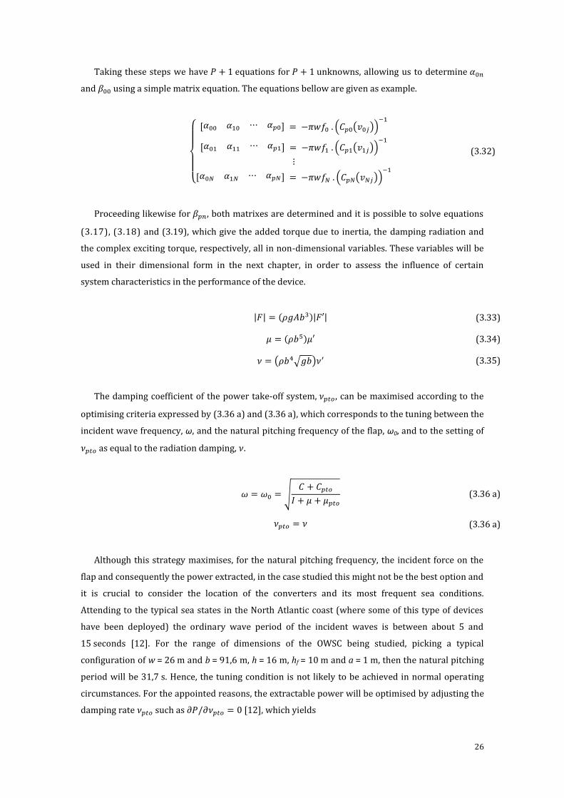
Taking these steps we have 𝑃 + 1 equations for 𝑃 + 1 unknowns, allowing us to determine 𝛼0𝑛

and 𝛽00 using a simple matrix equation. The equations bellow are given as example.

{

[𝛼00 𝛼10 ⋯ 𝛼𝑝0] = −𝜋𝑤𝑓0 . (𝐶𝑝0(𝑣0𝑗))

−1

[𝛼01 𝛼11 ⋯ 𝛼𝑝1] = −𝜋𝑤𝑓1 . (𝐶𝑝1(𝑣1𝑗))−1

⋮

[𝛼0𝑁 𝛼1𝑁 ⋯ 𝛼𝑝𝑁] = −𝜋𝑤𝑓𝑁 . (𝐶𝑝𝑁(𝑣𝑁𝑗))−1

(3.32)

Proceeding likewise for 𝛽𝑝𝑛, both matrixes are determined and it is possible to solve equations

(3.17), (3.18) and (3.19), which give the added torque due to inertia, the damping radiation and

the complex exciting torque, respectively, all in non-dimensional variables. These variables will be

used in their dimensional form in the next chapter, in order to assess the influence of certain

system characteristics in the performance of the device.

|𝐹| = (𝜌𝑔𝐴𝑏3)|𝐹′| (3.33)

𝜇 = (𝜌𝑏5)𝜇′ (3.34)

𝜈 = (𝜌𝑏4√𝑔𝑏)𝜈′ (3.35)

The damping coefficient of the power take-off system, 𝜈𝑝𝑡𝑜, can be maximised according to the

optimising criteria expressed by (3.36 a) and (3.36 a), which corresponds to the tuning between the

incident wave frequency, ω, and the natural pitching frequency of the flap, ω0, and to the setting of

𝜈𝑝𝑡𝑜 as equal to the radiation damping, 𝜈.

𝜔 = 𝜔0 = √

𝐶 + 𝐶𝑝𝑡𝑜

𝐼 + 𝜇 + 𝜇𝑝𝑡𝑜 (3.36 a)

𝜈𝑝𝑡𝑜 = 𝜈 (3.36 a)

Although this strategy maximises, for the natural pitching frequency, the incident force on the

flap and consequently the power extracted, in the case studied this might not be the best option and

it is crucial to consider the location of the converters and its most frequent sea conditions.

Attending to the typical sea states in the North Atlantic coast (where some of this type of devices

have been deployed) the ordinary wave period of the incident waves is between about 5 and

15 seconds [12]. For the range of dimensions of the OWSC being studied, picking a typical

configuration of w = 26 m and b = 91,6 m, h = 16 m, hf = 10 m and a = 1 m, then the natural pitching

period will be 31,7 s. Hence, the tuning condition is not likely to be achieved in normal operating

circumstances. For the appointed reasons, the extractable power will be optimised by adjusting the

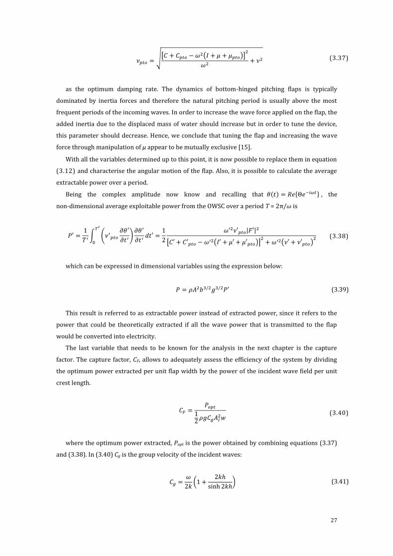
damping rate 𝜈𝑝𝑡𝑜 such as 𝜕𝑃/𝜕𝜈𝑝𝑡𝑜 = 0 [12], which yields

27

𝜈𝑝𝑡𝑜 =√[𝐶 + 𝐶𝑝𝑡𝑜 −𝜔

2(𝐼 + 𝜇 + 𝜇𝑝𝑡𝑜)]2

𝜔2+ 𝜈2 (3.37)

as the optimum damping rate. The dynamics of bottom-hinged pitching flaps is typically

dominated by inertia forces and therefore the natural pitching period is usually above the most

frequent periods of the incoming waves. In order to increase the wave force applied on the flap, the

added inertia due to the displaced mass of water should increase but in order to tune the device,

this parameter should decrease. Hence, we conclude that tuning the flap and increasing the wave

force through manipulation of μ appear to be mutually exclusive [15].

With all the variables determined up to this point, it is now possible to replace them in equation

(3.12) and characterise the angular motion of the flap. Also, it is possible to calculate the average

extractable power over a period.

Being the complex amplitude now know and recalling that 𝜃(𝑡) = 𝑅𝑒{Θ𝑒−𝑖𝜔𝑡} , the

non-dimensional average exploitable power from the OWSC over a period T = 2π/ω is

𝑃′ =

1

𝑇′∫ (𝜈′𝑝𝑡𝑜

𝜕𝜃′

𝜕𝑡′)𝜕𝜃′

𝜕𝑡′

𝑇′

0

𝑑𝑡′ =1

2

𝜔′2𝜈′𝑝𝑡𝑜|𝐹′|2

[𝐶′ + 𝐶′𝑝𝑡𝑜 − 𝜔′2(𝐼′ + 𝜇′ + 𝜇′𝑝𝑡𝑜)]

2+ 𝜔′2(𝜈′ + 𝜈′𝑝𝑡𝑜)

2 (3.38)

which can be expressed in dimensional variables using the expression below:

𝑃 = 𝜌𝐴2𝑏3/2𝑔3/2𝑃′ (3.39)

This result is referred to as extractable power instead of extracted power, since it refers to the

power that could be theoretically extracted if all the wave power that is transmitted to the flap

would be converted into electricity.

The last variable that needs to be known for the analysis in the next chapter is the capture

factor. The capture factor, CF, allows to adequately assess the efficiency of the system by dividing

the optimum power extracted per unit flap width by the power of the incident wave field per unit

crest length.

𝐶𝐹 =

𝑃𝑜𝑝𝑡12𝜌𝑔𝐶𝑔𝐴𝐼

2𝑤 (3.40)

where the optimum power extracted, Popt is the power obtained by combining equations (3.37)

and (3.38). In (3.40) Cg is the group velocity of the incident waves:

𝐶𝑔 =

𝜔

2𝑘(1 +

2𝑘ℎ

sinh 2𝑘ℎ) (3.41)

28

4CHAPTER 4

HYDRODYNAMICAL PERFORMANCE OF A SURGING WEC ______________________________________________________________

Following the formulation presented in the previous chapter, a MATLAB algorithm was

implemented in order to assess the hydrodynamical performance of the wave energy converter in

study. Once this algorithm was running properly, a numerical evaluation was necessary so that the

precision of the results could be improved without compromising the computation time needed to

execute the proposed calculations. After this numerical evaluation, which is explained in

Section 4.1, the hydrodynamical analysis was performed and the influence of the geometric

characteristics of the flap in the device performance was assessed.

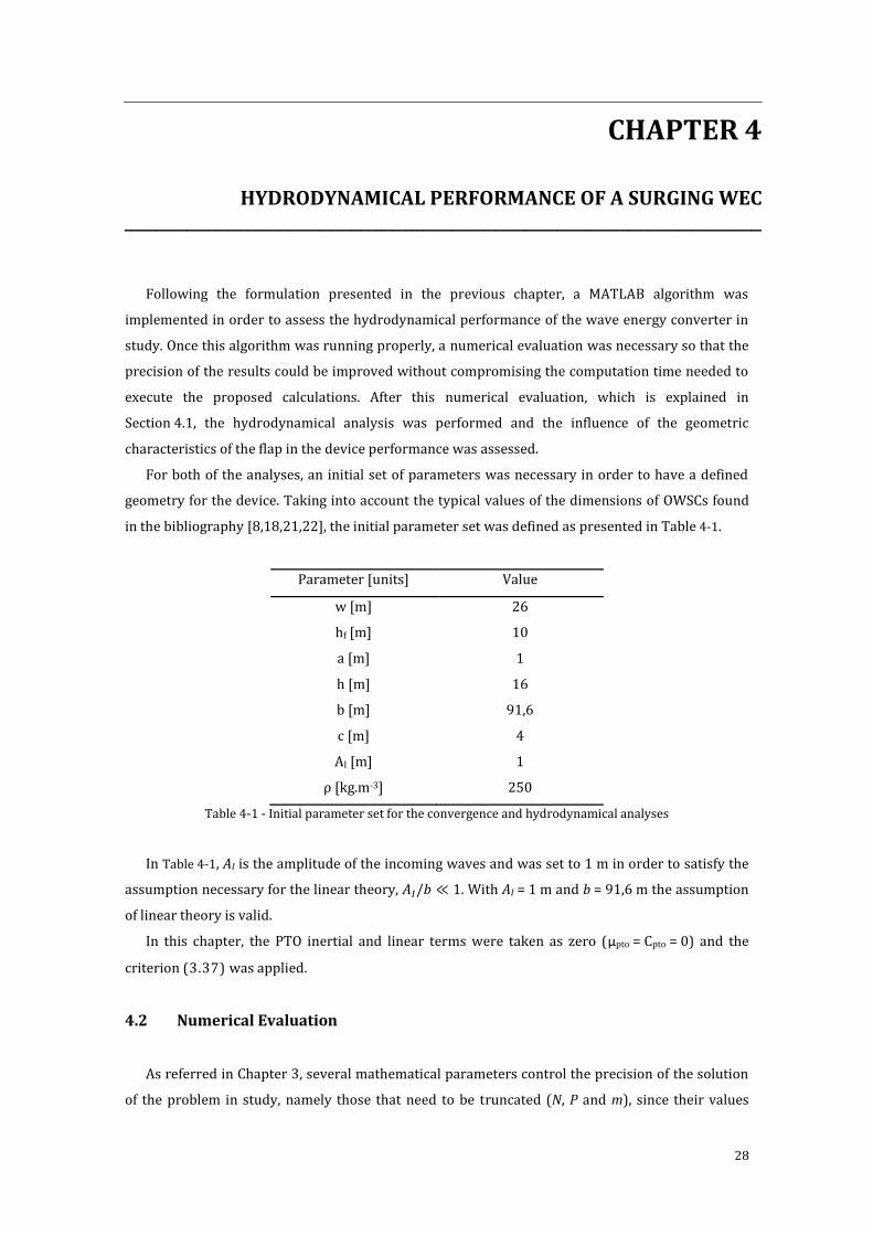
For both of the analyses, an initial set of parameters was necessary in order to have a defined

geometry for the device. Taking into account the typical values of the dimensions of OWSCs found

in the bibliography [8,18,21,22], the initial parameter set was defined as presented in Table 4-1.

Parameter [units] Value

w [m] 26

hf [m] 10

a [m] 1

h [m] 16

b [m] 91,6

c [m] 4

AI [m] 1

ρ [kg.m-3] 250

Table 4-1 - Initial parameter set for the convergence and hydrodynamical analyses

In Table 4-1, AI is the amplitude of the incoming waves and was set to 1 m in order to satisfy the

assumption necessary for the linear theory, 𝐴𝐼/𝑏 ≪ 1. With AI = 1 m and b = 91,6 m the assumption

of linear theory is valid.

In this chapter, the PTO inertial and linear terms were taken as zero (μpto = Cpto = 0) and the

criterion (3.37) was applied.

4.2 Numerical Evaluation

As referred in Chapter 3, several mathematical parameters control the precision of the solution

of the problem in study, namely those that need to be truncated (N, P and m), since their values

29

dictate how far the summations they appear in go. In order to determine the best relation between

precision and computational time required, it was necessary to perform a convergence analysis of

the aforementioned variables, and also for the integration interval of equation (3.24).

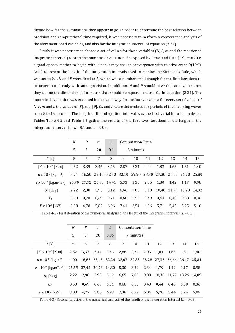
Firstly it was necessary to choose a set of values for these variables (N, P, m and the mentioned

integration interval) to start the numerical evaluation. As exposed by Renzi and Dias [12], m = 20 is

a good approximation to begin with, since it may ensure convergence with relative error O(10-3).

Let L represent the length of the integration intervals used to employ the Simpson’s Rule, which

was set to 0,1. N and P were fixed to 5, which was a number small enough for the first iterations to

be faster, but already with some precision. In addition, N and P should have the same value since

they define the dimensions of a matrix that should be square – matrix Cpn in equation (3.24). The

numerical evaluation was executed in the same way for the four variables: for every set of values of

N, P, m and L the values of |F|, μ, ν, |Θ|, CF, and P were determined for periods of the incoming waves

from 5 to 15 seconds. The length of the integration interval was the first variable to be analysed.

Tables Table 4-2 and Table 4-3 gather the results of the first two iterations of the length of the

integration interval, for L = 0,1 and L = 0,05.

N P m L Computation Time

5 5 20 0,1 3 minutes

T [s] 5 6 7 8 9 10 11 12 13 14 15

|F| x 10-7 [N.m] 2,52 3,39 3,46 3,45 2,87 2,34 2,04 1,82 1,65 1,51 1,40

μ x 10-7 [kg.m2] 3,74 16,50 25,40 32,30 33,10 29,90 28,30 27,30 26,60 26,20 25,80

ν x 10-7 [kg.m2.s-1] 25,70 27,72 20,98 14,41 5,33 3,30 2,35 1,80 1,42 1,17 0,98

|Θ| [deg] 2,22 2,98 3,95 5,12 6,66 7,86 9,10 10,40 11,79 13,29 14,92

CF 0,58 0,70 0,69 0,71 0,68 0,56 0,49 0,44 0,40 0,38 0,36

P x 10-2 [kW] 3,08 4,78 5,82 6,96 7,41 6,54 6,06 5,71 5,45 5,25 5,10

Table 4-2 - First iteration of the numerical analysis of the length of the integration intervals (L = 0,1)

N P m L Computation Time

5 5 20 0.05 7 minutes

T [s] 5 6 7 8 9 10 11 12 13 14 15

|F| x 10-7 [N.m] 2,52 3,37 3,44 3,43 2,86 2,34 2,03 1,81 1,65 1,51 1,40

μ x 10-7 [kg.m2] 4,00 16,62 25,45 32,26 33,07 29,83 28,28 27,32 26,66 26,17 25,81

ν x 10-7 [kg.m2.s-1] 25,59 27,45 20,78 14,30 5,30 3,29 2,34 1,79 1,42 1,17 0,98

|Θ| [deg] 2,22 2,98 3,95 5,12 6,65 7,85 9,08 10,38 11,77 13,26 14,89

CF 0,58 0,69 0,69 0,71 0,68 0,55 0,48 0,44 0,40 0,38 0,36

P x 10-2 [kW] 3,08 4,77 5,80 6,93 7,38 6,52 6,04 5,70 5,44 5,24 5,09

Table 4-3 - Second iteration of the numerical analysis of the length of the integration Interval (L = 0,05)

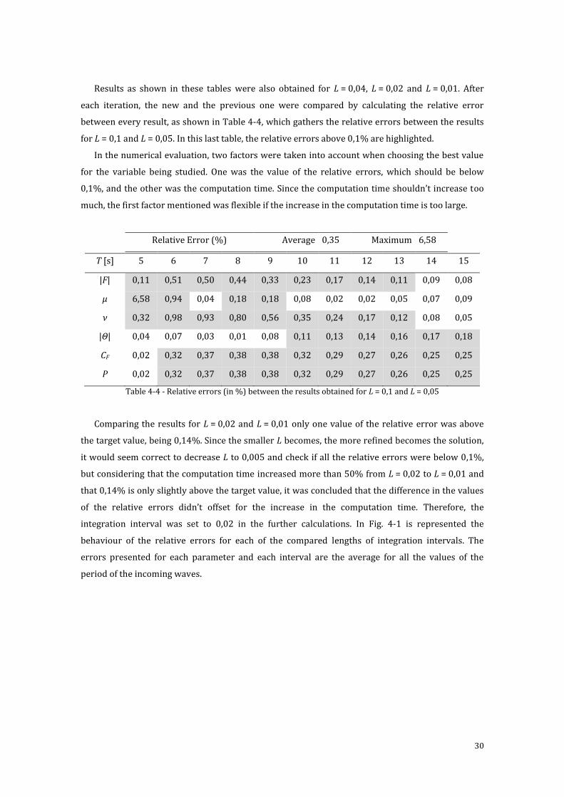
30

Results as shown in these tables were also obtained for L = 0,04, L = 0,02 and L = 0,01. After

each iteration, the new and the previous one were compared by calculating the relative error

between every result, as shown in Table 4-4, which gathers the relative errors between the results

for L = 0,1 and L = 0,05. In this last table, the relative errors above 0,1% are highlighted.

In the numerical evaluation, two factors were taken into account when choosing the best value

for the variable being studied. One was the value of the relative errors, which should be below

0,1%, and the other was the computation time. Since the computation time shouldn’t increase too

much, the first factor mentioned was flexible if the increase in the computation time is too large.

Relative Error (%) Average 0,35 Maximum 6,58

T [s] 5 6 7 8 9 10 11 12 13 14 15

|F| 0,11 0,51 0,50 0,44 0,33 0,23 0,17 0,14 0,11 0,09 0,08

μ 6,58 0,94 0,04 0,18 0,18 0,08 0,02 0,02 0,05 0,07 0,09

ν 0,32 0,98 0,93 0,80 0,56 0,35 0,24 0,17 0,12 0,08 0,05

|Θ| 0,04 0,07 0,03 0,01 0,08 0,11 0,13 0,14 0,16 0,17 0,18

CF 0,02 0,32 0,37 0,38 0,38 0,32 0,29 0,27 0,26 0,25 0,25

P 0,02 0,32 0,37 0,38 0,38 0,32 0,29 0,27 0,26 0,25 0,25

Table 4-4 - Relative errors (in %) between the results obtained for L = 0,1 and L = 0,05

Comparing the results for L = 0,02 and L = 0,01 only one value of the relative error was above

the target value, being 0,14%. Since the smaller L becomes, the more refined becomes the solution,

it would seem correct to decrease L to 0,005 and check if all the relative errors were below 0,1%,

but considering that the computation time increased more than 50% from L = 0,02 to L = 0,01 and

that 0,14% is only slightly above the target value, it was concluded that the difference in the values

of the relative errors didn’t offset for the increase in the computation time. Therefore, the

integration interval was set to 0,02 in the further calculations. In Fig. 4-1 is represented the

behaviour of the relative errors for each of the compared lengths of integration intervals. The

errors presented for each parameter and each interval are the average for all the values of the

period of the incoming waves.

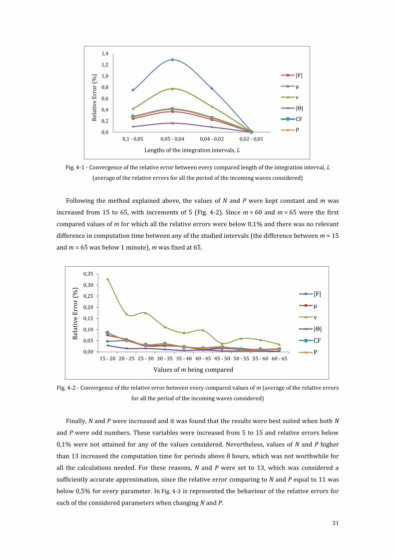
31

Fig. 4-1 - Convergence of the relative error between every compared length of the integration interval, L

(average of the relative errors for all the period of the incoming waves considered)

Following the method explained above, the values of N and P were kept constant and m was

increased from 15 to 65, with increments of 5 (Fig. 4-2). Since m = 60 and m = 65 were the first

compared values of m for which all the relative errors were below 0,1% and there was no relevant

difference in computation time between any of the studied intervals (the difference between m = 15

and m = 65 was below 1 minute), m was fixed at 65.

Fig. 4-2 - Convergence of the relative error between every compared values of m (average of the relative errors

for all the period of the incoming waves considered)

Finally, N and P were increased and it was found that the results were best suited when both N

and P were odd numbers. These variables were increased from 5 to 15 and relative errors below

0,1% were not attained for any of the values considered. Nevertheless, values of N and P higher

than 13 increased the computation time for periods above 8 hours, which was not worthwhile for

all the calculations needed. For these reasons, N and P were set to 13, which was considered a

sufficiently accurate approximation, since the relative error comparing to N and P equal to 11 was

below 0,5% for every parameter. In Fig. 4-3 is represented the behaviour of the relative errors for

each of the considered parameters when changing N and P.

0,0

0,2

0,4

0,6

0,8

1,0

1,2

1,4

0,1 - 0,05 0,05 - 0,04 0,04 - 0,02 0,02 - 0,01

Rel

ativ

e E

rro

r (%

)

Lengths of the integration intervals, L

|F|

μ

ν

|Θ|

CF

P

0,00

0,05

0,10

0,15

0,20

0,25

0,30

0,35

15 - 20 20 - 25 25 - 30 30 - 35 35 - 40 40 - 45 45 - 50 50 - 55 55 - 60 60 - 65

Rel

ativ

e E

rro

r (%

)

Values of m being compared

|F|

μ

ν

|Θ|

CF

P

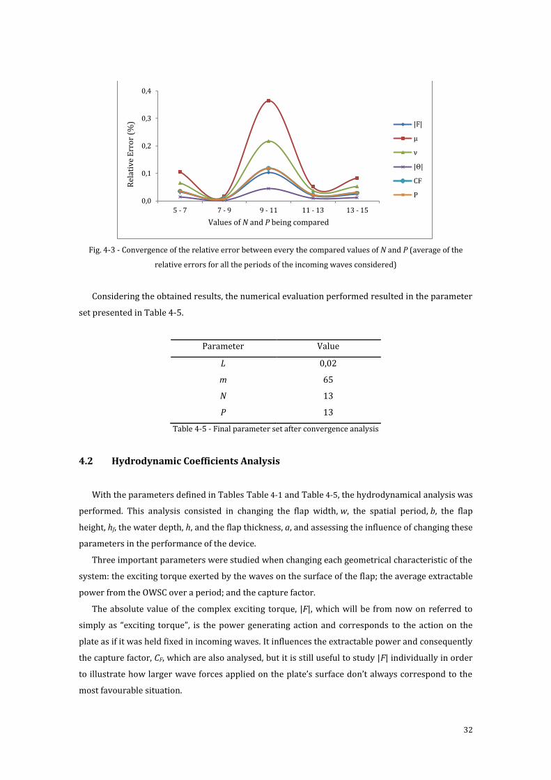
32

Fig. 4-3 - Convergence of the relative error between every the compared values of N and P (average of the

relative errors for all the periods of the incoming waves considered)

Considering the obtained results, the numerical evaluation performed resulted in the parameter

set presented in Table 4-5.

Parameter Value

L 0,02

m 65

N 13

P 13

Table 4-5 - Final parameter set after convergence analysis

4.2 Hydrodynamic Coefficients Analysis

With the parameters defined in Tables Table 4-1 and Table 4-5, the hydrodynamical analysis was

performed. This analysis consisted in changing the flap width, w, the spatial period, b, the flap

height, hf, the water depth, h, and the flap thickness, a, and assessing the influence of changing these

parameters in the performance of the device.

Three important parameters were studied when changing each geometrical characteristic of the

system: the exciting torque exerted by the waves on the surface of the flap; the average extractable

power from the OWSC over a period; and the capture factor.

The absolute value of the complex exciting torque, |F|, which will be from now on referred to

simply as “exciting torque”, is the power generating action and corresponds to the action on the

plate as if it was held fixed in incoming waves. It influences the extractable power and consequently

the capture factor, CF, which are also analysed, but it is still useful to study |F| individually in order

to illustrate how larger wave forces applied on the plate’s surface don’t always correspond to the

most favourable situation.

0,0

0,1

0,2

0,3

0,4

5 - 7 7 - 9 9 - 11 11 - 13 13 - 15

Rel

ativ

e E

rro

r (%

)

Values of N and P being compared

|F|

μ

ν

|Θ|

CF

P

33

The capture factor allows an efficiency assessment and it is defined as the ratio between the

extractable power per unit flap width and the power of the incident wave field per unit crest length,

i.e. it shows how much of the available power per unit length of a wave is being actually extracted

by the device, which is the third parameter analysed - the average extracted power from the OWSC

over a period, P. Naturally, this extracted power is not the final power available for consumption,

since it still suffers losses due to different factors, such as friction between parts of the system,

viscosity, transportation through the pipes and losses intrinsic to the electrical generator. It is also

subjected to the capacity of the PTO system, which might not be higher enough to convert all the

power P made available by the movement of the flap.

For each change in every set of geometrical characteristics studied, the problem in Section 3.2

was solved in order to determine the values of |F|, P and CF. In this chapter, the optimising criterion

for the rate of power take-off was applied, such that 𝜈𝑝𝑡𝑜 = 𝜈𝑜𝑝𝑡 , and the PTO inertial and linear

terms were considered equal to 0.

4.2.1 Flap width, w

The first influencing parameter to be studied was the width of the flap, being this the dimension

parallel to the seabed, to the shoreline and to most of the incoming waves (Fig. 3-1).

For every value of the width that was considered, from 14 m to 30 m with increments of 4 m, the

corresponding values of the absolute complex exciting torque, |F|, capture factor, CF, and captured

power, P, were determined for periods of the incoming waves from 5 s to 15 s, similarly to what

was made for the convergence analysis.

Increasing the width of the flap corresponds to increasing the surface area exposed to the

incoming waves. Consequently, a larger width determines higher inertia torque and exciting torque,

as stated in equations (3.17) and (3.19), for which it was expected a general increase in |F| for

wider flaps. This was verified by the obtained results, as illustrated in Fig. 4-4.

It was also noted that the maximum value of |F| increases with the width and occurs for higher

periods of the incident waves. For lower values of the period T, the torque increases less and less

with the increasing width, as illustrated in Fig. 4-4. For instance, for T = 5 s, the difference between

the values of the complex exciting torque for w = 14 m and w = 18 m is visible on the plot

(approx. 15%), while the same difference for w = 30 m and w = 26 m is almost imperceptible

(approx. 6%).

Since the power is proportional to the square of |F|, it was also expected that the power

absorbed increased with the flap width, as well as the capture factor which depends on the

extracted power. These results are illustrated in Fig. 4-5 and Fig. 4-6.

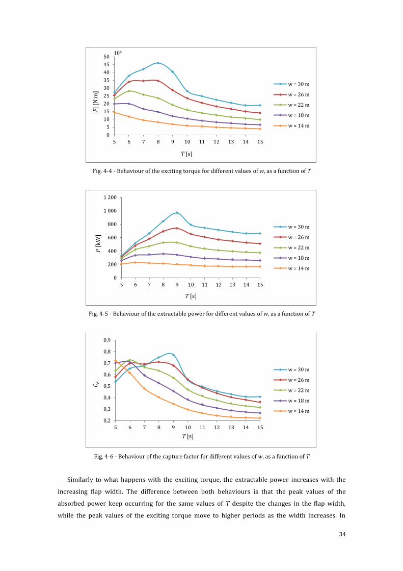
34

Fig. 4-4 - Behaviour of the exciting torque for different values of w, as a function of T

Fig. 4-5 - Behaviour of the extractable power for different values of w, as a function of T

Fig. 4-6 - Behaviour of the capture factor for different values of w, as a function of T

Similarly to what happens with the exciting torque, the extractable power increases with the

increasing flap width. The difference between both behaviours is that the peak values of the

absorbed power keep occurring for the same values of T despite the changes in the flap width,

while the peak values of the exciting torque move to higher periods as the width increases. In

0

5

10

15

20

25

30

35

40

45

50

5 6 7 8 9 10 11 12 13 14 15

|F|

[N.m

]

T [s]

w = 30 m

w = 26 m

w = 22 m

w = 18 m

w = 14 m

106

0

200

400

600

800

1 000

1 200

5 6 7 8 9 10 11 12 13 14 15

P [

kW

]

T [s]

w = 30 m

w = 26 m

w = 22 m

w = 18 m

w = 14 m

0,2

0,3

0,4

0,5

0,6

0,7

0,8

0,9

5 6 7 8 9 10 11 12 13 14 15

CF

T [s]

w = 30 m

w = 26 m

w = 22 m

w = 18 m

w = 14 m

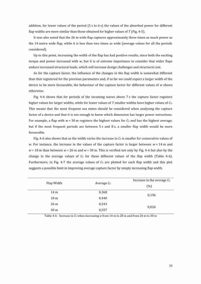
35

addition, for lower values of the period (5 s to 6 s) the values of the absorbed power for different

flap widths are more similar than those obtained for higher values of T (Fig. 4-5).

It was also noted that the 26 m wide flap captures approximately three times as much power as

the 14 metre wide flap, while it is less than two times as wide (average values for all the periods

considered).

Up to this point, increasing the width of the flap has had positive results, since both the exciting

torque and power increased with w, but it is of extreme importance to consider that wider flaps

endure increased structural loads, which will increase design challenges and structural cost.

As for the capture factor, the influence of the changes in the flap width is somewhat different

than that registered for the previous parameters and, if so far we could expect a larger width of the

device to be more favourable, the behaviour of the capture factor for different values of w shows

otherwise.

Fig. 4-6 shows that for periods of the incoming waves above 7 s the capture factor registers

higher values for larger widths, while for lower values of T smaller widths have higher values of CF.

This means that the most frequent sea states should be considered when analysing the capture

factor of a device and that it is not enough to know which dimension has larger power extractions.

For example, a flap with w = 30 m registers the highest values for CF and has the highest average;

but if the most frequent periods are between 5 s and 8 s, a smaller flap width would be more

favourable.

Fig. 4-6 also shows that as the width varies the increase in CF is smaller for consecutive values of

w. For instance, the increase in the values of the capture factor is larger between w = 14 m and

w = 18 m than between w = 26 m and w = 30 m. This is verified not only by Fig. 4-6 but also by the

change in the average values of CF for these different values of the flap width (Table 4-6).

Furthermore, in Fig. 4-7 the average values of CF are plotted for each flap width and this plot

suggests a possible limit in improving average capture factor by simply increasing flap width.

Flap Width Average CF Increase in the average CF

(%)

14 m 0,368 0,196

18 m 0,440

26 m 0,543 0,026

30 m 0,557

Table 4-6 - Increase in CF when increasing w from 14 m to 28 m and from 26 m to 30 m

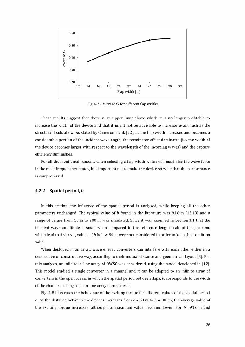
36

Fig. 4-7 - Average CF for different flap widths

These results suggest that there is an upper limit above which it is no longer profitable to

increase the width of the device and that it might not be advisable to increase w as much as the

structural loads allow. As stated by Cameron et. al. [22], as the flap width increases and becomes a

considerable portion of the incident wavelength, the terminator effect dominates (i.e. the width of

the device becomes larger with respect to the wavelength of the incoming waves) and the capture

efficiency diminishes.

For all the mentioned reasons, when selecting a flap width which will maximise the wave force

in the most frequent sea states, it is important not to make the device so wide that the performance

is compromised.

4.2.2 Spatial period, b

In this section, the influence of the spatial period is analysed, while keeping all the other

parameters unchanged. The typical value of b found in the literature was 91,6 m [12,18] and a

range of values from 50 m to 200 m was simulated. Since it was assumed in Section 3.1 that the

incident wave amplitude is small when compared to the reference length scale of the problem,

which lead to A/b << 1, values of b below 50 m were not considered in order to keep this condition

valid.

When deployed in an array, wave energy converters can interfere with each other either in a

destructive or constructive way, according to their mutual distance and geometrical layout [8]. For

this analysis, an infinite in-line array of OWSC was considered, using the model developed in [12].

This model studied a single converter in a channel and it can be adapted to an infinite array of

converters in the open ocean, in which the spatial period between flaps, b, corresponds to the width

of the channel, as long as an in-line array is considered.

Fig. 4-8 illustrates the behaviour of the exciting torque for different values of the spatial period

b. As the distance between the devices increases from b = 50 m to b = 100 m, the average value of

the exciting torque increases, although its maximum value becomes lower. For b = 91,6 m and

0,20

0,30

0,40

0,50

0,60

12 14 16 18 20 22 24 26 28 30 32

Av

erag

e C

F

Flap width [m]

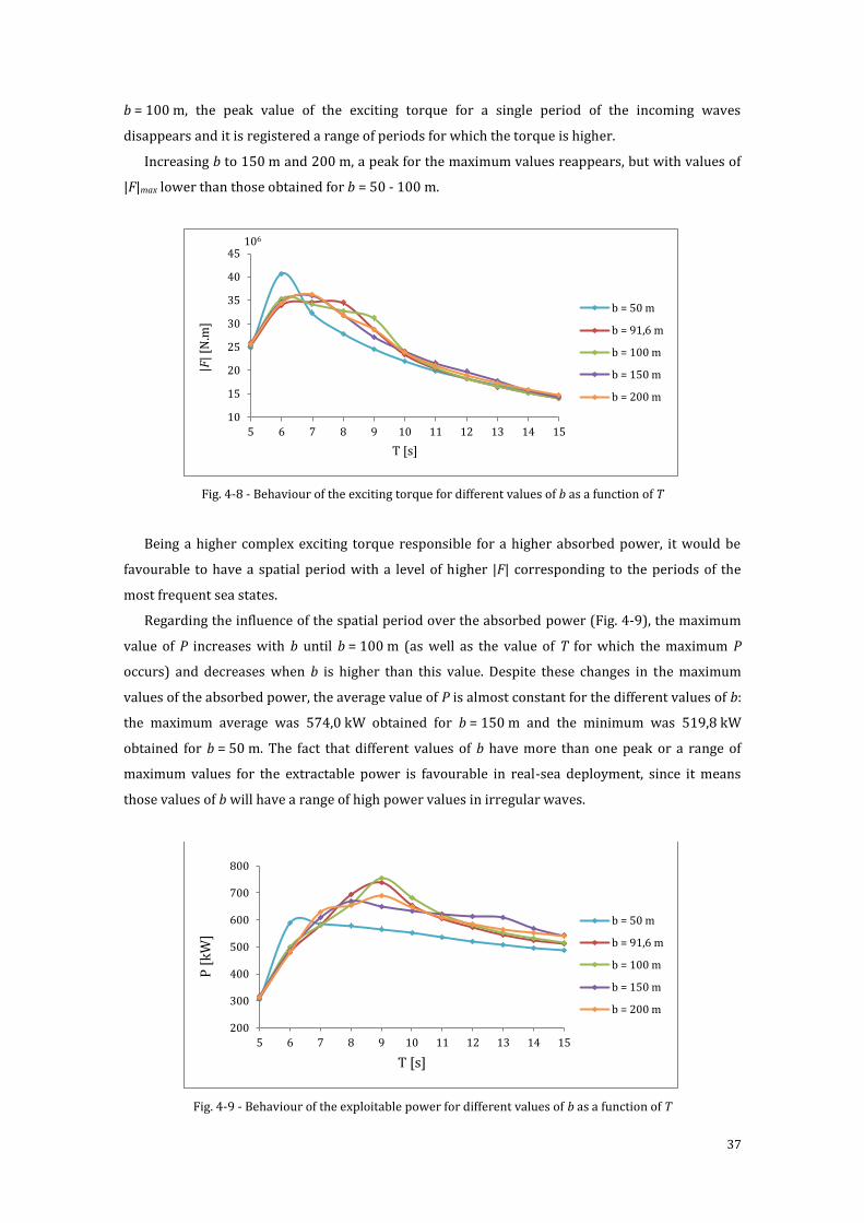
37

b = 100 m, the peak value of the exciting torque for a single period of the incoming waves

disappears and it is registered a range of periods for which the torque is higher.

Increasing b to 150 m and 200 m, a peak for the maximum values reappears, but with values of

|F|max lower than those obtained for b = 50 - 100 m.

Fig. 4-8 - Behaviour of the exciting torque for different values of b as a function of T

Being a higher complex exciting torque responsible for a higher absorbed power, it would be

favourable to have a spatial period with a level of higher |F| corresponding to the periods of the

most frequent sea states.

Regarding the influence of the spatial period over the absorbed power (Fig. 4-9), the maximum

value of P increases with b until b = 100 m (as well as the value of T for which the maximum P

occurs) and decreases when b is higher than this value. Despite these changes in the maximum

values of the absorbed power, the average value of P is almost constant for the different values of b:

the maximum average was 574,0 kW obtained for b = 150 m and the minimum was 519,8 kW

obtained for b = 50 m. The fact that different values of b have more than one peak or a range of

maximum values for the extractable power is favourable in real-sea deployment, since it means

those values of b will have a range of high power values in irregular waves.

Fig. 4-9 - Behaviour of the exploitable power for different values of b as a function of T

10

15

20

25

30

35

40

45

5 6 7 8 9 10 11 12 13 14 15

|F|

[N.m

]

T [s]

b = 50 m

b = 91,6 m

b = 100 m

b = 150 m

b = 200 m

106

200

300

400

500

600

700

800

5 6 7 8 9 10 11 12 13 14 15

P [

kW

]

T [s]

b = 50 m

b = 91,6 m

b = 100 m

b = 150 m

b = 200 m

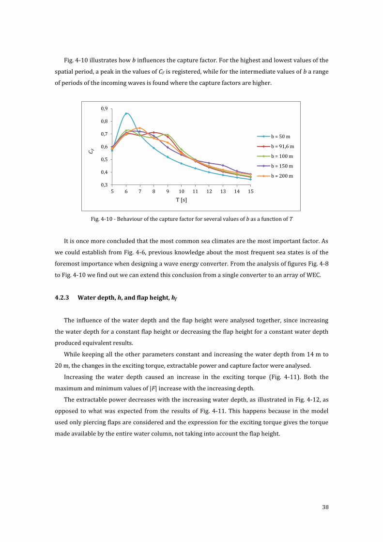
38

Fig. 4-10 illustrates how b influences the capture factor. For the highest and lowest values of the

spatial period, a peak in the values of CF is registered, while for the intermediate values of b a range

of periods of the incoming waves is found where the capture factors are higher.

Fig. 4-10 - Behaviour of the capture factor for several values of b as a function of T

It is once more concluded that the most common sea climates are the most important factor. As

we could establish from Fig. 4-6, previous knowledge about the most frequent sea states is of the

foremost importance when designing a wave energy converter. From the analysis of figures Fig. 4-8

to Fig. 4-10 we find out we can extend this conclusion from a single converter to an array of WEC.

4.2.3 Water depth, h, and flap height, hf

The influence of the water depth and the flap height were analysed together, since increasing

the water depth for a constant flap height or decreasing the flap height for a constant water depth

produced equivalent results.

While keeping all the other parameters constant and increasing the water depth from 14 m to

20 m, the changes in the exciting torque, extractable power and capture factor were analysed.

Increasing the water depth caused an increase in the exciting torque (Fig. 4-11). Both the

maximum and minimum values of |F| increase with the increasing depth.

The extractable power decreases with the increasing water depth, as illustrated in Fig. 4-12, as

opposed to what was expected from the results of Fig. 4-11. This happens because in the model

used only piercing flaps are considered and the expression for the exciting torque gives the torque

made available by the entire water column, not taking into account the flap height.

0,3

0,4

0,5

0,6

0,7

0,8

0,9

5 6 7 8 9 10 11 12 13 14 15

CF

T [s]

b = 50 m

b = 91,6 m

b = 100 m

b = 150 m

b = 200 m

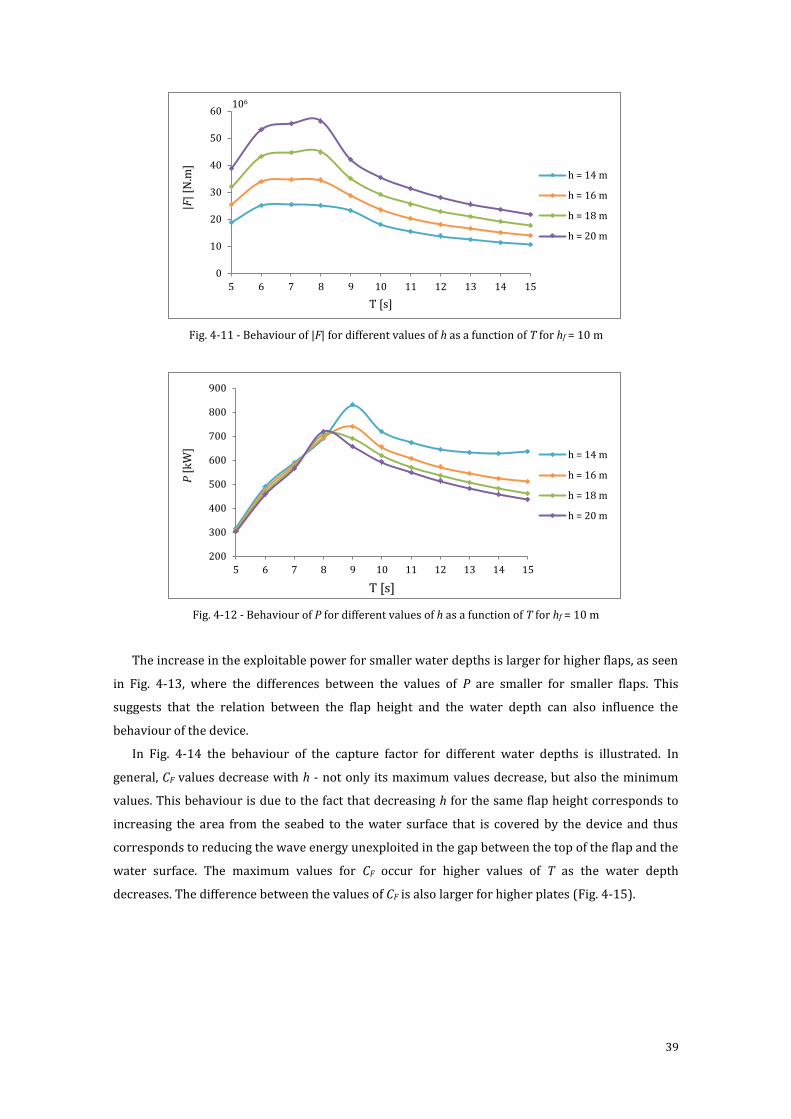
39

Fig. 4-11 - Behaviour of |F| for different values of h as a function of T for hf = 10 m

Fig. 4-12 - Behaviour of P for different values of h as a function of T for hf = 10 m

The increase in the exploitable power for smaller water depths is larger for higher flaps, as seen

in Fig. 4-13, where the differences between the values of P are smaller for smaller flaps. This

suggests that the relation between the flap height and the water depth can also influence the

behaviour of the device.

In Fig. 4-14 the behaviour of the capture factor for different water depths is illustrated. In

general, CF values decrease with h - not only its maximum values decrease, but also the minimum

values. This behaviour is due to the fact that decreasing h for the same flap height corresponds to

increasing the area from the seabed to the water surface that is covered by the device and thus

corresponds to reducing the wave energy unexploited in the gap between the top of the flap and the

water surface. The maximum values for CF occur for higher values of T as the water depth

decreases. The difference between the values of CF is also larger for higher plates (Fig. 4-15).

0

10

20

30

40

50

60

5 6 7 8 9 10 11 12 13 14 15

|F|

[N.m

]

T [s]

h = 14 m

h = 16 m

h = 18 m

h = 20 m

106

200

300

400

500

600

700

800

900

5 6 7 8 9 10 11 12 13 14 15

P [

kW

]

T [s]

h = 14 m

h = 16 m

h = 18 m

h = 20 m

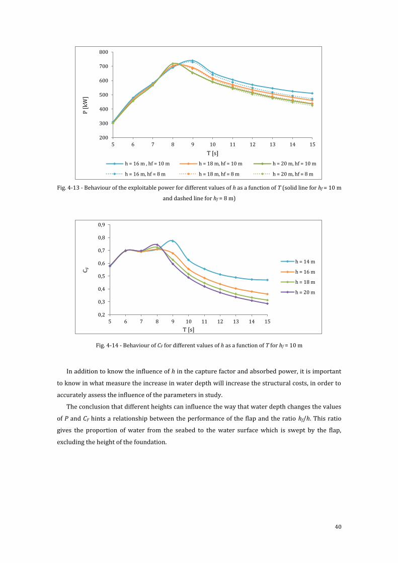
40

Fig. 4-13 - Behaviour of the exploitable power for different values of h as a function of T (solid line for hf = 10 m

and dashed line for hf = 8 m)

Fig. 4-14 - Behaviour of CF for different values of h as a function of T for hf = 10 m

In addition to know the influence of h in the capture factor and absorbed power, it is important

to know in what measure the increase in water depth will increase the structural costs, in order to

accurately assess the influence of the parameters in study.

The conclusion that different heights can influence the way that water depth changes the values

of P and CF hints a relationship between the performance of the flap and the ratio hf/h. This ratio

gives the proportion of water from the seabed to the water surface which is swept by the flap,

excluding the height of the foundation.

200

300

400

500

600

700

800

5 6 7 8 9 10 11 12 13 14 15

P [

kW

]

T [s]

h = 16 m , hf = 10 m h = 18 m, hf = 10 m h = 20 m, hf = 10 m

h = 16 m, hf = 8 m h = 18 m, hf = 8 m h = 20 m, hf = 8 m

0,2

0,3

0,4

0,5

0,6

0,7

0,8

0,9

5 6 7 8 9 10 11 12 13 14 15

CF

T [s]

h = 14 m

h = 16 m

h = 18 m

h = 20 m

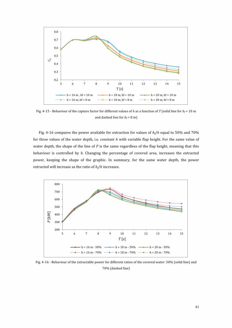
41

Fig. 4-15 - Behaviour of the capture factor for different values of h as a function of T (solid line for hf = 10 m

and dashed line for hf = 8 m)

Fig. 4-16 compares the power available for extraction for values of hf/h equal to 50% and 70%

for three values of the water depth, i.e. constant h with variable flap height. For the same value of

water depth, the shape of the line of P is the same regardless of the flap height, meaning that this

behaviour is controlled by h. Changing the percentage of covered area, increases the extracted

power, keeping the shape of the graphic. In summary, for the same water depth, the power

extracted will increase as the ratio of hf/h increases.

Fig. 4-16 - Behaviour of the extractable power for different ratios of the covered water: 50% (solid line) and

70% (dashed line)

0,2

0,3

0,4

0,5

0,6

0,7

0,8

5 6 7 8 9 10 11 12 13 14 15

CF

T [s]

h = 16 m , hf = 10 m h = 18 m, hf = 10 m h = 20 m, hf = 10 m

h = 16 m, hf = 8 m h = 18 m, hf = 8 m h = 20 m, hf = 8 m

200

300

400

500

600

700

800

5 6 7 8 9 10 11 12 13 14 15

P [

kW

]

T [s]

h = 16 m - 50% h = 18 m - 50% h = 20 m - 50%

h = 16 m - 70% h = 18 m - 70% h = 20 m - 70%

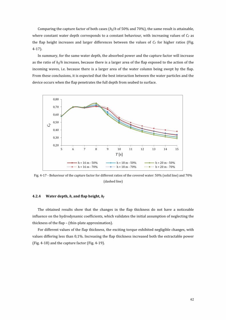
42

Comparing the capture factor of both cases (hf/h of 50% and 70%), the same result is attainable,

where constant water depth corresponds to a constant behaviour, with increasing values of CF as

the flap height increases and larger differences between the values of CF for higher ratios (Fig.

4-17).

In summary, for the same water depth, the absorbed power and the capture factor will increase

as the ratio of hf/h increases, because there is a larger area of the flap exposed to the action of the

incoming waves, i.e. because there is a larger area of the water column being swept by the flap.

From these conclusions, it is expected that the best interaction between the water particles and the

device occurs when the flap penetrates the full depth from seabed to surface.

Fig. 4-17 - Behaviour of the capture factor for different ratios of the covered water: 50% (solid line) and 70%

(dashed line)

4.2.4 Water depth, h, and flap height, hf

The obtained results show that the changes in the flap thickness do not have a noticeable

influence on the hydrodynamic coefficients, which validates the initial assumption of neglecting the

thickness of the flap – (thin-plate approximation).

For different values of the flap thickness, the exciting torque exhibited negligible changes, with

values differing less than 0,1%. Increasing the flap thickness increased both the extractable power

(Fig. 4-18) and the capture factor (Fig. 4-19).

0,20

0,30

0,40

0,50

0,60

0,70

0,80

5 6 7 8 9 10 11 12 13 14 15

CF

T [s]

h = 16 m - 50% h = 18 m - 50% h = 20 m - 50%

h = 16 m - 70% h = 18 m - 70% h = 20 m - 70%

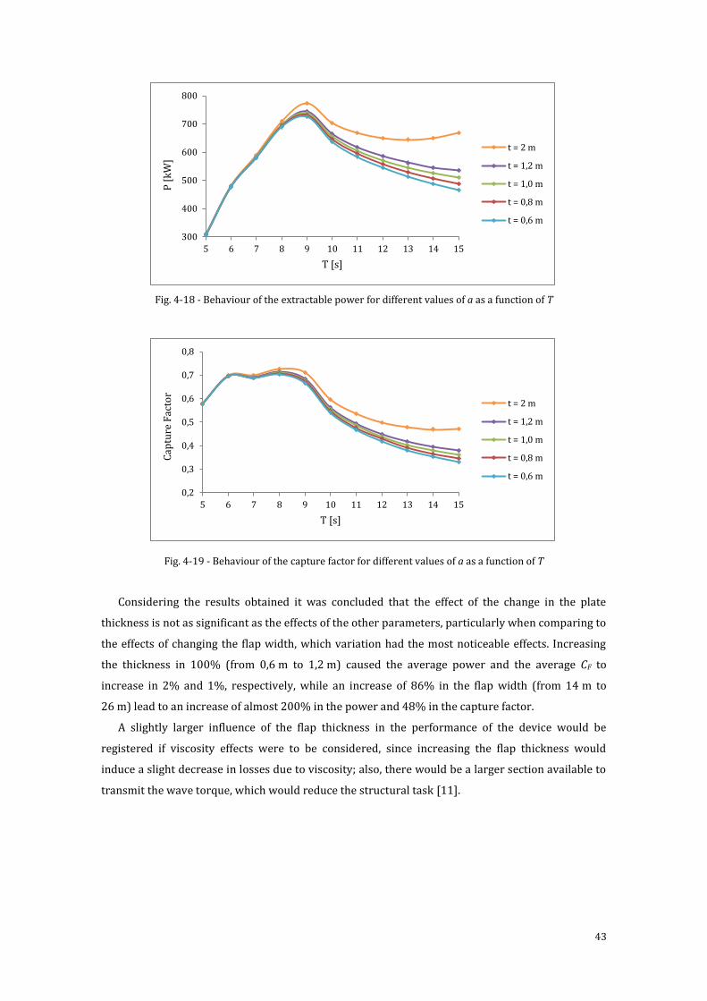
43

Fig. 4-18 - Behaviour of the extractable power for different values of a as a function of T

Fig. 4-19 - Behaviour of the capture factor for different values of a as a function of T

Considering the results obtained it was concluded that the effect of the change in the plate

thickness is not as significant as the effects of the other parameters, particularly when comparing to

the effects of changing the flap width, which variation had the most noticeable effects. Increasing

the thickness in 100% (from 0,6 m to 1,2 m) caused the average power and the average CF to

increase in 2% and 1%, respectively, while an increase of 86% in the flap width (from 14 m to

26 m) lead to an increase of almost 200% in the power and 48% in the capture factor.

A slightly larger influence of the flap thickness in the performance of the device would be

registered if viscosity effects were to be considered, since increasing the flap thickness would

induce a slight decrease in losses due to viscosity; also, there would be a larger section available to

transmit the wave torque, which would reduce the structural task [11].

300

400

500

600

700

800

5 6 7 8 9 10 11 12 13 14 15

P [

kW

]

T [s]

t = 2 m

t = 1,2 m

t = 1,0 m

t = 0,8 m

t = 0,6 m

0,2

0,3

0,4

0,5

0,6

0,7

0,8

5 6 7 8 9 10 11 12 13 14 15

Cap

ture

Fac

tor

T [s]

t = 2 m

t = 1,2 m

t = 1,0 m

t = 0,8 m

t = 0,6 m

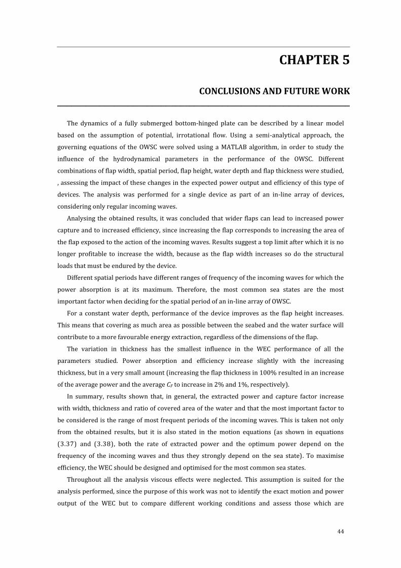
44

5CHAPTER 5

CONCLUSIONS AND FUTURE WORK ______________________________________________________________

The dynamics of a fully submerged bottom-hinged plate can be described by a linear model

based on the assumption of potential, irrotational flow. Using a semi-analytical approach, the

governing equations of the OWSC were solved using a MATLAB algorithm, in order to study the

influence of the hydrodynamical parameters in the performance of the OWSC. Different

combinations of flap width, spatial period, flap height, water depth and flap thickness were studied,

, assessing the impact of these changes in the expected power output and efficiency of this type of

devices. The analysis was performed for a single device as part of an in-line array of devices,

considering only regular incoming waves.

Analysing the obtained results, it was concluded that wider flaps can lead to increased power

capture and to increased efficiency, since increasing the flap corresponds to increasing the area of

the flap exposed to the action of the incoming waves. Results suggest a top limit after which it is no

longer profitable to increase the width, because as the flap width increases so do the structural

loads that must be endured by the device.

Different spatial periods have different ranges of frequency of the incoming waves for which the

power absorption is at its maximum. Therefore, the most common sea states are the most

important factor when deciding for the spatial period of an in-line array of OWSC.

For a constant water depth, performance of the device improves as the flap height increases.

This means that covering as much area as possible between the seabed and the water surface will

contribute to a more favourable energy extraction, regardless of the dimensions of the flap.

The variation in thickness has the smallest influence in the WEC performance of all the

parameters studied. Power absorption and efficiency increase slightly with the increasing

thickness, but in a very small amount (increasing the flap thickness in 100% resulted in an increase

of the average power and the average CF to increase in 2% and 1%, respectively).

In summary, results shown that, in general, the extracted power and capture factor increase

with width, thickness and ratio of covered area of the water and that the most important factor to

be considered is the range of most frequent periods of the incoming waves. This is taken not only

from the obtained results, but it is also stated in the motion equations (as shown in equations

(3.37) and (3.38), both the rate of extracted power and the optimum power depend on the

frequency of the incoming waves and thus they strongly depend on the sea state). To maximise

efficiency, the WEC should be designed and optimised for the most common sea states.

Throughout all the analysis viscous effects were neglected. This assumption is suited for the

analysis performed, since the purpose of this work was not to identify the exact motion and power

output of the WEC but to compare different working conditions and assess those which are

45

favourable to improving the device performance. By including the effects of viscosity in the

analysis, losses would be expected to have a significant effect on the system behaviour.

During the analysis incident waves were assumed to be harmonic and monochromatic. This

approximation is appropriate, since irregular waves can be considered as a superposition of regular

waves and therefore the dynamics of the system would still be governed by the same mechanisms

and the present analysis remains valid when considering deployment in a real environment, where

waves are irregular.

The evaluation performed was restricted to regular waves and inviscid fluid and its simplicity

makes it unattainable to evaluate the interaction of all the parameters simultaneously.

Nevertheless, it illustrates important relations and leads to insightful conclusions, helpful in

improving the design of OWSCs.

The performed analysis can be improved in several ways with further investigation. In addition

to the studied parameters, inclusion of irregular waves in the analysis would be of most interest,

since it would allow studying the influence of different sea states and an optimal device

configuration could be established for different wave climate combinations. Investigation would

also be improved by considering the behaviour of the angular displacement in the analysis as it was

made for the exciting torque, extractable power and capture factor.

Including viscous effects and their variation with body shape would be useful in a more accurate

power extraction forecast and in improving the shape of the device. Also, further adaptation of the

model to fully submerged OWSCs is necessary, namely by adding one additional boundary

condition relative to the tip of the flap. Finally, combining the capture factor with other

performance assessment factors would allow a deeper insight over the parameters influencing the

behaviour of the converter studied.

46

REFERENCES

______________________________________________________________

[1] Mofor, L., Goldsmith, J., & Jones, F. (2014). Ocean Energy: Technology readiness, patents,

deployment status and outlook. International Renewable Energy Agency.

[2] Magagna, D., & Uihlein, A. (2015). 2014 JRC Ocean Energy Status Report. Publications Office

of the European Union.

[3] REN21 Renewable Energy Policy Network for the 21st Century: http://www.ren21.net/.

(access date May 11, 2016).

[4] AW-Energy: http://aw-energy.com (access dat April 18, 2016).

[5] Lewis, A., Estefen, S., Musial, W., Pontes, T., & Torres-Martinez, J. (2011). Ocean Energy. IPCC

Special Report on Renewable Energy Sources and Climate Change Mitigation, pp. 497-533.

[6] The European Marine Energy Centre: http://www.emec.org.uk (access date February 25,

2016).

[7] Folley, M., Whittaker, T. J., & Henry, A. (2007). The effect of water depth on the performance

of a small surging wave energy converter. Ocean Engineering, 34, 1265-1274.

[8] Renzi, E., Abdolali, A., Bellotti, G., & Dias, F. (2014). Wave-power absorption from a finite

array of oscillating wave surge converters. Renewable Energy, 63, 55-68.

[9] Pelamis Wave Energy Project.: http://www.eon.com/content/dam/eon-

com/en/downloads/e/E.ON_PELAMIS_INFO_SHEET.pdf (access dat May 9, 2016).

[10] Technology: How Oyster wave power works:

http://www.aquamarinepower.com/technology/how-oyster-wave-power-works.aspx

(access date May 10, 2016).

[11] Folley, M., Whittaker, T., & van't Hoff, J. (2007). The design of small seabed-mounted

bottom-hinged wave energy converters. 7th European Wave and Tidal Energy Conference.

[12] Renzi, E., & Dias, F. (2012). Resonant behaviour of an oscillating wave energy converter in a

channel. Journal of Fluid Mechanics, 701, 482 - 510.

[13] Whittaker, T., Collier, D., Folley, M., Osterried, M., Henry, A., & M., C. (2007). The

development of Oyster - A shallow water surging wave energy converter. 7th European

Wave and Tidal Energy Conference.

[14] Drew, B., Plummer, A. R., & Sahinkaya, M. N. (2009). A review of wave energy converter

technology. Proc. IMechE Part A: J. Power and Energy, 223, 887-902.

[15] Henry, A., Doherty, K., Cameron, L., Whittaker, T., & Doherty, R. (2010). Advances in the

design of Oyster wave energy converter. Marine Renewable and Offshore Wind Energy

Conference. United Kingdom.

[16] Falnes, J. (2002). Ocean Waves and Oscillating Systems. Cambridge University Press.

47

[17] Krogstad, H. E., & Arntsen, O. A. (2000). Linear Wave Theory: Part A - Regular Waves.

Trondheim, Norway: Norwegian University of Science and Technology.

[18] Renzi, E., & Dias, F. (2012). Relations for a periodic array of flap-type wave energy

converters. Applied Ocean Research, 39, 31-39.

[19] Gomes, R., Lopes, M., Henriques, J., Gato, L., & Falcão, A. (2011). A study on the wave energy

conversion by submerged bottom-hinged plates. 9th European Wave and Tidal Energy

Conference.

[20] Mei, C. C., Stiassnie, M., & Yue, D. K. (2005). Theory and Applications of Ocean Surface Waves:

Part 1 Linear Aspects. Singapore: World Scientific Publishing Co. Pte. Ltd.

[21] Renzi, E., & Dias, F. (2013). Hydrodynamics of the oscillating wave surge converter in the

open ocean. European Journal of Mechanics B/ Fluids, 41, 1 - 10.

[22] Cameron, L., Doherty, R., Henry, A., Doherty, K., Van't Hoff, J., Kaye, D., et al. (2010). Design of

the next generation of the Oyster wave energy converter. 3rd International Conference on

Ocean Energy.