Hydrodynamic Object Recognition: When Multipoles Count

Andreas B. Sichert, Robert Bamler, and J. Leo van Hemmen

Physik Department T35 & Bernstein Center for Computational Neuroscience-Munich, Technische Universitat Munchen,85747 Garching bei Munchen, Germany

(Received 21 May 2008; revised manuscript received 15 December 2008; published 6 February 2009)

The lateral-line system is a unique mechanosensory facility of aquatic animals that enables them not

only to localize prey, predator, obstacles, and conspecifics, but also to recognize hydrodynamic objects.

Here we present an explicit model explaining how aquatic animals such as fish can distinguish differently

shaped submerged moving objects. Our model is based on the hydrodynamic multipole expansion and

uses the unambiguous set of multipole components to identify the corresponding object. Furthermore, we

show that within the natural range of one fish length the velocity field contains far more information than

that due to a dipole. Finally, the model we present is easy to implement both neuronally and technically,

and agrees well with available neuronal, physiological, and behavioral data on the lateral-line system.

DOI: 10.1103/PhysRevLett.102.058104 PACS numbers: 87.85.Ng, 47.90.+a, 87.19.lt

All fish and some aquatic amphibians possess a uniquesensory facility, the lateral-line system. This system iscomposed of mechanosensory units called neuromasts lo-cated on the trunk of the animal. They consist of smallcupulae, gelatinous flags protruding into the water, whichare sensitive to the local water velocity [1].

Aquatic animals use their lateral-line system to localizepredator, prey, obstacles, or conspecifics. The lateral lineenables even blind fish to navigate efficiently through theirenvironment and discriminate different structures and ob-stacles [2]. It is supposed that aquatic animals analyze thehydrodynamic structure of the velocity field to determinesize, speed, and presumably shape of the object generatingit [2,3]. This can be done even indirectly, for example,through the wake [3].

The question we now pose, and answer, is whether andhow a passive detection system such as the lateral line canboth localize a moving object and determine its shape in anincompressible fluid such as water, or air at low velocities.Passive localization has several advantages over activelocalization such as not getting noticed by the object youobserve and being far less energy consuming.

Most studies, both experimental and theoretical [4,5],used a vibrating or translating sphere as a stimulus.Because of the special symmetry of the sphere, the result-ing velocity field is exactly that of a dipole—no matterwhether vibrating or translating [6]. Of course, not allobjects in nature are spheres. Only for vibrating bodiescould one identify [7] the influence of their shape on theflow field, showing a reasonable dominance of the dipole.The literature lacks, however, a general explanation in amore general setting. In this Letter, we show how much, orlittle, information is available in the velocity field, how onecan extract it, and to what extent it depends on the distance.

More, in particular, we show how hydrodynamic objectcharacterization in terms of a mathematical description inthree dimensions is possible by means of a multipole

expansion (ME). In addition, we show how an aquaticanimal, called a detecting animal (DA), such as a predator,can read out the velocity field and reconstruct the shape ofa stimulus, viz., a submerged moving object (SMO), suchas prey; cf. Fig. 1.A velocity field vðrÞ ¼ �r�ðrÞ represents an adequate

and natural stimulus to the lateral-line system and can bedescribed by a multipole expansion of the velocity po-tential �ðrÞ [6] because the relevant fluid dynamics iswell described by the Euler equation [8]. Using thereal spherical harmonics YR

lm and the multipole moments

q ¼ ð. . . ; qlm; . . .Þ, we can expand the velocity potential�,

� ¼ X1

l¼1

Xl

m¼�l

qlm�lm ¼ X1

l¼1

Xl

m¼�l

qlm1

2lþ 1

YRlmð�; ’Þrlþ1

:

(1)

For the sake of simplicity, we focus on rotationallysymmetrical bodies whose surface S can be describedthrough coordinates & 2 ½0; �� and � 2 ½0; 2��,

Sð&; �Þ ¼ N cos

�&�

�3

� ��1=3ffiffi2

psinð�=2Þ sinð&Þ cosð�Þ��1=3ffiffi

2p

sinð�=2Þ sinð&Þ sinð�Þ�2=3 cosð&Þ

0BBB@

1CCCA: (2)

FIG. 1 (color online). Submerged moving objects (SMOs)appear in widely varying shapes. Furthermore, aquatic stimulimay, but need not move at all, for example, vortex structures thatare generated in the wake of a swimming fish or at the end of thefins [3]. These stimuli imprint information on the flow field thatcan be read out by the lateral-line organs [10].

PRL 102, 058104 (2009) P HY S I CA L R EV I EW LE T T E R Sweek ending

6 FEBRUARY 2009

0031-9007=09=102(5)=058104(4) 058104-1 � 2009 The American Physical Society

The parameters � 2 ð0; �=2� and � 2 ð0;1Þ determinethe shape of the surface. We note that vortex structures canbe described by means of an ME as well [6].

Because of the Euler equation, only the Neumannboundary condition v � nS ¼ 0 is realizable where nS de-notes a normal vector to the surface S.

In terms of spherical coordinates, we can calculate thecomponents of vðrÞ ¼ �r�ðrÞ ¼ ðvr; v�; v’Þ at r throughcoefficients arlm, etc., so that

vr ¼X1

l¼1

Xl

m¼�l

qlmarlm; v� ¼ X1

l¼1

Xl

m¼�l

qlma�lm;

v’ ¼ X1

l¼1

Xl

m¼�l

qlma’lm:

(3)

The equations (3) can be written in matrix form v ¼ Aqwith the matrixA containing the known coefficients arlm.

To explicitly calculate the single multipole momentsqlm, we have to specify the boundary condition with re-spect to nS and, for the sake of simplicity, the uniformspeed v1 of the SMO in the stationary frame of reference.The boundary condition then reads

v ðrSÞ � nS ¼ nS � v1 ¼ nSTAðrSÞq with rS 2 S:

(4)

The influence of the multipoles in (3) decreases withincreasing l. Hence we expand the velocity field only upto a certain number k and set qlm ¼ 0 for l > k. We are thusdealing with an approximation, denoted by q. To find thebest approximation, we take several positions 1 � i � nrandomly distributed on an SMO surface and calculate theassociated surface normals ni, the matrix Ai, and write itline by line into the matrix T :¼ ð. . . ;ni

TAi; . . .Þ. Theindex i of the velocity components wi :¼ v1 � ni of thevector w corresponds to ni and therefore labels the sameposition. To calculate the multipoles we simply solve thelinear equation T q ¼ q. The multipole moments followfrom q ¼ ðT TT Þ�1T Tw [9]. The solution approximatesthe multipole coefficients up to a given k optimally in thesense of minimal quadratic error.

Introducing a characteristic length scale �, say the bodylength of the SMO, into Eq. (1) we get

v ðrÞ ¼ X

l;m

qlmð�=rÞlþ2flmð�;’Þ; (5)

where flmð�; ’Þ are functions depending only on the an-gular � and ’ coordinates and can be calculated by meansof (1). In doing so, we obtain dimensionless multipolemoments. On the one hand, we can compare them inde-pendently of the SMO size. On the other hand, we see fromvðrÞ ¼ P

l;mð�=rÞlþ2qlmflmð�; ’Þ how the influence of

each multipole varies in dependence upon the size � ofthe SMO and the distance r to the DA. This result tells usthat the shape of the SMO is only important if the size �and the distance r are of the same magnitude. It is, e.g.,

obvious that plankton, which is ten to a hundred timessmaller than the DA, will not transmit any shape informa-tion through the flow field—and in this case shape infor-mation is not needed either. However, as stated before, inschooling, mate finding, or predator-prey behavior objectinformation can make a difference. Moreover, as shown inFig. 2, different shapes are represented by different sets ofmultipole moments.How, then, can aquatic animals such as fish reconstruct

the above multipole moments from water velocity mea-sured through their lateral-line system? Of course theanimal has to fulfill this task under the influence of omni-present noise and the limitations of its neuronal system.Our reconstruction model for three-dimensional shape

recognition is based on a maximum-likelihood estimator[11]. That is, we are looking for the multipoles q with thehighest probability given the measured velocities w on theDA’s body. So to speak, this estimator maximizes theconditional probability pðq; r0jwÞ for the SMO’s centerof mass r0, which also has to be determined by means ofthe information available through the DA’s superficialneuromasts, the water velocities. The velocity size wi atorgan i is given by wi ¼ T ðr0; riÞqþ ni.

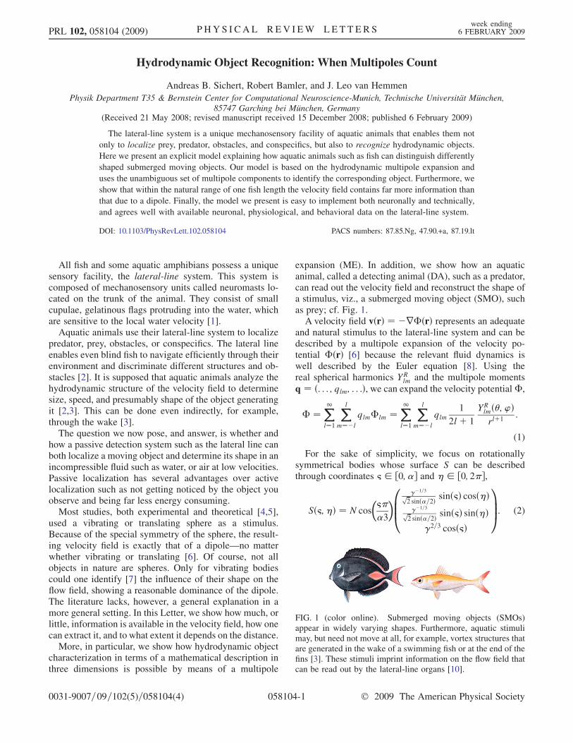
FIG. 2. Different shape parameters result in distinguishablesets of multipole components even for l � k ¼ 3 in (3); �increases along the vertical axis and � along the horizontalone. We have calculated q through a raster of 30 000 randomlydistributed positions on each moving object’s surface and usedobjects with length of about 5 cm and a matching moving speedv1 ¼ 0:01 m=s. Each volume is normalized to the volume of theunit sphere. It is therefore fair to say that the dipole stays almostconstant while q20 varies according to � and q30 to �. Therelative error 4ðkÞ :¼ jT q� wj=jwj on S as calculated forrotationally invariant elliptic bodies gives 4ðkÞ< 0:4 for k ¼3 and � < 2. It converges slowly to about 0.15 for k ! 1. For� � 2 a multipole expansion cannot describe the correct veloc-ity field. This, however, is not too restrictive. For example, thefish in Fig. 1 can be described by � � 1 (left fish) and � � 2(right fish).

PRL 102, 058104 (2009) P HY S I CA L R EV I EW LE T T E R Sweek ending

6 FEBRUARY 2009

058104-2

We note that the matrix T ðr0; riÞ depends on the SMOposition r0 and the position ri of the lateral-line organ i(DA). Noise is modeled by adding independent Gaussianrandom variables ni with mean 0 and standard deviation�n

to the wi. All positions r0 are of equal probability. Wetherefore take a Gaussian probability distributionpðq; r0Þ � expð�q2=2�2

qÞ. Instead of maximizing the

combined probability based on Bayes law, we maximizeits logarithm Lðq; r0Þ :¼ ln½pðq; r0jwÞ�. Defining � :¼�n=�q, we just have to maximize

Lðq; r0Þ ¼ �f½w�T ðr0; riÞq�2 þ �2q2g (6)

with respect to the multipole-moment vector q and r0. Thenecessary condition for a maximum of the likelihoodLðq; r0Þ at the correctly estimated position r0 is

@L

@qðq; r0Þjq¼q ¼ ½ðT TT þ �2Þq�T Tw�jq¼q ¼ 0; (7)

which leads to a linear system of equations solvable bymeans of the pseudoinverse technique [9],

q ¼ ðT TT þ �2Þ�1T Tw: (8)

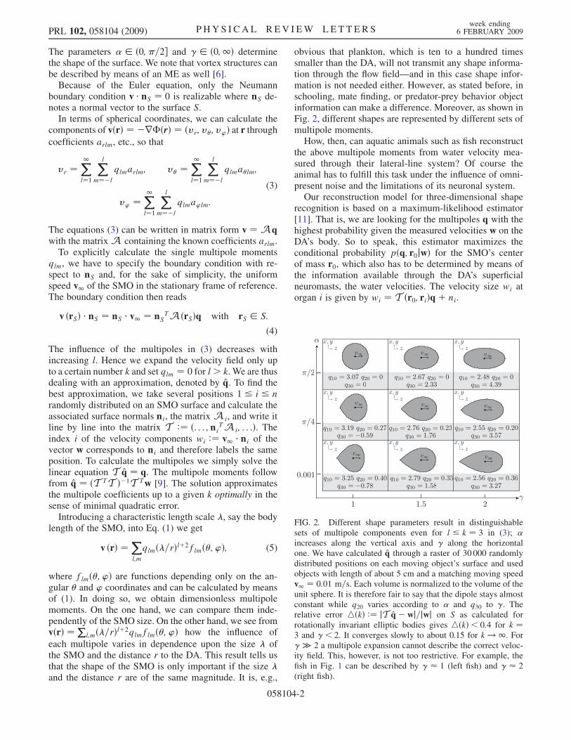
We estimate the set of multipoles q given only the mea-sured velocities w at the lateral-line organs. A neuronalimplementation of these calculations is straightforwardand can be done easily by neuronal hardware; see Fig. 3.Thus the position and the appropriate multipole momentscan be calculated neuronally.

To test whether it is possible for aquatic animals usingthe above method to determine SMO’s position and shape,we have applied noise to the input signal wi. We have used�n ¼ 10�4 m=s as standard deviation of the noise, whichcorresponds to the velocity threshold of Xenopus’s lateral-line organ [1]. Furthermore, we define a signal-to-noiseratio, SNR :¼ v1=�n, that dominates the performance ascompared to the number of neuromasts, cf. [12]. The more

multipoles we use, the more positions are of high proba-bility because one has more parameters to fit the measuredwi’s. Thus the estimated position gets ambiguous but theshape estimate improves. Choosing the right� for a certaink can compensate this effect and enables a faithful local-ization. In Fig. 4 we show the ability of our method toestimate the SMO position r0.Following the ansatz of the neuronal model (Fig. 3) we

have calculated the multipole moments at the estimatedposition, i.e., not only at the correct position but also atr0 þ �r where �r accounts for the continuity of real space,a limited number of map neurons as well as a slightlocalization uncertainty (Fig. 4). Our model can recon-struct qr0 even under noisy conditions and at slightlywrong positions [Fig. 5(a) and 5(b)]; for example, thefish bodies of Fig. 1 (see also Fig. 2) can be recognizedand distinguished. Thus object localization as well asobject recognition based on the estimation of multipolesis possible.In the following, we discuss the limitations of the pro-

posed method and likewise the theoretical limitation ofaquatic animals’ ability of object recognition. To comparethe quality of different multipole estimates q at different

distances d, we define �q :¼ffiffiffiffiffiffiffiffiffiffiffiffiffiffiffiffiffiffiffiffiffiffiffiffiffiffiffiffiffiffiffiffiffihðqlm � hqlmiÞ2i

p=hqlmi as a

quality measure. Here �q labels the normalized standard

deviation due to wrongly estimated positions rþ �r andnoise. For small �q the estimation error in qlm is small and,

in spite of a slightly wrong position, the shape parameter �can be recognized. For values �q > 1 a shape reconstruc-

tion based on the estimated qlm is impossible.For the octupole q30, the critical distance where the error

�q starts to grow extremely fast is SMO’s size itself. For

localization, the critical distance can be taken as the lengthof DA’s lateral-line system, say a fish length, which is in

FIG. 3. Neuronal implementation of (8) is straightforward. In afirst step ðAÞ ! ðBÞ the multipole components qlmðr0Þ (B) arecalculated for different positions r0 from the measured watervelocities wi at the neuromasts (A). This corresponds to a net-work of synaptic connections between the lateral line and thecentral nervous system. The strength of the individual connec-tions can be computed from the entries of the right-hand side of(8) or can be learned neuronally [14]. In a second step ðBÞ !ðCÞ, Lðq; r0Þ is calculated from the qr0, which can also be doneby feedforward connections, cf. (6). The maximum Lðq; r0Þindicates the correct position of the SMO and selects the optimalqr0 from step ðCÞ ! ðBÞ, cf. (7).

-10 -5 0 5 10-202468

10

-10 -5 0 5 10-202468

10

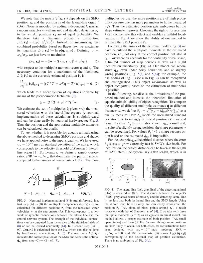
FIG. 4. The lateral line [(A), gray line] of the detecting animal(DA) is centered at ð0; 0Þ. The distance between the object’s(SMO, gray area) center of mass r0 and the detecting lateral lineis just less than both the lateral line and the SMO length. Usingthe dipole term ðk ¼ 1Þ only, we can easily reconstruct theposition r0 [(A), cloud of black points around r0], a resultconsistent with that of Franosch et al. [4]. If we take only threemultipole moments (k ¼ 3) as an efficient minimal model, ourmethod allows a proper estimate of both position [(A), smallopen circles] and form (cf. Fig. 5), even though more positionsare now likely to occur. For both cases, 40 reconstructions havebeen depicted with �n ¼ 10�4 m=s, moderate SNR :¼v1=�n ¼ 100, and 500 neuromasts. (B) shows log½Lðq; r0Þ�corresponding to the neuronal map of position estimation.There is no ambiguity; cf. Fig. 3(c).

PRL 102, 058104 (2009) P HY S I CA L R EV I EW LE T T E R Sweek ending

6 FEBRUARY 2009

058104-3

case of a predator hunting for prey larger than the criticallength of shape reconstruction (Fig. 6).

The ME method can quantify stimulus characteristics.Because the flow field need not be generated by a sub-

merged moving object alone, the method can also beapplied to characterize composite situations such asschooling or vortex structures found in the wake of afish. The ME is useful only if the distance between theobject (SMO) and detector (DA) is approximately of thesame size as the SMO, or shorter. Otherwise the MEreduces to its dipole simplification.Our object-recognition model agrees well with biologi-

cal findings and provides a theoretical understanding ofhydrodynamic object perception through the lateral line.Furthermore, we now understand the fundamental restric-tions for any (neuronal) evaluation of lateral-line data.Finally, these findings can also be applied to biomimetics[13], e.g., to improve passive naval navigation systems.A. B. S. and R. B. were supported by BCCN-Munich.

[1] H. Bleckmann, Reception of Hydrodynamic Stimuli inAquatic and Semiaquatic Animals (Fischer, New York,1994).

[2] C. von Campenhausen, I. Riess, and R. Weissert, J. Comp.Physiol. A 143, 369 (1981).

[3] S. Coombs, R. Anderson, C. B. Braun, and M.Grosenbaugh, J. Acoust. Soc. Am. 122, 1227 (2007).

[4] J.-M. P. Franosch, A. B. Sichert, M.D. Suttner, and J. L.van Hemmen, Biol. Cybern. 93, 231 (2005).

[5] S. Coombs and R.A. Conley, J. Comp. Physiol. A 180,401 (1997); B. Curcic-Blake and S.M. van Netten, J. Exp.Biol. 209, 1548 (2006).

[6] H. Lamb, Hydrodynamics (Cambridge University Press,Cambridge, England, 1932), 6th ed.; M. S. Howe, Theoryof Vortex Sound (Cambridge University Press, Cambridge,England, 2003).

[7] A. J. Kalmijn, in Sensory Biology of Aquatic Animals,edited by J. Atema, R. R. Fay, A. N. Popper, and W.N.Tavolga (Springer, New York, 1988), p. 83; G. G. Harris,in Marine Bioacoustics, edited by W.N. Tavolga(Pergamon Press, Oxford, 1964), p. 233.

[8] J. Goulet et al., J. Comp. Physiol. A 194, 1 (2008). For theinfluence of canal neuromasts, one can consult this papertoo.

[9] W.H. Press, S. A. Teukolsky, W. T. Vetterling, and B. P.Flanery, Numerical Recipes in C (Cambridge UniversityPress, Cambridge, England, 1995), 2nd ed., p. 34, thepseudoinverse.

[10] From NOAA’s Historic Fisheries Collection; IDs: fish3078and fish3039.

[11] B. L. van der Waerden, Mathematical Statistics (Springer,New York, 1969); M. Jazayeri and J. A. Movshon, Nat.Neurosci. 9, 690 (2006).

[12] See EPAPS Document No. E-PRLTAO-102-005908 fordetails on the model performance and a full set of esti-mated multipoles. For more information on EPAPS, seehttp://www.aip.org/pubservs/epaps.html.

[13] Y. Yang et al., Proc. Natl. Acad. Sci. U.S.A. 103, 50(2006).

[14] J.-M. P. Franosch, M. Lingenheil, and J. L. van Hemmen,Phys. Rev. Lett. 95, 078106 (2005).

5 10 15 2000.20.40.60.81.01.21.4

02468

101214

FIG. 6. Relative reconstruction error �q30 (dashed line) of themultipole component q30 as defined in the main text. It showsthat for distances d larger than a moving object’s size (5 cm)multipole reconstruction is not possible. The solid line depictsthe localization error hkr0 � r0ki, which starts to grow fast at adistance comparable to the length of the detecting animal(10 cm). This agrees well with experimental findings wherelocalization performance starts decreasing at distances beyondthe fish body size [5]. For discrimination tasks, fish have to bevery close to the object under investigation [2].

1.0 1.2 1.4 1.6 1.8 2.0-0.5

0

1.0

1.5

1.0 1.2 1.4 1.6 1.8 2.0-0.5

0

1.0

1.5

1.0 1.2 1.4 1.6 1.8 2.0-0.5

0

1.0

1.5

1.0 1.2 1.4 1.6 1.8 2.0-0.5

0

1.0

1.5

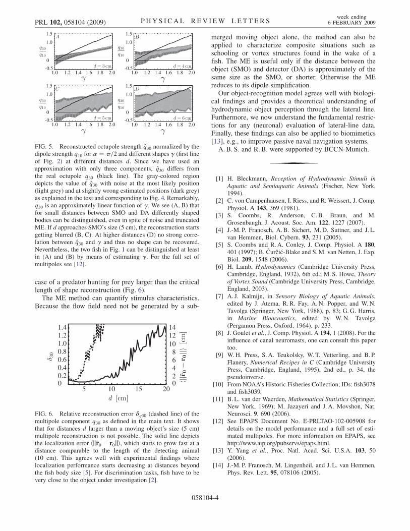
FIG. 5. Reconstructed octupole strength q30 normalized by thedipole strength q10 for � ¼ �=2 and different shapes � (first lineof Fig. 2) at different distances d. Since we have used anapproximation with only three components, q30 differs fromthe real octupole q30 (black line). The gray-colored regiondepicts the value of q30 with noise at the most likely position(light grey) and at slightly wrong estimated positions (dark grey)as explained in the text and corresponding to Fig. 4. Remarkably,q30 is an approximately linear function of �. We see (A, B) thatfor small distances between SMO and DA differently shapedbodies can be distinguished, even in spite of noise and truncatedME. If d approaches SMO’s size (5 cm), the reconstruction startsgetting blurred (B, C). At higher distances (D) no strong corre-lation between q30 and � and thus no shape can be recovered.Nevertheless, the two fish in Fig. 1 can be distinguished at leastin (A) and (B) by means of estimating �. For the full set ofmultipoles see [12].

PRL 102, 058104 (2009) P HY S I CA L R EV I EW LE T T E R Sweek ending

6 FEBRUARY 2009

058104-4