In press (4/25/04) – Seismological Research Letters 1

Hydroacoustic Constraints on the Rupture Duration, Length and Speed of the Great

Sumatra-Andaman Earthquake

Maya Tolstoy and DelWayne R. Bohnenstiehl

Lamont-Doherty Earth Observatory of Columbia University,

61 Route 9W, Palisades, NY 10964

INTRODUCTION

On December 26th 2004, one of the largest recorded earthquakes occurred, triggering

a devastating tsunami that killed an estimated 300,000 people. The event was initially

classified as Mw=9.0 based on the analysis of seismic body and surface waves (Harvard

CMT, 2004; Ji, 2005; Park et al., 2005). However, classical methods of magnitude

calculation are hampered by the long duration of the event, since late arriving phases

from the earliest portion of the rupture may obscure first-arriving energy sourced from

other portions of the rupture. This same phenomenon also limits our ability to constrain

the earthquake’s duration, length and speed of propagation.

To get around these limitations, Stein and Okal (2005) studied Earth’s low order

normal modes to estimate the size of the earthquake. Their results indicated a moment of

1.3 x 1030 dyn-cm (Mw=9.3), which is ~2.5 times larger than initial reports, and a

centroid position near 7°N. In contrast with previous analyses, which had suggested

displacement occurred primarily along the southern third of the aftershock region (Ji ,

2005; Yamanaka, 2005; Yagi, 2005), these results argue that significant slip occurred

along the entire aftershock zone.

2

For shallow submarine earthquakes, hydroacoustic recordings of Tertiary (T-) waves

can provide additional constraints on rupture length, as well as the velocity and direction

of rupture propagation (e.g., Bohnenstiehl et al., 2004). T-waves are formed when

seismically generated energy is scattered at the seafloor-ocean interface and becomes

trapped in the ocean’s low-velocity waveguide, which is known as the SOund Fixing And

Ranging (SOFAR) channel (Tolstoy and Ewing, 1950). Locating the source of a T-wave,

therefore, does not necessarily provide an estimate of the earthquake epicenter, but rather

the position of the T-wave radiator. This is particularly true for the subduction zone

environment (de Groot-Hedlin and Orcutt, 1999; Graeber and Piserchia, 2004), where

long land paths may exist prior to acoustic conversion. In such instances, the T-wave

radiator locations might vary with azimuth to a particular station, adding ambiguity to the

locations derived from multiple stations. Great care should be taken in evaluating the

influence of local bathymetric variations within the source region and considering

whether a T-wave radiator location is representative of the earthquake’s epicenter.

In part because of limitations relative to local three-component seismic data, T-waves

have not been widely exploited for earthquake studies, except in the case of mid-ocean

ridge investigations (e.g. Fox et al., 1995; Fox et al., 2001; Smith et al., 2002), where

local seismic data is very expensive to obtain. For remote portions of an ocean basin, a

small number of hydrophones can improve the magnitude of completeness of a mid-

ocean ridge earthquake catalog by more than one order of magnitude (Bohnenstiehl et al.,

2002). T-wave data tends to play a complimentary role to seismic data, and often can

yield tectonic and geological information that would not have been obtained using

existing seismic networks.

3

The Indian Ocean is the site of three hydroacoustic stations operated as part of the

International Monitoring System (IMS). These data are usually only available through

National Data Centers of Signatory Countries to the Comprehensive Test Ban Treaty.

Within the U.S., only organizations with active contracts to use the data, generally with

the Air Force, have access. Because of the unusual global importance of this event,

however, some data from the IMS have been made openly available for December 26th

2004 (http://www.rdss.info).

At each Indian Ocean hydroacoustic station, three hydrophones are deployed in a

triangular configuration with a ~2 km spacing between sensors. These hydrophone triads

are moored offshore of the Diego Garcia atoll, southwestern Australia and Crozet Island.

Our analysis is focused on signals recorded at the Diego Garcia South (DGS or H08S)

triad (Figure 1), since this station provides the best azimuthal coverage, with minimally

variable crustal paths, from the Sumatran-Andaman rupture zone. The frequency

response of the hydrophone system is flat to within 3 dB over the range of 3-100 Hz.

HYDROACOUSTIC ANALYSIS AND METHODS

To identify T-wave radiator locations, azimuthal estimates are derived by inverting

the differential travel times between sensors within the DGS hydrophone triad. Travel

time differences between each pair of hydrophones (ti,j) within the station’s triad were

derived from the cross-correlation of the 4-6 Hz bandpassed signal arrivals, within 10 s

windows having 50% overlap. These delay times were used in a plane wave fitting

inversion to determine the horizontal slowness components (px, py) and estimate the back-

azimuth to the source region (e.g., Del Pezzo and Giudicepietro, 2002). This relation

4

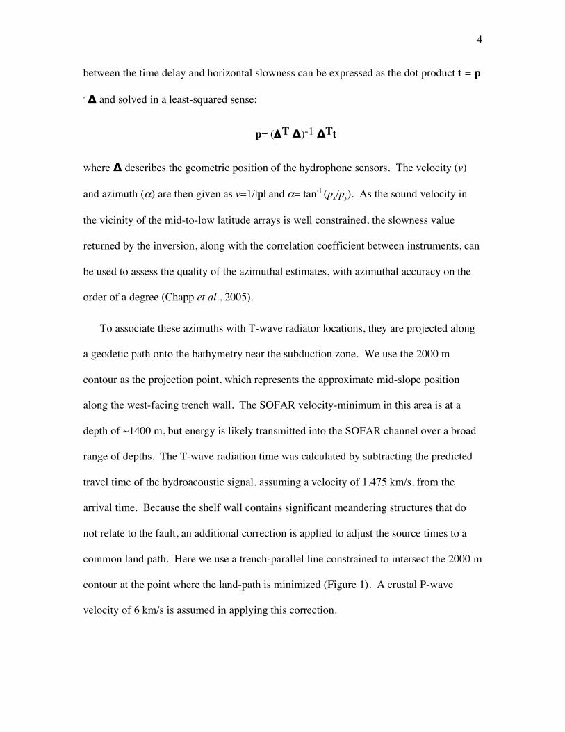
between the time delay and horizontal slowness can be expressed as the dot product t = p

. Δ and solved in a least-squared sense:

p= (ΔT Δ)-1 ΔTt

where Δ describes the geometric position of the hydrophone sensors. The velocity (v)

and azimuth (α) are then given as v=1/|p| and α= tan-1 (px/py). As the sound velocity in

the vicinity of the mid-to-low latitude arrays is well constrained, the slowness value

returned by the inversion, along with the correlation coefficient between instruments, can

be used to assess the quality of the azimuthal estimates, with azimuthal accuracy on the

order of a degree (Chapp et al., 2005).

To associate these azimuths with T-wave radiator locations, they are projected along

a geodetic path onto the bathymetry near the subduction zone. We use the 2000 m

contour as the projection point, which represents the approximate mid-slope position

along the west-facing trench wall. The SOFAR velocity-minimum in this area is at a

depth of ~1400 m, but energy is likely transmitted into the SOFAR channel over a broad

range of depths. The T-wave radiation time was calculated by subtracting the predicted

travel time of the hydroacoustic signal, assuming a velocity of 1.475 km/s, from the

arrival time. Because the shelf wall contains significant meandering structures that do

not relate to the fault, an additional correction is applied to adjust the source times to a

common land path. Here we use a trench-parallel line constrained to intersect the 2000 m

contour at the point where the land-path is minimized (Figure 1). A crustal P-wave

velocity of 6 km/s is assumed in applying this correction.

5

CONSTRAINTS ON RUPTURE DURATION, LENGTH AND SPEED

Figure 2 shows the T-wave signal generated by the Great Sumatran-Andaman

Earthquake, as recorded at the DGS station, along with its spectrogram and associated

azimuth to the T-wave radiator. The southernmost azimuth (t=1900) associated with the

initial large-amplitude arrival is within 0.4° of the epicenter location (3.3°N, 95.8° E),

which lies ~165 km to the ENE from the trench wall (Figure 1). The azimuthal data

show a northward trend (decreasing azimuth from DGS), as well as an initial small

southerly trend associated with a gradual rise to the high amplitude onset of the T-wave

(t=1865-1900). This initial trend of arrival azimuths to the south represents energy

sourced from the epicentral region, but traveling on a less direct path. While this

northerly path is longer, a greater proportion of it is spent traveling as a P-wave, because

of the NW trend of the shelf, resulting in earlier arrival at DGS. The low energy of the

arrivals, relative to the direct arrival is indicative of the less direct path (Graeber and

Piserchia, 2004).

For these earliest arriving signals, the T-wave radiation time is estimated by

subtracting the predicted acoustic travel time from the arrival time at DGS. Differencing

the radiation time with the event’s origin time provides an estimate of the crustal travel

time and apparent crustal velocity. As the epicenter azimuth is approached (t=1900 s),

apparent crustal velocity decreases, with the arrival most closely aligned with the

epicentral azimuth exhibiting an apparent velocity of 2.8 km/s. This is a reasonable

rupture velocity in this setting (Venkataraman and Kanamori, 2004) and consistent with

the initial propagation of the rupture up dip, as well as along strike. Near maximum

peak-amplitudes are reached as the rupture shallows (Figure 2), suggesting that the T-

6

wave signal may be dominated by seismic energy radiated from the shallowest portions

of the rupture zone.

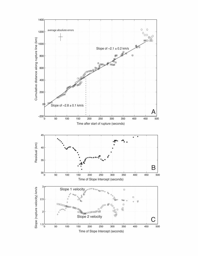
Figure 3A shows the cumulative distance along the rupture front, as estimated from

the T-wave radiator positions (corrected for differential land paths), versus the source

time. The slope of these points provides an estimate of the lateral rupture speed during

the earthquake. A least-squares fit to the entire dataset yields a mean velocity of 2.4 ±

0.2 km/s, consistent with the 2.5 km/s obtained by Ni et al. (2005) from the directivity of

radiated high-frequency (2-4 Hz) seismic energy. The initial ~180 s of the rupture,

however, is fit better by a velocity of ~2.8±0.1 km/s, with the last ~300 s of the rupture

characterized by a velocity of ~2.1± 0.2 km/s. This suggests a 'two-phase' rupture

process.

To investigate the timing of this transition in rupture speed, the goodness-of-fit was

evaluated for a series of best-fitting ‘two-slope’ models with the break points ranging

from ~50-450 s (Figure 3B). The misfit between the predicted and observed position of

the rupture front (T-wave radiator location) is minimized for break points between 150-

190 s, with a broader minimum between 150-290 s (Figure 3B). Across this range, least-

squares velocity estimates are consistently higher for the first portion of the rupture

(slope 1), relative to the second (slope 2), with the propagation speed slowing during

roughly the second third of the rupture (Figure 3C).

Also constrained in Figure 3 are the duration of the rupture, which is ~480 s, and the

total rupture length, which is ~1200 km, similar to recent interpretations based on

aftershock distribution (Stein and Okal, 2005) and high-frequency energy radiation (Ni et

al., 2005). This length and duration indicates the initial interpreted rupture length of only

7

400 km over 200 s, led to underestimation of the magnitude (Stein and Okal, 2005). The

rupture length of 1200 km makes it one of the longest ruptures ever recorded, ripping all

the way from its epicenter near 3.3° N, 95.8° E to the end of the subduction zone at a

latitude of ~13.5°N.

While the mainshock moment tensor solution indicates thrust faulting, aftershocks

show an increasing strike-slip component further north along the fault (Kim, 2005,

Harvard CMT, 2004-2005). This is consistent with an increasingly oblique relative

motion between the Indian and Burma plates (Bird, 2003). The rupture terminates at the

latitude of the pole of rotation (to within the error of the azimuth estimate) between these

two plates, suggesting that the northern boundary of the subduction zone represents a

tectonic barrier to rupture propagation—limiting the length and moment of this great

earthquake.

Previous studies have suggested that many tsunamigenic subduction zone earthquakes

contain a slow rupture component, which is manifested by a low radiation efficiency

(Okal et al. , 2003; Venkataraman and Kanamori, 2004) and slow rupture velocity

(Venkataraman and Kanamori, 2004). Such behavior has been linked to the propagation

through low-rigidity sediments within the accretion prism (Fukao, 1979) or the

heterogeneities along the subduction interface that lead to greater energy dissipation

during rupture (Tanioka et al., 1997; Polet and Kanamori, 2000). The later portion of the

Great Sumatra-Andaman earthquake is characterized by an average rupture velocity of

2.1 ± 0.2 km/s. This approaches the 1-2.0 km/s range cited for three tsunamogenic

earthquakes in the global compilation of Venkataraman and Kanamori (2004).

8

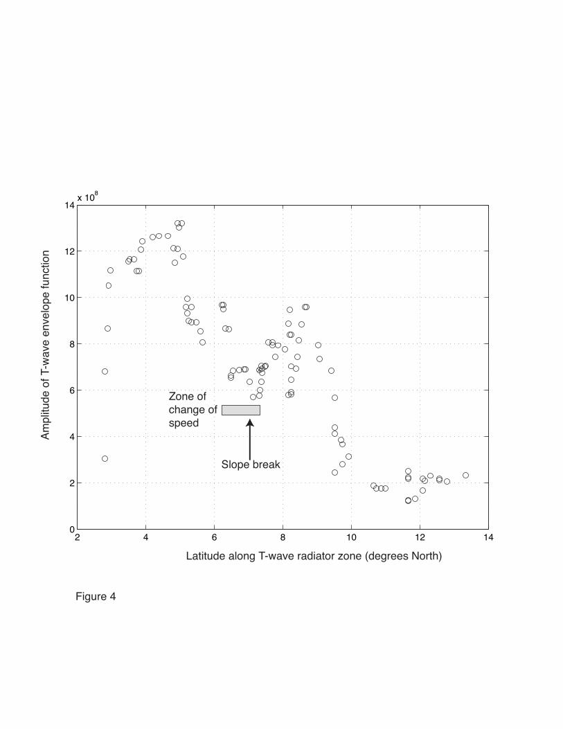
Our observations indicate that high-frequency T-wave energy was radiated along the

length of the rupture zone. The transition in rupture velocity occurs at a local minimum in

the T-wave amplitude (Figure 4), which coincides spatially with a change in the trend of

the aftershocks near 7° N (Stien and Okal, 2005). The occurrence of local amplitude

maxima sourced from ~4-5°N and ~8-9°N are consistent with recent high-frequency

radiation calculations (Ishii et al., 2005) that indicate two peaks in energy released at ~80

s and ~320 s after onset. The later portion of the T-wave packet (sourced from north of

~9.5° N latitude) exhibits amplitudes that are roughly a factor of four lower than the

earliest portion of the rupture (Figure 4). This may be consistent with lower radiation

efficiency during the slower phase of rupture. However, variability in the efficiency of

T-wave coupling into the SOFAR channel, associated with changes in orientation of the

trench wall, also may contribute to this pattern.

IMPLICATIONS FOR EMERGENCY RESPONSE

When hydroacoustic data are available in near real-time, they may be used for

rapid assessment of the spatial extent and moment of large submarine earthquakes. Such

information could provide additional warning time for mobilizing rescue and relief

efforts. It has long been postulated that T-waves might be useful in predicting tsunamis

(Ewing et al., 1950), and recent work proposes a quantitative method for doing so (Okal

et al., 2003). Our results show that reliable early estimates of event size might be made

by simply studying T-wave duration (Okal and Talandier, 1986) and projecting azimuthal

information onto the bathymetry within the source region. This could be accomplished

9

using a sparse network of small aperture arrays, similar to those deployed as part of the

IMS.

SUMMARY

T-wave azimuths and arrival times measured by a hydrophone triad off the island

of Diego Garcia for the December 26th 2004 Great Sumatra-Andaman earthquake indicate

a rupture duration of ~8 minutes and length of ~1200 km. Rupture speed slows from

2.8± 0.1 to 2.1 ± 0.2 km/s after propagating ~450 km northward from the epicenter

(3.3°N, 95.8°E). The latest arriving acoustic energy is sourced from the northern

boundary of the Indian-Burma subduction zone at ~13.5°N latitude. Real-time analysis

of hydroacoustic data may provide an effective method for rapidly evaluating the size and

location of a large submarine earthquake.

ACKNOWLEDGEMENTS

We acknowledge the SMDC for access to the data, and would like to thank P. Richards

and W.-Y. Kim for useful discussions. We also thank Susan Hough for suggestions that

significantly improved the paper.

REFERENCES

Bird, P., (2003). An updated digital model of plate boundaries, Geochemistry.

Geophysics Geosystems 4, doi:10.1029/2001GC000252.

10

Bohnenstiehl, D.R., M. Tolstoy, D.K. Smith, C.G. Fox, and R. Dziak, (2002). The decay

rate of aftershock sequences in the mid-ocean ridge environment: An analysis

using hydroacoustic data, Tectonophysics 354:49-70.

Bohnenstiehl, D.R., M. Tolstoy, and E. Chapp, (2004). Breaking into the plate: A 7.6 Mw

fracture-zone earthquake adjacent to the Central Indian Ridge, Geophysical

Research Letters 31, L02615.

Chapp, E., D.R. Bohnenstiehl, and M. Tolstoy, (2005). Sound-Channel Observations of

Ice-Generated Tremor in the Indian Ocean, Geochemistry Geophysics Geosystems

in press.

de Groot-Hedlin, C. D. and J.A. Orcutt, (1999). Synthesis of earthquake-generated T-

waves, Geophysical Research Letters 26, 1227–1230.

Del Pezzo, E. and F. Giudicepietro, (2002). Plane wave fitting method for a plane, small

aperture, short period seismic array: a MATHCAD program, Computational

Geoscience 28, 59-64.

Ewing, M., I. Tolstoy, and F. Press, (1950). Proposed use of the T-phase in tsunami

warning systems, Bulletin of the Seismological Society of America 40, 53–58.

Fox, C.G., W.E. Radford, R.P. Dziak, T.-K. Lau, H. Matsumoto, and A.E. Schreiner,

(1995). Acoustic detection of a seafloor spreading episode on the Juan de Fuca

Ridge using military hydrophone arrays, Geophysical Research Letters 22, 131-

134.

11

Fox, C.G., H. Matsumoto, and T.K.A. Lau, (2001). Monitoring Pacific Ocean seismicity

from an autonomous hydrophone array, Journal of Geophysical Research 106,

4183-4206.

Fukao, Y., (1979). Tsunami earthquake and subduction processes near deep sea trenches,

Journal of Geophysical Research 84, 2303-2314.

Graeber, F. M. and P.F. Piserchia, (2004). Zones of T-wave excitation in the NE Indian

Ocean mapped using variations in back azimuth over time obtained from multi-

channel correlation of IMS hydrophone triplet data, Geophysical Journal

International 158, doi: 10.1111/j.1365-246X.2004.02301.x.

Harvard CMT, (2004).

http://neic.usgs.gov/neis/eq_depot/2004/eq_041226/neic_slav_hrv.html

Harvard CMT, (2004-2005). http://www.seismology.harvard.edu

Ishii, M., P. Shearer, H. Houston, and J.Vidale, (2005).

http://mahi.ucsd.edu/shearer/SUMATRA/ishii.html

Ji, C., (2005). http://neic.usgs.gov/neis/eq_depot/2004/eq_041226/neic_slav_ff.html

Kim, W.-Y., (2005). http://www.iris.iris.edu/sumatra/

Ni, S., H. Kanamori, and D. Helmberger, (2005). Energy radiation from the Sumatra

earthquake, Nature 484, 582.

Okal, E.A., P.-J. Alasset, O. Hyvernaud, and F. Schindelé, (2003). The deficient T waves

of tsunami earthquakes, (2003). Geophysical Journal International 152, 416-432.

12

Okal, E.A. and J. Talandier, (1986). T-wave duration, magnitudes and seismic moment of

an earthquake—application of tsunami warning, Journal of Physics of the Earth

34, 19-42.

Park, J., K. Anderson, R. Aster, R. Butler, T. Lay, and D. Simpson, (2005). Global

seismographic network records the great Sumatra-Andaman Earthquake EOS

Transactions of the American Geophysical Union 86, 57-64.

Polet, J. and H. Kanamori, (2000). Shallow subduction zone earthquakes and their

tsunamigenic potential, Geophysical Journal International 142, 684-702.

Smith, D.K., M. Tolstoy, C.G. Fox, D.R. Bohnenstiehl, H. Matsumoto, M. J. Fowler,

(2002). Hydroacoustic Monitoring of Seismicity at the Slow Spreading Mid-

Atlantic Ridge, Geophysical Research Letters 10.1029/2001GL013912,.

Stein, S. and E.A. Okal, (2005). Sumatra earthquake: Gigantic and slow, Nature 484,

581-582.

Tanioka, Y., L.J. Ruff, and K. Satake, (1997). What controls the lateral variation of large

earthquake occurrence along the Japan trench?, Island Arc 6, 261-266.

Tolstoy, I. and W.M. Ewing, (1950). The T phase of shallow-focus earthquakes, Bulletin

of the Seismological Society of America 40, 25-51.

Yagi, Y., (2005). http://iisee.kenken.go.jp/staff/yagi/eq/Sumatra2004/Sumatra2004.html

Yamanaka, Y., (2005). http://www.eri.utokyo.ac.jp/sanchu/Seismo_Note/

13

Venkataraman, A. and H. Kanamori, (2004). Observational constraints on the fracture

energy of subduction zone earthquakes, Journal of Geophysical Research 109,

doi:10.1029/2003JB0025249.

FIGURE CAPTIONS

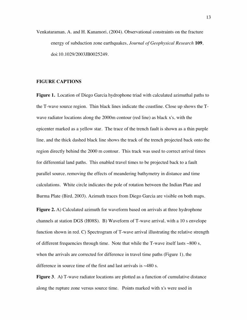
Figure 1. Location of Diego Garcia hydrophone triad with calculated azimuthal paths to

the T-wave source region. Thin black lines indicate the coastline. Close up shows the T-

wave radiator locations along the 2000m contour (red line) as black x's, with the

epicenter marked as a yellow star. The trace of the trench fault is shown as a thin purple

line, and the thick dashed black line shows the track of the trench projected back onto the

region directly behind the 2000 m contour. This track was used to correct arrival times

for differential land paths. This enabled travel times to be projected back to a fault

parallel source, removing the effects of meandering bathymetry in distance and time

calculations. White circle indicates the pole of rotation between the Indian Plate and

Burma Plate (Bird, 2003). Azimuth traces from Diego Garcia are visible on both maps.

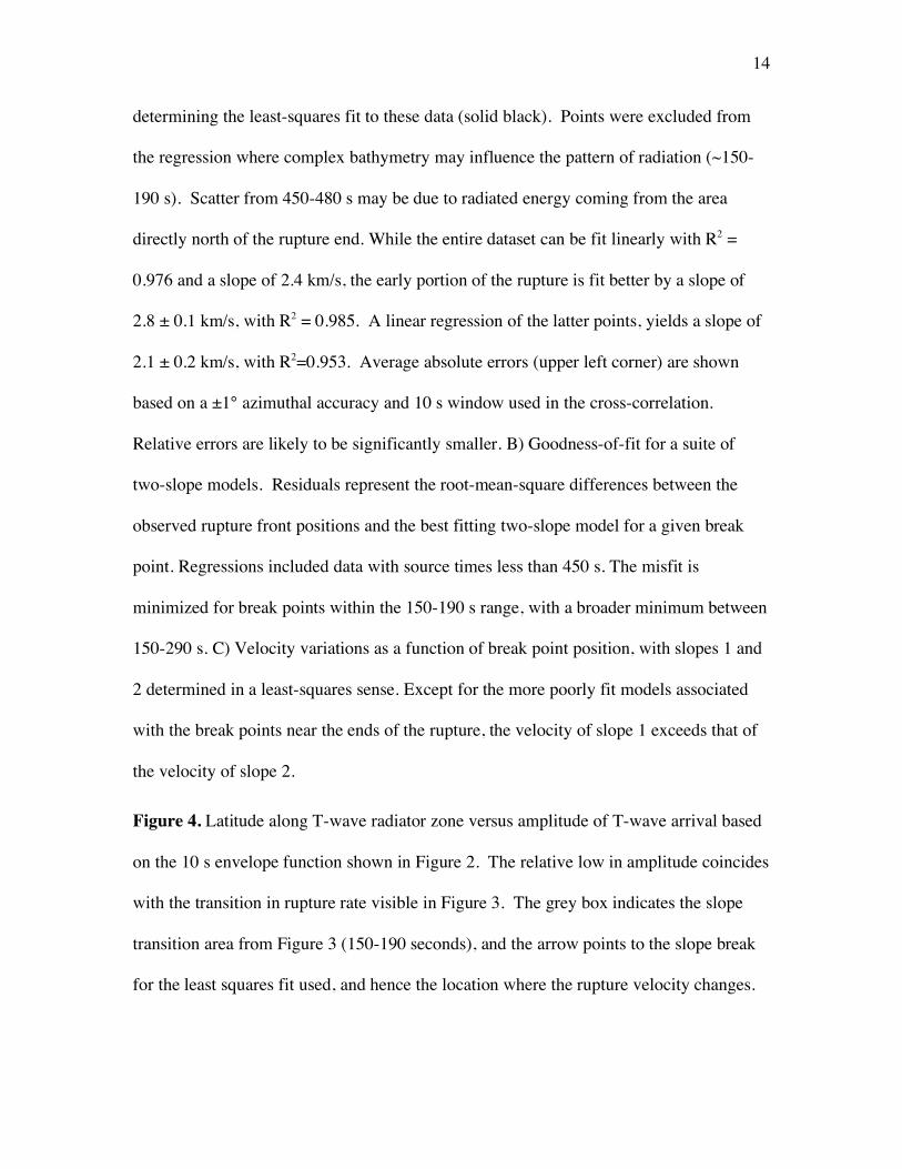
Figure 2. A) Calculated azimuth for waveform based on arrivals at three hydrophone

channels at station DGS (H08S). B) Waveform of T-wave arrival, with a 10 s envelope

function shown in red. C) Spectrogram of T-wave arrival illustrating the relative strength

of different frequencies through time. Note that while the T-wave itself lasts ~800 s,

when the arrivals are corrected for difference in travel time paths (Figure 1), the

difference in source time of the first and last arrivals is ~480 s.

Figure 3. A) T-wave radiator locations are plotted as a function of cumulative distance

along the rupture zone versus source time. Points marked with x's were used in

14

determining the least-squares fit to these data (solid black). Points were excluded from

the regression where complex bathymetry may influence the pattern of radiation (~150-

190 s). Scatter from 450-480 s may be due to radiated energy coming from the area

directly north of the rupture end. While the entire dataset can be fit linearly with R2 =

0.976 and a slope of 2.4 km/s, the early portion of the rupture is fit better by a slope of

2.8 ± 0.1 km/s, with R2 = 0.985. A linear regression of the latter points, yields a slope of

2.1 ± 0.2 km/s, with R2=0.953. Average absolute errors (upper left corner) are shown

based on a ±1° azimuthal accuracy and 10 s window used in the cross-correlation.

Relative errors are likely to be significantly smaller. B) Goodness-of-fit for a suite of

two-slope models. Residuals represent the root-mean-square differences between the

observed rupture front positions and the best fitting two-slope model for a given break

point. Regressions included data with source times less than 450 s. The misfit is

minimized for break points within the 150-190 s range, with a broader minimum between

150-290 s. C) Velocity variations as a function of break point position, with slopes 1 and

2 determined in a least-squares sense. Except for the more poorly fit models associated

with the break points near the ends of the rupture, the velocity of slope 1 exceeds that of

the velocity of slope 2.

Figure 4. Latitude along T-wave radiator zone versus amplitude of T-wave arrival based

on the 10 s envelope function shown in Figure 2. The relative low in amplitude coincides

with the transition in rupture rate visible in Figure 3. The grey box indicates the slope

transition area from Figure 3 (150-190 seconds), and the arrow points to the slope break

for the least squares fit used, and hence the location where the rupture velocity changes.

Figure 1

-7000 -6000 -5000 -4000 -3000 -2000 -1000 0 1000 2000 3000

Elevation (m)

60°E 70°E 80°E 90°E 100°E 90°E 92°E 94°E 96°E

20°N

10°S

0°

10°N

14°N

12°N

10°N

8°

6°

4°

2°

DGS

1600 1800 2000 2200 2400 2600 2800 300040

50

60

70

Time after Event Origin Time (seconds)

Azim

uth

from

DG

S (d

eg)

1800 2000 2200 2400 2600 2800

−1

−0.5

0

0.5

1

x 109

Time after Event Origin Time (seconds)

Ampl

itude

Time after 1600 seconds after Event Origin Time (seconds)

Freq

uenc

y

0 200 400 600 800 1000 12000

50

100

Figure 2

Initialramp-up

1600 1800 2000 2200 2400 2600 2800 3000

Time after Event Origin Time (seconds)

A

B

C

0 50 100 150 200 250 300 350 400 450 50030

35

40

45

0 50 100 150 200 250 300 350 400 450 5001.5

2

2.5

3

0 50 100 150 200 250 300 350 400 450 500−200

0

200

400

600

800

1000

1200

1400

Slope of ~2.1 ± 0.2 km/s

Slope of ~2.8 ± 0.1 km/s

Cum

ulat

ive

dist

ance

alo

ng ru

ptur

e lin

e (k

m)

Time after start of rupture (seconds)

average absolute errors

Res

idua

l (km

)S

lope

(rup

ture

vel

ocity

) km

/s

Time of Slope Intercept (seconds)

Time of Slope Intercept (seconds)

A

B

C

Slope 1 velocity

Slope 2 velocity

2 4 6 8 10 12 140

2

4

6

8

10

12

14x 108

Figure 4

Latitude along T-wave radiator zone (degrees North)

Ampl

itude

of T

-wav

e en

velo

pe fu

nctio

n

Slope break

Zone of change ofspeed