Journal of Hydraulic Research Vol. 42, No. 1 (2004), pp. 43–54

© 2004 International Association of Hydraulic Engineering and Research

Hydraulics of stepped chutes: The transition flow

L’hydraulique des chutes en marches d’escalier: L’écoulement de transitionH. CHANSON,Reader, Fluid Mechanics, Hydraulics and Environmental Engineering, The University of Queensland, Brisbane QLD4072, Australia. Email: h.chanson@uq.edu.au

LUKE TOOMBES,Associate Lecturer, Fluid Mechanics, Department of Civil Engineering, The University of Queensland,Brisbane QLD 4072, Australia

ABSTRACTStepped spillway flows may behave as a succession of free-falling nappes at low flows and as a skimming flow at large discharges. However there isa range of intermediate flow rates characterised by a chaotic flow motion associated with intense splashing: i.e. the transition flow regime. Detailedair–water flow properties in transition flows were measured in two large experimental facilities. The results provide a complete characterisation oftheair concentration, velocity and bubble count rate distributions. They highlight some difference between the upper and lower ranges of transition flowsin terms of longitudinal free-surface profiles and air concentration distributions. Overall a dominant feature is the very-strong free-surface aeration,well in excess of observed data in smooth-invert and skimming flows.

RÉSUMÉLes écoulements sur les déversoirs en marches d’escalier peuvent se comporter comme une succession des nappes en chute libres aux faibles débitset comme un écoulement écumant aux grands débits. De sorte qu’il y a toute une gamme de débits intermédiaires caractérisés par un mouvementchaotique d’écoulement lié à un éclaboussement intense: i.e. le régime d’écoulement de transition. Des propriétés détaillées de l’écoulement dumélange air-eau dans des écoulements de transition ont été mesurées dans deux grands équipements expérimentaux. Les résultats fournissent unecaractérisation complète de la concentration d’air, des distributions de vitesse et du taux de bulles. Ils mettent en lumière une certaine différence entreles gammes supérieures et inférieures des écoulements de transition en termes de profils de surface libre et distributions longitudinales de concentrationen air. De façon générale un caractère dominant est l’aération très forte de surface libre, bien au-dessus des données observées dans les écoulementslisses inversés et écumants.

Keywords: Stepped spillway; transition flow regime; free-surface aeration; chaotic flow pattern; experimental study.

Introduction

In a stepped chute, low flows behave as a succession of free-falling nappes: i.e. the nappe flow or jet flow regime (e.g. Horner,1969). For a given step and chute geometry, large flows skimover the pseudo-invert formed by the step edges: i.e. the skim-ming flow regime. The cavity formed by the steps is filled andstrong cavity recirculation is observed beneath the main stream(e.g. Rajaratnam, 1990). The conditions for the transition fromnappe to skimming flows were discussed by Chanson (1996) andChamani and Rajaratnam (1999) who used the term “onset ofskimming flow”. Few researchers discussed specifically the tran-sitory flow conditions between nappe and skimming flow: e.g.Elviro and Mateos (1995). Ohtsu and Yasuda (1997) were thefirst to define the concept of a “transition flow” regime althoughthey did not elaborate on its flow properties. Up to date littleinformation is available on transition flows.

It is the purpose of this study to provide a comprehensivestudy of transition flows down stepped chutes. Air–water flow

Revision received June 12, 2003. Open for discussion till June 30, 2004.

43

measurements were conducted in two large facilities with slopesranging from 3.4 to 22◦ and equipped with large step heights.A detailed characterisation of the air–water flow properties isprovided.

Experimental configuration

New experiments were conducted at the University of Queens-land in two large-size facilities (Table 1). One facility was a24-m long 0.5-m wide channel made of planed wooden boards.Two stepped inverts were used. The flume 1 consisted of ten0.143-m high, 2.4-m long horizontal steps while flume 2 hadeighteen 0.071-m high, 1.2-m long flat steps. For all experi-ments, the first drop was located 2.4 m downstream of a smoothnozzle, and the channel invert upstream of the vertical dropwas flat and horizontal. Water was supplied by a pump, witha variable-speed electronic controller (TaianTM T-verter K1-420-M3 adjustable frequency AC motor drive), enabling an accurate

44 H. Chanson and Luke Toombes

Table 1 Summary of experimental flow configurations.

Ref. α h qw Observed flow regime Remarksdeg. m m2/s

(1) (2) (3) (4) (5) (6)

Flume 1 3.4 0.143 0.08–0.140 Nappe & Transition flows L= 24 m. W = 0.5 m. Supercritical inflow: do = 0.03 m. Flathorizontal steps. Experiments CR98.

Flume 1 3.4 0.071 0.08–0.130 Nappe, Transition & Skimming flows L= 24 m. W = 0.5 m. Supercritical inflow: do = 0.03 m. Flathorizontal steps. Experiments EV200a.

Flume 3 21.8 0.10 0.04–0.18 Nappe, Transition & Skimming flows L= 3.0 m. W = 1 m. Broad-crest with smooth inflow side-wall convergent (4.8 : 1 contraction). Low upstream turbulence. Flathorizontal steps. Experiments EV200b & TC200.

Flume 4 15.9 0.10 0.05–0.26 Nappe, Transition & Skimming flows L= 4.2 m. W = 1 m. Broad-crest with smooth inflow side-wall convergent (4.8 : 1 contraction). Low upstream turbulence. Flathorizontal steps. Experiments TC201.

Notes: h= step height; L= chute length; W= chute width.

discharge adjustment in a closed-circuit system. The flow rateswere measured with a DallTM tube flowmeter, calibrated on site.The accuracy on the discharge measurement was about 2%.

Another channel was 5-m long, 1-m wide. Waters were sup-plied from a large feeding basin leading to a sidewall convergent.Two slopes were tested. One geometry consisted of a 0.88-m longbroad-crested weir with upstream rounded corner followed bynine identical steps (h= 0.1 m, l = 0.35 m) made of marine ply.The second geometry consisted of a 0.6-m long broad-crestedweir followed by nine steps (h= 0.1 m, l = 0.25 m). Thestepped chute was 1-m wide with perspex sidewalls, followed bya horizontal concrete-invert canal ending in a dissipation pit. Theflow rate was delivered by a pump controlled with an adjustablefrequencyAC motor drive, enabling an accurate discharge adjust-ment in a closed-circuit system. The discharge was measuredfrom the upstream head above crest with an accuracy of about2% (Bos, 1976). Figure 1 illustrates the chute geometry.

Further details on the experimental facilities may be found inChanson and Toombes (1998, 2001).

Instrumentation and measurement techniques

Clear-water flow depths and velocities were measured with apoint gauge and a Prandtl–Pitot tube(� = 3.3 mm) respec-tively. Air–water flow properties were measured using single-tipand double-tip conductivity probes. For the double-tip probe,the probe sensors(� = 0.025 mm, 7.775 mm spacing betweensensors) were aligned in the flow direction. The probes wereexcited by an air bubble detector (AS25240). The probe signalwas scanned at 5 kHz for 60 to 180 s for the single-tip probe andat 20 kHz for 20 to 40 s per sensor for the double-tip probe. Thetranslation of the probes in the direction normal to the channelinvert was controlled by a fine adjustment travelling mechanismconnected to a MitutoyoTM digimatic scale unit. The error on theprobe position was less than 0.025 mm. The accuracy on the lon-gitudinal position of the probe was estimated as�x < ±0.5 cm.The accuracy on the transverse position of the probe was lessthan 1 mm. Flow visualisations were conducted with a digitalvideo-camera SonyTM CCD TRV900 (shutter: 1/4 to 1/10,000 s)and high-speed still photographs.

Experiments were conducted for flow rates ranging from 0.04to 0.2 m3/s (Table 1). On the steepest slopes(16◦ & 22◦), air–water measurements were conducted at the step edges and athalf-distance between step edges (Fig. 1). The position y of theprobes was measured normal to the pseudo-invert formed by thestep edges. On the flat slope, measurements were performed atthe step edges and at several intermediate locations. The verticalposition y of the probes was measured normal to the horizontalstep face: i.e. along the true vertical.

Distributions of air concentrations and bubble count rates1

were recorded in all experimental facilities. Distributions of air-water velocities were performed in the 16 and 22◦ stepped chutesonly.

Similitude and scale effects

The study was conducted based upon a Froude similitude. Bothfacilities were wide enough to achieve two-dimensional flowsand measurements were conducted on the channel centreline.The large size of the two experimental facilities in terms of stepheights and flow rates ensures that the experimental results maybe extrapolated to prototype with negligible scale effects for geo-metric scaling ratios less than 10 : 1. For larger prototype to modelscaling ratios, some scale effects may take place in terms inflow resistance, free-surface aeration and energy dissipation asdemonstrated by BaCaRa (1991), Chanson (1997) and Chansonet al. (2000).

Experimental results: (1) Flow patterns

The facilities were designed to operate with flow conditions rang-ing from nappe to skimming flow regimes, although the focus ofthe study was on the transition flow regime. For a given chutegeometry, low discharges flowed down the chute as a successionof clear, distinct free-falling nappes (i.e. nappe flow regime).For large discharges, the flow skimmed over the pseudo-bottom

1also called bubble frequency, defined as the number of bubblesimpacting the probe tip per second.

Hydraulics

ofsteppedchutes:

The

transitionflow

45

Figure 1 Longitudinal free-surface profiles and air cavities in transition flows (Sketches drawn to scale) Top: sub-regime TRA1, dc/h = 0.70, Run Q22 – Bottom: sub-regime TRA2, dc/h = 1.06,Run Q33.

46 H. Chanson and Luke Toombes

Figure 2 Experimental observations of lower and upper limits of transition flows – Comparison with Eqs. (1) and (2). Experimental data: Beitz AndLawless, Boes, Chamani and Rajaratnam, Elviro and Mateos, Haddad, Horner, Montes, Ohtsu andYasuda, Pinheiro and Fael, Ruet al., Shvajnshtejn,Stephenson, Present study.

formed by the step edges, and the step cavities were filled ateach and every step (i.e. skimming flow regime). For interme-diate discharges, the flow exhibited strong splashing and dropletejections at any position downstream of the inception point offree-surface aeration: i.e. the transition flow regime. For anobserver standing on the bank, the transition flow had a chaoticappearance with numerous droplet ejections that were seen toreach heights of up to 3 to 8 times the step height. It did not havethe quasi-smooth free-surface appearance of skimming flows,nor the distinctive succession of free-falling nappes observed innappe flows.

In transition flows down the steep slopes(α = 16◦ and 22◦),the upstream flow was non-aerated. The free-surface exhibitedhowever an undular profile in phase with and of same wavelength as the stepped invert profile (Fig. 1). The flow acceler-ated in the downstream direction until a deflected nappe tookplace. At take-off, free-surface aeration was observed at bothupper and lower nappes with additional air entrainment at theimpact followed by jet breakup. Basically the inception of free-surface aeration took place at the first deflected nappe althoughsome bubbles were trapped in cavity(ies) immediately upstreamof the nappe take-off. The flow conditions at inception satis-fied Fr ∼ 4 (±0.5) for all experiments, where Fr is the flowFroude number at take-off. The observations were very close toboth ideal-fluid flow calculations and air-water flow measure-ments immediately downstream of the inception point. Note thatthe flow conditions for jet take-off (i.e. Fr> 4) are similar tocritical conditions to prevent cavity filling of spillway aeration

devices. Chanson (1995a) reviewed the data of Shiet al. (1983)and Chanson (1988) yielding Fr> 3 to 6 to avoid cavity drowningand to observe a free jet.

Downstream of the inception point (i.e. first deflected nappe),the flow was highly aerated at each and every step with verysignificant splashing. The air–water mixture “appears” to flowparallel to the pseudo-bottom formed by the step edges althoughair cavities existed beneath the nappes. The air cavity shapes alter-nated from step to step (Fig. 1). Some observations are presentedin Fig. 1. Matos (2001) and Ohtsuet al. (2001) reported similarobservations on stepped spillway models with slopes of 53◦ and30 to 55◦ respectively. Visually, the flow appeared to accelerateabove filled cavities and small air cavities, while decelerationoccurred at nappe impact immediately downstream of mediumto large air cavities. (Air–water flow measurements at step edgesconfirmed longitudinal fluctuations of the flow velocity around amean value.)

On the flat slope(α = 3.4◦), the appearance of the flow waschaotic as in the steep chutes with few differences. The inflowwas supercritical (i.e. Fr> 4.5) and a deflected nappe was alwaysobserved at the first drop for all experiments. Significant energydissipation took place immediately downstream of nappe impactand the downstream flow conditions satisfied Fr≤ 4 for all theinvestigated flows. At each subsequent step, the cavity was filledand contained little air(C < 2%). (This was verified with theconductivity probe). On a horizontal step, dominant flow fea-tures were strong spray immediately downstream of nappe impactand the development of shock waves. Downstream of the spray

Hydraulics of stepped chutes: The transition flow 47

region, the flow was decelerated until the next brink. (Such adecelerated flow region was not observed on the steeper slopes.)

Experimental results: (2) Upper and lower limits oftransition flows

The upper and lower limits of the transition flow regime wererecorded. The results are summarised in Table 2 in terms of dc/has a function ofα, where dc is the critical depth, h is the step heightandα is the slope of the pseudo-bottom formed by the step edges.In the flume 1 (experiments CR98), the lower limit of transitionflow was detectable, but no detailed air-water measurements wereconducted. In the flumes 2, 3 & 4, the upper and limits wereclearly, independently detected by several researchers.

The writers re-analysed previous experimental observationsusing the same definitions of nappe, transition and skimmingflows. The results are plotted in Fig. 2 where the present data arehighlighted with a circle. For all the data, the lower and upperlimits of transition flows are best correlated by:

dc

h> 0.9174− 0.381∗ h

lLower limit (0 < h/1 < 1.7) (1)

dc

h<

0.9821

(h/l + 0.388)0.384 Upper limit (0 < h/1 < 1.5) (2)

where l is the step length. Equations (1) and (2) are shown inFig. 2. The present observations of changes in flow regime areclose to the findings of Yasuda and Ohtsu (1999) who found0.78 < dc/h < 1.05 forα = 18.4◦.

Transition flow sub-regimes

For a given chute geometry, air–water flow measurements (Figs. 3and 4) suggested two types of transition flows (i.e. sub-regimes).Observed thresholds between each sub-regime are summarisedin Table 2 (column 5).

In the lower range of transition flows (sub-regime TRA1), thelongitudinal flow pattern was characterised by an irregular alter-nance of small to large air cavities downstream of the inceptionpoint of free-surface aeration (Fig. 1, left). For example, a smallair cavity could be observed followed by a larger nappe cavity atthe downstream step, then a smaller one. Air concentration mea-surements showed flat, straight profiles that differ significantlyfrom skimming flow observations (Fig. 3). A deflecting nappe(i.e. by-passing flow) was sometimes observed few steps down-stream of the inception point (Fig. 1, left, step edge 6). Liquidfractions (i.e. (1–C)) greater than 10% were measured at dis-tances up to 1.5∗dc while some spray overtopped the 1.25-m highsidewalls. The nappe re-attached the main flow at the next down-stream step edge and very large air content was observed: e.g.Cmean = 0.78 at step edge 6 for dc/h = 0.7 (Fig. 1, left). At thelowest low rates, more than one deflecting flow was sometimesobserved: e.g. at step edges 6 and 8 for dc/h = 0.6 (α = 22◦,run Q16) with Cmean= 0.63 and 0.68 respectively.

In the upper range of transition flow rates (sub-regime TRA2),the longitudinal flow pattern was characterised by an irregular

alternance of air cavities (small to medium) and filled cavities(Fig. 1 Right). The void fraction profiles had a shape similar toskimming flow observations (Fig. 4). A comparison between twofree-surface profiles is presented in Fig. 1 based upon two sets ofexperimental observations.

Experimental results: (3) Air–water flow properties

Air concentration and bubble count rate distributions

In the lower range of flow rates (sub-regime TRA1), air con-centration distributions exhibited a straight, flat profile. A set ofexperimental results is presented in Fig. 3. At most step edges(Fig. 3A and C), the distributions of air concentration may be fit-ted by an analytical solution of the air bubble advective diffusionequation:

C = K ′′′ ∗(

1 − exp

(−λ ∗ y

Y90

))Sub-regime TRA1 (3)

where y is distance measured normal to the pseudo-invert, Y90

is the characteristic distance whereC = 90%, and K′′′ andλ arefunction of the mean air content only (Appendix). Equation (3)compares favorably with most data, except for the first step edgedownstream of the inception point of free-surface aeration andfor the deflecting jet flow. Note that Eq. (3) is not valid betweenstep edges (Fig. 3B).

In sub-regime TRA2, air concentration distributions had asmooth, continuous shape (Fig. 4). At step edges, the data fol-low an analytical solution of the air bubble advective diffusionequation:

C = 1 − tanh2

(K ′′ − y/Y90

2 ∗ Do+ (y/Y90 − 1/3)3

3 ∗ Do

)

Sub-regime TRA2 (4)

where K′′ is an integration constant and Do is a function ofthe mean air concentration only (Appendix) (Fig. 4B and 4D).A small number of measurements were taken half-distancebetween two step edges (e.g. Fig. 4A and 4C). The results sug-gested consistently a greater overall aeration than at adjacent stepedges, and Eq. (4) provided a reasonable estimate of the void frac-tion profiles. On the flat slope(α = 3.4◦), a good agreement wasobserved between data and Eq. (4) along each step, but in thespray region. Overall the results highlight a strong aeration ofthe flow for all slopes and flow conditions.

Bubble count rate data

Dimensionless distributions of bubble count rates are presentedin Figs. 3–5. In Figs. 3 and 4, the data were measured with thedouble-tip conductivity probe(� = 25µm) while the data inFig. 5 were recorded with the single-tip probe(� = 300µm).(The bubble count rate data are function of the probe sensor size.Bubble count rates measured with the double-tip probe wereabout twice those detected by the single-tip probe at the samelocation with identical flow conditions.)

48 H. Chanson and Luke Toombes

0

0.2

0.4

0.6

0.8

1

1.2

1.4

1.6

1.8

2

2.2

2.4

0 0.2 0.4 0.6 0.8 1

0 5 10 15 20 25 30

C data

V/Vmax data

V/Vmaxcorrelation

F.dc/Vc data

y/Y90

C, V/Vmax

Step edge 7

F*dc/Vc

0

0.2

0.4

0.6

0.8

1

1.2

1.4

1.6

1.8

2

2.2

0 0.2 0.4 0.6 0.8 1

0 5 10 15 20 25 30

C data

V/Vmax data

V/Vmax paraboliclaw

F.dc/Vc data

y/Y90

C, V/Vmax

between step edges 7 & 8

F*dc/Vc

0

0.2

0.4

0.6

0.8

1

1.2

1.4

1.6

1.8

2

2.2

0 0.2 0.4 0.6 0.8 1

0 5 10 15 20 25 30

C data

V/Vmax data

V/Vmaxcorrelation

Tu' data

F.dc/Vc data

y/Y90

C, V/Vmax

Step edge 8

F*dc/Vc

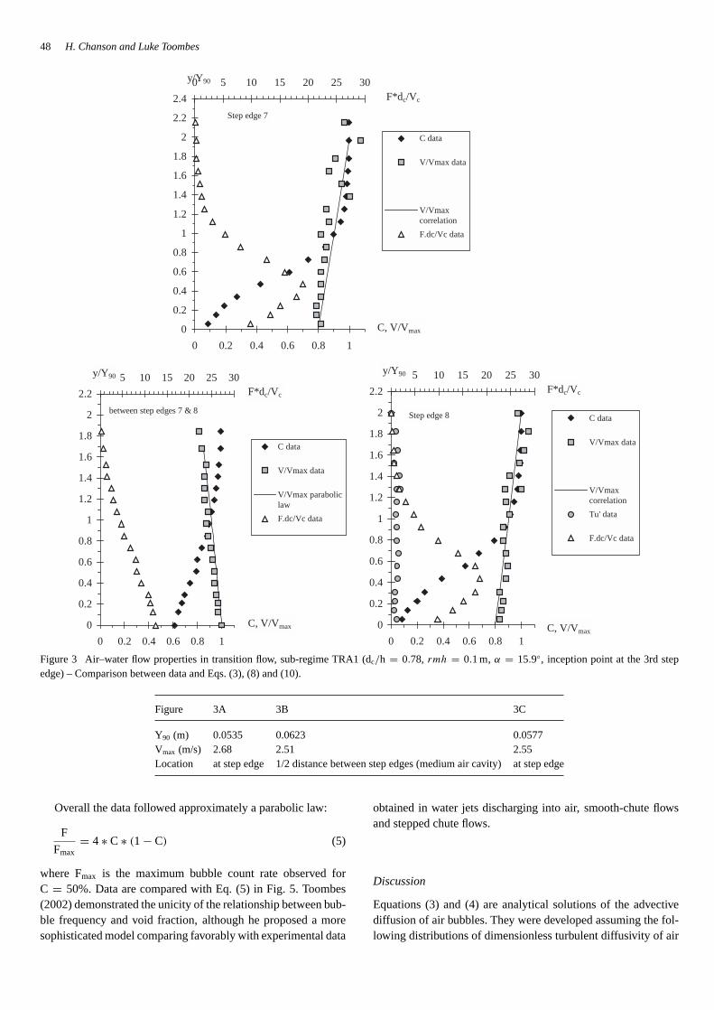
Figure 3 Air–water flow properties in transition flow, sub-regime TRA1 (dc/h = 0.78, rmh = 0.1 m, α = 15.9◦, inception point at the 3rd stepedge) – Comparison between data and Eqs. (3), (8) and (10).

Figure 3A 3B 3C

Y90 (m) 0.0535 0.0623 0.0577Vmax (m/s) 2.68 2.51 2.55Location at step edge 1/2 distance between step edges (medium air cavity) at step edge

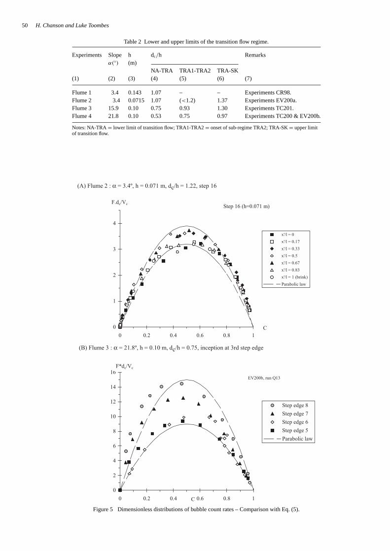
Overall the data followed approximately a parabolic law:

F

Fmax= 4 ∗ C ∗ (1 − C) (5)

where Fmax is the maximum bubble count rate observed forC = 50%. Data are compared with Eq. (5) in Fig. 5. Toombes(2002) demonstrated the unicity of the relationship between bub-ble frequency and void fraction, although he proposed a moresophisticated model comparing favorably with experimental data

obtained in water jets discharging into air, smooth-chute flowsand stepped chute flows.

Discussion

Equations (3) and (4) are analytical solutions of the advectivediffusion of air bubbles. They were developed assuming the fol-lowing distributions of dimensionless turbulent diffusivity of air

Hydraulics of stepped chutes: The transition flow 49

0

0.2

0.4

0.6

0.8

1

1.2

1.4

1.6

0 0.2 0.4 0.6 0.8 1

0 5 10 15 20 25 30

C data

V/Vmax data

V/Vmaxcorrelation

F.dc/Vc data

y/Y90

C, V/Vmax

step edge 7

F*dc/Vc

B

-0.3

-0.1

0.1

0.3

0.5

0.7

0.9

1.1

1.3

1.5

0 0.2 0.4 0.6 0.8 1

0 5 10 15 20 25 30

C data

V/Vmax data

V/Vmaxparabolic law

F.dc/Vc data

y/Y90

C, V/Vmax

between step edges 6 & 7

F*dc/Vc

A

-0.3

-0.1

0.1

0.3

0.5

0.7

0.9

1.1

1.3

1.5

1.7

1.9

0 0.2 0.4 0.6 0.8 1

0 5 10 15 20 25 30

C data

V/Vmax data

V/Vmaxparabolic law

F.dc/Vc data

y/Y90

C, V/Vmax

between edges 7 & 8

F*dc/Vc

C

0

0.2

0.4

0.6

0.8

1

1.2

1.4

1.6

1.8

0 0.2 0.4 0.6 0.8 1

0 5 10 15 20 25 30

C data

V/Vmax data

V/Vmaxcorrelation

F.dc/Vc data

y/Y90

C, V/Vmax

step edge 8

F*dc/Vc

D

Figure 4 Air–water flow properties in transition flow, sub-regime TRA2(dc/h = 1.06, h= 0.1 m,α = 15.9◦, inception point at the 4th step edge) –Comparison between data and Eqs. (4), (9) and (10).

Figure 4A 4B 4C 4D

Y90 (m) 0.0853 0.0677 0.0651 0.0648Vmax (m/s) 2.73 2.83 2.78 2.83Location 1/2 distance between step edges (large air cavity) at step edge 1/2 distance between step edges (filled cavity) at step edge

bubbles:

D′ = C ∗ √1 − C

λ ∗ (K ′′′ − C)Sub-regime TRA1 (6)

D′ = Do

1 − 2 ∗ (y/Y90 − 1/3)2Sub-regime TRA2 (7)

where D′ = Dt/((ur)Hyd ∗ cosα ∗ Y90), Dt is the turbulent diffu-sivity, (ur)Hyd is the rise velocity in hydrostatic pressure gradient

(Appendix). Note that the shape of Eq. (6) is similar to the sed-iment diffusivity distribution developed by Rouse (1937) whichyields to the Rouse distribution of suspended matter (e.g. Nielsen,1992; Chanson, 1999).

Velocity distributionsAir–water velocity measurements showed flat, straight velocityprofiles at step edges for all flow conditions and for y/Y90 < 2

50 H. Chanson and Luke Toombes

Table 2 Lower and upper limits of the transition flow regime.

Experiments Slope h dc/h Remarksα(◦) (m)

NA-TRA TRA1-TRA2 TRA-SK(1) (2) (3) (4) (5) (6) (7)

Flume 1 3.4 0.143 1.07 – – Experiments CR98.Flume 2 3.4 0.0715 1.07 (<1.2) 1.37 Experiments EV200a.Flume 3 15.9 0.10 0.75 0.93 1.30 Experiments TC201.Flume 4 21.8 0.10 0.53 0.75 0.97 Experiments TC200 & EV200b.

Notes: NA-TRA= lower limit of transition flow; TRA1-TRA2= onset of sub-regime TRA2; TRA-SK= upper limitof transition flow.

(A) Flume 2 : α = 3.4º, h = 0.071 m, dc/h = 1.22, step 16

0

1

2

3

4

0 0.2 0.4 0.6 0.8 1

x'/l = 0

x'/l = 0.17

x'/l = 0.33

x'/l = 0.5

x'/l = 0.67

x'/l = 0.83

x'/l = 1 (brink)

Parabolic law

C

Step 16 (h=0.071 m)F.dc/Vc

(B) Flume 3 : α = 21.8º, h = 0.10 m, dc/h = 0.75, inception at 3rd step edge

0

2

4

6

8

10

12

14

16

0 0.2 0.4 0.6 0.8 1

Step edge 8

Step edge 7

Step edge 6

Step edge 5

Parabolic law

C

EV200b, run Q13

F*dc/Vc

Figure 5 Dimensionless distributions of bubble count rates – Comparison with Eq. (5).

Hydraulics of stepped chutes: The transition flow 51

0

0.2

0.4

0.6

0.8

1

1.2

1.4

0 0.2 0.4 0.6 0.8 1

Run 1050, x/do=18

Run 1050, x/do=37

Run 1051, x/do=31

Run 1051, x/do=40

Correlation

y/Y90

V/V90

CHANSON (1988)

Figure 6 Dimensionless velocity distributions in the impact region downstream of a spillway aeration device (Data: Chanson, 1988) – Comparisonbetween data and Eq. (9).

(Figs. 3 and 4). It is believed that large energy dissipation at eachstep is associated with very-energetic turbulent mixing acrossthe entire air–water flow. In turn the strong momentum mixingyields quasi-uniform velocity profiles. Overall the data at stepedges were correlated by:

V

Vmax∼ 0.8 + 0.1 ∗

(y

Y90

)

sub-regime TRA1(y/Y90 < 2) (8)

V

Vmax∼ 0.95∗

(y

Y90+ 0.3

)0.07

sub-regime TRA2(y/Y90 < 1.6) (9)

Equations (8) and (9) are shown in Figs. 3A and C, and 4B andD respectively. They are very-rough estimate without theoreticalbackground. The velocity results differ significantly from skim-ming flow data: e.g. Matos (2000) and Chanson and Toombes(2001) observed a 1/5 to 1/6-th power law at step edges.

Velocity data in transition flows are somehow similar to (1)detailed air-water measurements immediately downstream ofnappe impact in nappe flows (Toombes, 2002) and to (2) air–water data in the impact region of spillway aeration deviceflows (Chanson, 1988). Figure 6 compares the latter set of datawith Eq. (9). Despite some scatter associated with the crudeinstrumentation, some agreement is seen.

At half-distance between step edges (Figs. 3B and 4A and C),the velocity distributions showed a marked change from obser-vations at step edges. The data were similar to ideal-fluid flowvelocity profiles in free-falling jet downstream of an overfall.Extending the reasoning of Montes (1998, p. 216), the velocitydistribution in the jet may be analytically derived as:

V

V90=

√1 − 2 ∗ y/Y90

Fr2

between step edges(for y/Y90 > 0) (10)

where Fr is the inflow Froude number at the upstream step edge.Equation (10) assumes an uniform velocity profile upstream ofjet take-off and neglects the effect of an upstream boundary layer.Figures 3B and 4A and C shows a close agreement betweenEq. (10) and the data (sub-regimes TRA1 and TRA2), includingabove a filled cavity (Fig. 4C).

Discussion

A characteristic feature of transition flow was the intense splash-ing and strong free-surface aeration which was observed on allslopes for all experiments. Figure 7 presents depth-averaged datashowing the mean air concentration Cmean as a function of thedimensionless distance x/dc from the upstream end of the chute.(Note the logarithmic scale of the horizontal axis.) Figure 7includes data measured at step edges and between step edges.The results show mean air contents larger then acknowledgedmean air concentrations in smooth-invert and skimming flows.For example, the re-analysis of Straub and Anderson’s (1958)data on smooth-inverts yields maximum (equilibrium) mean airconcentration of 0.07, 0.25 and 0.30 forα = 3.4◦, 16◦ and 22◦

respectively. Observed air contents in transition flows were abouttwice to three times larger (Fig. 7).

The flow resistance was estimated based upon air-water flowproperties measured at step edges. The Darcy friction factor wascalculated as

fe = 8 ∗ g

q2w

∗(∫ y=Y90

y=0(1 − C) ∗ dy

)3

∗ Sf (11)

where fe is the Darcy friction factor for air–water flow, g is thegravity acceleration, qw is the water discharge per unit width, Sf isthe friction slope(Ss = −∂H/∂x), H is the total head and x is thedistance in the flow direction. The results based upon total headdata calculated at step edges are summarised in Table 3 and theyare compared with flow resistance observations in nappe flows

52 H. Chanson and Luke Toombes

0

0.1

0.2

0.3

0.4

0.5

0.6

0.7

0.8

10 100 1000

dc/h = 1.22 (3.4 deg)

dc/h = 0.78 (16 deg)

dc/h = 1.06 (16 deg)

dc/h = 0.65 (22 deg)

dc/h = 0.87 (22 deg)

Cmean

x/dc

Figure 7 Longitudinal variations of the mean air concentration.

Table 3 Flow resistance estimates based upon detailed air–water flow measurements.

Ref. Flow regime dc/h fe Remarks(1) (2) (3) (4) (5)

Flume 1 Nappe flow 0.6–0.95 0.07–0.096 Single tip probe data. Experiments CR_98.Flume 2 Transition flow 1.22 0.029 Single-tip probe data. Experiments EV200a.

Skimming flow 1.5–1.9 0.034–0.042Flume 3 Transition flow 0.6–1.0 0.125–0.244 Single-tip and double-tip probe data. Experiments TC200 & EV200b.

Skimming flow 1.05–1.5 0.074–0.283Flume 4 Transition flow 0.78–1.06 0.105–0.107 Double-tip probe data. Experiments TC201.

Skimming flow 1.54 0.14

and skimming flows in the same facilities. Overall, the frictionfactor data in transition flows are comparable to flow resistancedata in skimming and nappe flows in the same facilities. For3.4 ≤ α ≤ 22◦, the flow resistance tends to increase with the bedslope as observed by Ohtsu andYasuda (1997) in skimming flows.

The strong flow aeration and relatively-slow flow velocity(compared to smooth chutes) yield large air–water interfacial areaand large residence times. Both contribute strong air–water masstransfer, and it is suggested that the transition flows might be asuitable flow regime to maximise air–water gas transfer down astepped cascade.

Conclusion

The present study demonstrates the existence of a transitory flowregime for intermediate flow rates between nappe and skimmingflows. The transition flow regime does not have the quasi-smoothfree-surface appearance of skimming flows, nor the distinctivesuccession of free-falling nappes observed in nappe flows. Itis characterised by a chaotic behaviour associated with intensesplashing and strong free-surface aeration.

The lower and upper limits of transition flows are presentedin Table 2 and Fig. 2. Detailed air–water flow measurements

highlight two sub-regimes. For low flow rates, the longitudinalflow pattern is characterised by irregular succession of small andlarge air cavities at each step, associated with almost linear airconcentration distributions (Fig. 3). For larger flow rates, somecavities are filled and the air concentration distributions have thesame shape as in skimming flows (Fig. 4).

Air–water velocity measurements showed nearly straight dis-tributions at step edges. It is proposed that strong turbulent mixingacross the flow contributes to quasi-uniform velocity profiles.Between step edges, the velocity distributions may be predictedby ideal-fluid calculations for free-falling nappes.

In summary the transition flows have very different character-istics from both nappe and skimming flows. Dominant featuresinclude intense droplet ejection and spray. Measured air contentswere two to three times larger than those recorded in smoothchutes and skimming flows, and the strong aeration might besuitable to enhance air–water gas transfer.

Acknowledgments

The authors acknowledge the assistance of M. Eastman, N. VanSchagen. The first writer thanks Dr Y. Yasuda and Professor I.Ohtsu for their helpful comments.

Hydraulics of stepped chutes: The transition flow 53

Appendix: Air bubble diffusion in transition flows

Free-surface aeration occurs when turbulence acting next to thefree-surface is large enough to overcome both surface tension forthe entrainment of air bubbles and buoyancy to carry downwardsthe bubbles. At uniform equilibrium, the air concentration dis-tribution is a constant with respect to the distance x in the flowdirection. The continuity equation for air in the air-water flowyields:

∂

∂y

(Dt ∗ ∂C

∂y

)= cosα ∗ ∂

∂y(ur ∗ C) (A.1)

where Dt is the air bubble turbulent diffusivity, ur is the bubble risevelocity,α is the channel slope and y is measured perpendicularto the mean flow direction. The bubble rise velocity in a fluid ofdensityρw ∗(1−C) equals: ur = (ur)Hyd∗√

1 − C where(ur)Hyd

is the rise velocity in hydrostatic pressure gradient (Chanson,1995b). A first integration of the continuity equation for air inthe equilibrium flow region leads to:

∂C

∂y′ = 1

D′ ∗ C ∗ √1 − C (A.2)

where y′ = y/Y90 and D′ = Dt/((ur)Hyd ∗ cosα ∗ Y90) is adimensionless turbulent diffusivity.

Chanson (1995b) solved Eq. (A.2) assuming a homoge-neous turbulence across the flow (i.e. D′ constant). Chansonand Toombes (2001) detailed further analytical models of voidfraction distributions assuming a non constant diffusivity D′.Results were successfully compared with transition and skim-ming air–water flow data. Toda and Inoue (1997) developedtwo-dimensional numerical models of the advective diffusionequation for air bubbles. The results of both Lagrangian andEulerian models gave very similar results to air-water flow mea-surements and to the analytical models of Chanson and Toombes(2001).

Notations

C = air concentration defined as the volume of air per unitvolume, also called void fraction

Cmean= depth averaged air concentration defined as: Cmean =1

Y90∗ ∫ Y90

y=0 C ∗ dy

Dt = turbulent diffusivity (m2/s) of air bubble in air–waterflows

Do = dimensionless coefficientD′ = dimensionless air bubble diffusivity (defined by

Chanson, 1995b)dc = critical flow depth (m); for a rectangular channel: dc =

3√

q2w/g

do = inflow depth (m)F = bubble count rate (Hz): i.e. number of bubbles detected

by the probe sensor per secondFmax = maximum bubble count rate (Hz)

Fr = Froude numberfe = Darcy friction factor of air–water flowsg = gravity constant (m/s2); g = 9.80 m/s2 in

BrisbaneH = total head (m)h = height of steps (m) (measured vertically)

K ′, K ′′, K ′′′ = integration constantsL = chute length (m)l = horizontal length of steps (m) (measured perpen-

dicular to the vertical direction)qw = water discharge per meter width (m2/s)Sf = friction slopeur = bubble rise velocity (m/s)

(ur)Hyd = bubble rise velocity (m/s) in a hydrostatic pressuregradient

V = air–water velocity (m/s)Vc = critical velocity (m/s); for a rectangular channel:

Vc = 3√

g ∗ qw

Vmax = maximum velocity (m/s)W = chute width (m)x = longitudinal distance (m)x′ = horizontal distance (m) measured from the verti-

cal step facey = 1 – distance (m) from the bottom measured

perpendicular to the spillway invert= 2 – distance (m) from the pseudo-bottom (formed

by the step edges) measured perpendicular to theflow direction

Greek symbolsα = channel slopeλ = dimensionless coefficient� = diameter (m)

Subscriptc = critical flow conditions

References

1. BaCaRa (1991). “Etude de la Dissipation d’Energie surles Evacuateurs à Marches.” (‘Study of the Energy Dis-sipation on Stepped Spillways.’)Rapport d’Essais, ProjetNational BaCaRa, CEMAGREF-SCP, Aix-en-Provence,France, Oct., 111 pages (in French).

2. Beitz, E. and Lawless, M. (1992). “Hydraulic ModelStudy for dam on GHFL 3791 Isaac River at Burton Gorge,”Water Res. Commission Report, Ref. No. REP/24.1, Sept.,Brisbane, Australia.

3. Boes, R.M. (2000). “Zweiphasenstroömung und Energieum-setzung an Grosskaskaden.” (‘Two-Phase Flow and EnergyDissipation on Cascades.’)PhD thesis, VAW-ETH, Zürich,Switzerland (in German). (alsoMitteilungen der Ver-suchsanstalt fur Wasserbau, Hydrologie und Glaziologie,ETH-Zurich, Switzerland, No. 166).

4. Bos, M.G. (1976). “Discharge Measurement Structures,”Publication No. 161, Delft Hydraulic Laboratory, Delft, The

54 H. Chanson and Luke Toombes

Netherlands (also Publication No. 20, ILRI, Wageningen,The Netherlands).

5. Chamani, M.R. and Rajaratnam, N. (1999). “Onset ofSkimming Flow on Stepped Spillways,”J. Hydr. Engrg.ASCE, 125(9), 969-971. Discussion: 127(6), 519–525.

6. Chanson, H. (1988). “A Study of Air Entrainment andAeration Devices on a Spillway Model,”PhD thesis, Ref.88-8, Dept. of Civil Engrg., University of Canterbury, NewZealand (ISSN 0110-3326).

7. Chanson, H. (1995a). “Predicting the Filling of VentilatedCavities behind Spillway Aerators,”J. Hydr. Res. IAHR,33(3), 361–372.

8. Chanson, H. (1995b). “Air Bubble Diffusion in Supercrit-ical Open Channel Flow,”Proc. 12th Australasian FluidMechanics Conference AFMC, Sydney, Australia, R.W.BILGER Ed., Vol. 2, pp. 707–710 (ISBN 0 86934 034 4).

9. Chanson, H. (1996). “Prediction of the TransitionNappe/Skimming Flow on a Stepped Channel,”J. Hydr. Res.IAHR, 34(3), 421–429 (ISSN 0022-1686).

10. Chanson, H. (1999). “The Hydraulics of Open ChannelFlows: An Introduction,” Butterworth-Heinemann, Oxford,UK, 512 pages.

11. Chanson, H. and Toombes, L. (1998). “Supercritical Flowat an Abrupt Drop: Flow Patterns and Aeration,”Can. J.Civil Engrg., 25(5), 956–966.

12. Chanson, H. and Toombes, L. (2001). “ExperimentalInvestigations of Air Entrainment in Transition and Skim-ming Flows down a Stepped Chute. Application to Embank-ment Overflow Stepped Spillways,”Research Report No.CE158, Dept. of Civil Engrg., University of Queensland,Brisbane, Australia, July.

13. Chanson, H., Yasuda, Y. and Ohtsu, I. (2000). “FlowResistance in Skimming Flow: A Critical Review,”Int.Workshop on Hydraulics of Stepped Spillways, Zürich,Switzerland, H.E. Minor and W.H. Hager Eds., BalkemaPubl., pp. 95–102 (ISBN 90 5809 135X).

14. Elviro, V. and Mateos, C. (1995). “Spanish Researchinto Stepped Spillways,”Int. J. Hydropower & Dams, 2(5),61–65.

15. Haddad, A.A. (1998). “Water Flow Over Stepped Spill-way,” Masters Thesis, Polytechnic of Bari, Italy.

16. Henderson, F.M. (1966). “Open Channel Flow,”MacMillan Company, New York, USA.

17. Horner, M.W. (1969). “An Analysis of Flow on Cascadesof Steps,”PhD thesis, Univ. of Birmingham, UK, May, 357pages.

18. Matos, J. (2000). “Hydraulic Design of Stepped Spillwaysover RCC Dams,”Int. Workshop on Hydraulics of SteppedSpillways, Zürich, Switzerland, H.E. Minor and W.H. HagerEds., Balkema Publ., pp. 187–194.

19. Matos, J. (2001). “Onset of Skimming Flow on SteppedSpillways. Discussion,”J. Hydr. Engrg.ASCE, 127(6), 519–521.

20. Montes, J.S. (1994). Private Communication.21. Montes, J.S. (1998). Hydraulics of Open Channel Flow.

ASCE Press, New York, USA, 697 pages.22. Nielsen, P. (1992). “Coastal Bottom Boundary Layers and

Sediment Transport,”Advanced Series on Ocean Engrg.,Vol. 4, World Scientific Publ., Singapore.

23. Ohtsu, I. and Yasuda, Y. (1997). “Characteristics of FlowConditions on Stepped Channels,”Proc. 27th IAHR BiennalCongress, San Francisco, USA, Theme D, pp. 583–588.

24. Ohtsu, I., Yasuda, Y. and Takahashi, M. (2001). “Onsetof Skimming Flow on Stepped Spillways. Discussion,”J. Hydr. Engrg. ASCE, 127(6), 522–524.

25. Pinheiro, A.N. and Fael, C.S. (2000). “Nappe Flow inStepped Channels – Occurrence and Energy Dissipation,”Int. Workshop on Hydraulics of Stepped Spillways, Zürich,Switzerland, H.E. Minor and W.H. Hager Eds„ BalkemaPubl., pp. 119–126.

26. Rajaratnam, N. (1990). “Skimming Flow in Stepped Spill-ways,”J. Hydr. Engrg. ASCE, 116(4), 587–591. Discussion:118(1), 111–114.

27. Rouse, H. (1937). “Modern Conceptions of the Mechanicsof Turbulence,”Transactions ASCE, 102, 463–543.

28. Ru, S.X., Tang, C.Y., Pan, R.W. and He, X.M. (1994).“Stepped Dissipator on Spillway Face,”Proc. 9th APD-IAHR Congress, Singapore, Vol. 2, pp. 193–200.

29. Shi, Q., Pan, S., Shao, Y. and Yuan, X. (1983). “Experi-mental Investigation of Flow Aeration to prevent CavitationErosion by a Deflector,”Shuili Xuebao (J. Hydr. Engrg.),Beijing, China, 3, 1–13 (in Chinese).

30. Shvajnshtejn, A.M. (1999). “Stepped Spillways andEnergy Dissipation,”Gidrotekhnicheskoe Stroitel’stvo, No.5, pp. 15–21 (in Russian). (AlsoHydrotechnical Construc-tion, 3(5), 1999, 275–282.)

31. Stephenson, D. (1979). “Gabion Energy Dissipators,”Proc. 13th ICOLD Congress, New Delhi, India, Q. 50, R. 3,pp. 33–43.

32. Straub, L.G. and Anderson, A.G. (1958). “Experimentson Self-Aerated Flow in Open Channels,”J. Hydr. Div. Proc.ASCE, 84(HY7), 1890-1–1890-35.

33. Toda, K. and Inoue, K. (1997). “Advection and Diffusionproperties of Air Bubbles in Open Channel Flow,”Proc.27th IAHR Congress, San Francisco, USA, Theme B, F.M.Holly Jr. and A. Alsaffar Ed., Vol. 1, pp. 76–81.

34. Toombes, L. (2002). “Experimental Study of Air–WaterFlow Properties on low-gradient Stepped Cascades,” Ph.D.thesis, Dept of Civil Engrg., University of Queensland,Brisbane, Australia.

35. Yasuda, Y. and Ohtsu, I.O. (1999). “Flow Resistance ofSkimming Flow in Stepped Channels,”Proc. 28th IAHRCongress, Graz, Austria, Session B14, 6 pages.