San Jose State University San Jose State University

SJSU ScholarWorks SJSU ScholarWorks

Master's Theses Master's Theses and Graduate Research

Spring 2018

Hydraulic Sheet Resistance In Paper-Based Porous Media Hydraulic Sheet Resistance In Paper-Based Porous Media

Stefan Myles Doser San Jose State University

Follow this and additional works at: https://scholarworks.sjsu.edu/etd_theses

Recommended Citation Recommended Citation Doser, Stefan Myles, "Hydraulic Sheet Resistance In Paper-Based Porous Media" (2018). Master's Theses. 4900. DOI: https://doi.org/10.31979/etd.fba3-492g https://scholarworks.sjsu.edu/etd_theses/4900

This Thesis is brought to you for free and open access by the Master's Theses and Graduate Research at SJSU ScholarWorks. It has been accepted for inclusion in Master's Theses by an authorized administrator of SJSU ScholarWorks. For more information, please contact scholarworks@sjsu.edu.

HYDRAULIC SHEET RESISTANCE IN PAPER­BASED POROUS MEDIA

A Thesis

Presented to

The Faculty of the Department of Mechanical Engineering

San José State University

In Partial Fulfillment

of the Requirements for the Degree

Master of Science

by

Stefan M. Doser

May 2018

© 2018

Stefan M. Doser

ALL RIGHTS RESERVED

The Designated Thesis Committee Approves the Thesis Titled

HYDRAULIC SHEET RESISTANCE IN PAPER­BASED POROUS MEDIA by

Stefan M. Doser

APPROVED FOR THE DEPARTMENT OF MECHANICAL ENGINEERING

SAN JOSÉ STATE UNIVERSITY

May 2018

Sang­Joon (John) Lee, Ph.D. Department of Mechanical Engineering

Matuesz Bryning, Ph.D. Chief Technology Officer, Zikon, Inc.

Mark Sullivan, M.S. Lead Engineer, Oculus, Inc.

ABSTRACT

HYDRAULIC SHEET RESISTANCE IN PAPER­BASED POROUS MEDIA

by Stefan M. Doser

This work investigates the special case of in­plane fluid flow of a Newtonian

incompressible fluid across a thin paper­based porous medium at very low Reynolds

numbers (Re ≪ 1). Fluid transport with these characteristics is used in emerging devices

such as microscale paper­based analytical devices ( µ PADs). The mathematical similarity

between Darcy’s law and Ohm’s law is considered, and hydraulic equivalents of current,

voltage and resistance are determined to propose hydraulic sheet resistance. Darcy flow

is predicted under these conditions and tested by experiment at two flow rates of 5 µL/min

and 10 µL/min. A device was designed and fabricated to ensure a deterministic 310 μm

gap that directs prescribed flow, unidirectionally across Grade 50 Whatman filter paper.

Pressure was measured along the direction of flow over a 125 mm distance at six pressure

ports placed at uniform increments of 25 mm. Measurements were recorded over a time

period up to 48 hours at discrete intervals with at least four replicates. Measurements of

the pressure profile showed a linear relationship as predicted by Darcy’s law, which allow

hydraulic permeability, hydraulic bulk resistivity and hydraulic sheet resistivity to be

calculated as 324 mm 2 , 2995 s ­1 and 9433 (mm⋅s) ­1 respectively. Among replicates

measured under the same set of controllable experimental conditions, the data also show

a nonlinear relationship, suggesting transition into a nonlinear flow regime dependent

upon inlet pressure and media tortuosity.

ACKNOWLEDGMENTS

This work was supported in part by the Davidson Student Scholars Program of the

Charles W. Davidson College of Engineering at San José State University. Scanning

electron microscope images provided by San José State University. I would like to thank

Dr. Matuesz Bryning for his support in the subject of porous media and enthusiasm for

the theoretical work involved. I would like to thank Professor Mark Sullivan for his

support with kinematic design and help as a coordinate measurement machine operator. I

would like to thank Dr. Sang­Joon (John) Lee for his continuous support throughout this

project with countless hours of advise and review. Finally, I would like to thank my

friends, family and wife Veronica for their support and often needed distraction.

v

TABLE OF CONTENTS LIST OF TABLES…………………………………………………………………. ix LIST OF FIGURES ……………………………………………………………….. x LIST OF SYMBOLS AND ABBREVIATIONS …………………………………. xi 1. INTRODUCTION………………………………………………………………. 1

1.1 Background ………………………………………………………………. 1 1 .1.1 Consideration and Selection of Fluid ………………………………. 2 1 .1.2 Consideration and Selection of Porous Media ………………………. 3

1.2 Hypothesis …………………………………………………………………. 4 1.3 Significance ………………………………………………………………. 5

2 . THEORY ………………………………………………………………………. 6 2 .1 Darcy’s Law ………………………………………………………………. 6 2 .2 Review of the Four­Point Probe Method …………………………………. 10 2 .3 Defining Electrical Sheet Resistance………………………………………. 12 2 .4 Applying Darcy’s Law to Sheet Resistance ………………………………. 15

3 . RELATED WORK………………………………………………………………. 21 3 .1 Flow Regimes within Porous Media ………………………………………. 21

3 .1.1 Flow Regime Identification Criteria…………………………………. 21 3 .1.2 The Weak Inertia Regime……………………………………………. 23 3 .1.3 The Forchheimer Regime……………………………………………. 24 3 .1.4 The Turbulent Regime ……………………………………………… 26

3 .2 Explanations for Non­Darcy Flow in Porous Media………………………. 27 3 .2.1 Inertial Effects as a Contributor to Non­Darcy Flow ………………. 27 3 .2.2 Porous Media Qualities as a Contributor to Non­Darcy Flow ………. 27

3 .3 Boundary Condition Effects in Porous Media Flow ………………………. 28 3 .4 Paper­Based Porous Media Flow Device Research ………………………. 29

3 .4.1 Current Application of Paper­Based Porous Media …………………. 29 3 .4.2 Time­Delay Research in Paper­Based Porous Media ………………. 30 3 .4.3 Flow Control Research in Paper­Based Porous Media………………. 31

4. METHODOLOGY………………………………………………………………. 33 4.1 Selection of Paper Media and Sample Preparation ………………………. 33 4.2 Design of the Hydraulic Resistance Tester ………………………………. 35

4.2.1 Functional Requirements ……………………………………………. 35 4.2.2 Kinematic Design and Construction…………………………………. 36

vi

4. 3 Fluid Flow Rate Device and Tube Selection ………………………………. 37 4. 4 Pressure Measurement Methodology………………………………………. 39

4.4.1 Determining Pressure in Porous Media ……………………………. 39 4.4.2 Pressure Measurement Selection ……………………………………. 39

4.5 Experimentation……………………………………………………………. 42 4.5.1 Experimental Preparation ……………………………………………. 42 4.5.2 Experimental Conditions ……………………………………………. 42

4.6 Sources of Uncertainty ……………………………………………………. 44 4.6.1 Relative and Combined Error ………………………………………. 44 4.6.2 Unquantified Uncertainty ……………………………………………. 46

5. RESULTS AND DISCUSSION ………………………………………………. 49 5 .1 Collected Data ……………………………………………………………. 49

5 .1.1 Best Data Representation ……………………………………………. 49 5 .1.2 Linear and Nonlinear Determination ………………………………. 51

5 .2 Analysis ……………………………………………………………………. 53 5 .2.1 Curve Fit Equations …………………………………………………. 53 5 .2.2 Special Observations and Explanations ……………………………. 55 5 .2.3 Calculated Material Properties ………………………………………. 58

6. CONCLUSIONS ………………………………………………………………. 61 6 .1 Addressing the Hypothesis…………………………………………………. 61 6 .2 Discoveries from Experimentation ………………………………………. 61 6 .3 Recommendations for Future Work ………………………………………. 62

6 .3.1 Recommendations for Methodology…………………………………. 62 6 .3.2 Recommendations for Testing ………………………………………. 63

REFERENCES CITED ……………………………………………………………. 65 APPENDIX A: APPARATUS TECHNICAL DOCUMENTS……………………. 74

Bill of Material…………………………………………………………………. 74 Top Plate 2D……………………………………………………………………. 75 Bottom Plate 2D ………………………………………………………………. 76

APPENDIX B: COORDINATE MEASUREMENT MACHINE FLATNESS…… 77 Coordinate Measurement Machine Bottom Bracket …………………………. 77 Coordinate Measurement Machine Top Bracket Main ………………………. 78 Coordinate Measurement Machine Top Bracket Edges ………………………. 79

APPENDIX C: EXPERIMENTAL RAW DATA CHARTS………………………. 80 Pressure Readings Separated by Location Over Time…………………………. 80

vii

Pressure Readings Separated by Time over Location …………………………. 82

Curve Fitted Pressure Readings Over Location at One Instance………………. 84

viii

LIST OF TABLES

Table 1.

Summary of uncertainty as relative error for permeability k calculation……………………………………………………………. 46

Table 2. Maximum pressure, linear regression fit values for flow at 10 µL/min

and 5 µL/min…………………………………………………………. 53

Table 3. Flow rate, coefficients and regression fit values for data sets fitted by

equation (54)…………………………………………………………. 54

Table 4. Flow rate, coefficients and regression fit values for data sets fitted by

equation (54)…………………………………………………………. 55

Table 5. Flow rate and calculated material permeability k (mm 2 ) from equation (51) of linear data sets………………………………………………... 59

ix

LIST OF FIGURES

Figure 1.

Diagram of the four­point probe method on a surface with the outer

probes………………………………………………………………….

11

Figure 2. A representation of the hypothetical current density field assumed in

electrical sheet resistance definition………………………………….. 13

Figure 3. A representation of the hypothetical flow density field from inlet to

outlet with…………………………………………………………….. 18

Figure 4. Scanning electron microscope (SEM) image of grade 50 Whatman

filter paper…………………………………………………………….. 34

Figure 5. Data set 5 pressure readings separated by measurement location as a

function of time……………………………………………………….

49

Figure 6. Data set 5 pressure readings as a function of distance from inlet to

outlet, measured at……………………………………………………. 50

Figure 7. Data set 5 at hour 24.75 showing individual pressure readings and a

curve………………………………………………………………….. 51

Figure 8. Data set 2 at hour 25 showing individual pressure readings and a

curve fitting the data as………………………………………………. 52

Figure 9. Data set 9 at hour 23 showing individual pressure readings and a

curve fitting the data as………………………………………………. 56

Figure 10. Data set 10 at hour 25 showing individual pressure readings and a

curve fitting the data as………………………………………………. 56

Figure 11. Data set 6 at hour 46.50 showing individual pressure readings and a

curve fitting the data as………………………………………………. 57

Figure 12. Maximum recorded pressure drop for linear pressure profile data sets

(1, 2, 6, 7 & 8)……………………………………………………….. 58

Figure 13. Maximum recorded pressure drop for linear pressure profile data sets

(3, 4, 5, 9 & 10)……………………………………………………… 59

x

LIST OF SYMBOLS

Symbol Description ________________________________________________________________________

a Placeholder constant A Area (m 2 ) A Regression fit constant b Placeholder constant B Regression fit constant C Regression fit constant d Average particle diameter (m) d p Pore diameter (m) d part Particle diameter (m) D Diameter of porous media bed (m) D Regression fit constant E Vector of electromagnetic field force (volt/m) F Vector of flow field force (m/s 2 ) g Scaler force of gravity (m/s 2 ) G Vector of gravitational force (m/s 2 ) h Height above elevation datum (m) h 1 First manometer height (m) h 2 Last manometer height (m) i Current density (A/m 2 ) i Vector of current density field (ampere/m 2 ) I Current (ampere) k Darcy permeability coefficient (m 2 ) k f Forchheimer permeability coefficient (m 2 ) K Darcy’s hydraulic conductivity K′ Remainder of Darcy’s hydraulic conductivity l Length (m) L Length of flow path (m) n A finite number of terms in a series N Dimensionless factor of proportionality P Pressure (Pa) q Flow density (m/s) q Vector of flow density field (m/s) Q Volume flow rate (m 3 /s) r Radius (m) R Electrical resistance (Ω) R h Hydraulic resistance (m/s)

xi

Re Reynolds number

Re m Modified Reynolds number

Re p Pore Reynolds number

s Probe spacing (m)

S part Particle surface area (m 2 )

t Thickness (m)

u Range of uncertainty

v p Pore velocity (m/s)

V Voltage (V)

V part Particle volume (m 3 )

w Width (m)

x Linear distance (m)

X Dimensionless inertial contribution ratio

y Source of uncertainty

z Height direction parallel to gravity (m)

Inertial resistance coefficient

Weak inertia coefficient

Dimensionless voidage in porous media

Dynamic fluid viscosity (Pa·s)

Fluid density (kg/m 3 )

a Particle apparent density (kg/m 3 )

b Electrical bulk resistivity (Ω·m)

bulk Particle bulk density (kg/m 3 )

s Electrical sheet resistivity (resistance) (Ω/)

Hydraulic conductivity (s)

e Electromagnetic conductivity (Ω ­1 ·m

­1 )

b Hydraulic bulk resistivity (s ­1 )

s Hydraulic sheet resistivity (resistance) (m ­1 ·s

­1 )

Φ Energy per unit mass (m 2 /s 2 )

xii

1. INTRODUCTION

1.1 Background

The concept of hydraulic resistance as it applies to the hydraulic­electrical analogy

has been established in research going back since the industrial revolution. The

theoretical framework for the hydraulic­electrical analogy can be seen in continuum

mechanics equations such as the Hagen­Poiseuille relation for cylindrical ducts, or

alternatively by manipulation of the Navier­Stokes equations for a direct albeit

cumbersome solution. However, the hydraulic­electrical analogy can be attributed in part

to Henry Darcy and a relationship he discovered known as Darcy's law. Simply put,

closed hydraulic systems function similarly to electrical circuits with hydraulic

equivalents of voltage, current and resistance which behave linearly with respect to

impetus and flow.

This work explores the hydraulic electrical analogy and applies it to the concept of

electrical sheet resistance which is widely used in the semiconductor manufacturing

industry. A notable departure from the classical hydraulic­electrical analogy is the

inclusion of porous media, which introduces additional considerations to the flow

dynamics. The inclusion of porous media requires observance to specific theoretical

frameworks but within this work remains the subject of incompressible low Reynolds

number flow of a Newtonian fluid.

1

An important distinction between the microfluidic experimental model tested in this

work and the industrial application of electrical sheet resistance is the aspect ratio of

sheet length and width relative to the thickness. In this work, empirical data are obtained

with aspect ratios of approximately 500:1 where electrical sheet resistance is often

measured at aspect ratios of 10000:1 or greater. Herein, an expanded discussion is

presented as to other similarities and differences between the microfluidic model and

electrical sheet resistance to explore how the behavior of hydraulic sheet resistance may

behave as understood by Darcy’s law.

1.1.1 Consideration and Selection of Fluid

Although gases and liquids are both of interest for porous media flow, the scope of

this study is limited to liquids. An important advantage of liquids is that they are nearly

completely incompressible. Gas, by contrast, is a compressible fluid which in a closed

system can exhibit non­steady state behavior with respect to flow rate and pressure.

Choosing an incompressible fluid ensures that any kind of harmonic behavior can be

ignored as a source of error, provided that the liquid delivery is steady without pressure

transients.

The chosen liquid is water. In addition to being isotropic, water is a Newtonian fluid

meaning that the viscous stress and strain rate are not dependent on the stress state of

velocity of flow but solely on temperature [1]. This is an important consideration

because viscosity directly contributes to hydraulic resistance as predicted by Darcy’s law.

2

For these reasons, water is an ideal candidate as a fluid for study. In addition, choosing

distilled or deionized water is most preferred because it ensures a minimum number of

particles within the water. These particulates can cause contamination of the porous

medium that will affect the hydraulic sheet resistance throughout experimentation.

1.1.2 Consideration and Selection of Porous Media

For this study, only a few media were considered for use. One option is the same

porous medium of the related work involving reverse­emulsion electrophoretic displays

or (REED) technologies which uses spray­deposited powder titanium dioxide [2].

However, this can be cost prohibitive and introduces other unwanted factors such as the

particle size variation, nonuniform agglomeration and repeatability of the deposited

material.

Another consideration is an unbound porous medium such as sand, similar to the

original medium studied by Darcy. However, sand is not as applicable within the field of

microelectromechanical devices because of the large pore size relative to the channel and

gap widths typically found in these devices. In addition, preference is given to fixed

matrix porous media over a media composed of free particles which can exhibit

unwanted behavior such as rearrangement and nonuniform channeling of fluid.

These considerations leave fibrous materials such as cellulose paper­based media as

preferred subjects for study. Not only are these porous media constrained within a

matrix, but these materials can be easily manufactured with tight dimensional thickness

3

tolerances of approximately ± 15 μm, and consistent porosity as in the case of the porous

media studied in previous work [3]. In addition, because paper is easy to manufacture,

such sheets are also inexpensive making paper­based media ideal for disposable

microdevices [4].

1.2 Hypothesis

This work investigates the special case of lateral fluid flow of a Newtonian

incompressible fluid across thin paper­based porous medium in a confined conduit. For

this case, the hypothesis is that pressure drop will behave linearly (i.e., as in Darcy flow)

with distance along the porous medium, for Reynolds numbers that are much less than

one (Re ≪ 1).

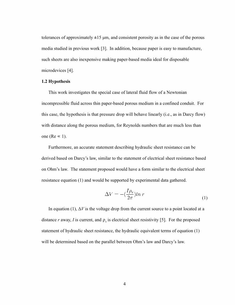
Furthermore, an accurate statement describing hydraulic sheet resistance can be

derived based on Darcy’s law, similar to the statement of electrical sheet resistance based

on Ohm’s law. The statement proposed would have a form similar to the electrical sheet

resistance equation (1) and would be supported by experimental data gathered.

(1)

In equation (1), Δ V is the voltage drop from the current source to a point located at a

distance r away, I is current, and s is electrical sheet resistivity [5]. For the proposed

statement of hydraulic sheet resistance, the hydraulic equivalent terms of equation (1)

will be determined based on the parallel between Ohm’s law and Darcy’s law.

4

1.3 Significance

There is still much to be discovered in the field of porous media flow and the

mechanisms that contribute to flow regime condition. Understanding this behavior by

exploring alternative theoretical frameworks can lead to advancement in fields that use

this technology. It is becoming more common for thin paper­based porous media to be

used in biomedical fluidic devices and thus it is important to understand if the special

case of thin porous media flow requires a correction to the pressure and flow rates

predicted by Darcy’s law [4]. One immediate application of this work is to predict

permeability of a common fluidic device materials. This is useful in the display

technology field which uses manufactured and deposited materials. Hydraulic sheet

resistance can be used as a quality control criterion to determine a medium’s permeability

in mass production. Alternatively, it can be used as a design criterion to determine the

time for an image to resolve as well as the stability of an image [2].

5

2. THEORY

2.1 Darcy’s Law

The study of porous media goes back to the mid 1800s with the first studies focused

on the fluid mechanics of flow through bulk porous material determined directly from

experimentation. In the years since, many have attempted to connect these observations

to a theoretical framework. This section will focus on these first observations by Darcy

and a theoretical framework that can be applied.

The study of flow through porous media began with Darcy’s law published by Henry

Philibert Gaspard Darcy in his book Les Fontaines Publiques de la Ville de Dijon in 1856

[6]. Darcy’s law was developed based on the study of hydrology as it applied to

groundwater behavior and the design of aquifers. Darcy’s law describes volume flow rate

Q as a function of the cross­sectional area of porous media normal to flow A , the

“hydraulic conductivity” K , the change in manometer height reading h where subscripts 1

and 2 denote inlet and outlet flow respectively, and the length of the flow path L as shown

in equation (2) below [7].

(2)

This relationship in (2) was found based on a series of experiments through a porous

medium with a known flow rate and the pressure drop from inlet to outlet recorded,

similar to the experiments done in this thesis to determine hydraulic sheet resistance.

6

Because Darcy’s law is based solely on empirical evidence, it lacks a satisfactory

connection to a greater physical theory of continuity as some may describe as a

“mass­point” or “microscopic” approach [8]. As such, many investigators have

attempted to relate Darcy’s law to one of these theories with varying degrees of success.

Because Darcy’s law is essential to this paper’s topic, some focus will be placed on the

most notable of these derivations to give an adequate background on this theory for

proper context.

First we must change the form of Darcy’s law so that we can relate physical and

dynamical parameters to field forces. This transformation is first done by experiment to

confirm that Darcy’s law is invariant of earth’s gravitational field with respect to flow

direction. We can visualize a field in three­dimensional space where at any point there

exists a scalar value h defined by the height above an elevation datum with respect to

which the flow moves perpendicularly. We can breakdown Darcy’s law into flow rate Q

divided by the cross­sectional area A, as a ratio called flow density q .

(3)

The flow density represents an impetus in the direction of flow, while still being

dependent on the manometer head (∇ h ), and a generalized impedance term K which

remains a lumped parameter capturing both physical and geometric conditions [7].

(4)

7

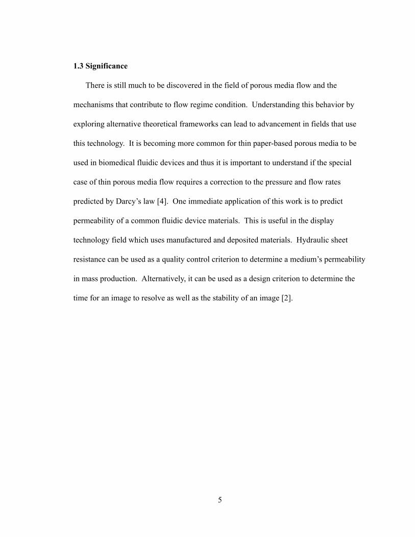
From the K term we can extract fluid density and dynamic viscosity μ , as well as an

average particle diameter d and dimensionless factor of proportionality N which captures

the geometry of the paths through the porous media [7]. The K′ accounts for any missed

terms from the lumped parameter K .

(5)

We can now address the impetus term by relating the manometer height to the hydrostatic

equation for pressure P ,

(6)

thus allowing us to express the gradient of h in terms of pressure and a height z above a

reference datum. Gravitational acceleration is represented by the customary variable g .

(7)

By multiplying both sides by g we can rewrite the expression as below.

(8)

The last term is the force of gravity pointing downward towards the earth and can be

re­expressed as vector G .

(9)

Now we can change the expression for the impetus of flow to the below.

(10)

8

The terms on the right­hand side of the equation express direction and magnitude of

the force applied upon a unit mass of fluid by both gravity and the gradient of fluid

pressure in the direction of flow. Another insight is that the gravitational term g is the

final concealed term of K′ [7]. Now that we can equate the manometer height to physical

forces, we will continue to use the left side of equation (10) and move the scalar g term

inside the gradient operation as below.

(11)

In this expression the ( gh ) term represents the work required to elevate a unit mass of

matter from the elevation datum to the height h in the manometer. It follows that,

(12)

where the expression can be viewed as the energy per unit mass or potential Φ. A more

complete expression for the energy per unit mass is,

(13)

which shows the additional contribution from the pressure field [7]. Now the expression,

(14)

is the intensity of the force field F acting upon the fluid. Finally, we can combine

equations (5), (11), (12) and (14) to re­express Darcy’s law within the context of physical

properties and field­forces.

(15)

9

Where the hydraulic bulk conductivity σ of the system is given by,

(16)

Hydraulic bulk conductivity has the units of seconds. When we compare this version of

Darcy’s law in (15) to Ohm’s law, we can see the parallel between them.

Darcy’s law: (17)

Ohm’s law: (18)

In Ohm’s law i is the current density, σ e is the electrical conductivity, E is the

electromagnetic field force, and V is the electrical potential [7].

With a more complete theoretical analogy between hydraulic and electrical behavior

based on physical properties and forces, we can examine the theory of electrical sheet

resistance and attempt to apply Darcy’s law to propose a theory of hydraulic sheet

resistance.

2.2 Review of the Four­Point Probe Method

The discussion of the four­point probe method and electrical sheet resistance are

nearly inseparable as the theory of electrical sheet resistance comes from this testing

method. Originally, the four­point probe method was used to test the resistivity of the

earth as described in a paper published in 1915 by Frank Wenner. In this paper Wenner

describes submerging four probes at regular distances in­line in the ground where the

outer two probes are an anode and cathode that conduct current past the inner two probes

that measure the electrical potential [9]. With this setup Wenner was able to

10

experimentally determine the resistivity of the soil in much the same way Darcy was able

to measure hydraulic resistivity sixty years earlier.

Later in 1954, L.B. Valdes wrote a paper describing the application of the four­point

probe method on the surface of germanium crystals of various geometries and positions

relative to boundary conditions. Valdes’ work covers experimental test scenarios along

with the mathematical expressions for predicting electrical resistivity for each case. One

such case is measuring the surface of a germanium crystal slab with a thickness

approximately equal to or greater than the spacing of the probes [10]. Figure 1 shows

this four­point probe setup on a conductive surface.

Figure 1. Diagram of the four­point probe method on a surface with the outer probes conducting current and the inner probes reading the potential difference.

11

Uhlir Jr. adds to this research with the insight that testing progressively thinner slabs

requires a larger correction divisor in order to calculate the electrical resistivity. Uhlir

concludes that this is more desirable in the statement,

“In general, a large correction divisor is desirable because it indicates that

a relatively large potential difference is to be measured. For this reason,

the use of the four­point probe on thin slices should be and, in fact, is

found in practice to be quite satisfactory [11].”

In 1957 the the four­point probe method was applied to thin sheets in a paper

authored by F.M. Smits. Smits expands the work of Valdes and Uhlir of four­point probe

testing to an infinite sheet with a relatively small thickness compared to probe spacing.

From this, Smits makes reference to sheet resistivity as a function of distance of dipoles

and formally defines sheet resistance [5].

2.3 Defining Electrical Sheet Resistance

Although not explicitly derived in Smits’ work, a complete description can be shown

by application of Ohm’s law and visualizing the current density field approximated as an

expanding outer surface of a cylinder.

12

Figure 2. A representation of the hypothetical current density field assumed in electrical sheet resistance definition.

Starting with Ohm’s law from equation (18) we can make substitutions for each term

starting with current density. Knowing that current density i is current I divided by area

A, and that the area of the outer surface of a cylinder, we can make the substitution into

Ohm’s law.

(19)

(20)

For the right­hand side, we will substitute electrical conductivity σ e with electrical bulk

resistivity b and re­express electric field­force intensity E e as the rate of change of the

potential (voltage) per unit length which is the radius of the expanding ring of the current

density field shown in figure 2.

13

(21)

(22)

With these substitutions into Ohm’s law we get equation (23) below. With some

manipulation we have equation (24) with the definite integrals to describe the voltage V

measured at a point r distance from the current source [12].

(23)

(24)

Smits introduces the sheet resistivity term s shown in equation (25) asserting that from

bulk resistivity one can determine sheet resistivity, where t is sheet thickness [5].

(25)

Dimensional analysis of electrical sheet resistivity shows it has units of ohms (Ω) which

can explain why the terms “sheet resistivity” and “sheet resistance” are often used

interchangeably. However, this is more commonly and perhaps accurately expressed as

ohms per square (Ω/) to distinguish it from resistance and reinforce its appropriate

application in 2­D resistivity which is independent of sheet dimensions perpendicular to

the thickness direction [12].

14

Equation (25) can be substituted into equation (24) and the definite integrals are

resolved to give equation (26) below,

(26)

where Δ V is the voltage drop from the current source to a point at a radial distance r [5].

From equation (26) we can apply the scenario of a four point probe test where voltage is

measured between the current source and sink and get the expression below,

(27)

where V 2 and V 3 is the voltage reading of the inner two probes and s 1 , s 2 , s 3 , s 4 is the

spacing between the respective probes as referenced in figure 1 [12]. For the case with

equal probe spacing and being relatively large compared to thickness (s ≫ t), we can

re­express equation (28) as below [5].

(28)

Other variations of the expression above are given for four­point probe measurements of

rectangular and circular samples of finite dimensions and alternative test configurations

[5], although we will ignore these variations for the scope of this thesis.

2.4 Applying Darcy’s Law to Sheet Resistance

To begin, we will re­define certain terms and demonstrate the analogy between

Ohm’s law and electrical sheet resistance to Darcy’s law and hydraulic sheet resistance.

15

We will define a new term for hydraulic bulk resistivity b . Similar to electrical theory,

we will also define hydraulic bulk resistivity as the inverse of hydraulic conductivity

shown in equation (29) in which the units of b are an inverse second (s ­1 ).

(29)

By extension, hydraulic sheet resistivity is defined as below,

(30)

where s is in units of an inverse meter second (m ­1 ·s ­1 ). We can apply these terms to

Darcy’s law from equation (17) and convert to a simplified form.

(31)

(32)

In equation (32) cross­sectional area A is multiplied by the flow density on the left­hand

side and the area is split into two length terms on the right­hand side. We can re­express

the hydraulic resistivity term as hydraulic resistance as in equation (33), similar to the

equivalent electrical expression in equation (34).

(33)

(34)

16

These expressions above can now be substituted into equation (17) which can be

rewritten as,

(35)

where the flow rate Q is expressed in units of (m 3 /s) and is analogous to current I ,

hydraulic resistance R h is expressed in units of (m ­1 ·s ­1 ) and is analogous to electrical

resistance R , and energy per unit mass Φ is expressed in units of (m 2 /s 2 ) and is the

analogous term for voltage V . In addition, the energy per unit mass term Φ defined in

equation (13) shows that the energy contribution is from both the work to move against

the gravity field and the pressure difference within a field. The gradient of Φ has

dimensions of a meter per second squared (m/s 2 ). This is dimensionally consistent with

equation (17) with the units of flow density q are meters per second (m/s) and the units of

hydraulic conductivity are seconds. Equation (35) does not contain a unit of mass

because it is cancelled out of Φ by the pressure and density terms as shown in equation

(13).

With the above hydraulic equivalents established we can now hypothesize a statement

for hydraulic sheet resistance. We can substitute equations (3) and (29) into the form of

Darcy’s law from equation (17). In addition, we will express the magnitude of the

hydraulic field force F as below.

(36)

17

Unlike electrical sheet resistance, saturated flow must move down the sheet to the

sink or outlet. Figure 4 shows the flow density field from inlet to outlet of the test setup

as a comparison to electrical sheet resistance shown in figure 3.

Figure 3. A representation of the hypothetical flow density field from inlet to outlet with boundary conditions tested in this work. With these substitutions we can re­express Darcy’s law as below.

(37)

Then we separate the area into width w and thickness t of the flow inlet and apply

equation (30) to include s . We now integrate to get equation (39) below which is the

hydraulic analogy to equation (1).

(38)

18

(39)

Equation (39) addresses the hypothesis as an expression of hydraulic sheet resistance.

For convenience, equation (39) and equation (13) can be combined and expressed in a

way that presents a more general form of Darcy’s law.

(40)

Here we see how the electrical and hydraulic analogy diverge as the potential drop is

linear for the above equation but logarithmic for electrical sheet resistance from equation

(1). This can be explained by the initial setup shown in figure 3 that shows how fluids

move in­plane. It is uncertain if saturated fluid flow can move radially in practical

devices as surface current does in figure 2. For the case of electrical sheet resistance, the

expanding current density field emanates radially from a point source explaining the

logarithmic voltage decrease. Although there is a theoretical line source (perpendicular

to planar radial flow) well­known in fluid mechanics theory, in practical hydraulic flow

the conservation of mass must be observed so the flow source has finite area. In addition,

a radial movement in hydraulics requires an outlet around the source as compared to

electrical sheet conductance that may assume an infinite sheet. For hydraulics there

cannot be an infinite saturated porous medium sheet as it would require an infinite

hydraulic potential Φ to allow flow.

19

For completeness, we can substitute the right­hand side of equation (39) with

equation (30), (29), and (16) and get a more familiar expression of Darcy’s law shown in

equation (41).

(41)

From here, Nd 2 can also be combined as a single term k which is the Darcy permeability

coefficient which is different from K (Darcy’s hydraulic conductivity term). Further

simplification can be done by multiplying all terms by to get another recognizable form

of Darcy’s law as equation (42) [13].

(42)

20

3. RELATED WORK

3.1 Flow Regimes within Porous Media

3.1.1 Flow Regime Identification Criteria

Porous media flow follows Darcy’s law for sufficiently low velocities in most soil

based porous media, but when one considers different fluids and the alternative porous

media, it is better to distinguish flow behavior by Reynolds number instead of flow

velocity. It is generally agreed that Darcy flow occurs at Re ≪ 1 but there is little

consensus on the exact transition conditions. Recent research shows the transition is at a

Reynolds number between one and ten [14] [15] [16]. Specifically, research done by [17]

suggests the upper limit of Darcy’s law is at Re = 1, whereas [16] suggests this occurs at

a Reynolds number of 2 or 3. [18] suggests non­Darcy flow begins at a Reynolds number

of 5, while other research suggests the transition as high as Re = 10 [15] [16] [13]. With

research suggesting such a wide range of Reynolds numbers as the upper limit of the

Darcy regime, one could speculate that the conditions for Darcy flow are not entirely

understood or that Reynolds number is not an adequate indicator of flow regime.

Because of the uncertainty in using Reynolds number to predict flow behavior, some

researches have employed a modified Reynolds number which takes into account the

voidage of the porous media [19]. The modified Reynolds number requires definition of

the voidage term , and an equivalent particle diameter d part as defined below,

(43)

21

(44)

where bulk is bulk density, a is apparent density, V part is particle volume and S part is

particle surface area [20]. From this we can define a modified Reynolds number as,

(45)

where and μ are the fluid density and dynamic viscosity, respectively [20]. The

modified Reynolds number is used to capture particle irregularity and voidage which

Forchheimer­type equations do not directly take into account [21]. This is important

because research suggests voidage and cell volume have a significant effect on flow

regime [20] [19] [22].

Other such examples of modified Reynolds numbers include the particle Reynolds

number, interstitial Reynolds number, column Reynolds number and the pore Reynolds

number, of which all are attempts to normalize Reynolds numbers to a feature of porous

media structure [23]. For example, the pore Reynolds number is based on the capillary

representation of porous media and is defined as,

(46)

where v p is the pore velocity and d p is the pore diameter. Also, suggested by the data is

that the stable laminar regime (linear) transitions at about Re p ≈ 180 [23].

22

Other researchers have developed alternative criteria to classify flow regime, such as

flow visualization [24] and the current fluctuation measurement method [23]. However,

both of these methods require direct measurement or observation of a flow. An indirect

method has been developed that attributes the contribution of inertia to overall pressure

as the criterion for the linear regime, inertial regime and turbulent regime. This inertial

contribution ratio is defined as,

(47)

where L is flow distance and k is the permeability coefficient. Here, an X value below

0.70 corresponds to the linear regime (Darcy), 0.70 to 0.91 is the inertial regime (as in

equation 3), and values above 0.91 represents the turbulent regime [23].

3.1.2 The Weak Inertia Regime

Forchheimer was the first to describe flow behavior beyond the Darcy regime in 1901

but recent research by [25] suggests that there are sub­regimes which characterize all

non­Darcy flow. These regimes past the Darcy regime are first the weak inertia regime,

followed by the Forchheimer regime (or strong inertia), a transitional regime from

Forchheimer regime to turbulence, and finally turbulence [25]. The transitioning

between these regimes is partially explained by growing contribution of inertial forces

over viscous forces as Reynolds number is increased [26]. The weak inertia regime is

one in which the viscous and inertial forces are on the same order of magnitude of flow

resistance. Here we see the contribution from Darcy’s law as the first expression, added

23

by a second expression with the weak inertia coefficient () and proportional to the flow

velocity cubed [26], where q is the magnitude of the corresponding vector in equation

(31).

(48)

The numerical deviation of the weak inertia equation from Darcy’s law was first shown

by [27] and again by [28] and analytical derivation for homogeneous isotropic and

spatially periodic porous media was done by [29]. The weak inertia regime was

confirmed numerically by [30] and [25] and experimentally confirmed by [31].

3.1.3 The Forchheimer Regime

Beyond the weak inertia regime is the Forchheimer regime originally described as the

below expression,

(49)

where coefficients a and b are constants [32]. In the Forchheimer regime, it is important

to note that the inertia term is squared instead of cubed as in the weak inertia regime.

Recent work has made progress in providing some insight into the constants by relating

them to flow properties. Because of these efforts we can express the Forchheimer regime

as,

(50)

24

where k f is the Forchheimer permeability constant (in units of m 2 ) and is an inertial

resistance coefficient [33] [34] [35]. The second form of Forchheimer's equation was

defined by [36] [14] [37]. It is important to note that the Forchheimer permeability

constant k f is not hydraulic permeability constant used in Darcy’s law because of the

transition of the weak inertia regime, or k ≠ k f . It is also generally assumed that the

reason for the transition between the weak inertia regime and the Forchheimer regime is

due to viscous dissipation or the “conversion of kinetic energy into internal energy by

work done against the viscous stress [26].”

There have been many sources that can be credited with corroborating the

Forchheimer equation such as [33] [38] [39] [40] [41] [42] [43] [44] [45]. Irmay [46]

derived the Forchheimer equation from the Navier­Stokes equation using a model of

packed spheres of equal diameter for a homogeneous isotropic medium. The

Forchheimer equation for high velocity isothermal flow through porous media was

derived based on fundamental laws of continuum mechanics [47] [42] [16]. In addition,

the Forchheimer equation was derived by the averaging theorem for idealized porous

media [48] and by a matched asymptotic expression for a rigid porous media [49]. The

Forchheimer equation was also derived for some special cases such as non­idealized

media with an ideal Newtonian fluid [50], and compressible fluids [51].

Simulation has been conducted in recent research, providing some insights into

generalized flow. Despite the existence of the weak inertia regime, research involving

25

Navier­Stokes simulations and laboratory experiments suggests the Forchheimer equation

can accurately predict pressure drops over the entire range of Reynolds numbers because

the Forchheimer equation effectively simplifies to Darcy’s law at low Reynolds numbers

[52]. This is supported by numerical simulations of steady­state flow of incompressible

Newtonian fluids at a range of Reynolds numbers through both two­dimensional and

three­dimensional porous media. This research shows a more acute transition of the

weak inertia regime in three­dimensional porous media as compared to two­dimensional

porous media [53]. Other recent research suggests that a shortened weak inertia regime

correlates to a tighter distribution of grain size in the porous media [54].

3.1.4 The Turbulent Regime

There is limited research on the turbulent regime but am important distinction within

the literature is if the fluid is compressible or incompressible. Research investigating

water shows that beyond the Forchheimer regime a sudden decrease in hydrostatic

pressure is observed. Researchers attribute this sudden pressure drop to a flow transition

to the turbulent regime [21] [55].

Interestingly, research involving gas does not show this sharp pressure drop effect but

rather an increase in the rate of change of the pressure gradient for an incremental

increase of flow rate [20] [56]. For these studies, turbulent transition is determined by

inertial contribution to pressure drop by a factor X , as shown in (47). However, an

observation for beds of particle­based porous media is that irregularity in particle shape

26

as measured by its sphericity seems to be the largest contributor to how readily porous

media flow may transition to the turbulent regime [20].

3.2 Explanations for Non­Darcy Flow in Porous Media

3.2.1 Inertial Effects as a Contributor to Non­Darcy Flow

The earliest research related nonlinear (non­Darcy) porous media flow to turbulence

[33], but later research rejects this suggesting nonlinearity starts before turbulence

because of the presence of a large linear term and lack of a sharp transition which usually

marks turbulent flow [39] [14] [43]. Generally, most researchers attribute the nonlinear

behavior to inertial forces in laminar flow [57] [58]. This is supported by [59] [28] that

also suggest nonlinear behavior is caused only by the presence of inertial forces. [60]

proposes nonlinearity is due solely to inertia and an inertia­viscous cross effect. Other

research attributes nonlinearity between flow velocity and pressure drop specifically to

streamline pattern deformation by inertial forces [40].

3.2.2 Porous Media Qualities as a Contributor to Non­Darcy Flow

Another body of research focuses on the qualities of the porous media itself and its

effect on the flow path as an explanation for nonlinear (non­Darcy) behavior. One

example is research attributing nonlinearity to macro­roughness of pores [61]. This is

supported by recent experimental research that calculates Forchheimer coefficients in

unconsolidated porous media and suggests that the inertial term is smaller for spherical

glass beads than for cubic natural sand grains [54]. Another example is research that

27

attributes nonlinearity to kinetic energy losses due to constrictions in porous media [62].

Similarly, [43] attributes nonlinearity to convective acceleration and deceleration of fluid

particles in porous media flow, [63] relates nonlinearity to microscopic inertial force

manifested as the interfacial drag force, and [64] to channel curvature. It is also possible

that all the examples above are contributing to the inertial forces which cause nonlinear

behavior. If so, a significant quality of porous media that contributes to nonlinearity is

tortuosity [65]. Thus, an increase in tortuosity corresponds to an increase of the

Forchheimer coefficient [26].

3.3 Boundary Condition Effects in Porous Media Flow

Limited research has been published on the wall effects of closed porous media flow.

Most research investigates a cylindrical containment vessel holding the porous media.

Within this context, research suggests that particle geometry and packing arrangement

have a significant effect on how the vessel wall contributes to the internal Reynolds

number [23]. Assuming spherical particles, early research suggests that both wall effects

diminish and porosity profiles become established at a distance of approximately 3.5

particle diameters away from the wall [66]. More recent work measures the

bed­to­particle diameter ratio as an indicator of the wall effects. This work suggests that

wall effects should be considered when the diameter of the bed ( D ) is less than ten times

the particle diameter ( d part ), or D < 10 d part [67].

28

There is little research published on the inlet and outlet pressure drop effects for

porous media flow. One work presupposes flows with both restricted and unrestricted

paths, described as a fluid surface fraction. The data suggest that a porous media length,

in which the pressure drop contributed by the inlet and outlet dominate over the porous

media pressure drop, is on the order of the average pore diameter of the porous media

[68]. The same research also assert that most porous media are so restrictive that the inlet

and outlet pressure drops have an insignificant contribution to the total pressure drop

[68].

3.4 Paper­Based Porous Media Flow Device Research

3.4.1 Current Application of Paper­Based Porous Media

The most widely researched application of paper­based porous media flow devices is

in the biotechnology fields. This technology has enabled autonomous and multiplexing

capability in drug screening and in vitro devices [4]. A great appeal for the technology is

its use of capillary forces for fluid manipulation allowing low cost and disposability of

the devices [69]. These advantages are particularly well suited in the subject of

genomics. After the completion of the human genome project, companies such as

Illumina Inc. and Fluidigm Corp. have focused on developing increasingly automated

genetic testing for purposes of drug discovery and biomarker identification as some

applications. This technology includes the use of paper­based devices as well as

next­generation sequencing and picoliter volume droplet systems [4].

29

Another biotechnology field of high applicability is point­of­care diagnostics, in

which many companies like Abbott Laboratories have expanded diagnostic products to

handheld devices that use microfluidics and electrochemical detection. One such device,

the i­STAT system, analyzes blood chemistry to detect electrolytes, metabolites, and

gases as well as perform lateral flow immunoassays [4]. Other companies such as

Daktari Diagnostics Inc. and Diagnostics for All, focuses on building low­cost

high­performance devices for developing world markets to address everything from HIV

detection to veterinary tests to environmental monitoring tests [4]. Based on these

applications, porous media research in device design focuses on both time­delay

mechanisms and flow control mechanisms for microfluidic mixing, multiplexing and

signaling.

3.4.2 Time­Delay Research in Paper­Based Porous Media

Techniques in time­delay vary depending upon the desired function. For devices that

seek to indicate the completion of a test or assay, deposited paraffin wax can be used as

an inhibitor of flow. One device stacks layers of porous media with some layers coated

in wax and non­permeable material with cutouts for through­plane flow paths [70].

These devices use a single sample entry path that splits in two paths for the assay conduit

and the fluidic timer conduit. This design benefits by being self­calibrating as

environmental effects such as humidity have equal impact to the rate of testing and the

time tracking [71]. In addition, properties of the fluid such as viscosity and density, as

30

well as properties of the porous media such as permeability and tortuosity, are also

self­calibrating within the microfluidic device [71]. These types of wax­deposited

devices show an accuracy of 97% and precision of 90% when compared to the assay

completion time in experiments with untrained operators [71].

Other devices use time­delay to control automated sequential delivery of multiple

fluids to a testing or detection zone or zones. These techniques use dissolvable sugar

(sucrose) applied to paper to delay all flow until the sucrose is dissolved and flow

resumes [72]. One team of researchers test this by dipping strips of paper in various

concentrations of sucrose solutions from 10% to 70% and then allowed the test strips to

dry before testing. An asymptotic relationship is observed between time delay and

concentration with an arrival time of 44 seconds for a 0% sucrose samples to 53 minutes

for a 70% sucrose sample [72]. An approximate 12% error in arrival time between a

control strip without sucrose and sucrose samples was observed across experiments

which takes into account self­calibrating factors such as the fluid, paper and environment

[72].

3.4.3 Flow Control Research in Paper­Based Porous Media

Other research involving paper­based porous media devices explore flow control for

mixing and pathing. Similar to some time­delay mechanisms, these mechanisms often

use inkjet deposition of wax (or another hydrophobic material) onto paper­based porous

media and a secondary process such as heating to let the hydrophobic material permeate

31

the porous media [73] [74] [70]. One study uses commercially available printers to

deposit prescribed concentrations of wax onto paper for two­fluid mixing. This study

used synthetic food dye to give a colorimetric response to correlate fluidic mixing ratio

and the brightness intensity setting on printers. This study showed an approximately 4%

difference across all ratios from the expected mixed ratio to measured mixed ratio [74].

Interestingly, this methodology can create complex 2­D fluidic circuits as the highest

concentrations of wax deposition could completely block flow in some regions while

leaving selective degrees of permeability in other regions [74].

32

4. METHODOLOGY

4.1 Selection of Paper Media and Sample Preparation

The medium selected for study is the Whatman® quantitative filter paper, hardened

low­ash, grade 50 Whatman 1450­916, from GE Healthcare Bio­Sciences, Pittsburgh,

Pennsylvania, USA. This filter has an ash content of ≤0.015% where ash content is

determined by ignition of the cellulose filter at 900°C in air [75]. This ash content is

indicative of the material purity which is a desired property for the chosen medium as

impurities can affect testing results.

This filter paper has a liquid flow rate of 2685 s/100 mL as measured by the Herzberg

method where pre­filtered deaerated water is applied to a filter with a 10 cm 2 area at a

constant hydrostatic pressure head of 10 cm of water [75]. This measurement along with

an average pore size of 2.7 μm is indicative of the overall fluid permeability of the filter.

This filter is fairly restrictive to flow, allowing pressure in the short transverse direction

to equally distribute as fluid flows in the long transverse direction.

33

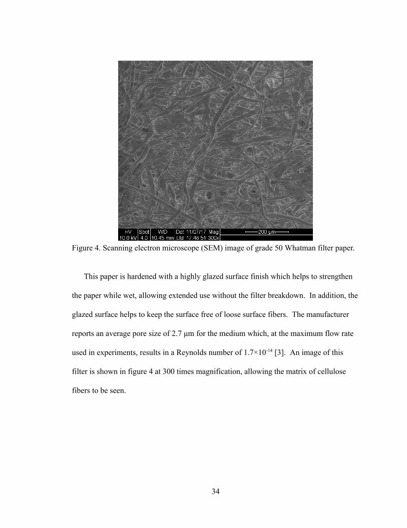
Figure 4. Scanning electron microscope (SEM) image of grade 50 Whatman filter paper.

This paper is hardened with a highly glazed surface finish which helps to strengthen

the paper while wet, allowing extended use without the filter breakdown. In addition, the

glazed surface helps to keep the surface free of loose surface fibers. The manufacturer

reports an average pore size of 2.7 μm for the medium which, at the maximum flow rate

used in experiments, results in a Reynolds number of 1.7×10 ­14 [3]. An image of this

filter is shown in figure 4 at 300 times magnification, allowing the matrix of cellulose

fibers to be seen.

34

The overall rectangular dimensions of the filter paper of 150 mm by 230 mm allow it

to be cut and placed in the 88 mm x 147 mm test area. The thickness of the filter paper is

121 μm, but when wetted swells to approximately 150 μm based on sample testing [3].

4.2 Design of the Hydraulic Resistance Tester

4.2.1 Functional Requirements

To test the application of Darcy’s law in the special case of sheet resistance, a device

was built to direct fluid into a porous medium of a fixed cross section. The device has

one port for fluid flow of a known rate to enter the device and a reservoir for the fluid to

gather and push evenly into the thin porous medium. Along the length of the flow

direction, several ports were placed to test the local pressure in order to track pressure

drop as a function of the distance traveled. Additional pressure ports, transverse to the

flow direction, are included to confirm an even pressure field as the fluid moves through

the porous medium. The device has one exit open atmospheric pressure at the end of the

porous medium, with the same cross sectional area of the porous medium. To test

Darcy’s law, the total volume of fluid into the device must travel to the exit, necessitating

proper sealing at each pressure port and along the outer perimeter of the device. Finally,

a high degree of flatness for the internal surfaces as well as deterministic spacing is

ensured to allow a fixed cross section throughout the device.

35

4.2.2 Kinematic Design and Construction

The design of the Hydraulic Resistance Tester relies on kinematic principles with the

goal to both accurately achieve a known desired cavity thickness in the Z direction and

reliably achieve this thickness with repeated testing trials. In addition, the Hydraulic

Resistance Tester is designed such that feature tolerances in the X­Y directions are not

critical to function, and as a result, the testing apparatus has the fewest tolerance

capability requirements possible for the manufacturing process.

To achieve these design goals, two 6061­T6 aluminum plates were machined from the

flattest available stock material to the design shown in appendix A. The top plate

features a groove along three sides of the perimeter for a rubber gasket, as well as a series

of tapped holes for pressure port readings and another series of tapped holes within the

groove for fastening to the bottom plate and proper sealing. The most critical

dimensional control for both of these plates is the flatness of the primary datum surfaces.

To ensure the highest degree of flatness possible, both plates were lapped on the primary

datum surface. Measurement by a coordinate measurement machine confirmed the

flatness for both plates and will be discussed in greater detail in Section 4.6 below.

The top plate of the Hydraulic Resistance Tester is designed to fit a 0.79 mm thick

nitrile rubber gasket within the machined groove, with additional space along the outer

edge for the displacement of the gasket once compressed. The gasket also includes cut

center holes along its length allowing screws between the top and bottom plates when

36

fastened together. The depth of the groove is chosen such that proper sealing is

accomplished once compressed to the desired thickness of a nominal 315 μm.

To create the desired thickness, polyester spacers are used between the plates.

Originally, particle standards were considered because of their tight diameter tolerance

ensuring a high confidence of cavity thickness within the Hydraulic Resistance Tester.

However, particle standards had many drawbacks such as the potential for Hertz contact

stress from the lime glass particle standards and inconsistent particle placement.

Alternatively, BoPET (polyester) shim stock has a tolerance of approximately 15 μm,

zero risk of contact stress and higher repeatability in placement. After these

considerations, rectangular cut polyester shim stock strips were chosen as the ideal

spacers between the plates. In all experiments they were placed in three areas: two

evenly apart at both sides of the flow exit and one at the back center nearest to the inlet.

This triangular placement ensures repeatability once the Hydraulic Resistance Tester is

assembled and can be seen on the bill of materials in appendix A.

4.3 Fluid Flow Rate Device and Tube Selection

To control liquid volume flow rate into the kinematic device, a syringe pump

(Harvard Apparatus Model 11, Holliston, Massachusetts, USA) is used. This is a low

cost syringe pump with microliter (μL) resolution that operates by a spiral gear,

controlled by high resolution stepper motors which depresses a fixtured syringe. The

syringe diameter is programed into the syringe pump and the internal microprocessor

37

drives the stepper motor to produce the prescribed fluid flow. The syringe pump has a

rated accuracy of ± 0.5% of the displayed flow rate and a “pusher advance” resolution of

0.8 μm travel per motor step.

The typical syringe used has a capacity of 35 mL and the displaced fluid runs through

a sealed polyethylene tube of 1/16th inch (1.59 mm) inner diameter by 1/8th inch (3.18

mm) outer diameter which is the same tubing used throughout the experimental setup

wherever tubing is used for transport fluid. A 10­32 UNF by 1/16th inch (1.59 mm) inner

diameter polypropylene adaptor is used to connect the tubing to the pressure ports of the

kinematic device to create a watertight seal.

38

4.4 Pressure Measurement Methodology

4.4.1 Determining Pressure in Porous Media

The task of selecting the ideal pressure measurement methodology is complicated by

the challenge of initially predicting the expected pressure within the testing device. To

predict pressure, Darcy’s law requires a value of permeability k to be quantified,

dependent on the porous medium. If Forchheimer flow is present, inertial coefficient is

also required which is dependent on the geometry and pathing of the porous medium.

The task of determining media permeability and inertial coefficient is not trivial and is

more often determined experimentally or avoided entirely in other works. As shown in

previous sections, there is little theoretical work available to estimate permeability in

anything other than very idealized media such as packed spheres.

Also challenging is determining what flow regime will be present for a given

experimental setup. Research and theory show that pressure will increase cubically or

quadratically depending on the inertial regime state, leading to very different expected

pressure drops in the porous medium. Research shows there is an inherent difficulty in

predicting this, and most methods often requires observation of the flow before this

determination is made.

4.4.2 Pressure Measurement Selection

Resistance to flow is measured by pressure difference, and common methods for

pressure measurement include manometers and silicon membrane transducers. The

39

selection of manometers for these experiments is driven by the parameters of the

experiment, considerations of off­the­shelf devices, and merits of manometers.

The experimental setup benefits from a pressure device that will allow the air that

initially occupies the porous medium to be completely displaced by the water as it is

pumped into the device. If the chosen pressure measurement device does not allow this,

air would become trapped in the tapped holes and tubes that are connected to the pressure

sensor, potentially exhibiting compressible fluid behavior. In this scenario it is also

uncertain if the pressure sensor is exposed to air, liquid or both, as the testing apparatus is

handled and the trapped air between the testing device and sensor are minimized. Also,

an important parameter is that the experiment would require six pressure measurement

devices making a low cost method more ideal.

To compound these challenges, the parameters of the experiment were not completely

defined at the time of pressure measurement device selection. Before the device is built

the smallest achievable gap in experimentation cannot easily be predicted. Because

Darcy’s law predicts pressure drop is linearly proportional to the gap or thickness, the

difference between the design target of 111 μm and the achieved thickness of 315 μm,

means a pressure change of nearly a factor of three.

Off­the­shelf devices such as silicon membrane transducers do not well support these

experimental parameters. Pressure sensors need to be sourced with a high degree of

certainty on the expected pressure ranges needed. Similarly, the accompanying data

40

acquisition technology requires a high degree of certainty on pressure measurement

resolution. Pressure measurement systems for wet environments with wide ranges, high

accuracy and resolution are commercially available such as omega engineering’s PX209

Series but are cost prohibitive when six sensors are required [76].

However, there are distinct advantages with silicon membrane transducer solutions.

Plate thickness can be optimized to prevent trapped air within device and data acquisition

technology can operate continuously capturing more data and can provide greater insight

into the time dependent behavior of pressure profiles. If approximate pressure ranges can

be predicted or referenced from earlier work, transducer cost can be reduced by choosing

narrower ranges. Finally, if there is little concern for compressible flow behavior, dry air

transducers are ideal because of a greatly reduced cost compared to wet pressure

transducers. The manufacturer Honeywell offers a good selection of such pressure

transducers that fit these functional requirements [77].

A reliable, low­cost method of measuring pressure is to fabricate manometers from

polyurethane tubing and vertical hard plastic tubes to measure water column height

visually. This solution is ideal when internal pressure cannot be easily estimated as the

time to build taller manometers is minimal with little impact to costs. Manometer height

can be adjusted by selection of shorter or longer tubes, depending on the observed

pressures between experiments. For example, a range of column heights between 10 mm

and 1200 mm corresponds to hydrostatic pressure between 980 Pa and 11770 Pa.

41

Because the greatest flow rate is 10 μL/min and the relatively large section of porous

medium flow compared to pores, the inlet pressure losses are negligible and gauge

pressure can be reasonably determined by the recorded manometer height above the plane

of flow [68]. Another benefit of manometers is that air can be completely displaced by

the inlet water removing compressible fluid behavior. Coincidentally, manometers were

used in Darcy’s original experiment [6].

4.5 Experimentation

4.5.1 Experimental Preparation

Before data collection, the device was pre­wetted and tested to ensure even pressure

distribution. This is done by placing manometers on the three pressure ports that run

transverse to the flow direction closest to the inlet and closing all other pressure ports.

Fluid is ran through the device and manometer height is recorded across all three ports

once at steady state to confirm an even pressure distribution in the transverse direction of

flow. This is repeated for the three pressure ports running transverse to flow nearest to

the outlet.

4.5.2 Experimental Conditions

Experimentation is performed with the Hydraulic Resistance Tester set level so

gravitational effects can be ignored. The Hydraulic Resistance Tester is assembled with

two stacked Whatman filter paper samples and the 0.0125 inch (315 μm) polyester shims

around the perimeter. The Hydraulic Resistance Tester is closed with the socket head

42

screws tightened in an alternating star pattern in two rounds of torquing. A torque

screwdriver set to 4 N·m is used to ensure consistent tightening and to prevent over

torque. A 35 mL syringe with distilled water is prepared and then placed in the Harvard

Apparatus model 11 syringe pump. Pneumatic tubes are connected from the syringe to

the Hydraulic Resistance Tester. Pneumatic tubes are also connected to the pressure ports

of the Tester as manometers as seen in the bill of material in appendix A.

Experiments are done at flow rates of 10 μL/min and 5 μL/min. The syringe pump is

set to the appropriate flow rate, the pump is turned on and the time is recorded for the

beginning of the experiment. After 21 to 24 hours, first measurements of the pressures

are taken to ensure a steady state and that capillary effects can be ignored. Although

pressure readings start at different times across experiments, all overlap the 24 to 26 hour

interval to ensure comparable data sets. Some experiments are tracked into the 46 to 48

hour time interval to better understand the transitory behavior of the test setup.

Within intervals of data collection, pressure readings are taken by ruler from the top

surface of the Hydraulic Resistance Tester to the top of each water column’s meniscus in

the manometers. These reading are taken every 15 minutes in approximately a two hour

duration between hour 24 and hour 26.

43

4.6 Sources of Uncertainty

4.6.1 Relative and Combined Error

For this work uncertainty is calculated as a relative error as it contributes to the

calculation of porous media permeability. Permeability k , is defined by Darcy’s law and

shown in equation (51).

(51)

The uncertainty of any given source is applied to equation (51) giving an absolute

uncertainty and then divided by the original k value to give a relative error as a

percentage of k as shown in equation (52). Thus, relative error shows how each source of

uncertainty affects the final uncertainty of k . Also, because not all sources of uncertainty

are symmetric about a center value (such as error due to material compression) or

because a symmetric uncertainty source corresponds to an asymmetric error in k , relative

error is shown as either a positive or negative away from an ideal k value where all inputs

have zero uncertainty.

(52)

The propagation of uncertainty in permeability can be traced through the terms in

equation (51). These factors include the flow accuracy of the pump which is taken from

the product specification previously discussed. Pressure measurements were taken by

observation, thus an uncertainty of ±0.5 mm is assigned to manometer height. This

44

corresponds to a ±5 Pa pressure difference which has a variable impact on the relative

error across experiments. However, calculation shows this relative error has a range of

±0.2% to ±0.5% across all data sets. Fluid viscosity is dependent on ambient temperature

during the experiments and was recorded between 21°C and 22.7°C with an average of

22°C throughout all experiments. These temperatures correspond to an average dynamic

viscosity by table of 0.9544 mPa­s with a tolerance of ±0.2270 mPa·s which in turn

correlate to an uncertainty in k of ±2.38%. Another small contributor are the machining

tolerances of the tapped holes expressed in equation (51) as Δ X . A reasonable positional

tolerance for each hole is ±0.075 mm which when doubled (to account the position of two

holes) correspond to an uncertainty of ±1.09%.

The largest contributors to uncertainty are factors that affect the thickness such as the

material tolerance of the spacer shim. Per the information provided by the distributor

(not available by manufacturer directly) the material tolerance for the shim is ±0.00063

inches (±0.016 mm) which correspond to a +4.8% and ­5.3% uncertainty of k [78]. More

difficult to determine is the compression of the material once in assembly. A reasonable

estimation of compression is approximately 10% of the original thickness which

corresponds to an 11.1% uncertainty of k .

45

Table 1. Summary of uncertainty as relative error for permeability k calculation.

Applying law of propagation of uncertainty, a square root of a sum of squares is used

to combine uncertainties and provide an estimate of total uncertainty [79]. Combined

error u is defined as,

(53)

where f is the function under analysis containing the sources of error, y 1 is the first source

of uncertainty and u 1 is the range of uncertainty of y 1 . The second source of uncertainty

is y 2 and so forth to n uncertainties. When the six sources of uncertainty shown above are

evaluated by equation (53) we yield a combined error of u = 74.5 mm 2 for a 10 μL/min

flow assuming a 2400 Pa, and a u = 74.6 mm 2 for a 5 μL/min flow assuming 1200 Pa.

4.6.2 Unquantified Uncertainty

There are other sources of uncertainty that cannot be quantified as an uncertainty of k

for various reasons. This may be because the uncertainties themselves cannot be easily

quantified, or because the sources have a complex interaction with multiple variables

within equation (53), or possibly because they affect permeability in indirect ways not

46

accounted for by equation (51). An example is the surface roughness of the plates that

were not measured and may have had an effect on the transition of flow regime. This is a

difficult uncertainty to resolve because it was not quantified, there is no method to

correlate the roughness of the boundary condition of closed porous media flow, and

because the mechanisms that affect flow regime are complex.

The width of the flow cross section is an example of a source of uncertainty with a

complex effect on calculated permeability. As stated previously, paper samples were cut

into the sample widths by precision craft knife (X­ACTO #1, Elmer's Products, Inc., High

Point, NC) and a finely graduated ruler. A reasonable estimation for the width tolerance

is a tenth of a millimeter as this is approximately the width of the blade. However, the

tolerance effect is not limited to the sensitivity to equation (51) but there is also the

compounding effect of thin unobstructed flow paths which would have a significant

impact to calculated permeability. It is also difficult to determine if the variation in width

actually translates to creating these channels because the complaint rubber gasket has a

high likelihood of constricting flow through the porous medium. However, there is

reason to believe this type of event is rare as there was only one instance observed with

leakage through the sides. In this single occurrence, zero pressure readings for all

manometers were recorded from a 10 μL/min to 1000 μL/min flow rate.

Another source of uncertainty that cannot be correlated to a known uncertainty of k is

the flatness of the plates. Despite that flatness measurements were taken on both plates

47

by a coordinate measurement machine, it is unclear exactly how these surface topologies

effect calculated permeability. Variations in both plate’s flatness could lead to localized

flow velocities and permeabilities as the distance between plates narrow choking flow

and compressing the porous medium. Obviously, large variations in flatness could lead to

serious doubt over all experimentation as the flow through the porous medium would not

be homogenous in the transverse direction to flow (across the width of the paper). This is

why the transverse pressure was taken at the experiment’s onset to confirm a reasonable

homogeneous flow. The measurements from a Zeiss O­INSPECT 543 coordinate

measurement machine confirm both plate’s flatness within two micrometers at the onset

of experimentation and can be seen in appendix B.

48

5. RESULTS AND DISCUSSION

5.1 Collected Data

5.1.1 Best Data Representation

Data collected are shown in two forms; one as figure 5 which plots pressure for each

individual port over time, and another shown in figure 6 which stacks the pressure

readings of each pressure port at the location the pressure port is away from the inlet.

Figure 5. Data set 5 pressure readings separated by measurement location as a function of time, measured at intervals over a time interval from 22 hours to 26 hours.

Figure 5 of data set 5 is helpful to show the time dependent behavior to confirm the

overall increasing trend of pressure over time. The graph shows that this increase is

constant and roughly linear which is true for nearly all cases. Other graphs shown in

Appendix C show pressure eventually holding constant, but this is rarer. Because of this

observed behavior, some experiment’s data collection was extended into the 48 hour

range of which all suggest that this increase is not constant and may even reverse. What

49

can be said of the data is that the pressure profiles (pressure drop between ports) remains

approximately constant. A possible explanation for this is that over time the part of the

wetted filter paper exposed to air accumulates particles increasing hydraulic resistance.

This could explain a slow increase on all pressure port readings but constant pressure

differences between ports. Although this is an interesting phenomenon that deserves

investigation, this work seeks to isolate or remove the transience from the data to

investigate the steady­state behavior.

Figure 6. Data set 5 pressure readings as a function of distance from inlet to outlet, measured at intervals over a time interval from 22 hours to 26 hours.

Figure 6 collapses data set 5 onto the pressure measurement positions as measured as

the distance from the inlet. Data shown in this way allow visualization of the pressure

profile throughout the porous medium which is ideal to investigate Darcy’s law.

However, analyzing data as shown in figure 6 is not preferred because the transient

behavior of the data prevents a deterministic pressure reading for a port. A solution is to

50

isolate only the pressure readings at the same instance across all data sets. This allows

representative data sets of individual pressures as shown in figure 7. The instance chosen

to isolate is hour 25 (or as close as possible) as this in the middle of observation for all

data sets and therefore establishes behavior before and after, confirming a relatively

stable process. Figure 7 is the representative pressures of data set 5, showing a very

useful form of the data which allows easy comparison of all data and as such will be the

form in which data sets will be discussed.

Figure 7. Data set 5 at hour 24.75 showing individual pressure readings and a curve fitting the data as a function of distance from inlet to outlet.

5.1.2 Linear and Nonlinear Determination

Figure 7 shows a curve that is fitted to data set 5. The fitted curve shown in these

graphs is done by first determining if the data set is linear or nonlinear in nature. For

example, data set 5 is an experiment at the high flow rate (10 μL/min) but another data

set with the same flow rate shows a different behavior as seen in figure 8. Interestingly,

51

even the seemingly linear behavior seen in figure 8 is not entirely linear as the sixth

pressure port has a zero pressure reading that is omitted from graphs. The lowest

pressure measured is approximately 100 Pa, so the sixth pressure port should be

measurable if the data were completely linear.

Figure 8. Data set 2 at hour 25 showing individual pressure readings and a curve fitting the data as a function of distance from inlet to outlet.

To objectively determine if a data set is linear or nonlinear, R 2 values are calculated

for the first four and five pressure readings in each data set. A reasonable criterion for

linearity is a 4­point and 5­point R 2 value greater than 0.98. The reason that a 6­point R 2

value is not considered is because most data sets do not have a pressure reading for the

sixth pressure port. A 4­point R 2 value is useful to see a data set’s deviation from

linearity as nearly all data sets could be considered linear based on the first four pressure

ports. Table 2 shows an overview of all data sets gathered by experimentation with

52

relevant R 2 values calculated and the determination of each data set as “Linear” or

“Nonlinear.”

Table 2. Maximum pressure, linear regression fit values for flow at 10 µL/min and 5

µL/min.

* Not available because local pressure at port 5 exceeded manometer height. ** Only

partially meets “Linear” classification criteria.

5.2 Analysis

5.2.1 Curve Fit Equations

For the nonlinear data sets many curve types were applied and an R 2 value calculated

in the attempt to find the best form that describes the data. In alignment with

Forchheimer's equation, quadratic forms where initially investigated but these fits did not

have a satisfactory R 2 value. Alternatively, logarithmic equations fit these nonlinear data

sets quite well with the form shown in equation (54). Table 3 shows the logarithmic

curve fitted equations and R 2 value for all non­zero pressure values within data sets

classified as nonlinear. In table 3, A is a shape factor, B controls the location of the

53

asymptotic pressure drop, and C represents the maximum pressure within the porous

medium.

(54)

Table 3. Flow rate, coefficients and regression fit values for data sets fitted by equation

(54).

Similarly, we can display the linear curve fit data sets that follow equation (55) with

values shown in table 4. In Table 4, coefficient C has the same meaning as table 3 and

represents the maximum pressure within the porous medium as an arithmetic shift above

the independent axis, and D is the slope of linear pressure drop within the porous

medium.

(55)

54

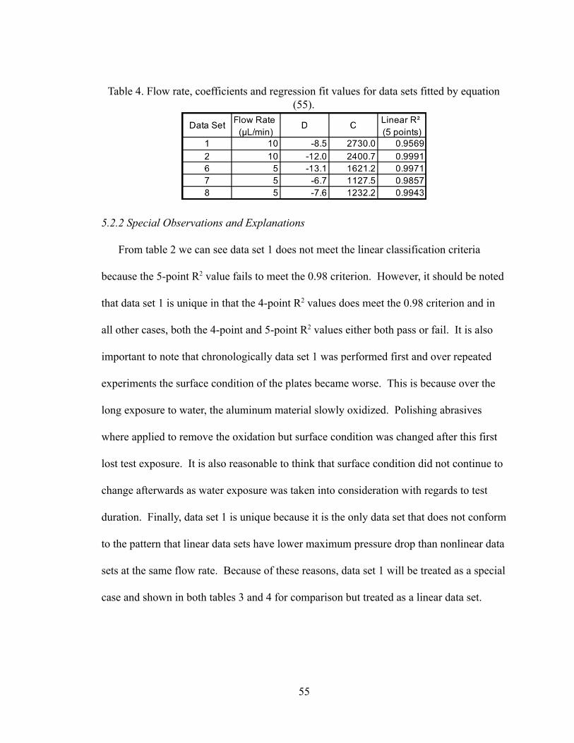
Table 4. Flow rate, coefficients and regression fit values for data sets fitted by equation (55).

5.2.2 Special Observations and Explanations

From table 2 we can see data set 1 does not meet the linear classification criteria

because the 5­point R 2 value fails to meet the 0.98 criterion. However, it should be noted

that data set 1 is unique in that the 4­point R 2 values does meet the 0.98 criterion and in

all other cases, both the 4­point and 5­point R 2 values either both pass or fail. It is also

important to note that chronologically data set 1 was performed first and over repeated

experiments the surface condition of the plates became worse. This is because over the

long exposure to water, the aluminum material slowly oxidized. Polishing abrasives

where applied to remove the oxidation but surface condition was changed after this first

lost test exposure. It is also reasonable to think that surface condition did not continue to

change afterwards as water exposure was taken into consideration with regards to test

duration. Finally, data set 1 is unique because it is the only data set that does not conform

to the pattern that linear data sets have lower maximum pressure drop than nonlinear data

sets at the same flow rate. Because of these reasons, data set 1 will be treated as a special

case and shown in both tables 3 and 4 for comparison but treated as a linear data set.

55

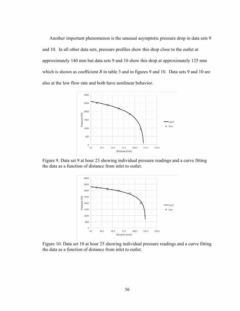
Another important phenomenon is the unusual asymptotic pressure drop in data sets 9

and 10. In all other data sets, pressure profiles show this drop close to the outlet at

approximately 140 mm but data sets 9 and 10 show this drop at approximately 125 mm

which is shown as coefficient B in table 3 and in figures 9 and 10. Data sets 9 and 10 are

also at the low flow rate and both have nonlinear behavior.

Figure 9. Data set 9 at hour 23 showing individual pressure readings and a curve fitting the data as a function of distance from inlet to outlet.

Figure 10. Data set 10 at hour 25 showing individual pressure readings and a curve fitting the data as a function of distance from inlet to outlet.

56

An explanation for this behavior is that this early pressure drop is symptomatic of

porous media flow (under these conditions) in which inertia falls below a critical value.

Acute local pressure drop at approximately 125 mm can also be observed in the linear

data as well despite that initial pressure is much lower for linear profiles. Figure 11

shows this early pressure drop for the linear flow with a low maximum pressure, which

supports the assertion that the early pressure drop is related to viscous forces dominating

over inertial forces. Also, a zero pressure reading does not mean there is zero pressure

but rather the pressure is too low to be detected by the manometer. It is interesting that

data set 10 and data set 6 both show this behavior despite a difference of maximum

pressure by a factor of two. Because of these reasons, it is the recommendation of this

author that this phenomenon be studied further.

Figure 11. Data set 6 at hour 46.50 showing individual pressure readings and a curve fitting the data as a function of distance from inlet to outlet.

57

5.2.3 Calculated Material Properties

According to the accepted theory of porous media flow, material permeability can

only be determined by Darcy (linear) flow because nonlinear flow includes the quadratic

inertial term. The way to visualize this is to plot maximum pressure drop versus flow

rate. For linear data sets maximum pressure drop for 10 μL/min is approximately double

the maximum pressure drop at 5 μL/min as shown in figure 12. This behavior indicates a

consistent material permeability as opposed to nonlinear pressure profiles as shown in

figure 13. Data collection at different flow rates is required to know if nonlinear pressure

profile data sets comply with Forchheimer’s equation.

Figure 12. Maximum recorded pressure drop for linear pressure profile data sets (1, 2, 6, 7 & 8) with an “(H)” or “(L)” to denote high and low flow rate.

58

Figure 13. Maximum recorded pressure drop for linear pressure profile data sets (3, 4, 5, 9 & 10) with an “(H)” or “(L)” to denote high and low flow rate.

Replicate data is required for a strong consensus that these pressure trends hold true.

However, assuming these trends are true we can calculate material permeability as shown

in table 5.

Table 5. Flow rate and calculated material permeability k (mm 2 ) from equation (51) of

linear data sets.

From table 5 we see an average calculated material permeability of 324 mm 2 which has a

standard deviation of 44.6 mm 2 . It is important to note the calculated material

permeabilities have a relatively high agreement considering only five data sets could be

59

used. By dividing fluid viscosity by k , we can show an expression for hydraulic bulk

resistivity (or resistance) based on equation (56). By extension, we can express the

proposed hydraulic sheet resistivity (or resistance) by dividing the hydraulic bulk

resistivity by thickness as shown in equation (30), providing a proposed value for

infinitesimally thin porous media.

(56)

60

6. CONCLUSIONS

6.1 Addressing the Hypothesis

The hypothesis predicts that the lateral fluid flow of a Newtonian incompressible

fluid across thin paper­based porous media in a confined conduit, at Reynolds numbers

much less than one (Re ≪ 1), will be in the Darcy regime. Although some experimental

trials do show Darcy flow, other experimental data contradict this by showing a nonlinear

pressure profile and a nonlinear relationship between maximum pressure and flow rate.

In addition, an expression of hydraulic sheet resistance was derived describing thin sheet

paper­based porous media flow based on electrical sheet resistance. This was shown in

equation (38) which has the same form as electrical sheet resistance shown in equation

(1), except that impetus (as energy per unit mass) decreases linearly instead of

logarithmically because of different flow density field propagation. In addition, the data

do not contradict or preclude the validity of hydraulic sheet resistance.

6.2 Discoveries from Experimentation

It is important to emphasize that there are not enough data to draw any strong

conclusions, but assuming these trends hold true we can make some observations. The

most immediate observation from experimentation is the wide variation in maximum

pressure drop across experiments with fixed conditions. More significant is the discovery

that maximum pressure drop and pressure profile seem to be correlated with low

pressures relating to linear pressure profiles, and high pressures to nonlinear (possibly

61

logarithmic) pressure profiles. Although more data are required to substantiate these

correlations, the implication is that disordered and unconsolidated porous media such as

paper­based porous media, can lead to both Darcy and Forchheimer regime flow with all

other controllable experimental variables held constant. These correlations are likely due

to a wide variance in overall tortuosity of the porous medium. The effect of which can

cause Forchheimer flow (or weak inertia flow) when Reynolds numbers are much less

than one, as in the case of this work where maximum Reynolds number is approximately

1.7×10 ­14 .

6.3 Recommendations for Future Work

6.3.1 Recommendations for Methodology

Different approaches are recommended with regards to experimental setup and

execution. Based on this work, reasonable pressure ranges could be estimated to aid in

the selection of low cost pressure transducer sensors that are usually built for dry

environments. Sensors can be protected against fluid by using polyurethane tubing

between port and sensor, and because there is little time delay in pressure readings

compared to experimental time duration (due to low flow rate), there is little concern with

capturing compressible fluid effects due to the trapped air. Data acquisition technology

can provide more complete data, allowing better isolation of steady state conditions and

better insight into the drivers of transient behavior.

62

In addition, more pressure sensors are recommended to capture pressure profiles. The

acute pressure drop observed near the outlet has the greatest rate of change of nonlinear

profiles and provides the greatest uncertainty in curve fitting. Also recommended is a

pressure sensor as close to the inlet (but within the porous medium) as possible to

determine if maximum theoretical pressure aligns with experimental pressure values.

It is also recommended that testing be done in a clean room or similarly controlled

environment as free particle deposit on the exposed wetted porous media would have an

effect on hydraulic resistance and is a likely contributor to the transient pressure data

observed. It is also recommended for any replicate testing that flow rates are randomized

to help control for possible changing conditions of the equipment.

6.3.2 Recommendations for Testing

To test hydraulic sheet resistance directly, more testing is required with different

aspect ratios. This can be done by changing out gaskets and spacers and applying more

layers of porous media so that the effects of compression are the same. Research

suggests that testing progressively thinner aspect ratios will not support a consistent

calculated hydraulic sheet resistance because wall effects will begin to dominate the

effective hydraulic resistance [67], but for aspect ratios beyond a critical value, the

concept of hydraulic sheet resistance may hold true.

Discoveries found from experimentation prompt other possible future work.

Experimentation affirming the correlation of a maximum low pressure to linear pressure

63

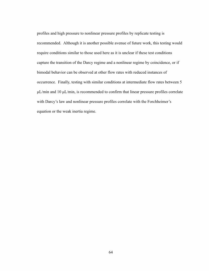
profiles and high pressure to nonlinear pressure profiles by replicate testing is

recommended. Although it is another possible avenue of future work, this testing would

require conditions similar to those used here as it is unclear if these test conditions

capture the transition of the Darcy regime and a nonlinear regime by coincidence, or if

bimodal behavior can be observed at other flow rates with reduced instances of

occurrence. Finally, testing with similar conditions at intermediate flow rates between 5

μL/min and 10 μL/min, is recommended to confirm that linear pressure profiles correlate

with Darcy’s law and nonlinear pressure profiles correlate with the Forchheimer’s

equation or the weak inertia regime.

64

REFERENCES CITED

[1] B. J. Kirby, Micro­ and Nanoscale Fluid Mechanics: Transport in Microfluidic Devices . Cambridge University Press, 2010 [Online]. Available: https://books.google.com/books/about/Micro_and_Nanoscale_Fluid_Mechanics.html?hl=&id=AqsgmAEACAAJ

[2] M. Ahumada, M. Bryning, R. Cromer, M. Hartono, and S. J. Lee, “A thin porous

substrate using bonded particles for reverse­emulsion electrophoretic displays,” in Advances in Display Technologies II , 2012 [Online]. Available: http://dx.doi.org/10.1117/12.909252

[3] "Research & Biopharmaceutical Manufacturing ­ GE Healthcare Life Sciences", GE

Healthcare Life Sciences , 2018. [Online]. Available: https://www.gelifesciences.com/en/us. [Accessed: 07­ Mar­ 2017].

[4] L. R. Volpatti and A. K. Yetisen, “Commercialization of microfluidic devices,”

Trends Biotechnol. , vol. 32, no. 7, pp. 347–350, Jul. 2014 [Online]. Available: http://dx.doi.org/10.1016/j.tibtech.2014.04.010

[5] F. M. Smits, “Measurement of Sheet Resistivities with the Four­Point Probe,” Bell

System Technical Journal , vol. 37, no. 3, pp. 711–718, 1958 [Online]. Available: http://dx.doi.org/10.1002/j.1538­7305.1958.tb03883.x

[6] H. P. G. Darcy, Les Fontaines publiques de la ville de Dijon. Exposition et

application des principes à suivre et des formules à employer dans les questions de distribution d’eau, etc . 1856 [Online]. Available: https://market.android.com/details?id=book­cZRWAAAAcAAJ

[7] M. K. Hubbert and M. King Hubbert, “Darcy’s Law and The Field Equations of The

Flow of Underground Fluids,” Bull. Int. Assoc. Sci. Hydrol. , vol. 2, no. 1, pp. 23–59, 1957 [Online]. Available: http://dx.doi.org/10.1080/02626665709493062

[8] J. R. Philip, “Flow in porous media,” in Theoretical and Applied Mechanics , 1973,

pp. 279–294 [Online]. Available: http://dx.doi.org/10.1007/978­3­642­65590­6_18 [9] F. Wenner, “A method of measuring earth resistivity,” Bulletin of the Bureau of

Standards , vol. 12, no. 4, p. 469, 1916 [Online]. Available: http://dx.doi.org/10.6028/bulletin.282

65

[10]L. Valdes, “Resistivity Measurements on Germanium for Transistors,” Proceedings of the IRE , vol. 42, no. 2, pp. 420–427, 1954 [Online]. Available: http://dx.doi.org/10.1109/jrproc.1954.274680

[11] A. Uhlir, “The Potentials of Infinite Systems of Sources and Numerical Solutions of

Problems in Semiconductor Engineering,” Bell System Technical Journal , vol. 34, no. 1, pp. 105–128, 1955 [Online]. Available: http://dx.doi.org/10.1002/j.1538­7305.1955.tb03765.x

[12] I. Miccoli, F. Edler, H. Pfnür, and C. Tegenkamp, “The 100th anniversary of the

four­point probe technique: the role of probe geometries in isotropic and anisotropic systems,” J. Phys. Condens. Matter , vol. 27, no. 22, p. 223201, Jun. 2015 [Online]. Available: http://dx.doi.org/10.1088/0953­8984/27/22/223201

[13]W. Sobieski, A. Trykozko, “Darcy’s and Forchheimer’s Laws in Practice. Part 1. The

Experiment.” Technical Sciences , vol. 17, no. 4, pp. 321­335, Nov. 2014. [14] J. Bear, “Dynamics of Fluids in Porous Media,” Soil Sci. , vol. 120, no. 2, pp.

162–163, 1975 [Online]. Available: http://dx.doi.org/10.1097/00010694­197508000­00022

[15]R. E. Chapman, Geology and Water: An introduction to fluid mechanics for

geologists . Springer Science & Business Media, 2012 [Online]. Available: https://market.android.com/details?id=book­jvvwCAAAQBAJ

[16] S. M. Hassanizadeh and W. Gray, “High velocity flow in porous media,” Transp.

Porous Media , vol. 2, no. 6, 1987 [Online]. Available: http://dx.doi.org/10.1007/bf00192152

[17]O . O. Alabi, “Validity of Darcy’s Law in Laminar Regime,” Electron. Journal of

Geotech. Eng , vol. 16, 2011 . [18] J. Sawicki, W. Szpakowski, K. Weinerowska, E. Woloszyn, and P. Zima ,

“ Laboratorium Z Mechaniki Płynów I Hydrauliki ,” Technical University of Gdańsk . Gdańsk Poland , 2011 .

[19]K. G. Allen, T. W. von Backström, and D. G. Kröger, “Packed bed pressure drop

dependence on particle shape, size distribution, packing arrangement and roughness,” Powder Technol. , vol. 246, pp. 590–600, 2013 [Online]. Available: http://dx.doi.org/10.1016/j.powtec.2013.06.02

66

[20] F.­Y. Tian et al. , “Pressure drop in a packed bed with sintered ore particles as applied to sinter coolers with a novel vertically arranged design for waste heat recovery,” Journal of Zhejiang University­SCIENCE A , vol. 17, no. 2, pp. 89–100, 2016 [Online]. Available: http://dx.doi.org/10.1631/jzus.a1500088

[21]R. M. Fand, B. Y. K. Kim, A. C. C. Lam, and R. T. Phan, “Resistance to the Flow of

Fluids Through Simple and Complex Porous Media Whose Matrices Are Composed of Randomly Packed Spheres,” J. Fluids Eng. , vol. 109, no. 3, p. 268, 1987 [Online]. Available: http://dx.doi.org/10.1115/1.3242658

[22]L. Weber, D. Ingram, S. Guardia, A. Athanasiou­Ioannou, and A. Mortensen, “Fluid

flow through replicated microcellular materials in the Darcy­Forchheimer regime,” Acta Mater. , vol. 126, pp. 280–293, 2017 [Online]. Available: http://dx.doi.org/10.1016/j.actamat.2016.12.067

[23]D. Seguin, A. Montillet, and J. Comiti, “Experimental characterisation of flow

regimes in various porous media—I: Limit of laminar flow regime,” Chem. Eng. Sci. , vol. 53, no. 21, pp. 3751–3761, 1998 [Online]. Available: http://dx.doi.org/10.1016/s0009­2509(98)00175­4

[24]A. Dybbs and R. V. Edwards, “A New Look at Porous Media Fluid Mechanics —

Darcy to Turbulent,” in Fundamentals of Transport Phenomena in Porous Media , 1984, pp. 199–256 [Online]. Available: http://dx.doi.org/10.1007/978­94­009­6175­3_4

[25]E. Skjetne and J.­L. Auriault, “High­Velocity Laminar and Turbulent Flow in Porous

Media,” Transp. Porous Media , vol. 36, no. 2, pp. 131–147, Aug. 1999 [Online]. Available: https://doi.org/10.1023/A:1006582211517

[26]D. Takhanov, Forchheimer Model for Non­Darcy Flow in Porous Media and

Fractures . 2011 [Online]. Available: https://books.google.com/books/about/Forchheimer_Model_for_Non_Darcy_Flow_in.html?hl=&id=fxvLjgEACAAJ

[27] Jean Barrère (auteur d’une thèse en Mécanique), Modélisation des écoulements de

Stokes et Navier­Stokes en milieux poreux . 1990 [Online]. Available: https://books.google.com/books/about/Mod%C3%A9lisation_des_%C3%A9coulements_de_Stokes.html?hl=&id=HOvXMgEACAAJ

67

[28]C. C. Mei and J.­L. Auriault, “The effect of weak inertia on flow through a porous medium,” J. Fluid Mech. , vol. 222, no. ­1, p. 647, 1991 [Online]. Available: http://dx.doi.org/10.1017/s0022112091001258

[29] J. C. Wodie, T. Levy, “Correction non lineaire da la loi de darcy,” C R Acad. Sci.

Paris Ser. II , vol. 312, pp. 157­161. 1991. [30]M. Rasoloarijaona, J. L. Auriault, “Nonlinear seepage flow through a rigid porous

medium,” European Journal of Mechanics ­ B/Fluids , vol. 13, no. 2, pp. 177­195, 1994.

[31]E. Skjetne and J. L. Auriault, “New insights on steady, non­linear flow in porous

media,” Eur. J. Mech. B. Fluids , vol. 18, no. 1, pp. 131–145, Jan. 1999 [Online]. Available: http://www.sciencedirect.com/science/article/pii/S0997754699800107

[32] P. Forchheimer, “Wasserbewegung durch boden,” Zeitschrift des Vereines deutscher

Ingenieure , vol. 45, no. 50, pp. 1781­1788, 1901. [33]M. Muskat, “The Flow of Homogeneous Fluids Through Porous Media,” Soil Sci. ,

vol. 46, no. 2, p. 169, 1938 [Online]. Available: http://dx.doi.org/10.1097/00010694­193808000­00008

[34]L. Green, P. Duwez, “Fluid flow through porous metals,” Journal of Applied

Mechanics , vol. 18 pp. 39­45, 1951. [35]D. Cornell and D. L. Katz, “Flow of Gases through Consolidated Porous Media,”

Ind. Eng. Chem. Res. , vol. 45, no. 10, pp. 2145–2152, 1953 [Online]. Available: http://dx.doi.org/10.1021/ie50526a021

[36] J. G. Savins, “NON­NEWTONIAN FLOW THROUGH POROUS MEDIA,” Ind.

Eng. Chem. Res. , vol. 61, no. 10, pp. 18–47, 1969 [Online]. Available: http://dx.doi.org/10.1021/ie50718a005

[37] F. A.L. Dullien, Porous Media: Fluid Transport and Pore Structure . Academic Press,

2012 [Online]. Available: https://market.android.com/details?id=book­pPJCOKfZGPkC

[38]Y. A. Buyevich and V. S. Nustrov, “Nonlinear flow in fractured porous media,”

Transp. Porous Media , vol. 12, no. 1, pp. 1–17, 1993 [Online]. Available: http://dx.doi.org/10.1007/bf00616358

68

[39]A. E. Scheidegger, The Physics of Flow Through Porous Media . 1960 [Online]. Available: https://books.google.com/books/about/The_Physics_of_Flow_Through_Porous_Media.html?hl=&id=du2hnQEACAAJ

[40]G. Chauveteau and C. L. Thirriot, “Régimes d’écoulement en milieu poreux et limite

de la loi de Darcy,” La Houille Blanche , no. 2, pp. 141–148, 1967 [Online]. Available: http://dx.doi.org/10.1051/lhb/1967009

[41]D. E. Wright, “Nonlinear flow through granular media,” J. Hydraul. Div. Proc. Amer.

Soc. Civ. Eng. , vol. 94, no. HY4, p. 851­872, 1968. [42] F. A. L. Dullien and M. I. S. Azzam, “Flow rate­pressure gradient measurements in

periodically nonuniform capillary tubes,” AIChE J. , vol. 19, no. 2, pp. 222–229, 1973 [Online]. Available: http://dx.doi.org/10.1002/aic.690190204

[43] J. Geertsma, “Estimating the Coefficient of Inertial Resistance in Fluid Flow

Through Porous Media,” Society of Petroleum Engineers Journal , vol. 14, no. 05, pp. 445–450, 1974 [Online]. Available: http://dx.doi.org/10.2118/4706­pa

[44]A. Firoozabadi, D. L. Katz, and Others, “An analysis of high­velocity gas flow

through porous media,” J. Pet. Technol. , vol. 31, no. 02, pp. 211–216, 1979 [Online]. Available: https://www.onepetro.org/journal­paper/SPE­6827­PA

[45]M. Tiss and R. D. Evans, “Measurement and correlation of non­Darcy flow

coefficient in consolidated porous media,” J. Pet. Sci. Eng. , vol. 3, no. 1, pp. 19–33, Oct. 1989 [Online]. Available: http://www.sciencedirect.com/science/article/pii/0920410589900302

[46] S. Irmay, “On the theoretical derivation of Darcy and Forchheimer formulas,” Eos

Trans. Amer. Geophys. Union , 1958 [Online]. Available: http://onlinelibrary.wiley.com/doi/10.1029/TR039i004p00702/full

[47]Y. Bachmat, “Basic transport coefficients as aquifer characteristics,” I. A. S. H.

Symposium Hydrology of Fractured Rocks , vol. 1, pp. 63­75, 1965 [Online]. Available: http://unesdoc.unesco.org/images/0006/000668/066862mo.pdf

[48]D. Ruth and H. Ma, “On the derivation of the Forchheimer equation by means of the

averaging theorem,” Transp. Porous Media , vol. 7, no. 3, pp. 255–264, 1992 [Online]. Available: http://dx.doi.org/10.1007/bf01063962

69

[49]T. Giorgi, “Derivation of the Forchheimer Law Via Matched Asymptotic Expansions,” Transp. Porous Media , vol. 29, no. 2, pp. 191–206, Nov. 1997 [Online]. Available: https://doi.org/10.1023/A:1006533931383

[50] S. Liu and J. H. Masliyah, “Non­linear flows in porous media,” J. Non­Newtonian

Fluid Mech. , vol. 86, no. 1–2, pp. 229–252, 1999 [Online]. Available: http://dx.doi.org/10.1016/s0377­0257(98)00210­9

[51]Z. Chen, S. L. Lyons, and G. Qin, “Derivation of the Forchheimer Law via

Homogenization,” Transp. Porous Media , vol. 44, no. 2, pp. 325–335, Aug. 2001 [Online]. Available: https://doi.org/10.1023/A:1010749114251

[52]R. W. Zimmerman, A. Al­Yaarubi, C. C. Pain, and C. A. Grattoni, “Non­linear

regimes of fluid flow in rock fractures,” Int. J. Rock Mech. Min. Sci. , vol. 41, pp. 163–169, May 2004 [Online]. Available: http://www.sciencedirect.com/science/article/pii/S1365160904000838

[53]M. Fourar, G. Radilla, R. Lenormand, and C. Moyne, “On the non­linear behavior of

a laminar single­phase flow through two and three­dimensional porous media,” Adv. Water Resour. , vol. 27, no. 6, pp. 669–677, Jun. 2004 [Online]. Available: http://www.sciencedirect.com/science/article/pii/S030917080400048X

[54] P. Macini, E. Mesini, and R. Viola, “Laboratory measurements of non­Darcy flow

coefficients in natural and artificial unconsolidated porous media,” J. Pet. Sci. Eng. , vol. 3–4, no. 77, pp. 365–374, 2011 [Online]. Available: https://www.infona.pl/resource/bwmeta1.element.elsevier­ea73991a­bb78­348b­8725­dafca50c7496 . [Accessed: 16­Feb­2018]

[55] I. Kececioglu and Y. Jiang, “Flow Through Porous Media of Packed Spheres

Saturated With Water,” J. Fluids Eng. , vol. 116, no. 1, pp. 164–170, Mar. 1994 [Online]. Available: http://fluidsengineering.asmedigitalcollection.asme.org/article.aspx?articleid=1427705 . [Accessed: 15­Jan­2018]

[56] J. L. Lage, B. V. Antohe, and D. A. Nield, “Two Types of Nonlinear Pressure­Drop

Versus Flow­Rate Relation Observed for Saturated Porous Media,” J. Fluids Eng. , vol. 119, no. 3, pp. 700–706, Sep. 1997 [Online]. Available: http://fluidsengineering.asmedigitalcollection.asme.org/article.aspx?articleid=1428487 . [Accessed: 18­Mar­2018]

70

[57]G. Schneebeli, “Experience sur la limite sur la validité de la loi de Darcy et l apparition de turbulence dans un e’ coulement de filtration,” La Houille Blanche , vol. 2 no. 41, 1955.

[58]N. N. Beliashevsky, N. G. Bugai, “Hydraulic structure of porous flow in an

individual pore under nonlinear regime,” presented at Republican Proceedings, Hydromechanics, Ukrainian Academy of Sciences, Kiev, Ukraine, 1974.

[59]A. Z. Barak, “Comments on ‘high velocity flow in porous media’ by Hassanizadeh

and Gray,” Transp. Porous Media , vol. 2, no. 6, pp. 533–535, Dec. 1987 [Online]. Available: https://doi.org/10.1007/BF00192153

[60]M. Panfilov and M. Fourar, “Physical splitting of nonlinear effects in high­velocity

stable flow through porous media,” Adv. Water Resour. , vol. 29, no. 1, pp. 30–41, Jan. 2006 [Online]. Available: http://www.sciencedirect.com/science/article/pii/S0309170805001375

[61]E. M. Minsky, “On the turbulent flow through porous media,” Doklady Acad. Nauk

SSSR, vol. 58, no. 3, pp. 409­412, 1951. [62]A. Houpeurt, “Etude analogique de l'écoulement radial circulaire transitoire des gaz

dans les milieux poreux,” Rev. Inst. Fr. Petr. , vol. 8, no. 4, pp.129­151, 1953. [63]H. Ma and D. W. Ruth, “The microscopic analysis of high forchheimer number flow

in porous media,” Transp. Porous Media , vol. 13, no. 2, pp. 139–160, Nov. 1993 [Online]. Available: https://doi.org/10.1007/BF00654407

[64]R. E. Hayes, A. Afacan, and B. Boulanger, “An equation of motion for an

incompressible Newtonian fluid in a packed bed,” Transp. Porous Media , vol. 18, no. 2, pp. 185–198, Feb. 1995 [Online]. Available: https://doi.org/10.1007/BF01064677

[65]X. Liu, F. Civan, and R. D. Evans, “Correlation of the Non­ Darcy Flow

Coefficient,” J. Cdn. Pet. Tech. , vol. 34, no. 10, pp. 50­54, 1995. [66]L. Roblee, R. M. Baird, and J. W. Tierney, “Radial porosity variations in packed

beds,” AIChE J. , vol. 4, no. 4, pp. 460–464, 1958 [Online]. Available: http://onlinelibrary.wiley.com/doi/10.1002/aic.690040415/full

71

[67]D. Nemec and J. Levec, “Flow through packed bed reactors: 1. Single­phase flow,” Chem. Eng. Sci. , vol. 60, no. 24, pp. 6947–6957, Dec. 2005 [Online]. Available: http://www.sciencedirect.com/science/article/pii/S000925090500549X

[68]C. Naaktgeboren, P. S. Krueger, and J. L. Lage, “Inlet and Outlet Pressure­Drop

Effects on the Determination of Permeability and Form Coefficient of a Porous Medium,” J. Fluids Eng. , vol. 134, no. 5, p. 051209, May 2012 [Online]. Available: http://fluidsengineering.asmedigitalcollection.asme.org/article.aspx?articleid=1440580 . [Accessed: 18­Mar­2018]

[69] J. Songok and M. Toivakka, “Modelling of capillary­driven flow for closed

paper­based microfluidic channels,” J. Micromech. Microeng. , vol. 27, no. 6, p. 065001, Apr. 2017 [Online]. Available: http://iopscience.iop.org/article/10.1088/1361­6439/aa6b40/meta . [Accessed: 18­Mar­2018]

[70]H. Noh and S. T. Phillips, “Metering the Capillary­Driven Flow of Fluids in

Paper­Based Microfluidic Devices,” Anal. Chem. , vol. 82, no. 10, pp. 4181–4187, May 2010 [Online]. Available: https://doi.org/10.1021/ac100431y

[71]H. Noh and S. T. Phillips, “Fluidic timers for time­dependent, point­of­care assays

on paper,” Anal. Chem. , vol. 82, no. 19, pp. 8071–8078, Oct. 2010 [Online]. Available: http://dx.doi.org/10.1021/ac1005537

[72]B. Lutz, T. Liang, E. Fu, S. Ramachandran, P. Kauffman, and P. Yager, “Dissolvable

fluidic time delays for programming multi­step assays in instrument­free paper diagnostics,” Lab Chip , vol. 13, no. 14, pp. 2840–2847, Jul. 2013 [Online]. Available: http://dx.doi.org/10.1039/c3lc50178g

[73] J. Wang, M. R. N. Monton, X. Zhang, C. D. M. Filipe, R. Pelton, and J. D. Brennan,

“Hydrophobic sol–gel channel patterning strategies for paper­based microfluidics,” Lab Chip , vol. 14, no. 4, pp. 691–695, 2014 [Online]. Available: http://dx.doi.org/10.1039/c3lc51313k

[74] I. Jang and S. Song, “Facile and precise flow control for a paper­based microfluidic

device through varying paper permeability,” Lab Chip , vol. 15, no. 16, pp. 3405–3412, Aug. 2015 [Online]. Available: http://dx.doi.org/10.1039/c5lc00465a

72

[75] “ Basic Filtration Concepts and Terms ­ pes­membrane”, Pes­membrane.com , 2018. [Online]. Available: http://pes­membrane.com/basic­filtraction.html. [Accessed: 18­ Sep­ 2017].

[76] “General Purpose Pressure Transducer”, Omega.com , 2018. [Online]. Available:

https://www.omega.com/pptst/PX209_PX219.html. [Accessed: 09­ Nov­ 2017]. [77] “PRESSURE TRANSDUCER | Honeywell”, Measurementsensors.honeywell.com ,

2018. [Online]. Available: https://measurementsensors.honeywell.com/Pages/category.aspx?category=PRODUCTTYPES­PRESSURE. [Accessed: 12­ Nov­ 2017].

[78] “McMaster­Carr”, Mcmaster.com , 2018. [Online]. Available:

https://www.mcmaster.com/#9513k42/=1c11y9z. [Accessed: 15­ Nov­ 2017]. [79] “NIST TN 1297: Appendix A. Law of Propagation of Uncertainty”, NIST , 2018.

[Online]. Available: https://www.nist.gov/pml/nist­tn­1297­appendix­law­propagation­uncertainty. [Accessed: 18­ Jan­ 2018].

73

APPENDIX A: APPARATUS TECHNICAL DOCUMENTS

74

75

76

APPENDIX B: COORDINATE MEASUREMENT MACHINE FLATNESS

77

78

79

APPENDIX C: EXPERIMENTAL RAW DATA CHARTS

Pressure Readings Separated by Location Over Time:

Data set 1 pressure readings separated by measurement location over time.

Data set 2 pressure readings separated by measurement location over time.

Data set 3 pressure readings separated by measurement location over time.

Data set 4 pressure readings separated by measurement location over time.

Data set 5 pressure readings separated by measurement location over time.

Data set 6 pressure readings separated by measurement location over time.

80

Data set 7 pressure readings separated by measurement location over time.

Data set 8 pressure readings separated by measurement location over time.

Data set 9 pressure readings separated by measurement location over time.

Data set 10 pressure readings separated by measurement location over time.

81

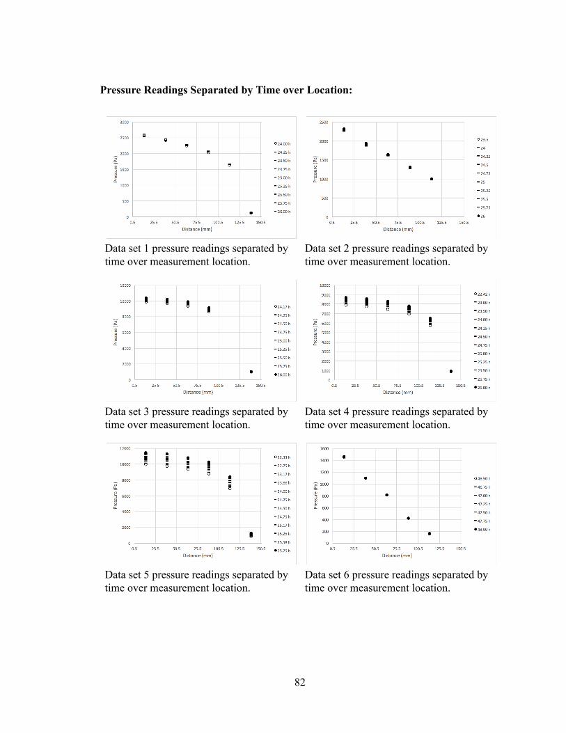
Pressure Readings Separated by Time over Location:

Data set 1 pressure readings separated by time over measurement location.

Data set 2 pressure readings separated by time over measurement location.

Data set 3 pressure readings separated by time over measurement location.

Data set 4 pressure readings separated by time over measurement location.

Data set 5 pressure readings separated by time over measurement location.

Data set 6 pressure readings separated by time over measurement location.

82

Data set 7 pressure readings separated by time over measurement location.

Data set 8 pressure readings separated by time over measurement location.

Data set 9 pressure readings separated by time over measurement location.

Data set 10 pressure readings separated by time over measurement location.

83

Curve Fitted Pressure Readings Over Location at One Instance:

Data set 1 curve fitted pressure readings over location at one instance.

Data set 2 curve fitted pressure readings over location at one instance.

Data set 3 curve fitted pressure readings over location at one instance.

Data set 4 curve fitted pressure readings over location at one instance.

Data set 5 curve fitted pressure readings over location at one instance.

Data set 6 curve fitted pressure readings over location at one instance.

84

Data set 7 curve fitted pressure readings over location at one instance.

Data set 8 curve fitted pressure readings over location at one instance.

Data set 9 curve fitted pressure readings over location at one instance.

Data set 10 curve fitted pressure readings over location at one instance.

85