Embed Size (px)
Citation preview

Univers
ity of
Cape T
own
January 1988
BY MEANS OF AN AIRLIFT RH>
by
R.R. BERG
BSc (Civil Engineering), Cape Town
A thesis subnitted to the University of Cape Town
in partial fulfillment of the requirements for the
degree of Master of Science in Engineering.
Department of Civil Engineering
University of Cape Town
Univers
ity of
Cap
e Tow
n
The copyright of this thesis vests in the author. No quotation from it or information derived from it is to be published without full acknowledgement of the source. The thesis is to be used for private study or non-commercial research purposes only.
Published by the University of Cape Town (UCT) in terms of the non-exclusive license granted to UCT by the author.

Univers
ity of
Cap
e Tow
n
( i)
DEDICATION
To my parents.

Univers
ity of
Cap
e Tow
n
(ii)
DECLARATIOO
I, Rolf Rainer Berg, hereby declare that this thesis is my own work and
that it has not been subnitted for a degree at any other University.
R.R. BERG
January 1988

Univers
ity of
Cap
e Tow
n
(iii)
Airlift ptDDps operating in two-phw:ie gas-liquid flow are investigated with
a view to establishing an analytical technique to aid in theoretically
modelling air-lift pump behaviour.
Extensive work on two test f.!"Cilities constructed at the University of Cape
Town's Hydrotransport Research facility has been done. Various components
needed for the analysis are investigated. 1hese include:
(i)
(ii)
(iii)
(iv)
(v)
static dilation;
dynamic void ratios;
two phase weight component;
two phase friction component;
two phase BL'Celeration component.
Using theoretical models for each canponent and combining these into the
analysis technique, operating characteristics of airlift punps with the
following variables -
(i)
(ii)
(iii)
(iv)
pipe diameters;
gas injection depths;
static lift heights;
suction pipe lengths
have been successfully predicted.

Univers
ity of
Cap
e Tow
n
- i
(iv)
I would like to express thanks to my thesis supervisor, Associate Professor
J.H. Lazarus, for his guidance, enthusiasm and constant interest throughout
the two year thesis period.
Also to Associate Professor F .A. Kilner, the staff of the Department of
Civil Engineering and the Hydrotransport Research Unit team for helpful
discussions and advice during many brainstonning sessions.
I extend thanks to the technical staff, Messrs. G. Bertuzzi, D.J. Botha and
R. F.dge as well as N. Hassen, A. Siko and the rest of the laboratory staff
for their practical aid and assistance during construction and
experimentation stages.
A particular word of thanks to R. Norman and the De Beers Marine staff -
involved in this project for their contributions and support and a special
word of thanks to Mrs P. Jordaan for the typing of this thesis document.
Furthermore I thank the CSIR for financial support throughout the thesis
period.

Univers
ity of
Cape Tow
n
(v)
TABLE OF ~
Chapter
1
2
INTOOOOCTIOO 1.1
LITERATURB AND 'ImrEY
2.1 Introduction 2.1
2.2
2.2
2.4
2.8
2.11
2.11
2.13
2.2
2.3
2.4
2.5
2.6
2.7
Two Jimse flow mechanism
2.2.1 Static conditions
2.2.2 Dynamic coriditions
Two phase gas-liquid flow patterns
Airlift p..mp analysis technique
2.4.1 Static pressure gain
2.4.2 Pressure losses in the suction line
2.4.3 Pressure losses across the gas injector 2.14
2.4.4 Pressure losses in the delivery line 2.16
2.4.4.1 Two phase weight aOO. friction components 2.18
Two }ilase weight models
2.5.1 Introduction
2.5.1.1 Dynanmi.c void ratio
2.5.1.2 Gas-liquid weight equation
2.5.2 Weight model presented by Stenning et al (1968)
2.19
2.19
2.19
2.21
2.22
2.5.3 Weight model presented by Chisholm et al (1983) 2.23
2.5.4 Weight model presented by Giot et al (1986) 2.23
2.5.5 Weight model presented by Clark et al (1985, 1986) 2.24
2.5.6 Weight model presented by Weber et al (1976,1982) 2.24 '
2.5.6.1 Static dilation 2.25
2.5~6.2 Weber et al conversion technique (1976,1982) 2.25
Two phase friction models 2.27
2.6.1 Introduction 2.27
2.6.2 Friction model presented by Stenni.ng et al (1968) 2.27
2.6.3 Friction model presented by Clark et al ( 1986) 2.29 ,, ,. 2.6.4 Friction model presented by Weber et al (1976,1982) 2.29
2.6.5 Friction model presented by Cbi8holm (1983) 2.30
Two 1}ilase acceleration model 2.33

Univers
ity of
Cap
e Tow
n
(vi)
2.8 Conclusion
2.9 Pumping efficiency
3 RESEARCH APPARATUS
3.1 Introduction
3.2 40 um Research apparatus
3.2.1 Overall layout
3.2.2 Suction pipe
3.2.3- Gas injectors
3.2.4 Delivery pipe
3.3 90 nvn Research apparatus
3.3.1 Overall layout
3.3.2 Suet.ion pipe
3.3.3 GaS injectors
3.3.4 Delivery pipe
4 MEASUREMENT TECHNIQUES, CALIBRATION AND ACCURACY .
OF OOLLEC'I'Eo DATA
4.1
4.2
4.3
4.4
4.5
4.6
Introduction
Pressure measurement
4.2.1 Absolute pressure measurement
4.2.2 Differential pressure measurement
4.2.3 Accuracy of pressure measurement
Gas flow rate measurement
4.3.1 Accuracy of gas flow rate measurement
Liquid flow rate measurement
4.4.1 90 nm airlift pump
4.4.2 40 nun airlift pump
4.4.3 Accuracy of liquid flow rate measurement
4.4.3.1 90 nun airlift pump
4.4.3.2 40 mm airlift pump
Static dilation measurement
Dynamic void ratio measurement
4. 6 .1 Accuracy of dynamic void ratio measurement
2.34
2.36
3.1
3.3
3.3
3.3
3.5
3.8
3.10
3.10
3.10
3.10
3.13
4.1
4.1
4.3
4.3
4.5
4.6
4.8
4.9
4.9
4.9
4.11
4.11
4.12
4.12
4.13
4.13

Univers
ity of
Cape T
own
5
6
7
(vii)
EXPERIMENTAL PROCEDURE
5.1 Introduction
5.2
5.3
5.4
5.5
Static dilation tests
40 mm Airlift pump operating tests
5.3.1 Preparation
5.3.2 Operation and varying the lift height
5.3.3 Injection technique comparison
90 um Airlift pump operating tests
5.4.1 Preparation
5.4.2 Operation
5.4.3 Varying the injector aperture
Dynamic void ratio lesls
EXPERIMENTAL RESULTS AND ANALYSIS
6.1 Introduction
6.2 Component results
6.3
6.2.1 Static dilations
6.2.2 Dynamic void ratios
6.2.3 Weight pressure loss
6.2.4 Friction pressure loss
6.2.5 Total pressure loss
Performance curves
6.3.1 General operating curves
6.3.2 40 nm Airlift pump - static lift and
injector depth variation
6.3.3 40 mm Airlift pump - injector technique
comparison
6.3.4 90 nm Airlift pump - injector aperature
variation
6.3.5 Operating curves using lieterature sources
compared with the present analysis
DISCUSSION
7.1 Introduction
7.2. Component Results
7.2.1 Static dilations
5.1
5.2
5.3
5.3
5.4
5.5
5.6
5 .-6 -
5.6
5.7
5.7
6.1
6 .1
6.1
6.2
6.2
6.3
6.3
6.4
6.4
6.4
6.4
6.5
6.5
7.1
7.1
7.1

Univers
ity of
Cap
e Tow
n 8
7.3
(viii)
7.2.2 Dynamic void ratios
7.2.3 Weight pressure loss
7.2.4 Friction pressure loss
7.2.5 Total pressure loss
Airlift pump perfonnance curves
7.3.1 General operating curve
7.3.2 40 11111 Airlift pump - static lift and
injector depth variation
7.3.3 40 nm Airlift pump - injection technique
comparison
7.3.4 90 nm Airlift punp - injector aperature
7.3.5 Operating curve using literature sources
compared with the present analysis
OONCLUSIONS
7.2
7.3
7.4
7.5
7.6
7.6
7.7
7.7
7.7
7.8
8.1
Univers
ity of
Cap
e Tow
n
(ix)
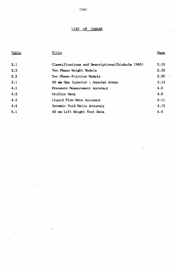
LIST OF TABLES
Table Title ~
2.1 Classifications and Descriptions(Chisholm 1985) 2.10
2.2 Two Phase Weight Models 2.35
2.3 Two Phase Friction Models 2.35 -3.1 90 Rill Gas Injector : Armular Areas 3.13
4.1 Pressure Measurement Accuracy 4.5
·i 4.2 Orifice Data 4.6 ._,.
4.3 Liquid Flow Rate Accuracy 4.11
4.4 Dynamic Void Ratio Accuracy 4.15
5.1 40 nun Lift Height Test Data 5.4

Univers
ity of
Cap
e Tow
n
(x)
LIST OF FIGURES
Figure Title ~
2.1 'l\.io Riase Flow Mechanism 2.3
2.2 Liquid Hold-up 2.6
2.3a Bubble Flow 2.9
2.3b Slug Flow 2.9
2.3c Chum Flow 2.9
2 .• 3d' Annular Flow 2.9
2.4 'l\.io Riase Flow Patterns 2.6
2.5 Airlift Pl.lllp Analysis 2.12
2.6 Friction Factor vs. Reynolds Number Diagram 2.28
2.7 Two Riase Multiplier (Chisholm 1983) 2.32
3.1 40 DID Research Apparatus 3.4
3.2 40 um Airlift Pl.mp Research Apparatus 3.4
3.3 40 DID Gas Injectors 3.6
3.4a Horizontal Injector 3.7
3.4b Vertical Annular Ge.a Injector 3.7
3.5 40 DID Airlift PtlDp Inline, Ball Valve arrl
Pressure Tappings 3.9 3.6a 90 DID Research Apparatus 3.11
3.6b 90 om Airlift Flap Research Apparatus 3.12
3.7 90 nm Gas Injector 3.14 ' ·'
3.8 90 nm Gas Injector 3.15
4.1 Separation Pod 4.2
4.2 Sepe.ration Pod 4.2
4.3 Absolute Pressure Mananeter 4.4
4.4 Differential Pressure Manometer 4.4 4.5 90 om Orifice Arrangement, Pressure Gauge
and Flow Regulating Valve 4.7
4.6 Orifice Plate Arrangement 4.7
4.7 Gas Flow Data Aa..'Ul'SCy 4.8
4.8 90 um Sample Tank Voltme 4.10
4.9 40 DID Bend Meter 4.10
4.10 Ball Valve.Arrangement for Dynamic Void Ratio Tests 4.14

Univers
ity of
Cape T
own
(xi)
6. la Static Dilation 6.6
6. lb Sta tic Dilation 6.6
6.2 Static Dilation Tests 6.7
6.3 Static Dilation Tests 6.7
6.4 40 nm Dynamic Void Ratio Comparisons 6.8
6.5 40 nm Dynamic Void Ratio Comparisons 6.8
6.6 90 nm Dynamic Void Ratio Comparisons 6.9 I
6.7 90 nm Dynamic Void Ratio Comparisons 6.9
6.8 36 nm Pressure Loss Comparison 6 .10
6.9 36 nm Weight Pressure Loss Comparison 6.10
6.10 86 nm Pressure Loss Comparison 6.11
6.11 86 nm Weight Pressure Loss Comparison 6.11
6.12 36 nm Friction Pressure Loss Comparison 6.12
6.13 36 nm Friction Pressure Loss Comparison 6.12
6.14 86 nm Friction Pressure Loss Comparison 6.13
6.15 86 nm Friction Pressure Loss Comparison 6.13
6.16 36 nm Pressure Loss Comparison 6.14
6.17 36 nm Pressure Loss Comparison 6.14
6.18 86 nm Pressure Loss Comparison 6.15 -6.19 86 nm Pressure Loss Comparison 6.15
6.20 36 nm Operating curve 6.16
6.21 36 nun Operating curve 6.16
6.22 86 11111 Operating curve 6.17
6.23 86 nm Operating curve 6.17
6.24 36 nm Lift Comparisons 6.18
6.25 40 nm Injector Type Comparisons 6.18
6.26 90 nm Injector Aperture Variation 6.19
6.27 Comparison with Clark's Data 6.19
6.28 . Comparison with Gibson's Data 6.20
6.29 Comparison with Weber's Data 6.20

Univers
ity of
Cap
e Tow
n
Symbol
A
b
/J c
e.g
E.go
f
g
h = t H
k e K
q
tip
p
Q
R e s
v
w x z p
•
(xii)
NCMENCLATURE
Description
Cross-sectional area
Wetted perimeter
Voltune flow ratio
Empirical coefficient
Armand coefficient
Pipe diameter
Dynamic void ratio
Static dilation
Friction factor
Gravitational acceleration
length
Hydraulic head loss
Entrance coefficient
Constants
Efficiency
Pressure change
Sta tic pressure
Flow rate
Reynolds number
Velocity ratio
Shear stress
Velocity
Liquid superficial velocity
Kinematic viscosity
Weight
Lockhart and Martinelli parameter
Height
Density
Two phase multiplier
m2
m
m
m/s 2
m
m
Pa
Pa
Pa
m/s
m/s
m2 /s
N
m
kg/m,

Univers
ity of
Cap
e Tow
n
Subscripts
F
g
I
t
m
0
Friction
Gas
Inlet
Liquid
Mixture
Standard conditions
(xiii)

Univers
ity of
Cap
e Tow
n
INTRODUCTION 1.1
CHAPI'ER 1
The airlift pump ln lts slmplest form consists of a vertlcal plpe sulxnerged
in a liquid. Air is introduced by means of an air injector near or at the
lower end of this vertlcal plpe. The r lslng alr bubbles cause a dilated
air-liquid mixture· to fonn inside the pipe which is less dense than the
surrounding liquid. Thls pressure imbalance results in the vertical
conveying of the liquid as well as, in required applications, solids up the
inside of the plpe.
This method of hydro-pneumatic transport has been known since the 18th
century. Throughout the 19th century towns and industries were growing
rapidly and airlift pumps were successfully used to satisfy the demand for
water. However, with the developnent of pumps of hlgher efficiencies, the
use of airlift pumps was reduced, with the exception of uses where the
rellability of the pumping operation was more important than lts eff lciency
as well as the conveying of special materials, such as aggressive fluids.
Advantages of the air llft pump are its simple and robust nature. During
operation, breakdowns rarely occur and maintenance of the pumping system is
slmple. These factors render it well suited for deep sea mining a.s well as
the following applications:
shaft and well drilllng
the lifting of fluids containing solids, wastewater and slurries
the dredging of silt
vertical lifting of coal in shafts
- deep sea mlning of manganese modules and diamonds
- cleaning of settling tanks
underwater exploration where pump impellers could damage recovered
material
vertical transport of aggressive and radio-active fluids
the mlxing of fluids and gases in the chemical industry.

Univers
ity of
Cap
e Tow
n
INTOODUCI'ION 1.2
The major disadvantages of the airlift pump are:
( i) a lower efficiency than other pumping methods. In a continuous
pumping operation this could influence power costs considerably. It
is for this reason that the airlift pump is rarely used for the
pumping of water except in cases where sporadic pumping takes place;
( li) a non-continuous flow at the deli very end, caused by pulsating air
slugs.
Although the airlift pump is known for its simplicity of construction and
maintenam ... -e, the theoretical aspects are far from simple. Various
theories based on two phase flow in pipes try to model air lift pump
behaviour. However, because these theories are concerned with specific
airlift pump applications and are partly based on empirical values, it
makes them questionable with respect to general validity.
In Southern Africa the airlift pump is extensively used for the reclamation
of diamond bearing sediments off the west coast in deep water. This
research project has the following objectives:
(a) An investigation into the background and available theories of the
airlift pump.
(b) Design and construct airlift pump models to experimentally investi
gate analytical components and effects of variables on airlift pump
behaviour.
(c) Refinement of two phase flow theory, with the view of establishing a
correlation between theoretical approaches and prototype perfor-
mances.
(d) Optimisation of the design of airlift pumps in general ~e.

Univers
ity of
Cap
e Tow
n
LITERATURE REVIEW & TIIEORY 2.1
CHAPI'ER 2
2.1 Introduction
This review is based on literature obtained from journals and books
dating from 1925 to 1986. Literature has been presented in cotmtries
such as Japan, Russia, Sweden, United Kingdom and West Germany.
Various attempts have been made to analyse airlift pump behaviour
theoretically. · In most of these cases, the theories are concerned
with specific airlift pump designs and thus the design procedures and
methods of analysis vary.
After looking at the mechanism that causes and the various flow
patterns encountered in two phase flow, this literature review
consists of a discussion and analysis of some of the theoretical
methods put forward by authors in an attempt to model airlift pump
behaviour.

Univers
ity of
Cap
e Tow
n
LITERATURE REVIEW &. TmXEY 2.2
2.2 Two phase flow mechanism
Prior to discussing the analysis, it is necessary to understand. how
the air lift pr<X..-ess works.
2.2.1 Static conditions
Figure 2.l(a) shows the layout of a typical airlift punp with
no flow. It L'Onsis ts of a pipe, which ls vertically iDDersed
in a liquid, with its lower end a distance (h 1 + ha) below
the surfac..'e. '!he_ depth to which the pipe is inmersed depends
on the mode of operation of the air lift punp and has an
effect on its pumping characteristics. If, for exwnple, it
were required to pump solid material, the lower en! would
have to be in contact with this solid material.
'Ille other erd of the pipe protrudes a distance h 3 vertically
above the liquid's free surface, which is determined. by the
desired pumping height.
Gas is injected by means of a compressor or blower hose at a
distance h 1 below the surfac..'e, into the vertical pipe. 'lhe
distance ha below the injector point is referred to as the
suction pipe ard the dlst.an<...'e (h 1 + h 3 ) above the injector
point to the delivery outlet, is called the delivery pipe.
'Ille liquid outside the me.in airlift riser is termed the
surrounding column and the lift height is the distance h 3 •
Figure 2. l(a) shows conditions when no gas is injected at the
injector point. The pressure of the surrounding colllllll al
any depth below the liquid surface is in equilibritBD with the
pressure inside the airlift pump. Both the liquids inside and
outside the airlift pump have the same density and the system
is in static equilibrium with no flow taking place.

Univers
ity of
Cap
e Tow
n
NO L
IQUI
D FL
OW
DELI
VERY
OUT
LET
/ DE
UVER
Y PI
PE
h 3
• LI
FT H
EI&H
T
Ah
• DI
LATI
ON
DYNA
MIC
COND
ITIO
NS W
ITH
LIQU
ID F
LOW
LIQ
UID
FLD
NIN&
OUT
~f
n --· -
EXTE
RNAL
UQ
UID
LEV
EL _
_ _
EXTE
RNAL
UQ
UID
LEV
EL -
---t
SURR
DUND
IH&
COW
IN
OF L
illU
m
h t
I &A
S IN
JECT
OR
SUCT
ION
PIPE
h
2
FIGU
RE 2
.1
a
-SL
I&HT
&AS
FLO
W
-IN
CREA
SED
&AS
FLOW
::3~
REPL
ENIS
HED
UQ
UID
FIGU
RE 2
.1 b
FI
GURE
2.1
c
TWO
PHAS
E FL
OW
MEC
HANI
SM
N w

Univers
ity of
Cap
e Tow
n
LITERATURE REVIEW & THEORY 2.4
2 • 2 . 2 PYnami.c Conditions
If gas is allowed to enter the airlift pump at the injector
point, the level of the liquid inside the airlift pipe will
dilate by a distance t\h as shown in Figure 2. l(b). 1his
dilated. distance is maintained until lhe gas input flow is
altered. An increase in the gas flow results in an increased
dilation and a decrease in the gas flow causes a decrease in
the distance t\h. If the gas flow is increased to a point
where t\h is larger than the lift height (h.), the liquid will
flow out of the delivery outlet.
1he liquid which has been discharged at lhe delivery outlet
is replenished at the bottom of the suction line, as shown in
Figure 2.l(c).
A conveying system, whereby the liquid is conveyed vertically
by a distance in excess of the lift height, is established.
1he cause of this is the gas input flow which directly
influences the dilation.
In an attempt to explain the operation of the airlift
prcx...--ess, most authors mention that a gas-liquid mixture of
lesser density than the surrounding coll.mm of liquid f onus
inside the airlift pipe. (Weber 1976, 1982; Clark et al 1986;
Alver 1954; Gibson 1925; Dedegil 1974, 1978, 1986; Giot
1986). Hence, a pressure dis-equilibrium is set up between
the gas-liquid coltllR'l inside lhe air-lift pump, and lhe
surrounding coitDDrl of liquid. To regain equilibrium, the
gas-liquid mixture inside the pipe rises. If the height
required to attain equilibrium is larger than the lift
height, the liquid flows out the top and a dynamic
equilibrium is set up.

Univers
ityof
Cape Tow
n
LITERATURE REVIEW & THIDRY 2.5
'Ib.e components of this dynamic equilibrhm are:
1. Th.e weight of the surrotmdlng column of liquid.
2. Th.e weight of the gas-liquid column inside the
airlift pump.
3. Th.e pressure losses due to the conveying of the
gas-liquid colum. such as friction, isothernal
expansion and entrance effects.
Very few authors actually examine the influence of the gas
bubbles on the dilation. Ha.lde et al 1981, St.enning et al
1968 and Chisholm 1985 however mention this effect in their
analysis.
Consider an airlift tube with no liquid flowing and a single
rising gas bubble, as shown in Figure 2. 2. As soon as the
gas bubble is injected, the liquid level dilates froot point A
to point B. As the bubble rises the liquid 'between the
bubble and the pipe wall flows downwards. Th.e liquid level
remains at point B until the bubble emerges at this point,
whereafter the level drops back down to point A. A
continuous inflow of bubbles at a steady rate would cause the
liquid level to rise to a point C, and remain there, as each
time a bubble emerges at the top it is replaced by another at
the gas injector.
hold-up".
'nlis effect is known as the "liquid
Examining a control vol\.Ulle between points D and E inside the
airlift pipe at any time interval and comparing it to a
control volume at the same depth situated in the surrotmding
column, it is seen that the control volume inside the airlift
pipe consists of a certain percentage gas, causing it to have
a lower density than in the surrounding colt.ml of water. If
there were no dilation and the liquid level inside the pipe
were to remain at point A, then there would be a pressure
dis-equilibrhnn between the two control voltmies. To over
come this, the level inside the airlift pipe rises.

Univers
ity of
Cap
e Tow
n
AIRLIFT TUBE
PREVIOUS LIQUID LEVEL
RISING &AS BUBBLE
DILATED LIQUID LEVEL WITH CONTINOUS BUBBLE INFLOW
DILATED LIQUID LEVEL WITH SINGLE BUBBLE
,--- SURROUNDIN& WATER -Au---- LEVEL
a DOWNWARD FLOWING LIQUID
...... E
FIGURE 2.2 - LIQUID HOLD-UP
BUBBLE FLOW
Cl .... 5 .... ...J
SLU& FLOW
I CHURN FLOW
\__
ANNULAR FLOW
CHARACTERISTIC AIRLIFT PUMP OPERATION CURVE
SAS FLOW
FIGURE 2. 4 - TWO PHASE FLOW PATTERNS
2.6

Univers
ity of
Cap
e Tow
n
LITERAnJRE REVIEW & 'I'H1IDRY 2.7
The operation of the airlift process is thus directly related
to the dilation of the gas-liquid collllUl. This dilation
could be the result of
(a) the "liquid hold-up" effect; and
(b) a density difference between the two control voltunes
inside and outside the airlift pipe.
These two conditions will result in the conveying of liquid
in an airlift pump.

Univers
ity of
Cap
e Town ;
·"
LITERATURE REVIEW & THiroRY 2.8
2.3 Two Phase Gas-Liquid Flow Patterns
'lbere are many flow patterns that can occur in vertical two phase
flow. In the literature a variety of classifications exist in order
to distinguish between these flow patterns. Authors such as Govier
et al and Tai tel et al have produced f onnulas (Chisholm 1983) to
model these classifications; however, because of the large amotmt of
variables encotmtered in two phase flow, these become questionable.
Chisholm (1983) and Clark et al (1986)
classifications for vertical two phase flow.
1. Bubble flow
2. Slug flow
3. Churn flow
4. Annular flow.
present four
'lbese being:
primary
Photographs of these four classifications, taken in the 40 nm airlift
pump test facility at the University of Cape Town, are shown in
Figures 2 • 3 (a) , ( b) , ( c) and ( d) •
Referring to Figure 2.4, bubble flow is defined as very small bubbles
of gas in a continuous liquid phase. 'Ibis flow classification
usually exists at very small gas flow rates and is not often
encountered in operational air lift pumps. Increasing the gas flow
rate results in the formation of slug-flow, which are bullet shaped
slugs of gas known as the "Taylor Bubble" in a continuous liquid
phase. Again this clBBsification occurs at low gas flow rates. As
the gas flow rate is increased, the slug flow changes to churn flow
which is a highly mixed oscillatory flow, and is coumon to all
airlift pumps. At very high gas flow rates the churn flow transforms
into annular flow, where the liquid fo:nns a film around the wall and
the gas is located in a central core.
It is difficult to distinguish visually the point where one flow
classification changes to another. 'Ibis is the reason why so many
other classifications are encotmtered in the literature. Table 2.1
presents some of these classifications which are often encountered
when dealing with vertical two phase gas-liquid flow.

Univers
ity of
Cap
e Tow
n
2.9
FIGURE 2.3a - BUBBLE FLOW FIGURE 2.3b - SLUG FLOW
FIGURE 2.3c - CHURN FLOW FIGURE 2.3d - ANNULP.R FLOW

Univers
ity of
Cap
e Tow
n
Alternative General Alternaiive general classification descriptions Source classification
1 Bubble Froth Hoogendoorn and Buitelar Homogeneous
Stratified bubble } p 1 . b bbl Johnson and Abou-Sabc u satmg u e
2 Plug Elongated bubble Greg Ny , Govier and Intermittent Aziz
Stratified plug Sternling Plug froth Kosterin·
3 Slug Stratified slug Stern ling , Johnson and Abou-Sabe
Splashing flow Kras yak ova Frothy slug Oshinowo and Charles Plug Chierici et al.
4 Churn Froth Oshinowo and Charles Dispersed Kosterin
5 Stratified Divided Kosterin Separated Cresting flow White and Huntington
6 Annular Film Govier and Omer Annular Mist annular Hoogendoorn and Buitela · Ripple flow White and Huntington Slug annular Sternling Wispy annular Collier Ripple flow White and Huntington
TABLE 2.1 - CLASSIFICATIONS AND DESCRIPTIONS (CHISHOLM 1983)
2. 10
2
3
4

Univers
ity of
Cape T
own
LITERA'ruRE REVIEW & THIDRY 2.11
2.4 Airlift Pump Analyais Technique
Most analysis techniques presented. in the literature are based on
balancing pressures. As stated before, an operating airlift PllDP is
in dynamic equilibrium. nia.t is, the pressure at a point near the
entrance of the suction pipe (the static pressure gain Api) located
in the surrounding coltlDll of liquid is in balance with the pressure
losses due to the conveying of the liquid up the inside of the pipe.
The pressure losses due to the t.'Onveying of the liquid are given as:
1. Pressure losses in the suction pipe (Apa)
2. Pressure losses across the gas injector ( Ap.)
3. Pressure losses in the delivery pipe (dp4 )
Once the three pressure drops and the static pressure gain have been
obtained. it is possible to perform a pressure balance, i.e.
Ap, = Apa + Apa + Ap4 (2.1)
2. 4 .1 Static pressure gain
Referring to Figure 2.5, it is neoessary to first obtain Uie
pressure at a point B which is at the same elevation as the
suction inlet of the air lift tube. This is done using
Bern.ouilli's energy equation, i.e.
where PA = at.mosJiieric pressure
zA = 0 ; reference height
VA = 0 P8
= pressure at point B
~ = - (h1 + ha)
= 0
= p 0
w = ~; pressure losses due to f riotion
where p is the liquid densi l:.y
(2.2)

Univers
ity of
Cape T
own
2. 12
Po • ATMOSPHERIC PRESSURE
~I ~ r?: ... t oqO 0
b3 D 000
~o A REFERENCE HEI&HT
z: oO 0 z • 0 a ~o .... .... c
::II
D AP4 CB w
! .... z:
000 w z ~o a
h1 z oqO
~o
ED z: z: a .... a .... .... c .... s c
::II
I w CB w
AP3 z >-::II .... CD
i5 a: D
w ! z: w z .... _,
5 a
h2 ffi AP2
m
c •P1
J~ 8 z • - (bl + h2)
BERNOULLI ENER&Y EQUATION
FIGURE 2. 5 - AIRLIFT PUMP ANALYSIS
Univers
ity of
Cap
e Tow
n
LITERA'ruRE REVIEW &. THOORY
Equation (2.2) can be rewritten a.a
where Ap1 = Ute static pressure gain obtained when
mdving from point A to point B in Ute
surrounding <..."'Olumn of liquid
2.13
(2.3)
This pressure gain 111Ust balance the following pressure
losses.
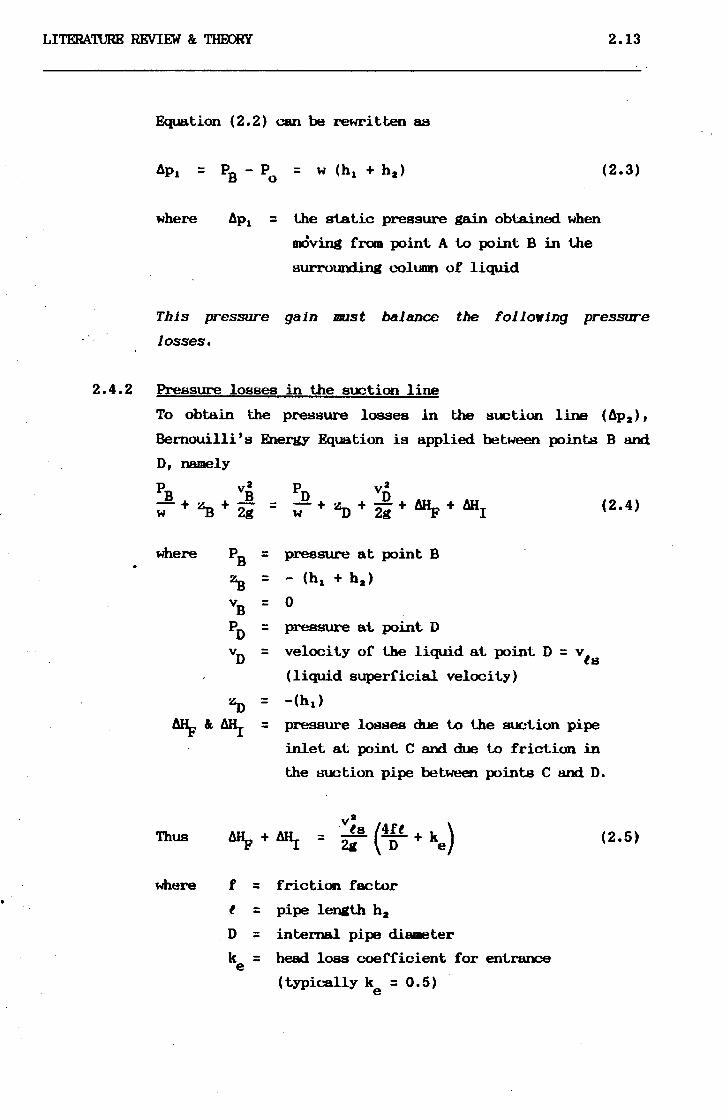
2.4.2 Pressure losses in the suction line
To obtain the pressure losses in the suction line ( Ap2 ) ,
Bernouilli's Energy Equation is applied between points B and
D, namely
PB vB ;;-+~+2g = (2.4)
where PB
~ VB
PD
VD
~
= = = = =
=
pressure at point B
- (h 1 + ha)
0
pressure at point D
velocity of Uie liquid at point D = vta
(liquid superficial velocity)
-(h,)
Al\.- &. ~ = pressure losses due to lhe suction pipe
inlet at point C and due to friction in
the suction plpe between points C and D.
Thus
where f = friction factor
t = pipe lenat:.h ha
D = internal plpe diameter
k = head loss ~-oeff icient for entrance e (typically k = 0.5) e
(2.5)

Univers
ity of
Cap
e Tow
n
LITERATURE REVIEW & THIDRY 2.14
Combining equations (2.4) ard (2.5), the pressure loss in the
suction line can be obtained fran
(2.6)
where Ap2 = the presslll'e loss in the suc..-tion pipe.
2. 4. 3 Pressure losses across the gas iniector
'11>.e gas injector pressure losses a.re obtained by applying the
moment\.lll equation to a control volume between points D and B
on Figure 2. 5. Th.is control volt.me is taken to be very small
ard the gas-liquid weight as well as friction losses are
assumed to be negligible.
'11>.erefore: Prf- + Pn vf,A = PJ!4 + Pg vjt + W + ApiA (Z.7)
where: P 0 = pressure at point D
A = pipe area
Po = density of liquid = pt vD = velocity of the liquid at point D
ApiA = friction of the gas-liquid mixture + 0
W = weight of the gas-liquid mixture + 0
Prf = force at point B, consisting of the pressure
of the liquid as well as the pressure of the
gas acting over their respective areas.
(2.8)

Univers
ity of
Cap
e Tow
n
LITERATURE REVIEW &: nIF.xEY 2.15
It is however assuned that the difference between liquid
pressure Pt and the gas presssure Pg is negligible.
P.B vE A = maoentum force of the gas-liquid mixture,
which can be written as
where
(2.9)
e.g = dynamic void-ratio, whidi is an indication of
the percentage of gas present at that section.
'nlis term will be examined. in Section 2. 5. 1.1.
Pt and Pg = densitie8 of liquid and gas respectively
vt and vg = velocities of liquid and gas respectively.
The velocities of the liquid and gas can be obtained. from
Qt (2.10) Vt = (1 - e.g)A
and vg = l (2.11) e.g A
where Qt = liquid flow-rate
Qg = gas flow rate.
Combining equations ( 2. 7) and ( 2. 9) and. as~ the liquid
and gas pressures are the same after gas injection, the
following equation is obtained. to calculate the pressure drop
(Ap.) across the gas injector:

Univers
ityof
Cape Tow
n
LITERATURE REVIEW & THOORY 2.16
I
At this stage it is important to distinguish between the
velocities vg' vt and vts•
= the · liquid superficial velocity, defined as the
velocity if the liquid were to flow across the whole
pipe section. This quantity relates to the liquid
velocity in the suction pipe, before gas injection.
Qt v. =-A-1:8 -
(2.13)
Velocities vt and vg are velocities after gas injection and
can be obtained from equations (2.10) and (2.11).
2.4.4. Pressure losses in the deliyerx line
To obtain the pressure losses in the delivery pipe, 6p.., the
momenttm equation is again applied to a control volt.me
between points B and F.
Moving up the deli very pipe from points B to F, the pressure
decreases, resulting in the isothermal expmsion of the
bubbles. This effect can be modelled using Boyle's I.aw
gas
Qgo po Qgx = PX (2.14)
where Qgx = gas flow rate at section x in the
delivery pipe.
Qgo = gas flow rate at S.T.P. p = atmospheric pressure.
0 p = pressure at section x. x

Univers
ity of
Cape T
own
LITERATURE REVIEW & 'IHEXllY 2.17
To allow for this effect, it is necessary to analyse the
pressure losses over small increments up the pii)e and then to
integrate over the pipe length. Assuning that the control
volume B to F makes up one such increment, the MomentllD
Equation can be written as:
P"If. + ~ vF!-- = P~ + "F vFA + W + Ap:f' (2.15)
-where
P~ and Py\ = forces at points B and F consisting
of the pressures of liquid and gas
multiplied by their respective areas
as in (2.8)
fl&VHA and ~vFA = manentum forces of the gas-liquid mixture
which can be written as in (2.9-) with its
components as in (2.10) and (2.11).
W = weight of the gas-liquid mixture
Ap~ = friction force of the moving gas-liquid
mixture.
Th.us equation (2.15) can be written as
Ap4 = PB - PF = - [e.g Pg v; + ( 1 - e.g) Pt v; ]B
+ [~g Pg v~ + (1 - E.g) Pt v;]F + W + P/' (2.16)

Univers
ity of
Cap
e Tow
n
2.18
2. 4. 4 .1 Two Jimse ..eight and friction o mpcnenta
To calculate the weight (W) and friction (Aprt) of
the two phase gas-liquid 1Blxture, various lBOdels
have been fJresented in the literature, which will be
examined and modified in further detail •
. .. Firstly, models to calculate the weight component presented.
by Giot et al ( 1986) , Stenning et al ( 1968) , Clark et al
(1986), Chisholm (1983) and We~r (1976, 1982) will be
discussed. '!hereafter friction models presented. by Sterming
et al (1968), Clark (1986), Weber. (1976, 1982) and a two
phase multi plier model presented by Chisholm ( 1983) will be
examined.

Univers
ity of
Cape T
own
'l ..
LITERATURE REVIEW &. THFDRY 2.19
2.5 Two Riase Weight Models
2.5.1 Introduction
In order to calculate the pressure losses in the deli very
line using equations (2.15) or (2.16), one of the components
Uiat has to be evaluated. is the weight of the gas-liquid
mixture.
In the evaluation methods presented. by Chisholm ( 1983) , Clark
et al (1986), Giot et al (1986) and Weber (1976, 1982) use is
made of the dynamic void ratio mentioned in equation ( 2. 9) •
To calculate the weight component, the dynamic void ratio has
to be predicted. and for this reason various methods have been
used in the literature. Stenning et al (1968) suggests a
different method, and does not use dynamic void ratios.
After defining the dynamic void ratio, and presenting the
equation used for calculating the weight of the two phase
gas-liquid mixture, the various void ratio models and the
method presented by Stenning et al will be examined.
2.5.1.1 Dynamic void ratio
A coltlDll of vertically JOOving two Jiiase mixture is
made up of a certain percentage gas and a remaining
percentage of liquid.
'Ille def ini ti on of dynamic void ratio ( 6. g) is the
area of gas divided. by the total area of the pipe
cross-section at any point up the delivery pipe
tmder conditions of mixture flow.
'11lus
(2.17)
where ~ = area occupied. by the gas
A = cross-sectional area of the pipe

Univers
ity
Cape T
own
LITERATURE REVIEW &. THIDRY 2.20
The remaining peI'l...-entage of liquid present can be
obtained from
= Al.
1-E. =g A (2.18)
To calculate the dynamic void ratio, it is necessary
· to determine the fractional areas of the gas and
liquid present at a control section. Thls presents
a certain amount of difficulty because:
1. the gas volume and liquid volume move relative
to each other;
2, the gas voh.une e~ isothermally as the pres
sure decreases up the air-lift pipe length;
3. the gas voltune is influenced by the rate of
movement of the liquid volume;
4. both the gas and liquid volumes present are
influenced by the airlift ptDllp parameters such
as pipe dimension, lift height and suction pipe
depths.
From this it can be seen that in each airlift-pump,
determination of the dynamic void ratio is dependent
on the system characteristics and is a function of:
1. the gas flow
2. the liquid flow \
3. the delivery pipe area
4. the pressure at any section along the delivery
pipe
Univers
ity of
Cap
e Tow
n
LITERAWRE REVIEW&. THEORY 2.22
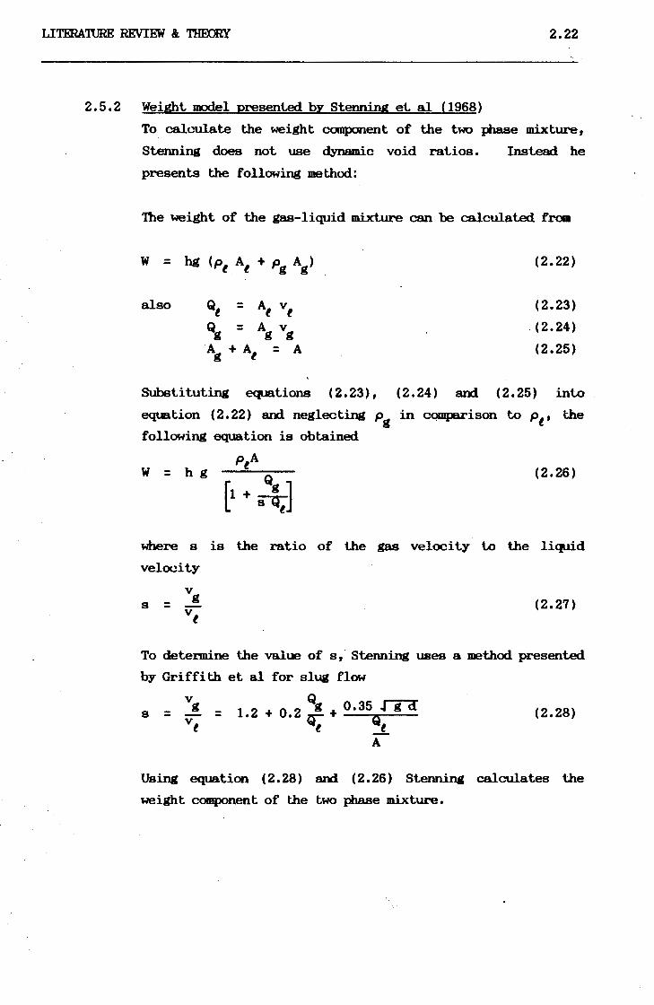
2.5.2 Weight model presented by Stenning et al (1968)
To calculate the weight canponent of the two phase mixture,
Sterming does not use dynamic void ratios. Instead he
presents the following method:
The weight of the gas-liquid mixture can be calculated from
also Qt = At Vt
Qg = Ag vg
Ag + At = A
(2.22)
(2.23)
. ( 2. 24)
(2.25)
Substituting equations (2.23), (2.24) and (2.25) into
equation (2.22) and neglecting Pg in campe.rison to Pt• the
following equation is obtained
ptA w = h g Q
[1 + s SJ (2.26)
where s is the ratio of the gas velocity to tile liquid
velocity
vg s = (2.27)
To detennine the value of s,· Stenning uses a method presented
by Griffith et al for slug flow
vg = 1.2 + 0.2) + 0.35Qm Vt t _1_
s = (2.28)
A
Using equation ( 2. 28) and ( 2. 26) Stenning calculates the
weight component of the two phase mixture.
Univers
ity of
Cap
e Tow
n
\ ~:
LITERA'ruRE REVIEW &. THFXEY 2.23
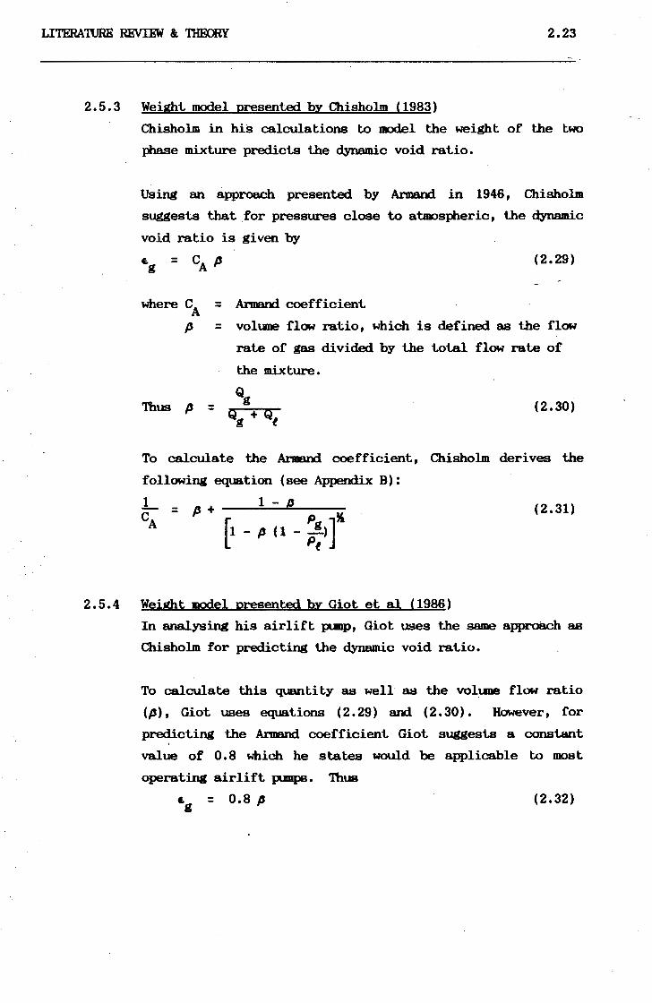
2.5.3 Weight model presented by Chisholm (1983)
2.5.4
Chisholm in his calculations to model the weight of the two
phase mixture predicts the dynamic void ratio.
Using an approach presented by Armand in 1946, Chisholm
suggests that for pressures close to atmosJiieric, the dynamic
void ratio is given by
,._ - c p •g - A
where CA = Armand coeff icienl
(2.29)
p = volune flow ratio, which is defined as the flow
rate of gas divided by the tot.al flow rate of
the mixture.
Thus p (2.30)
To calculate the Armand coefficient, Chisholm derives the
following equation (see Appendix B):
L = p + 1 - /J (2.31) CA [ . Pg]~
1 - p (1 - Pt)
Weight !lOdel presented by Giot et a1 ( 1986)
In analysing his airlift pllllp, Giot uses the same approach as
Chisholm for predicting the dynamic void ratio.
To calculate this quantity as well as the volune flow ratio
(p), Giot uses equations (2.29) and (2.30). However, for
predicting the Armand coefficient Giot suggests a constant
value of 0.8 which he states would be applicable to most
operating airlift pumps. Thus
(2.32)
Univers
ity of
Cap
e Tow
n
LITERATURE REVIEW & THEORY 2.24 .
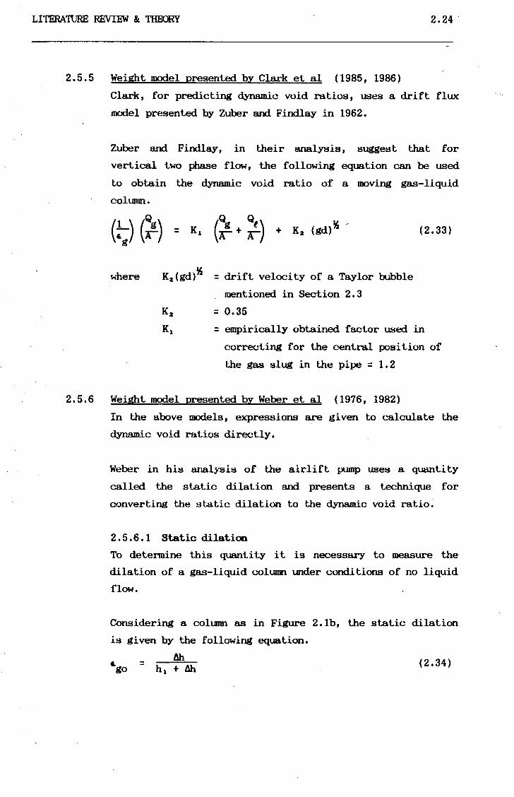
2.5.5 Weight model presented by Clark et al (1985, 1986)
Clark, for predicting dynamic void ratios, uses a drift flux
model presented by Zuber and Findlay in 1962.
Zuber and Findlay, in their analysis, suggest that for
vertical two phase flow, the following equation can be used
to obtain the dynamic void ratio of a moving gas-liquid
ooh.mm.
where K2 (gd)% = drift velocity of a Taylor bubble
mentioned in Section 2.3
K2 = 0.35
(2.33)
K1 = empirically obtained factor used in
correcting for the central position of
the gas slug in the pipe = 1.2
2.5.6 Weight model presented by Weber et al (1976, 1982)
In the above models, expressions are given to calculate the
dynamic void ratios directly.
Weber in his analysis of the airlift pump uses a quantity
called the static dilation and presents a technique for
converting the static dilation to the dynamic void ratio.
2.5.6.1 Static dilation
To determine this quantity it is necessary to measure the
dilation of a gas-liquid column under ~~ndltlons of no liquid
flow.
Considering a cohunn as in Figure 2. lb, the static dilation
ls given by the following equation.
- &i E.go - h 1 + & (2.34)

Univers
ity of
Cap
e Tow
n
LITERATURE REVIEW &. 'IHF.ORY 2.25
Unlike the dynamic void ratio, the static dilation is defined
as the vohme con<...."'elltration of gas enclosed in a column of
liquid and gas during conditions of no mixture flow.
Research by Pichert (1931), Schuring (1934), Bath (1963) and
Weber (1965) has shown that knowledge of the static dilation
has the advantage of being a fW10tion of gas flow and pipe
area only. 'Ibis makes it possible to construct curves for
static dilation which- would be applicable to all pipe sizes.
2.5.6.2 Weber et al oonversim technique (1976, 1982)
Having obtained the static dilation for one particular
delivery pipe size over a range of gas flow rate values,
Weber suggests the following method of converting the static
dilation to the dynamic void ratio.
Under non-flowing conditions, the "mean relative velocity"
between gas and liquid is given by:
v go =
f.go A (2.35)
Assuring that this relative velocity is not affected when
both the liquid and gas flow, then the following equation can
be used to obtain the "mean absolute velocity" of the gas:
v = v + v g go t (2.36)
Also from continuity, . equations ( 2. 10) , ( 2 .11) and ( 2 .18)
apply. Furthermore
f.g = Ag A (2.37)
and .. t =· (1 - f.g) = At A (2.38)

Univers
ity of
Cap
e Tow
n
LITERA'ruRE REVIEW & 'lmXJnT 2.26
Substituting equatioos (2.35), (2.37), (2.38), (2.10), (2.11)
and (2.18) into equation (2.36), the following equation is
obtained for converting the gtatic dilation to the dynamic
void ratio in a vertically moving gas-liquid coll.llm.
The weight of the gas-llquid mixture in the delivery pipe can be
evaluated using one of the above 111entioned models. 7'he applicability
of each of the 'llKXlels presented above will be exaained in further
detail (Refer section 1.2.3).

Univers
ity of
Cape T
own
-
LITERATURE REVIEW&. THIOC)RY 2.27
2.6 n«> PHASE FRICTION K>Dm.s 2.6.1 Introduction
To be able to calculate the pressure loss in the deli very
pipe (Ap4 ) using equation (2.16), the other component that
has to be modelled is the pressure drop due to friction of
the moving two Jiia,se mixture.
In the li teralure, various techniques are presented. 1hese
range from statements such as "the friction pressure loss of
gas-liquid flow is six times that of liquid flow only"
(Gibson, 1925) to complex models using two Jiiase multipliers
(Chisholm, 1983).
Two phase friction models presented by Slenning et al, Clark
et al, Weber et al ard Chisholm, will be examined in further
detail, in order to establish their validity in the airlift
pump analysis.
2.6.2 Friction model presented by Stenning el al (1968)
To calculate the friction in a gas-liquid control column of
length (t), Stenning suggests:
AprA = i: t b
where i: = average wall shear stress
b = wetted perimeter of the pipe = 1f D
t = pipe length = h
(2.40)
to calculate the average wall shear stress ("t'), Sterming uses
an equation presented by Griffith et al:
"t' = f Pt f!t)a(t + Qg) (2.41) t 2 \A ~
where ft = the friction fact.or to be obtained assuning
that the mixture flows as liquid through the
pipe with a volume flow rate of (Qg +Qt),
. (see Figure 2.6).
Canbini.ng equations ( 2. 40) ard ( 2. 41) , Stenning' s friction
pressure model becanes:
(2.42)

Univers
ity of
Cap
e Tow
n
"rj
H
G) c:::: ~
N . "' I "rj
::0
H
(")
t-3
H
0 z "rj >
(")
t-3
0 ::0
<::
.,, (/
) .., :;:;
· ::0
.....
t'1
5·
t-<
: ::
l
z ~
0 t""'
0 .... t::
I 0
(/)
.., z
""""
~ t;:I
t'1
::0
t::
I H
>
G)
::0 ~
0.0
25
I 1
• •
\!~I
,la
min
ar f
low
f =
16
Re
, 0
.02
0.01
8
0.01
6
0.01
4
::
'lam
ina
rfri
tica
l !!:
Tran
sitio
n·
flow
zo
ne •
-zo
ne
'-
! '
I I~~-
'
! I
~ \
--..
' -
l .....
..
I I j
\
I ·~
-r-r-. ""
-I
1:
')'I
(
I"'
J .....
.. ;;- I'
.. -
·1 ; i
~i ~ ~
~ ....
I'
~ I'
r"r--
: Ii
~ }
' ~
r-""
'r c-
---
0.01
2
0.0
1
""' I'
; I
I .\'
/'. ~ R
~ I' ~
. Re.
1
/~
i."
r-r
ITT e
n~~ ~
'
'" ~~-.
........
.....
/ ~ "
I:'
~
I" ~·~
i !
/ ~~
l i
. \
I/
I
0.0
08
0.0
01
.
' ' ' '"
.:\.
I ['-.
" r-
- -I'
--t'--
'r--
~
.....
._,r
-['.
...,_
r-
--I
-.... r--
..
" ~
I 1 i
\
I ~
,...
r-. I"
",..
I•
I
~
L'-.
I I;
! \
' ~ !"
" F::: r"
'r--
; i I
~
~r-
r-P"
~ I 1 I
I
~ r-
""r
N
['-
r-r
I I! j
!'
I i
I ,,, ..;
:~ 1'
.
K
" ...
0.0
06
0.0
05
•rl-R
ivet
ed s
teel
1 -
10 m
m .
r-
i C
on
cret
e 0
.3
-3
mm
0.0
04
I W
ood
stav
e
0.2
-
mm
~
Cas
t ir
on
0
.25
mm
'
Gal
van
ized
ste
el.
15
0 µm
1
Asp
ha 1
.ted
cast
ir
on
120
µm
0
.00
3
_ C
omm
erci
al.
steel.
or
·-45
w
rou
gh
t ir
on
µm
0
.00
2
Dra
wn
tub
ing
1
.5
µm
0.0
02
I
11
J l
I I
I 11
11
I
I I
I I
I
I I I
I l C
ompl
ete
turb
ulen
ce,
roug
h pi
pes
I "
I
' l
I '
' !'
' ' I i
' l'
'r--E3
:::::
I'
r---
j ...
~ --
....
..........
r--
'
r-,....
. '
I ~
''I i'
...... ~~ - -,...,
.. ~ ... -
~
I !'
~ /:::: t-
-..
~r-
I ~ l'
r-~r-r:::
:-~r
--
.. l
jr-~
.___
Sm
ooth
pipes-~ ~
I .....
. .
..... rr
Rey
nold
s nu
mbe
r R
e= u
d 1
I I
I I
1111
i)
·
I
I
I
I
'
.....
r-~I
'" '
-.......
~
.... 0
.00
0,0
01
i"
'r-
~~ "'r
-o .~
ooo,oos·
I°'
r...
.~ r-~
~ ;:
~ ~
I
l(l (l 0 c ( c Cl Ci Cl 0 I
~
1- - ,- .... ,- ·- - ~
;- -,-O
S
04
'
03
.02
.01.
S
.01
00
1
.00
6
00
4
.00
2
.001
0
00
1
.00
06
-00
04
.00
02
.00
01
.ooo
os
.00
00
1
7 9 10
3 2
3 4
56
7
9 104
2 3
4 s
67
9 10
5 2
3 4
.5 6
7
9 2
106
3 4
s 6
7 9 10
7 2
3 4
5 6
7 9 ·1
0•
::0
(!) a <"
(1) 0 c fO
:::r
:J
(t)
(/)
(I)
~
Q:
N
N
CX>

Univers
ity of
Cap
e Tow
n
LITERATURE RE.VIEW & THEORY 2.29
2.6.3 Friction model presented. by Clark et al (1986)
Clark, in his analysis, uses an approach suggested. by
U:xJkhart and Martinelli (1949) in which they state, that the
friction pressure loss is a product of the friction head loss
if liquid alone were flowing in the pipe and a two phase
multiplier f 2 • 'Ihus
(2.43)
where fl = friction factor to be obtained assiming
liquid alone flows through the pipe with a
volume flow rate of Qt • • 2 = two phase multiplier
vts = liquid superficial velocity
D = pipe diameter
To obtain the two phase multiplier f 2, Clark suggests that in
slug flow this quantity can be approximated using:
(2.44)
Substituting equation ( 2. 44) into ( 2. 43) , Clark's friction
pressure loss equation becomes:
2 fl pt h v;s D (1 + 1.5 E.g)
2.6.4 Friction model presented by Weber et al (1976, 1982)
(2.45)
In his airlift pump analysis, Weber uses the following
approach to calculate the friction pressure loss due to the
gas-liquid mixture
2 ft h ( 6pf = D E.g Pg v; + (2.46)
where ft = friction factor to be obtained as in
Section 2.6.2.
E.g = dynamic void ratio
Vt = velocity of liquid
vg = velocity of gas
D = pipe diameter

Univers
ity of
Cap
e Tow
n
LITERATURE REVIEW & THEORY 2.30
2.6.5 Friction model presented by Chisholm (1983)
Chisholm uses a similar approach to Clark, ln stating that
the friction pressure loss is the product of the friction
pressure loss under liquid flow condl tlons and a two phase
multiplier f 2 as in equation (2.43).
However, to calculate the two Jiiage multiplier • 2 , Chisholm
uses the following expression based on work done by LcxJkhart
and MartiJ!elli:
.2 =
where X = the LcxJkhart and Martenelli parameter
c = empirical coefficient.
(2.47)
1he LcxJkhart and Martenelli parameter X is defined as the
square root of the ratio of l:.he friction pressure loss if the
liquid component flows alone to the loss if the gas c...unponent
flows alone.
x2 = (2.48)
from this it can be shown that
ft Pt v; =
f g Pg v~ x2 (2.49)
where ft and fg are calculated using Reynolds m.unbers as
follows:
for ft . Rel =
Vt d . IJ t
(2.50)
for fg Reg = vg d
"'g (2.51)
where IJ t ard IJ g represent the kinematic viscof:d ty of the
liquid and gas respectively.
Univers
ity of
Cap
e Tow
n
LITERA'IURE REVIEW & THOORY 2.31
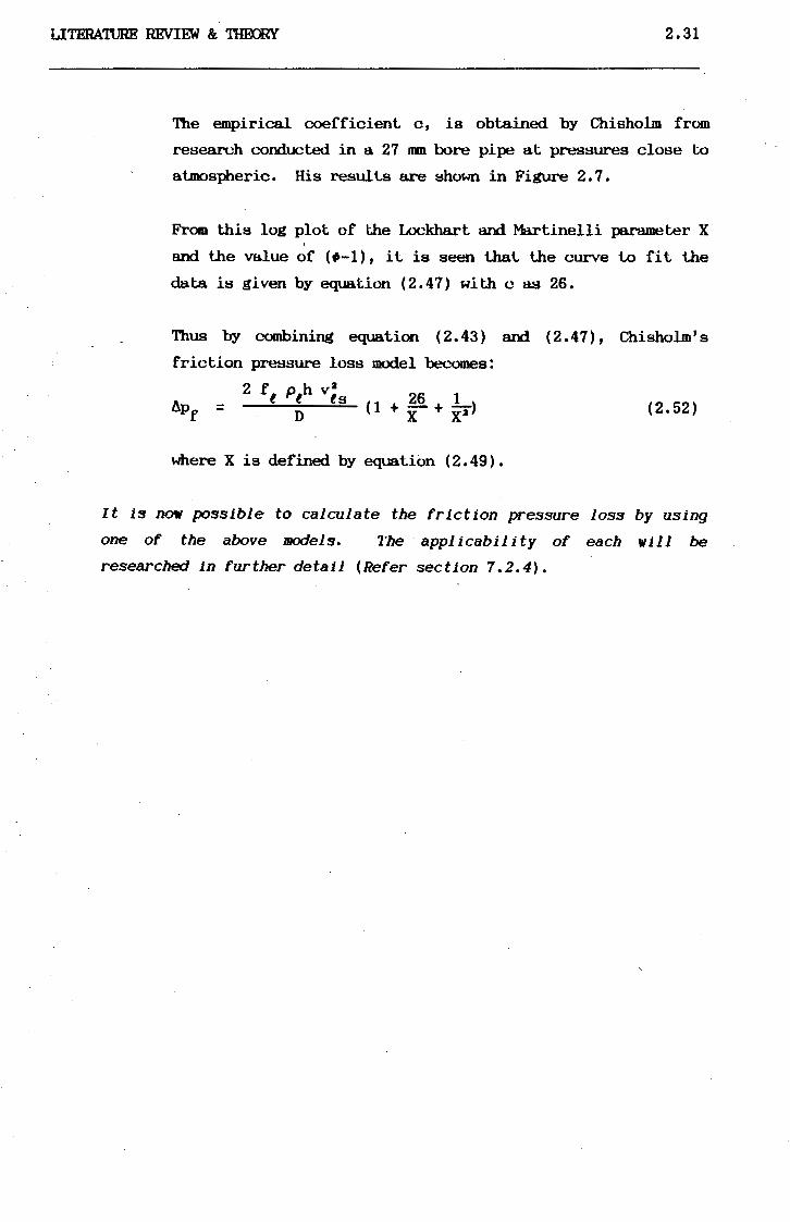
'lbe empirical coefficient c, is obtained by Chisholm from
research conducted in a 27 nm bore pipe at pressures close to
atmospheric. His resul'Ls are shown in Figure 2.7.
From this log plot of the Lockhart and Martinelli parameter X '
and the value of (l>-1), it is seen that the curve lo fit the
data is given by equation (2.47) with c as 26.
'lbus by combining equation (2.43) and (2.47), Chisholm's
friction pressure loss model becomes:
2 f p h Va
fl = t t ts < 1 + 26 + L> Pr D x x2 (2.52)
where X is defined by equation ( 2. 49) •
It is now possible to calculate the friction pressure loss by using
one of the above TllOdels. 1'he applicability of each will be
researched in further detail (Refer section 7.2.4).

Univers
ity of
Cap
e Tow
n
·~ 100Qr-~~~~~~~~~~~~~~~~~~~~~~~~
I ...J
""I!. -e.
' 100
+ 26/X + 11X 2
10
l(
GL
kg/(m2s)
1.0 0 156
e 415 A 581
Q 903 'i1 1269
)( 1987
• 2782
0.1 1.0 100
Lockhart - Martinelli Parameter X
FIGURE 2.7 - TWO PHASE MULTIPLIER (CHISHOLM 1983)
2.32

Univers
ity of
Cap
e Tow
n
..
i ' ,
LITERATURE REVIEW &: THFXlRY 2.33
2.7 Two Phase Acceleration Model
As stated in Section 2. 4. 4, the pressure decreases up the deli very
pipe. 'Ihis decrease results in isothermal expansion of the gas
according to Boyles Law. (equation 2. l<f-) •
Because the llquld flow rema.lns <...-onstant and the area occupled by the
liquid decreases due to the expanding gas, the velocity of the liquid
increases by contlnulty. 'lhls results ln the llquid accelerating up
the delivery pipe causing a pressure drop. 'J
Referring to equatlon (2. Cf ) and (2.1(,), this effect is modelled in
the momentum equation by the tenns:
_ r 6 g pg v ~ + < 1 - E. g > pt v ;] l before
+ r E. g pg v; + < 1 - E. g > pt v ;] l after
(2.53)
In the literature other equations which reduce to equation 2.53 are
presented to model the acceleration effect (Chisholm, 1983).

Univers
ity of
Cap
e Tow
n
LITERATURE REVIEW & THEORY 2.34
2.8 Conclusion
To analyse air lift punps it is necessary ·to calculate pressures
throughout the system. ntese inclt.rle -
1. pressure gain due lo static head;
2. pressure loss in the suction pipe;
3. pressure loss across the air injector; and
4. pressure loss in the deli very pipe.
Pressure losses in the delivery pipe are_ due to -
1. the weight of the two phase mixture;
2. the friction of the two phase mixture with the pipe wall;
3. the acceleration of the two Jiiase mixture caused by the
expending gas bubbles.
Various models exist in the literature lo calc.'lllale the canponent.s of
the delivery pipe pressure losses. Table 2.2 shows models presented
to analyse the weight of Uie gas-liquid mixture and Table 2.3 shows
the models presented to analyse the friction of the gas-liquid
mixtw-e.
Hi;lving calculated all Uie pressures throughout Uie system, it is now
possible to apply a pressure balance using equation (2.1) and to
solve for Uie gas and liquid flow rates in a particular airlift pump.

Univers
ity of
Cap
e Tow
n
2.35 TABLB 2.2 1"'° PHASE WBIGHI' ['l)l)ELS
Author Method Models Equation No.
Stennina et al Direct 1o1ei.ght w = hg ptA
2.6 Q
[1 + ~] v Qll 0.35 pa
(1968) Griffith et al s:..!.: 1.2+0.2cr.+ Q 2.28 Vt t t
A
Qllsholll Dynamic void ratio w = A II h [pll &II + Pt (l-&11) 2 •. 21
(1983) prediction &II =CA p 2.29
using p = Qg
Qll + Qt 2.30
Armend coefficient 1 1 - e. ·- -~
= p +
[ Pg t 2.31
1 - p(l - Pt)
Giot et al Dynamic void ratio w =Allh Cp11 &g + pt(l - &11 )1 2.21
(1986) prediction using & = 0.8 p 2.32 g
Armend coefficient p = Qll
2.30 Qll +Qt
t:lark et al Dynamic void ratio w = A 11 h Cp11 &11 + pt(l - &11
11 2.21
(1986) prediction using (1 )(Qg) (Qg Qt) % E.g A = 1.2 A+ A + 0.36 (gd) 2.33
Zuber and Finlay
h'eber et al Static to dynamic affw = g h [pg E.g + pt(l - E.g)l 2.21
(1976, 1982) void ratio conversion & go 6h
: fn (QllO; A) : h, + Ali 2.34
&II 1 [ t' +Qt) =I 1 +&go Q11
I
J . ,~ + ~ ] - (1+8110( II Qi t)> •_ 4 &110 2.39
'
TABLB 2.3 1"'° FBASB FRICTI~ KlDELS
Author Method Models Equation No.
Stennina et al Griffith Pt (Qt)• ( Q') hnd 6Pf = ft r A 1 + er; A 2.42
(1968)
Cl.ark et al Lockhart and 6pf = 2 ft pth v;s
(1 + 1.5 &11
) 2.45 D (1986) Martinelli
Weber et al 2 ft h
!\pf = -D- (&II P11 v~ + ( 1-&11 ) Pt v; l 2.46
(1976, 1982)
2 f p h v• ~isholm Lockhart and !\pf= t t ts (1 + 26 + 1 ) 2.52 D x i'°
tt Pt v• (1983) Martinelli x• t 2.49 = r, - vr P11 II

Univers
ity of
Cap
e Tow
n
LITERATURE REVIEW & TIIEORY 2.36
2.9 Pumping efficiency
The efficiency of a system is defined as the energy output divided by
the energy input.
q _ energy output - energy input (2.54)
The energy output in the case of airlift pumps operating in two-phase
flow consists of the potential energy gained in raising a volume of
liquid by a tmit height. Referring to figure 2. la, and expressing
the potential energy gain in terms of power~ the output consists of
the power gain in lifting the liquid by a distance (h 1 ) as well as
the power of the liquid jet at the delivery outlet.
(2.55)
where Qe = liquid flow rate
Pe = liquid density
Vt = liquid velocity at the delivery outlet given by
equation ( 2 .IO)
h:a = lift height
The energy input expressed in tenns of power consists of the power
input by the compressor given by
Pi input = Q Po ln-go po
(2.56)
where Qgo = air flow rate
po = atmospheric pressure
Pi = injector pressure
Combining equations (2.54), (2.55) and (2.56) results in the
following equation for calculating the efficiency of an airlift pl.Ullp
operating in two phase flow.
q = (2.57)

Univers
ity of
Cap
e Tow
n
RESEARCH APPARATUS 3.1
CHAPI'ER 3
RESEARCH APPARAnJS
3.1 Introduction
To aid in modelling and analysing airlift pump behaviour, two
research facilities have been constructed in the hydraulics
laboratory of the University of Cape Town. Both systems are airlift
pumps with the following delivery pipe diameters:
1. 40 nnn o.d. and 36 lllll i.d.
2. 90 nm o.d. and 86 nm i.d.
In the operation of an airlift pump the static pressure mentioned in
Section 2.4 is a vital component. To provide this static pressure
both air lift pumps were constructed as recirculating systems with
constant head tanks. Both systems have delivery pipes constructed of
clear P.V.C. in order to observe visually the behaviour of airlift
pumps.
The facilities were designed to investigate the performance of
airlift pumps under the following independent variable conditions:
(a) varying the static lift;
(b) different gas injection techniques;
( c) varying the gas injection depths;
(d) changing apertures of an annular gas injector;
(e) different pipe diameters.
(f) varying the gas flow rate.
Univers
ity of
Cap
e Tow
n
RESEARCH APPARATUS 3.2
During operation, the following dependant variables can be IOOnitored:
(a) pressure losses in the suction line;
(b) pressure losses of the two phase, gas-liquid mixture in the
delivery pipe;
( c) pressure losses across the gas injectors;
(d) static dilations;
( e) dynamic void ratios;
( f) two phase flow patterns.
In this chapter, the two research facilities will be described in
detail, with reference to the three components characteristic to
airlift pumps. These ~ing the suction pipe, the gas injectors and
the delivery pipe.

Univers
ity of
Cap
e Tow
n
RESEARCH APPARATUS
3.2 40 nm Research Apparatus
3.2.1 ~e~!_!~~~
3.3
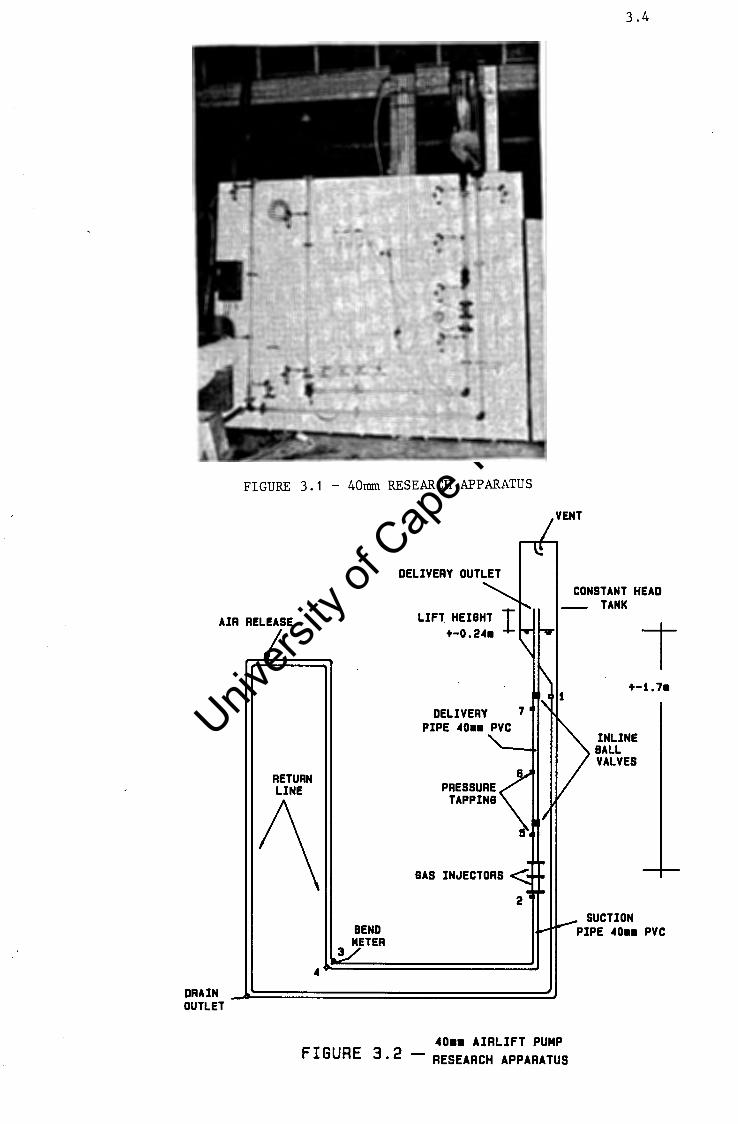
Figure 3.1 shows a Jiiotograph, 8lld Figure 3.2 shows a drawing
of the 40 nm airlift :p.imp researt...il apparatus.
Ref erring to Figure 3. 2, this apparatus is constructed of
40 ~nm o.d., 36 Diil Ld. clear P.v.c. pipe throughout. A
constant head tank is used -
( i) to provide a static pressure at the gas injection
point;
(ii) to alter the lift height;
(iii) to alter the gas injection depth.
The constant head tank is linked directly to the gas injectors via
the suction pipe.
3.2.2 ~!::.1S~!~~-e!~ Referring to Figure 3.2, the suction pipe starts at the base
of the constant head tank arrl ends at the bottaa of the gas
injectors, forming the return line of the recirculating
system. Located along its length are pressure tappings, of
which pressure tapping (1) is used to monitor losses through
the constant heat tank outlet. Pressure tapping (2) provides
the absolute pressure in the system before gas injection and
tappings ( 3) and ( 4) are used to monitor pressures in a bend
meter for liquid flow determination. An air release valve is
provided to facilitate filling and emptying of the apparatus.
Univers
ity of
Cap
e Tow
n
FIGURE 3. 1 - 40mm RESEARCH APPARATUS
DELIVERY OUTLET
3.4
CONSTANT HEAD - TANK
AIR RELEASE r
DRAIN OUTLET
RETURN LINE
BEND METER
3
DELIVERY PIPE '40.. PVC
PRESSURE TAPPIN&
SAS INJECTORS
•O•• AIRLIFT PUMP FIGURE 3. 2 - RESEARCH APPARATUS
+-t. 7•
INLINE BALL VALVES
SUCTION PIPE 40 .. PVC
Univers
ityof
Cape T
own
RESEARCH APPARATUS 3.5
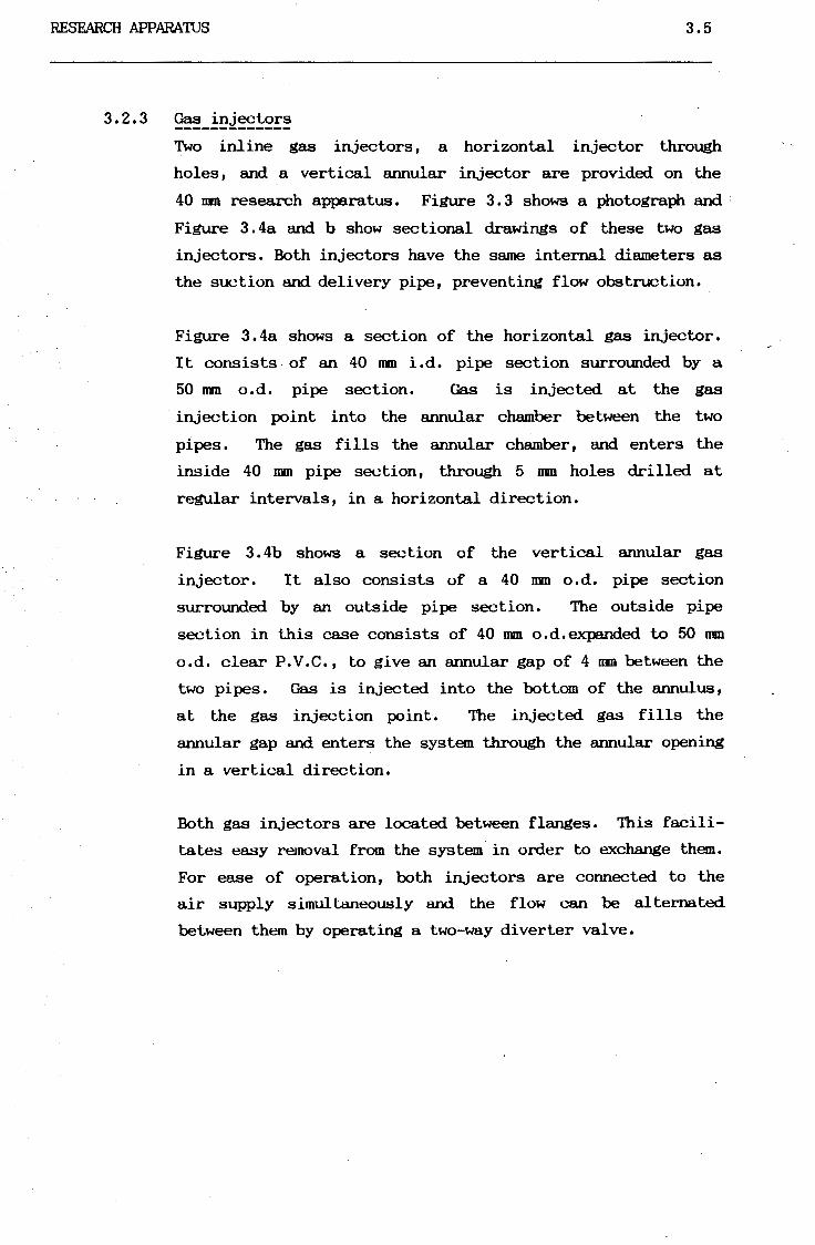
3.2.3 ~-!~J~!:~E~ Two inline gas injectors, a horizontal injector through
holes, and a vertical annular injector are provided on the
40 nm research apparatus. Figure 3. 3 shows a photograph and ,
Figure 3.4a and b show. sectional drawings of these two gas
injectors. Both injectors have the same internal diameters as
the suction and delivery pipe, preventing flow obstruction.
Figure 3. 4a shows a section of the horizontal gas injector.
It consists. of an 40 nun i.d. pipe section surrounded by a
50 nun o.d. pipe section. Gas is injected at the gas
injection point into the annular chamber between the two
pipes. The gas fills the annular chamber, and enters the
inside 40 nm pipe section, through 5 DID holes drilled at
regular intervals, in a horizontal direction.
Figure 3. 4b shows a section of the vertical annular gas
injector. It also consists of a 40 11111 o.d. pipe section
surrounded by an outside pipe section. The outside pipe
section in this case consists of 40 DID o.d.expanded to 50 1IBJ1
o.d. clear P.V.C., to give an annular gap of 4 nm between the
two pipes. Gas is injected into the bottom of the annulus,
at the gas injection point. The injected gas fills the
annular gap and enters the system through the annular opening
ln a vertical direction.
Both gas injectors are located between flanges. This facili
tates easy removal from the system in order to exchange them.
For ease of operation, both injectors are connected to the
air supply simultaneously and the flow can be alternated
between them by operating a two-way diverter valve.

Univers
ity of
Cap
e Tow
n
3.6
. ·.,_ .. ,
.. ,.··
.· .... ·
FIGURE 3.3 - 40rnm GAS INJECTORS

Univers
ity of
Cap
e Tow
n
3.7
f.20
50 Ll8UID-IA8
f 8 off 5H HOLES
&AS IN CTION POIHT
In .. ..
(\I ...
""' BAI - -BAI
ANNULAR CHAMBER
40
L 80 . I FI GU A E 3 . 4 a - HORIZONTAL INJECTOR
f.20 I PVC FLANGE
~~:r---~~~ / 36 /
UllUID-IAI
t A NULAR OPENING
50 ~40m• CLEAR PVC PIPE .-.t.1..._---'=----+1- EXPANDED TO 50mm
in .. .. ~ IAI ··~
ANNULUS
BAS INJECTION POINT
40
t UllUID
I_ 80
FIGURE 3 . 4 b - VERT I CLE ANNULAR GAS INJECTOR
40•• CLEAR PVC PIPE

Univers
ity of
Cap
e Tow
n
RESEARCH APPARAWS 3.8
3.2.4 ~!!~~~~-E!~ Referring to Figure 3. 2, the deli very pipe has a length of
approximately 1. 94 m depending on the preset lift height and
gas injection depth. It starts at the top of the gas
injectors, and ends inside the constant head tank, entering
through its base.
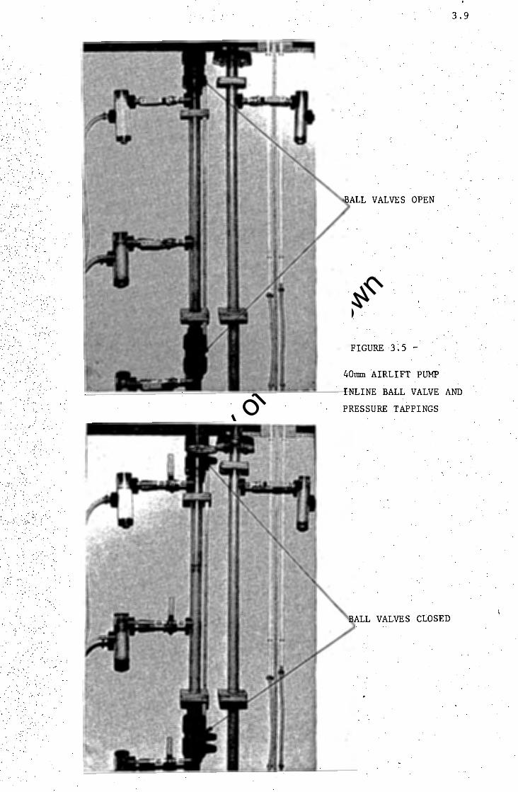
Located along its length are pressure tappings ( 5) , ( 6) and
(7) to monitor pressures in the gas-liquid mixture. These
pressure tappings and two inline.ba.11 :valves are shown in the
photograph on Figure 3.5. The ball valves situated 0.909 m
apart have the same internal diameters as the delivery pipe
and are used to investigate dynamic void ratios.
The deli very outlet is situated in the constant head lank,
which is vented to atmosphere through a 40 um P. V. C. el bow.
Univers
ity of
Cap
e Tow
n
. :' . . . . : .
. .· . ' . ·:·', ..
-... ·
. ·.•·
·- .·-.:
: .·; ., . : .. ·~
:; .. -
.. ;. . . .. >,~:. ,: . :
... ·"·
.. - ·~ .
3.9
BALL VALVES OPEN
FIGURE ·3. 5 -
40rrun AIRLIFT PUMP
INLINE BALL VALVE AND
PRESSURE TAPPINGS
BALL VALVES CtOSED

Univers
ity of
Cap
e Tow
n
RESEARCH APPARATUS 3.10
3.3 90 111n R.esearch Appa.ratus
3.3.1 ~~~!!_!~~~~~
3.3.2
3.3.3
Figure 3. 6a shows a photograph and a diagrammatic layout of
the 90 nm research apparatus. A constant head tank provides
static pressure to a pressure vessel which houses the suction
inlet and ~t of the suction pipe.
At the delivery outlet, flow can be diverted either via a
sample tank for measurement or via a 200 nm return hose back
to the constant head tank, which is approximately 4.5 m above
the gas injector.
~~~!~!LI.>!~ R.eferring to Figure 3 .6 the suction pipe is partly located
inside the pressure vessel to provide a static pressure at
the suction inlet. 470 nm of its length is constructed from
90 nm P. V. C. pipe and the remaining 840 nm is constructed
from 75 nDD N.B. mild steel pipe.
Pressure tapping ( 1) is provided to monitor pressures at the
base of the gas injectors.
~-~~~~~!: The 90 um research apparatus is fitted with a vertical
annular gas injector similar to the one discussed in Section
3. 2. 3. Figure 3. 7 shows a photograph and Figure 3. 8 shows a
section through the gas injector.
It consists of an inner pipe sleeve which can be moved up or
down by means of a hand wheel. This movement in relation to
the outer pipe sleeve causes the annular aperture to vary. I
Gas is injected equally at four points around the ciI'Cum-
f erence of the outer sleeve. The gas fills the annulus which
then enters the delivery pipe through the annular aperture in
a vertical direction.

Univers
ity of
Cap
e Tow
n
3 . 11
Fi gure 3.26 a- 90rnm Resea rch Apparatus

Univers
ity of
Cap
e Tow
n DELIVERY PIPE
90ee PVC
I NL IN! VALVES
"'
7
II
..
3
SAMPLE TANK
PRESSURE TAPPINIB
I
RETURN HOSE
PRE88UR! VESSEL
SUCTION INLET
IOOS!NECIC FLOW OIV!RT!R wlt MICRO SWITCH
----- DELIVERY OUTLET
3. 12
LIFT HElSHT +- II•
200• RETURN HOSE
CONSTANT HEAD TANK
DEPTH +-4.lle
•
90•• AIRLIFT PUMP FIGURE 3. 6 b - RESEARCH APPARATUS

Univers
ityof
Cape T
own
RESEARCH APPARATUS 3.13
Table 3 .1 gl ves the relationship of the m.unbers marked on the
inner pipe sleeve to the annular aperature area.
Marked number Annular gap distance Aperture area ( 11111) (mm2)
0 closed 0 1 1.0 384.1 2 / - 2.5 647.9 3 3.5 918.1 4 4.5 1335.2 5 6.0 1621.1 6 7.0 1766.36 7 8.0 2437.9 8 9.0 2770.9 9 9.5 2939.7
Table 3.1 90 nm gas injector annular areas
3.3.4 ~!~~~~r_E!~
Referring to Figure 3.6, the delivery pipe is attached to the
top of the gas injector and runs vertically for a distance of
approximately 9. 5 m depending on the liquid level in the
constant head tank.
It is constructed of 90 mm o.d., 86 mm i.d. clear P. V .C. pipe. Two inline ball valves, located 1.376 m apart, with
inside diameters the same as the delivery pipe, are used to
monitor the dynamic void ratio in the delivery pipe.
Pressure tappings (2), (3), (4), (5), (6) and (7) are
provided to measure pressures during operation.
The outlet of the delivery pipe leads to a gooseneck flow
diverter which is operated by a pneumatic actuator. A micro
switch is located halfway through the travel of the goose
neck, for time measurement while sampling.

Univers
ity of
Cap
e Tow
n
3. 14
FIGURE 3.7 - 90mrn GAS INJECTOR

Univers
ity of
Cap
e Tow
n
I '
LJIUJD - IAI
FLAN SE--' ..-..&........,
/ OUTER PIPE SLEEVE
BAI IAI
ANNULAR APERTURE 4 off GAS INJECTION
a.---tt5=v7 POINTS
ANNULUS
BLAND SEAL
HANDNHEEL "
FLAN SE
FIGURE 3.8
LJIUJD
INNER PIPE SLEEVE ____/
THREADED COLLAR
/
90•• BAS INJECTOR
3. 15
Univers
ity of
Cap
e Tow
n
MEASUREMENT TECHNIQUF.S, CALIBRATIONS AND ACCURACY OF OOLLECTED DATA
CHAPrER 4
4.1 Introduction
4.1
To analyse the behaviour of airlift pumps, it is necessary to
monitor:
1. pressures,
2. gas flow rates, and
3. liquid flow rates
during operation.
'Ibis chapter discusses the techniques used for the measurement of
these components, as well as measurement of static dllatlons and
dynamic void ratios. Also presented are calibrations and
calculations to determine the accuracy of the collected data.
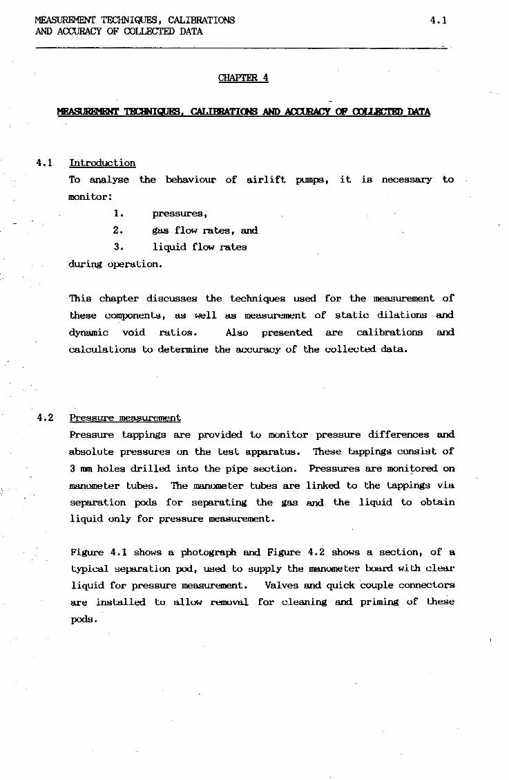
4.2 Pressure measurement
Pressure tappings are provided to monitor pressure differences and
absolute pressures on the test apparatus. These tappings consist of
3 nm holes drilled into the pipe section. Pressures are monitored on
manometer tubes. The manometer tubes are linked to the tappings via
separation pods for separating the gas and the liquid to obtain
liquid only for pressure measurement.
Figure 4. 1 shows a photograph and Figure 4. 2 shows a section, of a
typical separatlon pod, ill:led to supply the manometer board wlth clear
liquid for pressure measurement. Valves and quick couple connectors
are installed to allow removal for cleaning and prlming of these
pods.

Univers
ity of
Cap
e Town
OUTLET TO MANOMETERS
FIGURE 4.1 - SEPARATION POD
INLET FROM PRESSURE TAPPIN&
t!lo ..
40/!10•• CLEAR PVC PIPE
FIGURE 4. 2 - SEPARATION POD
4.2

Univers
ity of
Cape T
own
·,
MEASUREMENT TECHNig,JES, CALIBRATIONS AND ACUJRACY OF COILECTED DATA
4.2.1 ~~!~~~-E~~~-~~~
4.3
Figure 4.3 shows a diagram of the manometer arrangement for
measuring absolute pressures. To prime the manometer, valve
(B) is closed and valves (A) and (C) are opened. Liquid is
used to flush the air through the lllBllOOleter and separation
pods into the pipe. Having flushed all the air out of the
manometer tube and pod, valve (C) is closed and valves (A)
and (B) are opened, for pressure measurement under atmos
pheric conditions.
4.2.2 ~!ff~~~~!~!_E~~~~-~~~~ 'Ihe manometer arrangement for measuring differential pressure
is shown in Figure 4. 4. To prime the manometers, firstly
valve (A) is closed and valve (D) and (B) are opened. Liquid
is used to flush the air through the top pod into the pipe.
Tiien valve (B) is closed and valve (A) opened, now flushing
through the bottom pod. Ha.vi.Ila flushed all the air out the
manometer tubes and pods, valve (D) is closed and valves (A)
and (B) are opened for pressure measurement. To bring the
levels into a readable range, the tops of the menometer tubes
are pressurised by blowing air in through a pressurising
nipple at (C).
All measurements are converted into pressures using:
p = pt g Ah
where pt = the density of the liquid in the manometer
Ah = the actual or differential heights measured on
the manometer tubes
P = pressure
(4.1)

Univers
ity of
Cap
e Tow
n
AIR RELEASE VALVE
B
LIQUID VALVE c
MANOMETER TUBE
I /
PIPE
SEPARATION POD l ISOLATION VALVE AND CONNECTOR
FIGURE 4 3 - ABSOLUTE PRESSURE · MANOMETER
PRESSURIZINB NIPPLE
MANOMETER TUBES
D
I LIQUID VALVE
FIGURE 4.4
A
PIPE
ISOLATION VALVES AND CONNECTORS
~ DIFFERENTIAL PRESSURE MANOMETER
4.4
Univers
ity of
Cap
e Tow
n
r , ' I . : )
'· _;,/
MEASUREMENT TECHNI~, CALIBRATIONS AND ACCURACY OF COLLECTED DATA
4.5
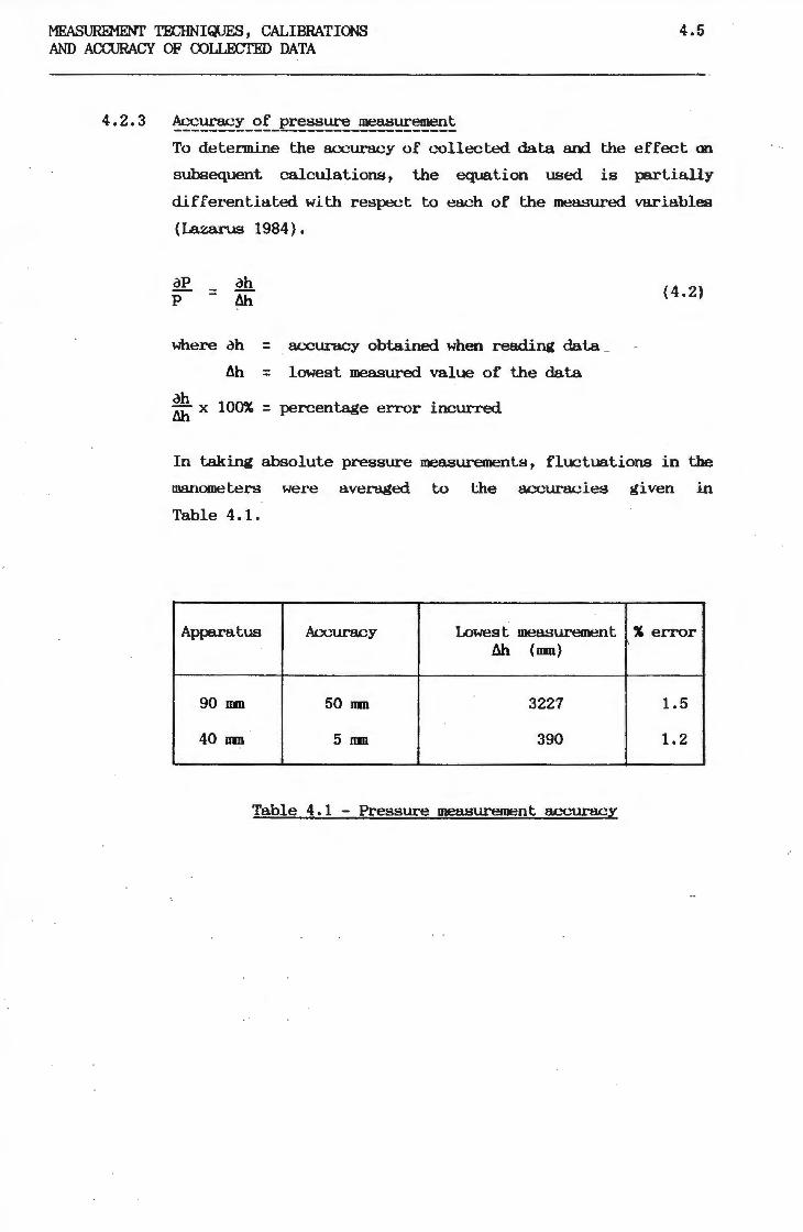
4.2.3 ~~~~-~f _e~~~~~-~~~~~!: To determine the accuracy of collected data and the effect on
subsequent calculations, the equation used is partially
clif ferentlated wlth respect to each of the measured variables
(Lazarus 1984 ) .
where ah = accuracy obtained when reading data _
db = lowest measured value of the data
ah - x 100% = percentage error incurred db
(4.2)
In taking absolute pressure measurements, fluctuations in the
lllBllometers were averaged to the accuracies ~iven ln
Table 4.1.
Apparatus Accuracy Lowest measurement % error Ml (um)
90 um 50 l1lll 3227 1.5
40 um 5 nm 390 1.2
Table 4.1 - Pressure measurement accuracy

Univers
ity of
Cap
e Tow
n
MEASUREMENT TECHNI~, CALIBRATIONS AND Aro.JRACY OF OOLLECTED DATA
4.3 Gas flow rate measurement
4.6
Gas flow rates on both the 40 nm and 90 nm airlift pumps are
monitored uslng orifice plates. The plates were designed according
to ISO standards (Millar) with design data shown in Table 4.2.
Apparatus 40 am 90 nm
Ori f i<..-e diame te.r (nm) 6.549 20.6474 Pipe diameter (nm)
I 17 28.7
/J 0.3853 0.727 Max. flow (m1 /hr at STP) 17 170 Deflectlon at max. flow (m) 1 1 Operating temperature ( 0 c) 35 35 Operating gauge pressure (kPa.) 300 • 200
Table 4.2 - Orifice Data
Pressure tapplrigs from the orifice plates lead to air over water
cliff erential manometers. Figure 4. 5 shows a photograph and Figure
4.6 a section of the orifice arrangement lnstalled in the airline of
the 90 nm test apparatus. Both the 90 nm and 40 nm test facilities
are fltted with pressure regulators and gas flow regulating valves.
Measurements are converted into gasflow rates at STP UBing
= 170 J 1~0 on the 90 nm alrlift pump, and:
= 17 J 1~0 on the 40 nm airlift pl.Ullp.
where llli = head difference recorded on the manometers in am
Qgo = gas flow rate in m1 /hr at STP
(4.3)
(4.4)

Univers
ity of
Cap
e Tow
n
FIGURE 4.5 - 90mm ORIFICE ARRANGEMENT,
PRESSURE GAUGE AND
FLOM
DIRECTION
PIPE
FLOW REGULATING VALVE
D+-D/10
d
FLANS ES
D/2+-D/20
DONNSTREAM PRESSURE TAPPINB
r-T'1-r-I /
'""'"'"""'•
D
'"''"" ''"" "'' \' \' \
FIGURE 4. 6 - ORIFICE PLATE ARRANSEMENT
4.7
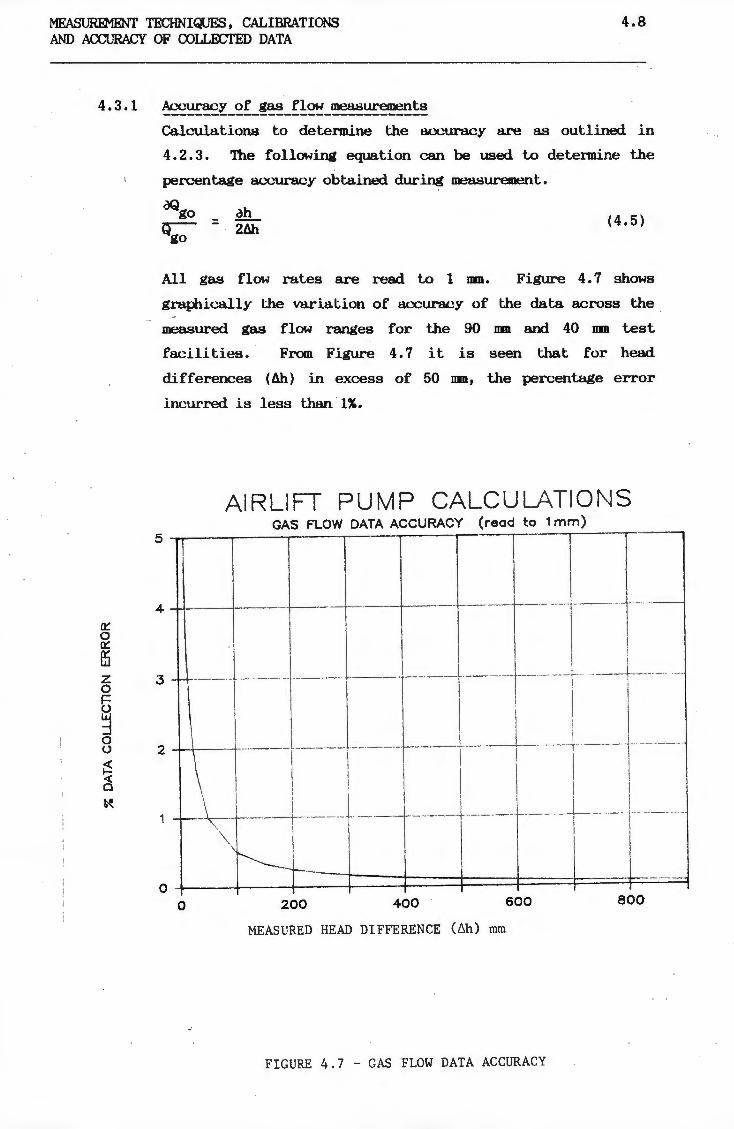
Univers
ity of
Cap
e Tow
n
' i I
MEASUREMENT TECHNI~, CALIBRATIONS AND ACCURACY OF OOLLECTED DATA
4.8
4.3.l ~~~~-~f-~~-f!~~-~~~~~~
a::: 0 a:: ffi z 0
t w :l 0 u
~ (§ ~
Calculations to determine the aocuracy are as outlined in
4.2.3. 1be following equation can be used to determine the
percentage a<...--curacy obtained during measurement.
aQgo ah = .,..-- 2Llh
~go (4.5)
All gas flow rates are read to 1 nm. Figure 4. 7 shows
gra}ilically the variation of accuracy of the data across the
measured gas flow ranges for the 90 nm and 40 DID test
5
f a.clli ties, From Figure 4, 7 it is seen that for head
differences (db) in excess of 50 um, the percentage eITor
incurred is less than · 1%.
AIRLIFT PUMP CALCULATIONS GAS FLOW DATA ACCURACY (read to 1 mm)
4
-i--o·-· --+---------1-- 1 ___ J __ . ,·--
1 I i i
.3 ---· -·· ·---J~t-1- --, ------r ----+----2 ~1 _____ 1 __ _ _ 1-----+------i------1----· -----
·~-+--1 __ J ___ J ___ tl ____ ~ ___ L ___ J __ -1--- --~~ I I
o-.1-~L-~i====t===t====i====f=====f=====:i==~ 0 200 400 600 800
MEASURED HEAD DIFFERENCE (~h) mm
FIGURE 4.7 - GAS FLOW DATA ACCURACY

Univers
ity of
Cape T
own
'· ,
MEASUREMENT TECHNI(JJF.S, CALIBRATIONS AND AOOJRACY OF OOLLECI'ED DATA
4.4 Liquid flow rate measurement
4.4.1 ~Q-~-~!~!!f~-~
4.9
Liquid flow rates are monitored using a calibrated sample
tank and a micro-switch ti.ming facility. AB the gooseneck
flow divert.er at the delivery outlet is swung fraa the return
hose to the sample tank in Figure 3. 6, the m.icro-swi. tcb is
activated which starts a stopwatch. Swinging the gooseneck
back to the re turn hose reactivates the switch and the
s-top.iatch is stopped. 1he time recorded, combined with the
volume of liquid in the sample tank, yields the liquid flow
rate.
Qt = VT/t (4.7)
where VT = voluoe of liquid in sample tank (t)
t = time of sample (s)
Qt = liquid flow rate (t/s)
Figure 4.8 shows the calibration C\ll'Ve obtained for t.he
sample tank, where the height (H) measured on a standpipe
motmted on the side of t.he tank is related to the liquid
voluoe in the tank.
4.4.2 ~Q-~-~!!!!f~-~ Liquid flow measurements on this apparatus are obtained us~
a bend meter (refer Figure 3.2) consisting of a 40 11111 P.V.C.
bend. Calibration of the bend was done using a sample tank
and readings of pressure differences were recorded on a
differential pressure manometer as in 4.2.2.
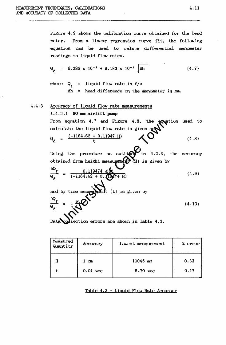
Univers
ity of
Cap
e Tow
n
MEASUREMENT TECHNIQUES, CALIBRATIONS AND ACCURACY OF OOLLECTED DATA
4.11
Figure 4. 9 shows the calibration curve obtained for the bend
meter. From a linear regression curve fi l, the following
equation CW1 be U8ed to relate dlf ferentlal manometer
readings to liquid flow rates.
Qt = 6.386 x 10- 1 + 9.183 x 10- 2 ~
where Qt = liquid flow rate in t/s
Mi = head difference on the manometer in nm.
4.4.3 ~~~-~f_!~g~~~-K!~~-~!~-~~~~!~ 4.4.3.1 90 am airlift pap
(4.7)
From equation 4. 7 and Figure 4. 8, the equation used to
calculate the llquld flow rate is given as:
= (-1164.62 + 0.11947 H) t
(4.8)
Using the procedure as outlined in 4. 2. 3, the accuracy
obtained from height measurement (H) ls given by
= 0.119474 aH (4.9) (-1164.62 + 0.119474 H)
and by time measurement (t) is given by
(4.10)
Data. collection errors are shown in Table 4.3.
Measured Accuracy Lowest measurement %,error Quantity
H 1 nm 10045 JJID 0.33
t 0.01 sec 5.70 sec 0.17
Table 4.3 - Liquid Flow RaLe Accuracy

Univers
ityof
Cape T
own
MEASUim1ENT TECHNI(\(JES, CALIBRATIONS AND Aro.JRACY OF OOI.LECTED DATA
4.12
4.4.3.2 40 .. airlift -p.mp
1he equation derived, using the procedure as outlined in
4. 2. 3, which can be used to determine the accuracy obtained
by measuring 6h on the manometers is given by:
aQt 6.386 x 10-• ah Q=
t 2 J& (6.386 x 10-• + 9.183 x 10-z Jtih)
(4.11)
Fluctuations in the manometers were averaged to 5 um. 1he
lowest measured 6h is 23 nm resulting in 0.73% error.
4.5 Static Dilation Measurement
Weber ( 1976, 1982) , in his anal ysis, requires knowledge of static
dilations discussed. in Section 2.5.6.1. Static dilations are
moni tared by direct measurement with fluctuations being averaged
visually. Equation ( 2. 34) is used to calculate the dilations 6nd
equation (4.12) is used to predict the accuracy of the measured. data.
a E. go E. go
(4.12)
It is possible to average the fluctuations of the liquid surface to
an accuracy of less than 100 um. The lowest measured tih recorded was
220 nm, with h 1 being 435 nm. 'Ibis results in a 0.3% data collection
error.

Univers
ity of
Cap
e Tow
n
MEASUREMENT TECHNIQUES, CALIBRATIONS AND ACCURACY OF COI..J..ECTED DATA
4.13
4.6 Dyruunic Vold Ratio Measurement
For calculation of the weight of lhe two phase gas-liquid eolumn
inside the delivery pipe, lt ls necessary to measure the dynamic void
ratio discussed in 2. 5 .1.1. To determine dynamic void ratios, lwo
inllne ball valves on either of the test facilities are shut off
simultaneously, trapping a collD1111 of gas and liquid. Once the gas
and liquid have separated, the ratio of pipe length cx...-cupied by air
lo total pipe length between the ball valves yields the dynamic void
ratio. Direct measurements are converted into void ratios by using
1308 - H E.g = 1376 (4.13)
on the 90 nm airlift pump, and
858 - H \~ - 909 (4.14)
on the 40 nm airlift pump
where H = the height of liquid measured to the lop of the stub
on the bottom valve in nm
= dynamic void ratio
Figure 4.10 and 3.5 show the layout and dimensions of Lhe two valves
on the 40 111n and 90 am airlift pumps respectively.
4.6.1 ~~~~-~!-~9-~~!~-~~!~-~~~~~~~ The following equations can be used to determine lhe accuracy
obtained during measurement. For the 40 nun airlift pump:
= 3 h (4.15)
(858 H ) 909 909 - 909
For the 90 am airlift pump:
= 3 h (4.16)
(1308 H ) 1376 1376 - 1376

Univers
ity of
Cap
e Tow
n
1376
(909)
H
FIGURE 4.10 -
SAS COLUMN
LIQUID COLUMN
BOTTOM VALVE
r
4. 1 i~
BRACKETS • 4'0•• AIRLIFT PUMP
BALL VALVE ARRAN&EMENT FOR DYNAMIC VOID RATIO TESTS

Univers
ity of
Cap
e Tow
n
MEASUREMENT TECHNIQUES, CALIBRATIONS AND ACCURACY OF OOI..J...ECrED DATA
Data collection errors are given in Table 4.4.
Apparatus Accuracy Lowest measurement
(H)
40 DID 1 .am 348 DID
90 nm 1 DD 382 11111
Table 4.4 - nyry,mic Void Ratio AL"CuracY
4.15
% error
1.9 x 10-•
1.5 x 10-•
Univers
ity of
Cap
e Tow
EXPERIMENTAL PROCEDURE 5.1
CHAPrER 5
EXPERIMENTAL ~
5.1 Introduction
To research analytical models for predicting airlift pump operation,
tests were conducted on both the 90 nm and 40 nJD research facilities.
During the tests, physical ~ters such as
(a) the lift height
(b) the gas injection depth
( c) gas lnjec ti on techniques
(d) gas injection apertures on the 90 nm vertical annular
gas injector
were varied. The influence of these }J6rameters on the airlift pt.UDp
operation were monitored by measurement of pressures, gas flow rates
and liquid flow rates.
Further tests that were conducted included monitoring
(a) static dilatiolli:J in 150 um, 90 nm and 40 nm pipe
diameters
(b) dynamic void ratios in 90 nm and 40 nm pipe diameters.
This chapter cove~ the experimental procedure adopted while
conducting tests to research the above effects during airlift pump
operation.
Univers
ity of
Cap
e Tow
EXPERIMENTAL PRCXEXJRE 5.2
5.2 Static dilation tests
llie static dilation discussed in Section 2. 5. 6. 1 is required for
Weber's (1976, 1982) analytical model.
To monitor static dilation, tests were perfonned in pipe s i zes:
( i) 40 lllil o. d. , 36 nm i. d.
(ii)
(iii)
90 mm o.d., 86 nm i.d.
150 IIIIl o.d., 142 nm l.d.
-The experimental procedure adopted for each pipe is as follows:
(a) Fill the pipe to a reference height (h 1 ), on Figure 2.1,
depending on the maximum dilation.
(b) Allow gas to bubble into the bottom of the pipe at a constant
rate.
( c) Record the dlla Le height ( tJl) . (d) Choose a different gas flow rate and repeat item c until the
dllationH for a range of ga8 flow rates are obtained.
Record all gas flow rates at S.T.P.

Univers
itof
Cape T
own
EXPERIMENTAL ~ 5.3
5.3 40 nm Airlift pump operating tests
5.3.1 ~~~~~~~~
Ref erring to Figure 3. 2, the following procedure is adopted
for preparing the 40 nm airlift pump for operation:
(a) Open the air release valve in the return line.
(b) Open the inline ball valves .in the delivery pipe.
(c) Open the isolation valves at all the pressure
tappings.
(d) Close the air release valves on the absolute pressure
manometers.
(e) Fill the apparatus by flushing · water through 1..he
manometers and separation pod8 into the pipe, at the
swne time priming them of air.
( f) Cl use the air release valve .in the re Lum line when
liquid flows out.
(g) Fill the constant head tank to the required lift
height.
(h) Close the isolation valves at all the pressure
tapp.ings.
(i) Set the pressure regulator on the airline to 300 kPa.
(j) Set the two way d.iverter valve to the required gas
injector.
(k) Slowly open the gas flow regulating valve, allowing
gas to enter the airlift delivery pipe.
(1) Open the isolation valves at all pressure tappings.
(m) Open the a.ir release valves on the absolute pressure
manometers.
(n) Adjust the manometerH for pressure measurement as
preseribed .in Section 4.2.1 and 4.2.2.
( o) Record all pressure readings, gas flow ra:Les and
liquid flow rates.
(
(' I
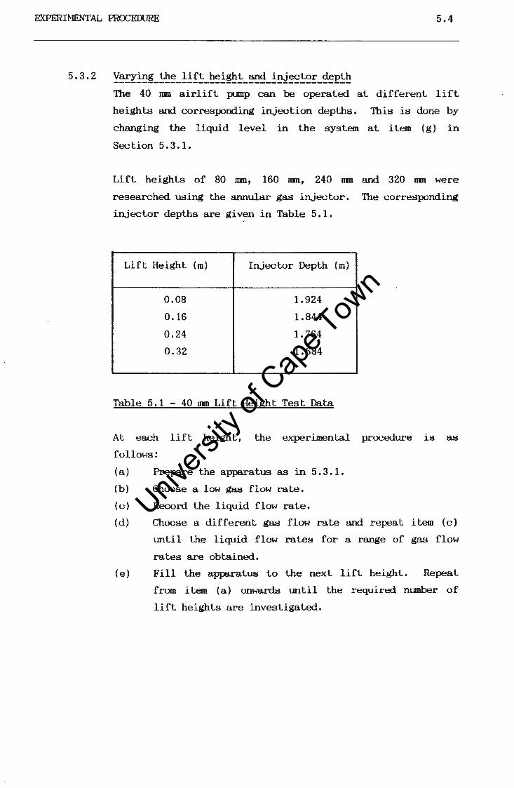
Univers
ity of
Cap
e Tow
n
EXPERIMENTAL PROCEDURE 5.4
5.3.2 Y~!~-~~-!!!~-~~!~!-~-!~J~!~E-~~P~~ The 40 nm airlift pump can be operated at different lift
heights and corresponding injection deplhs. This is done by
changing the liquid level in the system at item (g) in
Section 5. 3 .1.
Lift heights of 80 nm, 160 nm, 240 nm and 320 nm were
researched using the annular gas injector. The corresponding
injector depths are given in Table 5.1.
Lift Height (m) Injector Depth (m)
0 . 08 1.924
0.16 1.844
0.24 1.764
0.32 1.684
Table 5 .1 - 40 nm Lift Height Test Data
At each lift height, the experimental proeedw·e is as
follows:
(a) Pre~ the appu-atus as in 5.3.1.
(b) Choose a low gas flow rate.
(c) Record the liquid flow rate.
(d) Choose a different gas flow rate and repeat item (c)
until the liquid flow rates for a range of gas flow
rates are obtained.
(e) Fill the apptiralus lo the next lift height. Repeat
from Hem (a) onwa.rds until the required m.unber of
lift heights are investigated.
Univers
ity of
Cap
e Tow
n
•
EXPERIMENTAL mx::EDlJRE 5.5
5.3.3 !~J~~~~~-~~~~g~~-~~~E~~~~ To monitor the difference between hori~ontal gas injection
and vertical gas injection, test8 were eondlX!led on the two
gas injectors described in Section 3.2.3.
The tests were :nm at a 240 IlJil lift height with lhe following
operating procedure:
(a) Pre{Bre the appl!'atus as in 5.3.1.
(b) Choose the vertical annular gas injector.
(c) Choose a low gas flow rate.
(d) Record the llquld flow rate.
(e) Choose a different gas flow rate and repeat from item
(e) onwards, until the llquid flow rates for a range
of gas flow rates are obtained.
(f) Exchange the gas injectors and repeat from item (e) on
wards, now using the horizontal gas injector .
Univers
ity of
Cap
e Tow
n
EXPERIMENTAL PROCEDURE 5.6
5.4 90 mm Airlift pump operating tests
5.4.1
5.4.2
~~PY-~~~~~ Ref erring to Figure 3. 6, the fallowing procedure is adopted
for preparing the 90 am airlift pLQilp for operation:
(a) Close the drain valve at the base of the pressure
vessel.
(b) Open the inline be.11 valves in the delivery pipe.
(c) Fill the system to the required injector depth through
the constant head tank.
(d) Move the gooseneck flow diverter at the delivery
outlet to the return hose.
(e) Prime all manometers for pressure · measurement as
outlined in sections 4.2.1 and 4.2.2.
( f) Set the pressure regulator on
kPa.
the air line to 200
(g) Slowly open the gas flow regulating valve allowing gas
to enter the airlift pipe.
(h) Record all pressure readings and gas flow rates from
the manometers.
(i) ReG'Ord liquid flow rates by diverting to a sample tank
and measuring the height on a standpipe with the
sample time on a self-activated stopwatch.
~~~~~~ Tests on the 90 am airlift pump were conducted at a lift
height of 4.280 ID and an injection depth of 5.240 ID using the
following experimental procedure:
(a) Prepare the apparatus a.s in 5.4.1.
(b) Choose a low gas flow rate.
(c) Record the liquid flow rate.
(d) Choose a different gas flow rate and repeat item (c)
until the liquid flow rates for a range of gas flow
rates are obtained.
Univers
ity of
Cap
e Tow
n
EXPERIMENTAL ~ 5.7
5.4.3 ~~~~~-~~~-~~~~~E-~E!:~~~~ The 90 nm airlift pump can be operated wlth the annular gas
injector set at different aperatures. Tests were conducted at
settings 8,6 and 4 correspondlng to aperature areas of
2770.9 nm 2, 1766.36 nm 2 and 1335.2 nm 2 respectlvely (Refer
to Table 3.1)
The experimental procedure is the same as outlined in 5.4.2,
repeated for each aperature setting.
5.5 l)ynamic Void Ratio Tests
To aid in modelling the weight of the two phase mixture in the
dellvery plpe, dynamlc vold ratios were monltored ln the 40 nm and
90 nm airlift pumps.
The experimental procedure adopted for each airlift pump was as
follows:
1. Operate the airlift pump at a particular gas flow rate.
2. Record the water flow rate.
3. Record the absolute pressures at each of the two ball valves.
4. Shut the two ball valves slmultaneously trapplng a gas-liquid
column.
5. Record the height of water in the trapped column.
6. Choose a different gas flow rate and repeat from item 2
onwards until the dynamic ratios for a range of gas flow
rates are obtained.
Record all gas flow rates at S.T.P.
For the analysis, an average gas flow rate bet.ween the valves is
calculated using the air flow rate at S.T.P., the absolute pressures
al:. the two valves and equation 2 .14 The water flow rate ls obtained
directly from measurement, and the dynamic void ratio is obtained
from the ratio of air volume to total voltmie of the cohunn bet.ween
tile two valves.
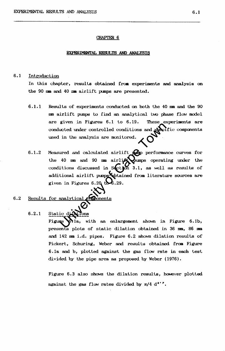
Univers
ity of
Cap
e Tow
n
EXPERIMENTAL RESULTS AND ANALYSIS 6.1
aIAPrER 6
EXl'BRIMBNTAL RmJLTS AND ANALYSIS
6.1 Introduction
In this chapter, results obtained frc.a experiments and analysis on
the 90 um and 40 IIIB alrlift ptmpS are presented.
6.1.1 Results of experiments conducted on both the 40 IDll and the 90
am airlift pumps to f lnd an analytical two Jiiage flow nvdel
are given in Figures 6 .1 to 6. 19. Th.ese experiments are
conducted lmder t..'Ontrolled condltions and specific L'OlllpOllents
used in the analysis are monitored.
6.1.2 Measured and calculated airlift pump perfonuance curves for
the 40 am and 90 am airlift pumps operating under t..he
c ondl tio~ discussed in Sec ti on 3. 1, as well as results of
additional airlift ptmpS obtained from literature sources are
given in Figures 6.20 to 6.29.
6.2 Results for analytical components
6.2.1 Static dilations
Figure 6. la, with an enlargement shown in Figure 6. lb,
presents plots of static dilation obtained in 36 nm, 86 DID
and 142 nm i.d. pipes. Figure 6.2 shows dilation results of
Pickert, Schuring, Weber and results obtained frooa Figure
6. la and b, plotted against the gas flow rate in each test
divided by the pipe area as proposed by Weber ( 1976).
Figure 6.3 also shows the dilation results, however plotted
against the gas flow rates divided by 'If/ 4 d 2 •
7•

Univers
ity of
Cap
e Tow
n
EXPERIMENTAL RESULTS AND ANALYSIS 6.2
6.2.2 ~~-~oid_E!!!~
Figure 6. 4 shows grapis of the dynamic void ratio plot led
against the average airflow rate between the two inline
valves. 'Ibe data points are compared with predictions by
Giot (1986), Chisholm (1983), Clark (1986) and Weber (1976,
1982) in the 40 DID airlift JX.lllP• Figure 6.5 is a grapi
comparing the predicted dynamic void ratios by the above
authors with the measured void ratio in the 40 11111 airlift
pump.
Figure 6.6 and Figure 6. 7 show the above for the 90 DD
airlift pump.
6.2.3 ~~!~~-P~~~~-!~~ Figure 6. 8 is a plot of the total pressure loss between the
two ball valves, during dynamic void ratio tests. Also shown
is the weight pressure loss component calculated using the
measured. dynamic void ratio results and the weight pressure
loss as calculated using the dynamic void ratios predicted by
the authors mentioned above (refer Equation 2.21).
'Ihe difference between the total pressure loss and weight
pressure los~ components consists of the friction and
acceleration pressure losses. All pressure losses are
plotted against average gas flow rates between the valves for
the 40 DID airlift pump. Figure 6.9 shows a ccmparison of the
weight pressure loss calculated using the measured. dynamic
void ratio and the weight pressure loss calculated using the
predicted dynamic void ratios.
Figure 6.10 and 6. ll show the above for the 90 na airlift
punp.

Univers
ity of
Cap
e Tow
n
\~_/
EXPERIMENTAL RESULTS AND ANALYSIS 6.3
6.2.4
6.2.5
~E!~~!~~-PE~~~~~-!~~~ Figure 6. 12 shows · the combined friction and acceleration
pressure losses as obtained from the dlffere11<...-e between the
total pressure loss and the weight pressure loss on Figure
6.8. Shown also are theoretical friction pressure loss
predictions by Chisholm (1983), Stenning (1968), Weber (1976,
1982), Clark ( 1986) and a modiflcatlon of Clark's method.
The mcxlification presented by the present author is to re
place the superficial liquid velocity Lenn ( v ls - equation
2. B) by the liquid velocity ( v l - equation 2.10) when
applying Clark's friction pressure loss equation (equation
2.45).
Friction pressure losses are plotted against lhe average gas
flow rates between the valves for the 40 nm airlift pump.
Figure 6.13 is a COlllJRI'ison of the measured data and
calculated values using the methods presented by the above
authors.
Figure 6 .14 and 6 .15 show the above results for lhe 90 IIID
airlift pump.
!~~!_PE~~~~~-!~~~ Figure 6 .16 is a plot of the total pressure loss, measured
and predicted, between the valves on the 40 nm airlift pump,
for a range of gas flow rates.
'Ibe predicted total pressure loss is calculated using
• the dynamic void ratio mcxlel presented by Clark for
the weight component (equation 2.33);
• the mcxlified Clark mcxlel for the friction component
(equation 2.45 with modification as discussed in
section 6.2.4);
• a standard two phase model for the acceleration
component (equation 2.53).
Figure 6 .17 shows a compa.rison between the measured data and
the predicted total pressure loss mcxiel.
Figures 6.18 and 6.19 show the above for the 90 lllll airlift
ptanp.

Univers
ity of
Cap
e Tow
n ' ··
EXPERIMENTAL RESULTS AND ANALYSIS 6.4
6.3 Performance Curves
The following graphs show airlift pump performance curves calculated
theoretically using the procedure outlined in Section 2. 4.
Pressure losses due to the moving two-phase mixture in the delivery
plpe are calculated using the following models:
1. Weight pressure loss component - void ratio model used by
Clark ( 1986) • . -
2. Friction pressure loss component - modification to the model
3.
6.3.1
6.3.2
6.3.3
used by Clark.
Acceleration pressure loss component - standard two phase
model.
~~~~!-~~~!!~-~~~~ Figure' 6.20 is a graph of measured and theoretically calcu-
lated liquid flow 1-ates for a range of gas flow rates ln the
40 lllD airlift pump. A comparison of the measured and
predlcted liquid flow rates is glven in Figure 6.21.
Figures 6. 22 and 6. 23 show the above comparisons for the
90 nm alrlift pump.
~2-~-~!E!!f ~-~P.:~~~!~_!!!~-~-!~~~~~E-~~P!~-~~!~~!~~ Figure 6.24 shows a comparison of the measured and predicted
llquid flow rates in the 40 um airlift pump opera.Ung at
various lift heights and corresponding injector depths as
outlined ln Section 5. 3. 2. Theoretically predlcted llquid
flow rates are plotted against measured liquid flow rates.
!2_~-~!E!!~~-~II?:!~J~~!~~-~~~!9~~-~~~!~~~ Figure 6.2.5 shows the 40 nm airlift pump perfoI'lllWK,--e curves
for the two types of gas injectors installed on the system.
Plotted are liquid flow rates ~alnst gas flow !'ates for the
horizontal gas injectors and the vertical annular gas
injector. The experimental procedure is outlined in Section
5.3.3.

Univers
ity of
Cap
e Tow
n
EXPERIMENTAL RESULTS AND ANALYSIS 6.5
6.3.4 ~2-~-~!E!!f !_~I.>:!~J~!!~~-~~!'!~~-~~!~!!~~ The results of lhe experiments outlined in Section 5.4.3 are
given in Figure 6.26. Measured liquid flow rates are plotted
for a range of gas flow rates at the three aperture areas
used for experiments.
6.3.5 ~~!!~-~~~~-~!~_!!!~~!~~-~~~~~-~~~-~!!-!!_!-!!~
PE~~~~~-~!~~!~ -
Figures 6. 27, 6. 28 and 6. 29 show compil'isons of liquid flow
rate data to calculated liquid flow rates for various pipe
sizes. 1he data is obtained from literature sources and was
presented by Clark, Gibson and Weber respectively.
1he operating conditions and airlift pump pipe diameters are
given on the figures.

Univers
ity of
Cap
e Tow
n .:·-...~
'
z 0
~ 0
80
0
6.6
AIRLIFT PUMP TEST RESULTS STATIC DILATION
36mm
142mm
~f____, ----+--·---- -
-----,-----i----
I
-----+-------+-
20 40
AIRFLOW l/s
FIGURE 6. 1a
AIRLIFT PU M P TEST RESULTS STATIC DILATION
2 4 6 8 10
AIRFLOW l/s
FIGURE 6. lb

Univers
ity of
Cap
e Town
6.7
AIRLIFT PUMP TEST RESULTS STATIC DILATION TESTS
100
90
80 ~
I
+ 70
I "O 60 .,_,,
0 0 + -t A + 1 j
0 .~ + - n +
0 Lix - I.
x K + ¢<> A
~
0 + v
'-... x I. <> I 50 "O
. --0XU +
v
¢
z 40 0
~ 30 0
20
;)E 6
I x
O< <> -x <>
·- -·->-·- 36mm UCT - - -
0
~ + 86rrm UCT ,_ <> ·--- ·-- ~ 142mm UCT - --1-v
10 ~ I
[). 47mm SCHURING ----· x 1 O'.Jmm PICKERT --\1 300mm WEBER
0 I I
I I
0 2 4 6
AIRFLOW I (P l * d ....... 2 I 4) m/s
FIGURE 6.2
AIRLIFT PU MP TEST RESULTS STATIC DILATION TESTS
100
90 ,. '
80 ~
I
+ 70
I "O 60 .,_,,
'-... I 50 "O
z 40 0
~ 30 0
20
I
1.d+.1 0.-- ----I
I --ll 'A
+ -'-- n
x 0 u ~A
-~_L<f:<f1 I I I
i r-x <> ll . xrtu
I
I I 6 I
x i
I ~ I I - a: 36mm UCT -;; + 86mm UCT _<> 0 142mm UCT ·-,.
[). 47mm SCHURING I
10 x 100mm PICKERT _ v 300mm WEBER
0 I I I I
0 20 40 60
AIRFLOW I 'Pl • d ....... 2. 7 I 4) m0•3 /s
FIGURE 6 .3

Univers
ity of
Cap
e Tow
n
100
90
80
~ 70
0
~ 60 0::
0 50 6
> ()
40 ::!: <{ z
,,_,.! >- 30 0
2 0
10
0
100
i_ ) 90
80
70
0 60 w f-
:5 50 ::::> 0 _J <{
40 0
30
20
10
0
6.8
AIRLIFT PUMP TEST RESULTS 40 mm DYNAMIC VOID RATIO COMPARISONS
- ·-- - --· ---!----+-----+- - ·-----r--- - --t--
-··-- - ·- ----- - ---1------i
0 2 3 4
AIRFLOW l/s
FIGURE 6.4
AIRLIFT PUMP TEST RESULTS 40 mm DYNAMIC VOID RATIO COMPARISONS
- ---+---+---- ·----
0 20 40
WEBER + CLARK
C GIOT & CHISHOLM
-------··- ·------..----~- ·--- ·
60 80
TEST DATA
FIGURE 6.5
100

Univers
ity of
Cap
e Tow
n
6. 9
A IRLIFT PU tv1P TFST RESU LTS 90 mm DYNAM IC VOID RATIO COMPARISONS
100
90
80
~ 7 0
0
~ 60
a 50 6 > u 40 ~ <{ z 30 >-a
. 1 . .-' 20
10
0 0 4 8 12 16 20 24 28
AIRFLOW 1/ s
FIGURE 6.6
AI RLI FT PU MP TEST RESU LTS 100
90
' 80 / /
7 0
a 60 w
~ 50 :J u _J
() 40
30
o GIOT & CHISHOLM 20 __ ,,_ --l---t---.. -- ---10
0 0 20 4 0 60 80 100
TEST DATA
FIGURE 6.7
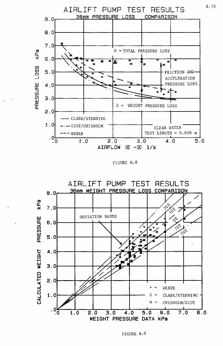
Univers
ity of
Cap
e Tow
n
ro a. ~
en en 0 _J
UJ a: ::J en en UJ a: a.
ro a.
AIRLIFT PUMP TEST RESULTS 9.0 36mm PRESSURE LOSS - COMPARISON
8.0
7.0 If
'\. o =TOTAL PRESSURE LOSS
6.0
5.0
4.0
'\.). -- -
""'~ m • • m Ji m
I ... m m
I'- m m m m ,. ......... ~
~ FRICTION AND-
ACCELERATION ......... . -- ~ PRESSURE LOSS . ........... . ~ ~· j
--~ . ,__ .--. ~ ---- •
3.0 ti = WEIGHT PRESSURE LOSS
2.0 ~ CLARK/STENNING
1. 0 -· - GIOT/CHISHOLM CLEAR WATER ---WEBER TEST LENGTH = 0.909 m
·~o 1. 0 2.0 3.0 4.0 5.0 I
AIRFLOW (E -3) l/s
FIGURE 6.8
AIRLIFT PUMP TEST RESULTS a.o--~3=6~m=m..........._W~E~I~G~H~T........,..PR~E=S~S~U~R~E=--=L=O~S~S--=-""""-'-i,..........-r--....,..., __ ----.
/
~ 7.o--~--~~--~~--~~--~------
UJ ~ 6.0t--~--+~~-+-.......... ~-+-~~+-~.....,.......-.~_,..... en en UJ a: 5.0~~--+~~-+~~~~~+'::ic~-=-f=-1~--+-'~--~--a.
~ 4.0~~--+~~-+~~-+-----::~..-"7"'!1--1'-~--+~~-+~~~ (!) H
~ 3.01--~--+~~-+__.'-'_,._ ... ~=1-~~...._~--+~~-+~~~
0 UJ ~ 2.0 ....J ::J u ....J 1.0~~-?ff~~-+~~-+-~~+-~-
~ u
+ = WEBER
ti = CLARK/STENNING
D = CHISHOLM/GIOT
·~o 1.0 2.0 3.o 4.o 5.o 6.o 1.0 a.o WEIGHT PRESSURE DATA kPa
FIGURE 6.9
6. 10

Univers
ity of
Cap
e Tow
n
12.0
11.0
10.0
cu 9.0 a. ::,[, 8.0
~ 7.0 0 _J 6.0 UJ ~ 5.0 U)
~ 4.0 a: a. 3.0
cu a. ::,[,
UJ a: => U) U) UJ a: a. t-:I: C!> H UJ x CJ UJ t-< _J
=> tJ _J
< tJ
2.0
1. 0
·~o
11.0
10.0
9.0
8.0
7.0
6.0
5.0
4.0
3.0
2.0
1.0
AIRLIFT PUMP TEST RESULTS 6 . 11
86mm PRESSURE LOSS COMPARISON
............ ..........
m ........... ......... D = TOTAL PRESSURE LOSS
~ • ........ -~m -
" • a m -._ -m.. ,,,,,.- . --- ·~- -- m ·- r--- • - -~ FRICTION AND --....,
::----.__ ACCELERATION • •. r-.._ ~
- PRESSURE -6 = WEIGHT PRESSURE LOSS LOSS -
~ CLARK/STENNING
- · - GIOT/CHISHOLM CLEAR WATER
-- WEBER TEST LENGTH = 1.376 m I .
10.0 20.0 30.0 AIRFLOW (E -3) 1/s
FIGURE 6.10
AIRLIFT PUMP TEST RESULTS 86mm WEIGHT PRESSURE LOSS
+ = WEBER
6 = CLARK/STENNING
o = CHISHOLM/GIOT
·?o 1.0 2.0 3.o 4.o 5.o 6.o 7.o 0.0 9.o 10.011.0 WEIGHT PRESSURE DATA kPa
FIGURE 6 . . 11

Univers
ity of
Cap
e Tow
n
AIRLIFT PUMP TEST RESULTS
CLEAR WATER IU Q. TEST LENGTH = 0. 909 m ~ 4.0t--~~~-+-~~~~t--~~~-+-~~~~~~~~-1
en MODIFIED CLARK en 0 ...J w 3.0t--~~~-+-~~~~t--~~~-1-~ ........ ...._~~~~~-1 ~ ~ . ~ v en s<\)~ • f3 ~~1.>s • ~ 2.0--~~~--~~~o~ •• z 0 H r u H ~ l1.
IU a. ~
w ~ ~ en en w ~ a.
z 0 H r u H ~ l1.
0 w r < ...J ~ u ...J < u
~~~G I
• CHISHOLM -----
-+--STENN ING
CLARK/WEBER
·?o 1.0 2.0 3.0 4.0 5.0 AIRFLOW (E -3) 1/s
FIGURE 6.12
AIRLIFT PUMP TEST RESULTS 5.o--~3~6~m=m----.F~R~I~CT~I~O~N---P~R~E~S~S~UR~E=--=L~O~S~S~=:..:.:...-.:.;:..:~~-
4.0
3.0
2.0
1.0
·?o
+ + +
.+ + o = STENNING +•
,,,,· ... •• ........
6 = CLARK/WEBER
+ = CHISHOLM
x =MODIFIED CLARK
1.0 2.0 3.0 4.0 5.0 FRICTION PRESSURE DATA kPa
FIGURE 6.13
6. 12
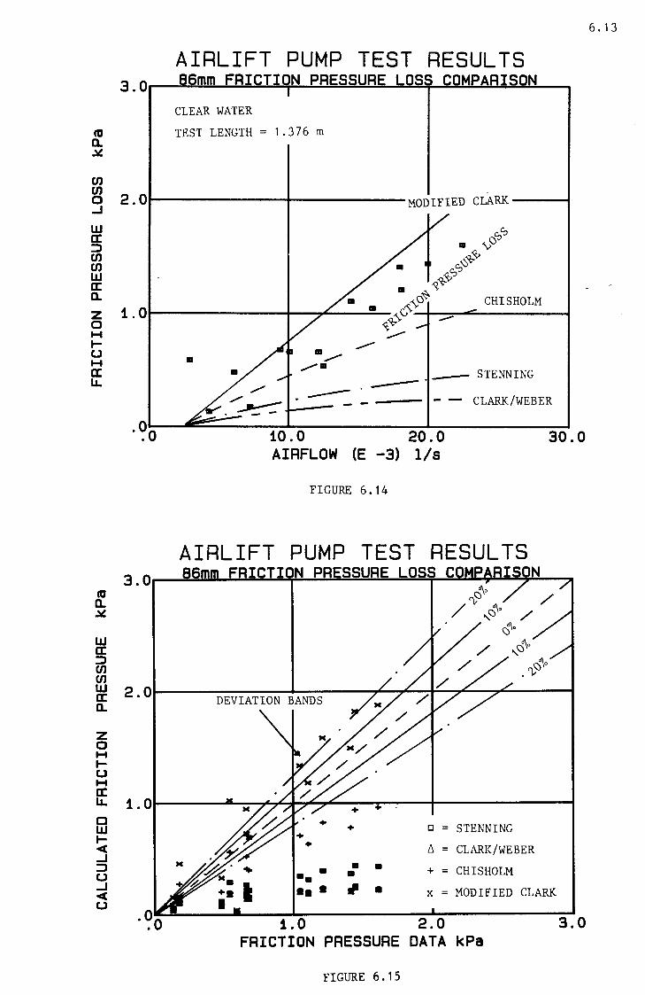
Univers
ity of
Cap
e Tow
n
IU a. :,/..
en en 0 ...J
UJ cc ::> en en UJ cc a. z 0 H t-u H cc u.
UJ cc ::> en en
3.0
2.0
1.0
·?o
AIRLIFT PUMP TEST RESULTS 86mm FRI ass COMPARISON
CLEAR WATER
TEST LENGTH = 1 .376 m
MODIFIED CLARK
sS .. '\>\)
<0'Q;-<v x_,SS .. \)~ ~~
CHISHOLM .. ~'\; '\-G -~'Q;-.....-.....-
• .. .,......,.. ,,........
- STENNING -. --- CLARK/WEBER - -10.0 20.0 30.0 AIRFLOW (E -3) l/s
FIGURE 6 .14
AIRLIFT PUMP TEST RESULTS
~ 2.0~~~~~~~-+-~~~---.~ ........... ~~.......-~....,....~~~-t a.
·?o
+
• •• •• •
+
.. . .. ~ .
o = STENNING
6 = CLARK/WEBER
+ = CHISHOLM
x = MODIFIED CLARK
1.0 2.0 FRICTION PRESSURE DATA kPa
FIGURE 6.15
3.0
6. 13

Univers
ity of
Cap
e Tow
n
ca a.
6. 14
AIRLIFT PUMP TEST RESULTS
~ 6.0t--~~~~-r-~~+----4~~---~----"""FT--~~~
CJ] ... ...
DATA ~ 5.011--~~~+-~~~-+-~~~-+-~~~-+-~~~--1 _J
~ 4.011--~~~+-~~~-+-~~~-+-~~~-+-~~~--1
::J CJ] ~ 3.0t--~~~~~~~+-~~~-+-~~~-t-~~~--1
cc Q.
2.0
1.0
·?o
9.0
ca a. 8.0 ~
UJ cc ::J CJ]
7.0 CJ] UJ cc Q.
c 6.0 UJ I-c( _J ::J u
5.0 _J c( u
CLEAR WATER WEIGHT,FRICTION & ACCELERATION PRESSURE LOSSES TEST LENGTH = 0.909 m
1.0 2.0 3.0 4.0 AIRFLOW (E -3) l/s
FIGURE 6.16
AIRLIFT PUMP TEST RESULTS
/ /
<:::>"\·
/
/
5.0
/
/
5.0 6.0 7.0 8.0 9.0 PRESSURE DATA kPa
FI GURE 6 .17
Univers
ity of
Cap
e Tow
n
12.0
11.0
10.0
ID 9.0 a. :ii. 8.0
~ 7.0 0 ...J 6.0 w § 5.0 Ul f3 4.0 a: a. 3.0
2.0
1.0
--
·~o
m a. 9.0 :ii.
w a: ~ Ul 8.0 Ul w a: a.
0 7.0 w .,_ oC( ...J ~ u
6.0 ...J oC( u
AIRLIFT PUMP TEST RESULTS -- -- =~c• ice LOSS rn~ OAR ISON .......
.. --...__ .. THEORY
/ ...--..... .....__ I ~
...... - &
- - .. , -
CLEAR WATER WEIGHT, FRICTION & ACCELERATION PRESSURE LOSSES TEST LENGTH= 1.376 m
10.0 AIRFLOW
FIGURE 6.18
20.0 CE -3) 1/s
DATA
AIRLIFT PUMP TEST RESULTS
/
/ /
6. 15
30.0
/
6.0 7.0 8.0 9.0 10.0 PRESSURE DATA kPa
FIGURE 6.19

Univers
ity of
Cap
e Tow
n
6. 16
AIRLIFT PUMP CALCULATIONS 1. 0 36mm - OPERATING CURVE
I I
CLEAR WATER ~ LTFT HEIGHT = 0.24m .9
INJECTOR DEPTH = 1.764m Ul • 8 - PIPE DIAMETER = 0.036m
..........
-(T) I
LU
3: 0 _J LL
0 H ::::> CJ H _J
ID
' ,... -(Tl I
UJ -:E 0 ..J lL
c H :::> Cl H ..J
c UJ I< ..J :::> u ..J < u
.7 ,...- m m m Ill m
/ m mm m m -/m D = DATA
I - -
m/ I
.6
.5
.4
.3
.2 THEORETICLE PREDICTIONS:
. 1 \·JEIGHT - CLARK FRICTION -MODIFIED CLARK
·~o ACCELERATION - TWO PHASE MODEL
1.0 2.0 3.0 4.0 AIRFLOW S. T. P. (E -3) 1/s
FIGURE 6.20
AIRLIFT PUMP CALCULATIONS
CLEAR WATER . 9 LIFT HEIGHT = 0. 24m
INJECTOR DEPTH= 1.764m PIPE DIAMETER = 0.036m .B
.4
.3
.2
. i
DEVIATION BANDS.
5.0
·?o . i .2 .3 .4 .5 .6 .7 .B .9 i.O LIQUID FLOW DATA (E -3) l/s
FIGURE 6.21

Univers
ity of
Cap
e Tow
n
6. 17
AIRLIFT PUMP CALCULATIONS
CLEAR WATER LIFT HEIGHT = 4.28m
7. 0 INJECTOR DEPTH = 5. 24m SUCTION PIPE LENGTH= 1.31m
m PIPE DIAMETER = 0.086m ' 6.0 ....... ------.--~~~~~ ---+--------+--------1 .... -('IJ 5.0 I
• • • • •
UJ D = DATA - 4.0 :z 0 ...I IL 3.0 -c .... => 2.0 a .... ...I THEORETICLE PREDICTIONS
1.0 t---P----+ ___ .....,.._ WE I GHT = CLARK
·~o
FRICTION = MODIFIED CLARK ACCELERATION = TWO PHASE MODEL
10.0 20.0 30.0 40.0 50.0 AIRFLOW S.T.P. (E -3) 1/s
FIGURE 6 .22
AIRLIFT PUMP CALCULATIONS
CLEAR WATER m LIFT HEIGHT = 4.28m :::. 7 .0 INJECTOR DEPTH = 5.24m
SUCTION PIPE LENGTH= 1.31m ii1 PIPE DIAMETER = 0.086m I 6.0
UJ -
1.0 2.0 3.0 4.0 5.0 6.0 7.0 8.0 LIQUID FLOW DATA (E -3) 1/a
FIGURE 6.23

Univers
ity of
Cap
e Tow
n
CIJ
' .... -('I) I
UJ -x 0 ...I lL
c .... :J Cl
- - .... ...I
c UJ I-~ ...I :J u ...I ~ u
1
0.9
o.e
0.7
~ 0.8
~ o.e
~ 0.-4
31: 0.3
0.2
0.1
0
1.0
.9
.B
.7
.. 6
.5
.4
.3
.2
. 1
AIRLIFT PUMP CALCULATIONS 36mm -
+ 0.08/1.924 6. 0.16/1 .844 0 0.24/1.764 0 0.32/1.684
DEVIATION BANDS
CLEAR WATER
6 . 18
.1 .2 .3 .4 .5 .6 .7 .B .9 1.0 LIQUID FLOW DATA (E -3) l/s
FIGURE 6.24
AIRLIFT PUMP TEST RESULTS 40mm INJECTOR TYPE COMPARISONS
-
1 VERTICLE INJECTOR
I - - - --;
~ ..... . :"'
~ ICI"" . ... ... . i,...--r
~ HORIZONTAL INJECTOR
11· T
CLEAR WATER LIFT HEIGHT = 0.24m -INJECTOR DEPTH = 1 .764m
' · PIPE DIAMETER= 0.036m I I I I
0 2
AIRFLOW I/•
FIGURE 6.25

Univers
ity of
Cap
e Tow
n
m
' ,... -(IJ I
UJ -:s
6. 19
AIRLIFT PUMP TEST RESULTS 90mm INJECTOR APERTURE VARIATION
8...,----r------,r-----..----..--------y-----T-----
D
CLEAR WATER LIFT HEIGHT = 4.28m INJECTOR DEPTH = 5.24m
3 -+---+-i11r+----41----+---+-- SUCTION PI PE LENG TH = 1 . 3 1 m PIPE DIAMETER = 0.086m
APERATURE AREA 1 -+---+-----41----+-\--+-- o = 8 ( 277 0. 9mm~)
+ · = 6 (1776.4mm27 ~ = 4 (1335.2mm)
0 10 20 30
AIR FLOW_ (I/•)
Figur e 6 . 26
AIRLIFT PUMP CALCULATIONS
3.24m 14.06m
Om 0.0381m
~ .6
,3, ....... -+--~~~""'"'+-~-+----+---+----t--t------1
.211---+-~~~~~-+---+~-+---+-~f----+-----t
.1~-n-~;..._+---+---+---t-~- DEVI ATION BANDS
.1 .2 .3 .4 .5 .6 .7 .a .9 1.0 LIQUID FLOW DATA (E -3) l/s
FIGURE 6. 2 7

Univers
ity of
Cap
e Tow
n
DISCUSSION 7.1
CHAPI'ER 7
DI~I~
7.1 Introduction
In this chapter, the results obtained from experiments and analysis
on the 40 DIB and 90 11111 airlift purnp8 are discussed. 'These include
the following component results used for the analytical model:
• STATIC DILATI<:m
• DYNAMIC VOID RATICS
• WEIGHT ~ ~
• FRICTI~ ~ L03SF.S
• 'IUfAL~~
Also discussed are perfo:nna.nce curves for the 40 IllD and 90 nm airlift
pumps operaLlng under the condlLlons outlined in Section 3.1 as well
as additional operating curves for airlift pumps presented in the
li Lera ture.
7.2 Component Results
7.2.1 Static dilations
Referring to Figures 6 .1 (a) and (b), static dilations
increase with increasing ga.s flow. At first the dilations
increase rapdily and then tend to level oul at higher gas
flow rates. 'Th.e staLlc dllaLlons investigated in the 36 lllll,
86 lllil and 142 111n pipe sizes all tended lo level out at
approximately 80%. TI1is would indicate that a maximum volume
concentration of gas can be enclosed in a slalic column of
liquid and gas.

Univers
ity of
Cap
e Tow
n
DISCUSSION 7.2
Figure 6. 2 shows the method pre8enled by Weber ( 1976) where
the ga8 flow rate is divided by the pipe area in Wl attempt
to produce a combined curve applicable to all pipe sizes. It
i.s noticed that the pipe sh:es researched., as well as addi
tional pipe size data obtained. from the literature do not.
combine well onto one curve.
Dividing the gas flow rate n/4 d 2 • 7 , results in reducing the
curves for the different pipe sizes to one curve, with the
maxilm.a dilation rea&ining approxi.JE.tely SOX. It will
however be shown in seclicn 7. 2. 2 that th.is is not required
for the proposed analytical model.
7.2.2 ~!~-~~!~-~~!~~ Referring to Figure 6.4, at lower gas flow rates on the 40 DID
airlift pump, the d,ynamlc void ratio is best predicted using
Clark's method. However, as the gas flow rate increases
either Weber, Giot, Chisholm or Clark could be u.sed to
calculate the dynamic void ratio.
On the 90 Illll airlift pump (Figure 6.6) Weber under-predicts
the dynamic void ratio at all gas flow rates. Again Clark
proves the most ac-curate at low gas flow rates with
Chisholm's and Giot's predictions better at higher gas flow
rates.
From a plot of calculated dynamic void ratios versus measured.
dynamic void ratios, for the 40 um airlift pump (Figure 6.5),
it is seen that most of Clark's predictions lie within 10% of
the measured data. A large number of Weber, Giot and
Chh1holm's predictions tend to lie outside 10%.
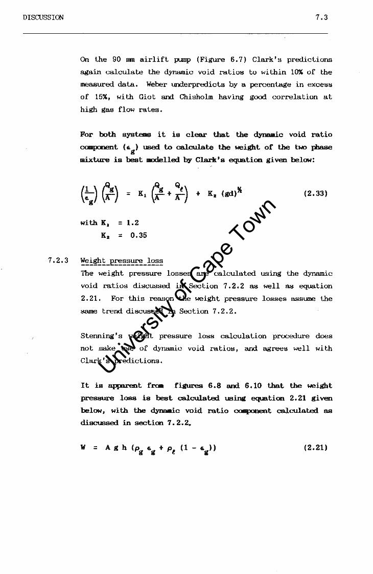
Univers
ity of
Cap
e Tow
n
DISCUSSION 7.3
On the 90 um air lift pump (Figure 6. 7) Clark's predictions
again calculate the dynamic void ratios to within 10% of the
measured data. Weber tmderp:i-edi.cts by a percentage in excess
of 15%, with Giot and Chisholm having good correlation at
high gas flow rates.
For both systems it is clear that the dyneaic void ratio
caaponent <~g> used to calculate the weight of the two }ilase
mixture is best modelled by Clark's equation given below:
with K 1 = 1.2
Ka = 0.35
(2.33)
7.2.3 ~~!~~-E£~~~~-!~~~ The weight pressure losses are calculated using the dynamic
void ratios discussed in Section 7. 2. 2 as well as equation
2.21. For this reason the weight pressure losses assune the
same trend discussed in Section 7.2.2.
Stenning' s weight pressure loss calculation procedure does
not make use of dynamic void ratios, and agrees well with
Clark's predictions.
It is apparent fraa figures 6.8 and 6.10 that the weight
pressure loss is best calculated usinli equation 2.21 given
below, with Uie dynaa.ic void ratio caaponent calculated as
discussed in section 7. 2. 2 ..
(2.21)

Univers
ity of
Cap
e Town
DISCUSSION
7.2.4
7.4
Referring to Figures 6.8 and 6.9, the difference between the
total pressure loss and the weight pressure loss consists of
friction and acceleration pressure loss components. This
differeru....'e is small at low gas flow rates, and increases at
higher gas flow rates, where friction effects tend to become
increasingly predominant.
On th.e 40 nm airlift pump, the friction and acceleration
effects contri1ll!te up to 46% of the total pressure loss
(Figure 6.8) at high gas flow rates. On the 90 nm airlift
pump, these effects only contribute 26% (Figure 6.10).
The trend of Lhe total pressure loss component is to decrease
rapidly at low gas flow rates with levelling out at higher
gas flow rates. 'Ibis is due to a low percentage of gas at
low gas flow rates, with the pressure loss t..'OOlponent made up
primarily of the weight of the liquid. As the gas flow rate
is increased, the weight of the liquid decreases resulting in
a decrease in the pressure loss. Inch.ded also is an
increasing influeru....-e of the friction and BL""Celeration
components resulting in the levelling out of the total
pressure loss.
~!~!!~~-PE~~~~-!~~~ Figures 6.12 and 6.14 show the friction and acceleration
pressure loss components of both the 40 nm and 90 IIIJl airlift
pumps. However, the acceleration component is in the order
of 1% of the total pressure loss in this case, and is not
significant.
Considering the friction pressure loss component as being the
difference between the total pressure loss and the weight
pressure loss, it is noticed that the literature under
predicts across the entire gas flow range (Figures 6.12 and
6. 14) .

Univers
ity of
Cap
e Tow
n
DISCUSSION 7.5
The trend of the friction pressure loss curve is to increase
due to a faster liquid velocity with increasing gas flow
rate. It is expected that the friction pressure drop tends
to level out slightly at higher gas flow rates B..Y the total
pressure loss and the -weight pressure loss caaponents level
out.
'lbe modi.ficaticn to Clark's calculati<n procedure, presented
- by the present author and discussed in Secticn 6.2.4, terds
to predict the fricti<n pressure loss oc1111•inent with hi...cher
accuracy cm both air lift :pmps. Referri.nli to Fi.aUres 6 .13
and 6.15, predictioos with the modified method tend to lie
within a 20S band of the measured data, .merea& methods used
in the li terat.ure show poor oorrelaticms. 'lbe fricticn
pressure OC"IOV!Dt can thus be calculated usi.IC:
6'>r = (7 .1)
7.2.5 !~~-E~~~-!~~ Both Figures 6 .17 arrl 6. 19 show how pressure losses are
calculated to within 10% of the measured data across the
entire gas flow range.
<:n both the 40 IDB and 90 DID airlift pllDp8 the calculated
total pressure loss component a.ssunes the trerd discussed in
Section 7.2.3.
Fi.Jtures 6 .16 and 6 .18 shoiw that the total iressure loee of
the gas-liquid llixture in the delivery line is adeqtate.ly
predicted, us.iJC the ocmponent results discussed in Secticn
6.2.5. and the equaticm aiiven below:
(2.16)

Univers
ity of
Cap
e Tow
n
)
DISCUSSION 7.6
7.3 Airlift Pump Perfonnance Curves
7.3.1 ~~~~!-~~~~~~-~~~~ From Figures 6. 20 a.rd 6. 22 it can be concluded that the
calc""Ulation procedure outlined in Section 2. 4 U8ing the two
phase pressure loss models discussed in Section 6. 3
adequately predicts both the 40 nm and 90 nm airlift pump
perfonnance curves.
Both graphs exhibit the characteristic airlift pt.mp operating
curve shape. With increasing gas flow rate, the liquid flow
rate first increases rapidly and then tends to flatten out to
a maximum liquid flow level characteristic of each system.
The ma.ximtml liquid flow rate is maintained as the gas flow
rate is increased and tends to drop off at extremely high gas
flow rates.
This behaviour is due to the interaction between the weight,
friction and acceleration pressure losses and is analogous to
the discussion given in Section 7. 2. 3. The maximllD liquid
flow rate obtained in any airlift ptlllp is dependent on the
system characteristics:
• lift height
• gas injection depth
• pipe diameter
• suction pipe length
• gas flow rate
• liquid and gas properties
At low gas flow rates in the 90 nm airlift pt.mp, liquid flow
rates are slightly underpredicted to within 20% of the
measured data. However, a large majority of the predicted
liquid flow rates lie within 5% of the measured data.
Fram Figures 6.21 and 6.23 it can be seen that the calcu
lation procedure used, adequately predicts liquid flow rates
in the 40 - and 90 - airlift ?JlllP8 to within 1~ of the
measured data.

Univers
ity of
Cap
e Tow
n
. "' . ·'
DISCUSSION 7. 7
7.3.2 !Q_~-~Eli!~-~~~!!~_lif!_~-!~~!~!-~P~-~!~!!~ Ref erring to Figure 6. 24, the majority of the calculated.
liquid flow rates lie within 10% of the measured data for the
lift heights and injector depths researched. 'nie calculation
prcx,~ure used tends to tmderpredict the liquid flow rates by
a small percentage.
Being a recirc..'Ulating system, various other SIE.1.1 effects
might influence the analysis which have not been accounted.
for, thus causing this slight under-prediction.
7.3.3 !Q_~-~!E!!f~~!!!J.~~!~-~~!~-~!!~ Referring to Figure 6.25, the vertical annular gas injector
tends to lead to slightly larger liquid flow rates than the
hori:wntal injector through holes. At its maximt.n, an
increase of 5% was noticed on the 40 DID airlift ptnp. 'Ihis
increase in liquid flow tends to diminish at lower airflow
values.
7.3.4 ~Q-~-~!E!!!!_~!~~~!-~~~!~ Referring to Figure 6.26, increasing the aperture area on the
vertical annular gas injector tends to lead to an ~rease in
the liquid flow rate.
'niis effect shows up to be more predominant at low gas flow
rates than at higher gas flow rates, where an increased.
aperture area has little effect on the airlift pt.mp
performance curve.
Univers
ity of
Cap
e Tow
n
DISCUSSION 7.8
7.3.5 ~~~!~-~~~-~!~_!!~~~~~~-~~~~~-~~~-~!.!:!!_~~
2E~~~~~-~!~!~ Referring to Figure 6.27, Clark's data is predicted to within
20% on a 38. 1 nm air llft pump. Clark's research equlpnent
consists of a recirculating system which could cause various
secondary pressure losses to influence the airlift ptmip
behaviour. These effects cannot be included in the analysis
as not enough information is ·given in the literature.
Ref erring to Figure 6. 28, Gibson's data is predicted to
within 10% at low gas flow rates and to within 15% at higher
gas flow rates in a 78 nm airlift punp.
Weber's data for a 300 nm airlift punp (Figure 6.29)
operating at a depth of 125 m is predicted to within 10%
throughout all gas flow rates.
Both Weber's and Gibson's airlift pumps are non
recirculating, indicating a higher accuracy.
It can be concltded that the present analysis awlied to
airlift. _p.-ps researched in the literature, adeque.tely
predicts the airlift punp perfo:nmmce curves.

Univers
ity of
Cap
e Tow
n ··: ~;~ ~:, . ; •. • ..:.·r
CONCLUSIONS 8.1
CHAPI'ER 8
1. To analyse airlift pl.lllps operating in two-phase gas-liquid flow,
pressures and pressure losses have to be calculated. 'lllese include:
• static pressure gains
• pressure losses in the suction pipe
• pressure losses ·across the gas inject.or
• pressure losses in the delivery line
2. Static pressure gains and pressure losses in the suction plpe are
concerned with liquid only and can be modelled using well-accepted
methods.
3. Pressure losses across the gas injector are small with respect to the
other pressure losses encounterect in the analysis and can be modelled
using equation 2 .12.
4. Pressure losses in the deli very pipe are due to the two-phase
gas-liquid mixture. 'lllese losses consist of:
• the weight of the gas-liquid mixture
• the friction of the gas-liquid mirlure
• the acceleration of lhe gas-liquid mixture caused by the
expmsion of the gas
5. Static dilations cause airlift punps to operate. 'lllese increase
rapidly with increasing gas flow rates. A combined static dilation
curve can be obtained by dividing the gas flow rate by rr/ 4 d 2 •
7 which
would be applicable to all pipe si~es.

Univers
ity of
Cap
e Tow
n
OONCIIBIOOS 8.2
6. Knowledge of the dynamic void ratio is required. for calculating
pressure losses due to the weight of the two-phase gas-liquid mixture
in the delivery pipe. The dynamic void ratio is best predicted uei.rll&
Clark's calculation procedure (Section 2.5.5). Weight pressure
losses of the two phase mixture can then be calculated. using equation
2.21, which has given good correlation with measured data on two
research facilities.
7. Pressure losses due to the friction of the two piase mixture in the
delivery pipe becomes increasingly significant at high gas flow
rates. '!he losses can be predicted using a modification to Clark's
calculation procedure (section 6.2.4) developed by the present author
(equation 7. 1) •
8. Pressure losses due to the acceleration of the two-Jiiase mixture in
the deli. very pipe are small compared with weight and friction
pressure losses. 'lhese losses are adequately predicted using a
standard. two-}ilase model.
9. '!he addi. lion of the models recoomended in items 6, 7 and 8 above lead
to good prediction of the two-.Eiiase pressure losses in the deli very
pipe.
10. '!he calculatiori procedure outlined in Section 2.4 is highly suitable
for the prediction of airlift pllllp behaviour. Gocxi agreement is
obtained when using the present theory to analyse the airlift p..nps
researched at the University of Cape Tuwn as well as airlift µ.mp
data from other authors and presented in the literature.

Univers
ity of
Cap
e Tow
n
REFERENCES
1. Apazides, N. 1985
R.1
REFERENCES
Influence of bubble expansion and relative
velocity on the performance and stability of an
airlift plUilp.
International Journal of
Vol. 11(4), pp. 459 - 479.
Multiphase Flow,
2 • Alves , G. E. March Two phase flow iri pipes. Fluid and Particle
3. Blevius, R.D.
1954
1984
4. Bergeaud, F. April
1973
5. Chisholm, D. proc.
Sutherland, L.A. 1969
6. Chisholm, D. 1983
7. Clark, N.N. Jan
Meloy, T.P. 1985
Flemner, R.L.C.
8. Clark, N.N.
De.bolt, R.J.
9. Clauss, G.
10. Dedegil, M.Y.
11. Dedegil, M.Y.
12. Dedegil, M.Y.
Jan
1986
1978
June
1982
1974
1978
Mechanics, Ch. 6.
Applied fluid dynamics handbook. Van Nostrand and
Company Inc.
How to calculate air lifts for marine dredging
and mining. Ocean Industy, pp. 169 - 172.
Predlction of pres8ure gradients in pipeline
systems during two-phase flow. Institution of
mechanical engineers, Vol. 184, pe.rt 3c, pa.per 4.
Two-phase flow in pipelines and heat exchangers.
Pitman Press Ltd.
Predicting the lift of airlift plUDJ>S in the bubble
flow regime. Chem S.A., Vol. 22, pp. 14-17.
A general design equation for airlift pumps
operating in slug flow. Aiche Journal, Vol. 32,
No. 1, pp. 56-63.
Hydraulic lifting in deep=sea mining.
Marine Mining, Vol. 1, No. 3.
Increase of the suction head by means of the
"airlift" method. Bulk solids handling, Vol. 2,
No. 2, pp. 267-269.
Feststoff F(jrderung Nach Dem Lufthebe Verhahren.
Von Spe~ialisten fUr Spe~ialisten, pp. 1-5.
Entwicklungs Stand Und Tendenzen Beim
Feststoffordern Nach Dem Lufthebe Verfahren.
Maschinerunarkt, WUrzenburg, 34,39; pp.765-769.
Univers
ityof
Cape T
own
REFERENCES
13. Feld.le, G.
(dissertation)
14. Fritz, H.R.
15. Gibson, L.A.
16. Giot, M;
Berleur
17. Giddings, T.
18. Giek, K.
19. Golan, L.P.
Stenning, A.M.
20. Halde, R;
Svensson, M.
21. Hill, J .C.C.
22. Kytomaa, H.K.
Brenen, C.E.
23. Kouremenous,D.A.
Staicos, J.
24. Lazarus, J.H.
25. Lazarus, J.H.
Berg, R.R.
26. Lazarus, J.H.
Berg, R.R.
Feb.
1969
1925
Oct.
1986
1983
1979
Proc.
R.2
'llleoretische und Experimentelle Untersuchungen
Uber die Vertikale Hyeiraulische f eststaff
fljrderung nach dem Strahlpumpverfahren.
Theoretical and practical aspects of the airlift
reverse circulation boring system.
Sprengen, R.a.t.mlen.
Bohren,
The Airlift PLnnp. Hydraulics and its applica
tions, 3rd edition, Constable and Company Limited.
Application of the Airlift principal to solve
maintenance problems. Hydrotransport 10, Paper D2.
The use of airlift pumps to develop wells.
Groundwater, V.21(4), pp. 521-522.
A collection of technical formulae. 4th edition,
Geick-verlag.
Two phase vertical flow maps, Institution of
1969-70 Mechanical Engineers, Vol. 184, Part 3c, Paper 14.
1981
Dec.
1978
Dec.
1986
March
1985
Aug.
1982
March
1987
J\.llle
1987
Design of airlift pumps for continuous sand
filters.
pp.223-227.
Chemical Engineering Journal (21);
Special dredging systems. Reprint from dredging
and port construction.
Some observations of flow patterns and statisti
cal properties of three component flows.
International Symposium on Slurry Flow, pp.95-101.
Performance of a small airlift pump.
The International Journal of Heat and Flow,
Vol. 6, No. 1, pp. 217 - 222.
Pump and Pipeline Instrtnnentation.
Hydrotransport 8, Paper 14.
Airlift Pumps for Ocean Mining Application.
Research Report 1 for De Beers Marine, IITRU,
University of Cape Town.
Airlift Pumps for Ocean Mining Application.
Research Report 2 for De Beers Marine, HTRU,
University of Cape Town.

Univers
ity of
Cap
e Tow
n
r \ \. _ )
REFERENCES
27. Lazarus, J.H.
Berg, R.R.
28. Lazarus, J.H.
Berg, R.G.
29. Lazarus , J. H.
Berg, R.R.
30. Lazarus, J.H.
31. Lazarus , J. H.
32. Loomis, A.W.
33. Stenning, A.H.
Martin, C.B.
34. Stone, J.H.
35. Stanislav, J.F.
Kokal, S.
Nicholson, M.K.
36. Sheba.tin, V.G.
Sokolov, N.N.
Dornanskii , I • V.
Davydov, I.V.
37. Sheba.tin, V.G.
Domanskii, I. v. Sokolov, V.N.
38. Stenning, A.H.
Martin, C.B.
39. Stone, I.N.
40. Tong, L.S.
Jl.Ule
1987
Jl.Ule
1987
Oct
1987
July
1984
1987
1980
April
1968
1987
Dec
1986
1977
1977
R.3
Airlift Pumps for Ocean Mining Application.
Preliminary to Research Report 3 for De Beers
Marine, HTRU, University of Cape Town.
Airlift pump investigation: "Static dilation
tests". Research Report 3 for De Beers Marine,
HTRU, University of Cape Town.
Airlift pump investigation: "Dynamic void ratios".
Research Report 4 for De Beers Marine, HTRU,
University of Cape Town.
CE 302 - HYdra.ulic Engineering Laboratory Manual,
University of Cape Town.
Thesis 42 : 40 lllil Airlift Pump.
Undergraduate thesis, University of Cape Town.
Compressed Air and Gas Data. Chapter 31: Airlift
pumping. Ingersoll-Rand Company, Washington.
An analytical experimental study of airlift pump
performance. Transactions of ASME, pp. 106-110.
A program to calculate airlift pump performance.
Microsoftware for engineers; Vol. 3; No. 3.
Gas liquid flow in downward and upward inclined
~. The Canadian Journal of Chemical Engi
neering, Vol 64, pp. 881-886.
Air-lift conveying of liquids and suspensions.
Journal of Applied Chemistry of the USSR,
Vo. 50(4); pp. 823-826.
Gas content of a rising stream of three-phase
gas-liquid-solid mixture. Journal of Applied
Chemistry of the USSR, Vol. 50(4), pp. 810-814.
April An analytical and experimental study of airlift
1968 pump performance. Transactions of ASME, pp.106-110
1987 A program to calculate air-lift pump performance.
Microsoftware for Engineers; Vol. 3; No. 3.
196~ Boiling heat transfer and two phase flow.
John Wiley & Sons, Inc.

Univers
ity of
Cap
e Tow
n
REFERENCE'S
41. Unknown
42. Weber, M.
Dedegil, M. Y.
43. Weber, M.
44. Weber, M.
45. Weber, M.
Schauki, N.
1976
1982
Dec.
1976
1967
R.4
"A versatile Italian dredge pllllp sygtem".
Reprint from "World Dredging & Marine Construction
Magazine.
Transport of solids according to the airlift
principle. Hydrotransport 4, p:t.per III.
Vertical hydraulic conveying of solids by airlift.
Journal of pipelines 3; No. 2; pp. 137-152.
Das Air-lift Verfahren und Seine einselzbarkeit
zur forderung von mineralien aus der tiefsee.
Meeres technique 7, 1976, pp. 189-199.
Pneuma.tische unde hydraulische forderung.
Auf berei tungs technik; Jahrgang 8;
pp. 594-558.
NlO,

Univers
ity of
Cap
e Tow
n
APPENDIX
.. A
B
c
D
OONTENTS OF APPENDIX
O:ESCRIPl'ION
Calculation procedure and computer program
Chisholm (1983) - ArmaOO. coefficient derivation
Detailed component results
Examinations written by the author to complete
the requirements of the degree

Univers
ity of
Cap
e Tow
n
APPENDIX A
CALCULATION mxEXJRE AND CCl1R1I'ER ~
i . .~/ ~

Univers
ityof
Cape T
ownl
. ,i
APPENDIX A. A.1
APPENDIX A
1. INTIUXJCTICN
To predict the perfornence of airlift ?-lllP8 operating wxler different
conditions, it is necessary to calculate liquid flow rates for a
range of gas flow rates.
A computer program has been written in True Basic (Version 2), to aid
in calculating the liquid flow rate' for a specific gas flow rate.
'Ibis chapter describes the calculation procedure used when analysi.IC
airlift pt.mpS and gives a listing of the computer program.
2 . CALCULATION mx;EOORE
To analyse an airlift puup, the technique discussed in section 2.4 is
used. It is necessary to calculate:
( i) the static pressure at the suction inlet;
(ii)
(iii)
(iv)
the pressure losses in the suction line;
the pressure losses across the gas injector;
the pressure losses in the delivery line.
Having calculated the above four pressures, a pressure be.lance is
performed:
At.mos?ieric pressure at the external liquid level
+ static pressure gain to the suction inlet
= Atmos?ieric pressure at the external liquid level
+ pressure loss in the suction line
+ +
pressure loss across the gas injector
pressure loss in the delivery line (Al)

Univers
ity of
Cape Tow
n
i j
APPENDIX A. A. 2
1hus if lhe airlift pl.lllp is in dynamic equilibrhm, then the:
static pressure gain
= pressure loss in the suction line
+ pressure loss across the gas injector
+ pressure loss in the delivery line (A2)
and the two atmos?ieric pressures in equation Al be.lance.
For calculating the pressures in equation (A2) it is necessary to
know the gas flow rate and liquid flow rate as well as the
irrlependent variables. However, the liquid flow rate for a specific
gas flow rate is the solution to the analysis and it is necessary to
assune an initial liquid flow rate which is adjusted. subject to the
pressure balance. 1he following is the calculation procedure:
(i)
(ii)
(iii)
Input irrlependent variables (pipe diameter, gas injection
depth, length of suction pipe and height of lift).
Assune an initial liquid flow rate.
Calculate all pressures (equation Al or A2) using the assuned
liquid flow rate.
(iv) Balance equation Al.
(v) If the two atmos?ieric presures do not be.lance within a
prescribed accuracy, then adjust the liquid flow rate and
(vi)
reiterate from item (iii) above.
Continue this procedure until equaticm Al is balanced. The
liquid flow rate chosen is then lhe solution.

Univers
ity of
Cape Tow
n
APPENDIX A.
2.2
A.3
Pressure calculation
2.2.1 ~~~~~-E~_!~~-~~~ '!be static pressure gain is calculated as described in
Section 2. 4. 1.
2.2.2 Pressure losses in the suction line
Pressm-e losses in the suction line are calculated as
described in Section 2.4.2.
In the omprter proga:w, the above two pressures are
used to calculate the pressure before the gas
injecti<m point which is given by:
pressure before gas injecticn = at.Jspberic pressure
at external liquid level
+ static pressure gain to the sucticm inlet
- pressure losses in the sucticm line. (A3)
2.2.3 ~~~~~-!~~~~-~~-~-j~~~~tor
(i)
(ii)
(iii)
(iv)
Pressure loss across the gas inject.or a.re calculated
using equation (2.12) and the following procedure:
Calculate gas flow rate using the pressure at the gas
injector (A3) and equation (2. H-).
Calculate the dynamic void ratio.
Calculate the liquid and gas velocities.
Apply equa~ion (2.12).
'the pressure after the .._ injecticm point is
calculated uei.Jc
pressure after gas injecticn = pressure before gas
injecticm - pressure loss across the OS injectors
(A4)
Univers
ity of
Cap
e Tow
n
APPENDIX A. A. 4
2.2.4 ~~~~~~-!~~~-!!!-~~~!!~~!'l-P!~ Pressure losses in the delivery pipe are calculated
using equation (2.lb)
To allow for the isothermal expansion of the gas
bubble up the deli very pipe, the pressure losses are
calculated. in incremental steps and then added.
In -each incremental step the average weight and
friction are calculated.. For this reason, as well as
to calculate the act,--eleration, it ls necessary to
detennine the velocity of the gas and liquid Jiiages
and the void ratios at the beginning and errl of e&.---h
incremental step.
For the void ratios and gas velocities, it is
necessary to determine the gas flow rate at the end of
an incremental step. For this, the pressure at the
end of the incremental step is required. which is the
solution lo the calculation. To overcaoe this, the
gas flow rate and void ratio at the end of the
incremental step is aprox:imated..
This is done by calculating the void ratio at the gas
injector and delivery outlet. Assl.llling a linear void
ratio increase up the delivery pipe length, the end of
each increment can be approximated..
Various incremental steps were used and it was found
steps of 1 m length give sufficiently accurate
results.

Univers
ity of
Cap
e Tow
n
APPENDIX A. A.5
Thus the following procedure is used to calculate the
pressure loss in the delivery pipe.
1. Choose incremental step distance.
2. Calculate the dYnam.lc void ratio at the deli very
outlet.
3. Calculate void ratio increase per incremental step.
4. Calculate gas flow rate at the beginning and end of
each incremental step.
5. Calculate phase velocities at the beginning and erd. of
each incremental step.
6. Calculate average weight and friction components for
each incremental step.
7. Apply equation ( 2. 16) and calculate pressure loss
across each incremental step.
8. Sun all icnremental pressure losses up the deli very
pipe.
1be pressure at t.he delivery ouUet is calculated
pressure at t.he deli very ouUet = pressure after ~
injecti<n - total pressure loss up the deliveJrT pipe.
(A5)
2.2.5 Pressure balance ----------------1 f the initial gas flow rate chosen is c...'Orrect, lhen
the airlift :p..mp is in dynamic equilibriuo, and the
pressure at the delivery outlet should balance atnos
}'.iieric pressure to within a stipulated. acx..."1"8Cy.
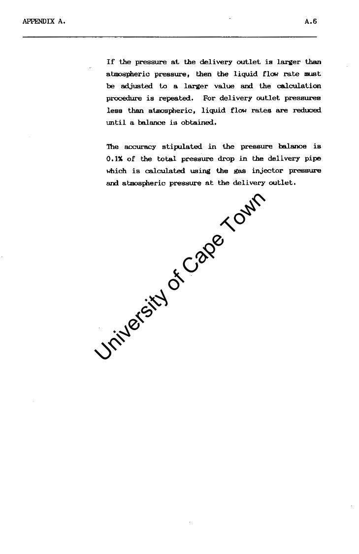
Univers
ity of
Cap
e Tow
n
APPENDIX A. A.6
If the pressure at the delivery outlet is larger than
at:mcIBJiieric pressure, then the liquid flow rate must
be adjusted to a larger value and the calculation
procedure is repeated.. For deli very outlet pressures
less than atmos:P1eric, liquid flow rates are reduced
until a be.l.anL--e is obtained.
The a.ccuracy stipulated in the pressure balance is
0.1% of the total pressure drop in the delivery pipe
which is calculated using the gas injector pressure
and atmos:P1eric pressure at the delivery outlet.

Univers
ity of
Cap
e Tow
n
ADJUST LIQUID FLOM RATE
NO
INPUT
AIRLIFT PUMP PARAMETERS REQUIRED SAS FLOW RATE
CHOOSE LIQUID 1------t FLOW RATE
PRESSURE CALCULATION
PRESSURE BALANCE
I YES I
I OUTPUT
FIGURE Ai

Univers
ity of
Cap
e Tow
n
'llltllllllllltlllllllllllltllllllllllllltlllllllllllllllllllilililllllllllll
AIRLIFT PUKP ANALYSIS progra1 to calculate operating curves in two phase flow
R R BERS 1907 111111111111111111111111111111111111111111111111111111111111111111111111111111
! SETUP ---------------------------------------------------------------------
LIBRARY "ENHANCE.TRU' di1 LIQUID!250),Qg(250l,P11!250),Eg!250),dp!250}
! INTRODUCTION SCREEN AND DATA INPUT ----------------------------------------
CALL OpeningScreen
CALL InputRoutine
! INCREHENTAL STEP DISTANCE --------------------------------------------------
LET N = INT!Hl~H2l LET COUNT = 1
CLEAR
I GAS FLOW RATE LOOP ---------------------------------------------------------
DO
! OUTPUT SCREEN --------------------------------------------------------------
CALL HiCenter !2, • HAIN CALCULATION ROUTINE ') SET CURSOR 10,1 call Hien PRINT "ENTER SAS FLOW RATE S. T.P. l/s ? SET CURSOR 10,33
INPUT QSO let Qgo = Qgo/1000
call HIOFF
CALL -DRAWVLINE!5,20,40l SET CURSOR 5,42 PRINT 'GAS FLOW RATE' SET CURSOR 6,42 PRINT • l/s S.T.P. 1
CALL DRAWhLINE!7,41,80}
SET CURSOR 5,62 PRINT "LIQUID FLOW RATE" SET CURSOR o,62 PRINT ' l/s
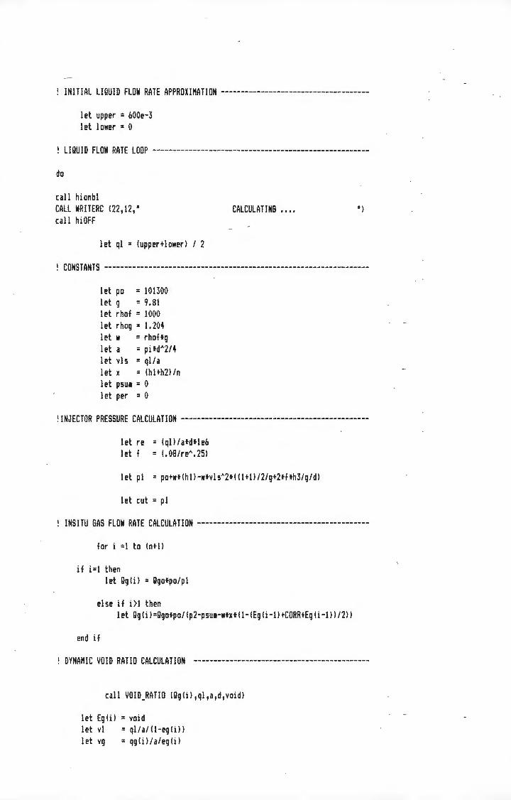
Univers
ity of
Cap
e Tow
n
INITIAL LIQUID FLOW RATE APPROXIMATION -------------------------------------
let upper = 600e-3 let lower = 0
! LIQUID FLOW RATE LOOP ------------------------------------------------------
do
call hionbl CALL WRITERC !22,12,' call hiOFF
let ql = (upper+lowerl I 2
CALCULATING •••• ")
~ CONSTANTS ------------------------------------------------------------------
let po = 101300 let g = 9.81 let rhof = 1000 let rhog = I. 204 let w = r hof •g let a = pitdA2/4 let vls = ql/a let x = (hi +h2l In let psu1 = 0 let per = 0
!INJECTOR PRESSURE CALCULATION-----------------------------------------------
let re = !qll/atdtle6 let f = !.08/reA.25)
let pl = po+wt(hli-wtvlsA2t!!1+1l/2/g+2tfth3/g/d)
let cut = pl
INSITU GAS FLOW RATE CALCULATION -------------------------------------------
for i =1 to !n+l>
if i=l then let Qg!il = Qgotpo/pl
else if i >I then let Qg!il=Qgotpo/!p2-psu1-w•x•!1-!Eg!i-ll+CORR+Eg!i-1ll/2ll
end if
! DYNAMIC VOID RATIO CALCULATION --------------------------------------------
call VOID_RATIO !Qg!il,ql,a,d,voidl
let Egli) = void let vi = ql/a/!1-eg!i)) let vg = qg!i)/a/eg(i)

Univers
ity of
Cap
e Tow
n
! VOID RATIO INCREASE PER INCRtHttfTAL ST£P _::_ _________ :.: ______ .: ___ ;: __________ . __ .
let kl = a•0.35t(9.81•dl A0.5 let k2 = k1+1.2tql let per = k2t(Qgo-Qg(1ll/(Qg(!)t(l.2tQg!ll+k2ll let corr = eg!llt(l+perl/n
PRESSURE LOSS ACROSS GAS INJECTOR -----------------------------------------
if i = I then let Qgh = !e-99 1 et Qgl = Qg ( i l
call ACCELERATION !Qgh,Qgl,ql,a,d,accl
let p2 = pl - ace
else if i>1 then
~ PRESSURE LOSSES PER INCREMENT ----------------------------------------------
end if
next i
let RE = vlstd/le-6 let F = .08/REA0.25
let FRICTION= 2000tFtxtvl A2/dt(!+1.5t(egli-ll+eg(ill/2l
let qgh = qg ( i -I l l et qg l = qg H l
call ACCELERATION (Qgh,Qgl,ql,a,d,accl
let HEIGHT=lleg(i-ll+eg!ill/2•1.204+11-leg(i-ll+eg!ill/2l•1000ltgtx
let dplil=FRICTION+HEI GHT+ACC
let psu1=psu1+dp(i)
let p3 = p2-psu1
~ PRESSURE BALANCE -----------------------------------------------------------
loop
let' 1 eft = po let right = p3 let bal = left - right
if abs!ball < !!CUT-pol•.OO!l then exit do
end if
else if bal < 0 then let lower = ql
else if bal > 0 then let upper=ql
•

Univers
ity of
Cap
e Tow
n
~ OUTPUT AND SUBROUTINES -----------------------------------------------------
SET CURSOR COUNT+8,47 PRINT USING •t.tlAAA • : Qgot!OOO SET CURSOR COUNT+8,68 PRINT USING •t.llAAAI : Qlt!OOO
CALL PROMPT IF ANSS = 1 N1 THEN EXIT DO LET COUNT = COUNT + 1 LOOP
I ' If 11 Ir If I I I I 11 1 1 1 fIII111II11I1111lIIllI 1 1 1If I1 1I111111III11III II1 1I II I 1 1 1
sub VOID_RATIO (qg,ql,a,d,voidl
let void =( a•l1.2•(qg/a+ql/al+.35•(9.81•dl AO.Sl/qglA(-ll
end sub
I' 1 1 1I1111 II I I II 11111 1 rr111 I I 1 11 I l1111If111lII11I11II1111I111•t I Jt iI 1 1 I I 1 1 r
sub ACCELERATION !Qgh,Qgl,ql,a,d,accl
let Egh = ( a•(l.2•(Qgh/a+ql/al+.35•(9.8l•dlA0.51/Qghl A( -!) let Egl = ( at(1.2t(Qgl/a+ql/al+.35t(9.8l•dlA0.51 /QgllA(-ll let vlh = ql /a/(1-Eghl let vgh = QghiaiEgh let vll = ql/a/(1-Egll let vgl = Qgl/a/Egl
let pah = Egh•1.204tvghA2 + (1-Eghl•1000fvlhA2 let pal = Egl•l.204•vgl A2 + (!-Egll•lOOO•vllA2
let ace = pal-pah
end sub
I ' 111111II r 1 11 111I111I1111II11 I I fl II 1111 l 1 111 I 11111 •11 rIIIII 1 111 I r I 1 1II111 I
SUB OpeningScreen
CLEAR CALL DrawBox(2,8,10,701 CALL HiCenterl4, 1 A IR LI FT PU KP AN ALYS I S "} CALL HiCenter(b, 1 T W 0 PHASE - GAS L I Q U I D 1 )
CALL HiOff CALL WriteCenter(12, •p RED I CT I 0 N 0 F L I Q U I D"> CALL WriteCenter(14, 1 F L 0 W R A T E F 0 R A G I V E N"> CALL WriteCenter(lb, 1 G AS FL 0 W RAT E I N AN Y"l CALL WriteCenter(l8, "A I R L I F T PU K P"I CALL DrawBox(21,23,25,551 CALL WriteCenter(22,"R R Berg (cl 1988'} CALL WriteCenter(25, "Press any key to continue') GET KEY c CLEAR
END SUB

Univers
ity of
Cap
e Tow
n
11111111111111 Ir II Ill I I It 111III1111 If II I II I I If 11111IfII111111111Ilfl11 If I If
SUB InputRoutine
CLEAR CALL HiCenterl2, • CALL HiOn set cursor B,l
INPUT DATA SUBROUTINE
print "ENTER DEPTH OF THE GAS INJECTOR (1): print "ENTER STATIC LIFT HEIGHT (1): print 'ENTER LENGTH OF SUCTION PIPE (1): print "ENTER PIPE DIAllETER !1):
SET CURSOR B,36 INPUT Hl SET CURSOR 9136 INPUT H2 SET CURSOR 10,36 INPUT H3 SET CURSOR 11,36 INPUT d CALL HiOff
I)
I' fl Ill 111flII11111111 If I If I 11f111III1f111flI111111 1 If I I I 11IIf111 f ff fl I II II
CALL HiCENTER !22,"Do you need further gas flow rates? - y or n ") INPUT ANSf LET ANSf = UCASEflANSfl
END SUB
I' II 11 II fl II 11111111111J1111111111fl11 II fl I I If I 1111111lfl111111Iff11111 f ' ''
end

Univers
ity of
Cap
e Tow
n
APPENDIX B
CHISHOLM (1983) - ARMAND COEFFICIENT DERIVATION

Univers
ity of
Cap
e Tow
n · :·,
APPENDIX B B.1
APPENDIX B
<:mSIDlf'S (1983) ARMAND OOBFFICIBNT DBRIVATI~
1. Introduction
Chisholm uses equation 2.31 to calculate the Armand coefficient,
which then is used in calculating the dynamic void ratio. The
following Appendix shows how Chisholm derived equation 2.31.
2. Derlvation
The voluoe flow ratio p is glven by:
Qg (Bl.1)
The velocity ratio (K) is the ratio of average gas velocity to
average liquid velocity, given by
vg K =
The dynanmic void ratio ls given by:
Ag = A
(Bl. 2)
(Bt.3)
Fran continuity the volume flow rates of the liquid and gas phases
are given by:
(Bl. 4)
and (Bl. 5)
vg Multiplying equation (Bt.3) by , and substituting equations
vg (Bl.2), (Bl.4) and (Bl.5), the dynamic void ratio can be expressed
as:
(Bl.6)

Univers
ity of
Cap
e Tow
n
APPENDIX B B.2
Using U>.e approach presented by Armand ( 1946) for dynamic void ratio
calculation,
£. = c p g A
and substituting equation (Bl.6) results in
1 K Qt p c = p + Q A g
Further substitution of equation (Bl.1) results in:
-1. = p + K( 1 - p) CA
For the calculation of K, Chisholm uses
K = 1
which he derives fran the empirical equation
K = (~t and equations (Bl.6), Bl.l) and (Bl.11).
Substituting equation (Bl.10) into (Bl.9) results in
p + ( 1 - p)
which is the same as equation 2. 31.
(Bl. 7)
(Bl.8)
(Bl. 9)
(Bl.10)
(Bl.11)
(Bl.12)

Univers
ity of
Cap
e Tow
n
APPENDIX C
DETAILED CCMR)NENT RESULTS

Univers
ity of
Cap
e Tow
n
AiRLIFT PUMP Di\TA SHEET results of STATIC DILATION
---------------------------------------------------------------SHEET No PIPE SIZE Ill 36 TEST/THEORY TEST RESULTS OPERATOR: R.R. BERG i'IATERIAL !iESCRIP . CLEAR WATER DATE: Si!0/1987 . DENSITY kg/1"3 1000 ---------------------------------------------------------------
f ORIFICE f GAS t COLUMN f
t PLATE * FLOW t DILA. * '\ TEST f f • • _,/
NUMBER f H L • Qg t Ego * f i?li!I 11111 • l/s t l f
---------------------------------------------------------------1 • 533 532 * 0.15 * 33 • 2 f 535 530 * (l.33 f: 46 * 7 _, f 538 C' ·1C'
JJ.J f 0.54 * 49 f
4 f 545 520 f 0.75 f 57 * 5 t 552 514 f 0 ·~ ·1
' • L t 68 * 6 t 564 500 f !. i9 t 69 t
7 • 586 480 f 1. 54 f 70 f
8 f 602 462 f 1. 77 f 71 t
9 • 635 426 * 2.16 t 74 * 10 f 7% 357 f 2.79 t 77 f
11 • 7 ' 7 • !J , 2·~5 • 3.24 * 78 * 12 t * * t
13 t f f * 14 f * t f
15 t * t f
) ::;============================================================

Univers
ity of
Cap
e Tow
n
A!RLIFT PUHP DATA SHEET results of STATIC DILATION
---------------------------------------------------------------SHEET No 2 PIPE SIZE H 86 TESTiTHEDRY TEST RESULTS OPERATOR: R.R. BERG MATERIAL DESCRIP : CLEAR WATER DATE: 5/1'.Ji!987 ~~~S ITY kg i t '°'3 1000 ---------------------------------------------------------------
t ORIFICE * GAS * COLUHN t
* PLATE f. FLOW f. D!LA. f
TEST t f • • NUHBER t H L f. Qg f Ego f.
f H 1111 f l!s f 1. • ---------------------------------------------------------------
_...__ 1 f '188 980 t 4.22 f 48 * I 2 * 995 973 f 7.00 f 59 f ~~
3 f 1003 963 t 9.44 * 64 f
4 t 1023 942 f 13. 44 • 70 f
5 t 1035 '130 f 15. 30 f 71 * 6 t 1060 9(16 f 18.53 t 74 f
7 • 1085 884 * 21.17 * 76 * 8 * 11 02 865 * 22. 99 t 76 f
9 t 1121 841 f 24.99 f 77 f
!(! f 1169 798 f 28.76 t 79 * 11 • * t f
12 f * t f
13 t * t f
14 i * * if
15 f t t. t
===============================================================

Univers
ity of
Cap
e Tow
n
AIRLIFT PUMP DATA SHEET results cf STAT!C D!LAT!GN
---------------------------------------------------------------SHEET No 7 _,
PIPE SIZE H 142 TEST iTHEORY TEST RESULTS OPERATOR: R.R. BERG MATERIAL n~c;ro 1p
..,._ww11lr : CLEAR WATER DATE: 6/10/1'187 DENSITY kgi1·'3 1000 ---------------------------------------------------------------
t ORIFICE * GAS f COLUMN • t PLATE f FLOW • OILA. f
TEST t " t t
NUMBER f H L f Qg * Ego • t H H t l/s * ! •
-------------------------- ~----------- -------------------------
1 • 990 981 f 4.48 * 22.0 • 2 f 994 978 f 5.97 * 27JJ f
3 • 1002 969 * 8.58 f 34.5 f
4 f 1019 '151 f 12.31 f 41. 0 f
5 * 1035 iJ77
'~" * 15.0B * 45.7 * 6 * 1062 905 f 18.71 * 50.0 f
7 * 1086 881 f 21.38 * 53.B * B * 1137 829 * 26.21 * 59.4 f
9 1167 79b * 28. 76 * 60.6 * 10 • 1215 747 * 32.30 t 63. l • 11 • 1265 695 * 35.65 t 64.9 t
12 • 1 <!1{1 660 f 37.78 • 65.6 * 13 t f * * 14 • * * t
15 • * f f
===============================================================
. / .
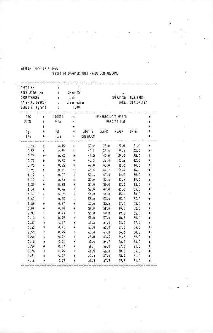
Univers
ity of
Cap
e Tow
n
AiRL!FT PUMP DATA SHEET result of DYNA MIC VOID RATIO COMPARISONS
- SHE ET No PIPE SIZE mm TESf/ THEORY MATER iAL DESC ! P £>ENS lfY kg i rn '' 3
GAS FLOW
Qg lis
0.24 0.55 G. 74 0.77 0.90 0.93 l \ •i '•L
1. 29 1.30 !. 34 1. 62 i .62 1. 8'1 2. 04 2. 08 2. 10 2.57 2. 62 2. '1'1 3. (H)
3. 03 3.54 .) . /0
3. '1! 4.16
LI!JU!D
Q! l / s
0.45 0.59 0.63 0. 72 0.65 i) , 71 0.67 0. 66 0.68 0. 76
0. 75 0.77 0. Ji)
o. 73 (} , 79 0. i7 n. 7i o. 79 ~) . ! f ,-, 7 i ~ .. ' . 0. 77 !) • 7'i i) , 77 !) , 77
36H !D both
c i ear wat er 1 (i(H)
OP ER ATOR : R.R.BERG DATE : 26/10/1987
DYNAMIC VO!D RATIO PREDICTiONS
G!OT • CLARK WEBER DATA CHI SHOLM
30.0 40 .0 44.5 4'j c;
47.0 46.0 50.6 53. 0 53.0 52.0 56.0 55. 0 57 .0 59 .0 59. 0 58. 0 61. 6 63 .0 63.4 63 .8 65.0 66 . 1 66 .5 67 .4 68 .2
23.0 34.0 40 .0 38 .4 43.0 42.7 47.4 50.6 50.0 qO Ii
54 . !) 53.i) 55.6 58 . 0 58.0 57.0 61 . 0 62. 0 63 . 0 63.3 64.7 66.0 66 .0 67.0 67.9
20 .0 29.0 34. 0 32 .6 36 .0 36 . 0 -'{l fl °t •J• v
42 .6 4·J (; 41 {;
45.0 45 .0 47. 0 49 . 0 49 .0 48. 5 52. 0 53 . 0 54.3 54.7 56 .0 57 . !) 58. 0 58.9 59.a
21. 0 33.0 38.0 4? {\ •• w
4(!, !)
46.0 48.0 49. 0 45.0 53. 0 48. !) \:' "T i\ J,) . '._i
55 .0 52. 0 55 .0 55 .0 57.0 54. 0 60. 0 59. !) 56 ,0 61. 0 63.0 61. 0 61. !)
t
t
=================================================================================

Univers
ity of
Cap
e Tow
n
AIRLIFT PUMP DATA SHEET result cf DYNAMIC YDID RATIO COMPARISONS
SHEET Ne P iPE Sl ZE :n:n TESTiTHEDRY MATERIAL DESCIP DENSITY ~gi:l''3
GAS * FLOlil *
Qg f.
l/s t
LIQUID FLDW
Q! li s
2 86mm ID both
clear water 1000
t
t
* * G!UT & f. CH!SHOUl
DYNAMIC
OPERATOR: R.P..BERG DATE: 27il0/!987
VOID RATiQ PREDICTIONS
CLARK l!EBER DATA
t
if
t
t
* ---------------------------------------------------------------------------------
2.88 +. 1.03 5:3. ·1 44. (l 34 .0 36 . 0 f.
4 ·17 ... , t 2. 16 , WU • 0 44.5 35.6 46. (! f.
6. 09 f. 3. 07 t 53.5 ii 7 (\ 1,.., 38. 4 44.0 * 7 .25 * 3.56 +. 54.0 48.3 39 .8 49.0 t
9 42 t 4. !4 • 55.7 52.0 42.6 49 0 • 10. 08 * 4.07 t 57.0 53.5 44.0 54. (! f.
i 2. i6 t 4.40 t 5·~.o 55. 9 46.2 56.5 t
!2.50 t 4 ~ ·j * "Q " ..!w..,J "" JJ, 7 46. 1 55.0 t
i4 . 45 f 4.62 • 60.6 58.3 48.6 62.2 t
!5. ·10 * 4. 74 f. 6!. 7 C"Q J,. 7 49.9 63. 0 * 17. 92 * 4.74 * 63. 0 6i. 6 51. 8 64. 7 * 18. 04 * 4. 99 f. 63.i) 6!. 0 5!. 4 64. 0 t
19 . '?5 f. 5.20 t 63.6 62.2 52.8 68. 0 f.
22. 43 f. 4.81 t 66.0 64.0 55.0 67.0 f.
=================================================================================

Univers
ity of
Cap
e Town
A!RL!FT PUMP DATA SHEET result of WEIGHT PRESSURE LOSS COM PARISON
------------------------------------------------------------------------------------------SHEET r~o
PIPE '.3IZE mm TEST/THEORY MATERIAL DESCIP DENS !TY kg I~" 3
- GAS
FLDW
Qg '1 i s
0.23%24 0.548378 0. 745737 0.76577
0.8%258 0. 934265
i.12068 1.292!8 1. 30936 1.34B87 1.62886 1.62961 1. 89'149 2.04163 2. 080i 1 2.1 01i6 2.57 732 2.62497 2. ·1·1372 3.0005
3.08782 3. 545! ! 3.7622! 3.91'12! 4.1649'1
f.
LIQUID FLOW
Ql lis
i}, 45 o. 5'1 0.63 0. 72 0.65 0. 71 0.67 0.66 0.68 0.76 0.69 0. 75 0.77 0.7
0.73 !) • 7'1 0. 77 0. 71
0.77 0. 71 0.77
0.77 0.77
both c i ear i1a t er
10!)0
f.
f.
DPEXATDR : X.R.9ERG DATE: 28/10/1987
WEiGHT PRESSURE LQSS in kP a
GIOT & CLARK & WEBER DATA i CHI SHOLM STE NNING
62 .38 5346 4'154 5127 47!! 4785 441 ! 4173 4!98 432! 3'10i 4020 3838 3607
3733 3425 3298 3267 3232 30'?8 3030
2913 2844
68.S4 5822 5351 5498 5056 5109 46a'i 4412 4430 4536 q (; ]j
4185
3724 3748 3833
336'1 3306 3275 "iS1 .) "\J ...
3059 ~llP
2939 2869
71 i1 6261 5888
5651 5688 535! 511 '1 5133 5216 4821 4915 4715 4'1'4 0
45!'i 4soJ
4263 4146 4074 4043 39i4 3806
3667 3584
70 47 5978
5177 5355 4820 4642 4553 4q{)'~
41 '17 4642 4i 'i7 41;1q
4286 4019 4019 3841 4108 3573 3662 3'130 3484 3306 3484 3484
• TOTAL ~ PRESSURE
LOSS kPa
7161 6259 6082 6082 6043 5984 5867 5886 5866
5778 c: ,-,7 7 ...:o .~ :
5680 5837 5689 5886 56!1 5788 5984 5582 5935 5544 5788 5886
==========================================================================================

Univers
ity of
Cape T
own
AIRLIFT PUMP DATA SHEE T result of WEIGHT PRESSURE LOSS COMPARISON
------------------------------------------------------------------------------------------SHEET No PIPE SlZE M
TEST/THEORY MATERIAL DESC ! P DENSJ TY kg im.'3
Bile; f.
FLDW f.
f.
Dn f. ~~
l i c * 2.88 f.
4.27 f.
6. 09 f
7.25 f
9. 42 f.
10. 08 p i6 f.
12. ~!o f.
14.45 1: .. 90 f
17. 92 f.
18.04 f.
19. 95 f
22. 43 f
LIQUID F L D ~
Qi l/s
j .03 ' 1 lb .... ~\ . 07 3.56 4. 14 4. 07 4.40 4.62 4.62 4. 74 4. 74 4. 99 5.20 4 Qj
86m" ID both
cl ear water 1000
f.
* f. G!OT t f. CHISHOLM
f. 6045 f 6862
6qc; 1 f. 6789
t.C.-i"i ....... _._. t 6324
* 6072 f 6i21 f. 579~3
f. 5637
* 5395 f. 5488 f. 5364 f 4974
OPERATOR: R.R.BERG DATE: 27il0/1987
WEIGHT PRESSURE I il '~r· ~~-·:>
1n kPa
CLAF:K & WEBER r"n t • .IHI,,
STENNJNG
8258 9718 9424 8i66 9480 7954 7751 9070 8248 7c;;; 8863 751:, 7081 8452 7396 68:!3 8255 6778 64'12 7916 641 i 6516 7931 6631 6i34 7573 5573 5930 737(1 545t. 5652 7090 5206 5728 7 { j.,{}
,j~, 5309 C'C''C' .;.;c..: 6986 4721 5! 7:, 6578 4i:l.l.t<
f.
f. TDTAL f. PRESSUF:E f. LUSS f kPa
f. 8838
* 8'.iQQ
f. 8221 f 7700 f. 7750 f. 7505 f. 7141 f 7044 f 7230 !- 6965 f. 7050 f. 6926 f 6995 !i: 6769
==========================================================================================

Univers
ity of
Cap
e Tow
n
========================================================================================== tl0£ 9£8Z 6£~(.
Lti~(
8£VZ 9ia t iQ\'(.
bvll \rOvZ l98i '"''I' ... '.ot .. J(.
l96l 0881 L£91 Z.1.L 1 t 9(1! it\ri 08vi £811 1)88 Zt.6 88:; ££L m 00£
~ , ~,
-o 'i
\.il~G
* * -i
*
* * * t
* i
t
* * lf
t
-!
lf
* :;.
t
* * * *
* * i
f
i
9Z££ GV££ %££ Z~O£
LLVZ U9Z: VL9l £li~ , r"!"' tt.:;L·l·
L68l l\rll lt9l 9L91 90tl L6ll t8il Z£0i 066 9L8 lBL !jti';''
.. ~ --¥ "f'"i
v9S vor 091
.. ~t:V J._1
:;ui 9!6i 6::'.91 Cd£i Bili 60£1 l\rU 8LOt .. r,. .. (~ ;'
666 £i6 198 968 lLL /''' Lt}L
BL9 LB£ l9£ ti:; £8\1 trzv ~ .-+, l · l !:
Z9l La 0£i
8£i t££ 99~
9E ~t. z.
Ei Lh vEZ Zl£ 6i~
rnz l9l 667.,
'tu.,
li'Z 69l \ill £1l ill 7"1""" 1 .... LG
tt:r LE vll Lirl (..t:
.,.,,...,,.
.~jtijf!l
~CL
869 OOL 9~9
6\:£ Z6£ t.09 86t (..f::i
B6v m vzv L:;v 60t t· ·t~
rJLL
Vl£ :} i i,
£6Z lOC
9£(. 9E El £81 Lb
* i
*
t
i
i
i
i
t
i
i
*
* i
i
i
i
* t
031~IOOW WlOHSIHJ ' lH~lJ 9NINN31S I
i
r'I ' " ''" C 1j /1 U ~ * SSOl 3HGSS38d NGliJi~:i i
oo ·ooor LB611011sz: :31ua lCfCl-t ..t~a!J
8838·~·~ :H01ij83d0 4~cq
GI wu:9£ (!0 . t
LL ·o LL 'O t•L \)
LL'O lL ·o LL ' O f.,£ ·o 1L'O LL"O 6L'O ~L "O OL 'O LL 'O ~L \ i b9'0 9L'O 89'(i '1'1 {}
L9'0 lL 'O £9'(! lL'O £9'0 6C.'(i
;1i ' (i
S/ t
rn
fi\01.:i GiflOil
* * i
i
* * t
* * i
;;
;;
* ;;
* i
f
it
;;
t
* i
if
i
t
* ' * ~
9i ·v l6"£ 9L'£ ~~·l
t ·{} ~
t}t} l.
t •t • L ,,, ·~ L'i .::_,
8£ 'l 01 ·z b i} (..
vo·z 06 • r £9. t £9't ~£ 'l 1~ · t 6Z. t ll 'l £6'0 06 ' (i LL U
£i'O r~· · =~ v tl'O
Sf! 55
MOl:l S98
~ vW/ 5~i .i:l!SN3G dIJS3U ltfI~3iQW
A~G3H1/1S3 1
Uill! 3ZI~; 3did ,., ~· ' ............ Vf~ l:lj ti ~c
NOSIH~dWOJ SSOl 3~n SS3~d NGilJI~~ fD l1nsa1 133HS ijl~G dWGd l~Il~Jij

Univers
ity of
Cap
e Tow
n
AIRLIFT PUMP DATA SHEET result of WEIGHT PRESSURE LOSS COMPARISON
SHEET No PIPE SIZE mm TEST/THEORY MATERIAL DESC!P DENS !TY kg i m'' 3
GAS f.
FLDW f.
f.
Qg f.
lis f.
''!in ~· ....... lf 4 .-,.,
f. "t.t.f
6. 09 f.
7. 25 * 'i 42 f.
10.08 f.
p !6 ~
12. 50 f.
14.45 f.
15. 90 f.
17.n f.
!8. 04 19 95 f
22.43 *
LIQUID FLOW
(1\ wt
li s
t {°} ~
·j i6 ... 3. 07 3.56 4, 14 4. 07 4. 40 4.62 4.62 4. 74 4.74 4. 99 5.20 4.8!
2. 00
both OPERATOR: R.R.BERS clear water DATE: 27/10/1987
1000.00
• FRICTION PRESSURE ; ,;,-,,, .... ~L!J~
t in kPa
• t STENiWJG CLARK & CHISHOLM MODIFIED
WEBER CLARK
6045 8258 9718 '1424 f. 6862 8166 9480 7954
685! 7751 '1070 8248 f 6789 7533 8863 7'" ~ ,.,J_l ._\
• 6523 7081 3452 73'16 f 6324 6853 8255 6778
60 72 64'12 7916 6411 6121 65!6 7931 6631
f. 57'18 6134 7573 5573 f 5637 593(1 737(1 5456
• 5395 5652 7090 5206 f 5488 5728 7!60 5309 t 5364 5565 6'i86 .'f ·jj
"t .......
f. 4974 5175 6578 4868
' f
f.
f. DATA f. kPa
• Q::l7~ {\ {\ ........ .J ..... ... ....
f. 8289.00 f. 822!. 00
• 7700. 00 t 7750.00
• 7505.00 f. 7141 . 00 t 7044 .00 f 7230. (H)
f. 6965.00
• 7050.00
• 6926.00 f 6'?95. 00 t 676'?.00
==========================================================================================

Univers
ity of
Cap
e Tow
n
APPENDIX D
EXAMINATIONS WRITTEN BY THE AlJI'HOR TO CXMPLETE
THE REQUIREMENTS OF THE DEGREE

Univers
ity of
Cap
e Tow
n
Examination
CIV 540Z
CIV 536Z
CIV 516Z
SBA 200F
CIV 542Z
mESIS
\ 8 JUL \989
APPENDIX D
Finite Element Analysis
Coastal Engineering Practice
Coastal Hydraulics
Fhysical Oceanograpiy
Irrigation Systems
"Hydro-:piet1DB.tic conveying of liquid
by means of an airlift pt.mp"
Total
Credit requirements for degree = 40
Credit Ratir!B
4
5
5
5
3
42