Hybrid Thermo-Mechanical Contact Algorithm for 3D SPH-FEM

275

IV International Conference on Particle-Based Methods - Fundamentals and ApplicationsPARTICLES 2015

E. Oñate, M. Bischoff, D.R.J. Owen, P. Wriggers & T. Zohdi (Eds)

Hybrid Thermo-Mechanical Contact Algorithm for 3D SPH-FEM Multi-Physics Simulations

Kirk A. Fraser1,2*, Lyne St-Georges2, Laszlo I. Kiss2 and Yves Chiricota2

1 Aluminium Research Centre-REGAL2 Université du Québec à Chicoutimi (UQAC)

555, boulevard de l’UniversitéSaguenay (Québec) G7H 2B1 * e-mail: [email protected]

Key words: Thermo-mechanical contact, smoothed particle hydrodynamics, computational plasticity, solid mechanics, friction stir welding, high speed machining, forging, extrusion

Abstract: Numerical simulation of complex industrial processes has become increasingly common in recent years. Depending on the nature of the industrial application, multiple types of physical phenomena may need to be considered as well as the interaction of multiple disjoint bodies. This paper is focused on industrial applications with large plastic deformation. Such processes are typically not well treated by finite element (FE) methods. For this reason, the smoothed particle hydrodynamics method (SPH) is used. In this work, we introduce a robust and straightforward thermo-mechanical contact algorithm for multi-physics SPH simulations in 3D.

1. INTRODUCTIONMulti-physics simulations more often than not include the interaction of multiple bodies. For

example, in a ballistics impact analysis, the projectile is considered as a distinct body and the object to be impacted is another. The interaction between these two bodies is a large area of research. A contact algorithm is needed to prevent the elements of one body from penetrating into those in the other body. The type of contact algorithm to be used depends strongly on the simulation approach. For highly non-linear transient problems, typically an explicit time stepping tactic is used. In such a case penalty contact methods provide an efficient and robust means to transfer forces from one body to another. One of the earlier implementation was by Hughes et al. [1].

In the smoothed particle hydrodynamics (SPH) method, contact between bodies has been enforced by many different approaches. One of the simpler approaches is to allow the two bodies to interact directly through the SPH equations. This has certain qualities, however, the biggest drawback is that the elements at the interface of the two bodies will impart shear stresses that will cause a “no-slip” behavior. For industrial processes like friction stir welding (FSW) and high speed machining (HSM), the “no-slip” boundary condition cannot easily be implemented. A very high SPH element density is needed in the contact region to correctly resolve the shear stresses due to this type of boundary condition. For such industrial processes, a friction based contact model is often adopted with little to no loss of coherency.

Throughout SPH literature, very little has been presented in terms of a node to surface

Hybrid thermo-mechanical contact algorithm for 3D SPH-FEM multi-physics simulations

276

Kirk A. Fraser, Lyne St-Georges, Laszlo I. Kiss and Yves Chiricota

2

penalty contact method with friction. Node to node contact models on the other hand have been reasonably well documented. Of the models that have been published, the Belytschko [2, 3] pinball method is rather popular and requires very little modification to be applied to SPH. Vignjevic and Campbell [4] discuss three penalty based contact models and compare the results of the impact of two blocks in 2D. They note that all the methods that they investigate suffer from an instability at the corners of the SPH body. Seo et al. [5, 6] present a rigorous treatment of SPH contact for axisymmetric problems. Wang et al. [7] provide a succinct treatment of a general contact algorithm with friction between a flexible SPH body and either a flexible or rigid body. They present their formulation in 2D and mention that only minor changes are needed to move to 3D. We have found on the other hand that a number of modifications are indeed needed in 3D.

Many commercial simulation codes such as LS-DYNA, Abacus, Hyperworks, etc. provide a means to couple SPH and finite element (FE) bodies mechanically. However, to our knowledge, a robust thermo-mechanical contact algorithm has not yet been presented nor implemented in any presently available multi-physics SPH codes.

In this paper, we outline the implementation of a thermo-mechanical penalty contact algorithm that can be used for SPH-SPH or SPH-FE simulations. The implementation that we will present supposes that the SPH body is flexible, while the FE body is reasonably approximated as rigid. Some minor changes would be needed to extend the algorithm to account for a deformable SPH body with either another deformable SPH body or FE body. The code is written using CUDA Fortran, this allows us to use a fine grained parallel implementation of the SPH code on the graphics processing unit (GPU). At the end of the paper, we present a validation case for the algorithm using a high speed machining example. The underlying physics show close parallels to other industrial processes such as friction stir welding, extrusion and forging and as such we expect the algorithm to be useful for these processes as well. 2. THE SPH METHOD

A brief overview of the SPH implementation used for this work is presented here. Most of the details are glazed over since the focus of the paper is the contact algorithm. The conservation of mass for a temporally changing compressible system is: 𝑑𝑑𝑑𝑑𝑑𝑑𝑑𝑑 + ∇ ∙ 𝑑𝑑�̅�𝑣 = 0 ( 1 )

𝑑𝑑 is the material point density, �̅�𝑣 is the velocity and 𝑑𝑑 is time. We can write the discrete SPH equation for conservation of mass:

𝑑𝑑𝑑𝑑𝑖𝑖𝑑𝑑𝑑𝑑 = ∑𝑚𝑚𝑗𝑗(𝑣𝑣𝑖𝑖𝛽𝛽 − 𝑣𝑣𝑗𝑗𝛽𝛽)

∂𝑊𝑊𝑖𝑖𝑗𝑗∂𝑥𝑥𝑖𝑖𝛽𝛽

𝑁𝑁𝑖𝑖

𝑗𝑗=1 ( 2 )

𝑁𝑁𝑖𝑖 is the number of neighbors of the ith particle, 𝑚𝑚𝑗𝑗 is the mass of the jth particle and ∂𝑊𝑊𝑖𝑖𝑗𝑗 ∂𝑥𝑥𝑖𝑖𝛽𝛽⁄ is the gradient of the smoothing function (see Liu and Liu [8] for more details). Conservation of momentum for a continuum is given by:

277


3

𝑑𝑑�̅�𝑣𝑑𝑑𝑑𝑑 = 1

𝜌𝜌 ∇ ∙ �̿�𝜎 + �̅�𝑔 + 1𝑚𝑚 �̅�𝐹𝑐𝑐𝑐𝑐𝑐𝑐𝑐𝑐𝑐𝑐𝑐𝑐𝑐𝑐 ( 3 )

�̿�𝜎 is the Cauchy stress tensor (total stress), �̅�𝑔 is the gravity vector and �̅�𝐹𝑐𝑐𝑐𝑐𝑐𝑐𝑐𝑐𝑐𝑐𝑐𝑐𝑐𝑐 is the contact force vector that is found from the contact algorithm (to be explained latter). The SPH equation is then:

𝑑𝑑𝑣𝑣𝑖𝑖𝛼𝛼𝑑𝑑𝑑𝑑 = ∑𝑚𝑚𝑗𝑗 (

𝜎𝜎𝑖𝑖𝛼𝛼𝛼𝛼𝜌𝜌𝑖𝑖2

+𝜎𝜎𝑗𝑗𝛼𝛼𝛼𝛼𝜌𝜌𝑗𝑗2

)∂𝑊𝑊𝑖𝑖𝑗𝑗∂𝑥𝑥𝑖𝑖𝛼𝛼

𝑁𝑁𝑖𝑖

𝑗𝑗=1+ 𝑔𝑔𝑖𝑖𝛼𝛼 + 1

𝑚𝑚𝑖𝑖𝐹𝐹𝑐𝑐𝑐𝑐𝑐𝑐𝑐𝑐𝑐𝑐𝑐𝑐𝑐𝑐𝑖𝑖

𝛼𝛼 ( 4 )

This is known as the symmetric form of the momentum equation. For many industrial processes, including the effects of heat transfer is of key importance. We seek to provide a discrete SPH equation for the heat diffusion equation: 𝜕𝜕𝜕𝜕𝜕𝜕𝑑𝑑 = 1

𝜌𝜌𝐶𝐶𝑝𝑝(𝑘𝑘∇2𝜕𝜕 + �̇�𝑞) ( 5 )

𝜕𝜕 is the material point temperature, 𝐶𝐶𝑝𝑝 is the specific heat capacity, 𝑘𝑘 is the thermal conductivity and �̇�𝑞 takes into account heat generation due to plastic deformation or friction work. We have found that Jubelgas’s [9] SPH formulation for heat transfer works well and is used in this work:

𝑑𝑑𝜕𝜕𝑖𝑖𝑑𝑑𝑑𝑑 = 1

𝜌𝜌𝑖𝑖𝐶𝐶𝑝𝑝𝑖𝑖[∑

𝑚𝑚𝑗𝑗𝜌𝜌𝑗𝑗

(4𝑘𝑘𝑖𝑖𝑘𝑘𝑗𝑗)(𝑘𝑘𝑖𝑖 + 𝑘𝑘𝑗𝑗)

(𝜕𝜕𝑖𝑖 − 𝜕𝜕𝑗𝑗)|𝑥𝑥𝑖𝑖𝑗𝑗|

2 𝑥𝑥𝑖𝑖𝑗𝑗∂𝑊𝑊𝑖𝑖𝑗𝑗∂𝑥𝑥𝑖𝑖𝛼𝛼

+ �̇�𝑞𝑁𝑁𝑖𝑖

𝑗𝑗=1] ( 6 )

This form uses the harmonic mean for the thermal conductivity and has been shown to provide good results for materials with large variations of thermal conductivity. Strain rates, deviatoric stresses, the spin tensor and objective stress updates are calculated according to the common approach; further details can be found in any SPH publication that treats strength of materials [10-20]. We use a semi-implicit (modified Euler, similar to Cleary et al. [11]) integration scheme that is well suited for solid mechanics problems with SPH. The plasticity algorithm is a standard Johnson-Cook model with the radial-return approach. We also use a novel adaptive neighbor searching algorithm that is described by Fraser [14]. The smoothing function we use in this work is the hyperbolic spline recently developed by Yang et al. [21]. We have found this kernel to be a nice compromise between the good performance of Monaghan’s cubic spline for disordered SPH elements and the improved behavior of Johnson’s quadratic function for impact problems with strong compression.

3. THE THERMO-MECHANICAL CONTACT ALGORITHM

The remaining portion of the paper is now focused on finding the value of 𝐹𝐹𝑐𝑐𝑐𝑐𝑐𝑐𝑐𝑐𝑐𝑐𝑐𝑐𝑐𝑐𝑖𝑖𝛼𝛼 and

the transfer of thermal energy. A contact example is shown on the left side of Figure 1. Here, a flexible body with an initial velocity is meshed with SPH elements (red part), a rigid surface (grey part) is meshed with finite elements. The general layout for the contact between the SPH and finite elements is shown in the right side of Figure 1. The ih SPH element has a center at

278


4

�̅�𝑥𝑖𝑖. The jth triangular element has vertices A, B and C with positions; �̅�𝑥𝐴𝐴𝑗𝑗, �̅�𝑥𝐵𝐵𝑗𝑗 and �̅�𝑥𝐶𝐶𝑗𝑗 respectively. The triangular element has a surface normal vector that is �̂�𝑛𝐹𝐹𝐹𝐹𝐹𝐹𝑗𝑗 . The normal vector is found from:

�̂�𝑛𝐹𝐹𝐹𝐹𝐹𝐹𝑗𝑗 =�̅�𝑈𝑗𝑗x�̅�𝑉𝑗𝑗‖�̅�𝑈𝑗𝑗x�̅�𝑉𝑗𝑗‖

( 7 )

�̅�𝑈𝑗𝑗 = �̅�𝑥𝐵𝐵𝑗𝑗 − �̅�𝑥𝐴𝐴𝑗𝑗 and �̅�𝑉𝑗𝑗 = �̅�𝑥𝐶𝐶𝑗𝑗 − �̅�𝑥𝐴𝐴𝑗𝑗 , the ‖ ‖ signifies the magnitude of the vector and the ̂ represents a normalized unit vector.

Figure 1 – Node to Surface Contact

In order to take advantage of the efficiency of the uniform grid neighbor search (also called bucket search, see Fraser [14] for details of our implementation), a sphere is embedded at the centroid of each of the triangular finite elements. The radius of the sphere is chosen so that all of the nodes of the element are enclosed within the sphere. In this manner, the neighbor search is performed not only over the SPH domain, but also over the embedded spheres in the finite elements. This allows us to form a list of potential contact pairs between the SPH body and the FE body. 3.1 CONTACT DETECTION The next step is to determine which of the potential pairs are contact pairs. Our approach is similar to the algorithm described by Ericson [22]. We have made some slight modification in order account for the movement of the SPH and the FE body. This is done by taking into account

279


5

the relative velocity, �̅�𝑣𝑅𝑅𝑅𝑅𝑅𝑅 = �̅�𝑣𝑖𝑖 − �̅�𝑣𝑗𝑗, between an SPH element with velocity �̅�𝑣𝑖𝑖, and a finite element node with velocity �̅�𝑣𝑗𝑗. as shown in Figure 2. We perform a check to ensure that the SPH and finite elements are approaching each other (impending contact). This is done by ensuring that the penetration rate, �̇�𝛿 = −(�̂�𝑛𝐹𝐹𝐹𝐹𝐹𝐹𝑗𝑗 ∙ �̅�𝑣𝑅𝑅𝑅𝑅𝑅𝑅), is greater than zero. If this is less than or equal to zero, the pair are moving away and are not considered to be contact candidates. Next, we test to see if the contact point, �̅�𝑄𝑗𝑗 lies within the bounds of the triangular element. This is done by performing what is called the “inside-outside” check:

[(�̅�𝑥𝐵𝐵𝑗𝑗 − �̅�𝑥𝐴𝐴𝑗𝑗) × (�̅�𝑄𝑗𝑗 − �̅�𝑥𝐴𝐴𝑗𝑗)] ∙ �̂�𝑛𝐹𝐹𝐹𝐹𝐹𝐹𝑗𝑗 ≥ 0 𝑎𝑎𝑛𝑛𝑎𝑎

[(�̅�𝑥𝐶𝐶𝑗𝑗 − �̅�𝑥𝐵𝐵𝑗𝑗) × (�̅�𝑄𝑗𝑗 − �̅�𝑥𝐵𝐵𝑗𝑗)] ∙ �̂�𝑛𝐹𝐹𝐹𝐹𝐹𝐹𝑗𝑗 ≥ 0 𝑎𝑎𝑛𝑛𝑎𝑎

[(�̅�𝑥𝐴𝐴𝑗𝑗 − �̅�𝑥𝐶𝐶𝑗𝑗) × (�̅�𝑄𝑗𝑗 − �̅�𝑥𝐶𝐶𝑗𝑗)] ∙ �̂�𝑛𝐹𝐹𝐹𝐹𝐹𝐹𝑗𝑗 ≥ 0

( 8 )

All of the above relations must hold for the contact point to be within the triangle. �̅�𝑥𝐴𝐴𝑗𝑗 is the position vector for the Ath node on the triangular element. The right hand rule is respected for finding the normal of the element. The greater than or equal to ensures that a contact point on the edge of the triangle is considered to be within bounds.

Figure 2 – Relative velocity diagram

Once a contact point that lies within the triangle is found, we calculate the penetration depth, 𝛿𝛿, from

𝛿𝛿 = 12

ℎ𝑖𝑖𝑆𝑆𝑆𝑆𝑆𝑆𝑆𝑆 − |�̂�𝑛𝐹𝐹𝐹𝐹𝐹𝐹𝑗𝑗 ∙ (�̅�𝑥𝑖𝑖 − �̅�𝑥𝐴𝐴𝑗𝑗) | ( 9 )

280


6

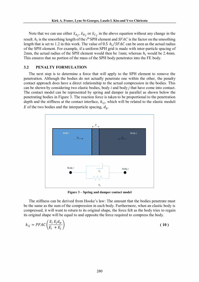
Note that we can use either �̅�𝑥𝐴𝐴𝑗𝑗 , �̅�𝑥𝐵𝐵𝑗𝑗 or �̅�𝑥𝐶𝐶𝑗𝑗 in the above equation without any change in the result. ℎ𝑖𝑖 is the smoothing length of the ith SPH element and SFAC is the factor on the smoothing length that is set to 1.2 in this work. The value of 0.5 ℎ𝑖𝑖 𝑆𝑆𝑆𝑆𝑆𝑆𝑆𝑆⁄ can be seen as the actual radius of the SPH element. For example, if a uniform SPH grid is made with inter-particle spacing of 2mm, the actual radius of the SPH element would then be 1mm; whereas ℎ𝑖𝑖 would be 2.4mm. This ensures that no portion of the mass of the SPH body penetrates into the FE body. 3.2 PENALTY FORMULATION The next step is to determine a force that will apply to the SPH element to remove the penetration. Although the bodies do not actually penetrate one within the other, the penalty contact approach does have a direct relationship to the actual compression in the bodies. This can be shown by considering two elastic bodies, body i and body j that have come into contact. The contact model can be represented by spring and damper in parallel as shown below the penetrating bodies in Figure 3. The reaction force is taken to be proportional to the penetration depth and the stiffness at the contact interface, 𝑘𝑘𝑖𝑖𝑗𝑗, which will be related to the elastic moduli 𝐸𝐸 of the two bodies and the interparticle spacing, 𝑑𝑑𝑝𝑝.

Figure 3 – Spring and damper contact model

The stiffness can be derived from Hooke’s law: The amount that the bodies penetrate must be the same as the sum of the compression in each body. Furthermore, when an elastic body is compressed, it will want to return to its original shape, the force felt as the body tries to regain its original shape will be equal to and opposite the force required to compress the body.

𝑘𝑘𝑖𝑖𝑗𝑗 = 𝑃𝑃𝑆𝑆𝑆𝑆𝑆𝑆 (𝐸𝐸𝑖𝑖 𝐸𝐸𝑗𝑗𝑑𝑑𝑝𝑝𝐸𝐸𝑖𝑖 + 𝐸𝐸𝑗𝑗 ) ( 10 )

281


7

The penalty factor is needed to allow the stiffness to be easily adjusted for different simulations. 𝑃𝑃𝑃𝑃𝑃𝑃𝑃𝑃 is typically set to 1.0, but can be set to lower values in the case of high velocity impact. Contact damping, 𝑃𝑃𝑖𝑖𝑖𝑖, is included to damp out oscillations in the contact behavior along the element unit normal direction. The damping is proportional to the relative velocity of the contacting bodies. The value of the damping factor is found from:

𝑃𝑃𝑖𝑖𝑖𝑖 = 𝐷𝐷𝑃𝑃𝑃𝑃𝑃𝑃 [(𝑚𝑚𝑖𝑖 + 𝑚𝑚𝑖𝑖)√𝑘𝑘𝑖𝑖𝑖𝑖 (𝑚𝑚𝑖𝑖 + 𝑚𝑚𝑖𝑖𝑚𝑚𝑖𝑖𝑚𝑚𝑖𝑖

)] ( 11 )

Again, a factor is used to provide a damping that can be a fraction of the critical damping. If 𝐷𝐷𝑃𝑃𝑃𝑃𝑃𝑃 is set to 1.0, critical damping is obtained. This damping approach here is similar to the method used in LS-DYNA [23]. The contact force vector, �̅�𝑃𝑁𝑁𝑁𝑁𝑁𝑁𝑁𝑁𝑁𝑁𝑁𝑁, along the normal direction is then:

�̅�𝑃𝑁𝑁𝑁𝑁𝑁𝑁𝑁𝑁𝑁𝑁𝑁𝑁 = (𝑘𝑘𝑖𝑖𝑖𝑖𝛿𝛿 − 𝑃𝑃𝑖𝑖𝑖𝑖�̇�𝛿) �̂�𝑛𝐹𝐹𝐹𝐹𝐹𝐹𝑖𝑖 ( 12 )

3.3 FRICTION FORMULATION We use a sliding friction model that is commonly referred to as Coulomb friction. In this model, a force is applied to the SPH element that is opposite to the relative motion of travel. Consider the situation where body i is moving with velocity �̅�𝑣𝑖𝑖 and body j is moving with velocity �̅�𝑣𝑖𝑖, then the relative direction of travel will be along �̅�𝑣𝑅𝑅𝑅𝑅𝑁𝑁 = �̅�𝑣𝑖𝑖 − �̅�𝑣𝑖𝑖. The friction force, �̅�𝑃𝐹𝐹𝑁𝑁𝑖𝑖𝐹𝐹𝐹𝐹𝑖𝑖𝑁𝑁𝐹𝐹, is:

�̅�𝑃𝐹𝐹𝑁𝑁𝑖𝑖𝐹𝐹𝐹𝐹𝑖𝑖𝑁𝑁𝐹𝐹 = 𝜇𝜇(𝜎𝜎𝑦𝑦,𝑇𝑇) �̅�𝑃𝑁𝑁𝑁𝑁𝑁𝑁𝑁𝑁𝑁𝑁𝑁𝑁(−�̂�𝑛𝑇𝑇) ( 13 )

𝜇𝜇(𝜎𝜎𝑦𝑦,𝑇𝑇) is the coefficient of friction that can be a function of the yield stress of the material and the temperature. �̂�𝑛𝑇𝑇 is a normalized unit vector in the direction of relative motion. Although tangential damping can be added to the friction force, we do not include this in the current work. The tangential relative velocity is found by decomposing the relative velocity vector into its normal and tangential components:

�̅�𝑣𝑅𝑅𝑅𝑅𝑁𝑁𝑇𝑇 = �̅�𝑣𝑅𝑅𝑅𝑅𝑁𝑁 − �̅�𝑣𝑁𝑁𝑁𝑁𝑁𝑁𝑁𝑁

�̅�𝑣𝑁𝑁𝑁𝑁𝑁𝑁𝑁𝑁 = 𝛿𝛿 ̇ �̂�𝑛𝐹𝐹𝐹𝐹𝐹𝐹𝑖𝑖 ( 14 )

Once we have the relative tangential velocity, we can easily find the unit normalized tangential vector from:

�̂�𝑛𝑇𝑇 =�̅�𝑣𝑅𝑅𝑅𝑅𝑁𝑁𝑇𝑇‖�̅�𝑣𝑅𝑅𝑅𝑅𝑁𝑁𝑇𝑇‖

( 15 )

3.4 CONTACT FORCE

The penetration resisting force (in the surface normal direction, �̅�𝑃𝑁𝑁𝑁𝑁𝑁𝑁𝑁𝑁𝑁𝑁𝑁𝑁) and the friction force (�̅�𝑃𝐹𝐹𝑁𝑁𝑖𝑖𝐹𝐹𝐹𝐹𝑖𝑖𝑁𝑁𝐹𝐹) have to be combined together to give the total contact interface force, �̅�𝑃𝐶𝐶𝑁𝑁𝐹𝐹𝐹𝐹𝑁𝑁𝐹𝐹𝐹𝐹:

282


8

�̅�𝐹𝐶𝐶𝐶𝐶𝐶𝐶𝐶𝐶𝐶𝐶𝐶𝐶𝐶𝐶 = �̅�𝐹𝑁𝑁𝐶𝐶𝑁𝑁𝑁𝑁𝐶𝐶𝑁𝑁 + �̅�𝐹𝐹𝐹𝑁𝑁𝐹𝐹𝐶𝐶𝐶𝐶𝐹𝐹𝐶𝐶𝐶𝐶 ( 16 )

In the explicit SPH code, the forces are combined to impose an acceleration that is included when performing the time integration. The total acceleration due to contact is:

𝑑𝑑𝑣𝑣𝐹𝐹𝛼𝛼𝑑𝑑𝑑𝑑 |

𝐶𝐶𝐶𝐶𝐶𝐶𝐶𝐶𝐶𝐶𝐶𝐶𝐶𝐶= 1𝑚𝑚𝐹𝐹

𝐹𝐹𝐶𝐶𝐶𝐶𝐶𝐶𝐶𝐶𝐶𝐶𝐶𝐶𝐶𝐶𝐹𝐹𝛼𝛼

= 1𝑚𝑚𝐹𝐹

(𝐹𝐹𝑁𝑁𝐶𝐶𝑁𝑁𝑁𝑁𝐶𝐶𝑁𝑁𝐹𝐹𝛼𝛼 + 𝐹𝐹𝐹𝐹𝑁𝑁𝐹𝐹𝐶𝐶𝐶𝐶𝐹𝐹𝐶𝐶𝐶𝐶𝐹𝐹

𝛼𝛼) ( 17 )

3.5 THERMAL CONTACT A reasonable approximation of thermal contact can be attained by assuming no contact resistance (perfect thermal contact). To this end, the SPH heat diffusion equation can be used to include thermal contact. The key to including thermal contact is to provide separate neighbors lists for the mechanical part and the thermal part. In this work, we have used four different lists:

1. NeibMech - This is a list that contains the neighbors only within the deformable parts

2. NeibTherm - This is a list that contains the neighbors for the thermal problem 3. NeibCont - This is a list that contains the neighbors for the potential contact pairs 4. NeibContTherm - This is a list that contains the neighbors for the potential contact pairs

to distribute the heat generated due to friction work

A bit of extra work is needed to build the individual lists; however the overhead is not significant as long as the lists are built within the same subroutine. The crucial concept in this sense is that we only perform the bucket search once for each particle to form the four individual lists. Imagine a two body collision problem with non-collinear approaching velocities (upon impact a certain amount of sliding will occur), where one body is at 500°C and the other body is at 20°C. Body #1 is made of aluminum and is very soft at 500°C. We expect the body to be subject to large deformation, as such, body #1 is modeled with SPH elements. We will assume that body #2 is rigid (steel) and can be modeled by creating a contact surface with zero thickness triangular plate elements. Upon impact we want to be able to treat the mechanical contact along with friction as well as the transfer of thermal energy from one body to the other. In this example, the lists will contain the following elements:

1. NeibMech - All SPH elements from body #1 (with self-interaction) 2. NeibTherm - All SPH elements from body #1 and 2 (both with self-interaction) 3. NeibCont - Body #1 with the spheres imbedded in the triangular FE mesh 4. NeibContTherm - Body #2 (no self-interaction) with body #1 (no self-interaction)

By creating different neighbor lists, the conservation of mass and momentum equations are evaluated using NeibMech for body #1 only. The heat transfer equation (includes the thermal contact) will be evaluated using NeibTherm for body #1 and 2. The mechanical contact is evaluated by finding actual contact pairs within the NeibCont list. And finally, heat is divided between the two interfaces during friction heat generation using NeibContTherm. Again, it is important to remember that this thermal contact model is representative of perfect thermal contact. We could account for contact resistance, convection and radiation at the contact

283


9

interface using a source term in the SPH heat equation. The method will become clearer following the HSM example in the next section. 4. HIGH SPEED MACHINING EXAMPLE The HSM example is set up according to the work of Villumsen and Fauerholdt [24] and Limido et al. [25]. In their work, they employ an adiabatic SPH approach. In our implementation we will investigate the chip formation including the effect of heat generation due to plastic deformation and friction work. Furthermore, heat will be allowed to transfer not only within the aluminum work piece (WP) but also to the cutting tool. The model setup is as explained in [24], all parameters are kept the same except the value of C in the Johnson-Cook model is zero in our work. We argue that the effect of strain rate should not be included in a velocity scaled model (they use a factor of 5 as do we here). Also, we have not put a limit on the effective plastic strain (Villumsen used a limit of 1.2). We found that doing so provides a significant underestimation of the cutting forces. Figure 4 shows the AL 6082-T6 WP and the cutting tool (CT). Notice that the tool SPH elements do not belong to the NeibMech list. Both the SPH elements on the WP and the CT are included in the NeibTherm list. The zero thickness triangular finite elements that define the contact surface of the tool can also be seen. The WP and the CT interact mechanically through the NeibCont list (not shown in figure), the heat transfer back and forth between the WP and the CT occurs through the SPH heat transfer kernel using the NeibTherm list. In a friction heating model, the heat generated at the interface must be split according to the ratio of thermal material properties of the two bodies. This is done through the NeibContTherm list.

Figure 4 – Cutting Model

The results of the stress and temperature distribution when the tool has cut 1.75mm into the work piece can be seen in Figure 5. We note that the chip formation is very similar to that obtained in [24]. The high stress zone in the simulation model correlates very well with what we have seen in the literature. This stress distribution cannot be reproduced with a mesh based

284


10

method such as the finite element method. A number of authors have reported on the importance of including the temperature rise during the cutting process. Abukhshim at al. [26] report that the cutting temperature can range between 150°C to over 400°C depending on the cutting parameters. We have found a maximum interface temperature (averaged over the cutting simulation) of 376°C. This is well within the reported range from [26]. Other authors [27-29] have investigated the cutting temperature, they typically report temperatures in the range of 0.25 - 0.7 of the melting temperature of the metal. We expect the interface temperatures to be higher for AL 6082-T6 compared to AL 6061-T6 since it is a higher strength alloy.

Figure 5 – Stress and temperature results (tool position: 1.75mm)

We are now in a position to show that the effect of temperature in a high speed cutting model is significant and should not be ignored. We have run the same model with heat transfer and heat generation (w HT) and without (wo HT). The decrease in normal cutting force is significant when the heat generation due to plastic deformation and friction work is included. The thickness of the chip increases slightly with heat transfer. This then leads to a slight increase in tangential force.

Figure 6 – Cutting force results (average cutting force)

285


11

Using a friction coefficient of 0.2 and no heat transfer provides an overestimate on the normal cutting forces by 12.5%. When we take into account heat generation effects, the normal cutting force drops and provides a slight underestimate by 3.9%. The tangential cutting forces are strongly influenced by the value of the coefficient of friction chosen. We have used 0.2 since this was the value used in [24]. However, the exact value for the tangential force can easily be obtained in the model by tuning the coefficient of friction. A comparison of the cutting forces is shown in Figure 6. The experimental cutting forces are taken from [24]. The mesh density used in our work is 125,000 SPH elements per cm3, this density provides high enough resolution to predict the cutting forces. However, this density is not fine enough to reproduce the shear band pattern. Villumsen used 512,000 elements/cm3 in order to show this phenomenon. 5. CONLUSIONS In this paper we have outlined a straightforward and robust approach to simulate 3D multi-physics problems with thermo-mechanical contact. The algorithm presented uses a penalty mechanical contact algorithm by using a node to surface approach. The deformable SPH body is checked for contact against a rigid zero thickness triangular plate element mesh. The thermal contact is carried out through the SPH heat diffusion kernel, which provides a thermal contact interface with no losses. In the future, we plan to work towards extending the algorithm to include a thermal contact resistance. This could be done by introducing a heat loss term in the heat diffusion equation for the elements at the interface of the contacting bodies. In this work, we have shown the accuracy of the proposed thermo-mechanical contact algorithm through a high speed machining example. The cutting forces found using our algorithm are very close to the forces obtained experimentally. 6. ACKNOWLEDGEMENTS The authors would like to acknowledge the financial support of CQRDA, FQRNT and GRIPS. A part of the research presented in this paper was financed by the Fonds de recherche du Québec - Nature et technologies by the intermediary of the Aluminium Research Centre REGAL. Also, we are grateful to NVIDIA for providing the GPU used for the simulations and to PGI for providing the license for the CUDA Fortran Compiler. REFERENCES [1] Hughes TJR, Taylor RL, Sackman JL, Curnier A, Kanoknukulchai W. A finite element method for a class of contact-impact problems. Computer Methods in Applied Mechanics and Engineering. 1976;8:249-76. [2] Belytschko T, Lin JI. A three-dimensional impact-penetration algorithm with erosion. International Journal of Impact Engineering. 1987;5:111-27. [3] Belytschko T, Yeh IS. The splitting pinball method for contact-impact problems. Computer Methods in Applied Mechanics and Engineering. 1993;105:375-93. [4] Vignjevic R, Campbell J. A penalty approach for contact in smoothed particle hydrodynamics. International Journal of Impact Engineering. 1999;23:945-56. [5] Seo S, Min O. Axisymmetric SPH simulation of elasto-plastic contact in the low velocity impact. Computer Physics Communications. 2006;175:583-603. [6] Seo S, Min O, Lee J. Application of an improved contact algorithm for penetration analysis in SPH.

286


12

International Journal of Impact Engineering. 2008;35:578-88. [7] Wang J, Wu H, Gu C, Hua H. Simulating frictional contact in smoothed particle hydrodynamics. Science China - Technological Sciences. 2013;56:1779-89. [8] Liu GR, Liu MB. Smoothed particle hydrodynamics : a meshfree particle method. Hackensack, New Jersey: World Scientific; 2003. [9] Jubelgas M. Cosmological Hydrodynamics: Thermal Conduction and Cosmic Rays. München: Ludwig-Maximilians Universität München; 2007. [10] Benz W, Asphaug E. Simulations of brittle solids using smooth particle hydrodynamics. Computer Physics Communications. 1995;87:253-65. [11] Cleary PW, Prakash M, Das R, Ha J. Modelling of metal forging using SPH. Applied Mathematical Modelling. 2012;36:3836-55. [12] Cleary PW, Prakash M, Ha J. Novel applications of smoothed particle hydrodynamics (SPH) in metal forming. Journal of Materials Processing Technology. 2006;177:41-8. [13] Das R, Cleary PW. Evaluation of Accuracy and Stability of the Classical SPH Method Under Uniaxial Compression. Journal of Scientific Computing. 2014:1-40. [14] Fraser K. Adaptive smoothed particle hydrodynamics neighbor search algorithm for large plastic deformation computational solid mechanics. 13th International LS-DYNA Users Conference. Dearborn Michigan: LSTC; 2014. [15] Gray JP, Monaghan JJ, Swift RP. SPH elastic dynamics. Computer Methods in Applied Mechanics and Engineering. 2000. [16] Libersky L, Petschek AG. Smoothed particle hydrodynamics with strength of materials. The Next Free Lagrange Conference. NY: Springer-Verlag; 1991. [17] Libersky LD, Petschek AG, Carney TC, Hipp JR, Allahdadi FA. High Strain Lagrangian Hydrodynamics: A Three-Dimensional SPH Code for Dynamic Material Response. Journal of Computational Physics. 1993;109:67-75. [18] Libersky LD, Randles PW, Carney TC, Dickinson DL. Recent improvements in SPH modeling of hypervelocity impact. International Journal of Impact Engineering. 1997;20:525-32. [19] Owen JM, Villumsen JV, Shapiro PR, Martel H. Adaptive Smoothed Particle Hydrodynamics. The Astrophysical Journal. 1998. [20] Randles PW, Libersky LD. Smoothed Particle Hydrodynamics: Some recent improvements and applications. Computer Methods in Applied Mechanics and Engineering. 1996;139:375-408. [21] Yang X, Liu M, Peng S. Smoothed particle hydrodynamics modeling of viscous liquid drop without tensile instability. Computers and Fluids. 2014;92:199-208. [22] Ericson C. Real Time Collision Detection San Fransisco California: Morgan Kauffmann; 2005. [23] LSTC. LS-DYNA Keywords User Manual Volume 1. 2012. [24] Villumsen MF, Fauerholdt TG. Simulation of metal cutting using smoothed particle hydrodynamics. 7th International LS-DYNA Conference. Bmberg2008. [25] Limido J, Espinosa C, Salaün M, Lacome JL. SPH method applied to high speed cutting modelling. International Journal of Mechanical Sciences. 2007;49:898-908. [26] Abukhshim NA, Mativenga PT, Sheikh MA. Heat generation and temperature prediction in metal cutting: A review and implications for high speed machining. International Journal of Machine Tools and Manufacture. 2006;46:782-800. [27] Masillamani DP, Chessa J. Determination of Optimal Cutting Conditions in Orthogonal Metal Cutting Using LS-DYNA with Design of Experiments Approach. 8th International LS-DYNA Conference. Detroit2006. [28] Zaghbani I, Songmene V. A force-temperature model including a constitutive law for Dry High Speed Milling of aluminium alloys. Journal of Materials Processing Technology. 2009;209:2532-44. [29] Davoodi B, Hosseinzadeh H. A new method for heat measurement during high speed machining. Measurement. 2012;45:2135-40.

Documents

Hybrid Thermo-Mechanical Contact Algorithm for 3D SPH-FEM