Embed Size (px)
Citation preview
International Journal of Advances in Intelligent Informatics ISSN 2442-6571
Vol 4 No 3 November 2018 pp 238-250 238
httpsdoiorg1026555ijainv4i3275 httpijainorg ijainuadacid
Hybrid SSA-TSR-ARIMA for water demand forecasting
Suhartono a1 Salafiyah Isnawati a2 Novi Ajeng Salehah a3 Dedy Dwi Prastyo a4
Heri Kuswanto a5 Muhammad Hisyam Lee b6
a Department of Statistics Institut Teknologi Sepuluh Nopember Surabaya Indonesia b Department of Mathematical Sciences Universiti Teknologi Malaysia Johor Bahru Malaysia 1 suhartonostatistikaitsacid 2 bundosalafgmailcom 3 noviajengsgmailcom 4 dedy-dpstatistikaitsacid 5 kuswantoitsgmailcom 6 mhlutmmy
corresponding author
1 Introduction
Due to the rapid expansion of human population and their needs water supply management becomes challenging to be done effectively [1] In real application one of the most important terms for the government water company is satisfying the consumer demand even though it might cause energy wastage issue and financial problem for the company Therefore a precise efficient and accurate forecasting method is required for cost-effective and sustainable management planning Moreover water consumption has significantly increased in the last decades It is also known that season affects water consumption in the community Hence it indicates trend and seasonal pattern in the water demand data
Previous researches showed that water demand forecasting can use either linear approaches eg linear regression or ARIMA [2]-[3] or nonlinear approach [4]ndash[8] Otherwise decomposing patterns in time
ARTICL E INFO
ABSTRACT
Selected paper from The 2018 4th
International Conference on Science
in Information Technology (ICSITech)
(Melaka-Malaysia 30-31 October
2018) (httpicsitechorg) Peer-
reviewed by ICSITech Scientific
Committee and Editorial Team of
IJAIN journal
Article history
Received June 13 2018
Revised August 29 2018
Accepted September 20 2018
Available online November 11 2018
Water supply management effectively becomes challenging due to the human population and their needs have been growing rapidly The aim of this research is to propose hybrid methods based on Singular Spectrum Analysis (SSA) decomposition Time Series Regression (TSR) and Automatic Autoregressive Integrated Moving Average (ARIMA) known as hybrid SSA-TSR-ARIMA for water demand forecasting Monthly water demand data frequently contain trend and seasonal patterns In this research two groups of different hybrid methods were developed and proposed ie hybrid methods for individual SSA components and for aggregate SSA components TSR was used for modeling aggregate trend component and Automatic ARIMA for modeling aggregate seasonal and noise components separately Firstly simulation study was conducted for evaluating the performance of the proposed methods Then the best hybrid method was applied to real data sample The simulation showed that hybrid SSA-TSR-ARIMA for aggregate components yielded more accurate forecast than other hybrid methods Moreover the comparison of forecast accuracy in real data also showed that hybrid SSA-TSR-ARIMA for aggregate components could improve the forecast accuracy of ARIMA model and yielded better forecast than other hybrid methods In general it could be concluded that the hybrid model tends to give more accurate forecast than the individual methods Thus this research in line with the third result of the M3 competition that stated the accuracy of hybrid method outperformed on average the individual methods being combined and did very well in comparison to other methods
This is an open access article under the CCndashBY-SA license
Keywords
Singular spectrum analysis
Time series regression
Automatic ARIMA
Hybrid method
Water demand forecasting
239 International Journal of Advances in Intelligent Informatics ISSN 2442-6571
Vol 4 No 3 November 2018 pp 238-250
Suhartono et al (Hybrid SSA-TSR-ARIMA for water demand forecasting)
series data into smaller subparts can simplify the forecasting process in time series analysis [9] Hence a forecasting method that can capture and reconstruct every pattern of components in the data was needed One of the approaches which can decompose data into trend seasonal and oscillatory components is Singular Spectrum Analysis or SSA [10]-[11] Some researchers have proven that forecasting accuracy can be improved by extracting the pattern in data using SSA Zhang et al [12] used SSA-ARIMA for forecasting annual runoff data and they concluded that the SSA-ARIMA model produced more accurate forecast than other individual methods Moreover Liu et al [13] also applied SSA-ARIMA for software reliability forecasting and obtained the same conclusion In addition another hybrid models such as SSA-NN [14]ndash[16] and SSA-ANFIS [17]-[18] were also widely developed for water demand forecasting
This research focused on propose hybrid models based on SSA Time Series Regression (TSR) and Automatic ARIMA known as SSA-TSR-ARIMA for water demand forecasting Due to automatic forecasting issue in big data analysis Automatic ARIMA was used because it simplified model generated models quickly and more robust to unusual time series patterns without user intervention [19] Two group of different hybrid methods were developed and proposed ie hybrid methods for individual SSA components and for aggregate SSA components Finally a comparative study about forecast accuracy was done by applying other forecasting methods such as ARIMA for actual data and hybrid SSA-ARIMA for individual and aggregate SSA components
2 Method
This section discusses about the literature review of the methods that be used in this study
21 Autoregressive Integrated Moving Average (ARIMA)
The Box-Jenkins procedure is one of the most popular procedures for time series analysis and forecasting application with ARIMA model [20] The general form of 119860119877119868119872119860(119901 119889 119902)(119875 119863 119876)119956 is [21]
( ) ( )(1 ) (1 ) ( ) ( )S d S D Sp P t q Q tB B B B Z B B a
where
21 2( ) (1 )p
p pB B B B
21 2( ) (1 )q
q qB B B B
21 2( ) (1 )S S S PS
P PB B B B
21 2( ) (1 )S S S QS
Q QB B B B
In general the Box-Jenkins procedure consists of model identification estimation and testing of parameter diagnostic checking and selecting best model and forecasting step [21]
22 Automatic ARIMA
Recently automatic forecasting becomes one of the main topics in time series analysis particularly forecasting in big data analysis One of the most popular automatic forecasting algorithms was developed based on ARIMA models such as autoarima function in R software that be proposed by Hyndman amp Khandakar [19] This research used this autoarima function for applying automatic forecasting Classical ARIMA methods sometimes tend to be subjective and complicated particularly in model identification step using Autocorrelation function (ACF) and Partial Autocorrelation function (PACF) plot
The determination of the best ARIMA model by autoarima function is based on the minimum of AIC value Stationarity condition in this automatic ARIMA method is tested by unit root test ie Augmented Dickey-Fuller (ADF) test Automatic ARIMA does not use ACF and PACF plots in determining the best model This function tries one by one for each possible model where order p and q start from 0 to 5 P and Q start from 0 to 2 d is 0 to 2 and D is 0 or 1 [19]
ISSN 2442-6571 International Journal of Advances in Intelligent Informatics 240 Vol 4 No 3 November 2018 pp 238-250
Suhartono et al (Hybrid SSA-TSR-ARIMA for water demand forecasting)
23 Singular Spectrum Analysis
Singular Spectrum Analysis (SSA) is known as a powerful method for time series analysis SSA combines elements of classical time series analysis multivariate statistics multivariate geometric dynamical system and signal processing [22] The main purpose of SSA is to decipher the original series into a small number of identifiable components such as trend seasonal and oscillatory followed by the reconstruction of the original series [23] There are two main stages in SSA as follows
231 Decomposition (embedding and singular value decomposition)
Given a real-valued time series 1 2( )nY Y Y and L is an integer number denoted for window length
1 L n In embedding step the original time series will be mapped into a trajectory matrix which
illustrated as follows
1 2 3
2 3 4 1
1 3 4 5 2
1 2
[ ]
K
K
K K
L L L n
f f f f
f f f f
X X f f f f
f f f f
X
where 1K n L and T1 1( ) 1i i i i LX f f f i K Let 1 2 L be the eigenvalues of
the covariance matrix TS XX and 1 2 LU U U are the corresponding eigenvectors That eigenvalues
are arranged in a decreasing order 1 2 0L In second step the SVD of matrix X can be
stated as follows
1 2 d X X X X
where Ti i i iU VX The set ( )i i iU V is called i-th eigentriple to SVD
232 Reconstruction (grouping and diagonal averaging)
In grouping step the set of indices 1 2 d will be partitioned into m disjoint subsets 1 2 mI I I
and let 1 2 pI i i i Then the resultant matrix IX corresponds to group I defined as
1 1
pI i i i X X X X Computing these matrixes for groups 1 2 mI I I I and lead to
decomposition form 1 2
mI I I X X X X The set 1 2 mI I I are called eigentriple groupings
In the last step each elementary matrix in the grouped decomposition is transformed into a new component series Let i jy be the element of matrix Y (119871 times 119870 matrix) 1 le 119894 le 119871 1 le 119895 le 119870 for
119871 le 119870 Given the values of min( )L L K max( )K L K and 1n L K Let ii j jy y If
L K and let i j j iy y if L K otherwise Diagonal averaging transforms matrix Y into the series
1 2 ng g g by the formula
1
1
1
1
1
1
1
1 for 1
1 for
1 for
1
k
m k m
m
L
k m k m
m
n K
m k m
m k K
y k Lk
g y L k KL
y K k nn k
241 International Journal of Advances in Intelligent Informatics ISSN 2442-6571
Vol 4 No 3 November 2018 pp 238-250
Suhartono et al (Hybrid SSA-TSR-ARIMA for water demand forecasting)
The equation corresponds to the average matrix element over the lsquoantidiagonalsrsquo 1i j k If the
averaging diagonal is applied to the matrix IkX then a reconstructed series ( ) ( )( ) ( )1 2( )
k kk knF f f f
with length n will be obtained Therefore the initial series can be reconstructed by summation as follows
( )
1
12 m
kj j
k
f f j n
24 Time Series Regression
Basically TSR is the same as regression particularly with regression with dummy variables In this research the TSR model is a model for handling trend and seasonal components separately In general the trend is defined as the long-term direction that is continuously up or down and seasonality is a repeating pattern with the same period for example 12 months per year [24]
The TSR model for trend pattern can be described as polynomial regression as follows
20 1 2
ˆ mt mT t t t
whereas the TSR model for seasonal pattern in general is written as follows
1 1 2 2ˆ t s sS D D D
where 119863119895 (for 119895 = 12hellip 119904) are dummy variables for seasonal component
25 Hybrid SSA-ARIMA
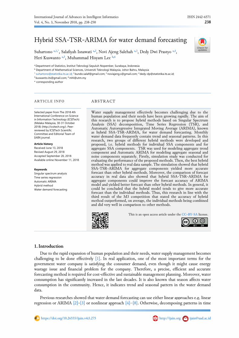
The SSA method decomposes the data (119885119905) into several subpart series (119875119862119905) The hybrid SSA-ARIMA model applies the idea of individual and aggregate component modeling In this research the framework of individual and aggregate SSA-ARIMA modeling are shown in Fig 1 and Fig 2 respectively [12]-[13]
Fig 1 Hybrid SSA-ARIMA of individual component for time series forecasting
The individual forecasting is done by modeling each series using the ARIMA method and calculate the fitted value for each eigentriple However specifically for eigentriple which has noise pattern the modeling is done in aggregate ie noise eigentriple is combined into noise component (119873119905) This component will be fitted using auto ARIMA so the forecast result of noise component (119905) is formed Finally the forecast was made by each SSA-component ftting have been summed up to make final forecast (119905)
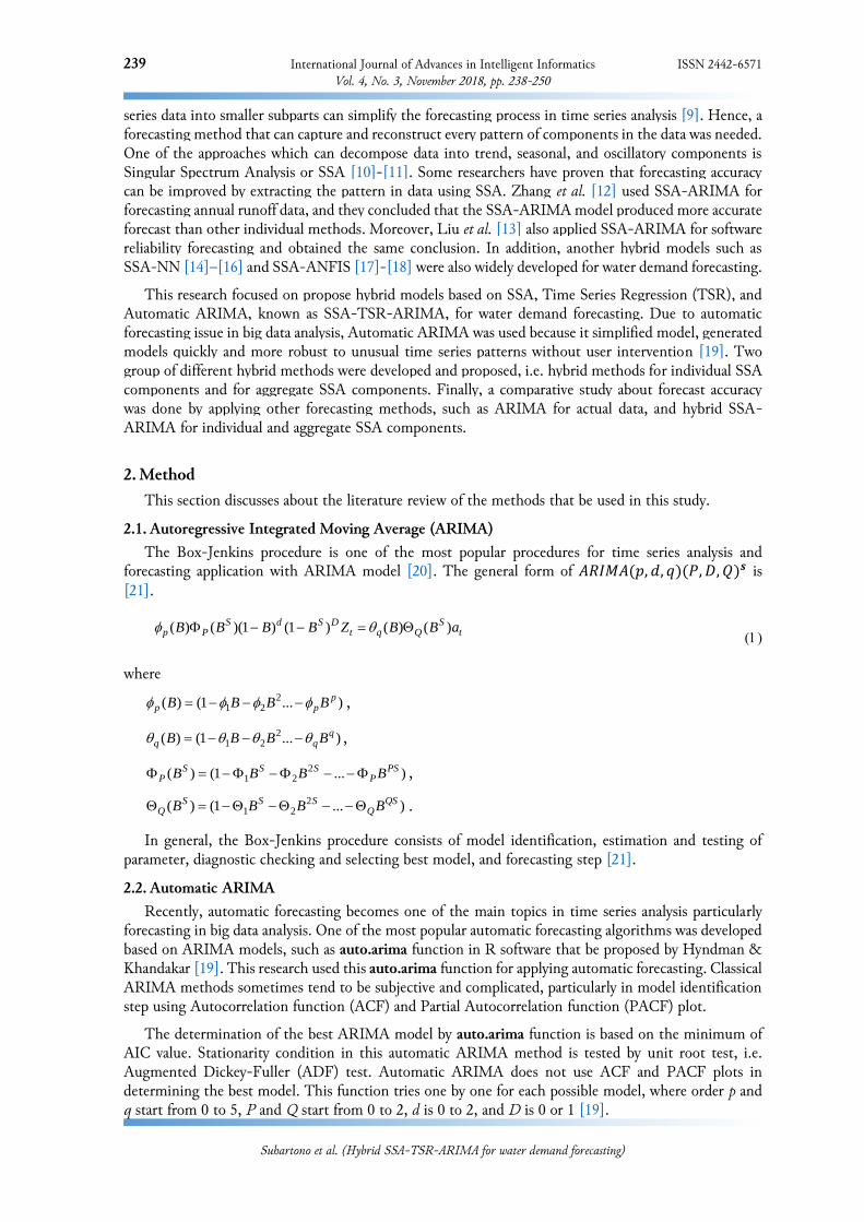
Fig 2 represents the framework of Aggregate SSA-ARIMA modeling In contrast to individual SSA-ARIMA modeling this model is performed by incorporating similar eigentriple Eigentriples that have
ISSN 2442-6571 International Journal of Advances in Intelligent Informatics 242 Vol 4 No 3 November 2018 pp 238-250
Suhartono et al (Hybrid SSA-TSR-ARIMA for water demand forecasting)
a similar pattern will be summed into one component Eigentriples that have a trend pattern summed into trend component (119879119905) and so do for seasonal (119878119905) and noise (119873119905) component Automatic ARIMA modeling is done on each SSA-component to produce the fitted values of trend (119905) seasonal (119905) and noise (119905) component The summation of each SSA-component fitting will lead to final forecast of the series (119905) Both in individual and aggregate modeling the trend seasonal and noise series will be approximated by Automatic ARIMA
Fig 2 Hybrid SSA-ARIMA of aggregate component for time series forecasting
26 The Proposed Hybrid SSA-TSR-ARIMA
The proposed hybrid method is mainly based on TSR for fitting trend component in aggregate modeling scenario The idea is motivated by the trend component of SSA-decomposition tend to follow polynomial trend pattern Thus TSR as equation (6) will capture well this pattern In general the proposed hybrid SSA-TSR-ARIMA method is illustrated as Fig 3
Fig 3 The proposed hybrid SSA-TSR-ARIMA for time series forecasting
27 Model Evaluation
The model evaluation is done based on both in-sample (training) and out-sample (testing) criteria Automatic ARIMA uses in-sample criteria for selecting the best model based on the smallest AIC or Akaikes Information Criterion as follows
2ˆln 2aAIC n C
where 2ˆa is maximum likelihood estimation of 2
a and C is number of parameters
243 International Journal of Advances in Intelligent Informatics ISSN 2442-6571
Vol 4 No 3 November 2018 pp 238-250
Suhartono et al (Hybrid SSA-TSR-ARIMA for water demand forecasting)
Furthermore the best model in this research was selected based on out-sample (testing) criteria as known as cross-validation principle Two criteria in testing data for determining the best model are Root Mean Square Error (RMSE) and Mean Absolute Percentage Error (MAPE) that be calculated as follows
2
1
1 ˆ( ( ))R
n r n
r
RMSE Y Y rR
1
ˆ ( )1100
Rn r n
n rr
Y Y rMAPE
R Y
where R is the forecast periods [25]
28 Real Data of Water Demand in Wonogiri Regency Indonesia
PDAM or Regional Company for Water Utility is one of the regional owned business units which is engaged in distributing and providing fresh water for the public PDAMs exist in every province district and municipality throughout Indonesia Wonogiri regency is one of the districts in Central Java province Indonesia The water needs are managed by PDAM in Wonogiri Regency based on the instruction of the Minister of Home Affairs Water demand could be detected by monitoring the amount of fresh water consumed by customers The calculation of water demand in Wonogiri is done every 20th date of the corresponding month Water demand data in February is calculated from 21 January to 20 February The water demand in March is calculated from February 21 to March 20 and so on Then the collected time series data will be used as a representative data on this work
3 Results and Discussion
This study conducted simulation and empirical study and this section discussed about the results and analysis of both studies
31 Simulation study
The purpose of the simulation study is to know the performance of the proposed hybrid method to forecast the time series with trend and seasonal pattern As discussed in the previous section the hybrid SSA-ARIMA method will be applied individually (written as first model or M-1) or aggregately (written as second model or M-2) and the proposed hybrid SSA-TSR-ARIMA method in aggregate scheme (written as third model or M-3) This study simulation was conducted by assuming for monthly data with periods from January 2006 to December 2017 or generated for 144 observations where 120 initial data as training dataset and last 24 data as testing dataset The simulation data that containing trend seasonal and noise components were generated as follows
t t t tY T S N
where 05 tT t for trend 2
75sin12
t
tS
for seasonal and ~ (01)tN N for noise components
The time series plot of the simulation data is shown in Fig 4
Each original series was decomposed by using SSA In this simulation data 50 eigentriple formed with 4 main eigentriples and 46 noise eigentriples The main eigentriple consists of two trend eigentriples and two seasonal eigentriples Similar patterned eigentriples were grouped in to the same component In general the trend component consists of two trend-patterned eigentriples a seasonal component consisting of two seasonal-patterned eigentriples and a noise component composed of 46 eigentriple noise patterns
ISSN 2442-6571 International Journal of Advances in Intelligent Informatics 244 Vol 4 No 3 November 2018 pp 238-250
Suhartono et al (Hybrid SSA-TSR-ARIMA for water demand forecasting)
201720162015201420132012201120102009200820072006
80
70
60
50
40
30
20
10
0
Time
Yt
Sim
ula
tion D
ata
Fig 4 Time Series Plot of Simulation Data that contain trend and seasonal
Then these decompositions series were modeled using hybrid SSA-ARIMA in individual and aggregate scheme and hybrid SSA-TSR-ARIMA in aggregate scheme The results were showed at Table 1
Table 1 Forecast Accuracy of Hybrid Methods in Simulation Data
Method ARIMA Model AIC Testing Dataset
MAPE RMSE
M-1 SSA-ARIMA (individually) 1269 1109
1PC
(121) -72222
2PC (124)(110)12 -55560
3PC (000)(110)12 18717
4PC (320) -56771
tN
(001) 30949
M-2 SSA-ARIMA (aggregate) 759 566
tT
(121) -72222
tS (010)(110)12 -8314
tN
(001) 30949
M-3 SSA-TSR-ARIMA (aggregate) 283 220
tT
ˆ tT -
tS (010)(110)12 -8314
tN
(001) 30949
2ˆ 0824 0467 0000266 tT t t
Table 1 showed that the proposed hybrid SSA-TSR-ARIMA in aggregate scheme outperformed other hybrid models ie yielded the lowest MAPE and RMSE Hence it indicated that in time series data containing trend and seasonal patterns the hybrid SSA-TSR-ARIMA under aggregate scheme produced the most accurate forecast at the testing dataset
32 Water Demand Forecasting
Consumer behavior in water demand can be seen from the characteristics of water consumption data This information can be used to make water resources planning to minimize the waste of water resources and company losses The monthly of water demand by community in Wonogiri regency Indonesia during the period January 2006 to August 2017 is shown in Fig 5
245 International Journal of Advances in Intelligent Informatics ISSN 2442-6571
Vol 4 No 3 November 2018 pp 238-250
Suhartono et al (Hybrid SSA-TSR-ARIMA for water demand forecasting)
201720162015201420132012201120102009200820072006
600000
550000
500000
450000
400000
350000
300000
Time
Wate
r Dem
and (
in m
3)
Fig 5 Time Series Plot of Monthly Water Demand in Wonogiri Regency Indonesia
The monthly water demand increased over time and has seasonal pattern (Fig 5) There are 140 observations with average monthly water demand of 4287 thousand m3 In this period the smallest demand occurred in March 2006 and the highest is in July 2017 ie 2994 and 5763 thousand m3 respectively Moreover due to dry season in Wonogiri regency the average water demand in August to November tends to be higher than other months
321 Hybrid SSA-ARIMA
SSA decomposition of the monthly water demand data generated 50 eigentriples (as shown in Fig 6a) which in the SVD stage produces 3 main eigentriples with 1 trend eigentriple and 2 seasonal eigentriples (as shown in Fig 6b) The noise component consists of 4 to 50 eigentriples Fig 6 and Fig 7 illustrate the reconstruction results of trend seasonal and noise components of monthly water demand data
(a)
(b)
Fig 6 Eigentriples (a) and Principal Component (b) plot of water demand
ISSN 2442-6571 International Journal of Advances in Intelligent Informatics 246 Vol 4 No 3 November 2018 pp 238-250
Suhartono et al (Hybrid SSA-TSR-ARIMA for water demand forecasting)
Due to the results of simulation study showed that hybrid SSA-ARIMA in aggregate scheme give better forecast than individual scheme then monthly water demand data were analyzed only by hybrid SSA-ARIMA in aggregate scheme Each component was modeled using Automatic ARIMA and the best model for trend seasonal and noise components were ARIMA(120) ARIMA(100)(111)12 and ARIMA(102)(100)12 respectively The MAPE and RMSE of this hybrid model in training dataset were 526 and 45900 respectively whereas at testing dataset were 1302 and 79039 respectively
(a)
10896847260483624121
550000
500000
450000
400000
350000
300000
Time
Trend
(b)
10896847260483624121
40000
30000
20000
10000
0
-10000
-20000
-30000
-40000
Time
Seasonal
A ug
Jul
Jun
May
A prMar
Feb
Jan
Dec
Nov
O ctSep
A ug
Jul
Jun
May
A prMar
Feb
Jan
Dec
Nov
O ctSep
A ug
Jul
Jun
May
A prMar
Feb
Jan
Dec
Nov
O ctSep
A ug
Jul
Jun
May
A prMar
Feb
Jan
Dec
Nov
O ctSep
A ug
Jul
Jun
May
A prMar
Feb
Jan
Dec
Nov
O ctSep
A ug
Jul
Jun
May
A prMar
Feb
Jan
Dec
Nov
O ctSep
A ug
Jul
Jun
May
A prMar
Feb
Jan
Dec
Nov
O ctSep
A ug
Jul
Jun
May
A prMar
Feb
Jan
Dec
Nov
O ctSep
A ug
Jul
Jun
May
A prMar
Feb
Jan
Dec
NovO ct
Sep
A ug
Jul
Jun
MayA pr
Mar
Feb
Jan
(c)
10896847260483624121
75000
50000
25000
0
-25000
-50000
Time
Noise
Fig 7 Grouping of Trend (a) Seasonal (b) and Noise (c) Components of Water Demand Data
247 International Journal of Advances in Intelligent Informatics ISSN 2442-6571
Vol 4 No 3 November 2018 pp 238-250
Suhartono et al (Hybrid SSA-TSR-ARIMA for water demand forecasting)
322 Hybrid SSA-TSR-ARIMA
The main difference between hybrid SSA-TSR-ARIMA and SSA-ARIMA in aggregate scheme is the modeling of trend component using polynomial regression instead of ARIMA model The model for trend component obtained from TSR is
2ˆ 318079 122587 4 4867tT t t
Moreover the MAPE and RMSE in training dataset of this hybrid SSA-TSR-ARIMA method were 382 and 20398 respectively whereas at testing dataset were 937 and 58751 respectively
323 The Results of ARIMA Model
The best ARIMA models for monthly water demand data was ARIMA(21[35])(110)12 This model has fulfilled white noise and normally distributed assumptions for the residual The equation of this ARIMA model is as follows
1 2 3 12 13 14 15
24 25 26 27 35
034 036 029 071 012 025 020
029 010 010 008 050
t t t t t t t t
t t t t t t
Z Z Z Z Z Z Z Z
Z Z Z Z a a
where 1t tZ Z The MAPE and RMSE in training dataset of this ARIMA model were 424 and
22940 respectively whereas at testing dataset were 964 and 60836 respectively
324 Model Selection and Forecast Accuracy Comparison
Three forecasting methods have been applied for forecasting monthly water demand data in Wonogiri regency ie ARIMA hybrid SSA-ARIMA and hybrid SSA-TSR-ARIMA methods The actual and forecasted values of water demand at testing dataset are shown in Fig 8
Fig 8 The Actual and Forecast Values of Water Demand at Testing Dataset
Moreover a numerical evaluation based on RMSE and MAPE for both training and testing datasets to provide more precise comparison on the performance of this water demand forecasting from each model was done and presented in Table 2 Column ratio of MAPE and RMSE showed the ratio values to ARIMA model
In general the results at Table 2 provided two contradictive conclusions about the hybrid or combination methods (or complex method) compared to individual or simple methods The first comparison between ARIMA and hybrid SSA-ARIMA showed that ARIMA as a simple method yielded more accurate forecast than hybrid SSA-ARIMA as a complex method Moreover this first result was in line with the first result of M3 competition that stated statistically sophisticated or complex methods do not necessarily provide more accurate forecasts than simpler ones [26] Otherwise this first result did not in line with the results from Zhang et al [12] and Liu et al [13]
ISSN 2442-6571 International Journal of Advances in Intelligent Informatics 248 Vol 4 No 3 November 2018 pp 238-250
Suhartono et al (Hybrid SSA-TSR-ARIMA for water demand forecasting)
Table 2 Comparison Results of Accuracy Performance for each Model
Model Training Dataset Testing Dataset Ratio
MAPE RMSE MAPE RMSE MAPE RMSE
SSA-ARIMA 526 45900 1302 79039 135 132
SSA-TSR-ARIMA 382 20398 937 58751 097 097
ARIMA 424 22940 964 60836 100 100
Furthermore the second comparison between hybrid SSA-TSR-ARIMA hybrid SSA-ARIMA and ARIMA showed that hybrid SSA-TSR-ARIMA method as combination method provided better forecast than hybrid SSA-ARIMA as a simpler method and ARIMA as an individual method Thus this second result was in line with the third result of M3 competition that stated the accuracy when various methods were being combined outperforms on average the individual methods being combined and did very well in comparison to other methods [26]ndash[28] In addition this second result also showed that forecaster must understand well the advantage of each model before combining particularly the relation between model and the time series pattern that could be handled it
In general the results on Table 2 showed that the best method for water demand forecasting in Wonogiri regency was the proposed hybrid SSA-TSR-ARIMA in aggregate scheme Moreover this proposed method provided more accurate forecast both in training and testing dataset by using MAPE and RMSE criteria The greater values of MAPE and RMSE in testing dataset compared to in training dataset was caused by the fluctuation of trend behavior change lower in testing dataset If there is such a change due to a special event the resulting forecast of SSA decomposition tends to be grouped into other components and can produce misleading forecasts [29]
4 Conclusion
This research proposed a hybrid SSA-TSR-ARIMA method for water demand forecasting The results of simulation study showed that hybrid SSA-ARIMA method in aggregate scheme yielded more accurate forecast than individual scheme Moreover the simulation study also showed that the proposed hybrid SSA-TSR-ARIMA method in aggregate scheme provided better forecast than hybrid SSA-ARIMA method both in aggregate and individual scheme Additionally the results of simulation study also showed that SSA decomposition was appropriately applied on time series data containing trend seasonal and noise components [30]
Furthermore the results of real data about monthly water demand forecasting in Wonogiri regency showed that the proposed hybrid SSA-TSR-ARIMA in aggregate scheme as a combining some individual methods provided more accurate forecast than hybrid SSA-ARIMA as a simpler method and ARIMA as an individual method Thus these results in line with the third result of M3 forecasting competition that be done by Makridakis amp Hibon [26] Moreover this study also clearly shown that by applying TSR for fitting the trend component of SSA decomposition can increase the accuracy of the prediction compared to only applying ARIMA directly to actual data or to each SSA component This leads a suggestion for further research particularly by involving nonlinear methods (such as neural networks deep learning networks or ANFIS) when combining to SSA for handling nonlinearity issue in time series forecasting
Acknowledgment
This study was supported by DRPM-DIKTI under scheme of ldquoPenelitian Berbasis Kompetensirdquo project No 851PKSITS2018 The authors thank to the General Director of DIKTI for funding and to anonymous referees for their useful suggestions
References
[1] W J Cosgrove and D P Loucks ldquoWater management Current and future challenges and research directionsrdquo Water Resour Res vol 51 no 6 pp 4823ndash4839 Jun 2015 doi httpsdoiorg1010022014WR016869
249 International Journal of Advances in Intelligent Informatics ISSN 2442-6571
Vol 4 No 3 November 2018 pp 238-250
Suhartono et al (Hybrid SSA-TSR-ARIMA for water demand forecasting)
[2] J Adamowski H Fung Chan S O Prasher B Ozga-Zielinski and A Sliusarieva ldquoComparison of multiple linear and nonlinear regression autoregressive integrated moving average artificial neural network and wavelet artificial neural network methods for urban water demand forecasting in Montreal Canadardquo Water Resour Res vol 48 no 1 Jan 2012 doi httpsdoiorg1010292010WR009945
[3] A S Polebitski and R N Palmer ldquoSeasonal residential water demand forecasting for census tractsrdquo J Water Resour Plan Manag vol 136 no 1 pp 27ndash36 2009 doi httpsdoiorg101061(ASCE)WR1943-54520000003
[4] S P Zhang H Watanabe and R Yamada ldquoPrediction of Daily Water Demands by Neural Networksrdquo 1994 pp 217ndash227 doi httpsdoiorg101007978-94-017-3083-9_17
[5] J Bougadis K Adamowski and R Diduch ldquoShort-term municipal water demand forecastingrdquo Hydrol Process An Int J vol 19 no 1 pp 137ndash148 2005 doi httpsdoiorg101002hyp5763
[6] J F Adamowski ldquoPeak daily water demand forecast modeling using artificial neural networksrdquo J Water Resour Plan Manag vol 134 no 2 pp 119ndash128 2008 doi httpsdoiorg101061(ASCE)0733-9496(2008)1342(119)
[7] M Ghiassi D K Zimbra and H Saidane ldquoUrban water demand forecasting with a dynamic artificial neural network modelrdquo J Water Resour Plan Manag vol 134 no 2 pp 138ndash146 2008 doi httpsdoiorg101061(ASCE)0733-9496(2008)1342(138)
[8] M Herrera L Torgo J Izquierdo and R Peacuterez-Garciacutea ldquoPredictive models for forecasting hourly urban water demandrdquo J Hydrol vol 387 no 1ndash2 pp 141ndash150 Jun 2010 doi httpsdoiorg101016jjhydrol201004005
[9] B L Bowerman and R T OrsquoConnell ldquoForecasting and time series An applied approach 3rdrdquo 1993 available at httpecsocmanhserutext19151946
[10] N Golyandina V Nekrutkin and A Zhigljavsky Analysis of Time Series Structure 2001 vol 90 doi httpsdoiorg1012019781420035841
[11] J Liao L Gao and X Wang ldquoNumerical Simulation and Forecasting of Water Level for Qinghai Lake Using Multi-Altimeter Data Between 2002 and 2012rdquo IEEE J Sel Top Appl Earth Obs Remote Sens vol 7 no 2 pp 609ndash622 Feb 2014 doi httpsdoiorg101109JSTARS20132291516
[12] Q Zhang B-D Wang B He Y Peng and M-L Ren ldquoSingular Spectrum Analysis and ARIMA Hybrid Model for Annual Runoff Forecastingrdquo Water Resour Manag vol 25 no 11 pp 2683ndash2703 Sep 2011 doi httpsdoiorg101007s11269-011-9833-y
[13] G Liu D Zhang and T Zhang ldquoSoftware Reliability Forecasting Singular Spectrum Analysis and ARIMA Hybrid Modelrdquo in 2015 International Symposium on Theoretical Aspects of Software Engineering 2015 pp 111ndash118 doi httpsdoiorg101109TASE201519
[14] S L Zubaidi J Dooley R M Alkhaddar M Abdellatif H Al-Bugharbee and S Ortega-Martorell ldquoA Novel approach for predicting monthly water demand by combining singular spectrum analysis with neural networksrdquo J Hydrol vol 561 pp 136ndash145 Jun 2018 doi httpsdoiorg101016jjhydrol201803047
[15] M Sun X Li and G Kim ldquoPrecipitation analysis and forecasting using singular spectrum analysis with artificial neural networksrdquo Cluster Comput Jan 2018 doi httpsdoiorg101007s10586-018-1713-2
[16] L Latifoğlu Ouml Kişi and F Latifoğlu ldquoImportance of hybrid models for forecasting of hydrological variablerdquo Neural Comput Appl vol 26 no 7 pp 1669ndash1680 Oct 2015 doi httpsdoiorg101007s00521-015-1831-1
[17] Y Xiao J J Liu Y Hu Y Wang K K Lai and S Wang ldquoA neuro-fuzzy combination model based on singular spectrum analysis for air transport demand forecastingrdquo J Air Transp Manag vol 39 pp 1ndash11 Jul 2014 doi httpsdoiorg101016jjairtraman201403004
[18] M Abdollahzade A Miranian H Hassani and H Iranmanesh ldquoA new hybrid enhanced local linear neuro-fuzzy model based on the optimized singular spectrum analysis and its application for nonlinear and chaotic time series forecastingrdquo Inf Sci (Ny) vol 295 pp 107ndash125 Feb 2015 doi httpsdoiorg101016jins201409002
ISSN 2442-6571 International Journal of Advances in Intelligent Informatics 250 Vol 4 No 3 November 2018 pp 238-250
Suhartono et al (Hybrid SSA-TSR-ARIMA for water demand forecasting)
[19] R J Hyndman and Y Khandakar Automatic time series for forecasting the forecast package for R no 607 Monash University Department of Econometrics and Business Statistics 2007 available at httpwebdocsubgwdgdeebookserienemonash_univwp6-07pdf
[20] G E P Box G M Jenkins and G C Reinsel Time Series Analysis Forecasting and Control 3rd ed Prentice Hall 1994 available at httpsbooksgooglecombooksid=sRzvAAAAMAAJ
[21] W W S Wei Time Series Analysis Univariate and Multivariate Methods Pearson Addison Wesley 2006 available at httpsbooksgooglecombooksid=aY0QAQAAIAAJ
[22] N Golyandina and A Zhigljavsky Singular Spectrum Analysis for Time Series 2013 doi httpsdoiorg101007978-3-642-34913-3
[23] H Hassani ldquoSingular spectrum analysis methodology and comparisonrdquo J Data Sci vol 5 no 2 pp 239ndash257 2007 available at httpsmpraubuni-muenchende4991
[24] R J Hyndman and G Athanasopoulos Forecasting principles and practice OTexts 2018 available at httpsbooksgooglecombooksid=_bBhDwAAQBAJ
[25] R J Hyndman and A B Koehler ldquoAnother look at measures of forecast accuracyrdquo Int J Forecast vol 22 no 4 pp 679ndash688 Oct 2006 doi httpsdoiorg101016jijforecast200603001
[26] S Makridakis and M Hibon ldquoThe M3-Competition results conclusions and implicationsrdquo Int J Forecast vol 16 no 4 pp 451ndash476 Oct 2000 doi httpsdoiorg101016S0169-2070(00)00057-1
[27] Suhartono and M H Lee ldquoA Hybrid Approach based on Winterrsquos Model and Weighted Fuzzy Time Series for Forecasting Trend and Seasonal Datardquo J Math Stat vol 7 no 3 pp 177ndash183 2011 doi httpsdoiorg103844jmssp2011177183
[28] Suhartono I Puspitasari M S Akbar M H Lee ldquoTwo-level seasonal model based on hybrid ARIMA-ANFIS for forecasting short-term electricity load in Indonesiardquo in Statistics in Science Business and Engineering (ICSSBE) 2012 International Conference on 2012 pp 1ndash5 doi httpsdoiorg101109ICSSBE20126396642
[29] H Hassani A S Soofi and A A Zhigljavsky ldquoPredicting daily exchange rate with singular spectrum analysisrdquo Nonlinear Anal Real World Appl vol 11 no 3 pp 2023ndash2034 Jun 2010 doi httpsdoiorg101016jnonrwa200905008
[30] W Sulandari Suhartono Subanar and H Utami ldquoForecasting time series with trend and seasonal patterns based on SSArdquo in Science in Information Technology (ICSITech) 2017 3rd International Conference on 2017 pp 648ndash653 doi httpsdoiorg101109ICSITech20178257193
239 International Journal of Advances in Intelligent Informatics ISSN 2442-6571
Vol 4 No 3 November 2018 pp 238-250
Suhartono et al (Hybrid SSA-TSR-ARIMA for water demand forecasting)
series data into smaller subparts can simplify the forecasting process in time series analysis [9] Hence a forecasting method that can capture and reconstruct every pattern of components in the data was needed One of the approaches which can decompose data into trend seasonal and oscillatory components is Singular Spectrum Analysis or SSA [10]-[11] Some researchers have proven that forecasting accuracy can be improved by extracting the pattern in data using SSA Zhang et al [12] used SSA-ARIMA for forecasting annual runoff data and they concluded that the SSA-ARIMA model produced more accurate forecast than other individual methods Moreover Liu et al [13] also applied SSA-ARIMA for software reliability forecasting and obtained the same conclusion In addition another hybrid models such as SSA-NN [14]ndash[16] and SSA-ANFIS [17]-[18] were also widely developed for water demand forecasting
This research focused on propose hybrid models based on SSA Time Series Regression (TSR) and Automatic ARIMA known as SSA-TSR-ARIMA for water demand forecasting Due to automatic forecasting issue in big data analysis Automatic ARIMA was used because it simplified model generated models quickly and more robust to unusual time series patterns without user intervention [19] Two group of different hybrid methods were developed and proposed ie hybrid methods for individual SSA components and for aggregate SSA components Finally a comparative study about forecast accuracy was done by applying other forecasting methods such as ARIMA for actual data and hybrid SSA-ARIMA for individual and aggregate SSA components
2 Method
This section discusses about the literature review of the methods that be used in this study
21 Autoregressive Integrated Moving Average (ARIMA)
The Box-Jenkins procedure is one of the most popular procedures for time series analysis and forecasting application with ARIMA model [20] The general form of 119860119877119868119872119860(119901 119889 119902)(119875 119863 119876)119956 is [21]
( ) ( )(1 ) (1 ) ( ) ( )S d S D Sp P t q Q tB B B B Z B B a
where
21 2( ) (1 )p
p pB B B B
21 2( ) (1 )q
q qB B B B
21 2( ) (1 )S S S PS
P PB B B B
21 2( ) (1 )S S S QS
Q QB B B B
In general the Box-Jenkins procedure consists of model identification estimation and testing of parameter diagnostic checking and selecting best model and forecasting step [21]
22 Automatic ARIMA
Recently automatic forecasting becomes one of the main topics in time series analysis particularly forecasting in big data analysis One of the most popular automatic forecasting algorithms was developed based on ARIMA models such as autoarima function in R software that be proposed by Hyndman amp Khandakar [19] This research used this autoarima function for applying automatic forecasting Classical ARIMA methods sometimes tend to be subjective and complicated particularly in model identification step using Autocorrelation function (ACF) and Partial Autocorrelation function (PACF) plot
The determination of the best ARIMA model by autoarima function is based on the minimum of AIC value Stationarity condition in this automatic ARIMA method is tested by unit root test ie Augmented Dickey-Fuller (ADF) test Automatic ARIMA does not use ACF and PACF plots in determining the best model This function tries one by one for each possible model where order p and q start from 0 to 5 P and Q start from 0 to 2 d is 0 to 2 and D is 0 or 1 [19]
ISSN 2442-6571 International Journal of Advances in Intelligent Informatics 240 Vol 4 No 3 November 2018 pp 238-250
Suhartono et al (Hybrid SSA-TSR-ARIMA for water demand forecasting)
23 Singular Spectrum Analysis
Singular Spectrum Analysis (SSA) is known as a powerful method for time series analysis SSA combines elements of classical time series analysis multivariate statistics multivariate geometric dynamical system and signal processing [22] The main purpose of SSA is to decipher the original series into a small number of identifiable components such as trend seasonal and oscillatory followed by the reconstruction of the original series [23] There are two main stages in SSA as follows
231 Decomposition (embedding and singular value decomposition)
Given a real-valued time series 1 2( )nY Y Y and L is an integer number denoted for window length
1 L n In embedding step the original time series will be mapped into a trajectory matrix which
illustrated as follows
1 2 3
2 3 4 1
1 3 4 5 2
1 2
[ ]
K
K
K K
L L L n
f f f f
f f f f
X X f f f f
f f f f
X
where 1K n L and T1 1( ) 1i i i i LX f f f i K Let 1 2 L be the eigenvalues of
the covariance matrix TS XX and 1 2 LU U U are the corresponding eigenvectors That eigenvalues
are arranged in a decreasing order 1 2 0L In second step the SVD of matrix X can be
stated as follows
1 2 d X X X X
where Ti i i iU VX The set ( )i i iU V is called i-th eigentriple to SVD
232 Reconstruction (grouping and diagonal averaging)
In grouping step the set of indices 1 2 d will be partitioned into m disjoint subsets 1 2 mI I I
and let 1 2 pI i i i Then the resultant matrix IX corresponds to group I defined as
1 1
pI i i i X X X X Computing these matrixes for groups 1 2 mI I I I and lead to
decomposition form 1 2
mI I I X X X X The set 1 2 mI I I are called eigentriple groupings
In the last step each elementary matrix in the grouped decomposition is transformed into a new component series Let i jy be the element of matrix Y (119871 times 119870 matrix) 1 le 119894 le 119871 1 le 119895 le 119870 for
119871 le 119870 Given the values of min( )L L K max( )K L K and 1n L K Let ii j jy y If
L K and let i j j iy y if L K otherwise Diagonal averaging transforms matrix Y into the series
1 2 ng g g by the formula
1
1
1
1
1
1
1
1 for 1
1 for
1 for
1
k
m k m
m
L
k m k m
m
n K
m k m
m k K
y k Lk
g y L k KL
y K k nn k
241 International Journal of Advances in Intelligent Informatics ISSN 2442-6571
Vol 4 No 3 November 2018 pp 238-250
Suhartono et al (Hybrid SSA-TSR-ARIMA for water demand forecasting)
The equation corresponds to the average matrix element over the lsquoantidiagonalsrsquo 1i j k If the
averaging diagonal is applied to the matrix IkX then a reconstructed series ( ) ( )( ) ( )1 2( )
k kk knF f f f
with length n will be obtained Therefore the initial series can be reconstructed by summation as follows
( )
1
12 m
kj j
k
f f j n
24 Time Series Regression
Basically TSR is the same as regression particularly with regression with dummy variables In this research the TSR model is a model for handling trend and seasonal components separately In general the trend is defined as the long-term direction that is continuously up or down and seasonality is a repeating pattern with the same period for example 12 months per year [24]
The TSR model for trend pattern can be described as polynomial regression as follows
20 1 2
ˆ mt mT t t t
whereas the TSR model for seasonal pattern in general is written as follows
1 1 2 2ˆ t s sS D D D
where 119863119895 (for 119895 = 12hellip 119904) are dummy variables for seasonal component
25 Hybrid SSA-ARIMA
The SSA method decomposes the data (119885119905) into several subpart series (119875119862119905) The hybrid SSA-ARIMA model applies the idea of individual and aggregate component modeling In this research the framework of individual and aggregate SSA-ARIMA modeling are shown in Fig 1 and Fig 2 respectively [12]-[13]
Fig 1 Hybrid SSA-ARIMA of individual component for time series forecasting
The individual forecasting is done by modeling each series using the ARIMA method and calculate the fitted value for each eigentriple However specifically for eigentriple which has noise pattern the modeling is done in aggregate ie noise eigentriple is combined into noise component (119873119905) This component will be fitted using auto ARIMA so the forecast result of noise component (119905) is formed Finally the forecast was made by each SSA-component ftting have been summed up to make final forecast (119905)
Fig 2 represents the framework of Aggregate SSA-ARIMA modeling In contrast to individual SSA-ARIMA modeling this model is performed by incorporating similar eigentriple Eigentriples that have
ISSN 2442-6571 International Journal of Advances in Intelligent Informatics 242 Vol 4 No 3 November 2018 pp 238-250
Suhartono et al (Hybrid SSA-TSR-ARIMA for water demand forecasting)
a similar pattern will be summed into one component Eigentriples that have a trend pattern summed into trend component (119879119905) and so do for seasonal (119878119905) and noise (119873119905) component Automatic ARIMA modeling is done on each SSA-component to produce the fitted values of trend (119905) seasonal (119905) and noise (119905) component The summation of each SSA-component fitting will lead to final forecast of the series (119905) Both in individual and aggregate modeling the trend seasonal and noise series will be approximated by Automatic ARIMA
Fig 2 Hybrid SSA-ARIMA of aggregate component for time series forecasting
26 The Proposed Hybrid SSA-TSR-ARIMA
The proposed hybrid method is mainly based on TSR for fitting trend component in aggregate modeling scenario The idea is motivated by the trend component of SSA-decomposition tend to follow polynomial trend pattern Thus TSR as equation (6) will capture well this pattern In general the proposed hybrid SSA-TSR-ARIMA method is illustrated as Fig 3
Fig 3 The proposed hybrid SSA-TSR-ARIMA for time series forecasting
27 Model Evaluation
The model evaluation is done based on both in-sample (training) and out-sample (testing) criteria Automatic ARIMA uses in-sample criteria for selecting the best model based on the smallest AIC or Akaikes Information Criterion as follows
2ˆln 2aAIC n C
where 2ˆa is maximum likelihood estimation of 2
a and C is number of parameters
243 International Journal of Advances in Intelligent Informatics ISSN 2442-6571
Vol 4 No 3 November 2018 pp 238-250
Suhartono et al (Hybrid SSA-TSR-ARIMA for water demand forecasting)
Furthermore the best model in this research was selected based on out-sample (testing) criteria as known as cross-validation principle Two criteria in testing data for determining the best model are Root Mean Square Error (RMSE) and Mean Absolute Percentage Error (MAPE) that be calculated as follows
2
1
1 ˆ( ( ))R
n r n
r
RMSE Y Y rR
1
ˆ ( )1100
Rn r n
n rr
Y Y rMAPE
R Y
where R is the forecast periods [25]
28 Real Data of Water Demand in Wonogiri Regency Indonesia
PDAM or Regional Company for Water Utility is one of the regional owned business units which is engaged in distributing and providing fresh water for the public PDAMs exist in every province district and municipality throughout Indonesia Wonogiri regency is one of the districts in Central Java province Indonesia The water needs are managed by PDAM in Wonogiri Regency based on the instruction of the Minister of Home Affairs Water demand could be detected by monitoring the amount of fresh water consumed by customers The calculation of water demand in Wonogiri is done every 20th date of the corresponding month Water demand data in February is calculated from 21 January to 20 February The water demand in March is calculated from February 21 to March 20 and so on Then the collected time series data will be used as a representative data on this work
3 Results and Discussion
This study conducted simulation and empirical study and this section discussed about the results and analysis of both studies
31 Simulation study
The purpose of the simulation study is to know the performance of the proposed hybrid method to forecast the time series with trend and seasonal pattern As discussed in the previous section the hybrid SSA-ARIMA method will be applied individually (written as first model or M-1) or aggregately (written as second model or M-2) and the proposed hybrid SSA-TSR-ARIMA method in aggregate scheme (written as third model or M-3) This study simulation was conducted by assuming for monthly data with periods from January 2006 to December 2017 or generated for 144 observations where 120 initial data as training dataset and last 24 data as testing dataset The simulation data that containing trend seasonal and noise components were generated as follows
t t t tY T S N
where 05 tT t for trend 2
75sin12
t
tS
for seasonal and ~ (01)tN N for noise components
The time series plot of the simulation data is shown in Fig 4
Each original series was decomposed by using SSA In this simulation data 50 eigentriple formed with 4 main eigentriples and 46 noise eigentriples The main eigentriple consists of two trend eigentriples and two seasonal eigentriples Similar patterned eigentriples were grouped in to the same component In general the trend component consists of two trend-patterned eigentriples a seasonal component consisting of two seasonal-patterned eigentriples and a noise component composed of 46 eigentriple noise patterns
ISSN 2442-6571 International Journal of Advances in Intelligent Informatics 244 Vol 4 No 3 November 2018 pp 238-250
Suhartono et al (Hybrid SSA-TSR-ARIMA for water demand forecasting)
201720162015201420132012201120102009200820072006
80
70
60
50
40
30
20
10
0
Time
Yt
Sim
ula
tion D
ata
Fig 4 Time Series Plot of Simulation Data that contain trend and seasonal
Then these decompositions series were modeled using hybrid SSA-ARIMA in individual and aggregate scheme and hybrid SSA-TSR-ARIMA in aggregate scheme The results were showed at Table 1
Table 1 Forecast Accuracy of Hybrid Methods in Simulation Data
Method ARIMA Model AIC Testing Dataset
MAPE RMSE
M-1 SSA-ARIMA (individually) 1269 1109
1PC
(121) -72222
2PC (124)(110)12 -55560
3PC (000)(110)12 18717
4PC (320) -56771
tN
(001) 30949
M-2 SSA-ARIMA (aggregate) 759 566
tT
(121) -72222
tS (010)(110)12 -8314
tN
(001) 30949
M-3 SSA-TSR-ARIMA (aggregate) 283 220
tT
ˆ tT -
tS (010)(110)12 -8314
tN
(001) 30949
2ˆ 0824 0467 0000266 tT t t
Table 1 showed that the proposed hybrid SSA-TSR-ARIMA in aggregate scheme outperformed other hybrid models ie yielded the lowest MAPE and RMSE Hence it indicated that in time series data containing trend and seasonal patterns the hybrid SSA-TSR-ARIMA under aggregate scheme produced the most accurate forecast at the testing dataset
32 Water Demand Forecasting
Consumer behavior in water demand can be seen from the characteristics of water consumption data This information can be used to make water resources planning to minimize the waste of water resources and company losses The monthly of water demand by community in Wonogiri regency Indonesia during the period January 2006 to August 2017 is shown in Fig 5
245 International Journal of Advances in Intelligent Informatics ISSN 2442-6571
Vol 4 No 3 November 2018 pp 238-250
Suhartono et al (Hybrid SSA-TSR-ARIMA for water demand forecasting)
201720162015201420132012201120102009200820072006
600000
550000
500000
450000
400000
350000
300000
Time
Wate
r Dem
and (
in m
3)
Fig 5 Time Series Plot of Monthly Water Demand in Wonogiri Regency Indonesia
The monthly water demand increased over time and has seasonal pattern (Fig 5) There are 140 observations with average monthly water demand of 4287 thousand m3 In this period the smallest demand occurred in March 2006 and the highest is in July 2017 ie 2994 and 5763 thousand m3 respectively Moreover due to dry season in Wonogiri regency the average water demand in August to November tends to be higher than other months
321 Hybrid SSA-ARIMA
SSA decomposition of the monthly water demand data generated 50 eigentriples (as shown in Fig 6a) which in the SVD stage produces 3 main eigentriples with 1 trend eigentriple and 2 seasonal eigentriples (as shown in Fig 6b) The noise component consists of 4 to 50 eigentriples Fig 6 and Fig 7 illustrate the reconstruction results of trend seasonal and noise components of monthly water demand data
(a)
(b)
Fig 6 Eigentriples (a) and Principal Component (b) plot of water demand
ISSN 2442-6571 International Journal of Advances in Intelligent Informatics 246 Vol 4 No 3 November 2018 pp 238-250
Suhartono et al (Hybrid SSA-TSR-ARIMA for water demand forecasting)
Due to the results of simulation study showed that hybrid SSA-ARIMA in aggregate scheme give better forecast than individual scheme then monthly water demand data were analyzed only by hybrid SSA-ARIMA in aggregate scheme Each component was modeled using Automatic ARIMA and the best model for trend seasonal and noise components were ARIMA(120) ARIMA(100)(111)12 and ARIMA(102)(100)12 respectively The MAPE and RMSE of this hybrid model in training dataset were 526 and 45900 respectively whereas at testing dataset were 1302 and 79039 respectively
(a)
10896847260483624121
550000
500000
450000
400000
350000
300000
Time
Trend
(b)
10896847260483624121
40000
30000
20000
10000
0
-10000
-20000
-30000
-40000
Time
Seasonal
A ug
Jul
Jun
May
A prMar
Feb
Jan
Dec
Nov
O ctSep
A ug
Jul
Jun
May
A prMar
Feb
Jan
Dec
Nov
O ctSep
A ug
Jul
Jun
May
A prMar
Feb
Jan
Dec
Nov
O ctSep
A ug
Jul
Jun
May
A prMar
Feb
Jan
Dec
Nov
O ctSep
A ug
Jul
Jun
May
A prMar
Feb
Jan
Dec
Nov
O ctSep
A ug
Jul
Jun
May
A prMar
Feb
Jan
Dec
Nov
O ctSep
A ug
Jul
Jun
May
A prMar
Feb
Jan
Dec
Nov
O ctSep
A ug
Jul
Jun
May
A prMar
Feb
Jan
Dec
Nov
O ctSep
A ug
Jul
Jun
May
A prMar
Feb
Jan
Dec
NovO ct
Sep
A ug
Jul
Jun
MayA pr
Mar
Feb
Jan
(c)
10896847260483624121
75000
50000
25000
0
-25000
-50000
Time
Noise
Fig 7 Grouping of Trend (a) Seasonal (b) and Noise (c) Components of Water Demand Data
247 International Journal of Advances in Intelligent Informatics ISSN 2442-6571
Vol 4 No 3 November 2018 pp 238-250
Suhartono et al (Hybrid SSA-TSR-ARIMA for water demand forecasting)
322 Hybrid SSA-TSR-ARIMA
The main difference between hybrid SSA-TSR-ARIMA and SSA-ARIMA in aggregate scheme is the modeling of trend component using polynomial regression instead of ARIMA model The model for trend component obtained from TSR is
2ˆ 318079 122587 4 4867tT t t
Moreover the MAPE and RMSE in training dataset of this hybrid SSA-TSR-ARIMA method were 382 and 20398 respectively whereas at testing dataset were 937 and 58751 respectively
323 The Results of ARIMA Model
The best ARIMA models for monthly water demand data was ARIMA(21[35])(110)12 This model has fulfilled white noise and normally distributed assumptions for the residual The equation of this ARIMA model is as follows
1 2 3 12 13 14 15
24 25 26 27 35
034 036 029 071 012 025 020
029 010 010 008 050
t t t t t t t t
t t t t t t
Z Z Z Z Z Z Z Z
Z Z Z Z a a
where 1t tZ Z The MAPE and RMSE in training dataset of this ARIMA model were 424 and
22940 respectively whereas at testing dataset were 964 and 60836 respectively
324 Model Selection and Forecast Accuracy Comparison
Three forecasting methods have been applied for forecasting monthly water demand data in Wonogiri regency ie ARIMA hybrid SSA-ARIMA and hybrid SSA-TSR-ARIMA methods The actual and forecasted values of water demand at testing dataset are shown in Fig 8
Fig 8 The Actual and Forecast Values of Water Demand at Testing Dataset
Moreover a numerical evaluation based on RMSE and MAPE for both training and testing datasets to provide more precise comparison on the performance of this water demand forecasting from each model was done and presented in Table 2 Column ratio of MAPE and RMSE showed the ratio values to ARIMA model
In general the results at Table 2 provided two contradictive conclusions about the hybrid or combination methods (or complex method) compared to individual or simple methods The first comparison between ARIMA and hybrid SSA-ARIMA showed that ARIMA as a simple method yielded more accurate forecast than hybrid SSA-ARIMA as a complex method Moreover this first result was in line with the first result of M3 competition that stated statistically sophisticated or complex methods do not necessarily provide more accurate forecasts than simpler ones [26] Otherwise this first result did not in line with the results from Zhang et al [12] and Liu et al [13]
ISSN 2442-6571 International Journal of Advances in Intelligent Informatics 248 Vol 4 No 3 November 2018 pp 238-250
Suhartono et al (Hybrid SSA-TSR-ARIMA for water demand forecasting)
Table 2 Comparison Results of Accuracy Performance for each Model
Model Training Dataset Testing Dataset Ratio
MAPE RMSE MAPE RMSE MAPE RMSE
SSA-ARIMA 526 45900 1302 79039 135 132
SSA-TSR-ARIMA 382 20398 937 58751 097 097
ARIMA 424 22940 964 60836 100 100
Furthermore the second comparison between hybrid SSA-TSR-ARIMA hybrid SSA-ARIMA and ARIMA showed that hybrid SSA-TSR-ARIMA method as combination method provided better forecast than hybrid SSA-ARIMA as a simpler method and ARIMA as an individual method Thus this second result was in line with the third result of M3 competition that stated the accuracy when various methods were being combined outperforms on average the individual methods being combined and did very well in comparison to other methods [26]ndash[28] In addition this second result also showed that forecaster must understand well the advantage of each model before combining particularly the relation between model and the time series pattern that could be handled it
In general the results on Table 2 showed that the best method for water demand forecasting in Wonogiri regency was the proposed hybrid SSA-TSR-ARIMA in aggregate scheme Moreover this proposed method provided more accurate forecast both in training and testing dataset by using MAPE and RMSE criteria The greater values of MAPE and RMSE in testing dataset compared to in training dataset was caused by the fluctuation of trend behavior change lower in testing dataset If there is such a change due to a special event the resulting forecast of SSA decomposition tends to be grouped into other components and can produce misleading forecasts [29]
4 Conclusion
This research proposed a hybrid SSA-TSR-ARIMA method for water demand forecasting The results of simulation study showed that hybrid SSA-ARIMA method in aggregate scheme yielded more accurate forecast than individual scheme Moreover the simulation study also showed that the proposed hybrid SSA-TSR-ARIMA method in aggregate scheme provided better forecast than hybrid SSA-ARIMA method both in aggregate and individual scheme Additionally the results of simulation study also showed that SSA decomposition was appropriately applied on time series data containing trend seasonal and noise components [30]
Furthermore the results of real data about monthly water demand forecasting in Wonogiri regency showed that the proposed hybrid SSA-TSR-ARIMA in aggregate scheme as a combining some individual methods provided more accurate forecast than hybrid SSA-ARIMA as a simpler method and ARIMA as an individual method Thus these results in line with the third result of M3 forecasting competition that be done by Makridakis amp Hibon [26] Moreover this study also clearly shown that by applying TSR for fitting the trend component of SSA decomposition can increase the accuracy of the prediction compared to only applying ARIMA directly to actual data or to each SSA component This leads a suggestion for further research particularly by involving nonlinear methods (such as neural networks deep learning networks or ANFIS) when combining to SSA for handling nonlinearity issue in time series forecasting
Acknowledgment
This study was supported by DRPM-DIKTI under scheme of ldquoPenelitian Berbasis Kompetensirdquo project No 851PKSITS2018 The authors thank to the General Director of DIKTI for funding and to anonymous referees for their useful suggestions
References
[1] W J Cosgrove and D P Loucks ldquoWater management Current and future challenges and research directionsrdquo Water Resour Res vol 51 no 6 pp 4823ndash4839 Jun 2015 doi httpsdoiorg1010022014WR016869
249 International Journal of Advances in Intelligent Informatics ISSN 2442-6571
Vol 4 No 3 November 2018 pp 238-250
Suhartono et al (Hybrid SSA-TSR-ARIMA for water demand forecasting)
[2] J Adamowski H Fung Chan S O Prasher B Ozga-Zielinski and A Sliusarieva ldquoComparison of multiple linear and nonlinear regression autoregressive integrated moving average artificial neural network and wavelet artificial neural network methods for urban water demand forecasting in Montreal Canadardquo Water Resour Res vol 48 no 1 Jan 2012 doi httpsdoiorg1010292010WR009945
[3] A S Polebitski and R N Palmer ldquoSeasonal residential water demand forecasting for census tractsrdquo J Water Resour Plan Manag vol 136 no 1 pp 27ndash36 2009 doi httpsdoiorg101061(ASCE)WR1943-54520000003
[4] S P Zhang H Watanabe and R Yamada ldquoPrediction of Daily Water Demands by Neural Networksrdquo 1994 pp 217ndash227 doi httpsdoiorg101007978-94-017-3083-9_17
[5] J Bougadis K Adamowski and R Diduch ldquoShort-term municipal water demand forecastingrdquo Hydrol Process An Int J vol 19 no 1 pp 137ndash148 2005 doi httpsdoiorg101002hyp5763
[6] J F Adamowski ldquoPeak daily water demand forecast modeling using artificial neural networksrdquo J Water Resour Plan Manag vol 134 no 2 pp 119ndash128 2008 doi httpsdoiorg101061(ASCE)0733-9496(2008)1342(119)
[7] M Ghiassi D K Zimbra and H Saidane ldquoUrban water demand forecasting with a dynamic artificial neural network modelrdquo J Water Resour Plan Manag vol 134 no 2 pp 138ndash146 2008 doi httpsdoiorg101061(ASCE)0733-9496(2008)1342(138)
[8] M Herrera L Torgo J Izquierdo and R Peacuterez-Garciacutea ldquoPredictive models for forecasting hourly urban water demandrdquo J Hydrol vol 387 no 1ndash2 pp 141ndash150 Jun 2010 doi httpsdoiorg101016jjhydrol201004005
[9] B L Bowerman and R T OrsquoConnell ldquoForecasting and time series An applied approach 3rdrdquo 1993 available at httpecsocmanhserutext19151946
[10] N Golyandina V Nekrutkin and A Zhigljavsky Analysis of Time Series Structure 2001 vol 90 doi httpsdoiorg1012019781420035841
[11] J Liao L Gao and X Wang ldquoNumerical Simulation and Forecasting of Water Level for Qinghai Lake Using Multi-Altimeter Data Between 2002 and 2012rdquo IEEE J Sel Top Appl Earth Obs Remote Sens vol 7 no 2 pp 609ndash622 Feb 2014 doi httpsdoiorg101109JSTARS20132291516
[12] Q Zhang B-D Wang B He Y Peng and M-L Ren ldquoSingular Spectrum Analysis and ARIMA Hybrid Model for Annual Runoff Forecastingrdquo Water Resour Manag vol 25 no 11 pp 2683ndash2703 Sep 2011 doi httpsdoiorg101007s11269-011-9833-y
[13] G Liu D Zhang and T Zhang ldquoSoftware Reliability Forecasting Singular Spectrum Analysis and ARIMA Hybrid Modelrdquo in 2015 International Symposium on Theoretical Aspects of Software Engineering 2015 pp 111ndash118 doi httpsdoiorg101109TASE201519
[14] S L Zubaidi J Dooley R M Alkhaddar M Abdellatif H Al-Bugharbee and S Ortega-Martorell ldquoA Novel approach for predicting monthly water demand by combining singular spectrum analysis with neural networksrdquo J Hydrol vol 561 pp 136ndash145 Jun 2018 doi httpsdoiorg101016jjhydrol201803047
[15] M Sun X Li and G Kim ldquoPrecipitation analysis and forecasting using singular spectrum analysis with artificial neural networksrdquo Cluster Comput Jan 2018 doi httpsdoiorg101007s10586-018-1713-2
[16] L Latifoğlu Ouml Kişi and F Latifoğlu ldquoImportance of hybrid models for forecasting of hydrological variablerdquo Neural Comput Appl vol 26 no 7 pp 1669ndash1680 Oct 2015 doi httpsdoiorg101007s00521-015-1831-1
[17] Y Xiao J J Liu Y Hu Y Wang K K Lai and S Wang ldquoA neuro-fuzzy combination model based on singular spectrum analysis for air transport demand forecastingrdquo J Air Transp Manag vol 39 pp 1ndash11 Jul 2014 doi httpsdoiorg101016jjairtraman201403004
[18] M Abdollahzade A Miranian H Hassani and H Iranmanesh ldquoA new hybrid enhanced local linear neuro-fuzzy model based on the optimized singular spectrum analysis and its application for nonlinear and chaotic time series forecastingrdquo Inf Sci (Ny) vol 295 pp 107ndash125 Feb 2015 doi httpsdoiorg101016jins201409002
ISSN 2442-6571 International Journal of Advances in Intelligent Informatics 250 Vol 4 No 3 November 2018 pp 238-250
Suhartono et al (Hybrid SSA-TSR-ARIMA for water demand forecasting)
[19] R J Hyndman and Y Khandakar Automatic time series for forecasting the forecast package for R no 607 Monash University Department of Econometrics and Business Statistics 2007 available at httpwebdocsubgwdgdeebookserienemonash_univwp6-07pdf
[20] G E P Box G M Jenkins and G C Reinsel Time Series Analysis Forecasting and Control 3rd ed Prentice Hall 1994 available at httpsbooksgooglecombooksid=sRzvAAAAMAAJ
[21] W W S Wei Time Series Analysis Univariate and Multivariate Methods Pearson Addison Wesley 2006 available at httpsbooksgooglecombooksid=aY0QAQAAIAAJ
[22] N Golyandina and A Zhigljavsky Singular Spectrum Analysis for Time Series 2013 doi httpsdoiorg101007978-3-642-34913-3
[23] H Hassani ldquoSingular spectrum analysis methodology and comparisonrdquo J Data Sci vol 5 no 2 pp 239ndash257 2007 available at httpsmpraubuni-muenchende4991
[24] R J Hyndman and G Athanasopoulos Forecasting principles and practice OTexts 2018 available at httpsbooksgooglecombooksid=_bBhDwAAQBAJ
[25] R J Hyndman and A B Koehler ldquoAnother look at measures of forecast accuracyrdquo Int J Forecast vol 22 no 4 pp 679ndash688 Oct 2006 doi httpsdoiorg101016jijforecast200603001
[26] S Makridakis and M Hibon ldquoThe M3-Competition results conclusions and implicationsrdquo Int J Forecast vol 16 no 4 pp 451ndash476 Oct 2000 doi httpsdoiorg101016S0169-2070(00)00057-1
[27] Suhartono and M H Lee ldquoA Hybrid Approach based on Winterrsquos Model and Weighted Fuzzy Time Series for Forecasting Trend and Seasonal Datardquo J Math Stat vol 7 no 3 pp 177ndash183 2011 doi httpsdoiorg103844jmssp2011177183
[28] Suhartono I Puspitasari M S Akbar M H Lee ldquoTwo-level seasonal model based on hybrid ARIMA-ANFIS for forecasting short-term electricity load in Indonesiardquo in Statistics in Science Business and Engineering (ICSSBE) 2012 International Conference on 2012 pp 1ndash5 doi httpsdoiorg101109ICSSBE20126396642
[29] H Hassani A S Soofi and A A Zhigljavsky ldquoPredicting daily exchange rate with singular spectrum analysisrdquo Nonlinear Anal Real World Appl vol 11 no 3 pp 2023ndash2034 Jun 2010 doi httpsdoiorg101016jnonrwa200905008
[30] W Sulandari Suhartono Subanar and H Utami ldquoForecasting time series with trend and seasonal patterns based on SSArdquo in Science in Information Technology (ICSITech) 2017 3rd International Conference on 2017 pp 648ndash653 doi httpsdoiorg101109ICSITech20178257193
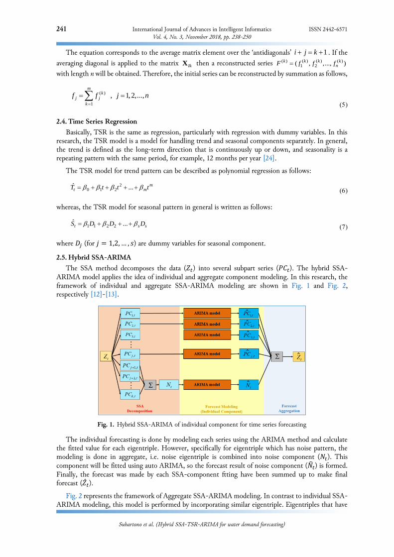
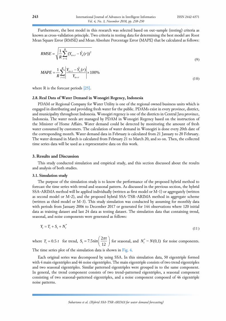
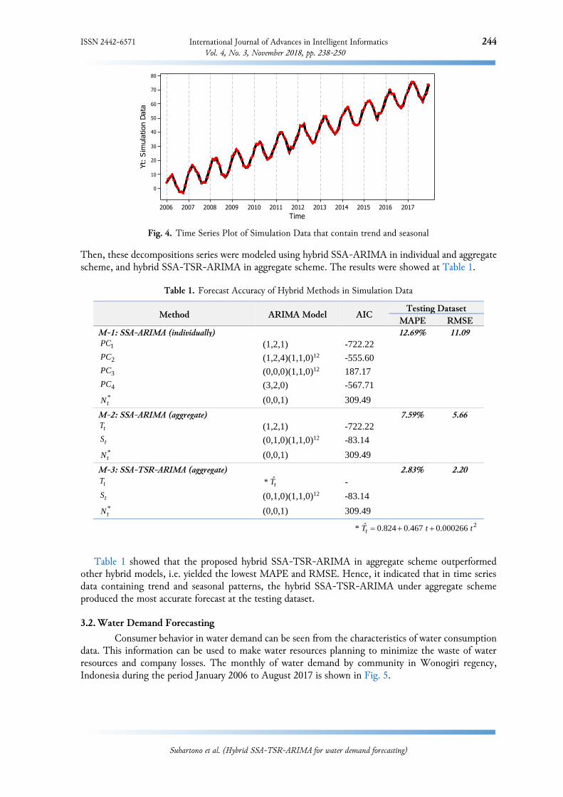
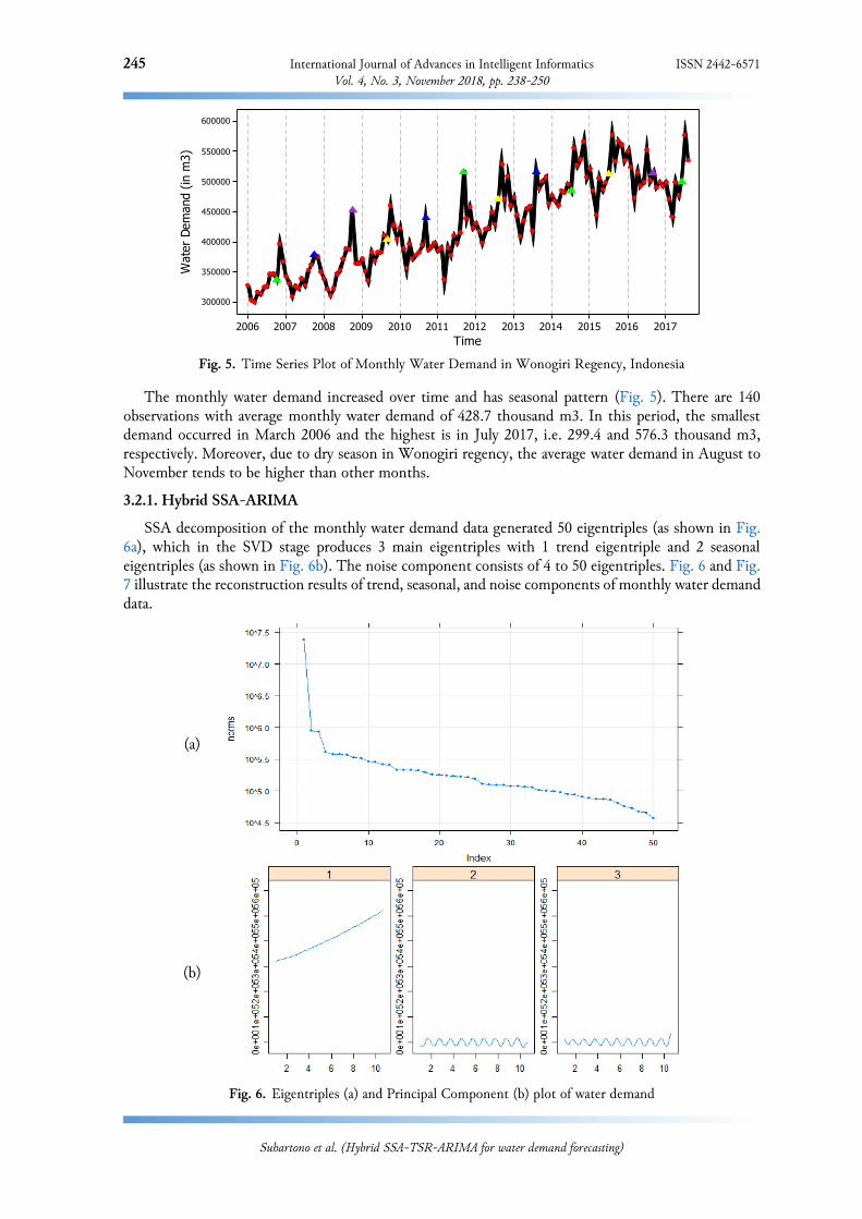
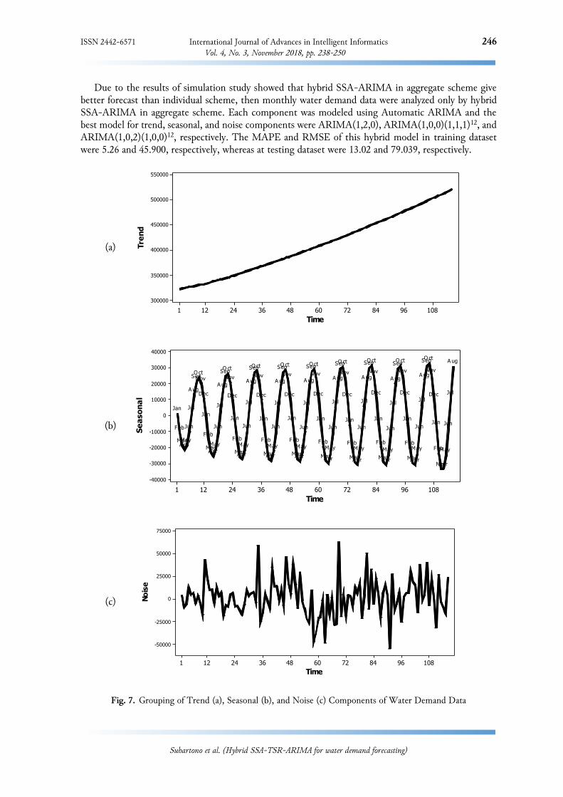
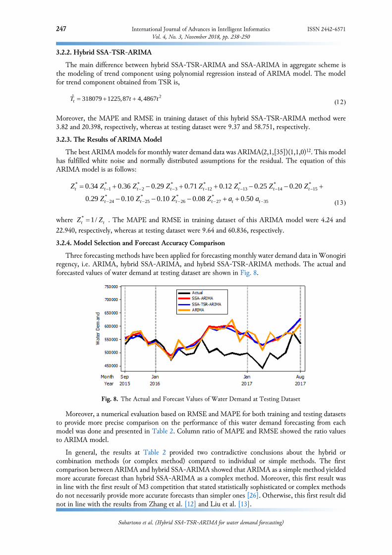
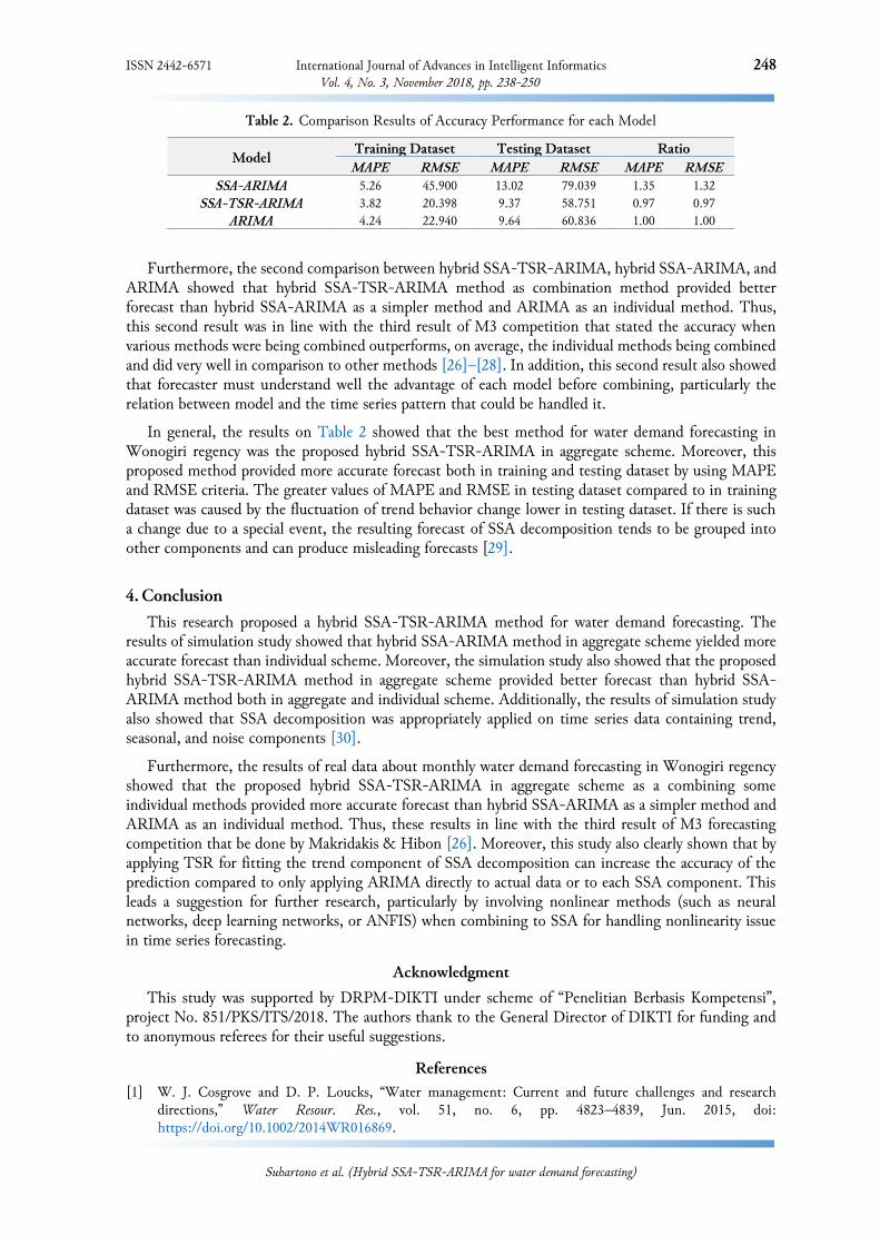


![What is Salafiyah [urdu]](https://img.pdfslide.us/doc/110x75/5593457f1a28abbb728b4737/what-is-salafiyah-urdu.jpg)


