Hybrid Simulation Theory for Continuous Beamsfaculty.ce.berkeley.edu/sanjay/ucb_semm_2014_06.pdf · Hybrid Simulation Theory for Continuous Beams By Paul L. Drazin, Sanjay Govindjee,

Report No. Structural EngineeringUCB/SEMM-2014/06 Mechanics and Materials

Hybrid Simulation TheoryforContinuous Beams

By

Paul L. Drazin, Sanjay Govindjee,andKhalid M. Mosalam

June 2014 Department of Civil and Environmental EngineeringUniversity of California, Berkeley

HYBRID SIMULATION THEORY FOR CONTINUOUS

BEAMS

Paul L. Drazin1,Sanjay Govindjee2,

and Khalid M. Mosalam2

ABSTRACT

Hybrid Simulation is an experimental technique involving the integration of a phys-

ical system and a computational system with the use of actuators and sensors. This

method has a long history in the experimental community and has been used for nearly

40 years. However, there is a distinct lack of theoretical research on the performance of

this method. Hybrid simulation experiments are performed with the implicit assump-

tion of an accurate result as long as sensor and actuator errors are minimized. However,

no theoretical results confirm this intuition nor is it understood how minimal the er-

ror should be and what the essential controlling factors are. To address this deficit in

knowledge, we consider the problem as one of tracking the trajectory of a dynamical

system in a suitably defined configuration space. In order to make progress, we further

consider a strictly theoretical hybrid system. This allows for precise definitions of errors

during a hybrid simulation. As a model system we look at an elastic beam as well as a

viscoelastic beam. In both cases we consider systems with a continuous distribution of

mass as occurs in real physical systems. Errors in the system are then tracked during

harmonic excitation using space-time L2-norms defined over the system’s configuration

space. We then present a parametric study of how magnitude and phase errors in the

control system relate to the performance of a hybrid simulation. We are able to show

sharp sensitivities to control system errors. Further, we are able to show the existence

of unacceptably high errors whenever excitations exceed the system’s first fundamental

frequency.

Keywords: hybrid system; real-time hybrid simulation; elastic beam theory;error analysis; experimental error; viscoelastic beam

BACKGROUND

Hybrid simulation is an experimental methodology in which part of a systemis tested physically and the remaining part of the system is modeled computation-ally. The two types of substructures are then interfaced. This allows for only partof the system to be constructed and tested in order for the whole system to be

1Grad. Student, Dept. of Mechanical Engineering, College of Engineering, Univ. of Califor-nia, Berkeley, Berkeley, CA 94720

2Prof., Dept. of Civil and Environmental Engineering, College of Engineering, Univ. ofCalifornia, Berkeley, Berkeley, CA 94720

1 Report No.: UCB/SEMM-2014/06

studied. The methodology allows for an economical means for the testing of largesystems subjected to dynamical loads; see e.g. Takanashi et al. 1975, Mahin andWilliams 1980, Mosalam et al. 1998. This is clearly useful for systems that aretypically too large or expensive to be fully tested and for those that contain sub-systems whose nonlinearities possess no known models. Hybrid simulation maybe categorized into two broad types: real-time hybrid simulation and pseudo-dynamic testing or simply hybrid simulation; see e.g. Schellenberg 2008. Theformer uses a laboratory system to drive the experiment in a real-time setting,typically with the use of a shaking table and other actuators which provide truedynamic loads. The latter uses a step-by-step imposition of the load where thephysical system moves quasi-statically and the mass and viscous damping char-acteristics of the system are modeled numerically. Hybrid simulation has beenmainly used as a testing method in structural mechanics, especially for earth-quake response testing; see e.g. Takanashi and Nakashima 1987. However, hybridsimulation is not exclusive to earthquake engineering and is widely applicable tosituations where it is impractical to build a complete physical system for testing;see e.g. Bursi et al. 2011.

In order to perform hybrid testing one must of course have knowledge of thegoverning equations for the part of the system to be modeled in the computer;see e.g. Mosalam and Gunay 2014. With this basic information, a simulationmethodology must be chosen and the computer interfaced to the physical part ofthe system via a collection of sensors and actuators. It is noted that the sensorsin the physical part of the system provide information to the computational partof the system regarding their current state and the actuators manipulate thephysical part of the system based on the current state of the computational partof the system. At its essence hybrid simulation involves the splitting of a systeminto two parts with the assumption that the interfacing methodology allows oneto accurately replicate the response of the system should one have decided tophysically test it in its entirety.

Most of the work on hybrid simulation has been devoted to the actual execu-tion of experiments; as this is large task in and of itself, little theoretical work hasbeen performed to verify the results that these experiments produce. There hasbeen some study of the errors associated with hybrid simulation, but in many ofthose situations, the errors studied were due to the entire experimental setup andnumerical integration, rather than the errors directly associated with a hybridsystem itself; see e.g. Shing and Mahin 1987. This paper, on the other hand,focuses solely on the theoretical performance of real-time hybrid simulation asan experimental method. This approach eliminates the errors associated withtime integration methods and focuses only on the errors that are generated bysplitting the system into a hybrid one. To make our analysis concrete, we focuson a harmonically driven simply supported beam. This system has been chosenfor its relative simplicity and the ability to analyze the solution in an analyticalform. We look at both the elastic as well as the viscoelastic cases. Further, wealways consider the case of distributed mass as occurs in real physical objects.


u(x, t)

D

∂D(a)

up(x, t)

P

uc(x, t)

C

I

(b)

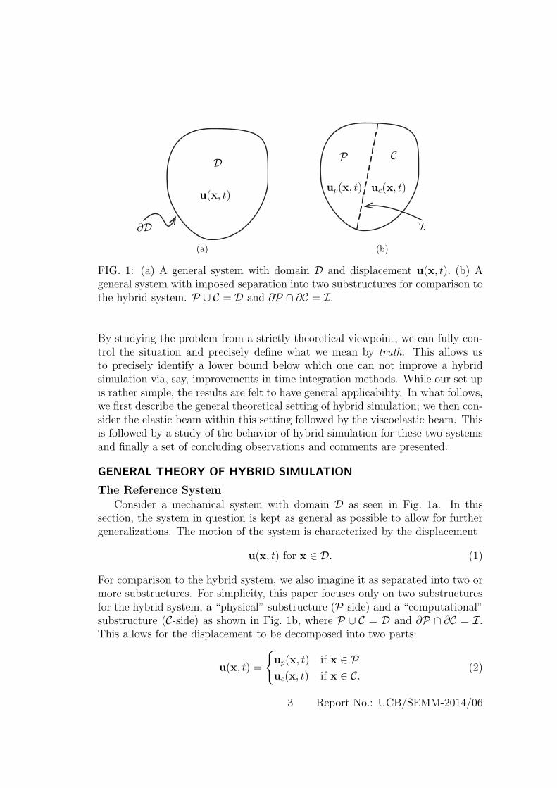
FIG. 1: (a) A general system with domain D and displacement u(x, t). (b) Ageneral system with imposed separation into two substructures for comparison tothe hybrid system. P ∪ C = D and ∂P ∩ ∂C = I.

By studying the problem from a strictly theoretical viewpoint, we can fully con-trol the situation and precisely define what we mean by truth. This allows usto precisely identify a lower bound below which one can not improve a hybridsimulation via, say, improvements in time integration methods. While our set upis rather simple, the results are felt to have general applicability. In what follows,we first describe the general theoretical setting of hybrid simulation; we then con-sider the elastic beam within this setting followed by the viscoelastic beam. Thisis followed by a study of the behavior of hybrid simulation for these two systemsand finally a set of concluding observations and comments are presented.

GENERAL THEORY OF HYBRID SIMULATION

The Reference System

Consider a mechanical system with domain D as seen in Fig. 1a. In thissection, the system in question is kept as general as possible to allow for furthergeneralizations. The motion of the system is characterized by the displacement

u(x, t) for x ∈ D. (1)

For comparison to the hybrid system, we also imagine it as separated into two ormore substructures. For simplicity, this paper focuses only on two substructuresfor the hybrid system, a “physical” substructure (P-side) and a “computational”substructure (C-side) as shown in Fig. 1b, where P ∪ C = D and ∂P ∩ ∂C = I.This allows for the displacement to be decomposed into two parts:

u(x, t) =

up(x, t) if x ∈ Puc(x, t) if x ∈ C.

(2)


up(x, t)

P

uc(x, t)

C

∂D ∩ ∂P

g(•)c ∂D ∩ ∂C

Ic = I ∩ ∂CIp = I ∩ ∂P

g(•)p

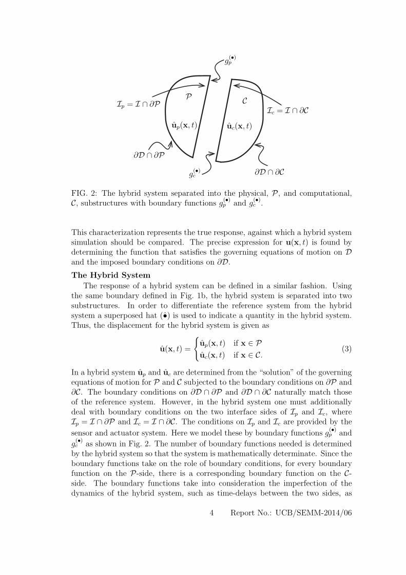
FIG. 2: The hybrid system separated into the physical, P, and computational,C, substructures with boundary functions g

(•)p and g

(•)c .

This characterization represents the true response, against which a hybrid systemsimulation should be compared. The precise expression for u(x, t) is found bydetermining the function that satisfies the governing equations of motion on Dand the imposed boundary conditions on ∂D.

The Hybrid System

The response of a hybrid system can be defined in a similar fashion. Usingthe same boundary defined in Fig. 1b, the hybrid system is separated into twosubstructures. In order to differentiate the reference system from the hybridsystem a superposed hat (•) is used to indicate a quantity in the hybrid system.Thus, the displacement for the hybrid system is given as

u(x, t) =

up(x, t) if x ∈ Puc(x, t) if x ∈ C.

(3)

In a hybrid system up and uc are determined from the “solution” of the governingequations of motion for P and C subjected to the boundary conditions on ∂P and∂C. The boundary conditions on ∂D ∩ ∂P and ∂D ∩ ∂C naturally match thoseof the reference system. However, in the hybrid system one must additionallydeal with boundary conditions on the two interface sides of Ip and Ic, whereIp = I ∩ ∂P and Ic = I ∩ ∂C. The conditions on Ip and Ic are provided by the

sensor and actuator system. Here we model these by boundary functions g(•)p and

g(•)c as shown in Fig. 2. The number of boundary functions needed is determinedby the hybrid system so that the system is mathematically determinate. Since theboundary functions take on the role of boundary conditions, for every boundaryfunction on the P-side, there is a corresponding boundary function on the C-side. The boundary functions take into consideration the imperfection of thedynamics of the hybrid system, such as time-delays between the two sides, as


well as the magnitude of tracking errors in the motion and traction as needed bythe system at hand. In the analysis, we formulate the correspondence betweenrelated boundary functions by the relation

D[uc]∣

∣

∣

Ic

= E D[up]∣

∣

∣

Ip

, (4)

where D[•] is an operator that generates the necessary boundary functions atthe interface from the displacements u(•) and E is an error operator that appliesdifferent error parameters to the different boundary functions created by D[•].Later in this paper, we employ a simple magnitude and phase error model forE. This allows us to study the effects of a wide variety of hybrid system errors.These types of errors are chosen due to their direct correlation to experimentalsystems; see e.g. Shing and Mahin 1987 or Ahmadizadeh et al. 2008.

L2 Space and Hybrid Simulation Error

With the above notation in hand, let us consider in further detail how one canunderstand hybrid simulation from a geometric point of view. Let us first definethe L2 function space as (see e.g. Johnson 2009):

L2(Ω) = v : v is defined on Ω and

∫

Ω

v2dx < ∞, (5)

where Ω is a bounded domain in R3. Using this definition we have

u ∈ L2(D). (6)

The restriction of u onto C is denoted as

uc ∈ L2(C) (7)

and similarly for the restriction of u onto P:

up ∈ L2(P). (8)

The same applies for the (•) quantities. We note that

L2(D) = L2(C)× L2(P). (9)

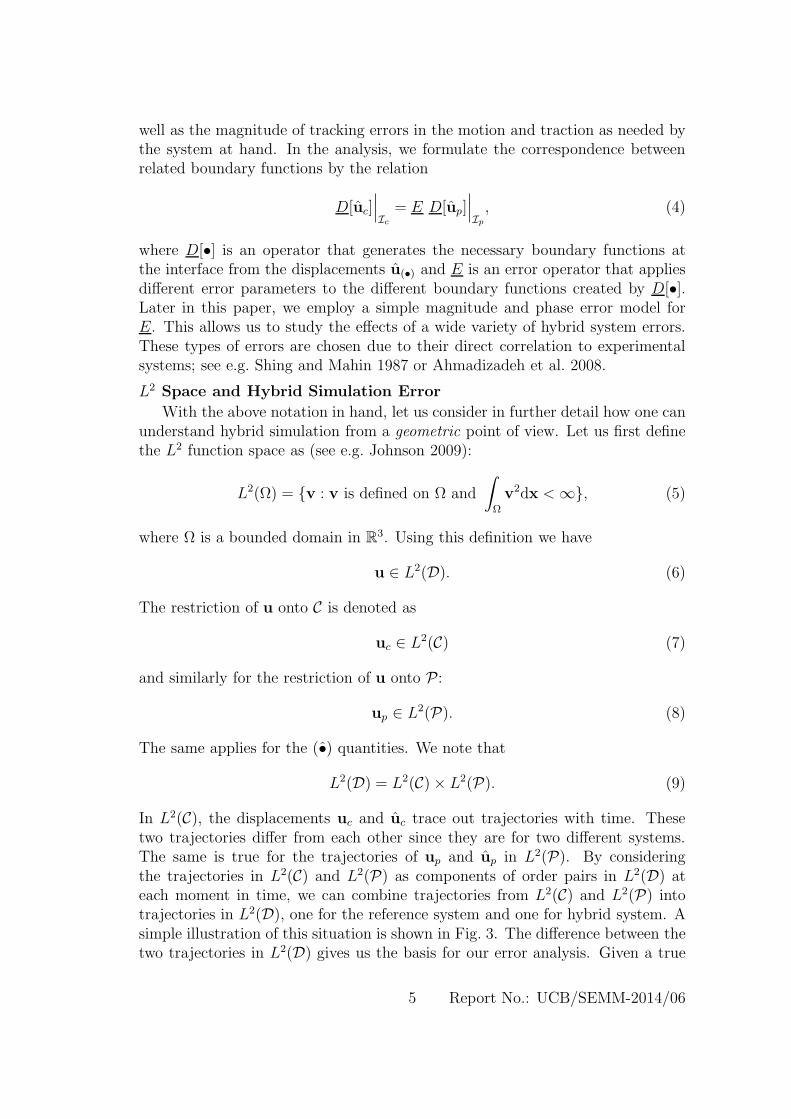
In L2(C), the displacements uc and uc trace out trajectories with time. Thesetwo trajectories differ from each other since they are for two different systems.The same is true for the trajectories of up and up in L2(P). By consideringthe trajectories in L2(C) and L2(P) as components of order pairs in L2(D) ateach moment in time, we can combine trajectories from L2(C) and L2(P) intotrajectories in L2(D), one for the reference system and one for hybrid system. Asimple illustration of this situation is shown in Fig. 3. The difference between thetwo trajectories in L2(D) gives us the basis for our error analysis. Given a true


Reference

Hybrid

L2(C)

L2(P)

u(x, t1)− u(x, t1)

u(x, t2)− u(x, t2)

FIG. 3: A schematic illustration of a possible L2(D) space with trajectories forthe reference and hybrid systems from time t = t1 to time t = t2 showing thedifference between the two trajectories.

solution u and a hybrid solution u, we measure error using a space-time L2-normin the form of (10); see e.g. Johnson 2009:

||e|| =

T∫

0

∫

D

∣

∣

∣u(x, t)− u(x, t)

∣

∣

∣

2

dxdt

1/2

, (10)

where T is the period of the harmonic excitation on the system and D is thecomplete domain of the system. This allows for a measurement of the absoluteerror between the reference system and the hybrid system over the domain of themechanical system and over the period of the harmonic excitation.

APPLICATION TO THE ELASTIC BEAM

The foregoing set-up is now applied to a continuous beam, where we haveaccess to exact analytical solutions for an intact reference system and for a hybrid(decomposed) system defined over P and C.Reference System

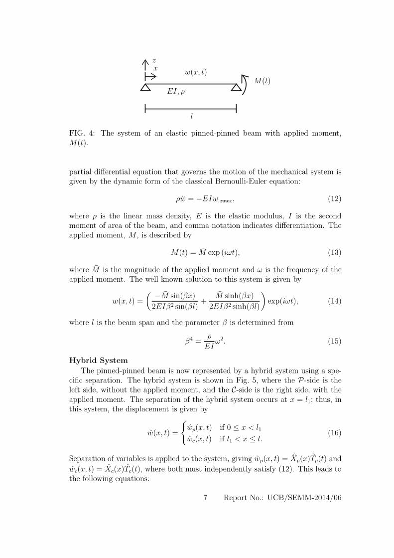
Our reference system is an elastic, homogeneous beam pinned on both endswith a harmonic moment applied to one end. A diagram of the mechanical systemis shown in Fig. 4. In this case the displacement can be decomposed as shownin (11):

w = w(x, t)ez, (11)

where ez represents the unit vector in the z-direction as indicated in Fig. 4. Inwhat follows, the vector form is ignored, and only w(x, t) is considered. The


xz

M(t)w(x, t)

l

EI, ρ

FIG. 4: The system of an elastic pinned-pinned beam with applied moment,M(t).

partial differential equation that governs the motion of the mechanical system isgiven by the dynamic form of the classical Bernoulli-Euler equation:

ρw = −EIw,xxxx, (12)

where ρ is the linear mass density, E is the elastic modulus, I is the secondmoment of area of the beam, and comma notation indicates differentiation. Theapplied moment, M , is described by

M(t) = M exp (iωt), (13)

where M is the magnitude of the applied moment and ω is the frequency of theapplied moment. The well-known solution to this system is given by

w(x, t) =

( −M sin(βx)

2EIβ2 sin(βl)+

M sinh(βx)

2EIβ2 sinh(βl)

)

exp(iωt), (14)

where l is the beam span and the parameter β is determined from

β4 =ρ

EIω2. (15)

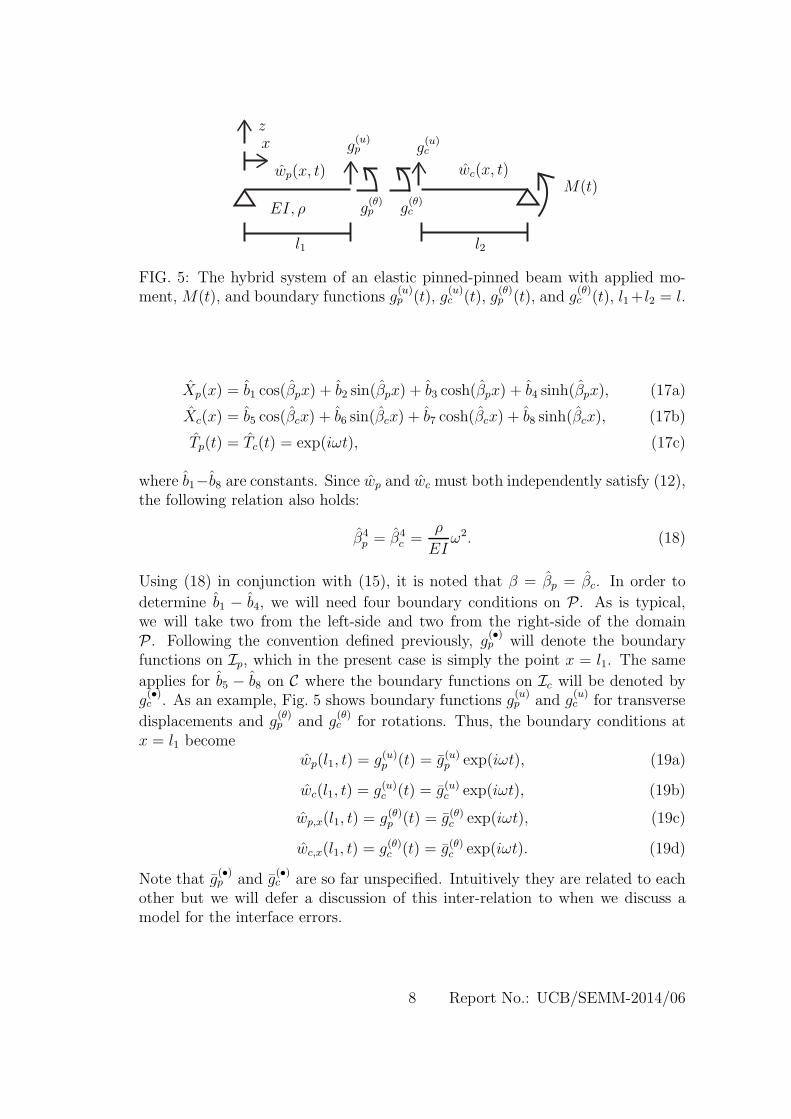
Hybrid System

The pinned-pinned beam is now represented by a hybrid system using a spe-cific separation. The hybrid system is shown in Fig. 5, where the P-side is theleft side, without the applied moment, and the C-side is the right side, with theapplied moment. The separation of the hybrid system occurs at x = l1; thus, inthis system, the displacement is given by

w(x, t) =

wp(x, t) if 0 ≤ x < l1

wc(x, t) if l1 < x ≤ l.(16)

Separation of variables is applied to the system, giving wp(x, t) = Xp(x)Tp(t) and

wc(x, t) = Xc(x)Tc(t), where both must independently satisfy (12). This leads tothe following equations:


xz

M(t)wp(x, t)

l1

EI, ρ

g(u)p g

(u)c

wc(x, t)

l2

g(θ)p g

(θ)c

FIG. 5: The hybrid system of an elastic pinned-pinned beam with applied mo-ment, M(t), and boundary functions g

(u)p (t), g

(u)c (t), g

(θ)p (t), and g

(θ)c (t), l1+ l2 = l.

Xp(x) = b1 cos(βpx) + b2 sin(βpx) + b3 cosh(βpx) + b4 sinh(βpx), (17a)

Xc(x) = b5 cos(βcx) + b6 sin(βcx) + b7 cosh(βcx) + b8 sinh(βcx), (17b)

Tp(t) = Tc(t) = exp(iωt), (17c)

where b1−b8 are constants. Since wp and wc must both independently satisfy (12),the following relation also holds:

β4p = β4

c =ρ

EIω2. (18)

Using (18) in conjunction with (15), it is noted that β = βp = βc. In order to

determine b1 − b4, we will need four boundary conditions on P. As is typical,we will take two from the left-side and two from the right-side of the domainP. Following the convention defined previously, g

(•)p will denote the boundary

functions on Ip, which in the present case is simply the point x = l1. The same

applies for b5 − b8 on C where the boundary functions on Ic will be denoted byg(•)c . As an example, Fig. 5 shows boundary functions g

(u)p and g

(u)c for transverse

displacements and g(θ)p and g

(θ)c for rotations. Thus, the boundary conditions at

x = l1 becomewp(l1, t) = g(u)p (t) = g(u)p exp(iωt), (19a)

wc(l1, t) = g(u)c (t) = g(u)c exp(iωt), (19b)

wp,x(l1, t) = g(θ)p (t) = g(θ)c exp(iωt), (19c)

wc,x(l1, t) = g(θ)c (t) = g(θ)c exp(iωt). (19d)

Note that g(•)p and g

(•)c are so far unspecified. Intuitively they are related to each

other but we will defer a discussion of this inter-relation to when we discuss amodel for the interface errors.


Solving for b1−b8, while employing the requisite boundary conditions at x = 0,x = l, Ip, and Ic, gives

wp(x, t) =g(u)p D2(βl1, βx)− g

(θ)p

βD3(βl1, βx)

D2(βl1, βl1)exp(iωt), (20)

wc(x, t) =

(

M

2EIβ2

(

A1(βl2)B1 (β(x− l1))−B1(βl2)A1 (β(x− l1)))

−g(u)c D2(βl2, β(x− l)) +g(θ)c

βD3(β(x− l), βl2)

)

exp(iωt)

D2(βl2, βl2), (21)

whereA1(x) = sin(x)− sinh(x), (22a)

B1(x) = cosh(x)− cos(x), (22b)

D2(x, y) = cosh(x) sin(y)− cos(x) sinh(y), (22c)

D3(x, y) = sinh(x) sin(y)− sin(x) sinh(y). (22d)

Non-Dimensionalization and Determination of g(•)p and g

(•)c

To further the analysis, one needs to determine the so far unspecified boundaryfunctions. In this regard, it is advantageous to non-dimensionalize the equationsas well as to express the reference solution in the same format as the hybridsolution. For the latter point, an examination of (14) and (22) shows that onecan write the reference solution as

w(x, t) =MD3(βx, βl)

2EIβ2P1(βl)exp(iωt), (23)

whereP1(x) = sin(x) sinh(x). (24)

In order to non-dimensionalize (20), (21), and (23), we introduce the followingnon-dimensional quantities:

η =w

l, ηp =

wp

l, ηc =

wc

l, y =

x

l, (25a)

µ =Ml

EI, (25b)

ω1 =

√

EI

ρ

π2

l2, Ω =

ω

ω1, τ = ω1t, (25c)

κ = βl = π√Ω, (25d)

G(u)p =

g(u)p

l, G(u)

c =g(u)c

l, G(θ)

p = g(θ)p , G(θ)c = g(θ)c , (25e)


L1 =l1l, L2 = 1− L1, (25f)

where ω1 is the lowest resonant frequency of the pinned-pinned beam; see e.g. Tongue2002. Thus (20), (21), and (23) become

η(y, τ) =µD3(κy, κ)

2κ2P1(κ)exp(iΩτ), (26)

ηp(y, τ) =G

(u)p D2(κL1, κy)− G

(θ)p

κD3(κL1, κy)

D2(κL1, κL1)exp(iΩτ), (27)

ηc(y, τ) =

(

µ

2κ2

(

A1(κL2)B1(κ(y − L1))− B1(κL2)A1(κ(y − L1)))

−G(u)c D2(κL2, κ(y − 1)) +

G(θ)c

κD3(κ(y − 1), κL2)

)

exp(iΩτ)

D2(κL2, κL2).

(28)

For the rest of this section, unless stated otherwise, all new variables or quantitiesare assumed to be dimensionless.

To complete the system of equations, G(•)p and G

(•)c need to be determined.

The conditions to determine G(•)P and G

(•)c come from the characteristics of the

sensor and actuator control system. As a simple model, we assume that the hybridsystem produces a magnitude and phase error in the corresponding displacements,rotations, bending moments, and shear forces across the interface of the hybridsystem. Using the notation introduced in (4), we write D[•] as

D[•] =

•∂•∂y

∂2•

∂y2

∂3•

∂y3

, (29)

and express E as a 4 × 4 matrix with (1 + ǫ(•)) exp(iΩd(•)) on the diagonal andzeros everywhere else. Here, ǫ(•) are the magnitude of the tracking errors for thedisplacement, rotation, bending moment, and shear force at the interface and d(•)are the tracking error time delays of the displacement, rotation, bending moment,and shear force. ǫ(•) and d(•) model the interface error in the hybrid system at I.Using this model gives

ηc(L1, τ) = ηp(L1, τ)(1 + ǫu) exp(iΩdu), (30a)

ηc,y(L1, τ) = ηp,y(L1, τ)(1 + ǫθ) exp(iΩdθ), (30b)

ηc,yy(L1, τ) = ηp,yy(L1, τ)(1 + ǫM ) exp(iΩdM ), (30c)


ηc,yyy(L1, τ) = ηp,yyy(L1, τ)(1 + ǫV ) exp(iΩdV ). (30d)

Equations (30) can be used to analytically solve for G(•)p and G

(•)c and thus com-

plete the solution; see Drazin 2013. Note that this error model can be made moresophisticated but suffices to understand a number of features of hybrid systems.

APPLICATION TO THE VISCOELASTIC BEAM

The same pinned-pinned beam model used previously is adopted for the vis-coelastic case. For this purpose we introduce the complex elastic modulus:

E∗ = E ′ + iE ′′, (31)

where E ′ is the storage modulus, E ′′ is the loss modulus, and i =√−1 is the

imaginary unit; see e.g. Ferry 1970. To be concrete, we will employ the standard3-parameter Maxwell model for a linear viscoelastic solid (the so-called standardlinear solid); see e.g. Tschoegl 1989. In this case,

E ′ = E∞ +ω2t2r

1 + ω2t2r(E0 −E∞), (32a)

E ′′ =ωtr

1 + ω2t2r(E0 −E∞), (32b)

where E0 is the instantaneous modulus and E∞ is the equilibrium modulus. Therelaxation time, tr, is given by

tr =1

ω1ζ. (33)

The parameter ζ is the non-dimensional damping frequency, which determinesthe location of the damping peak in the frequency domain. Since E∗ is complex,it can be expressed in polar form by

E∗ = |E∗| exp(iδ), (34a)

|E∗| =√E ′2 + E ′′2, (34b)

δ = tan−1

(

E ′′

E ′

)

. (34c)

Using this form of the complex elastic modulus, (15) becomes

ρω2 = |E∗|I exp(iδ)β4. (35)

Since ω, |E∗|, I, and ρ are real values, β must be complex. Solving for β resultsin

β = 4

√

ρ

|E∗|I√ω exp

(−iδ

4

)

. (36)

The solution for the reference system now reads

w(x, t) =

(−M exp(−iδ) sin(βx)

2|E∗|Iβ2 sin(βl)+

M exp(−iδ) sinh(βx)

2|E∗|Iβ2 sinh(βl)

)

exp(iωt). (37)


The non-dimensionalization of (37) and the application of the functions definedby (22) and (24) lead to the same relation given by (26), where all values havethe same definitions as before except

κ = βl = π√Ωexp

(−iδ

4

)

, (38a)

and

µ =Ml exp(−iδ)

|E∗|I . (38b)

Likewise, (27) and (28) hold for the viscoelastic pinned-pinned hybrid beam case,using the new definitions of κ and µ.

ANALYSIS OF THE HYBRID SYSTEMS

Having analytic expressions for the response of the reference systems and thehybrid systems, we are now in a position to examine the intrinsic errors associatedwith hybrid simulation using our interface model. Error in hybrid simulation fora given loading and a given set of ǫ(•) and d(•) will be defined using the non-dimensionalized response functions as

e(y, τ) = η(y, τ)− η(y, τ). (39)

For analysis purposes we will examine the L2-norm of this quantity defined by

||ep||2 =T∫

0

L1∫

0

(

Re(

η(y, τ)− ηp(y, τ))

)2

dydτ, (40a)

||ec||2 =T∫

0

1∫

L1

(

Re(

η(y, τ)− ηc(y, τ))

)2

dydτ, (40b)

||e|| =√

||ep||2 + ||ec||2, (40c)

where T is the non-dimensional period of the applied bending moment, meaningthat it changes with Ω and Re(•) is the real part of (•). The functions η(y, τ),ηp(y, τ), and ηc(y, τ) are from (26), (27), and (28), respectively. Due to the com-plexity of developing an analytic form for these norms, we choose to numericallyevaluate the integrals appearing in the norm expressions with a high order adap-tive quadrature rule to at least an absolute error of 10−10 and at least a relativeerror of 10−6.


−5

0

5

x 10−5

−5

0

5

x 10−5

0 0.2 0.4 0.6 0.8 1−2

0

2x 10

−18

y

η(y,τ)

η(y,τ)

e(y,τ)

Ω = 2.3, L1 = 0.35, τ = 0

(a)

−5

0

5

x 10−5

−5

0

5

x 10−5

0 0.2 0.4 0.6 0.8 1

−2

0

2

x 10−5

y

ǫu = 0.1

(b)

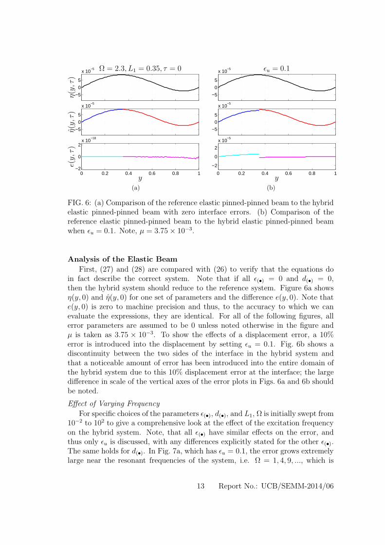
FIG. 6: (a) Comparison of the reference elastic pinned-pinned beam to the hybridelastic pinned-pinned beam with zero interface errors. (b) Comparison of thereference elastic pinned-pinned beam to the hybrid elastic pinned-pinned beamwhen ǫu = 0.1. Note, µ = 3.75× 10−3.

Analysis of the Elastic Beam

First, (27) and (28) are compared with (26) to verify that the equations doin fact describe the correct system. Note that if all ǫ(•) = 0 and d(•) = 0,then the hybrid system should reduce to the reference system. Figure 6a showsη(y, 0) and η(y, 0) for one set of parameters and the difference e(y, 0). Note thate(y, 0) is zero to machine precision and thus, to the accuracy to which we canevaluate the expressions, they are identical. For all of the following figures, allerror parameters are assumed to be 0 unless noted otherwise in the figure andµ is taken as 3.75 × 10−3. To show the effects of a displacement error, a 10%error is introduced into the displacement by setting ǫu = 0.1. Fig. 6b shows adiscontinuity between the two sides of the interface in the hybrid system andthat a noticeable amount of error has been introduced into the entire domain ofthe hybrid system due to this 10% displacement error at the interface; the largedifference in scale of the vertical axes of the error plots in Figs. 6a and 6b shouldbe noted.

Effect of Varying Frequency

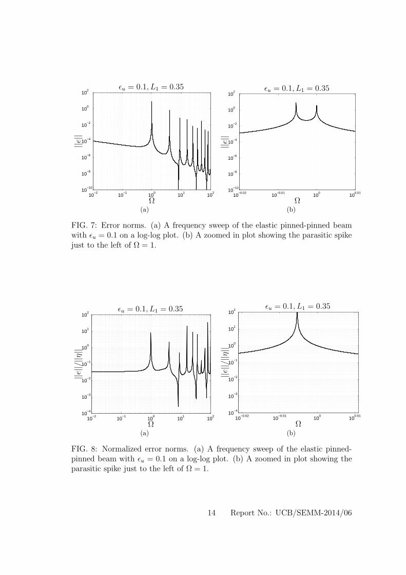
For specific choices of the parameters ǫ(•), d(•), and L1, Ω is initially swept from10−2 to 102 to give a comprehensive look at the effect of the excitation frequencyon the hybrid system. Note, that all ǫ(•) have similar effects on the error, andthus only ǫu is discussed, with any differences explicitly stated for the other ǫ(•).The same holds for d(•). In Fig. 7a, which has ǫu = 0.1, the error grows extremelylarge near the resonant frequencies of the system, i.e. Ω = 1, 4, 9, ..., which is


10−2

10−1

100

101

102

10−10

10−8

10−6

10−4

10−2

100

102

Ω

||e||

ǫu = 0.1, L1 = 0.35

(a)

10−0.02

10−0.01

100

100.01

10−10

10−8

10−6

10−4

10−2

100

102

Ω

||e||

ǫu = 0.1, L1 = 0.35

(b)

FIG. 7: Error norms. (a) A frequency sweep of the elastic pinned-pinned beamwith ǫu = 0.1 on a log-log plot. (b) A zoomed in plot showing the parasitic spikejust to the left of Ω = 1.

10−2

10−1

100

101

102

10−4

10−3

10−2

10−1

100

101

102

Ω

||e||/

||η||

ǫu = 0.1, L1 = 0.35

(a)

10−0.02

10−0.01

100

100.01

10−4

10−3

10−2

10−1

100

101

102

Ω

||e||/

||η||

ǫu = 0.1, L1 = 0.35

(b)

FIG. 8: Normalized error norms. (a) A frequency sweep of the elastic pinned-pinned beam with ǫu = 0.1 on a log-log plot. (b) A zoomed in plot showing theparasitic spike just to the left of Ω = 1.


10−2

10−1

100

10−4

10−3

10−2

10−1

100

101

102

Ω

||e||/

||η||

du = 0.1, L1 = 0.35

(a)

10−2

10−1

100

10−4

10−3

10−2

10−1

100

101

102

Ω

||e||/

||η||

ǫu = 0.1, du = 0.1, L1 = 0.35

(b)

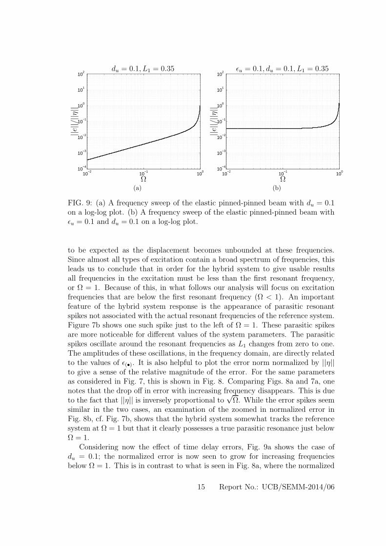
FIG. 9: (a) A frequency sweep of the elastic pinned-pinned beam with du = 0.1on a log-log plot. (b) A frequency sweep of the elastic pinned-pinned beam withǫu = 0.1 and du = 0.1 on a log-log plot.

to be expected as the displacement becomes unbounded at these frequencies.Since almost all types of excitation contain a broad spectrum of frequencies, thisleads us to conclude that in order for the hybrid system to give usable resultsall frequencies in the excitation must be less than the first resonant frequency,or Ω = 1. Because of this, in what follows our analysis will focus on excitationfrequencies that are below the first resonant frequency (Ω < 1). An importantfeature of the hybrid system response is the appearance of parasitic resonantspikes not associated with the actual resonant frequencies of the reference system.Figure 7b shows one such spike just to the left of Ω = 1. These parasitic spikesare more noticeable for different values of the system parameters. The parasiticspikes oscillate around the resonant frequencies as L1 changes from zero to one.The amplitudes of these oscillations, in the frequency domain, are directly relatedto the values of ǫ(•). It is also helpful to plot the error norm normalized by ||η||to give a sense of the relative magnitude of the error. For the same parametersas considered in Fig. 7, this is shown in Fig. 8. Comparing Figs. 8a and 7a, onenotes that the drop off in error with increasing frequency disappears. This is dueto the fact that ||η|| is inversely proportional to

√Ω. While the error spikes seem

similar in the two cases, an examination of the zoomed in normalized error inFig. 8b, cf. Fig. 7b, shows that the hybrid system somewhat tracks the referencesystem at Ω = 1 but that it clearly possesses a true parasitic resonance just belowΩ = 1.

Considering now the effect of time delay errors, Fig. 9a shows the case ofdu = 0.1; the normalized error is now seen to grow for increasing frequenciesbelow Ω = 1. This is in contrast to what is seen in Fig. 8a, where the normalized


−0.5 0 0.510

−4

10−3

10−2

10−1

100

101

102

ǫu

||e||/

||η||

Ω = 0.8, L1 = 0.35

(a)

0 2 4 6 810

−4

10−3

10−2

10−1

100

101

102

du

||e||/

||η||

Ω = 0.8, L1 = 0.35

(b)

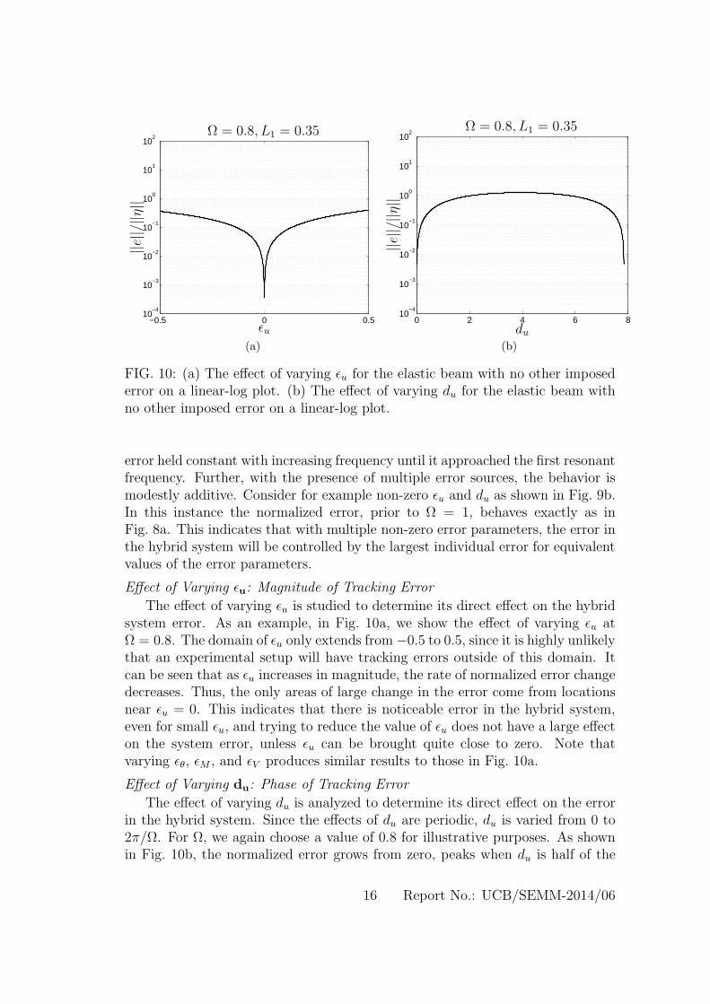
FIG. 10: (a) The effect of varying ǫu for the elastic beam with no other imposederror on a linear-log plot. (b) The effect of varying du for the elastic beam withno other imposed error on a linear-log plot.

error held constant with increasing frequency until it approached the first resonantfrequency. Further, with the presence of multiple error sources, the behavior ismodestly additive. Consider for example non-zero ǫu and du as shown in Fig. 9b.In this instance the normalized error, prior to Ω = 1, behaves exactly as inFig. 8a. This indicates that with multiple non-zero error parameters, the error inthe hybrid system will be controlled by the largest individual error for equivalentvalues of the error parameters.

Effect of Varying ǫu: Magnitude of Tracking Error

The effect of varying ǫu is studied to determine its direct effect on the hybridsystem error. As an example, in Fig. 10a, we show the effect of varying ǫu atΩ = 0.8. The domain of ǫu only extends from−0.5 to 0.5, since it is highly unlikelythat an experimental setup will have tracking errors outside of this domain. Itcan be seen that as ǫu increases in magnitude, the rate of normalized error changedecreases. Thus, the only areas of large change in the error come from locationsnear ǫu = 0. This indicates that there is noticeable error in the hybrid system,even for small ǫu, and trying to reduce the value of ǫu does not have a large effecton the system error, unless ǫu can be brought quite close to zero. Note thatvarying ǫθ, ǫM , and ǫV produces similar results to those in Fig. 10a.

Effect of Varying du: Phase of Tracking Error

The effect of varying du is analyzed to determine its direct effect on the errorin the hybrid system. Since the effects of du are periodic, du is varied from 0 to2π/Ω. For Ω, we again choose a value of 0.8 for illustrative purposes. As shownin Fig. 10b, the normalized error grows from zero, peaks when du is half of the


−1

0

1

x 10−5

−1

0

1

x 10−5

0 0.2 0.4 0.6 0.8 1

−5

0

5

x 10−19

y

η(y,τ)

η(y,τ)

e(y,τ)

Ω = 4, L1 = 0.35, τ = 0, ζ = 2

FIG. 11: Comparison of the reference viscoelastic pinned-pinned beam to thehybrid viscoelastic pinned-pinned beam with no imposed error.

period, and then falls when du is equal to a period. Note that varying dθ, dM ,and dV produces similar results as in Fig. 10b.

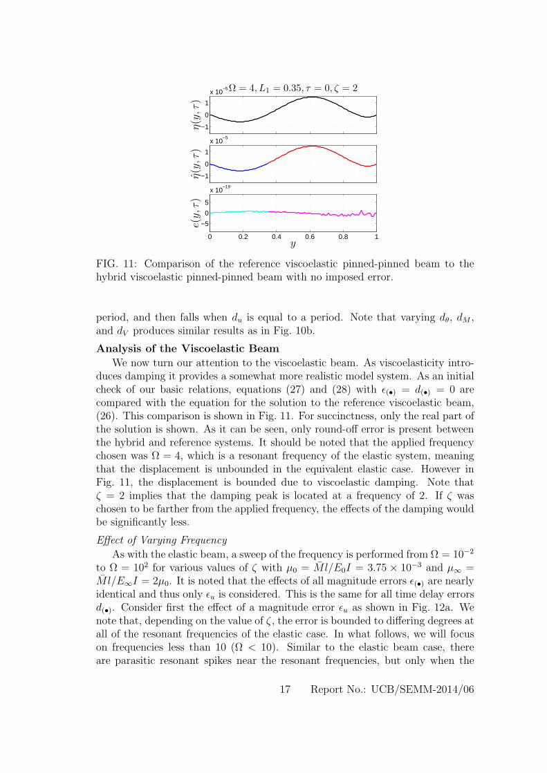
Analysis of the Viscoelastic Beam

We now turn our attention to the viscoelastic beam. As viscoelasticity intro-duces damping it provides a somewhat more realistic model system. As an initialcheck of our basic relations, equations (27) and (28) with ǫ(•) = d(•) = 0 arecompared with the equation for the solution to the reference viscoelastic beam,(26). This comparison is shown in Fig. 11. For succinctness, only the real part ofthe solution is shown. As it can be seen, only round-off error is present betweenthe hybrid and reference systems. It should be noted that the applied frequencychosen was Ω = 4, which is a resonant frequency of the elastic system, meaningthat the displacement is unbounded in the equivalent elastic case. However inFig. 11, the displacement is bounded due to viscoelastic damping. Note thatζ = 2 implies that the damping peak is located at a frequency of 2. If ζ waschosen to be farther from the applied frequency, the effects of the damping wouldbe significantly less.

Effect of Varying Frequency

As with the elastic beam, a sweep of the frequency is performed from Ω = 10−2

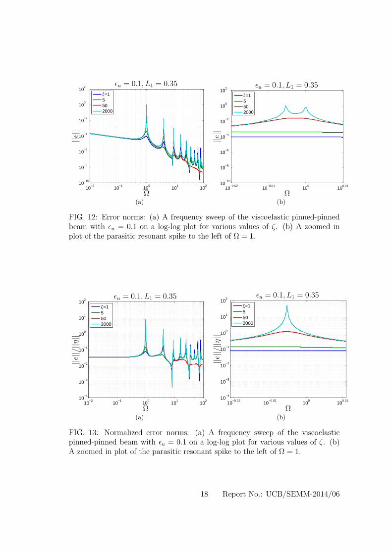
to Ω = 102 for various values of ζ with µ0 = Ml/E0I = 3.75 × 10−3 and µ∞ =Ml/E∞I = 2µ0. It is noted that the effects of all magnitude errors ǫ(•) are nearlyidentical and thus only ǫu is considered. This is the same for all time delay errorsd(•). Consider first the effect of a magnitude error ǫu as shown in Fig. 12a. Wenote that, depending on the value of ζ , the error is bounded to differing degrees atall of the resonant frequencies of the elastic case. In what follows, we will focuson frequencies less than 10 (Ω < 10). Similar to the elastic beam case, thereare parasitic resonant spikes near the resonant frequencies, but only when the


10−2

10−1

100

101

102

10−10

10−8

10−6

10−4

10−2

100

102

ζ=15502000

Ω

||e||

ǫu = 0.1, L1 = 0.35

(a)

10−0.02

10−0.01

100

100.01

10−10

10−8

10−6

10−4

10−2

100

102

ζ=15502000

Ω

||e||

ǫu = 0.1, L1 = 0.35

(b)

FIG. 12: Error norms: (a) A frequency sweep of the viscoelastic pinned-pinnedbeam with ǫu = 0.1 on a log-log plot for various values of ζ . (b) A zoomed inplot of the parasitic resonant spike to the left of Ω = 1.

10−2

10−1

100

101

102

10−4

10−3

10−2

10−1

100

101

102

ζ=15502000

Ω

||e||/

||η||

ǫu = 0.1, L1 = 0.35

(a)

10−0.02

10−0.01

100

100.01

10−4

10−3

10−2

10−1

100

101

102

ζ=15502000

Ω

||e||/

||η||

ǫu = 0.1, L1 = 0.35

(b)

FIG. 13: Normalized error norms: (a) A frequency sweep of the viscoelasticpinned-pinned beam with ǫu = 0.1 on a log-log plot for various values of ζ . (b)A zoomed in plot of the parasitic resonant spike to the left of Ω = 1.


10−2

10−1

100

101

10−4

10−3

10−2

10−1

100

101

102

ζ=15502000

Ω

||e||/

||η||

du = 0.1, L1 = 0.35

(a)

10−2

10−1

100

101

10−4

10−3

10−2

10−1

100

101

102

ζ=15502000

Ω

||e||/

||η||

ǫu = 0.1, du = 0.1, L1 = 0.35

(b)

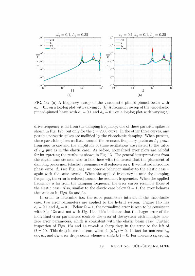
FIG. 14: (a) A frequency sweep of the viscoelastic pinned-pinned beam withdu = 0.1 on a log-log plot with varying ζ . (b) A frequency sweep of the viscoelasticpinned-pinned beam with ǫu = 0.1 and du = 0.1 on a log-log plot with varying ζ .

drive frequency is far from the damping frequency; one of these parasitic spikes isshown in Fig. 12b, but only for the ζ = 2000 curve. In the other three curves, anypossible parasitic spikes are mollified by the viscoelastic damping. When present,these parasitic spikes oscillate around the resonant frequency peaks as L1 growsfrom zero to one and the amplitude of these oscillations are related to the valueof ǫ(•) just as in the elastic case. As before, normalized error plots are helpfulfor interpreting the results as shown in Fig. 13. The general interpretations fromthe elastic case are seen also to hold here with the caveat that the placement ofdamping peaks near (elastic) resonances will reduce errors. If we instead introducephase error, du (see Fig. 14a), we observe behavior similar to the elastic case –again with the same caveat. When the applied frequency is near the dampingfrequency, the error is reduced around the resonant frequencies. When the appliedfrequency is far from the damping frequency, the error curves resemble those ofthe elastic case. Also, similar to the elastic case below Ω = 1, the error behavesthe same as in Figs. 8a and 9a.

In order to determine how the error parameters interact in the viscoelasticcase, two error parameters are applied to the hybrid system. Figure 14b hasǫu = 0.1 and du = 0.1. Below Ω = 1, the normalized error is seen to be consistentwith Fig. 13a and not with Fig. 14a. This indicates that the larger error of theindividual error parameters controls the error of the system with multiple non-zero error parameters, which is consistent with the elastic beam case. Furtherinspection of Figs. 12a and 14 reveals a sharp drop in the error to the left ofΩ = 10. This drop in error occurs when sin(κL1) = 0. In fact for non-zero ǫu,ǫM , du, and dM error drops occur whenever sin(κL1) = 0. For non-zero ǫθ, ǫV , dθ,


−0.5 0 0.510

−4

10−3

10−2

10−1

100

101

102

ζ=15502000

ǫu

||e||/

||η||

Ω = 0.8, L1 = 0.35

(a)

0 2 4 6 810

−4

10−3

10−2

10−1

100

101

102

ζ=15502000

du

||e||/

||η||

Ω = 0.8, L1 = 0.35

(b)

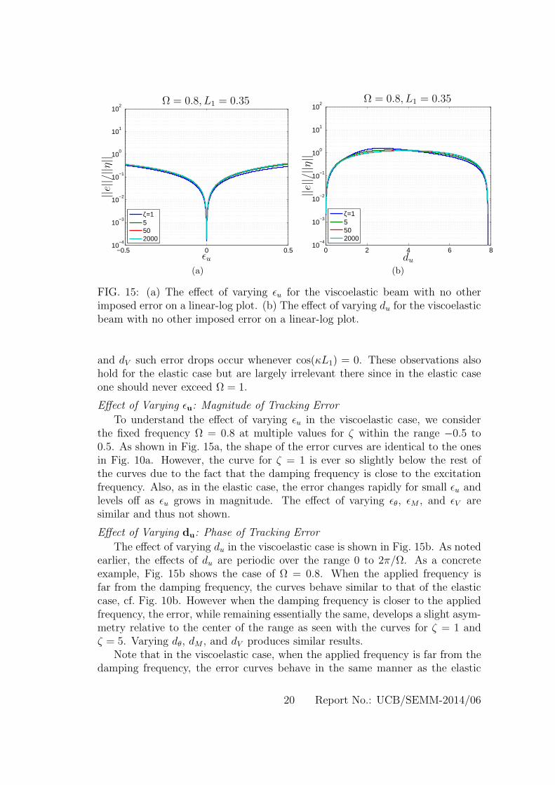
FIG. 15: (a) The effect of varying ǫu for the viscoelastic beam with no otherimposed error on a linear-log plot. (b) The effect of varying du for the viscoelasticbeam with no other imposed error on a linear-log plot.

and dV such error drops occur whenever cos(κL1) = 0. These observations alsohold for the elastic case but are largely irrelevant there since in the elastic caseone should never exceed Ω = 1.

Effect of Varying ǫu: Magnitude of Tracking Error

To understand the effect of varying ǫu in the viscoelastic case, we considerthe fixed frequency Ω = 0.8 at multiple values for ζ within the range −0.5 to0.5. As shown in Fig. 15a, the shape of the error curves are identical to the onesin Fig. 10a. However, the curve for ζ = 1 is ever so slightly below the rest ofthe curves due to the fact that the damping frequency is close to the excitationfrequency. Also, as in the elastic case, the error changes rapidly for small ǫu andlevels off as ǫu grows in magnitude. The effect of varying ǫθ, ǫM , and ǫV aresimilar and thus not shown.

Effect of Varying du: Phase of Tracking Error

The effect of varying du in the viscoelastic case is shown in Fig. 15b. As notedearlier, the effects of du are periodic over the range 0 to 2π/Ω. As a concreteexample, Fig. 15b shows the case of Ω = 0.8. When the applied frequency isfar from the damping frequency, the curves behave similar to that of the elasticcase, cf. Fig. 10b. However when the damping frequency is closer to the appliedfrequency, the error, while remaining essentially the same, develops a slight asym-metry relative to the center of the range as seen with the curves for ζ = 1 andζ = 5. Varying dθ, dM , and dV produces similar results.

Note that in the viscoelastic case, when the applied frequency is far from thedamping frequency, the error curves behave in the same manner as the elastic


case. This is to be expected, because away from the damping frequency, theviscoelastic equations approach the elastic ones. Finally, note that almost allconclusions gained from the elastic case are repeated for the viscoelastic case,except for special treatment of the parameter ζ .

CONCLUSION

The analysis in this paper demonstrates the theoretical performance of hy-brid simulation of an elastic and a viscoelastic beam for the special case wherethe only errors that are present are those associated with the hybrid (i.e. splitsystem) nature of the formulation. A harmonic excitation was applied and onlythe steady-state solution was studied. This ignores any transient response thatmay occur in experimental implementations of hybrid simulation. The resultsshow that the resonant frequencies have an outsized impact on the error of thesimulation system. Thus, in order for real-time hybrid simulation to be effectiveas a simulation technique, one must be aware of the forcing frequencies, and keepthem below the first resonant frequency for the elastic case or possibly near thedamping frequency in the viscoelastic case. The error due to ǫ(•) grows quicklyaround ǫ(•) = 0 and reaches a large error value for small ǫ(•) values. Thus, it issomewhat impractical to reduce the ǫ(•) parameters in order to reduce the errorin the system, because unless one can make the ǫ(•) values quite small, the sys-tem error does not significantly change. All of the results stated in the analysissection have also been corroborated with hybrid formulations for an elastic anda viscoelastic axially loaded bar (see Drazin 2013) as well as for a classical elas-tic Kirchhoff-Love plate; see Bakhaty et al. 2014. This indicates that there areuniversal errors that occur in hybrid simulation, even for simple one-dimensionaland two-dimensional problems. Awareness of the causes of these errors can allowfor real-time hybrid simulations to be conducted in a way that reduces or evenprevents these errors.

In this paper it was assumed that ǫ(•) and d(•) are constants. However, thisis not always the case, they may in fact be functions of the frequency, such thatat higher frequencies the time-delay or magnitude error may increase. To includethis effect, one could introduce models of the form

d(•) =d0

(

1 + exp(Ω0 − Ω))2 , (41)

where d0 is the maximum time delay and Ω0 is the frequency of maximum growthrate; see Bakhaty et al. 2014. Similar equations can be applied to ǫ(•). Suchmodels modify the details of the error responses; however, the trends remainfundamentally the same.

This paper considered a single homogeneous linear material that could bemodeled by (12). This is not always the case for an experimental setup of hybridsimulation. For example, many hybrid simulation setups are for many bars andbeams at the same time, each interacting with the whole system; see e.g. Mosalam


and Gunay 2014 or Gunay and Mosalam 2014. In such cases analytic responsesolutions are likely to not be available but we do not expect the observed generaltrends to be altered.

The error measure we focused on was the L2-norm of the displacement errorbut that only shows one part of error in the system. The error in the rotation,shear force, and bending moment can also be studied with the use of Sobolev-seminorms of the displacement field; see e.g. Johnson 2009. Understanding theerror in these quantities is as important as understanding the error in the dis-placement because in some situations these quantities can be of equal or evengreater importance to the structural and mechanical behavior of a system thanthe displacement; see e.g. Elkhoraibi and Mosalam 2007.

ACKNOWLEDGEMENTS

This research was financially supported by National Science Foundation AwardNumber CMMI-1153665. Any opinions, findings, and conclusions or recommen-dations expressed are those of the authors and do not necessarily reflect those ofthe National Science Foundation.


REFERENCES

Ahmadizadeh, M., Mosqueda, G., and Reinhorn, A. M. (2008). “Compensationof actuator delay and dynamics for real time hybrid structural simulation.”Earthquake Engineering and Structural Dynamics, 37, 21–42.

Bakhaty, A. A., Govindjee, S., and Mosalam, K. M. (2014). “Theoretical develop-ment of hybrid simulation applied to plate structures.” Report No. UCB-PEER-2014-02, Pacific Earthquake Engineering Research Center, Berkeley, CA.

Bursi, O. S., Jia, C., Vulcan, L., Neild, S. A., and Wagg, D. J. (2011).“Rosenbrock-based algorithms and subcycling strategies for real-time nonlin-ear substructure testing.” Earthquake Engineering and Structural Dynamics,40, 1–19.

Drazin, P. L. (2013). “Hybrid Simulation Theory Featuring Bars andBeams.” M.S. report, University of California, Berkeley, CA. URL:http://www.ce.berkeley.edu/∼sanjay/DrazinPaulMSReportFall2013.pdf.

Elkhoraibi, T. and Mosalam, K. M. (2007). “Towards error-free hybrid simulationusing mixed variables.” Earthquake Engineering and Structural Dynamics, 36,1497–1522.

Ferry, J. D. (1970). Viscoelastic Properties of Polymers. John Wiley & Sons, NewYork.

Gunay, S. and Mosalam, K. M. (2014). “Seismic performance evaluation of highvoltage disconnect switches using real-time hybrid simulation: II. parametricstudy.” Earthquake Engineering and Structural Dynamics, 43, 1223–1237.

Johnson, C. (2009). Numerical Solution of Partial Differential Equations by the

Finite Element Method. Dover Publications, Mineola, NY.Mahin, S. A. and Williams, M. E. (1980). “Computer controlled seismic perfor-mance testing.” Dynamic Response of Structures: Experimentation, Observa-

tion, Prediction and Control, American Society of Civil Engineers.Mosalam, K. M. and Gunay, S. (2014). “Seismic performance evaluation of highvoltage disconnect switches using real-time hybrid simulation: I. system devel-opment and validation.” Earthquake Engineering and Structural Dynamics, 43,1205–1222.

Mosalam, K. M., White, R. N., and Ayala, G. (1998). “Response of infilled framesusing pseudo-dynamic experimentation.” Earthquake Engineering and Struc-

tural Dynamics, 27, 589–608.Schellenberg, A. H. (2008). “Advanced implementation of hybrid simulation.”Ph.D. thesis, University of California, Berkeley, CA.

Shing, P. S. B. and Mahin, S. A. (1987). “Elimination of spurious higher-moderesponse in pseudodynamic tests.” Earthquake Engineering and Structural Dy-

namics, 15, 409–424.Takanashi, K. and Nakashima, M. (1987). “Japanese activities on on-line testing.”Journal of Engineering Mechanics, 113, 1014–1032.

Takanashi, K., Udagawa, K., Seki, M., Oakada, T., and Tanaka, H. (1975). “Non-linear earthquake response analysis of structures by a computer-actuator on-line system.” Bulletin of Earthquake Resistant Structure Research Center, 8.


Tongue, B. H. (2002). Principles of Vibration. Oxford University Press, NewYork.

Tschoegl, N. W. (1989). The Phenomenological Theory of Linear Viscoelastic

Behavior. Springer-Verlag, Berlin.


Documents

Hybrid Simulation Theory for Continuous Beamsfaculty.ce.berkeley.edu/sanjay/ucb_semm_2014_06.pdf · Hybrid Simulation Theory for Continuous Beams By Paul L. Drazin, Sanjay Govindjee,