Embed Size (px)
Citation preview
i
Hybrid Renewable Energy Systems for a
Dynamically Positioned Buoy
by
Robert Sean Pagliari
Bachelor of Science in Applied Science and Technology
In Nuclear Engineering Technology
2009
A thesis submitted to
Florida Institute of Technology
In partial fulfillment of the requirements for the degree of
Master of Science
In Ocean Engineering
Melbourne, Florida
December 2012

i
© Copyright 2012 Robert Sean Pagliari
All Rights Reserved
The author grants permission to make single copies ________________________

ii
We the undersigned committee hereby approve the attached thesis
Hybrid Renewable Energy Systems for a Dynamically
Positioned Buoy
by Robert Sean Pagliari
as fulfilling in part the requirements for the degree of
Master of Science in Ocean Engineering
__________________________________
S.L. Wood, Ph.D., P.E.
Ocean Engineering Program Chair and University Professor, Ocean Engineering
__________________________________
E.D. Thosteson, Ph.D., P.E.
Assistant Professor, Ocean Engineering
__________________________________
R.L. Sullivan, Ph.D., FIEEE
University Professor, Electrical and Computer Engineering
__________________________________
G.A. Maul, Ph.D.,
Professor and Department Head,
Department of Marine and Environmental Systems, College of Engineering
iii
Abstract
Hybrid Renewable Energy Systems for a Dynamically Positioned Buoy
by
Robert Sean Pagliari
Principal Advisor: S.L. Wood, Ph.D., P.E.
To ease the burdens associated with deep ocean buoy moorings, a relatively
recent technological development known as Dynamic Positioning (DP) could be
employed. This method, which is being used on some oil drilling ships and semi-
submersible platforms, provides pinpoint positioning for precision drilling and
other operations with the use of multiple, multi-axis, thrusters below the waterline
of a vessel to counter the effects of winds and ocean currents. This eliminates the
need for anchoring in deep oceans, but depending on the characteristics of the
vessel and environmental conditions, power requirements for DP tend to be quite
substantial and costly.
A theoretical design of a hybrid wind and solar energy system on an ocean
surface buoy is made for the purpose of powering a low cost, simple, dynamic
positioning system. This system was implemented on a dynamically positioned
buoy (DPB) intended for sea keeping using renewable energy sources.
iv
Some prototypes of autonomous surface vehicles have experimented with
renewable energies as a source of supplemental power, but these vehicles are
typically designed as transient surface vehicles with station keeping capability as a
secondary function.
A combination of design requirements set forth by 2004 Defense Advanced
Research Projects Agency (DARPA) solicitation number BAA04-33 and 2008
solicitation number DARPASN08-45 are used as a basis for DPB design
parameters. The aims of the DPB design thesis are to develop and test a low cost,
dynamic positioning system that will continuously maintain a 250 m watch radius
and to present a theoretical hybrid renewable energy system to power it, thereby
improving on the station keeping buoy (SKB) energy balance problem.
Global Positioning System (GPS) technology, combined with an 8-bit
embedded microcontroller and circuitry provide sufficient autonomous control
signals to independent thrusters below the waterline. These correct for position
offsets caused by sea and air currents in the open ocean.
The results of the system in a 2.5 m s-1
wind validated the feasibility of
mounting a horizontal axis wind turbine on a buoy without a necessary counter
balancing device. A hybrid wind and solar renewable energy system was designed
using [54]. The 100% power load of about 1280 total watts proved too substantial
to warrant the practicality of this renewable energy system in three out of four
simulations. One optimization, however, was able to produce an annual capacity

v
shortage of less than 1% using an assumed duty cycle of 10% at one location. Due
to pool size restrictions and ineffective tuning parameters the tested dynamic
positioning system was unsuccessful in validating the capability of continuously
maintaining a 250 m watch circle.
vi
Table of Contents
Abstract ....................................................................................................... iii
Table of Contents .......................................................................................... vi
List of Keywords ........................................................................................ viii
List of Figures ............................................................................................... ix
List of Tables............................................................................................... xii
List of Abbreviations.................................................................................. xiii
Preface .......................................................................................................... xv
Acknowledgements ..................................................................................... xvi
1 Introduction .............................................................................................. 1
1.1 Motivation .......................................................................................... 1
1.2 A Dynamically Positioned Buoy ........................................................ 2
2 Background .............................................................................................. 4
2.1 Buoy Designs ..................................................................................... 4
2.1.1 Buoy Moorings ...................................................................... 8
2.2 Oil Rigs ..................................................................................... 12
2.3 Dynamic Positioning ........................................................................ 12
2.4 Navigation, GPS and DGPS ............................................................. 14
2.5 Renewable Energy ........................................................................... 16
2.5.1 Wind Power .......................................................................... 17
2.5.2 Solar Power .......................................................................... 19
2.5.3 Energy Storage ..................................................................... 22
2.6 Similar Systems ................................................................................ 23
3 Development and Construction .............................................................. 28
3.1 Design Considerations ..................................................................... 28
3.1.1 Pre-existing Buoy Project .................................................... 30
3.2 DPB Build ........................................................................................ 33
3.3 Instrumentation and Control ............................................................ 34
3.3.1 GPS Receiver Module .......................................................... 35
3.3.2 Waypoint Tracking and Positioning .................................... 39
vii
3.3.3 PIC 18F Series Microcontroller ........................................... 44
3.3.4 Circuit Configuration ........................................................... 45
3.3.5 AndroidTM
Smart Phone ....................................................... 48
3.4 Software and Application ................................................................. 48
3.4.1 Embedded Systems and Pseudo Dynamic Positioning ........ 49
3.4.2 Remote Control and Logging Application for AndroidTM
... 51
4 Hybrid Renewable Energy System ........................................................ 55
4.1 Resources ......................................................................................... 55
4.1.1 Wind Resources ................................................................... 55
4.1.2 Solar Resources .................................................................... 57
4.2 Loads ............................................................................................ 60
4.2.1 Primary Electrical Load ....................................................... 60
4.2.2 Control System Electrical Load ........................................... 61
4.3 Hybrid Energy System Design ......................................................... 61
4.3.1 Hybrid Optimization Model for Electric Renewables
(HOMER) ............................................................................. 61
4.3.2 Simulation Results ............................................................... 68
4.3.3 Systems Integration .............................................................. 69
5 Testing ............................................................................................ 72
5.1 Tank Test .......................................................................................... 72
5.2 Field Tests ........................................................................................ 75
5.2.1 Dynamic Load, Stability and Performance .......................... 75
5.2.2 Form Drag Analysis from Dynamic Field Test.................... 82
5.2.3 Accuracy and Precision ........................................................ 86
5.2.4 Small Model Performance.................................................... 92
6 Conclusion and Further Development ................................................... 98
6.1 A Better DPB Design ....................................................................... 99
6.2 Further Development ..................................................................... 101
References .......................................................................................... 102
Appendix A .......................................................................................... 111
Appendix B .......................................................................................... 116
Appendix C .......................................................................................... 123
Appendix D .......................................................................................... 124
Appendix E .......................................................................................... 133

viii
List of Keywords
AndroidTM
Air Mass Coefficient
Differential Global Positioning System
Dynamic Positioning
Dynamically Positioned Buoy
Embedded Systems
Global Positioning System
Kalman Filter
Ocean Buoy
Ocean Energy
Peripheral Interface Controller
Persistent Ocean Surveillance
Renewable Energy
Smart Phone
Station Keeping Buoy
Solar Energy
Wave Energy
Wind Energy
Wind Turbine

ix
List of Figures
FIGURE 1 FROM [9] A) LIGHTED BUOY B) SPAR BUOY C) CAN BUOY ............................. 6
FIGURE 2 FROM [2] NDBC MOORED BUOY PROGRAM OFFSHORE METEOROLOGICAL
AND OCEANOGRAPHIC BUOY COLLECTION........................................................... 7
FIGURE 3 FROM [12] SURFACE BUOY MOORING CONFIGURATIONS A) CHAIN SLACK
MOORING B) CHAIN SLACK MOORING WITH ADDED CHAIN AND WIRE ROPE C)
CHAIN AND ELASTIC MOORING D) CHAIN AND ELASTIC MOORING WITH ADDED
LINES TO REDUCE WATCH CIRCLE E) TAUT SURFACE TRIMOOR SYSTEM F)
SUBMERGED BUOY AND A RIGID BUOYANT TETHER LINE G) SINGLE POINT
MOORING FOR A SHALLOW WATER SPAR BUOY .................................................. 10
FIGURE 4 FROM [12] A POTENTIAL FOR LOSS OF BUOY EXISTS DURING THE
DEPLOYMENT AS THE ANCHOR IS ALLOWED TO TWIST AND KINK THE MOORING
LINE................................................................................................................... 11
FIGURE 5 FROM [8] HORIZONTAL AXIS WIND TURBINE (LEFT) AND DARRIEUS TYPE
VERTICAL AXIS WIND TURBINE (RIGHT) ............................................................. 19
FIGURE 6 FROM [31] P AND N DOPED SEMI-CONDUCTOR CROSS-SECTION .................. 21
FIGURE 7 FROM [62] AUTONOMOUS MOBILE BUOY .................................................. 26
FIGURE 8 FROM [18] A SIMPLE DIAGRAM DEPICTING A ROTARY CRAFT ANALYSIS
WHERE A1 IS THE SWEPT AREA OF A WIND TURBINE, A2 IS THE SWEPT AREA OF A
PROPELLER, Ρ1 IS THE DENSITY OF AIR, Ρ2 IS THE DENSITY OF WATER, W IS WIND
SPEED AND V IS THE RESULTING WATER VELOCITY FROM THE PROPELLER ........ 28
FIGURE 9 FROM [30] PETER WORSLEY’S ROTARY CRAFT .......................................... 29
FIGURE 10 A) A YELLOW BUOY RENDERING FROM PRO-ENGINEER AND B) FINAL
YELLOW BUOY CONSTRUCTION ......................................................................... 31
FIGURE 11 A) RENDERING OF DPB FROM [54] B) FINAL DPB APPARATUS PHOTO
COURTESY OF DR. STEPHEN WOOD ................................................................... 31
FIGURE 12 REINFORCED WATERPROOF BATTERY HOUSING AND MOTOR MOUNT ....... 33
FIGURE 13 A) ALUMINUM CHANNELS TRANSFER THRUST TO DPB FRAME AND
SUPPORT THE WEIGHT OF THE HOUSINGS AND B) BOTTOM MOUNTED TROLLING
MOTORS PHOTOS COURTESY OF DR. STEPHEN WOOD ........................................ 34
FIGURE 14 A PSEUDO CARTESIAN COORDINATE SYSTEM APPLIED TO A LONGITUDINAL
VERSES LATITUDINAL GRID USED TO CALCULATE BEARING VIA BASIC
TRIGONOMETRIC FUNCTIONS. ............................................................................ 41
FIGURE 15 DPB EMBEDDED CONTROL CIRCUIT ......................................................... 46
x
FIGURE 16 DPB PRINTED CIRCUIT BOARD ................................................................. 47
FIGURE 17 DPB POWER RELAY CIRCUIT .................................................................... 47
FIGURE 18 FLOW CHART OF DPB INSTRUMENTATION AND CONTROL LOGIC ............. 51
FIGURE 19 ANDROID HOME SCREEN CONTAINING ALL APPLICATIONS ASSOCIATED
WITH DPB AND SHOCNET .................................................................................. 52
FIGURE 20 SHOCNET APPLICATION CONNECTED TO DPB AND BI-DIRECTIONAL DATA
STREAM ............................................................................................................. 54
FIGURE 21 FROM [35] AVERAGE WORLD WIND SPEEDS .............................................. 56
FIGURE 22 THE AVAILABLE WIND POWER PER SQUARE METER OF SURFACE AREA ..... 57
FIGURE 23 FROM [34] AVERAGE WORLD SOLAR IRRADIANCE .................................... 58
FIGURE 24 SOLAR PANEL CONFIGURATIONS .............................................................. 63
FIGURE 25 A POTENTIAL PLACEMENT OF TWO WIND TURBINES ................................. 64
FIGURE 26 POWER CURVE FOR SW AIR BREEZE WIND TURBINE EXPORTED FROM [54].
.......................................................................................................................... 64
FIGURE 27 LOAD INPUTS TO [54] BASED ON A 10% PROPULSIVE DUTY CYCLE ........... 66
FIGURE 28 AVERAGED MONTHLY SUSTAINED WIND DATA IMPORTED INTO [54] FROM
[2] TAKEN AT STATION 51004 ........................................................................... 67
FIGURE 29 AVERAGED MONTHLY SOLAR IRRADIANCE IMPORTED INTO [54] FROM [34]
TAKEN AT STATION 51004 ................................................................................. 67
FIGURE 30 HOMER SIMULATION RESULTS FOR DPB AT STATION 51004 BASED ON A
10% PROPULSIVE DUTY CYCLE .......................................................................... 69
FIGURE 31 HYBRID SYSTEM CONFIGURATION INPUT TO [54] ..................................... 70
FIGURE 32 DPBS ELECTRICAL CONFIGURATION LAYOUT .......................................... 71
FIGURE 33 THRUST TEST APPARATUS IN THE FIT WAVE TANK FACILITY WITH A FIXED
STRAIN GAUGE TO MEASURE OUTPUT FORCE ..................................................... 73
FIGURE 34 DC AMMETER CLAMPED TO THE POSITIVE LEAD OF THE MOTOR .............. 74
FIGURE 35 DBP DEPLOYMENT OBSERVATION IMAGE COURTESY OF DR. STEPHEN
WOOD ............................................................................................................... 77
FIGURE 36 EAU GALLIE CAUSEWAY STATIC ENVIRONMENT FIELD TEST AND CONTROL
SCHEME IMAGE COURTESY OF DR. STEPHEN WOOD .......................................... 77
FIGURE 37 EAU GALLIE CAUSEWAY DYNAMIC ENVIRONMENT FIELD TEST APPARATUS
AND CONTROL SCHEME IMAGE COURTESY OF DR. STEPHEN WOOD ................... 78
FIGURE 38 EAU GALLIE DYNAMIC ENVIRONMENT FIELD TEST SITE WITH
ENVIRONMENTAL CONDITION OVERLAYS .......................................................... 79

xi
FIGURE 39 DPB INSTRUMENTATION AND CONTROL PACKAGE USING LS20126 GPS
RECEIVER MODULE, PIC18F27J13 MICROCONTROLLER, AND RN-XV WIRELESS
TRANSCEIVER .................................................................................................... 81
FIGURE 40 EXTRAPOLATED DRAG CURVES FOR DPB ................................................. 83
FIGURE 41 DPB CROSS-SECTION MEASUREMENTS .................................................... 84
FIGURE 42 WIND TURBINE SWEPT AREA AND MOUNTING CROSS-SECTION
MEASUREMENTS ................................................................................................ 85
FIGURE 43 NGS BENCHMARK AT FT. TRUMBULL...................................................... 87
FIGURE 44 FT. TRUMBULL FIELD TEST RESULTS ........................................................ 89
FIGURE 45 EASTERN POINT BEACH FIELD TEST RESULTS .......................................... 90
FIGURE 46 VERIPOS AND C-NAV RELATIVE POSITIONS WITH LS20126 MODULE PLOT
OVERLAYS ......................................................................................................... 91
FIGURE 47 DPB SMALL MODEL WITH DIFFERENTIAL STEERING ................................. 92
FIGURE 48 APPLICATION OF THE ZEROTH ORDER KALMAN FILTER WITH INITIAL
VALUES OF 0.36 FOR R AND 1X10⁻⁴
FOR Q ......................................................... 95
FIGURE 49 FROM [45] A SATELLITE IMAGE OF SMALL MODEL TEST WITH THE
RECORDED PATH SUPERIMPOSED ....................................................................... 96
FIGURE 50 A MORE IDEAL DESIGN FOR RENEWABLE ENERGY STATION KEEPING ...... 100
FIGURE 51 FROM [44] LS20126 MODULE MONITORING SOFTWARE INCLUDING
ACCELEROMETER OUTPUT ............................................................................... 111
FIGURE 52 FROM [43] USED TO REDIRECT AND SPLIT TCP/IP PORT CONNECTIONS TO
VIRTUAL SERIAL PORT ..................................................................................... 111
FIGURE 53 FROM [50] TERMINAL SOFTWARE USED FOR SERIAL AND TCP/IP
COMMUNICATION ............................................................................................ 112
FIGURE 54 FROM [47] USED FOR DEVELOPMENT OF CONTROL SOFTWARE USING
PICC18 COMPILER .......................................................................................... 112
FIGURE 55 FROM [51] WIRELESS TETHER APPLICATION USED TO ESTABLISH A MOBILE
WLAN ............................................................................................................ 113
FIGURE 56 FROM [49] USED FOR MOBILE APPLICATION DEVELOPMENT ................... 114
FIGURE 57 FROM [54] USED FOR HYBRID ENERGY CONFIGURATION ANALYSIS ........ 115

xii
List of Tables
TABLE 1 ADDITIONAL ASVS AND OTHER SIMILAR SYSTEMS SIMILAR SYSTEMS ........ 27
TABLE 2 DPB FINAL SPECIFICATIONS ........................................................................ 32
TABLE 3 FROM [5] RMC DATA FORMAT .................................................................... 37
TABLE 4 SORTING EQUATIONS AND EXCEPTIONS USED FOR WAYPOINT TRACKING
ALGORITHM ....................................................................................................... 43
TABLE 5 FROM [6] DEVICE FEATURES FOR THE PIC18F2XJ13 (28-PIN
DEVICES) ....................................................................................................... 44
TABLE 6 A COMPARISON OF MICROCONTROLLER SELECTION CRITERIA ..................... 45
TABLE 7 FROM [32] COMMON 220W SOLAR PANELS ON THE MARKET AS OF MAY 19,
2012 .................................................................................................................. 59
TABLE 8 INSTRUMENTATION AND CONTROL SYSTEM LOADS ..................................... 61
TABLE 9 SEARCH SPACE FROM [54] ........................................................................... 65
TABLE 10 MEASURED AND CALCULATED CHARACTERISTICS OF THE DPB PROPULSION
SYSTEM ............................................................................................................. 74
TABLE 11 STATIC AND DYNAMIC ENVIRONMENTAL CONDITIONS .............................. 80
TABLE 12 CURRENT DATA......................................................................................... 80
TABLE 13 STATIC AND DYNAMIC TEST ENVIRONMENT VELOCITY DATA .................... 80

xiii
List of Abbreviations
AGM: Absorbed Glass Mat
ALDOS: Aluminum-dissolved Oxygen
ASTM: American Society for Testing and Materials
ASV: Autonomous Surface Vehicle
ATON: Aids to Navigation
BRG: Bearing
CMOS: Complementary metal-oxide-semiconductor
COG: Course over Ground
DARPA: Defense Advanced Research Projects Agency
DD: Decimal Degrees
DGPS: Differential Global Positioning System
DMS: Degrees Minutes Seconds
DOE: Department of Energy
DP: Dynamic Positioning
DPB: Dynamically Positioned Buoy
DPS: Dynamic Positioning System
ECEF: Earth Centered Earth Fixed
FLIP: Floating Instrument Platform
GE: Google Earth
FPSO: Floating Production Storage and Offloading
GIS: Geographic Instrumentation System
GMT: Greenwich Mean Time
GPS: Global Positioning System
HDG: Heading
IMCA: International Marine Contractors Association
LORAN: Location Radio Aids to Navigation
MPPT: Maximum Power Point Tracking
NAD83: North American Datum 1983
NOAA: National Oceanic and Atmospheric Administration
NMEA: National Marine Electronics Association
NDBC: National Data Buoy Center
NREL: Nationals Renewable Energy Laboratory
OPT: Ocean Power Technologies
OTEC: Ocean Thermal Energy Conversion
PIC: Peripheral Interface Controller
PID: Proportional Integral Differential
POS: Persistent Ocean Surveillance
PV: Photovoltaic

xiv
RACON: Radio and Beacon
RF: Radio Frequency
RTCC: Real-time Clock/Calendar
SBIR: Small Business Innovation Research
SKB: Station Keeping Buoy
SWAPS©: Salt Water Activated System
TCP/IP: Transmission Control Protocol/Internet Protocol
USART: Universal Synchronous Asynchronous Receive Transmit
WAN: Wide Area Network
WGS84: World Geodetic System 1984
WLAN: Wireless Local Area Network
xv
Preface
The ocean depths around the world range from 10 m on the continental
shore lines to over 11,000 m at the bottom of the deepest ocean trench, the average
depth being 3000 m once past the continental shelf. These deep oceans serve as
vast separations of continents and are essentially uninhabitable by humans.
Throughout history man has overcome these barriers, from the beginnings of
Egyptian trade routes to the circumnavigation of the globe, with sea going vessels
powered first by man and sail, later by coal and steam, then petroleum and even
nuclear power.
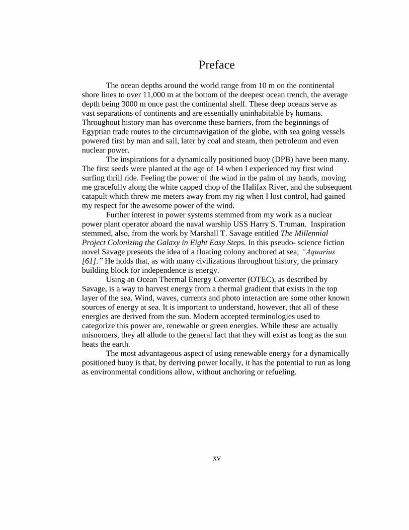
The inspirations for a dynamically positioned buoy (DPB) have been many.
The first seeds were planted at the age of 14 when I experienced my first wind
surfing thrill ride. Feeling the power of the wind in the palm of my hands, moving
me gracefully along the white capped chop of the Halifax River, and the subsequent
catapult which threw me meters away from my rig when I lost control, had gained
my respect for the awesome power of the wind.
Further interest in power systems stemmed from my work as a nuclear
power plant operator aboard the naval warship USS Harry S. Truman. Inspiration
stemmed, also, from the work by Marshall T. Savage entitled The Millennial
Project Colonizing the Galaxy in Eight Easy Steps. In this pseudo- science fiction
novel Savage presents the idea of a floating colony anchored at sea; “Aquarius
[61].” He holds that, as with many civilizations throughout history, the primary
building block for independence is energy.
Using an Ocean Thermal Energy Converter (OTEC), as described by
Savage, is a way to harvest energy from a thermal gradient that exists in the top
layer of the sea. Wind, waves, currents and photo interaction are some other known
sources of energy at sea. It is important to understand, however, that all of these
energies are derived from the sun. Modern accepted terminologies used to
categorize this power are, renewable or green energies. While these are actually
misnomers, they all allude to the general fact that they will exist as long as the sun
heats the earth.
The most advantageous aspect of using renewable energy for a dynamically
positioned buoy is that, by deriving power locally, it has the potential to run as long
as environmental conditions allow, without anchoring or refueling.

xvi
Acknowledgements
Anthony Jones
Abe Stephens
Bill Battin
Thoy Pagliari
John Rodgers
Dr. Stephen Wood
Dr. Robert Sullivan
Dr. Eric Thosteson
Emil Pagliari
Luke Pratte
John Dixson
Bill Bailey
Greg Peebles
Amanda Klein
Edward W. and Lee Hill Snowdon Administrative Fund
1
1. Introduction
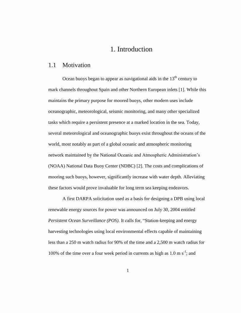
1.1 Motivation
Ocean buoys began to appear as navigational aids in the 13th
century to
mark channels throughout Spain and other Northern European inlets [1]. While this
maintains the primary purpose for moored buoys, other modern uses include
oceanographic, meteorological, seismic monitoring, and many other specialized
tasks which require a persistent presence at a marked location in the sea. Today,
several meteorological and oceanographic buoys exist throughout the oceans of the
world, most notably as part of a global oceanic and atmospheric monitoring
network maintained by the National Oceanic and Atmospheric Administration’s
(NOAA) National Data Buoy Center (NDBC) [2]. The costs and complications of
mooring such buoys, however, significantly increase with water depth. Alleviating
these factors would prove invaluable for long term sea keeping endeavors.
A first DARPA solicitation used as a basis for designing a DPB using local
renewable energy sources for power was announced on July 30, 2004 entitled
Persistent Ocean Surveillance (POS). It calls for, “Station-keeping and energy
harvesting technologies using local environmental effects capable of maintaining
less than a 250 m watch radius for 90% of the time and a 2,500 m watch radius for
100% of the time over a four week period in currents as high as 1.0 m s-1
; and
2
prototype (tactical sized) ocean sensing buoy with continuous RF communications
[3].” A second was announced on July 31, 2008 entitled STATION KEEPING
BUOY ENERGY HARVESTING/HARNESSING. It further identified, “Two primary
challenges for small station keeping buoys (SKBs) that require novel technologies
and concepts [4].” They are, “Maintaining a positive energy balance and operating
for long periods of time on the open ocean [4].” While these grants have already
been awarded, the solicitations do present a likely beginning point for further
development.
A buoy that can maintain a fixed position without a mooring system offers
advantages of remote instrumentation in the deep oceans, where buoy tenders
spend long voyages to maintain. The applications are numerous including remote
instrumentation and sensing, ocean aids to navigation, remote emergency beacons,
telecommunication relay stations, or even a non-space based maritime positioning
system. With readily available computer technology it is feasible to build and
operate such a buoy on a low level budget and at a relatively high level of
precision.
1.2 A Dynamically Positioned Buoy
Using real-time wind and solar energy the DPB can collect, convert, and
redistribute power to two thrusters mounted below the waterline and to six, 12 volt
55 amp-hour absorbed glass mat (AGM) deep cycle batteries for energy storage.
3
The control system uses a Microchip developed PIC18f27J13 onboard
microcontroller to process GPS and magnetometer data from a LOCOSYS
LS20126 module. This chip also controls the set of two trolling motors, used for
buoy positioning via differential drive. The LS20126 also provides 3-axis
accelerometer, real time position, speed and heading data that could be used for
dead reckoning input to an inertial navigation system. This type of system was not
developed for the DPB. Instead, raw accelerometer data is wirelessly transmitted
via a Roving Networks RN-XV, 802.11b/g standard, device with a tested range of
up to 305 m. All raw data from the LS20126 module broadcasted through the RN-
XV chip was received and viewed in two ways. First, using LOCOSYS developed
software GPSFox Utility via virtual serial port emulator [44] [43]. A second
software package was developed for real time data viewing and wireless remote
control of DPB using an Android smart phone. See Appendix A for software
package screenshots. Due to time and cost constraints the renewable energy system
and components are presented as a theoretical design based on electrical load
characteristics found during field tests of the DPB apparatus.
By integrating solar and wind renewable energy systems the feasibility of a
direct motor-generator interaction and energy storage combination, to counteract
the drift effects of current, wind and waves, is considered. This would allow a buoy
to remain in a fixed location at sea without the use of a mooring system.

4
2. Background
2.1 Buoy Designs
A system of moored buoys throughout the worlds’ inland and coastal
waterways, known as the Marine Aids to Navigation (ATON) system, exists today
[9]. These buoy designs vary slightly among different countries and applications,
but, with the exception of a few outliers like special purpose discus and scow types,
ATON buoys are generally one of three design types. The steel can or conical buoy,
the unlighted or lighted beacon buoy, and the spar or ice type buoy are each
designed to be advantageous in different environments. Can and conical buoys
simply float on the ocean surface and are moored to the ocean floor using heavy
chain and rope. Unlighted and lighted offshore buoys are the most common within
the ATON system. The top beacon light is usually raised up by a support structure
that rests on a large floating can buoy ranging from 2.5 – 3.0 m in diameter. Some
of these are also affixed with sound capability, limited to a 400 m range, and Radio
and Beacon (RACON) systems to signal their presence to nearby vessels. The large
surface area and low center of gravity keeps them upright. A spar buoy is
distinguished by a hollow, long and slender, cylindrical body that extends primarily
below the water line. This low cross section and large mass design effectively
reduces the overall influence that surface waves have on the spar buoy. “The

5
Finnish have made extensive use of spar buoys with taut mooring in ice
environments. These buoys have the added benefit of providing a negligible watch
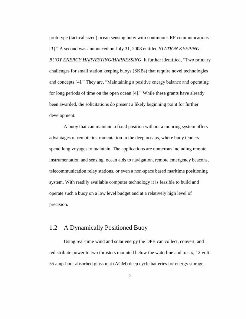
circle since they are essentially a variation of the articulated beacon [9].” Figure 1
shows lighted, spar, and can type buoys.
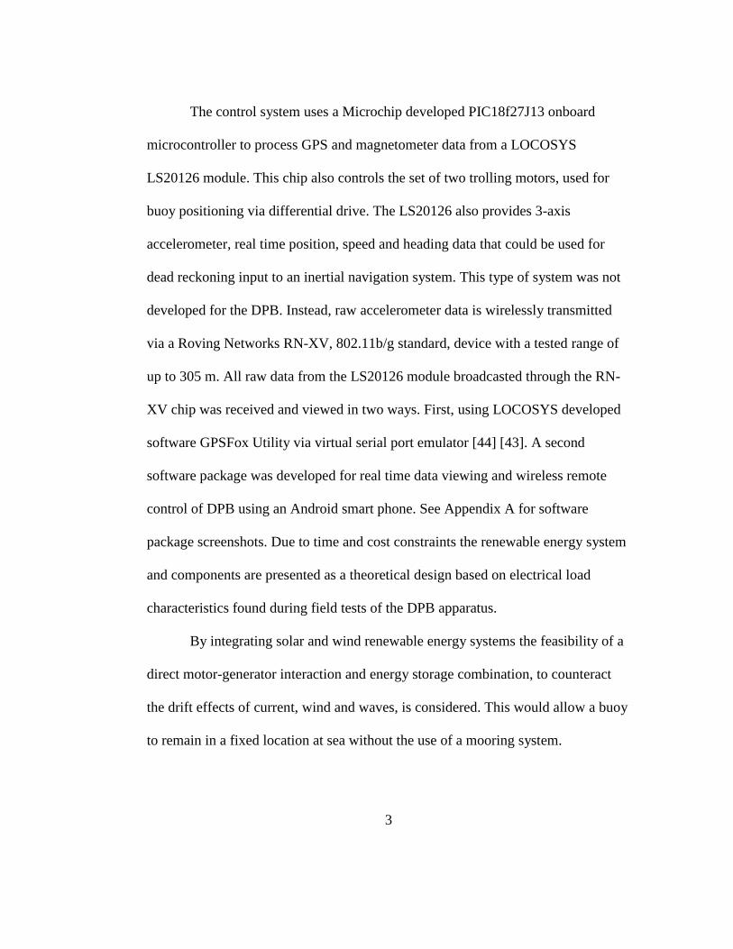
Other buoy designs exist for scientific purposes. Drift buoys and underwater
acoustic buoys are some of these. NOAA’s National Data Buoy Center (NDBC)
deploys and maintains scientific instrumentation buoys throughout the world.
These continually monitor and record meteorological and oceanographic in-situ
data in real time. The data is freely accessible through their website
www.ndbc.noaa.gov [2]. Figure 2 shows NDBC’s collection of scientific buoys.
6
Figure 1 from [9] a) lighted buoy b) spar buoy c) can buoy
7
Figure 2 from [2] NDBC Moored Buoy Program offshore meteorological and
oceanographic buoy collection
8
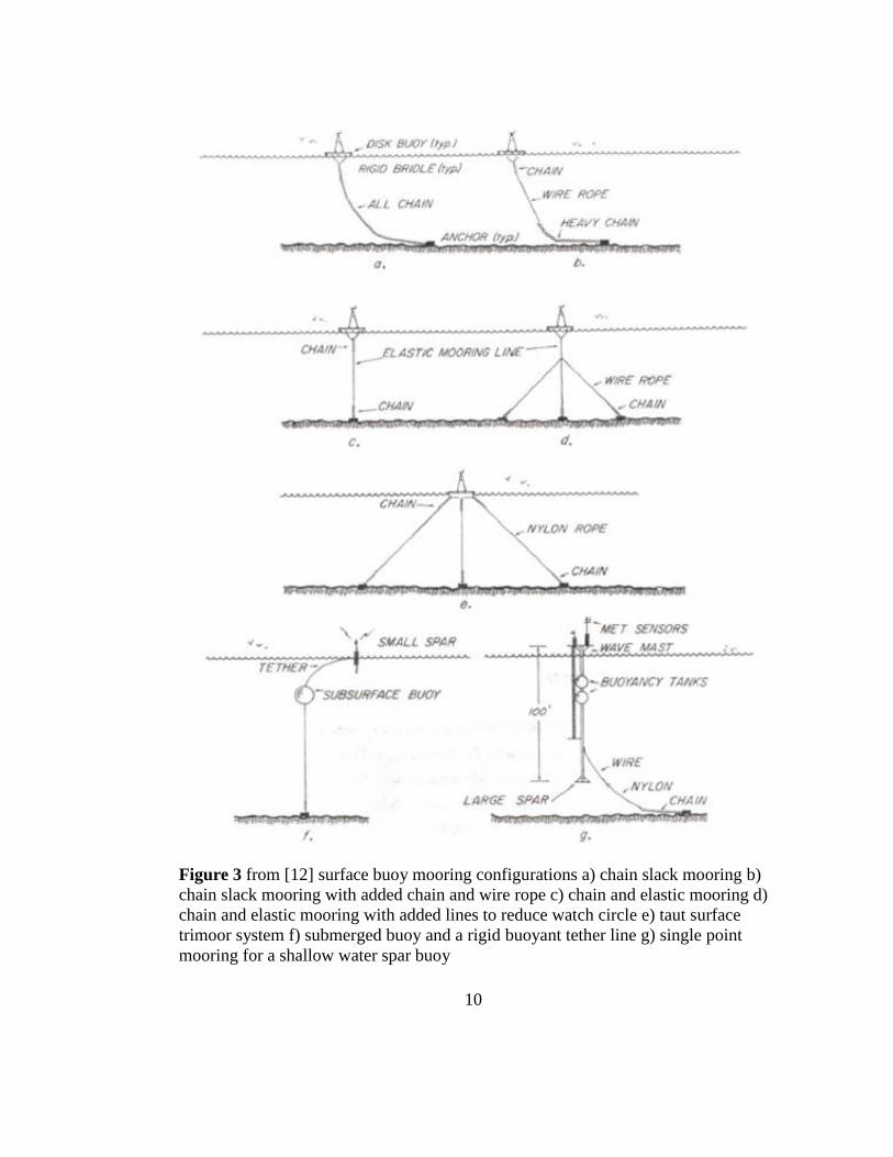
2.1.1 Buoy Moorings
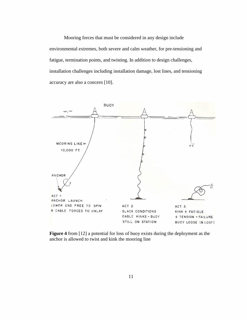
Deep water moored ocean buoys exist in waters as deep as 5800 m in the
Pacific Ocean. Drawbacks to consider when anchoring this deep are the added
weight, material, expense, potential breaks in the mooring line like in Figure 4,
shark bites, etc. Other environmental considerations like damage to sea floor
environments and corals must also be taken into account.
Buoys that traditionally mark a fixed position in the ocean, for navigation or
scientific purposes, are moored to the sea floor with train wheels or iron sinker
weights and tethered with a rope and chain. Deployment may require large rolls of
mooring lines. Some deeper ocean buoys rely on “A combination of chain, nylon,
and buoyant polypropylene materials designed for many years of service [2].”
Typical buoy mooring systems are shown in Figure 3. One common occurrence
among moored buoys is extensive damage from collision with ships. Another is
marine growth. Yet another issue with moored buoys is the maintenance involved.
They require a dedicated buoy tender that is designed to handle the weight of steel
buoys and mooring chains. Some successful experimentation with light weight
glass or fiber reinforced plastics has been done, but most fail after a short time and
are, therefore, not cost effective [9]. Also, depending on the mooring
configuration and buoy design, a large watch circle is required. Because of tide
changes and catenary requirements this radius, which the chain provides the buoy
to roam, reduces the accuracy of marking buoys. While much of the expense

9
involved with deep water mooring systems is from the materials themselves, a large
expense is from the data collection and environmental analysis required before a
mooring is even established offshore. These include parameters such as 100 year
wind and squall statistics, and wave pattern history. Buoy and mooring systems
must be designed to withstand loads in the most extreme conditions. “Modern
mooring designs typically utilize groups of mooring lines to provide redundancy in
the event of a line failure. Spread moored systems typically have mooring lines in
groups at each of the four quadrants of the [Floating Production Storage and
Offloading] FPSO while turret moored vessels utilize three groups of mooring legs
[10].”
10
Figure 3 from [12] surface buoy mooring configurations a) chain slack mooring b)
chain slack mooring with added chain and wire rope c) chain and elastic mooring d)
chain and elastic mooring with added lines to reduce watch circle e) taut surface
trimoor system f) submerged buoy and a rigid buoyant tether line g) single point
mooring for a shallow water spar buoy
11
Mooring forces that must be considered in any design include
environmental extremes, both severe and calm weather, for pre-tensioning and
fatigue, termination points, and twisting. In addition to design challenges,
installation challenges including installation damage, lost lines, and tensioning
accuracy are also a concern [10].
Figure 4 from [12] a potential for loss of buoy exists during the deployment as the
anchor is allowed to twist and kink the mooring line
12
2.2 Oil Rigs
The oil and gas industry has driven much of the deep ocean mooring
technology with the use of semi-submersible and spar type ocean platforms, which
provide stability for offshore drilling. Large pontoons are flooded and submerged
to a predetermined depth, while hollow cylindrical stanchions raise the platform
above the surface waves. This design provides for a minimal cross-section exposed
to the surface currents and gravity waves thereby reducing their influence on the
rig. They also use tension leg moorings to help minimize the sway, surge, and
heave of the platform.
2.3 Dynamic Positioning
As opposed to anchoring, DP is an alternate method of station keeping at
sea. By definition of the International Marine Contractors Association (IMCA),
dynamic positioning is, “The use of systems which automatically control a vessel's
position and heading exclusively by means of active thrust to remain at a fixed
location, for precision maneuvering, tracking and for other specialist positioning
abilities [15].”
Driven mostly by the needs of the oil and gas exploration industry in the
early 1960s, an analogue form of DP was pioneered by Howard Shatto aboard the
vessel “Eureka” in 1961 [15]. Modern forms of DP have propagated across several

13
seafaring industries from passenger cruise lines, for added stability and comfort, to
oceanographic research platforms. Commercial systems use a combination of
differential GPS, real time kinematics or inertial navigation systems, local
environmental sensing, and multi-directional thrusters to consistently locate vessels
within 1 m of accuracy.
Advantages include the elimination of costly anchor handling systems and
materials involved in deep sea operations as well as the preservation of seabed
environmental systems like coral reefs or manmade systems such as pipelines and
ship wrecks. DPS can achieve high levels of positional accuracy at sea, whereas
anchored vessels must maintain a watch radius to accommodate tethering systems.
Regardless of the type of vessel, the three key components of any DP system are
the reference, control, and propulsion systems.
The reference system comprises any components or sensors that provide
information for DP such as position, heading, environmental conditions, etc.
Positioning reference systems determine where the vessel is in reference to where it
is supposed to be in the world, usually by employing advanced GPS, which is
discussed in the following section. The geospatial reference is fed to the control
system along with other common reference information such as vessel heading,
wind speed, and vessel motion or acceleration. User input is another required value
used to establish the desired set points for any automated system.
14
Automated computer systems are the primary means of control for any
modern DPS. Control algorithms include anything from advanced computer
modeling and filtering techniques to proportional integral differential (PID) control
or neural networks. As references and set points are fed into the control system,
control signals are generated and sent to the propulsion and steering systems to
maneuver the vessel into the desired position and keep it there in opposition of
environmental forces.
Power and propulsion systems on ships are comprised of main engines,
rudders, and bow and azimuth thrusters, while on stationary platforms several
directional thrusters are used to correct position differences. Power is usually
provided by diesel-electric generators. Depending on the characteristics of the
vessel and environmental conditions, power requirements for DP tend to be quite
substantial and costly. This, along with the added manpower requirements of
operating and maintain a DP system, makes up the two most restrictive
disadvantages of DP over other methods of station keeping at sea. Both of which
could be overcome, by using integrated renewable energy systems and a fully
automated control system.
2.4 Navigation, GPS, and DGPS
The task of navigating and locating something on the earth’s surface has
been a part of life ever since humans roamed the earth throughout history. Using
15
landmarks was a known and obvious way to do this, but when it came to wide open
spaces like the ocean, navigators were only equipped with instincts and other crude
processes such as dead reckoning. Dead reckoning is a technique of periodically
plotting distance and direction traveled on a nautical chart to keep track of location.
“A better method arose around 1100 CE, when the Chinese created the first
magnetized needle compass [16].” Until the invention of the sextant in the 1731,
sailors who ventured out of sight of landmarks could only estimate latitudes based
on key celestial markers like the sun or the North Star. They also relied on natural
indicators such as currents and bird migratory patterns. Tracking longitudinal
positions was never possible until the mid-1700s when John Harrison invented the
first precision chronometer. Three key contributions that further advanced the
accuracy of modern global positioning were the global adoption of Greenwich
Mean Time (GMT) in the late 1800s, the propagation of aviation, and the invention
of radar in the early 1900s [16].
Using radio beacon signals at known locations, airplanes and boats no
longer needed to rely on celestial bodies which were traditionally useless in adverse
cloud conditions. In the 1960s a well-known network of radio beacon towers was
known as Location Radio Aids to Navigation (LORAN). This system became
obsolete with the introduction of GPS and was discontinued in the US in 2010.
The well-known satellite Global Positioning System (GPS) of today was
originally developed by the US Department of Defense. This constellation of 24,
16
geosynchronous, satellites was commissioned and launched in 1978 by the USAF
[17]. To determine any location on earth, the process of trilateration uses distance
measurements between the positioned object and at least four different satellites in
orbit. Using radio waves, pseudo random code, and atomic clocks for timing
accuracy, a GPS receiver can locate itself anywhere on earth within 10 m accuracy.
The reason for this limitation is because unpredictable disruptions of the signals
occur within the earth’s atmosphere which distorts the distance measurements.
To overcome this, Differential GPS (DGPS) ground stations, in the vicinity
of the roving GPS receiver, calculate the timing errors in the atmosphere and
transmit this correction factor to GPS units via radio transmissions. More recently,
using wide area networks (WAN) has allowed multiple reference stations to
collaborate data providing an even better timing correction for more accurate
positioning.
2.5 Renewable Energy
To examine the feasibility of renewable energy as a source for the DPB
project it is important to understand the potential sources and what they can
provide. When dealing with electricity, units of energy are measured in watt hours
(Wh) and power in watts (W).
17
2.5.1 Wind Power
“The earliest mention of windmills in actual use is from India about 2400
years ago [11].” The first ones used to generate electricity, wind turbines, were
designed in the late 1800s [8]. Generally, wind is developed by temperature
gradients in the earth’s atmosphere. Effects from surface topography, temperature
effects on density, rotation of the earth, time of day, time of year, and location on
earth are some of the causes of variability and diminished wind speeds. The amount
of energy in a strong wind is primarily derived from the speed and the mass of the
moving air. The primary advantage of using wind power in offshore environments
is that unobstructed airflow over large areas allows wind speed to accumulate. Air
density is also fairly constant and highest, 1.225 kg/m3
at 15°C, at sea level [8].
Wind turbines convert linear air motion to rotational kinetic energy. The
spinning shaft of the turbine is coupled to a generator to produce electric power. All
wind turbines have essentially three main components, a tower, a nacelle, and the
rotors.
The tower is simply the mast on top of which the turbine assembly is
mounted. The nacelle is the body which houses the sensitive components of the
wind machine such as the electric generator, gearing, slip rings, etc. to protect them
from environmental elements.
The rotors are arguably the most important part of a wind turbine. They are
the mechanisms coupled to the electric generator’s shaft which react to the linear
18
air motion causing it to rotate. The entire power capacity of a wind turbine can be
traced back to the rotors. The characteristics of the rotor blades are so instrumental
in determining the usefulness of the wind turbine that Gipe makes the general
classification of wind turbines based on the diameter of their rotor blades. Small
includes anything under 10 m in diameter, medium, 10 m to 60 m, and large or
giant-sized for anything over that.
When dealing with wind turbines “A” in equations 2.1, 2.2, and 2.3 refers to
the swept area of the rotor blades and is calculated using the geometric formula for
the area of a circle.
Where radius, r, is half of the rotor diameter.
The general formula for wind energy is given by
Where V is velocity and mass is broken down into area and density, ρ. Because the
air is moving, the time component, t, must also be included for completeness. Wind
power being an instantaneous measure, the time component is divided out giving
Power is simply measured in Watts (W). Equation 2.3 shows that the cubed
velocity, or wind speed, component has the most influence on the total amount
available power in a wind stream.
19
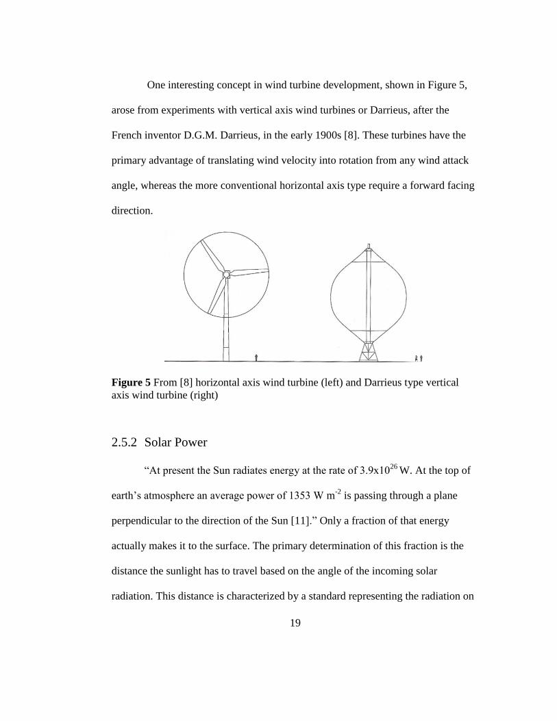
One interesting concept in wind turbine development, shown in Figure 5,
arose from experiments with vertical axis wind turbines or Darrieus, after the
French inventor D.G.M. Darrieus, in the early 1900s [8]. These turbines have the
primary advantage of translating wind velocity into rotation from any wind attack
angle, whereas the more conventional horizontal axis type require a forward facing
direction.
Figure 5 From [8] horizontal axis wind turbine (left) and Darrieus type vertical
axis wind turbine (right)
2.5.2 Solar Power
“At present the Sun radiates energy at the rate of 3.9x1026
W. At the top of
earth’s atmosphere an average power of 1353 W m-2
is passing through a plane
perpendicular to the direction of the Sun [11].” Only a fraction of that energy
actually makes it to the surface. The primary determination of this fraction is the
distance the sunlight has to travel based on the angle of the incoming solar
radiation. This distance is characterized by a standard representing the radiation on

20
earth’s surface known as the air mass coefficient. The highest amount of solar
irradiance is achieved when the sun is directly overhead near the equator,
correlating to a zenith angle of 0° and one standard air mass (AM1). The standard
used to measure solar energy system performance is set forth by the American
Society for Testing and Materials (ASTM). “ASTM G173 - 03(2008) Standard
Tables for Reference Solar Spectral Irradiances: Direct Normal and Hemispherical
on 37° Tilted Surface” sets this standard to AM1.5, which correlates to a zenith
angle of 48.19° and an irradiance of 1000 W m-2
[64]. Other factors which affect
solar insolation include environmental conditions such as cloud cover, rain, etc.
Some systems convert this energy to electric power using direct heat, usually by
concentrating the radiation on one central area with mirrors, and some form of heat
engine such as a steam turbine or sterling engine. Another, more common, way is
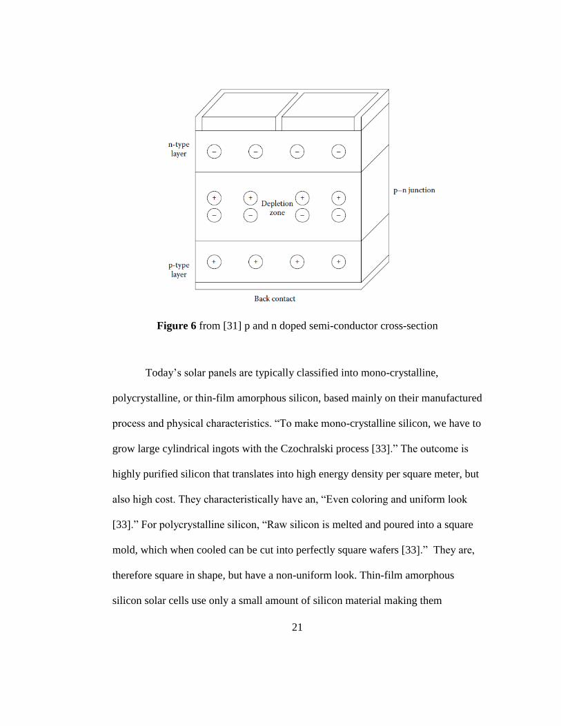
by using solar cells. Solar cells convert the power contained within the radiation to
DC voltage using a combination of specially p and n doped semi-conductive
materials, photo-interactions, and conductive metal contacts as depicted in Figure 6
[31].
21
Figure 6 from [31] p and n doped semi-conductor cross-section
Today’s solar panels are typically classified into mono-crystalline,
polycrystalline, or thin-film amorphous silicon, based mainly on their manufactured
process and physical characteristics. “To make mono-crystalline silicon, we have to
grow large cylindrical ingots with the Czochralski process [33].” The outcome is
highly purified silicon that translates into high energy density per square meter, but
also high cost. They characteristically have an, “Even coloring and uniform look
[33].” For polycrystalline silicon, “Raw silicon is melted and poured into a square
mold, which when cooled can be cut into perfectly square wafers [33].” They are,
therefore square in shape, but have a non-uniform look. Thin-film amorphous
silicon solar cells use only a small amount of silicon material making them
22
significantly cheaper and easier to manufacture. “Depending on the technology,
thin-film module prototypes have reached efficiencies between 7–13% and
production modules operate at about 9% [33].”
Power rating of solar panels is a balance between overall efficiency and
density, the main difference being the amount of area the panels require to produce
their nominal output. As of December 12, 2011, according to [32], the most
efficient modules commercially available, based on power density, are between
15.24% - 16.00% using polycrystalline silicon modules.
2.5.3 Energy Storage
“In 1859, the French physicist Gaston Planté invented the first rechargeable
battery. It was based on lead acid, a system that is still used today [41].” Variations
of the lead acid battery are typically used with hybrid energy systems as a means of
consistently meeting load requirements. The benefits of lead acid, versus other
popular battery chemistries such as nickel-metal-hydride and lithium-ion, are the
comparatively low cost of manufacturing, simplicity of charging, wide range of
operating temperatures, and consistent, reliable discharge characteristics.
Another consideration for a battery storage system aboard DPB is the wide
range of rolling and pitching motions associated with offshore environments. In
flooded lead acid battery, the electrolyte solution is allowed to slosh around causing
spillage and harmful gas build up. They also require a small amount of
23
maintenance which is undesirable for DPB. An alternative is the use of sealed lead
acid batteries, which use either an impregnated gel or an absorbed glass mat
(AGM) electrolyte in a completely sealed container. They require no maintenance
and are not susceptible to spillage [41].
A third, important consideration for hybrid energy system battery storage is
the amount of cycling it will undergo. When it comes to lead acid batteries there are
two different types, starter and deep cycle. The starter battery is designed to
provide high output for short periods of time while the deep cycle battery can
handle longer and deeper discharges due to thicker lead plating. For DPB a deep
cycle type AGM battery is preferred [41].
2.6 Similar Systems
A few U.S. patents, having similar motives to DPB, have been awarded.
SKB using SONAR reflector or active transponder anchored to the sea floor: US
Patent 3,369,516 was awarded to inventor Roger J. Pierce on February 20, 1968
entitled, “STABLE OCEANIC STATION”. The propulsion proposed is a,
“Tangential jet [23]” using atomic power. SKB using GPS: US Patent 5,577,942
was awarded to inventor Gregory J. Juselis on November 26, 1996 entitled,
“STATION KEEPING BUOY SYSTEM”. The propulsion proposed is a, “Bi-
directional vector thrust system [21]” using batteries. A self-orientating water drift
compensation method using passive hydrofoil device: US Patent 2009/0095208 A1

24
was awarded to Cardoza et al. on April 16, 2009 entitled, “WATER DRIFT
COMPENSATION METHOD AND DEVICE [22]” also using batteries.
Unmanned ocean vehicle using winged sail covered with photovoltaic cells: US
Patent 7,789,723 was awarded to Dane et al. on September 7, 2010 entitled,
“UNMANNED OCEAN VEHICLE [24]” using hybrid wind and solar power.
There are several maritime vehicles out there that are not buoys. The main
distinctions of DPB are a combination of the intended purpose and the hybrid
power system. DPB is not an autonomous surface vehicle designed to transit long
distances in the ocean. Instead, it is intended to be optimized for station keeping,
with an emphasis on the use of renewable energy systems to help maintain position.
Some general applications for DPB could include remote location aids to
navigation, surveillance, and sea-air interface communication systems. The
following section examines some recent developments in both ASV’s and mobile
buoys.
The most similar systems to DPB were developed, and at least partially
funded, in response to the [3] and [4] calling for sea power and surveillance.
SeaLandAire Technologies, Inc. owns two projects, Persistent Ocean Surveillance
– Station Keeping Buoy (POS-SKB) and Gatekeeper, which have successfully
demonstrated the abilities of station keeping and energy harvesting.
“SeaLandAire’s hardware successfully maintained station in adverse marine
environments for over 120 hours, averaging less than 3 meters deviation from the
25
designated station keeping point [26].” Another SKB system with the same name,
Gatekeeper, was developed by Falmouth Scientific Inc. in 2008. This system uses a
proprietary Salt Water Activated Power System (SWAPS) by Mil3, Inc. to generate
200 watts using a combination of reactive metal and hydrogen fuel cells [27]. A
third noteworthy system was developed by the Johns Hopkins University Applied
Physics Laboratory in 2006. It uses a combination of sail and auxiliary thruster for
positioning. “The SKB was successful in station keeping within the 250-m watch
radius 90% of the time and within a 1000-m watch radius 100% of the time [25].”
Spar buoy designs provide another kind of station keeping advantage, but
are a hydro dynamical disadvantaged when transiting. A scaled spar platform with
dynamic positioning capability was considered in [14]. Although unrelated to
renewable energy systems, this adapted Floating Instrument Platform (FLIP)
demonstrates a scaled dynamic positioning system requiring 12 thrusters for six
degrees of motion to position and stabilize a spar buoy platform.
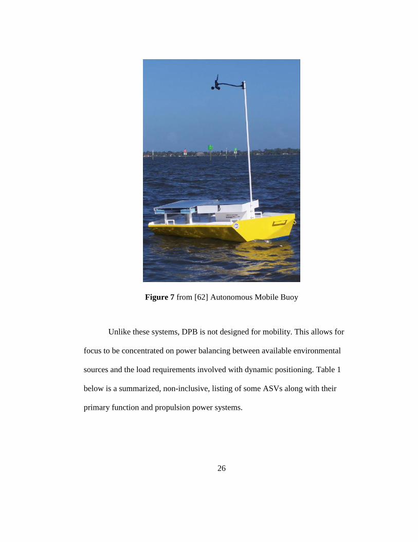
One other noteworthy system, developed outside the realm of DARPA or
SBIR funding, is Florida Institute of Technology’s Autonomous Mobile Buoy, a
thesis by Adam S. Outlaw in 2007 and shown in Figure 7. It was designed for
waypoint tracking and station keeping using an automated anchor and 30 m tether,
limiting its effectiveness to littoral seas. A renewable energy element was added
using solar panels to recharge the system while anchored [13] [62].
26
Figure 7 from [62] Autonomous Mobile Buoy
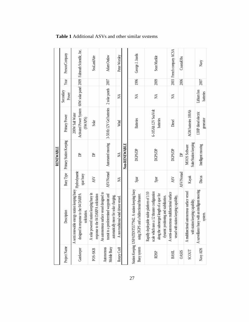
Unlike these systems, DPB is not designed for mobility. This allows for
focus to be concentrated on power balancing between available environmental
sources and the load requirements involved with dynamic positioning. Table 1
below is a summarized, non-inclusive, listing of some ASVs along with their
primary function and propulsion power systems.
27
Proj
ect N
ame
Des
crip
tion
Buoy
Typ
ePr
imar
y St
atio
n K
eepi
ngPr
imar
y Po
wer
Seco
ndar
y
Pow
erY
ear
Pers
on/C
ompa
ny
Gat
ekee
per
A se
mi r
enew
able
ener
gy st
atio
n ke
eping
buo
y
desig
ned
in re
spon
se to
the
04 D
ARP
A
solic
itatio
n.
Hyd
rody
nam
ic
spar
buo
yD
P
200W
Salt
Wat
er
Act
ivate
d Po
wer
Sys
tem
(SW
APS
)
60W
solar
pan
el20
09Fa
lmou
th S
cient
ific, I
nc.
POS-
SKB
A so
lar p
ower
ed st
atio
n ke
eping
buo
y in
resp
onse
to th
e 04
DA
RPA
solic
itatio
nA
SVD
PSo
larSe
aLan
dAire
Aut
onom
ous
Mob
ile B
uoy
An
auto
nom
ous s
urfa
ce v
esse
l des
igned
to
trans
it to
a p
rede
term
ined
way
point
and
auto
mat
ically
moo
r for
solar
cha
rging
.
ASV
/Nom
adA
utom
ated
moo
ring
3-50
Ah
12V
Gel
batte
ries
2 so
lar p
anels
2007
Ada
m O
utlaw
Rota
ry C
raft
A n
on tr
aditio
nal w
ind d
riven
ves
sel.
NA
NA
Wind
NA
Pete
r Wor
sley
Stat
ion
Kee
ping
Buoy
syste
m
USP
ATE
NT5
5779
42. A
stat
ion
keep
ing b
uoy
using
DG
PS a
nd a
bid
irect
iona
l thr
uste
r.Sp
ar
DG
PS/D
PBa
tterie
sN
A19
96G
eorg
e J.
Juse
lis
RDSP
Rapi
dly
depl
oyab
le sta
ble
plat
form
of 1
/10
scale
whic
h us
es a
12
thru
ster c
onfig
urat
ion
along
the
subm
erge
d len
gth
of a
spar
for
dyna
mic
posit
ionin
g an
d sta
biliz
atio
n.
Spar
D
GPS
/DP
6-10
5Ah
12V
Sea
Vol
t
batte
ries
NA
2009
Sean
Mar
ikle
BASI
LA
sem
i-aut
onom
ous m
ultifu
nctio
nal s
urfa
ce
vess
el w
ith st
atio
n ke
eping
cap
abilit
y,A
SVD
GPS
/DP
Dies
elN
A20
03Fr
ench
com
pany
AC
SA
OA
SIS
ASV
/Nom
adD
P20
06C
oasta
lObs
SCO
UT
A m
ultifu
nctio
nal a
uton
omou
s sur
face
ves
sel
with
stat
ion
keep
ing c
apab
ility.
Kay
akM
OO
S So
ftwar
e
Suite
/Sta
tion
keep
ingA
GM
bat
terie
s 100
Ah
Nav
y A
DS
A su
rveil
lance
buo
y w
ith a
n int
ellige
nt m
oorin
g
syste
m.
Disc
usIn
tellig
ent m
oorin
g13
HP
dies
el ele
ctric
gene
rato
r
Lith
ium Io
n
batte
ries
2007
Nav
y
Non
-RE
NE
WA
BL
E
RE
NE
WA
BL
E
Table 1 Additional ASVs and other similar systems
similar systems
28
3. Development and Construction
3.1 Design Considerations
The DPB concept for this project was derived from a previously proposed
rotary electric wind craft “Windmill Ship” design and analysis. As work progressed
on the original project it was determined too broad of scope and focus was shifted
to low cost dynamic positioning and integrated power systems. For theoretical
design purposes of a DPB, however, it is helpful to examine a well proven physical
paradigm presented by Professor B.L. Blackford of Dalhousie University in [18].
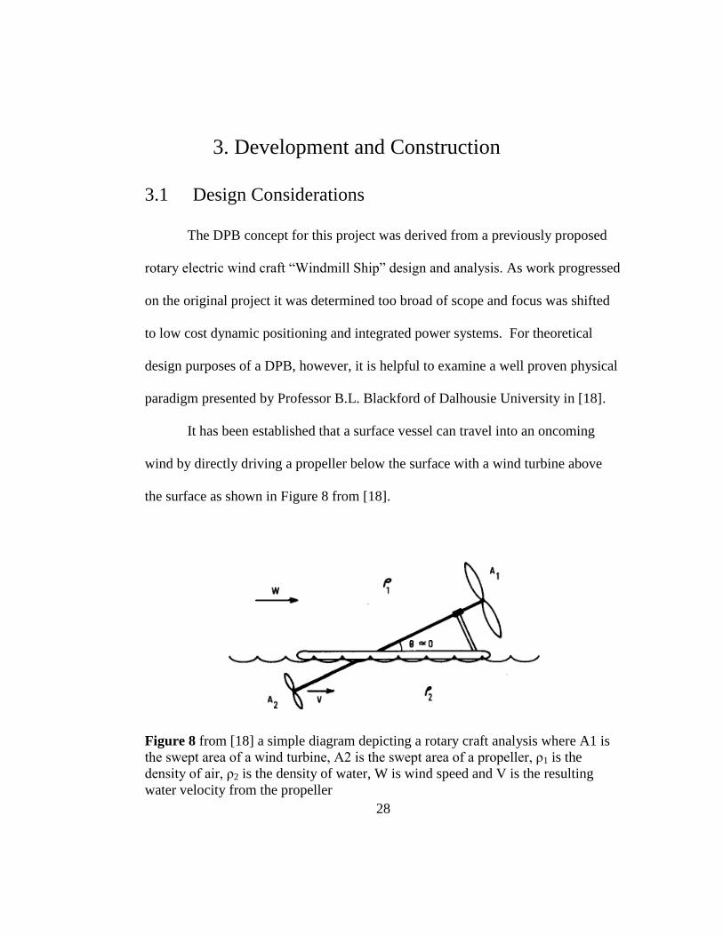
It has been established that a surface vessel can travel into an oncoming
wind by directly driving a propeller below the surface with a wind turbine above
the surface as shown in Figure 8 from [18].
Figure 8 from [18] a simple diagram depicting a rotary craft analysis where A1 is
the swept area of a wind turbine, A2 is the swept area of a propeller, ρ1 is the
density of air, ρ2 is the density of water, W is wind speed and V is the resulting
water velocity from the propeller
29
The key principles that allow for this are both the ratios between the surface area of
the turbine and the propeller, A1/A2, and the differences in density of air and
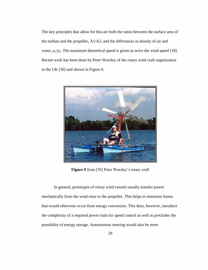
water, ρ1/ρ2. The maximum theoretical speed is given as twice the wind speed [18].
Recent work has been done by Peter Worsley of the rotary wind craft organization
in the UK [30] and shown in Figure 9.
Figure 9 from [30] Peter Worsley’s rotary craft
In general, prototypes of rotary wind vessels usually transfer power
mechanically from the wind rotor to the propeller. This helps to minimize losses
that would otherwise occur from energy conversion. This does, however, introduce
the complexity of a required power train for speed control as well as precludes the
possibility of energy storage. Autonomous steering would also be more

30
burdensome for a mechanical system and would require, at minimum an
electromechanical system in order to interface with the DP control circuit.
An all-electric system does present higher losses involved with energy
conversion, but makes automated energy storage, speed control, and steering quite
manageable with the DPB control system interface.
3.1.1 Pre-existing Buoy Project
The yellow surface buoy was previously conceived and commissioned by
Dr. Stephen Wood, at Florida Institute of Technology, in 2009 and remains readily
available. The initial design intent was to provide a low cost solution for an
offshore moored buoy. Figure 10 a) is a rendering of the initial design from Pro-
Engineer and b) shows the final prototype constructed in 2007.
Using an iterative design process, several configurations were considered to
accommodate a hybrid renewable energy system and thrust capability aboard the
original yellow buoy. These considerations were size restrictions, structural
integrity, buoyancy, and stability.
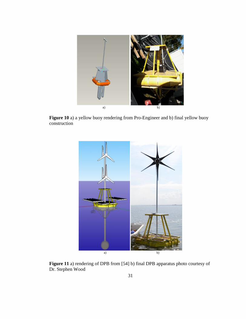
It was suggested by Dr. Stephen Wood that adding an extended length of
pipe below the surface could help to mitigate drift by acting as a type of drag
anchor as well as provide increased stability. Based on these considerations, a final
design rendering, shown in Figure 11 a), was made using [46]. Figure 11 b) shows
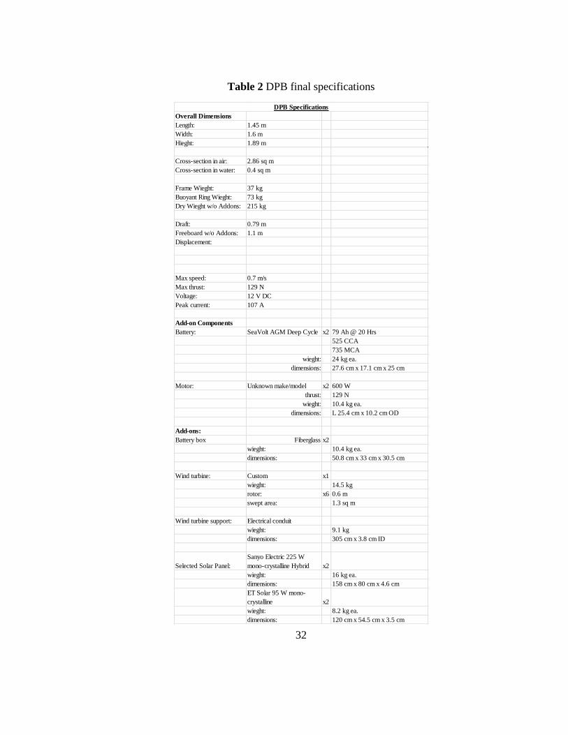
the final construction of DPB and Table 2 is a listing of final DPB specifications.
31
Figure 10 a) a yellow buoy rendering from Pro-Engineer and b) final yellow buoy
construction
Figure 11 a) rendering of DPB from [54] b) final DPB apparatus photo courtesy of
Dr. Stephen Wood
32
Table 2 DPB final specifications
Overall Dimensions
Length: 1.45 m
Width: 1.6 m
Hieght: 1.89 m
Cross-section in air: 2.86 sq m
Cross-section in water: 0.4 sq m
Frame Wieght: 37 kg
Buoyant Ring Wieght: 73 kg
Dry Wieght w/o Addons: 215 kg
Draft: 0.79 m
Freeboard w/o Addons: 1.1 m
Displacement:
Max speed: 0.7 m/s
Max thrust: 129 N
Voltage: 12 V DC
Peak current: 107 A
Add-on Components
Battery: SeaVolt AGM Deep Cycle x2 79 Ah @ 20 Hrs
525 CCA
735 MCA
wieght: 24 kg ea.
dimensions: 27.6 cm x 17.1 cm x 25 cm
Motor: Unknown make/model x2 600 W
thrust: 129 N
wieght: 10.4 kg ea.
dimensions: L 25.4 cm x 10.2 cm OD
Add-ons:
Battery box Fiberglass x2
wieght: 10.4 kg ea.
dimensions: 50.8 cm x 33 cm x 30.5 cm
Wind turbine: Custom x1
wieght: 14.5 kg
rotor: x6 0.6 m
swept area: 1.3 sq m
Wind turbine support: Electrical conduit
wieght: 9.1 kg
dimensions: 305 cm x 3.8 cm ID
Selected Solar Panel:
Sanyo Electric 225 W
mono-crystalline Hybrid x2
wieght: 16 kg ea.
dimensions: 158 cm x 80 cm x 4.6 cm
ET Solar 95 W mono-
crystalline x2
wieght: 8.2 kg ea.
dimensions: 120 cm x 54.5 cm x 3.5 cm
DPB Specifications

33
3.2 DPB Build
The original buoy was not designed for mobile operation and, therefore, had
no corrective capability. Onboard power requirements of the original design were
also limited to minimal instrumentation loads in the 1 to 5 watt range as opposed to
DPB thruster loads in the kilowatt range.
Waterproof battery housings were designed and built for DPB using coarse
fiberglass and West Marine epoxy system in order for DPB to accommodate two
72-Ah deep-cycle AGM batteries. Each housing was wood reinforced with two 2 X
4’s on the bottom forward floor to support the batteries and one 2 X 6 on the aft
bulkhead for the trolling motor addition as shown in Figure 12.
Figure 12 reinforced waterproof battery housing and motor mount
34
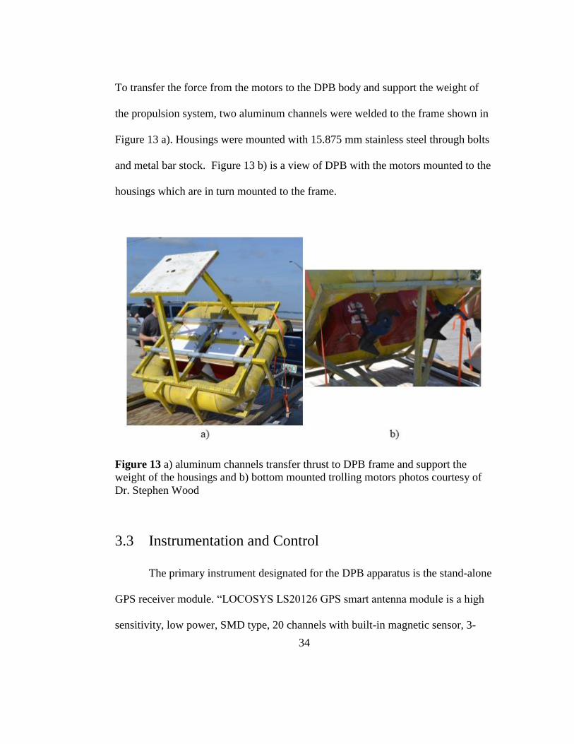
To transfer the force from the motors to the DPB body and support the weight of
the propulsion system, two aluminum channels were welded to the frame shown in
Figure 13 a). Housings were mounted with 15.875 mm stainless steel through bolts
and metal bar stock. Figure 13 b) is a view of DPB with the motors mounted to the
housings which are in turn mounted to the frame.
Figure 13 a) aluminum channels transfer thrust to DPB frame and support the
weight of the housings and b) bottom mounted trolling motors photos courtesy of
Dr. Stephen Wood
3.3 Instrumentation and Control
The primary instrument designated for the DPB apparatus is the stand-alone
GPS receiver module. “LOCOSYS LS20126 GPS smart antenna module is a high
sensitivity, low power, SMD type, 20 channels with built-in magnetic sensor, 3-

35
axis acceleration sensor L1 GPS receiver and 10 mm patch antenna designed for
portable applications [5].” It was selected as a low cost unit with compatible
interfacing to the selected microcontroller via USART, low 3.3 volt CMOS levels,
and a wide range of operating voltage characteristics. It was selected over the
popular LassenTM
iQ GPS receiver module from Trimble which only has a 12-
channel receiver with no built-in magnetic or acceleration sensing. The Trimble
unit also requires an external antenna and connector cable unlike the stand-alone
capability of the LS20126. Both output position solutions at 1Hz in standard
National Marine Electroincs Association (NMEA) format, have similar start-up
times, and similar electrical characteristics. The PIC18F27J13 microcontroller was
selected due to its compatible voltage levels, onboard storage capacity, multiple
interface peripherals, and personal preference.
3.3.1 GPS Receiver Module
The LS20126 module contains a 20-channel GPS receiver with onboard
antenna for latitude and longitude positioning solutions, a magnetometer for
direction and heading, and an accelerometer for attitude sensing and dead
reckoning capability intended for future development. Three-axis attitude data may
also be used for orientation and wave data measurement. Serial output from the
module is communicated at 1Hz on the TX pin following the NMEA developed
standard protocol for maritime electronic systems (NMEA 0183).
36
For GPS, this standard set includes $GPGGA, for Global Positioning
System Fixed Data, $GPGLL Geographic Position – Latitude / Longitude,
$GPGSA, GNSS DOP and Active Satellites, $GPGSV, GNSS Satellites in View,
$GPRMC, Recommended Minimum Specific GNSS Data, and $GPVTG, Course
Over Ground and Ground Speed. Aside from the standard GPS output strings, the
unit output includes proprietary strings which carry the magnetic sensor and
accelerometer data. They are $PLSR,245,1, calibration and acceleration report,
$PLSR,245,2, attitude, and $PLSR,245,7, 3D GPS speed output (ECEF coordinate)
[5]. Table 3 describes the LS20126 minimum recommended output string,
$GPRMC,053740.000,A,2503.6319,N,12136.0099,E,2.69,79.65,100106,,,A*53.
Picking out information for the microcontroller to use is a process called parsing
which will be covered further in the software and application section 3.4.
37
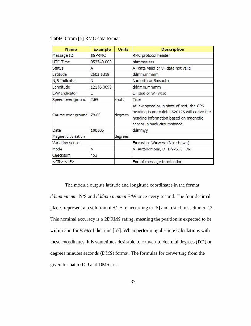
Table 3 from [5] RMC data format
The module outputs latitude and longitude coordinates in the format
ddmm.mmmm N/S and dddmm.mmmm E/W once every second. The four decimal
places represent a resolution of +/- 5 m according to [5] and tested in section 5.2.3.
This nominal accuracy is a 2DRMS rating, meaning the position is expected to be
within 5 m for 95% of the time [65]. When performing discrete calculations with
these coordinates, it is sometimes desirable to convert to decimal degrees (DD) or
degrees minutes seconds (DMS) format. The formulas for converting from the
given format to DD and DMS are:

38
( ⁄ ) (
⁄ )
Where dd is degrees, mm is the integer part of the minutes given by mm.mmmm,
and .mmmm is the remaining fractional part of the given minutes. See Appendix B
for the corresponding “get_position” function showing the implementation of all
coordinate conversions coded in PIC C18.
In practice, because modern day GPS systems use trilateration, a range-
range process requiring precise timing to calculate position, and because radio
signal interactions with the troposphere and ionosphere causes slight variations in
this timing, raw GPS coordinate data tends to be noisy, hence a +/-5 m accuracy.
Another factor when considering a floating platform in the ocean is the
environmental effects of wind, waves and current. Kalman filtering is a method
commonly used to account for all of the system noise involved with DPS. It is an
iterative algorithm, based on Riccati gain equations, system modeling, and process
noise that attempts to calculate an accurate position, or system state. Three basic
steps performed during each iteration of the Kalman filter are, a real-time
measurement is taken, a correction is applied to a previously estimated state
prediction based on that measurement, and a new estimated state is projected
forward to the next iteration.
It is noteworthy that for a typical DPS an extended Kalman filter is usually
implemented to account for the slightly non-linear nature of offshore positioning
39
caused by wind, current, and waves. The DPB designed for this thesis is not
equipped to implement such filtering due to limited program memory, processing
power, and lack of environmental sensors. Instead, DPB uses a 0th order, linear
Kalman filter, based on [19], applied to the LS20126 module output in a simple
attempt to clean up noisy data. See section 5.2.4 for results of an applied filter. See
Appendix B for the corresponding “kalman_filter” function showing the
implementation of the filtering algorithm coded in PIC C18.
A valuable, open source, computer software package developed by Google,
Inc. was developed and released in 2005. Google Earth allows analysis of GPS data
based on the WGS 84 Datum [45]. Some precision and accuracy testing of Google
Earth projections in conjunction with the LS20126 module used on DPB was done
using National Geodetic Society benchmarks and differential GPS systems.
3.3.2 Waypoint Tracking and Positioning
A waypoint generally refers to a set of coordinates referencing a particular
location on the earth. In relation to DPB, this waypoint is considered to be the
marked position where the buoy is deployed. It is intended to be set manually by
the user at the time of deployment, and remain unchanged for the lifetime of that
deployment. To better understand waypoint tracking and positioning it is important
to realize the differences between courses over ground (COG), heading (HDG), and
bearing (BRG). An insightful distinction is given in [20]. “Stand at the Helm and
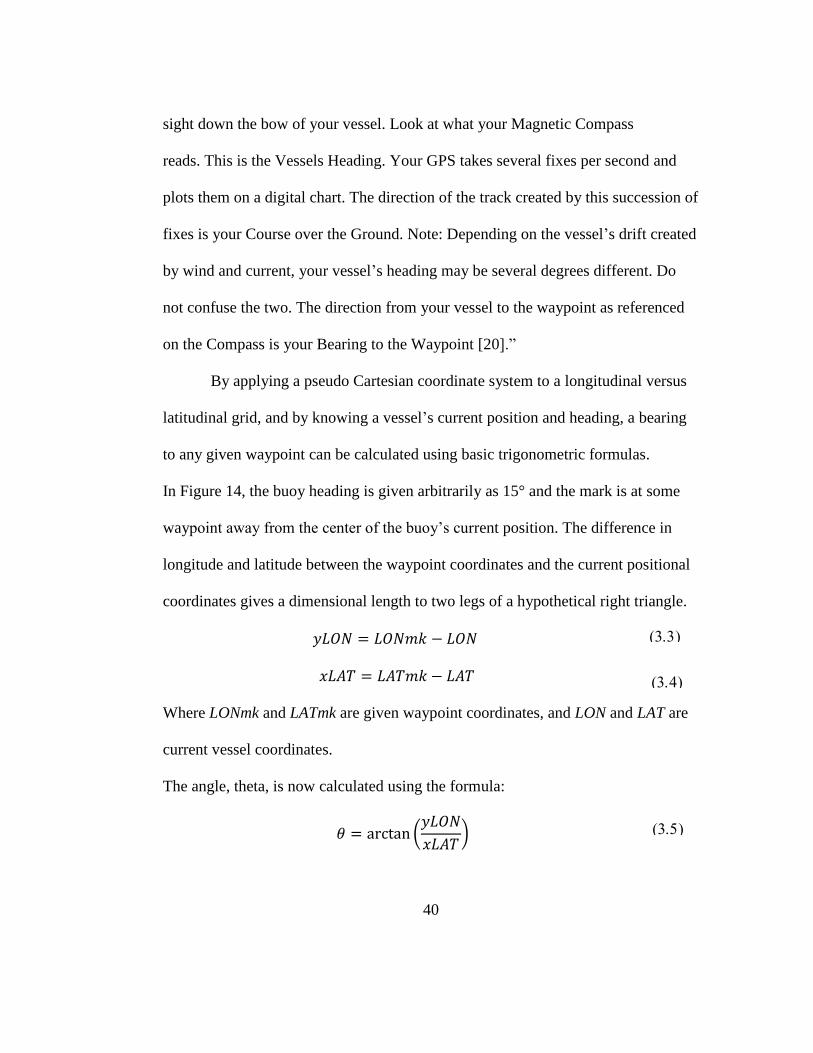
40
sight down the bow of your vessel. Look at what your Magnetic Compass
reads. This is the Vessels Heading. Your GPS takes several fixes per second and
plots them on a digital chart. The direction of the track created by this succession of
fixes is your Course over the Ground. Note: Depending on the vessel’s drift created
by wind and current, your vessel’s heading may be several degrees different. Do
not confuse the two. The direction from your vessel to the waypoint as referenced
on the Compass is your Bearing to the Waypoint [20].”
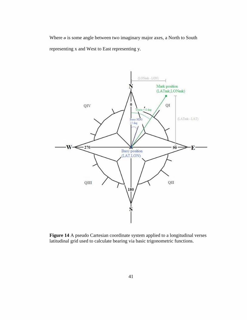
By applying a pseudo Cartesian coordinate system to a longitudinal versus
latitudinal grid, and by knowing a vessel’s current position and heading, a bearing
to any given waypoint can be calculated using basic trigonometric formulas.
In Figure 14, the buoy heading is given arbitrarily as 15° and the mark is at some
waypoint away from the center of the buoy’s current position. The difference in
longitude and latitude between the waypoint coordinates and the current positional
coordinates gives a dimensional length to two legs of a hypothetical right triangle.
Where LONmk and LATmk are given waypoint coordinates, and LON and LAT are
current vessel coordinates.
The angle, theta, is now calculated using the formula:
(
)
41
Where ѳ is some angle between two imaginary major axes, a North to South
representing x and West to East representing y.
Figure 14 A pseudo Cartesian coordinate system applied to a longitudinal verses
latitudinal grid used to calculate bearing via basic trigonometric functions.
42
It is important to note that coordinate positions should be in positive and
negative decimal format so that if the waypoint position is not in the same global
proximity, which might occur at locations on or near the equator and meridians, the
tracking algorithm still holds true in most locations on earth. Special cases arise in
the Pacific Ocean across the 180° meridian and in the Arctic Oceans across the
poles where, for obvious reasons, the simple tracking algorithm breaks down.
While these special cases would be important to incorporate into global tracking
algorithms meant for transects on the order of kilometers, they are not considered
for DPB which is only designed to correct for small offsets in position on the order
of tens of meters.
Again, using the pseudo Cartesian coordinate system, the marked location
must be sorted into one of the four imaginary quadrants based on the values of
yLON and xLAT. This information can then be used to determine the bearing to the
waypoint in relation to the current position by adding ѳ to the axis referencing that
quadrant. For instance, if yLON and xLAT are both negative, the waypoint is in
Quadrant I and the angle theta is exactly the bearing in which the buoy heading
needs to match; therefore the bearing is ѳ + 0°. If the waypoint is in QII, yLON is
negative and xLAT is positive and the bearing becomes ѳ + 90°, and so on. Table 4
provides a full listing of the sorting equations and exceptions that occur when the
waypoint lies directly on an axis.
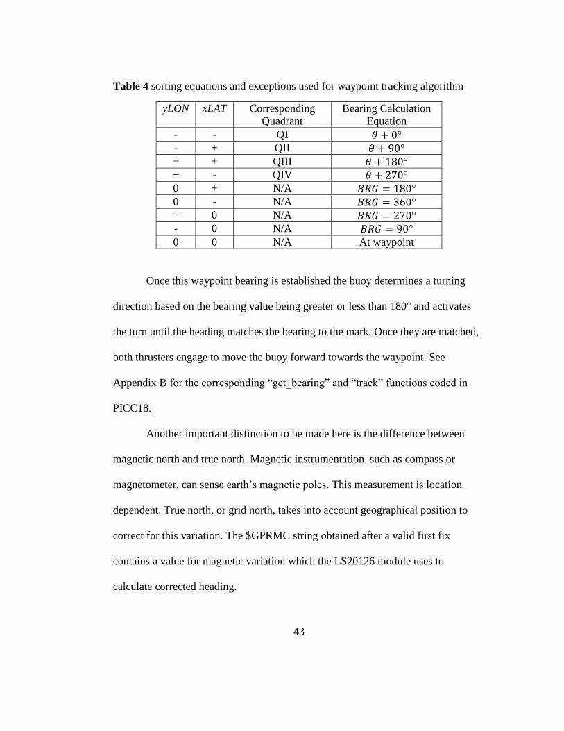
43
Table 4 sorting equations and exceptions used for waypoint tracking algorithm
yLON xLAT Corresponding
Quadrant
Bearing Calculation
Equation
- - QI
- + QII
+ + QIII
+ - QIV
0 + N/A
0 - N/A
+ 0 N/A
- 0 N/A
0 0 N/A At waypoint
Once this waypoint bearing is established the buoy determines a turning
direction based on the bearing value being greater or less than 180° and activates
the turn until the heading matches the bearing to the mark. Once they are matched,
both thrusters engage to move the buoy forward towards the waypoint. See
Appendix B for the corresponding “get_bearing” and “track” functions coded in
PICC18.
Another important distinction to be made here is the difference between
magnetic north and true north. Magnetic instrumentation, such as compass or
magnetometer, can sense earth’s magnetic poles. This measurement is location
dependent. True north, or grid north, takes into account geographical position to
correct for this variation. The $GPRMC string obtained after a valid first fix
contains a value for magnetic variation which the LS20126 module uses to
calculate corrected heading.
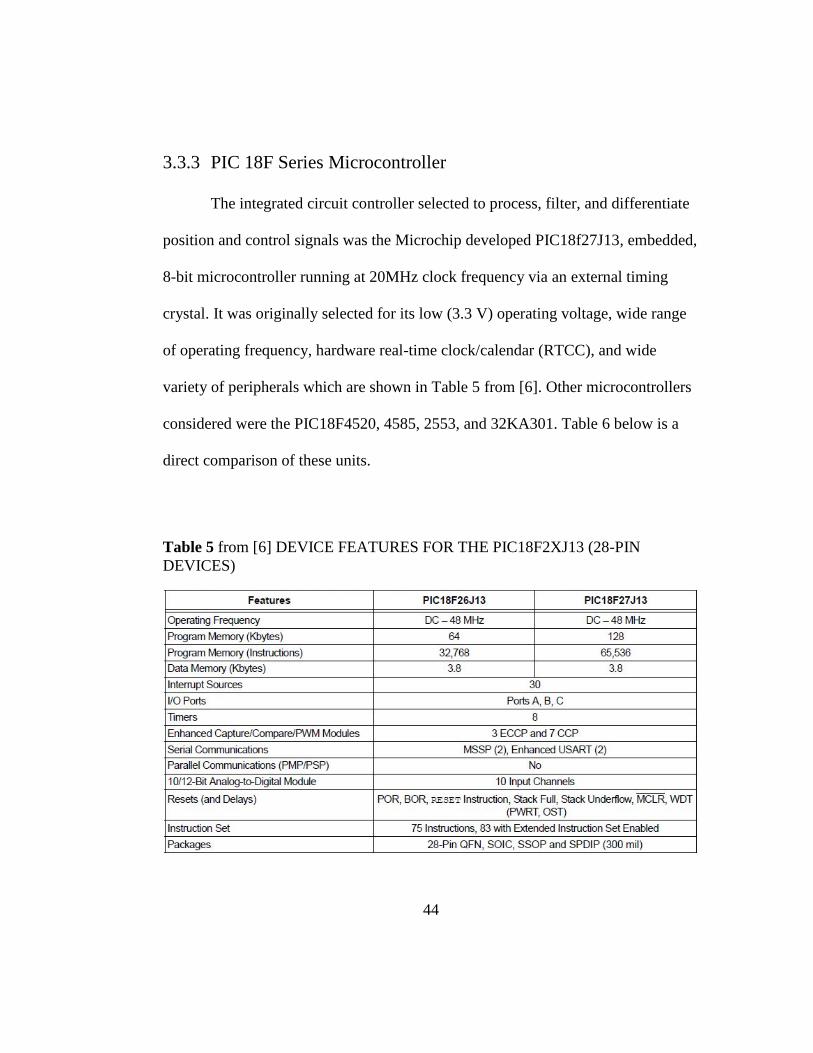
44
3.3.3 PIC 18F Series Microcontroller
The integrated circuit controller selected to process, filter, and differentiate
position and control signals was the Microchip developed PIC18f27J13, embedded,
8-bit microcontroller running at 20MHz clock frequency via an external timing
crystal. It was originally selected for its low (3.3 V) operating voltage, wide range
of operating frequency, hardware real-time clock/calendar (RTCC), and wide
variety of peripherals which are shown in Table 5 from [6]. Other microcontrollers
considered were the PIC18F4520, 4585, 2553, and 32KA301. Table 6 below is a
direct comparison of these units.
Table 5 from [6] DEVICE FEATURES FOR THE PIC18F2XJ13 (28-PIN
DEVICES)
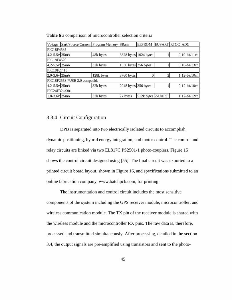
45
Table 6 a comparison of microcontroller selection criteria
3.3.4 Circuit Configuration
DPB is separated into two electrically isolated circuits to accomplish
dynamic positioning, hybrid energy integration, and motor control. The control and
relay circuits are linked via two EL817C PS2501-1 photo-couplers. Figure 15
shows the control circuit designed using [55]. The final circuit was exported to a
printed circuit board layout, shown in Figure 16, and specifications submitted to an
online fabrication company, www.batchpcb.com, for printing.
The instrumentation and control circuit includes the most sensitive
components of the system including the GPS receiver module, microcontroller, and
wireless communication module. The TX pin of the receiver module is shared with
the wireless module and the microcontroller RX pins. The raw data is, therefore,
processed and transmitted simultaneously. After processing, detailed in the section
3.4, the output signals are pre-amplified using transistors and sent to the photo-
Voltage Sink/Source Current Program Memory SRam EEPROM EUSART RTCC ADC
4.2-5.5v 25mA 48k bytes 3328 bytes 1024 bytes 1 0 10-bit/11ch
4.2-5.5v 25mA 32k bytes 1536 bytes 256 bytes 1 0 10-bit/13ch
2.0-3.6v 25mA 128k bytes 3760 bytes 0 2 1 12-bit/10ch
4.2-5.5v 25mA 32k bytes 2048 bytes 256 bytes 1 0 12-bit/10ch
1.8-3.6v 25mA 32k bytes 2k bytes 512k bytes 2-UART 1 12-bit/12ch
PIC18F4585
PIC18F4520
PIC18F27j13
PIC18F2553 *USB 2.0 compatible
PIC24F32ka301
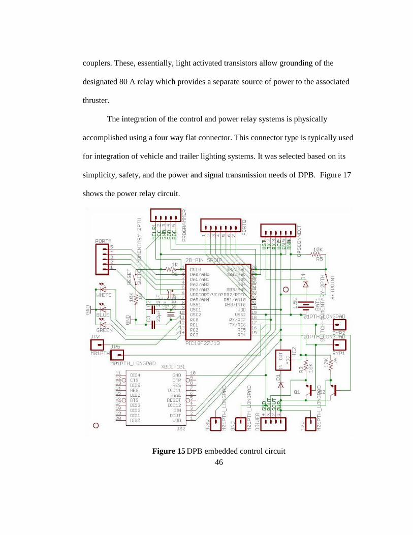
46
couplers. These, essentially, light activated transistors allow grounding of the
designated 80 A relay which provides a separate source of power to the associated
thruster.
The integration of the control and power relay systems is physically
accomplished using a four way flat connector. This connector type is typically used
for integration of vehicle and trailer lighting systems. It was selected based on its
simplicity, safety, and the power and signal transmission needs of DPB. Figure 17
shows the power relay circuit.
Figure 15 DPB embedded control circuit
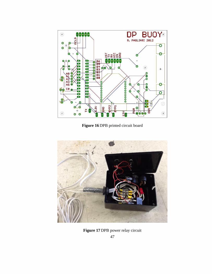
47
Figure 16 DPB printed circuit board
Figure 17 DPB power relay circuit

48
3.3.5 AndroidTM
Smart Phone
The Android smart phone is a multi-purpose, hand held, device that is in
widespread use among consumers. It allows users to stay connected to the internet
as well as stay in contact over cellular frequency. The Android OS uses a Linux
kernel to run modular applications on the device that range anywhere from
interactive calendars to gaming.
Its popularity can be partly attributed to the open source paradigm in which
it follows. This allows any user the ability to design and market his or her, content-
rich, applications using any combination of pre-installed hardware peripherals and
services. Typical peripherals, at a minimum, include cellular module, Wifi and
Bluetooth wireless modules, GPS receiver, cameras, accelerometer, and storage.
The shocnet application, discussed in section 3.4.2, makes use of the Wifi and
storage peripherals for communication with and remote control of DPB.
3.4 Software and Application
Two primary software packages were developed for DPB. Embedded
systems code, DPBfinal.c, was written with [47] and [48] and mobile wireless
communication and control application, shocnet, was written with DPB using [49].
49
3.4.1 Embedded Systems and Pseudo Dynamic Positioning
The DPB communication and control functions saved in flash ROM on the
microcontroller interact with the LS20126 and RN-XV modules as well as the
trolling motor relays, to drive DPB in both manual and auto modes of operation.
The default mode of operation for DPB on start up is manual. After
initialization, the main() function calls manual_control() which listens for a signal
input from the RN-XV module on port B. Corresponding output signals are then
distributed from port C to activate either the port, starboard, or both motors for
steering, and to set DPB into auto tracking mode. For local control the user push
button switch signals are sent directly to the relays, bypassing the controller
entirely.
When activated, auto mode calls the get_position() function storing the
current latitude and longitude coordinates, the setpoint, to memory. Get_position is
a function which communicates with the GPS module via RS-232 USART, at a rate
of 9600 baud, using 8 data bits, 1 stop bit, and no parity to acquire raw NMEA
strings. It is also a parsing algorithm used to assign latitude, longitude, and heading
values to integer variables whenever there is a valid position fix. When a fix is
invalid a sub function, get_heading(), is called which returns only magnetometer
heading. Filtering is also applied each iteration via a subfunction filter() within the
get_position() function. The filtered outputs are in integer format to accomodate
simple bitwise operator comparisons.
50
A noteworthy problem when capturing string arrays using the 8-bit PIC
chips is that the memory is pre-banked by default into 256 byte allocations,
therefore, limiting the number of characters that can be read into a single array
before spilling over into another bank. This is solved by combining two banks in
the linker script to increase the bank size as suggested in [29].
In auto, once the setpoint is determined, the track() function carrys out the
bulk of the positioning and control operations of DPB. The sub function
get_bearing() determines waypoint bearing using the method described in the
previous section and a simple differential control signal activates the appropriate
motor relay or relays to drive DPB back towards the set point. Figure 18 below is a
flow chart illustrating the code sequence of DPB. See Appendix B and C for the
source code listing DPBuoyFinal.c containing all functions, and
18f27j13_lrgarry.lkr containing the linker script.
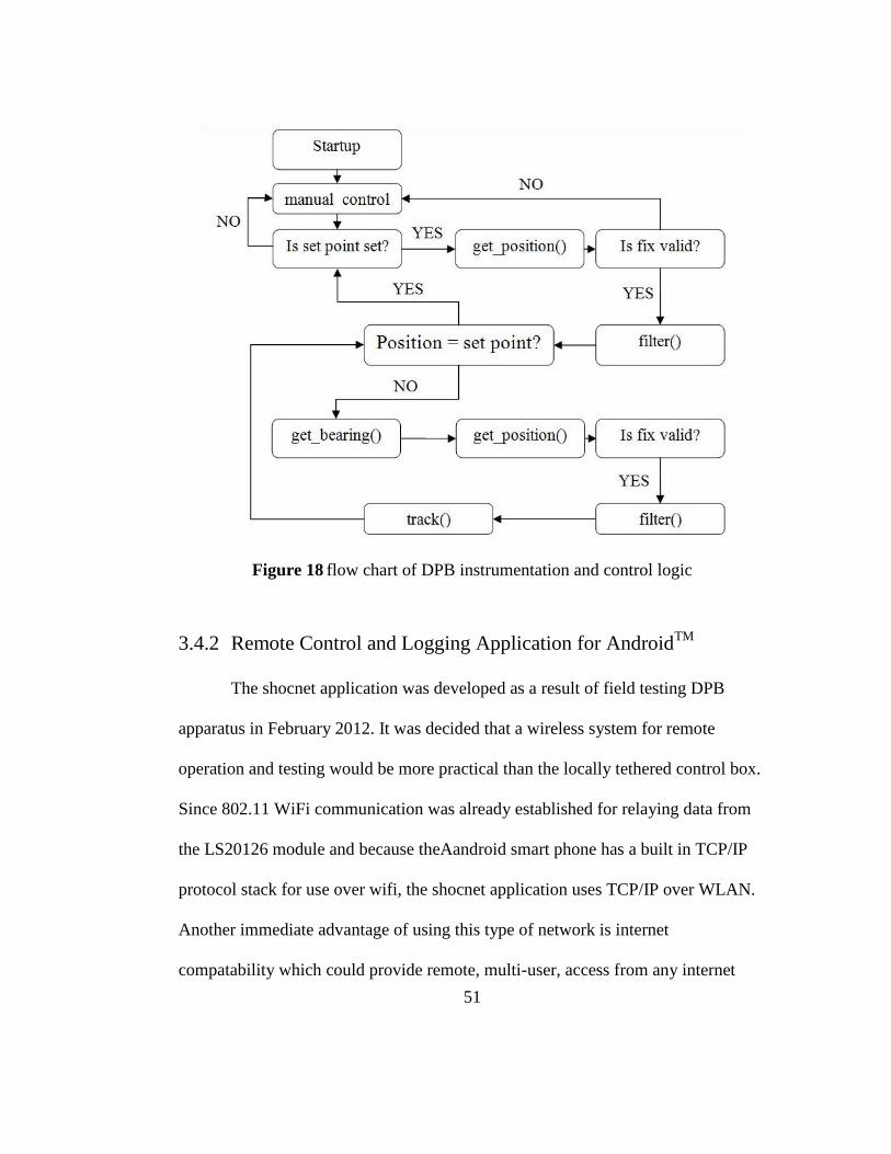
51
Figure 18 flow chart of DPB instrumentation and control logic
3.4.2 Remote Control and Logging Application for AndroidTM
The shocnet application was developed as a result of field testing DPB
apparatus in February 2012. It was decided that a wireless system for remote
operation and testing would be more practical than the locally tethered control box.
Since 802.11 WiFi communication was already established for relaying data from
the LS20126 module and because theAandroid smart phone has a built in TCP/IP
protocol stack for use over wifi, the shocnet application uses TCP/IP over WLAN.
Another immediate advantage of using this type of network is internet
compatability which could provide remote, multi-user, access from any internet
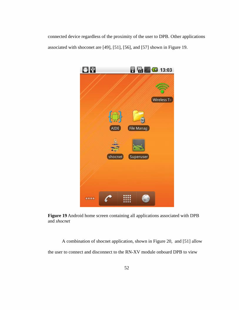
52
connected device regardless of the proximity of the user to DPB. Other applications
associated with shoconet are [49], [51], [56], and [57] shown in Figure 19.
Figure 19 Android home screen containing all applications associated with DPB
and shocnet
A combination of shocnet application, shown in Figure 20, and [51] allow
the user to connect and disconnect to the RN-XV module onboard DPB to view
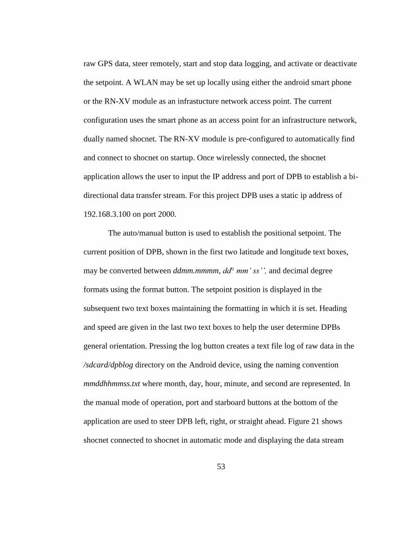
53
raw GPS data, steer remotely, start and stop data logging, and activate or deactivate
the setpoint. A WLAN may be set up locally using either the android smart phone
or the RN-XV module as an infrastucture network access point. The current
configuration uses the smart phone as an access point for an infrastructure network,
dually named shocnet. The RN-XV module is pre-configured to automatically find
and connect to shocnet on startup. Once wirelessly connected, the shocnet
application allows the user to input the IP address and port of DPB to establish a bi-
directional data transfer stream. For this project DPB uses a static ip address of
192.168.3.100 on port 2000.
The auto/manual button is used to establish the positional setpoint. The
current position of DPB, shown in the first two latitude and longitude text boxes,
may be converted between ddmm.mmmm, dd mm’ ss’’, and decimal degree
formats using the format button. The setpoint position is displayed in the
subsequent two text boxes maintaining the formatting in which it is set. Heading
and speed are given in the last two text boxes to help the user determine DPBs
general orientation. Pressing the log button creates a text file log of raw data in the
/sdcard/dpblog directory on the Android device, using the naming convention
mmddhhmmss.txt where month, day, hour, minute, and second are represented. In
the manual mode of operation, port and starboard buttons at the bottom of the
application are used to steer DPB left, right, or straight ahead. Figure 21 shows
shocnet connected to shocnet in automatic mode and displaying the data stream
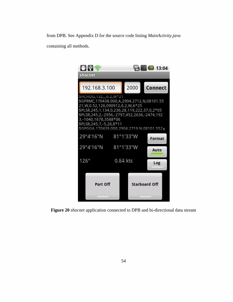
54
from DPB. See Appendix D for the source code listing MainActivity.java
containing all methods.
Figure 20 shocnet application connected to DPB and bi-directional data stream
55
4. Hybrid Renewable Energy System
To analyze the effectiveness of a renewable energy system it is important to
consider the available resources. Since the DPB operational environment is
offshore these resources include primarily wind and solar. As mentioned earlier the
unobstructed surface of the ocean is conducive to high wind velocities. Solar is also
a great resource during daylight hours, particularly at low latitudes, precluding
cloud cover. The power requirements of DPB are another important consideration
that is dependent on environmental effects. Characteristics such as duty cycle and
drag are highly affected by the total wind and surface current forces imparted on
DPB. The overall design of the hybrid renewable energy system must account for
the capabilities and the maximum loading associated with DPB. Battery storage is
also a required inclusion in the hybrid system to allow for power stability between
periods of resource shortages.
4.1 Resources
4.1.1 Wind Resources
Variable wind resources around the globe are mainly created by temperature
differentials and earth’s rotation. They follow a general circulation pattern based
on these factors. Low latitude winds between 0° and 30° are easterly, mid latitude
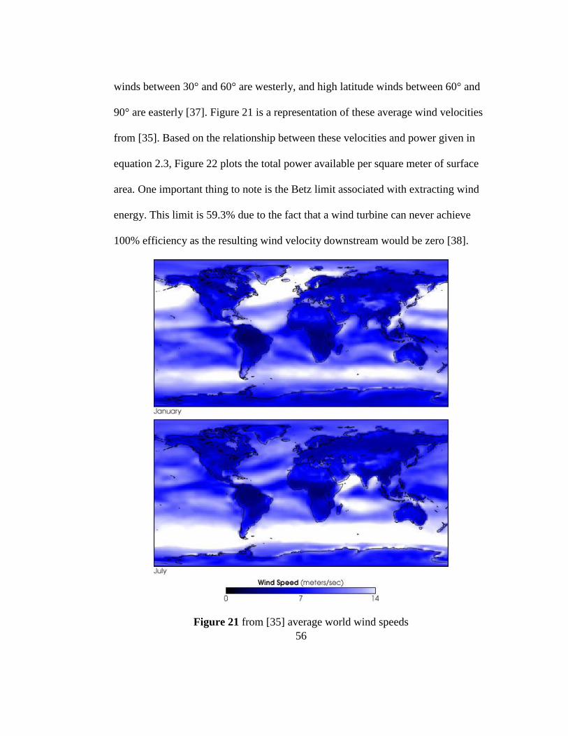
56
winds between 30° and 60° are westerly, and high latitude winds between 60° and
90° are easterly [37]. Figure 21 is a representation of these average wind velocities
from [35]. Based on the relationship between these velocities and power given in
equation 2.3, Figure 22 plots the total power available per square meter of surface
area. One important thing to note is the Betz limit associated with extracting wind
energy. This limit is 59.3% due to the fact that a wind turbine can never achieve
100% efficiency as the resulting wind velocity downstream would be zero [38].
Figure 21 from [35] average world wind speeds
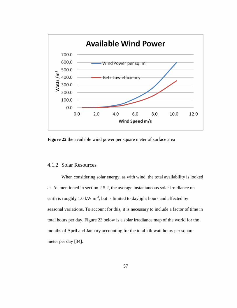
57
Figure 22 the available wind power per square meter of surface area
4.1.2 Solar Resources
When considering solar energy, as with wind, the total availability is looked
at. As mentioned in section 2.5.2, the average instantaneous solar irradiance on
earth is roughly 1.0 kW m-2
, but is limited to daylight hours and affected by
seasonal variations. To account for this, it is necessary to include a factor of time in
total hours per day. Figure 23 below is a solar irradiance map of the world for the
months of April and January accounting for the total kilowatt hours per square
meter per day [34].
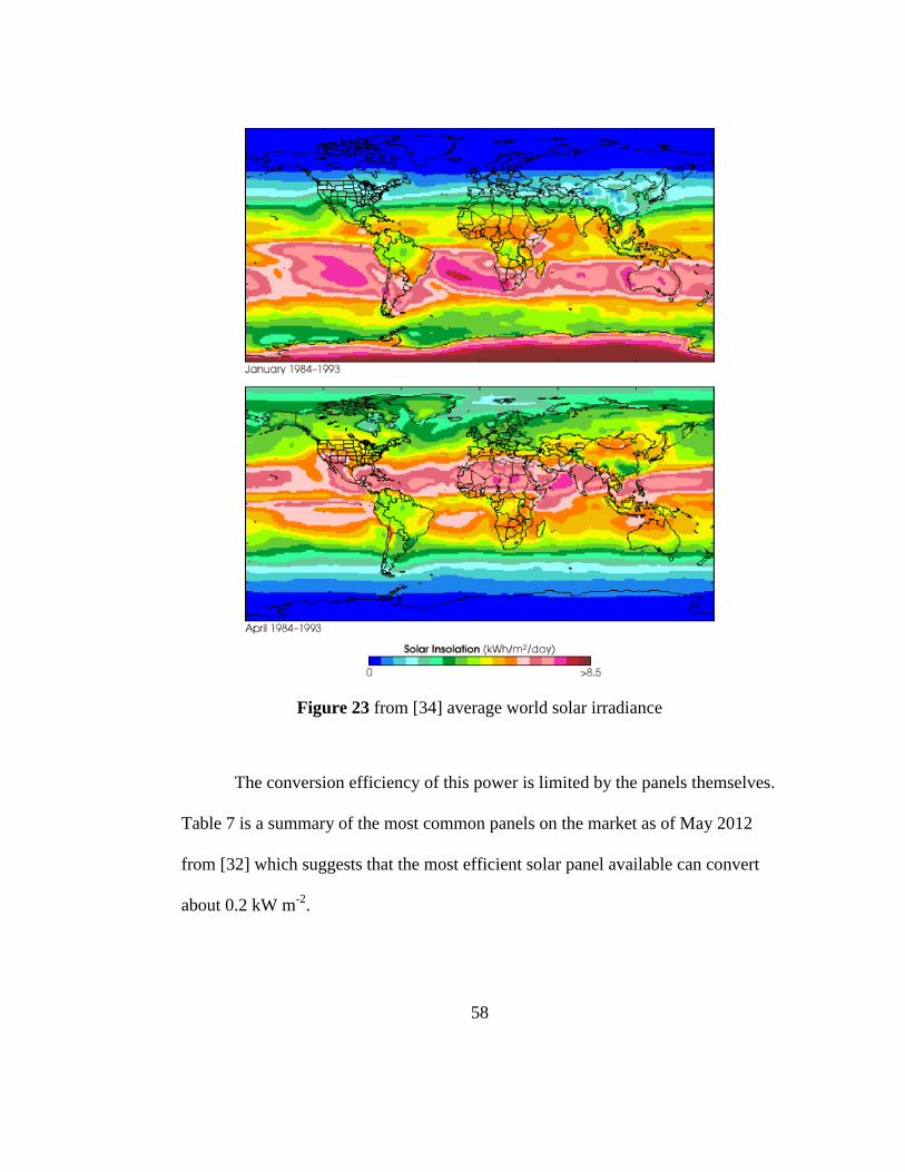
58
Figure 23 from [34] average world solar irradiance
The conversion efficiency of this power is limited by the panels themselves.
Table 7 is a summary of the most common panels on the market as of May 2012
from [32] which suggests that the most efficient solar panel available can convert
about 0.2 kW m-2
.
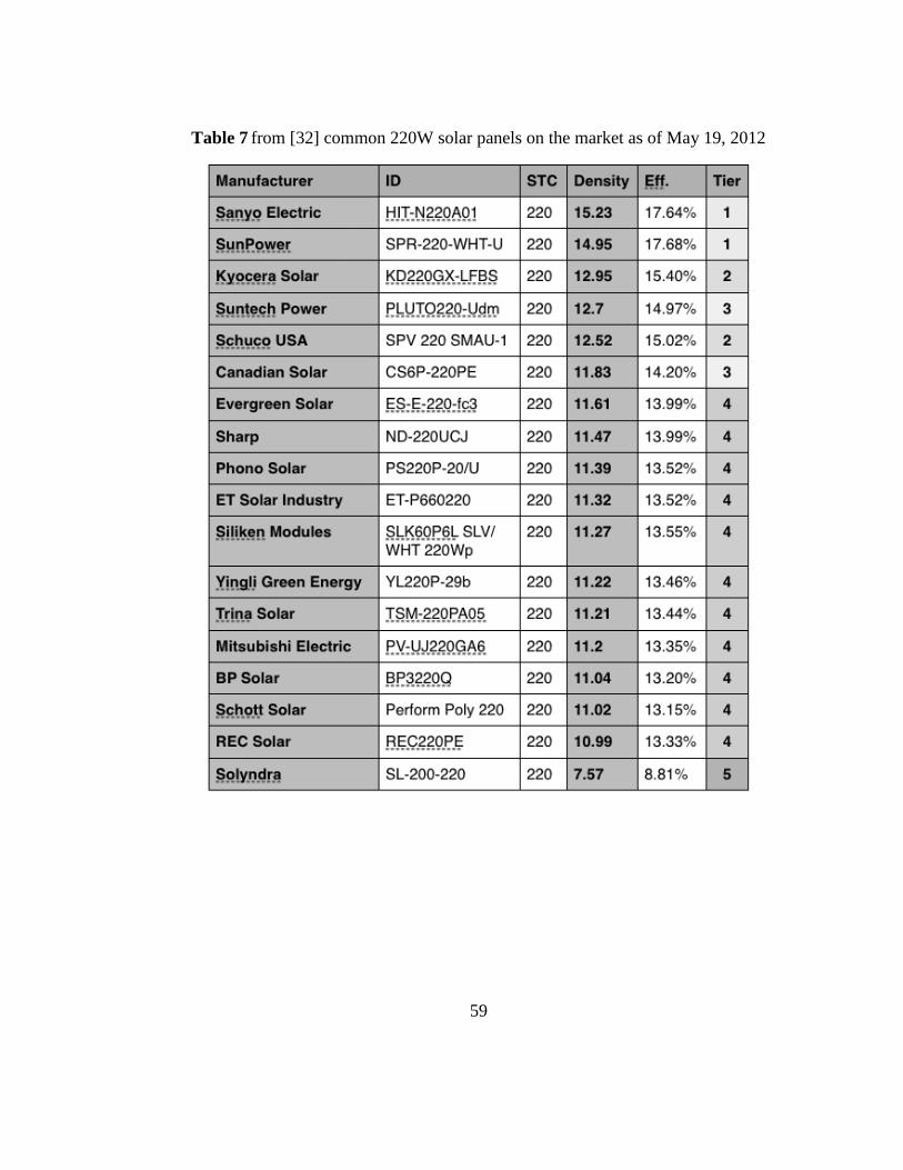
59
Table 7 from [32] common 220W solar panels on the market as of May 19, 2012
60
4.2 Loads
4.2.1 Primary Electrical Load
The primary electrical load of DPB comes from the motors associated with
positional correction. System load data was gathered from field and tank tests
detailed in section 5.1. These instantaneous power values, however, only account
for one operational environment during one instance. While this may be integrated
over a period of time to account for full loading, a load duty cycle that represents a
total expected annual run-time is used for determining the true requirements of
DPB. This duty cycle is affected by unpredictable environmental variability
throughout different locations and time. A way to account for this would involve a
long term field trial of DPB under various environmental conditions and locations.
Instead, simulations use an assumed value of 10%.
Curcio, et al. presents a detailed analysis of the ASC SCOUT, an
autonomous surface vehicle with station keeping capability, which suggests using a
10% propulsive duty cycle for station keeping [28]. At 100% loading, DPB
requirements would correlate to approximately 30 kWh per day. At this high value,
the likelihood of a renewable energy system is improbable. A 10% duty cycle gives
a more practical 3.1 kWh per day value.

61
4.2.2 Control System Electrical Load
The major control system loads for DPB are from the GPS module, PIC18
series microcontroller, and wireless module. A listing of control system loads is
given in Table 8 below.
Table 8 Instrumentation and control system loads
Unit Specifications Peak Power Steady State
LS20126 Module 587 mW 102 mW
PIC18F27J13 Microcontroller 64 mW 33 mW
RN-XV Wireless Module 594 mW 123 mW
Total Loads from Data sheets 1.2 W 0.25 W
Actual Measured Loads 3.4 W 2.9W
It was concluded these maximum power requirements for the DPB
instrumentation and control system are negligible when compared to the power
requirements of the propulsion system and considering the nominal power capacity
of the hybrid energy system.
4.3 Hybrid Energy System Design
4.3.1 Hybrid Optimization Model for Electric Renewables (HOMER)
Hybrid Optimization Model for Electric Renewables (HOMER) is the
power systems modeling and analysis tool that was used for renewable energy
system design simulations on DPB. It was selected because the software’s legacy

62
version is freely distributed and offers both standalone as well as grid tied system
modeling capabilities.
HOMER was developed by the National Renewable Energy Lab (NREL) in
the 1990’s as an internal modeling program used to, “Understand the design trade-
offs between different systems configurations [36].” The software allows analysis
of several hybrid energy system configurations based on inputs of environmental
resource data and renewable energy components. Results from the simulations
made at four different locations around the world suggest that the hybrid energy
system could be feasible, pending advancements in energy storage technology.
Inputs to [54] include the solar and wind resources imported from [2] and
[63], along with the selected renewable energy system components. These were
entered manually and based on performance characteristics of available solar panels
and wind turbines. Considerations for the renewable energy system components
were size restrictions, based on space available on the buoy, weight, and total
power requirements of DPB.
Two sets of solar panels were included in the analysis. One set was the
Sanyo Electric 225 W mono crystalline/amorphous silicon hybrid panel (HIT-
N225A01) from Solarsystems USA online at www.solarsystemsUSA.net. These
cost $606.38 and weigh 16 kg each. They have a power density of 209.1 W m-2
or
17.8% module efficiency. The panel dimensions are 158 cm X 80 cm X 4.6 cm.
Another set was the ET Solar 95 Watt mono crystalline panels (ET-M53695, 95/36)
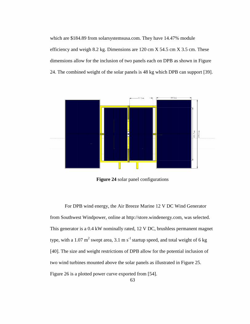
63
which are $184.89 from solarsystemsusa.com. They have 14.47% module
efficiency and weigh 8.2 kg. Dimensions are 120 cm X 54.5 cm X 3.5 cm. These
dimensions allow for the inclusion of two panels each on DPB as shown in Figure
24. The combined weight of the solar panels is 48 kg which DPB can support [39].
Figure 24 solar panel configurations
For DPB wind energy, the Air Breeze Marine 12 V DC Wind Generator
from Southwest Windpower, online at http://store.windenergy.com, was selected.
This generator is a 0.4 kW nominally rated, 12 V DC, brushless permanent magnet
type, with a 1.07 m2 swept area, 3.1 m s
-1 startup speed, and total weight of 6 kg
[40]. The size and weight restrictions of DPB allow for the potential inclusion of
two wind turbines mounted above the solar panels as illustrated in Figure 25.
Figure 26 is a plotted power curve exported from [54].
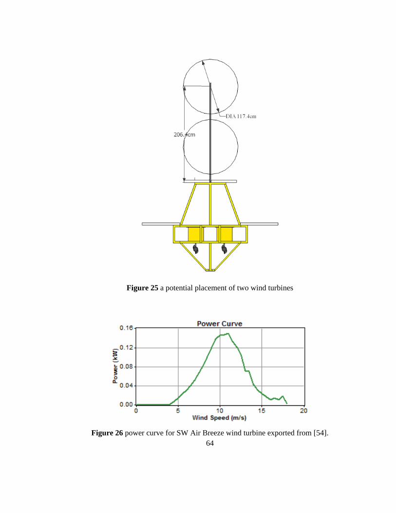
64
Figure 25 a potential placement of two wind turbines
Figure 26 power curve for SW Air Breeze wind turbine exported from [54].
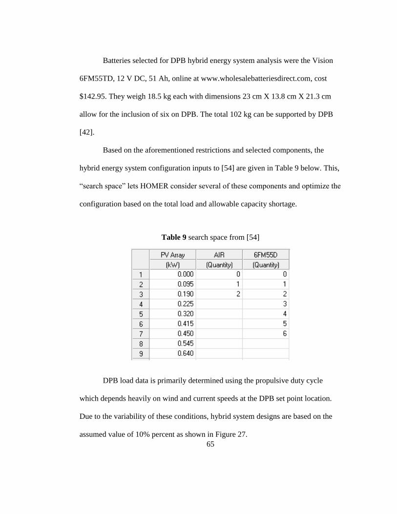
65
Batteries selected for DPB hybrid energy system analysis were the Vision
6FM55TD, 12 V DC, 51 Ah, online at www.wholesalebatteriesdirect.com, cost
$142.95. They weigh 18.5 kg each with dimensions 23 cm X 13.8 cm X 21.3 cm
allow for the inclusion of six on DPB. The total 102 kg can be supported by DPB
[42].
Based on the aforementioned restrictions and selected components, the
hybrid energy system configuration inputs to [54] are given in Table 9 below. This,
“search space” lets HOMER consider several of these components and optimize the
configuration based on the total load and allowable capacity shortage.
Table 9 search space from [54]
DPB load data is primarily determined using the propulsive duty cycle
which depends heavily on wind and current speeds at the DPB set point location.
Due to the variability of these conditions, hybrid system designs are based on the
assumed value of 10% percent as shown in Figure 27.
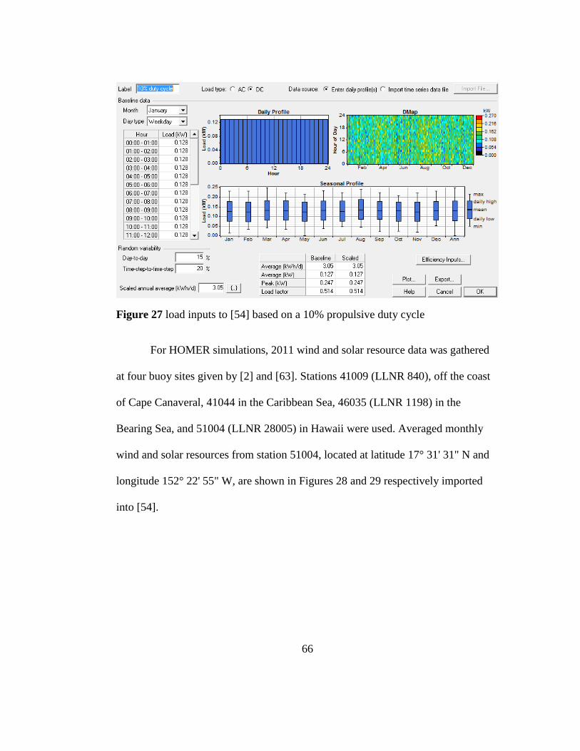
66
Figure 27 load inputs to [54] based on a 10% propulsive duty cycle
For HOMER simulations, 2011 wind and solar resource data was gathered
at four buoy sites given by [2] and [63]. Stations 41009 (LLNR 840), off the coast
of Cape Canaveral, 41044 in the Caribbean Sea, 46035 (LLNR 1198) in the
Bearing Sea, and 51004 (LLNR 28005) in Hawaii were used. Averaged monthly
wind and solar resources from station 51004, located at latitude 17° 31' 31" N and
longitude 152° 22' 55" W, are shown in Figures 28 and 29 respectively imported
into [54].
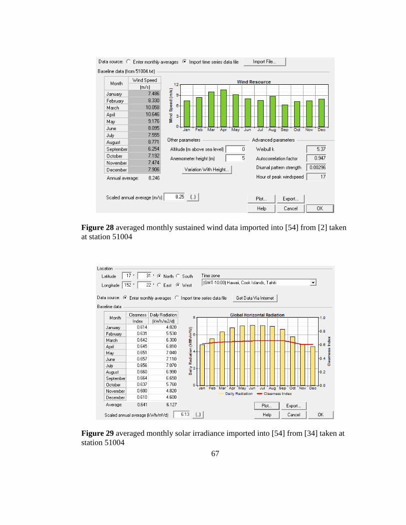
67
Figure 28 averaged monthly sustained wind data imported into [54] from [2] taken
at station 51004
Figure 29 averaged monthly solar irradiance imported into [54] from [34] taken at
station 51004

68
4.3.2 Simulation Results
Interpretation of the results from HOMER requires the identification of load
shedding conditions and capacity shortage. Load shedding occurs when the energy
demand exceeds generated power placing energy storage in a discharge state.
Capacity shortage is the fraction of load shedding that exceeds the total capacity of
the hybrid system. This fraction is used as the ultimate determination of whether or
not the hybrid renewable energy system will work for DPB [54].
Simulation results from station 51004 are presented in Figure 30 which
revealed the most promising solutions. They indicated that the optimum wind and
solar hybrid energy system configuration for DPB, if located in the southeastern
Hawaiian Islands, could sustain load requirements with less than a 1% annual
capacity shortage. Results from station 46035 had the highest capacity shortage of
38%.
Stations 41009 and 41044 simulations suggest that seasonal variability of
renewable energy resources such as light winds during the summer months may be
a leading contributor to the capacity shortage at these Florida and Caribbean sites.
Battery storage capacity was identified as the most considerable restriction for the
hybrid energy systems in these cases. In order to cover these shortages the battery
storage capacity would have to include approximately 1,700 Ah or 31 batteries.
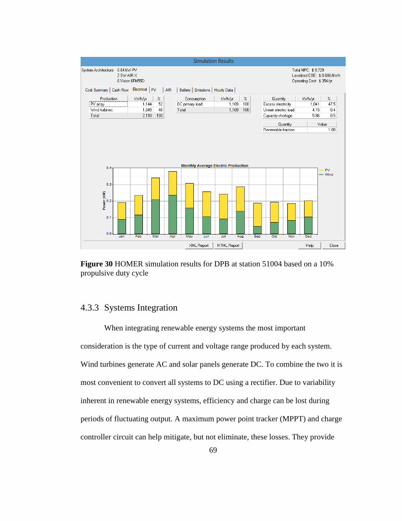
69
Figure 30 HOMER simulation results for DPB at station 51004 based on a 10%
propulsive duty cycle
4.3.3 Systems Integration
When integrating renewable energy systems the most important
consideration is the type of current and voltage range produced by each system.
Wind turbines generate AC and solar panels generate DC. To combine the two it is
most convenient to convert all systems to DC using a rectifier. Due to variability
inherent in renewable energy systems, efficiency and charge can be lost during
periods of fluctuating output. A maximum power point tracker (MPPT) and charge
controller circuit can help mitigate, but not eliminate, these losses. They provide
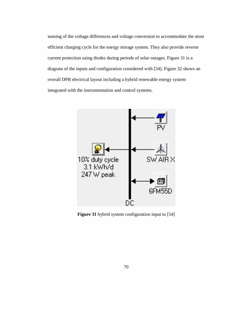
70
sensing of the voltage differences and voltage conversion to accommodate the most
efficient charging cycle for the energy storage system. They also provide reverse
current protection using diodes during periods of solar outages. Figure 31 is a
diagram of the inputs and configuration considered with [54]. Figure 32 shows an
overall DPB electrical layout including a hybrid renewable energy system
integrated with the instrumentation and control systems.
Figure 31 hybrid system configuration input to [54]
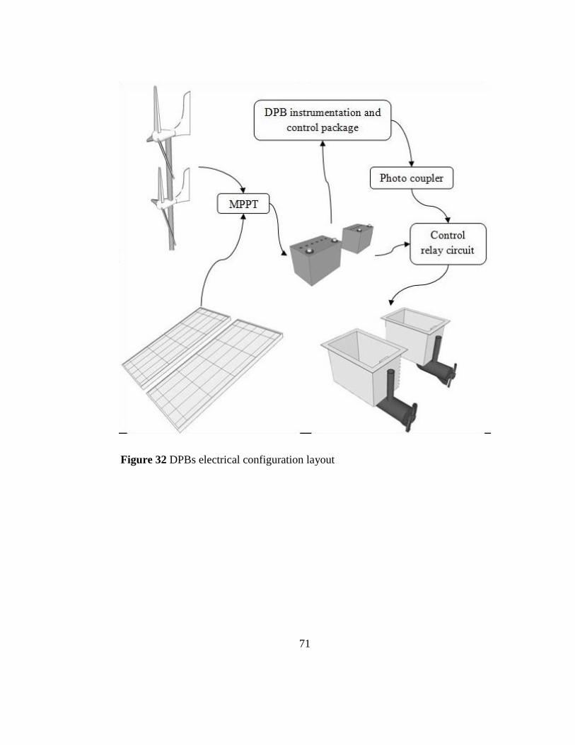
71
Figure 32 DPBs electrical configuration layout
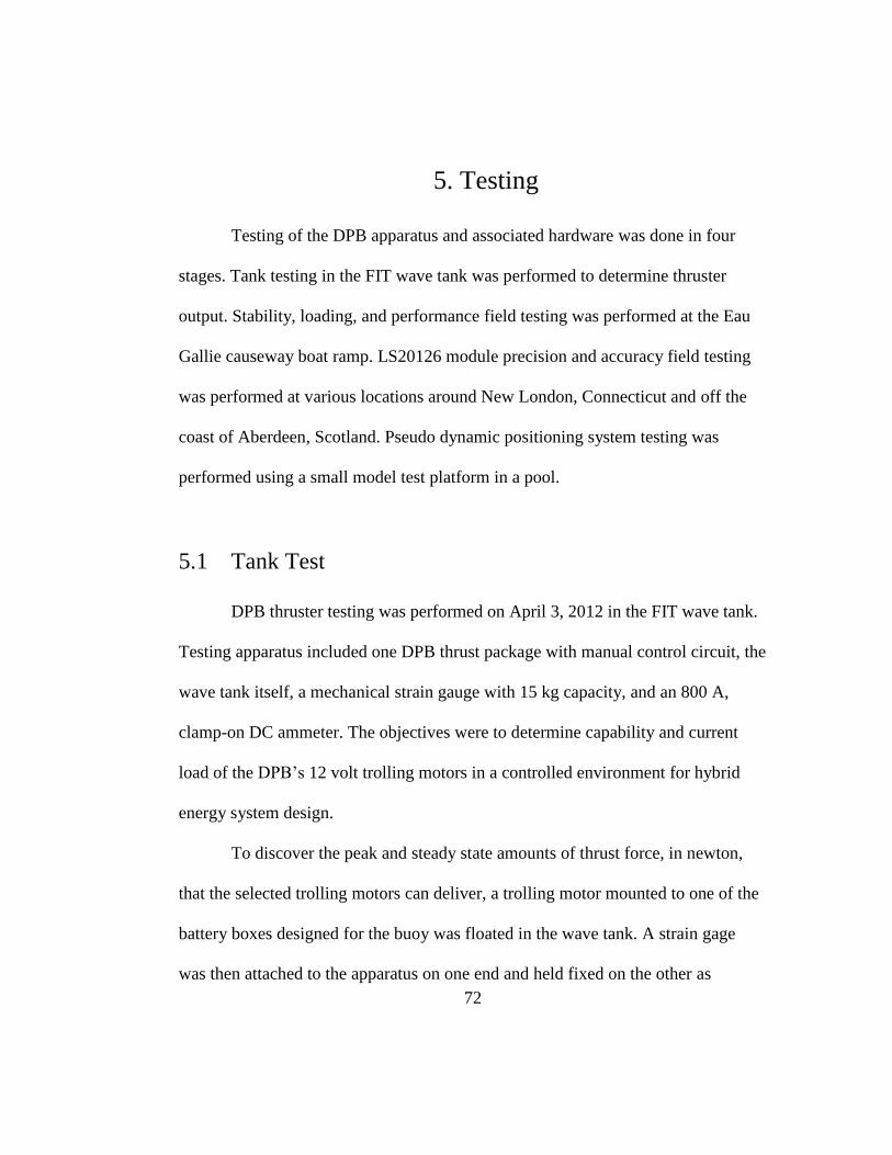
72
5. Testing
Testing of the DPB apparatus and associated hardware was done in four
stages. Tank testing in the FIT wave tank was performed to determine thruster
output. Stability, loading, and performance field testing was performed at the Eau
Gallie causeway boat ramp. LS20126 module precision and accuracy field testing
was performed at various locations around New London, Connecticut and off the
coast of Aberdeen, Scotland. Pseudo dynamic positioning system testing was
performed using a small model test platform in a pool.
5.1 Tank Test
DPB thruster testing was performed on April 3, 2012 in the FIT wave tank.
Testing apparatus included one DPB thrust package with manual control circuit, the
wave tank itself, a mechanical strain gauge with 15 kg capacity, and an 800 A,
clamp-on DC ammeter. The objectives were to determine capability and current
load of the DPB’s 12 volt trolling motors in a controlled environment for hybrid
energy system design.
To discover the peak and steady state amounts of thrust force, in newton,
that the selected trolling motors can deliver, a trolling motor mounted to one of the
battery boxes designed for the buoy was floated in the wave tank. A strain gage
was then attached to the apparatus on one end and held fixed on the other as
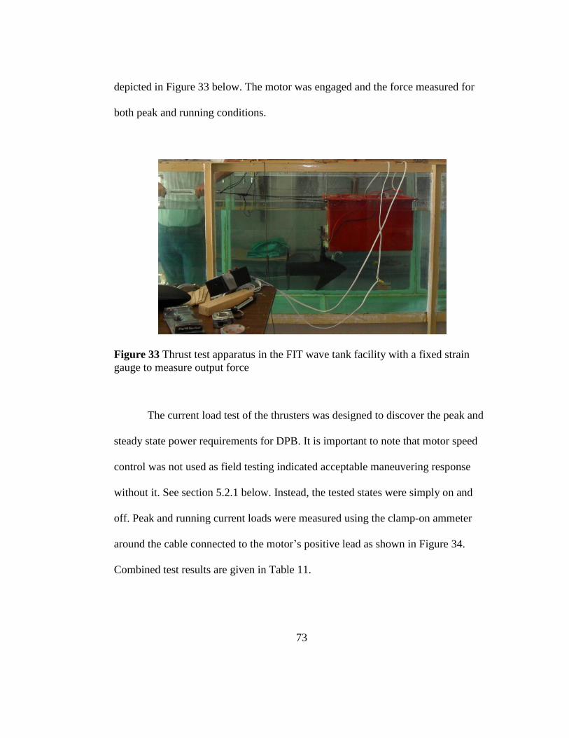
73
depicted in Figure 33 below. The motor was engaged and the force measured for
both peak and running conditions.
Figure 33 Thrust test apparatus in the FIT wave tank facility with a fixed strain
gauge to measure output force
The current load test of the thrusters was designed to discover the peak and
steady state power requirements for DPB. It is important to note that motor speed
control was not used as field testing indicated acceptable maneuvering response
without it. See section 5.2.1 below. Instead, the tested states were simply on and
off. Peak and running current loads were measured using the clamp-on ammeter
around the cable connected to the motor’s positive lead as shown in Figure 34.
Combined test results are given in Table 11.
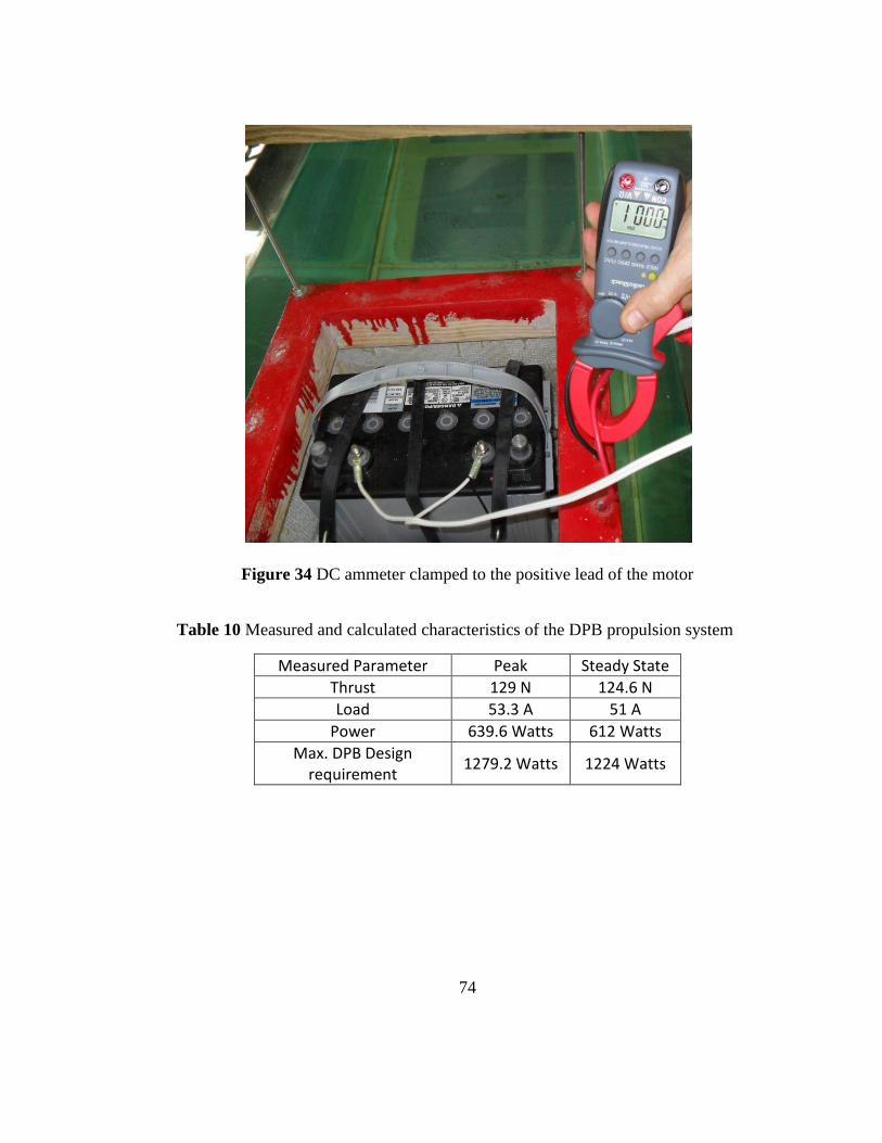
74
Figure 34 DC ammeter clamped to the positive lead of the motor
Table 10 Measured and calculated characteristics of the DPB propulsion system
Measured Parameter Peak Steady State
Thrust 129 N 124.6 N
Load 53.3 A 51 A
Power 639.6 Watts 612 Watts
Max. DPB Design requirement
1279.2 Watts 1224 Watts
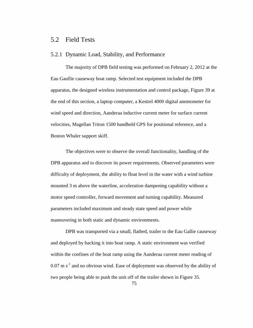
75
5.2 Field Tests
5.2.1 Dynamic Load, Stability, and Performance
The majority of DPB field testing was performed on February 2, 2012 at the
Eau Gaullie causeway boat ramp. Selected test equipment included the DPB
apparatus, the designed wireless instrumentation and control package, Figure 39 at
the end of this section, a laptop computer, a Kestrel 4000 digital anemometer for
wind speed and direction, Aanderaa inductive current meter for surface current
velocities, Magellan Triton 1500 handheld GPS for positional reference, and a
Boston Whaler support skiff.
The objectives were to observe the overall functionality, handling of the
DPB apparatus and to discover its power requirements. Observed parameters were
difficulty of deployment, the ability to float level in the water with a wind turbine
mounted 3 m above the waterline, acceleration dampening capability without a
motor speed controller, forward movement and turning capability. Measured
parameters included maximum and steady state speed and power while
maneuvering in both static and dynamic environments.
DPB was transported via a small, flatbed, trailer to the Eau Gallie causeway
and deployed by backing it into boat ramp. A static environment was verified
within the confines of the boat ramp using the Aanderaa current meter reading of
0.07 m s-1
and no obvious wind. Ease of deployment was observed by the ability of
two people being able to push the unit off of the trailer shown in Figure 35.
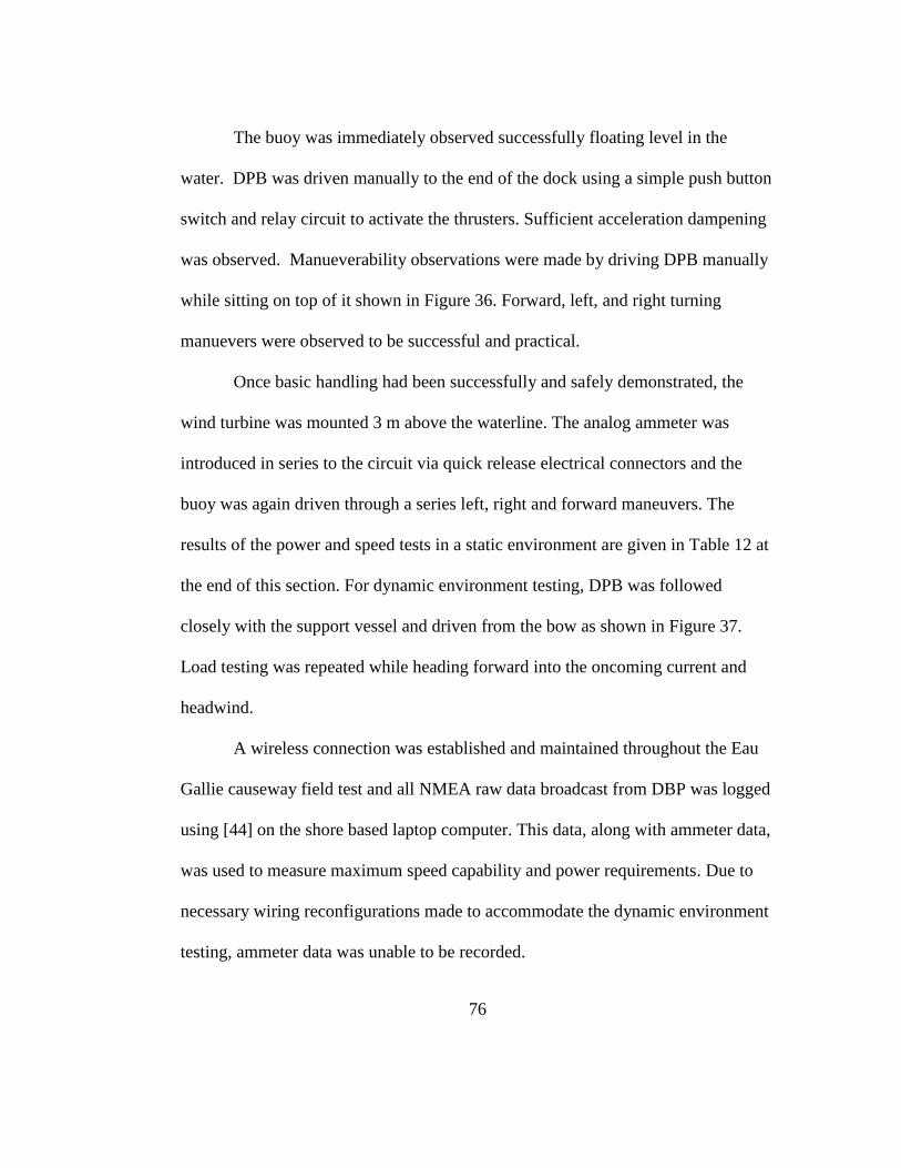
76
The buoy was immediately observed successfully floating level in the
water. DPB was driven manually to the end of the dock using a simple push button
switch and relay circuit to activate the thrusters. Sufficient acceleration dampening
was observed. Manueverability observations were made by driving DPB manually
while sitting on top of it shown in Figure 36. Forward, left, and right turning
manuevers were observed to be successful and practical.
Once basic handling had been successfully and safely demonstrated, the
wind turbine was mounted 3 m above the waterline. The analog ammeter was
introduced in series to the circuit via quick release electrical connectors and the
buoy was again driven through a series left, right and forward maneuvers. The
results of the power and speed tests in a static environment are given in Table 12 at
the end of this section. For dynamic environment testing, DPB was followed
closely with the support vessel and driven from the bow as shown in Figure 37.
Load testing was repeated while heading forward into the oncoming current and
headwind.
A wireless connection was established and maintained throughout the Eau
Gallie causeway field test and all NMEA raw data broadcast from DBP was logged
using [44] on the shore based laptop computer. This data, along with ammeter data,
was used to measure maximum speed capability and power requirements. Due to
necessary wiring reconfigurations made to accommodate the dynamic environment
testing, ammeter data was unable to be recorded.
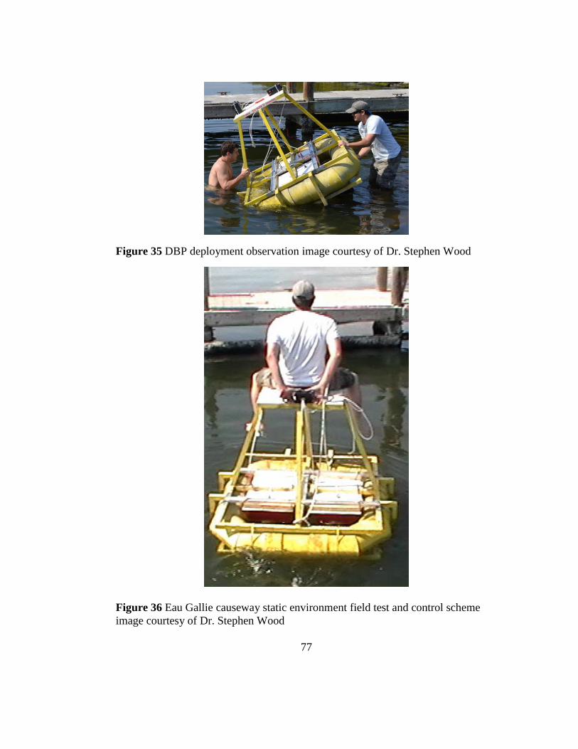
77
Figure 35 DBP deployment observation image courtesy of Dr. Stephen Wood
Figure 36 Eau Gallie causeway static environment field test and control scheme
image courtesy of Dr. Stephen Wood
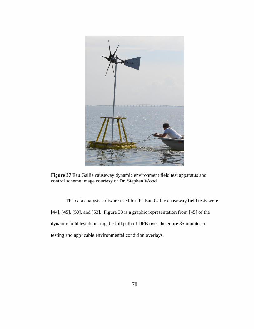
78
Figure 37 Eau Gallie causeway dynamic environment field test apparatus and
control scheme image courtesy of Dr. Stephen Wood
The data analysis software used for the Eau Gallie causeway field tests were
[44], [45], [50], and [53]. Figure 38 is a graphic representation from [45] of the
dynamic field test depicting the full path of DPB over the entire 35 minutes of
testing and applicable environmental condition overlays.
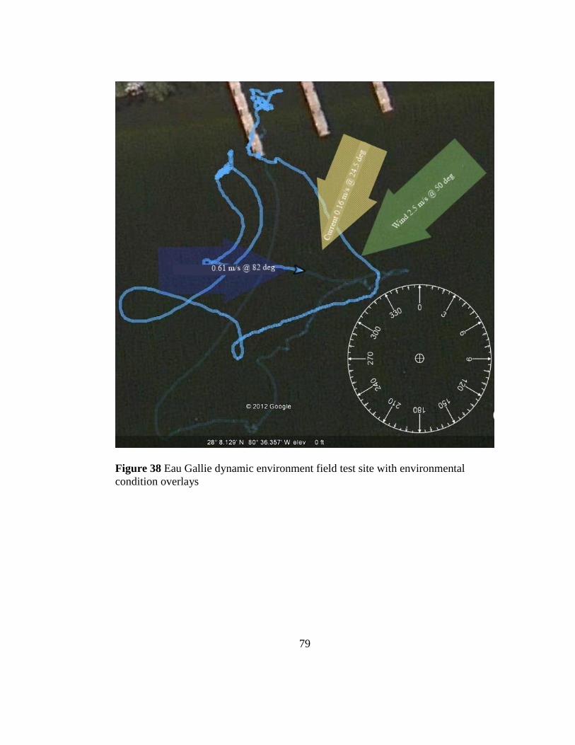
79
Figure 38 Eau Gallie dynamic environment field test site with environmental
condition overlays
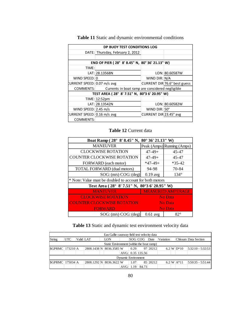
80
Table 11 Static and dynamic environmental conditions
Table 12 Current data
Table 13 Static and dynamic test environment velocity data
DATE: Thursday, February 2, 2012
TIME:
LAT: 28.13568N LON: 80.60587W
WIND SPEED: 0 WIND DIR: N/A
CURRENT SPEED: 0.07 m/s avg CURRENT DIR:76.6° best guess
COMMENTS:
TIME: 12:52pm
LAT: 28.13542N LON: 80.60582W
WIND SPEED: 2.45 m/s WIND DIR: 50°
CURRENT SPEED: 0.16 m/s avg CURRENT DIR:23.45° avg
COMMENTS:
DP BUOY TEST CONDITIONS LOG
END OF PIER ( 28° 8' 8.45" N, 80° 36' 21.13" W)
Currents in boat ramp are considered negligible
TEST AREA ( 28° 8' 7.51" N, 80°3 6' 20.95" W)
Peak (Amps) Running (Amps)
47-49+ 45-47
47-49+ 45-47
*47-49+ *35-42
94-98 70-84
0.19 avg 134°
0.61 avg 82°SOG: (m/s) COG: (deg)
CLOCKWISE ROTATION No Data
COUNTER CLOCKWISE ROTATION No Data
FORWARD No Data
TOTAL FORWARD (dual motors)
SOG: (m/s) COG: (deg)
Test Area ( 28° 8' 7.51" N, 80°3 6' 20.95" W)
MANEUVER MEASURED AMPERAGE
* Note: Value must be doubled to account for both motors
Boat Ramp ( 28° 8' 8.45" N, 80° 36' 21.13" W)
MANEUVER
CLOCKWISE ROTATION
COUNTER CLOCKWISE ROTATION
FORWARD (each motor)
String UTC Valid LAT LON SOG COG Date Variation Chksum Data Section
$GPRMC 173210 A 2808.1438 N 8036.3585 W 0.29 97 20212 6.2 W D*10 5:32:10 - 5:32:53
AVG: 0.35 135.56
$GPRMC 175034 A 2808.1292 N 8036.3622 W 1.07 85 20212 6.2 W A*11 5:50:35 - 5:51:44
AVG: 1.19 84.73
Eau Gallie causway field test velocity data
Static Environment (within the boat ramp)
Dynamic Environment
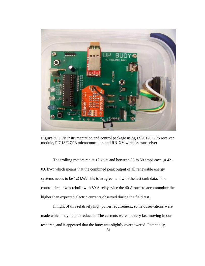
81
Figure 39 DPB instrumentation and control package using LS20126 GPS receiver
module, PIC18F27j13 microcontroller, and RN-XV wireless transceiver
The trolling motors ran at 12 volts and between 35 to 50 amps each (0.42 -
0.6 kW) which means that the combined peak output of all renewable energy
systems needs to be 1.2 kW. This is in agreement with the test tank data. The
control circuit was rebuilt with 80 A relays vice the 40 A ones to accommodate the
higher than expected electric currents observed during the field test.
In light of this relatively high power requirement, some observations were
made which may help to reduce it. The currents were not very fast moving in our
test area, and it appeared that the buoy was slightly overpowered. Potentially,

82
smaller or more efficient motors could be used to minimize the power requirements
and still hold the buoy on station. Additional power requirements could be met by
adding an additional wind turbine.
5.2.2 Form Drag Analysis from Dynamic Field Test
For completeness the drag force for DPB is calculated using an assumed
drag coefficient, values obtained from the DPB tank and field tests, and cross
sections shown in Figures 41 and 42. Based on this result, the form drag curves are
extrapolated using the drag equation 5.1 and are given in Figure 40.
Assumptions include steady, irrotational, and incompressible flow for
water. Due to low average air velocities below 2.5 m s-1
resulting in Mach numbers
less than 0.3, air may also be treated as incompressible as suggested by [58]. Only
the x component of apparent velocities, averaged over the given test sample, are
used for simplification of force calculations. Wave drag is neglected due to
insignificant wave heights observed during testing. All values are converted to
metric for consistency. The drag equation, 5.1 below, was taken from [58]. All
assumed values were taken from [58] and [60].
Where is the drag force on the buoy resulting from the respective fluid, ρ is
density given as 1027 kg m-3
for seawater and 1.16 kg m-3
for air at sea level, v is
the average apparent velocity of 0.77 m s-1
for water current and 2.51 m s-1
for
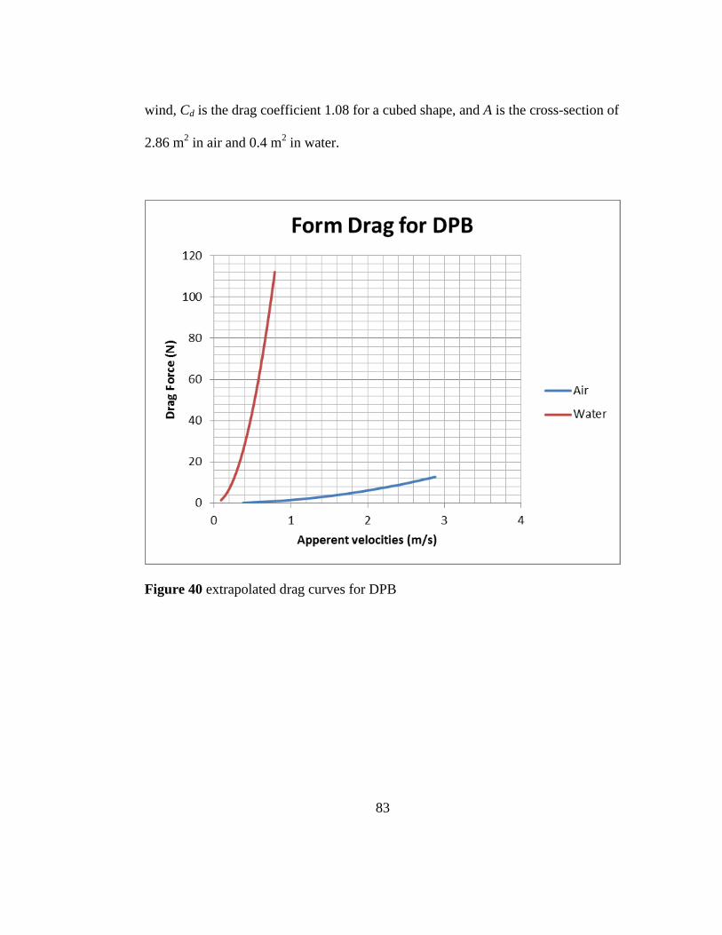
83
wind, Cd is the drag coefficient 1.08 for a cubed shape, and A is the cross-section of
2.86 m2 in air and 0.4 m
2 in water.
Figure 40 extrapolated drag curves for DPB
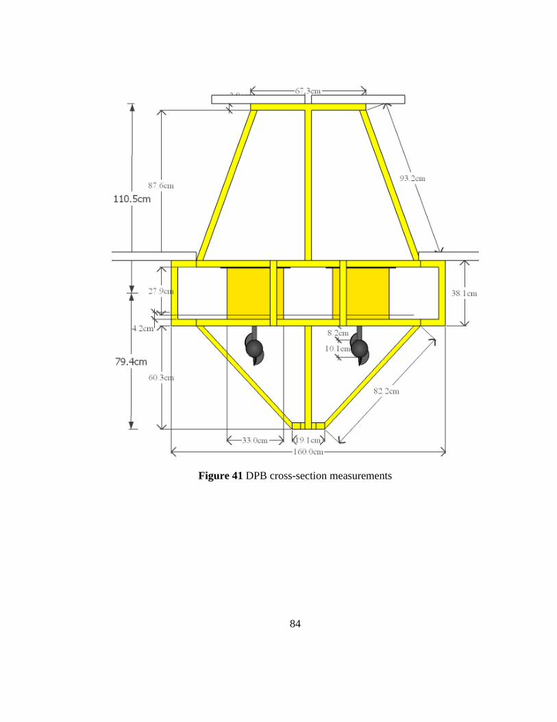
84
Figure 41 DPB cross-section measurements
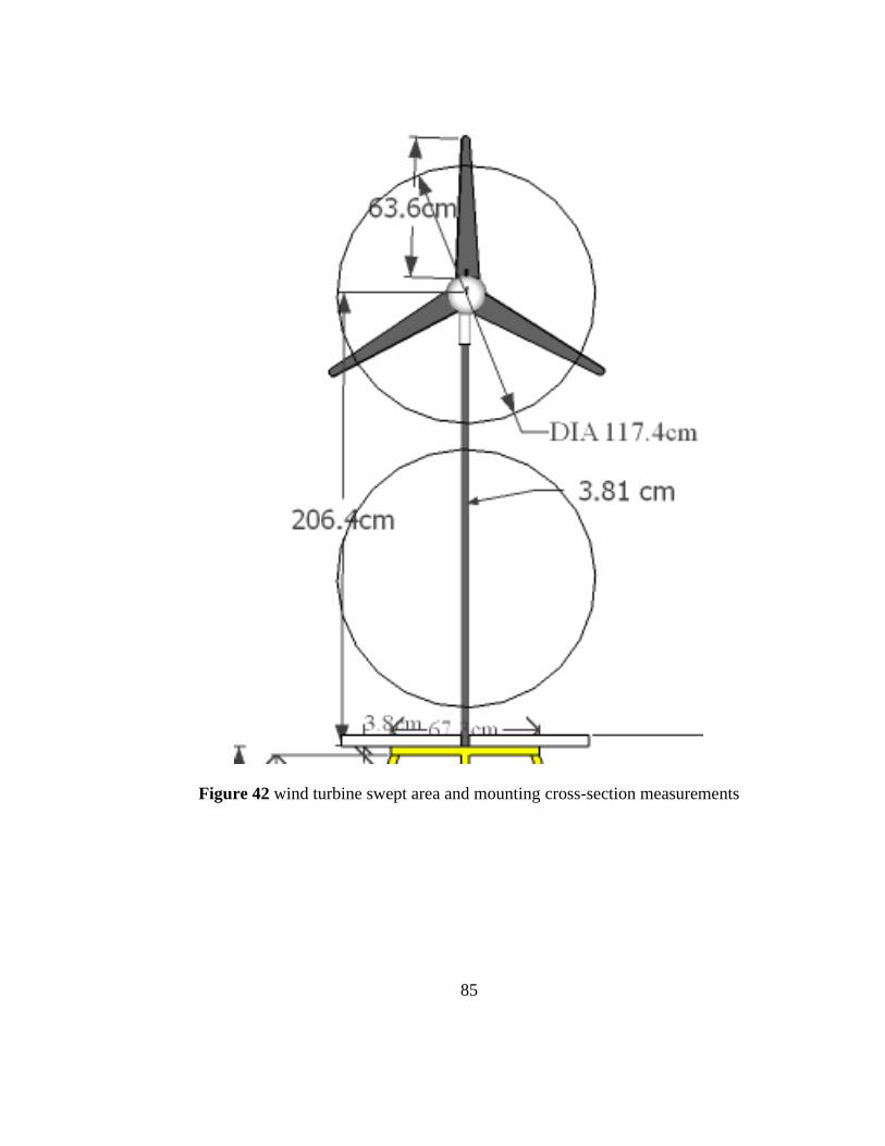
85
Figure 42 wind turbine swept area and mounting cross-section measurements
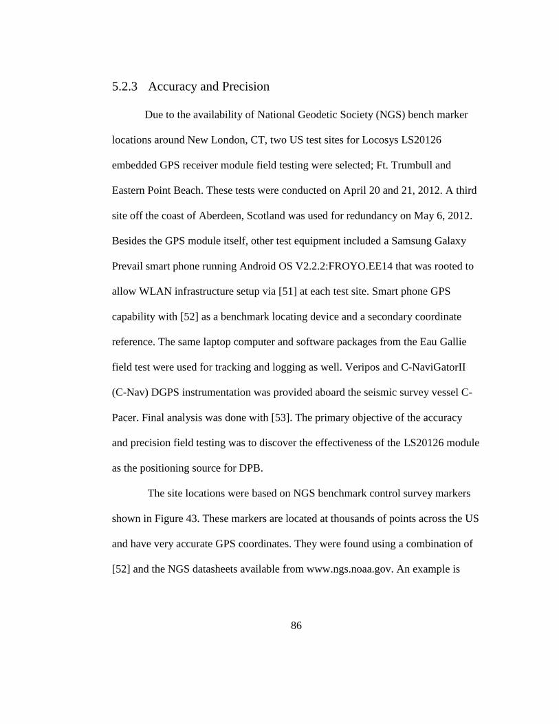
86
5.2.3 Accuracy and Precision
Due to the availability of National Geodetic Society (NGS) bench marker
locations around New London, CT, two US test sites for Locosys LS20126
embedded GPS receiver module field testing were selected; Ft. Trumbull and
Eastern Point Beach. These tests were conducted on April 20 and 21, 2012. A third
site off the coast of Aberdeen, Scotland was used for redundancy on May 6, 2012.
Besides the GPS module itself, other test equipment included a Samsung Galaxy
Prevail smart phone running Android OS V2.2.2:FROYO.EE14 that was rooted to
allow WLAN infrastructure setup via [51] at each test site. Smart phone GPS
capability with [52] as a benchmark locating device and a secondary coordinate
reference. The same laptop computer and software packages from the Eau Gallie
field test were used for tracking and logging as well. Veripos and C-NaviGatorII
(C-Nav) DGPS instrumentation was provided aboard the seismic survey vessel C-
Pacer. Final analysis was done with [53]. The primary objective of the accuracy
and precision field testing was to discover the effectiveness of the LS20126 module
as the positioning source for DPB.
The site locations were based on NGS benchmark control survey markers
shown in Figure 43. These markers are located at thousands of points across the US
and have very accurate GPS coordinates. They were found using a combination of
[52] and the NGS datasheets available from www.ngs.noaa.gov. An example is
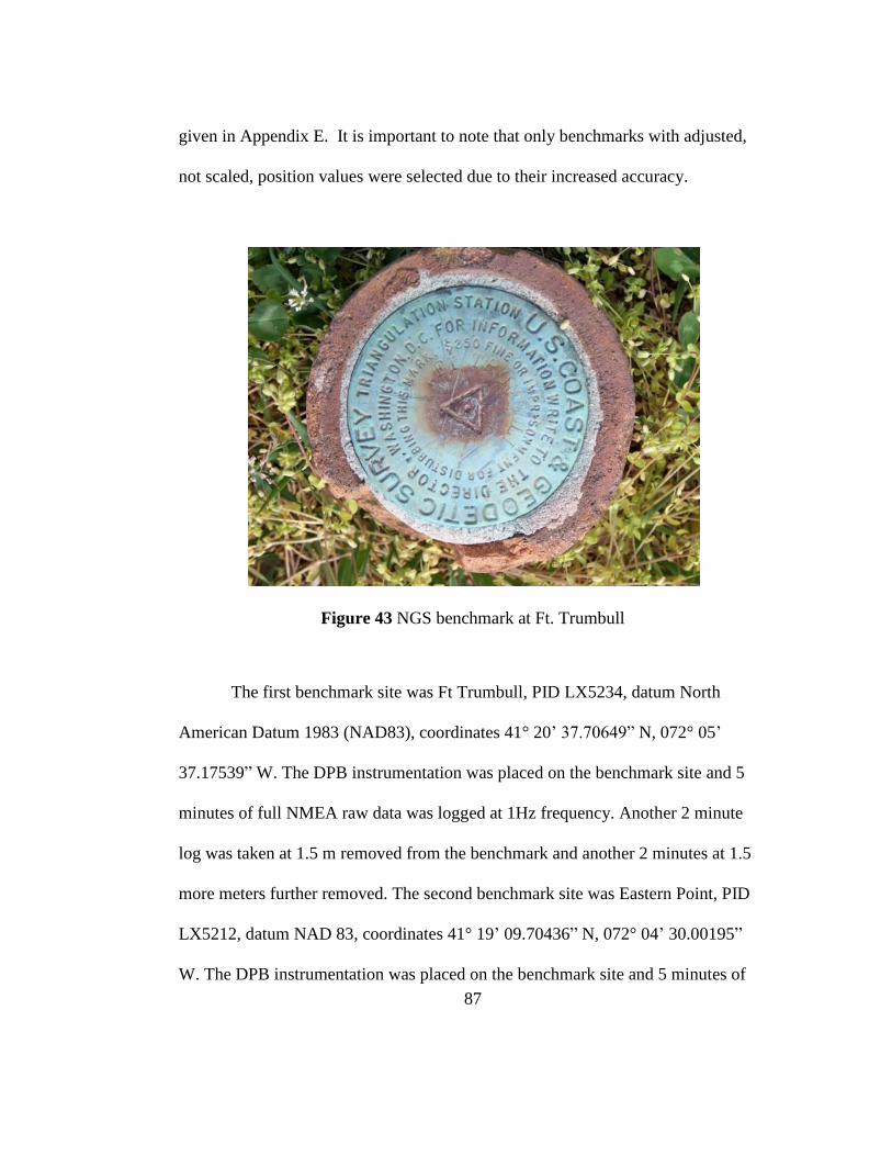
87
given in Appendix E. It is important to note that only benchmarks with adjusted,
not scaled, position values were selected due to their increased accuracy.
Figure 43 NGS benchmark at Ft. Trumbull
The first benchmark site was Ft Trumbull, PID LX5234, datum North
American Datum 1983 (NAD83), coordinates 41° 20’ 37.70649” N, 072° 05’
37.17539” W. The DPB instrumentation was placed on the benchmark site and 5
minutes of full NMEA raw data was logged at 1Hz frequency. Another 2 minute
log was taken at 1.5 m removed from the benchmark and another 2 minutes at 1.5
more meters further removed. The second benchmark site was Eastern Point, PID
LX5212, datum NAD 83, coordinates 41° 19’ 09.70436” N, 072° 04’ 30.00195”
W. The DPB instrumentation was placed on the benchmark site and 5 minutes of

88
full NMEA output string data were logged at 1Hz frequency. Another 5 minute log
was taken at 7.3 m North by Northeast from the Eastern Point marker. This
distance was selected to be greater than the 5 m accuracy of the LS20126 module
and based on the practical placement of the unit on a level surface away from the
original mark. A third test was conducted onboard the seismic node vessel C-Pacer
while outside the harbor in Aberdeen, Scotland, datum World Geodetic System
1984 (WGS 84), coordinates 057° 10’ 39.135” N, 002° 00’ 36.049” W using RTNu
corrected DGPS positioning data to ensure sub-meter accuracy. The DPB
instrumentation was placed next to the GPS antenna and 5 minutes of data
recorded. The unit was then moved to a pre-surveyed point on the vessel at a
known distance (11.6 m to port and 0.3 m forward) from the antenna and 5 minutes
of data was recorded. All $GPRMC strings were parsed for latitude and longitude
coordinates then plotted using [53].
The Ft. Trumbull benchmark was located on the top wall of the fort.
Luckily there were maintenance personnel on site that allowed access to the
benchmark for this test. Three positions within 3 m of each other were logged.
Unfortunately the log files were not taken separately so there was no way to tell
which position is which. Figure 44 shows all plotted coordinates from the Ft.
Trumbull field test.
89
Figure 44 Ft. Trumbull field test results
The Eastern Point Beach benchmark was the most easily accessible. It was
embedded into a large rock outcrop near the water in a public park. The benchmark
is shown as the diamond shaped mark in the lower left corner of Figure 45.
Lessons learned from the Ft. Trumbull test were the use of separate log files for
each position measurement. The plus shaped plots show position measurements
when the DPB instrumentation placed directly on the benchmark. Northing and
easting coordinates applied to the measurements during post analysis indicated that
the maximum outlier positions from the benchmark are within in a 15 m radius, an
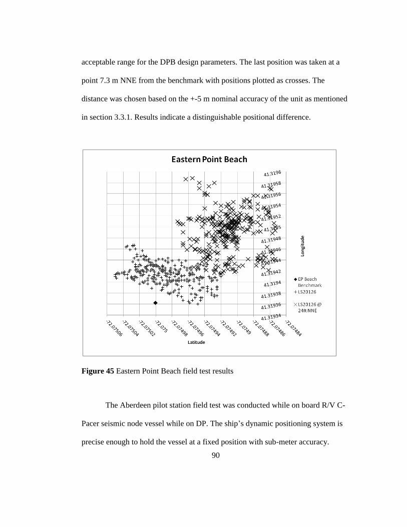
90
acceptable range for the DPB design parameters. The last position was taken at a
point 7.3 m NNE from the benchmark with positions plotted as crosses. The
distance was chosen based on the +-5 m nominal accuracy of the unit as mentioned
in section 3.3.1. Results indicate a distinguishable positional difference.
Figure 45 Eastern Point Beach field test results
The Aberdeen pilot station field test was conducted while on board R/V C-
Pacer seismic node vessel while on DP. The ship’s dynamic positioning system is
precise enough to hold the vessel at a fixed position with sub-meter accuracy.
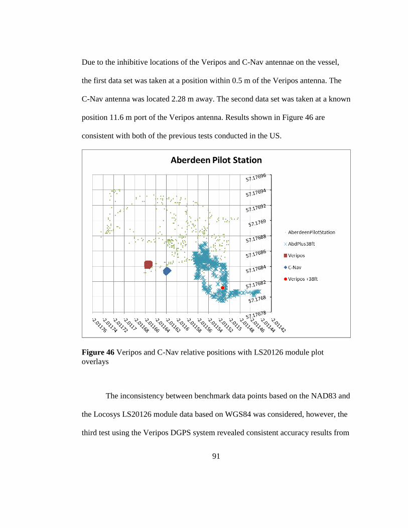
91
Due to the inhibitive locations of the Veripos and C-Nav antennae on the vessel,
the first data set was taken at a position within 0.5 m of the Veripos antenna. The
C-Nav antenna was located 2.28 m away. The second data set was taken at a known
position 11.6 m port of the Veripos antenna. Results shown in Figure 46 are
consistent with both of the previous tests conducted in the US.
Figure 46 Veripos and C-Nav relative positions with LS20126 module plot
overlays
The inconsistency between benchmark data points based on the NAD83 and
the Locosys LS20126 module data based on WGS84 was considered, however, the
third test using the Veripos DGPS system revealed consistent accuracy results from
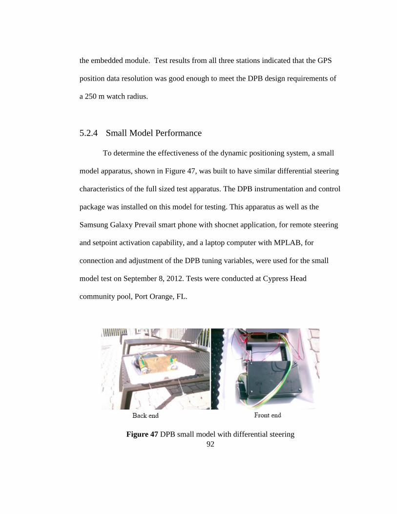
92
the embedded module. Test results from all three stations indicated that the GPS
position data resolution was good enough to meet the DPB design requirements of
a 250 m watch radius.
5.2.4 Small Model Performance
To determine the effectiveness of the dynamic positioning system, a small
model apparatus, shown in Figure 47, was built to have similar differential steering
characteristics of the full sized test apparatus. The DPB instrumentation and control
package was installed on this model for testing. This apparatus as well as the
Samsung Galaxy Prevail smart phone with shocnet application, for remote steering
and setpoint activation capability, and a laptop computer with MPLAB, for
connection and adjustment of the DPB tuning variables, were used for the small
model test on September 8, 2012. Tests were conducted at Cypress Head
community pool, Port Orange, FL.
Figure 47 DPB small model with differential steering
93
The objectives were to observe the maneuvering and controllability of the
model, test the station keeping capability of the DPB instrumentation and control
system, test the effectiveness of the zeroth order Kalman filter, and to test the
effectiveness of adjusting the tuning variables Q, R, associated with the filter, and
posfudge, brgfudge, turntimeCW, turntimeCCW, ahdtime, associated with the
allowable corrective ranges and duty cycles.
The first test was simply an observation of the maneuverability and
operation of the small craft by placing it the pool and connecting to it with shocnet.
The craft was then driven, remotely, through a series of left, right, and ahead full
maneuvers.
Once maneuverability was observed, the vessel was driven to a location
near the center of the pool. The set point then activated remotely and the craft
observed. The desired outcome was that the craft would remain stationary.
For positional correction, the tuning variables Q, process noise covariance,
and R, measurement noise covariance, are associated with the Kalman filter, and
refer to the certainties of the process model and measurements respectively. A high
value for R and low value for Q will not give too much weight to the measurements
and depend more heavily on the model while a low value for R and a high value for
Q will follow more closely to the measurements and give less dependency to the
model [19].
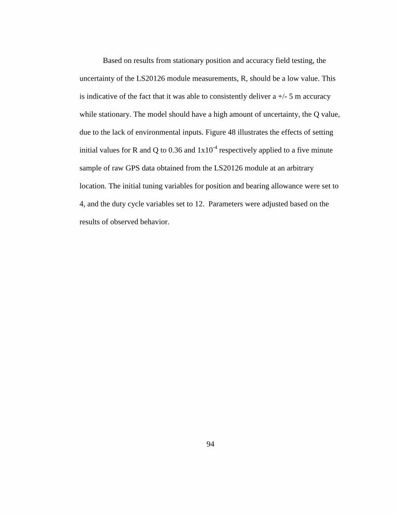
94
Based on results from stationary position and accuracy field testing, the
uncertainty of the LS20126 module measurements, R, should be a low value. This
is indicative of the fact that it was able to consistently deliver a +/- 5 m accuracy
while stationary. The model should have a high amount of uncertainty, the Q value,
due to the lack of environmental inputs. Figure 48 illustrates the effects of setting
initial values for R and Q to 0.36 and 1x10⁻⁴
respectively applied to a five minute
sample of raw GPS data obtained from the LS20126 module at an arbitrary
location. The initial tuning variables for position and bearing allowance were set to
4, and the duty cycle variables set to 12. Parameters were adjusted based on the
results of observed behavior.
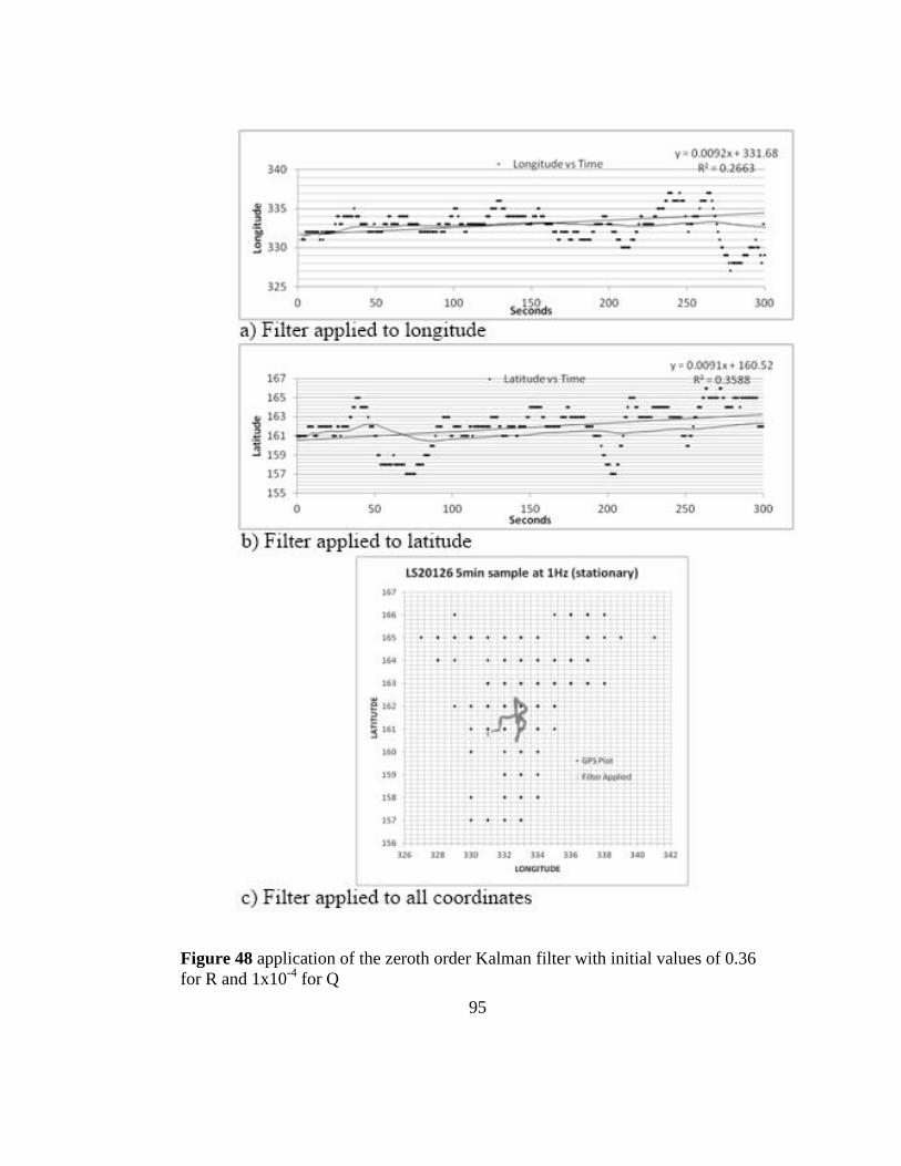
95
Figure 48 application of the zeroth order Kalman filter with initial values of 0.36
for R and 1x10⁻⁴
for Q
96
Observations of the initial maneuvering test revealed a left favored motion
during ahead full maneuvers. Ahead and CCW timing adjustment variables were
lowered to reduce the thruster on cycle those maneuvers. Figure 49 is satellite view
of the initial positioning test of DPB from [45]. Results indicate that the initially
applied filtering parameters were ineffective. Subsequent tests over a range of
tuning values yielded similar, disappointing, results.
Figure 49 from [45] a satellite image of small model test with the recorded path
superimposed
It was concluded that either the tuning parameters were ineffective as fixed
values and DPB would benefit from real-time, self-tuning, capability, or that the

97
relatively small dimensions of the pool were too restrictive for conclusive results of
the test. One key observation was that the influence of wind speed and direction
strongly dictated the positional offsets. This resulted in extreme changes of DPB
heading. The addition of an anemometer input to the system should greatly increase
the positional correction capability of DPB.

98
6. Conclusion and Further Development
The DPB system demonstrated the ability to mount a self-feathering,
horizontal axis wind turbine at a height of 3 m from the water line while
maintaining upright stability during maneuvering in wind speeds up to 2.5 m s-1
.
The originally conceived vertical axis wind turbine centered within the body of the
buoy, a radical concept which would alleviate wind attack angle concerns, was
discarded due to a lack of availability and size restrictions that would be imposed.
Among several other design considerations, such as structure, cost,
availability, and existing buoy designs, power requirements turned out to be
extremely prohibitive towards the practical use of a wind and solar hybrid
renewable energy system. While the optimal design configurations of a hybrid solar
and wind renewable energy system using a 10% propulsive duty cycle input to [54]
were able to attain a minimum capacity shortage of less than 1% at one Hawaiian
Islands location, all other simulated locations had results greater than 15%. A lack
battery storage capacity was also determined to contribute considerably to this
shortage. The addition of surface wave energy to the hybrid system was considered,
but after reviewing the results from [59] and an exhaustive internet search for off
the shelf linear generators it was concluded that a surface wave energy generator
system would be impractical at this time.
99
Using electric propulsion was concluded to be less effective than a direct
mechanical drive train due to the poor efficiencies associated with renewable
energy systems. An electric propulsion system also has a restrictive total output
which is independent of wind power, whereas a mechanical drive train would
provide an output that is simply proportional to and limited only by the wind speed.
An ideal, electro-mechanical, propulsion system would take advantage of heavy
wind or high solar irradiance conditions as well as provide back-up power and
propulsion during periods of low wind and poor insolation. A low cost dynamic
positioning system was deemed feasible, but overall limited with respect to the
selected microcontroller, lack of environmental sensing, precision positioning
module, and variable speed control.
6.1 A Better DPB Design
A better station keeping design, which has a propensity for station keeping,
should present the least amount of drift from position when affected by ocean and
wind currents, therefore, requiring the least amount of power input for corrections.
A similar buoy with rudder type steering and an electromechanical drive train could
be developed to use very little electrical power. Integration of inertial navigation
and dead reckoning would also provide reliability during periods of GPS blackout.
Also, Blackford acknowledges that the omni-directional nature of a vertical-axis
windmill should give a practical advantage in the application of rotary wind craft
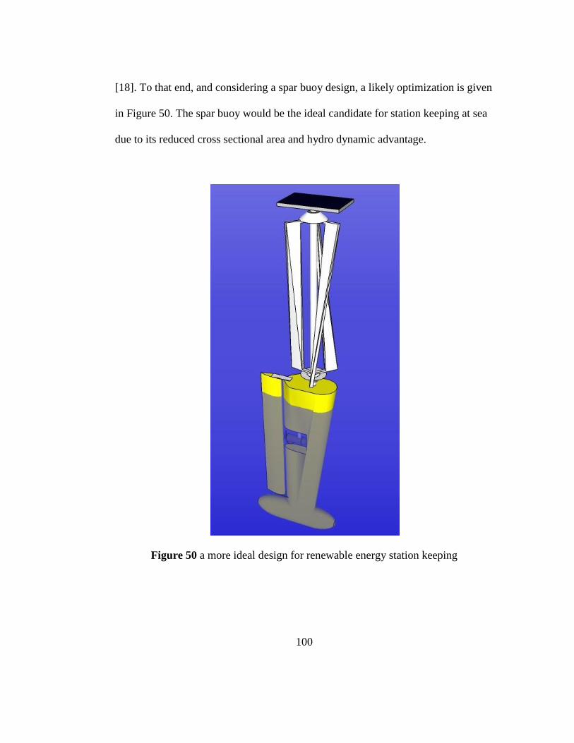
100
[18]. To that end, and considering a spar buoy design, a likely optimization is given
in Figure 50. The spar buoy would be the ideal candidate for station keeping at sea
due to its reduced cross sectional area and hydro dynamic advantage.
Figure 50 a more ideal design for renewable energy station keeping
101
6.2 Further Development
The sea anchor, or drag anchor, is another type of stationary positioning that
can be deployed from vessels floating on the surface. While anything submerged in
the water and tethered to a surface vessel can provide drag, most modern drag
anchors are shaped like upside down parachutes. They cannot hold a vessel
completely stationary, but a drag anchor could help mitigate the effects of wind
drift. Modern life boats use them to keep from drifting too far from the distress
position during search and rescue operations. An automated water drag system
addition, which could sense surface currents and determine a beneficial adjustment
angle, could provide extra drag as a counter force to wind currents in some cases.
The most highly recommended addition to the control system is an
anemometer for wind speed and direction data. A power sensor measurement,
motor speed control, accelerometer feedback, and current sensing are also valuable
inputs for the incorporation of a full blown DPS using a true extended Kalman
filter.
Solar tracking would provide increased performance of the renewable
energy system and could be accomplished by adjusting the mounting angle of the
panels along with heading correction based on photo sensing.
102
References
[1] Marshall, Amy K. A History of Buoys and Tenders. Web. 2011.
<http://www.uscg.mil/history/weblighthouses/h_buoys.asp>
[2] Moored Buoy Program. August 2006. Web. 2011.
<http://www.ndbc.noaa.gov/mooredbuoy.shtml>
[3] DARPA Solicitation Number BAA04-33. A -- Persistent Ocean
Surveillance (POS). July 30, 2004. Web. 2011. <https://www.fbo.gov/>
[4] DARPA Solicitation Number DARPASN08-45. STATION KEEPING
BUOY ENERGY HARVESTING/HARNESSING. July 31, 2008. Web. 2012.
<https://www.fbo.gov/>
[5] LOCOSYS Technology, Inc. Datasheet of stand-alone GPS smart antenna
module with magnetic sensor, LS20126. 2006.
[6] Microchip Technology, Inc. PIC18F47J13 FamilyData Sheet:28/44-Pin,
High-Performance Microcontrollers with nanoWatt XLP Technology.
2010.
[7] Burton T., Sharpe D., Jenkins N., and Bossanyi E. Wind Energy
Handbook. John Wiley & Sons, Ltd., New York. 2001.
[8] Gipe, Paul. Wind Power. The completely Revised and Expanded Edition.
Chelsea Green Publishing Company. White River Junction, VT. 2004.
[9] Daidola, John C., Basar, Nedret S., Reyling, Christopher J., Johnson,
Fontain M. and Walker, Richard T. Buoy Technology Survey Worldwide
103
Buoy Technology Survey. Rosenblatt & Son, Inc. New York, NY and
USCG R & D Center Avery Point, Groton, CT. 1991. Contract DTCG39-
89-C-E27E04. 2231 p. Available from: NTIS, Springfield, VA; CG-D-05-
92. Sponsored by Department of Transportation U. S. Coast Guard Office
of Engineering, Logistics and Development. Web. 2012.
<http://www.dtic.mil/>
[10] Bhattacharjee, Subir. ExxonMobil Development Company. Design and
Installation Challenges for Deepwater Mooring Systems. Web. 2011.
<http://www.vryhof.com/pdf/Exxonmobil.pdf>
[11] Sorensen, Bent. Renewable Energy: Its physics, engineering, use,
environmental impacts, economy and planning aspects. Second Edition.
Academic Press. San Diego, CA. 2000.
[12] Berteaux, H. O. Buoy Engineering. John Wiley & Sons. New York.1976.
[13] Outlaw, Adam S. Computerization of an Autonomous Mobile Buoy. M.S.
Thesis. Florida Institute of Technology. 2007.
[14] Marikle, Sean P. DYNAMIC POSITIONING AND MOTION MITIGATION
OF A SCALED SEA BASING PLATFORM. M.S. Thesis. Florida Atlantic
University. 2009.
[15] Introduction to Dynamic Positioning. Web. 2011. <www.imca-int.com/>
[16] Spera, Gabriel, and Storm, Steven R. A Brief History of Human
Navigation. Crosslink the Aerospace Corporation magazine of advances in
104
aerospace technology. Vol.3 No.2. p.51-53. Summer 2002. Web. 2012.
<http://www.aero.org/>
[17] Enge, Per, and Misra, Pratap. Scanning the Issue/Technology Special Issue
on Global Positioning System. Proceedings of the IEEE. Vol.87, No.1, p.3-
15, January 1999. Publisher Item Identifier S 0018-9219(99)00937-8. Web.
2012. <http://ieeexplore.ieee.org/stamp/stamp.jsp?arnumber=00736338>
[18] Blackford, B. L. "The Physics of a Push-me Pull-you Boat." American
Journal of Physics 46.10 (1978): 1004. Web. 2012. <http://ajp.aapt.org/>
[19] Welsh, Greg and Gary Bishop. An Introduction to the Kalman Filter.
University of Chapel Hill. North Carolina. 2006.
[20] Couch, Chris. "Compass Headings, Navigation and Equipment." Compass
Headings, Navigation and Equipment. Web. 2012.
<http://www.compassheadings.com/navigation.php>
[21] Juselis, Gregory J. Station Keeping Buoy System. The United States of
America as Represented by the Secretary of the Navy, Washington, D.C.,
assignee. Patent 5577942. 26 Nov. 1996. Web. 2012.
<http://www.google.com/patents/US5577942>
[22] Cardoza, Miguel A., William A. Adamez, Devin M. Tomlinson, Sarah A.
Benedict, and Mark H. Wolf. Water Drift Compensation Method and
Device. Patent 20090095208A1. 16 Apr. 2009. Web. 2012.
<http://www.google.com/patents/US20090095208>
105
[23] Pierce, Roger J. Stable Oceanic Station. Patent 3369516. 20 Feb. 1968.
Web. 2012. <http://www.google.com/patents/US3369516>
[24] Dane, Robert A., and Payne Killbourn. Unmanned Ocean Vehicle. Solar
Sailor Pty Ltd, assignee. Patent 7789723B2. 7 Sept. 2010. Web. 2012.
<http://www.google.com/patents/US7789723>
[25] Frizzell-Makowski, L. J., Shelsby, R. A., Mann, J. and Scheidt, D. "An
Autonomous Energy Harvesting Station-Keeping Vehicle for Persistent
Ocean Surveillance." Oceans 2011 Conference Publications. Web. 2012.
<ieeexplore.ieee.org/xpls/abs_all.jsp?arnumber=6106996>
[26] "Projects." SeaLandAire. SeaLandAireTechnologies, Inc. Web. 2012.
<http://sealandaire.com/projects/>
[27] DaSilva, S. J., Cleland, J., Chappell, S. G., and Graves, M. "Gatekeeper:
An Untethered, Persistent, Station-Keeping Gateway Buoy." Oceans 2009
Conference Publications. Web. 2011. < http://www.dtic.mil/>
[28] Curcio, J. A., Mcillivary, P. A., Fall, K., Maffei, A., Schwehr, K., Twiggs,
B., Kitts, C. and Ballou, P. “Self-Positioning Smart Buoys, The “Un-
Buoy” Solution: Logistic Considerations using Autonomous Surface Craft
Technology and Improved Communications Infrastructure.” Oceans 2006
Conference Publications. Web. 2011. < http://www.dtic.mil/>
106
[29] HobbyTronics. "Using Large Data Arrays in Microchip C18
Compiler." Using Large Data Arrays in Microchip C18 Compiler.
HobbyTronics, Ltd. Web. 2012. <http://www.hobbytronics.co.uk/>
[30] Worsley, Peter. "Rotary Sailing Homepage." Rotary Sailing Homepage.
Web. 2011. < http://sailwings.net/rotaryhome.html>
[31] Khaligh, Alireza, and Omer C. Onar. "Solar Energy Harvesting." Energy
Harvesting: Solar, Wind, and Ocean Energy Conversion Systems. Boca
Raton: CRC, 2010. 1-2.
[32] SRoeCo Solar. "SRoeCo Solar." Solar Panel Efficiency Comparison. Web.
2012. <http://sroeco.com/solar/most-efficient-solar-panels>
[33] "Which Solar Panel Type Is Best?" Energy Informative. Web. 2012.
<http://energyinformative.org/>
[34] DiPasquale, Roberta, Paul Przyborski, and Warren Wiscombe. "Measuring
Solar Insolation : Image of the Day." Measuring Solar Insolation : Image
of the Day. Surface Meteorology and Solar Energy Project, NASA Langley
Research Center, and the ISCCP Project. Web. 2012.
<http://earthobservatory.nasa.gov/IOTD/view.php?id=1355>
[35] Przymborski, Paul, and Warren Wiscombe. "NASA Earth Observatory :
Home." NASA Earth Observatory : Home. EOS Project Science Office
Located at NASA Goddard Space Flight Center. Web. 2012.
<http://earthobservatory.nasa.gov/>
107
[36] HOMER Energy. "History of HOMER and HOMER Energy." History of
HOMER Energy & HOMER Software for Hybrid Renewable & Distributed
Power Design Support. Web. 2012.
<http://www.homerenergy.com/history.html>.
[37] Bramer, Daniel, David Wojtowicz, and Steven Hall. "Global Wind
Patterns:wind Belts of the General Circulation." Global Wind
Patterns:wind Belts of the General Circulation. University of Illinois at
Urbana-Champaign, 1999. Web. 2012. <http://ww2010.atmos.uiuc.edu/ >
[38] Ragheb, M. Theory of Wind Machines, Betz Equation. CITE NetFiles.
University of Illinois at Urbana-Champaign, 2012. Web. 2012.
<https://netfiles.uiuc.edu/>
[39] Solar Systems USA, Inc. "Welcome to America's Trusted Source for
Buying Solar Panels Online." Solar Panels. Web. 2012.
<http://www.solarsystemsusa.net/>
[40] Southwest Windpower. "AIR Breeze | Southwest Windpower." AIR Breeze
| Southwest Windpower. Web. 2012.
<http://www.windenergy.com/products/air/air-breeze>
[41] Buchman, Isidor. "Welcome To Battery University." Basic to Advanced
Battery Information from Battery University. Cadex Electronics, Inc. Web.
2012. <http://www.batteryuniversity.com/>
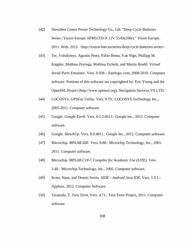
108
[42] Shenzhen Center Power Technology Co., Ltd. "Deep Cycle Batteries
Series | Vision Europe: 6FM55TD-X 12V 55Ah(20hr)." Vision Europe.
2011. Web. 2012. <http://vision-batt.eu/series/deep-cycle-batteries-series>
[43] Ter, Volodymyr, Agustin Perez, Fabio Bema, Yan Nign, Phillipp M.
Kappler, Mathieu Peyrega, Mathieu Fichefe, and Martin Hradil. Virtual
Serial Ports Emulator. Vers. 0.938. : Eterlogic.com, 2008-2010. Computer
software. Portions of this software are copyrighted by: Eric Young and the
OpenSSL Project (http://www.openssl.org), Navigation Services VS LTD.
[44] LOCOSYS. GPSFox Utility. Vers. 0.79.: LOCOSYS Technology Inc.,
2005-2011. Computer software.
[45] Google. Google Earth. Vers. 6.2.2.6613.: Google Inc., 2012. Computer
software.
[46] Google. SketchUp. Vers. 8.0.4811.: Google Inc., 2012. Computer software.
[47] Microchip. MPLAB IDE. Vers. 8.80.: Microchip Technology, Inc., 2001-
2011. Computer software.
[48] Microchip. MPLAB C18 C Compiler for Academic Use (LITE). Vers.
3.40.: Microchip Technology, Inc., 2005. Computer software.
[49] Kratz, Hans, and Dennis Strein. AIDE - Android Java IDE. Vers. 1.0.1.:
Appfour, 2012. Computer Software.
[50] Teranishi, T. Tera Term. Vers. 4.71.: Tera Term Project, 2011. Computer
software.
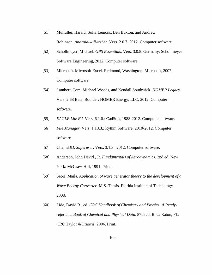
109
[51] Mulluller, Harald, Sofia Lemons, Ben Buxton, and Andrew
Robinson. Android-wifi-tether. Vers. 2.0.7. 2012. Computer software.
[52] Schollmeyer, Michael. GPS Essentials. Vers. 3.0.8. Germany: Schollmeyer
Software Engineering, 2012. Computer software.
[53] Microsoft. Microsoft Excel. Redmond, Washington: Microsoft, 2007.
Computer software.
[54] Lambert, Tom, Michael Woods, and Kendall Southwick. HOMER Legacy.
Vers. 2.68 Beta. Boulder: HOMER Energy, LLC, 2012. Computer
software.
[55] EAGLE Lite Ed. Vers. 6.1.0.: CadSoft, 1988-2012. Computer software.
[56] File Manager. Vers. 1.13.3.: Rythm Software, 2010-2012. Computer
software.
[57] ChainsDD. Superuser. Vers. 3.1.3., 2012. Computer software.
[58] Anderson, John David., Jr. Fundamentals of Aerodynamics. 2nd ed. New
York: McGraw-Hill, 1991. Print.
[59] Sepri, Maila. Application of wave generator theory to the development of a
Wave Energy Converter. M.S. Thesis. Florida Institute of Technology.
2008.
[60] Lide, David R., ed. CRC Handbook of Chemistry and Physics: A Ready-
reference Book of Chemical and Physical Data. 87th ed. Boca Raton, FL:
CRC Taylor & Francis, 2006. Print.
110
[61] Savage, Marshall T. The Millennial Project: Colonizing the Galaxy in
Eight Easy Steps. New York: Little, Brown and, 1994. Print.
[62] Wood, S., Reese, M., and Pfeiffer, Z. "An Autonomous Self-Mooring
Vehicle for Littoral & Coastal Observations." Oceans 2007 Conference
Publications. Web. 2012. < http://ieeexplore.ieee.org/>
[63] Stackhouse, Paul W., Jr., and John M. Kusterer. "Surface Meteorology and
Solar Energy." Surface Meteorology and Solar Energy. NASA Langley
ASDC User Services, 4 Sept. 2012. Web. 2012.
<http://eosweb.larc.nasa.gov/sse/>
[64] Emery, Kenith. "Solar Spectral Irradiance: Air Mass 1.5." Solar Spectral
Irradiance: Air Mass 1.5. U.S. Department of Energy by the Alliance for
Sustainable Energy, LLC, 2009. Web. 2012.
<http://rredc.nrel.gov/solar/spectra/am1.5/>.
[65] NovAtel. "GPS Position Accuracy Measures." APN-029 Rev 1. Novatel
Positioning Leaders, 2003. Web. 2012. <http://webone.novatel.ca>.
111
Appendix A (Third Party Software Packages)
Figure 51 from [44] LS20126 module monitoring software including
accelerometer output
Figure 52 from [43] used to redirect and split TCP/IP port connections to virtual
serial port
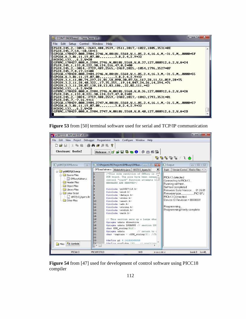
112
Figure 53 from [50] terminal software used for serial and TCP/IP communication
Figure 54 from [47] used for development of control software using PICC18
compiler
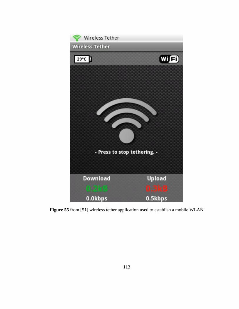
113
Figure 55 from [51] wireless tether application used to establish a mobile WLAN

114
Figure 56 from [49] used for mobile application development
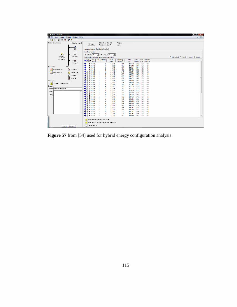
115
Figure 57 from [54] used for hybrid energy configuration analysis

116
Appendix B (PIC C-18 Control Code)
C:\Projects\PICProjects\DPBuoy\DPBuoyKalman.c
/*This code rendition of DPBuoy is further developed than DPBuoy_GPS_27j12PCB.c
as is was developed for the PCB board. The pins have been remapped for the pc
board. The get_bearing is completed and the control "track" function attempts
to use the filter to get positions. THE LCD FUNCTIONS AND DISPLAY MESSAGES ARE
REMOVED*/
#include <p18f27j13.h>
#include <xlcd.h>
#include <delays.h>
#include <stdio.h>
#include <usart.h>
#include <adc.h>
#include <string.h>
#include <stdlib.h>
#include <math.h>
// this section sets up a large character array by combining 3 banks of 256
bytes. Be sure to use
"18f27j13lrgarry.lkr" files.
#pragma udata directive
#pragma udata LRGARRY // section LRGARRY
char GPS_string[512];
#pragma udata // return to default section
char *capture = &GPS_string[0]; //Use a pointer to access the values in the
large array
#define pi 3.14159265359
#define posfudge 150 // positional offset allowance
#define brgfudge 10 // bearing offset allowance
#define turntimeCW 12 // how long the thrusters stay on for turning
Clockwise corrections
#define turntimeCCW 4 // how long the thrusters stay on for turning
Counterclockwise corrections
#define ahdtime 12 // how long the thrusters stay on for ahead full
corrections
#define R 0.36 //(R-measurement noise covariance) represents the
uncertainty in the measurement
#define Q 0.0001 //(Q-Process noise covariance) represents the
uncertainty in the process model
// A tight filter: large R and small Q will not give too much weight to the
measurements
// A relaxed filter: small R and large Q will follow more closely to the
measurements
//Fucntion Prototypes.............................................
int get_heading(void);
void get_bearing(void);
void get_position(void);
void kalman_filter(void);
void track(void);
void move_far(void);
void manual_control(void);
//Global Variables.......................................
char PLSR_parse[]="PLSR,245,1",GPRMC_parse[]="GPRMC",delim1[]="$*",delim2[]=
",.",PLSR_parsed[80],GPRMC_parsed[80];
char NSmk='X',*NSind,EWmk='X',*EWind;
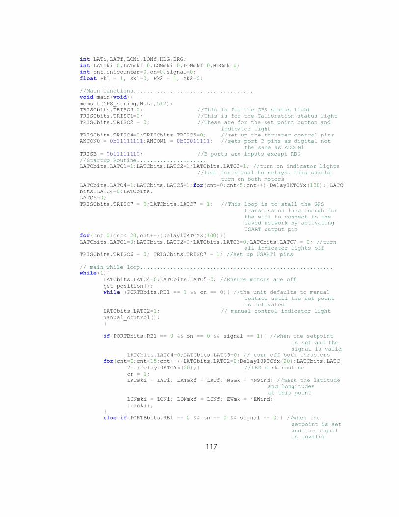
117
int LATi,LATf,LONi,LONf,HDG,BRG;
int LATmki=0,LATmkf=0,LONmki=0,LONmkf=0,HDGmk=0;
int cnt,inicounter=0,on=0,signal=0;
float Pk1 = 1, Xk1=0, Pk2 = 1, Xk2=0;
//Main functions....................................
void main(void){
memset(GPS_string,NULL,512);
TRISCbits.TRISC3=0; //This is for the GPS status light
TRISCbits.TRISC1=0; //This is for the Calibration status light
TRISCbits.TRISC2 = 0; //These are for the set point button and
indicator light
TRISCbits.TRISC4=0;TRISCbits.TRISC5=0; //set up the thruster control pins
ANCON0 = 0b11111111;ANCON1 = 0b00011111; //sets port B pins as digital not
the same as ADCON1
TRISB = 0b11111110; //B ports are inputs except RB0
//Startup Routine.....................
LATCbits.LATC1=1;LATCbits.LATC2=1;LATCbits.LATC3=1; //turn on indicator lights
//test for signal to relays. this should
turn on both motors
LATCbits.LATC4=1;LATCbits.LATC5=1;for(cnt=0;cnt<5;cnt++){Delay1KTCYx(100);}LATC
bits.LATC4=0;LATCbits.
LATC5=0;
TRISCbits.TRISC7 = 0;LATCbits.LATC7 = 1; //This loop is to stall the GPS
transmission long enough for
the wifi to connect to the
saved network by activating
USART output pin
for(cnt=0;cnt<=20;cnt++){Delay10KTCYx(100);}
LATCbits.LATC1=0;LATCbits.LATC2=0;LATCbits.LATC3=0;LATCbits.LATC7 = 0; //turn
all indicator lights off
TRISCbits.TRISC6 = 0; TRISCbits.TRISC7 = 1; //set up USART1 pins
// main while loop..........................................................
while(1){
LATCbits.LATC4=0;LATCbits.LATC5=0; //Ensure motors are off
get_position();
while (PORTBbits.RB1 == 1 && on == 0){ //the unit defaults to manual
control until the set point
is activated
LATCbits.LATC2=1; // manual control indicator light
manual_control();
}
if(PORTBbits.RB1 == 0 && on == 0 && signal == 1){ //when the setpoint
is set and the
signal is valid
LATCbits.LATC4=0;LATCbits.LATC5=0; // turn off both thrusters
for(cnt=0;cnt<15;cnt++){LATCbits.LATC2=0;Delay10KTCYx(20);LATCbits.LATC
2=1;Delay10KTCYx(20);} //LED mark routine
on = 1;
LATmki = LATi; LATmkf = LATf; NSmk = *NSind; //mark the latitude
and longitudes
at this point
LONmki = LONi; LONmkf = LONf; EWmk = *EWind;
track();
}
else if(PORTBbits.RB1 == 0 && on == 0 && signal == 0){ //when the
setpoint is set
and the signal
is invalid
118
printf("Can't track, no valid signal");
Nop();
}
}
}
//End of main.................................................................
void get_position(void){
long UTCi;
int UTCf;
int SOGi,SOGf,COGi,COGf,DATE,vlength,nmhldr;
float flthldr;
char *gps,*name,*UTC,*valid,*mode,*plchldr;
memset(GPS_string,NULL,512);
TRISCbits.TRISC3=0; //This is for the GPS status light
Open1USART(USART_TX_INT_OFF & USART_RX_INT_ON & USART_ASYNCH_MODE &
USART_EIGHT_BIT & USART_CONT_RX
& USART_BRGH_HIGH,129);
while(!DataRdy1USART());
for(cnt=0;cnt<=511;cnt++){
while(!DataRdy1USART());
capture[cnt]=Read1USART();
}cnt = 0;
sprintf(GPRMC_parsed,"%s",strtok(strstr(capture,GPRMC_parse),delim1));
vlength = strlen(GPRMC_parsed);
// Get the sub-parsed Data Strings............................
name = strtok(GPRMC_parsed,delim2);
UTCi = atol(strtok(NULL,delim2));UTCf = atoi(strtok(NULL,delim2));
valid = strtok(NULL,delim2);
if (*valid == 'V'){
signal = 0;
LATi=0;LATf=0;LONi=0;LONf=0;*NSind = 'X';*EWind = 'X';
HDG = get_heading();
LATCbits.LATC3 = 1;Delay1KTCYx(75);LATCbits.LATC3 = 0;
on = 0; //break from while loop in tracking
function
inicounter = 0; //this indicates that new apriori
data is required for the
kalman filter
printf("Signal=%d HDG: %d inicounter: %d\n\r",signal,HDG,inicounter);
}
else if (*valid == 'A'&& vlength>=50){
signal = 1;
//latitude, longitude CONVERSION to decimal
/* nmhldr =
atoi(strtok(NULL,delim2));flthldr=atof(strtok(NULL,delim2))/10000;
LATi = nmhldr/100; LATf =
(int)((((fmod(nmhldr,100)/60))+(flthldr/60))*10000);
NSind = strtok(NULL,delim2);
nmhldr =
atoi(strtok(NULL,delim2));flthldr=atof(strtok(NULL,delim2))/10000;
LONi = nmhldr/100; LONf =
(int)((((fmod(nmhldr,100)/60))+(flthldr/60))*10000);
EWind = strtok(NULL,delim2);*/
/* //latitude, longitude NO CONVERSION to decimal
LATi = atoi(strtok(NULL,delim2));LATf = atoi(strtok(NULL,delim2));
NSind = strtok(NULL,delim2);
LONi = atoi(strtok(NULL,delim2));LONf = atoi(strtok(NULL,delim2));
119
EWind = strtok(NULL,delim2); */
//degmin sec Lati:####dm Latf:##sec format
LATi = atoi(strtok(NULL,delim2));LATf = .06 *
(atoi(strtok(NULL,delim2)));
NSind = strtok(NULL,delim2);
LONi = atoi(strtok(NULL,delim2));LONf = .06 *
(atoi(strtok(NULL,delim2)));
EWind = strtok(NULL,delim2);
SOGi = atoi(strtok(NULL,delim2));SOGf = atoi(strtok(NULL,delim2));
COGi = atoi(strtok(NULL,delim2));COGf = atoi(strtok(NULL,delim2));
DATE = atoi(strtok(NULL,delim2));
plchldr = strtok(NULL,delim2);plchldr = strtok(NULL,delim2);
mode = strtok(NULL,delim2);
LATCbits.LATC3 = 1; //GPS status LED is on
HDG = COGi;
if (inicounter == 0){Xk1=LATf;Xk2=LONf;inicounter++;}
//this is gives the kalman filter apriori data
every time a signal is re-acquired
else{inicounter=1;}
//this stops the inicounter from counting
until signal islost in which case the
inicounter will be zero
printf("\n\rLATf: %d LONf:%d Signal:%d
inicounter:%d\n\r",LATf,LONf,signal,inicounter);
kalman_filter();
}
else{LATCbits.LATC3 = 1;Delay10KTCYx(75);LATCbits.LATC3 = 0;}
}
void kalman_filter(void){
float Pkminus1,Kk1,Zk1; //Covariance, updated covariance, Prediction, Kalman
error, measured state Latitude
float Pkminus2,Kk2,Zk2; //Covariance, updated covariance, Prediction, Kalman
error, measured state Longitude
Open1USART(USART_TX_INT_OFF & USART_RX_INT_ON & USART_ASYNCH_MODE &
USART_EIGHT_BIT & USART_CONT_RX & USART_BRGH_HIGH,129);
//filter latitude
Zk1 = LATf; //get the current measurement
Pkminus1 = (Pk1+Q);
Kk1 = Pkminus1/(Pkminus1+R);
Xk1 = Xk1 + (Kk1*(Zk1-Xk1));
Pk1 = (1-Kk1)*Pkminus1;
//filter longitude
Zk2 = LONf;
Pkminus2 = (Pk2+Q);
Kk2 = Pkminus2/(Pkminus2+R);
Xk2 = Xk2 + (Kk2*(Zk2-Xk2));
Pk2 = (1-Kk2)*Pkminus2;
LATf = (int)(Xk1*10);
LONf = (int)(Xk2*10);
printf("Filtered Lat:%d Filtered Lon:%d\n\r",LATf,LONf);
}
int get_heading (void){
char *name;
int ident,dir,field,accX,accY,accZ,tptrC,tptrF,mtmd,cal,autocal;
memset(GPS_string,NULL,512);
120
Open1USART(USART_TX_INT_OFF & USART_RX_INT_ON & USART_ASYNCH_MODE &
USART_EIGHT_BIT & USART_CONT_RX & USART_BRGH_HIGH,129);
while(!DataRdy1USART());
for(cnt=0;cnt<=511;cnt++){
while(!DataRdy1USART());
capture[cnt]=Read1USART();
}cnt = 0;
sprintf(PLSR_parsed,"%s",strtok(strstr(capture,PLSR_parse),delim1));
if (strlen(PLSR_parsed) >= 10){
name = strtok(PLSR_parsed,delim2);
ident = atoi(strtok(NULL,delim2));ident = atoi(strtok(NULL,delim2));
dir = atoi(strtok(NULL,delim2));
autocal = atoi(strtok(NULL,delim2));
field = atoi(strtok(NULL,delim2));
accX = atoi(strtok(NULL,delim2));accY = atoi(strtok(NULL,delim2));accZ
= atoi(strtok(NULL,delim2));
tptrC = atoi(strtok(NULL,delim2));tptrF = tptrC*9/5+32;
mtmd = atoi(strtok(NULL,delim2));
cal = atoi(strtok(NULL,delim2));
// Print values to buffers if the string is identified as PLSR,245,1 vice 245,2
or 245,7
if (autocal == 0){
LATCbits.LATC1 = 1;Delay1KTCYx(75);LATCbits.LATC1 = 0;}
else if (autocal>0 && autocal <7){
LATCbits.LATC1 = 1;Delay1KTCYx(75);LATCbits.LATC1 = 0;}
else if (autocal == 7){
LATCbits.LATC1 = 1;}
else{Nop();}
return dir;
}
else {Nop();}
}
void get_bearing(void){
int xLATi,xLATf,yLONi,yLONf,offset,add;
xLATi = LATmki - LATi;xLATf = LATmkf - LATf; //discover x distance from
setpoint
yLONi = LONmki - LONi;yLONf = LONmkf - LONf; //discover y distance from
setpoint
printf("xLATf: %d yLONf: %d\n\r",xLATf,yLONf);
if (xLATi != 0 || yLONi != 0){move_far();}
else if (xLATf >= posfudge && yLONf == 0) {BRG = 180;return;//N
else if (xLATf >= posfudge && yLONf >= posfudge) {add =
180;xLATf=fabs(xLATf);yLONf=fabs(yLONf);} //SW Q3
else if (xLATf == 0 && yLONf >= posfudge) {BRG = 270;return;}//E
else if (xLATf <= -posfudge && yLONf >= posfudge) {add =
270;xLATf=fabs(xLATf);yLONf=fabs(yLONf);} //NW Q4
else if (xLATf <= -posfudge && yLONf == 0) {BRG = 360;return;} //S
else if (xLATf <= -posfudge && yLONf <= -posfudge){add =
0;xLATf=fabs(xLATf);yLONf=fabs(yLONf);} //NE Q1
else if (xLATf == 0 && yLONf <= -posfudge){BRG = 90;return;}//W
else if (xLATf >= posfudge && yLONf <= -posfudge){add =
90;xLATf=fabs(xLATf);yLONf=fabs(yLONf);} //SE Q2
else {Nop();return;} //NA
offset = (atan2(yLONf,xLATf))* (180/pi); //calculate offset to degrees
BRG = add+offset;
printf("BRG: %d OFFST: %d add: %d\n\r",BRG, offset,add);
}
void track(void){
121
while (on = 1){
if(PORTBbits.RB1 == 1 && on == 1){ //if the button has already been
pressed (on = 1) and it gets
pressed again,set on to off
(on == 0)
LATmki=0;LATmkf=0;LONmki=0;LONmkf=0;NSmk = 'X';EWmk='X';HDGmk=0;
for
(cnt=0;cnt<5;cnt++){LATCbits.LATC2=0;Delay10KTCYx(100);LATCbits.LATC2=1
;Delay10KTCYx(100);}
LATCbits.LATC2=0; //unmark setpiont routine
on = 0;Close1USART();
break;}
else{
get_position();
if (signal == 0){break;}
get_bearing();
}
//Set up and make comparisons with and pulse the output voltage.
if (HDG<(BRG-brgfudge) || HDG>(BRG+brgfudge) ){ //if heading is not within +/-
brgfudge deg and bearing is
0-180deg turn clockwise by
activating port thruster
if(BRG <180){
LATCbits.LATC4=1;for
(cnt=0;cnt<turntimeCW;cnt++){Delay1KTCYx(100);}LATCbits.LATC4=0;
}
else if ( BRG >=180){ //if heading is not within +/- brgfudge deg and
bearing is 180-360 deg turn counter
clockwise by activating starboard thruster
LATCbits.LATC5=1;
for
(cnt=0;cnt<turntimeCCW;cnt++){Delay1KTCYx(100);}LATCbits.LATC5=0;
}
}
else if (HDG>(BRG-brgfudge) || HDG<(BRG+brgfudge) ){ //activate both
thrusters to
move forward
this is a
longer thrust
move than the
directional
moves
for
(cnt=0;cnt<ahdtime;cnt++){LATCbits.LATC4=1;LATCbits.LATC5=1;Delay1KTCYx
(100);LATCbits.LATC4=0;LATCbits.LATC5=0;}
}
else{Nop();}
}
}
void move_far(void){
// this function is to be written at a later date
}
void manual_control(void){
LATCbits.LATC2=1;Delay10KTCYx(100); //incdicator light
if (PORTBbits.RB3 == 1 && PORTBbits.RB2 == 0){
LATCbits.LATC4=1; //turn on port thruster
LATCbits.LATC5=0; //turn off starboard thruster
}
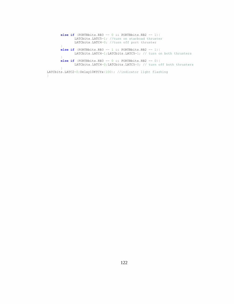
122
else if (PORTBbits.RB3 == 0 && PORTBbits.RB2 == 1){
LATCbits.LATC5=1; //turn on starboad thruster
LATCbits.LATC4=0; //turn off port thruster
}
else if (PORTBbits.RB3 == 1 && PORTBbits.RB2 == 1){
LATCbits.LATC4=1;LATCbits.LATC5=1; // turn on both thrusters
}
else if (PORTBbits.RB3 == 0 && PORTBbits.RB2 == 0){
LATCbits.LATC4=0;LATCbits.LATC5=0; // turn off both thrusters
}
LATCbits.LATC2=0;Delay10KTCYx(100); //indicator light flashing
}

123
Appendix C (18f27j13_lrgarry.lkr)
#DEFINE _CODEEND _DEBUGCODESTART - 1
#DEFINE _CEND _CODEEND + _DEBUGCODELEN
#DEFINE _DATAEND _DEBUGDATASTART - 1
#DEFINE _DEND _DATAEND + _DEBUGDATALEN
LIBPATH .
#IFDEF _CRUNTIME
#IFDEF _EXTENDEDMODE
FILES c018i_e.o
FILES clib_e.lib
FILES p18f27j13_e.lib
#ELSE
FILES c018i.o
FILES clib.lib
FILES p18f27j13.lib
#FI
#FI
#IFDEF _DEBUGCODESTART
CODEPAGE NAME=page START=0x0 END=_CODEEND
CODEPAGE NAME=debug START=_DEBUGCODESTART END=_CEND PROTECTED
#ELSE
CODEPAGE NAME=page START=0x0 END=0x1FFF7
#FI
CODEPAGE NAME=config START=0x1FFF8 END=0x1FFFF PROTECTED
CODEPAGE NAME=devid START=0x3FFFFE END=0x3FFFFF PROTECTED
#IFDEF _EXTENDEDMODE
DATABANK NAME=gpre START=0x0 END=0x5F
#ELSE
ACCESSBANK NAME=accessram START=0x0 END=0x5F
#FI
DATABANK NAME=gpr0 START=0x60 END=0xFF
DATABANK NAME=lrgarry START=0x100 END=0x2FF PROTECTED
DATABANK NAME=gpr3 START=0x300 END=0x3FF
DATABANK NAME=gpr4 START=0x400 END=0x4FF
DATABANK NAME=gpr5 START=0x500 END=0x5FF
DATABANK NAME=gpr6 START=0x600 END=0x6FF
DATABANK NAME=gpr7 START=0x700 END=0x7FF
DATABANK NAME=gpr8 START=0x800 END=0x8FF
DATABANK NAME=gpr9 START=0x900 END=0x9FF
DATABANK NAME=gpr10 START=0xA00 END=0xAFF
DATABANK NAME=gpr11 START=0xB00 END=0xBFF
DATABANK NAME=gpr12 START=0xC00 END=0xCFF
#IFDEF _DEBUGDATASTART
DATABANK NAME=gpr13 START=0xD00 END=_DATAEND
DATABANK NAME=dbgspr START=_DEBUGDATASTART END=_DEND PROTECTED
#ELSE //no debug
DATABANK NAME=gpr13 START=0xD00 END=0xDFF
#FI
DATABANK NAME=gpr14 START=0xE00 END=0xEAF
DATABANK NAME=sfr14 START=0xEB0 END=0xEFF PROTECTED
DATABANK NAME=sfr15 START=0xF00 END=0xF5F PROTECTED
ACCESSBANK NAME=accesssfr START=0xF60 END=0xFFF PROTECTED
#IFDEF _CRUNTIME
SECTION NAME=CONFIG ROM=config
SECTION NAME=LRGARRY RAM=lrgarry
#IFDEF _DEBUGDATASTART
STACK SIZE=0x100 RAM=gpr12
#ELSE
STACK SIZE=0x100 RAM=gpr13
#FI
#FI
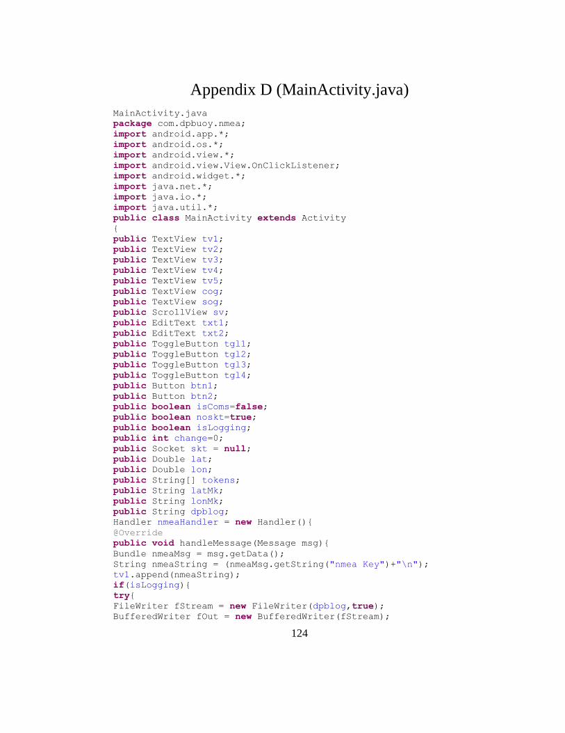
124
Appendix D (MainActivity.java)
MainActivity.java
package com.dpbuoy.nmea;
import android.app.*;
import android.os.*;
import android.view.*;
import android.view.View.OnClickListener;
import android.widget.*;
import java.net.*;
import java.io.*;
import java.util.*;
public class MainActivity extends Activity
{
public TextView tv1;
public TextView tv2;
public TextView tv3;
public TextView tv4;
public TextView tv5;
public TextView cog;
public TextView sog;
public ScrollView sv;
public EditText txt1;
public EditText txt2;
public ToggleButton tgl1;
public ToggleButton tgl2;
public ToggleButton tgl3;
public ToggleButton tgl4;
public Button btn1;
public Button btn2;
public boolean isComs=false;
public boolean noskt=true;
public boolean isLogging;
public int change=0;
public Socket skt = null;
public Double lat;
public Double lon;
public String[] tokens;
public String latMk;
public String lonMk;
public String dpblog;
Handler nmeaHandler = new Handler(){
@Override
public void handleMessage(Message msg){
Bundle nmeaMsg = msg.getData();
String nmeaString = (nmeaMsg.getString("nmea Key")+"\n");
tv1.append(nmeaString);
if(isLogging){
try{
FileWriter fStream = new FileWriter(dpblog,true);
BufferedWriter fOut = new BufferedWriter(fStream);
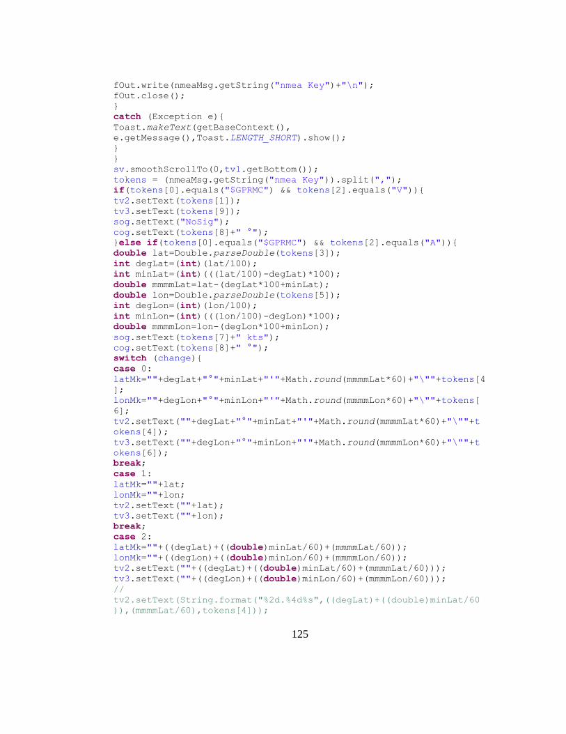
125
fOut.write(nmeaMsg.getString("nmea Key")+"\n");
fOut.close();
}
catch (Exception e){
Toast.makeText(getBaseContext(),
e.getMessage(),Toast.LENGTH_SHORT).show();
}
}
sv.smoothScrollTo(0,tv1.getBottom());
tokens = (nmeaMsg.getString("nmea Key")).split(",");
if(tokens[0].equals("$GPRMC") && tokens[2].equals("V")){
tv2.setText(tokens[1]);
tv3.setText(tokens[9]);
sog.setText("NoSig");
cog.setText(tokens[8]+" °");
}else if(tokens[0].equals("$GPRMC") && tokens[2].equals("A")){
double lat=Double.parseDouble(tokens[3]);
int degLat=(int)(lat/100);
int minLat=(int)(((lat/100)-degLat)*100);
double mmmmLat=lat-(degLat*100+minLat);
double lon=Double.parseDouble(tokens[5]);
int degLon=(int)(lon/100);
int minLon=(int)(((lon/100)-degLon)*100);
double mmmmLon=lon-(degLon*100+minLon);
sog.setText(tokens[7]+" kts");
cog.setText(tokens[8]+" °");
switch (change){
case 0:
latMk=""+degLat+"°"+minLat+"'"+Math.round(mmmmLat*60)+"\""+tokens[4
];
lonMk=""+degLon+"°"+minLon+"'"+Math.round(mmmmLon*60)+"\""+tokens[
6];
tv2.setText(""+degLat+"°"+minLat+"'"+Math.round(mmmmLat*60)+"\""+t
okens[4]);
tv3.setText(""+degLon+"°"+minLon+"'"+Math.round(mmmmLon*60)+"\""+t
okens[6]);
break;
case 1:
latMk=""+lat;
lonMk=""+lon;
tv2.setText(""+lat);
tv3.setText(""+lon);
break;
case 2:
latMk=""+((degLat)+((double)minLat/60)+(mmmmLat/60));
lonMk=""+((degLon)+((double)minLon/60)+(mmmmLon/60));
tv2.setText(""+((degLat)+((double)minLat/60)+(mmmmLat/60)));
tv3.setText(""+((degLon)+((double)minLon/60)+(mmmmLon/60)));
//
tv2.setText(String.format("%2d.%4d%s",((degLat)+((double)minLat/60
)),(mmmmLat/60),tokens[4]));
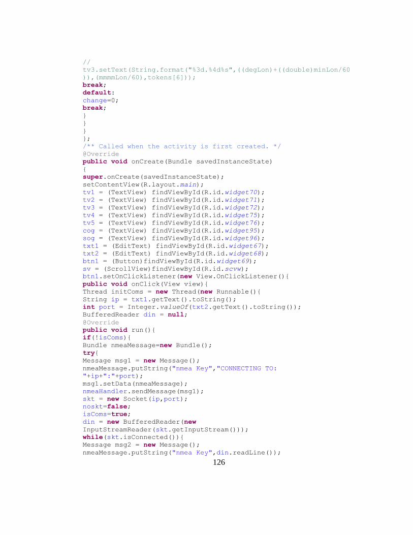
126
//
tv3.setText(String.format("%3d.%4d%s",((degLon)+((double)minLon/60
)),(mmmmLon/60),tokens[6]));
break;
default:
change=0;
break;
}
}
}
};
/** Called when the activity is first created. */
@Override
public void onCreate(Bundle savedInstanceState)
{
super.onCreate(savedInstanceState);
setContentView(R.layout.main);
tv1 = (TextView) findViewById(R.id.widget70);
tv2 = (TextView) findViewById(R.id.widget71);
tv3 = (TextView) findViewById(R.id.widget72);
tv4 = (TextView) findViewById(R.id.widget75);
tv5 = (TextView) findViewById(R.id.widget76);
cog = (TextView) findViewById(R.id.widget95);
sog = (TextView) findViewById(R.id.widget96);
txt1 = (EditText) findViewById(R.id.widget67);
txt2 = (EditText) findViewById(R.id.widget68);
btn1 = (Button)findViewById(R.id.widget69);
sv = (ScrollView)findViewById(R.id.scvw);
btn1.setOnClickListener(new View.OnClickListener(){
public void onClick(View view){
Thread initComs = new Thread(new Runnable(){
String ip = txt1.getText().toString();
int port = Integer.valueOf(txt2.getText().toString());
BufferedReader din = null;
@Override
public void run(){
if(!isComs){
Bundle nmeaMessage=new Bundle();
try{
Message msg1 = new Message();
nmeaMessage.putString("nmea Key","CONNECTING TO:
"+ip+":"+port);
msg1.setData(nmeaMessage);
nmeaHandler.sendMessage(msg1);
skt = new Socket(ip,port);
noskt=false;
isComs=true;
din = new BufferedReader(new
InputStreamReader(skt.getInputStream()));
while(skt.isConnected()){
Message msg2 = new Message();
nmeaMessage.putString("nmea Key",din.readLine());
127
msg2.setData(nmeaMessage);
nmeaHandler.sendMessage(msg2);
}
}
catch(Exception e){
Message msg2 = new Message();
nmeaMessage.putString("nmea Key","A network error has
occured:\n"+e.toString()+
"\nPlease ensure the IP address and port
are correct and try again\n");
msg2.setData(nmeaMessage);
nmeaHandler.sendMessage(msg2);
isComs=false;
}
}else if(skt.isConnected()){
Message msg = new Message();
Bundle nmeaMessage=new Bundle();
nmeaMessage.putString("nmea Key","\n!!!ALREADY CONNECTED!!!\n"+
"PRESS+HOLD Connect button to DISCONNECT.\n");
msg.setData(nmeaMessage);
nmeaHandler.sendMessage(msg);
}
}
});
initComs.start();
}
});
btn1.setOnLongClickListener(new View.OnLongClickListener(){
public boolean onLongClick(View view){
if(!isComs){
tv1.append("\nNOT CONNECTED\n");
return true;
}else{
try{
skt.close();
tv1.append("\nDISCONNECTED\n");
isComs=false;
}
catch(Exception e){
tv1.append("\nOn skt.close():\n"+e.toString());
}
return true;
}
}
});
btn2 = (Button)findViewById(R.id.widget73);
btn2.setOnClickListener(new View.OnClickListener(){
public void onClick(View view){
change++;
}
});
class Steering {private boolean MARK, PORT, STBD;}
128
final Steering steeringMode = new Steering();
final ToggleButton togglebutton[] ={
(ToggleButton) findViewById(R.id.widget77),
(ToggleButton) findViewById(R.id.widget78),
(ToggleButton) findViewById(R.id.widget79),
(ToggleButton) findViewById(R.id.widget80)};
togglebutton[0].setOnClickListener(new OnClickListener(){
@Override
public void onClick(View v){
if (((ToggleButton) v).isChecked()){
try{PrintWriter dout = new PrintWriter(new BufferedWriter
(new OutputStreamWriter(skt.getOutputStream())),true);
dout.println("$$$");
dout.println("set sys output 0\r");
dout.println("exit\r");
steeringMode.MARK = true;
// if(togglebutton[1].isChecked()){Togglebutton[2].setChecked();}
Toast.makeText(getApplicationContext(),"IN
AUTO",Toast.LENGTH_SHORT).show();
tv4.setText(""+latMk);
tv5.setText(""+lonMk);
}
catch(Exception e){
Toast.makeText(getBaseContext(),
e.getMessage(),Toast.LENGTH_SHORT).show();
}
}else{
try{PrintWriter dout = new PrintWriter(new BufferedWriter
(new OutputStreamWriter(skt.getOutputStream())),true);
dout.println("$$$");
dout.println("set sys output 0x100\r");
dout.println("exit\r");
steeringMode.MARK = false;
Toast.makeText(getApplicationContext(),"IN
MANUAL",Toast.LENGTH_SHORT).show();
}
catch(Exception e){
Toast.makeText(getBaseContext(),
e.getMessage(),Toast.LENGTH_SHORT).show();
}
}
}
});
togglebutton[1].setOnClickListener(new OnClickListener(){
@Override
public void onClick(View v){
if (((ToggleButton) v).isChecked()){
isLogging = true;
File dpblogDirectory = new
File(Environment.getExternalStorageDirectory().getPath()+"/dpblog/"
);
dpblogDirectory.mkdirs();
129
Calendar calLog = Calendar.getInstance();
String logSeq =
""+(1+calLog.get(Calendar.MONTH))+calLog.get(Calendar.DAY_OF_MONTH)
+calLog.get(Calendar.H
OUR_OF_DAY)
+calLog.get(Calendar.MINUTE)+calLog.get(Calendar.SECOND);
dpblog =
Environment.getExternalStorageDirectory().getPath()+"/dpblog/"+logS
eq+".txt";
Toast.makeText(getApplicationContext(),"logging to file
"+dpblog,Toast.LENGTH_LONG).show();
}else{
isLogging = false;
}
}
});
togglebutton[2].setOnClickListener(new OnClickListener(){
@Override
public void onClick(View v){
if (((ToggleButton) v).isChecked()){
steeringMode.PORT = true;
if(!steeringMode.MARK){
if(steeringMode.PORT && steeringMode.STBD){
try{PrintWriter dout = new PrintWriter(new BufferedWriter
(new OutputStreamWriter(skt.getOutputStream())),true);
dout.println("$$$");
dout.println("set sys output 0x182\r");
dout.println("exit\r");
//tv1.append(steeringMode.PORT+"set sys output
0x182"+steeringMode.STBD);
Toast.makeText(getApplicationContext(),"ALL
AHEAD!",Toast.LENGTH_SHORT).show();
}
catch(Exception e){
Toast.makeText(getBaseContext(), "Not
connected"+e.getMessage(),Toast.LENGTH_SHORT).show();
}
}else if(steeringMode.PORT && !steeringMode.STBD){
try{PrintWriter dout = new PrintWriter(new BufferedWriter
(new OutputStreamWriter(skt.getOutputStream())),true);
dout.println("$$$");
dout.println("set sys output 0x180\r");
dout.println("exit\r");
//tv1.append(steeringMode.PORT+" set sys output
0x180"+steeringMode.STBD);
Toast.makeText(getApplicationContext(),"TURNING
RIGHT!",Toast.LENGTH_SHORT).show();
}
catch(Exception e){
Toast.makeText(getBaseContext(), "Not connected"+
e.getMessage(),Toast.LENGTH_SHORT).show();
}
130
}
}else{
Toast.makeText(getApplicationContext(),"Can't! DPB IS IN
AUTO",Toast.LENGTH_SHORT).show();
}
}
else if(steeringMode.MARK){
Toast.makeText(getApplicationContext(),"Can't! DPB IS IN
AUTO",Toast.LENGTH_SHORT).show();
}else{
steeringMode.PORT=false;
try{PrintWriter dout = new PrintWriter(new BufferedWriter
(new OutputStreamWriter(skt.getOutputStream())),true);
dout.println("$$$");
dout.println("set sys output 0x100\r");
dout.println("exit\r");
// tv1.append(steeringMode.PORT+"set sys output
0x100"+steeringMode.STBD);
Toast.makeText(getApplicationContext(),"ALL
STOP!",Toast.LENGTH_SHORT).show();
}
catch(Exception e){
Toast.makeText(getBaseContext(),"Not connected"+
e.getMessage(),Toast.LENGTH_SHORT).show();
}
}
}
});
togglebutton[3].setOnClickListener(new OnClickListener(){
@Override
public void onClick(View v){
if (((ToggleButton) v).isChecked()){
steeringMode.STBD = true;
if(!steeringMode.MARK){
if(steeringMode.STBD && steeringMode.PORT){
try{PrintWriter dout = new PrintWriter(new BufferedWriter
(new OutputStreamWriter(skt.getOutputStream())),true);
dout.println("$$$");
dout.println("set sys output 0x182\r");
dout.println("exit\r");
// tv1.append(steeringMode.PORT+"set sys output
0x182"+steeringMode.STBD);
Toast.makeText(getApplicationContext(),"ALL
AHEAD!",Toast.LENGTH_SHORT).show();
}
catch(Exception e){
Toast.makeText(getBaseContext(), "Not
connected"+e.getMessage(),Toast.LENGTH_SHORT).show();
}
}else if(steeringMode.STBD && !steeringMode.PORT){
try{PrintWriter dout = new PrintWriter(new BufferedWriter
(new OutputStreamWriter(skt.getOutputStream())),true);
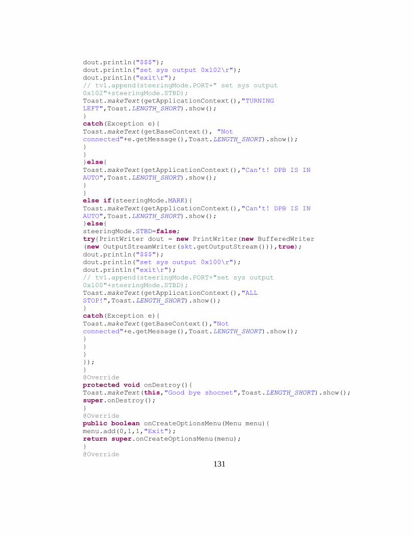
131
dout.println("$$$");
dout.println("set sys output 0x102\r");
dout.println("exit\r");
// tv1.append(steeringMode.PORT+" set sys output
0x102"+steeringMode.STBD);
Toast.makeText(getApplicationContext(),"TURNING
LEFT",Toast.LENGTH_SHORT).show();
}
catch(Exception e){
Toast.makeText(getBaseContext(), "Not
connected"+e.getMessage(),Toast.LENGTH_SHORT).show();
}
}
}else{
Toast.makeText(getApplicationContext(),"Can't! DPB IS IN
AUTO",Toast.LENGTH_SHORT).show();
}
}
else if(steeringMode.MARK){
Toast.makeText(getApplicationContext(),"Can't! DPB IS IN
AUTO",Toast.LENGTH_SHORT).show();
}else{
steeringMode.STBD=false;
try{PrintWriter dout = new PrintWriter(new BufferedWriter
(new OutputStreamWriter(skt.getOutputStream())),true);
dout.println("$$$");
dout.println("set sys output 0x100\r");
dout.println("exit\r");
// tv1.append(steeringMode.PORT+"set sys output
0x100"+steeringMode.STBD);
Toast.makeText(getApplicationContext(),"ALL
STOP!",Toast.LENGTH_SHORT).show();
}
catch(Exception e){
Toast.makeText(getBaseContext(),"Not
connected"+e.getMessage(),Toast.LENGTH_SHORT).show();
}
}
}
});
}
@Override
protected void onDestroy(){
Toast.makeText(this,"Good bye shocnet",Toast.LENGTH_SHORT).show();
super.onDestroy();
}
@Override
public boolean onCreateOptionsMenu(Menu menu){
menu.add(0,1,1,"Exit");
return super.onCreateOptionsMenu(menu);
}
@Override

132
public boolean onOptionsItemSelected(MenuItem item){
if(item.getItemId()==1){
if(noskt){finish();}
else{
try{
skt.close();
}
catch(Exception e){
Toast.makeText(getBaseContext(),"Error closing
socket:"+e.getMessage(),Toast.LENGTH_SHORT).show();
}
finish();
}
}
return super.onOptionsItemSelected(item);
}
}
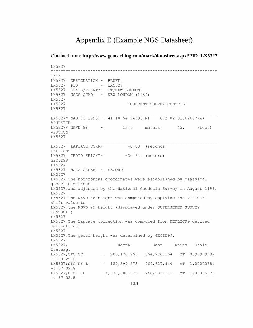
133
Appendix E (Example NGS Datasheet)
Obtained from: http://www.geocaching.com/mark/datasheet.aspx?PID=LX5327
LX5327
*******************************************************************
****
LX5327 DESIGNATION - BLUFF
LX5327 PID - LX5327
LX5327 STATE/COUNTY- CT/NEW LONDON
LX5327 USGS QUAD - NEW LONDON (1984)
LX5327
LX5327 *CURRENT SURVEY CONTROL
LX5327
___________________________________________________________________
LX5327* NAD 83(1996)- 41 18 54.94996(N) 072 02 01.62697(W)
ADJUSTED
LX5327* NAVD 88 - 13.6 (meters) 45. (feet)
VERTCON
LX5327
___________________________________________________________________
LX5327 LAPLACE CORR- -0.83 (seconds)
DEFLEC99
LX5327 GEOID HEIGHT- -30.64 (meters)
GEOID99
LX5327
LX5327 HORZ ORDER - SECOND
LX5327
LX5327.The horizontal coordinates were established by classical
geodetic methods
LX5327.and adjusted by the National Geodetic Survey in August 1998.
LX5327
LX5327.The NAVD 88 height was computed by applying the VERTCON
shift value to
LX5327.the NGVD 29 height (displayed under SUPERSEDED SURVEY
CONTROL.)
LX5327
LX5327.The Laplace correction was computed from DEFLEC99 derived
deflections.
LX5327
LX5327.The geoid height was determined by GEOID99.
LX5327
LX5327; North East Units Scale
Converg.
LX5327;SPC CT - 206,170.759 364,770.164 MT 0.99999037
+0 28 29.6
LX5327;SPC NY L - 129,399.875 464,627.840 MT 1.00002781
+1 17 09.8
LX5327;UTM 18 - 4,578,000.379 748,285.176 MT 1.00035873
+1 57 33.5

134
LX5327;UTM 19 - 4,578,196.098 246,058.196 MT 1.00039370
-2 00 14.3
LX5327
LX5327: Primary Azimuth Mark
Grid Az
LX5327:SPC CT - NEW LONDON LEDGE LIGHTHOUSE 253
36 58.8
LX5327:SPC NY L - NEW LONDON LEDGE LIGHTHOUSE 252
48 18.6
LX5327:UTM 18 - NEW LONDON LEDGE LIGHTHOUSE 252
07 54.9
LX5327:UTM 19 - NEW LONDON LEDGE LIGHTHOUSE 256
05 42.7
LX5327
LX5327|------------------------------------------------------------
---------|
LX5327| PID Reference Object Distance
Geod. Az |
LX5327|
dddmmss.s |
LX5327| LX5256 PRENTIS WHITE CHIMNEY APPROX. 0.8 KM
0144647.9 |
LX5327| LW3386 MYSTIC ELEV TANK APPROX. 6.7 KM
0441734.9 |
LX5327| LW3390 NOANK SPIRE APPROX. 4.1 KM
0731322.7 |
LX5327| LX5289 LONG POINT TANK APPROX. 2.1 KM
0852736.5 |
LX5327| LW3410 SIMMONS CHIMNEY APPROX. 9.6 KM
1053958.8 |
LX5327| LX5281 MANDALAY FLAGPOLE APPROX. 2.0 KM
1080849.8 |
LX5327| LW3413 COAST GUARD CUPOLA APPROX. 8.3 KM
1152640.8 |
LX5327| LX5282 WESTERNS FLAGPOLE APPROX. 2.1 KM
1155932.6 |
LX5327| LX5280 WESTERNS CHIMNEY APPROX. 2.1 KM
1161938.6 |
LX5327| LW3423 CLUBHOUSE CHIMNEY APPROX. 8.2 KM
1181451.6 |
LX5327| LX5253 MUMFORD POINT 448.987 METERS
1375411.3 |
LX5327| LX5320 CAMP TABOR BARN CUPOLA APPROX. 6.8 KM
1553018.3 |
LX5327| LX5255 FORT WRIGHT SILVER TANK APPROX. 6.4 KM
1783118.2 |
LX5327| LX5193 SEAFLOWER REEF LIGHT APPROX. 2.1 KM
1784849.9 |
LX5327| LX5367 3501 A PT 225.630 METERS
25253 |
LX5327| LX5215 NEW LONDON LEDGE LIGHTHOUSE APPROX. 3.8 KM
2540528.4 |
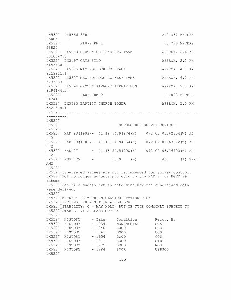
135
LX5327| LX5366 3501 219.387 METERS
25405 |
LX5327| BLUFF RM 1 13.736 METERS
25829 |
LX5327| LX5209 GROTON CG TRNG STA TANK APPROX. 2.6 KM
2810047.3 |
LX5327| LX5197 GAYS SILO APPROX. 2.2 KM
3153638.2 |
LX5327| LX5205 MAX POLLOCK CO STACK APPROX. 4.1 KM
3213821.6 |
LX5327| LX5207 MAX POLLOCK CO ELEV TANK APPROX. 4.0 KM
3233033.8 |
LX5327| LX5194 GROTON AIRPORT AIRWAY BCN APPROX. 2.0 KM
3294144.2 |
LX5327| BLUFF RM 2 16.063 METERS
34741 |
LX5327| LX5325 BAPTIST CHURCH TOWER APPROX. 3.5 KM
3521815.1 |
LX5327|------------------------------------------------------------
---------|
LX5327
LX5327 SUPERSEDED SURVEY CONTROL
LX5327
LX5327 NAD 83(1992)- 41 18 54.94874(N) 072 02 01.62604(W) AD(
) 2
LX5327 NAD 83(1986)- 41 18 54.94954(N) 072 02 01.63122(W) AD(
) 2
LX5327 NAD 27 - 41 18 54.59900(N) 072 02 03.36400(W) AD(
) 2
LX5327 NGVD 29 - 13.9 (m) 46. (f) VERT
ANG
LX5327
LX5327.Superseded values are not recommended for survey control.
LX5327.NGS no longer adjusts projects to the NAD 27 or NGVD 29
datums.
LX5327.See file dsdata.txt to determine how the superseded data
were derived.
LX5327
LX5327_MARKER: DS = TRIANGULATION STATION DISK
LX5327_SETTING: 80 = SET IN A BOULDER
LX5327_STABILITY: C = MAY HOLD, BUT OF TYPE COMMONLY SUBJECT TO
LX5327+STABILITY: SURFACE MOTION
LX5327
LX5327 HISTORY - Date Condition Recov. By
LX5327 HISTORY - 1934 MONUMENTED CGS
LX5327 HISTORY - 1940 GOOD CGS
LX5327 HISTORY - 1943 GOOD CGS
LX5327 HISTORY - 1954 GOOD CGS
LX5327 HISTORY - 1971 GOOD CTDT
LX5327 HISTORY - 1975 GOOD NGS
LX5327 HISTORY - 1984 POOR USPSQD
LX5327
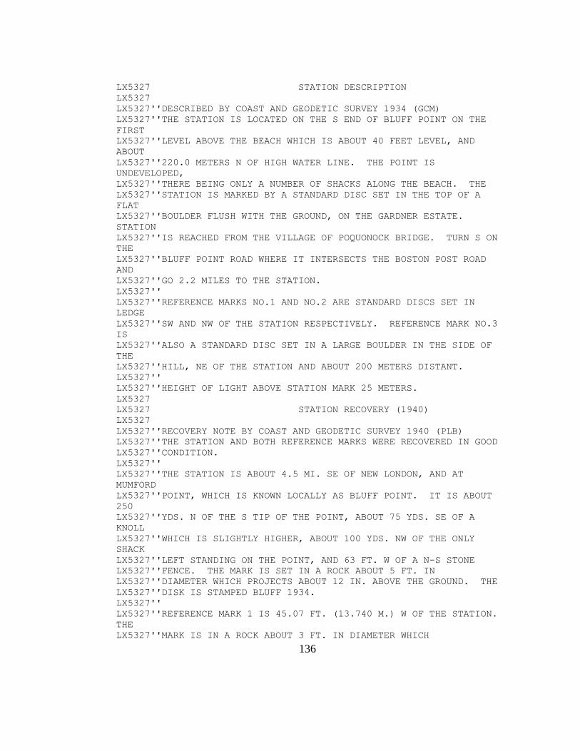
136
LX5327 STATION DESCRIPTION
LX5327
LX5327''DESCRIBED BY COAST AND GEODETIC SURVEY 1934 (GCM)
LX5327''THE STATION IS LOCATED ON THE S END OF BLUFF POINT ON THE
FIRST
LX5327''LEVEL ABOVE THE BEACH WHICH IS ABOUT 40 FEET LEVEL, AND
ABOUT
LX5327''220.0 METERS N OF HIGH WATER LINE. THE POINT IS
UNDEVELOPED,
LX5327''THERE BEING ONLY A NUMBER OF SHACKS ALONG THE BEACH. THE
LX5327''STATION IS MARKED BY A STANDARD DISC SET IN THE TOP OF A
FLAT
LX5327''BOULDER FLUSH WITH THE GROUND, ON THE GARDNER ESTATE.
STATION
LX5327''IS REACHED FROM THE VILLAGE OF POQUONOCK BRIDGE. TURN S ON
THE
LX5327''BLUFF POINT ROAD WHERE IT INTERSECTS THE BOSTON POST ROAD
AND
LX5327''GO 2.2 MILES TO THE STATION.
LX5327''
LX5327''REFERENCE MARKS NO.1 AND NO.2 ARE STANDARD DISCS SET IN
LEDGE
LX5327''SW AND NW OF THE STATION RESPECTIVELY. REFERENCE MARK NO.3
IS
LX5327''ALSO A STANDARD DISC SET IN A LARGE BOULDER IN THE SIDE OF
THE
LX5327''HILL, NE OF THE STATION AND ABOUT 200 METERS DISTANT.
LX5327''
LX5327''HEIGHT OF LIGHT ABOVE STATION MARK 25 METERS.
LX5327
LX5327 STATION RECOVERY (1940)
LX5327
LX5327''RECOVERY NOTE BY COAST AND GEODETIC SURVEY 1940 (PLB)
LX5327''THE STATION AND BOTH REFERENCE MARKS WERE RECOVERED IN GOOD
LX5327''CONDITION.
LX5327''
LX5327''THE STATION IS ABOUT 4.5 MI. SE OF NEW LONDON, AND AT
MUMFORD
LX5327''POINT, WHICH IS KNOWN LOCALLY AS BLUFF POINT. IT IS ABOUT
250
LX5327''YDS. N OF THE S TIP OF THE POINT, ABOUT 75 YDS. SE OF A
KNOLL
LX5327''WHICH IS SLIGHTLY HIGHER, ABOUT 100 YDS. NW OF THE ONLY
SHACK
LX5327''LEFT STANDING ON THE POINT, AND 63 FT. W OF A N-S STONE
LX5327''FENCE. THE MARK IS SET IN A ROCK ABOUT 5 FT. IN
LX5327''DIAMETER WHICH PROJECTS ABOUT 12 IN. ABOVE THE GROUND. THE
LX5327''DISK IS STAMPED BLUFF 1934.
LX5327''
LX5327''REFERENCE MARK 1 IS 45.07 FT. (13.740 M.) W OF THE STATION.
THE
LX5327''MARK IS IN A ROCK ABOUT 3 FT. IN DIAMETER WHICH
137
LX5327''PROJECTS ABOUT 6 IN. ABOVE THE GROUND. THE DISK IS STAMPED
LX5327''BLUFF NO 1 1934.
LX5327''
LX5327''REFERENCE MARK 2 IS 52.72 FT. (16.069 M.) N OF THE STATION.
THE
LX5327''MARK IS IN A ROCK ABOUT 5 FT. IN DIAMETER WHICH
LX5327''PROJECTS ABOUT 12 IN. ABOVE THE GROUND. THE DISK IS
STAMPED
LX5327''BLUFF NO 2 1934.
LX5327''
LX5327''NEW LONDON LEDGE LIGHTHOUSE IS A GOOD AZIMUTH MARK. IT IS
LX5327''ABOUT 2-1/2 MI. W OF THE STATION, ON THE W SIDE OF
SOUTHWEST
LX5327''LEDGE, AT THE E SIDE OF THE ENTRANCE TO NEW LONDON HARBOR.
THE
LX5327''FINIAL OVER THE LIGHT WAS OBSERVED UPON.
LX5327''
LX5327''A 4-FT. STAND AT THIS STATION WILL SEE 4-FT. STANDS AT
STATIONS
LX5327''MYSTIC AND NORTH HILL.
LX5327
LX5327 STATION RECOVERY (1943)
LX5327
LX5327''RECOVERY NOTE BY COAST AND GEODETIC SURVEY 1943 (FN)
LX5327''STATION WAS RECOVERED AS DESCRIBED, AND THE MARKS WERE
FOUND IN
LX5327''GOOD CONDITION. THE SHACK MENTIONED IN THE 1940
DESCRIPTION NO
LX5327''LONGER STANDS. A NEW DESCRIPTION FOLLOWS--
LX5327''
LX5327''STATION IS LOCATED ABOUT 4.5 MI. SE OF NEW LONDON, ON
MUMFORD
LX5327''POINT, WHICH IS KNOWN LOCALLY AS BLUFF POINT. IT IS ABOUT
250
LX5327''YDS. N OF THE S TIP OF THE POINT, ABOUT 75 YDS. SE OF A
KNOLL WHICH
LX5327''IS SLIGHTLY HIGHER, AND ABOUT 63 FT. W OF A N-S STONE
LX5327''FENCE. THE STATION MARK IS STAMPED BLUFF 1934 AND
LX5327''PROJECTS ABOUT 12 IN.
LX5327''
LX5327''REFERENCE MARK 1 IS W OF THE STATION. IT IS STAMPED
LX5327''BLUFF NO 1 1934 AND PROJECTS ABOUT 6 IN.
LX5327''
LX5327''REFERENCE MARK 2 IS N OF THE STATION. IT IS STAMPED
LX5327''BLUFF 2 1934 AND PROJECTS ABOUT 12 IN.
LX5327''
LX5327''TO REACH THE STATION FROM THE TOLL GATE OF THE NEW BRIDGE
LX5327''ACROSS THE THAMES RIVER AT NEW LONDON, GO E ON U.S. HIGHWAY
1 FOR
LX5327''3.15 MI. TO THE INTERSECTION WITH DEPOT ROAD IN THE VILLAGE
OF
138
LX5327''POQUONOCK BRIDGE. TURN RIGHT ON DEPOT ROAD, AND GO 0.3 MI.
TO
LX5327''THE END OF THE PAVED STREET AND A FORK. TAKE THE RIGHT
FORK
LX5327''(GRAVEL ROAD), PASS UNDER A BRIDGE AND GO 0.45 MI. TO A
GATE
LX5327''WHICH IS JUST PAST A SINGLE RAILROAD TRACK. GO THROUGH THE
LX5327''GATE AND FOLLOW A WOODS ROAD FOR 0.5 MI. TO A FORK. TAKE
THE
LX5327''RIGHT FORK AND GO 0.45 MI. TO A REVERSE Y. CONTINUE FOR
0.55
LX5327''MI. TO THE TOP OF A KNOLL AND THE STATION.
LX5327''
LX5327''NOTE--THE R.M. 1 DISTANCE FOR 1943 WAS CAREFULLY CHECKED
AND
LX5327''THE 1940 DISTANCE WAS FOUND TO BE IN ERROR AS SHOWN.
LX5327
LX5327 STATION RECOVERY (1954)
LX5327
LX5327''RECOVERY NOTE BY COAST AND GEODETIC SURVEY 1954 (LFW)
LX5327''STATION AND REFERENCE MARKS 1 AND 2 WERE RECOVERED IN GOOD
LX5327''CONDITION. REFERENCE MARK 3 WAS NOT RECOVERED. THE 1940
LX5327''RECOVERY NOTE BY P.L.B. IS ADEQUATE AND COMPLETE, EXCEPT
THAT
LX5327''THERE ARE NO SHACKS NOW STANDING IN THE VICINITY OF THE
LX5327''STATION. THE 1954 DISTANCE FOR REFERENCE MARK 1 WAS
CAREFULLY
LX5327''CHECKED, AND THE 1943 DISTANCE WAS FOUND TO BE IN ERROR AS
LX5327''SHOWN.
LX5327
LX5327 STATION RECOVERY (1971)
LX5327
LX5327''RECOVERY NOTE BY CT DEPT OF TRANSP 1971
LX5327''THE STATION AND REFERENCE MARKS WERE FOUND IN GOOD
CONDITION. TO
LX5327''REACH FROM GROTON AT THE NORTH ROAD EXIT ON ROUTE 95, GO
SOUTH
LX5327''FOR 0.65 MILE ON NORTH ROAD TO A FORK, BEAR RIGHT, GO 0.55
MILE
LX5327''TO THE INTERSECTION OF FORT HILL ROAD, CONTINUE STRAIGHT ON
LX5327''DEPOT ROAD, FOR 0.35 MILE TO RAILROAD TRACKS, GO STRAIGHT
UNDER
LX5327''THE RAILROAD BRIDGE FOR 0.9 MILE ON GRAVEL ROAD PAST GROTON
LX5327''TOWN BEACH TO A GATE, CONTINUE STRAIGHT IN BLUFF POINT
STATE
LX5327''PARK FOR 1.15 MILES TO A FOOT PATH. THE STATION IS 200
FEET
LX5327''NORTH OF THE DIRT ROAD AND 80 FEET EAST OF THE FOOT PATH.
A
LX5327''WITNESS POST IS IN THE AREA.
LX5327
LX5327 STATION RECOVERY (1975)
139
LX5327
LX5327''RECOVERY NOTE BY NATIONAL GEODETIC SURVEY 1975 (HRR)
LX5327''THE STATION, REFERENCE MARKS 1 AND 2 WERE RECOVERED IN GOOD
LX5327''CONDITION. THE DISTANCE TO REFERENCE MARK 1 CHECKED THE
1940
LX5327''MEASUREMENT AND THE DISTANCE TO REFERENCE MARK 2 CHECKED
THE
LX5327''1943 MEASUREMENT. THE DIRECTION TO BOTH REFERENCE MARKS
LX5327''CHECKED. CONNECTICUT GEODETIC SURVEY MARK 3501 WAS USED AS
AN
LX5327''AZIMUTH MARK AT THIS TIME. A COMPLETE NEW DESCRIPTION
FOLLOWS.
LX5327''
LX5327''STATION IS ABOUT 4-1/2 MILES SOUTHEAST OF NEW LONDON, 3
MILES
LX5327''EAST OF OCEAN BEACH, 1/4 MILE WEST OF THE WATERS EDGE ON
BLUFF
LX5327''POINT AND ON PROPERTY OWNED BY THE STATE FOREST AND PARK
SERVICE.
LX5327''
LX5327''TO REACH THE STATION FROM THE JUNCTION OF U.S. HIGHWAY 1
AND
LX5327''DEPOT ROAD AT THE TOWN OFFICES IN GROTON, GO SOUTH ON DEPOT
LX5327''ROAD FOR 0.25 MILE TO THE JUNCTION OF INDUSTRIAL ROAD ON
THE
LX5327''LEFT AND GROTON TOWN BEACH ROAD STRAIGHT AHEAD. CONTINUE
LX5327''SOUTHERLY ON GROTON TOWN BEACH ROAD FOR 0.8 MILE TO THE
GROTON
LX5327''TOWN BEACH. CONTINUE ACROSS THE BEACH AND GO SOUTHERLY ON
A
LX5327''WOODS ROAD FOR 0.9 MILE TO A FORK. (TO REACH 3501 (CGS)
FROM
LX5327''HERE, TAKE RIGHT FORK AND GO WESTERLY ON MAIN TRAVELED ROAD
LX5327''FOR 0.2 MILE TO A HIGH KNOLL AT THE WATERS EDGE AND THE
MARK
LX5327''ON THE KNOLL AS DESCRIBED). TAKE LEFT FORK AND GO
SOUTHWEST
LX5327''ON A DIM TRACK ROAD FOR 0.15 MILE TO A SMALL OPEN AREA AND
LX5327''THE STATION ON THE LEFT AS DESCRIBED.
LX5327''
LX5327''STATION MARK, STAMPED BLUFF 1934, IS A STANDARD DISK
CEMENTED
LX5327''IN A DRILL HOLE IN OUTCROPPING BEDROCK WHICH PROJECTS ABOUT
6
LX5327''INCHES ABOVE THE GROUND SURFACE AND IS ABOUT 3 BY 4 FEET IN
LX5327''SIZE. IT IS 83 FEET EAST OF CENTER OF THE TRACK ROAD, 12
FEET
LX5327''NORTH OF AN 8-INCH APPLE TREE AND 4.5 FEET NORTHEAST OF A
LX5327''METAL WITNESS POST.
LX5327''
LX5327''REFERENCE MARK 1, STAMPED BLUFF NO 1 1934, IS A STANDARD
DISK
140
LX5327''CEMENTED IN A DRILL HOLE IN OUTCROPPING BEDROCK WHICH
PROJECTS
LX5327''ABOUT 4 INCHES ABOVE THE GROUND SURFACE AND IS ABOUT 2 BY 3
LX5327''FEET IN SIZE. IT IS 42 FEET WEST OF THE METAL WITNESS POST
LX5327''AT THE STATION MARK AND 38 FEET EAST OF CENTER OF THE TRACK
ROAD.
LX5327''
LX5327''REFERENCE MARK 2, STAMPED BLUFF NO 2 1934, IS A STANDARD
LX5327''DISK CEMENTED IN A DRILL HOLE IN OUTCROPPING BEDROCK WHICH
LX5327''PROJECTS ABOUT 10 INCHES ABOVE THE GROUND SURFACE AND IS
LX5327''ABOUT 2 BY 3 FEET IN SIZE. IT IS 55.5 FEET NORTH OF THE
LX5327''METAL WITNESS POST AT THE STATION MARK AND 7.5 FEET NORTH
OF A
LX5327''TWIN TRUNKED APPLE TREE.
LX5327''
LX5327''AZIMUTH MARK, STAMPED 3501, IS A U.S. COAST AND GEODETIC
LX5327''SURVEY AND STATE SURVEY DISK SET IN A 6 BY 6 INCH CONCRETE
LX5327''POST WHICH PROJECTS ABOUT 6 INCHES ABOVE THE GROUND
LX5327''SURFACE. IT IS 30 FEET EAST OF THE WEST EDGE OF A BLUFF
LX5327''AT THE WATERS EDGE, 27 FEET NORTH OF CENTER OF A BOULDER
LX5327''WHICH IS ABOUT 5 BY 7 FEET IN SIZE AND 26 FEET WEST OF
CENTER
LX5327''OF A TRACK ROAD.
LX5327''
LX5327''HEIGHT OF LIGHT ABOVE STATION MARK 4 FEET.
LX5327''
LX5327''AIRLINE DISTANCE AND DIRECTION FROM NEAREST TOWN
LX5327''3 MILES EAST OF OCEAN BEACH.
LX5327
LX5327 STATION RECOVERY (1984)
LX5327
LX5327''RECOVERY NOTE BY US POWER SQUADRON 1984 (BWR)
LX5327''BLUFF 1934 DAMAGED.
LX5327''
LX5327''RECOVERED AS DESCRIBED - EXCEPT THE 1943 REFERENCE GROTON
COAST
LX5327''GUARD TRAINING STATION, WATER TANK. TANK WAS DEMOLISHED IN
AUGUST
LX5327''1983 WITNESS POST IN AREA OK. R. M. NO. 1 AND R. M. NO. 2
FOUND
LX5327''IN GOOD COND.
LX5327''
LX5327''NOTE--R. M. NO. 3 FOUND IN GOOD CONDITION IN AN AREA GROWN
OVER
LX5327''HEAVY IN BRUSH AND WEEDS. A SEARCH OF OVER TWO HOURS
RECOVERED
LX5327''IT. IT IS THE MOST PROMINENT BOULDER IN THE AREA.