Hybrid optimization model for conjunctive use of surface

Article

Hybrid optimization model for conjunctive use of surface and

groundwater resources in water deficit irrigation system

Karthikeyan MoothampalayamSampathkumar1,*, Saravanan Ramasamy1, Balamurugan Ramasubbu1, Hamid Reza

Pourghasemi2, Saravanan Karuppanan1 and Balaji Lakshminarayanan1

1 Centre for Water Resources, Anna University, Chennai, India

[email protected] (S.R.); [email protected] (B.R.); [email protected] (S.K);

[email protected] (B.L.); 2 Department of Natural Resources and Environmental Engineering, College of Agriculture, Shiraz University,

Shiraz 71441-65186, Iran; [email protected] (H.R.P.)

* Correspondence: [email protected](K.M.);

Abstract: Increasing demand for food production with limited available water resources pose the

threat to agricultural activities. The conjunctive allocation of water resources maximizes the net ben-

efit of farmers efficiently. In this study, a novel hybrid optimization model was developed based on

a genetic algorithm (GA), bacterial foraging optimization (BFO) and ant colony optimization (ACO)

to maximize the net benefit of water deficit Sathanur reservoir command. The GA-based optimiza-

tion model considered crop-related physical and economical parameters to derive optimal cropping

patterns for three different conjunctive use policies and further allocation of surface and groundwa-

ter for different crops are enhanced with the BFO. The allocation of surface and groundwater for the

head, middle and tail reach obtained from BFO is considered as input to ACO as a guiding mecha-

nism to attain an optimal cropping pattern. Comparing the average productivity values Policy 3

(3.665 Rs/m3) has better values relating to Policy 1 (3.662 Rs/m3) and Policy 2 (3.440 Rs/m3). Thus,

the developed novel hybrid optimization model (GA-BFO-ACO) is very promising to enhance the

farmer's net income as well as for the command area water conservation and can be replicated in

other irrigated regions of the globe to overcome chronic land and water problems.

Keywords: conjunctive use; cropping pattern; genetic algorithm; bacterial foraging optimization;

ant colony optimization; hybrid optimization; productivity

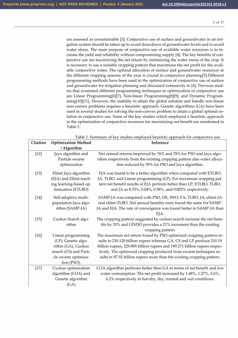
1. Introduction

Population increment and demand for food resources impose a serious threat to wa-

ter resources, as a 60% increase in food requirement is expected in the year 2050[1]. Cli-

mate change increased the rainfall intensity and reduced the number of rainy days in an

occurring year which leads to flood and drought without proper management of available

rainfall which pose risk to human lives[2]. In many developing nations 90% of water with-

drawn for irrigation purposes and extraction of groundwater about 15- 35% for irrigation

Preprints (www.preprints.org) | NOT PEER-REVIEWED | Posted: 4 January 2021 doi:10.20944/preprints202101.0018.v1

© 2021 by the author(s). Distributed under a Creative Commons CC BY license.

mailto:[email protected]






https://doi.org/10.20944/preprints202101.0018.v1

http://creativecommons.org/licenses/by/4.0/

2 of 17

are assessed as unsustainable [3]. Conjunctive use of surface and groundwater in an irri-

gation system should be taken up to avoid drawdown of groundwater levels and to avoid

water stress. The main purpose of conjunctive use of available water resources is to in-

crease the yield and reliability without compromising supply [4]. The key benefits of con-

junctive use are maximizing the net return by minimizing the water stress of the crop. It

is necessary to use a suitable cropping pattern that maximizes the net profit for the avail-

able conjunctive water. The optimal allocation of surface and groundwater resources at

the different cropping seasons of the year is crucial in conjunctive planning[5].Different

programming methods have been used in the optimization of conjunctive use of surface

and groundwater for irrigation planning and discussed extensively in [4]. Previous stud-

ies that examined different programming techniques in optimization of conjunctive use

are Linear Programming[6][7], Non-linear Programming[8][9], and Dynamic Program-

ming[10][11]. However, the inability to attain the global solution and handle non-linear

non-convex problems requires a heuristic approach. Genetic algorithms (GA) have been

used in several studies for solving the non-convex problem to attain a global optimal so-

lution in conjunctive use. Some of the key studies which employed a heuristic approach

in the optimization of conjunctive resources for maximizing net benefit are mentioned in

Table 1.

Table 1. Summary of key studies employed heuristic approach for conjunctive use

Citation Optimization Method

/ Algorithm

Inference

[12] Jaya algorithm and

Particle swarm

optimization

Net annual returns improved by 76% and 78% for PSO and Jaya algo-

rithm respectively from the existing cropping pattern also water alloca-

tion reduced by 39% for PSO and Jaya algorithm.

[13] Elitist Jaya algorithm

(EJA) and Elitist teach-

ing learning-based op-

timization (ETLBO)

EJA was found to be a better algorithm when compared with ETLBO,

JA, TLBO, and Linear programming (LP). For maximum cropping pat-

tern net benefit results of EJA perform better than LP, ETLBO, TLBO,

and JA as 8.33%, 0.04%, 0.58%, and 0.002% respectively.

[14] Self-adaptive multi-

population Jaya algo-

rithm (SAMP-JA)

SAMP-JA was compared with PSO, DE, IWO, FA, TLBO, JA, elitist-JA

and elitist-TLBO. Net annual benefits were found the same for SAMP-

JA and EJA. The rate of convergence was found better in SAMP-JA than

EJA.

[15] Cuckoo Search algo-

rithm

The cropping pattern suggested by cuckoo search increase the net bene-

fits by 33% and LINDO provides a 21% increment than the existing

cropping pattern.

[16] Linear programming

(LP), Genetic algo-

rithm (GA), Cuckoo

search (CS) and Parti-

cle swarm optimiza-

tion (PSO).

The maximum net return found by PSO optimized cropping pattern re-

sults in 230.120 billion rupees whereas GA, CS and LP produce 210.19

billion rupees, 229.895 billion rupees and 199.271 billion rupees respec-

tively. The optimized cropping produced from swarm techniques re-

sults in 97.92 billion rupees more than the existing cropping pattern.

[17] Cuckoo optimization

algorithm (COA) and

Genetic algorithm

(GA)

COA algorithm performs better than GA in terms of net benefit and low

water consumption. The net profit increased by 1.48%, 1.27%, 2.6%,

6.2% respectively in hot-dry, dry, normal and wet conditions.



3 of 17

[18] Genetic algorithm

(GA)

Conjunctive use of surface and groundwater resources is optimized us-

ing a genetic algorithm (GA) for two scenarios. For scenario – I, 24

MCM of water was saved with a reduction in net financial return by

22%. For scenario- II, the net revenue increased in dry years when com-

pared with normal and wet years.

However, as discussed in the literature much of the early work centers around the

comparison of meta-heuristic algorithm performance in the optimization of cropping pat-

terns which maximize the net benefits of farmers. In this study, a novel hybrid optimiza-

tion approach is employed for the conjunctive use of surface and groundwater to maxim-

ize the economic benefit by optimizing cropping patterns. Considering the effectiveness

of meta-heuristic algorithms, a hybrid optimization model which comprises of Genetic

Algorithm (GA), Bacterial Foraging Optimization (BFO) and Ant Colony Optimization

(ACO) was developed. The developed model would maximize the farmers' net benefit by

conjunctively using the surface water from reservoir release and groundwater resources

at the head, middle and tail reach of the Sathanur reservoir command for three different

cropping seasons. The developed model comprises of three stages i) Cropping area opti-

mization based on genetic algorithm ii) Optimization of surface and groundwater alloca-

tion conjunctively using BFO iii) Maximizing the net benefit of farmers using ACO.

2. Materials and Methods

2.1. Study Area

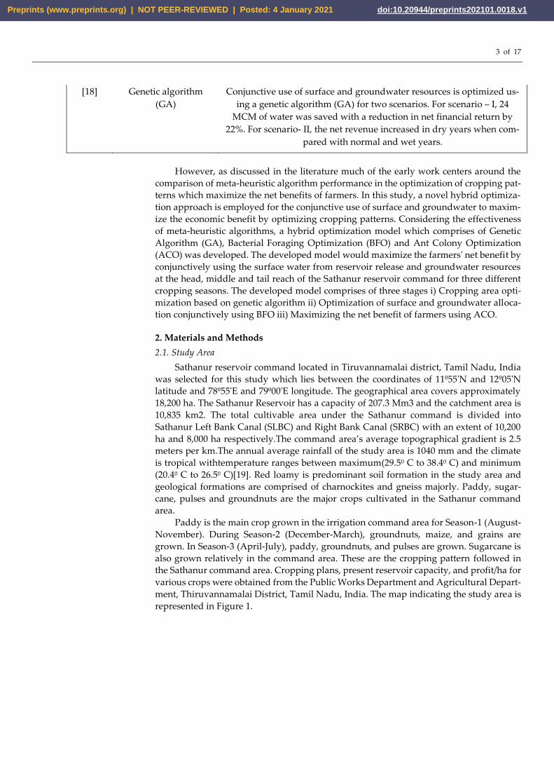
Sathanur reservoir command located in Tiruvannamalai district, Tamil Nadu, India

was selected for this study which lies between the coordinates of 11º55'N and 12º05'N

latitude and 78º55'E and 79º00'E longitude. The geographical area covers approximately

18,200 ha. The Sathanur Reservoir has a capacity of 207.3 Mm3 and the catchment area is

10,835 km2. The total cultivable area under the Sathanur command is divided into

Sathanur Left Bank Canal (SLBC) and Right Bank Canal (SRBC) with an extent of 10,200

ha and 8,000 ha respectively.The command area’s average topographical gradient is 2.5

meters per km.The annual average rainfall of the study area is 1040 mm and the climate

is tropical withtemperature ranges between maximum(29.50 C to 38.40 C) and minimum

(20.40 C to 26.50 C)[19]. Red loamy is predominant soil formation in the study area and

geological formations are comprised of charnockites and gneiss majorly. Paddy, sugar-

cane, pulses and groundnuts are the major crops cultivated in the Sathanur command

area.

Paddy is the main crop grown in the irrigation command area for Season-1 (August-

November). During Season-2 (December-March), groundnuts, maize, and grains are

grown. In Season-3 (April-July), paddy, groundnuts, and pulses are grown. Sugarcane is

also grown relatively in the command area. These are the cropping pattern followed in

the Sathanur command area. Cropping plans, present reservoir capacity, and profit/ha for

various crops were obtained from the Public Works Department and Agricultural Depart-

ment, Thiruvannamalai District, Tamil Nadu, India. The map indicating the study area is

represented in Figure 1.



4 of 17

Figure 1. Sathanur Command Area Map

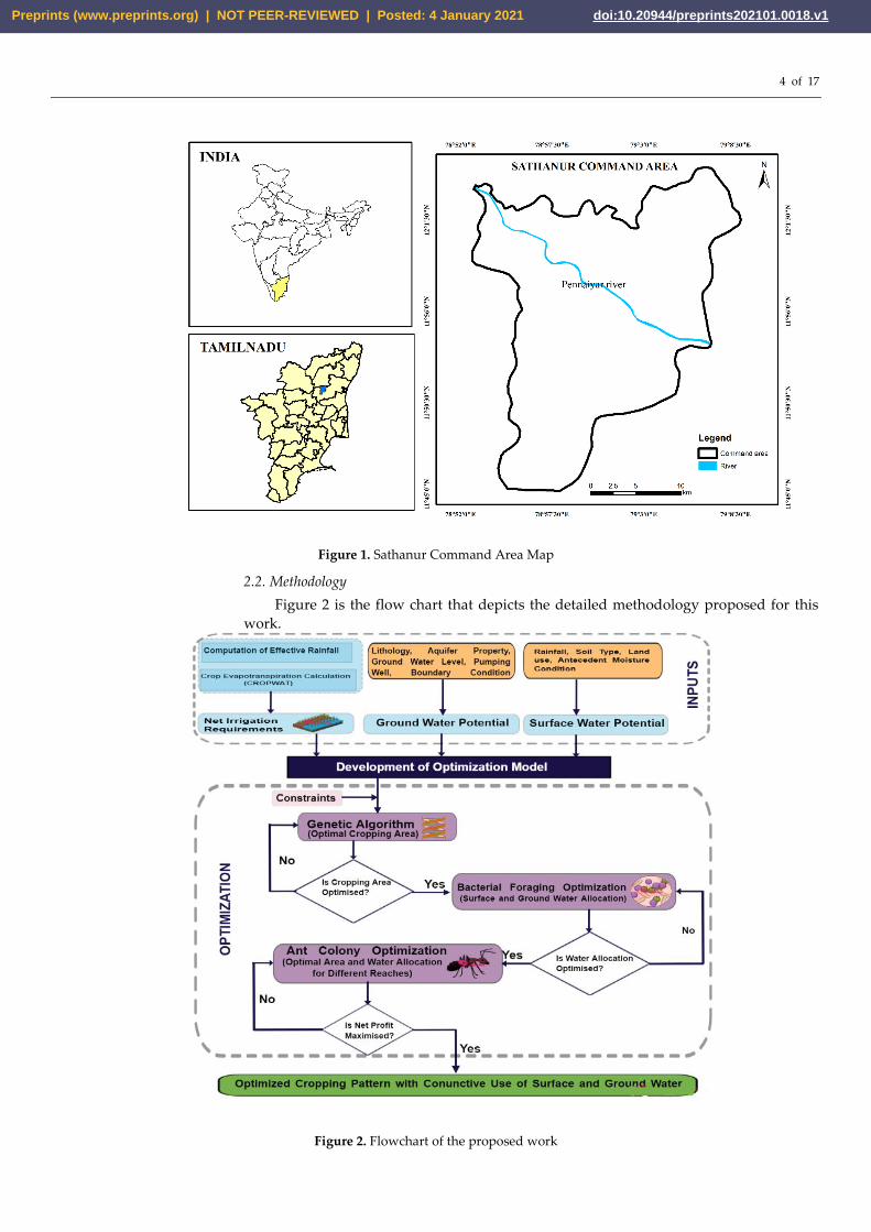
2.2. Methodology

Figure 2 is the flow chart that depicts the detailed methodology proposed for this

work.

Figure 2. Flowchart of the proposed work



5 of 17

2.3. Irrigation Water Requirements

The net irrigation requirement (NIR) is referred as the amount of water required by

a crop for augmenting the rainfall to meet the crop's evapotranspiration (𝑬𝑻𝒄) without

compromising the yield of the crop. There are several techniques are available to compute

the reference crop evapotranspiration (𝑬𝑻𝟎) and crop evapotranspiration (𝑬𝑻𝒄) of the

crop. [20][21]:

𝐸𝑇𝑐 = 𝐾𝑐 × 𝐸𝑇0 (1)

where 𝐸𝑇𝑐 represents the crop evapotranspiration in mm/day; 𝐾𝑐 and 𝐸𝑇0 repre-

sent the crop coefficient and reference evapotranspiration in mm/day respectively. The

following equation given by [22] is used to calculate the NIR of a crop:

𝑁𝐼𝑅 = 𝐸𝑇𝑐 – 𝐸𝑅 (2)

where 𝑁𝐼𝑅 is measured in mm/month and 𝐸𝑅 is the measurement of effective rain-

fall in mm/month.

CROPWAT is an effective decision tool proposed by FAO [23] for irrigation planning

and management based on a daily water balance. It is used to compute ET0 and data re-

quired are duration of various crop growth stages, crop coefficients, date of sowing/plant-

ing, initial and final root depths, and crop yield response factors. In the case of paddy, the

depth of water required for land preparation and puddling need to be specified [24]. Cli-

matic data (monthly average) crop and soil data were used to estimate the ETc values

and the NIR of crops in the command area.

2.4. Estimation of Surface and Ground Water Potential

The prediction of surface water volume for the rainfall depth from any catchment is

possible with a well-established method called Soil Conservation Service Curve Number

(SCS-CN). SCS-CN technique was proposed in the year 1964 by the USDA who deter-

mined that a single CN accounts for numerous factors that affect the runoff [25]. [26] sug-

gests that the SCS-CN technique was a very useful method to estimate precipitation excess

(runoff), by considering cumulative precipitation, antecedent soil moisture condition,

land use, and land cover. The groundwater level fluctuation method recommended by the

groundwater estimation committee [27] is widely used in the Indian context to calculate

the net groundwater recharge for the command area during the monsoon season. Source

[28] suggested that the groundwater level fluctuation method is useful in estimating the

net groundwater recharge using the observed fluctuations in the groundwater level from

14 wells for a period of 15 years (2004-2018).

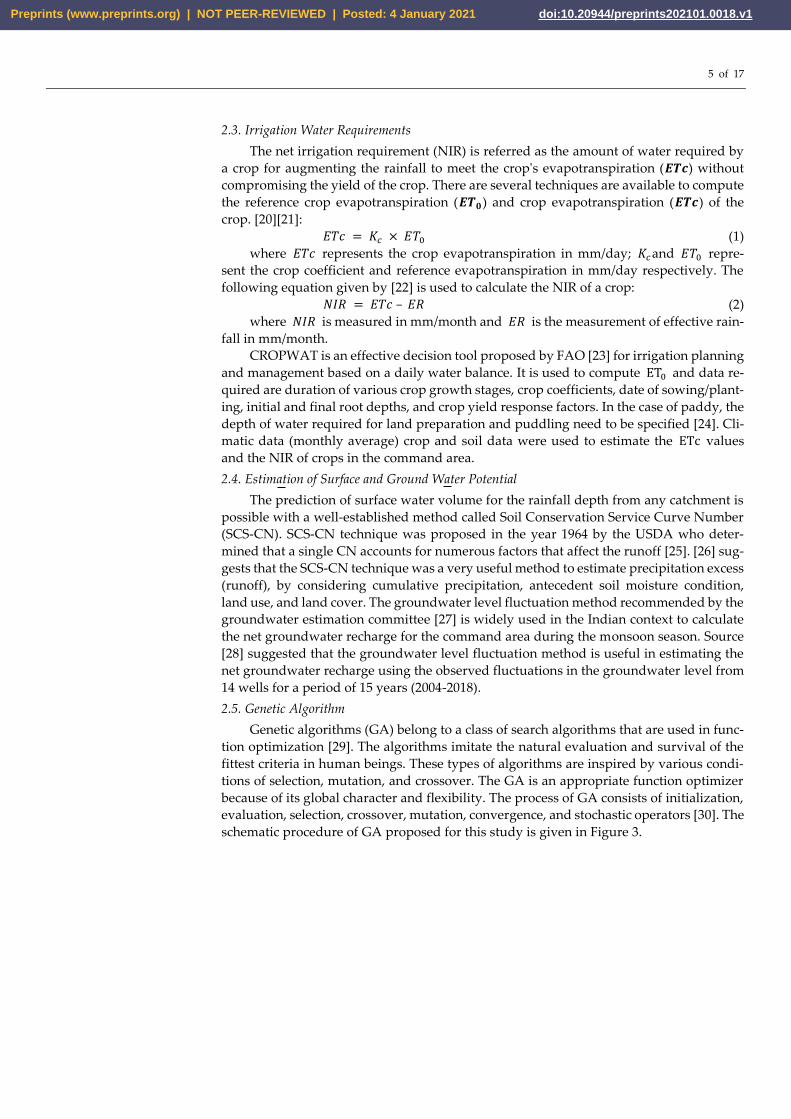
2.5. Genetic Algorithm

Genetic algorithms (GA) belong to a class of search algorithms that are used in func-

tion optimization [29]. The algorithms imitate the natural evaluation and survival of the

fittest criteria in human beings. These types of algorithms are inspired by various condi-

tions of selection, mutation, and crossover. The GA is an appropriate function optimizer

because of its global character and flexibility. The process of GA consists of initialization,

evaluation, selection, crossover, mutation, convergence, and stochastic operators [30]. The

schematic procedure of GA proposed for this study is given in Figure 3.



6 of 17

Figure 3. Schematic procedure of GA proposed for this study.

There are several parameters required to run a genetic algorithm. The GA algorithm

uses the iterative technique to create an optimal solution to the given problem by appro-

priately adjusting the ideal parameter [31]. The optimization process using a genetic algo-

rithm was carried out using a soft computing technique [32]. Source [33] has used an elitist

strategy for obtaining the optimal solution using GA. The parameters used in the GA are

population size, crossover, and mutation rates of 500, 0.9, and 0.01 respectively to obtain

the optimal solution. The elitist selection procedure with a generation gap of 0.98 is

adopted.

2.6. Optimization Model

The main objective is to formulate an optimization model for maximum net returns

by optimally utilizing the surface and groundwater resources (total water) for the crops

that are grown (Farmer Preference Constraints) in the command area. The most important

part of the optimization model is to assign the non-negative constraints to achieve the

global optimum for the objective function. The non-negative constraints are incorporated

because decision variables should not produce a negative value and the smallest value

could be zero.

Maximize Z = ∑ 𝐴𝑗𝑛𝑗=1 × 𝑃 (3)

Subject to

∑ 𝐴𝑗𝑊𝑗 ≤ 𝑇𝑊𝑅

𝑛

𝑗=1

(4)

∑ 𝐴𝑗

𝑛

𝑗=1

≤ 𝑇𝐶𝐴 (5)

∑ 𝑇𝐶𝐴, 𝑇𝑊𝑅, Aj ≥ 0 (6)

where 𝐴𝑗and 𝑃 is the area under irrigation and net return for jth crop respectively.

𝑊𝑗 is the water requirement for jth crop, 𝑇𝑊𝑅 is the total water (surface and groundwa-

ter) resources available and 𝑇𝐶𝐴 is the total cultivable area under irrigation.

The main function of GA is to arrive an optimal cropping area of the Sathanur com-

mand with constraints such as type of crop, crop water requirement, available surface and

groundwater resources. The output of GA is used as input to Bacterial Foraging Optimi-

zation (BFO) for optimizing the source (Surface and Groundwater) allocation for the con-

junctive use of water.

2.7. Bacterial Foraging Optimization (BFO) Algorithm

In Bacterial foraging optimization technique presented by [34], a set of bacteria at-

tempts to accomplish optimum threshold value by involving stages chemotaxis, swarm-

Decision Variable

(Command area, Crop,

Reservoir capacity,

Groundwater, Profit/ha)

Crossover and

mutation

Offspring

Generation of various

alternative cropping plans

Fitness Function

Select the best fit decision for

maximizing the net benefit

Evolution of

Offspring



7 of 17

ing, reproduction, elimination and dispersal. The main idea of BFO is imitating the chem-

otactic movement of virtual bacteria in the search domain. Each bacterium generates set

of best possible values of parameters iteratively. Progressively, all the bacteria congregate

to the global optimum threshold value. The bacteria have a choice either to tumble by a

tumble or a tumble followed by a run/swim in the chemotaxis stage. In the process of

swarming, each bacterium signals other bacterium to swarm together via attractants. To

keep the swarm size constant, the least healthy bacteria die and the healthier bacteria is

asexually split into two bacteria, which are then placed in the same location in the repro-

duction stage. Whereas in the final stage, any bacterium is either eliminated or dispersed

from the set to a random space in the process of optimization. This stage mainly helps the

bacteria to attaining the global optimum solution. If i represents the bacterium position

and J(i) is the objective function, then J(i) < 0; nutrient rich , J(i) = 0; neutral, and J(i) > 0;

toxic. Bacteria tries to mount up the concentration of nutrient to find the minor values of

J(i). And also, they try to find way out of neutral media and to avoid toxic substances. The

BFO algorithm is modified to find the optimal allocation of surface and groundwater re-

sources.

2.7.1.Bacterial Foraging Optimization Algorithm for the Proposed Study

The control parameters proposed of the Bacterial Foraging Optimization Algorithm

for this study are (i) Number of bacterium (S) = 50, (ii) Maximum number of steps (Ns) =

4, (iii) Number of chemotactic steps (Nc) = 100, (iv) Number of reproduction steps (Nre) =

4, (v) Number of elimination-dispersal steps (Ned) = 2, (vi) Probability (Ped) = 0.25 and (vii)

Step size C(i) = 0.1

Step - 1: S, Nc, Ns, Nre, Ned, Ped (Intializing the Parameters) and the C(i), (i =1, 2…, S).

Choose the initial value for control variable (θi )cropping area. The control variables

(θi) are randomly distributed across the search space. Once the θi is computed, the P value

is updated automatically and reaches the termination when it reaches the maximum spec-

ified iterations.

Step - 2: l= l+1 (Elimination-Dispersal loop)

Step - 3: k= k+1 (Reproduction loop)

Step - 4: j= j+1 (Chemo taxis loop)

(a) Chemo tactic step for bacterium ‘i= 1,2,…S’ as follows:

(b) Let J(i,j,k,l) = Compute water allocation

(c) J(i,j,k,l)=J(i,j,k,l)+Jcc(θi (j,k,l),P(j,k,l))

(d) To find better surface and groundwater allocation Jlast = J (i,j,k,l)

(e) Tumble: Δ(i) ϵ Rp with each element generate a random vector, R is a real num-

ber. Generate a random number on [0,1]for the steps Δm(i), m= 1, 2,….,p.

(f) Modify the water source allocation

𝛳𝑖(𝑗 + 1, 𝑘, 𝑙) = 𝛳𝑖(𝑗, 𝑘, 𝑙) + 𝐶(𝑖)∆(𝑖)

√∆𝑇(𝑖)∆(𝑖) (7)

This depicts step size C(i) for bacterium I in the direction of the tumble

(vii) Compute the updated water allocation J(i,j+1,k,l)

(viii) Swim.

Swim function is to allocate the positive increment of cropping area until satisfying

the surface and groundwater availability

(ix) Take next bacterium (i+1) if i ≠ S (i.e., possibility of increment in area allocation

for surface water and groundwater simultaneously)

Step - 5: If j<Nc, repeat from step 3. Continue chemotaxis process, till all the surface

and groundwater sources are allocated for each crop.

Step - 6:

(a) Jhealth (i) be the total allocation of water resources. Compute for the given k and l,

and for each i=1, 2…., S,



8 of 17

𝐽ℎ𝑒𝑎𝑙𝑡ℎ𝑖 = ∑ 𝐽(𝑖, 𝑗, 𝑘, 𝑙)

𝑁𝑐+1

𝑗=1

(8)

(b) The Sr bacterium (allocated surface and groundwater) with the least productivity

Jhealth values die and the healthy (Sr ) bacteria with the best values split.

Step - 7: If k<Nre, go to step 2. Once specified reproduction steps not reached.

Step - 8: Elimination-Dispersal

For i=1, 2..., S with probability Ped, to eliminate and disperse each bacterium in the

random space on the optimization domain. If l <Ned, then go to step 1, else end.

The BFO algorithm results in an optimal allocation of surface and groundwater re-

sources considering the input from Genetic algorithm as optimum cropping pattern and

the result of BFO is the input for Ant Colony Optimization (ACO) guided search algorithm

to distribute resources to head, middle and tail command area to obtain the maximum net

profit.

2.8. Ant Colony Optimization (ACO) For Optimal Conjunctive Use of Surface and Groundwater

The Ant Colony Optimization system[35] was first developed by the behaviour of

ants to find the shortest route between food and nest. ACO is a branch of swarm intelli-

gence and group of ants with its social behaviour used to solve optimization problems.

While travelling ants deposit pheromones and the other ants follow in their trial. Each

trial of an ant is strongly followed by pheromone deposit along possible path. The phero-

mone density during each trial is an indirect communication and reinforcement learning.

In this study, an ACO algorithm is developed to maximize the net profit from the

distribution of surface and groundwater to the head, middle and tail reach of the com-

mand area for different crop seasons. The developed method is a mathematical optimiza-

tion approach that uses a guided search technique. The search domain is flexible between

the possible available surface and groundwater. The. The cropping area is discretized and

assigned as ants for the search domain. The ants are allowed to move in the reaches of the

head, middle and tail. The different sources of water (surface water and groundwater) are

obtained from the BFO and are used for maximizing the net profit for the entire cropping

season. Each ant will explore the possibility of maximizing the net profit through the area

allocated in the head, middle and tail reach with the available surface water and ground-

water.

The objective function of ACO for the net profit maximization and is given:

𝑀𝐴𝑋𝐼𝑀𝐼𝑍𝐸 𝑍 = ∑ ∑ ∑ 𝐶𝐴

𝑠𝑜𝑢𝑟𝑐𝑒𝑠

𝑘=1

𝑟𝑒𝑎𝑐ℎ𝑒𝑠

𝑗=1

𝑠𝑒𝑎𝑠𝑜𝑛𝑠

𝑖=1

(𝑖, 𝑗, 𝑘, 𝑐𝑝)

∗ 𝑁𝑃(𝑐𝑝, 𝑘)

(9)

where, Z is the net profit function; CA is the area of the crop; NP is the net profit; i is

the season varies from 1 to 3; j is the reaches (head, middle and tail); k is the source of

water supply (surface water and groundwater) and cp is the cropping pattern area

(Paddy, sugarcane, groundnut, maize, grains and pulses)

The crop area is divided into a segment of varieties such as Paddy, sugarcane,

groundnut, maize, grains and pulses. These crop areas are commanded in the reaches of

the head, middle and tail in the form of discretized quantity. To facilitate the search by

each ant, the surface and groundwater distribution for the different season is proportion-

ally made for head, middle and tail reaches for the different crops. Three different policies

are considered for the distribution of surface and groundwater and the details are given

in Table 2.



9 of 17

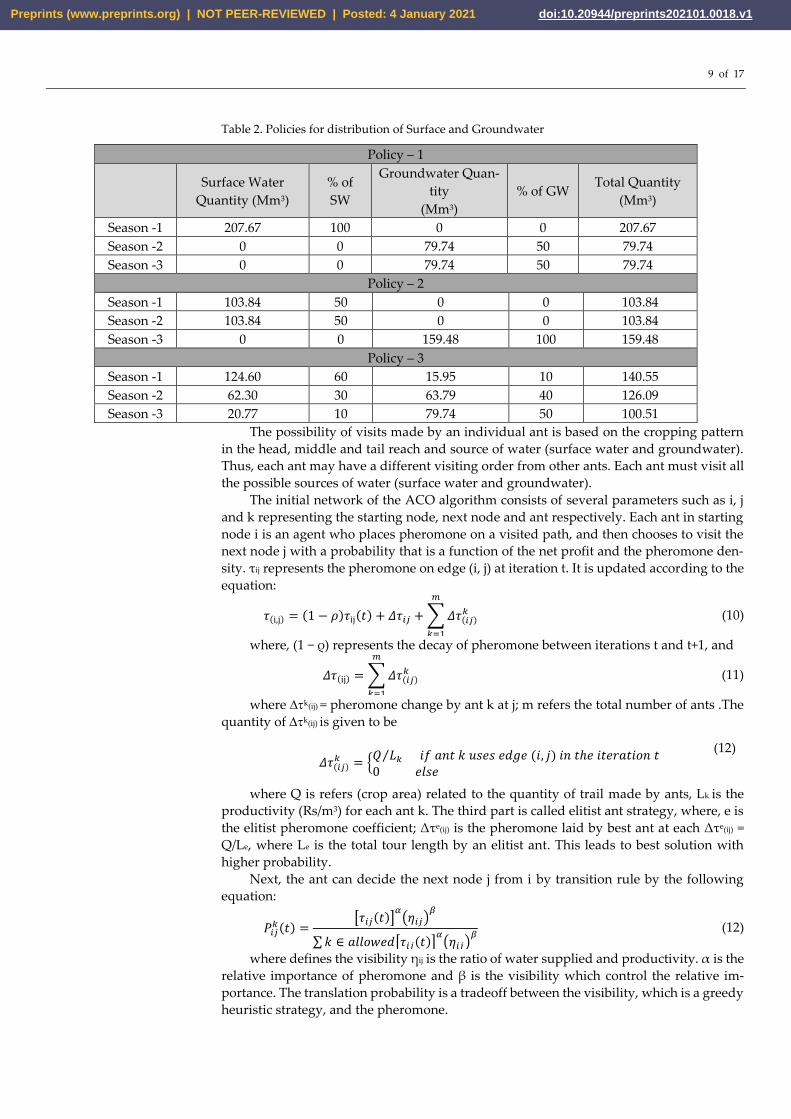
Table 2. Policies for distribution of Surface and Groundwater

Policy – 1

Surface Water

Quantity (Mm3)

% of

SW

Groundwater Quan-

tity

(Mm3)

% of GW Total Quantity

(Mm3)

Season -1 207.67 100 0 0 207.67

Season -2 0 0 79.74 50 79.74

Season -3 0 0 79.74 50 79.74

Policy – 2

Season -1 103.84 50 0 0 103.84

Season -2 103.84 50 0 0 103.84

Season -3 0 0 159.48 100 159.48

Policy – 3

Season -1 124.60 60 15.95 10 140.55

Season -2 62.30 30 63.79 40 126.09

Season -3 20.77 10 79.74 50 100.51

The possibility of visits made by an individual ant is based on the cropping pattern

in the head, middle and tail reach and source of water (surface water and groundwater).

Thus, each ant may have a different visiting order from other ants. Each ant must visit all

the possible sources of water (surface water and groundwater).

The initial network of the ACO algorithm consists of several parameters such as i, j

and k representing the starting node, next node and ant respectively. Each ant in starting

node i is an agent who places pheromone on a visited path, and then chooses to visit the

next node j with a probability that is a function of the net profit and the pheromone den-

sity. τij represents the pheromone on edge (i, j) at iteration t. It is updated according to the

equation:

𝜏(i,j) = (1 − 𝜌)𝜏ij(𝑡) + 𝛥𝜏𝑖𝑗 + ∑ 𝛥𝜏(𝑖𝑗)𝑘

𝑚

𝑘=1

(10)

where, (1 − ρ) represents the decay of pheromone between iterations t and t+1, and

𝛥𝜏(ij) = ∑ 𝛥𝜏(𝑖𝑗)𝑘

𝑚

𝑘=1

(11)

where k(ij) = pheromone change by ant k at j; m refers the total number of ants .The

quantity of k(ij) is given to be

where Q is refers (crop area) related to the quantity of trail made by ants, Lk is the

productivity (Rs/m3) for each ant k. The third part is called elitist ant strategy, where, e is

the elitist pheromone coefficient; Δτe(ij) is the pheromone laid by best ant at each Δτe(ij) =

Q/Le, where Le is the total tour length by an elitist ant. This leads to best solution with

higher probability.

Next, the ant can decide the next node j from i by transition rule by the following

equation:

𝑃𝑖𝑗𝑘 (𝑡) =

[𝜏𝑖𝑗(𝑡)]𝛼

(𝜂𝑖𝑗)𝛽

∑ 𝑘 ∈ 𝑎𝑙𝑙𝑜𝑤𝑒𝑑[𝜏𝑖𝑗(𝑡)]𝛼

(𝜂𝑖𝑗)𝛽

(12)

where defines the visibility ηij is the ratio of water supplied and productivity. α is the

relative importance of pheromone and β is the visibility which control the relative im-

portance. The translation probability is a tradeoff between the visibility, which is a greedy

heuristic strategy, and the pheromone.

𝛥𝜏(𝑖𝑗)𝑘 = {

𝑄 𝐿𝑘⁄ 𝑖𝑓 𝑎𝑛𝑡 𝑘 𝑢𝑠𝑒𝑠 𝑒𝑑𝑔𝑒 (𝑖, 𝑗) 𝑖𝑛 𝑡ℎ𝑒 𝑖𝑡𝑒𝑟𝑎𝑡𝑖𝑜𝑛 𝑡0 𝑒𝑙𝑠𝑒

(12)



10 of 17

The above steps are repeated for each set of cropping seasons to achieve the maxi-

mum net profit with conjunctive use of surface and groundwater. All mentioned compu-

tational experiments were coded in C++ using Microsoft Visual Studio 2015 platform.

3. Results

This section summarises and discusses the main findings of the work. To optimize

the net profit of the Sathanur command area, a Hybrid optimization model was devel-

oped. The net return of each crop, Total water availability and the Net Irrigation Require-

ment were calculated and given as input parameters.

3.1. Net Return of Crops

The net profit of crops per hectare was estimated by including the market price of

crops , crop yield and cost of production. The major crop expenses such as seed cost, land

preparation cost and labour cost have been obtained from the Tamil Nadu Agriculture

University and Agricultural Marketing Information Center (directorate of marketing and

inspection), Thiruvannamalai District, Tamil Nadu, India. Profit per hectare for Paddy,

Sugarcane, Groundnut, Maize, Pulses and Grains are 22156, 38000, 19136, 14000, 8000,

10000 rupees respectively.

3.2. Total Water Availability

The SCS runoff equation was developed to estimate the total storm runoff. Weighted

CN-II was estimated as 86 by taking into the consideration of hydrological soil group - B

(moderately low runoff potential) and cultivated land area. The daily rainfall for 15 years

was used to compute the daily runoff.

The total surface water is 282.22 Mm3, which includes the reservoir capacity (207.67

Mm3) and the surface runoff of the command area. The quantity of surface water consid-

ered for the optimization model is 207.67 Mm3 (reservoir capacity) and the groundwater

quantity as 159.49 Mm3 (obtained via the water table fluctuation method); thus, the total

water available is 367.16 Mm3 which is considered for the hybrid optimization model.

3.3. Crop Water Requirement

To estimate the crop water requirement (CWR) for each crop (paddy, sugarcane,

groundnut, maize, grains, and pulses) CROPWAT was used and the values were 1.2 m, 2

m, 0.42 m, 0.3 m, 0.2 m, and 0.187 m respectively. Paddy and sugarcane have the highest

CWR compared to other crops.

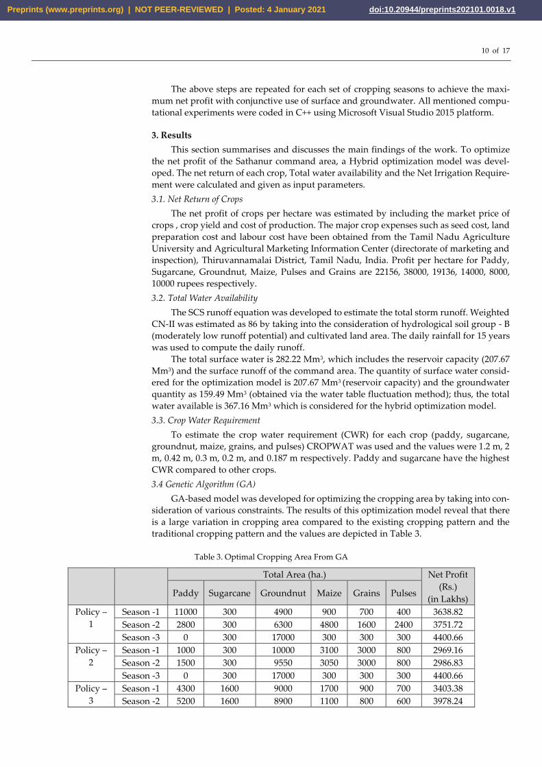
3.4 Genetic Algorithm (GA)

GA-based model was developed for optimizing the cropping area by taking into con-

sideration of various constraints. The results of this optimization model reveal that there

is a large variation in cropping area compared to the existing cropping pattern and the

traditional cropping pattern and the values are depicted in Table 3.

Table 3. Optimal Cropping Area From GA

Total Area (ha.) Net Profit

(Rs.)

(in Lakhs) Paddy Sugarcane Groundnut Maize Grains Pulses

Policy –

1

Season -1 11000 300 4900 900 700 400 3638.82

Season -2 2800 300 6300 4800 1600 2400 3751.72

Season -3 0 300 17000 300 300 300 4400.66

Policy –

2

Season -1 1000 300 10000 3100 3000 800 2969.16

Season -2 1500 300 9550 3050 3000 800 2986.83

Season -3 0 300 17000 300 300 300 4400.66

Policy –

3

Season -1 4300 1600 9000 1700 900 700 3403.38

Season -2 5200 1600 8900 1100 800 600 3978.24



11 of 17

Season -3 0 1600 14400 1000 600 600 4017.31

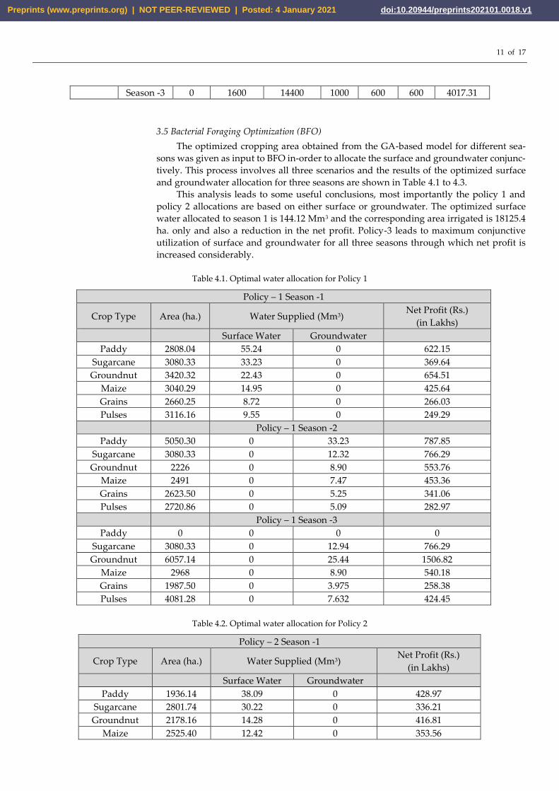
3.5 Bacterial Foraging Optimization (BFO)

The optimized cropping area obtained from the GA-based model for different sea-

sons was given as input to BFO in-order to allocate the surface and groundwater conjunc-

tively. This process involves all three scenarios and the results of the optimized surface

and groundwater allocation for three seasons are shown in Table 4.1 to 4.3.

This analysis leads to some useful conclusions, most importantly the policy 1 and

policy 2 allocations are based on either surface or groundwater. The optimized surface

water allocated to season 1 is 144.12 Mm3 and the corresponding area irrigated is 18125.4

ha. only and also a reduction in the net profit. Policy-3 leads to maximum conjunctive

utilization of surface and groundwater for all three seasons through which net profit is

increased considerably.

Table 4.1. Optimal water allocation for Policy 1

Policy – 1 Season -1

Crop Type Area (ha.) Water Supplied (Mm3) Net Profit (Rs.)

(in Lakhs)

Surface Water Groundwater

Paddy 2808.04 55.24 0 622.15

Sugarcane 3080.33 33.23 0 369.64

Groundnut 3420.32 22.43 0 654.51

Maize 3040.29 14.95 0 425.64

Grains 2660.25 8.72 0 266.03

Pulses 3116.16 9.55 0 249.29


Paddy 5050.30 0 33.23 787.85

Sugarcane 3080.33 0 12.32 766.29

Groundnut 2226 0 8.90 553.76

Maize 2491 0 7.47 453.36

Grains 2623.50 0 5.25 341.06

Pulses 2720.86 0 5.09 282.97


Paddy 0 0 0 0

Sugarcane 3080.33 0 12.94 766.29

Groundnut 6057.14 0 25.44 1506.82

Maize 2968 0 8.90 540.18

Grains 1987.50 0 3.975 258.38

Pulses 4081.28 0 7.632 424.45



Crop Type Area (ha.) Water Supplied (Mm3) Net Profit (Rs.)

(in Lakhs)


Paddy 1936.14 38.09 0 428.97

Sugarcane 2801.74 30.22 0 336.21

Groundnut 2178.16 14.28 0 416.81

Maize 2525.40 12.42 0 353.56



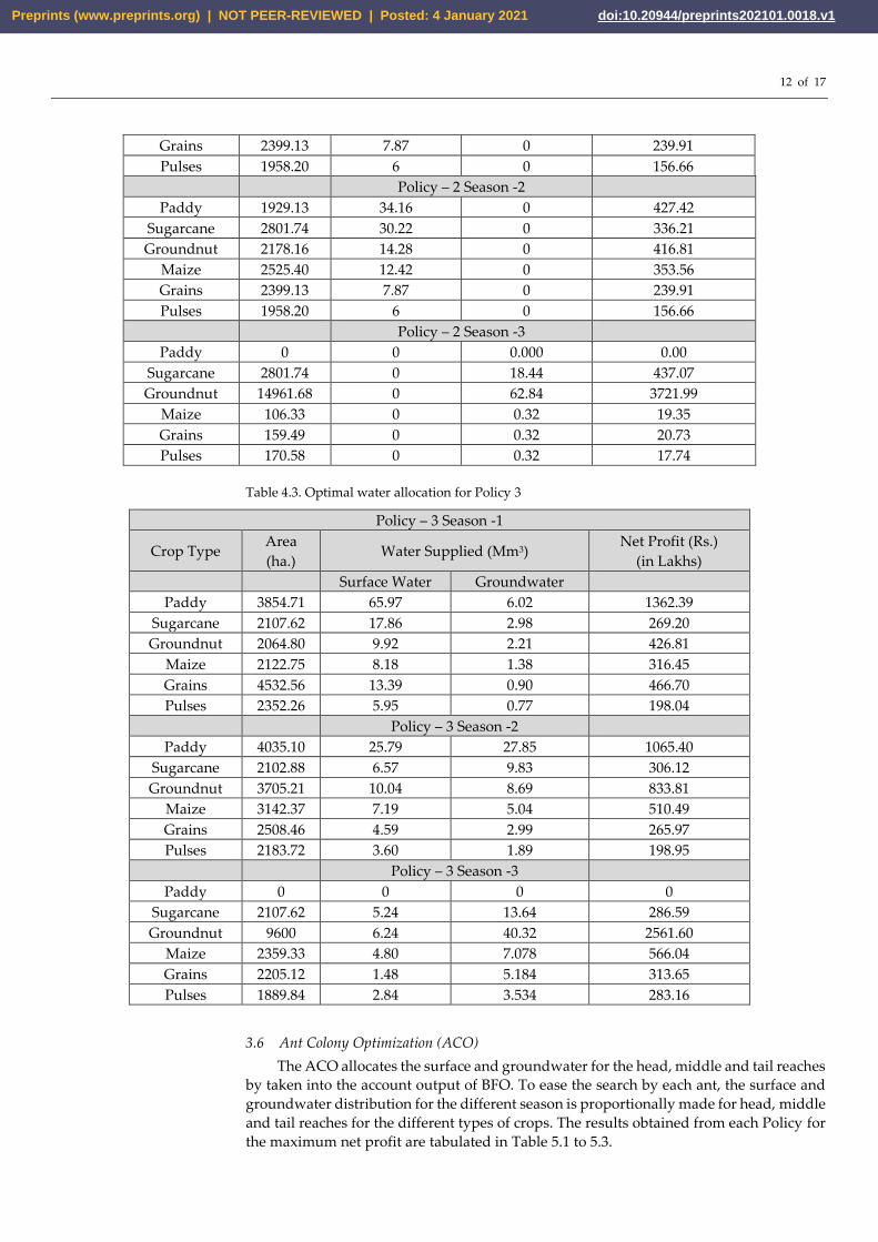
12 of 17

Grains 2399.13 7.87 0 239.91

Pulses 1958.20 6 0 156.66


Paddy 1929.13 34.16 0 427.42

Sugarcane 2801.74 30.22 0 336.21

Groundnut 2178.16 14.28 0 416.81

Maize 2525.40 12.42 0 353.56

Grains 2399.13 7.87 0 239.91

Pulses 1958.20 6 0 156.66


Paddy 0 0 0.000 0.00

Sugarcane 2801.74 0 18.44 437.07

Groundnut 14961.68 0 62.84 3721.99

Maize 106.33 0 0.32 19.35

Grains 159.49 0 0.32 20.73

Pulses 170.58 0 0.32 17.74



Crop Type Area

(ha.) Water Supplied (Mm3)

Net Profit (Rs.)

(in Lakhs)


Paddy 3854.71 65.97 6.02 1362.39

Sugarcane 2107.62 17.86 2.98 269.20

Groundnut 2064.80 9.92 2.21 426.81

Maize 2122.75 8.18 1.38 316.45

Grains 4532.56 13.39 0.90 466.70

Pulses 2352.26 5.95 0.77 198.04


Paddy 4035.10 25.79 27.85 1065.40

Sugarcane 2102.88 6.57 9.83 306.12

Groundnut 3705.21 10.04 8.69 833.81

Maize 3142.37 7.19 5.04 510.49

Grains 2508.46 4.59 2.99 265.97

Pulses 2183.72 3.60 1.89 198.95


Paddy 0 0 0 0

Sugarcane 2107.62 5.24 13.64 286.59

Groundnut 9600 6.24 40.32 2561.60

Maize 2359.33 4.80 7.078 566.04

Grains 2205.12 1.48 5.184 313.65

Pulses 1889.84 2.84 3.534 283.16

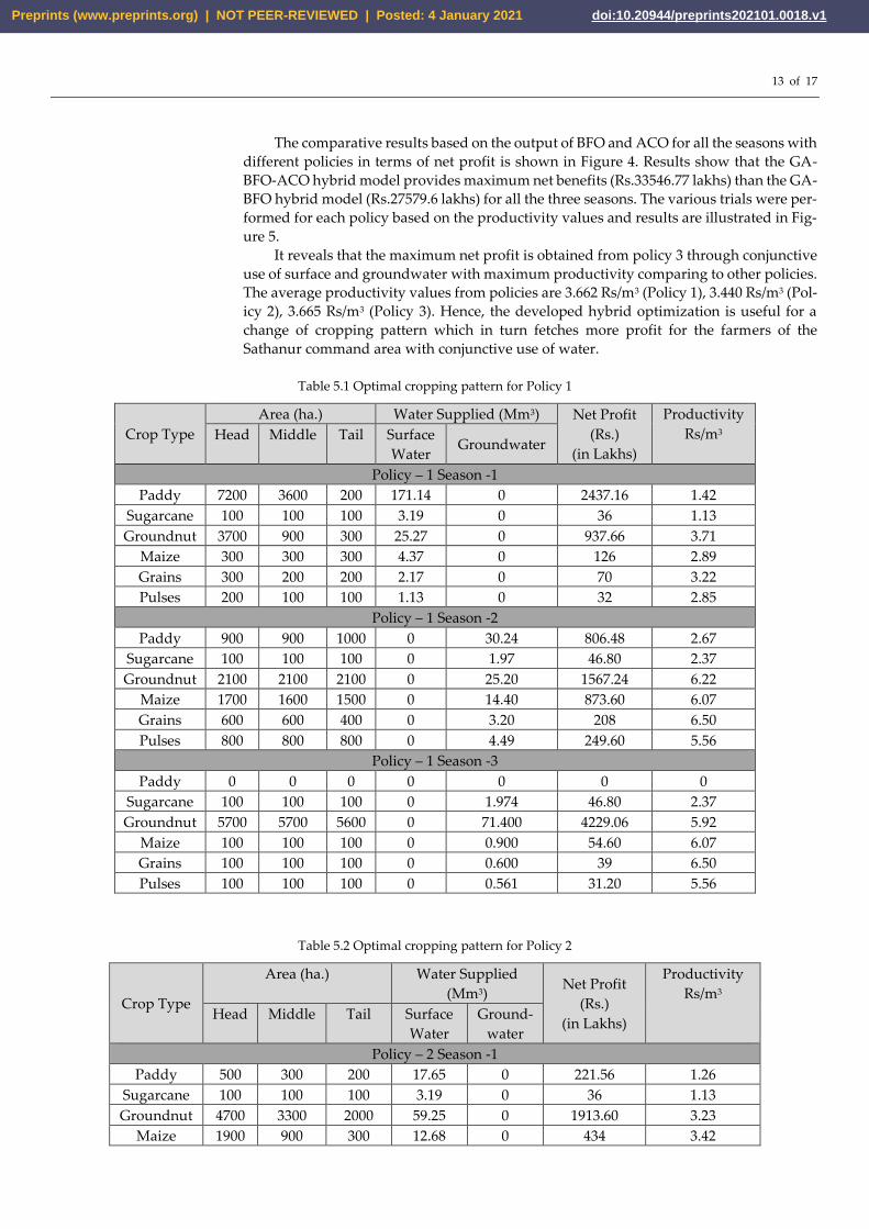
3.6 Ant Colony Optimization (ACO)

The ACO allocates the surface and groundwater for the head, middle and tail reaches

by taken into the account output of BFO. To ease the search by each ant, the surface and

groundwater distribution for the different season is proportionally made for head, middle

and tail reaches for the different types of crops. The results obtained from each Policy for

the maximum net profit are tabulated in Table 5.1 to 5.3.



13 of 17

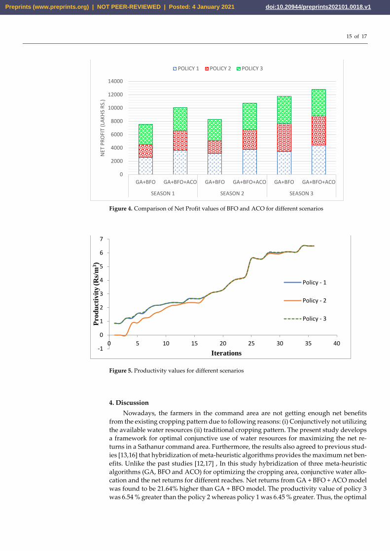
The comparative results based on the output of BFO and ACO for all the seasons with

different policies in terms of net profit is shown in Figure 4. Results show that the GA-

BFO-ACO hybrid model provides maximum net benefits (Rs.33546.77 lakhs) than the GA-

BFO hybrid model (Rs.27579.6 lakhs) for all the three seasons. The various trials were per-

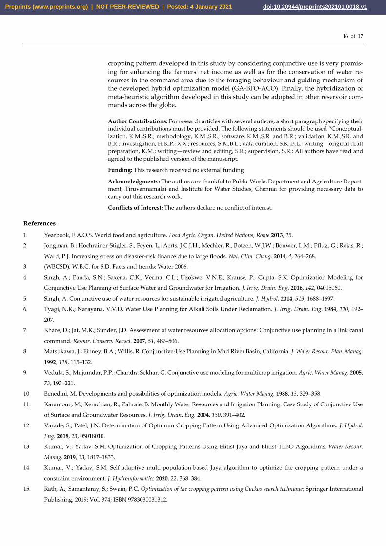
formed for each policy based on the productivity values and results are illustrated in Fig-

ure 5.

It reveals that the maximum net profit is obtained from policy 3 through conjunctive

use of surface and groundwater with maximum productivity comparing to other policies.

The average productivity values from policies are 3.662 Rs/m3 (Policy 1), 3.440 Rs/m3 (Pol-

icy 2), 3.665 Rs/m3 (Policy 3). Hence, the developed hybrid optimization is useful for a

change of cropping pattern which in turn fetches more profit for the farmers of the

Sathanur command area with conjunctive use of water.

Table 5.1 Optimal cropping pattern for Policy 1

Crop Type

Area (ha.) Water Supplied (Mm3) Net Profit

(Rs.)

(in Lakhs)

Productivity

Rs/m3 Head Middle Tail Surface

Water Groundwater


Paddy 7200 3600 200 171.14 0 2437.16 1.42

Sugarcane 100 100 100 3.19 0 36 1.13

Groundnut 3700 900 300 25.27 0 937.66 3.71

Maize 300 300 300 4.37 0 126 2.89

Grains 300 200 200 2.17 0 70 3.22

Pulses 200 100 100 1.13 0 32 2.85


Paddy 900 900 1000 0 30.24 806.48 2.67

Sugarcane 100 100 100 0 1.97 46.80 2.37

Groundnut 2100 2100 2100 0 25.20 1567.24 6.22

Maize 1700 1600 1500 0 14.40 873.60 6.07

Grains 600 600 400 0 3.20 208 6.50

Pulses 800 800 800 0 4.49 249.60 5.56


Paddy 0 0 0 0 0 0 0

Sugarcane 100 100 100 0 1.974 46.80 2.37

Groundnut 5700 5700 5600 0 71.400 4229.06 5.92

Maize 100 100 100 0 0.900 54.60 6.07

Grains 100 100 100 0 0.600 39 6.50

Pulses 100 100 100 0 0.561 31.20 5.56


Crop Type

Area (ha.) Water Supplied

(Mm3) Net Profit

(Rs.)

(in Lakhs)

Productivity

Rs/m3

Head Middle Tail Surface

Water

Ground-

water


Paddy 500 300 200 17.65 0 221.56 1.26

Sugarcane 100 100 100 3.19 0 36 1.13

Groundnut 4700 3300 2000 59.25 0 1913.60 3.23

Maize 1900 900 300 12.68 0 434 3.42



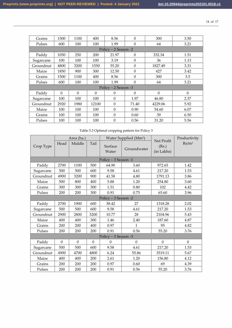
14 of 17

Grains 1500 1100 400 8.56 0 300 3.50

Pulses 600 100 100 1.99 0 64 3.21


Paddy 1050 250 200 21.97 0 332.34 1.51

Sugarcane 100 100 100 3.19 0 36 1.13

Groundnut 4800 3200 1550 55.20 0 1827.49 3.31

Maize 1850 900 300 12.50 0 427 3.42

Grains 1500 1100 400 8.56 0 300 3.5

Pulses 600 100 100 1.99 0 64 3.21


Paddy 0 0 0 0 0 0 0

Sugarcane 100 100 100 0 1.97 46.80 2.37

Groundnut 2920 1980 12100 0 71.40 4229.06 5.92

Maize 100 100 100 0 0.90 54.60 6.07

Grains 100 100 100 0 0.60 39 6.50

Pulses 100 100 100 0 0.56 31.20 5.56


Crop Type

Area (ha.) Water Supplied (Mm3) Net Profit

(Rs.)

(in Lakhs)

Productivity

Rs/m3 Head Middle Tail Surface

Water Groundwater


Paddy 2700 1100 500 64.90 3.60 972.65 1.42

Sugarcane 500 500 600 9.58 4.61 217.20 1.53

Groundnut 4900 3200 900 41.58 4.80 1791.13 3.86

Maize 500 800 400 5.88 1.20 254.80 3.60

Grains 300 300 300 1.51 0.80 102 4.42

Pulses 200 200 300 0.91 0.75 65.60 3.96


Paddy 2700 1900 600 38.42 27 1318.28 2.02

Sugarcane 500 500 600 9.58 4.61 217.20 1.53

Groundnut 2900 2800 3200 10.77 28 2104.96 5.43

Maize 400 400 300 1.46 2.40 187.60 4.87

Grains 200 200 400 0.97 1 95 4.82

Pulses 200 200 200 0.91 0.56 55.20 3.76


Paddy 0 0 0 0 0 0 0

Sugarcane 500 500 600 9.58 4.61 217.20 1.53

Groundnut 4900 4700 4800 6.24 55.86 3519.11 5.67

Maize 400 400 200 2.61 1.20 156.80 4.12

Grains 200 200 200 0.97 0.60 69 4.39

Pulses 200 200 200 0.91 0.56 55.20 3.76



15 of 17

Figure 4. Comparison of Net Profit values of BFO and ACO for different scenarios

Figure 5. Productivity values for different scenarios

4. Discussion

Nowadays, the farmers in the command area are not getting enough net benefits

from the existing cropping pattern due to following reasons: (i) Conjunctively not utilizing

the available water resources (ii) traditional cropping pattern. The present study develops

a framework for optimal conjunctive use of water resources for maximizing the net re-

turns in a Sathanur command area. Furthermore, the results also agreed to previous stud-

ies [13,16] that hybridization of meta-heuristic algorithms provides the maximum net ben-

efits. Unlike the past studies [12,17] , In this study hybridization of three meta-heuristic

algorithms (GA, BFO and ACO) for optimizing the cropping area, conjunctive water allo-

cation and the net returns for different reaches. Net returns from GA + BFO + ACO model

was found to be 21.64% higher than GA + BFO model. The productivity value of policy 3

was 6.54 % greater than the policy 2 whereas policy 1 was 6.45 % greater. Thus, the optimal

0

2000

4000

6000

8000

10000

12000

14000

GA+BFO GA+BFO+ACO GA+BFO GA+BFO+ACO GA+BFO GA+BFO+ACO

SEASON 1 SEASON 2 SEASON 3

NET

PR

OFI

T (L

AK

HS

RS.

)

POLICY 1 POLICY 2 POLICY 3

-1

0

1

2

3

4

5

6

7

0 5 10 15 20 25 30 35 40

Pro

du

ctiv

ity

(Rs/

m3)

Iterations

Policy - 1

Policy - 2

Policy - 3



16 of 17

cropping pattern developed in this study by considering conjunctive use is very promis-

ing for enhancing the farmers' net income as well as for the conservation of water re-

sources in the command area due to the foraging behaviour and guiding mechanism of

the developed hybrid optimization model (GA-BFO-ACO). Finally, the hybridization of

meta-heuristic algorithm developed in this study can be adopted in other reservoir com-

mands across the globe.

Author Contributions: For research articles with several authors, a short paragraph specifying their

individual contributions must be provided. The following statements should be used “Conceptual-

ization, K.M.,S.R.; methodology, K.M.,S.R.; software, K.M.,S.R. and B.R.; validation, K.M.,S.R. and

B.R.; investigation, H.R.P.; X.X.; resources, S.K.,B.L.; data curation, S.K.,B.L.; writing—original draft

preparation, K.M.; writing—review and editing, S.R.; supervision, S.R.; All authors have read and

agreed to the published version of the manuscript.

Funding: This research received no external funding

Acknowledgments: The authors are thankful to Public Works Department and Agriculture Depart-

ment, Tiruvannamalai and Institute for Water Studies, Chennai for providing necessary data to

carry out this research work.

Conflicts of Interest: The authors declare no conflict of interest.

References

1. Yearbook, F.A.O.S. World food and agriculture. Food Agric. Organ. United Nations, Rome 2013, 15.

2. Jongman, B.; Hochrainer-Stigler, S.; Feyen, L.; Aerts, J.C.J.H.; Mechler, R.; Botzen, W.J.W.; Bouwer, L.M.; Pflug, G.; Rojas, R.;

Ward, P.J. Increasing stress on disaster-risk finance due to large floods. Nat. Clim. Chang. 2014, 4, 264–268.

3. (WBCSD), W.B.C. for S.D. Facts and trends: Water 2006.

4. Singh, A.; Panda, S.N.; Saxena, C.K.; Verma, C.L.; Uzokwe, V.N.E.; Krause, P.; Gupta, S.K. Optimization Modeling for

Conjunctive Use Planning of Surface Water and Groundwater for Irrigation. J. Irrig. Drain. Eng. 2016, 142, 04015060.

5. Singh, A. Conjunctive use of water resources for sustainable irrigated agriculture. J. Hydrol. 2014, 519, 1688–1697.

6. Tyagi, N.K.; Narayana, V.V.D. Water Use Planning for Alkali Soils Under Reclamation. J. Irrig. Drain. Eng. 1984, 110, 192–

207.

7. Khare, D.; Jat, M.K.; Sunder, J.D. Assessment of water resources allocation options: Conjunctive use planning in a link canal

command. Resour. Conserv. Recycl. 2007, 51, 487–506.

8. Matsukawa, J.; Finney, B.A.; Willis, R. Conjunctive-Use Planning in Mad River Basin, California. J. Water Resour. Plan. Manag.

1992, 118, 115–132.

9. Vedula, S.; Mujumdar, P.P.; Chandra Sekhar, G. Conjunctive use modeling for multicrop irrigation. Agric. Water Manag. 2005,

73, 193–221.

10. Benedini, M. Developments and possibilities of optimization models. Agric. Water Manag. 1988, 13, 329–358.

11. Karamouz, M.; Kerachian, R.; Zahraie, B. Monthly Water Resources and Irrigation Planning: Case Study of Conjunctive Use

of Surface and Groundwater Resources. J. Irrig. Drain. Eng. 2004, 130, 391–402.

12. Varade, S.; Patel, J.N. Determination of Optimum Cropping Pattern Using Advanced Optimization Algorithms. J. Hydrol.

Eng. 2018, 23, 05018010.

13. Kumar, V.; Yadav, S.M. Optimization of Cropping Patterns Using Elitist-Jaya and Elitist-TLBO Algorithms. Water Resour.

Manag. 2019, 33, 1817–1833.

14. Kumar, V.; Yadav, S.M. Self-adaptive multi-population-based Jaya algorithm to optimize the cropping pattern under a

constraint environment. J. Hydroinformatics 2020, 22, 368–384.

15. Rath, A.; Samantaray, S.; Swain, P.C. Optimization of the cropping pattern using Cuckoo search technique; Springer International

Publishing, 2019; Vol. 374; ISBN 9783030031312.



17 of 17

16. Rath, A.; Swain, P.C. Optimal allocation of agricultural land for crop planning in Hirakud canal command area using swarm

intelligence techniques. ISH J. Hydraul. Eng. 2018, 1–13.

17. Mohammadrezapour, O.; Yoosefdoost, I.; Ebrahimi, M. Cuckoo optimization algorithm in optimal water allocation and crop

planning under various weather conditions (case study: Qazvin plain, Iran). Neural Comput. Appl. 2019, 31, 1879–1892.

18. Safavi, H.R.; Falsafioun, M. Conjunctive use of surface water and groundwater resources under deficit irrigation. J. Irrig.

Drain. Eng. 2017, 143, 1–9.

19. Kannan, M.G.V. Paddy Yield Estimation Using Remote Sensing and Geographical Information System. J. Mod. Biotechnol.

2012, 1, 26–30.

20. Allen, Richard G and Pereira, Luis S and Raes, Dirk and Smith, M. and others Crop evapotranspiration-Guidelines for

computing crop water requirements-FAO Irrigation and drainage paper 56. Fao, Rome 1988, 300, D05109.

21. Jensen, M.E.; Burman, R.D.; Allen, R.G. Evapotranspiration and irrigation water requirements.; ASCE, 1990.

22. Smajstrla, Allen George and Zazueta, F. Estimating crop irrigation requirements for irrigation system design and consumptive use

permitting; University of Florida Cooperative Extension Service, Institute of Food and Agriculture Sciences, EDIS., 1998;

23. Smith, M. CROPWAT: A computer program for irrigation planning and management; 46th ed.; Food \& Agriculture Org, 1992;

24. Islam, S.; Talukdar, B. Crop yield optimization using genetic algorithm with the CROPWAT model as a decision support

system. Int. J. Agric. Eng. 2014, 7, 7–14.

25. USDA, S. National Engineering Handbook, Sec. 4 Hydrology. Washingt. DC 1964.

26. Mishra, S.K.; Singh, V.P. SCS-CN Method. In Soil Conservation Service Curve Number (SCS-CN) Methodology; Springer

Netherlands: Dordrecht, 2003; pp. 84–146 ISBN 978-94-017-0147-1.

27. Methodology, G.R.E. Report of the groundwater resource estimation committee. Minist. Water Resour. Gov. India, New Delhi

1997, 107.

28. Scanlon, B.R.; Healy, R.W.; Cook, P.G. Choosing appropriate techniques for quantifying groundwater recharge. Hydrogeol. J.

2002, 10, 18–39.

29. Holland, J.H. Adaptation in Natural and Artificial Systems; MIT Press: Cambridge, MA, USA, 1992; ISBN 0-262-58111-6.

30. Whitley, D. A genetic algorithm tutorial. Stat. Comput. 1994, 4, 65–85.

31. Dobslaw, F. A parameter-tuning framework for metaheuristics based on design of experiments and artificial neural networks.

World Acad. Sci. Eng. Technol. 2010, 64, 213–216.

32. Sahoo, B.; Walling, I.; Deka, B.C.; Bhatt, B.P. Standardization of reference evapotranspiration models for a subhumid valley

rangeland in the Eastern Himalayas. J. Irrig. Drain. Eng. 2012, 138, 880–895.

33. Ghosh, A.; Dehuri, S. Evolutionary Algorithms for Multi-Criterion Optimization: A Survey. Int. J. Comput. Inf. Sci. 2004, 2,

38–57.

34. Passino, K.M. Biomimicry of bacterial foraging for distributed optimization and control. IEEE Control Syst. Mag. 2002, 22, 52–

67.

35. Meuleau, N.; Dorigo, M. Ant colony optimization and stochastic gradient descent. Artif. Life 2002, 8, 103–121.



Documents

Hybrid optimization model for conjunctive use of surface