Embed Size (px)
Citation preview
Western Michigan University Western Michigan University
ScholarWorks at WMU ScholarWorks at WMU
Dissertations Graduate College
6-2018
Hybrid Model - Statistical Features and Deep Neural Network for Hybrid Model - Statistical Features and Deep Neural Network for
Brain Tumor Classification in MRI Images Brain Tumor Classification in MRI Images
Mustafa Rashid Ismael Western Michigan University, [email protected]
Follow this and additional works at: https://scholarworks.wmich.edu/dissertations
Part of the Analytical, Diagnostic and Therapeutic Techniques and Equipment Commons
Recommended Citation Recommended Citation Ismael, Mustafa Rashid, "Hybrid Model - Statistical Features and Deep Neural Network for Brain Tumor Classification in MRI Images" (2018). Dissertations. 3291. https://scholarworks.wmich.edu/dissertations/3291
This Dissertation-Open Access is brought to you for free and open access by the Graduate College at ScholarWorks at WMU. It has been accepted for inclusion in Dissertations by an authorized administrator of ScholarWorks at WMU. For more information, please contact [email protected].

HYBRID MODEL - STATISTICAL FEATURES AND DEEP NEURAL NETWORK
FOR BRAIN TUMOR CLASSIFICATION IN MRI IMAGES
by
Mustafa Rashid Ismael
A dissertation submitted to the Graduate College
in partial fulfillment of the requirements
for the degree of Doctor of Philosophy
Electrical and Computer Engineering
Western Michigan University
June 2018
Doctoral Committee:
Ikhlas Abdel-Qader, Ph.D., Chair
Janos L. Grantner, Ph.D.
Azim Houshyar, Ph.D.

Copyright by
Mustafa Rashid Ismael
2018

HYBRID MODEL - STATISTICAL FEATURES AND DEEP NEURAL NETWORK
FOR BRAIN TUMOR CLASSIFICATION IN MRI IMAGES
Mustafa Rashid Ismael, Ph.D.
Western Michigan University, 2018
A brain tumor is the most common disease that affects the central nervous system (CNS),
the brain, and spinal cord. It can be diagnosed using the safest and most reliable imaging modality,
the Magnetic Resonance Imaging (MRI), by radiologists who may use the assistance of computer-
aided diagnosis (CAD) tools. Automated diagnosis is sought because it is essential to overcome
the drawbacks of the manual diagnosis, such as time and the stress of viewing MRI images for
long hours, and the human error potential. Image analysis and machine learning algorithms are
tools that can be used to build an intelligent CAD system capable of analyzing brain tumors and
formulating a diagnosis on its own. Hence, it is essential to design a CAD system that is capable
of extracting meaningful and precise information, and rendering an error-free diagnosis.
Consequently, many researchers have proposed different methods to develop a CAD system to
detect and classify abnormal growths in brain images.
This dissertation presents a hybrid system for tumor classification from brain MRI images.
The hybrid system is composed of a set of statistical-based features and deep neural networks.
Segments of the MRI, from within the region of interest (ROI), are transformed into the two-
dimensional Discrete Wavelet Transform and the two-dimensional Gabor filter methods. This
allows the set of features to encompass all the directional information of the spatial domain tumor
characteristics. A classifier system is developed using two types of neural network algorithms,
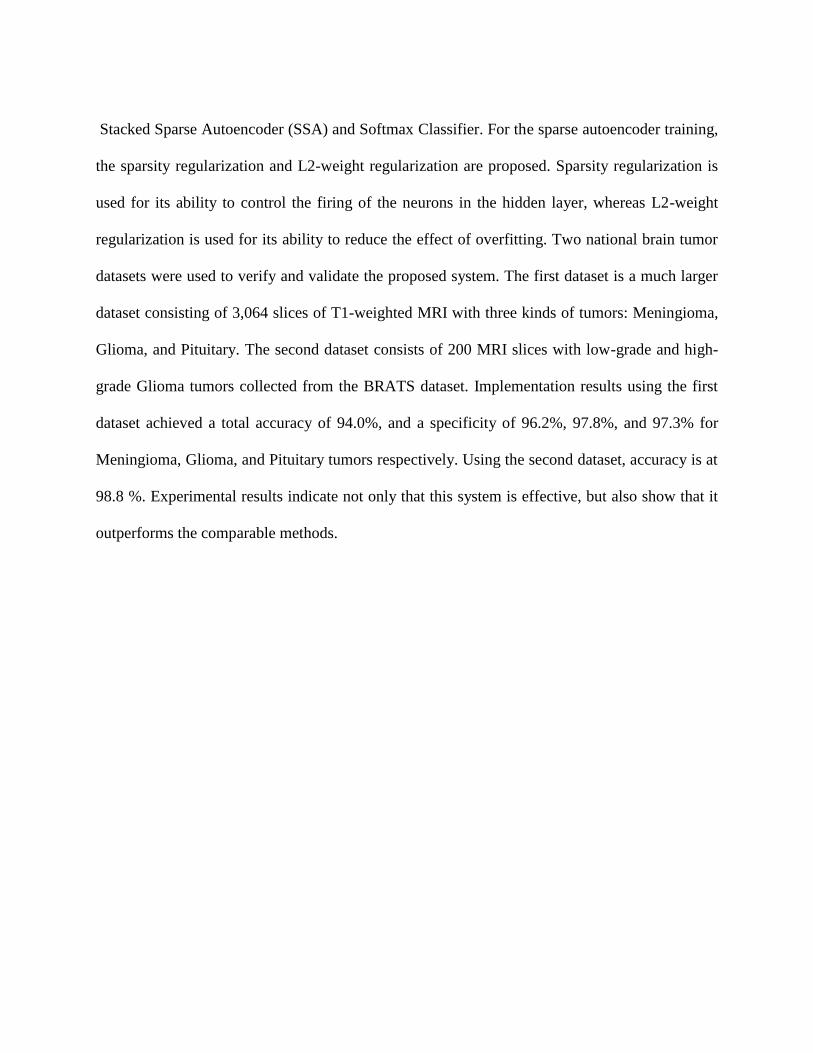
Stacked Sparse Autoencoder (SSA) and Softmax Classifier. For the sparse autoencoder training,
the sparsity regularization and L2-weight regularization are proposed. Sparsity regularization is
used for its ability to control the firing of the neurons in the hidden layer, whereas L2-weight
regularization is used for its ability to reduce the effect of overfitting. Two national brain tumor
datasets were used to verify and validate the proposed system. The first dataset is a much larger
dataset consisting of 3,064 slices of T1-weighted MRI with three kinds of tumors: Meningioma,
Glioma, and Pituitary. The second dataset consists of 200 MRI slices with low-grade and high-
grade Glioma tumors collected from the BRATS dataset. Implementation results using the first
dataset achieved a total accuracy of 94.0%, and a specificity of 96.2%, 97.8%, and 97.3% for
Meningioma, Glioma, and Pituitary tumors respectively. Using the second dataset, accuracy is at
98.8 %. Experimental results indicate not only that this system is effective, but also show that it
outperforms the comparable methods.

ii
ACKNOWLEDGMENTS
My heartfelt gratitude and thanks must be first offered to God for his merciful support and
guidance to complete this work.
I would like to express my deep appreciation and gratitude to my supervisor “Prof. Dr.
Ikhlas Abdel-Qader” for her invaluable guidance, encouragement, and advice that she generously
gave me throughout this work. Without her scientific and technical assistance, the dissertation
would never have been completed. Also, I would like to extend my sincere gratitude to my
committee members: Dr. Janos L. Grantner, Dr. Azim Houshyar, for their support and supervision
during this dissertation process.
Special thanks to my father and mother, without their support and prayers, I could not be
where I am now. I am ever grateful for their love and trust in my judgment, which opened the door
to my education.
Finally, I would like to thank my wife for her patience and support during all the years of
my study. She always encourages me to work harder and accomplish my academic degree. Thus,
I am dedicating this dissertation to my parents, my wife, and my lovely daughter “Razan”.
Mustafa Rashid Ismael
iii
TABLE OF CONTENTS
ACKNOWLEDGMENTS .............................................................................................................. ii
LIST OF TABLES ......................................................................................................................... vi
LIST OF FIGURES ..................................................................................................................... viii
CHAPTER
I. INTRODUCTION .............................................................................................................. 1
1.1 Problem Statement ...................................................................................................... 1
1.2 Significance ................................................................................................................. 2
1.3 Background ................................................................................................................. 3
1.3.1 Brain Tumors .................................................................................................. 3
1.3.2 Magnetic Resonance Imaging ......................................................................... 5
1.3.3 Computer-aided Diagnosis System for Brain Tumor Analysis ...................... 8
1.4 The Aim of the Research ........................................................................................... 11
1.5 Organization of the Dissertation ................................................................................ 12
II. RELATED WORKS ......................................................................................................... 13
2.1 Introduction ............................................................................................................... 13
2.2 Classification Approach ............................................................................................ 14
2.3 Database .................................................................................................................... 15
2.4 Methodology ............................................................................................................. 16
2.4.1 Image Preprocessing ..................................................................................... 16
2.4.2 Image Segmentation ...................................................................................... 17
2.4.3 Feature Extraction ......................................................................................... 18
2.4.4 Dimensionality Reduction ............................................................................ 20
iv
Table of Contents-Continued
CHAPTER
2.4.5 Classification Techniques ............................................................................. 21
III. THE PROPOSED FRAMEWORK: BRAIN TUMOR CLASSIFICATION USING A
HYBRID DOMAIN BASED STATISTICAL FEATURES ............................................ 27
3.1 Introduction ............................................................................................................... 27
3.2 The Framework of The Proposed System ................................................................. 29
3.3 Feature Extraction ..................................................................................................... 31
3.3.1 Discrete Wavelet Transform ......................................................................... 31
3.3.2 Gabor Filter ................................................................................................... 36
3.3.3 Statistical Features ........................................................................................ 39
3.3.4 The Proposed Method for Feature Extraction ............................................... 45
3.4 Classification using Stacked Sparse Autoencoder and Softmax Classifier ............... 47
3.4.1 Introduction to Neural Network .................................................................... 47
3.4.2 Training Using Backpropagation Algorithm ................................................ 50
3.4.3 Autoencoder .................................................................................................. 55
3.4.4 Sparse Autoencoder ...................................................................................... 57
3.4.5 Stacked Sparse Autoencoder ......................................................................... 60
3.4.6 Softmax Classifier ......................................................................................... 60
3.4.7 Training the Stacked Sparse Autoencoder and the Softmax Layer .............. 61
IV. EXPERIMENTAL SETUP AND RESULTS ................................................................... 65
4.1 Database .................................................................................................................... 65
4.2 Experimental Setup ................................................................................................... 66
v
Table of Contents-Continued
CHAPTER
4.3 Performance Analysis ................................................................................................ 70
4.4 Simulation Results ..................................................................................................... 72
4.4.1 Statistical Features Obtained from Wavelet Transform and Gabor Filter .... 72
4.4.2 Confusion Matrix .......................................................................................... 75
4.4.3 Wavelet Features ........................................................................................... 78
4.4.4 Gabor Features .............................................................................................. 81
4.4.5 Gabor Filter vs Wavelet Transform .............................................................. 82
4.4.6 The Effect of Sparsity Regularization and L2-weight Regularization
Coefficients on the Performance of the Algorithm ....................................... 84
4.4.7 Classification Using Neural Network ........................................................... 90
4.4.8 Comparison with Related Works .................................................................. 96
4.5 Implementation and Time Processing ....................................................................... 98
V. CONCLUSIONS AND FUTURE WORK ..................................................................... 100
5.1 Summary ................................................................................................................. 100
5.2 Contribution ............................................................................................................. 102
5.3 Future Works ........................................................................................................... 102
BIBLIOGRAPHY ....................................................................................................................... 103

vi
LIST OF TABLES
3.1: Tumor types/grades descriptions ........................................................................................... 27
4.1: Statistical features obtained from the third level of Wavelet Transform ............................... 73
4.2: Statistical features obtained from Gabor filter with wavelength λ orientation 90° ............... 74
4.3: Confusion matrix for the first database.................................................................................. 75
4.4: Confusion matrix for the BRATS database ........................................................................... 76
4.5: True positive, true negative, false positive, and false negative rates ..................................... 77
4.6: Accuracy, sensitivity, and specificity for the three types of tumors ...................................... 77
4.7: Performance analysis of the proposed method for the first dataset using the wavelet
features ................................................................................................................................... 80
4.8: Performance analysis of the proposed method for the BRATS dataset using the wavelet
features ................................................................................................................................... 80
4.9: Performance analysis of the proposed algorithm for the BRATS dataset with Gabor and
Gabor energy features ............................................................................................................ 82
4.10: Performance analysis of the proposed algorithm for the first dataset with Gabor and
Gabor energy features .......................................................................................................... 81
4.11: Comparison the performance of the proposed algorithm for the First dataset with
wavelet features, Gabor features, and combined features ................................................... 83
4.12: Comparison the performance of the proposed algorithm for the BRATS dataset with
wavelet features, Gabor features, and combined features ................................................... 83
4.13: Confusion matrix for the first database (Neural Network Classifier) .................................. 91
4.14: Confusion matrix for the BRATS database (Neural Network Classifier) ........................... 91
4.15: Comparison the performance of the proposed algorithm with neural network classifier
for the first dataset ............................................................................................................... 94

vii
List of Tables-Continued
4.16: Comparison the performance of the proposed algorithm with neural network classifier
for the first dataset ............................................................................................................... 95
4.17: Comparison with related work (first dataset) ...................................................................... 96
4.18: Comparison with related work (BRATS dataset) ................................................................ 97
4.19: Processing time for training and testing phase .................................................................... 98

viii
LIST OF FIGURES
2.1: General CAD system for brain tumor analysis ...................................................................... 13
3.1: MRI sample images showing the three types of tumors and the two grades of Glioma
Tumor .................................................................................................................................... 28
3.2: Block diagram of the proposed algorithm ............................................................................. 30
3.3: Two-channel, three-level analysis filter bank with 1-D DWT .............................................. 34
3.4: One level filter bank for computation of 2-D DWT .............................................................. 35
3.5: Image Decomposition using 2-levels of 2-D DWT ............................................................... 36
3.6: Gabor filter shape with different wavelengths and orientations, (a) 𝜆 = 2, 𝜃 = 0°, (b)
𝜆 = 2, 𝜃 = 90°, (c) 𝜆 = 4, 𝜃 = 0°, and (d) 𝜆 = 4, 𝜃 = 90°............................................... 38
3.7: Gabor filter shape with the symmetric and antisymmetric kernel, (a) 𝜆 = 4, 𝜃 = 90°, 𝜓 = 0°, (b) 𝜆 = 4, 𝜃 = 90°, 𝜓 = 90° .................................................................................. 39
3.8: Example of image histogram, (a) an image, (b) its histogram ............................................... 40
3.9: Example of GLCM matrix generation, (a) an image, (b) its GLCM matrix .......................... 42
3.10: A Nonlinear model of a neuron ........................................................................................... 47
3.11: Threshold function ............................................................................................................... 48
3.12: Sigmoid function.................................................................................................................. 49
3.13: Architecture of multilayer neural network ........................................................................... 50
3.14: Basic architecture of Autoencoder ....................................................................................... 55
3.15: Architecture of four layers Stacked Sparse Autoencoder .................................................... 60
3.16: Architecture of Softmax classifier ....................................................................................... 61
3.17: An example of stacked sparse autoencoder and Softmax layer classifier ........................... 64
4.1: Sample images from the first database, (a) Meningioma, (b) Glioma, and (c) Pituitary and
its tumor mask (d), (e), and (f) respectively .......................................................................... 66
ix
List of Figures-Continued
4.2: Sample images from BRATS database, (a) High-grade Glioma, (b) Low-grade Glioma,
and its tumor mask (c), and (d) respectively .......................................................................... 67
4.3: Image decomposition using three levels of 2-D DWT, the input image is MRI with
Meningioma tumor. ............................................................................................................... 68
4.4: Visualization of images resulted from 2-D Gabor filter with three values of wavelengths
and five values of orientations, (a) the original image, (b) its tumor mask, numbers in
brackets are (wavelength, orientation) ................................................................................... 69
4.5: ROC Curve for the classification model, (a) first dataset, (b) BRATS dataset ..................... 78
4.6: Classification accuracies for different types of wavelet filters .............................................. 79
4.7: The effect of sparsity regularization coefficient on the system accuracy .............................. 85
4.8: The effect of L2-wight regularization coefficient on the system accuracy ........................... 85
4.9: Autoencoder training performance for the first dataset, (a) first autoencoder, (b) second
autoencoder ............................................................................................................................ 87
4.10: View of the proposed classifier network ............................................................................. 86
4.11: Performance of the classifier network for the first dataset after stacking the sparse
autoencoder with the Softmax classifier .............................................................................. 88
4.12: Autoencoder training performance for the second dataset, (a) first autoencoder, (b)
second autoencoder.............................................................................................................. 89
4.13: Performance of the classifier network for the second dataset after stacking the sparse
autoencoder with the Softmax classifier .............................................................................. 90
4.14: Architecture of neural network classifier ............................................................................. 91
4.15: ROC Curve for the Neural Network Classifier, (a) first dataset, (b) BRATS dataset ......... 92
4.16: View of the neural network classifier ................................................................................ 922
4.17: Performance of the neural network classifier (a) for the first dataset, (b) for the second
dataset ................................................................................................................................ 933

1
CHAPTER I
1.INTRODUCTION
Brain tumors are the most common brain disease that affects the central nervous system
(CNS), the brain and the spinal cord [1]. According to the American cancer society, in 2018 CNS
tumors in both adults and children is estimated as “About 23,880 malignant tumors of the brain or
spinal cord (13,720 in males and 10,160 in females) will be diagnosed. These numbers would be
much higher if benign tumors were also included. About 16,830 people (9,490 males and 7,340
females) will die from brain and spinal cord tumors” [2]. Consequently; scientists in the field of
medicine, computer science, and engineering are working on developing new techniques to
diagnose and treat brain tumors effectively [1]. During the last two decades, the computer-aided
diagnosis system (CAD) has been employed to improve the accuracy of the diagnostic ability of
radiologists in detecting, segmenting, and identifying the type of brain tumor [3].
A brief introduction about brain tumor classification is presented in this chapter. First, the
problem of identifying the type and grade of tumor and why it is important is given in sections 1.1
and 1.2. Then, the basic idea of brain tumors, magnetic resonance imaging, and CAD are described
in section 1.3.
1.1 Problem Statement
To diagnose a patient with a brain tumor, radiologists use one of two techniques, invasive
or noninvasive. Noninvasive techniques are the most widely used one for this purpose and can be
implemented using medical imaging modalities like Computed Tomography (CT) scan, Magnetic
2
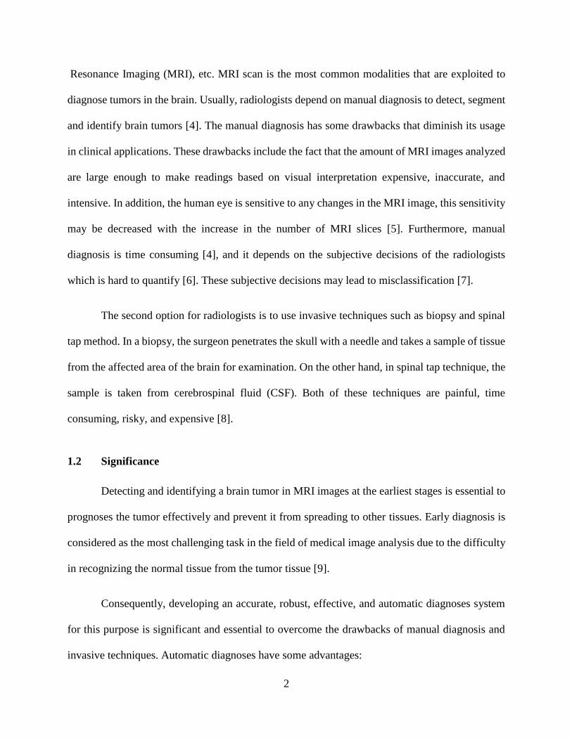
Resonance Imaging (MRI), etc. MRI scan is the most common modalities that are exploited to
diagnose tumors in the brain. Usually, radiologists depend on manual diagnosis to detect, segment
and identify brain tumors [4]. The manual diagnosis has some drawbacks that diminish its usage
in clinical applications. These drawbacks include the fact that the amount of MRI images analyzed
are large enough to make readings based on visual interpretation expensive, inaccurate, and
intensive. In addition, the human eye is sensitive to any changes in the MRI image, this sensitivity
may be decreased with the increase in the number of MRI slices [5]. Furthermore, manual
diagnosis is time consuming [4], and it depends on the subjective decisions of the radiologists
which is hard to quantify [6]. These subjective decisions may lead to misclassification [7].
The second option for radiologists is to use invasive techniques such as biopsy and spinal
tap method. In a biopsy, the surgeon penetrates the skull with a needle and takes a sample of tissue
from the affected area of the brain for examination. On the other hand, in spinal tap technique, the
sample is taken from cerebrospinal fluid (CSF). Both of these techniques are painful, time
consuming, risky, and expensive [8].
1.2 Significance
Detecting and identifying a brain tumor in MRI images at the earliest stages is essential to
prognoses the tumor effectively and prevent it from spreading to other tissues. Early diagnosis is
considered as the most challenging task in the field of medical image analysis due to the difficulty
in recognizing the normal tissue from the tumor tissue [9].
Consequently, developing an accurate, robust, effective, and automatic diagnoses system
for this purpose is significant and essential to overcome the drawbacks of manual diagnosis and
invasive techniques. Automatic diagnoses have some advantages:

3
1. It can help radiologists by providing a second opinion based on the information interpreted
from medical images [3].
2. Avoid human errors such as missing readings especially that is caused by fatigue,
overlooked, and data overloaded when analyzing a large amount of MRI slices [10].
1.3 Background
In this section, a brief background is presented focusing on brain tumors, magnetic
resonance imaging (MRI), and CAD for brain tumor analysis.
1.3.1 Brain Tumors
A brain tumor is defined as any abnormal tissue that grows in the central nervous system
(CNS) and prevents the brain from working properly. A brain tumor can be categorized according
to its aggressiveness as benign and malignant tumors. A benign brain tumor has no cancer cells
and grows slowly inside the brain with a clear border. Malignant brain tumors are more aggressive
than benign tumors, it has cancer cells with no clear border. This type of tumor can spread rapidly
and affect the surrounding brain tissues. In addition, a brain tumor can be divided into primary and
secondary depending on where the tumor cells began. Primary brain tumors originate from brain
cells and spread to other parts of the brain while secondary brain tumors originate from tissues
outside the brain and spread to the brain. Secondary brain tumors are more common than primary
and its treatment depends on the original tissue that the tumor starts from [11].
Some types of tumors are given a grade [1], this grade shows the growth speed of tumor
cells [11]. The grade ranges start from Grade I (the less malignant) to Grade IV (the most
malignant) [12]. Brain tumors can be treated using “surgery, radiation therapy, or chemotherapy”
depending on the type, grade, and size of the tumor [1]. According to the World Health

4
Organization (WHO), there are more than 120 types of brain and central nervous system tumors.
The most common types are [11]:
1.3.1.1 Glioma
A glioma tumor is the most widely diagnosed primary tumors in adults. It starts from the
glial cells in the brain and spread to the surrounding tissue [13]. This type of tumor appears as a
region with a heterogeneous texture region, a decreased signal intensity and a bright tumor border
[14]. It can be categorized according to its location and origin as:
i. Astrocytoma
This type of glioma tumor begins from cells called ‘astrocytes’. Typically, astrocytoma
tumor found in the cerebrum and it is subdivided into low grade (Grade I and Grade II) or high
grade (Grade III and Grade IV). Grade IV of astrocytoma is considered the most aggressive type
as compared to other brain tumors kinds and it is called ‘Glioblastoma’.
ii. Oligodendroglioma
Oligodendroglioma tumors are found in the cerebral hemispheres and begin from brain
cells with Grade I and Grade II distinction. The main side effects of this tumor are headaches,
seizures, sleepiness, and weakness.
1.3.1.2 Meningioma
Meningioma is a benign tumor that originates from the shell cover the brain and it is located
under the skull. In adults, this type of tumor is considered as one-third of brain tumors and typically
it grows slowly inside the brain [11]. Meningioma tumor appears as extra-axial masses with the
homogeneous region and increased signal intensity (brighter than the surrounding tissue) [15].
5
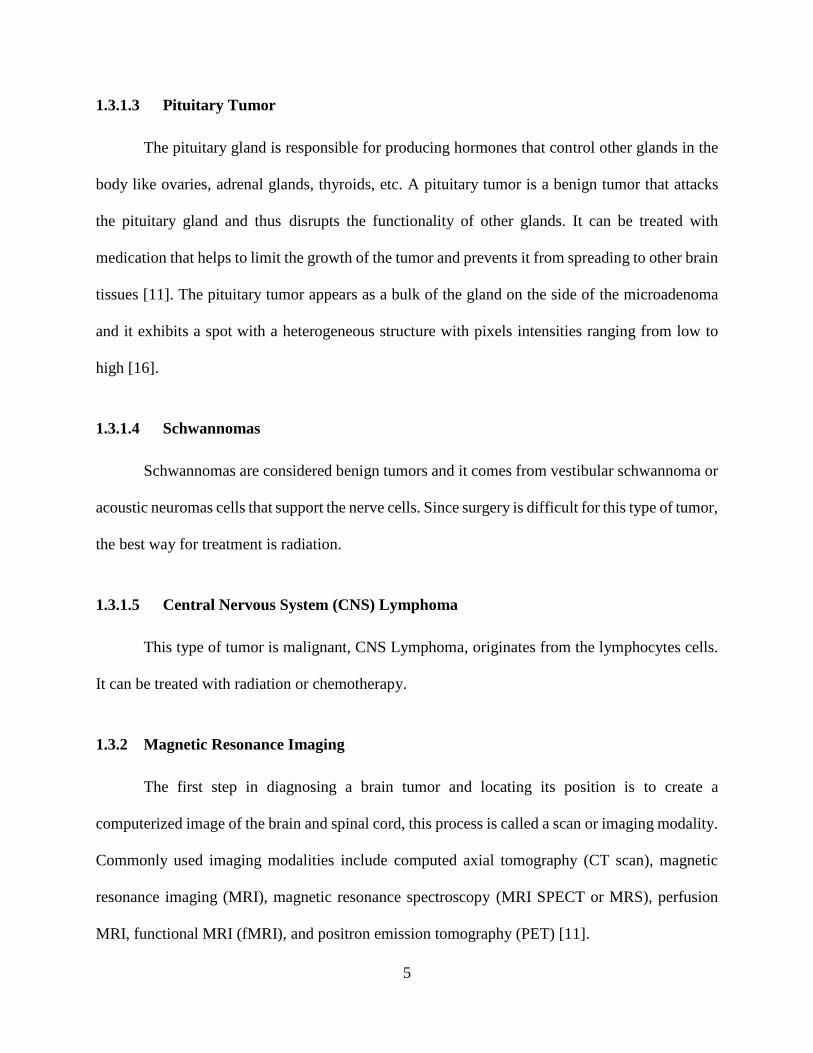
1.3.1.3 Pituitary Tumor
The pituitary gland is responsible for producing hormones that control other glands in the
body like ovaries, adrenal glands, thyroids, etc. A pituitary tumor is a benign tumor that attacks
the pituitary gland and thus disrupts the functionality of other glands. It can be treated with
medication that helps to limit the growth of the tumor and prevents it from spreading to other brain
tissues [11]. The pituitary tumor appears as a bulk of the gland on the side of the microadenoma
and it exhibits a spot with a heterogeneous structure with pixels intensities ranging from low to
high [16].
1.3.1.4 Schwannomas
Schwannomas are considered benign tumors and it comes from vestibular schwannoma or
acoustic neuromas cells that support the nerve cells. Since surgery is difficult for this type of tumor,
the best way for treatment is radiation.
1.3.1.5 Central Nervous System (CNS) Lymphoma
This type of tumor is malignant, CNS Lymphoma, originates from the lymphocytes cells.
It can be treated with radiation or chemotherapy.
1.3.2 Magnetic Resonance Imaging
The first step in diagnosing a brain tumor and locating its position is to create a
computerized image of the brain and spinal cord, this process is called a scan or imaging modality.
Commonly used imaging modalities include computed axial tomography (CT scan), magnetic
resonance imaging (MRI), magnetic resonance spectroscopy (MRI SPECT or MRS), perfusion
MRI, functional MRI (fMRI), and positron emission tomography (PET) [11].
6
MRI is the most widely used imaging modality for many reasons. First, it is highly sensitive
to local changes in tissue water. Second, it has high resolution especially in the differentiating of
soft tissues. Third, it can create multiple images with different contrast visualizations when
examining the same tissue, in this way it will help physicians and radiologists study the scanned
tissue more precisely [17]. Finally, it has the ability to create three visual planes, axial, sagittal,
and coronal, to provide a detailed information about the anatomy of different organs like the brain
and spinal cord [18].
The basic idea of MRI image is the application of the external magnetic field and radio
frequency (RF) to the tissue or organ being examined. The magnetic field works on the alignment
of the randomly oriented protons located within the water nuclei, while the RF energy is applied
to disorganize this alignment. These nuclei will emit RF energy after several relaxation processes
which help them to recover their resting alignment. To take advantage of the signal’s frequency
information, Fourier Transform is used to convert this information into intensity levels resulting
in a gray level arrangement of pixels. The period between successive pulse sequences when
implemented on the same slice is called ‘Repetition Time’ (TR). The time between sending a RF
signal and receiving an echo signal is called ‘Time to Echo’ (TE). The time used to describe the
examined tissue is called ‘Relaxation time’ which has two forms, the first one called ‘Longitudinal
Relaxation Time’ or (T1) which is a measure of the elapsed time for a spinning proton to return to
the alignment state after applying an external magnetic field. The second type called ‘Transverse
Relaxation Time’ or (T2) which is a measure of the time spent for the spinning proton to reach an
equilibrium [18].
7
An MRI sequence is a combination of radio frequency (RF) and gradient pulses used to
form an image [17]. There are many kinds of MRI sequences that used to create an MRI image.
The most commonly used sequences are [18]:
1.3.2.1 T1-weighted sequence
This type of MRI sequence is generated by using short TE and TR times. The T1 properties
of tissue identify the brightness of the image such that the cerebrospinal fluid (CSF) appears dark
in this type of MRI images. In the T1-weighted image, the contrast depends mainly on the
differences in the T1 times between tissues like water or fat [17].
1.3.2.2 T2-weighted sequence
As compared with T1-weighted images, T2-weighted images are created by using long
time TE and TR and the CSF region appears brighter. In the T2-weighted image, the contrast
depends mainly on the differences in the T2 times between tissues like water or fat. The amount
of T2 decay that can occur before the signal is received is adjusted by the TE time [17].
1.3.2.3 Fluid Attenuated Inversion Recovery
Fluid Attenuated Inversion Recovery (FLAIR) is a pulse sequence magnetic resonance
imaging technique, and it can be used as two-dimensional imaging (2D FLAIR) or as three-
dimensional imaging (3D FLAIR). FLAIR image can show a better detection of small hyperintense
lesions [13]. In FLAIR sequence image, TE and TR are very long, and CSF appears darker as
compared to the T1-weighted image. This type of MRI sequence can distinguish between abnormal
tissues and CSF or other healthy tissues like gray matter (GM) or white matter (WM). This ability
comes from its sensitivity to different kinds of pathological tissues.

8
1.3.2.4 T1-weighted with contrast-enhanced (T1-contrast enhanced)
This MRI sequence is produced by injecting a non-toxic agent called ‘Gadolinium’ while
scanning the T1-weighted image. Gadolinium is beneficial in recognizing the barrier between
blood and brain (like tumors, multiple sclerose, etc.) due to its ability to make the T1 time shorter
and then affect the intensity of the image.
1.3.2.5 Proton Density (PD)
In a proton density sequence image, the contrast of the image is formed by changing the
density of the proton in the examined tissue. Here, the TR time is made long enough to minimize
the effect of T1-weighted while the TE time is made short enough to minimize the effect of T2-
weighted. This is how the weighting of proton density is accomplished [17].
Generally, in an MRI sequence image, the brain image is either normal or abnormal. The
normal brain is described by three types of tissues, gray matter (GM), white matter (WM), and
cerebrospinal fluid (CSF). The abnormal brain tissues are a tumor, necrosis, and edema. As
described in section 1.3.1, the tumor is an abnormal tissue that grows in the central nervous system
(CNS). Necrosis is part of a tumor and it results from dead cells, while edema is found around a
tumor region and it results from “local disruption of blood-brain barrier” [1].
1.3.3 Computer-aided Diagnosis System for Brain Tumor Analysis
Computer-aided diagnosis system (CAD) is an application of pattern recognition that aims
to help physicians and radiologists make a proper diagnosis decision, while taking into
consideration that the final opinion about the examined case is made by the radiologists. The CAD
9
system is essential due to the difficulty of interpreting the medical data (signals or images) and the
dependency on the physician’s skill [19].
Medical image analysis and machine learning techniques are beneficial tools to build a
CAD system capable of analyzing brain tumors. The most commonly used techniques for image
processing in the CAD system are: image preprocessing, image segmentation, and feature
extraction [3].
Image preprocessing is the easiest step in CAD system and is used to diminish the effect
of noise and enhance the quality and resolution of the image [3]. Noise is defined as unwanted
pixel values in the image that affect its resolution and quality. It is difficult to predict the values of
image’s noise precisely due to the randomness of the noise generation process [20]. Acquisition
systems that are utilized to acquire medical images are the main source of introducing noise into
these types of images. In this case, it is essential to design a denoising technique that reduces the
effect of noise without affecting the anatomical information that is significant to the clinical
analysis [21], [22]. Denoising techniques can be categorized according to the processing domain
into spatial domain and the transform domain [21]. Spatial domain denoising techniques are the
traditional way to remove noise from images which implies the using of spatial filters. A low pass
filter is a kind of spatial filter that has been implemented widely in image denoising because pixels
that are affected by noise are in the higher frequency band of the image’s spectrum. Despite its
ability to diminish the effect of noise, low pass filter blurs the edges of the denoised image. A high
pass filter can be implanted to improve the resolution of the image by sharpening its edges but, it
still increases the effect of noise [23]. The other kind of denoising techniques are used in the
transform domain and first transforms the image from the spatial domain into another domain like
10
the frequency domain or the wavelet domain and then applies it to the denoising of the transform
domain [21].
Segmentation is applied in MRI image analysis to partition some specific cells and tissues
from the rest of the image. Segmentation of a brain tumor is considered an important step to
develop a CAD system for MRI brain image analysis since it helps physicians find the tumor
region more accurately [17]. This type of process can be done manually, automatically, or semi-
automatically. In manual segmentation, the tumor regions are manually located and delineated by
an expert or radiologist on the MRI image where the possible tumor appears. Manual segmentation
is very expensive, time consuming, and suffers from the lack of permanent availability, reliability,
and reproducibility [24]. It depends mainly on the subjective judgments of the expert or observer.
In one case the expert will give different results regarding the presence or absence of the tumor,
and in another case the same expert can express the delineation of the tumor differently [25]. In
addition, manual segmentation is done based on a single image with intensity enhancement
provided by an injected contrast agent. Semiautomatic segmentation of a brain tumor has the
possibility of introducing human intervention to be introduced into the process to correct the result
of the segmentation and increase the accuracy [26]. An effective automatic brain tumor
segmentation algorithm would be desirable and clinically beneficial since it helps to analyze brain
tumor scans, improve diagnosis, create treatment plans, and provide follow-up for individual
patients [13]. In fully automatic segmentation, there is no need for a human interaction and the
segmentation is done completely by the computer. Intelligent techniques like soft computing can
be utilized to develop an algorithm for such a purpose [26].
Feature extraction is the transformation of an image into a set of significant descriptors
called ‘features’ based on the intrinsic characteristics of this image [3], [27]. In medical image
11
analysis, the classification of a set of features into its related classes is a common problem. In brain
tumor classification, extracting and selecting discriminative features is a significant step. The
feature selection step is required to avoid the curse of dimensionality problem by reducing the
redundant features. It is still challenging to extract features that are able to classify an image or
object more accurately [3]. Usually, these features are extracted according to the local or global
information. This is detected by textures, shapes, intensities, sizes, statistical properties, etc. [27].
“Pattern recognition is the scientific discipline whose goal is the classification of objects
into a number of categories or classes”. The objects here may be in the form of images or signals
or other types of data depending on the application of the system. There are three types of pattern
recognition: supervised pattern recognition, or ‘supervised learning’ that is implemented using
training data with training labels, unsupervised pattern recognition, or ‘clustering’ with no
available training labels, and semi-supervised pattern recognition, which is part of the training data
is labeled while the other part is unlabeled [19].
1.4 The Aim of the Research
The main aims of this work are:
• Proposing an algorithm for classification of a brain tumor in MRI slices.
• Combining the statistical features generated using the 2-D Discrete Wavelet Transform (DWT)
and the 2-D Gabor filter.
• Designing and implementing a classifier model that comprises of Stacked Sparse Autoencoder
and Softmax classifier.
• Comparing the performance of this algorithm with other works in this field.
12
1.5 Organization of the Dissertation
This dissertation is organized as follows:
Chapter One: A brief introduction to the problem, the significance of research, background on a
brain tumor, MRI images techniques, and CAD system.
Chapter Two: A review of the most recent studies in the field of brain tumor classification. These
studies are grouped according to the methodology used, and it includes, image preprocessing,
feature extraction, and classification algorithm.
Chapter Three: This chapter presents a detail on the proposed algorithm for brain tumor
classification. This algorithm suggests the using of three techniques for feature extraction, Gabor
filter and 2-D Discrete Wavelet Transform (DWT) followed by statistical calculation using first
and second order statistics. Furthermore, the classification model that is proposed consists of two
types of neural networks; the Stacked Sparse Autoencoder and the Softmax classifier.
Chapter Four: It shows the experimental setup and preliminary results obtained from
implementing the proposed methods on the dataset. The parameter setting of the feature extraction
techniques and classification method is defined and the performance analysis of the algorithm is
displayed to show the effectiveness of the methodology used.
Chapter Five: The final chapter is dedicated to the conclusion and future works.
13
CHAPTER II
2.RELATED WORKS
2.1 Introduction
In chapter one, a brief introduction on brain tumor classification in MRI images was
presented in terms of the problem statement, significance, and background information about brain
tumors, MRI modality, and the CAD system. As stated in the previous chapter, automatic
classification of a brain tumor according to its type and grade has a beneficial application in the
practical design of a CAD system. It helps physicians or radiologists to avoid errors caused by
manual diagnosis or risks of invasive diagnostic techniques. Consequently, many researchers have
proposed different methods to develop a CAD system that is able to detect or classify abnormal
tissues in brain MRI images.
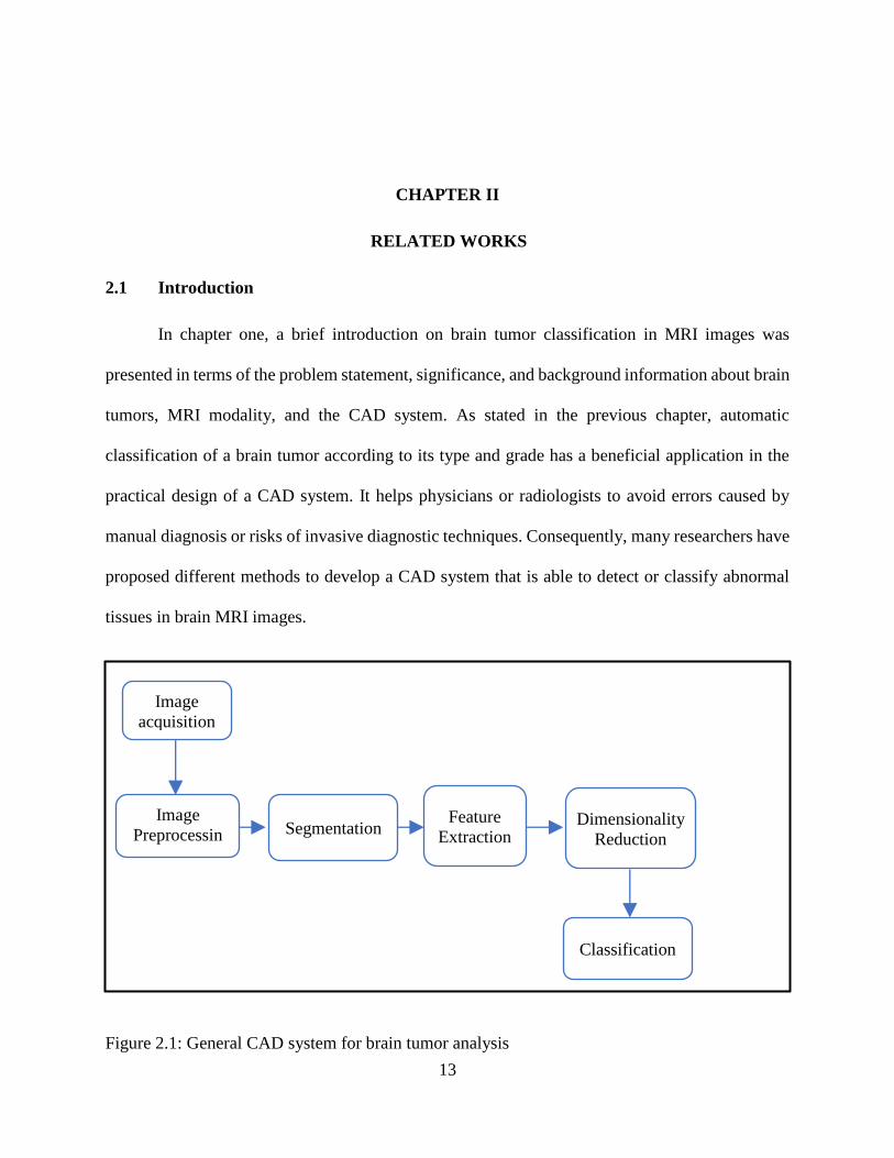
Figure 2.1: General CAD system for brain tumor analysis
Image
acquisition
Image
Preprocessin
g
Segmentation Feature
Extraction Dimensionality
Reduction
Classification
14
This chapter presents a survey on the most recent methods and algorithms that have been
designed for solving the aforementioned problem. A general CAD system is shown in fig. 2.1. It
comprises of the following steps; image acquisition, image preprocessing, segmentation of MRI
image to extract the region of interest (ROI), feature extraction, dimensionality reduction, and
classification [3].
2.2 Classification Approach
There are two kinds of brain tumor classification methods. The first method is classifying
the brain image into normal and abnormal, and the second method is to classify the abnormal brain
image into different types of brain tumors [28]. A few studies have proposed classification
techniques to identify brain images according to normal and abnormal [5], [10], [29]. Other studies
have focused on detecting the abnormality of the tumor and then classify the abnormal tissue into
benign and malignant [4], [8], [30], [31]. Sometimes they may only classify the brain images into
benign and malignant [32]–[34]. Some authors presented multiclass brain tumor classification
methods to identify the type and/or the grade of the tumor [6], [7], [28], [35]–[44].
The type of tumor that has been discussed in these studies are Glioma, Glioblastoma,
Carcinoma, Meningioma, Sarcoma, Astrocytoma, Metastasis, Medulloblastoma, and Pituitary
tumors. In addition, the grade of the tumor is considered in the classification process. In [6] four
grades of Astrocytoma have been considered: grade I, grade II, grade III, and grade IV. Zacharaki
et al [39], [43] discriminate different types and grades of the tumors as: Meningioma tumors are
grade I, Gliomas are grade II and grade III, and Glioblastomas are grade IV.
15
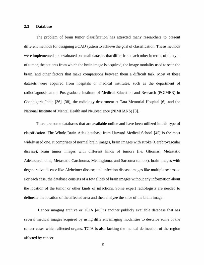
2.3 Database
The problem of brain tumor classification has attracted many researchers to present
different methods for designing a CAD system to achieve the goal of classification. These methods
were implemented and evaluated on small datasets that differ from each other in terms of the type
of tumor, the patients from which the brain image is acquired, the image modality used to scan the
brain, and other factors that make comparisons between them a difficult task. Most of these
datasets were acquired from hospitals or medical institutes, such as the department of
radiodiagnosis at the Postgraduate Institute of Medical Education and Research (PGIMER) in
Chandigarh, India [36]–[38], the radiology department at Tata Memorial Hospital [6], and the
National Institute of Mental Health and Neuroscience (NIMHANS) [8].
There are some databases that are available online and have been utilized in this type of
classification. The Whole Brain Atlas database from Harvard Medical School [45] is the most
widely used one. It comprises of normal brain images, brain images with stroke (Cerebrovascular
disease), brain tumor images with different kinds of tumors (i.e. Gliomas, Metastatic
Adenocarcinoma, Metastatic Carcinoma, Meningioma, and Sarcoma tumors), brain images with
degenerative disease like Alzheimer disease, and infection disease images like multiple sclerosis.
For each case, the database consists of a few slices of brain images without any information about
the location of the tumor or other kinds of infections. Some expert radiologists are needed to
delineate the location of the affected area and then analyze the slice of the brain image.
Cancer imaging archive or TCIA [46] is another publicly available database that has
several medical images acquired by using different imaging modalities to describe some of the
cancer cases which affected organs. TCIA is also lacking the manual delineation of the region
affected by cancer.
16
Menze et al [13] organized a Multimodal Brain Tumor Image Segmentation benchmark
challenge (BRATS). They prepare a dataset of MRI images of low and high-grade glioma patients
and made these datasets publicly available along with its related manual segmentation acquired by
many human experts. The training part of this dataset comprises of 30 patients; 20 with high-grade
tumors and 10 with low-grade tumors. This database has been used for the classification of Glioma
tumor grades as high and low [47]–[49].
Cheng et al [28] implemented their work on a large database which consists of 3,064 slices
collected from 233 patients with three kinds of brain tumors, meningioma, glioma, and pituitary.
These slices were acquired from the Nanfung Hospital in Guangzhou, and the General Hospital of
Tianjing Medical University in China during the period of 2005 to 2010. These slices were
manually segmented by three expert radiologists to generate a tumor mask. The original slices
along with its mask are available online from the Figshare website [50].
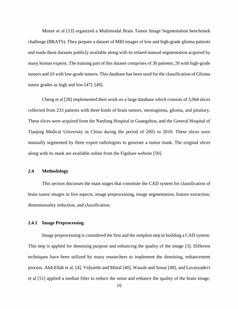
2.4 Methodology
This section discusses the main stages that constitute the CAD system for classification of
brain tumor images in five aspects, image preprocessing, image segmentation, feature extraction,
dimensionality reduction, and classification.
2.4.1 Image Preprocessing
Image preprocessing is considered the first and the simplest step in building a CAD system.
This step is applied for denoising purpose and enhancing the quality of the image [3]. Different
techniques have been utilized by many researchers to implement the denoising, enhancement
process. Abd-Ellah et al. [4], Vidyarthi and Mittal [40], Wasule and Sonar [48], and Lavanyadevi
et al [51] applied a median filter to reduce the noise and enhance the quality of the brain image.
17
Anitha et al. [10] take advantage of the mean filter to reduce the effect of noise by updating the
pixel value using a weighted average of the pixel value. Zulpe et al. [7] applied a Gaussian filter
for denoising and outlier elimination. Singh and Ansari [52] implemented five filters for denoising:
median filter, adaptive filter, Gaussian filter, averaging filter, and un-sharp masking filter. Another
technique for image denoising is 2-D Discrete Wavelet Transform (DWT) which is a powerful
tool for filtering in the wavelet domain and removing the noise using thresholding [42]. Zacharaki
et al. [43] used three preprocessing steps: noise reduction, inhomogeneity correction, and
registration.
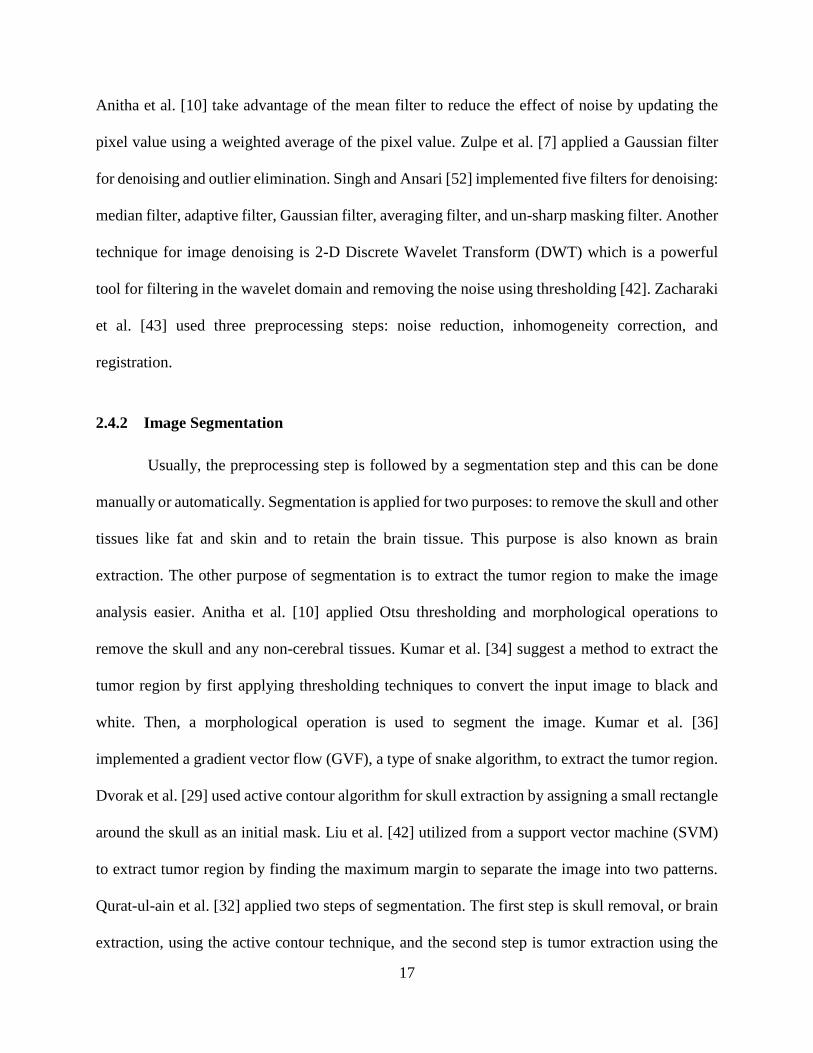
2.4.2 Image Segmentation
Usually, the preprocessing step is followed by a segmentation step and this can be done
manually or automatically. Segmentation is applied for two purposes: to remove the skull and other
tissues like fat and skin and to retain the brain tissue. This purpose is also known as brain
extraction. The other purpose of segmentation is to extract the tumor region to make the image
analysis easier. Anitha et al. [10] applied Otsu thresholding and morphological operations to
remove the skull and any non-cerebral tissues. Kumar et al. [34] suggest a method to extract the
tumor region by first applying thresholding techniques to convert the input image to black and
white. Then, a morphological operation is used to segment the image. Kumar et al. [36]
implemented a gradient vector flow (GVF), a type of snake algorithm, to extract the tumor region.
Dvorak et al. [29] used active contour algorithm for skull extraction by assigning a small rectangle
around the skull as an initial mask. Liu et al. [42] utilized from a support vector machine (SVM)
to extract tumor region by finding the maximum margin to separate the image into two patterns.
Qurat-ul-ain et al. [32] applied two steps of segmentation. The first step is skull removal, or brain
extraction, using the active contour technique, and the second step is tumor extraction using the
18
fuzzy C-mean algorithm. Benson et al. [53] used a fuzzy C-mean algorithm to extract the gray
matter and white matter from MRI brain images.
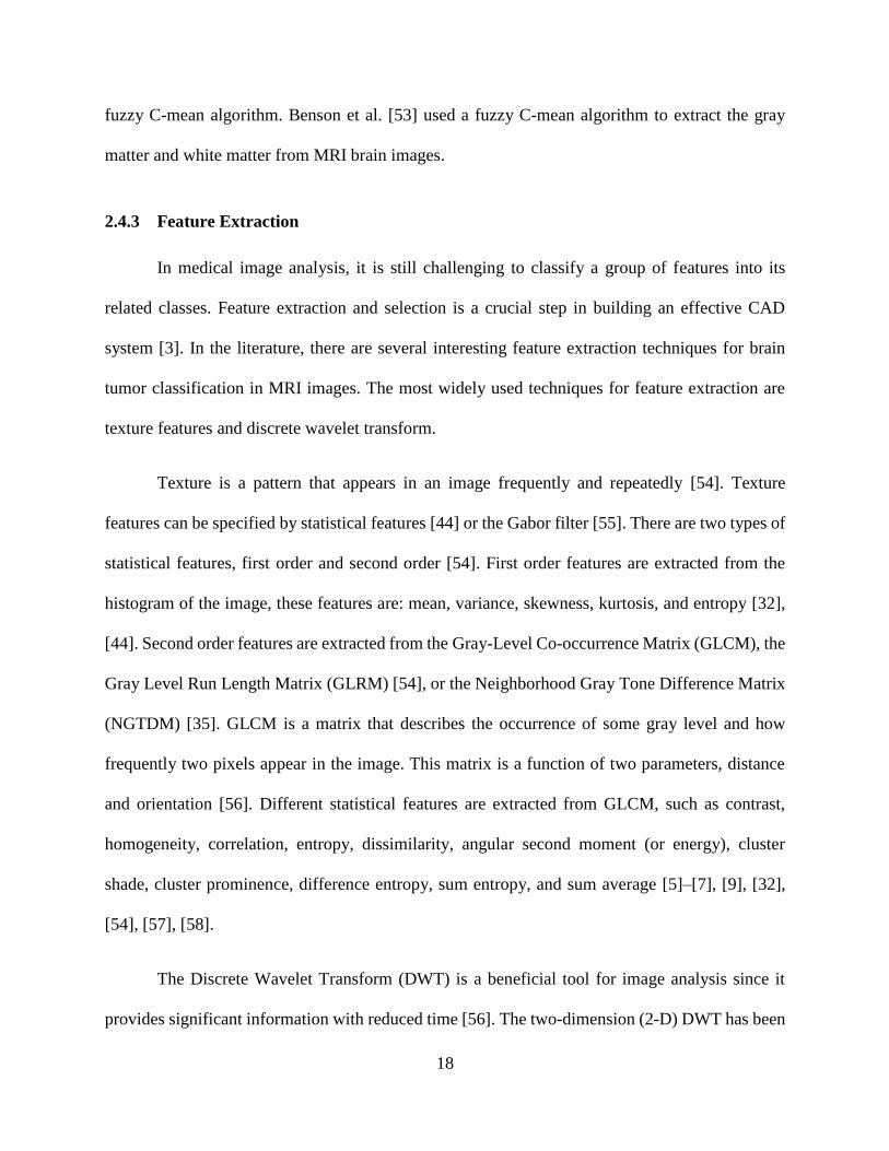
2.4.3 Feature Extraction
In medical image analysis, it is still challenging to classify a group of features into its
related classes. Feature extraction and selection is a crucial step in building an effective CAD
system [3]. In the literature, there are several interesting feature extraction techniques for brain
tumor classification in MRI images. The most widely used techniques for feature extraction are
texture features and discrete wavelet transform.
Texture is a pattern that appears in an image frequently and repeatedly [54]. Texture
features can be specified by statistical features [44] or the Gabor filter [55]. There are two types of
statistical features, first order and second order [54]. First order features are extracted from the
histogram of the image, these features are: mean, variance, skewness, kurtosis, and entropy [32],
[44]. Second order features are extracted from the Gray-Level Co-occurrence Matrix (GLCM), the
Gray Level Run Length Matrix (GLRM) [54], or the Neighborhood Gray Tone Difference Matrix
(NGTDM) [35]. GLCM is a matrix that describes the occurrence of some gray level and how
frequently two pixels appear in the image. This matrix is a function of two parameters, distance
and orientation [56]. Different statistical features are extracted from GLCM, such as contrast,
homogeneity, correlation, entropy, dissimilarity, angular second moment (or energy), cluster
shade, cluster prominence, difference entropy, sum entropy, and sum average [5]–[7], [9], [32],
[54], [57], [58].
The Discrete Wavelet Transform (DWT) is a beneficial tool for image analysis since it
provides significant information with reduced time [56]. The two-dimension (2-D) DWT has been
19
implemented to extract features from brain MRI images for tumor classification [10], [33], [40],
[41]. Applying the 2-D DWT on image results in four images named LL, LH, HL, and HH sub-
bands. These will be described in chapter three.
Statistical features can be extracted from the sub-band images that resulted from the 2-D
DWT. In the literature, some authors extract these features from the LL sub-band image [40], [59],
[60], other works suggested using the LH and HL sub-band images for the statistical features
calculation [8], [61], [62]. The Gabor filter is a linear and local filter that is based on the
convolution between the Gaussian function and the cosine function [55]. Texture features based
on Gabor filter have been employed in the literature to extract the required features for the
classification of a brain tumor. Liu et al. [42] used the Gabor wavelet analysis for extracting
features from the region of interest. The Gabor wavelets are beneficial for orientation selectivity
and spatial locality due to its ability to capture the location structure of the image. Vidyarthi and
Mittal [40] used a hybrid approach to extract features using Gabor filter and DWT. Texture features
extracted from brain images are determined using symmetric and antisymmetric Gabor kernels.
Shingade and Jain [63] proposed a method for brain tumor detection and segmentation using the
Gabor filter and statistical features. Some authors extract the statistical features from the output of
the Gabor filter [36], [38].
Zacharaki et al. [39], [43] used features based on shape and intensity along with Gabor
filter features for classification of brain tumor types and grades. Othman et al. [64] and Sumitra
[30] utilized the principal component analysis to extract useful features from MRI brain images.
Cheng et al. [28] employed three techniques for extracting features from brain MRI images:
GLCM, intensity histogram, and bag of words features. Dvorak et al. [29] used probabilistic maps

20
as feature extraction by calculating the global maximum and block size and then thresholding the
total probabilistic map.
2.4.4 Dimensionality Reduction
The curse of dimensionality is the main challenge that faces the classification process, and
it is caused by unnecessary features generated by feature extraction techniques. These extra
features increase the time and memory storage required for the CAD system implementation [3].
The most commonly used technique in the literature for feature reduction in brain tumor
classification is the Principle Component Analysis (PCA) [4], [33], [34], [36], [38], [41], [49]. The
PCA is an efficient tool that transforms a high dimensional input feature with correlated variables
into a low dimensional uncorrelated feature vector using orthogonal transformation [4], [17].
There are other techniques for feature selection and dimensionality reduction that can be
employed in the classification of a brain tumor. The Genetic Algorithm (GA) is used for features
selection by representing the feature vector as a chromosome and to find the optimal solution to
the fitness function by performing three operations: selection, crossover, and mutation. These
operations will converge after consecutive operations to reach the final optimal solution [37].The
fuzzy entropy measure is another type of feature selection method. It is implemented by the
fuzzification of the feature set and calculating the entropy of the data membership [54]. The
Cumulative Variance Method (CVM) was used by [40] for the selection of features. In addition, it
was examined by using various classification algorithms and then compared with the GA and the
PCA. Zacharaki et al. [39], [43] proposed two methods for feature selection. The first method is
implemented using ranking-based criterion, and the second method is carried out by using the
21
support vector machine feature elimination algorithm. These two methods were compared with the
constrained Linear Discriminant Analysis (LDA).
2.4.5 Classification Techniques
Classification is the most significant step in the CAD system [4] since it gives the final
decision about the required class based on the features extracted from the input image [3]. Many
factors should be considered before choosing the appropriate classifier for brain tumor
classification. These factors are: accuracy, performance, and computational resources [3].
Different classification techniques have been exploited by many authors for identifying tumors in
brain images. The most commonly used classifiers are the neural network and the support vector
machines (SVM).
The neural network is, “a massively parallel distributed processor made up of simple
processing units that has a natural propensity for storing experiential knowledge and making it
available for use” [65]. It has been proved as an efficient tool for classification purposes due to its
ability to adjust themselves to data and approximate any function with arbitrary accuracy [66].
Zulpe et al. [7] presented a classification technique based on two layers of the feedforward
neural network with a sigmoid function. They utilized from Levenberg-Marqurat algorithm to train
their network. Kharat et al [33] developed two classifiers. The first one is implemented using three
layers feedforward neural network with 500, 1 to 50, and 1 neurons in the input, hidden, and output
layers respectively. The second one is based on the back propagation neural network with binary
sigmoid function as the activation function.
Kumar et al. [36] proposed a method for classifying six kinds of brain tumors using
multilayer perceptron neural network. To train this network they utilized the ‘Gradient Descent
22
Back Propagation with the momentum algorithm, where the value of momentum is 0.8 and the
learning rate is 0.02. A 10-fold cross-validation is used to enhance the network by avoiding
overtraining. Sachdeva et al. [38] presented a dual level ensemble classifier based on a neural
network similar to the network in [36]. The ensemble classifier has two levels, upper and lower.
The upper level consists of three layers: the artificial neural network that has 49, 18, and 6 neurons
in the input, hidden, and output layers respectively. The lower level has 15 two-class classifiers
arranged so that each network is mutually independent. Each classifier in the lower level is like
the classifier in the upper level but with 10 neurons in the hidden layer and 2 neurons in the output
layer. The weighted score method, which is stemmed from the principle of ‘winner takes all’, is
utilized to determine the output result. Sudha et al. [54] presented a classification method that
comprises of three artificial neural networks: the first network is a two layers feedforward neural
network, the second network is designed using multilayer perceptron, and the last network has one
hidden layer. The training algorithm for these networks is the back-propagation algorithm
implemented using the ‘scaled conjugate gradient’ optimization algorithm and the sigmoid
activation function. Sumitra [30] proposed an algorithm that constitutes the three layers neural
network with 15, 1 to 15, and 1 neurons in the input, hidden, and output layers respectively. The
learning algorithm for tuning the weights and biases of the network is the back-propagation
algorithm. The activation function used in this method is the binary sigmoid function which limits
the output to be between 0 and 1.
The probabilistic neural network (PNN) is a type of neural network that is based on
Bayesian classifier techniques and it is designed to overcome the time limitation of the multilayer
perceptron architecture [67]. John [8] presented a probabilistic neural network with three layers,
the input layer, radial basis layer, and competitive layer. Othman et al. [64] used a probabilistic
23
neural network that is implemented with different spread values which was considered as the
smoothing factor of the radial basis function. The Learning Vector Quantization (LVQ) is a type
of neural network introduced by Kohonen [68] and it consists of three layers: input layer,
competitive layer, and output layer. Sonavane et al. [57] presented a classification technique using
the LVQ network for abnormality detection in brain images.
The Support vector machine (SVM) is a new type of classifier based on a statistical learning
technique that minimizes the error by maximizing the margin between the separating hyperplane
and the data [69]. Javed et al. [35] implemented a classification method using the SVM with a ‘one
versus all’ technique. In this technique, several binary SVM classifiers (equal to the number of
classes) are designed so that one class is considered positive and the others are considered negative.
Zhang et al. [41] proposed a classification technique based on the kernel SVM, which was
implemented by using three kernels: homogenous polynomial, inhomogeneous polynomial, and
Gaussian radial basis function. They integrated a cross-validation method into the classifier model
to avoid overfitting. Three types of cross-validation are: random subsampling, k-fold cross-
validation, and leave-one-out validation. They applied k-fold cross-validation and calculated the
best value of k to be 5 using trial and error method. In the k-fold cross-validation, the whole dataset
is divided into (k) partitions. Then, (k-1) of these partitions are used for training and the remaining
partition is used for validation, and this process will be repeated k times. Kumar et al. [34] designed
an SVM classifier with three kernels. These three kernels are a linear kernel, a Gaussian or radial
basis function, and a polynomial kernel. Abd-Ellah et al. [4] developed a CAD system that has two
classification stages. In the first stage, they used kernel SVM with Gaussian radial basis function
to classify MRI images into normal and abnormal. In the second stage, they implemented the
kernel SVM using the linear kernel to classify MRI images into benign and malignant. Zacharaki
24
et al. [43] used a nonlinear binary SVM classifier with the Gaussian kernel to identify different
types and grades of brain tumors. They used the weighted SVM to apply a penalty to the class with
fewer samples. The ‘one-versus-all’ method is applied to benefit from this binary SVM and is used
for multi-class classification. In addition, they implement ‘leave-one-out cross-validation’
algorithm to test the ability of the classifier model. Mohana et al. [44] proposed an algorithm based
on two types of SVM classifiers. The first one is called ‘n-SVM’ and it is implemented to classify
Astrocytoma grades using the radial basis function kernel. The second one is called ‘c-SVM’ and
it is used for classification of tumor types using the polynomial kernel. Halder and Dobe [70] used
the SVM classifier for detection of abnormal brain tissue using statistical features.
Few studies employed different types of classifier models to build their algorithms. GA
and SVM were used by [37] as classification techniques to generate a CAD system that is able to
classify five types of tumors in MRI images. In this algorithm, the SVM was implemented using
the Gaussian kernel function. Zacharaki et al. [39] employed three different classifiers, non-linear
SVM, k-nearest neighbor (KNN), and Linear discriminant analysis (LDA). SVM is implemented
using radial basis function kernel while LDA is implemented with fisher’s discriminate rule. The
performance of these classifiers was validated using leave-one-out cross-validation method.
Selvaraj et al. [5] used four classification techniques: the multilayer perceptron neural network,
the feedforward neural network based on radial basis function, the KNN, and the least squares
SVM with two kernels (radial basis function and linear kernel). The performance of the least square
SVM was the best as compared to other classifiers. Anitha et al. [10] proposed a two-stage
classification approach to identify abnormal tissues in MRI images. In the first stage, an
unsupervised learning method is used to train the wavelet features and it is based on the Self-
Organizing Map (SOM). The SOM is a kind of neural network that is trained using the competitive

25
learning method. In the second stage, a supervised learning algorithm is implemented using the
KNN classifier to train the features. Vidyarthi and Mittal [40] proposed an approach for brain
tumor classification that employed three classification models, which are the back propagation
neural network, the multilevel SVM, and the KNN. The best performance in term of accuracy was
achieved by using the neural network classifier. Qurat-Ul-Ain et al. [32] proposed a classification
method that utilized from the ensemble base classifier for MRI brain tumor diagnosis. A few binary
SVM classifiers were created to classify the brain images into benign and malignant and their
results were combined using algebraic rules. Ahmmed et al. [71] used the SVM classifier for tumor
detection then, the tumor images were classified into benign and malignant using the Artificial
Neural Network (ANN). Farhi and Yusuf [49] proposed a classification technique using five
different classifiers: ANN, Decision tree, KNN, Nave Bayes, and SVM.
Other types of classifiers were employed by some authors, such as the ensemble learning
method based on the AdaBoost classifier [72], the neuro-fuzzy classifier [6], and dictionary
learning and sparse coding [9]. Ghanavati et al. [72] proposed an algorithm for automatic detection
of brain tumors using the AdaBoost classifier. The classifier is used to select the most
discriminative features and to segment the tumor area. They used a ground truth Multi-modal MRI
images to train and validate their method. Joshi et al. [6] used neuro-fuzzy logic to implement a
classification system for brain cancer. They used the artificial neural network and the graphical
user interface for the detection and classification of the tumor. The system was implemented on
MRI images acquired from the Tata Memorial Hospital department of Radiology. In addition, it
shows that this system can be implemented on other types of cancers using other imaging
modalities like the Positron emission tomography (PET) and the Computed tomography (CT). Al-
Shaikhli et al. [9] proposed an algorithm for multiclass brain tumor classification based on sparse

26
coding and dictionary learning. They used two types of classifiers, sparse coding and linear SVM.
They proved that sparse representation outperforms the linear SVM classifier in classification
accuracy.

27
CHAPTER III
3.THE PROPOSED FRAMEWORK: BRAIN TUMOR CLASSIFICATION USING A
HYBRID DOMAIN BASED STATISTICAL FEATURES
3.1 Introduction
As stated in chapter two, classification of brain tumor using MRI image is a crucial step in
the diagnosis of a tumor in the brain. Therefore, many researchers have proposed several
algorithms to identify the type and/or the grade of brain tumor.
Three types of brain tumors are considered in this work; Meningioma, Glioma (both high-
grade and low-grade), and Pituitary.
Table 3.1: Tumor types/grades descriptions
Tumor Description
Meningioma
• Homogeneous
• High-intensity region (brighter than the surrounding regions)
• Appears as extra-axial masses
Glioma
• Heterogeneous
• Low-intensity region (darker than the surrounding regions)
• The tumor border is brighter than the inside
• Low-grade Glioma shows a dark area
• High-grade Glioma shows white area on the border and dark area in the
middle, called necrosis
Pituitary
• Heterogeneous
• The intensity of tumor ranging from high to low
• Appears as a bulk of the gland on the side of the microadenoma

28
while figure 3.1 shows samples of MRI images with the three tumor types and the two grades of
Glioma.
Figure 3.1: MRI sample images showing the three types of tumors and the two grades of Glioma
Tumor
As shown in table 3.1, the main concerns in describing these types/grades of brain tumors
are the intensity and texture of the tumor region. Statistical features represented by the first and
second order statistics can be used to serve as other features for identification of these types/grades
of brain tumors in combinations of machine learning algorithms and large datasets. First order
statistics are extracted from the raw image histogram. The second order statistics are extracted
from the Gray Level Co-occurrence Matrix (GLCM) that describes how frequently the occurrence
two pixels occur, and shows it is a powerful tool for texture description.
(a) Meningioma (b) Glioma (c) Pituitary
(a) High-grade Glioma (b) Low-grade Glioma
29
These statistical features have been used widely in the literature for the task of brain tumor
classification. It can be extracted from the original image in the spatial domain [5], [7], [9], [32],
[57], [58]. On the other hand, these features can be extracted from the transform domain such as
the wavelet transform domain [40], [59], [60], [61], [62] or the Gabor filter domain [36], [38].
Since using the statistical features from the spatial domain/image space is insufficient for
tumor discrimination, another set of features must be found. Indeed, a better feature representation
and a model that has a higher level of accountability of all tumors’ characteristics are a must to
enhance classification results.
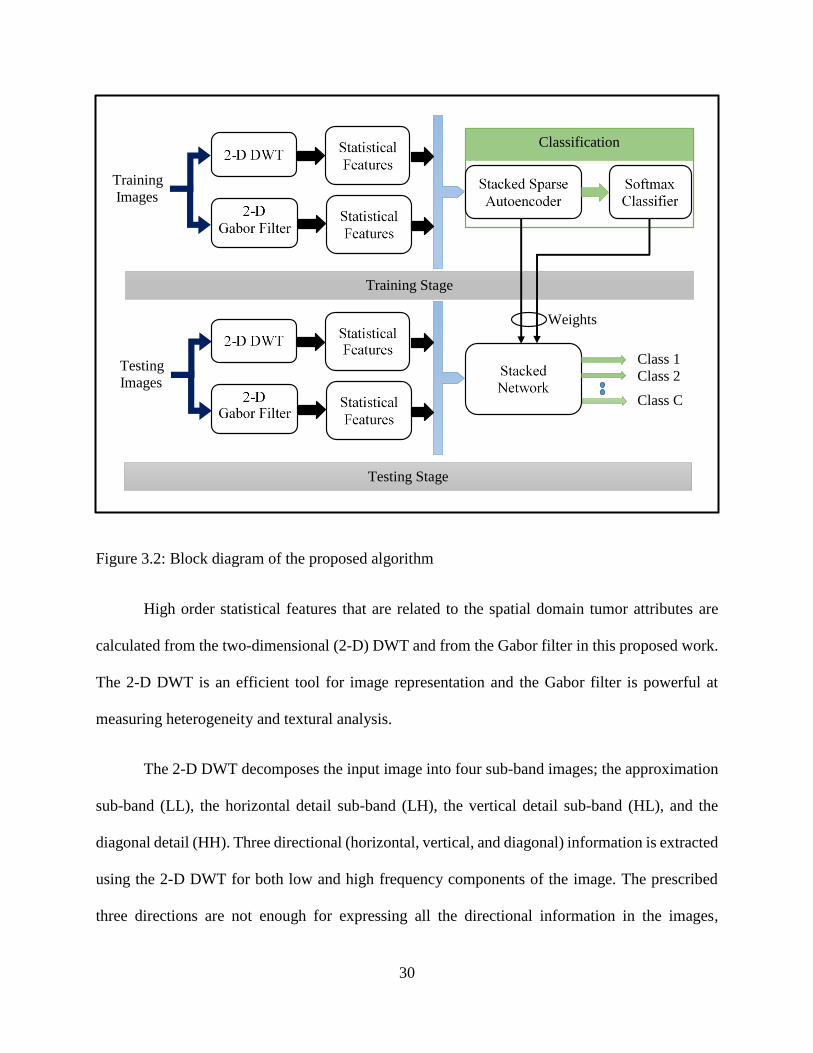
3.2 The Framework of the Proposed System
The proposed algorithm consists of two phases, the training phase and the testing phase,
shown in fig. 3.2. In each phase there are two main steps: feature extraction, and classification.
Feature extraction step is implemented using a combination of the 2-D DWT and the Gabor filter
followed by a statistical calculation. In the classification step, the stacked sparse autoencoder is
trained and stacked with the Softmax classifier during the training step, then it is used to classify
the generated features to its classes in the testing phase.
The input image in each phase (training and testing) is the tumor region that can be
extracted manually by a radiologist or automatically using an automatic segmentation algorithm.
The extracted tumor region is called Region of Interest (ROI) since the focus of MRI image
processing is on this region only. In the following sections, the 2-D DWT, the Gabor filter, and
the statistical features are presented as feature extraction techniques. This is followed by
classification using the Stacked Sparse Autoencoder and the Softmax classifier.
30
Figure 3.2: Block diagram of the proposed algorithm
High order statistical features that are related to the spatial domain tumor attributes are
calculated from the two-dimensional (2-D) DWT and from the Gabor filter in this proposed work.
The 2-D DWT is an efficient tool for image representation and the Gabor filter is powerful at
measuring heterogeneity and textural analysis.
The 2-D DWT decomposes the input image into four sub-band images; the approximation
sub-band (LL), the horizontal detail sub-band (LH), the vertical detail sub-band (HL), and the
diagonal detail (HH). Three directional (horizontal, vertical, and diagonal) information is extracted
using the 2-D DWT for both low and high frequency components of the image. The prescribed
three directions are not enough for expressing all the directional information in the images,
Classification
Training Stage
Testing Stage
Weights
Class 1
Class 2
Class C
Training
Images
Testing
Images
31
especially medical images. Thus, other types of transformation such as the Gabor filter are needed
for better directional representation [73].
The Gabor filter analyzes the edges of the input image producing several images with
different wavelengths and orientations. In addition, it captures visual properties represented by
spatial localization, orientation selectivity, and spatial frequency [74]. To utilize all the directional
information of the input MRI image, the 2-D DWT and the Gabor filter are combined in this
algorithm as directional transformation methods and the statistical features are calculated from the
resulting images for classification purposes. Combining the DWT and the Gabor filter can improve
the classification accuracy as compared to using each method separately.
3.3 Feature Extraction
Feature extraction is the most significant stage in the design of a CAD system for
classification of brain tumors. The choice of feature extraction and selection technique play a vital
role in the performance of the classifier [56]. In this section, three most widely used feature
extraction techniques are applied. This included the 2-D DWT, the 2-D Gabor filter, and the
statistical features represented by the first and second order statistics.
3.3.1 Discrete Wavelet Transform
Representing an image using the Fourier transform gives the only frequency content
information of the image without any spatial localization. It is essential to use a short space window
for the analysis of space localization [56]. Wavelet Transform (WT) is a powerful tool that
transforms the signal from time domain into wavelet domain to analyze the time and frequency
contents at the same time [42].

32
For the high frequencies signal, the Wavelet Transform gives high time resolution and low
frequency resolution, and for low frequencies signal it gives high frequency resolution and low
time resolution. A basis function called “mother wavelet” is scaled and translated to achieve the
time and frequency resolution. Wavelet basis function is generated from the mother wavelet as
follows [75][76]:
𝜓𝑎,𝑏(𝑥) =1
√𝑎𝜓(
𝑥−𝑏
𝑎) , 𝑎 , 𝑏 ∈ 𝑍 ( 𝑎 > 0) (3. 1)
where ψ(x), is the mother wavelet, and (a, b) represent the dilation and translation parameters
respectively.
The Continuous Wavelet Transform (CWT) is the transformation of continuous function
f(x) into another function of two variables Wψ(a, b) and it is defined as follows [77]:
𝑊𝜓(𝑎, 𝑏) = ∫ 𝑓(𝑥)∞
−∞𝜓𝑎,𝑏(𝑥) 𝑑𝑥 (3. 2)
The Discrete Wavelet Transform (DWT) is derived from CWT where dilation and
translation parameters are discretized to provide a time-efficient calculation [56]. The
discretization is performed by setting the dilation and translation parameters as below [78]:
𝑎 = 𝑎𝑜𝑗, 𝑎𝑛𝑑 𝑏 = 𝑘 𝑎 𝑜
𝑗𝑏𝑜 , 𝑓𝑜𝑟 (𝑗, 𝑘) ∈ 𝑍 (3. 3)
where ao > 1 is a dilated step and bo ≠ 0 is a translation step.
The wavelet dilation and translation parameters are discretized dyadically in many of
practical application [79]. Where ao = 2, and bo = 1, a wavelet transform is described as the
standard DWT [80]. The family of standard DWT is given by [77]:
𝜓𝑗,𝑘(𝑥) = 2𝑗
2𝜓(2𝑗𝑥 − 𝑘) (3. 4)
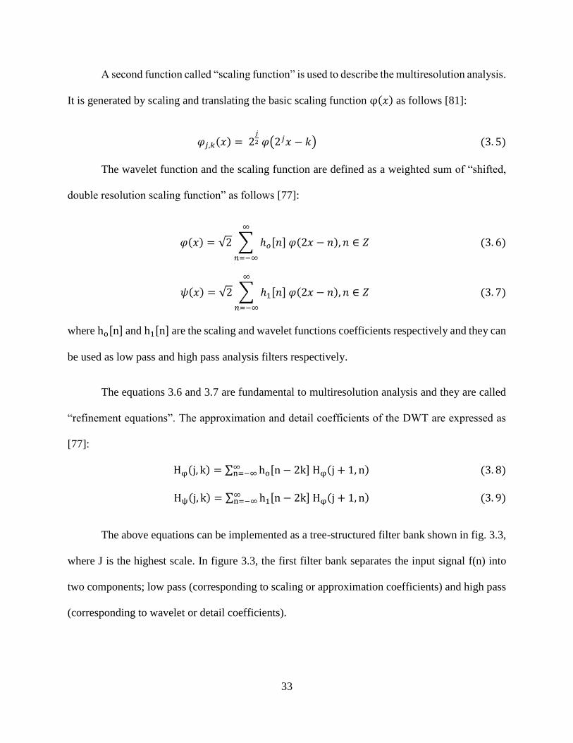
33
A second function called “scaling function” is used to describe the multiresolution analysis.
It is generated by scaling and translating the basic scaling function φ(𝑥) as follows [81]:
𝜑𝑗,𝑘(𝑥) = 2𝑗
2 𝜑(2𝑗𝑥 − 𝑘) (3. 5)
The wavelet function and the scaling function are defined as a weighted sum of “shifted,
double resolution scaling function” as follows [77]:
𝜑(𝑥) = √2 ∑ ℎ𝑜[𝑛] 𝜑(2𝑥 − 𝑛), 𝑛 ∈ 𝑍
∞
𝑛=−∞
(3. 6)
𝜓(𝑥) = √2 ∑ ℎ1[𝑛] 𝜑(2𝑥 − 𝑛), 𝑛 ∈ 𝑍
∞
𝑛=−∞
(3. 7)
where ho[n] and h1[n] are the scaling and wavelet functions coefficients respectively and they can
be used as low pass and high pass analysis filters respectively.
The equations 3.6 and 3.7 are fundamental to multiresolution analysis and they are called
“refinement equations”. The approximation and detail coefficients of the DWT are expressed as
[77]:
Hφ(j, k) = ∑ ho[n − 2k] Hφ(j + 1, n)∞n=−∞ (3. 8)
Hψ(j, k) = ∑ h1[n − 2k] Hφ(j + 1, n)∞n=−∞ (3. 9)
The above equations can be implemented as a tree-structured filter bank shown in fig. 3.3,
where J is the highest scale. In figure 3.3, the first filter bank separates the input signal f(n) into
two components; low pass (corresponding to scaling or approximation coefficients) and high pass
(corresponding to wavelet or detail coefficients).
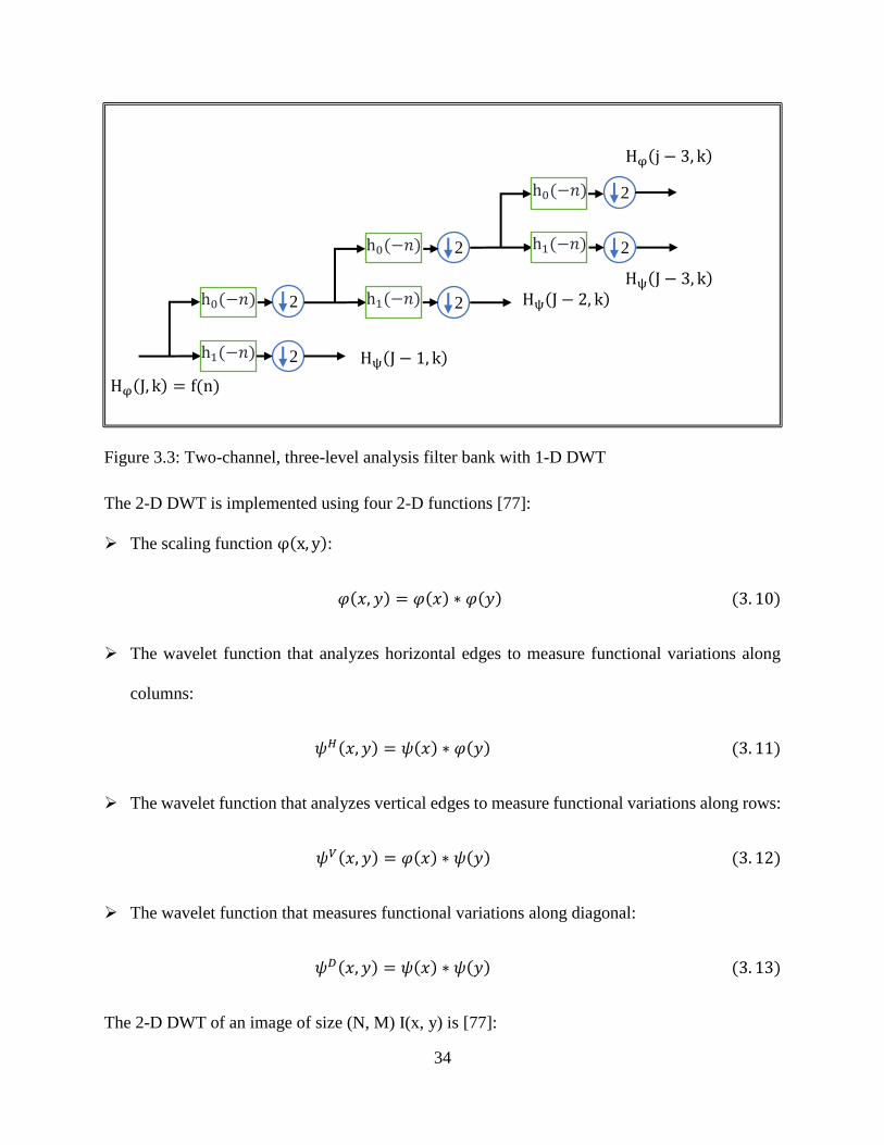
34
Figure 3.3: Two-channel, three-level analysis filter bank with 1-D DWT
The 2-D DWT is implemented using four 2-D functions [77]:
➢ The scaling function φ(x, y):
𝜑(𝑥, 𝑦) = 𝜑(𝑥) ∗ 𝜑(𝑦) (3. 10)
➢ The wavelet function that analyzes horizontal edges to measure functional variations along
columns:
𝜓𝐻(𝑥, 𝑦) = 𝜓(𝑥) ∗ 𝜑(𝑦) (3. 11)
➢ The wavelet function that analyzes vertical edges to measure functional variations along rows:
𝜓𝑉(𝑥, 𝑦) = 𝜑(𝑥) ∗ 𝜓(𝑦) (3. 12)
➢ The wavelet function that measures functional variations along diagonal:
𝜓𝐷(𝑥, 𝑦) = 𝜓(𝑥) ∗ 𝜓(𝑦) (3. 13)
The 2-D DWT of an image of size (N, M) I(x, y) is [77]:
h0(−𝑛)
h1(−𝑛)
2
2
h0(−𝑛)
h1(−𝑛)
2
2
h0(−𝑛)
h1(−𝑛)
2
2
Hφ(J, k) = f(n)
Hψ(J − 1, k)
Hψ(J − 2, k)
Hφ(j − 3, k)
Hψ(J − 3, k)

35
𝐻𝜑(𝑗0,𝑚, 𝑛) =1
√𝑀𝑁∑ ∑ 𝐼(𝑥, 𝑦) ∗ 𝜑𝑗0,𝑚,𝑛(𝑥, 𝑦)
𝑁−1
𝑦=0
𝑀−1
𝑥=0
(3. 14)
𝐻𝜑𝑖 (𝑗,𝑚, 𝑛) =
1
√𝑀𝑁∑ ∑ 𝐼(𝑥, 𝑦) ∗ 𝜓𝑗,𝑚,𝑛
𝑖 (𝑥, 𝑦)
𝑁−1
𝑦=0
𝑀−1
𝑥=0
, 𝑖 = {𝐻, 𝑉, 𝐷} (3. 15)
Where,
𝜑𝑗0,𝑚,𝑛(𝑥, 𝑦) = 2𝑗2 𝜑(2𝑗𝑥 − 𝑚, 2𝑗𝑦 − 𝑛) (3. 16)
𝜓𝑗,𝑚,𝑛𝑖 (𝑥, 𝑦) = 2
𝑗2 𝜓𝑖(2𝑗𝑥 − 𝑚, 2𝑗𝑦 − 𝑛), 𝑖 = {𝐻, 𝑉, 𝐷} (3. 17)
j0: is an arbitrary starting scale
The implementation of an analysis filter bank for a single level 2-D DWT is shown in fig.
3.4 [23]. By applying 2-D DWT, the image is decomposed into four sub-bands labeled LL, LH,
HL, and HH. The LH, HL and HH sub-bands represent the wavelet or detail coefficients of the
image HφH(j,m, n), Hφ
V(j,m, n), and HφD(j,m, n) respectively.
Figure 3.4: One level filter bank for computation of 2-D DWT
h0(−𝑛)
h1(−𝑛)
2
2
h0(−𝑛)
h1(−𝑛)
2
2
h0(−𝑛)
h1(−𝑛)
2
2
LL
LH
HL
HH
Input
Image

36
The sub-band LL corresponds to scaling or approximation coefficients of the image
Hφ(j0,m, n) [77], [81]. Fig. 3.5 shows the sub-band decomposition for two levels of the 2-D DWT
implemented on an image.
Figure 3.5: Image Decomposition using 2-levels of 2-D DWT
3.3.2 Gabor Filter
In 1946, Dennis Gabor [82] introduced Gabor filter for signal representation in both time
and frequency domain. A Gabor filter is a linear filter that is obtained by modulating a sinusoidal
wave with a Gaussian function [83]. In other words, it is generated by convolving a Gaussian
function by a complex sinusoidal wave with different frequencies and orientations [84]. The
frequency and orientation of the Gabor filter are similar to the human visual system and it can be
used for texture description [85]. The Gabor function is a useful tool in computer vision and image
processing, especially for texture analysis, due to its optimal localization properties in both spatial
and frequency domains [86]. The Gabor filter is able to analyze 1-D or 2-D signals in both spatial
and frequency domain [84]. The 2-D Gabor filter is defined as [55]:
Input
Image
2-levels of
2-D DWT
LL2 LH2
HL2 HH2
LH1
HH1 HL1

37
𝐺(𝑥, 𝑦, 𝜆, 𝜃, 𝜙, 𝜎, 𝛾) = 𝑒−
𝑥′2+𝛾2𝑦′
2𝜎2 ∗ 𝑒𝑖 (2𝜋
𝑥′
𝜆+𝜓)
(3. 18)
Where:
➢ 𝑥′ = 𝑥 𝑐𝑜𝑠(𝜃) + 𝑦 sin(𝜃)
➢ 𝑦′ = − 𝑥 𝑐𝑜𝑠(𝜃) + 𝑦 sin(𝜃)
➢ λ: is the wavelength of the sinusoidal form
➢ 𝜃: is the orientation of the Gabor function
➢ 𝜙: is the phase offset
➢ 𝛾: is the spatial aspect ratio
𝜎 : is the standard deviation of the Gaussian envelope
Fig. 3.6 shows the shape of Gabor filter with two wavelengths 2 and 4, and two orientations 0 and
90.
In order to get a Gabor feature from an image 𝐼(𝑥, 𝑦), a 2-D convolution is performed
between the image and the 2-D Gabor function as follows [55]:
𝐼𝐺(𝑥, 𝑦) = ∬𝐼(𝑟, 𝑠) ∗ 𝐺(𝑥 − 𝑟, 𝑦 − 𝑠) 𝑑𝑟 𝑑𝑠
∞
−∞
(3. 19)
Where (𝐼𝐺) is the filtered image.
Another approach used to analyze the Gabor filter is by taking the Fourier transform of the
image and multiplying it by the Gaussian function centered at various frequencies and taking the
Inverse Fourier Transform of the results. The choice of the central frequency of each Gaussian is
important to ensure all the frequencies of the image are covered [84].

38
Figure 3.6: Gabor filter shape with different wavelengths and orientations, (a) 𝜆 = 2, 𝜃 = 0°, (b)
𝜆 = 2, 𝜃 = 90°, (c) 𝜆 = 4, 𝜃 = 0°, and (d) 𝜆 = 4, 𝜃 = 90°
Another method to describe the Gabor filter features is using the Gabor energy quantity
which can be calculated by combining a symmetric and an antisymmetric kernel filter in each
image as shown in fig. 3.7. The Gabor energy feature is like the selectivity property of neuron in
the visual cortex. The Gabor energy can be expressed as follows:
𝐺𝑒(𝑥, 𝑦) = √𝐺2(𝑥, 𝑦, 𝜆, 𝜃, 𝜓 = 0) + 𝐺2(𝑥, 𝑦, 𝜆, 𝜃, 𝜓 = 90) (3. 20)
Where:
➢ 𝐺2(x, y, 𝜆, 𝜃, 𝜓 = 0): is the symmetric Gabor filter
(a)
(c)
(d)
(b)

39
➢ 𝐺2(x, y, 𝜆, 𝜃, 𝜓 = 90): is the antisymmetric Gabor filter
Figure 3.7: Gabor filter shape with the symmetric and antisymmetric kernel, (a) 𝜆 = 4, 𝜃 =90°, 𝜓 = 0°, (b) 𝜆 = 4, 𝜃 = 90°, 𝜓 = 90°
The Gabor energy and local power spectrum are related together using the Fourier
transform of the image and a Gaussian windowing function [55].
3.3.3 Statistical Features
The texture of an image can be described easily using a statistical approach [77]. Two
types of statistical approaches are considered in this section:
3.3.3.1 First Order Statistics
First order statistics are calculated from the histogram of the image since the histogram
give the statistical information about an image [32]. Fig. 3.8 shows an example of calculating the
histogram of an image. Histogram of an image is a discrete function of the image intensity levels
in the range [0, L-1], it is defined as follows [77]:
𝑃(𝑖) =𝑛𝑖
𝑁𝑀, 𝑖 = 0, 1, 2, … , 𝐿 − 1 (3. 21)
(a)
(b)
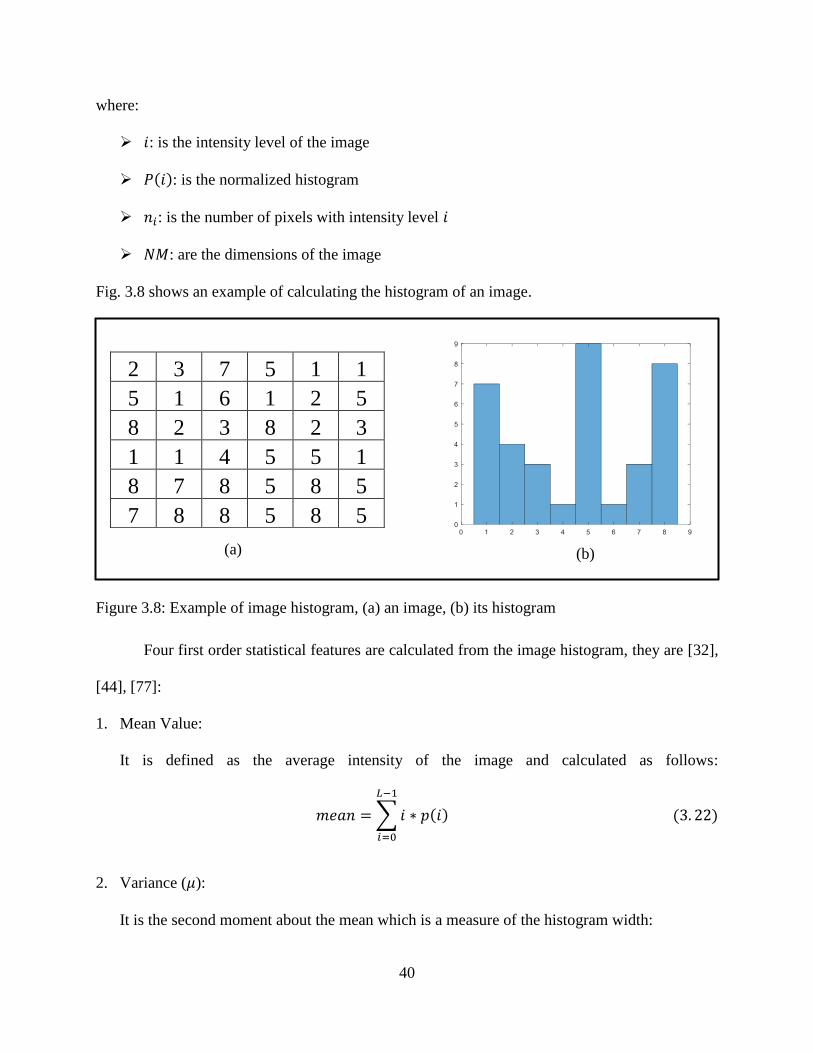
40
where:
➢ 𝑖: is the intensity level of the image
➢ 𝑃(𝑖): is the normalized histogram
➢ 𝑛𝑖: is the number of pixels with intensity level 𝑖
➢ 𝑁𝑀: are the dimensions of the image
Fig. 3.8 shows an example of calculating the histogram of an image.
Figure 3.8: Example of image histogram, (a) an image, (b) its histogram
Four first order statistical features are calculated from the image histogram, they are [32],
[44], [77]:
1. Mean Value:
It is defined as the average intensity of the image and calculated as follows:
𝑚𝑒𝑎𝑛 = ∑𝑖 ∗ 𝑝(𝑖)
𝐿−1
𝑖=0
(3. 22)
2. Variance (𝜇):
It is the second moment about the mean which is a measure of the histogram width:
2 3 7 5 1 1
5 1 6 1 2 5
8 2 3 8 2 3
1 1 4 5 5 1
8 7 8 5 8 5
7 8 8 5 8 5
(a) (b)

41
𝜇 = ∑(𝑖 − 𝑚)2 ∗ 𝑝(𝑖)
𝐿−1
𝑖=0
(3. 23)
3. Skewness (SK):
The skewness is the third moment about the mean. It is considered as a measurement of the
asymmetry of the histogram around the sample mean:
𝑆𝐾 = ∑(𝑖 − 𝑚)3 ∗ 𝑝(𝑖)
𝐿−1
𝑖=0
(3. 24)
4. Kurtosis (𝐾)
The kurtosis is the fourth moment about the mean and it represents the flatness of the
histogram. It is shown with the below equation:
𝐾𝑢 = ∑(𝑖 − 𝑚)4 ∗ 𝑝(𝑖)
𝐿−1
𝑖=0
(3. 25)
3.3.3.2 Second Order Statistics
Texture features measured using first order statistics have no information about the
adjacent pixels with respect to each other which is significant for texture description. Therefore, a
matrix called “Gray Level Co-occurrence Matrix (GLCM)” is defined to describe the relative
information between two adjacent pixels [77]. The GLCM is a 2-D histogram that describes the
frequency of occurrence of two pixels separated by a certain distance d. To describe the GLCM,
suppose that 𝐼(𝑥, 𝑦) be an image with size N × M, and with gray levels (0, L-1), and (a1, b1) and
(a2, b2) be two pixels with intensity levels 𝑖 and 𝑗, respectively. When taking Δa = 𝑎2 − 𝑎1 in the
𝑥 direction and 𝛥b = 𝑏2 − 𝑏1 in the y direction, the connecting straight line has a direction θ
which is equal to 𝑡𝑎𝑛−1 𝛥a
𝛥b . The element of co-occurrence matrix is calculated as [17]:
42
𝐺𝐿𝐶𝑀 (𝑖, 𝑗) = (𝑁𝑢𝑚 ((𝑎1, 𝑏1), (𝑎2, 𝑏2)) ∈ (𝑁 × 𝑀) × (𝑁 × 𝑀)|𝐴) (3. 26)
where:
➢ A: is a given condition, such as Δa = d ∗ sinθ, Δb = d ∗ cosθ, I(a1, b1) = i, and
I(a2, b2) = j
➢ Num: is the number of elements in the co-occurrence matrix
The size of the GLCM matrix is determined by the number of intensity levels in the image.
For example, if the possible intensity levels of the image are 256, then the size of GLCM matrix
will be (256 x 256). To reduce the computation load and make the size of GLCM manageable, an
approach is applied on GLCM to quantize the intensity levels into a few bands. For the case of 256
intensity levels, this quantization is carried out by making the first 32 intensity levels equal to 1,
the next 32 equals to 2 and so on. The total number of the pairs of pixels (NP) is equal to the sum
of the elements of GLCM, then the probability that a pair of pixels will have values
(a1, b1), (a2, b2) is [77]:
P (i, j) =GLCM (i, j)
NP, P (i, j) ∈ [0, 1] (3. 27)
Figure 3.9: Example of a GLCM matrix generation, (a) an image, (b) its GLCM matrix
2 3 7 5 1 1
5 1 6 1 2 5
8 2 3 8 2 3
1 1 4 5 5 1
8 7 8 5 8 5
7 8 8 5 8 5
1 2 3 4 5 6 7 8
1 2 1 0 1 0 1 0 0
2 0 0 3 0 1 0 0 0
3 0 0 0 0 0 0 1 1
4 0 0 0 0 1 0 0 0
5 3 0 0 0 1 0 0 2
6 1 0 0 0 0 0 0 0
7 0 0 0 0 1 0 0 2
8 0 2 0 0 4 0 1 1
(b) (a)

43
Fig. 3.9 shows an example of a GLCM generation, where the matrix on the left is the input
image 𝐼(𝑥, 𝑦) and the matrix on the right is the GLCM. In the above example, the pair of pixels
(2, 3) appears three times in the image, this will result in a value of three in the second row and
third column of the GLCM.
After generating a GLCM matrix of size (B x B) from an image, some useful second order
statistics can be extracted from this matrix. Six of these statistics are described below [44], [77]:
1. Contrast:
It is the measure of the local variations in the GLCM and defined as follows:
𝐶𝑜𝑛𝑡𝑟𝑎𝑠𝑡 = ∑∑(𝑖 − 𝑗)2 𝑝(𝑖, 𝑗)
𝐵
𝑗=1
𝐵
𝑖=1
(3. 28)
2. Correlation:
It is the measure of the correlation of a pixel with its neighbor in an image. It is calculated as
follows:
𝐶𝑜𝑟𝑟𝑒𝑙𝑎𝑡𝑖𝑜𝑛 = ∑∑(𝑖 − 𝑚1) (𝑗 − 𝑚2) 𝑝(𝑖, 𝑗)
𝜎1𝜎2
𝐵
𝑗=1
𝐵
𝑖=1
(3. 29)
3. Energy:
Energy or angular second moment is a measure of smoothness of the image and uniformity in
the range [0, 1]. It is calculated as:
𝐸𝑛𝑒𝑟𝑔𝑦 = ∑∑(𝑝(𝑖, 𝑗))2
𝐵
𝑗=1
B
𝑖=1
(3. 30)
4. Homogeneity:
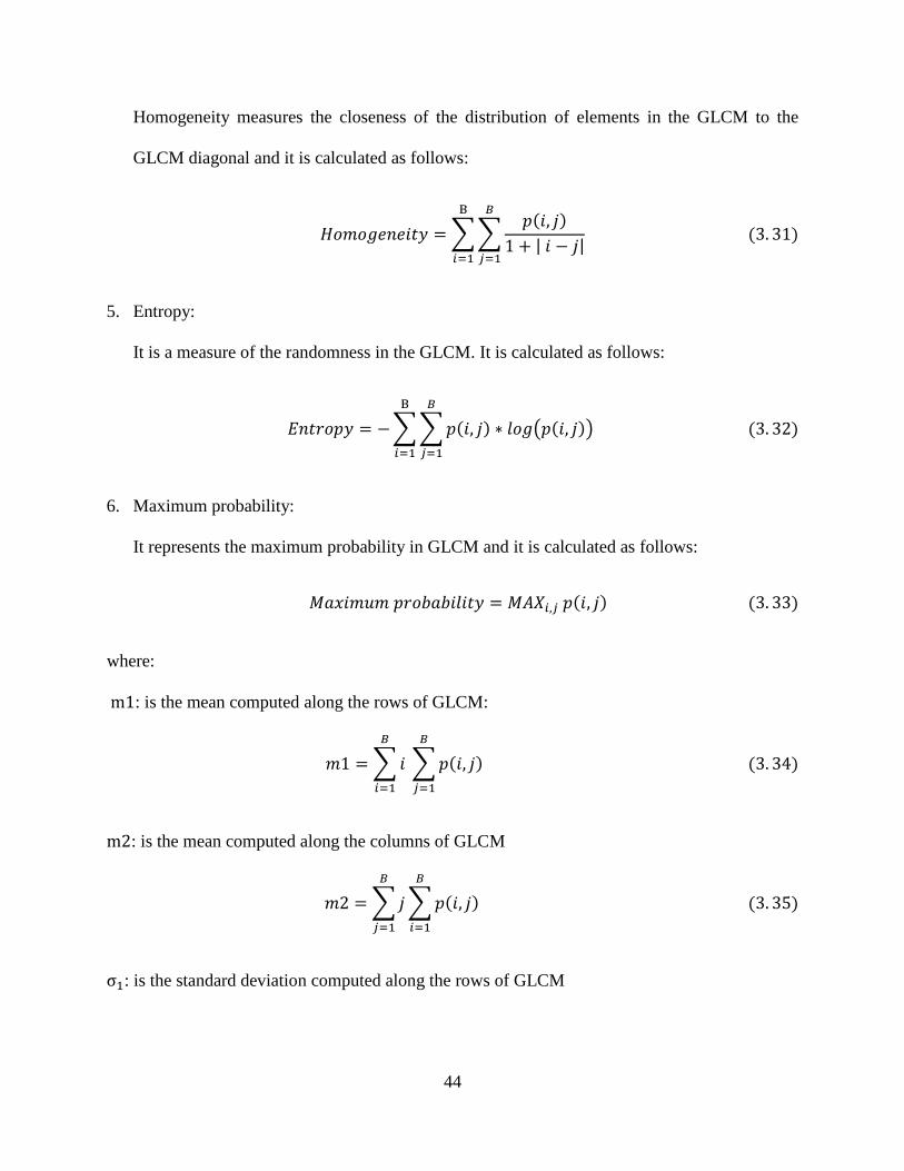
44
Homogeneity measures the closeness of the distribution of elements in the GLCM to the
GLCM diagonal and it is calculated as follows:
𝐻𝑜𝑚𝑜𝑔𝑒𝑛𝑒𝑖𝑡𝑦 = ∑∑𝑝(𝑖, 𝑗)
1 + | 𝑖 − 𝑗|
𝐵
𝑗=1
B
𝑖=1
(3. 31)
5. Entropy:
It is a measure of the randomness in the GLCM. It is calculated as follows:
𝐸𝑛𝑡𝑟𝑜𝑝𝑦 = −∑∑𝑝(𝑖, 𝑗) ∗ 𝑙𝑜𝑔(𝑝(𝑖, 𝑗))
𝐵
𝑗=1
B
𝑖=1
(3. 32)
6. Maximum probability:
It represents the maximum probability in GLCM and it is calculated as follows:
𝑀𝑎𝑥𝑖𝑚𝑢𝑚 𝑝𝑟𝑜𝑏𝑎𝑏𝑖𝑙𝑖𝑡𝑦 = 𝑀𝐴𝑋𝑖,𝑗 𝑝(𝑖, 𝑗) (3. 33)
where:
m1: is the mean computed along the rows of GLCM:
𝑚1 = ∑𝑖
𝐵
𝑖=1
∑𝑝(𝑖, 𝑗)
𝐵
𝑗=1
(3. 34)
m2: is the mean computed along the columns of GLCM
𝑚2 = ∑𝑗
𝐵
𝑗=1
∑𝑝(𝑖, 𝑗)
𝐵
𝑖=1
(3. 35)
σ1: is the standard deviation computed along the rows of GLCM

45
𝜎12 = ∑(𝑖 − 𝑚1)2
𝐵
𝑖=1
∑𝑝(𝑖, 𝑗)
𝐵
𝑗=1
(3. 36)
σ2: is the standard deviation computed along the row of GLCM
𝜎22 = ∑(𝑗 − 𝑚1)2
𝐵
𝑗=1
∑𝑝(𝑖, 𝑗)
𝐵
𝑖=1
(3. 37)
3.3.4 The Proposed Method for Feature Extraction
The steps below are applied to extract the significant features from the ROI of the MRI
brain images. These features are a combination of features generated using 2-D DWT and 2-D
Gabor filter followed by statistical calculation.
A. Initialization
➢ Giving a set of images 𝐼(𝑥, 𝑦)
➢ Set the number of level for the 2-D DWT (𝑙)
➢ Select a wavelet filter
ℎ0(𝑛): low pass filter coefficients
ℎ1(𝑛): high pass filter coefficients
➢ Set the values of the wavelength and orientation for Gabor filter
B. Extracting Features
For each image
➢ Step one: Calculate the first level wavelet coefficients (sub-band images) using equations 3.10
– 3.17

46
➢ Step two: Repeat step one for each level by setting 𝐿𝐿1 instead of 𝐼(𝑥, 𝑦) and 𝐿𝐿2 instead of
𝐿𝐿1 and so on.
➢ Step three: for each sub-band image, calculate:
a. The histogram of the image using equation (3.21)
b. The four first order statistics using equations (3.22 – 3.25)
c. The GLCM matrix using equations (3.26 and 3.27)
d. The six-second order statistics using equations (3.28 – 3.37)
➢ Step four: concatenate the features generated using the wavelet transform in a single vector.
The size of the vector is calculated according to the following formula:
(no. of wavelet
Features) = (
no. of levels
) ∗ (no. of
sub − bands) ∗ (
no. of statistical features
)
➢ Step five: generate 2-D Gabor filter kernels using equation (3.18) with the specified
wavelengths and orientations.
➢ Step six: convolve the input image (ROI) with the generated kernels using equation (3.19).
➢ Step seven: for each image resulted from the convolution, calculate the ten statistical features
as in step three.
➢ Step eight: concatenate the features generated using Gabor filter in a single vector, the
following formula determines the size of this vector:
(no. of GaborFeatures
) = (no. of
wavelengths) ∗ (
no. of orientations
) ∗ (no. of
statistical features)
➢ Step nine: concatenate the wavelets features and Gabor features to generate a single vector
which represents the total features.
➢ Step ten: repeat steps one to nine for each image.

47
3.4 Classification using Stacked Sparse Autoencoder and Softmax Classifier
The algorithm proposed for brain tumor classification is based on two types of neural
networks, the Sparse Autoencoder and the Softmax classifier. Thus, it is reasonable to start with a
brief introduction on the basic concept of the neural network. This section discusses the building
block design of the neural network and how this network is designed for multilayer perceptron and
trained using the backpropagation algorithm. Following this, the autoencoder is presented as a
special type of neural network designed for feature learning and how sparsity is imposed to
improve the performance of the basic autoencoder.
3.4.1 Introduction to Neural Network
A neural network is a machine designed to perform a task; the network model is stemmed
from the brain and it is usually implemented using electronic components or is simulated in
software on a digital computer. The main building block of a neural network is the neuron which
works as an information processing operation [65]. The basic form of the perceptron model shown
in fig. 3.10 is used to learn a decision function to recognize two classes.
Figure 3.10: A Nonlinear model of a neuron
∑ Activation
function
Wj1
Wj2
WjM
x1
x2
xM
vj
yj
b 1
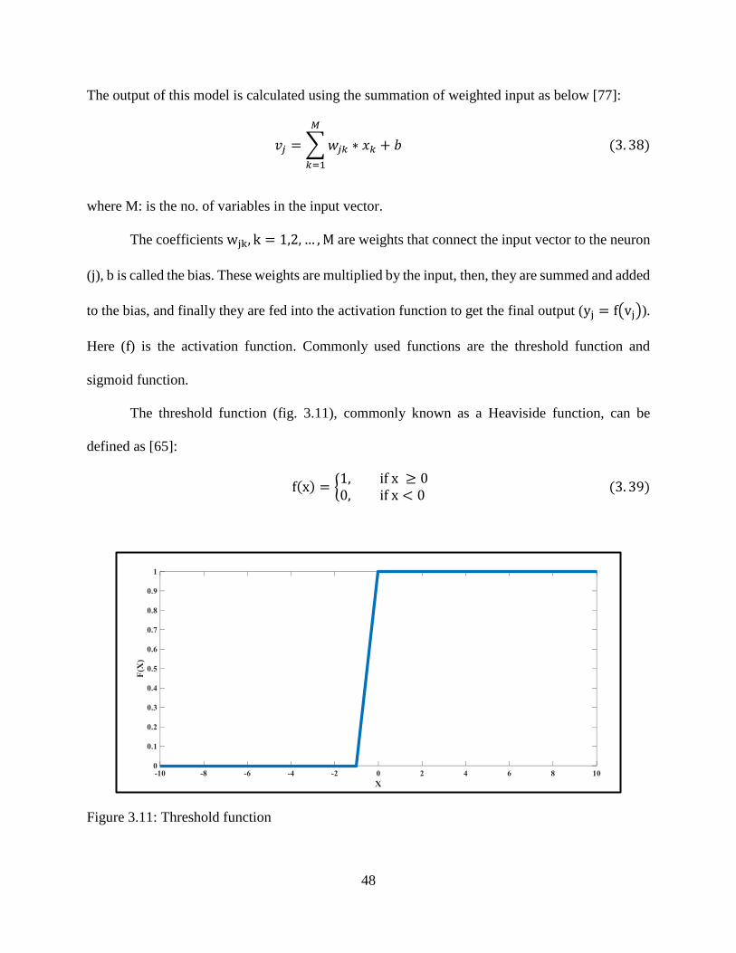
48
The output of this model is calculated using the summation of weighted input as below [77]:
𝑣𝑗 = ∑𝑤𝑗𝑘
𝑀
𝑘=1
∗ 𝑥𝑘 + 𝑏 (3. 38)
where M: is the no. of variables in the input vector.
The coefficients wjk, k = 1,2, … ,M are weights that connect the input vector to the neuron
(j), b is called the bias. These weights are multiplied by the input, then, they are summed and added
to the bias, and finally they are fed into the activation function to get the final output (yj = f(vj)).
Here (f) is the activation function. Commonly used functions are the threshold function and
sigmoid function.
The threshold function (fig. 3.11), commonly known as a Heaviside function, can be
defined as [65]:
f(x) = {1, if x ≥ 0 0, if x < 0
(3. 39)
Figure 3.11: Threshold function
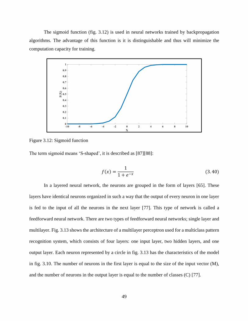
49
The sigmoid function (fig. 3.12) is used in neural networks trained by backpropagation
algorithms. The advantage of this function is it is distinguishable and thus will minimize the
computation capacity for training.
Figure 3.12: Sigmoid function
The term sigmoid means ‘S-shaped’, it is described as [87][88]:
𝑓(𝑥) =1
1 + 𝑒−𝑥 (3. 40)
In a layered neural network, the neurons are grouped in the form of layers [65]. These
layers have identical neurons organized in such a way that the output of every neuron in one layer
is fed to the input of all the neurons in the next layer [77]. This type of network is called a
feedforward neural network. There are two types of feedforward neural networks; single layer and
multilayer. Fig. 3.13 shows the architecture of a multilayer perceptron used for a multiclass pattern
recognition system, which consists of four layers: one input layer, two hidden layers, and one
output layer. Each neuron represented by a circle in fig. 3.13 has the characteristics of the model
in fig. 3.10. The number of neurons in the first layer is equal to the size of the input vector (M),
and the number of neurons in the output layer is equal to the number of classes (C) [77].

50
Figure 3.13: Architecture of multilayer neural network
For each layer (l), the output is calculated as [89]:
𝑣𝑗(𝑙+1) = ∑𝑤𝑗𝑘
(𝑙)
𝑁
𝑘=1
∗ 𝑥𝑘 + 𝑏𝑗(𝑙) (3. 41)
𝑦𝑗(𝑙+1) = 𝑓(𝑣𝑗
(𝑙+1)) (3. 42)
where N: is the no. of neurons in the hidden layer
For the first layer, yj(1) = xk, which is the kth element in the input vector (N=M), the
computation of this network is performed by calculating the activations in layer 2, then layer 3,
and so on using equations 3.41 and 3.42 in a feedforward manner [89].
3.4.2 Training Using Backpropagation Algorithm
The multilayer neural network is trained using a training set:
{X(i), R(i)}i=1S = {(X(1), D(1)), (X(2), D(2)), … , (X(S), D(S))}
where,
X(i): is the ith input vector of the training samples, (𝑋 = {𝑋1, 𝑋2, . . . , 𝑋𝑀}).
x1
x2
x3
y1
xM
y2
Input
layer
yC
Hidden layers
Output
layer
51
D(i): is the ith target vector (or labels for these samples)
S: is the number of training samples
The goal of training neural network is to minimize the cost function ℂ(𝑤) as a function of w. The
cost function is expressed as [19]:
ℂ = ∑ℇ(𝑖)
𝑆
𝑖=1
(3. 43)
Where ℇ is the error function.
There are two types of cost functions, least squares and cross-entropy cost functions. The
least squares cost function is the sum of square errors in the output neurons between the desired
response (𝑑(𝑖)) and the actual response (𝑦(𝑖)), it is described as [19]:
ℇ(𝑖) =1
2∑(𝑑𝑗(𝑖) − 𝑦𝑗(𝑖))
2𝑁𝐿
𝑗=1
(3. 44)
where 𝑁𝐿 is the no. of neurons in the last layer.
The cross-entropy function depends on the relative errors and not on the absolute errors;
therefore, it gives the same weight to small and large values. It is defined as [19]:
ℇ(𝑖) = ∑𝑑𝑗(𝑖) ∗ 𝑙𝑛 (𝑦𝑗(𝑖)) + (1 − 𝑑𝑗(𝑖)) ∗ 𝑙𝑛 (1 − (𝑦𝑗(𝑖))
𝑁𝐿
𝑗=1
(3. 45)
This minimization is carried out by first initializing the weight of the network with small
random values near zero, and then applying an optimization algorithm, such as the Gradient
Descent (GD) or the Conjugate Gradient (CG) algorithms [89]. The general gradient descent is an

52
optimization algorithm that is based on the least mean squares algorithm (LMS), it can be written
as [77], [90].
𝑤(𝑟 + 1) = 𝑤(𝑟) − 𝛼 ∗ [𝜕ℂ(𝑤)
𝜕𝑤]𝑊=𝑊(𝑟)
(3. 46)
Where,
w(r+1): is the new value of weight
r: is the iterative step
𝛼 > 0: is the learning rate,
The GD algorithm is robust to any changes in the initialization of the learning rate [90].
The learning rate is very important and plays a crucial role in the convergence of the algorithm. If
it is too small the weight corrections will be small, and the algorithm is converged slowly to the
optimum point. On the other hand, for a larger learning rate value, the convergence is impossible
since the algorithm may oscillate around the optimum value [19]. The correction Δwjk is applied
to the weight connecting neuron j to neuron k (k preceding j) and is defined by the delta rule [65]:
𝛥𝑤𝑗𝑘(𝑙)(𝑟) = 𝛼 ∗ ∑𝜌𝑗𝑘
(𝑙)
𝑆
𝑖=1
∗ 𝑦𝑗(𝑙−1) (3. 47)
where:
𝛥𝑤𝑗𝑘(𝑙)
(𝑟) = 𝑤𝑗𝑘(𝑙)(𝑟 + 1) − 𝑤𝑗𝑘
(𝑙)(𝑟): weight correction
𝜌𝑗(𝑙)
: the local gradient for neuron j at layer l
𝑦𝑗(𝑙−1)
: the output of neuron j at layer (l-1) that precedes layer l immediately
To avoid the instability and increase the rate of learning, delta rule is modified by including
a momentum term as follows [48]:
53
𝛥𝑤𝑗𝑘(𝑙)(𝑟) = 𝜇 ∗ 𝛥𝑤𝑗𝑘
(𝑙)(𝑟 − 1) + 𝛼 ∗ ∑𝜌𝑗(𝑙)
𝑆
𝑖=1
∗ 𝑦𝑗(𝑙−1) (3. 48)
where 𝜇 is the momentum, and the equation (3.48) is called the generalized delta rule.
“The conjugate-gradient method belongs to a class of second-order optimization methods
known collectively as conjugate-direction methods”. It is proposed to accelerate the slow rate of
convergence experienced by using the gradient descent method [65]. The correction term is
calculated as follows [19]:
𝛥𝑤𝑗𝑖(𝑙)(𝑟) = ℧(𝑟) + 𝜁(𝑟) ∗ 𝛥𝑤𝑗𝑖
(𝑙)(𝑟 − 1) (3. 49)
where:
℧(𝑟) = [𝜕ℂ(𝑤)
𝜕𝑤]𝑊=𝑊(𝑟)
(3. 50)
𝜁(𝑟) =℧𝑇(𝑟) ∗ ℧(𝑟)
℧𝑇(𝑟 − 1) ∗ ℧(𝑟 − 1), (𝐹𝑙𝑒𝑡𝑐ℎ𝑒𝑟 − 𝑅𝑒𝑒𝑣𝑒𝑠 𝐹𝑜𝑟𝑚𝑢𝑙𝑎) (3. 51)
𝜁(𝑟) =℧𝑇(𝑟) ∗ [℧(𝑟) − ℧(𝑟 − 1)]
℧𝑇(𝑟 − 1) ∗ ℧(𝑟 − 1), (𝑃𝑜𝑙𝑎𝑘 − 𝑅𝑖𝑏𝑖𝑒𝑟𝑒 𝐹𝑜𝑟𝑚𝑢𝑙𝑎) (3. 52)
Adjusting the weights in the output layer is simple since the desired output is known. The
problem is adjusting the weights in the hidden layers [77]. The backpropagation algorithm is
designed to train a multilayer neural network by computing the partial derivative of the cost
function with respect to the weight. In addition, the backpropagation algorithm is beneficial in
adjusting the weights in the hidden layer.

54
The following steps can be implemented to perform the backpropagation algorithm using
a training set {X(i), D(i)}, the input vector X(i) is applied to the input layer and the desired response
vector D(i) is presented to the output layer [19], [65]:
Initialization: Set the weights to small random values from a pseudo sequence random generator.
Forward computation: For each of the training input vector X:
➢ Calculate the input to the activation of the neuron (j) in layer (l+1) as:
𝑣𝑗(𝑙+1)(𝑖) = ∑𝑤𝑗𝑘
(𝑙)
𝑁
𝑘=1
(𝑖) ∗ 𝑦𝑗(𝑙)(𝑖) + 𝑏𝑗
(𝑙) (3. 53)
where yj(𝑙)(i) is the output of neuron j in the layer 𝑙 at sample i, and Wjk
(𝑙)(r) is the weight of neuron
j in layer l+1 that is fed from neuron k in layer 𝑙.
➢ Calculate the output of neuron j in layer l+1 as:
𝑦𝑗(𝑙+1)(𝑖) = 𝑓 (𝑣𝑗
(𝑙+1)(𝑖)) (3. 54)
If neuron j is in the first hidden layer set yj(1)(i) = xj(i), where xj(𝑖) is the jth element of the input
vector X(i).
➢ Compute the error signal as:
𝑒𝑗(𝑖) = 𝑑𝑗(𝑖) − 𝑦𝑗(𝐿)(𝑖) (3. 55)
Where, dj(i) is the jth element of the desired response vector D(i), and 𝑦𝑗(𝐿)
is the output of neuron
j in the output layer.
Backward Computation:
➢ Calculate the local gradients of the network as follows:
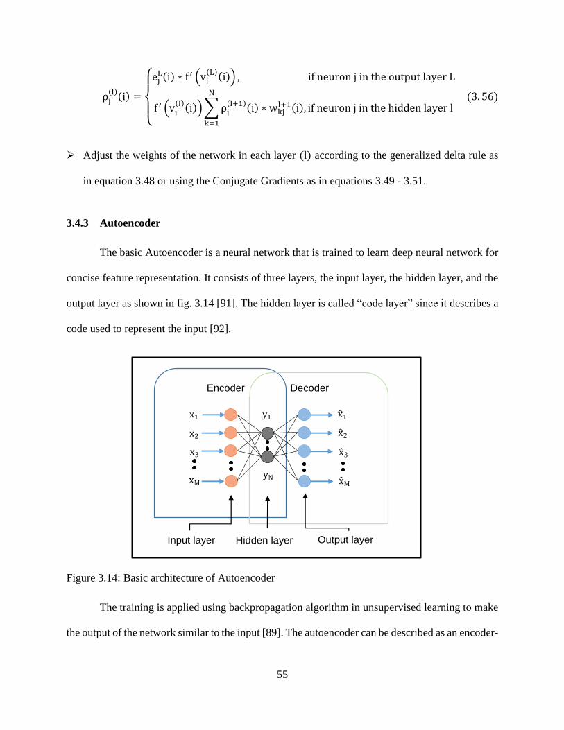
55
ρj(l)(i) =
{
ej
L(i) ∗ f ′ (vj(L)(i)) , if neuron j in the output layer L
f ′ (vj(l)(i))∑ρj
(l+1)(i)
N
k=1
∗ wkjl+1(i), if neuron j in the hidden layer l
(3. 56)
➢ Adjust the weights of the network in each layer (l) according to the generalized delta rule as
in equation 3.48 or using the Conjugate Gradients as in equations 3.49 - 3.51.
3.4.3 Autoencoder
The basic Autoencoder is a neural network that is trained to learn deep neural network for
concise feature representation. It consists of three layers, the input layer, the hidden layer, and the
output layer as shown in fig. 3.14 [91]. The hidden layer is called “code layer” since it describes a
code used to represent the input [92].
Figure 3.14: Basic architecture of Autoencoder
The training is applied using backpropagation algorithm in unsupervised learning to make
the output of the network similar to the input [89]. The autoencoder can be described as an encoder-
Encoder Decoder
x3
x1
x2
xM
x 1
x 2
x 3
x M
Input layer Hidden layer Output layer
y1
yN

56
decoder architecture where the encoder maps or encodes the input vector (X) into another vector
(Y) with less dimension.
Recall equations 3.41 and 3.42 the encoder part is expressed as [93]:
𝑣𝑗(2) = ∑𝑤𝑗𝑘
(1)
𝑀
𝑘=1
∗ 𝑥𝑘 + 𝑏𝑗(1) (3. 57)
𝑦𝑗(2) = 𝑓1(𝑣𝑗
(2)) (3. 58)
𝑤𝑗𝑘(1)
: the weight connection between neuron j in the hidden layer (layer 2) and neuron 𝑘 in the
input layer (layer 1) of the encoder networks
𝑏𝑗(2)
: the bias of neuron j
𝑓1: is the activation function of the encoder part
While the decoder network tries to reconstruct the original input vector from the encoded
representation and it is calculated as follows:
𝑣𝑘(3) = ∑𝑤𝑘𝑗
(2)
𝑁
𝑗=1
∗ 𝑦𝑗 + 𝑏𝑘(2) (3. 59)
𝑥 𝑗 = 𝑦𝑗(3) = 𝑓2(𝑣𝑘
(3)) (3. 60)
where,
X̂: the estimated vector
𝑓2: is the activation function of the decoder part
If the activation function of the encoder part is linear and the cost function is the mean
square error, then the autoencoder will learn to span the same subspace as the principal component
57
analysis (PCA). Furthermore, the autoencoder can learn a more powerful nonlinear generalization
of the PCA when the encoder and decoder functions are nonlinear [92].
The cost function of a basic autoencoder is the mean square error between the input and
the estimated input [89]. This is expressed as follows:
ℂ(𝑖) =1
𝑆∑∑(𝑥 𝑘(𝑖) − 𝑥𝑘(𝑖))
2𝑀
𝑘=1
𝑆
𝑖=1
(3. 61)
where M is the number of neurons in the input/output layer.
Autoencoders were utilized for dimensionality reduction or feature learning. In addition, it
is considered as a special case of feedforward neural networks and may be trained with the
backpropagation algorithm using the same techniques, such as the gradient descent algorithm.
Copying the input to the output is useless. The goal here is not the output of the decoder, but the
useful properties of the vector (Y). To generate useful features from the autoencoder, a constraint
is made on the vector (Y) to force its dimension to be less than that of the input vector (X).
Depending on the size of the input layer and hidden layer, the autoencoder can be divided into two
types. These types are the under complete autoencoder, whose hidden layer dimension is less than
the input dimension, and overcomplete autoencoder, where the size of the hidden layer is greater
than that of the input layer. Learning the under complete variables forces the autoencoder to take
advantage of the most salient features of the training data. Whereas with the overcomplete
variables, the autoencoder is unable to learn these useful features [92].
3.4.4 Sparse Autoencoder
In addition to the problem of learning the overcomplete autoencoder, the drawback of the
basic Autoencoder is the problem of inconsiderable solutions that affect the performance of the
58
network. One way to avoid this problem is to introduce a regularization function in the hidden
layer and control the firing of neurons in that layer. In this case, each neuron in the hidden layer
will fire to a small number of training examples or vectors [91]. In addition, the regularization
constraint will help the autoencoder to learn features even when the number of neurons in the
hidden layer is large compared with the input layer [89].
In the regularized autoencoder model, the loss function encourages the model to have some
properties such as “sparsity of the representation, smallness of the derivative of the representation,
and robustness to noise or to missing inputs”. Typically sparse autoencoders are used to learn
features for the classification task [92].
For training a sparse autoencoder, sparsity regularization can be added to the cost function
in equation (3.61) using two constraints:
1. Sparsity Regularization
A neuron in the hidden layer is active when its output is close to 1, and it is considered as
inactive when its output is close to 0. To force a neuron to be inactive most of the time, a sparsity
constraint is enforced on the neuron as [89]:
�̂�𝑗 = 𝜂 (3. 62)
where, �̂�𝑗: is the average activation of neuron in the hidden layer, and it is calculated as:
�̂�𝑗 =1
𝑆∑𝑓(∑(𝑤𝑗𝑘 ∗ 𝑥𝑘(𝑖))
𝑁
𝑘=1
+ 𝑏𝑗)
𝑆
𝑖=1
(3. 63)
Also, 𝜂 is the sparsity parameter (a small number close to 0).

59
The Kullback-Leibler divergence [94] is utilized here as a sparsity regularization term to
measure the difference between the average activation value of a neuron j (�̂�𝑗) and its desired value
𝜂. Sparsity regularization (SR) is calculated as follows [91], [95]:
𝑆𝑅 = ∑𝐾𝐿(𝜂
�̂�𝑗)
𝑁
𝑗=1
(3. 64)
𝐾𝐿 (𝜂
�̂�𝑗) = 𝜂 ∗ 𝑙𝑜𝑔 (
𝜂
�̂�𝑗) + (1 − 𝜂) ∗ 𝑙𝑜𝑔 (
1 − 𝜂
1 − �̂�𝑗) (3. 65)
where:
➢ N: is the number of neurons in the hidden layer
➢ 𝜂: is the sparsity parameter
Equation (3.65) states that a neuron is fired when the value of its output activation is high.
2. L2-weight Regularization
To prevent overfitting, L2-weight regularization or weight decay is introduced into the cost
function to decrease the magnitude of the weight. The weight decay is calculated as shown below
[89], [95]:
𝐿𝑅 =1
2∑∑ ∑(𝑊𝑗𝑖
(𝑙))2
𝑁𝑙+1
𝑗=1
𝑁𝑙
𝑖=1
𝐿−1
𝑙=1
(3. 66)
where:
➢ L: is the number of layers
➢ Nl, Nl+1: is the number of neurons in the layers l, l+1 respectively
As a result, the cost function of a sparse autoencoder will be [93]:
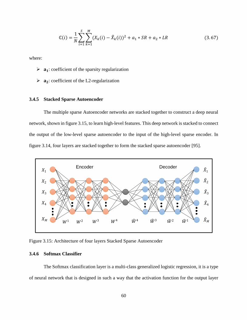
60
ℂ(𝑖) =1
𝑁∑∑(𝑋𝑘(𝑖) − �̂�𝑘(𝑖))
2
𝑀
𝑘=1
𝑆
𝑖=1
+ 𝑎1 ∗ 𝑆𝑅 + 𝑎2 ∗ 𝐿𝑅 (3. 67)
where:
➢ 𝐚𝟏: coefficient of the sparsity regularization
➢ 𝐚𝟐: coefficient of the L2-regularization
3.4.5 Stacked Sparse Autoencoder
The multiple sparse Autoencoder networks are stacked together to construct a deep neural
network, shown in figure 3.15, to learn high-level features. This deep network is stacked to connect
the output of the low-level sparse autoencoder to the input of the high-level sparse encoder. In
figure 3.14, four layers are stacked together to form the stacked sparse autoencoder [95].
Figure 3.15: Architecture of four layers Stacked Sparse Autoencoder
3.4.6 Softmax Classifier
The Softmax classification layer is a multi-class generalized logistic regression, it is a type
of neural network that is designed in such a way that the activation function for the output layer
Encoder Decoder 𝑋1
𝑋4
𝑋2
𝑋3
𝑋𝑀
�̂�1
�̂�2
�̂�3
�̂�4
�̂�𝑀 𝑊1 �̂�1 �̂�2
Input layer Hidden layers Output layer
𝑊2 𝑊3 𝑊4 �̂�3 �̂�4
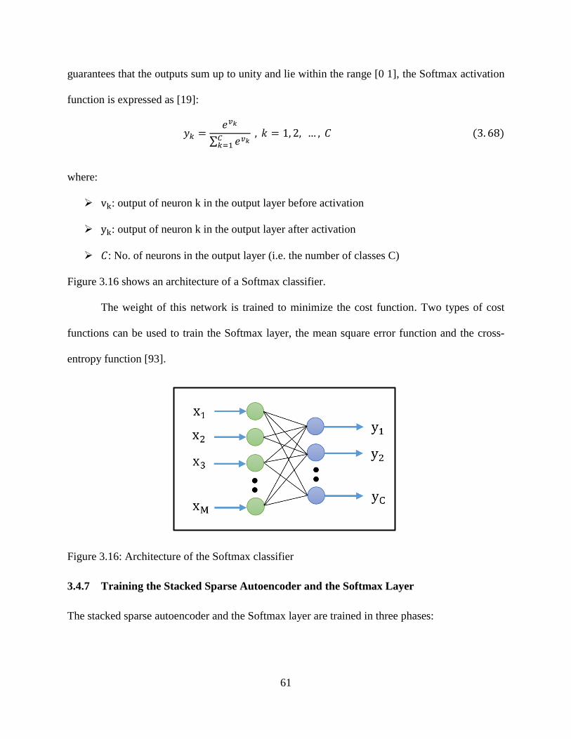
61
guarantees that the outputs sum up to unity and lie within the range [0 1], the Softmax activation
function is expressed as [19]:
𝑦𝑘 =𝑒𝑣𝑘
∑ 𝑒𝑣𝑘𝐶𝑘=1
, 𝑘 = 1, 2, … , 𝐶 (3. 68)
where:
➢ vk: output of neuron k in the output layer before activation
➢ yk: output of neuron k in the output layer after activation
➢ 𝐶: No. of neurons in the output layer (i.e. the number of classes C)
Figure 3.16 shows an architecture of a Softmax classifier.
The weight of this network is trained to minimize the cost function. Two types of cost
functions can be used to train the Softmax layer, the mean square error function and the cross-
entropy function [93].
Figure 3.16: Architecture of the Softmax classifier
3.4.7 Training the Stacked Sparse Autoencoder and the Softmax Layer
The stacked sparse autoencoder and the Softmax layer are trained in three phases:

62
I. Phase one: in this phase, the autoencoder is trained using the backpropagation algorithm to
optimize the cost function in an unsupervised manner (which means no labeled data is
needed).
The KL divergence term in the cost function can be added in the calculation of local gradients in
the hidden layer (layer 2) as follows [89]:
𝜌𝑗(2) = 𝑓′ (𝑣𝑗
(𝑙)(𝑖))∑𝜌𝑗(3)(𝑖)
𝑁
𝑘=1
∗ 𝑤𝑘𝑗3 (𝑖) + 𝑎1 ∗ (−
𝜂
�̂�𝑗+
1 − 𝜂
1 − �̂�𝑗 ) (3. 69)
The following steps are applied to describe phase one using a training set {X(i), D(i)}.
A. Initialization:
1. Set the weights to small random values from a pseudo sequence random generator.
2. Set the values of sparsity regularization and L2-weight regularization coefficients (a1 and
a2).
3. Select the number of autoencoder networks and the number of neurons in each network.
4. Assign the max number of iterations.
B. Forward Computations:
For each iteration, calculate:
1. The output of the encoder part of the first autoencoder using equations 3.57 and 3.58.
2. The output of the decoder part of the first autoencoder using equations 3.59 and 3.60
3. The error signal (ejL(i)) as follows:
ejL(i) = (𝑋𝑗(𝑖) − �̂�𝑗(𝑖))
2 + 𝑎1 ∗ 𝑆𝑅 + 𝑎2 ∗ 𝐿𝑅
C. Backward Computations:
For each iteration:

63
➢ Calculate the gradient as follows:
ρj(l)(i) =
{
ej
L(i) ∗ f ′ (vj(L)(i)) , if neuron j in the output layer L
f ′ (vj(l)(i))∑ρj
(l+1)(i)
N
k=1
∗ wkjl+1(i) + a1 ∗ (−
η
η j+
1 − η
1 − η j ) , for hidden layer
➢ Update the weight of the autoencoder network using Conjugate Gradient algorithm
equations 3.49, 3.50, and 3.51.
➢ Calculate the output of the encoder part of the first autoencoder after training using
equations 3.57 and 3.58.
➢ Repeat the forward and backward computations steps for the next autoencoder by making
the output of the first encoder part as the input vector.
II. Phase two: The Softmax classifier is trained in a supervised learning method using the
backpropagation algorithm described in section 3.4.2 with the cross-entropy cost function.
III. Phase three: After training the autoencoder, the encoder part will be separated and
combined with the Softmax classifier by connecting the output of the last encoder to the
input of the Softmax layer to generate a multilayer deep neural network as shown in fig.
3.17. The deep network is trained by fine-tuning its weights using the backpropagation
algorithm. The model in fig. 3.17 comprises from three layers stacked sparse autoencoder
and the Softmax layer; the input layer with size M, two hidden layers with size n1and n2,
respectively and the Softmax layer with size C.
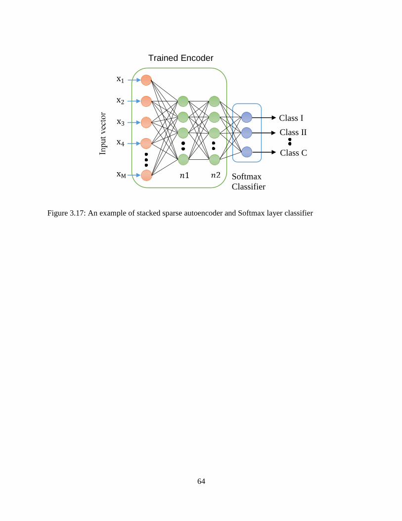
64
Figure 3.17: An example of stacked sparse autoencoder and Softmax layer classifier
Trained Encoder
x1
x4
x2
x3
xM 𝑛1 Softmax
Classifier
𝑛2
Class I
Class II
Class C
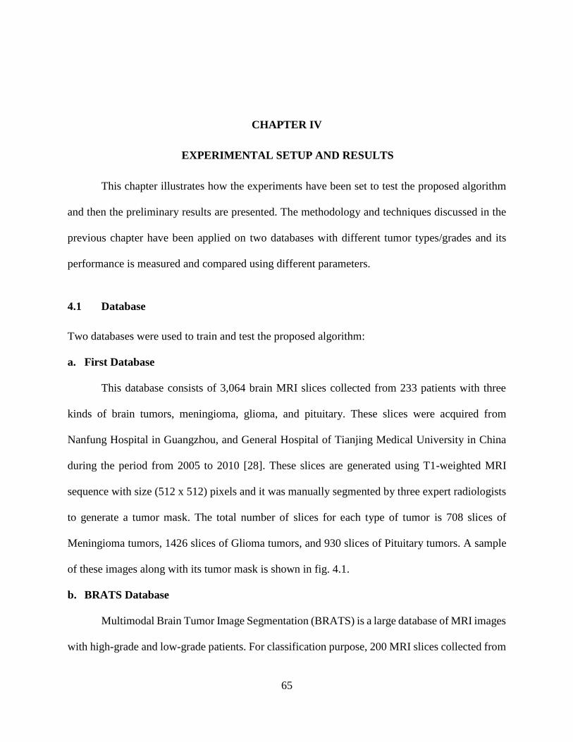
65
CHAPTER IV
4.EXPERIMENTAL SETUP AND RESULTS
This chapter illustrates how the experiments have been set to test the proposed algorithm
and then the preliminary results are presented. The methodology and techniques discussed in the
previous chapter have been applied on two databases with different tumor types/grades and its
performance is measured and compared using different parameters.
4.1 Database
Two databases were used to train and test the proposed algorithm:
a. First Database
This database consists of 3,064 brain MRI slices collected from 233 patients with three
kinds of brain tumors, meningioma, glioma, and pituitary. These slices were acquired from
Nanfung Hospital in Guangzhou, and General Hospital of Tianjing Medical University in China
during the period from 2005 to 2010 [28]. These slices are generated using T1-weighted MRI
sequence with size (512 x 512) pixels and it was manually segmented by three expert radiologists
to generate a tumor mask. The total number of slices for each type of tumor is 708 slices of
Meningioma tumors, 1426 slices of Glioma tumors, and 930 slices of Pituitary tumors. A sample
of these images along with its tumor mask is shown in fig. 4.1.
b. BRATS Database
Multimodal Brain Tumor Image Segmentation (BRATS) is a large database of MRI images
with high-grade and low-grade patients. For classification purpose, 200 MRI slices collected from
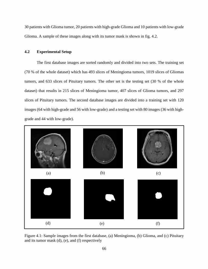
66
30 patients with Glioma tumor, 20 patients with high-grade Glioma and 10 patients with low-grade
Glioma. A sample of these images along with its tumor mask is shown in fig. 4.2.
4.2 Experimental Setup
The first database images are sorted randomly and divided into two sets. The training set
(70 % of the whole dataset) which has 493 slices of Meningioma tumors, 1019 slices of Gliomas
tumors, and 633 slices of Pituitary tumors. The other set is the testing set (30 % of the whole
dataset) that results in 215 slices of Meningioma tumor, 407 slices of Glioma tumors, and 297
slices of Pituitary tumors. The second database images are divided into a training set with 120
images (64 with high-grade and 56 with low-grade) and a testing set with 80 images (36 with high-
grade and 44 with low-grade).
Figure 4.1: Sample images from the first database, (a) Meningioma, (b) Glioma, and (c) Pituitary
and its tumor mask (d), (e), and (f) respectively
(a) (b) (c)
(d) (e) (f)
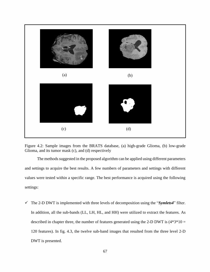
67
Figure 4.2: Sample images from the BRATS database, (a) high-grade Glioma, (b) low-grade
Glioma, and its tumor mask (c), and (d) respectively
The methods suggested in the proposed algorithm can be applied using different parameters
and settings to acquire the best results. A few numbers of parameters and settings with different
values were tested within a specific range. The best performance is acquired using the following
settings:
✓ The 2-D DWT is implemented with three levels of decomposition using the “Symlets4” filter.
In addition, all the sub-bands (LL, LH, HL, and HH) were utilized to extract the features. As
described in chapter three, the number of features generated using the 2-D DWT is (4*3*10 =
120 features). In fig. 4.3, the twelve sub-band images that resulted from the three level 2-D
DWT is presented.
(a) (b)
(c) (d)

68
Figure 4.3: Image decomposition using three levels of the 2-D DWT, the input image is an MRI
with a Meningioma tumor.
The input image is a slice of meningioma tumor. Its size is (512 x 512) pixels while the
size of tumor is (115 x 106) pixels, after decomposition, the size of first level sub-bands (i.e. LL1,
LH1, HL1, and HH1) will be (61 x 56) pixels (the first row in fig. 4.3), this change in size is the
result of subsampling of 2 of the DWT. Similarly, the size of second level sub-bands will be (34 x
31) pixels and the size of the third level sub-bands will be (20 x 19).
(a) (b)
(LL1) (LH1) (HL1)
(LL2) (LH2) (HH2)
(LL3)
(HH1)
(HH3) (HL3)
(HL2)
(LH3)

69
Figure 4.4: Visualization of images resulted from the 2-D Gabor filter with three values of
wavelengths and five values of orientations, (a) the original image, (b) its tumor mask, numbers in
brackets are (wavelength, orientation)
✓ The 2-D Gabor filter is applied on each image with three wavelengths (2, 4, and 8) while the
values of the orientations are (0°,45°, 90°, 135°, and 180°) to generate fifteen different images.
For each image the ten statistical values were applied resulting in 150 features. As shown in
(a) (b)
(2, 0°) (2, 45°) (2, 90°) (2, 135°) (2, 180°)
(4, 0°) (4, 45°) (4, 135°) (4, 180°)
(8, 0°) (8, 45°) (8, 90°) (8, 135°) (8, 180°)
(4, 90°)
70
fig. 4.4, fifteen different images represent the implementation of the 2-D Gabor filter on MRI
slices with Meningioma tumors.
✓ The classifier model consists of two types of neural network, the Stacked Sparse Autoencoder
(SSAE) and the Softmax classifier (SM). The SSAE comprises of four layers, the input layer,
two hidden layers, and an output layer. The number of features generated using a combination
of wavelet and Gabor filter is (120 + 150 = 270 features). As a result, the size of the input
and output layers is the same as the input features or equal to 270 neurons. The size of the first
hidden layer is set to 150 neurons, while the size of the second hidden size is set to 75 neurons.
The sparsity regularization coefficient is set to 1, and the L2-weight regularization coefficient
is set to 0.001. the SM classifier has two layers; an input layer with the size of 75 neurons (the
same as the second hidden layer) and an output layer with the size of 3 neurons (the number
of classes). For both networks, SSAE and SM, the conjugate gradient method is used for
optimization the cross-entropy cost function.
4.3 Performance Analysis
Measuring the performance of the proposed algorithm is based on the performance of the
classifier model that is determined using the labels given in the database. This can be done by
applying a set of examples to the classifier and measuring the number of errors the classifier has
made. There are four fundamental outcomes that are used to test the classifier [96];
1. True Positive: the classifier recognizes the positive example correctly.
2. True Negative: the classifier recognizes the negative example correctly.
3. False Negative: the classifier incorrectly recognizes the positive example as negative.
4. False Positive: the classifier incorrectly recognizes the negative example as positive.

71
In the case of brain tumor classification with multiclass, these quantities should be
calculated separately for each type of tumor. Furthermore, the positive case here is that the output
of the classifier is the tumor while the negative case is the non-tumor output.
If the classifier is applied to the whole dataset, with known real classes, these four outcomes
will be counted according to the number of times of occurrence. Here NTP is the number of true
positives, NTN is the number of true negatives, NFP is the number of false positives, and NFN is the
number of false negatives. The calculation of the performance of the classifier is based on these
numbers [96].
The performance of the proposed algorithm is measured using three criteria [96]:
1. Accuracy: is the frequency of correct classifications made by the classifier over a given set of
examples, it is calculated as:
Accuracy =𝑁𝑇𝑃 + 𝑁𝑇𝑁
𝑁𝐹𝑃 + 𝑁𝐹𝑁 + 𝑁𝑇𝑃 + 𝑁𝑇𝑁 (4.1)
2. Sensitivity: is the probability that a positive example will be correctly recognized by the
classifier, its formula is:
Sensitivity =𝑁𝑇𝑃
𝑁𝐹𝑁 + 𝑁𝑇𝑃 (4.2)
3. Specificity: is the probability that a negative example will be correctly recognized by the
classifier, its formula is:
Specificity =𝑁𝑇𝑁
𝑁𝐹𝑃 + 𝑁𝑇𝑁 (4.3)
Sensitivity and specificity are widely used measurements when applying machine learning to
medical data.
72
Receiver operating characteristics (ROC) is defined as a trade-off visualization between a
pair of criteria such, as sensitivity and specificity, in the plane spanned by the two measures [97].
In biomedical informatics research, ROC curves are frequently used to evaluate classification and
prediction models for decision support, diagnosis, and prognosis. Furthermore, ROC curves are
utilized to test the model accuracy and its ability to discriminate between positive and negative
cases. The full area under the ROC curve is defined as the average sensitivity for all values of
specificity or the average specificity for all values of sensitivity [98].
4.4 Simulation Results
This section describes some of the simulation results obtained from applying the proposed
algorithm to the database. These results are measured in terms of accuracy, sensitivity, and
specificity with different parameter settings.
4.4.1 Statistical Features Obtained from Wavelet Transform and Gabor Filter
Feature extraction is the most significant part of the proposed algorithm since it captures
the salient information from the ROI image to be ready for classification. As stated in chapter
three, these features are extracted using three techniques: 2-D DWT, Gabor filter, and statistical
calculation. The decomposition of the image using the 2-D DWT generates 12 different images.
Ten statistical features (mean, variance, skewness, kurtosis, contrast, correlation, energy,
homogeneity, maximum probability, and entropy) are extracted from each image. Table 4.1 lists
the statistical features extracted from three ROI images with different tumor types (Meningioma,
Glioma, and Pituitary) for the third level of the 2-D DWT.
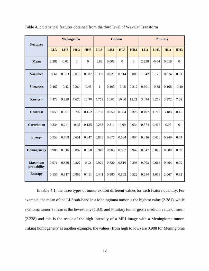
73
Table 4.1: Statistical features obtained from the third level of Wavelet Transform
Features
Meningioma Glioma Pituitary
LL3 LH3 HL3 HH3 LL3 LH3 HL3 HH3 LL3 LH3 HL3 HH3
Mean 2.381 -0.01 0 0 1.83 0.002 0 0 2.238 -0.04 0.019 0
Variance 0.661 0.023 0.018 0.007 0.399 0.021 0.014 0.008 1.042 0.125 0.074 0.01
Skewness 0.467 -0.42 0.264 -0.48 1 0.103 -0.18 0.212 0.601 -0.38 0.168 -0.40
Kurtosis 2.472 9.898 7.678 13.38 4.753 10.61 10.00 12.21 3.074 6.259 3.372 7.09
Contrast 0.059 0.591 0.702 0.152 0.732 0.650 0.594 0.326 0.497 1.719 3.183 0.45
Correlation 0.334 0.241 -0.05 0.135 0.283 0.311 -0.09 0.034 0.574 0.468 -0.07 0
Energy 0.953 0.708 0.651 0.847 0.855 0.677 0.664 0.804 0.816 0.450 0.249 0.64
Homogeneity 0.988 0.916 0.887 0.958 0.949 0.903 0.887 0.942 0.947 0.823 0.680 0.89
Maximum
probability
0.976 0.839 0.802 0.92 0.924 0.820 0.810 0.895 0.903 0.663 0.464 0.79
Entropy 0.157 0.817 0.865 0.411 0.441 0.880 0.802 0.522 0.554 1.613 2.067 0.82
In table 4.1, the three types of tumor exhibit different values for each feature quantity. For
example, the mean of the LL3 sub-band in a Meningioma tumor is the highest value (2.381), while
a Glioma tumor’s mean is the lowest one (1.83), and Pituitary tumor gets a medium value of mean
(2.238) and this is the result of the high intensity of a MRI image with a Meningioma tumor.
Taking homogeneity as another example, the values (from high to low) are 0.988 for Meningioma
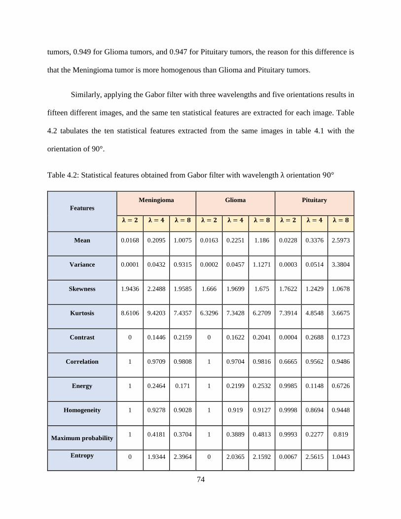
74
tumors, 0.949 for Glioma tumors, and 0.947 for Pituitary tumors, the reason for this difference is
that the Meningioma tumor is more homogenous than Glioma and Pituitary tumors.
Similarly, applying the Gabor filter with three wavelengths and five orientations results in
fifteen different images, and the same ten statistical features are extracted for each image. Table
4.2 tabulates the ten statistical features extracted from the same images in table 4.1 with the
orientation of 90°.
Table 4.2: Statistical features obtained from Gabor filter with wavelength λ orientation 90°
Features
Meningioma Glioma Pituitary
𝛌 = 𝟐 𝛌 = 𝟒 𝛌 = 𝟖 𝛌 = 𝟐 𝛌 = 𝟒 𝛌 = 𝟖 𝛌 = 𝟐 𝛌 = 𝟒 𝛌 = 𝟖
Mean 0.0168 0.2095 1.0075 0.0163 0.2251 1.186 0.0228 0.3376 2.5973
Variance 0.0001 0.0432 0.9315 0.0002 0.0457 1.1271 0.0003 0.0514 3.3804
Skewness 1.9436 2.2488 1.9585 1.666 1.9699 1.675 1.7622 1.2429 1.0678
Kurtosis 8.6106 9.4203 7.4357 6.3296 7.3428 6.2709 7.3914 4.8548 3.6675
Contrast 0 0.1446 0.2159 0 0.1622 0.2041 0.0004 0.2688 0.1723
Correlation 1 0.9709 0.9808 1 0.9704 0.9816 0.6665 0.9562 0.9486
Energy 1 0.2464 0.171 1 0.2199 0.2532 0.9985 0.1148 0.6726
Homogeneity 1 0.9278 0.9028 1 0.919 0.9127 0.9998 0.8694 0.9448
Maximum probability 1 0.4181 0.3704 1 0.3889 0.4813 0.9993 0.2277 0.819
Entropy 0 1.9344 2.3964 0 2.0365 2.1592 0.0067 2.5615 1.0443
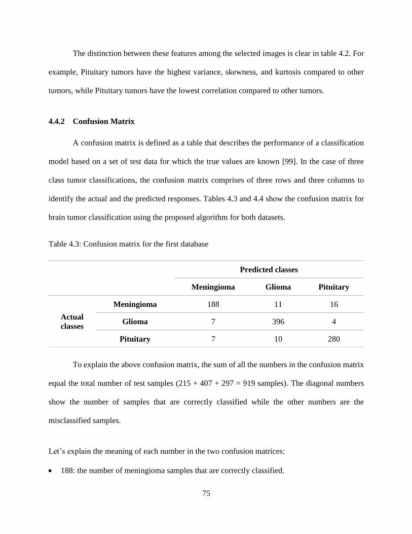
75
The distinction between these features among the selected images is clear in table 4.2. For
example, Pituitary tumors have the highest variance, skewness, and kurtosis compared to other
tumors, while Pituitary tumors have the lowest correlation compared to other tumors.
4.4.2 Confusion Matrix
A confusion matrix is defined as a table that describes the performance of a classification
model based on a set of test data for which the true values are known [99]. In the case of three
class tumor classifications, the confusion matrix comprises of three rows and three columns to
identify the actual and the predicted responses. Tables 4.3 and 4.4 show the confusion matrix for
brain tumor classification using the proposed algorithm for both datasets.
Table 4.3: Confusion matrix for the first database
To explain the above confusion matrix, the sum of all the numbers in the confusion matrix
equal the total number of test samples (215 + 407 + 297 = 919 samples). The diagonal numbers
show the number of samples that are correctly classified while the other numbers are the
misclassified samples.
Let’s explain the meaning of each number in the two confusion matrices:
• 188: the number of meningioma samples that are correctly classified.
Predicted classes
Meningioma Glioma Pituitary
Actual
classes
Meningioma 188 11 16
Glioma 7 396 4
Pituitary 7 10 280

76
• 11: the number of Meningioma tumor samples that are classified as Glioma tumors.
• 16: the number of Meningioma tumor samples that are classified as a Pituitary tumor.
• 7 (2nd row): the number of Glioma tumor samples that are classified as meningioma.
• 396: the number of Gliomas samples that are classified correctly.
• 4: the number of Gliomas samples that are classified as Pituitary tumors.
• 7 (third row): the number of Pituitary tumor samples that are classified as Meningioma tumors.
• 10: the number of Pituitary tumor samples that are classified as Gliomas.
• 280: the number of Pituitary tumor samples that are classified correctly
Table 4.4: Confusion matrix for the BRATS database
Predicted classes
High-grade Low-grade
Actual
classes
High-grade 36 0
Low-grade 1 43
In table 4.4, 36 slices with high-grade Glioma and 43 slices with low-grade Glioma are correctly
classified, while one slice with low-grade is incorrectly classified as high-grade.
Based on the information in the confusion matrices the accuracy, sensitivity, and specificity
can be determined for each type of tumor. First, it is better to determine the four outcomes
represented by true positive (TP), true negative (TN), false positive (FP), and false negative (FN).
Table 4.5 explains the values of these outcomes, while table 4.6 shows results for performance
evaluation for each tumor type.
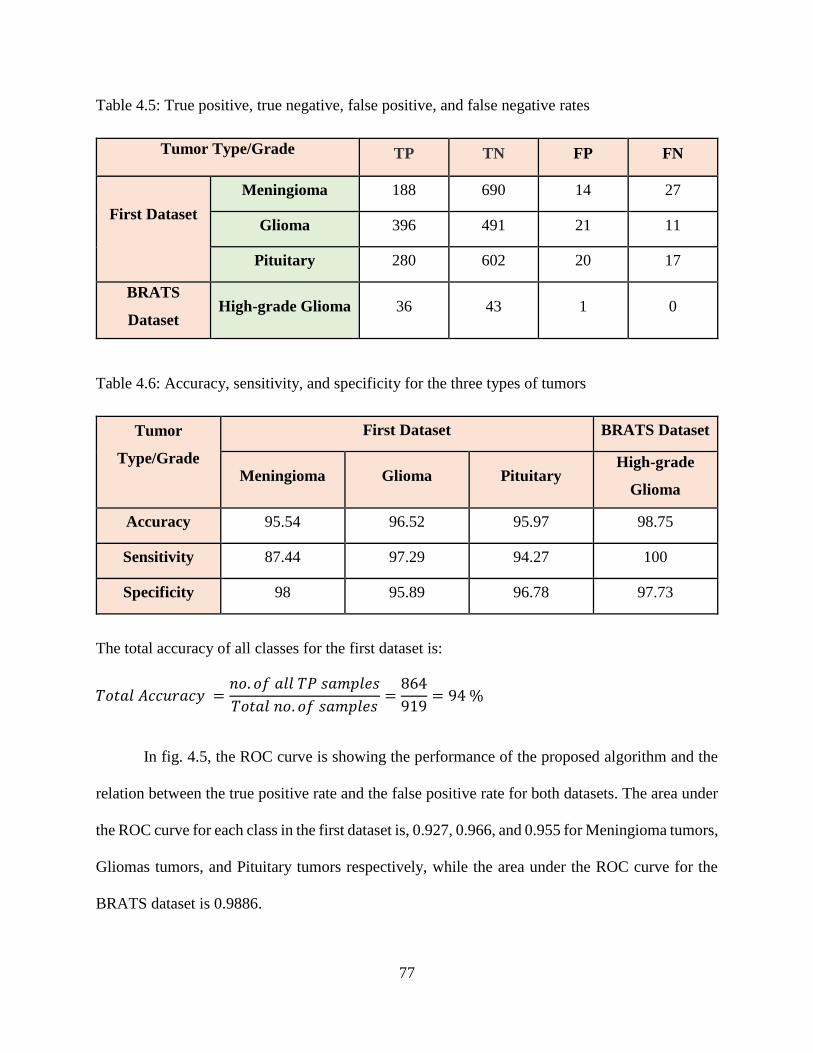
77
Table 4.5: True positive, true negative, false positive, and false negative rates
Tumor Type/Grade TP TN FP FN
First Dataset
Meningioma 188 690 14 27
Glioma 396 491 21 11
Pituitary 280 602 20 17
BRATS
Dataset High-grade Glioma 36 43 1 0
Table 4.6: Accuracy, sensitivity, and specificity for the three types of tumors
Tumor
Type/Grade
First Dataset BRATS Dataset
Meningioma Glioma Pituitary High-grade
Glioma
Accuracy 95.54 96.52 95.97 98.75
Sensitivity 87.44 97.29 94.27 100
Specificity 98 95.89 96.78 97.73
The total accuracy of all classes for the first dataset is:
𝑇𝑜𝑡𝑎𝑙 𝐴𝑐𝑐𝑢𝑟𝑎𝑐𝑦 =𝑛𝑜. 𝑜𝑓 𝑎𝑙𝑙 𝑇𝑃 𝑠𝑎𝑚𝑝𝑙𝑒𝑠
𝑇𝑜𝑡𝑎𝑙 𝑛𝑜. 𝑜𝑓 𝑠𝑎𝑚𝑝𝑙𝑒𝑠=
864
919= 94 %
In fig. 4.5, the ROC curve is showing the performance of the proposed algorithm and the
relation between the true positive rate and the false positive rate for both datasets. The area under
the ROC curve for each class in the first dataset is, 0.927, 0.966, and 0.955 for Meningioma tumors,
Gliomas tumors, and Pituitary tumors respectively, while the area under the ROC curve for the
BRATS dataset is 0.9886.

78
(a) (b)
Figure 4.5: ROC Curve for the classification model, (a) first dataset, (b) BRATS dataset
4.4.3 Wavelet Features
The 2-D DWT is used for extracting features with the Gabor filter. The number of
transformation levels and the type of filter determine the characteristics of the wavelet coefficients
that result from this transformation. To examine the effect of the wavelet filter type on the
performance of the proposed algorithm, different kinds of wavelet filters have been utilized in this
algorithm. These filters are: Haar, Daubechies 2, Coiflets1, Coiflets2, Coiflets3, Symlets2,
Symlets4, Symlets8, and Discrete Meyer. Fig. 4.6 summarizes the accuracy of the proposed
algorithm for each type of wavelet filters. In this figure, ‘Symlets4’ exhibits the highest accuracy
while ‘Symlets2’ shows the lowest accuracy. Selection of the filter for feature extraction is
determined by the type of problem or the input data.
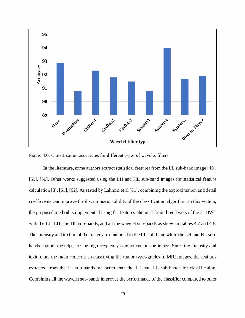
79
Figure 4.6: Classification accuracies for different types of wavelet filters
In the literature, some authors extract statistical features from the LL sub-band image [40],
[59], [60]. Other works suggested using the LH and HL sub-band images for statistical feature
calculation [8], [61], [62]. As stated by Lahmiri et al [61], combining the approximation and detail
coefficients can improve the discrimination ability of the classification algorithm. In this section,
the proposed method is implemented using the features obtained from three levels of the 2- DWT
with the LL, LH, and HL sub-bands, and all the wavelet sub-bands as shown in tables 4.7 and 4.8.
The intensity and texture of the image are contained in the LL sub-band while the LH and HL sub-
bands capture the edges or the high frequency components of the image. Since the intensity and
texture are the main concerns in classifying the tumor types/grades in MRI images, the features
extracted from the LL sub-bands are better than the LH and HL sub-bands for classification.
Combining all the wavelet sub-bands improves the performance of the classifier compared to other
89
90
91
92
93
94
95A
ccu
racy
Wavelet filter type
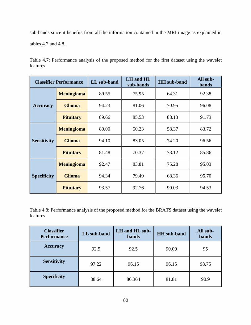
80
sub-bands since it benefits from all the information contained in the MRI image as explained in
tables 4.7 and 4.8.
Table 4.7: Performance analysis of the proposed method for the first dataset using the wavelet
features
Classifier Performance LL sub-band LH and HL
sub-bands HH sub-band
All sub-
bands
Accuracy
Meningioma 89.55 75.95 64.31 92.38
Glioma 94.23 81.06 70.95 96.08
Pituitary 89.66 85.53 88.13 91.73
Sensitivity
Meningioma 80.00 50.23 58.37 83.72
Glioma 94.10 83.05 74.20 96.56
Pituitary 81.48 70.37 73.12 85.86
Specificity
Meningioma 92.47 83.81 75.28 95.03
Glioma 94.34 79.49 68.36 95.70
Pituitary 93.57 92.76 90.03 94.53
Table 4.8: Performance analysis of the proposed method for the BRATS dataset using the wavelet
features
Classifier
Performance LL sub-band
LH and HL sub-
bands HH sub-band
All sub-
bands
Accuracy
92.5 92.5 90.00 95
Sensitivity
97.22 96.15 96.15 98.75
Specificity
88.64 86.364 81.81 90.9

81
4.4.4 Gabor Features
In section 3.3.2, two approaches were presented to describe Gabor features. The first
approach is the Gabor filter that is implemented by a convolution between the input image and the
2-D Gabor function (equation 3.19). The second one is the Gabor energy approach, which is
applied by combining a symmetric and an antisymmetric kernel filter in each image (equation
3.20). In this section, a comparison is carried out to study the effect of Gabor filter features for
both approaches and the results are described in tables 4.9 and 4.10.
Table 4.9: Performance analysis of the proposed algorithm for the first dataset with Gabor and
Gabor energy features
Classifier Performance Gabor Filter Features Gabor Energy Features
Accuracy
Meningioma 93.03 90.86
Glioma 93.14 91.84
Pituitary 94.23 92.49
Sensitivity
Meningioma 85.12 80.46
Glioma 93.36 92.38
Pituitary 89.56 86.19
Specificity
Meningioma 95.45 94.03
Glioma 92.97 91.41
Pituitary 96.46 95.5
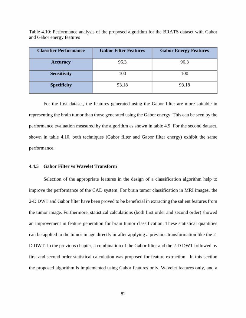
82
Table 4.10: Performance analysis of the proposed algorithm for the BRATS dataset with Gabor
and Gabor energy features
Classifier Performance Gabor Filter Features Gabor Energy Features
Accuracy 96.3 96.3
Sensitivity 100 100
Specificity 93.18 93.18
For the first dataset, the features generated using the Gabor filter are more suitable in
representing the brain tumor than those generated using the Gabor energy. This can be seen by the
performance evaluation measured by the algorithm as shown in table 4.9. For the second dataset,
shown in table 4.10, both techniques (Gabor filter and Gabor filter energy) exhibit the same
performance.
4.4.5 Gabor Filter vs Wavelet Transform
Selection of the appropriate features in the design of a classification algorithm help to
improve the performance of the CAD system. For brain tumor classification in MRI images, the
2-D DWT and Gabor filter have been proved to be beneficial in extracting the salient features from
the tumor image. Furthermore, statistical calculations (both first order and second order) showed
an improvement in feature generation for brain tumor classification. These statistical quantities
can be applied to the tumor image directly or after applying a previous transformation like the 2-
D DWT. In the previous chapter, a combination of the Gabor filter and the 2-D DWT followed by
first and second order statistical calculation was proposed for feature extraction. In this section
the proposed algorithm is implemented using Gabor features only, Wavelet features only, and a
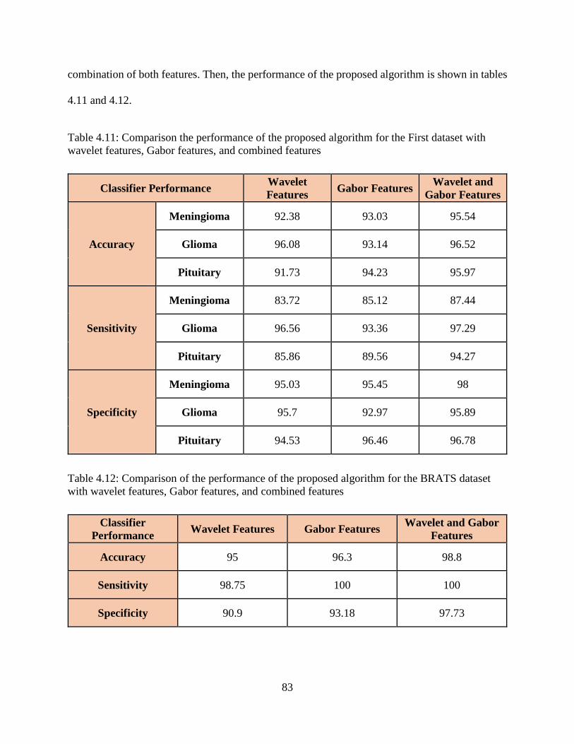
83
combination of both features. Then, the performance of the proposed algorithm is shown in tables
4.11 and 4.12.
Table 4.11: Comparison the performance of the proposed algorithm for the First dataset with
wavelet features, Gabor features, and combined features
Classifier Performance Wavelet
Features Gabor Features
Wavelet and
Gabor Features
Accuracy
Meningioma 92.38 93.03 95.54
Glioma 96.08 93.14 96.52
Pituitary 91.73 94.23 95.97
Sensitivity
Meningioma 83.72 85.12 87.44
Glioma 96.56 93.36 97.29
Pituitary 85.86 89.56 94.27
Specificity
Meningioma 95.03 95.45 98
Glioma 95.7 92.97 95.89
Pituitary 94.53 96.46 96.78
Table 4.12: Comparison of the performance of the proposed algorithm for the BRATS dataset
with wavelet features, Gabor features, and combined features
Classifier
Performance Wavelet Features Gabor Features
Wavelet and Gabor
Features
Accuracy 95 96.3 98.8
Sensitivity 98.75 100 100
Specificity 90.9 93.18 97.73

84
Wavelet features are generated using three levels of the 2-D DWT with the ‘symlet4’ filter,
while the Gabor features are generated using the 2-D Gabor filter with three wavelengths (2, 4,
and 8) and five orientations (0°,45°, 90°, 135°, and 180°). For each type of feature, the ten
statistical quantities (mean, variance, skewness, kurtosis, contrast, correlation, energy,
homogeneity, maximum probability, and entropy) are calculated for each image resulted from the
transformation. As stated in chapter three, combining both Wavelet Transform and Gabor filter
improve the performance of the classification since it utilized from all the directional information
of the MRI image. As shown in tables 4.11 and 4.12, the combined features outperform the
Wavelet features and Gabor features separately in terms of the total accuracy, sensitivity, and
specificity of the algorithm.
4.4.6 The Effect of Sparsity Regularization and L2-weight Regularization Coefficients on
the Performance of the Algorithm
As stated in section 3.4.4, regularization constraints increase the performance of the
autoencoder network by controlling the firing of neurons in the hidden layer. This regularization
was introduced in the design of the autoencoder network using two regularization term, sparsity
regularization and L2-weight Regularization. For each term, there is a coefficient that controls the
functionality of its regularization inside the cost function, which is shown in equation 3.67. To
study the effect of each coefficient, the accuracy of the algorithm was determined for different
values of sparsity regularization and the L2-weight regularization coefficients. This is shown in
figures 4.7 and 4.8 respectively. In fig. 4.7, the accuracy of the algorithm was calculated for the
values of sparsity regularization coefficient ranging from 0 to 10 in step of 0.5. The range of
accuracy for the first dataset is between 91.4% for a coefficient of 3 and 94.0% for a coefficient of
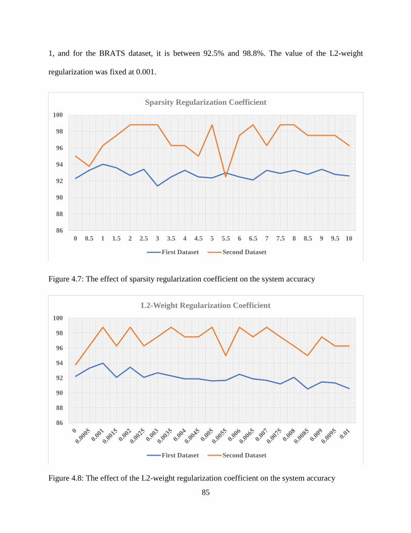
85
1, and for the BRATS dataset, it is between 92.5% and 98.8%. The value of the L2-weight
regularization was fixed at 0.001.
Figure 4.7: The effect of sparsity regularization coefficient on the system accuracy
Figure 4.8: The effect of the L2-weight regularization coefficient on the system accuracy
86
88
90
92
94
96
98
100
0 0.5 1 1.5 2 2.5 3 3.5 4 4.5 5 5.5 6 6.5 7 7.5 8 8.5 9 9.5 10
Sparsity Regularization Coefficient
First Dataset Second Dataset
86
88
90
92
94
96
98
100
L2-Weight Regularization Coefficient
First Dataset Second Dataset
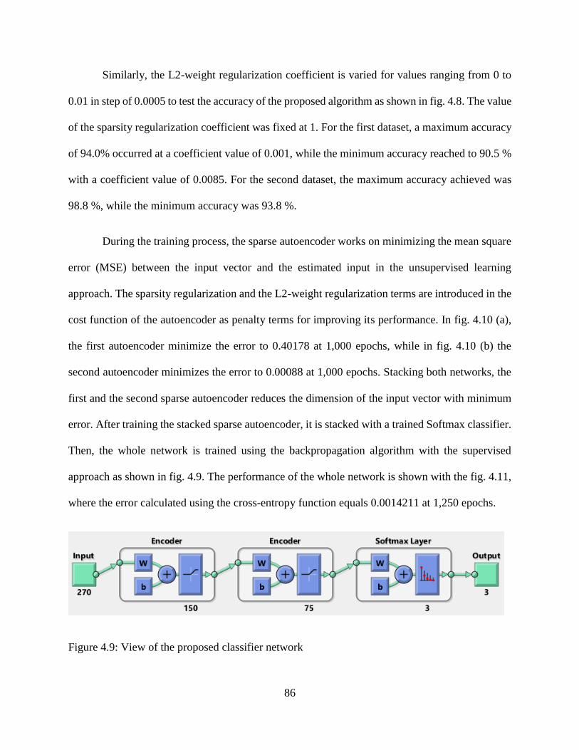
86
Similarly, the L2-weight regularization coefficient is varied for values ranging from 0 to
0.01 in step of 0.0005 to test the accuracy of the proposed algorithm as shown in fig. 4.8. The value
of the sparsity regularization coefficient was fixed at 1. For the first dataset, a maximum accuracy
of 94.0% occurred at a coefficient value of 0.001, while the minimum accuracy reached to 90.5 %
with a coefficient value of 0.0085. For the second dataset, the maximum accuracy achieved was
98.8 %, while the minimum accuracy was 93.8 %.
During the training process, the sparse autoencoder works on minimizing the mean square
error (MSE) between the input vector and the estimated input in the unsupervised learning
approach. The sparsity regularization and the L2-weight regularization terms are introduced in the
cost function of the autoencoder as penalty terms for improving its performance. In fig. 4.10 (a),
the first autoencoder minimize the error to 0.40178 at 1,000 epochs, while in fig. 4.10 (b) the
second autoencoder minimizes the error to 0.00088 at 1,000 epochs. Stacking both networks, the
first and the second sparse autoencoder reduces the dimension of the input vector with minimum
error. After training the stacked sparse autoencoder, it is stacked with a trained Softmax classifier.
Then, the whole network is trained using the backpropagation algorithm with the supervised
approach as shown in fig. 4.9. The performance of the whole network is shown with the fig. 4.11,
where the error calculated using the cross-entropy function equals 0.0014211 at 1,250 epochs.
Figure 4.9: View of the proposed classifier network
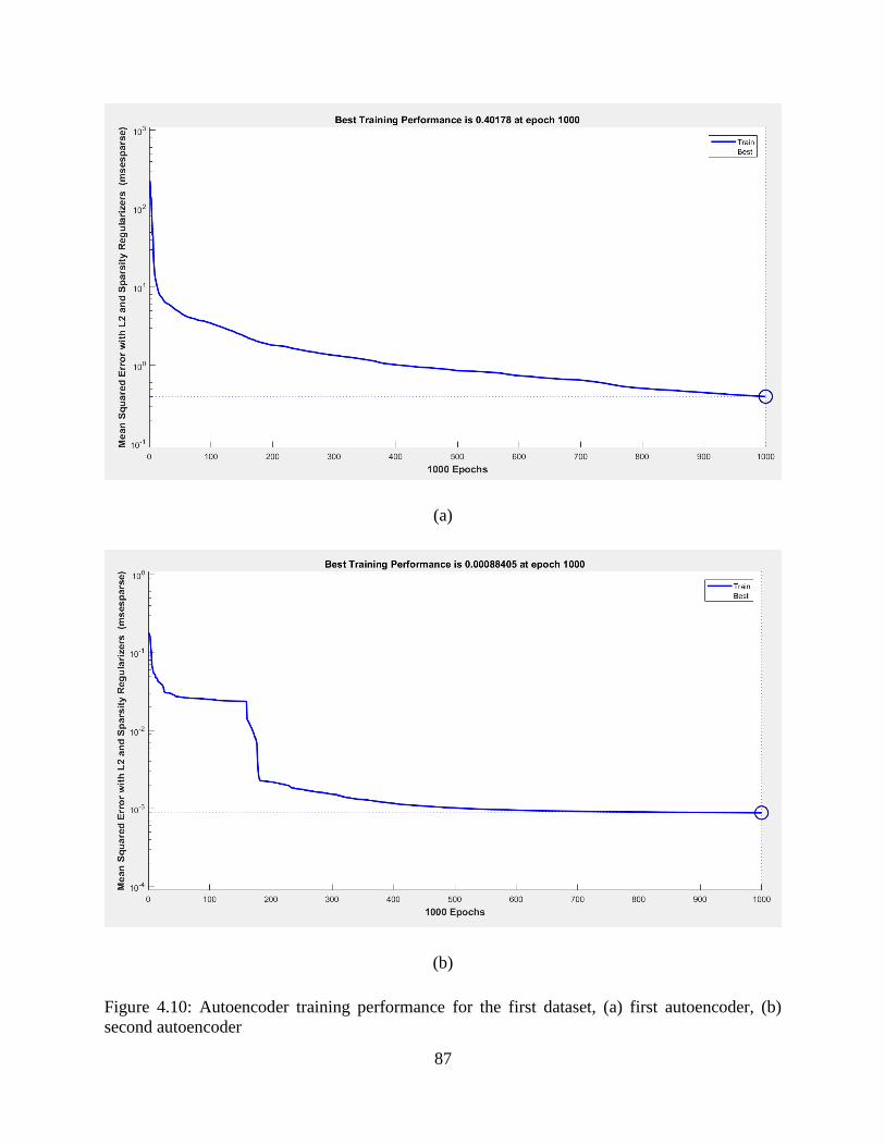
87
(a)
(b)
Figure 4.10: Autoencoder training performance for the first dataset, (a) first autoencoder, (b)
second autoencoder
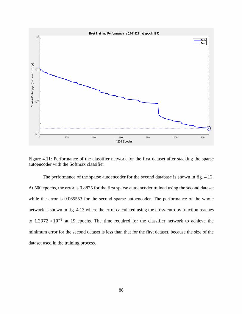
88
Figure 4.11: Performance of the classifier network for the first dataset after stacking the sparse
autoencoder with the Softmax classifier
The performance of the sparse autoencoder for the second database is shown in fig. 4.12.
At 500 epochs, the error is 0.8875 for the first sparse autoencoder trained using the second dataset
while the error is 0.065553 for the second sparse autoencoder. The performance of the whole
network is shown in fig. 4.13 where the error calculated using the cross-entropy function reaches
to 1.2972 ∗ 10−8 at 19 epochs. The time required for the classifier network to achieve the
minimum error for the second dataset is less than that for the first dataset, because the size of the
dataset used in the training process.
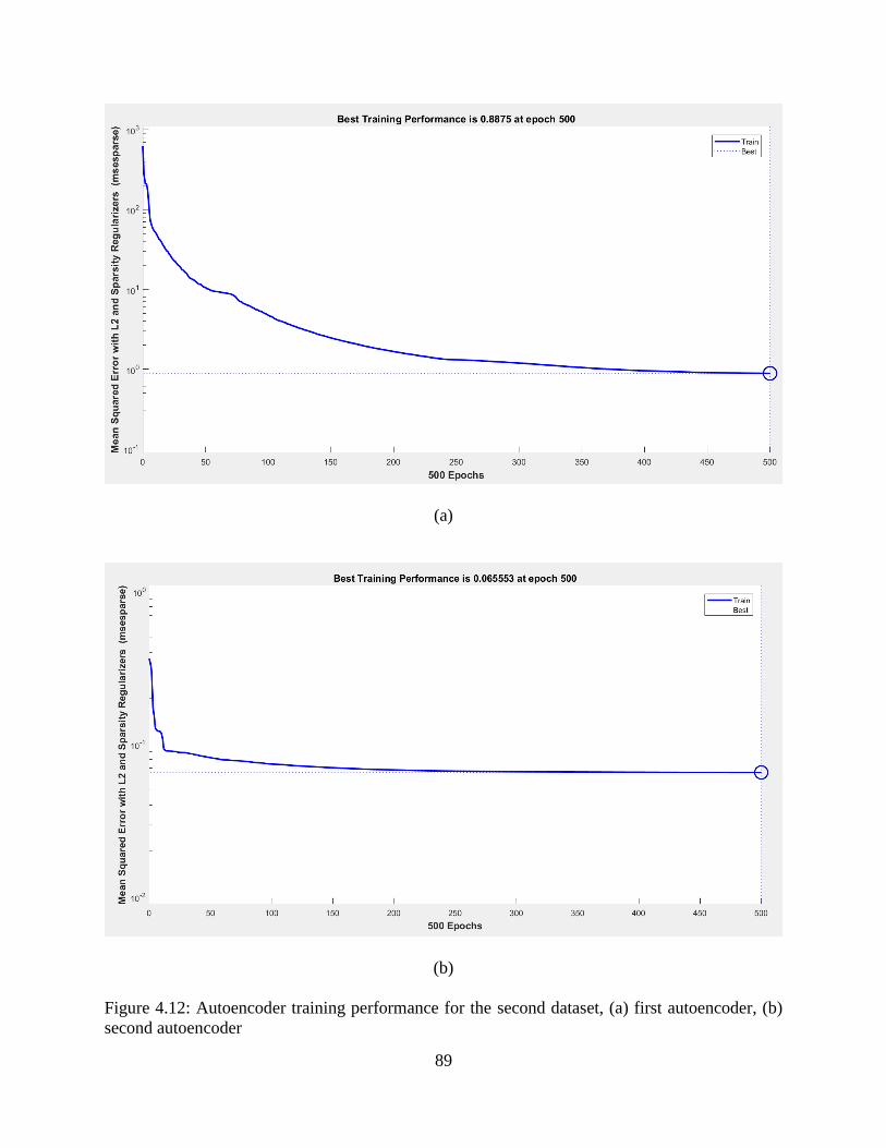
89
(a)
(b)
Figure 4.12: Autoencoder training performance for the second dataset, (a) first autoencoder, (b)
second autoencoder
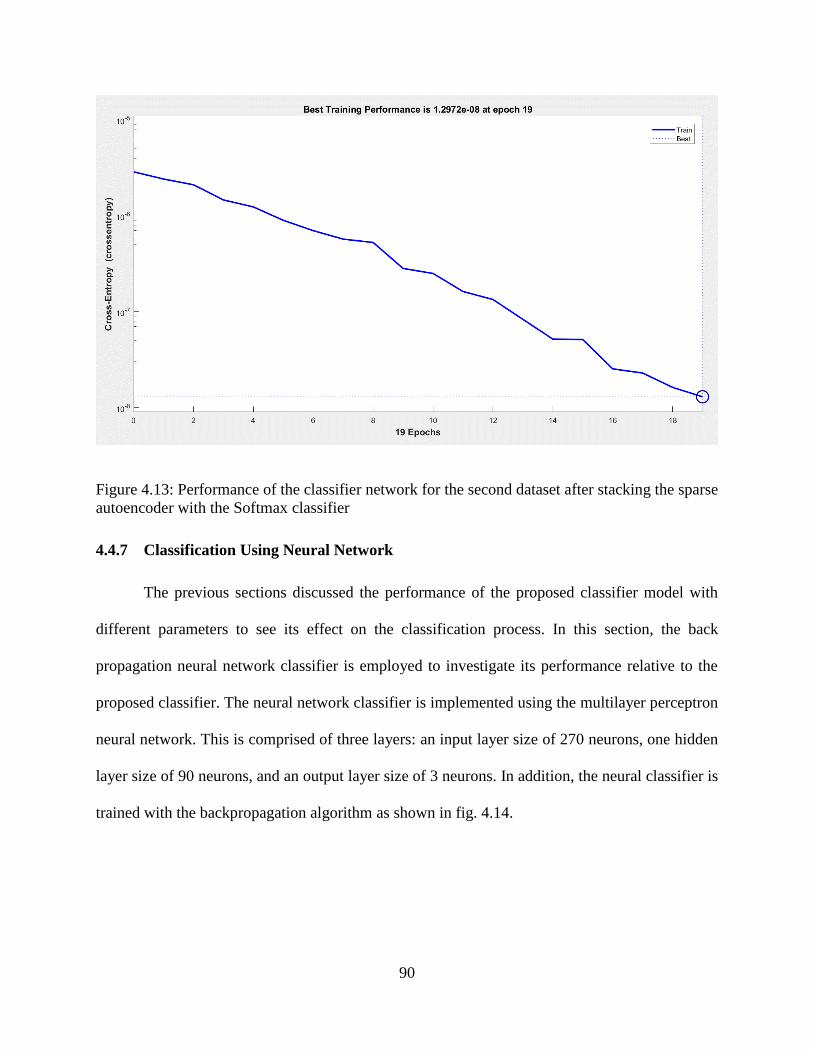
90
Figure 4.13: Performance of the classifier network for the second dataset after stacking the sparse
autoencoder with the Softmax classifier
4.4.7 Classification Using Neural Network
The previous sections discussed the performance of the proposed classifier model with
different parameters to see its effect on the classification process. In this section, the back
propagation neural network classifier is employed to investigate its performance relative to the
proposed classifier. The neural network classifier is implemented using the multilayer perceptron
neural network. This is comprised of three layers: an input layer size of 270 neurons, one hidden
layer size of 90 neurons, and an output layer size of 3 neurons. In addition, the neural classifier is
trained with the backpropagation algorithm as shown in fig. 4.14.
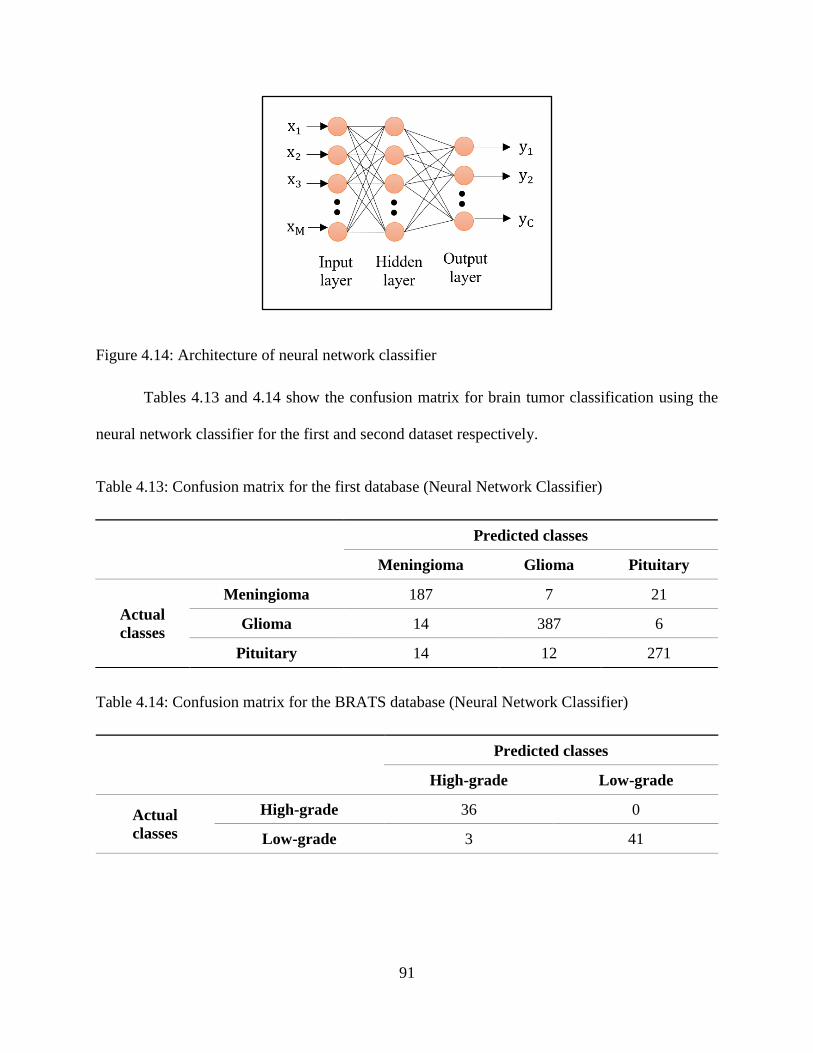
91
Figure 4.14: Architecture of neural network classifier
Tables 4.13 and 4.14 show the confusion matrix for brain tumor classification using the
neural network classifier for the first and second dataset respectively.
Table 4.13: Confusion matrix for the first database (Neural Network Classifier)
Table 4.14: Confusion matrix for the BRATS database (Neural Network Classifier)
Predicted classes
High-grade Low-grade
Actual
classes
High-grade 36 0
Low-grade 3 41
Predicted classes
Meningioma Glioma Pituitary
Actual
classes
Meningioma 187 7 21
Glioma 14 387 6
Pituitary 14 12 271
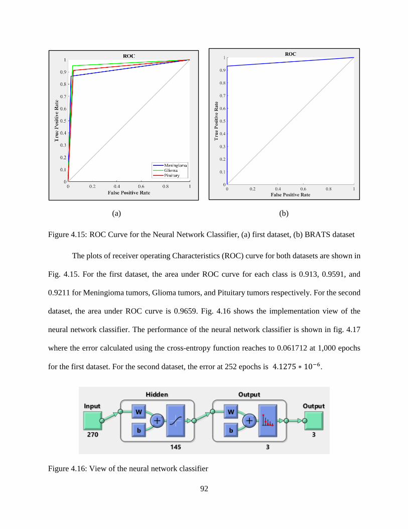
92
(a) (b)
Figure 4.15: ROC Curve for the Neural Network Classifier, (a) first dataset, (b) BRATS dataset
The plots of receiver operating Characteristics (ROC) curve for both datasets are shown in
Fig. 4.15. For the first dataset, the area under ROC curve for each class is 0.913, 0.9591, and
0.9211 for Meningioma tumors, Glioma tumors, and Pituitary tumors respectively. For the second
dataset, the area under ROC curve is 0.9659. Fig. 4.16 shows the implementation view of the
neural network classifier. The performance of the neural network classifier is shown in fig. 4.17
where the error calculated using the cross-entropy function reaches to 0.061712 at 1,000 epochs
for the first dataset. For the second dataset, the error at 252 epochs is 4.1275 ∗ 10−6.
Figure 4.16: View of the neural network classifier
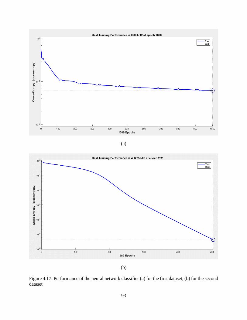
93
(a)
(b)
Figure 4.17: Performance of the neural network classifier (a) for the first dataset, (b) for the second
dataset

94
Table 4.15: Comparison of the performance of the proposed algorithm with neural network
classifier for the first dataset
Classifier Performance Wavelet
Features
Gabor
Features
Wavelet and
Gabor
Features
The
Proposed
Algorithm
Accuracy
Meningioma 92.38 93.03 95.54
Glioma 96.08 93.14 96.52
Pituitary 91.73 94.23 95.97
Sensitivity
Meningioma 83.72 85.12 87.44
Glioma 96.56 93.36 97.29
Pituitary 85.86 89.56 94.27
Specificity
Meningioma 95.03 95.45 98
Glioma 95.7 92.97 95.89
Pituitary 94.53 96.46 96.78
Neural
Network
Classifier
Accuracy
Meningioma 90.1 91.62 93.91
Glioma 94.89 91.73 95.75
Pituitary 90.21 92.27 94.23
Sensitivity
Meningioma 82.33 83.72 86.97
Glioma 94.1 91.65 95.1
Pituitary 82.5 85.52 91.24
Specificity
Meningioma 92.47 94.03 96
Glioma 95.51 91.8 96.29
Pituitary 93.89 95.5 95.66
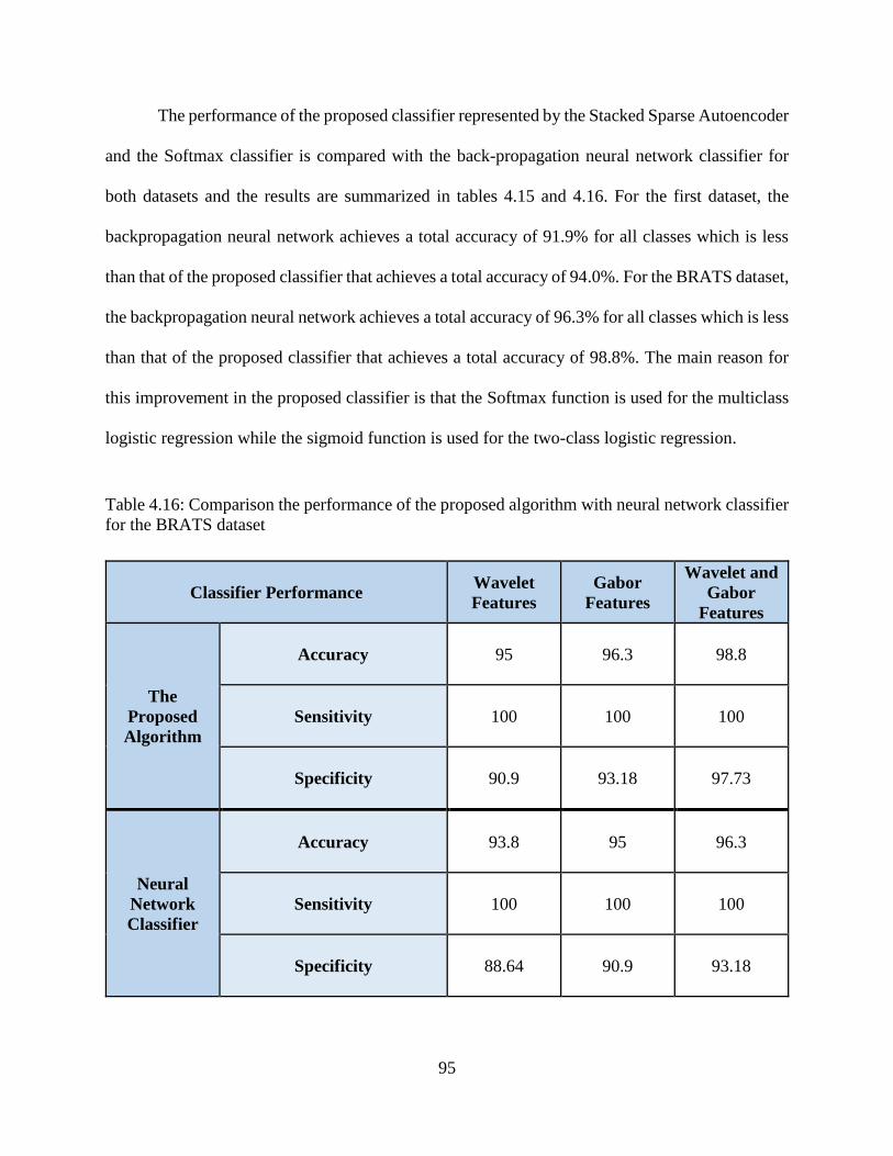
95
The performance of the proposed classifier represented by the Stacked Sparse Autoencoder
and the Softmax classifier is compared with the back-propagation neural network classifier for
both datasets and the results are summarized in tables 4.15 and 4.16. For the first dataset, the
backpropagation neural network achieves a total accuracy of 91.9% for all classes which is less
than that of the proposed classifier that achieves a total accuracy of 94.0%. For the BRATS dataset,
the backpropagation neural network achieves a total accuracy of 96.3% for all classes which is less
than that of the proposed classifier that achieves a total accuracy of 98.8%. The main reason for
this improvement in the proposed classifier is that the Softmax function is used for the multiclass
logistic regression while the sigmoid function is used for the two-class logistic regression.
Table 4.16: Comparison the performance of the proposed algorithm with neural network classifier
for the BRATS dataset
Classifier Performance Wavelet
Features
Gabor
Features
Wavelet and
Gabor
Features
The
Proposed
Algorithm
Accuracy 95 96.3 98.8
Sensitivity 100 100 100
Specificity 90.9 93.18 97.73
Neural
Network
Classifier
Accuracy 93.8 95 96.3
Sensitivity 100 100 100
Specificity 88.64 90.9 93.18
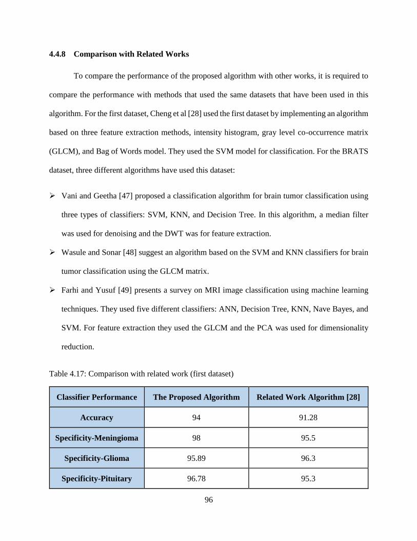
96
4.4.8 Comparison with Related Works
To compare the performance of the proposed algorithm with other works, it is required to
compare the performance with methods that used the same datasets that have been used in this
algorithm. For the first dataset, Cheng et al [28] used the first dataset by implementing an algorithm
based on three feature extraction methods, intensity histogram, gray level co-occurrence matrix
(GLCM), and Bag of Words model. They used the SVM model for classification. For the BRATS
dataset, three different algorithms have used this dataset:
➢ Vani and Geetha [47] proposed a classification algorithm for brain tumor classification using
three types of classifiers: SVM, KNN, and Decision Tree. In this algorithm, a median filter
was used for denoising and the DWT was for feature extraction.
➢ Wasule and Sonar [48] suggest an algorithm based on the SVM and KNN classifiers for brain
tumor classification using the GLCM matrix.
➢ Farhi and Yusuf [49] presents a survey on MRI image classification using machine learning
techniques. They used five different classifiers: ANN, Decision Tree, KNN, Nave Bayes, and
SVM. For feature extraction they used the GLCM and the PCA was used for dimensionality
reduction.
Table 4.17: Comparison with related work (first dataset)
Classifier Performance The Proposed Algorithm Related Work Algorithm [28]
Accuracy 94 91.28
Specificity-Meningioma 98 95.5
Specificity-Glioma 95.89 96.3
Specificity-Pituitary 96.78 95.3
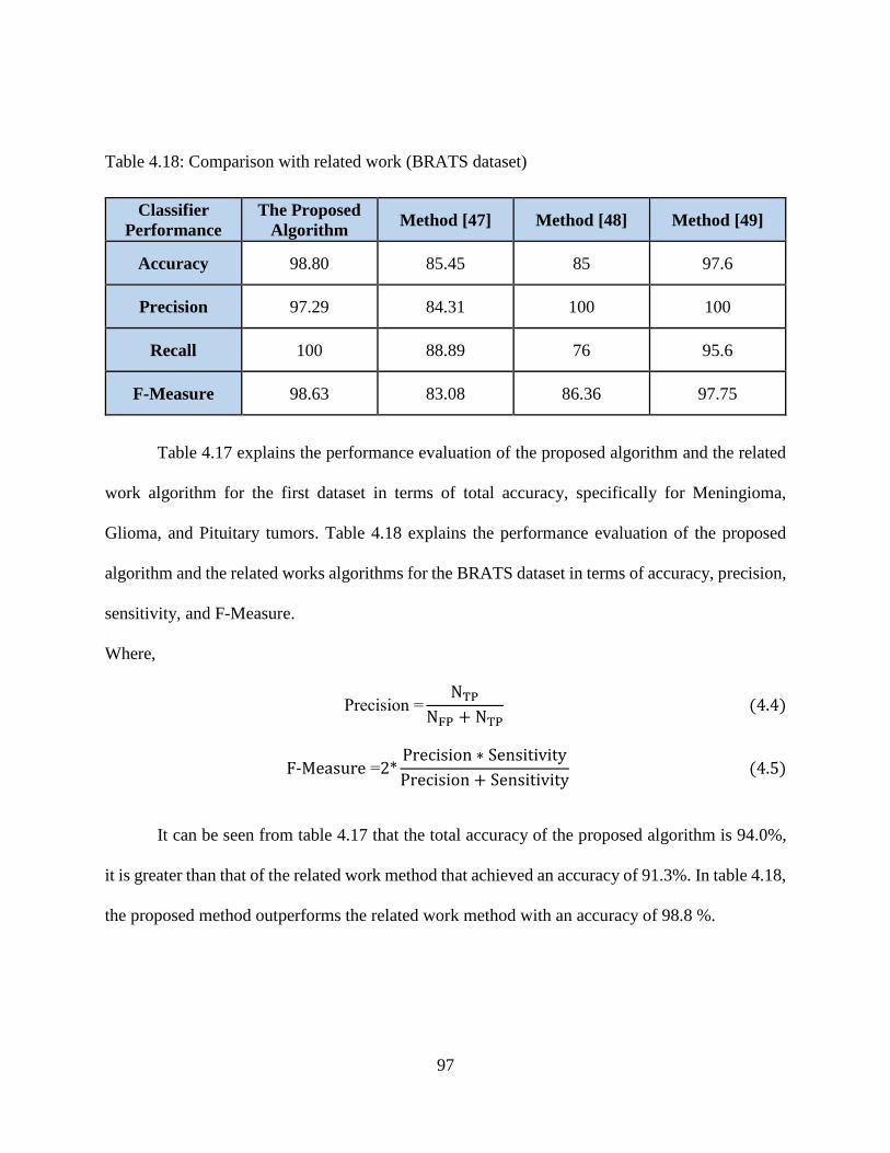
97
Table 4.18: Comparison with related work (BRATS dataset)
Classifier
Performance
The Proposed
Algorithm Method [47] Method [48] Method [49]
Accuracy 98.80 85.45 85 97.6
Precision 97.29 84.31 100 100
Recall 100 88.89 76 95.6
F-Measure 98.63 83.08 86.36 97.75
Table 4.17 explains the performance evaluation of the proposed algorithm and the related
work algorithm for the first dataset in terms of total accuracy, specifically for Meningioma,
Glioma, and Pituitary tumors. Table 4.18 explains the performance evaluation of the proposed
algorithm and the related works algorithms for the BRATS dataset in terms of accuracy, precision,
sensitivity, and F-Measure.
Where,
Precision =NTP
NFP + NTP (4.4)
F-Measure =2*Precision ∗ Sensitivity
Precision + Sensitivity (4.5)
It can be seen from table 4.17 that the total accuracy of the proposed algorithm is 94.0%,
it is greater than that of the related work method that achieved an accuracy of 91.3%. In table 4.18,
the proposed method outperforms the related work method with an accuracy of 98.8 %.

98
4.5 Implementation and Time Processing
Algorithms and techniques developed in chapter three are utilized and organized to be
implemented in a computer program written in MATLAB R2017a student license (9.2.0.538062)
and it is developed on a computer with a 2.6 GHz core i7 processor and a 16 Gigabyte RAM. As
discussed previously, the proposed algorithm is implemented in two phases; training phase and
testing phase. Table 4.19 summarizes the processing time for each method used in this algorithm.
The time measured for training is determined for all the slices used for training, while in the testing
phase the time is calculated for each slice to show how much time is taken to process each image
or ROI separately. The time measured for each slice is the time required for processing the
maximum tumor segment in the testing part of the database that has a size of 228 x 346. It is clear
from this table that this algorithm can recognize the type of tumor within 1.5 seconds.
Table 4.19: Processing time for training and testing phase
Phase Process Time in second
Training Classification 161
Testing
Wavelet Features/slice 0.125
Gabor Features/slice 1.1719
Total Features/slice 1.2968
Classification/slice 1.02e-04
4.6 Discussion of Results
To sum up, the proposed algorithm was applied to classify three types of tumors:
Meningioma, Glioma (high-grade and low-grade), and Pituitary, and used two datasets. For the

99
first dataset, 864 out of 919 MRI slices were correctly classified as its actual classes. The second
dataset classified 79 out of 80 MRI slices correctly. The combination of the Wavelet features and
the Gabor features improved the accuracy by 3.9% compared with the wavelet features only, and
it improved by 3.8% compared with the Gabor features only. Extracted features using the Gabor
filter are better than using the Gabor energy alone. The proposed classifier performance is sensitive
to any change in the sparsity regularization and the L2-weight regularization coefficients, but it
still achieves a high accuracy.
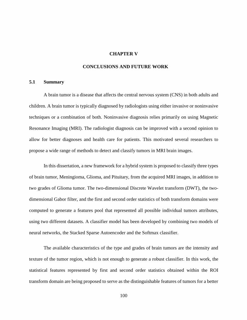
100
CHAPTER V
5.CONCLUSIONS AND FUTURE WORK
5.1 Summary
A brain tumor is a disease that affects the central nervous system (CNS) in both adults and
children. A brain tumor is typically diagnosed by radiologists using either invasive or noninvasive
techniques or a combination of both. Noninvasive diagnosis relies primarily on using Magnetic
Resonance Imaging (MRI). The radiologist diagnosis can be improved with a second opinion to
allow for better diagnoses and health care for patients. This motivated several researchers to
propose a wide range of methods to detect and classify tumors in MRI brain images.
In this dissertation, a new framework for a hybrid system is proposed to classify three types
of brain tumor, Meningioma, Glioma, and Pituitary, from the acquired MRI images, in addition to
two grades of Glioma tumor. The two-dimensional Discrete Wavelet transform (DWT), the two-
dimensional Gabor filter, and the first and second order statistics of both transform domains were
computed to generate a features pool that represented all possible individual tumors attributes,
using two different datasets. A classifier model has been developed by combining two models of
neural networks, the Stacked Sparse Autoencoder and the Softmax classifier.
The available characteristics of the type and grades of brain tumors are the intensity and
texture of the tumor region, which is not enough to generate a robust classifier. In this work, the
statistical features represented by first and second order statistics obtained within the ROI
transform domain are being proposed to serve as the distinguishable features of tumors for a better
101
discriminatory process against the types/grades of brain tumors. The Gabor filter has the
significant property of orientation selectivity, while the 2-D DWT results in three directional
information, Therefore, the 2-D Gabor filter and the 2-D DWT are combined as directional
transformation feature set and their combination improves the classification accuracy when
compared to using each method separately. The classifier model comprised of two types of neural
network, the stacked sparse autoencoder, and the Softmax classifier. The main goal of the
autoencoder is to convert a high dimensional input vector to a low dimension vector obtained from
the hidden layer by minimizing the error between the input and the output.
In addition, the hybrid system composed of the Wavelet-Gabor statistical features improves
the accuracy of the classification as compared to using each feature set separately. This allowed
for the development of richer tumor type specific features and a better discriminative process
among the tumors. Despite its sensitivity to any change in the sparsity regularization and L2-
weight regularization coefficients, the Stacked Sparse Autoencoder still achieves an excellent
accuracy and exhibits a high-performance classification when combined with the Softmax
classifier.
Two datasets were used to train and test the proposed algorithm. The first one consists of
3,064 slices of T1-weighted MRI images with three kinds of tumors: Meningioma, Glioma, and
Pituitary. The second dataset has 200 MRI images with high and low grades of Glioma tumors.
The proposed system performance was measured using accuracy, sensitivity, and specificity.
Results show the effectiveness of the classification implemented by the stacked Softmax classifier
with the stacked sparse autoencoder. There was an accuracy of 94.0% for the first dataset and
98.8% for the BRATS dataset.

102
5.2 Contribution
The main contribution of this dissertation is the development of the integrated Stacked
Sparse Autoencoder and the Softmax classifier as a complete classification system suitable for the
delicacy of type and grade of MRI brain tumor identification. Unlike the backpropagation neural
network classifier, the proposed classification system trains each layer separately, controls the
firing of each neuron in the hidden layer, and reduces the overfitting. This is achievable because
the Softmax function (within the Softmax classifier) is designed for the multiclass logistic
regression compared to the sigmoid function (used by the backpropagation neural network
classifier) that is restricted to two-class logistic regression. This proposed system can be a useful
tool for the radiologist as a second opinion for tumor diagnoses
5.3 Future Works
Improvements can be always made by adding features that stem from the specific dataset
or the MRI equipment. For example, separating patients’ images between male and female
patients, or separating images between children and adult patients. In addition, it will be
informative to develop a large dataset at national level and compare the results for subsets.
103
BIBLIOGRAPHY
[1] M. S. H. Al-Tamimi and G. Sulong, “TUMOR BRAIN DETECTION THROUGH MR
IMAGES: A REVIEW OF LITERATURE.,” J. Theor. Appl. Inf. Technol., vol. 62, no. 2,
2014.
[2] American Cancer Society, “What Are the Key Statistics About Brain and Spinal Cord
Tumors?,” 2018. .
[3] E.-S. A. El-Dahshan, H. M. Mohsen, K. Revett, and A.-B. M. Salem, “Computer-aided
diagnosis of human brain tumor through MRI: A survey and a new algorithm,” Expert Syst.
Appl., vol. 41, no. 11, pp. 5526–5545, 2014.
[4] M. K. Abd-Ellah, A. I. Awad, A. A. M. Khalaf, and H. F. A. Hamed, “Design and
implementation of a computer-aided diagnosis system for brain tumor classification,” in
Microelectronics (ICM), 2016 28th International Conference on, 2016, pp. 73–76.
[5] H. Selvaraj, S. T. Selvi, D. Selvathi, and L. Gewali, “Brain MRI slices classification using
least squares support vector machine,” Int. J. Intell. Comput. Med. Sci. Image Process., vol.
1, no. 1, pp. 21–33, 2007.
[6] D. M. Joshi, N. K. Rana, and V. M. Misra, “Classification of brain cancer using artificial
neural network,” in Electronic Computer Technology (ICECT), 2010 International
Conference on, 2010, pp. 112–116.
[7] N. Zulpe and V. Pawar, “GLCM textural features for brain tumor classification,” IJCSI Int.
104
J. Comput. Sci. Issues, vol. 9, no. 3, pp. 354–359, 2012.
[8] P. John and others, “Brain tumor classification using wavelet and texture based neural
network,” Int. J. Sci. Eng. Res., vol. 3, no. 10, pp. 1–7, 2012.
[9] S. D. S. Al-Shaikhli, M. Y. Yang, and B. Rosenhahn, “Brain tumor classification using
sparse coding and dictionary learning,” in Image Processing (ICIP), 2014 IEEE
International Conference on, 2014, pp. 2774–2778.
[10] V. Anitha and S. Murugavalli, “Brain tumour classification using two-tier classifier with
adaptive segmentation technique,” IET Comput. Vis., vol. 10, no. 1, pp. 9–17, 2016.
[11] D. Glass-Macenka, L. Hays, A. Varner, E. Weiss, and P. Y. Wen, “Tumor Types:
Understanding Brain Tumors,” in Frankly Speaking About Cancer series, Cancer Support
Community, 2013.
[12] D. N. Louis et al., “The 2007 WHO classification of tumours of the central nervous system,”
Acta Neuropathol., vol. 114, no. 2, pp. 97–109, 2007.
[13] B. H. Menze et al., “The multimodal brain tumor image segmentation benchmark
(BRATS),” IEEE Trans. Med. Imaging, vol. 34, no. 10, pp. 1993–2024, 2015.
[14] S. Bauer, R. Wiest, … L. N.-P. in medicine and, and undefined 2013, “A survey of MRI-
based medical image analysis for brain tumor studies,” Iopscience.Iop.Org, pp. 1–44.
[15] R. Support and A. P. F. Gaillard, “No Title.” [Online]. Available:
https://radiopaedia.org/articles/meningioma.
[16] D. Y. Weerakkody and A. P. F. Gaillard, “No Title.” [Online]. Available:

105
https://radiopaedia.org/articles/pituitary-tumours.
[17] N. Nabizadeh, “Automated brain lesion detection and segmentation using magnetic
resonance images,” University of Miami, 2015.
[18] D. C. Preston, “Magnetic Resonance Imaging (MRI) of the Brain and Spine: Basics,” 2006.
[19] S. Theodoridis and K. Koutroumbas, pattern recognition. Academic Press, 2009.
[20] G. Dougherty, Digital image processing for medical applications. Cambridge University
Press, 2009.
[21] S. A. Ali, S. Vathsal, and K. L. Kishore, “An efficient denoising technique for CT images
using window-based multi-wavelet transformation and thresholding,” Eur. J. Sci. Res., vol.
48, no. 2, p. 315, 2010.
[22] S. G. Chang, B. Yu, and M. Vetterli, “Adaptive wavelet thresholding for image denoising
and compression,” IEEE Trans. image Process., vol. 9, no. 9, pp. 1532–1546, 2000.
[23] S. Arivazhagan et al., “Performance Analysis of Wavelet filters for image denoising,” Adv.
Comput. Sci. Technol., vol. 1, no. 1, pp. 1–10, 2007.
[24] S. Shen, W. Sandham, M. Granat, and A. Sterr, “MRI fuzzy segmentation of brain tissue
using neighborhood attraction with neural-network optimization,” IEEE Trans. Inf.
Technol. Biomed., vol. 9, no. 3, pp. 459–467, 2005.
[25] Y. Kabir, M. Dojat, B. Scherrer, F. Forbes, and C. Garbay, “Multimodal MRI segmentation
of ischemic stroke lesions,” in Engineering in Medicine and Biology Society, 2007. EMBS
2007. 29th Annual International Conference of the IEEE, 2007, pp. 1595–1598.
106
[26] N. Gordillo, E. Montseny, and P. Sobrevilla, “State of the art survey on MRI brain tumor
segmentation,” Magn. Reson. Imaging, vol. 31, no. 8, pp. 1426–1438, 2013.
[27] F. Y. Shih, Image processing and pattern recognition: fundamentals and techniques. John
Wiley & Sons, 2010.
[28] J. Cheng et al., “Enhanced performance of brain tumor classification via tumor region
augmentation and partition,” PLoS One, vol. 10, no. 10, p. e0140381, 2015.
[29] P. Dvorak, W. Kropatsch, and K. Bartusek, “Automatic detection of brain tumors in MR
images,” 2013 36th Int. Conf. Telecommun. Signal Process., pp. 577–580, 2013.
[30] N. Sumitra and R. K. Saxena, “Brain tumor classification using back propagation neural
network,” Int. J. Image, Graph. Signal Process., vol. 5, no. 2, p. 45, 2013.
[31] K. Rashmi, S. Ramadoss, and L. K. Sandhya, “Brain Tumor Detection Using SVM
Classifier,” pp. 318–323, 2017.
[32] G. L. Qurat-Ul-Ain, S. B. Kazmi, M. A. Jaffar, and A. M. Mirza, “Classification and
segmentation of brain tumor using texture analysis,” Recent Adv. Artif. Intell. Knowl. Eng.
data bases, pp. 147–155, 2010.
[33] K. D. Kharat, P. P. Kulkarni, and M. B. Nagori, “Brain tumor classification using neural
network based methods,” Int. J. Comput. Sci. Informatics, vol. 1, no. 4, pp. 2231–5292,
2012.
[34] P. M. S. Kumar and S. Chatteijee, “Computer aided diagnostic for cancer detection using
MRI images of brain (Brain tumor detection and classification system),” in India
Conference (INDICON), 2016 IEEE Annual, 2016, pp. 1–6.
107
[35] U. Javed, M. M. Riaz, A. Ghafoor, and T. A. Cheema, “MRI brain classification using
texture features, fuzzy weighting and support vector machine,” Prog. Electromagn. Res. B,
vol. 53, pp. 73–88, 2013.
[36] V. Kumar, J. Sachdeva, I. Gupta, N. Khandelwal, and C. K. Ahuja, “Classification of brain
tumors using PCA-ANN,” in Information and Communication Technologies (WICT), 2011
World Congress on, 2011, pp. 1079–1083.
[37] J. Sachdeva, V. Kumar, I. Gupta, N. Khandelwal, and C. K. Ahuja, “Multiclass brain tumor
classification using GA-SVM,” in Developments in E-systems Engineering (DeSE), 2011,
2011, pp. 182–187.
[38] J. Sachdeva, V. Kumar, I. Gupta, N. Khandelwal, and others, “A dual neural network
ensemble approach for multiclass brain tumor classification,” Int. j. numer. method. biomed.
eng., vol. 28, no. 11, pp. 1107–1120, 2012.
[39] E. I. Zacharaki et al., “Classification of brain tumor type and grade using MRI texture and
shape in a machine learning scheme,” Magn. Reson. Med., vol. 62, no. 6, pp. 1609–1618,
2009.
[40] A. Vidyarthi and N. Mittal, “Performance analysis of Gabor-Wavelet based features in
classification of high grade malignant brain tumors,” in Systems Conference (NSC), 2015
39th National, 2015, pp. 1–6.
[41] Y. Zhang and L. Wu, “An MR brain images classifier via principal component analysis and
kernel support vector machine,” Prog. Electromagn. Res., vol. 130, pp. 369–388, 2012.
[42] Y. Liu, M. Muftah, T. Das, L. Bai, K. Robson, and D. Auer, “Classification of MR tumor
108
images based on Gabor wavelet analysis,” J. Med. Biol. Eng., vol. 32, no. 1, pp. 22–28,
2012.
[43] E. I. Zacharaki et al., “MRI-based classification of brain tumor type and grade using SVM-
RFE,” in Biomedical Imaging: From Nano to Macro, 2009. ISBI’09. IEEE International
Symposium on, 2009, pp. 1035–1038.
[44] K. M. Priya, S. Kavitha, and B. Bharathi, “Brain tumor types and grades classification based
on statistical feature set using support vector machine,” in Intelligent Systems and Control
(ISCO), 2016 10th International Conference on, 2016, pp. 1–8.
[45] K. A. Johnson and J. A. Becker, “The whole brain atlas.” the authors, 1999.
[46] K. Clark et al., “The Cancer Imaging Archive (TCIA): maintaining and operating a public
information repository,” J. Digit. Imaging, vol. 26, no. 6, pp. 1045–1057, 2013.
[47] V. Vani, “Automatic Tumor Classification of Brain MRI Images,” vol. 7, no. 10, pp. 144–
151, 2016.
[48] V. Wasule, “Classification of Brain MRI Using SVM and KNN Classifier,” pp. 218–223,
2017.
[49] L. Farhi and A. Yusuf, “Comparison of Brain Tumor MRI Classification Methods Using
Probabilistic Features,” Biomed. Eng. (NY)., no. BioMed, pp. 55–62, 2017.
[50] J. Cheng, “brain tumor dataset,” 2017.
[51] M. Machakowsalya, J. Nivethitha, and A. N. Kumar, “Brain Tumor Classification and
Segmentation in MRI Images using PNN,” 2017.

109
[52] G. Singh and M. A. Ansari, “Efficient detection of brain tumor from MRIs using K-means
segmentation and normalized histogram,” India Int. Conf. Inf. Process. IICIP 2016 - Proc.,
vol. 1, no. 2, 2017.
[53] C. C. Benson, V. L. Lajish, and K. Rajamani, “Robust Classification of MR Brain Images
Based on Fractal Dimension Analysis,” pp. 1135–1140, 2017.
[54] B. Sudha, P. Gopikannan, A. Shenbagaraj, and C. Balasubramanian, “Classification of
Brain Tumor Grades using Neural Network,” in Proceedings of the World Congress on
Engineering 2014, 2014, vol. 1.
[55] S. E. Grigorescu, N. Petkov, and P. Kruizinga, “Comparison of texture features based on
Gabor filters,” IEEE Trans. Image Process., vol. 11, no. 10, pp. 1160–1167, 2002.
[56] N. Aggarwal and R. K. Agrawal, “First and second order statistics features for classification
of magnetic resonance brain images,” J. Signal Inf. Process., vol. 3, no. 2, p. 146, 2012.
[57] R. Sonavane, “Classification Of MRI Brain Tumor and Mammogram Images Using
Learning Vector Quantization Neural Network,” pp. 301–307, 2017.
[58] K. D. Kharat, V. J. Pawar, and S. R. Pardeshi, “Feature extraction and selection from MRI
images for the brain tumor classification,” 2016 Int. Conf. Commun. Electron. Syst., pp. 1–
5, 2016.
[59] A. Kharrat, K. Gasmi, and M. B. E. N. Messaoud, “A Hybrid Approach for Automatic
Classification of Brain MRI Using Genetic Algorithm and Support Vector Machine,”
Leonardo J. Sci., no. 17, pp. 71–82, 2010.
[60] A. Kharrat, M. B. Halima, and M. Ben Ayed, “MRI brain tumor classification using Support
110
Vector Machines and meta-heuristic method,” Int. Conf. Intell. Syst. Des. Appl. ISDA, vol.
2016–June, no. January 2016, 2016.
[61] S. Lahmiri and M. Boukadoum, “Classification of brain MRI using the LH and HL wavelet
transform sub-bands,” Proc. - IEEE Int. Symp. Circuits Syst., pp. 1025–1028, 2011.
[62] C. S. Engineering, J. Singh, and C. Engineering, “Classification of Brain MRI in Wavelet
Domain,” no. Ll, pp. 879–885, 2011.
[63] S. Shingade and P. Jain, “Identification of Brain Tumor using Gabor Wavelets Techniques,”
vol. 4, no. 2, 2017.
[64] M. F. Othman and M. A. M. Basri, “Probabilistic neural network for brain tumor
classification,” in Intelligent Systems, Modelling and Simulation (ISMS), 2011 Second
International Conference on, 2011, pp. 136–138.
[65] S. S. Haykin, S. S. Haykin, S. S. Haykin, and S. S. Haykin, Neural networks and learning
machines, vol. 3. Pearson Upper Saddle River, NJ, USA:, 2009.
[66] G. P. Zhang, “Neural networks for classification: a survey,” IEEE Trans. Syst. Man, Cybern.
Part C (Applications Rev., vol. 30, no. 4, pp. 451–462, 2000.
[67] A. T. C. Goh, “Probabilistic neural network for evaluating seismic liquefaction potential,”
Can. Geotech. J., vol. 39, no. 1, pp. 219–232, 2002.
[68] T. Kohonen, “Exploration of very large databases by self-organizing maps,” Int. Conf.
Neural Networks, p. PL1-PL6, 1997.
[69] H. Byun and S.-W. Lee, “Applications of support vector machines for pattern recognition:
111
A survey,” Pattern Recognit. with Support vector Mach., pp. 571–591, 2002.
[70] A. Halder, “Rough K-means and Support Vector Machine based Brain Tumor Detection,”
pp. 116–120, 2017.
[71] R. Ahmmed, A. Sen Swakshar, F. Hossain, and A. Rafiq, “Classification of Tumors and It
Stages in Brain MRI Using Support Vector Machine and Artificial Neural Network,” pp.
229–234, 2017.
[72] S. Ghanavati, J. Li, T. Liu, P. S. Babyn, W. Doda, and G. Lampropoulos, “Automatic brain
tumor detection in magnetic resonance images,” in Biomedical Imaging (ISBI), 2012 9th
IEEE International Symposium on, 2012, pp. 574–577.
[73] S. Lahmiri, M. Boukadoum, S. Lahmiri, and M. Boukadoum, “Hybrid Discrete Wavelet
Transform and Gabor Filter Banks Processing for Features Extraction from Biomedical
Images,” J. Med. Eng., vol. 2013, pp. 1–13, 2013.
[74] C. Liu and H. Wechsler, “Gabor feature based classification using the enhanced fisher linear
discriminant model for face recognition.,” IEEE Trans. Image Process., vol. 11, no. 4, pp.
467–476, 2002.
[75] P. S. Addison, The illustrated wavelet transform handbook: introductory theory and
applications in science, engineering, medicine and finance. CRC press, 2017.
[76] G. Zauner, M. Reiter, D. Salaberger, and J. Kastner, “Denoising of computed tomography
images using multiresolution based methods,” Proc. ECNDT, Berlin Sept, 2006.
[77] R. C. Gonzalez and R. E. Woods, “Digital image processing,” Up. Saddle River, NJ, 2014.
112
[78] S. K. Shukla and A. K. Tiwari, Efficient algorithms for discrete wavelet transform: with
applications to denoising and fuzzy inference systems. Springer Science & Business Media,
2013.
[79] A. Maksumov, R. Vidu, A. Palazoglu, and P. Stroeve, “Enhanced feature analysis using
wavelets for scanning probe microscopy images of surfaces,” J. Colloid Interface Sci., vol.
272, no. 2, pp. 365–377, 2004.
[80] P. D. Shukla, “Complex wavelet transforms and their applications,” University of
Strathclyde, 2003.
[81] H. N. Al-Taai, “Computationally efficient wavelet based algorithms for optical flow
estimation,” Ph. D. Thesis, Univ. of Technology, Electrical and electronic engineering, Dep,
2005.
[82] D. Gabor, “Theory of communication. Part 1: The analysis of information,” J. Inst. Electr.
Eng. III Radio Commun. Eng., vol. 93, no. 26, pp. 429–441, 1946.
[83] V. S. N. Prasad and J. Domke, “Gabor filter visualization,” J. Atmos. Sci, vol. 13, p. 2005,
2005.
[84] R. Roslan and N. Jamil, “Texture feature extraction using 2-D Gabor Filters,” in Computer
Applications and Industrial Electronics (ISCAIE), 2012 IEEE Symposium on, 2012, pp.
173–178.
[85] T. S. Lee, “Image representation using 2D Gabor wavelets,” IEEE Trans. Pattern Anal.
Mach. Intell., vol. 18, no. 10, pp. 959–971, 1996.
[86] J. Yang, L. Liu, T. Jiang, and Y. Fan, “A modified Gabor filter design method for fingerprint
113
image enhancement,” Pattern Recognit. Lett., vol. 24, no. 12, pp. 1805–1817, 2003.
[87] B. Karlik and A. V. Olgac, “Performance analysis of various activation functions in
generalized MLP architectures of neural networks,” Int. J. Artif. Intell. Expert Syst., vol. 1,
no. 4, pp. 111–122, 2011.
[88] C. M. Bishop, Pattern recognition and machine learning. springer, 2006.
[89] A. Ng, “Sparse autoencoder,” CS294A Lect. notes, vol. 72, no. 2011, pp. 1–19, 2011.
[90] D. P. Mandic, “A generalized normalized gradient descent algorithm,” IEEE Signal
Process. Lett., vol. 11, no. 2, pp. 115–118, 2004.
[91] Y. Guo, Y. Gao, and D. Shen, “Deformable MR prostate segmentation via deep feature
learning and sparse patch matching,” IEEE Trans. Med. Imaging, vol. 35, no. 4, pp. 1077–
1089, 2016.
[92] I. Goodfellow, Y. Bengio, and A. Courville, Deep learning. MIT press, 2016.
[93] M. H. Beale, M. T. Hagan, and H. B. Demuth, “Neural Network ToolboxTM User’s Guide,”
Mathworks Inc, 1992.
[94] J. M. Joyce, “Kullback-leibler divergence,” in International Encyclopedia of Statistical
Science, Springer, 2011, pp. 720–722.
[95] J. Xu et al., “Stacked sparse autoencoder (SSAE) for nuclei detection on breast cancer
histopathology images,” IEEE Trans. Med. Imaging, vol. 35, no. 1, pp. 119–130, 2016.
[96] M. Kubat, An Introduction to Machine Learning. Springer, 2015.
114
[97] T. Sing, O. Sander, N. Beerenwinkel, and T. Lengauer, “ROCR: visualizing classifier
performance in R,” Bioinformatics, vol. 21, no. 20, pp. 3940–3941, 2005.
[98] T. A. Lasko, J. G. Bhagwat, K. H. Zou, and L. Ohno-Machado, “The use of receiver
operating characteristic curves in biomedical informatics,” J. Biomed. Inform., vol. 38, no.
5, pp. 404–415, 2005.
[99] K. Markham, “Simple guide to confusion matrix terminology,” Data Sch. [online], 2014.