Embed Size (px)
Citation preview
JOSAI MATHEMATICAL MONOGRAPHS Vol. 2 (2000) pp. 91 - 104
Hybrid Method for Solving Polynomial Equations
LillOng ZHI YOShiO NOTAKE HiroShi KAI Matu-TarOW
Ehime Univ.
K.1. SHIRAISHI t
Takuma National College of Technology
NODA +
Abstract
We discuss how to decompose the zero set of a multivariate polynomial system with inexact coefficients to a sequence of zero sets of reduced triangular sets in a numerically
stable way.
1 Introductlon
Finding the solutions to a system of non-1inear polynomial equations over a given field
is a classical and fundamental problem in the computational literature. Many problems
in robotics, computer vision, computational geometry, signal processing involve solving
polynomial systems of equations. A number of symbolic, numeric and hybrid approaches
have been proposed. Newton's algorithms and homotopy methods are two main numeric
approaches for solving zero-dimensional polynomial systems. Newton's method works well
only if we are given good initial guesses to the solutions and it is difficult for most prac-
tical problems. Since 1970's, the rapid advances in techniques for homotopy method have
brought a great leap in the feasibility of solving numerical polynomial systems globally [8]
[1l]. However, it still suffers some problems such as path=crossing[12].
Most papers on symbolic or hybrid methods(combination of symbolic and numeric ap-
proaches) for polynomial solving concentrate on Gr6bner basis and resultant method. It is
well known that Gr6bner basis method can not be applied safely with floating point arith-
metic and requires to increase the precision of computation dramatically compared with
input and output precision. Algorithm based on resultant method provides one of the most
'{lzhi ,notake,kai ,noda } @hpc.cs.ehime-u.ac.jp
91
92 Procedings of NLA99 (2000)
efficient solution method for small and mediumsize zero-dimensional polynomial systems
[3][18]. Different kinds of resultant matrices are used for constructing monomial bases,
multiplication maps and, ultimately, reduce solving a polynomial system to an eigenvalue
problem. On the other hand, as directly applying resultant for polynomial solving, Wu
Wen-tstin developed the theory of subresultant for reducing a polynomial system to a fam-
ily of triangular sets. The subresultant polynomial remainder sequence is well known as
the best nonmodular algorithm for computing GCD and resultant of sparse multivariate
polynomials [1][2] [4] [5] . However, its application in polynomial solving is still relatively
unexplored. In [13] , Noda and Sasaki have used subresultant theory for computing ap-
proximate GCD of multivariate polynomials and then, applied it to solve ill-condition
polynomial systems. But their purpose is to divide out the approximate GCD and transfer
the system to well-condition problem.
In this paper, we combine Wu's symbolic elimination theory with Noda and Sasaki's
approximate GCD computation to solve systems of polynomial equations with numeric
coefiicients. Our paper is organized as follows. In section 2 we describe Wu's method,
followed in section 3 by generalizing it to polynomials with numerical coefficients. Section
4 compares the current approach with the Gr6bner basis method.
2 Wu9S Elimination Theory
2 . I P reliminaries
R Let K be a field of characteristic O and let xl' ' ' " x~ be a set of indeterminates with
the order x ~ x ~: xn K[xl""'x~] is the ring of polynomials in these variables.
R Let c be the greatest subscript such that xc actually occurs in f. We define:
1. cls(f) = the class of f = c.
2. Iv(f) = the leading variable of f = xc'
3. cdeg(f) = the class degree of f = degx.f.
4. ini(f) = the initial of f with respect to lv(f) = coeff(f, xc' cdeg(f). Note that ini(f)
, xc-l] ' is a polynomial in K[xl' ' ' '
R A polynomial g is said to be reduced with respect to f if degx.(9) < cdeg(f).
e Let PS = {pl'p2, . ' ' ,ps} be a polynomial set in K[xl' ' ' " x~], PS is called a triangular
set if either s = I and pl ~ O, or s > I and cls(pl) < cls(p2) < ・ ・ ・ < cls(ps)' If s > 1
and pj is reduced with respect to pi for each pair j > i, then PS is called an ascending
set. An ascending set is said to be contradictory if $ = I and pl is a non-zero constant.
Josai Mathematical Monographs Vol. 2 (2000) 93
o For a nonempty polynomial set PS ~ K[xl, ' ' ' , x~], the greatest class c, if it exists,
for which the number of corresponding polynomial is > I , is called the dominant class
of PS, the least degree of polynomials having class c is called the dominant degree of
PS. In case, no such c > O exists then dominant class will be defined to be O, while
dominant degree will be left undefined.
c For polynomial sets PS and polynomial G. Zero(PS) denotes the zero set of PS,
Zero(PS/G) for Zero(PS) - Zero(G).
2.2 SubreSultant Cham
Let f and g be two multrvanate polynonuals m K[x , Xn] Suppose lv(f) Iv(g) = x
and m = cdeg(f) ~ cdeg(g) = : n
f = fmxm+...+fo, fm~0. (1) g = gnxn+...+go, 9n~0. (2)
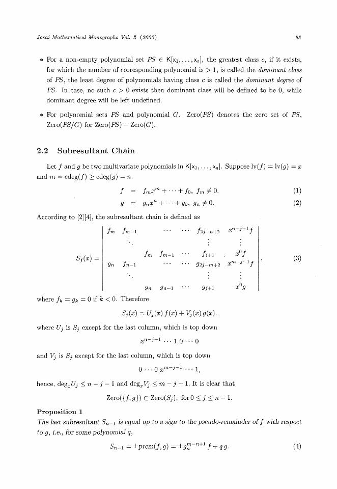
According to [2] [4] , the subresultant chain is defined as
fm fm-1 ' ' ' f2j-n+2 xn-j-I f
Sj(x) = gn fn I fm fm-1 ' ' ' fj+1 xof (3) f ' m-j-1 ' ' ' 92j-m+2 x
9n 9n I ' 9j+1 xog where fk = gk = O if k < O. Therefore
Sj(x) = Uj(x) f(x) + Vj(x) g(x).
where Uj is Sj except for the last column, which is top down
xn-j-1 . " 10-'O and Vj is Sj except for the last column, which is top down
O"'Oxm 3 1 ... 1,
hence, degxUj ~ n - j - I and degxVj < m - j - 1. It is clear that
Zero({f,g}) C Zero(Sj)' forO ~ j ~ n - 1.
Proposition 1
The last subresultant Sn-1 is equal up to a sign to the pseudo-remainder of f with respect
to g, i.e., for some polynomial q,
f + qg. Snl n
94 Procedings of NLA99 (2000)
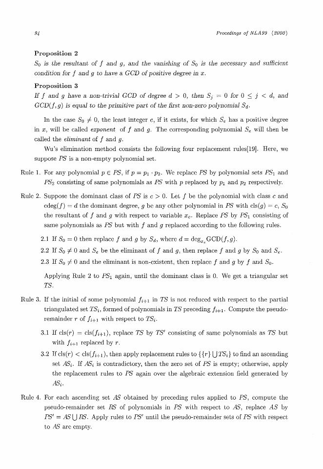
Proposition 2
So is the resultant of f and g, and the vanishing of So is the necessary and sui~icient
condition for f and g to have a GCD ofpositive degree in x.
Proposition 3
If f and g have a non-trivial GCD of degree d > o, then Sj = O for O ~ j < d, and
GCD(f, g) is equal to the primitive part of the frst non-zero polynomial Sd .
In the case So ~ O, the least integer e, if it exists, for which S* has a positive degree
in x, will be called exponent of f and g. The corresponding polynomial S* will then be
called the eliminant of f and g.
Wu's elimination method consists the following four replacement rules[19]. Here, we
suppose PS is a nonempty polynomial set.
Rule I . For any polynomial p e pS, if p = pl ' p2 . We replace PS by polynomial sets PSI and
PS2 consisting of same polynomials as PS with p replaced by pl and p2 respectively.
Rule 2. Suppose the dominant class of PS is c > O. Let f be the polynomial with class c and
cdeg(f) = d the dominant degree, g be any other polynomial in PS with cls(g) = c, So
the resultant of f and g with respect to variable x*. Replace PS by PSI consisting of
same polynomials as PS but with f and g replaced according to the following rules.
2.1 If So = O then replace f and g by Sd, where d = deg*.GCD(f, g).
2.2 If So ~ O and S* be the eliminant of f and g, then replace f and g by So and S* .
2.3 If So ~ O and the eliminant is non-existent, then replace f and g by f and So .
Applying Rule 2 to PSI again, until the dominant class is O. We get a triangular set
TS.
Rule 3 If the mitlal of some polynomlal fi+1 m TS is not reduced with respect to the partial
triangulated set TSi, formed of polynomials in TS preceding fi+1 ' Compute the pseudo
remainder r of fi+1 with respect to TSi.
3.1 If cls(r) = cls(fi+1), replace TS by TS/ consisting of same polynomials as TS but
with fi+1 replaced by r.
3.2 If cls(r) < cls(fi+1), then apply replacement rules to {{r} U TSi} to flnd an ascending
set ASi . If ASi is contradictory, then the zero set of PS is empty; otherwise, apply
the replacement rules to PS again over the algebraic extension field generated by
ASi .
Rule 4. For each ascending set AS obtained by preceding rules applied to PS, compute the
pseudo-remainder set RS of polynomials in PS with respect to AS, replace AS by
ps! = AS U RSL Apply rules to PS/ until the pseudo-remainder sets of PS with respect
to AS are empty.
Joson Mathematzcal Monographs Vol. 2 (2000) 95
Applying replacement rule 1-4 whenever possible. Ultimately, we have the following
theorem.
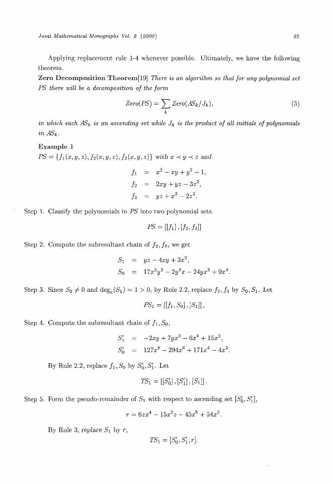
Zero Decomposition Theorem[19] There is an algorithm so that for any polynomial set
PS there will be a decomposition of the form
Zero(PS) = ~ Zero(ASk/Jh) (5)
in which each ASk is an ascending set while Jk is the product of all initials of polynomials
in ASk .
Example 1 PS = {fl(x, y, z), f2(x, y, z), f3(x, y, z)} with x ~: y ~ z and
fl = x2-xy+y2-1, f2 = 2xy + yz - 3z2
f3 = yz+x2 -2z2.
Step I . Classify the polynomials in PS into two polynomial sets.
PS = [[fl] ' [f2, f3]]
Step 2. Compute the subresultant chain of f2 , f3 , we get
S1 = yz - 4xy + 3x2
So = 17x2y2 - 2y3x - 24yx3 + 9x4.
Step 3. Since So ~ O and degz(Sl) = I > o, by Rule 2.2, replace f2, f3 by So, Sl ' Let
PSI = [[fl' So] , [Si]] ,
Step 4. Compute the subresultant chain of fl ' So ,
S{ = -2xy + 7yx3 - 6x4 + 15x2
S/o = 127x8 - 294x6 + 17lx4 - 4x2.
By Rule 2.2, replace fl' So by S6, Si・ Let
TSI = [[S6] , [S{] , [Sl]] '
Step 5. Form the pseudo-remainder of Sl with respect to ascending set [S6, Si],
r = 6zx4 - 15x2z - 45x5 + 54x
By Rule 3, replace S1 by r,
TSI = [So, S1' r]
96 Procedings of NLA99 (2000)
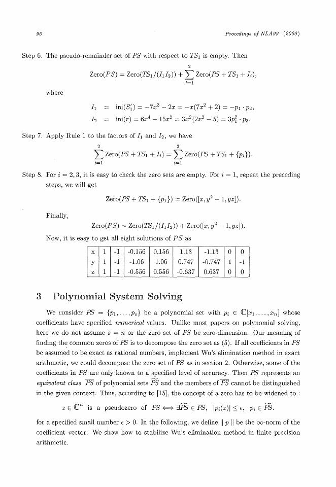
Step 6.
Step 7.
Step 8.
The pseudo-remainder set of PS with respect to TSI rs empty. Then
Zero(PS) Zero(TS /(1112)) + i Zero(PS + TS + I~)'
i=1
where
I1 = ini(S{) = -7x3 - 2x = -x(7x2 + 2) = -pl 'p2,
12 = ini(r) = 6x4 - 15x2 = 3x2(2x2 - 5) = 3p~ ・p3'
Apply Rule I to the factors of 11 and 12 , we have
~ Zero(PS + TS + I ) ~ Zero(PS + TS + {p })
For i = 2, 3, it is easy to check the zero sets are empty. For i = 1, repeat the preceding
steps, we will get
Zero(PS + TS + {p }) Zero([x,y2 - 1,yz]).
Finally,
Zero(PS) Zero(TS /(1112)) + Zero([x, y2 - 1, yz]).
Now, it is easy to get all eight solutions of PS as
x y z
1 1 1
-1
-1
-1
-0.156
- I .06
-0.556
0.156
1.06
0.556
1.13
0.747
-0.637
-1.13
-0.747
0.637
O
o
o
o
3 POlynOmial SyStem SolVing
We consider PS = {pl' ' ' "ps} be a polynomial set with pi e C[xl' ' ' " xn] whose
coefficients have specifled numerical values. Unlike most papers on polynomial solving,
here we do not assume s = n or the zero set of PS be zero-dimension. Our meaning of
flnding the common zeros of PS is to decompose the zero set as (5). If all coefficients in PS
be assumed to be exact as rational numbers, implement Wu's elimination method in exact
arithmetic, we could decompose the zero set of PS as in section 2. Otherwise, some of the
coefficients in PS are only known to a specified level of accuracy. Then PS represents an
equivalent class PS of polynomial sets PS and the members of PS cannot be distinguished
in the given context. Thus, according to [15] , the concept of a zero has to be= widened to :
z e Cn rs a pseudozero of PS <~> ~PS e PS Ip (z)1 < e, pi e PS.
for a specified small number c > O. In the following, we deflne jl p ll be the oo-norm of the
coefficient vector. We show how to stabilize Wu's elimination method in flnite precision
arithmetic.
Josai Mathematical Monograplts Vol. 2 (2000) 97
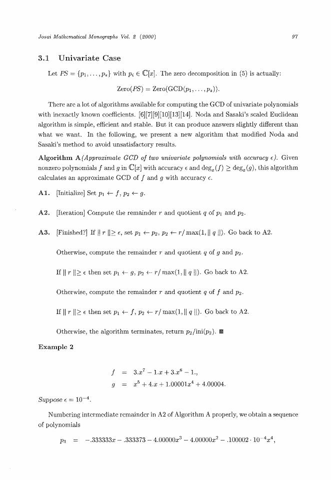
3.1 Univariate Case
Let PS = {pl' ' ' "p.} with pi ~ C[x]. The zero decomposition in (5) is actually:
Zero(PS) = Zero(GCD(pl' ' ' " p.)).
There are a lot of algorithms available for computing the GCD of univariate polynomials
with inexactly known coeflicients. [6] [7] [9] [10] [13] [14] . Noda and Sasaki's scaled Euclidean
algorithm is simple, efiicient and stable. But it can produce answers slightly different than
what we want. In the following, we present a new algorithm that modified Noda and
Sasaki's method to avoid unsatisfactory results.
Algorithm A(Approximate GCD of two univariate polynomials with accuracy e). Given
nonzero polynomials f and g in C[x] with accuracy 6 and deg. (f) ~ deg. (g), this algorithm
calculates an approximate GCD of f and g with accuracy c.
A1. [Initialize] Set pl ~~ f,p2 ~ 9.
A2. [Iteration] Compute the remainder r and quotient q of pl and p2 .
A3. [Finished?] If ll r llZ e, set pl ~ p2, p2 ~ r/max(1, 11 q II)・ Go back to A2.
Otherwise, compute the remainder r and quotient q of g and p2 .
If ll r llZ 6 then set pl ~~ g, p2 ~ r/max(1 11 q ll) Go back to A2
Otherwise, compute the remainder r and quotient q of f and p2 .
If ll r ll~ e then set pl ~~ f, p2 <- r/max(1, Il q ll)・ Go back to A2.
Otherwise, the algorithm terminates, return p2/ini(p2). I~
Example 2
f = 3.x7-1.x+3.x6 - 1.,
g = x5 + 4.x + 1.0000lx4 + 4 OO004
Suppose e = 10-4.
Numbering intermediate remainder in A2 of Algorithm A properly, we obtain a sequence
of polynomials
p3 = -.333333x - .333373 - 4.00000x3 - 4.00000x2 - .100002 ・ 10-4x4
98 Procedings of NLA99 (2000)
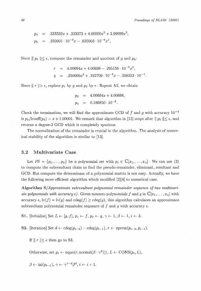
p4 :::
p5 :~
.333332x + .333373 + 4.00000x2 + 3.99999x3
250001 ・ 10~9x - .625003 ・ 10~9x2
Since li p5 ii~ e, compute the remainder and quotient of g and p4:
= 4.00694x + 4.00698 - .295158 ・ 10~5x2
q = 250000x + 192706 10 x 208353 ・ 10-1.
Since ll r ll> e, replace pl by g and p2 by r. Repeat A2 we obtam
p3 = 4.00694x + 4.00698,
p4 = 0.186850 ・ 10~8.
Check the termination, we will find the approximate GCD of f and g with accuracy 10-4
is p3/1coeff(p3) = x + 1.00001. We remark that algorithm in [13] stops after 11 p5 Il~ e, and
returns a degree-3 GCD which is completely spurious.
The normalization of the remainder is crucial in the algorithm. The analysis of numer-
ical stability of the algorithm is similar to [13] .
3.2 Multivariate Case
Let PS = {pl' ' ' "ps} be a polynomial set with pi e C[xl' ' ' " xn]' We can use (3)
to compute the subresultant chain to find the pseudo-remainder, eliminant, resultant and
GCD. But compute the determinant of a polynomial matrix is not easy. Actually, we have
the following more efficient algorithm which modifled [2] [4] to numerical case.
Algorithm S(Approximate subresultant polynomial remainder sequence of two multivari-
ate polynomials with accuracy e). Given nonzero polynomials f and g in C[xl' ' ' ' , xn] with
accuracy e, Iv(f) = Iv(g) and cdeg(f) ~ cdeg(g), this algorithm calculates an approximate
subresultant polynomial remainder sequence of f and g with accuracy e.
S1. [Initialize] Set L <~ [g, f], pl <~ f, p2 ~ 9, ~/ ~~ 1, p ~ I ~ ~~ 3
S2. [Iteration] Set d ~ cdeg(pi-2) - cdeg(p 1) r ~ nprem(p~ 2 Pe l)
If ll r ll~ ~ then go to S3.
Otherwise, set pi <- nquo(r) normal(p . 7d))), L ~ CONS(pi, L),
p ~ ini(pi-1), 7 ~ n/1-dpd z ~ ~ + 1
Josai Mathematical Monographs Vol. 2 (2000) 99
S3. [Finished?] If ll r jl< e or deg*(r) = O then set L ~ INV(L), return L.
Otherwise, go back to S2. IB
The function CONS(pi,L) appends pi to the list L and INV(L) reverses the list L.
Note that the division to get pi in S2 is exact if the coeflicients are exact rational nurnbers.
Otherwise, we impose the similar normalization of quotient as in the case of univariate poly-
nomials. If cls(g) = O then nquo(f, g) = f/9・ Otherwise, suppose the pseudo-remainder r
and quotient q of f and g with respect to x = Iv(g) be calculated by
ml(g) f - qg, d = deg (f) cdeg(g) + I > O (6)
If 11 r ll / Il ini(g)d ll~ e then
nquo(f, g) = nquo (q, ini(g)d) .
Otherwise, return f/ll 9 11 as the quotient. Since the class of divisor decreases, finally,
we can stop to get a polynomial divided by a number. Let q,d be the same in (6), the
normalizations of the pseudo-remainders and polynomials are
nprem(f,g) = r/max(lini(g)d ll,llqll),
normal(f) = flllfll-
See [13] for the analysis of numerical stability of the algorithm.
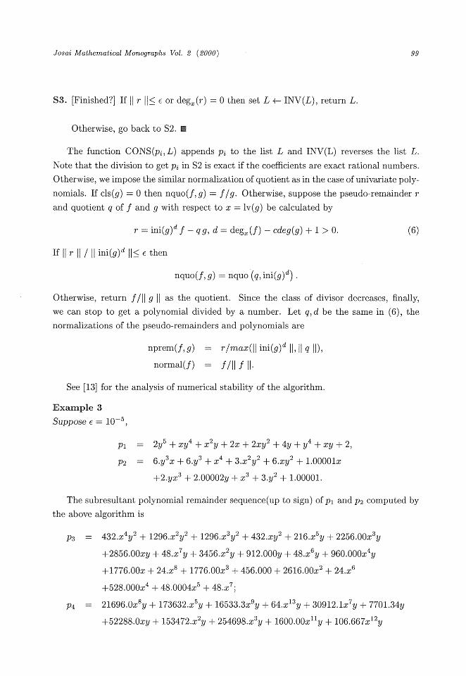
Example 3 Suppose e = 10-5
pl = 2y5 + xy4 + x2y + 2x + 2xy2 + 4y + y4 + xy + 2,
p2 = 6.y3x + 6.y3 + x4 + 3.x2y2 + 6.xy2 + 1.0000lx
+2.yx3 + 2.00002y + x3 + 3.y2 + 1.00001.
The subresultant polynomial remainder sequence(up to sign) of pl and p2 computed by
the above algorithm is
p3 = 432.x4y2 + 1296.x2y2 + 1296.x3y2 + 432.xy2 + 216.x5y + 2256.00x3y
+2856.00xy + 48.x7y + 3456.x2y + 912.000y + 48.x6y + 960.000x4y
+1776.00x + 24.x8 + 1776.00x3 + 456.000 + 2616.00x2 + 24.x6
+528.000x4 + 48.0004x5 + 48.x7.
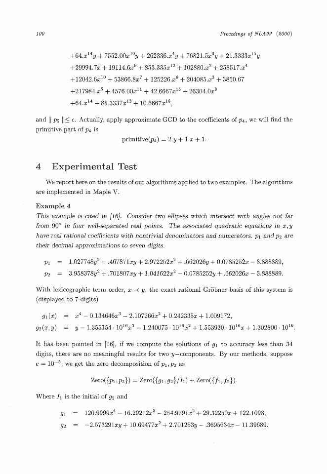
p4 = 21696.0x8y + 173632.x5y + 16533.3x9y + 64.xl3y + 30912.1x7y + 7701.34y
+52288.0xy + 153472.x2y + 254698.x3y + 1600.00xlly + 106.667xl2y
100 Procedings of NLA99 (2000)
+64 xl4y + 7552.00xroy + 262336.x4y + 76821.5x6y + 21.3333xl5y
+29994.7x + 19114.6x9 + 853.335xl2 + 102880.x2 + 258517.x4
+12042 6xlo ~ 53866 8x + 125226.x6 + 204085.x3 + 3850.67
+217984.x5 + 4576.00xll + 42 6667xl5 + 26304 Ox
+64.xl4 + 85.3337xl3 + 10.6667xl6
and ji p5 ii~ c. Actually, apply approximate GCD to the coeflicients of p4 , we will find the
primitive part of p4 is
primitive(p4) = 2.y + 1.x + 1.
4 EXperimental TeSt
We report here on the results of our algorithms applied to two examples. The algorithms
are implemented in Maple V.
Example 4 This example is cited in fl6J. Consider two ellipses which intersect with angles not far
from 90' in four well-separated real points. The associated quadratic equations in x,y
have real rational coei~icients with nontrivial denominators and numerators. pl and p2 are
their decimal approximations to seven digits.
pl = 1.027748y2 - .46787lxy + 2.972252x2 + .662026y + 0.0785252x - 3.888889,
p2 = 3.958378y2 + .701807xy + 1.041622x2 - 0.0785252y + .662026x - 3.888889.
With lexicographic term order, x ~ y, the exact rational Gr6bner basis of this system is
(displ'ayed to 7-digits)
91(x) = x4 - 0.134646x3 - 2.107266x2 + 0.242335x + 1.009172,
92(x,y) = y - 1.355154 ・ 1016x3 - 1.240075 ・ 1016x2 + 1.553930 ・ 1016x + 1.302800 ・ 1016
It has been pointed in [16], if we compute the solutions of gl to accuracy less than 34
digits, there are no meaningful results for two y-components. By our methods, suppose
e = 10-5 we get the zero decomposition of pl'p2 as
Zero({pl'p2}) = Zero({91 92}/1 ) + Zero({fl f2})
Where ll is the initial of g2 and
91 = 120.9999x4 - 16.29212x3 - 254.979lx2 + 29.32250x+ 122.l098,
92 = -2.57329lxy + 10.69477x2 + 2.701253y - .3695634x - 11.39689.
Josai Mathematical Monographs Vol. 2 (2000) 1 ol
Solve gl for Digits = 10(the number of digits carried in floats),
x = 1 204415, -.7603909, 1.049726, 1.049726.
Substitute the first two zeros to g2 , the initial 11 rs nonzero, and we get
y = -.7865145, 1.058881.
which are exact to six digits. Evaluate 11 at the last two zeros, we find it is less than 10-5.
Now, we consider another branch
fl = 1.000000x - 1.049727,
f2 = 2.254914y2 + .3749366y - 1.165602.
There are two sets of solutions
{x = 1.049727, y = -.8068975},
{x = 1.049727, y = .6406222}.
Substitute the solutions to pl 'p2, the error is less than 10-5.
For this example, using Maple's fsolve, it only gives one set of solutions corresponding
-.8068975}・ In order to find the other three roots, we have to give to {x = 1.049727, y =
appropriate range informations.
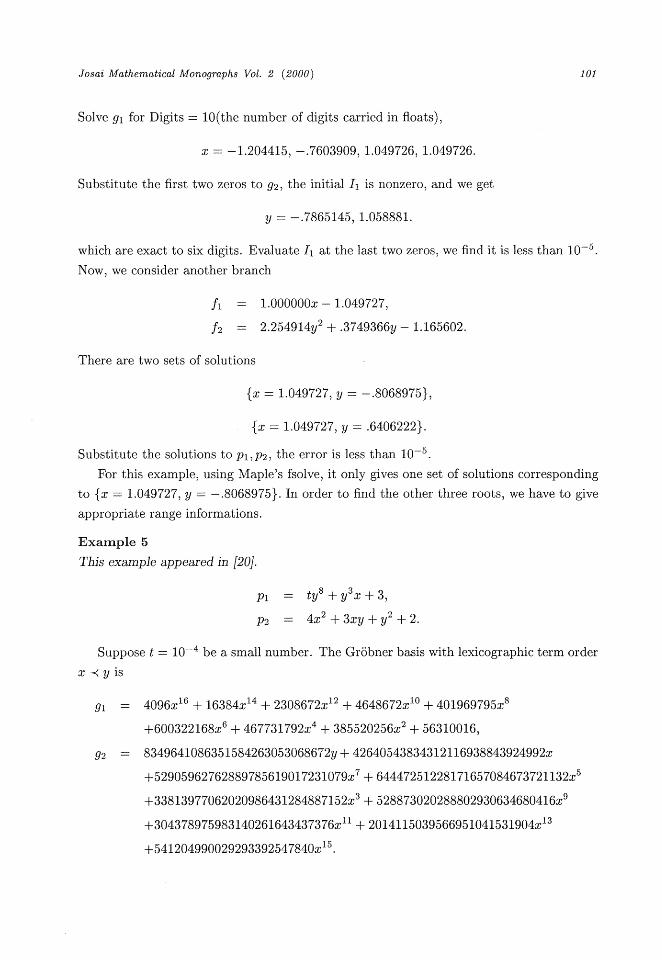
Example 5 This example appeared in f20J.
pl = ty8 + y3x+3,
p2 = 4x2+3xy+y2+2.
Suppose t = 10- be a small number The Grobner basrs wrth lexrcographic term order
x ~ y is
91 = 4096xl6 + 16384xl4 h 2308672xl2 + 4648672xlo + 401969795x8
+600322168x6 + 467731792x4 H~ 385520256x2 + 56310016,
92 = 8349641086351584263053068672y + 42640543834312116938843924992x
+52905962762889785619017231079x7 + 6444725 12281 71657084673721 132x5
+33813977062020986431284887152x3 + 528873020288802930634680416x9
+304378975983140261643437376xl I + 20141 15039566951041531904xl3
+541204990029293392547840xl5
1 02 Procedings of NLA99 (2000)
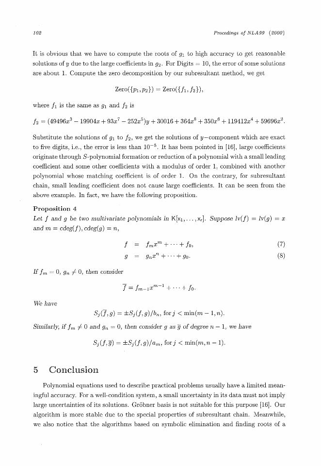
It is obvious that we have to compute the roots of gl to high accuracy to get reasonable
solutions of y due to the large coeflicients in g2. For Digits = 10, the error of some solutions
are about 1. Compute the zero decomposition by our subresultant method, we get
Zero({pl'p2}) = Zero({fl f2})
where fl is the same as gl and f2 is
f2 = (49496x 19904x + 93x 252x )y + 30016+364x + 350x + 119412x + 59696x
Substitute the solutions of gl to f2 , we get the solutions of y-component which are exact
to flve digits, i.e., the error is less than 10-5. It has been pointed in [16], Iarge coefiicients
originate through S-polynomial formation or reduction of a polynomial with a small leading
coeflicient and some other coefficients with a modulus of order 1, combined with another
polynomial whose matching coefncient is of order I . On the contrary, for subresultant
chain, small leading coeflicient does not cause large coeflicients. It can be seen from the
above example. In fact, we have the following proposition.
Proposition 4
Let f and g be two multivariate polynomials in K[xl' ' ' " Xr] Suppose lv(f) Iv(g) = x
and m = cdeg(f), cdeg(g) = n,
f = fmxm+...+fo, (7) g = gnxn+...+go (8)
If fm = O, gn ~ O then conslder
f = fmlxm I + + fo
We have
Sj(f, g) = ~Sj(f, g)/bn' for j < min(m - 1, n).
Similarly; if fm ~ O and gn = O, then consider g as ~ of degree n - I , we have
Sj(f,~) = ~Sj(f, g)lam' forj < min(m, n - 1).
5 ConcluSion Polynomial equations used to describe practical problems usually have a limited mean-
ingful accuracy. For a well-condition system, a small uncertainty in its data must not imply
large uncertainties of its solutions. Gr6bner basis is not suitable for this purpose [16]. Our
algorithm is more stable due to the special properties of subresultant chain. Meanwhile,
we also notice that the algorithms based on symbolic elimination and flnding roots of a
Josai Mathematical Monographs Vol. 2 (2000) 1 03
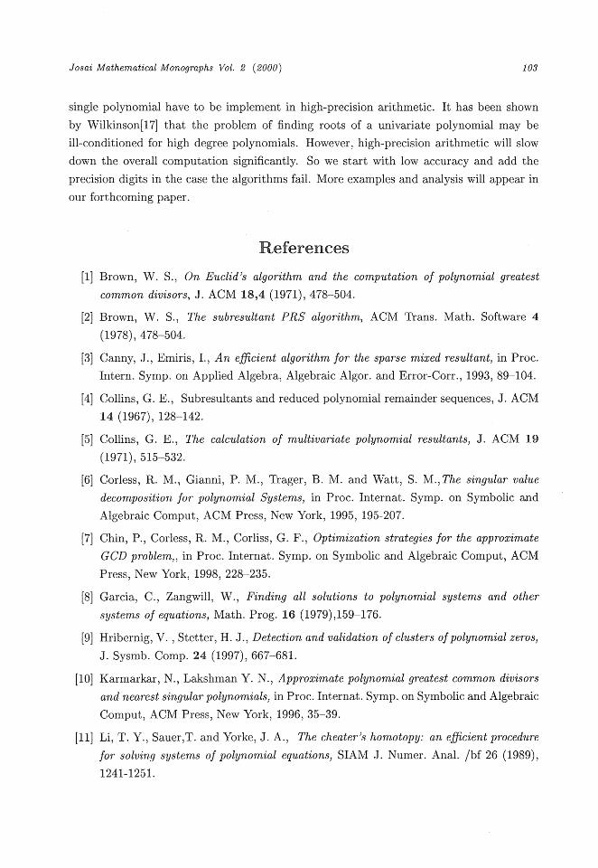
single polynomial have to be implement in high-precision arithmetic. It has been shown
by Wilkinson[17] that the problem of finding roots of a univariate polynomial may be
ill-conditioned for high degree polynomials. However, high-precision arithmetic will slow
down the overall computation signiflcantly. So we start with low accuracy and add the
precision digits in the case the algorithms fail. More examples and analysis will appear in
our forthcoming paper.
[1]
[2]
[3]
[4]
[5]
[6]
[7]
[8]
[9]
[10]
[1l]
ReferenceS
Brown, W. S.? On Euclid's algorithm and the computation of polynomial greatest
common divisors, J. ACM 18,4 (1971)) 478504.
Brown, W. S., The subresultant PRS algorithm, ACM Trans. Math. Software 4
(1978), 478-504.
Canny, J., Emiris, I., An efficient algorithm for the sparse mixed resultant, in Proc.
Intern. Symp. on Applied Algebra) Algebraic Algor. and Error-Corr., 1993, 89-104.
Collins, G. E.) Subresultants and reduced polynomial remainder sequences, J. ACM
14 (1967), 128-142.
Collins, G. E., The calculation of multivariate polynomial resultants, J. ACM 19
(1971), 515532.
Corless, R. M., Gianni, P. M., Trager, B. M. and Watt, S. M.,The singular value
decomposition for polynomial Systems, in Proc. Internat. Symp. on Symbolic and
Algebraic Comput, ACM Press, New York, 1995, 195-207.
Chin) P., Corless, R. M., Corliss, G. F., Optimization strategies for the approximate
GCD problem,, in Proc. Internat. Symp. on Symbolic and Algebraic Comput, ACM
Press) New York, 1998) 228235.
Garcia, C., Zangwill, W., Finding all solutions to polynomial systems and other
systems of equations; Math. Prog. 16 (1979),159-176.
Hribernig, V. , Stetter, H. J., Detection and validation of clusters of polynomial zeros,
J. Sysmb. Comp. 24 (1997)) 667681.
Karmarkar, N., Lakshman Y. N., Approximate polynomial greatest common divisors
and nearest singular polynomials, in Proc. Internat. Symp. on Symbolic and Algebraic
Comput, ACM Press, New York, 1996, 35-39.
Li, T. Y., Sauer,T. and Yorke, J. A.) The cheater's homotopy: an efficient procedure
for solving systems of polynomial equations, SIAM J. Numer. Anal. /bf 26 (1989))
1241-1251.
10A Procedings of NLA99 (2000)
[ 1 2]
[13]
[14]
[15]
[16]
[17]
[ 1 8]
[19]
[20]
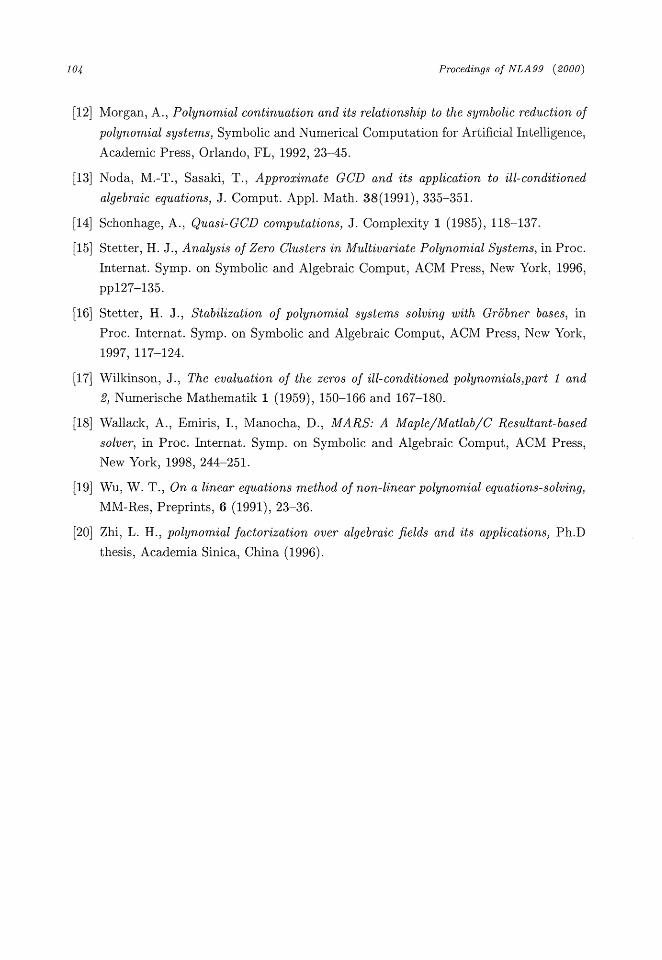
Morgan, A., Polynomial continuation and its relationship to the symbolic reduction of
polynomial systems, Symbolic and Numerical Computation for Artificial Intelligence,
Academic Press, Orlando, FL, 1992, 23-45.
Noda, M.-T., Sasaki, T., Approximate GCD and its application to ill-conditioned
algebraic equations, J. Comput. Appl. Math. 38(1991), 335351.
Schonhage, A., Quasi-GCD computations, J. Complexity I (1985), 118-137.
Stetter, H. J., Analysis of Zero Clusters in Multivariate Polynomial Systems, in Proc.
Internat. Symp. on Symbolic and Algebraic Comput, ACM Press, New York, 1996,
ppl27-135.
Stetter, H. J., Stabilization of polynomial systems solving with Gr6bner bases, in
Proc. Internat. Symp. on Symbolic and Algebraic Comput, ACM Press, New York,
1997, 117-124.
Wilkinson. J., The evaluation of the zeros of ill-conditioned polynomials,part I and
2, Numerische Mathematik I (1959), 150-166 and 167-180.
Wallack, A., Emiris, I., Manocha. D., MARS: A Maple/Matlab/C Resultant-based
solver, in Proc. Internat. Symp. on Symbolic and Algebraic Comput, ACM Press,
New York, 1998, 244-251.
Wu, W. T., On a linear equations method of non-linear polynomial equations-solving,
MM-Res, Preprints, 6 (1991), 23-36.
Zhi, L. H., polynomial factorization over algebraic fields and its applications, Ph.D
thesis, Academia Sinica, China (1996).