Hybrid Control for Topologically Constrained Systems€¦ · Hybrid Control for Topologically Constrained Systems A Dissertation submitted in partial satisfaction of the requirements

UNIVERSITY of CALIFORNIA

Santa Barbara

Hybrid Control for Topologically ConstrainedSystems

A Dissertation submitted in partial satisfaction of the

requirements for the degree

Doctor of Philosophy

in

Electrical and Computer Engineering

by

Christopher G. Mayhew

Committee in charge:

Professor Andrew R. Teel, Chair

Professor Joao P. Hespanha

Professor Roy Smith

Professor Francesco Bullo

December 2010

The dissertation of Christopher G. Mayhew is approved.

Professor Joao P. Hespanha

Professor Roy Smith

Professor Francesco Bullo

Professor Andrew R. Teel, Committee Chair

November 2010

Hybrid Control for Topologically Constrained Systems

Copyright c© 2010

by


iii

To Jean and Evan.

iv

Curriculum Vitæ


Education

2005 B.S. Electrical Engineering, Univeristy of California, River-

side.

2008 M.S. Electrical and Computer Engineering, University of

California, Santa Barbara.

Experience

2010–present Researcher at Robert Bosch LLC Research and Technology

Center, Palo Alto, California.

2006–2010 Graduate Student Researcher at University of California,

Santa Barbara.

2008 Engineering Intern at Robert Bosch LLC Research and Tech-

nology Center, Palo Alto, California.

2005–2006 Teaching Assistant at University of California, Santa Bar-

bara.

Selected Publications

C. G. Mayhew, R. G. Sanfelice, and A. R. Teel, “Robust global asymptotic atti-

tude stabilization of a rigid body by quaternion-based hybrid feedback,” in Pro-

ceedings of the 48th IEEE Conference on Decision and Control and 28th Chinese

Control Conference, 2009, pp. 2522–2527.

v

C. G. Mayhew, R. G. Sanfelice, and A. R. Teel, “Robust global asymptotic sta-

bilization of a 6-DOF rigid body by quaternion-based hybrid feedback,” in Pro-

ceedings of the 48th IEEE Conference on Decision and Control and 28th Chinese


C. G. Mayhew, R. G. Sanfelice, M. Arcak, and A. R. Teel, “Robust global asymp-

totic attitude synchronization by hybrid control,” in Proceedings of the American


C. G. Mayhew and A. R. Teel, “Global asymptotic stabilization of the inverted

equilibrium manifold of the 3D pendulum by hybrid feedback,” in Proceedings of

the 49th IEEE Conference on Decision and Control, 2010, to appear.

C. G. Mayhew, R. Sanfelice, and A. Teel, “Robust source-seeking hybrid con-

trollers for autonomous vehicles,” in Proceedings of the American Control Con-

ference, 2007, pp. 1185–1190.

C. G. Mayhew, R. Sanfelice, and A. Teel, “Robust source-seeking hybrid con-

trollers for nonholonomic vehicles,” in Proceedings of the American Control Con-

ference, 2008, pp. 2722–2727.

C. G. Mayhew, R. Sanfelice, and A. Teel, “Robust hybrid source-seeking algo-

rithms based on directional derivatives and their approximations,” in Proceedings

of the 47th IEEE Conference on Decision and Control, 2008, pp. 1735–1740.

C. G. Mayhew, K. L. Knierim, N. A. Chaturvedi, S. Park, J. Ahmed, and A. Kojic,

“Reduced-order modeling for studying and controlling misfire in four-stroke hcci

vi

engines,” in Proceedings of the 48th IEEE Conference on Decision and Control

held jointly with the 28th Chinese Control Conference, 2009, pp. 5194–5199.

C. G. Mayhew and A. R. Teel, “Hybrid control of planar rotations,” in Proceedings

of the American Control Conference, 2010, pp. 154–159.

C. G. Mayhew and A. R. Teel, “Hybrid control of spherical orientation,” in Pro-

ceedings of the 49th IEEE Conference on Decision and Control, 2010, to appear.

vii

Abstract

Hybrid Control for Topologically Constrained Systems

by


The topology of the configuration manifold for many physical systems is inherently

troublesome from a control perspective. In fact, for systems having a compact con-

figuration manifold, there exists no continuous control law that is globally asymp-

totically stabilizing for some desired equilibrium point in the manifold. Memory-

less discontinuous state feedback control is sometimes employed to “solve” such

topological issues; however, we show that global attractivity properties brought

about by such controllers are not robust to arbitrarily small measurement noise.

In this work, we employ hybrid control to solve the robust global stabilization

problem for such topologically constrained systems. In particular, we propose a

control scheme that coordinates a family of Lyapunov-based control laws using

state-based hysteretic switching. Using Lyapunov functions to generate the family

of control laws instantly yields a condition on the family of Lyapunov functions

that is equivalent to guaranteeing robust global asymptotic stability of the closed-

loop system. Hence, with the proposed hybrid controller, the original robust global

stabilization problem is transformed into one of finding a family of “synergistic”

Lyapunov functions. While this problem is difficult in general, we provide some

viii

results for manifolds commonly encountered in engineering including the unit

circle, unit 2-sphere, and the special orthogonal group of order three.

In many cases, the topological complexity of certain manifolds can be reduced

by considering its representation in a “covering space.” While this transformation

makes certain aspects of a control design less difficult, it introduces some subtleties

that are often ignored and can have very undesirable consequences for the closed-

loop system. We carefully examine rigid body attitude control in the context

of a quaternion representation and again provide a hybrid control scheme that

provides robust global asymptotic tracking and synchronization of a network of

rigid bodies.

ix

List of Symbols

Notation

• N denotes the natural numbers, i.e. N = 0, 1, 2, . . . .

• Z denotes the integers.

• R, R≥0, and R≤0 denote the real, nonnegative, and nonpositive real numbers,

respectively.

• Rn denotes n-dimensional real numbers with canonical basis vectors e1, . . . , en.

• Rn×m denotes the set of real-valued n×m matrices.

• Given x ∈ Rn×1 or X ∈ R

n×m, x⊤ ∈ R1×n, respectively, X⊤ ∈ R

m×n denotes

its transpose.

• Given a matrix A ∈ Rn×n, trace(A) is the sum of its diagonal entries, det(A)

denotes the determinant of A.

• Given vectors x, y ∈ Rn, or matrices A,B ∈ R

n×n, their natural inner

product is denoted 〈x, y〉 = x⊤y or 〈A,B〉 = traceA⊤B, respectively.

• Given x ∈ Rn, its Euclidean norm is |x| =

√〈x, x〉.

x

• Given A ∈ Rm×n, its Frobenius norm is |A|F =

√〈A,A〉.

• The set Sn = x ∈ R

n+1 : |x| = 1 is the n-dimensional unit sphere embed-

ded in Rn+1.

• B = x ∈ Rn : |x| ≤ 1 is the closed unit ball in Euclidean space.

• Given a set S, its closure is S, its interior is S, and its boundary is ∂S.

• Given a set S ⊂ Rn, convS and convS denote its convex hull and closed

convex hull, respectively.

• Given a set S ⊂ Rn and x ∈ R

n, |x|S = infy∈S |x− y|.

• Given sets S1, S2 ⊂ Rn, S1 + S2 = x1 + x2 : x1 ∈ S1, x2 ∈ S2.

• Given a matrix A ∈ Rm×n, its ijth element is Aij.

• Given a matrixA ∈ Rm×n, its vectorization is vecA =

[(Ae1)

⊤ · · · (Aen)⊤]⊤

.

• The vector of ones is 1 =

[1 · · · 1

]⊤.

• Given matrices A ∈ Rm×n and B ∈ R

p×q, their Kronecker product is the

mp× nq matrix.

A⊗B =

A11B · · · A1nB

.... . .

...

Am1B · · · AmnB

. (0.1)

• Given a matrix A ∈ Rn×n, its exponential is the matrix

expA = eA =∞∑

k=0

1

k!Ak. (0.2)

xi

• The set SO(n) = X ∈ Rn×n : X⊤X = XX⊤ = I, detX = 1 is the special

orthogonal group of order n. Its Lie algebra is the set so(n) = S ∈ Rn×n :

S⊤ = −S.

• Given a matrix A ∈ Rn×n, its projection onto so(n) is given by the operator

skew : Rn×n → so(n), defined as

skewA =A− A⊤

2. (0.3)

• Given y, z ∈ R3, their cross product is y × z = [y]× z, where

[y]× =

0 −y3 y2

y3 0 −y1

−y2 y1 0

. (0.4)

The map vec× : so(3) → R3 is the inverse of [·]×, that is,

vec× [y]× = y. (0.5)

• A continuous function α : R≥0 → R≥0 is said to be class-K if α(0) = 0 and

it is strictly increasing.

• A function α : R≥0 → R≥0 is said to be class-K∞ if it is class-K and

lims→∞ α(s) = ∞.

• A continuous function β : R≥0 × R≥0 → R≥0 is said to be class-KL if for

each fixed r, the map s 7→ β(s, r) is class-K and if for each fixed s, the map

r 7→ β(s, r) is decreasing and limr→∞ β(s, r) = 0.

• Given a topological space X, the set of all subsets of X is 2X . Given a

toplogical space Y , a set-valued map F : X → 2Y is denoted F : X Y .

xii

• Given topological spaces X, Y , and a set-valued map F : X Y , the

domain, range, and graph of F are the sets

domF = x ∈ X : F (x) 6= ∅,

rgeF = y ∈ Y : ∃x ∈ X such that y ∈ F (x),

gphF = (x, y) ∈ X × Y : y ∈ F (x).

xiii

Contents

Curriculum Vitæ v

Abstract viii

List of Symbols x

1 Introduction 1

1.1 Topological Compatibility of Control Objectives and the State Space 2

1.2 Potential-Based Control of Mechanical Systems . . . . . . . . . . 5

1.3 Potential Functions and Manifold Topology . . . . . . . . . . . . . 9

1.4 Synergistic Potential Functions and Hybrid Control . . . . . . . . 12

1.5 Quaternion-Based Control of Rigid-Body Attitude . . . . . . . . . 15

2 Topological Obstructions to Robust Global Asymptotic Stability 18

2.1 Continuous Dynamical Systems . . . . . . . . . . . . . . . . . . . 19

2.2 Differential Inclusions . . . . . . . . . . . . . . . . . . . . . . . . . 23

3 Hybrid Control with Synergistic Potential Functions 34

3.1 Background . . . . . . . . . . . . . . . . . . . . . . . . . . . . . . 35

3.1.1 The Lusternik-Schnirelmann Category . . . . . . . . . . . 35

3.1.2 Basic Results from Morse Theory . . . . . . . . . . . . . . 37

3.2 Synergistic Potential Functions and Hybrid Control . . . . . . . . 43

3.3 Control of Planar Rotations in S1 . . . . . . . . . . . . . . . . . . 51

xiv

3.3.1 Problem Statement and Notation . . . . . . . . . . . . . . 52

3.3.2 Hybrid Control Structure . . . . . . . . . . . . . . . . . . 54

3.3.3 Synergistic Potentials for S1 via Angular Warping . . . . . 57

3.4 Control of Spherical Orientation in S2 . . . . . . . . . . . . . . . . 61


3.4.2 Hybrid Control Structure . . . . . . . . . . . . . . . . . . 65

3.4.3 Synergistic Potentials for S2 via Angular Warping . . . . . 67

3.4.4 Global Asymptotic Stabilization of the Inverted EquilibriumManifold of the 3-D Pendulum . . . . . . . . . . . . . . . . 71

3.5 Control of Rigid Body Attitude in SO(3) . . . . . . . . . . . . . . 82


3.5.2 Hybrid Control Structure: Kinematics & Dynamics . . . . 88

3.5.3 Not-So-Synergistic Potential Functions on SO(3) . . . . . . 93

3.5.4 Synergistic Potentials for SO(3) via Angular Warping . . . 98

3.5.5 Simulation Results . . . . . . . . . . . . . . . . . . . . . . 101

4 Quaternion-Based Attitude Control 111

4.1 Disambiguation . . . . . . . . . . . . . . . . . . . . . . . . . . . . 114

4.1.1 Inconsistent Quaternion-based Control Laws and Path Lifting116

4.1.2 A Hybrid Algorithm for Dynamic Path Lifting . . . . . . . 125

4.1.3 The Unwinding Phenomenon . . . . . . . . . . . . . . . . 131

4.2 Kinematic Attitude Stabilization . . . . . . . . . . . . . . . . . . 135

4.3 Quaternion-Based Tracking Control . . . . . . . . . . . . . . . . . 144

4.3.1 Tracking Error Dynamics . . . . . . . . . . . . . . . . . . . 145

4.3.2 Hybrid Attitude Tracking Controller . . . . . . . . . . . . 147

4.3.3 Simulation Study . . . . . . . . . . . . . . . . . . . . . . . 161

4.4 Attitude Synchronization . . . . . . . . . . . . . . . . . . . . . . . 163

4.4.1 Multi-Agent Framework . . . . . . . . . . . . . . . . . . . 165

4.4.2 Relative Attitude Error Coordinates and the Synchroniza-tion Problem . . . . . . . . . . . . . . . . . . . . . . . . . 167

4.4.3 Robustly Synchronizing Hybrid Controller . . . . . . . . . 170

xv

4.4.4 The Hybrid Controller . . . . . . . . . . . . . . . . . . . . 170

4.4.5 The Closed-Loop System . . . . . . . . . . . . . . . . . . . 173

4.4.6 Simulation Study . . . . . . . . . . . . . . . . . . . . . . . 179

5 Conclusion 189

5.1 Summary . . . . . . . . . . . . . . . . . . . . . . . . . . . . . . . 189

5.2 Future Directions . . . . . . . . . . . . . . . . . . . . . . . . . . . 190

A Hybrid Systems Framework 193

B Topology 197

C Calculus, Manifolds, and Differential Geometry 207

D Matrix Calculus by Vectorization and the Kronecker Product 213

E Properties of the Cross Product 216

F Proofs 220

F.1 Proof of Theorem 2.1.2 . . . . . . . . . . . . . . . . . . . . . . . . 220

F.2 Proof of Lemma 2.1.7 . . . . . . . . . . . . . . . . . . . . . . . . . 221


F.4 Proof of Lemma 2.2.9 . . . . . . . . . . . . . . . . . . . . . . . . . 222






F.10 Proof of Lemma 3.5.5 . . . . . . . . . . . . . . . . . . . . . . . . . 231





xvi


F.16 Proof of Lemma 4.1.8 . . . . . . . . . . . . . . . . . . . . . . . . . 246





Bibliography 263

xvii

Chapter 1

Introduction

On a sunny Thursday afternoon in University of California, Santa Barbara,

two students are walking to their next destination, merrily ignorant of their inter-

twined fate: a catastrophic collision that would disrupt the chronology of a fresh

set of class notes and leave one cellular phone completely destroyed. From the

Arts building, an ECE student departs from a graduate mathematics course and

heads eastbound for Phelps Hall, where a nonlinear analysis course awaits to re-

lieve the student’s preoccupation of how a strictly increasing continuous function

could possibly have a derivative of zero. On the other side of campus, an under-

graduate Psychology major departs from Campbell hall, largely unconcerned with

the lecture on Pavlovian conditioning and is instead, engaged in a cell phone con-

versation regarding the coming night’s events. As their paths converge in front of

the Arbor, neither student is so much concerned with the immediate path ahead

until, within a small distance of one another, both students sense the impending

collision and take evasive action. Left and right, the students counter each other’s

movements until they inevitably meet in a not-so-elastic collision, sending cell

1

phone, measure theory, and students in all directions, yet reuniting soon after at

a common potential energy.

In the aftermath, the ECE student cannot help but analyze the conditions

leading to the accident and wonder if it could have been avoided. Upon a close

investigation, the student decomposes the situation into three pieces: a goal, a

constraint, and an algorithm. The goal was to move from point A to point B. The

constraint was that the path taken from A to B could not intersect the path of an

undergraduate psychology student at the same point in time. The algorithm was

supposed to steer the ECE student to the destination without collision and the

ECE student wondered if the collision was a result of a poor algorithm. Certainly,

a “smooth” algorithm could not be a “good” one, the student reckoned, as there

would be some intermediate point where the algorithm had to transition between

“move right” and “move left” around the obstacle. The student also noted that an

algorithm which transitioned very quickly was probably the algorithm used during

the accident, as small movements of the obstacle led to many abrupt changes in

the algorithm’s commanded direction, yielding a net translation of zero. Finally,

the student concluded that if only the algorithm had been decisive and insensitive

to the small changes in the obstacle’s position that the collision could have been

avoided.

1.1 Topological Compatibility of Control Objec-

tives and the State Space

A common objective in control engineering is to develop an algorithm that

consistently delivers a desired objective in the face of constraints. While various

2

constraints arise in many applications, the constraints arising in the introductory

story impart a fascinating difficulty to achieving the desired objective. In this

situation of obstacle avoidance, the student was not able to move about in the

environment freely, yet had to achieve the goal of arriving to the next class. In

this example, the constrained environment and the desired objective were not

topologically compatible. Let me clarify.

A wide range of control systems can be modeled by a differential equation

x = f(x, u) x ∈ X , (1.1)

where the state x is constrained to evolve within some state space X and u is a

vector of control inputs in some admissible control space U . In this scenario, many

control objectives can be cast as achieving asymptotic stability of a compact set

A ⊂ X . That is, the control designer must produce an algorithm κ : X → U

such that the resulting feedback system defined by setting u = κ(x) steers points

in X to A and keeps them close to A upon arrival. This requires that for a

neighborhood U of points around A, the direction of f(x, κ(x)) point inwards

towards A. Perhaps most desirable would be if f(x, κ(x)) could steer all points

in X to A. Going backwards in time, this would require that the differential

equation (1.1) take the neighborhood U and deform it so that it “fills up” X . But

what if U and X aren’t the same shape? That is, what if U and X do not have

the same topological structure? In this case, the differential equation (1.1) might

need to cut holes in U or glue pieces of it together so that it matches the shape

of X . As it turns out, these are not things that differential equations can do, at

least under the assumption of continuity [1–3].

3

At this point, one might wonder if it is possible for a discontinuous differential

equation to produce the desired result. That is, will a discontinuous differential

equation be able to cut and paste the neighborhood U so that its shape matches

the state space? Of course, one then has to ask, what is a solution to a differential

equation with a discontinuous right-hand side and how are solutions dependent

on changes in initial conditions? These questions have been studied in great

detail over the years and answered in [4–8], for example. While many notions of

solutions to discontinuous differential equations exist in the literature, the notion

we persist in using in this work (studied by the aforementioned references) is

known as a Krasovskii solution. By definition, this notion of solution leads to

studying absolutely continuous solutions of a differential inclusion

x ∈ F (x) x ∈ X (1.2)

that satisfies certain regularity properties.

The basic reason for studying these solutions is that they capture all solutions

of a discontinuous differential equation that can be brought about by arbitrar-

ily small measurement noise [4, 5, 9, 10]. Thus, studying asymptotic stability for

such differential inclusions is equivalent to studying robust stability of the original

discontinuous differential equation. The main result of Chapter 2 is that asking

for robust global asymptotic stability of some compact set A ⊂ X under the ac-

tion of (1.2) (satisfying certain regularity properties) implies the existence of a

smooth differential equation that renders A globally asymptotically stable. As

an unfortunate consequence, this implies that, even if one is willing to relax the

admissible feedback control algorithm to be discontinuous, it may be impossible

to robustly and globally stabilize a compact set that does not have the same topo-

4

logical structure as the state space. Returning a final time to our introductory

story, we see that the ECE student’s obstacle avoidance algorithm was probably

a discontinuous one and very sensitive to changes in the measured position of

inbound undergrads, which caused the chattering collision-bound trajectory.

While we do not examine a solution to the obstacle avoidance problem in this

work, we do examine several systems that evolve on a constrained state space,

where the stabilization goal is not topologically compatible with the state space.

In particular, we examine systems evolving on a compact manifold, like the unit

circle. It is easy to see that a small neighborhood around a point in the unit circle

is topologically equivalent to a small line segment; however, the unit circle, as a

whole is not topologically equivalent to a line segment, without gluing the ends of

the line segment together. These nonlinear state spaces arise naturally, especially

in systems with rotational degrees of freedom. These types of systems are the

primary focus of this dissertation.

1.2 Potential-Based Control of Mechanical Sys-

tems

A simple mechanical system consists of a smooth Riemannian manifold, a

smooth Lagrangian corresponding to kinetic energy minus potential energy, and

a set of external forces [11, 12]. When a subset of these forces are available for

control, the result is a simple mechanical control system [13–18]. While it is out

of the scope of this dissertation to consider the global stabilization of mechanical

systems in a broad generality, we provide a brief historical overview. General

references for classical mechanics and dissipative mechanical systems are [12, 16,

5

19]. A control-oriented perspective of mechanical systems is given in [15].

Many problems in control systems are specified as the stabilization of a de-

sired configuration of a mechanical system, prompting a vast literature concern-

ing the stabilization of specific or general mechanical systems. Applications come

in the form of autonomous vehicles [20–23] (underwater and otherwise), robotic

manipulators [24–26], satellites [27, 28], pendulum systems [29–32], quad-rotor

aircraft [33,34], and gimbal-based pointing mechanisms [35–37], to name a few.

In classical mechanics, the work done on a particle x ∈ R3 by a force F : R

3 →

R3 as the particle moves along a curve C, is calculated as the integral

W =

∫

C

F (p)dp =

∫ 1

0

〈F (p(t)), p′(t)〉 dt,

where p : [0, 1] → R3 is an arbitrary parametrization of the curve C. When

this integral is dependent only on the endpoints of the path, p(0) and p(1), and

independent of the actual path taken to and from the endpoints, the force is

said to be conservative [38, 39]. By a result of elementary calculus [40, §7.4] this

condition is equivalent to expressing the force F as the negative gradient of some

scalar function P : R3 → R. That is,

F = −∇P.

The function P is often called a potential function and is a measure of the po-

tential energy, or the stored energy of position due to F . Often, potential energy

exists in a system due to basic physical phenomena, like the force exerted by the

deformation of a spring or the force due to mass and gravity, but in a controlled

system, we, the control designers, have the opportunity to shape the potential

6

energy of the system or even inject and remove energy in the system through

actuation.

The analysis and control of mechanical systems from an energy viewpoint has

been present for some time. In fact, it has been known for centuries that dissi-

pative mechanical systems converge to a local minimum of a potential function.

Early works include [41], where Lagrange investigated the stability of motion

about equilibrium states of a conservative system. Later, [42] showed that the

introduction of dissipative forces lead to asymptotic stability of local minima of

potential function. Lyapunov later generalized these ideas in [43], which gained a

wide acceptance after being introduced to the control community in [44].

As these ideas gained in popularity, the idea of creating an artificial potential

energy through control action took hold in the robotics community for control

of robotic manipulators, arguably first in [45]. These ideas were followed by

[26,46], which explicitly incorporated an artificial potential energy into the control

strategy. Similar ideas were pursued in [47]. Introducing an artificial potential

energy soon became useful for obstacle avoidance in robotic manipulation and

vehicular navigation as well, with the first work appearing in [48], closely followed

by [49] and [22,50–52].

As the applications in robotics grew rapidly, the ideas were soon applied to

generalized notions of mechanical control systems using methods of differential

geometry. Some of the first work appeared in [53] for mechanical systems in

Hamiltonian form, where a potential shaping control was applied to conclude

local asymptotic stability of an equilibrium point. Later, generalized PD control

mechanical systems was studied in [54] and a strict Lyapunov function was found

for systems evolving on a configuration manifold with a trivial (parallelizable)

7

tangent bundle. The same author extended this analysis to mechanical systems

in a Lagrangian framework in [13], where global conclusions were drawn about

the solutions to dissipative mechanical systems using total energy (potential plus

kinetic) as a Lyapunov function. At the same time, a tracking result appeared

for fully actuated mechanical systems in a Lagrangian framework [14], though no

global conclusions were drawn.

In the last decade, artificial energy considerations in control were further ad-

vanced. The work of [55], followed up by many of the same authors in [56] and [57]

investigated the role of potential functions in the context of Hamiltonian systems

and exploited their inherent passivity properties. At the same time, the idea of

shaping potential functions for Lagrangian systems appeared in [58]. Most re-

cently, the work of [11, 59] provides for tracking, and stabilization of Lagrangian

systems evolving on Lie groups and stabilization in the case of output feedback.

However, the results in [11, 59] lead to a control law that cancels many benign

nonlinearities. In contrast, the recent work in [18,60] gives control laws for almost

global stabilization of mechanical systems evolving on a general Riemannian man-

ifold, even in the face of actuator saturation. In [18,60], the resulting control law

does not cancel benign nonlinearities and relies completely on the construction of

a suitable potential function and a choice of damping-injection function.

While the results mentioned above have been instrumental in designing feed-

back control laws for a broad class of nonlinear mechanical systems, all of them

rely on a smooth feedback strategy constructed from a single potential function

and an additional term that removes energy from the system. Since it is known

that this control structure forces the system to converge to the set of critical points

of a potential function and leads to asymptotic stability of the set of local minima

8

of the potential function, one might wonder if it is possible to design potential

functions on a given manifold with only one critical point: a global minimum at

the desired equilibrium. A deeper look into this problem reveals that this goal is

not possible in general, due to the topological structure of the underlying state

space.

1.3 Potential Functions and Manifold Topology

Given a smooth scalar-valued function defined on a manifold, one can ask very

basic questions about its critical behavior. How many critical points does it have

and where do they lie? Is a given critical point a local minimum, maximum, or

a saddle point? Further, one can ask that a scalar-valued function satisfy some

desirable properties. Does it have only one local minimum, which is a global

minimum? Are the critical points isolated, or do they form a connected subset?

As it turns out, these questions probe at a deep topological level and were answered

to a great extent in the 1930’s, largely by L. Lusternik, L. Schnirelmann, and M.

Morse.

In 1934, Lusternik and Schnirelmann used the notion of category, or Lusternik-

Schnirelmann category (LS category) as it came to be known, to form a lower

bound for the number of critical points of any smooth function on a manifold. In

its original definition (and the one we will persist in using in this dissertation), the

LS category is the minimal number of contractible sets needed to cover a manifold.

In [61], Lusternik and Schnirelmann proved that this topological invariant provides

a lower bound for the number of critical points for any smooth function defined on

a manifold. This work was revisited in [62], where the LS category of a manifold

9

was compared with more standard objects in topology. The LS category of many

manifolds, including the primary ones studied in this dissertation were calculated

in [63, 64]. Finally, while the LS category of a manifold establishes a hard lower

bound for the number of critical points of a smooth scalar-valued function on a

manifold, its broad applicability dulls its usefulness when functions are assumed

to have more structure.

At the same time Lusternik and Schnirelmann published [61], Marston Morse

published [65], whose basic ideas have been distilled and updated in various texts

over the years [66–68]. The resulting “Morse theory” allows one to directly study

the topology of a manifold through a particular (yet quite general) class of smooth

functions (termed “Morse functions”), their level sets, and their critical points.

Formally, a Morse function does not have any “degenerate” critical points where

its differential vanishes along with the nonsingularity of its Hessian matrix. A

result of this assumption is that critical points are isolated.

Most relevant to this dissertation are the results on the number and form

of critical points of a smooth Morse function. Indeed, when designing potential

functions for use in controlling mechanical systems, the potential functions are

often assumed to be a Morse function as in [11, 13, 18, 59]. The Morse function

assumption facilitates global conclusions about the stability and attractivity of

desired equilibrium points. In particular, it allows one to conclude almost global

asymptotic stability of a desired equilibrium. The so-called “Morse polynomial”

characterizes the nature of critical points and affords a bound on the minimal

number of critical points as the sum of the Betti numbers. When applicable, this

bound can be much sharper than the LS category of a manifold.

In any case, the results of [61] and [65] shed light on why existing control

10

x2

x1

Figure 1.1. Uniform gravity acting on a particle constrained to move along acircle. The potential force has no effect on the particle at the top and bottom ofthe circle.

schemes on topologically troublesome manifolds fail to be global: there must be

more than one critical point for any scalar-valued function defined on the manifold.

This of course stems from the topological incompatibility of the control objective

(expressed by the potential function) and the state space. Consider, for example,

the situation shown in Figure 1.1. Here, a particle in a uniform gravity field is

constrained to move in a circle. At the top and bottom of the circle, the force

has no component that is tangent to the circle and so its effect on the particle

vanishes at these points.

In situations like the one in Figure 1.1, control actuation resulting from a

single potential function is not enough to guarantee global asymptotic stability,

as the influence of the force derived from a potential function can easily vanish

in places other than a desired equilibrium. Fortunately, this realization hints at a

possible solution, once one is willing to relax allowable feedback control strategies

to those that coordinate multiple control laws constructed from multiple potential

functions.

11

1.4 Synergistic Potential Functions and Hybrid

Control

A controller that coordinates a family of control laws constructed from a family

of potential functions requires them to work as a synergistic unit. At a bare

minimum, one requires that for each undesirable critical point (one that is not the

desired system state) of each potential function in the family, there exists another

potential function that doesn’t share this “bad” critical point. However, as we

show later by counter example, this is not a sufficient condition for guaranteeing

synergism, which, in this dissertation, requires that for each bad critical point of

each potential function in the family, there exists another potential function of

lower value. That is, there is always some “gap” between the minimum potential

function in the family and the critical values of all other potential functions in the

family away from the desired state.

Having a family of synergistic potential functions immediately suggests a

method for coordinating their resulting control laws: hysteretically choose the

control corresponding to the potential function of minimal value. This “min-

switch” hybrid control paradigm has appeared in the literature in various contexts

over the past two decades. In particular, an early application of this idea for im-

plementing hysteresis in adaptive control was presented in [69], which was made

scale independent in [70]. Later, [71] proposed this method (without hysteresis)

for multi-controller systems where it has been applied for the problem of swinging

up an inverted pendulum in [72] and for control of a double-tank system in [73]

(which suggests a similar form for the hysteresis used in this paper). Ideas related

to synergistic potential functions also appear in [74] where multiple Lyapunov

12

functions are proposed for analysis of switched and hybrid systems and in [75,76],

where a “min-projection” hybrid strategy was proposed for the stabilization of

switched nonlinear systems.

The importance of synergism is closely related to the capability of switching

between controllers in a way that leads to robust global asymptotic stability. As

we show in this dissertation, if the switching strategy is a static (i.e. memoryless)

function of the state, this results in a memoryless discontinuous feedback that

may be arbitrarily sensitive to measurement noise. So, always greedily using

the control law corresponding to the minimum potential function may not be a

robust strategy. However, the synergism property permits endowing a control-

coordination strategy with the virtue of patience via hysteresis, thanks to the gap

between the critical values of the potential functions away from the desired state.

That is, one can give memory to the control selection process so that it waits until

some minimal decrease condition is met.

Hybrid systems–those which allow both continuous flow and discrete jumps of

the state–provide an appropriate setting for design and analysis of a control-law

coordination strategy. The recent hybrid systems framework of [77, 78], devel-

oped in the context of robust stability, is especially relevant for our purpose, as

measurement-noise sensitivity can destroy global attractivity properties for mem-

oryless discontinuous feedback. This framework, reviewed in [78], posits a hybrid

system H with a state x ∈ Rn, possibly including both continuous and discrete

state components, as a collection of four objects: a flow map F : Rn

Rn that

governs continuous evolution of the state, a flow set C ⊂ Rn that dictates where

continuous evolution can occur, a jump map G : Rn

Rn that governs discrete

jumps of the state, and a jump set D ⊂ Rn that dictates where jumps can occur.

13

A hybrid system is written succinctly as H = (F,G,C,D), or

H

x ∈ F (x) x ∈ C

x+ ∈ G(x) x ∈ D.

Hybrid systems lend a very useful tool to deal with topologically constrained

control problems: the use of logic variables for implementing hysteresis and break-

ing topological constraints while retaining robustness. Consider again, the differ-

ential equation (1.1) and suppose that we had designed N controllers, κq : X → U

that, for each q ∈ 1, . . . , N, could be applied on the set Cq ⊂ X and that

⋃q∈1,...,NCq = X . When the sets Cq have some overlap, it is possible to design a

control strategy that adds memory (i.e. hysteresis) to the crucial decision of when

and how to switch control laws. In this situation, one might have the following

closed-loop system, where q becomes a memory state:

x = f(x, κq(x))

q = 0︸︷︷︸

x ∈ Cq

x+ = x

q+ ∈ g(x)︸︷︷︸x ∈ Dq.

The difficult question to answer here becomes how to design the sets Cq, Dq and

a switching rule g(x) that guarantees global asymptotic stability of a desired

compact set A ⊂ X . By employing a synergistic family of potential functions, we

provide the hysteretic “min-switch” construction in Chapter 3 that results in the

desired objective.

14

1.5 Quaternion-Based Control of Rigid-Body At-

titude

An important case study of the methods proposed in this dissertation is the

stabilization of rigid-body attitude. The rigid-body configuration space, SO(3),

is rife with topological difficulty. In particular, SO(3) is a boundaryless com-

pact manifold and hence, is not diffeomorphic to any vector space [2, 13]. This

simple fact precludes the existence of any continuous feedback control law that

globally asymptotically stabilizes a desired attitude [2,13]. Instead, many authors

(e.g. [11,13,30,79–84]) settle for almost global asymptotic stability on such topo-

logically constrained manifolds, where the desired (locally asymptotically stable)

equilibrium is attractive from all points in the state space except a nowhere dense

set of zero Lebesgue measure.

Indeed, these topological obstructions make their way into Lyapunov analysis

in the form of critical points (or critical manifolds) for potential functions. This

phenomenon is easily seen in the context of rigid bodies, where potential func-

tions on SO(3) are guaranteed by the Lusternik-Schnirelmann category and Morse

theory to have at least 4 critical points, some of which are clearly not desirable.

In Chapter 3.5, we provide a hybrid controller based in SO(3) that uses multiple

potential functions to accomplish the desired stabilization task.

The attitude of a rigid body is often parametrized to exploit inherent redun-

dancies in the rotation matrix description of SO(3); however, certain parametriza-

tions face further topological difficulties. As pointed out in [85], no three-parameter

parametrization of SO(3) is globally nonsingular (i.e., the map from representation

coordinates to SO(3) is not everywhere a local diffeomorphism). This creates an

15

inherent obstacle in achieving global asymptotic stability using control methods

based on Euler angles (e.g. pitch, roll, yaw), (modified) Rodrigues parameters,

and exponential coordinates, among others.

Pursuing a globally nonsingular parametrization, many authors (as well as the

author of this dissertation) employ unit quaternions, which evolve on the three-

dimensional unit sphere embedded in R4, denoted as S

3. This parametrization

is everywhere a local diffeomorphism, but uses four parameters, is subject to a

unit-norm constraint, and is two-to-one. This double covering of SO(3) by S3

transforms the stabilization task. Where the original control objective was to

globally asymptotically stabilize a single equilibrium point in SO(3), the double-

covering property translates the control objective in S3 to the global asymptotic

stabilization of a disconnected set of two antipodal points that represent the same

attitude. Not surprisingly, neither of these two control objectives are topologically

compatible with their respective state space.

When this double covering is neglected, the resulting controller can induce very

undesirable behavior. In particular, when one attempts to asymptotically stabilize

a single equilibrium point in S3, rather than both points corresponding to the

same attitude (e.g. [28,86–90]), the desired attitude becomes an equilibrium point;

however, it may be stable, or unstable, depending on the controller’s knowledge

of the quaternion representation! This behavior has been documented for decades

and is referred to as the unwinding phenomenon [2, 28,86].

In Chapter 4, we thoroughly investigate the unwinding phenomenon in the

context of how to implement quaternion-based control laws that are not well-

defined on SO(3) (they may take on one of two values). As a result, we make

an equivalence between solutions of the “lifted system” on S3 and a closed-loop

16

system that dynamically lifts paths from SO(3) to S3 for the use of quaternion-

based feedback laws. In essence, this result justifies carrying out analysis in the

covering space S3 for such control laws, which is a widely-accepted practice in the

existing literature. The results also show that a stability result obtained in the

covering space may not actually be desirable, as it induces unwinding.

In Chapter 4, we derive a quaternion-based hybrid controller for kinematic

rigid-body attitude stabilization. We extend this to the dynamic case in a track-

ing problem for full state feedback and two output feedback cases. Finally, we

conclude this dissertation by applying this method to synchronizing the attitude

of a network of rigid bodies.

17

Chapter 2

Topological Obstructions to

Robust Global Asymptotic

Stability

In this chapter, we study the topological properties of asymptotically sta-

ble attractors of continuous dynamical systems and differential inclusions. These

properties are crucial to understanding some fundamental limits of feedback con-

trol. In particular, we will find that when a specified objective of feedback control

does not have the same topological structure as world in which the dynamical

system evolves, the task may be impossible to carry out, at least robustly, with

certain types of feedback. To conduct this study, we will abstract the notion

of a continuous-time dynamical system to a mapping commonly referred to as a

flow. This is the approach taken, for example, in [1,2], and some of the following

material follows these references closely.

18

2.1 Continuous Dynamical Systems

Definition 2.1.1. Given a topological space X, a flow on X is a continuous map

Φ : X × R → X that satisfies

1. Φ(x, 0) = x for every x ∈ X (identity axiom),

2. Φ(Φ(x, t1), t2) = Φ(x, t1 + t2) (group axiom).

Given a flow, one can define two auxiliary maps by holding either the first or

second argument constant. Precisely, we say that given a flow Φ : X×R → X, its

t-flow is the map Φt : X → X defined as Φt(x) = Φ(x, t) and its x-solution is the

map Φx : R → X defined as Φx(t) = Φ(x, t). Note that, given a flow Φ, any two

t-flows Φt1 and Φt2 are homotopic, since Φ is continuous in t. Furthermore, when

X is path connected, any two x0-solutions of Φ are also homotopic. A crucial

property of flows is that the action of a t-flow is a homeomorphism for any t ∈ R.

Theorem 2.1.2. For every t ∈ R, the t-flow of a flow Φ is a homeomorphism of

X onto itself.

Proof. See Appendix F.1.

This abstraction encompasses many notions of a dynamical system. Several

examples are given in [1], but perhaps most importantly are the solutions of a

differential equation

x = f(x), (2.1)

where x ∈ Rn and f : R

n → Rn. When (2.1) produces solutions that are unique

(both forward and backward in time) and depend continuously on their initial

19

condition, one can think of a flow induced by f as a representation of the solution

set to (2.1), streamlined into a function.

Moving from (2.1) to its flow is fairly straightforward and there are various

ways to ensure the necessary properties. For example, when f is locally Lipschitz,

solutions are guaranteed to be unique, at least on a small interval, both forward

and backward in time [91, 92], and are continuous with respect to their initial

condition. Solutions to (2.1) that have a limited time domain of definition can

also be identified with solutions to a regularized version of (2.1) (see [1,93]). More

generally, one may also consider the flow induced by the integral curves of a vector

field on a manifold [15,94,95]. Thus, this treatment is sufficiently general for our

purpose.

From the flow viewpoint of a continuous-time dynamical system, we can make

several classical definitions of invariance, stability, and attractivity.

Definition 2.1.3. A set A ⊂ X is forward invariant (backward invariant) under

the flow Φ if Φ(A, t) ⊂ A for all t ∈ R≥0 (t ∈ R≤0). It is invariant if it is

both forward and backward invariant. An invariant point x ∈ X is called an

equilibrium.

Definition 2.1.4. A set A ⊂ X is stable under the flow Φ if for every open set

Uǫ ⊃ A, there exists an open set Uδ ⊃ A such that Φ(Uδ, t) ⊂ Uǫ for all t ∈ R≥0.

Definition 2.1.5. A set A ⊂ X is attractive under the flow Φ from B if for every

x ∈ B and every open set U ⊃ A, there exists T ≥ 0 such that Φ(x, t) ∈ U for all

t ≥ T . The basin of attraction of A under Φ is the union of all sets from which

A is attractive, denoted as BΦ(A).

Definition 2.1.6. A set A ⊂ X is asymptotically stable under the flow Φ if it is

20

stable and attractive from an open set containing A.

From these classical definitions, we can prove several useful topological prop-

erties of attraction basins of asymptotically stable equilibria X. The develop-

ment of results here follows [3] and the following result is a slight generalization

of [3, Lemma 5.9.12].

Lemma 2.1.7. If A ⊂ X is asymptotically stable under Φ, then for every x ∈

BΦ(A) and every open neighborhood U of A, there exists an open neighborhood

V ∋ x and some some T ∈ R≥0 such that V ⊂ BΦ(A) and such that for all y ∈ V ,

it follows that Φ(t, y) ∈ U for all t ≥ T . In particular, BΦ(A) is an open set.


While Lemma 2.1.7 doesn’t present an obstruction to global asymptotic sta-

bility (X is open by definition), the next result appeals to Lemma 2.1.7 to assert

that the basin of attraction of an equilibrium is contractible (see Definition B.13).

This result appears in [3] and in part of the proof of [2, Theorem 1].

Theorem 2.1.8. If x0 ∈ X is an asymptotically stable equilibrium, then BΦ(x0)

is contractible.


This result has far-reaching implications. As a necessary condition on the

topological structure of an attraction basin for an equilibrium point, this result

effectively rules out the possibility of global asymptotic stabilization by smooth

feedback for a wide variety of set point stabilization problems when the state space

is not contractible to a point. In particular, degree theory provides the following

21

result [96, Ex. 2.4.6] for manifolds (see Appendix C and Definitions C.30 and

C.34)

Lemma 2.1.9. Any compact manifold (without boundary) is not contractible.

Corollary 2.1.10. Any product space M1 ×M2, where M1 is a compact manifold

is not contractible.

Corollary 2.1.11. If M is a compact manifold, its tangent bundle, TM is not

contractible.

Lemma 2.1.9 and its corollaries rule out the possibility of achieving global

asymptotic stability by smooth time-invariant state feedback for compact mani-

folds, including Sn and SO(n). In particular, any mechanical system with a rota-

tional degree of freedom cannot be globally asymptotically stabilized by smooth

time-invariant state feedback. This particular obstruction to global asymptotic

stability was studied in detail in [2].

Theorem 2.1.8 can be further generalized in a useful manner. The next result

is from [1, Theorem 3.4] and [97, Theorem 2.2].

Theorem 2.1.12. If x0 ∈ X is an asymptotically stable equilibrium under Φ,

then BΦ(x0) is homeomorphic to Rn for some n ≥ 0.

As it turns out, Theorem 2.1.12 can be generalized even further for attractors

that have the structure of a submanifold. Not surprisingly, the following result

of [97, Theorem 3.4] states that attraction basins for compact submanifolds “look

like” a small open set about the attractor that captures its topological properties.

Theorem 2.1.13. If A is an asymptotically stable compact submanifold of M

under Φ : M × R → M , then BΦ(A) is diffeomorphic to an open tubular neigh-

borhood of A.

22

We refer the reader to Appendix C for a rigorous description of a tubular

neighborhood. Loosely speaking, one can think of the tubular neighborhood of a

submanifold A ⊂M as a region about A contained in M defined by extending A

in all directions normal to A, so long as those directions do not intersect.

Example 2.1.14. A tubular neighborhood of a finite set xii∈A ⊂ Rn is the set

x : |xi − x| < 12mini6=j |xi − xj|.

Example 2.1.15. A tubular neighborhood of Sn ⊂ R

n+1 is the set Rn+1 \ 0.

Theorem 2.1.13 and the examples show that when the state space does not

have the same topology as an asymptotically stable compact attractor, the basin

of attraction cannot possibly be the entire state space. This is a topological con-

straint due to the fact that the flow was assumed to be a continuous function,

which, paired with the identity and group axioms led to the flow being a homeo-

morphism.

One might wonder what would happen if the flow was allowed to be discontin-

uous, or perhaps, one attempted to use discontinuous feedback to stabilize a target

compact set. We investigate these issues in the context of differential inclusions

that satisfy certain regularity properties.

2.2 Differential Inclusions

In this section, we generalize the results of Section 2.1 to systems whose solu-

tions are not unique (the flow will be “upper semicontinuous” in the topology of

uniform convergence). In particular, we will investigate whether the topological

properties seen for attraction basins for continuous dynamical systems also apply

23

to the differential inclusion

x ∈ F (x) x ∈M (2.2)

where M is a manifold and for every x ∈ M , F (x) ⊂ TxM . By a slight abuse

of notation, we will write F : M TM . We will assume that (2.2) satisfies

the regularity properties assumed in [93, 98]. We now examine these regularity

properties as an extension of continuity for set-valued mappings.

One of the primary difficulties in dealing with set-valued mappings is the

notion of continuity [6, 99]. Consider the two equivalent notions of continuity for

functions in Theorem B.8: f−1(U) is open when U is open and f−1(V ) is closed

whenever V is closed. If one tries to define continuity of set-valued maps using

these definitions, they will no longer be equivalent [99, 100]. Instead, they lead

to separate notions of semicontinuity. In this dissertation, we will primarily be

concerned with a subset of these notions.

Definition 2.2.1. Let X and Y be topological spaces and let F : X Y be a

set-valued mapping. The map F is upper semicontinuous if for every x ∈ X and

every open neighborhood V ⊃ F (x), there exists an open neighborhood U ∋ x

such that F (U) ⊂ F (V ). The map F is said to be outer semicontinuous if its

graph is closed.

These definitions are closely related. We refer the reader to the commentary

in [100, Ch. 5] for a complete historical recollection of these definitions. We recall

the facts that are most relevant to this dissertation here.

Definition 2.2.2. Let X and Y be topological spaces. A set-valued map F :

X Y is locally bounded if for any compact set K ⊂ X, there exists a compact

24

set L ⊂ Y such that F (K) ⊂ L.

Theorem 2.2.3. Let X and Y be topological spaces. If a set-valued map F :

X Y is upper semicontinuous, then it is outer semicontinuous. Under the

additional assumption that F is locally bounded and has closed values, F is upper

semicontinuous if and only if F is outer semicontinuous.

Definition 2.2.4. A set-valued map F : M TM satisfies the basic conditions

on a subset S ⊂M if it is locally bounded on S, outer semicontinuous on S, and

for each x ∈ S, F (x) is nonempty, compact, and convex.

The basic assumptions arise from considering the robustness of stability. In

fact, in the theory of differential inclusions, the main conditions that provide for

the robustness of stability are the closedness of solution sets (limits of solutions

are solutions) and the upper semicontinuity of solutions with respect to initial con-

ditions and perturbations (every perturbed solution is close to some unperturbed

solution).

Considering solutions to (2.2) also includes considering generalized solutions

to discontinuous systems with right-hand sides that result in differential inclusions

that satisfy the basic conditions [98]. In particular, Krasovskii solutions examined

in [4] result in such differential inclusions, which are exactly the solutions that can

be induced by arbitrarily small amounts of measurement noise [4, 101]. Finally,

we remark that studying (2.2) allows us to determine whether some set A ⊂ Rn

can be robustly asymptotically stabilized for some nonlinear plant

x = f(x, u), (2.3)

where x ∈ M , f : M × U TM , and u ∈ U, is chosen to be some nonlinear

25

state feedback feedback κ : M → Rm that is locally bounded, but possibly not

continuous.

Definition 2.2.5. A function x : [0, T ] → M is a solution to (2.2) under F if it

is absolutely continuous and satisfies, for almost all t ∈ [0, T ],

x(t) ∈ F (x(t)).

A solution x : [0, T ) → M (0 < T ≤ ∞) is said to be maximal if it cannot be

extended. It is complete if it is defined on [0,∞).

Following [93], we will denote a solution to (2.2) under F starting at x ∈ M

as φF (x, t). The set of maximal solutions (respectively, solutions defined on [0, t])

to (2.2) under F starting from x ∈ M or in a set K ⊂ M is denoted as SF (x),

or SF (K) (respectively, S(x, t) or S(K, t)). An important property of solution

sets is that for fixed t, they are upper semicontinuous (in the topology of uniform

convergence) on M × [0, T ] when all solutions exist on [0, T ] and t ≤ T ( [8,

Theorem 7.1], [6, §2.2 Theorem 1], [7, Theorem 3.5.2]). We note that both [8,

Theorem 7.1] and [6, §2.2 Theorem 1] apply to M = Rn, but [7, Theorem 3.5.2]

is sufficiently general to treat the case of when M is a smooth manifold.

Theorem 2.2.6. If all solutions to (2.2) exist on [0, T ], then the map x 7→ SF (x, t)

is upper semicontinuous for each t ∈ [0, T ].

At times, we will assume that solutions are defined for all time, so we make

the following definition.

Definition 2.2.7. The differential inclusion (2.2) is forward complete if, for all

x ∈M , all solutions φ ∈ SF (x) are defined for all t ≥ 0. The differential inclusion

26

2.2 is backward complete if the differential inclusion is x ∈ −F (x) is forward

complete. The differential inclusion (2.2) is complete if it is both forward and

backward complete.

Analogous to the definition of a flow studied in the previous section, we note

the following property of solution sets to (2.2) under F . We define the following

set-valued version of the “flow” under F as

ΦF (x, t) = φ(x, t) : φ ∈ SF (x, t) =⋃

φ∈SF (x,t)

φ(x, t). (2.4)

Then, [8, Corollary 7.1] and [6, §2.2 Corollary 1] afford the following corollary to

Theorem 2.2.6.

Corollary 2.2.8. If all solutions to (2.2) exist on [0, T ], then the map x 7→

ΦF (x, t) is upper semicontinuous for each t ∈ [0, T ].

To complete the analogy, we have the following lemma, which states a semi-

group property of the map ΦF .

Lemma 2.2.9. Suppose that (2.2) is forward complete. Then, for x ∈ M and

t1, t2 ≥ 0, the set-valued flow ΦF under F satisfies

ΦF (x, 0) = x (2.5)

ΦF (ΦF (x, t1), t2) = ΦF (x, t1 + t2) (2.6)

and ΦF is upper semicontinuous on Rn × [0,∞).


27

Since solutions to (2.2) under F may not be unique, we will slightly compen-

sate our definitions of stability, attractivity, and the basin of attraction for the

differential inclusion (2.2), though they are mostly identical to our previous defi-

nitions. In particular, we will enforce stability and attractivity to be uniform over

the solution set.

Definition 2.2.10. A set A ⊂ M is stable under F if for every neighborhood

Uǫ ⊃ A, there exists a neighborhood Uδ ⊃ A such that ΦF (Uδ, t) ⊂ Uǫ for all

t ≥ 0.

Definition 2.2.11. A set A ⊂M is attractive under F from B if for every x ∈ B

and every open set U ⊃ A, there exists T ≥ 0 such that ΦF (x, t) ⊂ U for all

t ≥ T . The basin of attraction of A under F is the union of all sets from which

A is attractive, denoted as BF (A).

Definition 2.2.12. A set A ⊂M is asymptotically stable under F if it is stable

and attractive from an open set containing A.

When considering asymptotic stability of a compact attractor, it is often useful

to define a measure of closeness to the attractor on some open neighborhood.

Definition 2.2.13. Given a compact subset A ⊂ M and an open neighborhood

U of A, a continuous function ω : U → R≥0 is a proper indicator for A on U if

ω(x) = 0 if and only if x ∈ A, and, when ∂U 6= ∅, limx→∂U

ω(x) = ∞ and otherwise,

for each compact set K ⊂ R≥0, the set x ∈M : ω(x) ∈ K is compact.

Definition 2.2.14. Let A ⊂ Rn be a compact subset, let U be an open neigh-

borhood of A, and let ω : U → R≥0 be a proper indicator for A on U . A function

V : U → R≥0 is a smooth Lyapunov function for A on U if there exist class-K∞

28

functions αi, i = 1, 2, such that for all x ∈ U ,

α1(ω(x)) ≤ V (x) ≤ α2(ω(x))

and

maxw∈F (x)

〈∇V (x), w〉 ≤ −V (x).

Now, we combine some primary results of [93] on the existence of Lyapunov

functions to meet our needs. The following lemma is [93, Proposition 3].

Lemma 2.2.15. Suppose that F : Rn

Rn satisfies the basic conditions and that

A ⊂ Rn is compact. Then, the basin of attraction of A under F is open. That is,

BF (A) is an open set.

Theorem 2.2.16. Let F : Rn

Rn satisfy the basic conditions and suppose

that A ⊂ Rn is compact and asymptotically stable. Then, there exists a smooth

Lyapunov function for A on BF (A).

Proof. First, we let ω : BF (A) → R≥0 be a proper indicator for A on BF (A).

Such a proper indicator exists because A was assumed to be compact and BF (A)

is open by Lemma 2.2.15. Since A was assumed to be asymptotically stable,

this implies that the differential inclusion is “KL-stable with respect to (ω, ω) on

BF (A)” (see [93, Definition 6] and apply [93, Proposition 3]). Now, this implies

that the differential inclusion (2.2) is “backward completable by ω-normalization”

( [93, Definition 9]). Finally, by [93, Theorem 3], we have the desired result.

Theorem 2.2.16 provides a very useful corollary that we state here as a theorem.

In particular, Theorem 2.2.16 implies that there exists a flow on the basin of

29

attraction of a compact attractor under a set-valued mapping that satisfies the

basic conditions.

Theorem 2.2.17. Let F : Rn

Rn satisfy the basic conditions and let A be

an asymptotically stable compact set under F . Then, there exists a flow Φ :

BF (A) × R → BF (A) such that A is globally asymptotically stable under Φ.

Proof. By Theorem 2.2.16, there exists a smooth Lyapunov function V : BF (A) →

Rn for A on BF (A). We construct a flow on BF (A) with the desired properties

as follows.

Consider the differential equation

x = g(x) :=−∇V (x)

1 + |∇V (x)|2 . (2.7)

Since V is smooth, it follows that the solutions to (2.7) are unique, and continu-

ously depend on x ∈ BF (A). Now, consider the Lyapunov function V : BF (A) →

R≥0. We see that

〈∇V (x), g(x)〉 = −|∇V (x)|2/(1 + |∇V (x)|2),

which is negative for all x ∈ BF (A) \ A, so A is asymptotically stable with

basin of attraction BF (A). Moreover, this establishes that solutions to (2.7) are

forward complete, since the compact sub-level sets of V are invariant. Finally,

since 0 ≤ w/(1 + w) < 1 for any w ∈ R≥0, it follows that

〈∇V (x),−g(x)〉 = |∇V (x)|2/(1 + |∇V (x)|2) ≤ 1.

Since V (x) → ∞ if an only if x → ∂BF (A), this implies that (2.7) is backward

30

complete. This yields the solution set to (2.7) as a flow on B, with A a globally

asymptotically stable set (when the state space is B).

We now extend Theorem 2.2.17 to the case when M is a smooth manifold. To

accomplish this task, we invoke a recent converse Lyapunov theorem for hybrid

systems in [102], as it allows for the state to evolve within a relatively closed

constraint set in Rn.

Theorem 2.2.18. Let M be an embedded submanifold of Rn, let F : M TM

satisfy the basic conditions, and let A be an asymptotically stable compact set

under F . Then, there exists a flow Φ : BF (A) × R → BF (A) such that A is

globally asymptotically stable under Φ.

Proof. Since M is an embedded closed submanifold of Rn, we can construct the

following hybrid system.

HF =

x ∈ F (x) x ∈M

x+ = x x ∈ ∅.(2.8)

Since the jump set is empty, it is impossible for the system to jump. Therefore,

this hybrid system has only solutions starting from M that remain within M

for their maximal intervals of existence. In fact, it is easy to identify a one-to-

one correspondence between solutions to the differential inclusion x ∈ F (x) and

solutions to the hybrid system H. This implies that when A is asymptotically

stable under F with basin of attraction BF (A), the set B = BF (A) ∪ (Rn \M)

is the basin of attraction for A for solutions to H, as defined in [102]. Also, it

was shown in [102, Lemma 7.12] that B ⊂ Rn is open. With this said, we call

upon [102, Theorem 3.14] to note the existence of a smooth Lyapunov function

31

V : B → R≥0 and class-K∞ functions α1, α2 such that

α(ω(x)) ≤ V (x) ≤ α2(ω(x)) ∀x ∈ B

maxw∈F (x)

〈∇V (x), w〉 ≤ −V (x) ∀x ∈ B,

where ω : B → R≥0 is a proper indicator for A on B (since B is open). Now, since

V is smooth on B, which is an open neighborhood of BF (A) ⊂ B, the restriction

of V to BF (A) yields a smooth Lyapunov function for the original differential

inclusion x ∈ F (x). That is, V |BF (A) is a smooth function whose Lie derivative

with respect to F is negative, so long as x ∈ BF (A)\A. But then, one can define

a smooth vector field on on BF (A) as the negative gradient of V |BF (A) and again,

normalize the magnitude of this vector field to yield a flow on BF (A) that renders

A asymptotically stable as in the proof of Theorem 2.2.17.

This theorem has immediate corollaries stemming from the results of the pre-

vious chapter.

Corollary 2.2.19. Let F : M TM satisfy the basic conditions and let A ⊂M

be compact and asymptotically stable under F . If A is a singleton, then BF (A) is

homeomorphic to Rn and contractible. If A is a submanifold of M , then BF (A)

is homeomorphic to an open tubular neighborhood of A.

Proof. By Theorem 2.2.17, there exists a flow Φ : BF (A) × R → BF (A). Then,

Theorems 2.1.8, 2.1.12, and 2.1.13 provide the results.

This result gives a necessary condition on the topological properties of attrac-

tors for differential inclusions that satisfy the basic conditions. This allows us to

32

decide whether a given control objective, stated in terms of robustly and globally

asymptotically stabilizing a compact set, is possible. Certainly, when the state

space is not homeomorphic to an open tubular neighborhood of the given compact

set, it is impossible to robustly and globally stabilize this set with a memoryless,

even discontinuous, state-feedback control law. Such troublesome control objec-

tives include stabilizing a disconnected set of points in Rn, stabilizing a point on

Sn or SO(n) (or their tangent bundles), or stabilizing a set diffeomorphic to S

1

within SO(3). The latter example corresponds to reduced attitude stabilization of

a rigid body.

An interesting observation from these results is that relaxing control laws to

be time-varying and periodic does not improve attractivity properties for a control

objective that is topologically incompatible with the state space. This is because

we can write such a system as

x ∈ F (x, ξ)

ξ = Jξ

(x, ξ) ∈M × S

1, (2.9)

where J = [ 0 −11 0 ]. Since ξ is confined to endlessly rotate around S

1, any asymp-

totically stable compact attractor for (2.9) must be written as A× S1. Hence, if

A is not topologically compatible with M , robust global asymptotic stability of

A× S1 is not possible.

33

Chapter 3

Hybrid Control with Synergistic

Potential Functions

In this chapter, we will recall results from differential topology and Morse

theory that examine the topology of a manifold through a scalar-valued function

defined on the manifold and its critical points (the points where its gradient van-

ishes). We will find that many manifolds are intrinsically problematic from the

control point of view in the sense that any scalar-valued function defined on the

manifold is guaranteed to have a multiple critical points. When a control strategy

is based upon descending a single smooth potential function, it can easily get

stuck at its critical points. This creates the need to relax our control schemes and

consider discontinuous or hybrid feedback.

The hybrid control schemes presented in this chapter, for S1, S

2, and SO(3) are

based upon using control laws derived from a family of smooth potential functions

and a strategy to switch between them when necessary. The basic intuition behind

this scheme is that when the system nears a critical point of one potential function,

34

there is another potential function and its corresponding control law in our family

to which we can switch. In this way, the potential functions work as a synergistic

unit, providing for global asymptotic stability of a desired system configuration

in the face of measurement noise.

3.1 Background

Our study of potential-function-based control has a long history. In this sec-

tion, we will recall previous results concerning the relationship between functions,

their level sets, their critical points, and the topology of their domain. In what

follows, given a smooth manifold M and a function f : M → R, the differential

of f is denoted df , which is defined rigorously in Appendix C. The set of critical

points of f on M is

Crit f = x ∈M : df = 0. (3.1)

The number of critical points of a smooth function f defined on a manifold M is

the cardinality of the set of critical points, denoted # Crit f .

3.1.1 The Lusternik-Schnirelmann Category

In 1934, L. Lusternik and L. Schnirelmann discovered a lower bound for the

number of critical points of a smooth function on a manifold M . The lower bound

is the minimal number of contractible sets needed to cover M .

Definition 3.1.1. Given a manifold M , the Lusternik-Schnirelmann category of

M , denoted LS(M), is defined as the minimal number of contractible (in M) sets

necessary to cover M .

35

With this definition, the theorem of [61] follows (see also, the recent text [103]).

Theorem 3.1.2. Let M be a paracompact Riemannian manifold and let f : M →

R be a C2 function that is bounded below. Then,

# Crit f ≥ LS(M). (3.2)

As a simple example, corresponding to the the situation in Fig. 1.1, LS(Sn) =

2. This is easy to see, as the set Sn \ p is contractible for any p ∈ S

n. Pick

any two points p1, p2 ∈ Sn such that p1 6= p2 to construct two contractible sets

that cover Sn. As a direct consequence of Lemma 2.1.9 (no boundaryless compact

manifold is contractible), we have the following obvious corollary.

Corollary 3.1.3. Let M be a boundaryless compact manifold and f : M → R a

smooth function. Then

# Crit f ≥ LS(M) ≥ 2. (3.3)

A typical example of Theorem 3.1.2 is found on the torus, T2 = S

1×S1, where

LS(T2) = 3 (see [103, Example 1.24], [104, Example 1]).

Example 3.1.4. Consider the function G : R2/Z2 → R defined as

f(x, y) = sin(πx) sin(πy) sin(π(x+ y)). (3.4)

Here, one can define T2 = R

2/Z2, or the set [0, 1] × [0, 1] with opposite edges

identified. As noted in [103, Exercise 1.4], this function has exactly 3 critical

points, at (0, 0) (identified with all corners of the unit square), (1/3, 1/3), and

(2/3, 2/3).

36

Due to the broad generality of Lusternik and Schnirelmann’s result, the lower

bound (3.2) can sometimes be quite dull for functions that are assumed to have

more structure.

3.1.2 Basic Results from Morse Theory

In this section, we recall some basic results of Morse theory, stemming from

the monograph [65]. In what follows, if (y1, . . . , yn) are local coordinates of M

centered at x ∈ M , the Hessian matrix of f at x ∈ M is the matrix of partial

derivatives defined as

[Hfx]i,j =∂2f

∂yi∂yj. (3.5)

We note that the Hessian depends on the choice of local coordinates; however, its

rank and the number of negative eigenvalues of Hfx is invariant with respect to

the choice of local coordinates.

Definition 3.1.5. Let M be a smooth compact manifold, let f : M → R be

a smooth function, and let x ∈ Crit f . If Hfx has full rank, then the critical

point x is said to be nondegenerate. The index of x (relative to f) is the number

of negative eigenvalues of Hfx, denoted as χ(x). If, for every x ∈ Crit f , x is

nondegenerate, f is said to be a Morse function.

Morse functions are quite generic. In fact, the set of Morse functions is dense

in the set of smooth functions on a compact manifold [105]. That is, there is

always a Morse function in the vicinity of a given differentiable function. For a

Morse function, it is possible to improve the lower bound on the number of critical

points and obtain additional information about their nature. In this direction, we

37

introduce the Morse polynomial,

Mf (t) =∑

x∈Crit f

tχ(x). (3.6)

As noted in [106], the sum is finite, as the nondegeneracy of each x ∈ Crit f

and the fact that M is compact implies this property. Further, this polynomial

describes the behavior of f near its critical points and Morse showed in [65] that

the homology of M provides a lower bound for Mf (t). That is, let

PM(t,K) =∞∑

k=0

tkβk(M,K) (3.7)

be the Poincare series (sometimes, polynomial) of M with the homology taken

relative to a coefficient field K. The number βk(M,K) is the dimension of the

kth homology group Hk(M,K) and these numbers are the often known as the

Betti numbers (with respect to K) (see [107], for example). For an n-dimensional

manifold, the Betti number sequence is β0(M,K), β1(M,K), . . . , βn(M,K). When

the homology (and the Poincare series) is independent of K, we may remove this

argument without confusion. A useful relationship for product spaces follows from

the Kunneth theorem [107], which implies that

PM×N(t,K) = PM(t,K)PN(t,K). (3.8)

With this notation in place, we have the so-called Morse inequalities.

Theorem 3.1.6. Let M be a smooth compact manifold and let f : M → R be a

smooth Morse function. Then, there exists a polynomial Qf (t,K) = q0 + q1t+ · · ·

38

with nonnegative coefficients such that

Mf (t) − PM(t,K) = (1 + t)Qf (t,K). (3.9)

Corollary 3.1.7. Let M be a smooth compact manifold and let f : M → R be a

smooth Morse function. Then, it follows that

#x ∈ Crit f : χ(x) = k ≥ βk(M,K) (3.10)

and in particular,

# Crit f ≥∞∑

k=0

βk(M,K), (3.11)

for any coefficient field, K.

The relationship in (3.9) essentially identifies two types of critical points: those

due to the manifold topology, and those due to the function f . Indeed, setting

t = 1 in (3.9) implies that for any Morse function f on a compact manifold

M , we have # Crit f = B + 2Q, where B =∑

k βk and Q is some nonnegative

integer. The inequality (3.9) suggests that B cannot be changed, while the number

Q is somehow under our control by choice of f . It’s worth noting that this

lower bound sometimes depends on the coefficient field chosen and sometimes

it does not–this depends on whether or not the manifold has torsion [108, 109].

When a Morse function has the property that its Morse polynomial is equal to

the Poincare polynomial for some coefficient field, it achieves the critical point

structure mandated by the topology of the manifold without extraneous critical

behavior. These functions are quite special and we assign a special name for them.

39

Definition 3.1.8. Let M be a compact manifold. A Morse function f : M → R

is said to be K-perfect if Mf (t) = PM(t,K), for some coefficient field K and it is

said to be perfect if it is K-perfect for some coefficient field K.

Finally, Corollary 3.1.7 states that the number of critical points of index k

is lower bounded by the kth Betti number, and that the total number of critical

points of a Morse function is bounded below by the sum of the Betti numbers. As

the following examples illustrate, these bounds can be quite sharp.

Example 3.1.9. Let Sn be the n-dimensional sphere embedded in R

n+1 with

coordinates (x1, . . . , xn+1). The manifold Sn has Poincare polynomial PSn = 1+tn.

The height function defined as

f(x1, . . . , xn+1) = 1 − x1 = 1 − e⊤1 x (3.12)

has two critical points: a global maximizer at x = −e1 with index n and a global

minimizer at x = e1 with index 0. Recall that LS(Sn) = 2, so this function achieves

the minimal amount of critical points possible. Moreover, we have PSn(t) =

1 + tn = Mf (t) and Qf (t) = 0, so that (3.12) is a perfect Morse function.

Example 3.1.10. Consider again the torus, T2 = S

1 × S1 (again thought of the

set [0, 1] × [0, 1] with opposite edges identified). The Betti number sequence for

the torus is 1, 2, 1, or PT2(t) = 1 + 2t+ t2. Consider the function

f(x, y) = cos(2πx) + cos(2πy). (3.13)

It has exactly four critical points: a global maximum with an index of 2 at (0, 0)

(identified with all for corners of the unit square), a global minimum with an index

40

of 0 at (1/2, 1/2) and two saddle points each with index 1 at (1/2, 0) ≃ (1/2, 1)

and (0, 1/2) ≃ (1, 1/2). This implies that Mf (t) = PT2(t) and Qf (t) = 0, making

(3.13) a perfect Morse function. On the other hand, the function (3.4) is not a

Morse function, so the inequality (3.9) does not apply. Recall that LS(T2) = 3;

however, the function (3.13) has four critical points. In this case, the Morse

inequalities provide a sharp bound on the number of critical points, while the

Lusternik-Schnirelmann category predicts one less. As the next example shows,

this discrepancy increases when a higher-dimensional torus is under consideration.

Example 3.1.11. Let the set Tn be defined as

Tn = S

1 × · · · × S1

︸︷︷︸n times

. (3.14)

One can show that LS(Tn) = n+ 1; however, it follows from (3.8) that PTn(t) =

(1 + t)n, so that the Betti number sequence for Tn is the sequence of binomial

coefficients and their sum is clearly 2n. If coordinates are given as (x1, . . . , xn) ∈

Rn/Zn, then the function

f(x) =n∑

i=1

cos(2πxi) (3.15)

has Morse polynomial Mf (t) = P(t) so that Qf (t) = 0, making (3.15) a perfect

Morse function. Note that the Lusternik-Schnirelmann category becomes woefully

inadequate at estimating the number of critical points for Morse functions on Tn

as n increases.

Example 3.1.12. Consider the special orthogonal group, SO(n) = X ∈ Rn×n :

XX⊤ = X⊤X = I, detX = 1. From [109], we have that PSO(2n+1)(t,Z) =

(1+ t3)(1+ t7) · · · (1+ t4n−1). This would indicate that the Betti number sequence

for SO(3) is 1, 0, 0, 1, but LS(SO(3)) = 4 [63]. In contrast, the same reference

41

n 2 3 4 5LS(SO(n)) 2 4 5 9∑∞

k=0 βk(SO(n),Z mod 2) 2 4 8 16

Table 3.1. Comparison of the Lusternik-Schnirelmann category of SO(n) for n ∈2, 3, 4, 5, as given by [63], with the sum of the Betti numbers for the coefficientfield K = Z mod 2.

[109] gives PSO(n)(t,Z mod 2) = (1 + t)(1 + t2) · · · (1 + tn−1), yielding the Betti

number sequence (with respect to the integers, mod 2), as 1, 1, 1, 1 for SO(3) and

∑∞k=0 βk(SO(n),Z mod 2) = 2n−1. The function

f(X) = trace(A(I −X)), (3.16)

where A is a diagonal matrix with distinct positive entries satisfies Mf (t) =

PSO(n)(t,Z mod 2) and Qf (t) = 0, making (3.16) a perfect Morse function. It

was first studied in the context of SO(3) in [110], then later for SO(n) in [111].

We will revisit this function later. Finally, we compare LS(SO(n)) (calculated

in [63]), for n ∈ 2, 3, 4, 5 with∑∞

k=0 βk(SO(n),Z mod 2) in Table 3.1. As in the

case of Tn, the number of critical points predicted by the Lusternik-Schnirelmann

category appears to be diverging from the sum of the Betti numbers, although,

to the best of the author’s knowledge, LS(SO(n)) for n > 5 is currently an open

problem.

42

3.2 Synergistic Potential Functions and Hybrid

Control

From Corollary 3.1.3, we know that for compact boundaryless manifolds, the

minimal number of critical points for any function defined on the manifold is two.

This creates a fundamental problem for control strategies based on descending an

artificial potential function, as the critical points become equilibria that may be

stable or unstable. In this section, we suggest using a family of potential functions

that satisfy a property on their critical points for control. This property, which

we term synergism, asks that at some critical point of some potential function in

the family, there exists another potential function which has a lower value. To

rigorously define this notion, we first state what we mean by a potential function.

Definition 3.2.1. Given a manifold M and a point r ∈ M , a continuously dif-

ferentiable function V : M → R≥0 is a potential function on M with respect to r

if V (x) ≥ 0 for all x ∈ M , V (x) = 0 if and only if x = r, for every ℓ ∈ R≥0 the

set x ∈ M : V (x) ≤ ℓ is compact, and there exists an open neighborhood U of

r such that U ∩ CritV = r. The class of potential functions on M with respect

to r is denoted Pr(M).

When there is no confusion about the reference point r or the manifold M

under discussion, we often drop these suffixes and extra notation.

Note that our definition of a potential function is quite generic, in the sense

that we do not require potential functions to be Morse function as in [11, 13, 18];

however, our construction of families of potential functions with the property of

synergism will often be made much simpler if the potential functions are assumed

43

to be Morse functions. This is because the effort of determining whether a given

family of potential functions is synergistic is made simpler when the number of

critical points is known to be finite.

Definition 3.2.2. Let M be a manifold, r ∈M , N ∈ 1, 2, . . . , Q = 1, . . . , N,

and define µ : Pr(M)N such that for each family of potential functions on M

with respect to r V = Vqq∈Q,

µ(V ) = supq∈Q

x∈CritVq\r

minp∈Q

Vp(x) − Vq(x). (3.17)

The the family V is synergistic if there exists δ > 0 such that

µ(V ) < −δ, (3.18)

in which case, we say that V is synergistic with gap exceeding δ.

Lemma 3.2.3. Let M be a manifold, let Q = 1, . . . , N, and let V = Vqq∈Qbe a family of potential functions on M with respect to r ∈M . If the family V is

synergistic with gap exceeding δ, then for every q ∈ Q and every x ∈ CritVq \ r,

there exists p ∈ Q such that Vp(x) < Vq(x) − δ. Conversely, if for every q ∈ Q

and every x ∈ CritVq \ r there exists p ∈ Q such that Vp(x) < Vq(x) − δ, then

for every ǫ ∈ (0, δ), V is synergistic with gap exceeding δ − ǫ. Finally, if

supq∈Q

x∈CritVq\r

minp∈Q

Vp(x) − Vq(x) = maxq∈Q

x∈CritVq\r

minp∈Q

Vp(x) − Vq(x), (3.19)

then V is synergistic if and only if for every q ∈ Q and every x ∈ CritVq \ r,

there exists p ∈ Q such that Vp(x) < Vq(x) − δ.

44

Proof. Suppose that V with gap exceeding δ. By definition, µ(V ) < −δ < 0,

which, from (3.17), directly implies that for for every q ∈ Q and x ∈ CritVq \ r,

there exists p ∈ Q such that Vp(x) < Vq(x) − δ. If this was not the case, then

there would exist q ∈ Q and x ∈ CritVq \ r, such that Vp(x) ≥ Vq(x) − δ for

every p ∈ Q, which implies that µ(V ) = 0. This is a contradiction.

Now, suppose that for every q ∈ Q and x ∈ CritVq \ r that there exists

p ∈ Q such that Vp(x) < Vq(x) − δ. This implies that for every q ∈ Q and every

x ∈ CritVq \ r that minp∈Q Vp(x) − Vq(x) < −δ. If (3.19) is satisfied, then

this assumption clearly implies that V is synergistic with gap exceeding delta. If

(3.19) is not satisfied, it follows that for every ǫ ∈ (0, δ), µ(V ) ≤ −δ < −δ+ǫ < 0,

or that V is synergistic with gap exceeding δ − ǫ.

When one finds a synergistic family of potential functions, a hybrid kinematic

controller is readily available for the system x = v that provides global asymptotic

stability that is robust to measurement noise. Given a family of potential functions

V = Vqq∈Q, we define the function ρ : M → R≥0 as the minimum of Vq over Q

and its argmin over Q (possibly set-valued), g : M Q as

ρ(x) = minq∈Q

Vq(x) (3.20a)

g(x) = q ∈ Q : Vq(x) = ρ(x). (3.20b)

Then, we define the sets C,D ⊂M ×Q as

C = (x, q) ∈M ×Q : ρ(x) − Vq(x) ≥ −δ (3.20c)

D = (x, q) ∈M ×Q : ρ(x) − Vq(x) ≤ −δ. (3.20d)

45

Here, inclusion in C or D indicates whether or not there exists another choice

of potential function that is lower than the current potential function choice by

at least δ. Note that C ∪ D = M × Q. Now, with these definitions, the hybrid

control structure is given as follows. We note that the gradient symbol grad is

defined rigorously in Appendix C.

Definition 3.2.4. Let Q = 1, . . . , N. Given V = Vqq∈Q, a family of potential

functions on a Riemannian manifold (M,G) with respect to r ∈M and a positive

number δ > 0, the pair H = (V , δ) is said to generate the dynamic system

q = 0 (u, q) ∈ C

q+ ∈ g(u) (u, q) ∈ D

(3.21a)

with input u ∈M and output

y = −gradVq(u). (3.21b)

The dynamic system (3.21) is the hybrid kinematic controller generated by H .

Since x ∈ M always evolves continuously according to x = v and does not

undergo jumps, we define the closed-loop system with state (x, q) ∈ M × Q by

connecting the system x = v in feedback with the hybrid kinematic controller gen-

erated by H defined in (3.21). That is, we set u = x and v = y = −gradVq(x).

Then, the closed-loop system takes the form

x = −gradVq(x)

q = 0︸︷︷︸

(x, q) ∈ C

x+ = x

q+ ∈ g(x)︸︷︷︸(x, q) ∈ D.

(3.22)

46

The hybrid kinematic controller generated by H provides a simple strategy for

coordinating multiple control laws derived from multiple potential functions. The

variable q becomes a memory state that selects which control law to use, while the

control law is simply the negative gradient of V . The goal of the hybrid kinematic

controller generated by H is simple: to stabilize r ∈M . We can easily pose this

as a compact set stabilization problem in the extended state space, M × Q. In

this direction, the goal of the hybrid controller is to globally and asymptotically

stabilize the compact set

A = r ×Q. (3.23)

To make A globally attractive, the hybrid controller should guarantee that solu-

tions to the closed-loop system cannot get stuck at a critical point of any potential

function in V that is not r. To avoid getting stuck, the hybrid controller must

switch the current control law as it approaches the vicinity of a critical point (that

is not r) of the current potential function. That is, the set

X = (x, q) ∈M ×Q : x ∈ CritVq \ r (3.24)

should be wholly contained in D. The following lemma gives conditions for this

property.

Lemma 3.2.5. Let H = (V , δ) generate a hybrid kinematic controller. If the

family of potential functions V is synergistic with gap exceeding δ, then X∩C = ∅.

Conversely, if X ∩ C = ∅, then for every ǫ ∈ (0, δ), V is synergistic with gap

exceeding δ−ǫ. If (3.19) is satisfied, then X ∩C = ∅ if and only if V is synergistic

with gap exceeding δ.

Proof. Recalling that C = (x, q) : ρ(x) − Vq(x) ≤ −δ, it follows that C ∩ X is

47

empty if and only if, for every q ∈ Q and x ∈ CritVq \ r there exists p ∈ Q such

that Vp(x) < Vq(x) − δ. The result then follows from Lemma 3.2.3.

Theorem 3.2.6. Let Q = 1, . . . , N, let V = Vqq∈Q be a family of potential

functions on a Riemannian manifold (M,G) with respect to r, let δ > 0, and let

H = (V , δ). If V is synergistic with gap exceeding δ, then the set A = r × Q

is globally asymptotically stable for the closed-loop system (3.22). Conversely, if

A is globally asymptotically stable, for every ǫ ∈ (0, δ), V is synergistic with gap

exceeding δ − ǫ. If (3.19) is satisfied, then A is globally asymptotically stable for

(3.22) if and only if V is synergistic with gap exceeding δ.

Proof. Consider the Lyapunov function

V (x, q) = Vq(x).

Since each Vq ∈ V is a potential function on M with respect to r, it follows

that V (x, q) ≥ 0 for all (x, q) ∈ M × Q and V (x, q) = 0 if and only if x = r.

Moreover, since the sub-level sets of Vq are compact for every q ∈ Q, it follows

that the sub-level sets of V are also compact, being composed of the union of a

finite number of compact sets. Clearly, the change in V along flows is given as

V (x, q) = −〈gradVq(x),gradVq(x)〉. Hence, it follows that V (x, q) ≤ 0 for all

(x, q) ∈ M × Q and that V (x, q) = 0 if and only if x ∈ CritVq, or equivalently,

(x, q) ∈ A ∪ X . Note that by definition of a potential function, the set x ∈ M :

dVq(x) 6= 0 contains an open neighborhood of r. Furthermore, the change in

V (x, q) along jumps of the closed-loop system is bounded above as

V (x, g(x)) − V (x, q) = ρ(x) − Vq(x) ≤ −δ < 0.

48

Then, by [112, Theorem 7.6], the set A is stable (regardless of whether or not V

is synergistic with gap exceeding δ). Moreover, by [112, Theorem 4.7], it follows

that solutions must converge to the set A∪ (C ∩X ). The result now follows from

Lemma 3.2.5.

Remark. While it is not explicitly stated in Theorem 3.2.6, it is possible to make

statements regarding the robustness of stability for the hybrid kinematic con-

troller. This follows from the fact that controllers cannot be switched arbitrarily

fast. The requirement that there be some minimal amount of decrease in the value

of V over jumps means that after jumping once (after which, V (x, q) = ρ(x)), the

continuity of each Vq and ρ implies that another jump cannot happen immediately.

Making general statements about robustness to noise is difficult, as one has to

make sense of the inclusion x ∈ −gradVq(Bx(α)), where Bx(α) denotes an α ball

about x in some metric on M . To maintain invariance of M , one always requires

that x ∈ TxM , but one doesn’t necessarily have that gradVq(Bx(α)) ⊂ TxM ,

unless M = Rn. This requires comparing vectors of nearby tangent spaces, which

we do not attempt in this dissertation, although we note that the tools of parallel

transport seem promising for this task.

The particular situation of x = v, a fully-actuated kinematic system with-

out additional dynamics, is quite an idealized situation. However, we note that

this hybrid control method can be extended to fully-actuated simple mechanical

control systems in a differential geometric setting as in [13, 18]. As the author is

not an expert in these methods, the full generalization is not attempted in this

dissertation. Instead, we focus on developing synergistic potential functions and

the resulting hybrid control strategies for perhaps the most prominent manifolds

in engineering: S1, S

2, and SO(3), corresponding to planar rotations, spherical

49

orientation, and rigid-body attitude. In these situations, the hybrid kinematic

controller is extended to handle dynamics in various situations.

Certainly, the derivation of the hybrid control strategy proposed here is simple,

once one obtains a family of synergistic potential functions for the manifold and

reference point of interest. However, fair questions to ask are whether a syner-

gistic family of potential functions even exists, or what is the minimal number of

potential functions needed to make a synergistic family. Also, should a synergistic

family of potential functions exist, the task of finding them and computing the

synergy gap µ may be quite difficult. In order to find such a family, one must

compute each function’s critical points and ensure that there is another potential

function in the family with a lower value. We note that to invent potential func-

tions and completely characterize their critical behavior “from scratch” may be

quite difficult in many cases and instead, we consider the possibility of creating

new potential functions from old ones. The results in the next sections pursue this

idea, by applying a diffeomorphism that stretches the manifold of interest onto

itself while leaving the reference point fixed. As we will see, these diffeomorphisms

provide a way to create new potential functions and synergistic families of them.

We note that in Lemma 3.2.3, Lemma 3.2.5, and Theorem 3.2.6, the statements

were made easier when, for each potential function Vq in the family V = Vqq∈Q,

Vq attains its maximum over the set CritVq \r. This is true at least for compact

manifolds.

Lemma 3.2.7. Let M be a manifold, let Q = 1, . . . , N, and let V = Vqq∈Qbe a family of potential functions on M with respect to r ∈ M . If M is compact,

then (3.19) is satisfied.

50

Proof. Clearly, (3.19) is satisfied when CritVq \ r is compact for each q ∈ Q,

since the function Vq(x) := minp∈Q Vp(x) − Vq(x) is continuous for each q ∈ Q

and at x ∈ M . Clearly, CritVq is a closed set because dVq is continuous on

M . Furthermore, there exists an open set U ⊂ M such that CritVq ∩ U = r.

This implies that CritVq \ r is closed. Since closed subsets of compact sets are

compact [113, Theorem 26.2] and M was assumed to be compact, it follows that

CritVq \r is compact and that Vq attains its maximum on CritVq \r for each

q ∈ Q.

Finally, in this section, we have used the notation gradV , which is defined in

Definition C.41 in terms of a Riemannian metric. In the following sections, we will

work with the embedding of a manifold M in Rn where the Riemannian metric is

inherited from the natural inner product on Rn. In this situation, we will examine

the critical behavior of functions V : M → R. While we write the domain of

V as the embedded manifold M , the interpretation is that these functions are

defined on a small open neighborhood of M in Rn, allowing us to use the symbol

∇V , as the “regular” gradient of V in Rn. We note that such an assumption is

not restrictive, as a function V : M → Rn can be smoothly extended to a small

tubular neighborhood of M in a way that the value of V does not change in any

direction normal direction to the tangent space of M .

3.3 Control of Planar Rotations in S1

The control and analysis of planar rotations arise in many engineering applica-

tions, such as control of robotic manipulators [24,114], representation and control

of rigid body attitude by Euler angles [115–117], control of rigid bodies by momen-

51

tum wheels [118, 119], planar rigid bodies and autonomous vehicles [33, 120, 121],

gimbal pointing mechanisms [35–37], and pendulum systems [30,101,122]. Indeed,

many physical systems have a need for some type of orientation control, so that

the system or part of it is aligned in a desired fashion.

Control of planar rotational orientation is a nontrivial task, as the space of

planar rotations evolves on the compact manifold SO(2), which is diffeomorphic to

S1. As we examined in Chapter 2, this topological obstruction makes it impossible

to robustly and globally stabilize a desired equilibrium point in S1 using continuous

state feedback, memoryless discontinuous feedback, or even time-varying feedback.

In what follows, we apply the method proposed in Section 3.2 to control of planar

rotations.

3.3.1 Problem Statement and Notation

Recall that the unit circle and group of planar rotations are defined as

S1 = x ∈ R

2 : x⊤x = 1

SO(2) = R ∈ R2×2 : R⊤R = I, det(R) = 1,

respectively. These two sets are topologically equivalent under the following dif-

feomorphism. Define e1 = [1 0]⊤. Then, we can identify S1 with SO(2) by the

map R : S1 → SO(2), where, for each x = [x1 x2]

⊤ ∈ S1 and X ∈ SO(2),

R(x) =

x1 −x2

x2 x1

R−1(X) = Xe1. (3.25)

52

Note that R(e1) = I. Since S1 and SO(2) are topologically equivalent, we study

the point stabilization problem on S1. Additionally, we note the following group

properties over matrix multiplication between elements of SO(2) and S1. In fact,

a trivial calculation shows that for any x, y ∈ S1,

R(x)y = R(y)x ∈ S1 (3.26a)

R(x)R(y) = R (R(x)y) = R(y)R(x) ∈ SO(2). (3.26b)

Let so(2) = S ∈ R2×2 : S⊤ = −S denote the Lie algebra of SO(2) and define

S ∈ SO(2) ∩ so(2) as

S = R

0

1

=

0 −1

1 0

,

corresponding to a 90 rotation. Note that for any X ∈ so(2), there exists ω ∈ R

such that ωS = X. In this direction, we define the exponential map exp : so(2) →

SO(2) as

exp(ωS) =

cos(ω) − sin(ω)

sin(ω) cos(ω)

. (3.27)

Finally, suppose that x ∈ S1. Then, the kinematic equation for x, constrained

to move along the unit circle, is

x = ωSx =: f(x, ω) x ∈ S1, (3.28)

where f : S1 × R → so(2) and ω is the angular velocity. Solutions to (2.1) satisfy

x(t) = exp

(S

∫ t

0

ω(τ)dτ

)x(0).

53

It is easy to equate the stabilization task of an arbitrary point in S1 with the

stabilization of e1 by defining error coordinates with the group multiplication

rule. This is a general statement for Lie groups [11] and we will not pursue the

issue further.

From (3.28), the set of critical points takes on a special form. In particular,

consider any function V : S1 → R. Then it follows that V (x) = 〈∇V (x), f(x, ω)〉 =

ω 〈∇V (x), Sx〉. Hence, if 〈∇V (x), Sx〉 = 0, it follows that x = 0 for any ω ∈ R.

Hence, we can write

CritV = x ∈ S1 : 〈∇V (x), Sx〉 = 0. (3.29)

Since S corresponds to a rotation of 90, this has the usual interpretation that

the gradient of P is perpendicular to the tangent space of S1.

Perhaps, the most common and obvious potential function on S1 with respect

to e1 is the “height” function

P ∗(x) = 1 − e⊤1 x. (3.30)

We can easily calculate its gradient as ∇P ∗(x) = −e1. Clearly, we have 〈∇P ∗(x), Se1〉 =

〈±e1, Se1〉 = 0, hence CritP ∗ = ±e1.

3.3.2 Hybrid Control Structure

The equations of motion on S1 provide an explicit form for the gradient of a

potential function. In particular, we have that x = f(x, ω), where f(x, ω) maps an

angular velocity onto the tangent space of S1 at x. So, given a potential function

54

V , our control input can be reduced from −gradV (x) to the angular velocity ω.

In this section, we state a specialized version of Theorem 3.2.6 with an additional

statement regarding the robustness to measurement noise.

While the functions ρ and g and the sets C and D do not change from (3.20)

and nor do the dynamic equations of the logic state q in (3.21a), the output

changes from y = −gradVq(u) to y = −〈∇V (x), Sx〉. The controller and closed-

loop system subjected to measurement noise σ are given as follows.

Definition 3.3.1. Given V = Vqq∈Q, a family of potential functions on S1 with

respect to e1 ∈ S1 and δ > 0, the pair H = (V , δ) is said to generate the dynamic

system

q = 0 (u, q) ∈ C

q+ ∈ g(u) (u, q) ∈ D

(3.31a)

with input u ∈ S1 and output

y = κq(u) := −〈∇Vq(u), Su〉 . (3.31b)

The dynamic system (3.31) is the hybrid kinematic planar rotation controller gen-

erated by H .

We now construct the closed-loop system by connecting the system (3.28) in

feedback with the hybrid kinematic planar rotation controller generated by H

defined in (3.31). However, before completing this feedback interconnection, we

corrupt the measurements of x ∈ S1 with noise and introduce actuation error. In

particular, we set

u = eSǫ1x ω = κq(eSǫ1x) + ǫ2, (3.32)

55

where ǫ = (ǫ1, ǫ2) ∈ R2 and κq : S

1 → R was defined in (3.31b). The closed-loop

system takes the form

x = (κq(eSǫ1x) + ǫ2)Sx

q = 0︸︷︷︸

(eSǫ1x, q) ∈ C

x+ = x

q+ ∈ g(eSǫ1x)︸︷︷︸(eSǫ1x, q) ∈ D.

(3.33)

Theorem 3.3.2. Let H = (V , δ) generate a hybrid kinematic planar rotation

controller. If ǫ = 0, then, the set A = e1 × Q is globally asymptotically stable

for the closed-loop system (3.33) if and only if V is synergistic to degree δ.

Furthermore, for every η : S1 → R≥0 that is a proper indicator for e1 on S

1,

there exists a class-KL function β such that for every γ > 0, there exists α > 0

such that for every measurable ǫ : [0,∞) → αB, any solution (x, q) to (3.33)

satisfies

η(x(t, j)) ≤ β(η(x(0, 0)), t+ j) + γ ∀(t, j) ∈ domx.

Proof. The equivalence of global asymptotic stability of A = e1×Q and the fam-

ily V being synergistic to degree δ follows from Theorem 3.2.6 and Lemma 3.2.7.

The existence of β and the statement of robustness in terms of β follow from [77,

Theorem 6.6] and the fact that S1 is compact.

Remark. When a setM is compact and boundaryless (like Sn and SO(n)), a proper

indicator for a compact subset A ⊂ M is any continuous function η : M → R≥0

that is positive definite on M with respect to A, i.e., η(x) > 0 for all x ∈ M \ A

and η(x) = 0 for all x ∈ A.

56

3.3.3 Synergistic Potentials for S1 via Angular Warping

In order to create new potential functions on S1, we intend to “skew” S

1 by

applying a diffeomorphism, then apply a known potential function to the skewed

space. In this direction, we define T : S1 → S

1 as

T (x, k, P ) = exp(kP (x)S)x, (3.34)

where k ∈ R and P : S1 → R is differentiable and satisfies P (e1) = 0. In the

sequel, we let C 1r (M) be the set of continuously differentiable real-valued functions

on M that have a value of zero at r ∈M . That is,

C 1r (M) = P : M → R : dP exists everywhere , P (r) = 0. (3.35)

In context, given x ∈ S1, the transformation T applies an additional rotation to

x. The amount of rotation is controlled by k and P . By some abuse of notation,

we regard k and P as fixed parameters of the transformation, but may explicitly

include them in the argument list or drop them from the notation when convenient.

This transformation has several useful properties.

Theorem 3.3.3. Given k ∈ R P ∈ C 1e1

(S1), and V ∈ P, the transformation T

57

satisfies

T (e1) = e1 (3.36)

DT (x) = exp(kP (x)S)(I + kSx∇P (x)⊤

)(3.37)

det DT (x) = 1 + k 〈∇P (x), Sx〉 (3.38)

〈∇(V T )(x), Sx〉 = det DT (x) 〈∇V (T (x)), ST (x)〉 (3.39)

T (x) = det DT (x)ωST (x) (3.40)

and

CritV T = T −1(CritV ) (3.41)

when DT (x) 6= 0 for all x ∈ S1.

Proof. See Appendix F.5

Note that Theorem 3.3.3 gives us an explicit form for the control law in (3.31b).

Figure 3.1 provides an illustration of how T skews S1 onto itself. We note that

in Figure 3.1, the transformed points “bunch up” together in the 4th quadrant.

When the gain k is too high, it’s clear that nearby points may “pass” each other,

causing T to map possibly many points to one. Clearly, it is desirable to avoid

this.

When det DT (x) 6= 0 for all x ∈ S1, T is a local diffeomorphism of S

1 by the

inverse function theorem. Additionally, some special structure of T implies that

T is a global diffeomorphism, given that the absolute value of the gain k satisfies

a bound. We contain a guarantee of this property in the following theorem.

58

x1x1

x2

x2 0

0

0

0

1

1

1

1

−1

−1

−1

−1

Figure 3.1. Points in S1 under the transformation T , with k = 1/2 and P = P ∗,

where P ∗(x) = 1 − e⊤1 x. The plot on the left shows points in S

1 before transfor-mation by T . The plot on the right shows the same points after transformationby T .

Theorem 3.3.4. Let k ∈ R and let P ∈ C 1e1

(S1). If

|k| < 1

max‖∇P (x)‖ : x ∈ S1 , (3.42)

then T is a diffeomorphism of S1.


A simple consequence of Theorem 3.3.4 is that when V is a potential function,

so is V T .

Corollary 3.3.5. Let V ∈ P, let P ∈ C 1e1

(S1), and let k ∈ R satisfy (3.42).

Then, V T ∈ P.

Figure 3.2 shows the gradient descent behavior for the potential function P ∗

and P ∗T , with k = 1/2 and P = P ∗. Notice that at the critical points, the vector

field from the gradient descent vanishes. Also notice that we can easily construct

59

x1x1

x2

x2 0

0

0

0

1

1

1

1

−1

−1

−1

−1

Figure 3.2. Gradient descent of potential functions on S1. The plot on the left

shows the vectors corresponding to the gradient descent of P ∗. The plot on theright shows the vectors corresponding to the gradient descent of P ∗ T , where Tis defined with k = 1/2 as a gain and P ∗ as the “stretching” potential function.Critical points of each potential function are marked with circles.

two potential functions that do not share critical points by simply changing the

gain k.

We now conclude this section with an example showing how one can con-

struct a synergistic family of potential functions on S1 (and the associated globally

asymptotically stabilizing hybrid controller) using only a single, known, potential

function.

Example 3.3.6. Define V k1 (x) = P ∗(T (x, k, P ∗)), V k

2 (x) = P ∗(T (x,−k, P ∗)) and

the family V k = V k1 , V

k2 . This family of potential functions is synergistic to

degree δ for every 0 > −δ > µ(V k). It is not difficult to compute µ(V k) for every

k ∈ [0, 1), for which we provide a plot in Figure 3.3.

When the synergistic family V k is used to construct a hybrid controller for

stabilization on S1, the result is easy to visualize. Figure 3.4 provides such a

visualization. In this example, we have taken k = δ = 1/2, where µ(V k) has a

60

0 0.5 1−2

−1

0

k

µ(V

k)

Figure 3.3. Plot of µ(V k) for the family of potential functions in Example 3.3.6.A choice of 0 > −δ > µ(V k) provides a synergistic family of potential functionson S

1 with respect to e1.

computed value of approximately −1.0999, so clearly, µ(V k) < −δ < 0. Also,

the flow set for this example could be written as follows: C = C1 ∪ C2, where

C1 = x : V k2 (x) − V k

1 (x) ≥ −δ and C2 = x : V k1 (x) − V k

2 (x) ≥ −δ. That is,

Ci is the region where control i is applied. Figure 3.4 shows the resulting flows

for these two control laws restricted to their respective flow sets. It is instructive

to compare Figure 3.4 with the plot on the right of Figure 3.2, which shows the

whole flow for one of these control laws. Note that the flow sets are automatically

designed to restrict the flow to a region devoid of any critical points other than

e1.

3.4 Control of Spherical Orientation in S2

The control and analysis of spherical orientation arises in many engineering

applications, including control of robotic manipulators [24, 114], gimbal pointing

mechanisms [36], “reduced attitude” (or “spin-axis”) stabilization of rigid bodies

[14, 123,124] including the “3D pendulum” [32,125–128] and spherical pendulum

61

x1x1x1

x2

x2

x2 0

0

0

0

0

0

1

1

1

1

1

1

−1

−1

−1

−1

−1

−1

δ = 0 δ = 1/2 δ = 1

Figure 3.4. Flows induced by potential functions on S1 restricted to their domains

of application by the hybrid controller shown for 3 values of δ. The control law“inside” the circle corresponds to k = 1/2 restricted to the set C1 = x : V k

2 (x)−V k

1 (x) ≥ −δ and the control “outside” the circle corresponds to k = −1/2restricted to the set C2 = x : V k

1 (x) − V k2 (x) ≥ −δ Note that δ = 0 leaves

a discontinuous control law. Increasing δ enlarges the domain on which eachcontroller applies, making more “overlap” areas.

systems [29]. Indeed, many physical systems have a need for some type of spherical

orientation control, so that the system or part of it is aligned in a desired fashion.

Control of spherical orientation is a nontrivial task, as systems with spherical

degrees of freedom evolve on a compact manifold, S2. In this section, we apply

the hybrid control method of Section 3.2 to achieve global asymptotic stability

of a desired spherical orientation. This problem has been approached in [14] and

indirectly in [126,127]. In [14,126], a smooth control law asymptotically stabilizes

a desired spherical orientation from all initial conditions except for the antipode

of the desired orientation. Likewise, the design in [127] uses an unbounded non-

smooth control law that is defined everywhere except the antipode of the desired

spherical orientation. Our approach closely resembles that of [14,126], except that

we will employ a family of synergistic potential functions in a hybrid feedback.

62


Recall that the unit 2-sphere and the special orthogonal group of order three

are defined as

S2 = x ∈ R

3 : x⊤x = 1

SO(3) = R ∈ R3×3 : R⊤R = RR⊤ = I, det(R) = 1,

respectively. Given two vectors y, z ∈ R3, their cross product can be represented

by a matrix multiplication: y × z = [y]× z, where

[y]× =

0 −y3 y2

y3 0 −y1

−y2 y1 0

(3.43)

constitutes an isomorphism between R3 and

so(3) = S ∈ R3×3 : S⊤ = −S, (3.44)

the Lie algebra of SO(3). In the sequel, we let e1, e2, e3 denote the canonical

basis for R3.

Since multiplying an element x ∈ R3 by an element of R ∈ SO(3) leaves the

norm of x invariant, we note that for any x ∈ S2 and any R ∈ SO(3), it follows

that Rx ∈ S2. Elements of SO(3) are often parametrized by various means. In

particular, by Euler’s theorem, we can describe an element of SO(3) as a rotation

θ ∈ R about an axis u ∈ S2. This description can be expressed through the

63

so-called (Euler) Rodrigues formula, R : R × S2 → SO(3), defined as

R(θ, u) = I + sin θ [u]× + (1 − cos θ) [u]2× . (3.45)

It is helpful to note that for every θ ∈ R and u ∈ S2, R(θ, u) = eθ[u]× , where for

some A ∈ Rn×n, eA denotes the matrix exponential of A (see Appendix E).

Now, given the state x ∈ S2, the kinematic equation for x, constrained to move

about the unit sphere, is

x = [x]× ω =: f(x, ω) x ∈ S2, (3.46)

where ω : R → R3 is the angular velocity. Because S

2 is not a Lie group, it is

not possible to equate the stabilization task of an arbitrary point in S2 with the

stabilization of an “identity element” by defining error coordinates.

We note that, from (3.46), the set of critical points takes on a special form.

In particular, consider any function V : S2 → R. Then it follows that V (x) =

〈∇V (x), f(x, ω〉 =⟨[x]⊤× ∇V (x), ω

⟩. Hence, if [x]⊤× ∇P (x) = 0, it follows that

x = 0 for any ω ∈ R. Hence, we can write

CritV = x ∈ S2 : [x]×∇V (x) = 0. (3.47)

As before in the case of S2, this definition of a critical set has the usual interpre-

tation that the gradient of V is perpendicular to the tangent space of S2.

As in the case of S1, perhaps the most common and obvious potential function

64

on S2 with respect to some x ∈ S

2 is the “height” function

P ∗(x) = 1 − x⊤x. (3.48)

We can easily calculate its gradient as ∇P ∗(x) = −x. By the properties of the

vector cross product (namely that, [x]× y = 0 if and only if y = ax, where a is a

scalar), it obviously follows that CritP ∗ = ±x.

3.4.2 Hybrid Control Structure

As was the case with S1, the equations of motion on S

2 provide an explicit form

for the gradient of a potential function and we can reduce our hybrid controller’s

output from −gradV (x) to a desired angular velocity. As in the previous section,

we state a specialized version of Theorem 3.2.6 with an additional statement

regarding the robustness to measurement noise for control on S2.

Again, the functions ρ and g and the sets C and D do not change from (3.20)

and nor does the dynamics of the logic state q in (3.21a). Only the output changes

from y = −gradVq(u) to y = − [x]⊤×∇V (x) = [x]× ∇V (x). The controller and

closed-loop system subjected to measurement noise are given as follows.

Definition 3.4.1. Given V = Vqq∈Q, a family of potential functions on S2 with

respect to x ∈ S2 and δ > 0, the pair H = (V , δ) is said to generate the dynamic

system

q = 0 (u, q) ∈ C

q+ ∈ g(u) (u, q) ∈ D

(3.49a)

65

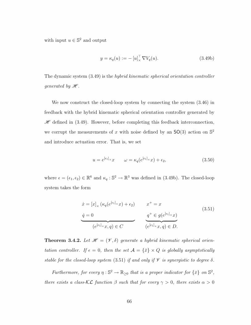
with input u ∈ S2 and output

y = κq(u) := − [u]⊤×∇Vq(u). (3.49b)

The dynamic system (3.49) is the hybrid kinematic spherical orientation controller

generated by H .


feedback with the hybrid kinematic spherical orientation controller generated by

H defined in (3.49). However, before completing this feedback interconnection,

we corrupt the measurements of x with noise defined by an SO(3) action on S2

and introduce actuation error. That is, we set

u = e[ǫ1]×x ω = κq(e

[ǫ1]×x) + ǫ2, (3.50)

where ǫ = (ǫ1, ǫ2) ∈ R6 and κq : S

2 → R3 was defined in (3.49b). The closed-loop

system takes the form

x = [x]× (κq(e[ǫ1]

×x) + ǫ2)

q = 0︸︷︷︸

(e[ǫ1]×x, q) ∈ C

x+ = x

q+ ∈ g(e[ǫ1]×x)

︸︷︷︸(e[ǫ1]

×x, q) ∈ D.

(3.51)

Theorem 3.4.2. Let H = (V , δ) generate a hybrid kinematic spherical orien-

tation controller. If ǫ = 0, then the set A = x × Q is globally asymptotically

stable for the closed-loop system (3.51) if and only if V is synergistic to degree δ.

Furthermore, for every η : S2 → R≥0 that is a proper indicator for x on S

2,

there exists a class-KL function β such that for every γ > 0, there exists α > 0

66

such that for every measurable σ : [0,∞) → αB, any solution (x, q) to (3.51)

satisfies

η(x(t, j)) ≤ β(η(x(0, 0)), t+ j) + γ ∀(t, j) ∈ domx.

Proof. The equivalence of global asymptotic stability of A = e1 × Q and the

family V being synergistic to degree δ follow from Theorem 3.2.6 and Lemma 3.2.7.


Theorem 6.6] and the fact that S2 is compact.

3.4.3 Synergistic Potentials for S2 via Angular Warping

Define the function Φ : S2 → SO(3) as

Φ(x, k, P, u) = R(kP (x), u) = exp(kP (x) [u]×), (3.52)

where k ∈ R, P ∈ C 1x (S2), and u ∈ S

2 are fixed parameters. Then, we define the

transformation T : S2 → S

2 as

T (x, k, P, u) = Φ(x, k, P, u)x, (3.53)

where again, k ∈ R, P ∈ C 1x (S2), and u ∈ S

2 are regarded as fixed parameters

and often dropped from the notation. In context, given a gain, k ∈ R, a potential

function P ∈ C 1x (S2), and a rotation axis u ∈ S

2, T applies a rotation in the

amount of kP (x) to x about the fixed vector u. Note that T (u) = u. This

will have the effect of stretching or compressing the unit sphere, while leaving x

undisturbed.

Theorem 3.4.3. Let k ∈ R, P ∈ C 1x (S2), u ∈ S

2, V ∈ P and define Θ : S2 →

67

R3×3 as

Θ(x) = I − ku∇P (x)⊤ [x]× . (3.54)

Then, the transformation T : S2 → S

2 defined in (3.53) satisfies

T (x) = x (3.55)

DT (x) = Φ(x)(I + k [u]× x∇P (x)⊤

)(3.56)

det DT (x) = 1 + k⟨∇P (x), [u]× x

⟩(3.57)

− [x]⊤×∇(V T )(x) = −Θ(x)⊤Φ(x)⊤ [T (x)]⊤× ∇V (T (x)) (3.58)

T (x) = [T (x)]× Φ(x)Θ(x)ω. (3.59)

Moreover, when det DT (x) 6= 0,

Θ(x)−1 = I +ku∇P (x)⊤ [x]×

det DT (x)(3.60)

CritV T = T −1(CritV ). (3.61)

for all x ∈ S2.


We now state that T is a diffeomorphism of S2, provided that k satisfies a

simple bound.

Theorem 3.4.4. Given k ∈ R, P ∈ C 1x (S2), and u ∈ S

2, if

|k| < 1

max‖∇P (x)‖ : x ∈ S2 . (3.62)

then the transformation T : S2 → S

2 as defined as in (3.53) is a diffeomorphism.

68

Proof. From the Cauchy-Schwarz inequality [129, Ch. 5.1], it follows that

|k⟨∇P (x), [u]× x

⟩| ≤ |k|‖∇P (x)‖2‖ [u]× x‖2.

Then, since ‖ [u]× x‖2 ≤ ‖u‖2‖x‖2 = 1, it follows that when k satisfies (3.62), then

det DT (x) 6= 0 for all x ∈ S2. From the inverse function theorem, this proves that

T is a local diffeomorphism.

Now, since T is continuous, the inverse image of closed sets are closed. Since

the domain of T is S2 and T is 2-norm preserving, it follows that the inverse

image of bounded sets must be bounded. Hence T is a proper mapping, that is,

the inverse image of compact subsets are compact. Since S2 is simply connected,

we apply [130, Theorem B] to conclude that T is a diffeomorphism.

Remark. In Theorem 3.3.4, we showed that an analogous transformation for S1

was a diffeomorphism despite the fact that [130, Theorem B] is not applicable

since S1 is not simply connected.

Given the condition (3.62) for T to be a diffeomorphism, we note that T can

be used to construct new potential functions and control laws for S2. We note

that this result follows from Theorem 3.4.4.

Corollary 3.4.5. Let V ∈ P, let P ∈ C 1x (S2), and let u ∈ S

2. If k ∈ R satisfies

(3.62), then V T ∈ P.

Figures 3.5 and 3.6 show points on S2 and a vector field on S

2, respectively,

before and after the transformation T is applied. Clearly, the critical point of P ∗

(with x = −e3) is moved from e3 to another point.

69

x1x1x2x2

x3

x3 0

00

0

00

1

1

1

1

1

1

−1

−1

−1−1

−1

−1

Figure 3.5. Points on S2 before and after transformation by T , where T is defined

with k = 1/2, P = P ∗, x = −e3, and u = e2.

x1x1x2x2

x3

x3 0

00

0

00

1

1

1

1

1

1

−1

−1

−1−1

−1

−1

Figure 3.6. Gradient descent of potential functions on S2 with respect to −e3.

The plot on the left shows the vectors corresponding to the gradient descent ofP ∗. The plot on the right shows the vectors corresponding to the gradient descentof P ∗ T , where T is defined with P = P ∗, k = 1/2, and u = e2.

70

0 0.5 1−2

−1

0

k

µ(V

k)

Figure 3.7. Plot of µ(V k) for the family of potential functions in Example 3.4.6.A choice of 0 > −δ > µ(V k) provides a synergistic family of potential functionson S

2 with respect to −e3. In fact, this plot is exactly the same as Figure 3.3 inExample 3.3.6.

Example 3.4.6. Define V k1 (x) = P ∗(T (x, k, P ∗, u)), V k

2 (x) = P ∗(T (x,−k, P ∗, u)),

where x = −e3 and u = e2. Then, define the family V k = V k1 , V

k2 . It is not

difficult to compute µ(V k) for every k ∈ [0, 1), for which we provide a plot in

Figure 3.7.

3.4.4 Global Asymptotic Stabilization of the Inverted Equi-

librium Manifold of the 3-D Pendulum

In this section, we illustrate an application of the hybrid feedback control for

spherical orientation in to stabilizing the “inverted equilibrium manifold” of the

so-called “3D pendulum,” first studied in [32]. The state space of the 3D pen-

dulum evolves on the tangent bundle of the compact manifold SO(3), TSO(3),

or equivalently, SO(3) × R3. As pointed out in [2], the complex geometry of this

state space precludes the existence of a smooth state-feedback control law that

globally asymptotically stabilizes a desired configuration on SO(3), or a “reduced

71

x1x2

x3 0

0 0

1

11

−1

−1 −1

Figure 3.8. The overlapping vector fields and regions seen here are generatedfrom the synergistic family V k in Example 3.4.6, with k = ±1/2. The dark (blue)arrows and thick line correspond to the vector field and boundary of the flow setwhen k = 1/2 (q = 1) and δ = 1/4. The analogous lighter (red) arrows and lineare for k = −1/2 (q = 2).

attitude” orientation that evolves on the unit sphere. As pointed out in [126],

smooth feedback control laws can create undesired unstable equilibrium mani-

folds. In contrast, the non-smooth feedback proposed in [127] eliminates these

undesired equilibrium manifolds; however, it is not globally defined and can pro-

duce arbitrarily large control torques. When bounded non-smooth feedback is

used, arbitrarily small measurement noise can destroy the robustness of attrac-

tivity at points where the closed-loop vector field opposes itself over discontinu-

ities [78,131–133].

Dynamics of the 3D Pendulum

In this section, we summarize the dynamical properties of the so-called 3D

pendulum. An in-depth study of the nonlinear dynamics of the 3D pendulum can

72

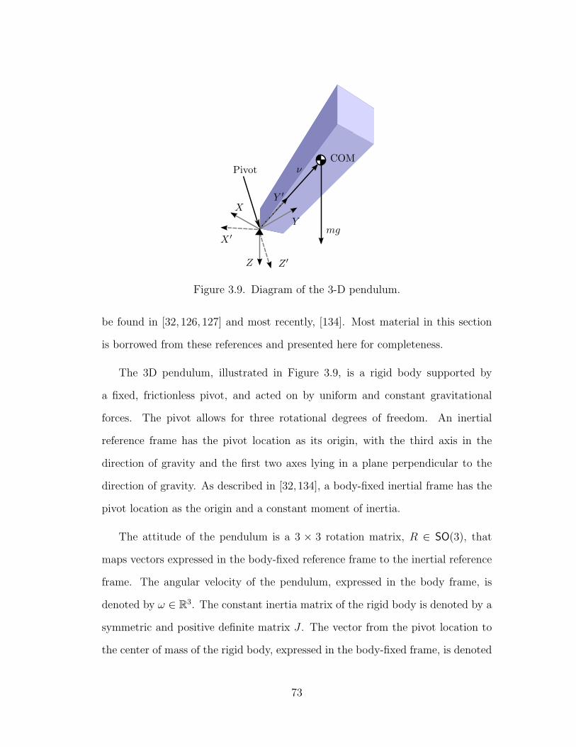
Pivot

X

Y

Z

X ′

Y ′

Z ′

νCOM

mg

Figure 3.9. Diagram of the 3-D pendulum.

be found in [32, 126, 127] and most recently, [134]. Most material in this section

is borrowed from these references and presented here for completeness.

The 3D pendulum, illustrated in Figure 3.9, is a rigid body supported by

a fixed, frictionless pivot, and acted on by uniform and constant gravitational

forces. The pivot allows for three rotational degrees of freedom. An inertial

reference frame has the pivot location as its origin, with the third axis in the

direction of gravity and the first two axes lying in a plane perpendicular to the

direction of gravity. As described in [32,134], a body-fixed inertial frame has the

pivot location as the origin and a constant moment of inertia.

The attitude of the pendulum is a 3 × 3 rotation matrix, R ∈ SO(3), that

maps vectors expressed in the body-fixed reference frame to the inertial reference

frame. The angular velocity of the pendulum, expressed in the body frame, is

denoted by ω ∈ R3. The constant inertia matrix of the rigid body is denoted by a

symmetric and positive definite matrix J . The vector from the pivot location to

the center of mass of the rigid body, expressed in the body-fixed frame, is denoted

73

by ν 6= 0. The symbols g and m denote the constant acceleration due to gravity

and the mass of the pendulum, respectively. Finally τ ∈ R3 is a vector of external

control torques.

The dynamics of the pendulum are given as

R = R [ω]×

Jω = [Jω]× ω +mg [ν]×R⊤e3 + τ

(R,ω) ∈ SO(3) × R

3. (3.63)

It is easy to see that the unforced (τ = 0) pendulum has two equilibrium manifolds

corresponding to attitudes satisfying ω = 0 and

R⊤e3 =ν

‖ν‖ or R⊤e3 = − ν

‖ν‖ , (3.64)

indicating that the gravity vector, expressed in the body-fixed frame, is colinear

with ν, the (body-fixed) vector from the pivot to the center of mass. We define

[R]h =

R ∈ SO(3) : R⊤e3 =

ν

‖ν‖

(3.65)

[R]i =

R ∈ SO(3) : R⊤e3 = − ν

‖ν‖

, (3.66)

which will we call the hanging attitude manifold and the inverted attitude manifold,

respectively. With this notation, we note that the equilibria of (3.63) are contained

in either the hanging equilibrium manifold, [R]h×0, or the inverted equilibrium

manifold, [R]i×0. As pointed out in [32,134], the hanging equilibrium manifold

is stable, and the inverted equilibrium manifold is unstable.

In this paper, we study a reduced-order model, written in terms of the re-

duced attitude vector, Γ = R⊤e3 ∈ S2, which expresses the direction of gravity

74

in the body-fixed frame. This reduction can be written explicitly in terms of the

equivalence relation

[R] =Rs ∈ SO(3) : Rs = RR(R⊤e3, θ), θ ∈ R

. (3.67)

In this direction, for each R ∈ SO(3), we can identify [R] with Γ = R⊤e3 ∈ S2 and

(Γ, ω) evolves on the quotient space TSO(3)/S1, or equivalently, S2×R

3, according

to

Γ = [Γ]× ω

Jω = [Jω]× ω +mg [ν]× Γ + τ

(Γ, ω) ∈ S

2 × R3. (3.68)

The (unforced) equilibria satisfying ω = 0 are (Γi, 0) and (Γh, 0), where

Γh =ν

‖ν‖ and Γi = − ν

‖ν‖ (3.69)

are identified with the hanging and inverted attitude manifolds, respectively. For

a compact exposition, we define

x = (Γ, ω) ∈ S2 × R

3 (3.70)

f(x, τ) =

[Γ]× ω

J−1([Jω]× ω +mg [ν]× Γ + τ)

(3.71)

and shorten (3.68) to

x = f(x, τ) x ∈ S2 × R

3. (3.72)

For the remainder of this paper, we will concern ourselves with stabilizing the

inverted equilibrium, (Γi, 0), of (3.68).

75

Reduced Attitude Control with Synergistic Potentials

In this section, we propose a hybrid feedback that globally asymptotically

stabilizes the inverted equilibrium of (3.68) using synergistic potential functions

on S2 examined previously. Every potential function gives rise to a control law

defined on S2 × R

3 and in particular, for (3.68).

Now, we can introduce our hybrid control structure. Given a family of poten-

tial functions V = Vqq∈Q, we define the sets

C = (Γ, ω, q) : ρ(Γ) − Vq(Γ) ≥ −δ

D = (Γ, ω, q) : ρ(Γ) − Vq(Γ) ≤ −δ,

where ρ(Γ) = minq∈Q Vq(Γ) was defined in (3.20a). Further, we let π and φ denote

the canonical projections from S2×R

3 onto S2 and R

3, respectively. That is, given

(Γ, ω) ∈ S2 × R

3,

π(Γ, ω) = Γ φ(Γ, ω) = ω.

The function g : S2

Q is defined as in (3.20b). Finally, we will make use of

functions that provide “damping injection” for kinetic energy dissipation in the

remainder of this thesis.

Definition 3.4.7. A continuous function Ψ : Rn → R

n is strongly passive if there

exist class K functions α1, α2 such that

α1(‖ω‖) ≤ ω⊤Ψ(ω) ≤ α2(‖ω‖). (3.73)

Definition 3.4.8. Let Q = 1, . . . , N. Given a family of potential functions

V = Vqq∈Q on S2 with respect to Γi, positive numbers δ, c, and a strongly passive

76

function Ψ : R3 → R

3 be strongly passive. Then, the tuple H = (V , δ, c,Ψ) is

said to generate the dynamic system

q = 0 (u, q) ∈ C

q+ ∈ g(π(u)) (u, q) ∈ D

(3.74a)

with input u ∈ S2 × R

3 and output

y = κq(u) = −mg [ν]× π(u) − c [π(u)]⊤× ∇Vq(π(u)) − Ψ(φ(u)). (3.74b)

The dynamic system (3.74) is the hybrid 3D pendulum stabilizer generated by H .

We now construct the closed-loop system by connecting the system (3.72)

in feedback with the hybrid 3D pendulum stabilizer generated by H defined in

(3.74). However, before completing this feedback interconnection, we corrupt the

measurements of Γ and ω with noise and introduce actuation error. That is, we

set

u = (e[ǫ1]×Γ, ω + ǫ2) τ = κq(e

[ǫ1]×Γ, ω + ǫ2) + ǫ3, (3.75)

where ǫ = (ǫ1, ǫ2, ǫ3) ∈ R9 and κq : S

2 × R3 → R

3 was defined in (3.74b). This

yields the closed-loop system

Γ = [Γ]× ω

Jω = [Jω]× ω +mg [ν]× Γ + κq(e[ǫ1]

×Γ, ω + ǫ2) + ǫ3

q = 0︸︷︷︸

(e[ǫ1]×Γ, ω + ǫ2, q) ∈ C

Γ+ = Γ

ω+ = ω

q+ = g(e[ǫ1]×Γ)

︸︷︷︸(e[ǫ1]

×Γ, ω + ǫ2, q) ∈ D(3.76)

Theorem 3.4.9. Let H = (V , δ, c,Ψ) generate a hybrid 3D pendulum stabilizer.

77

If ǫ = 0, then the set A = (Γi, 0) × Q is globally asymptotically stable for the

closed-loop system (3.76) if and only if V is synergistic with gap exceeding δ.

Furthermore, for every η : S2×R

3 → R≥0 that is a proper indicator for (Γi, 0)

on S2 × R

3, there exists a class-KL function β such that for every compact set

K ⊂ R3 and every γ > 0, there exists α > 0 such that for every measurable

ǫ : [0,∞) → αB, any solution ξ = (Γ, ω, q) to (3.76) with ω(0, 0) ∈ K, satisfies

η(ξ(t, j)) ≤ β(η(ξ(0, 0)), t+ j) + γ ∀(t, j) ∈ dom ξ.


Remark. The work [126] proposes the smooth feedback

κs(Γ, ω) = K(Γ) [Γi]× Γ − Ψ(ω), (3.77)

where K(Γ) = Φ′ (12P ∗(Γ)

)+ σ (and P ∗ was defined in (3.48) with x = Γi),

Φ : R≥0 → R≥0 is a nondecreasing twice continuously differentiable function

satisfying Φ(0) = 0, Φ′ denotes the derivative of Φ, and σ is chosen to satisfy

σ > mg|ν|. We note that (3.77) could be written as

κs(Γ, ω) = − [Γ]⊤×∇A(Γ) −mg [ν]× Γ − Ψ(ω),

where A(Γ) = 2Φ(

12P ∗(Γ)

)+ σP ∗(Γ) and σ = σ −mg|ν|.

The benefit of the smooth feedback (3.77) is that it requires slightly less in-

formation than simply canceling the gravitational torque. In particular, (3.77)

requires only knowledge of Γi = −ν/|ν| and an upper bound on mg|ν|, rather

than complete knowledge of mgν.

78

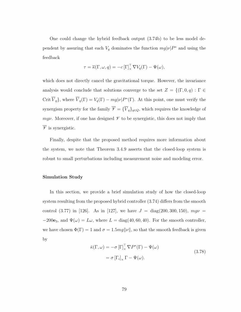
One could change the hybrid feedback output (3.74b) to be less model de-

pendent by assuring that each Vq dominates the function mg|ν|P ∗ and using the

feedback

τ = κ(Γ, ω, q) = −c [Γ]⊤×∇Vq(Γ) − Ψ(ω),

which does not directly cancel the gravitational torque. However, the invariance

analysis would conclude that solutions converge to the set Z = (Γ, 0, q) : Γ ∈

CritV q, where V q(Γ) = Vq(Γ) −mg|ν|P ∗(Γ). At this point, one must verify the

synergism property for the family V = V qq∈Q, which requires the knowledge of

mgν. Moreover, if one has designed V to be synergistic, this does not imply that

V is synergistic.

Finally, despite that the proposed method requires more information about

the system, we note that Theorem 3.4.9 asserts that the closed-loop system is

robust to small perturbations including measurement noise and modeling error.

Simulation Study

In this section, we provide a brief simulation study of how the closed-loop

system resulting from the proposed hybrid controller (3.74) differs from the smooth

control (3.77) in [126]. As in [127], we have J = diag(200, 300, 150), mgν =

−200e3, and Ψ(ω) = Lω, where L = diag(40, 60, 40). For the smooth controller,

we have chosen Φ(Γ) = 1 and σ = 1.5mg‖ν‖, so that the smooth feedback is given

by

κ(Γ, ω) = −σ [Γ]⊤× ∇P ∗(Γ) − Ψ(ω)

= σ [Γi]× Γ − Ψ(ω).

(3.78)

79

The parameters specific to the hybrid 3D pendulum stabilizer are the same as in

Example 3.4.6, with k = 0.25, δ = 0.15 and c = 0.5mg|ν|. The output of the

hybrid controller is given as

κq(Γ, ω) = −mg [ν]× Γ − 0.5mg|ν| [Γ]⊤× ∇Vq(Γ) − Ψ(ω).

The initial condition of the pendulum system is Γ(0) = [0 h√

1 − h2]⊤, ω(0) =

5e3, with h = 0.001. The hybrid controller begins with q = 1 (k = 0.25).

In both cases, the evolution of Γ ∈ S2 is pictured in Figure 3.10 and measures

of error signals and control effort are pictured in Figure 3.11. In particular, the

error measure

θ(Γ) = cos−1(Γ⊤i Γ)

gives the angle between Γ and Γi. Figure 3.11 illustrates an important difference

between the hybrid feedback and the smooth feedback. As described in [126,

127], any smooth feedback control law is subject to performance limitations. In

particular, as Γ approaches a critical point of P ∗ (referring to (3.77)), the feedback

term resulting from the potential function vanishes. This creates an unstable

equilibrium point where ω = 0 and Γ = −Γi = Γh. Trajectories starting arbitrarily

close to this equilibrium may take arbitrarily long to diverge from it.

In contrast, the hybrid 3D pendulum stabilizer is not subject to such perfor-

mance limitations. This is due to the fact that the flow and jump sets are built

so that if Γ is approaching a “bad” critical point of Vq, q will switch to some

value p ∈ Q, so that another controller can be used, where Γ is not close to a

“bad” critical point of Vp. This effectively eliminates the possibility of the feed-

back term from the potential function disappearing. Finally, Figure 3.12 shows

80

−1

0

1−1

0

1

−1

0

1

Hybrid

Smooth

Γ1

Γ2

Γ3

Figure 3.10. Trajectories of Γ for smooth and hybrid controllers. Hybrid controlis depicted in blue, smooth in red.

signals related to the hybrid controller. In particular, the values of V1 and V2 are

plotted on the same plot, with the value of Vq highlighted by a thick dashed line.

Figure 3.12 also shows the signals ρ(Γ)−Vq(Γ) and q. When ρ(Γ)−Vq(Γ) reaches

−δ, a switch is made in q.

To give a more exaggerated view of the hybrid controller and to show how

changing the value of k can change performance, we conduct another simulation.

The following simulation is mostly the same as the previous simulation, with the

following important changes: k = 0.75, δ = 0.5, and K = diag(8, 12, 8) (exactly

1/5 of the previous gain). Changing the value of k has the important consequence

that the critical points of Vq will be moved further from the hanging equilibrium

and increasing δ will make the controller more reluctant to switch. Decreasing K

by 4/5 will underdamp the response, allowing the 3D pendulum to rotate quite

wildly, driving Γ into regions where different controllers apply. Figures 3.13, 3.14,

81

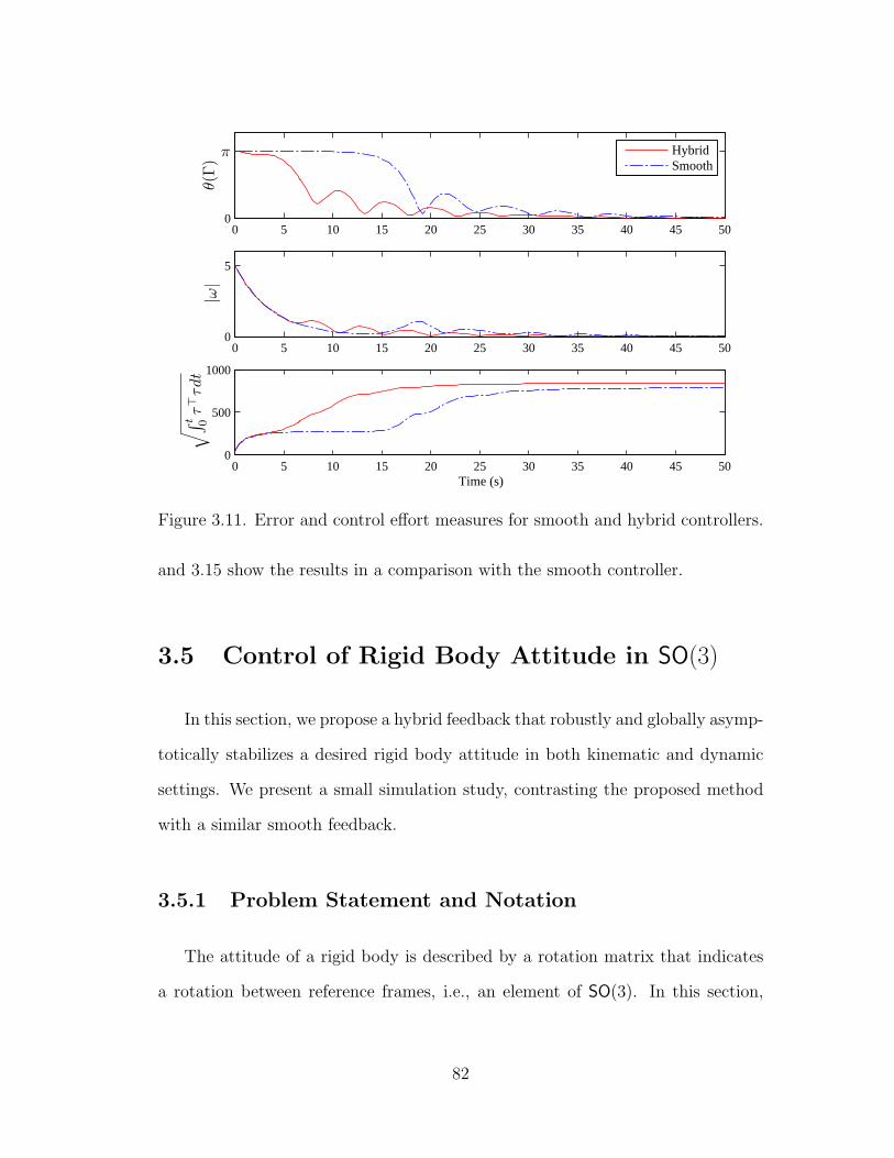
0 5 10 15 20 25 30 35 40 45 500

HybridSmooth

0 5 10 15 20 25 30 35 40 45 500

5

0 5 10 15 20 25 30 35 40 45 500

500

1000

Time (s)

θ(Γ)

|ω|

√∫ t 0

τ⊤τdt

π

Figure 3.11. Error and control effort measures for smooth and hybrid controllers.

and 3.15 show the results in a comparison with the smooth controller.

3.5 Control of Rigid Body Attitude in SO(3)

In this section, we propose a hybrid feedback that robustly and globally asymp-

totically stabilizes a desired rigid body attitude in both kinematic and dynamic

settings. We present a small simulation study, contrasting the proposed method

with a similar smooth feedback.


The attitude of a rigid body is described by a rotation matrix that indicates

a rotation between reference frames, i.e., an element of SO(3). In this section,

82

0 5 10 15 200

1

2

0 5 10 15 20

0

0 5 10 15 201

2

Time (s)

−δρ(Γ

)−

Vq(Γ

)V

1(Γ

),V

2(Γ

)q

Figure 3.12. Signals related to hybrid controller for the 3D pendulum. Thetop plot shows the values of the two potential functions used to determine theswitching condition - the current potential function being used is highlighted.The middle plot shows the signal ρ(Γ) − Vq(Γ) - when it reaches δ, a controlswitch is initiated. The bottom plot shows the value of q.

83

−1

0

1−1

0

1

−1

0

1

Hybrid

Smooth

Γ1

Γ2

Γ3

Figure 3.13. Trajectories of Γ for smooth and hybrid controllers. Hybrid controlis depicted in blue, smooth in red.

0 50 100 1500

HybridSmooth

0 50 100 1500

5

0 50 100 1500

1000

2000

Time (s)

θ(Γ)

|ω|

√∫ t 0

τ⊤τdt

π

Figure 3.14. Error and control effort measures for smooth and hybrid controllers.

84

0 5 10 15 200

1

2

0 5 10 15 20

0

0 5 10 15 20

1

2

Time (s)

−δρ(Γ

)−

Vq(Γ

)V

1(Γ

),V

2(Γ

)q

Figure 3.15. Signals related to hybrid controller for the 3D pendulum. Thetop plot shows the values of the two potential functions used to determine theswitching condition - the current potential function being used is highlighted.The middle plot shows the signal ρ(Γ) − Vq(Γ) - when it reaches δ, a controlswitch is initiated. The bottom plot shows the value of q.

85

the matrix R will denote the attitude of a rigid body, where R rotates vectors

expressed in the local body frame coordinates to their inertial frame coordinates.

We denote the angular velocity of the rigid body, given in body frame coordinates,

as ω, J = J⊤ > 0 denotes the inertia matrix of the rigid body, and τ is a vector

of external torques at our disposal. Then, given a measurable ω : R → R3, the

rigid body satisfies the kinematic and dynamic equations

R = R [ω]× (3.79a)

Jω = [Jω]× ω + τ. (3.79b)

We refer the reader to Appendix E for useful properties of the cross product used

here.

Rigid body attitude is often parametrized in terms of a rotation θ ∈ R about

a fixed axis u ∈ S2 by the so-called Rodrigues formula (3.45)–the map R(θ, u) :

R × S2 → SO(3) defined as

R(θ, u) = I + sin θ [u]× + (1 − cos θ) [u]2× .

This matrix has eigenvalues 1, ejθ, e−jθ, where the 1-dimensional subspace de-

fined by the axis u ∈ S2 is unchanged by R, that is, R(θ, u)u = R(θ, u)⊤u = u.

We recall the fact, shown in Appendix E, that R(θ, u) = eθ[u]× . Given an element

of SO(3), it is fairly simple to recover the angle and axis of rotation using

u sin θ = ψ (R(θ, u)) 2(1 − cos θ) = trace(I −R(θ, u)), (3.80)

86

where ψ : R3×3 → R

3 is defined as

ψ(A) = vec× (skewA) =1

2

A32 − A23

A13 − A31

A21 − A12

.

Many useful properties of ψ are shown in Appendix E. Finally, it is worth noting

that R(θ, u) is 2-π periodic in θ and that

R(θ,−u) = R(−θ, u). (3.81)

Analogous to S1 and S

2, given a potential function on SO(3), the form of

(3.79a) allows us to characterize the set of critical points succinctly. In particular,

given a function V : SO(3) → R, we can compute its change along flows of the

kinematic equation (3.79a) as

dV (R(t))

dt=⟨∇V (R), R [ω]×

⟩

= 2ω⊤ψ(R⊤∇V (R))

(3.82)

where we have used the property (E.5c). So, no matter the value of ω, when

ψ(∇V (R)⊤R) = 0 (if and only if ∇V (R)⊤R is symmetric), there is no infinitesimal

change in V . In this direction, we define the set of critical points of some V :

SO(3) → R as

CritV = R ∈ SO(3) : ψ(R⊤∇V (R)) = 0. (3.83)

As mentioned in Section 3.3.1, the point stabilization problem on S1 can easily

be reduced to the stabilization of an identity element. This is a general property

87

of Lie groups (see e.g. [11]), which applies to SO(3) as well. So, without loss of

generality, we will first consider constructing a velocity feedback (using ω, the

angular velocity as a control variable) to stabilize I for the kinematic subsystem,

which evolves on SO(3). This velocity feedback will then be naturally extended

into dynamics evolving on TSO(3) (equivalently, SO(3) × R3) by using kinetic

energy as a Lyapunov function [13] for stabilization of (I, 0) ∈ SO(3) × R3.

Perhaps, the most natural potential function on SO(3) with respect to I is the

“height” function on SO(3),

P ∗(R) = trace(I −R). (3.84)

We will investigate the critical points of this function later in this section.

3.5.2 Hybrid Control Structure: Kinematics & Dynamics

The kinematic equation of motion on SO(3) provide an explicit form for the

gradient of a potential function in terms of the angular velocity ω. In this section,

we state specialized versions of Theorem 3.2.6 with accompanying statements

regarding the robustness to measurement noise of the closed-loop system.

Kinematic stabilization to I ∈ SO(3)

Analogously to our hybrid controllers proposed for S1 and S

2, the functions ρ

and g and the sets C and D do not change from (3.20) and nor does the dynamic

equation of the logic state q in (3.21a). The only change is to the output y, which

becomes y = −2ψ(R⊤∇Vq(R)). The controller and closed-loop system subjected

88

to measurement noise are given as follows.

Definition 3.5.1. Given V = Vqq∈Q, a family of potential functions on SO(3)

with respect to I ∈ SO(3) and δ > 0, the pair H = (V , δ) is said to generate the

dynamic system

q = 0 (u, q) ∈ C

q+ ∈ g(u) (u, q) ∈ D

(3.85a)

with input u ∈ SO(3) and output

y = κq(u) := −2ψ(R⊤∇Vq(R)). (3.85b)

The dynamic system (3.85) is the hybrid kinematic attitude controller generated

by H .

We now construct the closed-loop system by connecting the system (3.79a) in

feedback with the hybrid kinematic attitude controller generated by H defined

in (3.85). However, before completing this feedback interconnection, we corrupt

the measurements of R with noise and introduce actuation error. That is, we set

u = e[ǫ1]×R ω = κq(e

[ǫ1]×R) + ǫ2, (3.86)

where ǫ = (ǫ1, ǫ2) ∈ R6 and κq : SO(3) → R

3 was defined in (3.85b). This yields

the closed-loop system

R = R[κq(e

[ǫ1]×R) + ǫ2

]×

q = 0︸︷︷︸

(e[ǫ1]×R, q) ∈ C

R+ = R

q+ ∈ g(e[ǫ1]×R)

︸︷︷︸(e[ǫ1]

×R, q) ∈ D

(3.87)

89

Theorem 3.5.2. Let H = (V , δ) generate a hybrid kinematic attitude controller.

If ǫ = 0, then the set A = I×Q is globally asymptotically stable for the closed-

loop system (3.87) if and only if V is synergistic with gap exceeding δ.

Furthermore, for every η : SO(3) → R≥0 that is a proper indicator for I on

SO(3), there exists a class-KL function β such that for every γ > 0, there exists

α > 0 such that for every measurable ǫ : [0,∞) → αB, any solution (R, q) to

(3.87) satisfies

η(R(t, j)) ≤ β(η(R(0, 0)), t+ j) + γ ∀(t, j) ∈ domR.

Proof. The equivalence of global asymptotic stability of A = I × Q and the

family V being synergistic to degree δ follow from Theorem 3.2.6 and Lemma 3.2.7.


Theorem 6.6] and the fact that SO(3) is compact.

Dynamic stabilization to (I, 0) ∈ SO(3) × R3

To construct the hybrid controller for dynamic stabilization to (I, 0) ∈ SO(3)×

R3, we employ the techniques used in Section 3.4.4 to extend the hybrid kinematic

spherical orientation controller defined on S2 to the 3D pendulum which evolves

on S2 × R

3. Again, we make use of a strongly passive function Ψ, as defined in

Definition 3.4.7 for energy damping. The hybrid control structure is as follows.

Given a family of potential functions V = Vqq∈Q, we define the sets

C = (R,ω, q) : ρ(R) − Vq(R) ≥ −δ

D = (R,ω, q) : ρ(R) − Vq(R) ≤ −δ,

90

where ρ(R) = minq∈Q Vq(R) was defined in (3.20a). Further, we let π and φ denote

the canonical projections from SO(3) × R3 onto SO(3) and R

3 respectively. That

is, given (R,ω) ∈ SO(3) × R3,

π(R,ω) = R φ(R,ω) = ω.

The function g : SO(3) Q is defined in (3.20b).

Definition 3.5.3. Given V = Vqq∈Q, a family of potential functions on SO(3)

with respect to I ∈ SO(3), δ > 0, and a persistent function Ψ, the tuple H =

(V , δ,Ψ) is said to generate the dynamic system

q = 0 (u, q) ∈ C

q+ ∈ g(π(u)) (u, q) ∈ D

(3.88a)

with input u ∈ SO(3) × R3 and output

y = κq(u) := −2ψ(π(u)⊤∇Vq(π(u))) − Ψ(φ(u)). (3.88b)

The dynamic system (3.88) is the hybrid attitude controller generated by H .


feedback with the hybrid attitude controller generated by H defined in (3.88).

However, before completing this feedback interconnection, we corrupt the mea-

surements of (R,ω) with noise and introduce actuation error. That is, we set

u = (e[ǫ1]×R,ω + ǫ2) τ = κq(e

[ǫ1]×R,ω + ǫ2) + ǫ3, (3.89)

where ǫ = (ǫ1, ǫ2, ǫ3) ∈ R9 and κq : SO(3)×R

3 → R3 was defined in (3.88b). This

91

yields the closed-loop system

R = R [ω]×

Jω = [Jω]× ω + κq(e[ǫ1]

×R,ω + ǫ2) + ǫ3

q = 0︸︷︷︸

(e[ǫ1]×R,ω + ǫ2, q) ∈ C

R+ = R

ω+ = ω

q+ ∈ g(e[σ]×R)

︸︷︷︸(e[ǫ1]

×R,ω + ǫ2, q) ∈ D

(3.90)

Theorem 3.5.4. Let H = (V , δ,Ψ) generate a hybrid attitude controller. If

ǫ = 0, then the set A = (I, 0) × Q is globally asymptotically stable for the

closed-loop system (3.90) if and only if V is synergistic with gap exceeding δ.

Furthermore, for every η : SO(3) × R3 → R≥0 that is a proper indicator for

(I, 0) on SO(3) × R3, there exists a class-KL function β such that for every

γ > 0 and every compact set K ⊂ R3, there exists α > 0 such that for every

measurable ǫ : [0,∞) → αB, any solution (R,ω, q) to (3.90) with ω(0, 0) ∈ K

satisfies

η((R(t, j), ω(t, j)) ≤ β(η(R(0, 0), ω(0, 0)), t+ j) + γ ∀(t, j) ∈ dom ξ.


Remark. The hybrid controller proposed here can also stabilize a specified inverted

equilibrium of the 3D pendulum described in Section 3.4.4 by directly cancelling

the torque due to gravity.

92

3.5.3 Not-So-Synergistic Potential Functions on SO(3)

Before resorting to diffeomorphisms of SO(3) to construct synergistic families

of potential functions, we consider the possibility that a large class of existing

potential functions on SO(3) might already be large enough to find a synergistic

family. This large class of potential functions on SO(3) stems from what is known

as the “modified trace function.” Recall that the “height” function on SO(3) was

defined in (3.84) as P ∗(R) = trace(I −R). It is instructive to see that

P ∗(R) = trace(I −R) =1

2〈I −R, I −R〉 =

1

2trace((I −R)⊤(I −R)).

That is, P ∗ is simply the restriction of the Frobenius norm of the error between R

and I to SO(3). The same is also true of the height functions on Sn investigated

previously.

A generalization of P ∗ can be found by using the inner product 〈X,Y 〉A =

〈X,AY 〉, where A is a symmetric and positive definite matrix. Thus, we define

the modified trace function,

PA(R) = trace(A(I −R)) =1

2〈I −R,A(I −R)〉 , (3.91)

which, taking inspiration from [110], was first introduced in [13]. It is also helpful

to see PA in the angle-axis representation through (3.45). Given θ ∈ R and u ∈ S2,

PA(R(θ, u)) = (1 − cos θ)(trace(A) − u⊤Au). (3.92)

93

Clearly, we also have that

P ∗(R(θ, u)) = 2(1 − cos θ). (3.93)

As we now show, the critical points of PA are the identity element and rotations

of 180 about the (real) eigenvectors of A. In this direction, for some A ∈ Rn×n,

we define

E (A) = (λ, v) ∈ C × Cn : Av = λv, |v| = 1 (3.94)

and its projections onto C and Cn as

Eλ(A) = λ ∈ C : ∃(λ, v) ∈ E (A) (3.95)

Ev(A) = v ∈ Cn : ∃(λ, v) ∈ E (A). (3.96)

Recall that when A is symmetric, Eλ(A) ⊂ R. In this case, it is helpful to constrain

the sets of unit eigenvectors to be purely real as well. In this direction, we let

E R

v (A) = v ∈ Rn : ∃(λ, v) ∈ E (A). (3.97)

Lemma 3.5.5. Let A ∈ R3×3 be symmetric and positive definite. Then, the

function PA satisfies

CritPA = I ∪ R(π,E R

v (A)). (3.98)

When A has distinct eigenvalues, PA is a perfect Morse function.


Lemma 3.5.5 agrees with the existing analysis in [110,111,126], which showed

94

that in the special case when A = ∆ := diag(d1, d2, d3), with d1 > d2 > d3 > 0,

CritP∆ =I,(

1 0 00 −1 00 0 −1

),( −1 0 0

0 1 00 0 −1

),( −1 0 0

0 −1 00 0 1

),

which corresponds to the identity element of SO(3) and rotations of 180 about

each principal axis of the body frame coordinate system. As shown in Lemma

3.5.5, when A has distinct eigenvalues, PA is a perfect Morse function and attains

the minimal number of critical points on SO(3) possible [110]. These desirable

properties make it a popular candidate for control and observer design [11,13,79,

81–83,135,136].

As pointed out in [13, 137], when A does not have distinct eigenvalues, parts

of the critical set become connected. In the case when A has only 1 distinct

eigenvalue (A = αI, α ∈ R), we have PαI = αP ∗. It is obvious in this case that

CritP ∗ = R ∈ SO(3) : R = R⊤, (3.99)

and as a result of Lemma 3.5.5, we can characterize this set as

CritP ∗ = I ∪ R(π,S2) :

the union of the identity element and the connected submanifold of 180 rotations

about any axis. Note that

Υ := CritP ∗ \ I = R ∈ SO(3) : R = R⊤ 6= I = R(π,S2) (3.100)

is not diffeomorphic to S2. Since R(π, u) = R(−π,−u) = R(π,−u), the antipo-

dal points of S2 are identified through the Rodrigues formula. Hence, Υ is an

95

embedding of the real projective plane, RP 2, in SO(3) [13].

To a lesser extent (than A with distinct eigenvalues), this particular choice of

function is also a popular choice for Lyapunov analysis and control design [84,138–

140]. It is interesting to observe that any symmetric positive definite matrix with

identical eigenvalues is arbitrarily close to a symmetric positive definite matrix

with distinct eigenvalues (for instance, I is close to I + ǫ diag(1, 2, 3)), so one can

see that a slight perturbation of P ∗ can cause the set of critical points to change

quite dramatically. This is not too surprising, as the set of Morse functions is

known to be an open dense set in the space of differentiable functions [105].

Since one can use (3.91) to produce any number of potential functions on

SO(3) with respect to I, having only I as a common critical point, one might

wonder whether one can find a synergistic family of potential functions of the

form V = PAqq∈Q. Indeed, it would seem possible on the surface, especially

since it is easy to separate the critical sets between functions by choosing different

A’s with different eigenvectors; however, the following lemmas show that this is

not the case.

Theorem 3.5.6. Let N ∈ 1, 2, . . . . If AqNq=1 satisfies Aq = A⊤q > 0 for

every q ∈ 1, . . . , N, then, the family V = VqNq=1 ∈ PN , where Vq(R) =

trace(Aq(I −R)), is not synergistic.


Perhaps, Theorem 3.5.6 seems, on the surface, a bit counter-intuitive. Cer-

tainly, if one selects two positive definite matrices with distinct eigenvalues and

distinct eigenvectors, their only common critical point is the identity matrix.

Unfortunately, this is not a sufficient condition for synergism. The following

96

lemma sheds some light as to why this is the case. Recall that for any function

V : SO(3) → R, that V (R) = 2ω⊤ψ(R⊤∇V (R)). Then, to flow down the gradient

of V , one can set ω = −2ψ(R⊤∇V (R)).

Lemma 3.5.7. Let A ∈ R3×3 be symmetric and positive definite. Suppose the

kinematic feedback ω = −2ψ(R⊤∇PA(R)) = 2ψ(R⊤A) is applied to the system

R = R [ω]×. Then, Υ is invariant for the closed-loop system

R = R [κPA(R)]× = R

[2 vec× skewR⊤A

]× = R−RAR.

Proof. Suppose that R = R⊤. Then, R⊤ = (R−RAR)⊤ = R−RAR = R. Since

R is symmetric when R is symmetric, the set of symmetric rotations, I × Υ is

invariant to the flow R = R−RAR. Note that I and Υ are disjoint and in fact,

there exists an open neighborhood U ∋ I such that U ∩Υ = ∅. This implies that

Υ is invariant.

In view of Lemma 3.5.7, the lower number of critical points attained by PA

when A has distinct eigenvalues does little to improve the attractivity properties

of I in a kinematic setting, since any choice of A (distinct eigenvalues or not)

leaves Υ invariant. At least in this case, requiring PA to be a Morse function does

little more than to facilitate statements about the Lebesgue measure or density of

sets from which I is not attractive as in [13,18] and others. The velocity feedback

applied in Lemma 3.5.7 is used in [11,13,79,81–84,136,138–140] as either a velocity

feedback or part of a torque feedback.

Unfortunately, Lemma 3.5.7 effectively rules out the prospect of combining

multiple potential functions of the form PA and their corresponding control laws

in a hybrid scheme that achieves global asymptotic stability of I, since any con-

97

trol law generated by this class renders Υ invariant. Further, it seems that a

set of suitable potential functions and their corresponding control laws is hard to

come by. To the best of the author’s knowledge, there does not appear to be any

use of potential functions on SO(3) in the literature other than P ∗ and PA (or

strictly increasing real functions of these) in the literature. In this direction, we

will again create a large class of potential functions based on an angular stretch-

ing/compression of SO(3), analogous to the transformations considered for S1 and

S2.

3.5.4 Synergistic Potentials for SO(3) via Angular Warping

In order to create a new class of potential functions on SO(3), we “warp” SO(3)

by a transformation, then apply a known potential function to the warped space.

In this direction, we define T : SO(3) → SO(3) as

T (R, k, P, u) = exp(kP (R) [u]×)R, (3.101)

where k ∈ R, P ∈ C 1I (SO(3)), and u ∈ S

2. In context, given R ∈ SO(3), the

transformation T applies an additional rotation to R about a fixed axis u ∈

S2. The amount of rotation about u is controlled by the function P and a gain

k. While T depends on arguments other than R, we will regard these as fixed

“parameters” of a given transformation and often drop these arguments when

there is no confusion. This transformation has several useful properties.

Theorem 3.5.8. Let k ∈ R, P ∈ C 1I (SO(3)), u ∈ S

2, V ∈ P, and define

98

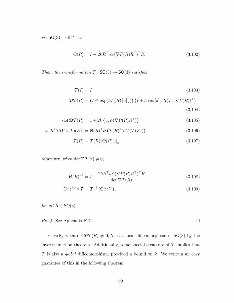
Θ : SO(3) → R3×3 as

Θ(R) = I + 2kR⊤uψ(∇P (R)R⊤)⊤R. (3.102)

Then, the transformation T : SO(3) → SO(3) satisfies

T (I) = I (3.103)

DT (R) =(I ⊗ exp(kP (R) [u]×)

) (I + k vec [u]×R(vec∇P (R))⊤

)

(3.104)

det DT (R) = 1 + 2k⟨u, ψ(∇P (R)R⊤)

⟩(3.105)

ψ(R⊤∇(V T )(R)) = Θ(R)⊤ψ(T (R)⊤∇V (T (R))

)(3.106)

T (R) = T (R) [Θ(R)ω]× . (3.107)

Moreover, when det DT (x) 6= 0,

Θ(R)−1 = I − 2kR⊤uψ(∇P (R)R⊤)⊤R

det DT (R)(3.108)

CritV T = T −1 (CritV ) . (3.109)

for all R ∈ SO(3).


Clearly, when det DT (R) 6= 0, T is a local diffeomorphism of SO(3) by the

inverse function theorem. Additionally, some special structure of T implies that

T is also a global diffeomorphism, provided a bound on k. We contain an easy

guarantee of this in the following theorem.

99

Theorem 3.5.9. Given k ∈ R, P ∈ C 1I (SO(3)), u ∈ S

2, if

|k| <√

2

2 maxR∈SO(3)

‖∇P (R)‖F, (3.110)

then the transformation T (R) : SO(3) → SO(3) defined in (3.101) is a diffeomor-

phism.


A simple consequence of Theorem 3.5.8 that when V is a potential function,

so is V T .

Corollary 3.5.10. Let V ∈ P, let P ∈ C 1I (SO(3)), and let u ∈ S

2. If k satisfies

(3.110) then, V T ∈ P.

Now, we see that applying the diffeomorphism T to an existing potential func-

tion produces a new potential function, with new critical points that are calculated

by applying the inverse of T to the critical points of the original potential function,

as shown by (3.109) of Theorem 3.5.8. Of course, this is not all that is necessary

to produce a synergistic family of potential functions, as shown in Theorem 3.5.6.

We now provide an existence result in the form of an example, showing that

it is possible to generate a synergistic family of potential functions using the

transformation T and a particular potential function of the type PA, defined in

(3.91).

Example 3.5.11. Let w = [11 12 13]⊤, ∆ = 3 diag(w)/∑3

i=1wi, u = w/‖w‖2.

Then, define V k1 (R) = P∆(T (R, k, u, P∆)), V k

2 (R) = P∆(T (R,−k, u, P∆)). Then,

100

0 0.1 0.2 0.3 0.4

-1

-0.5

0

k

µ(V

k)

Figure 3.16. Plot of µ(V k) for the family of potential functions in Example 3.5.11.

define the family V k = V k1 , V

k2 , where k satisfies (3.110), or

|k| <√

2/(2 maxR∈SO(3)

‖∆‖F ) ≈ 0.4073.

It is not difficult to compute µ(V k) for every k satisfying this bound, for which

we provide a plot in Figure 3.16.

Remark. The fact that there exists a synergistic family of only 2 potential functions

on SO(3) is remarkable. Recall that the basin of attraction of an asymptotically

stable equilibrium point is contractible. Moreover, the Lusternik-Schnirelmann

category of SO(3) is 4, meaning the minimum number of contractible sets needed

to cover SO(3) is 4. This implies that the union of the basins of attraction of

the identity element for each controller in this synergistic family does not cover

SO(3). Nevertheless, the hybrid scheme still provides global asymptotic stability.

3.5.5 Simulation Results

In this section, we present a simulation study comparing the hybrid controller

with a similar smooth controller. Here, the hybrid controller is generated by the

101

potential functions in Example 3.5.11 and we compare it to a similar smooth

control algorithm resulting from using only one potential function.

In the following simulations (as in Example 3.5.11), we let w = [11 12 13]⊤,

∆ = 3 diag(w)/∑3

i=1wi, J = diag(200, 300, 150), and K = diag(40, 60, 40). The

smooth control law is given as

τs(R,ω) = −2ψ(∆R) −Kω. (3.111)

As in Example 3.5.11, we let u = w/‖w‖2 and set k1 = −k2 = 0.2 and δ = 0.5.

The hybrid control law is given (3.88b), where, for q ∈ 1, 2,

τq(R,ω) = −2Θq(R)⊤ψ(∆Tq(R)) −Kω (3.112)

is used as the torque feedback for mode q and

Tq(R) = exp(kqP∆(R) [u]×)R

Θq(R) = I + 2kqR⊤uψ(−∆R⊤)⊤R

= I + 2kqR⊤uψ(R∆)⊤R.

As a final notational convenience for this section, we let

Vq(R) = P∆(Tq(R)),

for q ∈ 1, 2.

Note that the smooth control law is derived from the potential function P∆(R) =

trace(∆(I−R)) and for each q ∈ 1, 2, the torque feedback from the hybrid con-

troller is derived from the potential function P∆ T (·, kq, P∆, u) = Vq. In some

102

sense, the smooth control law τs (3.111) is the midpoint (in a homotopy sense) of

the two control laws (3.112) used by the hybrid controller.

In the sequel, we define the function θ : SO(3) → R as

θ(R) = cos−1

(1 − 1

2trace(I −R)

)

The simulation in Figures 3.17 and 3.18 compare the hybrid and smooth con-

trollers beginning from an initial condition close to a critical point of P∆ (note

that since ∆ is diagonal, the critical points are 180 rotations about the unit vec-

tors). In particular, the initial value of R was chosen as R(0) = R(π, z), where

z = [√

(1 − h2) h 0]⊤ and h = 0.1. The initial condition of ω was chosen as

zero. For the hybrid controller, the initial condition of q was set to one.

In this simulation, the hybrid controller begins from an initial condition that

is not a critical point for any of its control laws and in fact, forces the rigid body

to converge to the identity rotation without switching q. So, the result of this

simulation merely compares the convergence properties of two smooth control

laws when starting on or near critical points or sufficiently far away from them.

Figures 3.19 and 3.20 depict a similar simulation as Figures 3.17 and 3.18;

however, the initial condition in Figures 3.19 and 3.20 is chosen close to a critical

point of P∆ T1. In particular, the initial value of R was chosen as R(0) =

T−11 (R(π, e1)). The initial condition of ω was chosen as zero. For the hybrid

controller, the initial condition of q was set to one.

In this simulation, the hybrid controller begins from an initial condition that

is a critical point for its initial choice of potential function/control law. Because

δ was selected appropriately (i.e., 0 > −δ > µ(V k), the hybrid controller imme-

103

−10

1 −10

1

−1

0

1

−10

1 −10

1

−1

0

1

x1x1

x2x2

x3

x3

Figure 3.17. Comparison of rigid body trajectories for smooth and hybrid con-trollers starting near a critical point of P∆ with zero initial angular velocity. Thehybrid controller (left) immediately exerts a torque to steer the rigid body around.The smooth controller (right) has close to zero torque near the critical points. Thiscreates a long delay in convergence to the identity rotation. The red trajectory isR(t)e1, the blue is R(t)e2, and the green is R(t)e3.

diately switches q from 1 to 2 (though, not pictured). This results in asymptotic

stability of the identity element and a similar performance to the smooth control

law. For the remainder of this simulation, q remained constant at 2.

Finally, Figures 3.21, 3.22, and 3.23 depict a simulation of the hybrid controller

beginning from the identity rotation, but with an initial angular velocity. In

particular, R(0) = I, ω(0) = 2w/‖w‖2, and q(0) = 1. A comparison with a

smooth controller is not provided as the performance difference is negligible.

In these simulations, the initial spin causes the rigid body to rotate through

180 and near critical points of the potential functions used by the hybrid con-

troller. When R(t) approaches these critical points, the hybrid controller detects

it by a difference between its potential functions and switches the control law

accordingly.

Figure 3.23 details the logic behavior of the hybrid controller over the simu-

104

0 100 200 300 400 500 600 700 800 900 10000

Hybrid

Smooth

0 100 200 300 400 500 600 700 800 900 10000

0.02

0.04

0.06

0 100 200 300 400 500 600 700 800 900 10000

1

2

Time (s)

π

θ(R

)‖ω

‖ 2√∫ t 0

τ⊤

τdt

Figure 3.18. Comparison of smooth and hybrid controllers starting near a criticalpoint of P∆ with zero initial angular velocity. The hybrid controller (solid, blue)immediately exerts a torque to steer the rigid body around. The smooth controller(dashed, red) has close to zero torque near the critical points. This creates a longdelay in convergence to the identity rotation.

105

−10

1 −10

1

−1

0

1

−10

1 −10

1

−1

0

1

x1x1

x2x2

x3

x3

Figure 3.19. Comparison of rigid body trajectories for smooth and hybrid con-trollers starting near a critical point of P∆ T1 with zero initial angular velocity.The hybrid controller (left) immediately switches two a new control law and ex-hibits similar performance to the smooth controller (right). The red trajectory isR(t)e1, the blue is R(t)e2, and the green is R(t)e3.

lation. This figure displays the values of Vq(R(t)) (thin solid and dashed lines)

and indicates the current value of q by a bold dashed line line. Additionally, the

signals ρ(R) − Vq(R) and q are shown as well. When t = 0, R(t) = I, and both

potential functions have the same value of zero. When the angular velocity rotates

the rigid body, the potential functions diverge in value and the hybrid controller

switches the value of q to match the index of the lowest-valued potential function.

106

0 20 40 60 80 100 120 140 160 1800

HybridSmooth

0 20 40 60 80 100 120 140 160 1800

0.02

0.04

0.06

0 20 40 60 80 100 120 140 160 1800

1

2

3

Time (s)

π

θ(R

)‖ω

‖ 2√∫ t 0

τ⊤

τdt

Figure 3.20. Comparison of smooth and hybrid controllers starting near a criticalpoint of P∆ with zero initial angular velocity. The hybrid controller (solid, blue)immediately exerts a torque to steer the rigid body around. The smooth controller(dashed, red) has close to zero torque near the critical points. This creates a longdelay in convergence to the identity rotation.

107

−1

0

1

−1

0

1

−1

0

1

x1x2

x3

Figure 3.21. Rigid body trajectory for hybrid controller starting from R(0) = Iand ω(0) = 2w/‖w‖2. The hybrid controller damps the oscillations and switchesbetween control laws as the initial angular velocity moves the rigid body nearcritical points of the hybrid controller’s family of potential functions. The redtrajectory is R(t)e1, the blue is R(t)e2, and the green is R(t)e3.

108

0 50 100 1500

0 50 100 1500

1

2

0 50 100 1500

2

4x 10

4

Time (s)

π

θ(R

)‖ω

‖ 2√∫ t 0

τ⊤

τdt

Figure 3.22. Rigid body trajectory characteristics and control effort for hybridcontroller starting from R(0) = I and ω(0) = 2w/‖w‖2.

109

0 5 10 15 200

2

4

0 5 10 15 20

0

0 5 10 15 201

2

Time (s)

−δρ(R

)−

Vq(R

)V

1(R

),V

2(R

)q

Figure 3.23. Plot of hybrid controller’s potential functions and its selection ofcontrol laws. As the rigid body is rotated near critical points, the control law isswitched to the index of the minimum-valued potential function.

110

Chapter 4

Quaternion-Based Attitude

Control

The attitude of a rigid body is, by definition, an element of SO(3); however, it is

possible to represent SO(3) using various coordinate systems. Often, the set of unit

quaternions, sometimes referred to as Euler parameters, are used to parametrize

SO(3). This parametrization provides a globally nonsingular representation of

rigid body attitude and uses the minimal number of parameters (four) needed to

represent SO(3) without singularity [85]. However, the unit quaternions present

a problematic ambiguity, as there are exactly two unit quaternions representing

each element of SO(3).

Recall again that the attitude of a rigid body can be parametrized as a rotation

about a fixed axis by the Rodrigues formula (3.45)–the map R(θ, u) : R × S2 →

SO(3)–defined as

R(θ, u) = I + sin θ [u]× + (1 − cos θ) [u]2× .

111

In the sense of (3.45), a unit quaternion, q, is defined as

q =

η

ǫ

= ±

cos(θ/2)

sin(θ/2)u

∈ S

3, (4.1)

where η ∈ R is referred to as the “scalar” component and ǫ ∈ R3 is referred to as

the “vector” component. In this way, a unit quaternion represents an element of

SO(3) through the map R : S3 → SO(3) defined as

R(q) = I + 2η [ǫ]× + 2 [ǫ]2× . (4.2)

Note the important property that R(q) = R(−q) for each q ∈ S3. Also note that

we have abused notation by “overloading” the symbol R; however, the domain of

the operator it represents will always be determined by its argument. We denote

the set-valued inverse map Q : SO(3) S3 as

Q(R) = q ∈ S3 : R(q) = R. (4.3)

For convenience in notation, we will often write a quaternion as q = (η, ǫ), rather

than in the form of a vector.

With the identity element i = (1, 0) ∈ S3, each unit quaternion q ∈ S

3 has an

inverse q−1 = (η,−ǫ) under the quaternion multiplication rule

q1 ⊙ q2 =

η1η2 − ǫ⊤1 ǫ2

η1ǫ2 + η2ǫ1 + [ǫ1]× ǫ2

,

where qi = (ηi, ǫi) ∈ R4 and i ∈ 1, 2. This multiplication rule is a group

112

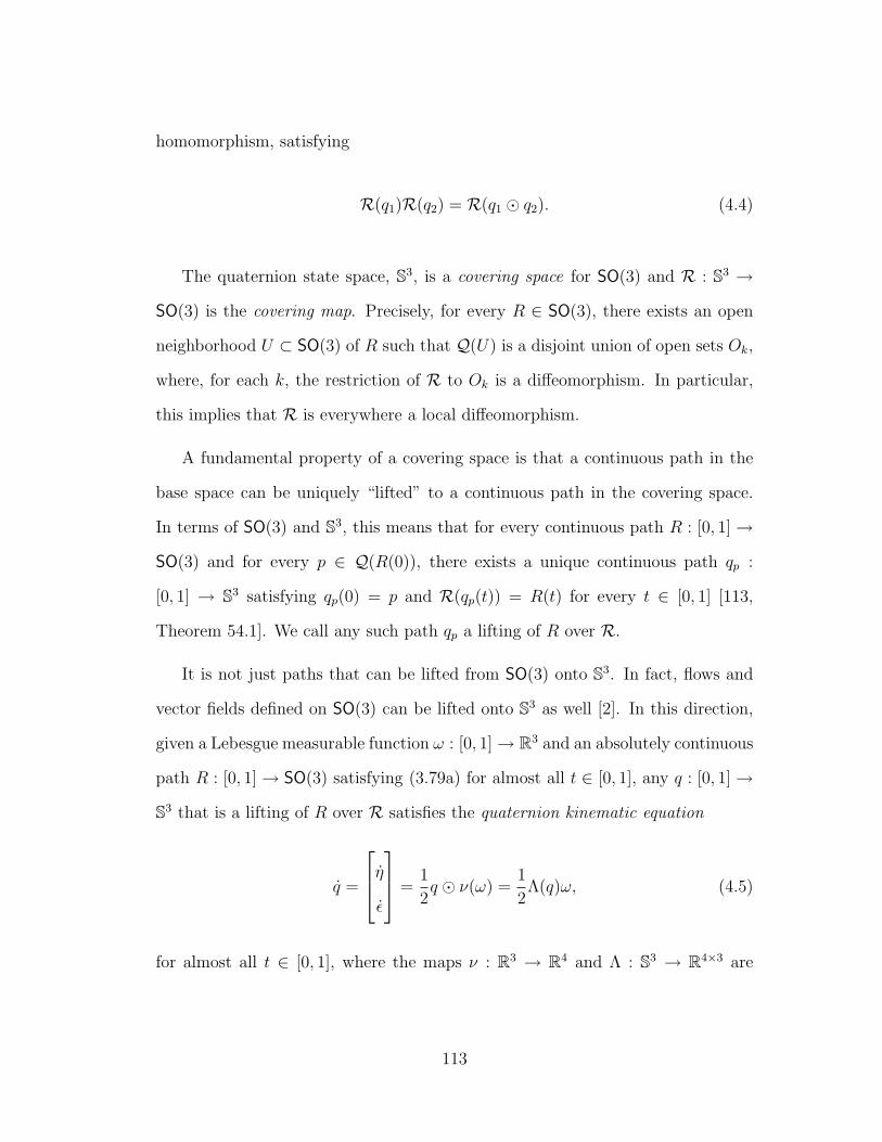
homomorphism, satisfying

R(q1)R(q2) = R(q1 ⊙ q2). (4.4)

The quaternion state space, S3, is a covering space for SO(3) and R : S

3 →

SO(3) is the covering map. Precisely, for every R ∈ SO(3), there exists an open

neighborhood U ⊂ SO(3) of R such that Q(U) is a disjoint union of open sets Ok,

where, for each k, the restriction of R to Ok is a diffeomorphism. In particular,

this implies that R is everywhere a local diffeomorphism.

A fundamental property of a covering space is that a continuous path in the

base space can be uniquely “lifted” to a continuous path in the covering space.

In terms of SO(3) and S3, this means that for every continuous path R : [0, 1] →

SO(3) and for every p ∈ Q(R(0)), there exists a unique continuous path qp :

[0, 1] → S3 satisfying qp(0) = p and R(qp(t)) = R(t) for every t ∈ [0, 1] [113,

Theorem 54.1]. We call any such path qp a lifting of R over R.

It is not just paths that can be lifted from SO(3) onto S3. In fact, flows and

vector fields defined on SO(3) can be lifted onto S3 as well [2]. In this direction,

given a Lebesgue measurable function ω : [0, 1] → R3 and an absolutely continuous

path R : [0, 1] → SO(3) satisfying (3.79a) for almost all t ∈ [0, 1], any q : [0, 1] →

S3 that is a lifting of R over R satisfies the quaternion kinematic equation

q =

η

ǫ

=

1

2q ⊙ ν(ω) =

1

2Λ(q)ω, (4.5)

for almost all t ∈ [0, 1], where the maps ν : R3 → R

4 and Λ : S3 → R

4×3 are

113

defined as

ν(x) =

0

x

(4.6)

Λ(p) =

−ǫ⊤

ηI + [ǫ]×

. (4.7)

For a wealth of information about quaternions, we refer the reader to [115, 141–

143].

As we study in the next section, the act of using a quaternion-based feedback

that works on paths lifted from SO(3) to S3 changes the topological structure of

the control objective. As a point stabilization problem in SO(3), the objective is

the stabilize a single equilibrium point. When translated into an equivalent point

stabilization problem in S3, the objective changes to stabilizing a disconnected set

of two antipodal points on S3.

4.1 Disambiguation

A feedback controller designed using a quaternion representation of attitude

may not be consistent with a control law defined on SO(3). That is, for every rigid

body attitude, the quaternion-based feedback controller may be ambiguous and

take on one of two possible values; hence, they may not be well-defined on SO(3).

When this is the case, analysis for quaternion-based feedback is often carried out

in S3 using the lifted attitude kinematic equation (4.5), but these results are not

directly related to a feedback system that takes measurements from SO(3). This

obviously begs the following questions: How is a unit quaternion obtained from

114

a measurement of attitude? On what state-space is an inconsistent quaternion-

based feedback defined? How is stability analysis done in the covering space

related to a stability result for the actual, physical system? As we will see, these

questions are deeply connected to the operation of lifting a continuous path in

SO(3) to S3.

While calculating the set of two quaternions that represent a given attitude is

a fairly simple operation (see e.g. [115, 144–148]), the process of selecting which

quaternion to use for feedback is a less obvious operation. As noted in [28], it

is often the case that the quaternion with positive “scalar” component is used

for feedback. This operation is non-global (the scalar component could easily be

zero) and discontinuous. As we show in this work, when such a discontinuous

quaternion selection scheme is paired with a widely-used inconsistent quaternion-

based feedback, the resulting closed-loop system is not robust to arbitrarily small

measurement noise. In fact, we construct an explicit noise signal defined on SO(3)

that stabilizes a region about the manifold of 180 rotations with zero angular

velocity when such a feedback is employed.

Here, we present a simple hybrid dynamic algorithm for lifting a path from

SO(3) to S3. That is, given a continuous trajectory in SO(3), the lifting system dy-

namically produces a continuous quaternion trajectory. Our approach here allows

us to make a clear equivalence between stability results for a closed-loop system in

the covering space and stability results for an inherently dynamic feedback control

system for the actual plant. This justifies carrying out stability analysis on the

covering space; however, when a quaternion-based feedback does not respect the

two-to-one covering of SO(3), this translated stability result may not actually be

desirable!

115

When the proposed hybrid path-lifting system is paired with an inconsistent

quaternion-based feedback, the noise sensitivity issues disappear; however, it can

introduce the so-called “unwinding phenomenon,” where the feedback can un-

necessarily rotate the rigid body up to a full rotation due to ambiguities in the

quaternion representation of attitude. This behavior was discussed at length in [2]

in terms of lifts of paths and vector fields from SO(3) to S3. The results here allow

for a characterization of unwinding in terms of the projection of asymptotically

stable sets in an extended state space onto the plant state space.

4.1.1 Inconsistent Quaternion-based Control Laws and Path

Lifting

It is quite commonplace in the attitude control literature to design a feedback

based upon a quaternion representation of rigid body attitude. That is, the control

designer creates a continuous function κ : S3 × R

3 → R3 and closes a feedback

loop around (3.79) by setting τ(t) = κ(q(t), ω(t)), where q(t) is selected to satisfy

R(q(t)) = R(t), for each t ∈ R≥0. When the feedback κ satisfies

κ(q, ω) = κ(−q, ω) ∀q ∈ S3, (4.8)

we say that κ is consistent. Equivalently, for every R ∈ SO(3) and every ω ∈ R3,

κ(Q(R), ω) is single-valued and the feedback τ = κ(Q(R), ω) leads to a uniquely-

defined vector field on SO(3) × R3. Smooth and consistent feedback control al-

gorithms are investigated in [87] for adaptive attitude control without angular

velocity measurements and recently in [149] for attitude synchronization of a for-

mation of spacecraft where (in addition to other terms) −ηǫ is used for feedback.

116

Interestingly, this can be written as the negative gradient feedback for the poten-

tial function 14trace(I − R(q)) = 1 − η2. In such cases, there is little need for a

quaternion representation, as κ might as well be defined in terms of R ∈ SO(3),

rather than its quaternion representation.

When a quaternion-based feedback is inconsistent, that is,

∃q ∈ S3 κ(q, ω) 6= κ(−q, ω), (4.9)

the resulting feedback does not define a unique vector field on SO(3)×R3 because

for some R ∈ SO(3) the feedback κ(Q(R), ω) is multi-valued [2]. At this point, the

control designer must, for every t ∈ R≥0, choose which q(t) ∈ Q(R(t)) to use for

feedback. Or, in the topological terms of lifting, the control designer must choose

how to lift the measured attitude trajectory in SO(3) to S3. In this direction, we

provide a quote from the seminal paper [28]:

“In many quaternion extraction algorithms, the sign of [the ‘scalar’part of the quaternion] is arbitrarily chosen positive. This approachis not used here, instead, the sign ambiguity is resolved by choosingthe one that satisfies the associated kinematic differential equation. Inimplementation, this would probably imply keeping some immediatepast values of the quaternion.”

There is much insight to be gained from this quotation, especially when

viewed in the context of lifts under R. In particular, it suggests that incon-

sistent quaternion-based control laws require an extra quaternion memory state

to lift the measured SO(3) trajectory to S3. In this direction, we reconstruct

the discontinuous quaternion “extraction” algorithm mentioned in the quotation

above in terms of a metric and use the ensuing discussion to motivate a hybrid

algorithm for on-line lifting of a measured attitude trajectory from SO(3) to S3.

117

Let P : S3 → [0, 2] be defined as

P (q) = P (η, ǫ) = 1 − i⊤q = 1 − η. (4.10)

Note that since q ∈ S3, P satisfies the identity

P (q) =1

2(q − i)⊤(q − i) =

1

2(q⊤q − 2q⊤i + i⊤i) = 1 − i⊤q. (4.11)

Then, the function d : S3 × S

3 → [0, 2] defined as

d(q, p) = P (q−1 ⊙ p) = 1 − q⊤p (4.12)

defines a metric on S3. From a geometric viewpoint, d(q, p) is the height of p on

S3 “above” the plane perpendicular to the vector q at q. Given a set Q ⊂ S

3, we

define the distance to Q from q (in terms of the metric d) as

dist(q,Q) = infd(q, p) : p ∈ Q. (4.13)

When the set Q in (4.13) takes the form of Q(R) for some R ∈ SO(3), the distance

function also takes a special form. In particular, let Q(R) = p,−p. Then,

dist(q,Q(R)) = mind(q, p), d(q,−p) = 1 − |q⊤p|. (4.14)

One candidate method to lift a path from SO(3) to S3 is to simply pick the

quaternion representation of R that is closest to a specific quaternion in terms of

118

the metric d. In particular, let us define the map Φ : S3 × SO(3) S

3 as

Φ(q, R) = argminp∈Q(R)

d(q, p) = argmaxp∈Q(R)

q⊤p. (4.15)

The map Φ has some useful properties, which we summarize in the following

lemmas.

Lemma 4.1.1. Let q ∈ S3 and R ∈ SO(3). The following are equivalent.

1. Φ(q, R) is single-valued.

2. 0 ≤ dist(q,Q(R)) < 1.

3. q⊤p 6= 0 for all p ∈ Q(R) so that q⊤Φ(q, R) > 0.

4. R 6= R(π, u)R(q) for some u ∈ S2.

Proof. Throughout this proof, we let Q(R) = p,−p. By the definition of Φ in

(4.15), we see that Φ(q, R) is single-valued if and only if d(q, p) 6= d(q,−p) ⇔

1 − q⊤p 6= 1 + q⊤p ⇔ q⊤p 6= −q⊤p ⇔ q⊤p 6= 0 ⇔ 0 ≤ dist(q,Q(R)) < 1. This

provides an equivalence between 1), 2), and 3), above.

Now, let θ ∈ R and u ∈ S2 be such that R = R(θ, u)R(q). Since R =

R(±p), the fact that R satisfies (4.4) provides the following equivalent series of

expressions:

R(p) = R(θ, u)R(q)

R(p)R(q)−1 = R(θ, u)

R(p⊙ q−1) = R(θ, u).

Now, since p⊙ q−1 = (p⊤q, ∗) (i.e. the η component of p⊙ q−1 is p⊤q), the form

of R : S3 → SO(3) in (4.2) guarantees that R(p ⊙ q−1) = R(p ⊙ q−1)⊤ 6= I if

119

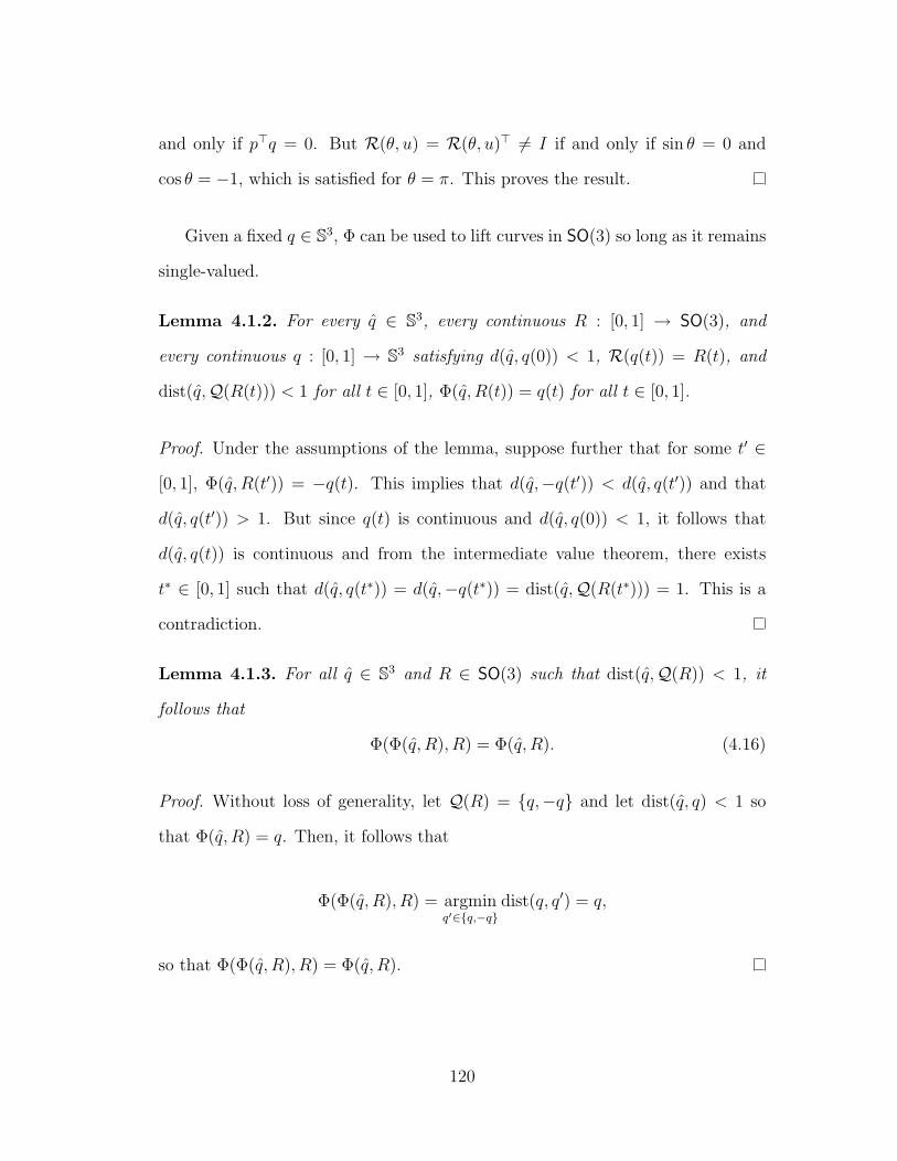
and only if p⊤q = 0. But R(θ, u) = R(θ, u)⊤ 6= I if and only if sin θ = 0 and

cos θ = −1, which is satisfied for θ = π. This proves the result.

Given a fixed q ∈ S3, Φ can be used to lift curves in SO(3) so long as it remains

single-valued.

Lemma 4.1.2. For every q ∈ S3, every continuous R : [0, 1] → SO(3), and

every continuous q : [0, 1] → S3 satisfying d(q, q(0)) < 1, R(q(t)) = R(t), and

dist(q,Q(R(t))) < 1 for all t ∈ [0, 1], Φ(q, R(t)) = q(t) for all t ∈ [0, 1].

Proof. Under the assumptions of the lemma, suppose further that for some t′ ∈

[0, 1], Φ(q, R(t′)) = −q(t). This implies that d(q,−q(t′)) < d(q, q(t′)) and that

d(q, q(t′)) > 1. But since q(t) is continuous and d(q, q(0)) < 1, it follows that

d(q, q(t)) is continuous and from the intermediate value theorem, there exists

t∗ ∈ [0, 1] such that d(q, q(t∗)) = d(q,−q(t∗)) = dist(q,Q(R(t∗))) = 1. This is a

contradiction.

Lemma 4.1.3. For all q ∈ S3 and R ∈ SO(3) such that dist(q,Q(R)) < 1, it

follows that

Φ(Φ(q, R), R) = Φ(q, R). (4.16)

Proof. Without loss of generality, let Q(R) = q,−q and let dist(q, q) < 1 so

that Φ(q, R) = q. Then, it follows that

Φ(Φ(q, R), R) = argminq′∈q,−q

dist(q, q′) = q,

so that Φ(Φ(q, R), R) = Φ(q, R).

120

Since a goal of attitude control is to regulate R to I, one might choose i as a

point of reference (since R(i) = I) and use the map Φi : SO(3) S3 defined as

Φi(R) = Φ(i, R). (4.17)

Now, following 3) from Lemma 4.1.1 we see that i⊤Φi(R) > 0, that is, Φi always

chooses the quaternion with positive scalar component, so long as it is single-

valued. Further, Lemma 4.1.2 allows one to lift curves with Φi so long as R does

not cross the manifold of 180 rotations, where Φi is multi-valued, or else Φi will

produce a quaternion trajectory that is discontinuous. This can have disastrous

effects when Φi is composed with an inconsistent feedback. We now examine such

a feedback.

Let c > 0 and let Ψ : R3 → R

3 be strongly passive (see Definition 3.4.7). Now,

consider the inconsistent feedback

κ∗(q, ω) = −cǫ− Ψ(ω) = −cΛ(q)⊤i − Ψ(ω). (4.18)

In (4.18), the cǫ term introduces a rotational spring force and L(ω) introduces

damping. While this control law asymptotically stabilizes (i, 0) for the lifted

closed-loop system defined by (4.5), (3.79b), and setting τ = κ∗(q, ω), it renders

(−i, 0) an unstable equilibrium point. We now show that when composed with

Φi, the result is not robust to arbitrarily small measurement noise. In particular,

we show that a malicious noise signal can stabilize the 180 manifold.

121

Define the signum function sgn : R → −1, 0, 1 as

sgn(s) =

1 s > 0

0 s = 0

−1 s < 0.

(4.19)

Then, for 0 ≤ δ < π, consider the (discontinuous) function ∆ : SO(3) × R3 →

R(δ,S2) defined as

∆(R(θ, u), ω) =

R(−δ sgn(ω⊤u), u) cos θ < cos(π + δ)

I otherwise.

(4.20)

Note that for any (R,ω) ∈ SO(3)×R3, the rotation matrix ∆(R,ω)R constitutes

an angular perturbation of R in the amount of δ and as δ decreases to zero, ∆

converges to the identity matrix. We note that (4.20) is well defined on SO(3).

Lemma 4.1.4. For every δ ∈ [0, π) and (R,ω) ∈ SO(3)×R3, ∆(R,ω) is uniquely

defined.

Proof. Suppose that R = R(θ, u) for some θ ∈ R and u ∈ S2. Clearly, ∆(R,ω) is

uniquely defined when either ω = 0 or cos θ = cos(θ + 2πZ) ≥ cos(π ± δ), since it

doesn’t depend on either R or ω in this case.

Now, suppose that cos θ < cos(π ± δ) and ω 6= 0. This implies that R 6= I,

since 0 < δ < π. Then, by Euler’s theorem on rotations, for any v ∈ S2 and φ

such that R = R(φ, v), it must be the case that u = v or u = −v (only when

122

R 6= I). Now, since R(−θ,−u) = R(θ, u), it follows that

∆(R(φ, v), ω) = R(−δ sgn(ω⊤v), v) = R(−δ sgn(ω⊤u), u).

So, we have shown that the value of ∆ is independent of the angle and axis

representation used for R, hence, it is uniquely defined on SO(3) × R3.

Let φi : SO(3) → S3 be any single-valued selection of Φi, that is, φi(R) = Φi(R)

for all R 6= R(π, u) and φi(R) ∈ Φi otherwise. Now, we apply the noise signal ∆ to

measurements of attitude before being converted to a quaternion for use with the

inconsistent feedback (4.18) and analyze the resulting closed-loop system. That

is, we replace q with φi(∆(R,ω)R) in the control law κ∗ defined in (4.18).

Because φi and ∆ are discontinuous, we use the notion of Krasovskii solutions

for discontinuous systems [4].

Definition 4.1.5. Let f : Rn → R

n. The Krasovskii regularization of f is the

set-valued mapping

K f(x) =⋂

ǫ>0

convf(x+ ǫB) (4.21)

where convB denotes the closed convex hull of the set B ⊂ Rn and B denotes the

unit ball in Rn. Then, given a function f : R

n → Rn, a Krasovskii solution to

x = f(x) on an interval I ⊂ R≥0 is an absolutely continuous function satisfying

x(t) ∈ K f(x(t)) (4.22)

for almost all t ∈ I.

An important property of a Krasovskii regularization is that K f(x) = f(x)

123

for every x where the function f is continuous.

Theorem 4.1.6. Let a > 0, c > 0, and δ > 0 satisfy

0 < δ <1

2

(−ac

+

√(ac

)2

+ 8

)<

√2 (4.23)

and define

B = (R(θ, u), ω) : cos θ + (1/a)ω⊤Jω ≤ cos(π + δ).

Then, the set R(π,S2) × 0 is stable and B is invariant for the Krasovskii

regularization of the closed-loop system

R = R [ω]×

Jω = [Jω]× ω − cΛ(φi(∆(R,ω)R))⊤i − L(ω).

(4.24)


This result shows that the discontinuity created by pairing an inconsistent

quaternion-based feedback with a discontinuous quaternion selection scheme is

susceptible to arbitrarily small measurement noise. This is because at the discon-

tinuity of Φi (on the manifold R(π,S2)), the feedback term cΛ(Φi(R))⊤i opposes

itself about the discontinuity. Then, malicious noise signals, like (4.20) can ex-

ploit the discontinuity of the vector field to induce a chattering behavior that

stabilizes R(π,S2) × 0. This is quite similar to the inconsistent feedback

κd(q, ω) = − sgn(η)ǫ− ω (when implemented with a lifted trajectory), which was

shown in [131] to exhibit extreme noise sensitivity that can destroy global attrac-

tivity properties of a desired attitude in a kinematic setting.

124

Unfortunately, the various failures of Φi have led several authors (e.g. [150])

to derive sufficient conditions on the initial conditions of (3.79) to ensure that

these 180 attitudes are never approached, thus obviating the use of a globally

nonsingular representation of attitude like unit quaternions. However, the issues

with using Φi as a path-lifting algorithm are not a problem with the quaternion

representation–they arise because Φi is a static (i.e. memoryless) map from SO(3)

to S3, which cannot be continuous because SO(3) and S

3 are not homeomorphic.

In particular, Φi always chooses the closest quaternion to i. In general, when one

compares Q(R) with q for some R ∈ SO(3) and q ∈ S3, there is a 2-D manifold

p ∈ S3 : p⊤q where Φ(q, R) is multi-valued. However, when the reference point

for choosing the closest quaternion is allowed to change, it is then possible to create

a dynamic algorithm for lifting a trajectory in SO(3) to S3. We now explore such

an algorithm that is hybrid in nature.

4.1.2 A Hybrid Algorithm for Dynamic Path Lifting

In this section, we present a simple dynamic algorithm for lifting a path from

SO(3) to S3. The main feature of the algorithm is a memory state q ∈ S

3 that

provides a reference point for choosing the closest quaternion with respect to d.

This memory state usually remains constant, but is updated only when necessary

to ensure that dist(q,Q(R)) < 1. The basic logic behind the algorithm is pictured

in a flow chart in Fig. 4.1.

Given a number 0 < α < 1, we define the sets Cℓ, Dℓ ⊂ SO(3) × S3 as

Cℓ = (q, R) ∈ SO(3) × S3 : dist(q,Q(R)) ≤ α

Dℓ = (q, R) ∈ SO(3) × S3 : dist(q,Q(R)) ≥ α.

(4.25a)

125

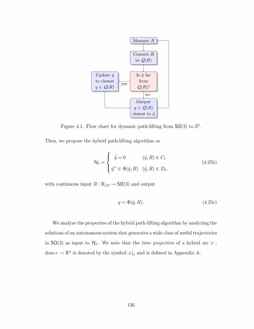
Measure R

Convert R

to Q(R)

Is q far

from

Q(R)?

Output

q ∈ Q(R)

closest to q

Update q

to closest

q ∈ Q(R)

no

yes

Figure 4.1. Flow chart for dynamic path-lifting from SO(3) to S3.

Then, we propose the hybrid path-lifting algorithm as

Hℓ =

˙q = 0 (q, R) ∈ Cℓ

q+ ∈ Φ(q, R) (q, R) ∈ Dℓ,

(4.25b)

with continuous input R : R≥0 → SO(3) and output

q = Φ(q, R). (4.25c)

We analyze the properties of the hybrid path-lifting algorithm by analyzing the

solutions of an autonomous system that generates a wide class of useful trajectories

in SO(3) as input to Hℓ. We note that the time projection of a hybrid arc x :

domx→ Rn is denoted by the symbol x↓t and is defined in Appendix A.

126

Theorem 4.1.7. Let α ∈ (0, 1). The hybrid system

˙q = 0

R ∈ R [MB]×︸︷︷︸(q, R) ∈ Cℓ

q+ ∈ Φ(q, R)

R+ = R︸︷︷︸(q, R) ∈ Dℓ

(4.26a)

and its output

q = Φ(q, R) (4.26b)

have the following properties:

1. All maximal solutions are complete.

2. The time between jumps is bounded below by 2α/M .

3. The function q↓t : R≥0 → S3 is continuous and satisfies R(q↓t (t)) =

R↓t (t).


From Theorem 4.1.7 and its proof, one could also append dynamical equations

for the output q(t, j) = Φ(q(t, j), R(t, j)) to (4.26a) as q ∈ 12q⊗ν(MB) and q+ = q

(note that one should actually write ω ∈MB, q = 12q ⊗ ν(ω), and R = R [ω]×, so

that q and R are acted on by the same angular velocity).

With a hybrid algorithm for path lifting in place, we consider the feedback in-

terconnection of (3.79) with the hybrid path-lifting system and a quaternion-based

hybrid controller. Consider the hybrid controller Hc, that takes a measurement

127

y ∈ S3 × R

3 as input, has a state ξ ∈ X ⊂ Rn, has dynamics

Hc

ξ ∈ Fc(y, ξ) (y, ξ) ∈ Cc

ξ+ ∈ Gc(y, ξ) (y, ξ) ∈ Dc,

(4.27)

and produces a continuous torque output κ : S3 ×R

3 ×X → R3. We assume that

Hc satisfies the hybrid basic conditions as well.

Often, quaternion-based controllers are analyzed using the lifted attitude dy-

namics, defined by equations (4.5) and (3.79b), thus neglecting any auxiliary

lifting system. The next theorem essentially justifies this approach by relating so-

lutions of the whole closed-loop system (including the hybrid path-lifting system)

to a reduced system that has the quaternion-based hybrid controller in feedback

with the lifted system defined by (4.5) and (3.79b).

Before stating the theorem, we define two closed-loop systems. The first

closed-loop system is the feedback interconnection of (3.79) with the series in-

terconnection of Hℓ and Hc. This yields the system H1 with state (R,ω, q, ξ) ∈

SO(3) × R3 × S

3 ×X defined as

R = R [ω]×

Jω = [Jω]× ω + κ(Φ(q, R), ω, ξ)

˙q = 0

ξ ∈ Fc(Φ(q, R), ω, ξ)︸︷︷︸(q, R) ∈ Cℓ, (Φ(q, R), ω, ξ) ∈ Cc

R+ = R

ω+ = ω

q+ ∈ Φ(q, R)

ξ+ = ξ︸︷︷︸(q, R) ∈ Dℓ,

R+ = R

ω+ = ω

q+ = q

ξ+ ∈ Gc(Φ(q, R), ω, ξ)︸︷︷︸(Φ(q, R), ω, ξ) ∈ Dc.

(4.28)

In (4.28), we mean that flows can only occur when flows can occur for both

the controller and lifting subsystems. Jumps can occur when either the con-

128

troller or lifting subsystems can jump. It may be possible that both (q, R) ∈ Dℓ

and (Φ(q, R), ω, ξ) ∈ Dc are satisfied at the same “time,” i.e. Dℓ ∩ Dc 6= ∅,

in which case, either jump is possible. That is, either q+ ∈ Φ(q, R) or ξ+ ∈

Gc(Φ(q, R), ω, ξ) (the other states do not change). This is necessary to ensure

that the closed-loop system satisfies the hybrid basic conditions.

Now, we define the feedback interconnection of the lifted attitude system and

the hybrid controller Hc. This yields the reduced system H2 with state (q, ω, ξ) ∈

S3 × R

3 ×X defined as

q =1

2q ⊗ ν(ω)

Jω = [Jω]× ω + κ(q, ω, ξ)

ξ ∈ Fc(q, ω, ξ)︸︷︷︸

(q, ω, ξ) ∈ Cc

q+ = q

ω+ = ω

ξ+ ∈ Gc(q, ω, ξ)︸︷︷︸(q, ω, ξ) ∈ Dc.

(4.29)

For the coming theorem, we adopt the economical notation

(x1(t, j), . . . , xk(t, j)) = (x1, . . . , xk)|(t,j).

Lemma 4.1.8. For every solution (R1, ω1, q1, ξ1) : E1 → SO(3)× R3 × S

3 ×X to

(4.28) such that dist(q1,Q(R1))|(0,0) < 1, there exists a solution (q2, ω2, ξ2) : E2 →

S3 ×R

3 ×X to (4.29) such that for every (t, j) ∈ E1, there exists j′ ≤ j such that

(t, j′) ∈ E2 and

(R1,Φ(q1, R1), ω1, ξ1)|(t,j) = (R(q2), q2, ω2, ξ2)|(t,j′). (4.30)

Conversely, for every solution (q2, ω2, ξ2) : E2 → S3 × R

3 ×X to (4.29), there

129

exists a solution (R1, ω1, q1, ξ1) : E1 → SO(3) × R3 × S

3 × X to (4.28) such that

dist(q1,Q(R1))|(0,0) < 1 and for every (t, j′) ∈ E2, there exists j ≥ j′ such that

(t, j) ∈ E1 and (4.30) above is satisfied.


Now, we can state our main results.

Theorem 4.1.9. A compact set Aℓ ⊂ S3 × R

3 × X is stable (unstable) for the

system (4.29) if and only if the compact set

A = (R,ω, q, ξ) : (Φ(q, R), ω, ξ) ∈ Aℓ, dist(q,Q(R)) ≤ α (4.31)

is stable (unstable) for the system (4.28). Moreover, Aℓ is attractive from Bℓ ⊂

S3 × R

3 ×X if and only if A is attractive from

B = (R,ω, q, ξ) : (Φ(q, R), ω, ξ) ∈ Bℓ, dist(q,Q(R)) < 1. (4.32)


Theorem 4.1.9 is a “separation principle” in character, in the sense that the

control designer can design a feedback controller for the lifted system defined by

equations (4.5), (3.79b) and then expect the results to translate directly to the

actual system when a hybrid-dynamic path-lifting system like Hℓ is used to lift the

trajectory in SO(3) to S3. However, this type of behavior is not always desired!

When the set A above is not designed correctly, the resulting closed-loop system

can exhibit the symptom of unwinding, where the controller can unnecessarily

rotate the rigid body through a full rotation.

130

4.1.3 The Unwinding Phenomenon

In Theorem 4.1.6, we showed how a particular class of inconsistent control laws

(4.18) is not robust to arbitrarily small measurement noise when the static lifting

algorithm Φi is used to lift paths from SO(3) to S3. In light of Section 4.1.2 and

Theorem 4.1.9, one might ask how the control law (4.18) behaves in feedback with

the hybrid path lifting system Hℓ. The answer is that it induces “unwinding.”

Though the behavior has been documented for decades (see e.g. [86]), the term

“unwinding” was perhaps first coined by [2] to describe a symptom of controllers

that are designed for topologically complex manifolds using local coordinates in a

covering space. In particular, the ambiguity arising from the quaternion represen-

tation can cause inconsistent quaternion-based controllers to unnecessarily rotate

the rigid body through a full rotation. This behavior can be induced by incon-

sistent control laws that are often designed to stabilize a single point in S3 while

leaving the antipodal point unstable, despite the fact that they both correspond

to the same physical orientation. This behavior was elegantly described in [2] in

terms of the lifts of paths and vector fields. We now provide a different character-

ization in terms of projections of asymptotically stable sets onto the plant state

space.

For the following Lemma, we recall that for some set Z ⊂ X×Y , its projection

onto X is defined as

ProjX

Z = x ∈ X : ∃y ∈ Y such that (x, y) ∈ Z. (4.33)

Now, we characterize how a set of interest in the covering space (including extra

dynamic states of the controller) appears when projected to the actual plant state

131

S3 × R

3 ×X SO(3) × R3 × S

3 ×X

S3 × R

3 SO(3) × R3

Θ

ProjS3×R3

P

ProjSO(3)×R3

Figure 4.2. Commutative diagram of set projections.

space SO(3) × R3. In this direction, we define an operator Θ : S

3 × R3 × X

SO(3) × R3 × S

3 ×X that relates a set Aℓ to (4.31) as

Θ(Aℓ) = (R,ω, q, ξ) : (Φ(q, R), ω, ξ) ∈ Aℓ, dist(q,Q(R)) ≤ α. (4.34)

Further, we define the covering projection P : S3 × R

3 → SO(3) × R3 as

P(Apℓ) = (R(q), ω) : (q, ω) ∈ Ap

ℓ. (4.35)

Lemma 4.1.10. The maps P and Θ satisfy

P ProjS3×R3

= ProjSO(3)×R3

Θ, (4.36)

that is, the diagram Fig. 4.2 commutes.

Proof. Let Aℓ ⊂ S3 × R

3 × X and define Apℓ = ProjS3×R3 Aℓ, A = Θ(Aℓ). We

132

have, by definition,

Apℓ = (q, ω) : ∃ξ ∈ X , (q, ω, ξ) ∈ Aℓ

P(Apℓ) = (R(q), ω) : ∃ξ ∈ X (q, ω, ξ) ∈ Aℓ

A = (R,ω, q, ξ) : (Φ(q, R), ω, ξ) ∈ Aℓ, dist(q,Q(R)) ≤ α

ProjSO(3)×R3

A = (R,ω) : ∃(q, ξ) ∈ S3 ×X (Φ(q, R), ω, ξ) ∈ Aℓ, dist(q,Q(R)) ≤ α

Then, it follows that for a given (R,ω) ∈ SO(3)×R3, the existence of (q, ξ) ∈ S

3×X

satisfying (Φ(q, R), ω, ξ) ∈ Aℓ and dist(q,Q(R)) ≤ α is equivalent to the existence

of (q, ξ) ∈ S3 × X such that (q, ω, ξ) ∈ Aℓ and R = R(q). This implies that

P(Apℓ) = ProjSO(3)×R3 A and so, (4.36) is satisfied.

We lend the symbol Π to the composition in (4.36), that is, we let

Π = P ProjS3×R3

= ProjSO(3)×R3

Θ. (4.37)

Lemma 4.1.10 clarifies the purpose of controllers designed in the covering space.

Suppose it is desired to asymptotically stabilize some set Ap ⊂ SO(3) × R3 (in

the sense that Ap is the projection of an asymptotically stable set in the extended

state space including controller states). If the dynamic controller (4.27) is de-

signed to stabilize Aℓ ⊂ S3 × R

3 × X in the extended covering state space (as in

Lemma 4.1.10), one would obviously desire that Π(Aℓ) = Ap, but this should not

be the only requirement. In fact, one should design Aℓ such that

ProjS3×R3

Aℓ = (q, ω) : (R(q), ω) ∈ Π(Aℓ) = P−1(Π(Aℓ)), (4.38)

in which case, we say that Aℓ is consistent. That is, the controller should stabilize

133

all points in the lifted state space whose projections under P map to a point in

Ap. When (4.38) is not satisfied, there may be points in the plant state space

whose stability relies on the controller’s quaternion representation of attitude.

Lemma 4.1.11. Let Aℓ ⊂ S3 × R

3 × X . If Aℓ is not consistent, that is, it does

not satisfy (4.38), then there exists (R,ω) ∈ Π(Aℓ) and q ∈ Q(R) such that for

every q ∈ S3 satisfying d(q, q) ≤ α and every ξ ∈ X , (R,ω, q, ξ) /∈ Θ(Aℓ).

Proof. If Aℓ does not satisfy (4.38), then, clearly, there exists (R,ω) ∈ SO(3)×R3

and q ∈ Q(R) such that (q, ω) /∈ ProjS3×R3 Aℓ. Then, by definition of the Proj

operator, for every ξ ∈ X , (q, ω, ξ) /∈ Aℓ. Finally, Lemma 4.1.1 asserts that

Φ(q, R) = q whenever dist(q, q) < 1 and by definition of Θ, it follows that for

every q ∈ S3 satisfying d(q, q) ≤ α < 1, that (R,ω, q, ξ) /∈ Θ(Aℓ).

Lemma 4.1.11 tells us that when dynamic controllers are designed in an ex-

tended covering space (including controller states) to stabilize some compact set,

if the compact set is not designed correctly, there may be attitudes whose sta-

bility (in the set projection sense above) depends on the controller’s quaternion

representation. This is hardly a desired quality.

Unfortunately, many designs proposed in the literature (see e.g. [28, 86–90,

149–155]) do not satisfy (4.38). Instead, many designs, like the inconsistent feed-

back (4.18), render the point (i, 0) ∈ S3×R

3 a stable equilibrium, while rendering

(−i, 0) ∈ S3 an unstable equilibrium. In this situation, Π((i, 0)) = Π((−i, 0)) =

(0, I). When seen through the map Θ, this essentially creates two distinct, dis-

connected equilibrium sets in the extended state space, SO(3)×R3 × S

3 with one

set asymptotically stable and the other, unstable. However, both equilibrium sets

project to (I, 0). So, the desired attitude can be stable, or unstable, depending

134

on the controller’s knowledge of the quaternion representation of R!

In the coming sections, we show how a hybrid scheme can achieve a global

asymptotic stability result that is robust to measurement noise while avoiding

unwinding. The results are mainly an extension of [131] and can also be applied

to 6-DOF rigid bodies [156] and synchronization of a network of rigid bodies [157].

Several works also suggest the use of a memoryless (i.e. X = ∅) discontinuous

quaternion-based feedback using the term − sgn(η)ǫ. Such methods have been

suggested in [86,152,158–161] and certainly do avoid the unwinding phenomenon;

however, these control laws are susceptible to noise sensitivity like the result in

Theorem 4.1.6. We show why this is the case in the next section in an idealized

kinematic setting.

4.2 Kinematic Attitude Stabilization

To further elucidate the topological issues of quaternion-based attitude control,

in this section we consider the problem of designing a globally asymptotically

stabilizing control law for the identity element of SO(3) using a unit quaternion

representation and the angular rate as the control variable. Here, we focus only

on direct control of the kinematics–from where the topological obstructions arise.

One might see (3.79) as a singular perturbation of the kinematics or as the start

of a backstepping procedure (see e.g. [131, 161]). The following discussion is of

independent interest when quaternion filters are used as in [90,159] (as well as in

this dissertation). We remark that the following discussion applies to designing a

torque feedback as well, which we address in the coming sections. It is helpful to

note that this connection often arises because Lyapunov functions for the system

135

with angular velocity dynamics are often built upon Lyapunov functions that

apply to the kinematic setting.

Our goal is to design a velocity feedback to stabilize q = (η, ǫ) = ±i = (±1, 0)

for the system (4.5). Suppose one overlooks the double cover of SO(3) by S3 and

uses the Lyapunov function (see, for example, [28,86–90,152])

V1(q) = 2(1 − η) = (1 − η)2 + ǫ⊤ǫ (4.39)

in an attempt to derive a Lyapunov-based state-feedback law that achieves the

global stabilization task. It is obvious that V1(q) = 0 if and only if q = i and that

V1(S3 \ i) > 0. Note further that V1 achieves its maximum over S

3 at q = −i.

Then, suppose one designs the feedback ω = φ1(q) := −ǫ so that for all q ∈ S3

⟨∇V1(q),

12q ⊙ ν(φ1(q))

⟩= −ǫ⊤ǫ,

which is negative on S3 \ ±i, that is, almost every point in S

3. This particu-

lar choice of feedback law generates two closed-loop equilibrium points: q = −i

(unstable) and q = i (stable). Since both +i and −i represent the same point

in SO(3), the desired attitude can be stable or unstable, depending on the con-

troller’s knowledge of the quaternion representation! In fact, φ1(q) = −φ1(−q),

so this control law is doubly defined for each point in SO(3). Note that using

V1(−q) and the control law φ1(−q) = ǫ has much the same effect on stability by

stabilizing −i and destabilizing +i. This point is illustrated in Figure 4.3 and

discussed further in [2, 28, 86]. In particular, [2] discusses how this control law

leads to unwinding.

136

To avoid unwinding, one can employ the Lyapunov function

V2(q) = 1 − η2 = ǫ⊤ǫ =1

4trace(I −R(q)).

Clearly, V2 satisfies V2(q) = 0 if and only if q = ±i and V2(S3 \ ±i) > 0. Note

that V2(q) = V2(−q) and that V2 achieves its maximum value on

M = q ∈ S3 : η = 0,

which is the connected two-dimensional submanifold of S3 corresponding to atti-

tudes that are 180 from the desired attitude about some rotation axis. That is,

R(M) = R ∈ SO(3) : R = R⊤ 6= I. This choice of Lyapunov function naturally

leads to the control law ω = φ2(q) := −ηǫ. Note that φ2(−q) = φ2(q) and that

φ2(q) = 12ψ(R(q)). With this control law, we have

⟨∇V2(q),

12q ⊙ ν(φ2(q))

⟩= −η2ǫ⊤ǫ,

which is negative on S3\(±i∪M). Further analysis shows that M is an unstable

manifold and ±i is stable, so, the stability guaranteed by φ2 is almost global, in

the sense that the unstable manifold M has measure zero in S3. Moreover, since

the vector field resulting from φ2 vanishes on M, solutions can take an arbitrarily

long time to converge to ±i as initial conditions are taken closer and closer to M.

To eliminate the undesired equilibrium manifold M, some authors (e.g. [86,

159–163]) have used discontinuous state feedback possibly motivated by the locally

137

Lipschitz Lyapunov function

V3(q) = 2(1 − |η|) =

(1 − η)2 + ǫ⊤ǫ η ≥ 0

(1 + η)2 + ǫ⊤ǫ η < 0

, (4.40)

which satisfies V3(±i) = 0 and V3(S3 \ ±i) > 0. Consider the control law

ω = φ3(q) := − sgn(η)ǫ, where sgn(η) =

−1 η < 0

1 η ≥ 0.

(4.41)

It achieves global asymptotic stability of ±i in the sense of classical solutions

to differential equations. However, this stability property is not robust to arbi-

trarily small measurement noise. In fact, [131] appeals to [132, Theorem 2.6] to

assert the existence of an arbitrarily small piecewise-constant noise signal that,

for initial conditions arbitrarily close to the discontinuity, keeps the state near the

discontinuity, (and away from ±i) for all time. Note that the discontinuity lies

at η = 0, which corresponds to attitudes that are a 180 rotation from the desired

equilibrium.

This point can also be seen through the study of the generalized solutions to

the resulting discontinuous system (see [4,164]). With the control law (4.41), the

closed-loop system becomes

q =1

2q ⊙ ν(− sgn(η)ǫ) =: fd(q) q ∈ S

3, (4.42)

where fd is discontinuous at η = 0. We use the following solution concept for

solutions to (4.42).

138

ǫ⊤ǫ1

−1 10 η

ω(q) = − sgn(η)ǫ

ω(q) = −ǫ

Noise-induced chattering

Figure 4.3. Quaternion-based attitude control: unwinding produced by continu-ous control and non-robust global asymptotic stability produced by discontinuouscontrol. Arrows indicate the direction of rotation – towards η = 1 or η = −1.

Definition 4.2.1. A Caratheodory solution to the system x = f(x), x ∈ Rn, on

an interval I ⊂ R≥0 is an absolutely continuous function x : I → Rn that satisfies

x(t) = f(x(t)) for almost every t ∈ I. Given a measurable function e : I → Rn, a

Caratheodory solution to the system x = f(x + e) on I is a function x : I → Rn

that satisfies x(t) = f(x(t) + e(t)) for almost all t ∈ I.

The solution obtained by taking the limit of a sequence of Caratheodory so-

lutions xi∞i=1 to x = f(x + ei) with measurable functions ei∞i=1 having the

property that, for each t, limi→∞ ei(t) = 0 is called a Hermes solution to x = f(x);

see [4]. The function ei plays the role of measurement noise. As shown in [4, Corol-

lary 5.6], when f is locally bounded, every Hermes solution to the system x = f(x)

is a solution to its Krasovskii regularization [165].

The Krasovskii regularization of (4.42), which in this case coincides with its

Filippov regularization [5], is given by

q ∈ K fd(q) :=⋂

δ>0

convfd((q + δB) ∩ S3) q ∈ S

3,

139

where conv denotes the closed, convex hull. Let sgn : R [−1, 1] be the set-

valued mapping

sgn(s) =

sgn(s) |s| > 0

[−1, 1] s = 0.

Then, the regularized closed-loop system can be written as

q ∈ 1

2q ⊙ ν (−sgn(η)ǫ) q ∈ S

3.

Then, for every q ∈ M, it follows that 0 ∈ fd(q). This indicates that M := q ∈

S3 : η = 0 is a weak equilibrium set of the regularized system. The equivalence

result between Krasovskii and Hermes solutions indicated above suggests that,

when measurement noise is present, solutions to the unregularized system can

approximate such an equilibrium solution. This is shown in the following theorem,

which asserts that for initial conditions arbitrarily close to M, measurement noise

e of arbitrarily small size can keep solutions to (4.42) close to M for all time.

Theorem 4.2.2. Let φ3(q) = − sgn(η)ǫ. Then, for each α > 0 and each q0 ∈

(M+αB)∩S3, there exist a measurable function e : [0,∞) → αB and a Caratheodory

solution q : [0,∞) → S3 to q = 1

2q ⊙ ν (φ3(q + e)) satisfying q(0) = q0 and

q(t) ∈ (M + αB) ∩ S3 for all t ∈ [0,∞).

Proof. This result can be seen as a consequence of [4, Corollary 5.6] or [132,

Theorem 2.6]; however, we provide an alternative proof by explicitly constructing

a noise signal e. Let α > 0 and define e to be the function of the state e =

140

(−α sgn(η), 0). Then, it follows that

q =

12q ⊙ ν(sgn(η)ǫ) 0 ≤ |η| ≤ α

12q ⊙ ν(− sgn(η)ǫ) |η| > α.

Solutions to this system yield a measurable function e : [0,∞) → αB. We define

VM(q) = η2, which has the property that VM(S3 \M) > 0 and VM(M) = 0. It

follows that, for 0 ≤ |η| ≤ α,

⟨∇VM(q), 1

2q ⊙ ν(− sgn(η − α sgn(η))ǫ)

⟩= −|η|ǫ⊤ǫ.

By standard Lyapunov analysis results, this proves the theorem.

Interestingly, this result directly contradicts the assertion of [160] that defining

the sgn function without a zero value at zero, as we have in (4.41), somehow avoids

the zero equilibrium created by a Filippov regularization in this case.

While some might dismiss this development since the regularization-induced

equilibrium set has measure zero in the space of unit quaternions, the fact remains

that such a discontinuous control produces global asymptotic stability without ro-

bustness. One can imagine that oscillating noise could, at the very least, degrade

performance as a fickle discontinuous feedback changes its “mind” on which way

to rotate. Referring to Figure 4.3 one can visualize how noise affecting the mea-

surement of η can cause chattering at the discontinuity (η = 0). We now show

how one can add decisiveness with a hysteretic memory state encapsulated in a

hybrid feedback.

To solve the various issues in the control laws above, we propose the strategy

141

Hysteresisregion

ǫ⊤ǫ

1

h = 1h = −1

−1 10−δ δ η

Figure 4.4. Hysteretic regulation of unit quaternions to the set ±i. The statespace for η and ǫ⊤ǫ is represented by the semicircle. The value of h determinesif q = (η, ǫ) should be regulated to i or −i. The parameter δ determines thehysteresis half-width.

suggested in Figure 4.4: a dynamic feedback that uses a memory state to select

which pole of S3 to regulate in a hysteretic fashion. In this direction, let δ ∈

(0, 1) denote the hysteresis half-width and let sgn : R −1, 1 be the outer

semicontinuous set-valued map

sgn(s) =

sgn(s) |s| > 0

−1, 1 s = 0.

(4.43)

Consider the feedback ω = φ4(q, h) = −hǫ, where h ∈ −1, 1 and the dynamics

of h are

h = 0 (q, h) ∈ hη ≥ −δ

h+ ∈ sgn(η) (q, h) ∈ hη ≤ −δ,

where, for consistency with the coming sections, we wrote the update of h using

sgn instead of writing h+ = −h. In this feedback, h selects the desired rotation

direction to move q to either +i or −i. The inequalities dictating whether h

remains constant or changes value are designed to detect a sign mismatch, which

142

indicates whether the feedback −hǫ is pulling in the direction of the shortest

rotation to align q with ±i (hη ≥ 0) or a longer rotation (hη ≤ 0). However, note

that when hη ≤ −δ, a “significant” amount of sign mismatch is required to flip

the value of h to match the sign of η. This is the mechanism that enables the

hysteretic switching of h.

In some sense, the hybrid feedback φ4 generalizes the feedbacks φ1 and φ3,

as the variable h enters the feedback like sgn(η) enters the feedback in φ3. Also,

when h = 1, the feedback is the same as φ1 and when h = −1, the feedback is

the same as −φ1. The parameter δ manages a trade-off between robustness to

measurement noise and a small amount of unwinding. When δ ≥ 1, the value of

the logic variable cannot change and our strategy reduces to a static feedback that

induces unwinding. When δ = 0, the resulting control becomes discontinuous.

This similarity is also present in the Lyapunov analysis. For notational con-

venience, we let

f(q, h) =[(

12q ⊙ ν(φ4(q, h))

)⊤h]⊤

g(q, h) =[q⊤ sgn(η)

]⊤.

Now, we consider the Lyapunov function

V4(q, h) = 2(1 − hη) = V1(hq),

which satisfies V4(q, h) = 0 if and only if q = hi, while it is positive otherwise.

Since h2 = 1, it follows that

〈∇V4(q, h), f(q, h)〉 = −ǫ⊤ǫ,

143

which is negative whenever hη ≥ −δ and q 6= hi. That is, V4 decreases along flows

of the closed-loop system. Furthermore, we have that, for every (q, h) ∈ hη ≤

−δ and every (q, h′) ∈ g(q, h),

V4(q, h′) − V4(q, h) = 4hη ≤ −4δ < 0.

That is, V4 decreases over jumps of the closed-loop system. This analysis implies

that the set (q, h) ∈ S3 ×−1, 1 : q = hi is globally asymptotically stable for

the closed-loop system since V4 is strictly decreasing along all trajectories, except

of those starting from the set q = hi.

One can view this approach as using multiple Lyapunov functions (and their

associated gradient-based feedbacks), where the variable h selects whether to use

the Lyapunov function V1(q) or V1(−q) (and its associated feedback). The flow and

jump sets ensure that we only switch our control law when one Lyapunov function

is sufficiently smaller than the other. The jump map (h+ ∈ sgn(η)) ensures that

we pick the smaller of the two Lyapunov functions (and use the control law they

generate). Finally, we note that the hysteresis makes the scenario described in

Theorem 4.2.2 impossible. In the coming sections, we will find that these ideas

extend naturally to the dynamic setting where ω is a state variable and torque is

an input.

4.3 Quaternion-Based Tracking Control

In this section, we extend the hybrid controller for kinematic stabilization to

the system (3.79) in a tracking scenario with full state feedback. Two output-

144

feedback tracking scenarios are also addressed: when only attitude measurements

are available for feedback and when the angular velocity measurement is corrupted

by a constant bias.

4.3.1 Tracking Error Dynamics

The control objective is to design τ so that R and ω asymptotically track a

desired bounded reference trajectory. To pose this tracking problem in terms of a

compact attractor for an autonomous system, we utilize an exogenous system to

generate any useful reference trajectory. Letting M > 0 and Ω ⊂ R3 be compact,

we generate such desired reference trajectories with the system

Rd = Rd [ωd]×

ωd ∈MB

(Rd, ωd) ∈ SO(3) × Ω, (4.44)

where MB denotes the closed ball of radius M . Since 0 ∈ MB, SO(3) × Ω is

always viable (see [6]), that is, there always exists a flow direction contained in

the right-hand side of (4.44) that steers (Rd, ωd) within SO(3) × Ω. Then, since

SO(3)×Ω is compact, every maximal solution to (4.44) is complete [77, Proposition

2.4]. Additionally, any possible solution component ωd of this system is Lipschitz

continuous with Lipschitz constant M , but not necessarily differentiable. This

formulation also allows for non-periodic ωd and includes the regulation problem as

well. We will assume that ωd can be measured. Note that the inclusion formulation

of the generator system (4.44) is autonomous; hence, invariance principles for

hybrid systems to assert convergence of solutions can be used.

To express the difference between the reference trajectory, (Rd, ωd), and the ac-

145

tual rigid body trajectory, (R,ω), we employ a common coordinate transformation

that resolves the angular velocity error in the body frame (see [90,159,166,167]).

In this direction, we define the attitude error coordinates R = R⊤d R ∈ SO(3).

Using the cross product properties (E.1a) and (E.1j), it follows that the attitude

error system evolves according to

˙R = R[ω − R⊤ωd

]× . (4.45)

We define

ωd = R⊤ωd, ω = ω − ωd. (4.46)

Then, defining

Ξ(ω, ωd) := [Jω]× + [Jωd]× − ([ωd]× J + J [ωd]×),

following [90,159,166,167] yields the error kinematic and dynamic equations

˙R = R [ω]×

J ˙ω = Ξ(ω, ωd)ω − [ωd]× Jωd − JR⊤ωd + τ

(R, ω) ∈ SO(3) × R

3. (4.47)

The salient features of this transformation are that Ξ(ω, ωd) is skew symmetric

for every value of its argument and that, assuming the inertia matrix J is known,

[ωd]× Jωd and JR⊤ωd can be inferred through measurement of R. We define

the feedforward torque term to be used in the subsequently developed hybrid

controllers as

τff (q, ωd, ωd) = JR(q)⊤ωd + [ωd]× Jωd. (4.48)

The error system (4.47) can be expressed in terms of unit quaternions as well.

146

Letting qd = (ηd, ǫd) ∈ S3 denote the desired quaternion, where qd = 1

2qd ⊙ ν(ωd),

we define the tracking error quaternion as q = q−1d ⊙ q = (η, ǫ). Then, performing

the same coordinate transformation, ωd = R(q)⊤ωd, it follows that

˙q =1

2q ⊙ ν(ω). (4.49)

Finally, we let xp = (q, ω, qd, ωd), xp = (q, ω, qd, ωd), and Xp = S3 × R

3 × S3 ×

Ω, so that, with this formulation, the tracking objective is to robustly, globally

asymptotically stabilize the compact set

Ap = xp ∈ Xp : R(q) = I, ω = 0 = xp ∈ Xp : q = ±i, ω = 0

for the system

˙xp =

˙q

˙ω

qd

ωd

∈ Fp(xp, τ) :=

12q ⊙ ν(ω)

fω(xp, τ)

12qd ⊙ ν(ωd)

MB

xp ∈ Xp, (4.50)

where

fω(xp, τ) = J−1(Ξ(ω, ωd)ω − [ωd]× Jωd − JR(q)⊤ωd + τ

).

4.3.2 Hybrid Attitude Tracking Controller

In this section, we address the following three scenarios:

P1) measurements of q and ω are available;

147

P2) only measurements of q are available;

P3) measurements of q and ω+ b are available, where b is an unknown constant

bias.

In this work, we extend the method presented in [131] (and in Section 4.2) to the

tracking problem in the cases above.

Our solution to 1) is an extension of [131] and the hybrid feedback of Section

4.2 to the tracking problem, for which we employ the error coordinates of Section

4.3.1 plus feedforward compensation. It uses a single binary logic variable as

described in Figure 4.4 to achieve global asymptotic attitude tracking that is

robust to measurement noise.

To solve 2), we build on our solution to 1) and (quite directly) employ the ideas

of [90]. Here, our controller uses an extra quaternion filter that acts to provide

damping that would otherwise be accomplished by negative feedback of angular

velocity error terms. In [90], a Lyapunov function based on (4.39) is used for both

the tracking error quaternion and the extra quaternion filter state. This causes

unwinding as discussed in the recent work [168]. We solve this issue by employing

another binary logic variable for the quaternion filter and implementing the ideas

in Figure 4.4.

Finally, the solution to 3) uses the ideas of [159], which, based on an extension

of the observer design [162], uses a coupled quaternion filter similar to the one

in [90] and a bias observer to achieve asymptotic tracking. Unlike [90], the works

[159] and [162] use a Lyapunov function based on (4.40) and avoid unwinding,

but introduce measurement noise sensitivity explained in Theorem 4.2.2. Here,

we directly build on our solution to 2) by adding a bias observer. In fact, our

148

solution to 2) can be seen as a special case of our solution to 3) without the bias

observer and extra feedback term.

To summarize, all of our proposed controllers are dynamic and employ hysteretically-

switched logic variables for each quaternion error state as described in Section 4.2.

The solutions to 2) and 3) employ an additional quaternion filter to achieve damp-

ing and the solution to 3) uses an additional bias observer. We note that 2) has

been solved using a linear filter (in place of the quaternion filter) in [89] using a

quaternion representation and in [169] using Rodrigues and modified Rodrigues

parameters. It may be possible to extend these methods to solve 3). Because the

present paper is primarily concerned with the quaternion representation, we have

chosen to employ quaternion filters, although the use of a linear filter would obvi-

ate the need for an additional logic variable to mitigate the topological difficulties.

P1) Full state measurements

In this section, we assume the output of the system (4.50) is given as

y1 = (q, ω). (4.51)

The proposed controller has a single state, h ∈ −1, 1. It is parametrized by a

gain c > 0, a strongly passive function (see Definition 3.4.7) Ψ : R3 → R

3, and

the hysteresis half-width δ ∈ (0, 1).

To indicate where measurement noise enters the closed-loop systems, we will

make several divisions of the state space by notation. As a notational guide, a bar

or tilde embellishment indicates an error state, a numbered subscript indicates

the problem (e.g. i = 1, full state measurements), a p subscript indicates the

149

plant state and a c subscript indicates the controller state. Then, we define the

controller state and state space as xc,1 := h ∈ Xc,1 := −1, 1. For consistency

in indexing and notation throughout the following sections, we let xp,1 := xp,

xp,1 := xp, Xp,1 := Xp, xc,1 := h, x1 := (xp,1, xc,1), x1 := (xp,1, xc,1), and finally,

X1 := Xp,1 ×Xc,1. Finally, we denote xk,1 = (qd, ωd, xc,1) as the “known” states.

With this notation, the goal is now to achieve global asymptotic stability of

the compact set

A1 =x1 ∈ X1 : q = hi, ω = 0

. (4.52)

That is, q should be regulated to hqd and and ω should be regulated to ωd. Note

that ProjXpA1 = Ap, where ProjY X is the projection of the set X onto the set

Y .

Our hybrid controller is defined as

˙h = 0 x1 ∈ C1 := x1 ∈ X1 : hη ≥ −δ

h+ ∈ sgn(u1) x1 ∈ D1 := x1 ∈ X1 : hη ≤ −δ,(4.53)

where the vector of inputs U1 = (τ, u1) is specified by defining

τfb,1(y1, xk,1, ωd) = −chǫ− Ψ(ω), κ1(y1, xk,1) = η, (4.54)

and setting U1 = K1 = (τff + τfb,1, κ1).

The torque feedback term τfb,1 is quite similar to other works. The “propor-

tional” term −chǫ essentially implements a spring force that pulls the rigid body

along the axis of rotation. As discussed in Section 4.2, h determines the rotational

orientation of the spring force and that because of the hysteresis, this spring force

150

may sometimes pull in the direction of the longer rotation. Damping is provided

by −Ψ(ω). The entire torque input is comprised of the feedback part τfb,1 and the

feedforward part τff,1, which is model dependent when either ωd or ωd is nonzero.

P2) Only attitude measurements available

In this section, we assume the output of the system (4.50) is given as

y2 = q. (4.55)

Here, we append two states to the hybrid controller outlined in Section 4.3.2:

a quaternion filter state, q ∈ S3, and an accompanying hysteresis variable, h.

The control law in this instance is additionally parametrized by a gain c > 0

and a matrix gain K = K⊤ > 0. The state and state space of the controller is

xc,2 = (xc,1, h, q) ∈ Xc,2 := Xc,1×−1, 1×S3. We define an error state describing

the quaternion error between q and q as

q = q−1 ⊙ q. (4.56)

Now, we let xp,2 := xp,1, Xp,2 := Xp,1, xc,2 := (xc,1, h, q), x2 := (xp,2, xc,2), x2 :=

(xp,2, xc,2), and finally, X2 = Xp,2×Xc,2. Now, we can state the goal of our proposed

controller as globally asymptotically stabilizing the compact set

A2 = x2 ∈ X2 : x1 ∈ A1, q = hi. (4.57)

As before, h decides to regulate q to q or −q and we have the property that

ProjXpA2 = Ap.

151

For this task, we propose the hybrid controller (again expressed in terms of

inputs)

˙h

˙h

˙q

=

0

0

12q ⊙ ν(u2)

x2 ∈ C2 := x2 ∈ X2 : hη ≥ −δ and hη ≥ −δ

h+

h+

q+

∈

sgn(u1)

sgn(u3)

q

x2 ∈ D2 := x2 ∈ X2 : hη ≤ −δ or hη ≤ −δ,

(4.58)

where the vector of inputs U2 = (U1, u2, u3) is specified by defining

τfb,2(y2, xk,2, ωd) := −chǫ− chǫ, κ2(y2, xk,2) := hKǫ, κ3(y2, xk,2) := η,

(4.59)

and setting U2 = K2 := (τff + τfb,2, κ1, κ2, κ3). Here, much is the same as [90],

where the feedback loop around ω and q (defined by the input to the quaternion

filter and the extra torque term from the filter) exploits passivity properties of

attitude dynamics to introduce damping that is otherwise missing. The primary

and crucial difference between [90] and our approach above is our addition of logic

variables for each quaternion state.

Compared to the full state feedback controller of Section 4.3.2, the quaternion

filter state q and logic variable h introduced in this design necessitates some ad-

ditional structure in the flow and jump sets. Conditions are included in the jump

and flow sets to update h when there is a significant amount of sign mismatch

between η and h, and otherwise, keep it constant. Note that (4.58) guarantees

that, when either jump condition is met, both logic variables h and h are reset to

152

the sign of their respective η’s.

P3) Biased angular velocity measurements

In this section, we append a constant bias state, b ∈ Ω ⊂ R3 to the plant:

xp,3 := (xp,2, b) ∈ Xp,3 := Xp,2 × Ω3 with dynamics b = 0. We assume the output

of (4.50) is given as

y3 = (q, ω + b). (4.60)

We append a bias observer state, b ∈ Ω ⊂ R3, to the controller state as xc,3 :=

(xc,2, b) ∈ Xc,3 := Xc,2 × R3. We define the bias observer error as

b = b− b. (4.61)

Now, we let xc,3 := (xc,2, b), x3 := (xp,3, xc,3), x3 := (xp,3, xc,3), and finally, X3 =

Xp,3 ×Xc,3. Our goal is to stabilize the compact set

A3 = x3 ∈ X3 : x2 ∈ A2, b = 0. (4.62)

As previously, ProjXpA3 = Ap.

Let ω = ω + b − b denote the estimate of the unbiased angular velocity mea-

153

surement. Then, for this task, we propose the hybrid controller

˙h

˙h

˙q

˙b

=

0

0

12q ⊙ ν(u2)

u4

x3 ∈ C3 := x3 ∈ X3 : hη ≥ −δ and hη ≥ −δ

h+

h+

q+

b+

∈

sgn(u1)

sgn(u3)

q

b

x3 ∈ D3 := x3 ∈ X3 : hη ≤ −δ or hη ≤ −δ

(4.63)

where the vector of inputs U3 = (U2, u4) is specified by defining

τfb,3(y2, xk,2, ωd) := −chǫ− chǫ− Ψ(ω − ωd), κ4(y3, xk,3) := Ψ(ω − ωd)

(4.64)

and setting U3 = K3 := (τff+τfb,3, κ1, κ2, κ3, κ4). Here, the estimated value of ω is

used in certainty equivalence fashion. The term Ψ(ω− ωd) in κ4 acts to estimate b

by exploiting the passivity of feedback loops with b, ω and q. Here, the addition of

the bias state and its observer requires no additional complexity in terms of logic

variables (and accompanying flow and jump conditions) over the output feedback

case considered in Section 4.3.2. This is mainly due to the fact that the bias and

its estimate evolve in a state space that is not topologically constrained.

Closed-loop error system and main results

In this section, we combine the results of previous sections and prove global

asymptotic stability of Ai for the ith closed-loop error system, i ∈ 1, 2, 3. Below,

154

we show the open loop error system for i = 1, 2, 3 by displaying the evolution of

all error states with nontrivial dynamics (i.e., x 6= 0, x+ 6= x). Further, we slightly

abuse the notation again to save space by writing xi ∈ Ci (and xi ∈ Di), even

when the states listed below may not belong to the ith state space. In terms of

the input vectors Ui, the error system is

˙q =1

2q ⊙ ν(ω)

J ˙ω = Ξ(ω, ωd)ω − τff (q, ωd, ωd) + τ

qd =1

2qd ⊙ ν(ωd)

ωd ∈MB

˙q =1

2q ⊙ ν(ω −R(q)⊤u2)

˙b = u4︸︷︷︸

xi ∈ Ci

h+ ∈ sgn(u1)

h+ ∈ sgn(u3)︸︷︷︸

xi ∈ Di,

(4.65)

which we rewrite as

Hi(Ui)

˙xi ∈ Fi(xi, Ui) xi ∈ Ci

x+i ∈ Gi(xi, Ui) xi ∈ Di.

(4.66)

We note that the evolution for b is calculated trivially from the definition b = b−b

and that the evolution for q can be derived in much the same way as q in (4.45),

(4.46), and (4.49).

155

Then, closing the loop by setting Ui = Ki(yi, xk,i, ωd), we have

˙xp ∈ Fp(xp, τff + τfb,i)

˙q =1

2q ⊙ ν

(ω −R(q)⊤Kǫ

)

˙b = Ψ(ω − ωd)︸︷︷︸

xi ∈ Ci

h+ ∈ sgn(η)

h+ ∈ sgn(η)︸︷︷︸

xi ∈ Di

(4.67)

which we abbreviate by defining Hi = (F i, Gi, Ci, Di) := Hi(Ki). Before com-

mencing our stability analysis, we note that our closed-loop systems satisfy the

hybrid basic conditions.

Lemma 4.3.1. For i = 1, 2, 3, the closed-loop system Hi corresponding to (4.67)

satisfies the hybrid basic conditions (see Appendix A).

Proof. The following statements hold for i = 1, 2, 3. The flow equation for every

state except for ωd is continuous and locally bounded. Since MB has no depen-

dence on xi, it is outer semicontinuous. Moreover, MB is convex and bounded.

Gi(xi) is nonempty for every xi ∈ Di. Moreover, since s 7→ sgn(s) is outer-

semicontinuous, Gi(xi) is outer-semicontinuous for all xi ∈ Di. Finally, note that

both Ci and Di are closed sets.

Our analysis is based on Lyapunov’s method and the functions Vi : Xi → R≥0,

defined as

V1(x1) = 2c(1 − hη) +1

2ω⊤Jω (4.68a)

V2(x2) = V1(x1) + 2c(1 − hη) (4.68b)

V3(x3) = V2(x2) +1

2b⊤b (4.68c)

156

Theorem 4.3.2. Let c > 0, c > 0, K = K⊤ > 0, δ ∈ (0, 1) and let Ψ : R3 → R

3

be strongly passive. Then, the compact set Ai ( (4.52), (4.57), (4.62)) is globally

asymptotically stable for the closed-loop hybrid system Hi (4.67), for each i ∈

1, 2, 3.


Zeno solutions (those with an infinite number of jumps in a finite amount

of time) become a concern when working with hybrid controllers; however, it is

impossible for such solutions to appear with the controllers given here. In fact,

for any solution, the number of jumps is bounded.

Theorem 4.3.3. For any i = 1, 2, 3, and any compact set Ki ⊂ Xi, there exists

Ji ∈ Z≥0 such that for any xi ∈ SHi(Ki), dom xi ⊂ R≥0 × 0, 1, . . . , Ji.

Proof. Take V ∗i = maxVi(Ki), which is well defined due to the properties of Ki

and Vi. Then, it follows from (F.26) and (F.27) that for any xi ∈ SHi(Xi) and any

(t, j) ∈ dom xi,

0 ≤ Vi(xi(t, j)) ≤ Vi(xi(0, 0)) − 4δminc, cj.

It follows that for any xi ∈ SHi(Ki) and any (t, j) ∈ dom xi,

j ≤ Ji :=

⌈V ∗i

4δminc, c

⌉,

where ⌈·⌉ denotes the ceiling function.

Theorem 4.3.3 gives a uniform bound on the number of jumps occurring along

solutions beginning from a given compact set. In some sense, the number of jumps

157

is linked to initial kinetic energy of the system: as initial bias and angular velocity

errors cause the rigid body to rotate, q and q can make many revolutions around

S3. During each revolution, it is possible for η or η to change signs and initiate

jumps. Then, after some of the initial kinetic energy has been dissipated, the rigid

body can no longer rotate past 180 and cause jumps to occur.

We now state a theorem asserting the robustness of the asymptotic stability

property asserted in Theorem 4.3.2 to a general “outer” (see [77]) perturbation.

We perturb Hi, resulting in a hybrid inclusion. Let xu,i denote the unknown states

for each i = 1, 2, 3, i.e., xu,1 = ∅, xu,2 = ω, xu,3 = b. Then, let Ti : Xi → Xi denote

the invertible transformation satisfying Ti(xi) = xi for each i = 1, 2, 3. Now, we

define, Hα

i = (Fα

i , Gα

i , Cαi , D

αi ), where α > 0 and

Fα

i (xi) = convFi(xi,Ki(yi + αB, xk,i, ωd) + αB)

Gα

i (xi) = z ∈ Xi : z ∈ Gi(xi,Ki(yi + αB, xk,i, ωd))

Cαi = xi ∈ Xi : Ti(yi + αB, xu,i, xk,i) ∩ Ci 6= ∅

Dαi = xi ∈ Xi : Ti(yi + αB, xu,i, xk,i) ∩Di 6= ∅.

(4.69)

The outer perturbation models both measurement noise and actuation error. Note

that we have chosen not to introduce modeling error into the jump map, as the

attitude, desired attitude, and several controller states are assumed not to change

over jumps.

We say that a continuous function β : R≥0 × R≥0 → R≥0 is class-KL if, for

fixed ρ ∈ R≥0, β(0, ρ) = 0 and nondecreasing in s and if, for fixed s, β(s, ρ) is

nonincreasing and converges to zero as ρց 0.

Theorem 4.3.4. Let Vi be defined as in (4.68) and let the conditions of Theorem

158

4.3.2 hold. Then, for each i = 1, 2, 3, there exists a class-KL function βi such

that for each compact set Ki ⊂ Xi and every γi > 0, there exists α∗i > 0 such that

for all α ∈ (0, α∗i ], every solution xαi ∈ SHα

i(Ki) satisfies

Vi(xαi (t, j)) ≤ βi(Vi(x

αi (0, 0)), t+ j) + γi ∀(t, j) ∈ dom xαi .

Moreover, if γ < 4δminc, c, then there exists Ji ∈ Z≥0 such that dom xαi ⊂

R≥ × 0, 1, . . . , Ji.

Proof. Given Lemma 4.3.1 and Theorem 4.3.2, [77, Theorem 6.5] asserts the ex-

istence of βi ∈ KL such that for all xi ∈ SHi(Xi),

Vi(xi(t, j)) ≤ βi(Vi(xi(0, 0)), t+ j) ∀(t, j) ∈ dom xi.

Then, since the family of perturbed systems Hα

i satisfies the convergence property

[77, (CP)], we invoke [77, Theorem 6.6] to arrive at the KL bound on Vi(xαi (t, j)).

Then, since Vi(xαi (t, j)) → [0, γ] ⊂ [0, 4δminc, c) as t + j → ∞, we can use

similar arguments to Theorem 4.3.3 to arrive at a bound on the number of jumps.

Interestingly, this result holds for any compact K as chosen in the theorem.

Certainly, we can always choose K to include the entirety of S3 for the states qd, q,

and q; hence, the KL estimate holds for any initial orientation of the rigid body.

On the other hand, K cannot be chosen to include all initial angular velocities,

since they evolve in R3.

159

Measurement Noise and Chattering

When the hybrid controller is subjected to measurement noise, it is possible

for chattering to occur, which manifests in the closed-loop hybrid system as the

possibility of multiple jumps occurring at the same time. This is possible when the

jump map can map the state back into the jump set, that is, when G(D)∩D 6= ∅.

In this section, we compute a lower bound on δ to prevent chattering in the

presence of bounded noise.

As a starting point, recall Section 4.2, and the discontinuous control law (for

kinematic stabilization), ω = φ3(q) = − sgn(η)ǫ. It is obvious that when η = 0

and ‖ǫ‖2 = 1, arbitrarily small measurement noise can change the sign of the

feedback, indicating that the choice of rotation direction is arbitrarily sensitive to

noise. It is instructive to relate this to our hybrid controller when δ is zero. When

this is the case, the jump set includes points where ηe = 0 or η = 0 (since hηe ≤ 0

or hη ≤ 0 is satisfied for any h, h ∈ −1, 1). Since neither qe nor q change over

jumps, it is possible for multiple jumps to occur, resulting in an eventually discrete

solution (one that has only jumps, after some amount of time) that is analogous

to chattering in the discontinuous case, where measurement noise can change the

rotation orientation arbitrarily quickly.

To eliminate the possibility of chattering for a bounded noise signal, we com-

pute a lower bound on the distance between Gα

i (Dαi ) and Dα

i , defined in (4.69).

We provide these bounds for i = 1, 2, 3, but only provide the proof for i = 2, 3, as

the case for i = 1 is similar and simpler. We state these bounds in the following

theorem.

Theorem 4.3.5. For every α ∈ [0, 12) and every δ ∈ (2α, 1), Dα

i ∩Gα

i (Dαi ) = ∅.

160


4.3.3 Simulation Study

In this section, we present a simulation study contrasting the proposed hybrid

control scheme with both a discontinuous controller and a controller that induces

unwinding. We contrast these controllers in two scenarios that illustrate how

unwinding can cause undesirable behavior and how the discontinuous control is

sensitive to measurement noise. The following simulations correspond to the case

where both q and ω are measured without any additive bias on ω, as in Section

4.3.2. In each case, the rigid body is commanded to come to rest at a specified

attitude. In particular, we let qd(0) = i, ωd(0) = 0, and ωd ≡ 0 (note that q = q

here). Further, let ~v = [1 2 3]⊤, v = ~v/‖~v‖2. Then, the inertia matrix and control

parameters are given as J = diag(10v), c = 1 and Ψ(ω) = ω. The simulations were

conducted in Matlab/Simulink using a variable-step solver (ode45) constrained

to a maximum step size of 1/1000s. While the norm of quaternion states may drift

from 1 in a numerical implementation, the effects of numerical drift were negligible

in the following simulations. Regardless, all quaternion variables corresponding

to an attitude were projected to S3 before used in any manner.

Each plot in the following simulations is labeled as either hybrid, discontinuous,

or unwinding. For each plot labeled hybrid, the hysteresis half-width is chosen as

δ = 0.4. When the hysteresis width becomes zero (δ = 0), the control reduces to

the discontinuous scheme, essentially replacing h with sgn(η). When δ > 1, jumps

are completely disabled, since |η| ≤ 1. In this case, h is a constant corresponding

to its initial condition. In each of the following simulations, h(0) = 1, which, when

δ > 1, has the effect of stabilizing q = +i only. In this direction, plots labeled as

161

0 5 10 15 20 25−1

0

1

Discontinuous

Hybrid

0 10 20 30 40 50 60 700

0 10 20 30 40 50 60 700

0.5

0 10 20 30 40 50 60 700

2

4

Time (s)

hη

θ(q)

‖ω‖ 2

√∫ t 0

τ⊤

τdt

π

π2

Figure 4.5. Noise sensitivity.

0 5 10 15 20 25−1

0

1

Discontinuous

Hybrid

Unwinding

0 10 20 30 40 50 60 700

0 10 20 30 40 50 60 700

0.5

1

0 10 20 30 40 50 60 700

2

4

Time (s)

hη

θ(q)

‖ω‖ 2

√∫ t 0

τ⊤

τdt

π

π2

Figure 4.6. Effects of unwinding.

discontinuous have δ = 0 and plots labeled as unwinding have δ > 1.

Finally, each figure has 4 plots: hη, θ(q), ‖ω‖2, and√∫ t

0τ⊤τdt. The plot of hη

is shown to illustrate its convergence towards 1 and jumps in h. In the unwinding

case, because h ≡ h(0) = 1, this corresponds to a plot of η. The plot of θ(q) is the

angle between the current attitude and the desired attitude, which is calculated

from as θ(q) = 2 cos−1(|η|). The plots of ‖ω‖2 and√∫ t

0τ⊤τdt show convergence

of angular rate error and the use of control effort, respectively.

Figure 4.5 illustrates noise sensitivity when δ = 0 (i.e. for discontinuous

feedback including terms like sgn(η)ǫ). In this simulation, q(0) = (0, v) and

ω(0) = 0. The measured value of q is qm = (q+me)/‖q+me‖2, where e = ~e/‖~e‖2,

each element of ~e was drawn from a zero-mean Gaussian distribution with unit

variance, and m was drawn from a uniform distribution on the interval [0, 0.2].

This causes a chattering behavior, visible in the plot of hη for the discontinuous

control law. In this case, the excessive chattering causes a lag in response and

unnecessarily wasted control effort. On the other hand, the hybrid controller is

162

impervious to the noise (concerning the decision of which way to rotate), owning

to the sufficiently large selection of δ. In this simulation, the unwinding controller

is not shown, as the resulting trajectory is identical to the hybrid controller (this

is because h doesn’t change in this simulation and h(0) = 1).

Figure 4.6 shows how control laws that exhibit unwinding can resist a “bene-

ficial” initial angular velocity. In this simulation, q(0) = (−0.2,√

1 − 0.22v) and

ω(0) = 0.5v. So, the initial angular velocity is in a direction that decreases the

angle between the initial rigid body attitude and the desired attitude, i.e., η (and

also η in this case) will initially decrease from −0.2 towards −1. In this simulation,

the discontinuous control law immediately pulls the attitude towards q = −i. Due

to the hysteresis and the fact that h = 1, the hybrid control law initially pulls the

attitude towards q = +i, but after the initial angular velocity pushes the attitude

past the hysteresis width (at approximately 2s), its value of h switches and then

pulls the attitude towards q = −i. On the other hand, the unwinding-inducing

control law always pulls the attitude towards q = +i and, in this simulation,

expends more control effort doing so.

4.4 Attitude Synchronization

The problem of attitude alignment or synchronization among multiple rigid

bodies (spacecraft, in particular) has received increased attention in the recent

literature (e.g. [149, 150, 155, 170–175]) due to advances in technology and the

promise of multiple spacecraft missions in deep space exploration [176–178]. Al-

though a number of attitude synchronization schemes have been presented, these

designs are either non-global, induce unwinding, or use a discontinuous feedback

163

that is not robust to measurement noise. All of these issues stem from the topology

of the underlying state space of rigid body attitude.

Of course, unwinding can be avoided by a judicious selection of control law.

For example, [149] proposes a synchronization scheme that causes unwinding, then

reveals how to modify the proposed feedback in a smooth fashion to avoid this

problem. The resulting feedback is closely related to the feedback and potential

functions used in [84, 174, 179]. While this avoids unwinding, it is only a local

(though, almost global) result. Other authors, such as the authors in [175], use a

memoryless nonsmooth quaternion feedback that is discontinuous at attitudes of

180. This feedback avoids unwinding and results in global asymptotic stability

of the desired synchronization, but as noted in [131], it is sensitive to arbitrarily

small measurement noise. In fact, [131] calls upon the results of [132] to assert the

existence of an arbitrarily small noise signal that can destroy global attractivity

properties by exploiting the opposing values of the discontinuous feedback around

the discontinuity.

In this section, we propose a decentralized hybrid dynamic feedback, based on

the kinematic feedback in Section 4.2, that achieves the rigid body synchroniza-

tion task from any initial condition with robustness to measurement noise while

avoiding unwinding. Here, we apply the results of [131] to the quaternion-based

attitude synchronization scheme in [155]. Interestingly, this scheme necessitates

the communication of a single binary logic variable between neighboring rigid

bodies in the network and it is doubtful that a robust global asymptotic stability

result could be accomplished otherwise.

164

4.4.1 Multi-Agent Framework

Following [155, 180], we consider a network of N rigid bodies (agents), whose

inter-agent information flow is represented by a graph. When two rigid bodies

in the network have access to relative attitude information and can communicate

a single binary logic variable, we let them be connected by a link of the graph.

We remark that sensing of relative attitude can be achieved with either visual

sensors [181,182] or the communication of each agent’s measured attitude (i.e. the

relative attitude between inertial and body frames). While the relative attitude

sensing and information sharing is assumed to be bidirectional, we use a directed

graph for convenience in defining error coordinates. For each graph link connecting

two vertices (agents), we arbitrarily assign a positive end and a negative end. Let

M denote the total number of graph links, let N = 1, . . . , N denote the set of

agent indices, and let M = 1, . . . ,M denote the set of graph link indices (that

is, each link between agents is assigned a unique number from 1 to M). We define

M+i ⊂ M as the set of links for which agent i is the positive end and M−

i ⊂ M

as the set of links for which node i is the negative end.

We define the N ×M incidence matrix [183] B as

bik =

+1 k ∈ M+i

−1 k ∈ M−i

0 otherwise.

(4.70)

We note that the rank of B is N − 1 when the graph is connected and that the

columns of B are linearly independent when no cycles exist in the graph. Finally,

let 1 = [1 · · · 1]⊤ ∈ RN . It follows from (4.70) that B⊤1 = 0, that is, 1 is in

165

1 2 3 41 2 3

Figure 4.7. Serially connected network, B1.

1 2 3 41 2 3

Figure 4.8. Network with three agent cycle, B2

the null space of B⊤.

We provide two examples of this framework: a serially connected network,

and a network with a cycle. The serial network shown in Fig. 4.7 is defined by its

incidence matrix B1, where

B1 =

i\k 1 2 3

1

2

3

4

1

−1

0

0

0

1

−1

0

0

0

1

−1

. (4.71)

The network shown in Fig. 4.8 is identical to the serial network in Fig. 4.7 and

(4.71), except for the addition of a link from agent 1 to agent 3. This network is

166

defined by its incidence matrix B2, where

B2 =

i\k 1 2 3 4

1

2

3

4

1

−1

0

0

0

1

−1

0

0

0

1

−1

−1

0

1

0

. (4.72)

4.4.2 Relative Attitude Error Coordinates and the Syn-

chronization Problem

The attitude synchronization objective is to align all agents at the same atti-

tude and achieve a desired constant synchronized rotation. We will assume that

each agent has access to a desired angular velocity, its own angular velocity, mea-

surements of relative attitude with respect to its neighbors, and the capacity to

transmit or receive a single binary logic variable. In this section, we pose this as

a set stabilization problem in terms of error coordinates.

The attitude of the ith agent is denoted as Ri, where Ri rotates vectors ex-

pressed in body coordinates of the ith agent to their inertial frame coordinates.

We let ωi denote the angular velocity of the ith agent and Ji = J⊤i > 0 is the sym-

metric and positive definite inertia matrix associated with the ith agent. When

τi is a vector of external torques, the kinematic and dynamic equations for each

agent are

Ri = Ri [ωi]× (4.73a)

Jiωi = [Jiωi]× ωi + τi (4.73b)

167

with the corresponding quaternion kinematic equation

qi =

ηi

ǫi

=

1

2qi ⊙ ν(ωi) =

1

2

−ǫ⊤iηiI + [ǫi]×

ωi. (4.73c)

Now, we construct the following graph-based error coordinates. For every

k ∈ M, we define the relative attitude and angular velocities for each graph link

as

qk = q−1j ⊙ qi

ωk = ωi −R(qk)⊤ωj

(4.74)

where k ∈ M+i ∩ M−

j , for i 6= j. That is, agent i and agent j are the positive

and negative vertex for link k, respectively, and qk is a relative attitude between

them. We group these variables together as

q = (q1, . . . , qM)

ω = (ω1, . . . , ωM)

ω = (ω1, . . . , ωN).

(4.75)

With this definition, it is well known that the error quaternion qk satisfies the

kinematic equation

˙qk =1

2qk ⊙ ν(ωk) ∀k ∈ M. (4.76)

An important property of (4.74) is that we can express ω in terms of the

3N × 3M rotational incidence matrix B(q), which we define in terms of its 3 × 3

168

sub-matrices as

bik(qk) =

I k ∈ M+i

−R(qk)⊤ k ∈ M−

i

0 otherwise,

(4.77)

where i ∈ N and k ∈ M. Then, it follows from (4.74), (4.75), and (4.77) that

ω = B(q)⊤ω. (4.78)

To synchronize the angular rate of each agent to a constant desired angular

rate, ωd, we assume that each agent has access to ωd. The angular rate error for

each agent is defined as

ωi = ωi − ωd, (4.79)

where i ∈ 1, . . . , N. This definition yields the angular rate error dynamics for

each agent as

Ji ˙ωi = [Jiωi]× ωi + [Jiωi]× ωd + τi. (4.80)

Finally, we let

Xp = S3N × R

3N xp = (q, ω) ∈ Xp

denote the open-loop state space and state, respectively, where S3N denotes N

copies of S3. Then, the synchronization objective is to globally and asymptotically

stabilize the compact set

Ap == xp ∈ Xp : qk = ±i ∀k ∈ M, ω = 0. (4.81)

169

Note that this set includes, for each link, both error quaternions qk satisfying

R(qk) = I.

4.4.3 Robustly Synchronizing Hybrid Controller

The hybrid control strategy proposed here assigns a logic variable to each

graph link that dictates the desired direction of rotation for the associated error

quaternion. This logic variable will change hysteretically to ensure robustness

to measurement noise. In this paper, we assume that the agent at the positive

vertex of each link stores and manages the logic variable and can communicate

this variable to the negative vertex of the link. Both agents must have access

to the logic variable, since if they are unaware of a common desired rotation

direction, they may rotate in opposite directions and stall the synchronization

process. We note that allowing only one agent to store the logic variable eliminates

any confusion that might emerge if, perhaps, both agents had their own logic

variables, managed independently.

4.4.4 The Hybrid Controller

In this direction, we define a hybrid dynamic controller for each agent. Let

h = (h1, . . . , hM) ∈ −1, 1M

denote a vector of logic variables, where hk is associated with link k ∈ M, and

−1, 1M = −1, 1 × · · · × −1, 1︸︷︷︸M times

.

170

The controller for the ith agent will define the dynamics for all hk such that

k ∈ M+i . We define the state space and state as

X = Xp × −1, 1M x = (xp, h) ∈ X .

The parameter δ ∈ (0, 1) is the hysteresis half width. Then, we define the flow

and jump sets for the ith agent as

Ci = x ∈ X : ∀k ∈ M+i hkηk ≥ −δ

Di = x ∈ X : ∃k ∈ M+i hkηk ≤ −δ.

(4.82)

Finally, we let α ∈ [0, δ) and propose the hybrid controller for the ith agent as

∀k ∈ M+i

hk = 0 x ∈ Ci

h+k ∈ hksgn(hkηk + α) x ∈ Di,

(4.83a)

which takes ωi, ωd and qk, k ∈ M+i ∪M−

i as input and produces the torque output

Ti(x) = − [Jiωi]× ωd −M∑

k=1

bikhkℓk ǫk −Kiωi, (4.83b)

where ℓk > 0 for all k ∈ M and Ki = K⊤i > 0 for all i ∈ N .

The hybrid controller (4.83) operates as follows. Each logic variable hk indi-

cates to which pole of S3 that qk should be regulated and the torque feedback

(4.83b) incorporates the current value of hk to stabilize qk to hki and ωi to 0. The

dynamics of hk, defined by (4.82) and (4.83a), serve to switch the value of hk only

when qk is “significantly” closer to −hki than hki by the shortest rotation.

Whether qk is closer to hki or −hki by the shortest rotation can be seen by

171

comparing the signs of ηk and hk. When there is a sign mismatch between ηk

and hk (i.e. hkηk < 0), qk is closer to −hki. The dynamics of hk serve to change

the value of hk only when a “significant” sign mismatch between ηk and hk is

present, that is, when hkηk ≤ −δ < 0. The jump set detects when hkηk ≤ −δ is

satisfied for at least one k ∈ M+i , then the jump map switches the value of each

hk satisfying hkηk ≤ −α for which k ∈ M+i . Indeed, when for some k∗ ∈ M+

i ,

we have hk∗ ηk∗ ≤ −δ, the conditions in the jump set are met and the map h+k ∈

hksgn(hkηk + α) is applied to all k ∈ M+i . Clearly, since hk∗ ηk∗ ≤ −δ ≤ −α,

it follows that sgn(hk∗ ηk∗ + α) = −1 and so, h+k∗ = −hk∗ . While any value of

α ∈ [0, δ) produces the desired result, a larger value decreases the “chance” of a

significant sign mismatch in one link triggering a switch in hk for another link.

We have found that choosing α = δ/2 provides good results in practice.

In the torque feedback (4.83b), the term − [Jiωi]× ωd is a model-dependent

feedforward torque that cancels the natural tendency of the rigid body to rotate

in a direction that is not ωd. Each term of the form bikhkℓk ǫk implements a spring

force in the direction of the eigenaxis of rotation. This torque pulls the relative

attitude error qk towards +i or −i, depending on the value of hk. Finally, Kiωi

provides damping of the angular velocity error.

This feedback obeys the structure of the graph. In particular, the torque

output for agent i defined in (4.83b) depends only on local information, which is

evident from the definition of bik in (4.70). The term bik activates the spring force

only when agent i is connected to another agent by link k. The flow and jump

sets defined in (4.82) for each agent depend only on hk, which is shared over the

link, and ηk, which can be measured by each agent on link k.

As a final remark, this control formulation, like those in other quaternion-

172

based synchronization schemes, assumes that each two agents sharing graph link

k have a consistent local representation of their relative attitude error, qk. To

resolve any ambiguity, only some agreement of the initial value of qk is needed

between agents. From that point, each agent can select the measurement qk that

satisfies the kinematic equation (4.76).

4.4.5 The Closed-Loop System

Here, we make several notational constructs to facilitate the presentation and

analysis of the closed-loop system defined by setting τi = Ti(x). First, we define

several aggregate variables to form a more efficient notation:

J = diag (J1, . . . , JN)

K = diag (K1, . . . , KN)

S (ω) = diag([J1ω1]× , . . . , [JNωN ]×

)

H = diag (h1, . . . , hM)

L = diag (ℓ1, . . . , ℓM)

τ = (τ1, . . . , τN)

ω = (ω1, . . . , ωN)

η = (η1, . . . , ηM)

ǫ = (ǫ1, . . . , ǫM).

Now, we can write the open-loop error dynamics as

˙qk =1

2qk ⊙ ν(ωk) ∀k ∈ M

J ˙ω = S (ω)ω + S (ω)(1 ⊗ ωd) + τ,

(4.84)

where, recalling (4.79), ω can be written compactly as

ω = ω − 1 ⊗ ωd. (4.85)

173

To prepare for theorems related to robustness of stability to measurement noise

in the sequel, we group the open-loop error states together as

xp = (q, ω)

and denote their dynamics, given by (4.84) as

˙xp = ( ˙q, ˙ω) = Fp(xp, τ).

When multiple agents employ a hybrid controller, we must define flow and

jump sets that capture the hybrid dynamics of the network as a whole. In this

direction, we define

C =N⋂

i=1

Ci = x ∈ X : ∀k ∈ M hkηk ≥ −δ

D =N⋃

i=1

Di = x ∈ X : ∃k ∈ M hkηk ≤ −δ.(4.86)

That is, a jump occurs when at least one agent’s controller requires a jump, but

otherwise, the system flows. Moreover, when there exist i, j ∈ N , with i 6= j and

x ∈ Di ∩Dj, multiple jumps can occur at the same time instant, in no particular

order. We model this as follows.

First, each agent’s controller (4.83) operates on only a subset of the variables

in h. We will write an equivalent version of this that operates on the entire vector

174

h. In this direction, let γik : X −1, 1 and γi : X −1, 1M be defined as

γik(x) =

hksgn(hkηk + α) k ∈ M+i

hk otherwise

γi(x) =

γi1(x)

...

γiM(x)

. (4.87)

Now, let us define the set of agents that require a change in at least one of the

logic variables that they maintain as

I(x) = i ∈ N : x ∈ Di.

Then, we define an aggregate set-valued jump map as

Γ(x) =⋃

i∈I(x)

γi(x), (4.88)

which combines the possible outcomes when I(x) is nonempty. Then, with the

feedback

T (x) =

T1(x)

...

TN(x)

= −S (ω)(1 ⊗ ωd) − ((BHL ) ⊗ I)ǫ− K ω

defined in (4.83b) and assuming that neither q nor ω experience any change over

175

jumps, we can write the closed-loop system as

˙qk =1

2qk ⊙ ν(ωk) ∀k ∈ M

J ˙ω = S (ω)ω − ((BHL ) ⊗ I)ǫ− K ω

h = 0︸︷︷︸

x ∈ C

q+ = q

ω+ = ω

h+ ∈ Γ(x)︸︷︷︸x ∈ D.

(4.89)

For a compact notation, we define the flow and jump maps for (4.89) as

F (x) =

Fp(xp, T (x))

0

G(x) =

xp

Γ(x)

and condense (4.89) into the compact form

˙x = F (x) x ∈ C

x+ ∈ G(x) x ∈ D,

where x = (xp, h).

Before proceeding to a stability and convergence proof, we make a helpful

observation. This result slightly generalizes [155, Lemma 2] by introducing an

arbitrary diagonal matrix.

Lemma 4.4.1. For any diagonal matrix

D = diag(d1, . . . , dM),

the rotational incidence matrix satisfies

B(q)(D ⊗ I)ǫ = ((BD) ⊗ I)ǫ, (4.90)

176

where B is defined in (4.77).

Proof. Let Bi(q) =

[bi1 · · · biM

]. Expanding the left-hand side of (4.90) by

means of (4.77), we see that

Bi(q)(D ⊗ I)ǫ = Bi(q)

d1ǫ1...

dM ǫM

=M∑

k=1

bik(q)dkǫk

=∑

k∈M+

i

dk ǫk −∑

p∈M+

i

R(qp)⊤dpǫp.

(4.91)

Now, applying the fact that R(qp)⊤ǫp = ǫp, it follows from (4.70) and matching

terms in (4.91) that

∑

k∈M+

i

hk ǫk −∑

p∈M−

i

R(qp)⊤dpǫp =

M∑

k=1

bikdkǫk

so that for every i ∈ N ,

Bi(q)(D ⊗ I)ǫ = ((BiD) ⊗ I)ǫ,

where Bi =

[bi1 · · · biM

]. This proves the result.

With Lemma 4.4.1 in place, we can now prove stability of the set

A = x ∈ X : q = (H1) ⊗ i, ω = 0

177

and global attractivity of the set

E = x ∈ C : ((BHL ) ⊗ I)ǫ = 0, ω = 0

But first, we see that under the additional assumption that the graph is acyclic

(B has full column rank of N − 1), we see that E = A.

Lemma 4.4.2. If 0 < δ < 1, ℓk > 0 for all k ∈ M, and B has full column rank,

then, E = A.

Proof. If B has full column rank and ℓk > 0 for all k ∈ M, it follows that

((BHL ) ⊗ I)ǫ = 0 implies that ǫ = 0 and |ηk| = 1 for all k ∈ M. If x ∈ C, then

for all k ∈ M, it follows that hkηk ≥ −δ > −1. Finally, since hk ∈ −1, 1, it

follows that hkηk = 1 for all k ∈ M. This means that qk = (ηk, ǫk) = (hk, 0) = hki

for all k ∈ M, or equivalently, q = (H1) ⊗ i.

Finally, we note that A is precisely the set that one should stabilize in the

extended state space X , in the sense that

ProjXp

A = Ap, (4.92)

where ProjY X is the projection of the set X onto the set Y and Ap was defined

in (4.81).

Theorem 4.4.3. Suppose that 0 ≤ α < δ < 1, ℓk > 0 for all k ∈ M, and

Ki = K⊤i > 0 for all i ∈ N . Then, the compact set A is stable and the compact

set E ⊃ A is globally attractive for the closed-loop error dynamics (4.89). When

B has full column rank of N−1, A = E so that A is globally asymptotically stable.

178


We now state a result asserting the robustness of stability to measurement

noise in terms of a KL estimate. We state the result without proof, as it is a

direct consequence of [77, Theorem 6.6] and the fact that the closed-loop system

satisfies the hybrid basic conditions [78, A1-A3].

Theorem 4.4.4. Suppose that A is globally asymptotically stable for (4.89).

Then, there exists a class-KL function β : R≥0 × R≥0 → R≥0 such that for each

γ > 0 and any compact set K ⊂ R3N there exists σ > 0 such that for each

measurable e : R≥0 → σB, the solutions to

˙x =

Fp(xp, T (xp + e, h))

0

(xp + e, h) ∈ C

x+ =

xp

Γ(xp + e, h)

(xo + e, h) ∈ D

with initial condition x(0, 0) ∈ S3N ×K × −1, 1M satisfy

|x(t, j)|A ≤ β (|x(0, 0)|A, t+ j) + γ ∀(t, j) ∈ domx.

4.4.6 Simulation Study

In this section, we present a simulation study contrasting the proposed hybrid

control scheme with one that induces unwinding and a discontinuous scheme for a

multi-agent network with and without noise. In these simulations, the network is

comprised of four identical agents, where Ji = diag(4.35, 4.33, 3.664) (as in [161])

179

and Ki = I for i = 1, 2, 3, 4. In each simulation, the desired angular velocity, ωd,

is 0 rad/s (rest). Each link has gain lk = 1. The initial angular velocities, ωi(0),

and the initial attitude errors, qk are specified on a per-simulation basis later in

the section; however, hk(0) = 1 for all k ∈ M in each simulation.

All simulations were conducted in Matlab/Simulink using a fixed-step solver

with step size 1/100s. Because only unit quaternions represent an attitude, it is

necessary to prevent numerical drift of qi from S3. In this direction, a negative

feedback loop was added to maintain the norm of each qi at 1. In particular, the

following differential equation was implemented:

qi =1

2

qi‖qi‖2

⊙ ν(ωi) − σqi(‖qi‖22 − 1), (4.93)

where σ = 10. Note that the first and second terms of (4.93) are orthogonal: the

first is a vector in the tangent space of S3, the second (norm-correcting feedback)

term is normal to S3. In the simulations that follow, numerical drift from S

3 was

negligible - on the order of 10−7. Regardless, whenever qi was used in subsequent

calculations, it was first normalized.

In the following plots, we show representative signals of attitude errors, angular

velocity errors, and control effort used. The hkηk plot shows, for each link, the

logic variable hk multiplied by ηk. Discontinuities in this plot occur when hk

changes its sign over a jump. The θ(qk) plot shows, for each link, the error angle

between two agents across a link. In particular, for some quaternion q = (η, ǫ),

θ(q) = 2 cos−1(|η|).

This produces a continuous signal in the range of [0, π] corresponding to the

180

angular difference between R(q) and I about the eigenaxis of R(q). As the agents

become synchronized, hηk → 1 and θ(qk) → 0. The ‖ωi‖2 plot shows, for each

agent, the magnitude of the angular velocity error with respect to the desired

angular velocity, ωd. Finally, the L2 plot shows the sum of the total control effort

used from time 0 to t over the network, i.e. L2(t) =∑N

i=0

√∫ t0τi(s)⊤τi(s)ds. A

lower final value signifies less total control effort across the entire network used.

Simulations without Noise

The simulations that follow in this section investigate the stability and conver-

gence claims made in Theorem 4.4.3 and the unwinding phenomenon. Figures 4.9

and 4.10 illustrate global asymptotic stability of synchronization when the graph

is connected and acyclic (Figure 4.9) and how this property may be destroyed

by cycles in the graph (Figure 4.10). Compared to the simulation in Figure 4.9,

Figure 4.11 displays large angle oscillations caused by unwinding.

The following simulations were conducted with four agents with initial atti-

tudes

q1(0) =

1√2

1√2

0

0

q2(0) =

− 1√2

1√2

0

0

q3(0) =

1√2

0

1√2

0

q4(0) =

1√2

0

1√2

0

(4.94)

181

and initial angular velocities

ω1(0) =

0.9

0.9

−0.9

ω2(0) =

1.8

−1.8

1.8

ω3(0) =

0.9

−0.9

−0.9

ω4(0) =

−0.9

0.9

0.9

. (4.95)

The simulations in Figs. 4.9 and 4.11 were conducted with the serial graph

structure pictured in Figure 4.7, where its corresponding incidence matrix, B1 was

defined in (4.71). The simulation in Figure 4.10 was conducted with the cyclic

graph structure illustrated in Figure 4.8 and the incidence matrix B2 defined in

(4.72).

With these graph definitions, the initial relative attitude errors are

q1(0) =

0

−1

0

0

q2(0) =

−0.5

0.5

0.5

0.5

q3(0) =

1

0

0

0

q4(0) =

−0.5

0.5

−0.5

−0.5

, (4.96)

where q4 is only defined for the cyclic graph, in Figure 4.10 and (4.72).

The simulations in Figures 4.9 and 4.10 illustrate the efficacy of the proposed

hybrid scheme and illustrate how synchronization can be compromised by cycles

within the graph. From the initial condition described above, the hybrid scheme

synchronizes the attitude and angular velocity of each agent, as depicted in Fig 4.9.

The introduction of the 4th link from agent 1 to 3 in B2 destroys this global

synchronization property. As shown in Figure 4.10, only one relative error angle

corresponding to the link outside of the cycle converges to zero. The three agents

182

0 5 10 15 20 25 30 35 40−1

0

1

0 5 10 15 20 25 30 35 400

0 5 10 15 20 25 30 35 400

2

4

Time(s)

hkη k

θ(q k

)

π

π2

‖ωi‖ 2

Figure 4.9. Agents converging withhysteretic controller on serially con-nected network, B1

0 5 10 15 20 25 30 35 40−1

0

1

0 5 10 15 20 25 30 35 400

0 5 10 15 20 25 30 35 400

2

4

Time(s)

hkη k

θ(q k

)

π

π2

‖ωi‖ 2

Figure 4.10. Agents not convergingwith hysteretic controller on networkB2, which contains a cycle

in the cycle (agents 1,2, and 3) settle into a configuration where q1 ⊙ q2 ⊙ q3 = ±i

and∑3

k=1 θ (qk) = 2π. This phenomenon was discussed and predicted in [155].

Both simulations were conducted with δ = 0.45.

To illustrate unwinding and how the hybrid scheme with δ ∈ (0, 1) avoids this

behavior, we repeated the simulation shown in Figure 4.9 (the serial, connected,

and acyclic network) with one crucial change: we set δ = 2. This change disables

switching of any hk, since ηkhk ≤ −δ can never be satisfied. Then, for each k ∈ M,

qk is driven towards hk(0)i = i. In this case (since hk(0) = 1 for all k ∈ M), one

could write the control law explicitly for each agent as

T ui (x) = − [Jiωi]× ωd −

M∑

k=1

bikℓkǫk −Kiωi. (4.97)

Note that (4.97) is identical to (4.83b), modulo the factor of hk in each term of the

sum. Figure 4.11 shows the two situations in parallel: the plot labeled “Hybrid”

shows hkηk and θ (qk) from Figure 4.9, while the plot labeled “Unwinding” shows

the same values when δ = 2, with the same initial conditions and parameters,

183

0 5 10 15 20 25 30 35 40−1

0

1

HybridUnwinding

0 5 10 15 20 25 30 35 400

Time(s)

hη k

θ(q k

)

π

π2

Figure 4.11. Link that exhibits unwinding after disabling hysteretic jumps

other than δ. Note that hkηk = ηk for the “Unwinding” plot, since hk(0) = 1 and

hk cannot switch during the simulation. Figure 4.11 shows that the unwinding-

inducing controller causes large angular oscillations in the response as it forces

q3 towards i. In this case, the relative angle between the agents increases from

zero to π/2 in approximately 2s and continues to rotate. The hybrid controller

with δ = 0.45 recognizes this and switches the value of hk as hkηk passes −δ. In

contrast, the unwinding-inducing controller remains set on forcing q3 to i, despite

the fact that it is closer to −i. This causes a large angular oscillation in the

response seen from approximately 5s to 15s in Figure 4.11.

Simulations with Random Noise

To illustrate the robustness to measurement noise conferred to the closed-

loop system by the hybrid control scheme, we compared the performance of the

proposed method to the discontinuous feedback

T di (x) = − [Jiωi]× ωd −

M∑

k=1

bikℓk sgn(ηk)ǫk −Kiωi sgn(s) =

1 s ≥ 0

−1 s < 0

(4.98)

184

when random measurement noise was present. In the simulations that follow, each

agent measures the relative attitude of its neighbors as

qk = (qk + λe)/‖qk + λe‖2, (4.99)

where e = ~e/‖~e‖2, ~e ∈ R4 is a vector with each element drawn from a Gaussian

distribution with unit variance, and λ is drawn from a a normal distribution on

the interval [0,Λ]. No measurement noise was afflicted upon ωi. In the following

simulations, Λ = 0.2.

The simulations depicted in Figure 4.12 and Figure 4.13 show how random

measurement noise can stall the synchronization process for the discontinuous

feedback in problematic initial conditions and how hysteresis can overcome these

problems, respectively. The simulations depicted in Figure 4.12 and Figure 4.13

are initialized as follows. The initial attitudes and angular velocities are

q1(0) =

1√2

1√2

0

0

q2(0) =

− 1√2

1√2

0

0

q3(0) =

1√2

1√2

0

0

q4(0) =

− 1√2

1√2

0

0

(4.100)

and ωi(0) =

[1 1 1

]⊤for each agent, respectively. Then, for each link k ∈ M,

we have ηk = 0 (or ‖ǫk‖2 = 1), so that each link is 180 out of synchronization in

attitude. This initialization was chosen emphasize the robustness of the hybrid

controller on the manifold of 180 rotations, where the discontinuous controller

is sensitive to measurement noise and subject to chattering. Figure 4.12 and

Figure 4.13 show that while both controllers are eventually able to synchronize all

185

of the agents, in this situation, the hybrid controller converges faster and with less

effort than the discontinuous controller. In this case, the random measurement

noise confuses the fickle discontinuous feedback on which way it should rotate,

causing a 10s lag in response time and wasted control effort. On the other hand,

the hysteresis makes the hybrid controller impervious to the measurement noise.

0 5 10 15 20 25 30−1

0

1

0 5 10 15 20 25 300

0 5 10 15 20 25 300

2

4

0 5 10 15 20 25 300

10

20

Time(s)

hη k

θ(q k

)

π

π2

‖ωi‖ 2

L2

Figure 4.12. Random noise sensitiv-ity with discontinuous control.

0 5 10 15 20 25 30−1

0

1

0 5 10 15 20 25 300

0 5 10 15 20 25 300

2

4

0 5 10 15 20 25 300

10

20

Time(s)

hη k

θ(q k

)

π

π2

‖ωi‖ 2

L2

Figure 4.13. Random noise with hys-teretic control.

Simulations with Malicious Noise

The chattering-induced delay in synchronization seen in the previous section

is certainly undesirable; however, the situation can be much worse when the noise

maliciously exploits the discontinuity to the effect of asymptotically stabilizing a

180 error in relative attitude. In this section, we show simulation results where

a malicious noise signal was afflicted upon both the discontinuous controller and

the proposed hybrid controller in addition to the random noise in Section 4.4.6.

For the simulations shown in Figure 4.14 and Figure 4.15, the measured relative

186

attitude error is

qk = (qk + λe− σ sgn(ηk)i)/‖qk + λe− σ sgn(ηk)i‖2, (4.101)

where λ and e are defined as before in Section 4.4.6 and σ = 0.02. Note that the

signal −σ sgn(ηk)i is designed to confuse the sign of sgn(ηk) when |ηk| < σ. In fact,

the −σ sgn(ηk) noise term has an asymptotically stabilizing effect on the manifold

of 180 rotations. When both random and malicious noise are present and added

together, it is possible that the random noise is in the opposite direction of the

malicious noise, effectively cancelling out the malicious noise. If enough of this

“favorable” noise is present, the controller may be able to drive the system outside

of the region where the malicious noise is effective. Finally, the initial conditions

used in these simulations is identical to those used in Section 4.4.6.

In Figure 4.14, the introduction of malicious noise further delays the synchro-

nization process. In this simulation, the malicious noise maintains a 180 relative

error angle for each link until the random noise (the λe term) works in a way

that counteracts the malicious term and allows the control to drive the relative

error angle away from π. For this particular simulation, this event occurs at

approximately 40s.

When using the proposed hybrid controller, the strength of the malicious noise

would need to be larger than the width of the hysteresis, δ, in order to remain

effective. As such, the size of δ should be chosen strictly greater than the expected

noise magnitude. In Figure 4.15, we can see that using δ = 0.45 results in a

controller that is impervious to the bounded noise afflicted upon the discontinuous

control law. The response of the hybrid closed-loop system is quite similar to that

187

shown in Figure 4.13, where the malicious noise component was not present.

0 10 20 30 40 50−1

0

1

0 10 20 30 40 500

0 10 20 30 40 500

2

4

0 10 20 30 40 500

10

20

Time(s)

hη k

θ(q k

)

π

π2

‖ωi‖ 2

L2

Figure 4.14. Both types of noise butrandom noise limits effectiveness ofmalicious noise against discontinu-ous control.

0 10 20 30 40 50−1

0

1

0 10 20 30 40 500

0 10 20 30 40 500

2

4

0 10 20 30 40 500

10

20

Time(s)

hη k

θ(q k

)

π

π2

‖ωi‖ 2

L2

Figure 4.15. Both types of noise andhysteretic control.

188

Chapter 5

Conclusion

5.1 Summary

In Chapter 2, we examined fundamental obstructions to global asymptotic

stability of a compact set when the control objective and the state space are not

topologically compatible. We reviewed known results for differential equations

that generate a flow and then generalized these results to differential inclusions

that satisfy certain regularity properties that ensure the robustness of asymptotic

stability, when present. The main result was that compact sets that cannot be

globally stabilized by means of a continuous feedback cannot be robustly globally

stabilized by means of a discontinuous feedback.

As a solution, we proposed a hybrid control design based on switching between

feedbacks induced by an artificial potential energy in Chapter 3. The crucial

component to this design was a synergistic family of potential functions whose

behavior at desired critical points is sufficiently dissimilar. This method was

applied to common compact manifolds in engineering, where a synergistic family

189

of potential functions was constructed by applying a diffeomorphism to the space

that sufficiently altered the critical behvaior while leaving the desired equilibrium

a fixed point.

Finally, we examined rigid body attitude control using the quaternion repre-

sentation in Chapter 4. We found that performing analysis in the covering space

was justified; however, some asymptotic stability results obtained in the cover-

ing space are simply not desired, as they leave the stability of the desired rigid

body attitude at the whim of the controller’s internal representation of the atti-

tude and induce the unwinding phenomenon. To solve this issue, we developed a

hybrid control methodology that achieves global asymptotic stabilization of rigid

body attitude in a kinematic setting that avoids unwinding and is not susceptible

to small measurement noise. This result was extended to the tracking problem

with dynamics, two output feedback cases (with and without a bias on angular

velocity measurements), and attitude synchronization of a network of rigid bodies.

5.2 Future Directions

While the method of synergistic potential functions examined in this work was

constrained to fully actuated trivial gradient flows and a few choice systems, the

method can be extended to arbitrary fully actuated simple mechanical systems in

a differential geometric framework using the methodology of [18,60]. This follows

from the inherent passivity of simple mechanical systems and their basic cascade

structure. The limiting factor in this extension is the knowledge of synergistic

families of potential functions.

The diffeomorphisms (3.34), (3.53), and (3.101), for S1, S

2, and SO(3), used for

190

generating synergistic potential functions can likely be generalized in a common

structure. In particular, SO(n) is a Lie group that can act on Sn−1. In a general

setting, one may define a transformation from Sn → S

n as T (x) = ekP (x)Sx, where

S is a skew-symmetric matrix belonging to so(n+1). Analogously, one may define

a transformation from SO(n) → SO(n) as T (X) = ekP (x)SX. It is obvious that

such a map will be a diffeomorphism for small enough k when P (x) is continuously

differentiable.

One might wonder how to construct synergistic potential functions without

using the diffeomorphisms studied in this work. This might be possible by consid-

ering more general potential functions than the “height” function. For example,

for Sn, one can define PA(x) = 1

2(x − r)⊤A(x − r), where A is a positive def-

inite symmetric matrix. When A = I, we have PI(x) = P ∗(x) = 1 − x⊤r.

On SO(n), one might consider the inner product P(A,B) = 〈I −R, I −R〉(A,B) =

〈(I −R)B,A(I −R)〉 = trace(B⊤(I −R)⊤A(I −R)

). These functions are fun-

damentally different than the standard height functions, as they define general

quadratic functions that may not agree with any linear function on the manifold.

Of course, one can see that the reference point is a critical point of these func-

tions; however, it may be challenging to characterize the critical behavior of these

functions on the manifold, making the task of verifying synergism difficult.

Finally, we note that the method of synergistic potentials can be applied to

autonomous vehicle navigation in the presence of obstacles as well. Often, an

artificial potential function P (x) is used to steer autonomous vehicles in the di-

rection of its negative gradient to a goal location (e.g., x = 0). Obstacle avoid-

ance is then added by using barrier functions. That is, the negative gradient of

V (x) = P (x) +∑K

i=1 bi(x) is used to steer the vehicles, where bi(x) increases to

191

infinity as x approaches the boundary of an obstacle. The introduction of the

functions bi into the feedback introduces saddle points, where the gradient of the

feedback vanishes; however, these saddle points can be moved, either by changing

bi or by changing P (x).

192

Appendix A

Hybrid Systems Framework

A hybrid system is a dynamical system that allows for both continuous and

discrete evolution of the state. In this work, we appeal to the hybrid systems

framework of [77,78] for control design and analysis. In this framework, a hybrid

system H is defined by four objects: a flow map, F , governing continuous evo-

lution of the state by a differential inclusion, a jump map, G, governing discrete

evolution of the state by a difference inclusion, a flow set, C, dictating where

continuous state evolution is allowed, and a jump set, D, dictating where discrete

state evolution is allowed. Given a state x ∈ Rn, we write a hybrid system in the

compact form

H

x ∈ F (x) x ∈ C

x+ ∈ G(x) x ∈ D.

Often, we will refer to a hybrid system by its data as H = (F,G,C,D).

Solutions to hybrid systems are defined on hybrid time domains and are

parametrized by t, the amount of time spent flowing and j, the number of jumps

that have occurred. A compact hybrid time domain is a set E ⊂ R≥0 ×Z≥0 of the

193

form

E =J⋃

j=0

([tj, tj+1], j), (A.1)

where 0 = t0 ≤ t1 ≤ · · · ≤ tJ+1. We say that E is a hybrid time domain if, for each

(T, J) ∈ E, the set E ∩ ([0, T ] × 0, 1, . . . , J) is a compact hybrid time domain.

On every hybrid time domain, points are naturally ordered as (t, j) (s′, k′) if

t+ j ≤ s+ k and (t, j) ≺ (s, k) if t+ j < s+ k.

A hybrid arc is a function x : domx → Rn, where domx is a hybrid time

domain and, for each fixed j, the map t→ x(t, j) is a locally absolutely continuous

function on the interval

Ij = t : (t, j) ∈ domx. (A.2)

Hybrid arcs may have various properties. A hybrid arc x : domx→ Rn is

• nontrivial if dom x is not a singleton,

• complete if domx is unbounded,

• Zeno if it is complete and bounded in the t direction,

• eventually discrete if T = supt : (t, j) ∈ domx, j ∈ N < ∞ and domx ∩

(T × N) is not a singleton.

A hybrid arc x is a solution to the hybrid system H = (F,G,C,D) if

1. x(0, 0) ∈ C ∪D,

2. for each j ∈ Z≥0 such that Ij has nonempty interior, x(t, j) ∈ F (x(t, j)) for

almost all t ∈ Ij and x(t, j) ∈ C for all t ∈ [min Ij, sup Ij),

194

3. for each (t, j) ∈ domx such that (t, j + 1) ∈ domx, x(t, j + 1) ∈ G(x(t, j))

and x(t, j) ∈ D.

A solution x to H is maximal if it is not a truncation of another solution.

The set of maximal solutions to H with initial condition ξ is SH(ξ). For some

set X ⊂ Rn, the set of maximal solutions to H with initial conditions in X

is denoted as SH(X). Given a hybrid arc x that is not eventually discrete, we

define its time projection as follows. Let J(t) = maxj : (t, j) ∈ domx and let

T = supt : (t, j) ∈ domx, j ∈ N (possibly, T = ∞). Then we define the time

projection of x as the function x↓t : [0, T ) → Rn as

x↓t (t) = x(t, J(t)). (A.3)

We assume that the data of the hybrid system H satisfy three basic assump-

tions1that provide for robustness of stability to small perturbations. A hybrid

system H = (F,G,C,D) is said to satisfy the hybrid basic conditions if

1. C and D are closed sets in Rn.

2. F : Rn

Rn is an outer semicontinuous set-valued mapping, locally bounded

on C, and such that F (x) is nonempty and convex for each x ∈ C.

3. G : Rn

Rn is an outer semicontinuous set-valued mapping, locally bounded

on D, and such that G(x) is nonempty for each x ∈ D.

A compact set A ⊂ Rn is stable for H if for each open set Uǫ ⊃ A, there exists

an open set Uδ ⊃ A such that for each solution x to H satisfying x(0, 0) ∈ Uδ,

1A set-valued map F : X Y ( denotes a map to the subsets of the codomain) is outersemicontinuous if for all x ∈ X and all sequences xi → x, yi ∈ F (xi) such that yi → y, we havey ∈ F (x). It is locally bounded on C if for each compact K ⊂ C, F (K) is bounded.

195

it follows that x(t, j) ∈ Uǫ for all (t, j) ∈ domx. A compact set A is unstable if

it is not stable. A compact set A is attractive if there exists a neighborhood of

A from which each solution is bounded and converges to A, i.e. there exists an

open set U ⊃ A such that for each x ∈ SH(U) and each open set Uǫ ⊃ A, there

exists T > 0 such that x(t, j) ∈ Uǫ for all (t, j) ∈ domx such that t+ j ≥ T . The

set of points in Rn from which each solution is complete, bounded, and converges

to A is called the basin of attraction of A. Note that each point in Rn \ (C ∪D)

belongs to the basin of attraction, since no solutions exist from these points.

Finally, we remark that while the above definitions are written in terms of Rn,

they equally apply to manifolds embedded in Rn. In particular, they apply to the

state spaces that we will be using in this work: Sn, SO(n), and discrete sets of

logic variables.

196

Appendix B

Topology

In essence, a topology endows a set of points with a particular structure. Once

this structure is specified, a primary concern becomes whether this structure is

preserved when the set is deformed.

Definition B.1. Given a set X, a topology on X is a collection T of subsets of

X that has the following properties:

1. ∅ and X are in T .

2. The union of the elements of any subcollection of T is in T .

3. The intersection of the elements of any finite subcollection of T is in T .

The pair (X, T ) consisting of a set X and its topology T is a topological space

and any element U ∈ T is called an open set.

That is, a topological space is a set X, together with a collection of subsets

of X, called open sets, such that ∅ and X are open, and such that arbitrary

197

unions and finite intersections of open sets are open. Endowed with a topology,

an arbitrary set X is no longer a loose collection of elements - it now has a

structure that is amenable to analysis. Often, we may refer to some space X as

a topological space, assuming that it equipped with some topology that we don’t

specify directly.

Example B.2. Let X be a set. The trivial topology on X is ∅, X. The discrete

topology on X is 2X , that is, the set of all subsets of X.

Example B.3. Let (X, d) be a metric space, that is, d : X × X → R≥0 is a

metric on X. Consider the ǫ-ball centered at x ∈ X, defined as Bd(x, ǫ) = y ∈

X : d(x, y) < ǫ. The metric topology on X (induced by d) is the set of all

subsets of X that can be written as an arbitrary union or finite intersection of

sets Bd(x, ǫ). The standard topology on Rn is induced by metric defined as the

Euclidean norm between two elements.

Example B.4. Given a topological space (X, T ) and a subset S, one can define

the subspace topology as TS = S ∩ U : U ∈ T .

Now, we recall several other common definitions in analysis from a topological

viewpoint.

Definition B.5. Let (X, T ) be a topological space.

1. An element V ∈ T is a closed set if X \ V is open, that is, (X \ V ) ∈ T .

2. A neighborhood of x ∈ X is some open set U ∈ T such that x ∈ U .

3. Given a subset S ⊂ X, its interior, S is the largest open subset contained

in S, or

S =⋃

U ∈ T : U ⊂ S.

198

4. Given a subset S ⊂ X, x ∈ X is a limit point of S if for every neighborhood

U of x, U ∩ S 6= ∅.

5. Given a subset S ⊂ X, the closure of S, denoted S, is the smallest closed

subset containing S. That is,

S =⋂

V : V ⊂ S, (X \ V ) ∈ T .

6. The boundary of a subset S ⊂ X is defined as ∂S = S ∩X \ S.

7. A cover of a subset S ⊂ X is a set of subsets Uaa∈A (A is an arbitrary

index set) such that S ⊂ ∪a∈AUa. A subcover is a set of subsets Uaa∈Bsuch that B ⊂ A and S ⊂ ∪b∈BUb.

Topological spaces can also have several properties. We recall a few here that

are important for our discussion.

Definition B.6. Let (X, T ) be a topological space.

1. (X, T ) is compact if every open cover has a finite subcover.

2. (X, T ) is connected if, for any subset S ⊂ X, if S is both open and closed,

then S ∈ ∅, X. If (X, T ) is not connected, then it is called disconnected.

3. A subset S ⊂ X is dense if S = X.

One of the most fundamental concepts in topology and mathematical analysis

is the notion of a continuous function: a map between two spaces that has a basic

smoothness property.

199

Definition B.7. Let (X, TX) and (Y, Ty) be topological spaces. A function f :

X → Y is continuous if for each open subset V ⊂ Y , the set f−1(V ) is an open

subset of X.

Note that the continuity of a function depends on the topology of the underly-

ing topological spaces. Also, there are several equivalent definitions of continuity.

Theorem B.8 ( [113]). Let X and Y be topological spaces and let f : X → Y .

Then, the following are equivalent:

1. f is continuous.

2. For every subset A ⊂ X, it follows that f(A) = f(A).

3. For every closed set B ⊂ Y , the set f−1(B) is closed in X.

4. For every x ∈ X and every open neighborhood V ∋ f(x), there exists an

open neighborhood U ∋ x such that f(U) ⊂ V .

With this definition in place, we can describe a condition that draws an equiv-

alence between two topological spaces.

Definition B.9. Let (X, TX) and (Y, TY ) be topological spaces. If a continuous

function f : X → Y is injective (one-to-one), surjective (onto), and the inverse

function f−1 : Y → X is continuous, then f is a homeomorphism.

When V ⊂ Y is open, the continuity of f ensures that U = f−1(V ) is open,

but then the inverse image of U under the map f−1 is the same as the image of

U under f . Thus, a homeomorphism not only provides a bijection (both injective

and surjective) between the elements of X and Y , but their open sets as well. As

200

a result, when a property of some set X is expressed in terms of its topology, a

homeomorphism f : X → Y also endows Y (and its topology) with this property.

That is, a homeomorphism preserves topological structure. In fact, we can equate

topological equivalence to the existence of a homeomorphism.

Definition B.10. Let (X, TX) and (Y, TY ) be topological spaces. If there exists

a homeomorphism f : X → Y , then (X, TX) and (Y, TY ) are said to be homeo-

morphic.

At times, two topological spaces may be identical in a small region. We en-

capsulate this idea in the following definition.

Definition B.11. Let (X, TX) and (Y, TY ) be topological spaces and let x ∈ X. A

map f : X → Y is a local homeomorphism at x if there exists open neighborhoods

U of x and V = f(U) such that the restriction of f to U , denoted f |U : U → V ,

is a homeomorphism. When f is a local homeomorphism at every x ∈ X, then it

is said to be everywhere a local homeomorphism.

At times, the notion of a homeomorphism may be a fairly restrictive mech-

anism for comparing two topological spaces. Also, one might wonder how to

compare two continuous functions and when they might be thought of as topo-

logically similar. The following definition provides a method for these comparison

tasks by asking that one function can be continuously deformed into the other.

Definition B.12. Let X and Y be topological spaces. Two continuous functions

f, g : X → Y are said to be homotopic if there exists a continuous function

h : X × [0, 1] → Y such that, for every x ∈ X, h(x, 0) = f(x) and h(x, 1) = g(x).

The function h is called a homotopy. If f is homotopic to a constant map, then

it is said to be null homotopic.

201

Note that when two maps f and g are homotopic, h provides a family of “in-

termediate” continuous functions. That is, one could define ht : X → Y as the

continuous function x 7→ h(x, t) for each t ∈ [0, 1]. Also, the condition of being

homotopic is an equivalence relation on the set of all continuous functions from

X to Y [113, 184]. The notion of homotopy provides for an important topologi-

cal invariant, that is, a topological property of a set that is unchanged under a

homeomorphism.

Definition B.13. A topological space X is contractible if there exists x0 ∈ X

and a continuous map h : X × [0, 1] → X such that h(x, 0) = x and h(x, 1) = x0

for every x ∈ X.

Another way to state Definition B.13 is that the identity map is homotopic

to the constant map, or that the identity map is null homotopic. Thus, when a

topological space is contractible, it can be continuously deformed into a point.

We now recall useful results from topology relating covering spaces, simple

connectivity, and homeomorphisms. Most of the following material deals with

the question of when a function that is everywhere a local homeomorphism is

a homeomorphism. First, we note that a property of mappings related to local

homeomorphisms is notion of properness.

Definition B.14. Let X and Y be topological spaces. A map f : X → Y is

proper if for every compact subset K ⊂ Y , the set f−1(K) is compact.

Requiring a map to be proper is essentially requiring that an arbitrarily “large”

region in the domain cannot be mapped to a “small” region in the codomain.

When this property is paired with the property of being a local homeomorphism,

the result is that the map must be surjective (onto).

202

Lemma B.15 ( [130, 185–188]). Let X and Y be topological spaces. If a map

f : X → Y is proper and is a local homeomorphism, then it is surjective.

Often, the topological properties of a set are studied through loops in the

space.

Definition B.16. Let X be a topological space. A loop in X is a continuous map

p : [0, 1] → X such that p(0) = p(1) = p0. The point p0 ∈ X is called the base

point. The path p is a trivial loop if p(t) = p0 for all t ∈ [0, 1].

Loops with the same base point can be concatenated to form another loop

with the same base point, giving rise to the fundamental group. While we refer

the reader to [113,184] for a rigorous treatment of this topic, we pause to extract

a particular topological invariant from this discussion.

Definition B.17. A topological space X is path connected if for every x, y ∈ X,

there exists a continuous function p : [0, 1] → X such that p(0) = x and p(1) = y.

Definition B.18. A path-connected topological space X is simply connected if

every loop in X is null homotopic.

Intuitively, a topological space is simply connected when there are no “holes”

that cannot be avoided by a continuous deformation.

Example B.19. The compact manifold Sn is path connected when n ≥ 1, but

not simply connected for n = 1. It is simply connected when n ≥ 2.

Example B.20. The compact manifold SO(n), n ≥ 2, is path connected, but not

simply connected.

203

The notion of simple connectedness allows us to extend Lemma B.15 to a quite

useful result.

Theorem B.21 ( [188]). Let X and Y be path connected and Hausdorff and let Y

be simply connected. Then, if f : X → Y is everywhere a local homeomorphism,

then f is a homeomorphism if and only if f is proper.

We note that this theorem is a generalization of the results in [187], where

X and Y are Rn and that [189] provides a historical perspective of the result in

the context of Banach spaces. Related results appear in [130,186,190], where the

local homeomorphism property is satisfied by the local inverse function theorem

for maps with non-vanishing Jacobian matrices.

When a topological space is not simply connected, it is sometimes helpful to

consider a simpler topological space that is intimately related to the original space.

With this inspiration, we explore the notion of a covering space.

Definition B.22. Let p : E → B be a continuous surjective map. An open set

U ⊂ B is evenly covered by p if p−1(U) can be written as the union of disjoint

sets Vα ⊂ E such that for each α, the restriction of p to Vα is a homeomorphism

of Vα onto U .

Definition B.23. Let p : E → B be continuous and surjective. If every point

b ∈ B has a neighborhood U that is evenly covered by p, then p is called a covering

map, and E is called a covering space of the base space, B. If additionally, E is

simply connected, it is said to be the universal covering space of B.

Example B.24. The universal covering of S1 is R, with covering map p(x) =

(cos x, sin x) (see, e.g., [113, Theorem 53.1]).

204

E E

B B

f ∗

p

f

p

Figure B.1. Commutative diagram of lifts of a function.

Example B.25. The universal covering space of SO(3) is S3. See [142,143].

Related to Theorem B.21, we have the following well-known result. It is men-

tioned, for instance, in [191].

Theorem B.26. Let X and Y be path connected topological spaces and let Y be

simply connected. Then, a map f : X → Y is a homeomorphism if and only if X

is a covering space of Y with covering map f .

Finally, we conclude this appendix with a lemma that allows one to analyze

a particular function defined in a base space by is “lift” in a covering space. As

we will show later, this can be particularly useful when trying to determine when

a local homeomorphism is a homeomorphism from a simply connected space to

itself.

Definition B.27. Let f : B → B and suppose that p : E → B is a covering map.

Then, a function f ∗ is a lift of f over p if f p = p f ∗, or, the diagram Fig. B.1

commutes.

The following lemma and its corollary are a result of the author, used to prove

Theorem 3.3.4.

205

Lemma B.28. If p : E → B is a covering map and f ∗ : E → E is a homeomor-

phism that is a lift of a function f : B → B, then f is a homeomorphism.

Proof. Suppose that f ∗ is bijective. Let b ∈ B. Since p is surjective, let p(e) = b.

Then, since f ∗ is surjective, there exists e′ ∈ E such that f(e′) = e and since f ∗

is a lift of f , p (f ∗ (e′)) = p(e) = f(p(e′)) = b, so that f is surjective.

Let b1, b2 ∈ B, E1 = p−1(b1), E2 = p−1(b2), and suppose that b1 6= b2. This

implies that E1 ∩ E2 = ∅. Since f ∗ is injective, it follows that f ∗(E1) ∩ f ∗(E2) = ∅

and p (f ∗(E1))∩p((f ∗(E2)) = ∅. Then, since f ∗ is a lift of f , f(b1) 6= f(b2). Hence,

f is injective. The fact that f and f−1 are continuous follows from the local

properties of f ∗ and p.

Corollary B.29. Let E be the universal covering space of B and let f ∗ : E → E

be a lift of f : B → B over the covering map p : E → B. If f ∗ is everywhere a

local homeomorphism and proper, then f ∗ and f are homeomorphisms.

Proof. This is a direct extension of applying Theorem B.21 to f ∗, given that the

universal covering space of B is simply connected. Then, Lemma B.28 provides

the result.

206

Appendix C

Calculus, Manifolds, and

Differential Geometry

Moving from the smoothness of continuity found in topology to differentiability

we first make some notational conveniences. When a function f : Rn → R is

differentiable, we denote the derivative of f at x as the (co-)vector of partial

derivatives

Df(x) =

[∂f(x)

∂x1

· · · ∂f(x)

∂xn

]. (C.1)

The gradient of f at x ∈ Rn is defined as the vector

∇f(x) = (Df(x))⊤ . (C.2)

207

When f : Rn → R

m, the derivative or Jacobian matrix of h is given as the matrix

of partial derivatives

Df(x) =

Df1(x)

...

Dfm(x)

=∂f(x)

∂x. (C.3)

The higher derivatives of f (should they exist) are denoted as Drf (meaning the

rth derivative of f). A differentiable homeomorphism f : Rn → R

n whose inverse

is also differentiable is called a diffeomorphism. With these definitions in place, we

can now introduce the basic object of study in differential geometry: the manifold.

Loosely speaking, a manifold is somewhat of a generalization of a surface in

Rn. At each point in the manifold, it appears, at least locally, to be just like R

n;

however, this local viewpoint may not reflect the global picture.

Definition C.30. Let X be a set and n ∈ N. A chart for X is a pair, (U, φ) such

that U ⊂ X, V = φ(U) is an open subset of Rn, and φ is a diffeomorphism. An

atlas for X is a collection A = (Ua, φa)a∈A of charts such that X = ∪a∈AUaand whenever Ua ∩ Ub 6= ∅, it follows that

1. φa(Ua ∩ Ub) and φb(Ua ∩ Ub) are open subsets of Rn and

2. φab := φb φ−1a is a diffeomorphism from φa(Ua ∩ Ub) to φb(Ua ∩ Ub).

Two atlases A1 and A2 are equivalent if A1 ∪ A2 is also an atlas. A manifold M

of dimension n is a set X equipped with an equivalence class of atlases under this

equivalence relation.

When a map takes points in some manifold M to another manifold N , it

becomes important to characterize it in terms of the charts that make up M and

N .

208

Definition C.31. Let f : M → N be a map between manifolds, let x ∈ M , let

(U, φ) be a chart for M where U is a neighborhood of x, and let (V, ψ) be a chart

for N , where V is a neighborhood of f(x). Then, the local representative of f

with respect to these charts is the map fφψ : U → V defined as

fφψ = ψ f φ−1. (C.4)

A local representative is then a map between open subsets in Euclidean spaces,

perhaps not of the same dimension. Now that we can identify open subsets of a

manifold with open subsets of Euclidean space, it is straightforward to define what

it means for a map between manifolds to be differentiable.

Definition C.32. Let f : M → N be a map between manifolds. The map f is

differentiable if for every x ∈M , there exists charts (U, φ) and (V, ψ) such that U

is a neighborhood of x, V is a neighborhood of f(x), and the local representative of

f with respect to these charts is differentiable. The map f is a diffeomorphism if it

is bijective, differentiable, and the inverse map, f−1 : N →M is also differentiable.

Definition C.33. A subset S of an n-dimensional manifold M is a submanifold

if, for each x ∈ S, there exists an admissible chart (U, φ) for M with x ∈ U such

that

1. φ : M → Rk × R

n−k

2. φ(U ∩ S) = φ(U) ∩ (Rk × 0).

If additionally, the integer k is independent of x ∈ M , then S is said to be of

dimension k.

209

With these definitions in place, we define the tangent space of a manifold and

a vector field. Following [15], we define an equivalence class of curves on the

manifold according to their derivative. Given a manifold M , a curve at x is a

curve c : I → M where I is an interval, 0 ∈ I, and c(0) = x. Then, two curves

c1 and c2 are equivalent at x if, in some coordinate chart (U, φ), where U is a

neighborhood of x, the local representatives of c1 and c2 have the same derivative

at 0. We denote the equivalence class of curves at x as [γ]x. When two curves

are equivalent at x, we write c1x∽ c2.

Definition C.34. Given a manifold M , a tangent vector at x is an equivalence

class of curves under the equivalence relationx∽. The set of all tangent vectors at

x is called the tangent space of M at x and is denoted TxM . The disjoint union

TM =⋃

x∈M(x × TxM) (C.5)

of all tangent spaces is called the tangent bundle. The tangent bundle projection

is the map πTM : TM →M defined as πTM(v) = x when v ∈ TxM .

We note that the tangent bundle of a manifold is also a manifold.

Dual to the tangent space and tangent bundle are the cotangent space and

cotangent bundles.

Definition C.35. Let M be a manifold and let x ∈ M . The cotangent space of

M at x is the set of linear functionals on TxM , denoted T∗xM . That is, every

element v ∈ T∗xM , referred to as a cotangent vector is a linear map v : TxM → R.

The action of a covector v on a vector u is denoted v · u.

Definition C.36. Given a differentiable map between manifolds f : M → N , the

210

tangent map, Tf : TM → TN is the map Tf([γ]x) = [f γ]f(x). The restriction

of Tf to TxM is denoted Txf .

A special case of the tangent map is the differential of a function.

Definition C.37. Let M be a manifold and let f : M → R be differentiable. The

cotangent vector αf ∈ T∗xM satisfying Tf(v) = (f(x), αf · v) is the differential of

f at x, denoted df(x).

Definition C.38. Let f : M → N be a differentiable map between manifolds

M,N .

1. If Txf is injective, then f is an immersion at x. If f is an immersion for

every x ∈M , then it is an immersion.

2. If f is an injective immersion with f(M) a submanifold of M , we say that

it is an embedding.

Definition C.39. Let M be a manifold. A vector field is a continuous map

F : M → TM such that for each x ∈M , F (x) ∈ TxM .

Definition C.40. Let M be a differentiable manifold. A Riemannian metric G

is family of positive definite inner products Gx : TxM × TxM → R such that

for all differentiable vector fields F,G on M , the map x 7→ Gx(F (x), G(x)) is

differentiable. The pairing of a manifold with a Riemannian metric (M,G) is a

Riemannian Manifold.

When manifold M is endowed with a Riemannian metric G, there are natural

isomorphisms between the tangent and cotangent spaces, denoted as Gx : TxM →

T∗xM and G

#x : T∗

xM → TxM . Taken point-wise, these maps define isomorphisms

211

between the tangent and cotangent bundles, denoted as G : TM → T∗M and

G# : T∗M → TM .

Definition C.41. Let M be a manifold and let V : M → R be differentiable.

The gradient of a function V is defined as

gradV (x) = G#x (dV (x)). (C.6)

Note that in the special case, when V : Rn → R, we use the symbol ∇V :

Rn → R

n to denote the gradient of V , the (column) vector of partial derivatives

(see Appendix D).

Definition C.42. Let (M,G) be a Riemannian manifold and set S ⊂ M be a

submanifold. The normal space of S at x ∈ S is the set

NxS = v ∈ TxM : 〈v, w〉 = 0 for all w ∈ TxS, (C.7)

where 〈·, ·〉 is the inner product Gx. The normal bundle is the disjoint union

NS =⋃

x∈Sx × NxS. (C.8)

The normal bundle projection is the map πNS : NS → S defined as πNM(v) = x,

when v ∈ NxS.

Definition C.43. Let M be a manifold and let S ⊂ M be a submanifold. A

tubular neighborhood of S is an open neighborhood U of S in M such that U is

diffeomorphic to an open neighborhood of the set (x, 0) ∈ NS.

Theorem C.44 ( [192,193]). Let S ⊂M be a compact submanifold of M . Then,

S has a tubular neighborhood.

212

Appendix D

Matrix Calculus by Vectorization

and the Kronecker Product

In this work, we employ the matrix calculus described in [194], which yields a

useful Jacobian matrix, a chain rule, and a product rule through matrix vectoriza-

tion. These properties are closely tied to the Kronecker product of two matrices.

We begin by recalling some identities related to the Kronecker product, inner

products, and vectorization (see [195, 196], for example). Given matrices A, B,

and C of appropriate sizes, we have

vecABC = (C⊤ ⊗ A) vecB (D.1a)

(vecA)⊤ vecB = 〈vecA, vecB〉 = trace(A⊤B) = 〈A,B〉 . (D.1b)

Given a function f : Rm×n → R

p×q, we define the Jacobian matrix of f at

213

X ∈ Rm×n as the mn× pq matrix of partial derivatives

Df(X) =∂ vec f(X)

∂ vecX. (D.2)

That is,

Df(X) =

∂f 1(X)

∂x1

· · · ∂f 1(X)

∂xn...

. . ....

∂f q(X)

∂x1

· · · ∂f q(X)

∂xn

,

where

∂f i(X)

∂xj=

∂f1i

∂X1j

· · · ∂f1i

∂Xpj

.... . .

...

∂fmi∂X1j

· · · ∂fmi∂Xpj

.

Using this matrix calculus affords us the following chain and product rules.

Suppose that f : Rm×n → R

p×q, g : Rp×q → R

r×s, and h = f g : Rm×n → R

r×s.

Also, suppose that k : Rm×n → R

q×r and ℓ(X) = f(X)k(X). Then, we have

Dh(X) = Dg(f(X))Df(X) (D.3)

Dℓ(X) =∂ vec f(X)k(X)

vecX=(k(X)⊤ ⊗ Im

)Df(X) + (Ip ⊗ f(X)) Dk(X).

(D.4)

As special cases of Df , we consider when either the domain or range of f is R.

In these cases, we retain some helpful notation that groups the partial derivatives

together in a matrix, rather than applying vec to them. In this direction, let

214

f : R → Rp×q and let g : R

m×n → R. Then, we define

df(t)

dt= f(t) =

df11(t)

dt· · · df1q(t)

dt...

. . ....

dfp1(t)

dt· · · dfpq(t)

dt

(D.5)

∇g(X) =

∂g(X)

∂X11

· · · ∂g(X)

∂X1n...

. . ....

∂g(X)

∂Xm1

· · · ∂g(X)

∂Xmn

(D.6)

so that

Df(t) =d vec f(t)

dt= vec

df(t)

dt(D.7)

Dg(X) =∂g(X)

∂ vecX= (vec∇g(X))⊤. (D.8)

We use the gradient notation in (D.6) so that when X : R → Rm×n and

V = g X, we have

dV (t)

dt= Dg(X(t))DX(t)

= (vec∇g(X))⊤ vec X(t) = trace(∇g(X)⊤X) =⟨∇g(X(t)), X(t)

⟩.

(D.9)

This notation agrees with the case when γ : R → Rn, σ : R

n → R, and

dσ γ(t)dt

=dσ(γ(t))

dγ

dγ(t)

dt= ∇σ(γ(t))⊤γ(t) = 〈∇σ(γ(t)), γ(t)〉 , (D.10)

where, for y, z ∈ Rn, 〈y, z〉 = y⊤z denotes the natural inner product on R

n.

215

Appendix E

Properties of the Cross Product

The [·]× operator has several useful properties. In particular, for all y, z ∈ R3,

α, β ∈ R, k ∈ N, and every X ∈ SO(3),

[αy + βz]× = α [y]× + β [z]× (E.1a)

[y]⊤× = − [y]× (E.1b)

[y]× y = 0 (E.1c)

[y]× z = − [z]× y (E.1d)

[y]× [z]× = zy⊤ − y⊤zI (E.1e)

[[y]× z

]× = zy⊤ − yz⊤ (E.1f)

[y]2× = yy⊤ − y⊤yI (E.1g)

[y]2k+1× = (−1)k|y|2k [y]× (E.1h)

[y]2k× = (−1)k|y|2k [y]2× (E.1i)

X [y]×X⊤ = [Xy]× . (E.1j)

216

Also, recall that for any skew-symmetric matrix S ∈ R3×3 (satisfying S⊤ = −S),

it follows that for any x ∈ R3, x⊤Sx = 0, so z⊤ [y]× z = 0.

As a consequence of (E.1h) and (E.1i), the matrix exponential of [y]× is easy

to compute. In particular, let u ∈ S2 and θ ∈ R. We have that

e[θu]× = eθ[u]× = I +θ

1![u]× +

θ2

2![u]2× + · · ·

= I +∞∑

k=0

(−1)kθ2k+1

(2k + 1)![u]× +

∞∑

k=0

(−1)kθ2k+2

(2k + 2)![u]2×

= I + sin θ [u]× + (1 − cos θ) [u]2×

= R(θ, u).

(E.2)

This is exactly the (Euler) Rodrigues formula (3.45), used to represent the attitude

of a rigid body as a rotation about a fixed axis.

The cross product constitutes an isomorphism between so(3) and R3, with the

inverse map given by vec× : so(3) → R3. That is, vec× [y]× = y for all y ∈ R

3.

This map can be extended to all of R3 by projection to so(3) as follows. Recall

the projection of R3 to so(3), skew : R

3×3 → so(3), defined in (0.3) as

skewA =A− A⊤

2. (E.3)

We can now extend the vec× operation to all of R3×3 by taking its composition

with skew [13]. In this direction, we define ψ : R3×3 → R

3 as

ψ(A) = vec× skewA =1

2

A32 − A23

A13 − A31

A21 − A12

. (E.4)

217

The operator ψ has several useful properties. In particular (see [197] for more),

for any z ∈ R3, u ∈ S

2, θ ∈ R, and A,B ∈ R3×3,

ψ(A⊤) = −ψ(A) (E.5a)

ψ(AB⊤) =1

2

3∑

i=1

[bi]× ai (E.5b)

trace(A [z]×) = 2z⊤ψ(A⊤) (E.5c)

ψ([z]×) = z (E.5d)

‖ψ(A)‖22 =

1

2‖ skewA‖2

F (E.5e)

ψ(R(θ, u)) = u sin θ. (E.5f)

When dealing with derivatives of maps from Rm×n to R

p×q, it is convenient

to work in the framework of the matrix calculus in Appendix D. In this setting,

when using the vec operation on matrices that form products with [y]× for some

y ∈ R3, it is helpful to introduce the function Σ : R

3×3 → R9×3, defined as

Σ(A) =

[a1]×

[a2]×

[a3]×

. (E.6)

When equipped with certain algebraic properties, this map makes some calcu-

lations much easier to manage. With this definition and properties (E.1b) and

(E.1d), we can express (E.5b) as

ψ(AB⊤) =1

2Σ(A)⊤ vecB = −1

2Σ(B)⊤ vecA. (E.7)

218

Using properties (E.1d), (E.1j), and (D.1a) we note that when X ∈ SO(3), A ∈

R3×3, and z ∈ R

3,

(I ⊗X)Σ(A)X⊤ = Σ(XA) (E.8a)

vec [z]×A = (I ⊗ [z]×) vecA = −Σ(A)z (E.8b)

and so

vecX [z]× = vec [Xz]×X = −Σ(X)Xz. (E.8c)

219

Appendix F

Proofs

F.1 Proof of Theorem 2.1.2

Proof. Clearly, Φt is continuous, since Φ is continuous. Now, we show that Φt

is injective. Suppose that Φt(x) = Φt(y). By the appropriate axioms in the

definition of a flow, we have y = Φ(y, 0) = Φ(y, t − t) = Φ(Φ(y, t),−t) =

Φ(Φ(x, t),−t) = Φ(x, t − t) = Φ(x, 0) = x. Hence, Φt(x) = Φt(y) implies

that x = y. Now, we show that Φt is onto. Let y ∈ X. Then, let x = Φ(y,−t).

Clearly, Φt(x) = Φ(x, t) = Φ(Φ(y,−t), t) = Φ(y, t− t) = Φ(y, 0) = y. It remains

to be shown that the inverse function of Φt is also continuous. First, we note that

Φt1 Φt2 = Φt1+t2 . Hence, for any t ∈ R, the inverse map of Φt is Φ−t, since

Φt Φ−t = Φ0, which is the identity map. Hence, the inverse is also continuous,

since it is also a t-flow.

220

F.2 Proof of Lemma 2.1.7

Proof. LetW be an open neighborhood of A such thatW ⊂ BΦ(A) and Φ(W, t) ⊂

U for all t ∈ R≥0. Such an open neighborhood exists by the definition of asymp-

totic stability of A under Φ. Now, let x ∈ BΦ(A) so that, by attractivity of A,

there exists T ≥ 0 such that for all t ≥ T , Φ(x, t) ∈W .

Now, since ΦT is continuous (and ΦT−1= Φ−T ), it follows that V = Φ−T (W )

is open and for any y ∈ V , we have Φ(y, T ) ∈ W , and so, since W ⊂ BΦ(A), it

follows that V ⊂ BΦ(A) and so, BΦ(A) is open. Moreover, since Φ(W, t) ⊂ U

for all t ≥ 0 by assumption, it follows that Φ(V, T + t) ⊂ U for all t ≥ 0.


Proof. To show that BΦ(x0) is contractible, (recalling Definition B.13) we must

construct a continuous function h : X → [0, 1] such that h(x, 0) = x and h(x, 1) =

x0 for every x ∈ X. We will use the flow Φ to construct this function as

h(x, t) =

Φ(x, t

1−t)

0 ≤ t < 1

x0 t = 1.

Since Φ is continuous on X × R, h is clearly continuous on X × [0, 1).

To show that h is continuous, must show that h is continuous at each (x, 1) ∈

X×1. Suppose that x ∈ X and let U be an open neighborhood of h(x, 1) = x0.

Then, since x0 is asymptotically stable under Φ, Theorem 2.1.8 provides the

existence of an open neighborhood V of x and T ∈ R≥0 such that for all y ∈ V ,

221

Φ(s, y) ∈ U for all s > T . Then, when t/(1−t) > T , or equivalently, 1−δ < t ≤ 1,

where δ = 1/(1 + T ), it follows that Φ(

t1−t)∈ U . Hence, h−1(U) is open and so,

h is continuous on X × 1.


Proof. Clearly, (2.5) is statisfied for any x ∈ M . Now, we show the semigroup

property ΦF (ΦF (x, t1), t2) ⊂ Φ(x, t1 + t2). Let p ∈ ΦF (ΦF (x, t1), t2). That is,

there exist φ1 ∈ SF (x, t1) and φ2 ∈ SF (φ1(x, t1), t2) such that p = φ2(φ1(x, t1), t2).

Now, define φ : M × [0, t1 + t2] as

φ(x, t) =

φ1(x, t) 0 ≤ t ≤ t1

φ2(φ1(x, t1), t− t1) t1 ≤ t ≤ t2,

it follows that φ ∈ SF (x, t1+t2) and that φ(x, t1+t2) = p, hence p ∈ ΦF (x, t1+t2).

Conversely, suppose that q ∈ ΦF (x, t1 + t2), that is, there exists φ ∈ SF (x, t1 +

t2) such that φ(x, t1 + t2) = q. Now, define φ1, φ2 as follows:

φ1(x, t) = φ(x, t) 0 ≤ t ≤ t1

φ2(φ1(x, t1), t) = φ(x, t+ t1) 0 ≤ t ≤ t2.

It follows that φ1 ∈ SF (x, t1), φ2 ∈ SF (φ1(x, t1), t2), and φ2(φ1(x, t1), t2) = q ∈

ΦF (ΦF (x, t1), t2). The outer semicontinuity of ΦF on M × [0,∞) follows from

Corollary 2.2.8.

222


Proof. Clearly, the fact that T (e1) = e1 is obvious, since P (e1) = 0 by assumption,

which implies that exp(0S) = I and so T (e1) = exp(kP (e1)S)e1 = Ie1 = e1. This

proves (3.36).

The expression (3.37) can be verified by seeing that the Jacobian ∂∂xeAt(x) =

eAt(x)(I + Ax∇t(x)⊤) for any x ∈ Rn, A ∈ R

n×n, and differentiable ∇t : Rn →

R. The calculation of the determinant in (3.38) follows from the fact that for

two matrices A,B ∈ Rn×n, det(AB) = det(A) det(B), that for any R ∈ SO(2),

det(R) = 1, and from the formula for the determinant of “rank-one updates.” In

particular, that for two vectors x, y ∈ Rn, det(I + xy⊤) = 1 + x⊤y (see [129, Ch.

6.2]). Then, (3.39) and (3.40) follow from the fact that exp(At) commutes with

A, so that, exp(kP (x)S)S = S exp(kP (x)S) and so

DT (x)Sx = exp(kP (x)S)(I + kSx∇P (x)⊤

)Sx

= S exp(kP (x)S)x (1 + k 〈∇P (x), Sx〉)

= det DT (x)ST (x).

By the chain rule of differentiation, this identity implies both (3.39) and (3.40).

Clearly, (3.40) implies (3.41).


Proof. Let p : R → S1 be given as p(θ) = [cos θ sin θ]⊤ and define T ∗ : R → R

as

T ∗(θ) = θ + kP (ρ(θ)).

223

We now verify that T ∗ is a lift of T over p. Applying the covering map p to T

and T ∗ appropriately, we see that

p (T ∗(θ)) = exp(θS + kP (p(θ))S)e1

= exp(kP (p(θ))S) exp(θS)e1

= exp(kP (p(θ)))p(θ)

= T (p(θ)).

So, we have shown that p T ∗ = T p, meaning that T ∗ is a lift of T over p.

Now, we compute the derivative of T ∗ with respect to θ as

dT ∗(θ)

dθ= 1 + k 〈∇P (p(θ)), Sp(θ)〉

= det DT (p(θ)).

(F.1)

It follows from (3.38) and (3.42) that DT (x) is nonsingular for all x ∈ S1 and so

(F.1) is nonzero for all θ ∈ R. By the inverse function theorem, T ∗ is everywhere

a local diffeomorphism. Moreover, since |θ| → ∞ implies that |T ∗(θ)| → ∞, T ∗

is a diffeomorphism by the results in [187]. Appealing to Lemma B.28, it follows

that T is a diffeomorphism.

Remark. While it may seem circuitous to analyze the proposed diffeomorphism in

the covering space and then apply Lemma B.28, topological difficulties of S1 pre-

vent us from applying existing global inverse function theorems directly to T . In

particular, S1 has a nontrivial fundamental group, preventing it from being simply

connected. Indeed, [187] applies to functions on Rn, which is simply connected.

This is reflected in the proof of the main theorem of [187].

The trouble in applying such a global inverse function theorem to a space that

224

is not simply connected arises in the proof of injectivity. As noted by [130,185,198],

so long as the map in question is proper, i.e., the inverse image of any compact

set is compact, it is surjective; however, the existing injectivity proofs rely on

the codomain being simply connected [130, 187, 188, 190]. Alas, such a winding

argument could be avoided if the inverse of T is known; however, finding the

inverse currently proves to be elusive.


Proof. First, (3.55) follows from the fact that P (x) = 0 by assumption and so

T (x) = e0x = x. The expression (3.56) can be verified by calculating the Jacobian

of eAt(x)x as ∂∂xeAt(x)x = eAt(x)(I + Ax∇t(x)⊤) for x ∈ R

n, A ∈ Rn×n and a

differentiable t : Rn → R. The calculation of the determinant in (3.57) follows

from the fact that for two matrices A,B ∈ Rn×n, det(AB) = det(A) det(B),

that for any R ∈ SO(3), det(R) = 1, and from the formula for the determinant

of “rank-one updates” [129, Ch. 6.2]. In particular, for two vectors x, y ∈ Rn,

det(I + xy⊤) = 1 + x⊤y.

Both (3.58) and (3.59) follow from the following property of DT (x). First, we

recall some properties of [x]×. In particular, for any y, z ∈ R3 and R ∈ SO(3), we

225

have that [y]× z = − [z]× y and R [y]×R⊤ = [Ry]× [114]. It follows that

DT (x) [x]× = Φ(x)(I + k [u]× x∇P (x)⊤) [x]×

= Φ(x)(I − k [x]× u∇P (x)⊤) [x]×

= Φ(x) [x]× Θ(x)

= Φ(x) [x]× Φ(x)⊤Φ(x)Θ(x)

= [Φ(x)x]× Φ(x)Θ(x)

= [T (x)]× Φ(x)Θ(x).

By the chain rule, we have

− [x]⊤× ∇V T (x) = − [x]⊤× DT (x)⊤∇V (T (x))

= −(DT (x) [x]×)⊤∇V (T (x))

= −Θ(x)⊤Φ(x)⊤ [T (x)]⊤× ∇V (T (x))

and

T (x) = DT (x) [x]× ω

= [T (x)]× Φ(x)Θ(x)ω.

This proves (3.58) and (3.59).

Finally, when det DT (x) 6= 0, (3.60) follows from the Sherman-Morrison for-

mula [129, Ch. 6.2]. The identity (3.61) follows from the fact that Φ(x) is always

invertible, that Θ(x)−1 exists when det DT (x) 6= 0, and the definition of CritV

in (3.47).

226


Proof. We provide a proof of this theorem, as it involves an invariance principle

and is not a direct corollary of Theorem 3.2.6. With this said, we let ξ = (Γ, ω, q) ∈

S2 × R

3 ×Q and write the closed-loop system (3.76) with ǫ = 0 as

ξ = F (ξ) ξ ∈ C

ξ+ ∈ G(ξ) ξ ∈ D,

where F (x, q) = (f(x, κq(x, q)), 0) and G(x, q) = (x, g(π(x))). Then, consider the

Lyapunov function V ∗ : S2 × R

3 ×Q→ R≥0, defined as

V ∗(ξ) = cVq(Γ) +1

2ω⊤Jω.

Since every Vq ∈ P, it follows that V ∗(S3 × R3 × A) ≥ 0 and V ∗(ξ) = 0 if and

only if ξ ∈ A. Now, we calculate the change in V ∗ along flows of (3.76) as

〈∇V ∗(ξ), F (ξ)〉 = ω⊤ [Γ]⊤× ∇Vq(Γ) + ω⊤ ([Jω]× ω +mg [ν]× Γ + κq(Γ, ω))

Since [Jω]× is a skew symmetric matrix, it follows that ω⊤ [Jω]× ω = 0. Then,

cancelling terms from κq, it follows that

〈∇V ∗(ξ), F (ξ)〉 = −ω⊤Ψ(ω) ≤ −ζ(|ω|),

where ζ : R3 → R≥0 is some class-K function.

227

Now, evaluating the change in V ∗ over jumps, we find that for every g ∈ G(ξ),

V ∗(g) − V ∗(ξ) = cVg(Γ) − cVq(Γ)

= cρ(Γ) − cVq(Γ),

so that for all ξ ∈ D and all g ∈ G(ξ), it follows that V ∗(g)−V ∗(ξ) ≤ −cδ. Hence,

V ∗ is strictly decreasing along jumps. This and the fact that V ∗ is nonincreasing

along flows establishes that the set A = (Γi, 0) × Q is stable, by [112, Theo-

rem 7.6]. We now establish an equivalence between global attractivity of A and

the synergism of V by applying an invariance argument.

By [112, Theorem 4.7], it follows that solutions must converge to the largest

weakly invariant set in W = (Γ, ω, q) ∈ C : ω ≡ 0 = (Γ, ω, q) : ρ(Γ) − Vq(Γ) ≥

−δ, ω ≡ 0. Appealing to the dynamics of the closed-loop system in (3.76),

we see that ω ≡ 0 implies that Γ = 0, ω = 0, and so, − [Γ]⊤×∇Vq(Γ) = 0, or

Γ ∈ CritVq. This implies that solutions converge to the set W ′ = (A ∪ X ) ∩ C,

where X = (Γ, 0, q) : Γ ∈ CritVq \ Γi. Since A ⊂ C, it is obvious that

Lemma 3.2.5 and Lemma 3.2.7 apply in this case (despite that C and D are

defined slightly differently here), so that V is synergistic to degree δ if and only

if X ∩ C = ∅, or equivalently, A is globally attractive.

The class-KL estimate and the statement of robustness follow from [77, The-

orem 6.6] and the fact that S2 is compact.

228


Proof. We provide a proof of this theorem, as it involves an invariance prin-

ciple and is not a direct corollary of Theorem 3.2.6. With this said, we let

ξ = (R,ω, q) ∈ TSO(3)×Q and write the closed-loop system (3.90) with ǫ = 0 as

ξ = F (ξ) ξ ∈ C

ξ+ ∈ G(ξ) ξ ∈ D,

where

F (R,ω, q) =

R [ω]×

J−1([Jω]× ω − 2ψ(R⊤∇Vq(R) − Ψ(R)

)

0

G(R,ω, q) =

R

ω

g(R,ω)

Then, consider the Lyapunov function V ∗ : TSO(3) ×Q→ R≥0, defined as

V ∗(ξ) = Vq(R) +1

2ω⊤Jω.

From the properties of potential functions, it follows that V ∗(TSO(3) × Q) ≥ 0

and V ∗(ξ) = 0 if and only if ξ ∈ A. Moreover, the sublevel sets of V ∗ are compact.

Now, we calculate the change in V ∗ along flows of (3.90) as

〈∇V ∗(ξ), F (ξ)〉 =⟨∇Vq(R), [ω]×

⟩+ ω⊤ ([Jω]× ω − 2ψ(R⊤∇Vq(R) − Ψ(ω)

)

229

Then, since [Jω]× is skew-symmetric for any ω ∈ R3, it follows that

〈∇V ∗(ξ), F (ξ)〉 = 2ω⊤ψ(R⊤∇Vq(R)) + ω⊤ ([Jω]× ω − 2ψ(R⊤∇Vq(R)) − Ψ(ω))

= −ω⊤Ψ(ω) ≤ −ζ(|ω|).

where ζ : R3 → R≥0 is some class-K function.

Now, evaluating the change in V ∗ over jumps, we find that for every g ∈ G(ξ),

V ∗(g) − V ∗(ξ) = Vg(R) − Vq(R)

= ρ(R) − Vq(R),

so that for all ξ ∈ D and all g ∈ G(ξ), it follows that V ∗(g)−V ∗(ξ) ≤ −δ. Hence,

V ∗ is strictly decreasing along jumps. This and the fact that V ∗ is nonincreasing

along flows establishes that the set A = (I, 0) × Q is stable, by [112, Theo-

rem 7.6]. We now establish an equivalence between global attractivity of A and

the synergism of V by applying an invariance argument.

By [112, Theorem 4.7], it follows that solutions must converge to the largest

weakly invariant set in W = (R,ω, q) ∈ C : ω ≡ 0 = (R,ω, q) : ρ(R)−Vq(R) ≥

−δ, ω ≡ 0. Appealing to the dynamics of the closed-loop system in (3.76), we see

that ω ≡ 0 implies that R = 0, ω = 0, and so, ψ(R⊤∇Vq(R)) = 0, or equivalently,

R ∈ CritVq. This implies that solutions converge to the set W ′ = (A ∪ A) ∩ C,

where A = (R, 0, q) : Γ ∈ CritVq\I. It is obvious that Lemma 3.2.5 applies in

this case (despite that C and D are defined slightly differently here), so that if V

is synergistic to degree δ, then A ⊂ D \C, but then this implies that A∩W ′ = ∅,

so that solutions must converge to A.

Now, if A is globally attractive, it must be attractive from the set A, but A

230

is invariant under the closed-loop flow dynamics. This implies that A ⊂ D \ C,

which implies that V is synergistic to degree δ, by Lemma 3.2.5. The class-KL

estimate then follows from [77, Theorem 6.6].


Proof. By an obvious calculation, we have that

∇PA = −A

CritPA = R ∈ SO(3) : R⊤A = AR.

Then, since R−1 = R⊤, it follows that

A−1RA = ARA−1

RA2 = A2R.

Then, since RR⊤ = R⊤R = I for every R ∈ SO(3), it follows that R is normal

(that is, R⊤R = RR⊤) and so it is diagonalizable [129, Ch. 7.5]. Clearly, both A2

and A are also normal (and diagonalizable). Then, by [199, Theorem 1.3.19], since

A2 and R commute, they are simultaneously diagonalizable and hence, have the

same set of eigenvectors. Moreover, since A commutes with A2, they, as normal

matrices, must also have the same set of eigenvectors. Hence, A and R must have

the same set of eigenvectors.

In this direction, let R = R(θ, v) for some θ ∈ R and v ∈ S2. Then, Eλ(R) =

231

1, eiθ, e−iθ. Let (φ, u) ∈ E (R) and let (λ, u) ∈ E (A). It follows that

ARR⊤Au = λ2φ2u = A2u = λ2u.

Then, since A is positive definite, it follows that λ > 0 and so, φ2 = 1. This

implies that θ ∈ 0, π. Finally, since v ∈ Ev(A), it follows that R is either the

identity, or a 180 rotation about an eigenvector of A. This proves (3.98).

When A has 3 distinct eigenvalues, for any (λ, v) ∈ E (A) with v ∈ R3, it

follows that the dimension of the null space of A − λI is one (see [129, Ch. 7]).

Since R(π,−v) = R(−π, v) = R(π, v), it follows that R(π,E R

v (A)) has only 3

points. Hence PA has four critical points, making it a perfect Morse function.


Proof. First, recalling Lemma 3.5.5, we have that CritVq \ I = CritPAq\ I =

R(π,Ev(Aq)). Then, it follows from (3.92) that for any p, q ∈ 1, . . . , N, with

R ∈ CritPAq(so that R = R(π, u), where u ∈ Ev(Aq)), that

PAp(R(π, u)) − PAq

(R(π, u)) = 2(trace(Ap) − u⊤Apu− trace(Aq) + λ).

Then, asking that V is well posed is equivalent to asking that for every q, λ, and

u satisfying (λ, u) ∈ E (Aq), there exists p such that

trace(Ap) − u⊤Apu− trace(Aq) + λ < 0.

232

In fact, this is impossible to satisfy. To show this, we let

η(q) = trace(Aq) − max Eλ(Aq).

Since the set AqNq=1 is finite, let

q∗ = argminq∈1,...,N

η(q).

Then, let λ∗ = max Eλ(Aq∗) and let u∗ be a unit eigenvector corresponding to λ∗

for Aq∗ . Then, it follows that

trace(Ap)−u⊤Apu−trace(Aq)+λ ≥ trace(Ap)−max Eλ(Ap)−trace(Aq∗)+λ∗ ≥ 0

for every p ∈ 1, . . . , N. That is, there exists q∗, λ∗, and u∗ satisfying (λ∗, u∗) ∈

E (Aq∗) such that for every p,

trace(Ap) − u⊤Apu− trace(Aq) + λ ≥ 0.

This completes the proof.


Proof. Property (3.103) is obvious since P (I) = 0 by assumption, so exp 0 = I

and T (I) = I. To prove (3.104), we appeal to the product and chain rules for

matrix differentiation, (D.4) and (D.3), respectively. We have

DT (R) =(R⊤ ⊗ I

)D exp(kP (R) [u]×) + (I ⊗R) DR.

233

It’s obvious that DR = I. Next, recalling that d/dt exp(At) = A exp(At) =

exp(At)A and using the chain rule, we evaluate

D exp(kP (R) [u]×) =d vec exp(t [u]×)

dt

∣∣∣∣t=kP (R)

∂kP (R)

∂ vecR

= vec(k exp(kP (R) [u]×)

)[u]× (vec∇P (R))⊤.

So, recalling property (D.1a), we have

DT (R) =(R⊤ ⊗ I

)vec(k exp(kP (R) [u]×) [u]×

)(vec∇P (R))⊤

+(I ⊗ exp(kP (R) [u]×)

)

= k(I ⊗ exp(kP (R) [u]×)

)vec [u]×R(vec∇P (R))⊤

+(I ⊗ exp(kP (R) [u]×)

)

=(I ⊗ exp(kP (R) [u]×)

) (I + k vec [u]×R(vec∇P (R))⊤

).

This proves (3.104).

Recalling that for two matrices A,B ∈ Rn×n, we have detAB = detA detB,

det exp(A) = exp(traceA) [129], and that for any skew-symmetric matrix S⊤ =

−S, trace(S) = 0 (also, one can see that exp(S) ∈ SO(3), so det exp(S) = 1), it

follows that

det DT (R) = det(I + k vec [u]×R(vec∇P (R))⊤

).

The value of this determinant is given for the determinants of “rank-one updates”:

for any y, z ∈ Rn, det(I + yz⊤) = 1 + z⊤y [129], so, recalling (D.1b) and (E.5c),

234

we have

det DT (R) = 1 + k⟨vec∇P (R), vec [u]×R

⟩

= 1 + k trace(∇P (R)⊤ [u]×R)

= 1 + 2k⟨u, ψ(∇P (R)R⊤)

⟩.


Continuing, we now show (3.107). First, we show that

DT (R)Σ(R) = Σ(T (R)) exp(kP (R) [u]×)Λ(R),

where

Λ(R) = (I + kuψ(∇P (R)R⊤)) = RΘ(R)R⊤.

In the following development, we let Φ = exp(kP (R) [u]×). Indeed, applying

(E.8b) we have

DT (R)Σ(R) = (I ⊗ Φ)(I + k vec [u]×R(vec∇P (R))⊤

)Σ(R)

= (I ⊗ Φ)(I − kΣ(R)u(vec∇P (R))⊤

)Σ(R)

= (I ⊗ Φ)Σ(R)(I − ku(vec∇P (R))⊤Σ(R).

)

Then, applying (E.5a), (E.7), (E.8a), and (E.8b), we have

DT (R)Σ(R) = Σ(ΦR)Φ(I + 2kuψ(∇P (R)R⊤)

)

= Σ(T (R)) exp(kP (R) [u]× Λ(R).

235

Now, since vec R = vecR [ω]× = vec [Rω]×R = −Σ(R)Rω, it follows that

vec˙︷︸︸︷

T (R) = DT (R(t))DR(t)

= DT (R(t)) vecR [ω]×

= −Σ(T (R))ΦΛ(R)Rω

= −Σ(T (R))ΦRΘ(R)ω

= vec T (R) [Θ(R)ω]× .


Noting that

dV (T (R(t)))

dt= 2ω⊤ψ(R⊤∇(V T )(R))

=⟨∇V (T (R)), T (R) [Θ(R)ω]×

⟩

= 2ω⊤Θ(R)⊤ψ(T (R)⊤∇V (T (R))

),

it follows that ψ(R⊤∇(V T )(R)) = Θ(R)⊤ψ(T (R)⊤∇V (T (R))

). This proves

(3.106).

Finally, (3.108) follows from the follows from the Sherman-Morrison formula

(see [129, Ch. 3.8]) when det DT (R) 6= 0, and (3.109) follows from the fact that

Θ(R) has full rank when det DT (R) 6= 0.


The question of when a local diffeomorphism is a global one has been studied

extensively in the literature; however, topological difficulties prevent us from ap-

236

plying existing results to prove that T is a diffeomorphism because the codomain,

SO(3), is not simply connected.

The trouble in applying existing global inverse function theorems to a space

that is not simply connected arises in the proof of injectivity. As noted in [130,

185, 198], so long as the map in question is proper, i.e., the inverse image of any

compact set is compact, it is surjective; however, the existing injectivity proofs

rely on the codomain being simply connected [130,187,188,190].

As an example, the work [187] applies to functions on Rn, which is simply

connected. While the proof of surjectivity uses standard topological arguments,

the proof of injectivity directly exploits the fact that Rn is simply connected by

constructing an explicit homotopy that maps all loops in Rn to the origin. This

is not possible in SO(3).

In the following proof, we will borrow ideas from differential topology (in

particular, from [96] and [200]) to complete the proof that T is a global diffeo-

morphism, provided that k satisfies the bound (3.110).

Proof. It follows from (3.105) that if detDT (R) = 1 + 2k⟨u, ψ(∇P (R)R⊤)

⟩6= 0

for all R ∈ SO(3), then T is everywhere a local diffeomorphism. A sufficient

condition for this is clearly 2|k||⟨u, ψ(∇P (R)R⊤)

⟩|2 < 1, for all R ∈ SO(3). It

follows from the general CBS inequality ( [129, Ch. 5.3]) that

|⟨u, ψ(∇P (R)R⊤)

⟩| ≤ |u|2|ψ(∇P (R)R⊤)|2

= |ψ(∇P (R)R⊤)|2.

237

Then, applying (E.5e) and noting that ‖ skewA‖F ≤ ‖A‖F , we have

|ψ(∇P (R)R⊤)|2 =1√2‖ skew∇P (R)R⊤‖F

≤ 1√2‖∇P (R)R⊤‖F

But then, for any matrix A ∈ Rn× n and an orthogonal matrix U , we have

‖AU‖F =√

trace((AU)⊤AU) =√

trace(U⊤A⊤AU) =√

trace(A⊤AUU⊤) =√

trace(A⊤A) = ‖A‖F . This implies that ‖∇P (R)R⊤‖F = ‖∇P (R)‖F .

So, if 2|k|‖∇P (R)‖F/√

2 =√

2|k|‖∇P (R)‖F < 1 for all R ∈ SO(3), it follows

that det DT (R) 6= 0 for all R ∈ SO(3). This is clearly satisfied if

|k| < 1√2 maxR∈SO(3)

‖∇P (R)‖F=

√2

2 maxR∈SO(3)

‖∇P (R)‖F,

which is (3.110). Moreover, when detDT (R) 6= 0 for all RinSO(3), Θ(R)−1

exists for all R ∈ SO(3). At this point, the inverse function theorem guarantees

that T (R) is everywhere a local diffeomorphism. We now prove that T is a

diffeomorphism when k satisfies (3.110).

First, since SO(3) is compact, T is a proper map, that is, the inverse image of

any compact set is compact. This implies that T is surjective [130]. Henceforth,

we verify that T is injective.

We note that when P and u are fixed parameters of T , each instance of T

(given by the value of k) is homotopic to any other instance. That is, we can

continuously change k to get any other instance of T . In particular, each T is

homotopic to the identity map, by decreasing the absolute value of k to zero

(exp(0) = I). We now exploit this structure.

238

Suppose that P ∈ P and u ∈ S2 are fixed parameters and let Tk denote a

particular instance of T , with the specified value of k. Suppose that k∗ satisfies

(3.110). Define

τ = supk′ ∈ [0, |k∗|] : Tk is a diffeomorphism ∀k ∈ [−k′, k′]. (F.2)

Now, if Tτ is a diffeomorphism, there exists ǫ > 0 such that Tk is a diffeomorphism

for all k ∈ (τ − ǫ, τ + ǫ) [96, Ch. 1, “Stability Theorem”]. But this contradicts

the definition of τ in (F.2). We now continue under the assumption that Tτ is not

injective.

Define the function W : SO(3) × R → SO(3) × R, defined as

W(R, k) = (Tk(R), k). (F.3)

Using (3.104) of Theorem 3.5.8 and recalling again that ddt

exp(At) = A exp(At) =

exp(At)A, we calculate the partial derivatives of W as

DW(R, k) =

DTk(R) vecP (R) [u]× Tk(R)

0 1

. (F.4)

Now, since DT (R) is nonsingular whenever (3.110) is satisfied, by the inverse

function theorem, it is also a local diffeomorphism.

Since Tτ is not injective, let R1, R2, R∗ ∈ SO(3) satisfy Tτ (R1) = Tτ (R2) = R∗.

But now, since W is a local diffeomorphism, there exist disjoint open sets Ui ⊂

SO(3), and ǫ > 0 such that Ri ∈ Ui, and that W restricted to Ui× (τ − ǫ, τ + ǫ) is

a diffeomorphism. But then, there exist R′1 6= R′

2 and k′ < τ such that Tk′(R′1) =

239

Tk′(R′2) = R∗. This again contradicts the definition of τ in (F.2). Hence, for all k

satisfying (3.110), Tk must be a diffeomorphism.


Proof. Since we are studying Krasovskii solutions to (4.24), we might normally

need to find the Krasovskii regularization of (4.24); however, the analysis in this

proof obviates the need for calculating the Krasovskii regularization for regions

where the calculation is nontrivial. Since the function (R,ω) 7→ R [ω]× is continu-

ous, its Krasovskii regularization is identical to the original map. Also note that,

by definition of ∆ and φi, the map (R,ω) 7→ [Jω]× ω − κ∗(φi(∆(R,ω)R), ω) is

continuous on the set (R(θ, u), ω) : cos θ < cos(π + δ), ω 6= 0, so its Krasovskii

regularization is also identical to the original map on this set.

Consider the Lyapunov function

V (R,ω) = a(1 − trace(I −R)/4) +1

2ω⊤Jω. (F.5)

Expressed in terms of rotation angle, we have equivalently,

V (R(θ, u), ω) =a

2(1 + cos θ) +

1

2ω⊤Jω

since trace(I−R(θ, u)) = 2(1−cos θ), so that V (SO(3)×R3) ≥ 0 and V (R,ω) = 0

if and only if R = R(π, v) and ω = 0. Moreover, the level sets of V are compact.

240

Define the function ψ : R3×3 → R

3 as

ψ(A) =1

2

A32 − A23

A13 − A31

A21 − A12

. (F.6)

Then, ψ satisfies traceA [ω]× = −2ω⊤ψ(A) and ψ(R(θ, u)) = u sin θ. Employing

the Krasovskii regularization, we calculate the time derivative of V as

V (R,ω) ∈ −a4

trace(−R [ω]×) + ω⊤ (−K cΛ(φi(∆(R,ω)R))⊤i − L(ω))

= −ω⊤L(ω) + ω⊤(−a

2ψ(R) − K cΛ(φi(∆(R,ω)R))⊤i

),

(F.7)

where we have used the fact that ω⊤ [Jω]× ω = 0. Note that V (R, 0) = 0 no

matter what values the Krasovskii regularization may take.

Now, we let R = R(θ, u) and henceforth constrain our analysis to the case

where cos θ < cos(π+δ) and ω 6= 0, so that ∆(R,ω)R = R(θ−δ sgn(ω⊤u), u) and

φi(∆(R,ω)R) is single-valued. Also, in this region, the Krasovskii regularization of

(4.24) is identical to (4.24). Recalling that φi selects the quaternion with positive

scalar component and noting that R(φ, u)R(θ, u) = R(θ+φ, u), we can now write

φi(∆(R,ω)R) = sgn(cos((θ − δ sgn(ω⊤u))/2

))

cos((θ − δ sgn(ω⊤u))/2

)

sin((θ − δ sgn(ω⊤u))/2

)u

,

and in particular,

Λ(φi(∆(R,ω)R))⊤i = sgn(cos((θ − δ sgn(ω⊤u))/2

))sin((θ − δ sgn(ω⊤u))/2

)u.

(F.8)

241

Applying (F.8) to (F.7),

V (R(θ, u), ω) = −ω⊤L(ω) − ω⊤ua

2sin θ

− ω⊤u(c sgn

(cos((θ − δ sgn(ω⊤u))/2

))sin((θ − δ sgn(ω⊤u))/2

)). (F.9)

Note that when ω⊤u = 0, it follows that V (R(θ, u), ω) ≤ 0, so we further constrain

our analysis from this point to the case when ω⊤u 6= 0. Now, without loss of

generality, we assume that π − δ < θ < π + δ, where

sgn(cos((θ − δ sgn(ω⊤u))/2

))= sgn

(π − (θ − δ sgn(ω⊤u))

). (F.10)

Now, since sgn(ω⊤u)2 = 1 and s sgn(s) = |s|, we factor this term to arrive at

V (R(θ, u), ω) = −ω⊤L(ω) − |ω⊤u|a2

sgn(ω⊤u) sin θ

− |ω⊤u|c sgn(ω⊤u) sgn(π − (θ − δ sgn(ω⊤u))

)sin((θ − δ sgn(ω⊤u))/2

).

(F.11)

Moreover, for any r, s ∈ R, it follows that sgn(s) sgn(r) = sgn(r sgn(s)). Applying

this relation to (F.11), we have

V (R(θ, u), ω) = −ω⊤L(ω) − |ω⊤u|a2

sgn(ω⊤u) sin θ

− |ω⊤u|c sgn((π − θ) sgn(ω⊤u) + δ)


).

(F.12)

242

It follows that V (R(θ, u), ω) < 0 whenever

c sgn((π − θ) sgn(ω⊤u) + δ)


)+a

2sgn(ω⊤u) sin θ > 0.

(F.13)

Now, we can apply trigonometric inequalities to analyze (F.13). In particular,

we have that | sin θ| ≤ |θ− π| and since 1− cos θ ≤ 12θ2, we can use the properties

of sin and cos to deduce that sin(12(θ − δ sgn(ω⊤u))) ≥ 1 − 1

8(θ − π)2. Hence,

(F.13) holds when

c sgn((π − θ) sgn(ω⊤u) + δ)

) (1 −

(θ − π − δ sgn(ω⊤u)

)2)/8 >

a

2|θ−π|. (F.14)

Now, since δ > |π− θ| by a previous assumption, sgn((θ − π) sgn(ω⊤u) + δ

)= 1.

This assumption also implies that 1 − 18(θ − π − δ sgn(ω⊤u))2 ≥ 1 − 1

2δ2. Hence,

(F.13) holds when

c(1 − δ2/2

)> aδ/2 ⇐⇒ 0 > δ2 + (a/c)δ − 2. (F.15)

Since δ ≥ 0, we have at least for small δ that 0 > δ2 + aδ/c − 2, so we

can bound δ by the positive root of λ(x) = x2 + (a/c)x − 2 located at x =

(−(a/c) ±√

(a/c)2 + 8)/2. Hence, we have that V (R(θ, u), ω) ≤ 0 on the set

W = (R,ω) : cos θ < cos(π + δ) or ω = 0 ⊃ R(π,S2) × 0, where 0 <

δ <(−(a/c) +

√(a/c)2 + 8

)/2. This implies that R(π,S2) × 0 is stable.

We note that this last inequality implies that 0 < δ <√

2, since, if µ(x) =

12

(−x+

√x2 + 8

), it follows that

dµ(x)

dx=

1

2

(1√

x2 + 8− 1

)< 0.

243

That is, as the ratio of a to c increases, the upper bound on δ given as 0 < δ <

µ(a/c) must decrease.

To estimate an invariant set using V , we find a sub-level set of V contained

in the set W . In fact, the set B is a sub-level set of V corresponding to the set

(R(θ, u), ω) : V (R(θ, u), ω) ≤ a2(1 + cos(π+ δ)). Moreover, B ⊂ W and so it is

invariant.


Proof. First, note that (4.26) satisfies the hybrid basic conditions. In particular,

the map R 7→ R [MB]× is nonempty, locally bounded, outer semicontinuous,

and convex-valued. Moreover, (q, R) 7→ Φ(q, R) is outer semicontinuous, locally

bounded, and nonempty. To see this fact, note that Φ(q, R) is continuous on the

set (q, R) : dist(q,Q(R)) < 1 and that Φ(q, R) = Q(R) when dist(q,Q(R)) = 1.

Now, we verify that all maximal solutions are complete. Since R [ω]× ∈ TRSO(3)

for all (R,ω) ∈ SO(3)×R3 and 0 ∈ TqS

3, the set S3×SO(3) is viable under the flow

(i.e. there exists a nontrivial solution from any initial condition in Cℓ). Moreover,

we have that Cℓ ∪Dℓ = S3 × SO(3) and that SO(3) × S

3 is compact, preventing

finite escape. Finally, since jumps map the state to Cℓ \ Dℓ (the distance from

q to Q(R) is zero after a jump), it follows from [77, Proposition 2.4] that every

solution is complete.

Now, we prove 2). Suppose that Ij × j ⊂ dom q. Then, for all (t, j) ∈

Ij × j, it follows that (q(t, j), R(t, j)) ∈ Cℓ so that dist(q(t, j),Q(R(t, j))) ≤

α < 1. This fact combined with Lemma 4.1.2 implies that t 7→ q(t, j) is absolutely

continuous on Ij, R(q(t, j)) = R(t, j), and q(t, j) = 12q(t, j) ⊗ ν(ω(t)) for some

244

Lebesgue measurable ω : Ij →MB and for almost all (t, j) ∈ Ij × j.

Recalling Lemma 4.1.1, we have dist(q(t, j),Q(R(t, j))) = 1 − q(t, j)⊤q(t, j),

which implies (dropping arguments),

·︷︸︸︷dist(q,Q(R)) =

·︷︸︸︷1 − q⊤q = −q⊤q ≤ ‖q‖2‖q‖2 = ‖q‖2.

It follows that

·︷︸︸︷dist(q,Q(R)) ≤ ‖q‖2 =

1

2|Λ(q)ω|2 =

1

2‖ω‖2 ≤

M

2.

Since dist(q(t, j),Q(R(t, j))) = 0 whenever (t, j − 1) ∈ dom q, it follows that the

minimum time between jumps is 2α/M .

To show 3), we recall our previous conclusion that for every Ij×j ⊂ dom q,

t 7→ q(t, j) is absolutely continuous on Ij and satisfies R(q(t, j)) = R(t, j).

Recalling the definition of the time projection, we now need only show that

the value of q does not change over jumps (note also that jumps occurring at

t = 0 are ignored). Now, suppose that (t, j), (t, j + 1) ⊂ dom q. Then,

Φ(q(t, j + 1), R(t, j + 1)) = Φ(q(t, j + 1), R(t, j)) = Φ(Φ(q(t, j), R(t, j)), R(t, j)),

and by Lemma 4.1.3, it follows that Φ(q(t, j + 1), R(t, j + 1)) = Φ(q(t, j), R(t, j)).

By the definition of q in (4.26b), it follows that q(t, j) = q(t, j + 1) so that

R(q↓t (t)) = R↓t (t). This concludes the proof.

245


Proof. First, we assume the existence of a solution (R1, ω1, q1, ξ1) : E1 → SO(3)×

R3 × S

3 ×X to (4.28) such that dist(q1,Q(R1))|(0,0) < 1. Now, we will recursively

define the solution (q2, ω2, ξ2) and its associated hybrid time domain in terms of

(R1, ω1, q1, ξ1) and E1. In this direction, we define E−12 = ∅, T 0 = 0, and J0

1 = 0.

Now, for each k ∈ Z≥0 we define

(T k+1, Jk+11 ) = min(t, j) ∈ E1 : (t, j − 1) ∈ E1, j > Jk1

ξ1(t, j) ∈ Gc(Φ(q1, R1), ω1, ξ1)|(t,j−1),(F.16)

where min is taken with respect to the natural ordering on E1. In particular,

(T k+1, Jk+11 ) ∈ E1 is the time immediately after the first jump due to the controller

after j = Jk1 .

There can be two cases. If (T k+1, Jk+11 ) 6= ∅, then a jump due to the controller

occurs and we define

Ek+12 = Ek

2 ∪ ([T k, T k+1], k) (F.17)

and for every t ∈ [T k, T k+1] and Jk1 ≤ j ≤ Jk+11 −1 such that (t, j) ∈ E1, we define

the solution

(q2, ω2, ξ2)|(t,k) = (Φ(q1, R1), ω1, ξ1)|(t,j) (F.18)

We now verify that this is indeed a solution to (4.29). Note that Φ(q1(t, j), R1(t, j))

is single-valued for every (t, j) ∈ E1, since dist(q1(0, 0),Q(R1(0, 0))) < 1 by as-

sumption and then Theorem 4.1.7 provides that dist(q1(t, j),Q(R1(t, j))) ≤ α < 1

for each (t, j) (0, 0). When k 6= 0, we consider the jump from (T k, k − 1) to

(T k, k). By (F.18), we have that (q2, ω2, ξ2)|(Tk,k−1) = (Φ(q1, R1), ω1, ξ1)|(Tk,Jk1−1)

246

and (q2, ω2, ξ2)|(Tk,k) = (Φ(q1, R1), ω1, ξ1)|(Tk,Jk1). From the definition of (T k, Jk1 )

in (F.16), it follows that

(R1, ω1, q1, ξ1)|(Tk,Jk1) ∈ (R1, ω1, q1, Gc(Φ(q1, R1), ω1, ξ1))|(Tk,Jk

1−1),

which implies

(Φ(q1, R1), ω1, ξ1)|(Tk,Jk1) ∈ (Φ(q1, R1), ω1, Gc(Φ(q1, R1), ω1, ξ1))|(Tk,Jk

1−1),

and so, (q2, ω2, ξ2)|(Tk,k) ∈ (q2, ω2, Gc(q2, ω2, ξ2))|(Tk,k−1). Thus, (q2, ω2, ξ2) satisfies

the jump dynamics of (4.29) for each pair (t, j), (t, j+1) ⊂ Ek2 when j+1 ≤ k.

Now, we verify that (F.18) is a solution to (4.29) for all t ∈ [T k, T k+1]. First

note that along solutions of (4.28), if Jk1 < Jk+11 − 1, there are jumps due to the

lifting system. That is, q1(t, j+1) ∈ Φ(q1(t, j),Q(R1(t, j))) for some t ∈ [T k, T k+1]

and Jk1 ≤ j < Jk+11 , while other states are unchanged. Theorem 4.1.7 then implies

that over any such jumps of the lifting system, Φ(q1, R1)|(t,j+1) = Φ(q1, R1)|(t,j).

So, the definition of (q2, ω2, ξ2)|(t,k) is well-defined in the sense that there is no

ambiguity in the definition due to possible jumps of the lifting system.

Furthermore, over the interval t ∈ [T k, T k+1] and Jk1 ≤ j ≤ Jk+11 − 1 such

that (t, j) ∈ E1, Theorem 4.1.7 provides that t 7→ Φ(q1, R1)|(t,j) (where j is taken

implicitly from t) is a continuous trajectory satisfying Q(Φ(q1, R1)|(t,j)) = R1(t, j)

and so it also satisfies (4.5). Since ω1 and ξ1 do not change over jumps due to the

lifting system and obey the same differential inclusions for (4.28) and (4.29), this

implies that (F.18) is a solution to (4.29) on Ek2 for all k such that (T k, Jk1 ) 6= ∅.

247

If there is no such k ∈ Z≥0 such that (T k, Jk1 ) = ∅, we let

E2 =∞⋃

k=0

([T k, T k+1], k).

Then, (q2, ω2, ξ2) is a solution to (4.29) on E2. Moreover, since jumps from the

lifting system are not counted in solutions to (4.29), we have that for every (t, j) ∈

E1 there exists j′ ≤ j such that (t, j′) ∈ E2 and

(R1,Φ(q1, R1), ω1, ξ1)|(t,j) = (R(q2), q2, ω2, ξ2)|(t,j′).

Now suppose that for some k∗ ∈ Z≥0, (T k∗+1, Jk

∗+11 ) = ∅. That is, after T k

∗

,

there are no further jumps due to the controller. In this case, we let

E2 = Ek∗

2 ∪ ([T k∗

, T ), k∗) =

(k∗−1⋃

k=0

([T k, T k+1], k)

)∪ ([T k

∗

, T ), k∗),

where T = supt : ∃j ∈ Z≥0(t, j) ∈ E1 and we allow T = ∞ when E1 is

unbounded in the t direction. Then, for all t ∈ [T k∗

, T ), we define the solution

(q2, ω2, ξ2)|(t,k∗) = (Φ(q1, R1), ω1, ξ1)yt(t). (F.19)

Similar to previous arguments, we note that Theorem 4.1.7 assures that the func-

tion Φ(q1, R1)yt(t) is continuous and satisfies R(Φ(q1, R1))

yt(t) = R1↓t (t) for

every t ∈ [0, T ) and so also satisfies (4.5). Then, since the ω and ξ components of

solutions to (4.28) don’t exhibit changes over jumps due to the lifting system and

otherwise have identical dynamics to solutions of (4.29) when there are no jumps

due to the controller, it follows that the hybrid arc defined in (F.18) and (F.19)

248

is a solution to (4.29) on E2.

In particular, it follows that (q2, ω2, ξ2) is a solution to (4.29) on E2 and for

every (t, j) ∈ E1 there exists j′ ≤ j such that (t, j′) ∈ E2 and


This concludes the first part of the lemma. We now provide a “converse.”

We assume the existence of a solution (q2, ω2, ξ2) : E2 → S3×R

3×X to (4.29).

Now, we recursively construct a solution to (4.28) such that (4.30) is satisfied. In

this direction, let E−11 = ∅, T 0 = 0, and J0

1 = J02 = 0. Also, we let q(0, 0) = q2(0, 0)

so that dist(q(0, 0), q2(0, 0)) = 0. Although it will not be part of the solution, we

define q1(0,−1) = q2(0, 0) = q1(0, 0) as well for use in the recursion. Now, for

each k ∈ Z≥0, we define

T k+1 = mint ≥ T k : dist(q(T k, k), q2(t, Jk2 )) = α or (t, Jk2 + 1) ∈ E2. (F.20)

That is, T k+1 is the next time at which a jump occurs, due to either the lifting

subsystem or the controller. Assuming that T k+1 6= ∅, we keep track of which

subsystem jumped at T k+1 by defining

(Jk+11 , Jk+1

2 ) =

(Jk1 + 1, Jk2 ) dist(q(T k, k), q2(Tk+1, Jk2 )) = α

(Jk1 , Jk2 + 1) otherwise.

(F.21)

Note that since J01 = J0

2 = 0, it follows from (F.21) that Jk1 + Jk2 = k. Then, we

249

define our hybrid time domain up to time T k+1 as

Ek+11 = Ek

1 ∪ ([T k, T k+1], k). (F.22)

If T k 6= ∅ for all k ∈ Z≥0, we set

E1 =∞⋃

k=0

([T k, T k+1], k) =∞⋃

k=0

([T k, T k+1], Jk1 + Jk2 ).

If, for some k∗ ∈ Z≥0 it follows that T k∗+1 = ∅, then we let

E1 = Ek∗

1 ∪ ([T k∗

, T ), k∗) =

(k∗−1⋃

k=0

([T k, T k+1], k)

)∪ ([T k

∗

, T ), k∗),

where T = supt : ∃j ∈ Z≥0(t, j) ∈ E2 and we allow T = ∞ when E2 is

unbounded in the t direction.

Now, we can partially define our solution as, for every k ∈ Z≥0 and t ∈ Ik(where Ik henceforth refers to E1)

(R1, ω1, ξ1)|(t,k) = (R(q2), ω2, ξ2)|(t,Jk2). (F.23)

Now, we complete the solution definition as, for every k ∈ Z≥0 and t ∈ Ik,

q1(t, k) =

q2(Tk, Jk2 ) dist(q1(T

k, k − 1), q2(Tk, Jk2 )) = α

q1(Tk, k − 1) otherwise.

(F.24)

We now verify that the solution proposed above is indeed a solution to (4.29).

First, if k 6= 0 and T k−1 6= ∅, we consider the jump over (T k, k− 1) to (T k, k). By

250

(F.21), we see that either (Jk−11 , Jk−1

2 ) = (Jk1 − 1, Jk2 ) or (Jk−11 , Jk−1

2 ) = (Jk1 , Jk2 −

1). We first consider the case (Jk−11 , Jk−1

2 ) = (Jk1 − 1, Jk2 ) so that, by (F.21),

dist(q1(Tk−1, k − 1), q2(T

k, Jk2 )) = α. Now, since Jk2 = Jk−12 , it follows that this

jump is not due to the controller and (F.23) implies that

(R1, ω1, ξ1)|(Tk,k) = (R(q2), ω2, ξ2)|(t,Jk2)

= (R(q2), ω2, ξ2)|(t,Jk−1

2)

= (R1, ω1, ξ1)|(Tk,k−1).

Hence, the R1, ω1, and ξ1 solution components satisfy the jump dynamics of

(4.28) when the jump is due to the lifting system. Now, we verify that the jump

dynamics of q1 do as well.

From (F.24), we have that q1(Tk, k) = q2(T

k, Jk2 ) and that dist(q1(Tk, k −

1), q2(Tk, Jk2 )) = α < 1. By Lemma 4.1.1 and (F.23), it follows that Φ(q1(T

k, k −

1),Q(R(q2(Tk, Jk2 )))) = Φ(q1(T

k, k−1),Q(R1(Tk, k−1))) = q2(T

k, Jk2 ) = q1(Tk, k)

so that q1 satisfies the jump dynamics of (4.28) for every jump of the lifting system.

Now, we consider the jump from (T k, k − 1) to (T k, k) when (Jk−11 , Jk−1

2 ) =

(Jk1 , Jk2 −1). That is, the kth jump occurs due to the controller. Since q1 does not

change over jumps due to the controller (and nor doesR1), it follows from Theorem

4.1.7 that dist(q1(t, j),Q(R1(t, j))) < 1 for all (t, j) ∈ E2. In particular, by the

definition of q1, we have that dist(q1(t, j),Q(R1(t, j))) = dist(q1(t, j), q2(t, Jj2)) <

1 so that Φ(q1(t, j),Q(R1(t, j))) = Φ(q1(t, j), q2(t, Jj2)) = q2(t, J

j2). Now, from

251

(F.23) we have

(R1, ω1, ξ1)|(Tk,k) = (R(q2), ω2, ξ2)|(Tk,Jk2)

= (R(q2), ω2, ξ2)|(t,Jk−1

2+1)

∈ (R(q2), ω2, Gc(q2, ω2, ξ2))|(t,Jk−1

2)

so that (R1, ω1, ξ1)|(Tk,k) ∈ (R1, ω1, Gc(Φ(q1,Q(R1)), ω1, ξ1))|(Tk,k−1). Moreover, it

follows from (F.24) that q1(Tk, k) = q1(T

k, k−1). Thus, (R1, ω1, q1, ξ1)|(t,j) satisfies

the jump dynamics of (4.28) for every (t, j) ∈ E2 such that (t, j + 1) ∈ E2.

Now, from (F.23), since t 7→ q2(t, Jk2 ) satisfies (4.5) and R1(t, k) = R(q2(t, J

k2 ))

for each t ∈ Ik, it follows that t 7→ R1(t, k) satisfies (3.79a) for each t ∈ Ik.

Moreover, since the ω1 and ξ1 components are directly copied from ω2 and ξ2

during flows, they obviously satisfy the required differential inclusions of (4.28).

Finally, it follows from (F.24) that q1(t1, j) = q1(t2, j) for any t1, t2 ∈ Ij, so that

˙q1 = 0. This implies that (R1, ω1, q1, ξ1) is a solution to (4.28) as defined above

on E1 and satisfies, for each (t, j′) ∈ E2, there exists j ≥ j′ such that (t, j) ∈ E1

and (4.30) is satisfied.


Proof. First, we note that since R : S3 → SO(3) is a covering map and in particu-

lar, is everywhere a local diffeomorphism, we can easily write open neighborhoods

of A in terms of open neighborhoods of Aℓ. In particular, an open neighborhood

U ǫ ⊃ A can be written as

U ǫ = (R,ω, q, ξ) : (Φ(q, R), ω, ξ) ∈ U ǫℓ , dist(q,Q(R)) < α+ ǫ,

252

where U ǫℓ is an open neighborhood of Aℓ, whenever every (R,ω, q, ξ) ∈ U ǫ satisfies

dist(q,Q(R)) < 1. Since α < 1, this holds true for small open neighborhoods of

A, where ǫ < 1 − α.

Suppose that Aℓ is stable for (4.29). Let U ǫℓ be an open neighborhood of Aℓ.

then, there exists an open set U δℓ ⊂ U ǫ

ℓ such that for any solution (q2, ω2, ξ2) : E2 →

S3 × R

3 × X satisfying (q2, ω2, ξ2)|(0,0) ∈ U δℓ , it follows that (q2, ω2, ξ2)|(t,j) ∈ U ǫ

ℓ

for all (t, j) ∈ E2. Without loss of generality, suppose that (R1, ω1, q1, ξ1) : E1 →

SO(3)×R3 × S

3 ×X is a solution to (4.29) satisfying dist(q1(0, 0),Q(R1(0, 0))) <

α + ǫ < 1 for some ǫ > 0 and (Φ(q, R1), ω1, ξ1)|(0,0) ∈ U δℓ . Then, Lemma

4.1.8 guarantees the existence of a solution (q2, ω2, ξ2) : E2 → S3 × R

3 × X

such that for every (t, j′) ∈ E2, there exists j ≥ j′ such that (t, j) ∈ E1 and


Now, since (Φ(q1, R1), ω1, q1, ξ1)|(0,0) ∈ U δℓ , this implies that (q2, ω2, ξ2)|(0,0) ∈

U δℓ and so, (q2, ω2, ξ2)|(t,j′) ∈ U ǫ

ℓ for all (t, j′) ∈ E2. But then, this implies

that (Φ(q1, R1), ω1, ξ1)|(t,j) ∈ U ǫℓ for all (t, j) ∈ E1. Finally, by Theorem 4.1.7,

dist(q1(0, 0),Q(R1(0, 0))) < 1 implies that dist(q1(t, j),Q(R1(t, j))) ≤ α, and so,

A is stable.

Proceeding, we suppose that A is stable. Let

U ǫ = (R,ω, q, ξ) : (Φ(q, R), ω, ξ) ∈ U ǫℓ , dist(q,Q(R)) < α+ ǫ

be an open neighborhood of A, where ǫ + α < 1. Now, there exists 0 < δ < ǫ <

1 − α and an open set U δ ⊂ U ǫ written as

U δ = (R,ω, q, ξ) : (Φ(q, R), ω, ξ) ∈ U δℓ , dist(q,Q(R)) < α+ δ

253

where U δℓ ⊂ U ǫ

ℓ such that for any solution (R1, ω1, q1, ξ1) : E1 → SO(3) × R3 ×

S3 × X satisfying (R1, ω1, q1, ξ1)|(0,0) ∈ U δ, it follows that (R1, ω1, q1, ξ1)|(t,j) ∈ U ǫ

for all (t, j) ∈ E1. Or, equivalently, we have (Φ(q1, R1), ω1, ξ1)|(0,0) ∈ U δℓ and

dist(q1(0, 0),Q(R1(0, 0))) < α + δ implies that (Φ(q1, R1), ω1, ξ1)|(t,j) ∈ U ǫℓ and

dist(q1(0, 0),Q(R1(0, 0))) < α+ ǫ for all (t, j) ∈ E1.

Now, suppose (q2, ω2, ξ2) : E2 → S3 × R

3 × X is a solution to (4.29) sat-

isfying (q2, ω2, ξ2)|(0,0) ∈ U δℓ . Then, Lemma 4.1.8 guarantees the existence of a

solution (R1, ω1, q1, ξ1) : E1 → SO(3) × R3 × S

3 × ξ1 such that for every (t, j) ∈

E1, there exists j′ ≤ j such that (t, j) ∈ E2 and (R1,Φ(q1, R1), ω1, ξ1)|(t,j) =

(R(q2), q2, ω2, ξ2)|(t,j′). But then, it follows that (Φ(q1, R1), ω1, ξ1)|(0,0) ∈ U δℓ and

dist(q1(0, 0),Q(R1(0, 0))) < α + δ, implying that (Φ(q1, R1), ω1, ξ1)|(t,j) ∈ U ǫℓ and

dist(q1(0, 0),Q(R1(0, 0))) < α + ǫ for all (t, j) ∈ E1. Finally, this implies that

(q2, ω2, ξ2)|(t,j) ∈ U ǫℓ for all (t, j) ∈ E2 and that Aℓ is stable.

From the arguments above, the proofs of instability follow directly. While

we do not prove attractivity here, we emphasize that the proofs are largely the

same in character and ultimately rely on comparing solutions of (4.29) with (4.28)

through Lemma 4.1.8.


Proof. Consider the functions Vi : Xi → R≥0 in (4.68). For i = 1, 2, 3, Vi satisfies

Vi(Xi \ Ai) > 0, Vi(Ai) = 0, and for any a > 0, V −1i (a) is compact. Now, written

254

in terms of the input vector Ui, we have that

〈∇Vi(xi), Fi(xi, Ui)〉 =

ω⊤ (−τff + chǫ+ τ)

i = 1

−chǫ⊤u2 + ω⊤(−τff + chǫ+ chǫ+ τ

)i = 2

−chǫ⊤u2 + ω⊤(−τff + chǫ+ chǫ+ τ

)+ b⊤u3 i = 3.

(F.25)

To see this, we note from (4.5) and (4.49) that 2c(1− h ˙η)) = chω⊤ǫ. Furthermore,

recalling that x⊤Sx = 0 for any x ∈ R3 and skew-symmetric matrix S, it follows

that ω⊤Ξω = 0. Finally, since [x]× x = 0 for any x ∈ R3, we have the property

that R(q)ǫ = ǫ, for any q = (η, ǫ) ∈ S3. It follows that 2c(1− h ˙η) = chǫ⊤(ω−u2).

Now, since ω = ω + b− b = ω + b− b− ωd + b = ω − ωd + b, setting Ui = Ki

yields

⟨∇Vi(xi), F i(xi)

⟩=

−ω⊤Ψ(ω) i = 1

−cǫ⊤Kǫ i = 2

−cǫ⊤Kǫ− (ω − ωd)⊤Ψ(ω − ω) i = 3

≤ 0.

(F.26)

So, we have that⟨∇Vi(xi), F i(xi)

⟩≤ 0 for all xi ∈ Xi ⊃ Ci.

Now, we examine the change in Vi along jumps. Noting that xsgn(x) = |x|,

we have that, for every xi ∈ Xi and x′i ∈ Gi(xi)

Vi(x′i) − Vi(xi) =

2c(hη − |η|) i = 1

2c(hη − |η|) + 2c(hη − |η|) i = 2, 3.

(F.27)

255

Then, by virtue of xi ∈ Di, it follows that when i = 1, hη ≤ −δ and −|η| ≤ −δ,

so 2c(hη − |η|) ≤ −4cδ. For, i = 2, 3, we have either that 2c(hη − |η|) ≤ −4cδ or

that 2c(hη − |η|) ≤ −4cδ, and the other term can be upper bounded by zero. So,

it follows that Vi(x′i) − Vi(xi) ≤ −4 minc, cδ < 0 for all xi ∈ Di, all x′i ∈ Gi(xi),

and i = 1, 2, 3.

So far, we have established that the function Vi is monotonically nonincreas-

ing along flows of the closed-loop system and is strictly decreasing along jumps.

Applying [112, Theorem 7.6] asserts that Ai is stable for Hi. Moreover, it follows

that solutions are complete (have an unbounded time domain) and bounded, since

the sub-level sets of Vi are compact.

Now, to complete the proof of the theorem, we will apply an invariance prin-

ciple for hybrid systems. In this direction, let

Wi = xi ∈ Ci :⟨Vi(xi), F i(xi)

⟩= 0

=

x1 ∈ X1 : ǫ = ω = 0, hη ≥ −δ i = 1

x2 ∈ X2 : ǫ = 0, hη ≥ −δ, hη ≥ −δ i = 2

x3 ∈ X3 : ǫ = ω − ωd = 0, hη ≥ −δ, hη ≥ −δ i = 3.

(F.28)

By our previous results, applying [112, Theorem 4.7] asserts that xi must converge

to the largest invariant set in Wi. We proceed with this argument for i = 3, as it

is the most involved and note that the cases for i = 1, 2 are quite similar.

In this direction, constraining ǫ ≡ 0 implies that q = ±i. Since hη ≥ −δ,

it must follow that q = hi. Continuing, we must have that ˙q ≡ 0. Then, since

R(q)⊤ = R(hi)⊤ = I, from (4.67), we see that this can only occur when ω ≡ 0

and so, ˙ω = 0. But, since ω − ωd ≡ 0 and ω − ωd = ω − b, it follows that

256

b ≡ 0. Finally, from the evolution of ω, it follows that ǫ ≡ 0, and since hη ≥ −δ,

we have q = hi. This proves that A3 is globally attractive and hence, globally

asymptotically stable.

As previously mentioned, one can conduct similar “signal chasing” arguments

combined with the conditions on the flow set to conclude that Ai is globally

attractive for i = 1, 2 as well, although we do not pursue this here for economy of

space.


Proof. (i = 2, 3) First, we note a helpful characterization of Gα

i (Dαi ). Using

properties of quaternions, a calculation shows that

Dαi = xi ∈ Xi : hη ≤ −δ + α or hη ≤ −δ + α.

h, h, q and q do not enter into the constraints defining Dαi and since q and q do

not change over jumps, we only examine the jump equations for h and h when

perturbed by measurement noise. As before, we can employ basic properties of

quaternions to arrive at

h+ ∈ sgn(η + αB) h+ ∈ sgn(η + αB). (F.29)

It is helpful to note that (F.29) is equivalent to writing h+η ≥ −α and h+η ≥ −α.

257

With this observation, we can write Gα

i (Dαi ) as

Gα

i (Dαi ) =

xi ∈ Xi : hη ≥ −α and hη ≥ −α ∩ xi ∈ Xi : |η| ≥ δ − α or |η| ≥ δ − α.

In preparation for computing dist(Dαi , G

αi (D

αi )), we decompose Dα

i and Gα

i (Dαi )

into the unions

Dαi = ∆α

i,1 ∪ ∆αi,2 G

α

i (Dαi ) = Γαi,1 ∪ Γαi,2,

where

∆αi,1 = xi ∈ Xi : hη ≤ −δ + α

∆αi,2 = xi ∈ Xi : hη ≤ −δ + α

Γαi,1 = xi ∈ Xi : hη ≥ −α and hη ≥ −α ∩ xi ∈ Xi : |η| ≥ δ − α

Γαi,2 = xi ∈ Xi : hη ≥ −α and hη ≥ −α ∩ xi ∈ Xi : |η| ≥ δ − α.

Intending to break the distance computation into simpler pieces, we note that

dist(Dαi , G

α

i (Dαi )) = min

j,k∈1,2dist(∆α

i,j,Γαi,k).

Let

Γαi = xi ∈ Xi : hη ≥ −α and hη ≥ −α.

Then, it follows that Gα

i (Dαi ) ⊂ Γαi and

dist(Dαi , G

α

i (Dαi )) ≥ dist(Dα

i ,Γαi ) = min

j∈1,2dist(∆α

i,j,Γαi ).

Using the norm |h1−h2| for elements h1, h2 ∈ H and ‖q1− q2‖2 for q1, q2 ∈ S3,

258

it follows that for q1 = (η1, ǫ1) and q2 = (η2, ǫ2), ‖q1 − q2‖2 ≥ |η1 − η2|. Finally,

noting that only h, h, η, and η impose constraints on the points in Dαi , we see

that

dist(∆αi,1,Γ

αi ) ≥ min

h,k∈−1,1−1≤hη≤−δ+α

−α≤kξ≤1

|h− k| + |η − ξ| (F.30a)

dist(∆2α,Γα) ≥ min

h,k∈−1,1−1≤hη≤−δ+α

−α≤kξ≤1

|h− k| + |η − ξ| (F.30b)

Note that the right-hand side of (F.30a) and (F.30b) have an identical form. In

this direction, examine (F.30a). Since h, k ∈ −1, 1, we break the minimization

into four cases. First, suppose that h = k. It follows that −2 ≤ h(η−ξ) ≤ −δ+2α.

Now suppose that h ∈ sgn(η − ξ) so that −2 ≤ |η − ξ| ≤ −δ + 2α, in which case,

min−2≤|η−ξ|≤−δ+2α

|h− k| + |η − ξ| =

∅ δ > 2α

0 δ ≤ 2α.

Now supposing that h ∈ −sgn(η − ξ), it follows that 2α− δ ≤ |η − ξ| ≤ 2 and

min2α−δ≤|η−ξ|≤2

|h− k + |η − ξ| = max(0, 2α− δ).

We handle the other two cases in a similar fashion. Let h = −k and suppose

that h ∈ sgn(η − ξ), then −1 − α ≤ |η − ξ| ≤ 1 + α− δ and

min−1−α≤|η−ξ|≤1+α−δ

|h− k| + |η − ξ| = 2.

259

Similarly, when h ∈ −sgn(η − ξ), it follows that δ − 1 − α ≤ |η − ξ| ≤ 1 + α and

minδ−1−α≤|η−ξ|≤1+α

|h− k| + |η − ξ| = 2.

Finally, since

dist(Dαi , G

α

i (Dαi )) ≥ min

j∈1,2dist(∆α

i,j,Γαi )

≥ min(max(0, 2α− δ), 2)

= max(0, 2α− δ),

selecting δ > 2α yields dist(Dαi , G

α

i (Dαi )) > 0 and Dα

i ∩Gα

i (Dαi ) = ∅.


Proof. Consider the Lyapunov function

V (x) = 21⊤L (1 −Hη) +1

2ω⊤J ω

= 2∑

k∈Mℓk(1 − hkηk) +

1

2

∑

i∈Nω⊤i Jiωi

Since ℓk > 0 for all k ∈ M and Ji = J⊤i > 0 for all i ∈ N , V (X \ A) > 0 and

V (A) = 0. We now examine the evolution of V along solutions of (4.89).

First, we calculate the change in V along flows as

〈∇V (x), F (x)〉 = ω⊤(HL ⊗ I)ǫ

+ ω⊤ (S (ω)ω − (BHL ⊗ I)ǫ− K ω) .

Recalling from (4.78) that ω = B⊤(q)ω and noting that HL is diagonal, we apply

260

Lemma 4.4.1 and see that

ω⊤(HL ⊗ I)ǫ = ω⊤B(q)(HL ⊗ I)ǫ = ω⊤(BHL ⊗ I)ǫ.

Then, noting that S ⊤(ω) = −S (ω), it follows that ω⊤S (ω)ω = 0, and

〈∇V (x), F (x)〉 = −ω⊤K ω + ω⊤(BHL ⊗ I)ǫ

− (ω − 1 ⊗ ωd)⊤ (BHL ⊗ I)ǫ.

Finally, applying the property that

(1 ⊗ ωd)⊤(BHL ⊗ I) = (1⊤BHL ⊗ ωd),

and recalling that 1⊤B = 0, it follows that

〈∇V (x), F (x)〉 = −ω⊤K ω.

Since Ki = K⊤i > 0 for all i ∈ N , 〈∇V (x), F (x)〉 ≤ 0 for all x ∈ C \ A and so V

is nonincreasing along flows.

Let I(x) = i ∈ N : x ∈ Di. Examining V over jumps, we see that

V (G(x)) − V (x) ∈⋃

i∈I(x)

2

M∑

k=1

ℓk(hk − γik(x))ηk

.

261

Then, since

2M∑

k=1

ℓk(hk − γik(x))ηk = 2∑

k∈M+

i

ℓk(hk − hksgn(hkηk − α))ηk

= 2∑

k∈M+

i

ℓkhkηk(1 − sgn(hkηk + α))

and for i ∈ I(x), there exists k ∈ M+i such that hkηk ≤ −δ, it follows that for

every x′ ∈ G(x),

V (x′) − V (x) ≤ −4ℓkδ ≤ −4δmink∈M

ℓk < 0

so that V (x′) − V (x) < 0 for all x ∈ D and x′ ∈ G(x). It follows from [112,

Theorem 7.6] that A is stable.

Applying an invariance principle for hybrid systems, [112, Theorem 4.7], we see

that closed-loop trajectories approach the largest weakly invariant set contained

in

W = x ∈ C : 〈∇V (x), F (x)〉 = 0

= x ∈ C : ω = 0.

Since holding ω ≡ 0 implies that ˙ω = 0, it follows from (4.89) that xmust converge

to E = x ∈ C : (BHL ⊗ I)ǫ = 0, ω = 0. The result then follows from Lemma

4.4.2.

262

Bibliography

[1] N. P. Bhatia and G. P. Szego, Stability Theory of Dynamical Systems.

Springer, 1970.

[2] S. P. Bhat and D. S. Bernstein, “A topological obstruction to continuous

global stabilization of rotational motion and the unwinding phenomenon,”

Systems & Control Letters, vol. 39, no. 1, pp. 63–70, Jan. 2000.

[3] E. Sontag, “Stability and stabilization: discontinuities and the effect of

disturbances,” in Nonlinear analysis, differential equations and control, ser.

NATO Science Series C: Mathematical and Physical Sciences. Kluwer

Academic Publishers, 1998, vol. 528, pp. 551–598.

[4] O. Hajek, “Discontinuous differential equations, I,” Journal of Differential

Equations, vol. 32, no. 2, pp. 149–170, May 1979.

[5] A. F. Filippov, Differential Equations with Discontinuous Righthand Sides.

Kluwer Academic Publishers, 1988.

[6] J. Aubin and A. Cellina, Differential Inclusions: Set-Valued Maps and Vi-

ability Theory. Springer-Verlag, 1984.

[7] J.-P. Aubin, Viability Theory. Birkhauser Boston, 2009.

263

[8] K. Deimling, Multivalued Differential Equations. Walter de Gruyter, 1992.

[9] R. G. Sanfelice, R. Goebel, and A. R. Teel, “A feedback control motivation

for generalized solutions to hybrid systems,” Hybrid Systems: Computation

and Control, vol. 3927, pp. 522–536, 2006.

[10] ——, “Generalized solutions to hybrid dynamical systems,” ESIAM: Con-

trol, Optimisation, and Calculus of Variations, vol. 14, no. 4, pp. 699–724,

2008.

[11] D. Maithripala, J. Berg, and W. Dayawansa, “Almost-global tracking of

simple mechanical systems on a general class of Lie groups,” IEEE Trans-

actions on Automatic Control, vol. 51, no. 2, pp. 216–225, Jan. 2006.

[12] R. Abraham and J. E. Marsden, Foundations of Mechanics, 2nd ed.

Addison-Wesley, 1978.

[13] D. E. Koditschek, “The application of total energy as a Lyapunov function

for mechanical control systems,” in Dynamics and Control of Multibody Sys-

tems, ser. Contemporary Mathematics, J. E. Marsden, P. S. Krishnaprasad,

and J. C. Simo, Eds. American Mathematical Society, 1989, vol. 97, pp.

131–157.

[14] F. Bullo and R. M. Murray, “Tracking for fully actuated mechanical systems:

a geometric framework,” Automatica, vol. 35, no. 1, pp. 17–34, Jan. 1999.

[15] F. Bullo and A. D. Lewis, Geometric Control of Mechanical Systems, ser.

Texts in Applied Mathematics. Springer, 2005, vol. 49.

[16] J. Baillieul, “The geometry of controlled mechanical systems,” in Mathe-

matical Control Theory. Springer-Verlag, 1999, ch. 9, pp. 322–354.

264

[17] A. Lewis, “Simple mechanical control systems with constraints,” IEEE

Transactions on Automatic Control, vol. 45, no. 8, pp. 1420–1436, Aug.

2000.

[18] N. A. Chaturvedi, A. M. Bloch, and N. H. McClamroch, “Global stabi-

lization of a fully actuated mechanical system on a Riemannian manifold:

controller structure,” in Proceedings of the 2006 American Control Confer-

ence, 2006.

[19] H. Goldstein, Classical Mechanics. Addison-Wesley, 1980.

[20] O. Egeland, M. Dalsmo, and O. Sordalen, “Feedback control of a nonholo-

nomic underwater vehicle with a constant desired configuration,” The In-

ternational Journal of Robotics Research, vol. 15, no. 1, pp. 24–35, Feb.

1996.

[21] D. M. Boskovic and M. Krstic, “Global attitude/position regulation for

underwater vehicles,” in Proceedings of the 1999 IEEE International Con-

ference on Control Applications, vol. 2, 1999, pp. 1768–1773.

[22] S. Ge and Y. Cui, “Dynamic motion planning for mobile robots using po-

tential field method,” Autonomous Robots, vol. 13, no. 3, pp. 207–222, Nov.

2002.

[23] Y. Nakamura and S. Savant, “Nonlinear tracking control of autonomous

underwater vehicles,” in Proceedings of the IEEE International Conference

on Robotics and Automation, 1992, pp. A4–A9 vol.3.

[24] R. Kelly, V. S. Davila, and A. Lorıa, Control of Robot Manipulators in Joint

Space. Springer-Verlag, 2005.

265

[25] J. Luh, M. Walker, and R. Paul, “Resolved-acceleration control of mechani-

cal manipulators,” IEEE Transactions on Automatic Control, vol. 25, no. 3,

pp. 468–474, Jun. 1980.

[26] F. Miyazaki and S. Arimoto, “Sensory feedback for robot manipulators,”

Journal of Robotic Systems, vol. 2, no. 1, pp. 53–71, 1985.

[27] G. Meyer, “Design and global analysis of spacecraft attitude control sys-

tems,” NASA, Tech. Rep. R-361, Mar. 1971.

[28] J. T.-Y. Wen and K. Kreutz-Delgado, “The attitude control problem,” IEEE

Transactions on Automatic Control, vol. 36, no. 10, pp. 1148–1162, Oct.

1991.

[29] A. S. Shiriaev, H. Ludvigsen, and O. Egeland, “Swinging up the spherical

pendulum via stabilization of its first integrals,” Automatica, vol. 40, no. 1,

pp. 73–85, Jan. 2004.

[30] D. Angeli, “Almost global stabilization of the inverted pendulum via con-

tinuous state feedback,” Automatica, vol. 37, no. 7, pp. 1103–1108, Jul.

2001.

[31] K. J. Astrom, J. Aracil, and F. Gordillo, “A new family of smooth strate-

gies for swinging up a pendulum.” in Proceedings of the 16th IFAC World

Congress, 2005.

[32] J. Shen, A. K. Sanyal, N. A. Chaturvedi, D. S. Bernstein, and N. H. Mc-

Clamroch, “Dynamics and control of a 3D pendulum,” in Proceedings of the

43rd IEEE Conference on Decision and Control, vol. 1, 2004, pp. 323–328.

266

[33] G. Hoffmann, D. G. Rajnarayan, S. L. Waslander, D. Dostal, J. S. Jang,

and C. J. Tomlin, “The Stanford testbed of autonomous rotorcraft for multi

agent control (STARMAC),” in Proceedings of the the 23rd Digital Avionics

Systems Conference, 2004.

[34] A. Taybei and S. McGilvray, “Attitude stabilization of a VTOL quadrotor

aircraft,” IEEE Transactions on Control System Technology, vol. 14, no. 3,

pp. 562–571, May 2006.

[35] A. Rue, “Stabilization of precision electrooptical pointing and tracking sys-

tems,” IEEE Transactions on Aerospace and Electronic Systems, vol. AES-5,

no. 5, pp. 805–819, 1969.

[36] J. Osborne, G. Hicks, and R. Fuentes, “Global analysis of the double-gimbal

mechanism,” IEEE Control Systems Magazine, vol. 28, no. 4, pp. 44–64,

2008.

[37] M. Masten, “Inertially stabilized platforms for optical imaging systems,”

IEEE Control Systems Magazine, vol. 28, no. 1, pp. 47–64, 2008.

[38] D. Halliday, R. Resnik, and J. Walker, Fundamentals of Physics, 6th ed.

John Wiley & Sons, 2001.

[39] W. F. Riley and L. D. Sturges, Enginering Mechanics Dynamics, 2nd ed.

John Wiley & Sons, 1996.

[40] J. E. Marsden, A. J. Tromba, and A. Weinstein, Basic Multivariable Calcu-

lus. Springer-Verlag, 1993.

[41] J. L. Lagrange, Mechanique Analytique. Gautheir-Villars, 1788.

267

[42] S. W. Thompson and P. G. Tait, Treatise on Natual Philosophy. University

of Cambridge Press, 1886.

[43] A. M. Lyapunov, “The general problem of the stability of motion,” Inter-

national Journal of Control, vol. 55, no. 3, pp. 531–534, 1992.

[44] R. Kalman and J. Bertram, “Control system analysis and design via the

second method of Lyapunov: (I) continuous-time systems (II) discrete time

systems,” IRE Transactions on Automatic Control, vol. 4, no. 3, pp. 112–

112, 1959.

[45] O. Khatib and J.-F. Le Maitre, “Dynamic control of manipulators operating

in a complex environment,” in Proceedings of the Third Interational CISM-

IFToMM Symposium, 1978, pp. 267–282.

[46] M. Takegaki and S. Arimoto, “A new feedback method for dynamic control

of manipulators,” Journal of Dynamic Systems, Measurement, and Control,

vol. 103, no. 2, pp. 119–125, Jun. 1981.

[47] D. E. Koditschek, “Natural motion for robot arms,” in The 23rd IEEE

Conference on Decision and Control, vol. 23, 1984, pp. 733–735.

[48] O. Khatib, “Real-time obstacle avoidance for manipulators and mobile

robots,” The International Journal of Robotics Research, vol. 5, no. 1, pp.

90–98, Mar. 1986.

[49] D. E. Koditschek, “Exact robot navigation by means of potential functions:

Some topological considerations,” in Proceedings of the 1987 IEEE Interna-

tional Conference on Robotics and Automation, vol. 4, 1987, pp. 1–6.

268

[50] D. E. Koditschek and E. Rimon, “Robot navigation functions on manifolds

with boundary,” Advances in Applied Mathematics, vol. 11, no. 4, pp. 412–

442, Dec. 1990.

[51] E. Romon and D. E. Koditschek, “Exact robot navigation in geometrically

complicated but topologically simple spaces,” in Proceedings of the Interna-

tional Conference on Robotics and Automation, 1990, pp. 1937–1942 vol.3.

[52] E. Rimon and D. E. Koditschek, “Exact robot navigation using artificial po-

tential functions,” IEEE Transactions on Robotics and Automation, vol. 8,

no. 5, pp. 501–518, Oct. 1992.

[53] A. J. van der Schaft, “Stabilization of Hamiltonian systems,” Nonlinear

Analysis, vol. 10, no. 10, pp. 1021–1035, Oct. 1986.

[54] D. E. Koditschek, “Strict global Lyapunov functions for mechanical sys-

tems,” in Proceedings of the American Control Conference, 1988, pp. 1770–

1775.

[55] B. Maschke, R. Ortega, and A. Van Der Schaft, “Energy-based Lyapunov

functions for forced Hamiltonian systems with dissipation,” IEEE Transac-

tions on Automatic Control, vol. 45, no. 8, pp. 1498–1502, Aug. 2000.

[56] R. Ortega, A. Van Der Schaft, I. Mareels, and B. Maschke, “Putting energy

back in control,” IEEE Control Systems Magazine, vol. 21, no. 2, pp. 18–33,

2001.

[57] R. Ortega, A. van der Schaft, B. Maschke, and G. Escobar, “Interconnection

and damping assignment passivity-based control of port-controlled Hamil-

tonian systems,” Automatica, vol. 38, no. 4, pp. 585–596, Apr. 2002.

269

[58] A. Bloch, D. E. Chang, N. Leonard, and J. Marsden, “Controlled La-

grangians and the stabilization of mechanical systems II: Potential shaping,”

IEEE Transactions on Automatic Control, vol. 46, no. 10, pp. 1556–1571,

Oct. 2001.

[59] D. H. S. Maithripala, W. P. Dayawansa, and J. M. Berg, “Intrinsic observer-

based stabilization for simple mechanical systems on Lie groups,” SIAM

Journal on Control and Optimization, vol. 44, no. 5, pp. 1691–1711, Jan.

2005.

[60] N. A. Chaturvedi, A. M. Bloch, and N. H. McClamroch, “Global stabi-

lization of a fully actuated mechanical system on a Riemannian manifold

including control saturation effects,” in Proceedings of the 45th IEEE Con-

ference on Decision and Control, 2006, pp. 6116–6121.

[61] L. Lusternik and L. Schnirelmann, “Methodes topologiques dan les

problemes variationnels,” Paris: Hermann, 1934.

[62] R. H. Fox, “On the Lusternik-Schnirelmann category,” The Annals of Math-

ematics, vol. 42, no. 2, pp. 333–370, Apr. 1941.

[63] I. M. James and W. Singhof, “On the category of fibre bundles, Lie groups,

and Frobenius maps,” in Higher Homotopy Structures in Topology and Math-

ematical Physics, ser. Contemporary Mathematics, J. McCleary, Ed. Amer-

ican Mathematical Society, 1999, vol. 227, pp. 177–189.

[64] N. Iwase, M. Mimura, and T. Nishimoto, “Lusternik-Schnirelmann cate-

gory of non-simply connected compact simple Lie groups,” Topology and its

Applications, vol. 150, no. 1-3, pp. 111–123, May 2005.

270

[65] M. Morse, The Calculus of Variations in the Large, ser. Colloquium Publi-

cations. American Mathematical Society, 1934, vol. 18.

[66] J. Milnor, Morse Theory. Princeton University Press, 1963.

[67] A. Banyaga and D. Hurtubise, Lectures on Morse Homology. Kluwer Aca-

demic Publishers, 2004.

[68] L. I. Nicolaescu, An Invitation to Morse Theory, S. Axler and K. A. Ribet,

Eds. Springer, 2007.

[69] A. S. Morse, D. Q. Mayne, and G. C. Goodwin, “Applications of hysteresis

switching in parameter adaptive control,” IEEE Transactions on Automatic

Control, vol. 37, no. 9, pp. 1343–1354, 1992.

[70] J. Hespanha and A. Morse, “Scale-independent hysteresis switching,” in

Lecture Notes in Computer Science. Springer Berlin / Heidelberg, 1999,

vol. 1569, pp. 117–122.

[71] J. Malmborg, B. Berhardsson, and K. J. Astrom, “A stabilizing switching

scheme for multi-controller systems,” in Proceedings of the Triennial IFAC

World Congress, vol. F, 1996, pp. 229–234.

[72] R. Fierro, F. Lewis, and A. Lowe, “Hybrid control for a class of under-

actuated mechanical systems,” IEEE Transactions on Systems, Man and

Cybernetics, Part A: Systems and Humans, vol. 29, no. 6, pp. 649–654,

Nov. 1999.

[73] J. Malmborg and J. Eker, “Hybrid control of a double tank system,” in

Proceedings of the IEEE International Conference on Control Applications,

1997, pp. 133–138.

271

[74] M. Branicky, “Multiple Lyapunov functions and other analysis tools for

switched and hybrid systems,” IEEE Transactions on Automatic Control,

vol. 43, no. 4, pp. 475–482, Apr. 1998.

[75] R. Decarlo, M. Branicky, S. Pettersson, and B. Lennartson, “Perspectives

and results on the stability and stabilizability of hybrid systems,” Proceed-

ings of the IEEE, vol. 88, no. 7, pp. 1069–1082, 2000.

[76] S. Pettersson and B. Lennartson, “Stabilization of hybrid systems using a

min-projection strategy,” in Proceedings of the American Control Confer-

ence, vol. 1, 2001, pp. 223–228 vol.1.

[77] R. Goebel and A. Teel, “Solutions to hybrid inclusions via set and graphical

convergence with stability theory applications,” Automatica, vol. 42, no. 4,

pp. 573–587, Apr. 2006.

[78] R. Goebel, R. G. Sanfelice, and A. R. Teel, “Hybrid dynamical systems,”

IEEE Control Systems Magazine, vol. 29, no. 2, pp. 28–93, Apr. 2009.

[79] N. A. Chaturvedi and N. H. McClamroch, “Almost global attitude stabiliza-

tion of an orbiting satellite including gravity gradient and control saturation

effects,” in Proceedings of the 2006 American Control Conference, 2006, pp.

1748–1753.

[80] ——, “Asymptotic stabilization of the hanging equilibrium manifold of the

3D pendulum,” International Journal of Robust and Nonlinear Control,

vol. 17, no. 16, pp. 1435–1454, 2007.

[81] R. Mahony, T. Hamel, and J.-M. Pflimlin, “Nonlinear complementary filters

272

on the special orthogonal group,” IEEE Transactions on Automatic Control,

vol. 53, no. 5, pp. 1203–1218, Jun. 2008.

[82] A. Sanyal, A. Fosbury, N. A. Chaturvedi, and D. S. Bernstein, “Intertia-

free spacecraft attitude trajectory tracking with internal-model-based dis-

turbance rejection and almost global stabilization,” in Proceedings of the

2009 American Control Conference, 2009.

[83] D. Cabecinhas, R. Cunha, and C. Silvestre, “Almost global stabilization of

fully-actuated rigid bodies,” Systems & Control Letters, vol. 58, no. 9, pp.

639–645, Sep. 2009.

[84] S. Bertrand, T. Hamel, H. Piet-Lahanier, and R. Mahony, “Attitude track-

ing of rigid bodies on the special orthogonal group with bounded partial

state feedback,” in Proceedings of the 48th IEEE Conference on Decision

and Control, 2009.

[85] J. Stuelpnagel, “On the parametrization of the three-dimensional rotation

group,” SIAM Review, vol. 6, no. 4, pp. 422–430, Oct. 1964.

[86] B. Wie and P. M. Barba, “Quaternion feedback for spacecraft large angle

maneuvers,” Journal of Guidance, Control, and Dynamics, vol. 8, no. 3, pp.

360–365, 1985.

[87] O. Egeland and J.-M. Godhavn, “Passivity-based adaptive attitude control

of a rigid spacecraft,” IEEE Transactions on Automatic Control, vol. 39,

no. 4, pp. 842–846, Apr. 1994.

[88] S. M. Joshi, A. G. Kelkar, and J. T.-Y. Wen, “Robust attitude stabilization

273

of spacecraft using nonlinear quaternion feedback,” IEEE Transactions on

Automatic Control, vol. 40, no. 10, pp. 1800–1803, 1995.

[89] F. Lizarralde and J. T. Wen, “Attitude control without angular velocity

measurement: a passivity approach,” IEEE Transactions on Automatic

Control, vol. 41, no. 3, pp. 468–472, Mar. 1996.

[90] A. Tayebi, “Unit quaternion-based output feedback for the attitude tracking

problem,” IEEE Transactions on Automatic Control, vol. 53, no. 6, pp.

1516–1520, Jul. 2008.

[91] E. A. Coddington and N. Levinson, The Theory of Ordinary Differential

Equatons. McGraw-Hill, 1955.

[92] J. K. Hale, Ordinary Differential Equations. Wiley-Interscience, 1969.

[93] A. R. Teel and L. Praly, “A smooth Lyapunov function from a class-KL

estimate involving two positive semidefinite functions,” ESAIM: Control,

Optimisation, and Calculus of Variations, vol. 5, pp. 313–367, 2000.

[94] J. M. Lee, Introduction to Smooth Manifolds, ser. Graduate Texts in Math-

ematics. Springer, 2003, vol. 218.

[95] J. E. Marsden, T. Ratiu, and R. Abraham, Manifolds, Tensor Analysis, and

Applications. Springer-Verlag, 2001.

[96] V. Guillemin and A. Pollack, Differential Topology. Prentice-Hall, Inc.,

1974.

[97] F. W. Wilson, “The structure of the level surfaces of a Lyapunov function,”

Journal of Differential Equations, vol. 3, pp. 323–329, 1967.

274

[98] F. H. Clarke, Y. S. Ledyaev, and R. J. Stern, “Asymptotic stability and

smooth Lyapunov functions,” Journal of Differential Equations, vol. 149,

no. 1, pp. 69–114, Oct. 1998.

[99] J.-P. Aubin and H. Frankowska, Set-Valued Analysis. Birkhauser, 1990.

[100] R. T. Rockafellar and R. J. B. Wets, Variational Analysis. Springer-Verlag,

1997.

[101] R. G. Sanfelice, A. R. Teel, and R. Goebel, “Supervising a family of hybrid

controllers for robust global asymptotic stabilization,” in Proceedings of the

47th IEEE Conference on Decision and Control, 2008, pp. 4700–4705.

[102] C. Cai, R. Goebel, and A. Teel, “Smooth Lyapunov functions for hybrid sys-

tems part II: (pre)asymptotically stable compact sets,” IEEE Transactions

on Automatic Control, vol. 53, no. 3, pp. 734–748, 2008.

[103] O. Cornea, G. Lupton, J. Opera, and D. Tanre, Lusternik-Schnirelman Cate-

gory, ser. Mathematical Surveys and Monographs. American Mathematical

Society, 2003, vol. 103.

[104] E. Pitcher, “Inequalities of critical point theory,” Bulletin of the American

Mathematical Society, vol. 64, no. 1, pp. 1–30, Jan. 1958.

[105] J. Milnor, Lectures on the h-Cobordism Theorem. Princeton University

Press, 1965.

[106] R. Bott, “Lectures on Morse theory, old and new,” Bulletin of the American

Mathematical Society, vol. 7, no. 2, pp. 331–358, Sep. 1982.

[107] E. H. Spanier, Algebraic Topology. McGraw-Hill, 1966.

275

[108] R. Bott and L. W. Tuna, Differential Forms in Algebraic Topology.

Springer-Verlag, 1982.

[109] H. Samelson, “Topology of Lie groups,” Bulletin of the American Mathe-

matical Society, vol. 58, pp. 2–37, 1952.

[110] D. R. J. Chillingworth, J. E. Marsden, and Y. H. Wan, “Symmetry and

bifurcation in three-dimensional elasticity, part I,” Archive for Rational Me-

chanics and Analysis, vol. 80, no. 4, pp. 295–331, Dec. 1982.

[111] I. A. Dynnikov and A. P. Veselov. (1995, Sep.) Integrable gradient flows

and Morse theory. [Online]. Available: http://arxiv.org/abs/dg-ga/9506004

[112] R. G. Sanfelice, R. Goebel, and A. R. Teel, “Invariance principles for hybrid

systems with connections to detectability and asymptotic stability,” IEEE

Transactions on Automatic Control, vol. 52, no. 12, pp. 2282–2297, Dec.

2007.

[113] J. R. Munkres, Topology. Prentice Hall, 2000.

[114] R. M. Murray, Z. Li, and S. S. Sastry, A Mathematical Introduction to

Robotic Manipulation. CRC Press, 1994.

[115] M. D. Shuster, “A survey of attitude representations,” The Journal of the

Astronomical Sciences, vol. 41, no. 4, pp. 439–517, 1993.

[116] T. J. Koo and S. Sastry, “Output tracking control design of a helicopter

model based on approximate linearization,” in Proceedings of the 37th IEEE

Conference on Decision and Control, vol. 4, 1998, pp. 3635–3640.

276

[117] P. Castillo, A. Dzul, and R. Lozano, “Real-time stabilization and tracking

of a four-rotor mini rotorcraft,” IEEE Transactions on Control Systems

Technology, vol. 12, no. 4, pp. 510–516, Jul. 2004.

[118] A. M. Bloch, P. S. Krishnaprasad, J. E. Marsden, and G. S. de Alvarez,

“Stabilization of rigid body dynamics by internal and external torques,”

Automatica, vol. 28, no. 4, pp. 745–756, Jul. 1992.

[119] H. Schaub, S. R. Vadali, and J. L. Junkins, “Feedback control law for vari-

able speed control moment gyros,” Journal of the Astronomical Sciences,

vol. 46, no. 3, pp. 307–328, 1998.

[120] F. Repoulias and E. Papadopoulos, “Planar trajectory planning and track-

ing control design for underactuated AUVs,” Ocean Engineering, vol. 34,

no. 11-12, pp. 1650–1667, Aug. 2007.

[121] C. G. Mayhew, R. Sanfelice, and A. Teel, “Robust hybrid source-seeking

algorithms based on directional derivatives and their approximations,” in

Proceedings of the 47th IEEE Conference on Decision and Control, 2008,

pp. 1735–1740.

[122] K. J. Astrom and K. Furuta, “Swinging up a pendulum by energy control,”

Automatica, vol. 36, pp. 287–295, 2000.

[123] P. Tsiotras, “New control laws for the attitude stabilization of rigid bod-

ies,” in Proceedings of the 13th IFAC Symposium on Automatic Control in

Aerospace, 1994.

[124] C. I. Byrnes and A. Isidori, “On the attitude stabilization of rigid space-

craft,” Automatica, vol. 27, no. 1, pp. 87–95, Jan. 1991.

277

[125] N. Chaturvedi, N. McClamroch, and D. Bernstein, “Stabilization of a 3D

axially symmetric pendulum,” Automatica, vol. 44, no. 9, pp. 2258–2265,

Sep. 2008.

[126] N. A. Chaturvedi, N. H. McClamroch, and D. S. Bernstein, “Asymptotic

smooth stabilization of the inverted 3-D pendulum,” IEEE Transactions on

Automatic Control, vol. 54, no. 6, pp. 1204–1215, 2009.

[127] N. Chaturvedi and H. McClamroch, “Asymptotic stabilization of the in-

verted equilibrium manifold of the 3-D pendulum using non-smooth feed-

back,” IEEE Transactions on Automatic Control, vol. 54, no. 11, pp. 2658–

2662, Nov. 2009.

[128] C. G. Mayhew and A. R. Teel, “Global asymptotic stabilization of the in-

verted equilibrium manifold of the 3D pendulum by hybrid feedback,” in

Proceedings of the 49th IEEE Conference on Decision and Control, 2010.

[129] C. D. Meyer, Matrix analysis and applied linear algebra. Society for Indus-

trial and Applied Mathematics, 2000.

[130] W. B. Gordon, “On the diffeomorphisms of Euclidean space,” The American

Mathematical Monthly, vol. 79, no. 7, pp. 755–759, Aug.–Sep. 1972.

[131] C. G. Mayhew, R. G. Sanfelice, and A. R. Teel, “Robust global asymptotic

attitude stabilization of a rigid body by quaternion-based hybrid feedback,”

in Proceedings of the 48th IEEE Conference on Decision and Control and

28th Chinese Control Conference, 2009, pp. 2522–2527.

[132] R. G. Sanfelice, M. J. Messina, S. E. Tuna, and A. R. Teel, “Robust hy-

brid controllers for continuous-time systems with applications to obstacle

278

avoidance and regulation to disconnected set of points,” in Proceedings of

the American Control Conference, 2006, pp. 3352–3357.

[133] C. Prieur, R. Goebel, and A. Teel, “Hybrid feedback control and robust sta-

bilization of nonlinear systems,” IEEE Transactions on Automatic Control,

vol. 52, no. 11, pp. 2103–2117, Nov. 2007.

[134] N. Chaturvedi, T. Lee, M. Leok, and N. McClamroch, “Nonlinear dynamics

of the 3D pendulum,” Journal of Nonlinear Science, pp. 1–30, 2010.

[135] E. Fasse and J. Broenink, “A spatial impedance controller for robotic ma-

nipulation,” IEEE Transactions on Robotics and Automation, vol. 13, no. 4,

pp. 546–556, Aug. 1997.

[136] P. Y. Li and R. Horowitz, “Passive velocity field control (PVFC). part II–

application to contour following,” IEEE Transactions on Automatic Control,

vol. 46, no. 9, pp. 1360–1371, Sep. 2001.

[137] T. Frankel, “Critical submanifolds of the classical groups and Stiefel mani-

folds,” in Differential and Combinatorial Topology: A Symposium in Honor

of Marston Morse, S. S. Cairns, Ed. Princeton University Press, 1965, pp.

37–53.

[138] E. Frazzoli, M. Dahleh, and E. Feron, “Trajectory tracking control design

for autonomous helicopters using a backstepping algorithm,” in Proceedings

of the 2000 American Control Conference, vol. 6, 2000, pp. 4102–4107.

[139] P. Pounds, T. Hamel, and R. Mahony, “Attitude control of rigid body dy-

namics from biased IMU measurements,” in Proceedings of the 46th IEEE

Conference on Decision and Control, 2007, pp. 4620–4625.

279

[140] J. F. Vasconcelos, A. Rantzer, C. Silvestre, and P. Oliveira, “Combination of

Lyapunov functions and density functions for stability of rotational motion,”

in Proceedings of the 48th IEEE Conference on Decision and Control, 2009.

[141] J. C. K. Chou, “Quaternion kinematic and dynamic differential equations,”

IEEE Transactions on Robotics and Automation, vol. 8, no. 1, pp. 53–64,

Feb. 1992.

[142] S. L. Altmann, Rotations, Quaternions, and Double Groups. Oxford Uni-

versity Press, 1986.

[143] J. K. Kuipers, Quaternions and Rotation Sequences. Princeton University

Press, 1999.

[144] C. Grubin, “Derivation of the quaternion scheme via the Euler axis and

angle,” Journal of Spacecraft and Rockets, vol. 7, no. 10, pp. 1261–1263,

Oct. 1970.

[145] A. Klumpp, “Singularity-free extraction of a quaternion from a direction-

cosine matrix,” Journal of Spacecraft and Rockets, vol. 13, no. 12, pp. 754–

755, 1976.

[146] C. Grubin, “Quaternion singularity revisited,” Journal of Guidance, Con-

trol, and Dynamics, vol. 2, no. 3, pp. 255–266, May–Jun. 1979.

[147] I. Y. Bar-Itzhack, “New method for extracting the quaternion from a rota-

tion matrix,” Journal of Guidance, Control, and Dynamics, vol. 23, no. 6,

pp. 1085–1087, 2000.

[148] F. L. Markley, “Unit quaternion from rotation matrix,” Journal of Guid-

ance, Control and Dynamics, vol. 31, no. 2, pp. 440–442, Mar.–Apr. 2008.

280

[149] J. Erdong and S. Zhaowei, “Robust attitude synchronisation controllers de-

sign for spacecraft formation,” IET Control Theory & Applications, vol. 3,

no. 3, pp. 325–339, Mar. 2009.

[150] J. R. Lawton and R. W. Beard, “Synchronized multiple spacecraft rota-

tions,” Automatica, vol. 38, no. 8, pp. 1359–1364, Aug. 2002.

[151] R. E. Mortensen, “A globally stable linear attitude regulator,” International

Journal of Control, vol. 8, no. 3, pp. 297–302, 1968.

[152] B. Wie, H. Weiss, and A. Arapostahis, “Quaternion feedback regulator for

spacecraft eigenaxis rotations,” Journal of Guidance, Control, and Dynam-

ics, vol. 12, no. 3, pp. 375–380, 1989.

[153] J. Ahmed, V. Coppola, and D. Bernstein, “Adaptive asymptotic tracking

of spacecraft attitude motion with inertia matrix identification,” Journal of

Guidance, Control, and Dynamics, vol. 21, no. 5, pp. 684–691, 1998.

[154] F. Caccavale and L. Villani, “Output feedback control for attitude tracking,”

Systems & Control Letters, vol. 38, no. 2, pp. 91–98, Oct. 1999.

[155] H. Bai, M. Arcak, and J. T. Wen, “Rigid body attitude coordination without

inertial frame information,” Automatica, vol. 44, no. 12, pp. 3170–3175, Dec.

2008.

[156] C. G. Mayhew, R. G. Sanfelice, and A. R. Teel, “Robust global asymptotic

stabilization of a 6-DOF rigid body by quaternion-based hybrid feedback,”

in Proceedings of the 48th IEEE Conference on Decision and Control and

28th Chinese Control Conference, 2009, pp. 1094–1099.

281

[157] C. G. Mayhew, R. G. Sanfelice, M. Arcak, and A. R. Teel, “Robust global

asymptotic attitude synchronization by hybrid control,” in Proceedings of

the American Control Conference, 2010.

[158] O. E. Fjellstad and T. I. Fossen, “Singularity-free tracking of unmanned

underwater vehicles in 6 DOF,” in Proceedings of the 33rd IEEE Conference

on Decision and Control, vol. 2, 1994, pp. 1128–1133.

[159] J. Thienel and R. M. Sanner, “A coupled nonlinear spacecraft attitude con-

troller and observer with an unknown constant gyro bias and gyro noise,”


Nov. 2003.

[160] D. Fragopoulos and M. Innocenti, “Stability considerations in quaternion

attitude control using discontinuous Lyapunov functions,” IEE Proceedings

- Control Theory and Applications, vol. 151, no. 3, pp. 253–258, May 2004.

[161] R. Kristiansen, P. J. Nicklasson, and J. T. Gravdahl, “Satellite attitude

control by quaternion-based backstepping,” IEEE Transactions on Control

Systems Technology, vol. 17, no. 1, pp. 227–232, Jan. 2009.

[162] S. Salcudean, “A globally convergent angular velocity observer for rigid

body motion,” IEEE Transactions on Automatic Control, vol. 36, no. 12,

pp. 1493–1497, Dec. 1991.

[163] O. E. Fjellstad and T. I. Fossen, “Quaternion feedback regulation of un-

derwater vehicles,” in Proceedings of the 3rd IEEE Conference on Control

Applications, vol. 2, 1994, pp. 857–862.

282

[164] H. Hermes, “Discontinuous vector fields and feedback control,” in Differ-

ential Equations and Dynamic Systems, J. K. Hale and J. P. LaSalle, Eds.

Academic Press Inc., 1967, pp. 155–165.

[165] N. N. Krasovskii and A. I. Subbotin, Game-Theoretical Control Problems.

Springer-Verlag, 1988.

[166] P. Pisu and A. Serrani, “Attitude tracking with adaptive rejection of rate

gyro disturbances,” IEEE Transactions on Automatic Control, vol. 52,

no. 12, pp. 2374–2379, Dec. 2007.

[167] B. T. Costic, D. M. Dawson, M. S. De Queiroz, and V. Kapila, “A

quaternion-based adaptive attitude tracking controller without velocity

measurements,” in Proceedings of the 39th IEEE Conference on Decision

and Control, vol. 3, 2000, pp. 2424–2429.

[168] A. K. Sanyal and N. Nordkvist, “A robust estimator for almost global atti-

tude feedback tracking,” in Proceedings of the AIAA Guidance, Navigation,

and Control Conference, 2010.

[169] P. Tsiotras, “Further passivity results for the attitude control problem,”


Nov. 1998.

[170] R. Kristiansen, A. Lorıa, A. Chaillet, and P. J. Nicklasson, “Spacecraft rela-

tive rotation tracking without angular velocity measurements,” Automatica,

vol. 45, no. 3, pp. 750–756, Mar. 2009.

[171] A. Abdessameud and A. Tayebi, “Attitude synchronization of a group of

283

spacecraft without velocity measurements,” IEEE Transactions on Auto-

matic Control, vol. 54, no. 11, pp. 2642–2648, Oct. 2009.

[172] P. K. C. Wang, F. Y. Hadaegh, and K. Lau, “Synchronized formation ro-

tation and attitude control of multiple free-flying spacecraft,” Journal of

Guidance, Control, and Dynamics, vol. 22, no. 1, pp. 28–35, 1999.

[173] D. V. Dimarogonas, P. Tsiotras, and K. J. Kyriakopoulos, “Leader-follower

cooperative attitude control of multiple rigid bodies,” Systems & Control

Letters, vol. 58, no. 6, pp. 429–435, Jun. 2009.

[174] A. Sarlette, R. Sepulchre, and N. E. Leonard, “Autonomous rigid body

attitude synchronization,” Automatica, vol. 45, no. 2, pp. 572–577, Feb.

2009.

[175] T. Krogstad and J. Gravdahl, “Coordinated attitude control of satellites in

formation,” in Group Coordination and Cooperative Control, ser. Lecture

Notes in Control and Information Sciences. Springer, 2006, ch. 9, pp.

153–170.

[176] K. Lau, S. Lichten, L. Young, and B. Haines, “An innovative deep space

application of GPS technology for formation flying spacecraft,” in AIAA

Guidance, Navigation, and Control Conference, 1996, paper no. AIAA-96-

3819.

[177] A. Das, R. Cobb, and M. Stallard, “TechSat 21 a revolutionary concept in

space based sensing,” in AIAA Defense and Civil Space Programs Confer-

ence and Exhibit, 1998, paper no. AIAA-98-5255.

284

[178] J. P. How, R. Twiggs, D. Weidow, K. Hartman, and F. Bauer, “Orion:

A low-cost demonstration of formation flying in space using GPS,” in

AIAA/AAS Astrodynamics Specialist Conference and Exhibit, 1998, paper

no. AIAA-1998-4398.

[179] T. R. Smith, H. Hanssman, and N. E. Leonard, “Orientation control of

multiple underwater vehicles with symmetry-breaking potentials,” in Pro-

ceedings of the 40th IEEE Conference on Decision and Control, 2001.

[180] M. Arcak, “Passivity as a design tool for group coordination,” IEEE Trans-

actions on Automatic Control, vol. 52, no. 8, pp. 1380–1390, Aug. 2007.

[181] N. K. Philip and M. R. Ananthasayanam, “Relative position and attitude

estimation and control schemes for the final phase of an autonomous docking

mission of spacecraft,” Acta Astronautica, vol. 52, no. 7, pp. 511–522, Apr.

2003.

[182] S.-G. Kim, J. L. Crassidis, Y. Cheng, and A. M. Fosbury, “Kalman fil-

tering for relative spacecraft attitude and position estimation,” Journal of

Guidance, Control and Dynamics, vol. 30, no. 1, pp. 133–143, 2007.

[183] N. Biggs, Algebraic Graph Theory. Cambridge University Press, 1993.

[184] M. A. Armstrong, Basic Topology. Springer, 1983.

[185] A. Nijenhuis and R. W. Richardson, “A theorem on maps with non-negative

Jacobians,” Michigan Mathematical Journal, vol. 9, no. 2, pp. 173–176, 1962.

[186] W. B. Gordon, “Addendum to “on the diffeomorphisms of Euclidean

space”,” The American Mathematical Monthly, vol. 80, no. 6, pp. 674–675,

Jun.–Jul. 1973.

285

[187] F. Wu and C. Desoer, “Global inverse function theorem,” IEEE Transac-

tions on Circuit Theory, vol. 19, no. 2, pp. 199–201, Mar. 1972.

[188] C.-W. Ho, “A note on proper maps,” Proceedings of the American Mathe-

matical Society, vol. 51, no. 1, pp. 237–241, Aug. 1975.

[189] O. Gutu and J. Jaramillo, “Global homeomorphisms and covering projec-

tions on metric spaces,” Mathematische Annalen, vol. 338, no. 1, pp. 75–95,

May 2007.

[190] R. S. Palais, “Natural operations on differential forms,” Transactions of the

American Mathematical Society, vol. 92, no. 1, pp. 125–141, Jul. 1959.

[191] R. Plastock, “Homeomorphisms between Banach spaces,” Transactions of

the American Mathematical Society, vol. 200, pp. 169–183, Dec. 1974.

[192] M. Spivak, A Comprehensive Introduction to Differential Geometry, 3rd ed.

Publish or Perish Inc., 1999, vol. 1.

[193] S. Lang, Introduction to Differentiable Manifolds, 2nd ed. Springer, 2002.

[194] J. R. Magnus and H. Neudecker, “Matrix differential calculus with appli-

cations to simple, Hadamard, and Kronecker products,” Journal of Mathe-

matical Psychology, vol. 29, no. 4, pp. 474–492, Dec. 1985.

[195] H. Neudecker, “Some theorems on matrix differentiation with special ref-

erence to Kronecker matrix products,” Journal of the American Statistical

Association, vol. 64, no. 327, pp. 953–963, Sep. 1969.

[196] H. V. Henderson and S. R. Searle, “The vec-permutation matrix, the vec op-

erator and Kronecker products: a review,” Linear and Multilinear Algebra,

vol. 9, no. 4, pp. 271–288, 1981.

286

[197] O. Fjellstad, “Control of unmanned underwater vehicles in six degrees of

freedom: A quaternion feedback approach,” Ph.D. dissertation, Norwegian

Institute of Technology, 1994.

[198] S. Sternberg and R. G. Swan, “On maps with nonnegative Jacobian,” Michi-

gan Mathematical Journal, vol. 6, no. 4, pp. 339–342, 1959.

[199] R. A. Horn and C. R. Johnson, Matrix Analysis. Cambridge, 1985.

[200] J. W. Milnor, Topology from the Differentiable Viewpoint. The University

Press of Virginia, 1965.

287

Documents

Hybrid Control for Topologically Constrained Systems€¦ · Hybrid Control for Topologically Constrained Systems A Dissertation submitted in partial satisfaction of the requirements