Acta Mechhttps://doi.org/10.1007/s00707-017-2046-6

ORIGINAL PAPER

Yu. Vetyukov · E. Staudigl · M. Krommer

Hybrid asymptotic–direct approach to finite deformationsof electromechanically coupled piezoelectric shellsThis paper is dedicated to the memory of Franz Ziegler

Received: 11 April 2017 / Revised: 17 July 2017© The Author(s) 2017. This article is an open access publication

Abstract We present a novel multistage hybrid asymptotic–direct approach to the modeling of the nonlinearbehavior of thin shells with piezoelectric patches or layers, which is formulated in a holistic form for the firsttime in this paper. The key points of the approach are as follows: (1) the asymptotic reduction in the three-dimensional linear theory of piezoelasticity for a thin plate; (2) a direct approach to geometrically nonlinearpiezoelectric shells as material surfaces, which is justified and completed by demanding the mathematicalequivalence of its linearized form with the asymptotic solution for a plate; and (3) the numerical analysis bymeans of an FE scheme based on the developed model of the reduced electromechanically coupled continuum.Our approach is illustrated by examples of static and steady-state analysis and verified with three-dimensionalsolutions computed with the commercially available FE code ABAQUS as well as by comparison with resultsreported in the literature.

1 Introduction

Multifunctionalmaterials with sensing and actuation capabilities and their integration into systems of structuralmechanics are the basis for the development of so-called intelligent or smart structures, which are used inmechanical, aerospace or civil engineering; for reviews and applications, see, e.g., Crawley [1], Tani et al. [2]and Liu et al. [3].

The proper design of smart structures is strongly related to an accurate, but also numerically efficientmodeling of the system. In many cases, these structures can be assumed as thin plates or shells with integratedmultifunctional materials. In such problems, a three-dimensional modeling is often inefficient and mostly notnecessary. Here, the theories of structural mechanics come into play, which must be extended with respectto the effect of the structurally integrated multifunctional materials. A prominent example for such materialswith sensing and actuation capabilities is piezoelectric materials, for which the electromechanical couplingmust be accounted for. Various approaches are reported in the literature, including equivalent single layertheories (Krommer [4], Batra and Vidoli [5]) or layer-wise and hybrid ones (Carrera and Boscolo [6], Moleiroet al. [7]). In these theories, a priori assumptions concerning the mechanical displacements and the electricalfield in certain directions aremade to reduce the three-dimensional continuum to a lower-order one.With respect

Yu. Vetyukov · E. Staudigl ·M. Krommer (B)TU Wien, Getreidemarkt 9, 1060 Vienna, AustriaE-mail: michael.krommer@tuwien.ac.atTel.: +43 1 58801 32502

Yu. VetyukovE-mail: yury.vetyukov@tuwien.ac.at

E. StaudiglE-mail: elisabeth.staudigl@tuwien.ac.at

Yu. Vetyukov et al.

to nonlinear formulations for piezoelectric plates and shells, we refer to the rich literature, e.g., Zheng et al. [8],Tan and Vu-Quoc [9], Klinkel and Wagner [10], Marinkovic et al. [11] and Lentzen et al. [12]. In this paper,we develop a novel hybrid approach to the modeling of the nonlinear behavior of piezoelectric shells, whichis here presented in a holistic form for the first time; the approach is illustrated by two numerical examples.

The key point of the novel multistage hybrid asymptotic–direct approach for thin piezoelectric shells isas follows. The geometrically nonlinear shell theory, obtained with a direct approach to shells as materialsurfaces, is justified and completed by demanding the mathematical equivalence of its linearized version to theasymptotically reduced equations of the three-dimensional linear theory of piezoelectricity. This provides theconstitutive relations of the dimensionally reduced continuum, allows for restoring the stressed state throughthe thickness with the solution of the reduced problem and, finally, leads to consistent solutions of challengingproblems of the nonlinear behavior of thin shells with complex properties.

The first component of the hybrid approach is the procedure of asymptotic splitting in the form suggestedby Eliseev [13], which we apply to the three-dimensional linear problem of deformation of piezoelectricplates. The approach has been systematically used for the dimensional reduction in the theories of curvedand twisted thin rods with an inhomogeneous cross section [14], of thin-walled rods of open profile [15], ofcurved composite strips [16] and of thin piezoelectric plates with an inhomogeneous material structure throughthe thickness [17]. The main idea is that the leading-order terms of the series expansion of the solution aredetermined from the conditions of solvability for the minor terms.

The second component is the direct approach, based on the principles of Lagrangian mechanics extendedto the electromechanically coupled continuum: The system of equations of a dimensionally reduced theoryfollows from an extended equation of virtual work. The procedure is compact and formal, as soon as the degreesof freedom of particles of the reduced continuum are determined and the constraint conditions are formulated.

The third component of the approach is the numerical analysis, which is based on the developed modelof the reduced continuum. The kinematics of a material surface is approximated according to the theory, andthe corresponding strain measures and the expression for the virtual work are used. We will compare theoutcome of our numerical simulations against results computed with three-dimensional electromechanicallycoupled elements using ABAQUS software,1 to semi-analytical solutions using the linearized version of theproposed shell theory and to results from the literature. The developed coupled shell theory is verified in thegeometrically linear and the finite deformation regime by convergence studies.

The paper is structured as follows. After this introductory section, the governing equations of the three-dimensional linear theory of piezoelectricity are shortly reviewed in Sect. 2. The application of the procedure ofasymptotic splitting—the first component—in Sect. 3 results in a linear two-dimensional electromechanicallycoupled theory for thin piezoelectric plates. Section 4 presents the direct approach—the second component—for geometrically nonlinear thin piezoelectric shells asmaterial surfaces withmechanical and electrical degreesof freedom. The FE implementation—the third component—is described in Sect. 5. The paper is completedwith two example problems in Sects. 6 and 7.

2 Piezoelastic continuum: electromechanically coupled theory

A coupled system of equations for mechanical and electrical field entities needs to be considered, when thematerial of the structure exhibits piezoelectric effects; see Nowacki [18]. Using the index ‘3’ where appropriateto distinguish the three-dimensional fields from their counterparts in the two-dimensional plate or shell theory,we write the equations of balance in the volume of the body V and the corresponding condition at the boundary! = ∂V with the outer unit normal n:

∇3 · τ3 + f 3 = 0, n · τ3∣∣!= p. (1)

Here, τ3 is the symmetric stress tensor, f 3 is the external body forces (which may include inertial terms indynamics), p is surface tractions, and the differential (Hamilton) operator in three dimensions is denoted ∇3.In the linear theory, the strain tensor ε3 is the symmetric part of the gradient of displacements u3:

ε3 = ∇3uS3 . (2)

1 http://www.3ds.com/products-services/simulia/products/abaqus/.

Hybrid asymptotic-direct approach to piezoelectric shells

Strains, for which a suitable field of displacements exists, fulfill the condition of compatibility:

#3ε3 + ∇3∇3 tr ε3 = 2 (∇3∇3 · ε3)S ,#3 ≡ ∇3 ·∇3. (3)

Either displacements u3 or tractions p are to be prescribed at ! as mechanical boundary conditions.The constitutive relations in Voigt’s linearized theory of piezoelasticity involve also the electric displace-

ment vector D and the electric field vector E:

τ3 = 4C· ·ε3 − E · 3e, D = 3e· ·ε3 + ϵ · E. (4)

The elastic properties of the material are defined by the fourth-rank tensor 4C, ϵ is the tensor of dielectricconstants, and the third-rank tensor of piezoelectric constants 3e is nonzero only in materials exhibiting thepiezoelectric effect.

The electric field is defined as the negative gradient of the electric potential ϕ3,

E = −∇3ϕ3, (5)

such that ∇3 × E = 0 holds, and the divergence of the electric displacements vanishes in the volume:

∇3 · D = 0. (6)

Electric voltage, prescribed on a part of the surface, provides a boundary condition for ϕ3. The complementaryboundary condition is written in terms of the free charge density σ per unit surface area:

n · D∣∣!= −σ. (7)

The constitutive relations (4) may be rewritten using the enthalpy function:

H3 = 12ε3 · ·4C· ·ε3 − E · 3e· ·ε3 − 1

2E · ϵ · E,

τ3 = ∂H3

∂ε3, D = −∂H3

∂E. (8)

Hamilton’s principle for piezoelectric continua is formulated with the following counterpart to the totalpotential energy:

HΣ =∫

V

(H3 − f 3 · u3

)dV +

∫

!(σϕ3 − p · u3) d!. (9)

This is a functional over the fields of displacements and electric potential: HΣ = HΣ [u3,ϕ3]. Transform-ing the variation

δH3 = τ3 · ·δε3 − D · δE = τ3 · ·∇3δu3 + D ·∇3δϕ3

= ∇3 · (τ3 · δu3)+ ∇3 · (D δϕ3)

−∇3 · τ3 · δu3 − ∇3 · D δϕ3, (10)

we seek the static equilibrium as a stationary point of (9):

0 = −δHΣ =∫

V

((∇3 · τ3 + f 3

)· δu3 + ∇3 · D δϕ3

)dV

+∫

!((n · τ3 − p) · δu3 + (n · D + σ ) δϕ3) d!. (11)

The variations δu3 and δϕ3 are independent, and the equations of balance (1), (6) as well as all kinds ofboundary conditions follow from (11). In a purely mechanical problem, δHΣ = 0 is the principle of virtualwork—also denoted as Gibb’s principle for a conservative problem; see, e.g., the textbook by Ziegler [19].

Yu. Vetyukov et al.

3 Asymptotic solution for a thin plate

Within this section, the first component of the hybrid approach—the procedure of asymptotic splitting—isdiscussed. The literature concerning the solution of equations for the three-dimensional model of a platewith the help of various asymptotic methods is exhaustive. The three-dimensional solution is typically soughtas a series expansion with respect to a small parameter, which is related to the thickness of the plate; e.g.,two-dimensional equations for the leading-order terms of the series expansion for a homogeneous plate wereobtained in [20,21]. For an advanced study of piezoelectric plates with a periodic material non-homogeneityin all three dimensions, see [22]. Alternatively, the asymptotics can be based on variational principles asdeveloped in [23]. For the present paper, the works [24,25] are relevant; the equations for the componentsof stresses and displacements are written for a specific material structure in a non-dimensional form, and theanalysis proceeds by assigning particular orders of smallness to different components of the stress tensor apriori. The two-dimensional equations are obtained from the conditions of solvability for the minor terms ofthe series expansion of the solution.

In this study, we rely on the advantages of the procedure of asymptotic splitting in the form suggested byEliseev [13,14]. All groups of equations of the theory of piezoelasticity are treated independently with thehelp of the conditions of compatibility, and no assumptions concerning the orders of smallness of differentcomponents of the stress tensor are involved. Leading terms in the solution follow from the conditions ofsolvability for the minor terms. The presented theory has been numerically validated by demonstrating theconvergence to exact solutions for thin plates and curved strips in [16,17,26]. Belowwe summarize the notionsand main steps of the asymptotic analysis of piezoelectric plates, first published in [17].

3.1 Small parameter and asymptotic expansions

We apply Eqs. (1)–(7) to a thin plate. Choosing the first two cartesian axes x , y in the plane of the plate andthe third one z in the thickness direction, we write the position vector of a point of the structure:

r = λ−1x + zk, x = x i + y j , x ∈ !, z− ≤ z ≤ z+. (12)

We have introduced unit basis vectors i , j , k in the directions of Cartesian axes, ! is the two-dimensionaldomain, and z± are the coordinates of the upper and lower free surfaces of the plate. Its thinness is indicatedby the formal small parameter λ; hence, the magnitudes of x and z are of the same order. We will analyzethe asymptotic behavior of the solution of the problem as λ → 0. The advantage of the dimensionless formalsmall parameter is that it can be set equal to 1 as soon as the dominant terms in the solution are determined.

Now, ∇3r = I is the identity tensor, and the corresponding form of Hamilton’s operator will be

∇3 = λ∇ + k∂z, ∂z ≡ ∂

∂z, ∇ ≡ i∂x + j∂y; (13)

∇ is the differential operator with respect to the in-plane position vector x. We seek solutions, which varyin the plane much slower than over the thickness (z is a “fast” variable), and therefore, the derivatives withrespect to the in-plane coordinates x acquire a corresponding order of smallness in (13).

Unknown fields are sought as asymptotic expansions in terms of the small parameter. Stresses grow whenz+ − z− → 0, which means that negative powers shall be included:

τ3 = λ−2 0τ+ λ−1 1

τ+ λ02τ+ · · · . (14)

We are interested in finding those terms in the solution, which dominate as the plate is getting thinner andλ → 0. In doing so, we generally rely on the existence of the solution of the original problem for any positivethickness of the plate. The leading power λ−2 in (14) is known from the results of the asymptotic analysis ofa homogeneous elastic plate [27].

Owing to the structure of our problem, it is convenient to separate the in-plane and out-of-plane parts ofvectors and tensors. The in-plane part will be denoted with a subscript ⊥:

I⊥ = I − kk, τ3⊥ ≡ τ⊥ = I⊥ · τ3 · I⊥, r⊥ = λ−1x,ε3 = εzkk + γ k + kγ + ε⊥, τ3 = σzkk + τ k + kτ + τ⊥, (15)

in which γ and τ are the out-of-plane shear strain and stress vectors.

Hybrid asymptotic-direct approach to piezoelectric shells

3.2 Asymptotic splitting in the equations of piezoelasticity

We use (13), (15) in (1) and rewrite the equations of equilibrium with the small parameter; see [17,26] fordetails. For the upper and lower surfaces free from tractions, which means

σz∣∣z=z±

= 0, τ∣∣z=z±

= 0, (16)

we substitute the expansion (14) and begin the asymptotic procedure. At the first step, we balance the principalterms in the equations and boundary conditions, which have the order λ−2. From the simple equalities, itfollows that the shear and the transverse components vanish in the leading-order term of the stress tensor:

0τ = 0,

0σz = 0. (17)

The principal term of the in-plane stress tensor0τ⊥ is yet unknown and shall be determined as a final result.

At the second step, we proceed to the terms of the order λ−1, taking (17) into account. We conclude that1σz = 0, and

∇ · τ = 0, τ ≡∫ z+

z−

0τ⊥ dz. (18)

The equation of balance of the in-plane force factor (stress resultant)τ(x) appears as a result of the conditionof solvability for the shear stress

1τ. A complete system of equations requires the third step of the asymptotic

procedure, at which the external force factors come into play. Collecting the terms of the order λ0, substituting

the results of the previous steps and writing the conditions of solvability for the minor terms2τ, we arrive at

∇ · Q + q = 0, q ≡∫ z+

z−fz dz, Q ≡

∫ z+

z−

1τ dz,

∇ ·µ+ Q = 0, µ ≡ −∫ z+

z−z0τ⊥ dz. (19)

The equation of balance for the vector of transverse forces Q is the same as in the classical plate theory.Eliminating Q, we arrive at the second classical equation of equilibrium for the tensor of internal moments(stress couples) µ(x):

∇ ·∇ ·µ − q = 0. (20)

Not only the known balance equations but rather the asymptotic structure of the components of the stresstensor is the outcomeof the procedure. The boundary conditions at the side edges ∂! result from the asymptoticsof the edge layer; see [17].

Being linearly related to stresses via (4), the remaining fields have the same asymptotic behavior withrespect to the small parameter:

ε3 = λ−2 0ε+ λ−1 1

ε+ · · · ,D = λ−2

0

D+ λ−11

D+ · · · ,ϕ3 = λ−2 0

ϕ+ λ−1 1ϕ+ · · · ; (21)

the field of electric potential has the same asymptotic order as there is no λ in front of k∂z in the expression of∇3 (13). Now we use the asymptotic expansion of the strain in the condition of compatibility (3). Gatheringthe principal term of the in-plane component of the resulting equation, we conclude that the plane part of theprincipal term of the strain tensor is linearly distributed through the thickness:

∂2z0ε⊥ = 0 ⇒ 0

ε⊥ = −κz + ε. (22)

The plane tensors κ(x) and ε(x) are functions of the in-plane coordinates. An asymptotic analysis ofdisplacements [17] shows that κ is the negative linearized curvature and ε is the in-plane strain of the plate:

ε = ∇uS, κ = ∇∇w (23)

Yu. Vetyukov et al.

with u andw being the leading terms in u⊥ and uz . This is the modern interpretation of Kirchhoff’s kinematichypotheses.

Now, we consider the practically important case of a piezoelectric plate with two electrodes, one at theupper and one at the lower surface. The material parameters can be arbitrarily distributed through the platethickness. The voltage between the electrodes is the potential difference:

ϕ = ϕ3∣∣z+z=z−

. (24)

Using (6) and the differential operator (13), we find

∂z0

Dz = 0 ⇒0

Dz = Dz0(x). (25)

This corresponds to the assumption which is traditionally made in deriving the theory of piezoelectricplates with the method of hypotheses; see [4,28,29].

Writing the second constitutive relation in (4) for the principal terms, projecting on the thickness directionand using (5) and (13), we arrive at

Dz0 = k · 3e· · 0ε− k · ϵ · k ∂z0ϕ. (26)

The principal terms in the solution shall be influenced by both the mechanical and the electrical loadings.The electric voltage λ−2ϕ between the two electrodes and the total charge λ−2Σ on the upper electrode needto be two orders of smallness larger than the volumetric mechanical force fz to have comparable effects onthe behavior of the structure, and

∫ z+

z−∂z

0ϕdz = 0

ϕ∣∣z+z=z−

= ϕ,

∫

!e

Dz0 d! = −Σ. (27)

Here !e is a two-dimensional domain, occupied by the electrodes.Now we proceed to the principal terms in the first of the constitutive relations (4). With (26), we write:

0τ= 4C · · 0ε+ k · 3e ∂z

0ϕ =

(4C+ k · 3ek · 3e

k · ϵ · k

)· · 0ε− k · 3e

k · ϵ · k Dz0. (28)

As k · 0τ= 0, we find

0εz and

0γ as linear functions of

0ε⊥ = −κz+ ε and Dz0 from (28). We substitute them

into the relation for the voltage, which follows by integration of (26) according to (27):

ϕ =∫ z+

z−

k · 3e· · 0εk · ϵ · k dz − Dz0

∫ z+

z−

1k · ϵ · k dz. (29)

This results in a constitutive relation for the distributed charge on the electrodes:

Dz0 = −σ = p· ·ε +m· ·κ − cϕ. (30)

Integrating further the in-plane part of (28) over the thickness, we finally obtain the internal plate forcefactors τ, µ as linear functions of κ, ε and ϕ:

τ = 4A· ·ε + 4B· ·κ + pϕ,

µ = 4B· ·ε + 4D· ·κ + mϕ. (31)

In these constitutive relations, the fourth-rank tensors 4A, 4B and 4D determine the elastic properties ofthe plate at constant voltage. We also like to point out that this result accounts for electromechanical coupling,as one can see from the definition of the effective material parameters in (28) and (29). The coefficients p, mare equivalent to p,m from (30) for orthotropic materials, a case to which the present paper is restricted to. Ageneral proof of this fact for arbitrary material anisotropy, which is important for the use of these constitutiverelations in the framework of a direct approach in Sect. 4 with a function of enthalpy per unit area of the plate,is yet to be found.

The above asymptotic procedure has resulted in the governing equations of a two-dimensional continuum,namely a piezoelastic plate. The equations are equivalent to the ones derived in [4] by making a priori

Hybrid asymptotic-direct approach to piezoelectric shells

assumptions concerning the distribution of the displacements and the electric field through the thickness.Hence, the asymptotic procedure justifies our previous results. We also note that the asymptotic procedurehas been conducted for a plate with electrodes at both sides, for which, however, the material parameters arearbitrary functions of the thickness coordinate z. One can extend this procedure for plates with more thanone piezoelectric layer and hence multiple sets of electrodes, which can be independently used for actuationand sensing. For the definition of material parameters in such a case, we refer to [4] as well. The asymptoticaccuracy and simplicity in applications are the benefits of the presented approach in comparison with treatingthe fields in a laminate structure layer-wise [6,30].

3.3 Solution of the coupled structural problem: workflow

Two electrical unknowns exist for each pair of electrodes at the opposite sides of the plate: the total charge Σor the voltage ϕ; see (27). Depending on the impedance of the electric circuit, which connects the electrodes,a relation between Σ and ϕ complements the structural equations. Two typical cases are as follows:

– Actuation. The voltage ϕ is prescribed, and the corresponding terms in (31) may be interpreted as general-ized forces, which result in the deformation of the structure. A proper distribution (design) of these forcescan be used to assign a desired deformation to the plate (see [31,32] for applications to beam and framestructures).

– Sensing. Themeasured voltage ϕ is interpreted by an observer in terms of structural entities: displacements,vibration amplitudes, etc. In the simulation, ϕ is an additional unknown, and this potential difference is thesame for the whole pair of opposing electrodes. The system of equations is completed by a given value forthe total charge Σ , which remains constant as the external electric circuit is open. A proper design of thesensor can be used to measure various kinematic entities of interest; see [32–35].

In the present paper, we solve a structural shell problem either according to the above linear equations,or using the nonlinear shell model from Sect. 4 and applying the finite element scheme from Sect. 5. Then,knowing the strains and the voltages in terms of the structural theory allows restoring the leading-order termsof the three-dimensional mechanical and electrical fields through the thickness of the shell.

4 Direct approach to finite deformations of a piezoelectric shell

Weproceedwith the second component of the hybrid approach—the direct approach to thin piezoelectric shellsas material surfaces. As the curvature and geometrically nonlinear effects essentially couple the governingequations for the membrane and bending deformations of a shell, methods of Lagrangian mechanics areapplied to enable the extension of the asymptotically validated theory of linear plates to the case of nonlinearshells with relative ease.

4.1 Finite deformations of piezoelastic shells as material surfaces

A classical Kirchhoff–Love shell is a material surface ! with five mechanical degrees of freedom of particles:three translations δr and two rotations δn; the variation of the unit normal to the surface n lies in the tangentplane. Each particle can be interpreted as a material unit normal (a needle), such that no virtual work isproduced on its “drilling” rotations. This determines the equation of virtual work and the resulting theory inthe purely elastic case; see [36,37]. The complete system of equations of the electromechanically coupledproblem at hand is again provided by a variational principle after assigning an electrical variable ϕ, which hasthe meaning of the potential difference over the thickness, to each particle of the material surface. We extendthe three-dimensional condition of stationarity of the total enthalpy (9) to a form, which is similar to the purelymechanical equation of virtual work:

δHΣ =∫

!

(J−1δH − q · δr + σ δϕ

)d! −

∮

∂!P · δr dl = 0. (32)

The term σ δϕ has “migrated” into the integral over the domain together with the free charge σ on theelectrodes. The area change from the reference to the actual configuration appears from d! = J d

◦!, in which

Yu. Vetyukov et al.

the small circle denotes variables in the undeformed reference state. The external forces inside the domain qand at the boundary P are counted per unit actual area and length of the deformed contour ∂!. The enthalpyper unit area in the reference configuration H will be determined in the course of the analysis, and the momentloadings are ignored for simplicity. At a position of static equilibrium, the functional HΣ has a stationarypoint.

Three parts of the domain ! need to be considered.

– At the part of the plate, which is free from piezoelectric patches/layers, H is the strain energy, and ϕ is notpresent.

– If a patch/layer works as an actuator, then some voltage is prescribed on the electrodes. This shall beconsidered as a kinematic constraint for ϕ.

– The electric circuit remains open at the electrodes of the patches/layers, which act as sensors, and ϕ is anadditional unknown.

All electrodes are equipotential areas: ϕ = ϕi , δϕ = δϕi in !i , and we rewrite the variational principleintroducing total charges Σi at the electrodes:

∫

!

(J−1δH − q · δr

)d! −

∮

∂!P · δr dl +

∑

i

Σi δϕi = 0,

Σi ≡∫

!i

σ d!. (33)

!i are those domains of the shell, atwhich sensors/actuators are present, andwhich are electrically independent.In the following, we shall demonstrate that the equations of balance

∇ ·T+ q = 0, T ≡ τ + µ · b+ Qn;∇ ·µ · a + Q = 0 (34)

result as a consequence of (33). Again, τ and µ are the in-plane tensors of forces and moments in the shell,the in-plane vector Q determines the shear force, and

a = ∇r = I − nn, b = −∇n (35)

are the first and the second metric tensors of the surface. The differential operator ∇ can be determined by theexpression of a differential of a (not necessarily scalar) field u, defined in the two-dimensional domain:

du = dr ·∇u; dr = dr ·∇r = dr · a. (36)

For a discussion of the basic notions of differential geometry of a surface, we refer to [38,39]. For apresentation with coordinates on the surface, see [13,36] as well as the finite element implementation inSect. 5.2.

It is known (see “rigidity theorem for surfaces” in [38]) that a surface undergoes a rigid body motion if(and only if) the components of both metric tensors in a local materially fixed basis (“convected components”)remain constant. In the invariant form these conditions read

δE = 0, δK = 0, (37)

with the geometrically nonlinear strain tensors

E = 12(FT · F − ◦a), K = FT · b · F − ◦

b, (38)

see (56) for a representation using components. The deformation gradient F relates an actual line element inthe deformed configuration to its pre-image in the reference one:

dr = F · d◦r, F ≡ ◦∇rT , F ·G = a, G · F = ◦a; (39)

G plays the role of the “inverse” of F. In the absence of deformation, both E andK vanish owing to the metrictensors of the reference configuration ◦a and

◦b in (38).

Hybrid asymptotic-direct approach to piezoelectric shells

Now, for classical shells the unit normal n remains orthogonal to the surface in the course of deformation,which imposes the constraint

δn+ ∇δr · n = 0. (40)

Indeed, any differential dr is orthogonal to n. Considering δ(dr · n) = 0 and using (36) for dδr , we arriveat (40).

Like in the purely mechanical case [26,36], we consider the variational formulation (33) for a shell,undergoing a rigid body motion with preserved electric potentials. The enthalpy shall remain constant underthe following constraints:

δE = 0, δK = 0, δϕi = 0 ⇒ J−1δH = 0. (41)

We introduce Lagrange multipliers for the above constraints, transformed with G, and rewrite (33):∫

!

(q · δr − τ· ·GT · δE ·G − µ· ·GT · δK ·G

+ Q · (δn+ ∇δr · n))d! +

∮

∂!P · δr dl

+∑

i

(Σi − Σ i

)δϕi = 0. (42)

In addition to the stress resultants, which already appeared in (34), we have introduced a new Lagrangemultiplier, namely the total charge at an electrode Σ i (which certainly makes a difference only for open-circuitconditions with δϕi = 0). Symmetry of the left-hand sides of the first and the second constraints in (41) impliesthat both τ and µ are symmetric.

After mathematical transformations and the use of the divergence theorem on the surface, the variationalequation yields

∫

!

((· · ·1) · δr + (· · ·2) · δn) d! +∮

∂!· · · dl +

∑

i

(Σi − Σ i

)δϕi = 0. (43)

Here · · ·1 and · · ·2 are the left-hand sides of equilibrium Eq. (34), which are thus proved because theLagrange multiplier Q allows treating the variations δr and δn as independent inside the domain. The contourintegral leads to the consistent static and kinematic boundary conditions, and at the open-circuited piezoelectricpatches/layers, the total electric charge needs to be equal to a prescribed value:

Σ i = Σi . (44)

Further analysis leads to the general form of the constitutive relations. Considering again (33) for arbitraryvariations of unknown fields, we find

∫

!J−1δH d! =

∫

!

(G · τ ·GT · ·δE+G ·µ ·GT · ·δK

)d! +

∑

i

Σ i δϕi . (45)

The prescribed charges are equal to the actual ones (denoted previously with a tilde), and

∑

i

Σ i δϕi =∫

!σ δϕ d! (46)

as δϕ = δϕi at open-circuited electrodes and vanishes elsewhere. In a purely mechanical case, the equality ofintegrals means the equality of integrated expressions. This conclusion is commonly based on a considerationthat (45) remains valid for an arbitrary sub-domain inside !, which may be justified using the principlesof Lagrangian mechanics [26]. In the present electromechanically coupled case, a non-controversial theoryfollows with a similar local variational relation, which is in correspondence with (45):

J−1δH = G · τ ·GT · ·δE+G ·µ ·GT · ·δK + σ δϕ ⇒ H = H(E,K,ϕ); (47)

Yu. Vetyukov et al.

the arbitrariness of variations at the right-hand side of a variational relation determines the list of argumentsof a state function H . The constitutive relations follow from (47):

τ = J−1F · ∂H∂E

· FT , µ = J−1F · ∂H∂K

· FT ,

σ = J−1 ∂H∂ϕ

, Σi =∫

!i

σ d!. (48)

4.2 Enthalpy function for a shell

Solving particular problems, we need a function H(E,K,ϕ), which can be assumed as a quadratic form,because the local strains remain small even at large overall displacements and rotations. Moreover, the consti-tutive relations of the nonlinear shell theory (48) applied to the problem of small deformation of a plate shallbe equivalent to the results of the asymptotic splitting of the three-dimensional electromechanically coupledproblem in Sect. 3. Comparing with the constitutive relations of the linear plate theory (30), (31) for ε = Eand κ = K, we arrive at the following expression of the enthalpy:

H = 12E· ·4A· ·E+ E· ·4B· ·K + 1

2K · ·4D· ·K

+ϕp· ·E+ ϕm· ·K − 12cϕ2. (49)

The fourth-rank tensors 4A, 4B and 4C comprise the elastic properties of the cross section when the voltageϕ = const. The coupling between the voltage and themechanical deformations is described by the second-ranktensors p,m and the capacity c. As discussed in Sect. 3.3, the solution of a structural problem allows restoringthree-dimensional fields in the volume of the body of the shell because the local effect of the curvature isexpected to be asymptotically negligible.

For a shell made of n rigidly/perfectly bonded transversally isotropic layers, the enthalpy can be writtenas

H = 12

(A1 (trE)2 + A2E· ·E

)+ B1 trE trK + B2E· ·K

+12

(D1 (trK)2 + D2K · ·K

)

+ trEn∑

j=1

ϕ j p j + trKn∑

j=1

ϕ jm j

− 12

n∑

j=1

c jϕ2j . (50)

Each piezoelectric layer is assumed to be electrically independent with the potential ϕ j ; non-piezoelectriclayers are accounted for with p j = 0 and m j = 0. Explicit expressions of the coefficients and numericalvalues for such a layered shell are provided in Appendix A.

5 Finite element analysis of electromechanically coupled piezoelectric shells

Commercial finite element codes such as ABAQUS or ANSYS still do not include plate or shell finite elementsthat are capable of solving electromechanically coupled problems. Concerning the literature on piezoelectricthin-walled structures, the degenerated shell approach prevails; see, e.g., [40,41]. Here, we extend a numericalscheme, presented originally in [42], to the electromechanically coupled variational problem (33). This is thethird and final component of the present hybrid approach.

The abovemodern version of the classical Kirchhoff–Love theory of shells requires in generalC1 continuityin the approximation of the deformed surface, which can be obtained in various ways [43–45]. We achieve thisgoal using a four-node finite element with the approximation scheme, suggested for linear plates in [46]: 16

Hybrid asymptotic-direct approach to piezoelectric shells

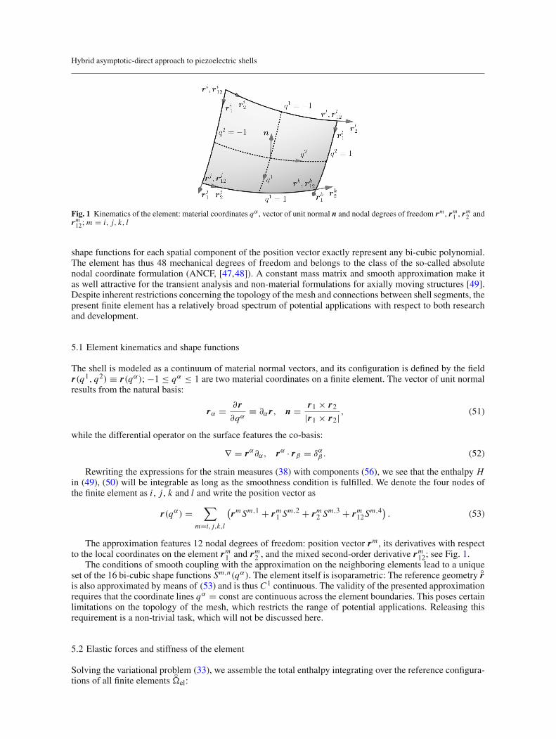
Fig. 1 Kinematics of the element: material coordinates qα , vector of unit normal n and nodal degrees of freedom rm , rm1 , rm2 and

rm12; m = i, j, k, l

shape functions for each spatial component of the position vector exactly represent any bi-cubic polynomial.The element has thus 48 mechanical degrees of freedom and belongs to the class of the so-called absolutenodal coordinate formulation (ANCF, [47,48]). A constant mass matrix and smooth approximation make itas well attractive for the transient analysis and non-material formulations for axially moving structures [49].Despite inherent restrictions concerning the topology of the mesh and connections between shell segments, thepresent finite element has a relatively broad spectrum of potential applications with respect to both researchand development.

5.1 Element kinematics and shape functions

The shell is modeled as a continuum of material normal vectors, and its configuration is defined by the fieldr(q1, q2) ≡ r(qα); −1 ≤ qα ≤ 1 are two material coordinates on a finite element. The vector of unit normalresults from the natural basis:

rα = ∂ r∂qα

≡ ∂α r, n = r1 × r2|r1 × r2|

, (51)

while the differential operator on the surface features the co-basis:

∇ = rα∂α, rα · rβ = δαβ . (52)

Rewriting the expressions for the strain measures (38) with components (56), we see that the enthalpy Hin (49), (50) will be integrable as long as the smoothness condition is fulfilled. We denote the four nodes ofthe finite element as i , j , k and l and write the position vector as

r(qα) =∑

m=i, j,k,l

(rmSm,1 + rm1 S

m,2 + rm2 Sm,3 + rm12S

m,4) . (53)

The approximation features 12 nodal degrees of freedom: position vector rm , its derivatives with respectto the local coordinates on the element rm1 and rm2 , and the mixed second-order derivative rm12; see Fig. 1.

The conditions of smooth coupling with the approximation on the neighboring elements lead to a uniqueset of the 16 bi-cubic shape functions Sm,n(qα). The element itself is isoparametric: The reference geometry ◦ris also approximated by means of (53) and is thus C1 continuous. The validity of the presented approximationrequires that the coordinate lines qα = const are continuous across the element boundaries. This poses certainlimitations on the topology of the mesh, which restricts the range of potential applications. Releasing thisrequirement is a non-trivial task, which will not be discussed here.

5.2 Elastic forces and stiffness of the element

Solving the variational problem (33), we assemble the total enthalpy integrating over the reference configura-tions of all finite elements

◦!el:

Yu. Vetyukov et al.

δHΣ = 0, HΣ =∑

Hel + Hext, Hel =∫

◦!el

H(E,K,ϕ) d◦! (54)

with Hext being the potential of external forces q and P . Unknowns are the nodal degrees of freedom andelectric voltages ϕk at open-circuit regions (sensors). This latter fact introduces additional coupling into thesystem for all elements, which belong to the same !i . This coupling results in a non-local formulation overthe domain !i , as it has been discussed in detail in [4] for a linear plate. As in (50) c > 0 and the enthalpy His not positive definite, we cannot speak about the minimality problem in the presence of electrical unknowns,but experience shows that small negative eigenvalues of the stiffness matrix do not influence the convergenceof the quasi-Newton scheme for solving the equation in (54).

Dividing the domain into finite elements, we keep in mind that the function HΣ is integrable due to thecontinuity of the approximation. Numerical results in Sect. 6 were obtained by using the Gaussian quadraturerule with 3 × 3 integration points for the integral over the element surface

◦!el in the reference configuration.

The invariant expression for H(E,K,ϕ) (50) can be written in components with the formulas

trE = Eαβ◦rα · ◦rβ = Eαβ

◦aαβ , E· ·E = EαβEγ δ◦aβγ ◦aαδ, (55)

which also holds for K = Kαβ◦rα ◦rβ , with components

Eαβ = 12

(aαβ − ◦aαβ

), Kαβ = bαβ − ◦

bαβ;

aαβ = rα · rβ , bαβ = rαβ · n, aαβ = rα · rβ . (56)

The components of the metric tensors in the reference configuration ◦aαβ ,◦bαβ shall be precomputed in the

integration points of the finite elements: They fully determine the undeformed geometry of the shell, and theelementary surface is

d◦! =

√det

{◦aαβ

}dq1 dq2. (57)

We employ the Newton method for seeking the stationary points of HΣ , for which we need the derivatives

Fel,p = −∂HΣ

∂ep, Kel,pq = ∂2HΣ

∂ep∂eq, p, q = 1 . . . N (58)

to be computable for any configuration of the shell. There are N = 48 mechanical degrees of freedom ep forfinite elements without piezoelectric properties or with prescribed electric voltage, and N = 49 for elementsin open-circuit regions, in which the electrical unknown ϕ is shared among multiple elements. The globalforce vector F and stiffness matrix K result from assembling (summation) of Fel and Kel over the integrationpoints, where the derivatives of the distributed enthalpy H(E,K,ϕ) are computed efficiently by a chain rule.

5.3 Boundary conditions

If an edge is free from kinematic constraints, then the external force factors acting on that edge need to beaccounted for. In static problems, it is common to deal with conservative loads, which allows to speak aboutthe potential energy of external force factors at the boundary. The most simple case of a conservative edge loadis a force, which is distributed per unit length of the edge in the reference configuration. This means that theforce vector P changes with the extension or contraction of the edge. The contribution of the potential energyof this force to Hext in (54) is easy to compute by integrating over the edges of the elements at the boundary.

At a simply supported edge, the particles are fixed by appropriate penalty terms for the nodal positions rmand derivatives rmα (α corresponds to the direction along the edge). If the edge is clamped, then the direction ofthe normal vector n needs to be additionally constrained. For a straight edge, n = ◦n = const, and the constraintwill be fulfilled exactly, if we demand ◦n · rmβ = 0 and ◦n · rm12 = 0, in which β corresponds to the directionpointing outwards of the domain. The same conditions can be applied at curved edges with satisfactory results.

Hybrid asymptotic-direct approach to piezoelectric shells

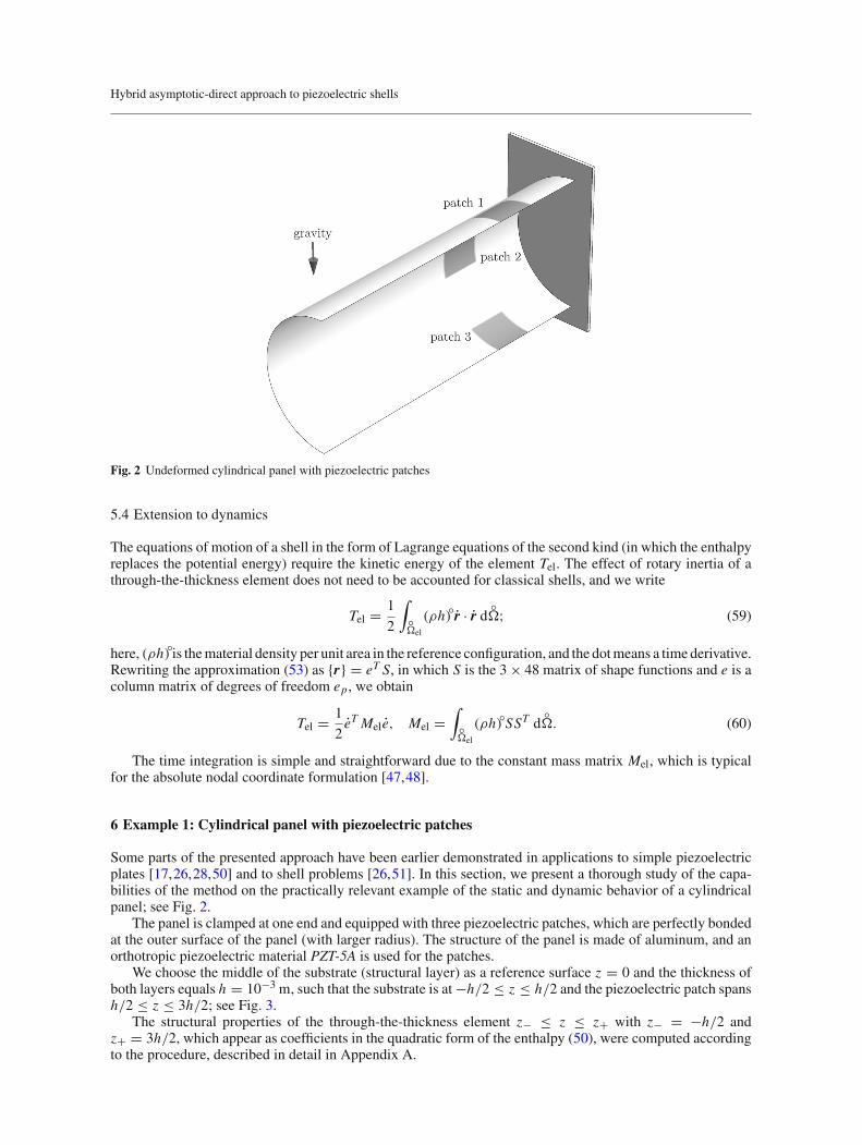
Fig. 2 Undeformed cylindrical panel with piezoelectric patches

5.4 Extension to dynamics

The equations of motion of a shell in the form of Lagrange equations of the second kind (in which the enthalpyreplaces the potential energy) require the kinetic energy of the element Tel. The effect of rotary inertia of athrough-the-thickness element does not need to be accounted for classical shells, and we write

Tel =12

∫

◦!el

(ρh)◦r · r d ◦!; (59)

here, (ρh)◦is thematerial density per unit area in the reference configuration, and the dotmeans a time derivative.Rewriting the approximation (53) as {r} = eT S, in which S is the 3× 48 matrix of shape functions and e is acolumn matrix of degrees of freedom ep, we obtain

Tel =12eT Mele, Mel =

∫

◦!el

(ρh)◦SST d◦!. (60)

The time integration is simple and straightforward due to the constant mass matrix Mel, which is typicalfor the absolute nodal coordinate formulation [47,48].

6 Example 1: Cylindrical panel with piezoelectric patches

Some parts of the presented approach have been earlier demonstrated in applications to simple piezoelectricplates [17,26,28,50] and to shell problems [26,51]. In this section, we present a thorough study of the capa-bilities of the method on the practically relevant example of the static and dynamic behavior of a cylindricalpanel; see Fig. 2.

The panel is clamped at one end and equipped with three piezoelectric patches, which are perfectly bondedat the outer surface of the panel (with larger radius). The structure of the panel is made of aluminum, and anorthotropic piezoelectric material PZT-5A is used for the patches.

We choose the middle of the substrate (structural layer) as a reference surface z = 0 and the thickness ofboth layers equals h = 10−3 m, such that the substrate is at−h/2 ≤ z ≤ h/2 and the piezoelectric patch spansh/2 ≤ z ≤ 3h/2; see Fig. 3.

The structural properties of the through-the-thickness element z− ≤ z ≤ z+ with z− = −h/2 andz+ = 3h/2, which appear as coefficients in the quadratic form of the enthalpy (50), were computed accordingto the procedure, described in detail in Appendix A.

Yu. Vetyukov et al.

piezoelectric patch

substrate

ground

ϕ

x

z

−h/2

h/2

3h/2

Fig. 3 Through-the-thickness element of the shell in the region with a piezoelectric patch

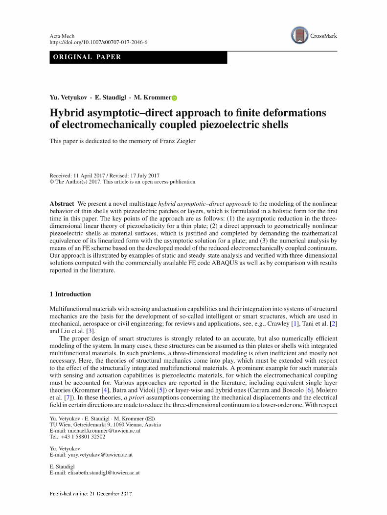
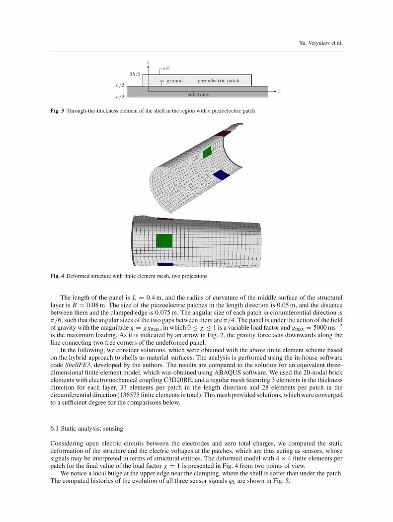
Fig. 4 Deformed structure with finite element mesh, two projections

The length of the panel is L = 0.4m, and the radius of curvature of the middle surface of the structurallayer is R = 0.08m. The size of the piezoelectric patches in the length direction is 0.05m, and the distancebetween them and the clamped edge is 0.075m. The angular size of each patch in circumferential direction isπ/6, such that the angular sizes of the two gaps between them are π/4. The panel is under the action of the fieldof gravity with the magnitude g = χgmax, in which 0 ≤ χ ≤ 1 is a variable load factor and gmax = 5000ms−2

is the maximum loading. As it is indicated by an arrow in Fig. 2, the gravity force acts downwards along theline connecting two free corners of the undeformed panel.

In the following, we consider solutions, which were obtained with the above finite element scheme basedon the hybrid approach to shells as material surfaces. The analysis is performed using the in-house softwarecode ShellFE3, developed by the authors. The results are compared to the solution for an equivalent three-dimensional finite element model, which was obtained using ABAQUS software. We used the 20-nodal brickelements with electromechanical coupling C3D20RE, and a regular mesh featuring 3 elements in the thicknessdirection for each layer, 33 elements per patch in the length direction and 28 elements per patch in thecircumferential direction (136575finite elements in total). Thismesh provided solutions,whichwere convergedto a sufficient degree for the comparisons below.

6.1 Static analysis: sensing

Considering open electric circuits between the electrodes and zero total charges, we computed the staticdeformation of the structure and the electric voltages at the patches, which are thus acting as sensors, whosesignals may be interpreted in terms of structural entities. The deformed model with 4 × 4 finite elements perpatch for the final value of the load factor χ = 1 is presented in Fig. 4 from two points of view.

We notice a local bulge at the upper edge near the clamping, where the shell is softer than under the patch.The computed histories of the evolution of all three sensor signals ϕk are shown in Fig. 5.

Hybrid asymptotic-direct approach to piezoelectric shells

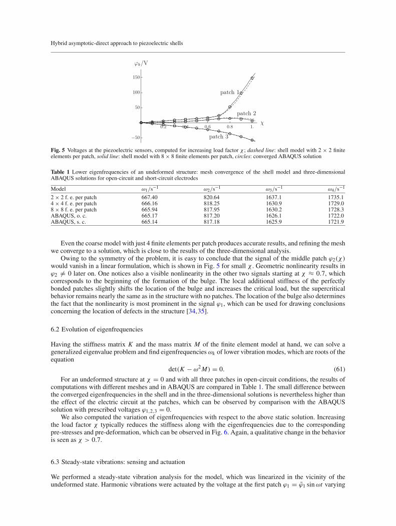
Fig. 5 Voltages at the piezoelectric sensors, computed for increasing load factor χ ; dashed line: shell model with 2 × 2 finiteelements per patch, solid line: shell model with 8 × 8 finite elements per patch, circles: converged ABAQUS solution

Table 1 Lower eigenfrequencies of an undeformed structure: mesh convergence of the shell model and three-dimensionalABAQUS solutions for open-circuit and short-circuit electrodes

Model ω1/s−1 ω2/s−1 ω3/s−1 ω4/s−1

2 × 2 f. e. per patch 667.40 820.64 1637.1 1735.14 × 4 f. e. per patch 666.16 818.25 1630.9 1729.08 × 8 f. e. per patch 665.94 817.95 1630.2 1728.3ABAQUS, o. c. 665.17 817.20 1626.1 1722.0ABAQUS, s. c. 665.14 817.18 1625.9 1721.9

Even the coarse model with just 4 finite elements per patch produces accurate results, and refining the meshwe converge to a solution, which is close to the results of the three-dimensional analysis.

Owing to the symmetry of the problem, it is easy to conclude that the signal of the middle patch ϕ2(χ)would vanish in a linear formulation, which is shown in Fig. 5 for small χ . Geometric nonlinearity results inϕ2 = 0 later on. One notices also a visible nonlinearity in the other two signals starting at χ ≈ 0.7, whichcorresponds to the beginning of the formation of the bulge. The local additional stiffness of the perfectlybonded patches slightly shifts the location of the bulge and increases the critical load, but the supercriticalbehavior remains nearly the same as in the structure with no patches. The location of the bulge also determinesthe fact that the nonlinearity is most prominent in the signal ϕ1, which can be used for drawing conclusionsconcerning the location of defects in the structure [34,35].

6.2 Evolution of eigenfrequencies

Having the stiffness matrix K and the mass matrix M of the finite element model at hand, we can solve ageneralized eigenvalue problem and find eigenfrequencies ωk of lower vibration modes, which are roots of theequation

det(K − ω2M) = 0. (61)

For an undeformed structure at χ = 0 and with all three patches in open-circuit conditions, the results ofcomputations with different meshes and in ABAQUS are compared in Table 1. The small difference betweenthe converged eigenfrequencies in the shell and in the three-dimensional solutions is nevertheless higher thanthe effect of the electric circuit at the patches, which can be observed by comparison with the ABAQUSsolution with prescribed voltages ϕ1,2,3 = 0.

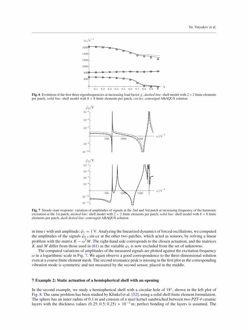
We also computed the variation of eigenfrequencies with respect to the above static solution. Increasingthe load factor χ typically reduces the stiffness along with the eigenfrequencies due to the correspondingpre-stresses and pre-deformation, which can be observed in Fig. 6. Again, a qualitative change in the behavioris seen as χ > 0.7.

6.3 Steady-state vibrations: sensing and actuation

We performed a steady-state vibration analysis for the model, which was linearized in the vicinity of theundeformed state. Harmonic vibrations were actuated by the voltage at the first patch ϕ1 = ϕ1 sinωt varying

Yu. Vetyukov et al.

Fig. 6 Evolution of the first three eigenfrequencies at increasing load factor χ ; dashed line: shell model with 2×2 finite elementsper patch, solid line: shell model with 8 × 8 finite elements per patch, circles: converged ABAQUS solution

Fig. 7 Steady-state response: variation of amplitudes of signals at the 2nd and 3rd patch at increasing frequency of the harmonicexcitation at the 1st patch; dashed line: shell model with 2 × 2 finite elements per patch, solid line: shell model with 8 × 8 finiteelements per patch, dash dotted line: converged ABAQUS solution

in time t with unit amplitude: ϕ1 = 1V.Analyzing the linearized dynamics of forced oscillations, we computedthe amplitudes of the signals ϕ2,3 sinωt at the other two patches, which acted as sensors, by solving a linearproblem with the matrix K − ω2M . The right-hand side corresponds to the chosen actuation, and the matricesK and M differ from those used in (61) as the variable ϕ1 is now excluded from the set of unknowns.

The computed variations of amplitudes of the measured signals are plotted against the excitation frequencyω in a logarithmic scale in Fig. 7. We again observe a good correspondence to the three-dimensional solutioneven at a coarse finite element mesh. The second resonance peak is missing in the first plot as the correspondingvibration mode is symmetric and not measured by the second sensor, placed in the middle.

7 Example 2: Static actuation of a hemispherical shell with an opening

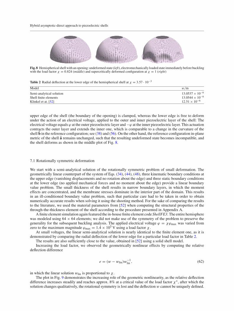
In the second example, we study a hemispherical shell with a circular hole of 18◦, shown in the left plot ofFig. 8. The same problem has been studied by Klinkel et al. [52], using a solid shell finite element formulation.The sphere has an inner radius of 0.1m and consists of a steel kernel sandwiched between two PZT-4 ceramiclayers with the thickness values (0.25; 0.5; 0.25) × 10−3 m; perfect bonding of the layers is assumed. The

Hybrid asymptotic-direct approach to piezoelectric shells

Fig. 8 Hemispherical shellwith an opening: undeformed state (left), electromechanically loaded state immediately before bucklingwith the load factor χ = 0.824 (middle) and supercritically deformed configuration at χ = 1 (right)

Table 2 Radial deflection at the lower edge of the hemispherical shell at χ = 3.57 · 10−3

Model w/m

Semi-analytical solution 13.0537 × 10−6

Shell finite elements 13.0544 × 10−6

Klinkel et at. [52] 12.51 × 10−6

upper edge of the shell (the boundary of the opening) is clamped, whereas the lower edge is free to deformunder the action of an electrical voltage, applied to the outer and inner piezoelectric layer of the shell: Theelectrical voltage equals ϕ at the outer piezoelectric layer and−ϕ at the inner piezoelectric layer. This actuationcontracts the outer layer and extends the inner one, which is comparable to a change in the curvature of theshell

◦b in the reference configuration; see (38) and (56). On the other hand, the reference configuration in-plane

metric of the shell ◦a remains unchanged, such that the resulting undeformed state becomes incompatible, andthe shell deforms as shown in the middle plot of Fig. 8.

7.1 Rotationally symmetric deformation

We start with a semi-analytical solution of the rotationally symmetric problem of small deformation. Thegeometrically linear counterpart of the system of Eqs. (34), (44), (48), three kinematic boundary conditions atthe upper edge (vanishing displacements and no rotation about the edge) and three static boundary conditionsat the lower edge (no applied mechanical forces and no moment about the edge) provide a linear boundaryvalue problem. The small thickness of the shell results in narrow boundary layers, in which the momenteffects are concentrated, and the membrane stresses dominate in the interior part of the domain. This resultsin an ill-conditioned boundary value problem, such that particular care had to be taken in order to obtainnumerically accurate results when solving it using the shooting method. For the sake of comparing the resultsto the literature, we used the material parameters from [52] when computing the structural properties of thethrough-the-thickness element of the shell according to the procedure presented in Appendix A.

Afinite element simulation again featured the in-house finite element code ShellFE3. The entire hemispherewas modeled using 64 × 64 elements; we did not make use of the symmetry of the problem to preserve thegenerality for the subsequent buckling analysis. The applied electrical voltage ϕ = χϕmax was varied fromzero to the maximum magnitude ϕmax = 1.4 × 105 V using a load factor χ .

At small voltages, the linear semi-analytical solution is nearly identical to the finite element one, as it isdemonstrated by comparing the radial deflection of the lower edge for a particular load factor in Table 2.

The results are also sufficiently close to the value, obtained in [52] using a solid shell model.Increasing the load factor, we observed the geometrically nonlinear effects by computing the relative

deflection difference

e = (w − wlin)w−1lin , (62)

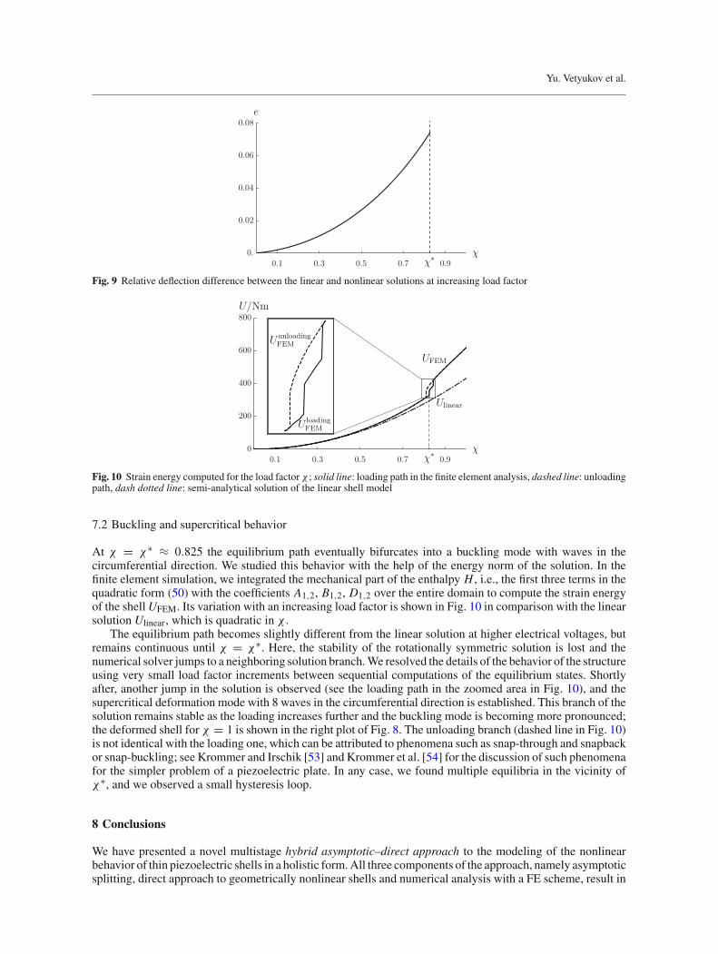
in which the linear solution wlin is proportional to χ .The plot in Fig. 9 demonstrates the increasing role of the geometric nonlinearity, as the relative deflection

difference increases steadily and reaches approx. 8% at a critical value of the load factor χ∗, after which thesolution changes qualitatively, the rotational symmetry is lost and the deflectionw cannot be uniquely defined.

Yu. Vetyukov et al.

Fig. 9 Relative deflection difference between the linear and nonlinear solutions at increasing load factor

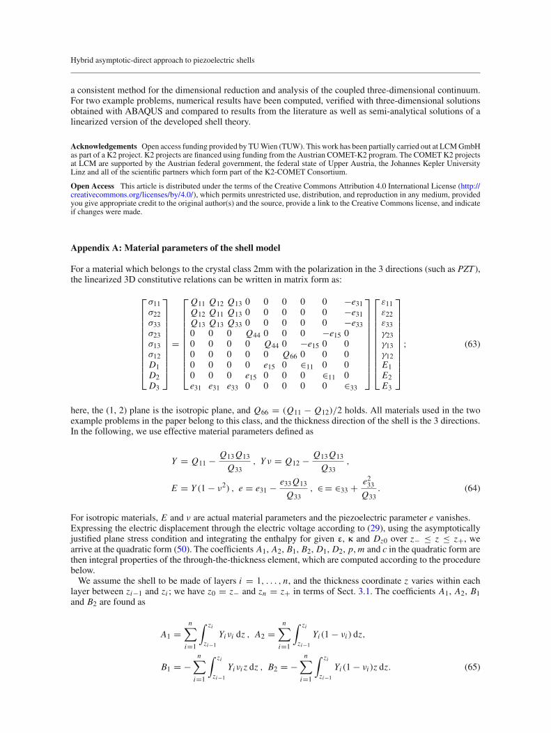
Fig. 10 Strain energy computed for the load factor χ ; solid line: loading path in the finite element analysis, dashed line: unloadingpath, dash dotted line: semi-analytical solution of the linear shell model

7.2 Buckling and supercritical behavior

At χ = χ∗ ≈ 0.825 the equilibrium path eventually bifurcates into a buckling mode with waves in thecircumferential direction. We studied this behavior with the help of the energy norm of the solution. In thefinite element simulation, we integrated the mechanical part of the enthalpy H , i.e., the first three terms in thequadratic form (50) with the coefficients A1,2, B1,2, D1,2 over the entire domain to compute the strain energyof the shellUFEM. Its variation with an increasing load factor is shown in Fig. 10 in comparison with the linearsolution Ulinear, which is quadratic in χ .

The equilibrium path becomes slightly different from the linear solution at higher electrical voltages, butremains continuous until χ = χ∗. Here, the stability of the rotationally symmetric solution is lost and thenumerical solver jumps to a neighboring solution branch.We resolved the details of the behavior of the structureusing very small load factor increments between sequential computations of the equilibrium states. Shortlyafter, another jump in the solution is observed (see the loading path in the zoomed area in Fig. 10), and thesupercritical deformation mode with 8 waves in the circumferential direction is established. This branch of thesolution remains stable as the loading increases further and the buckling mode is becoming more pronounced;the deformed shell for χ = 1 is shown in the right plot of Fig. 8. The unloading branch (dashed line in Fig. 10)is not identical with the loading one, which can be attributed to phenomena such as snap-through and snapbackor snap-buckling; see Krommer and Irschik [53] and Krommer et al. [54] for the discussion of such phenomenafor the simpler problem of a piezoelectric plate. In any case, we found multiple equilibria in the vicinity ofχ∗, and we observed a small hysteresis loop.

8 Conclusions

We have presented a novel multistage hybrid asymptotic–direct approach to the modeling of the nonlinearbehavior of thin piezoelectric shells in a holistic form.All three components of the approach, namely asymptoticsplitting, direct approach to geometrically nonlinear shells and numerical analysis with a FE scheme, result in

Hybrid asymptotic-direct approach to piezoelectric shells

a consistent method for the dimensional reduction and analysis of the coupled three-dimensional continuum.For two example problems, numerical results have been computed, verified with three-dimensional solutionsobtained with ABAQUS and compared to results from the literature as well as semi-analytical solutions of alinearized version of the developed shell theory.

Acknowledgements Open access funding provided by TUWien (TUW). This work has been partially carried out at LCMGmbHas part of a K2 project. K2 projects are financed using funding from the Austrian COMET-K2 program. The COMET K2 projectsat LCM are supported by the Austrian federal government, the federal state of Upper Austria, the Johannes Kepler UniversityLinz and all of the scientific partners which form part of the K2-COMET Consortium.

Open Access This article is distributed under the terms of the Creative Commons Attribution 4.0 International License (http://creativecommons.org/licenses/by/4.0/), which permits unrestricted use, distribution, and reproduction in any medium, providedyou give appropriate credit to the original author(s) and the source, provide a link to the Creative Commons license, and indicateif changes were made.

Appendix A: Material parameters of the shell model

For a material which belongs to the crystal class 2mm with the polarization in the 3 directions (such as PZT ),the linearized 3D constitutive relations can be written in matrix form as:

⎡

⎢⎢⎢⎢⎢⎢⎢⎢⎢⎢⎣

σ11σ22σ33σ23σ13σ12D1D2D3

⎤

⎥⎥⎥⎥⎥⎥⎥⎥⎥⎥⎦

=

⎡

⎢⎢⎢⎢⎢⎢⎢⎢⎢⎢⎣

Q11 Q12 Q13 0 0 0 0 0 −e31Q12 Q11 Q13 0 0 0 0 0 −e31Q13 Q13 Q33 0 0 0 0 0 −e330 0 0 Q44 0 0 0 −e15 00 0 0 0 Q44 0 −e15 0 00 0 0 0 0 Q66 0 0 00 0 0 0 e15 0 ∈11 0 00 0 0 e15 0 0 0 ∈11 0e31 e31 e33 0 0 0 0 0 ∈33

⎤

⎥⎥⎥⎥⎥⎥⎥⎥⎥⎥⎦

⎡

⎢⎢⎢⎢⎢⎢⎢⎢⎢⎢⎣

ε11ε22ε33γ23γ13γ12E1E2E3

⎤

⎥⎥⎥⎥⎥⎥⎥⎥⎥⎥⎦

; (63)

here, the (1, 2) plane is the isotropic plane, and Q66 = (Q11 − Q12)/2 holds. All materials used in the twoexample problems in the paper belong to this class, and the thickness direction of the shell is the 3 directions.In the following, we use effective material parameters defined as

Y = Q11 − Q13Q13

Q33, Yν = Q12 − Q13Q13

Q33,

E = Y (1 − ν2) , e = e31 − e33Q13

Q33, ∈= ∈33 +

e233Q33

. (64)

For isotropic materials, E and ν are actual material parameters and the piezoelectric parameter e vanishes.Expressing the electric displacement through the electric voltage according to (29), using the asymptoticallyjustified plane stress condition and integrating the enthalpy for given ε, κ and Dz0 over z− ≤ z ≤ z+, wearrive at the quadratic form (50). The coefficients A1, A2, B1, B2, D1, D2, p,m and c in the quadratic form arethen integral properties of the through-the-thickness element, which are computed according to the procedurebelow.We assume the shell to be made of layers i = 1, . . . , n, and the thickness coordinate z varies within each

layer between zi−1 and zi ; we have z0 = z− and zn = z+ in terms of Sect. 3.1. The coefficients A1, A2, B1and B2 are found as

A1 =n∑

i=1

∫ zi

zi−1

Yiνi dz , A2 =n∑

i=1

∫ zi

zi−1

Yi (1 − νi ) dz,

B1 = −n∑

i=1

∫ zi

zi−1

Yiνi z dz , B2 = −n∑

i=1

∫ zi

zi−1

Yi (1 − νi )z dz. (65)

Yu. Vetyukov et al.

To compute D1 and D2, we first introduce the parameters

D =n∑

i=1

∫ zi

zi−1

Yi z2 dz , Dν =n∑

i=1

∫ zi

zi−1

Yiνi z2 dz,

Dem =n∑

i=1

∫ zi

zi−1

(e2i∈i

z − 1hi

∫ zi

zi−1

e2i∈i

z dz

)

z dz ,

νD = Dν + Dem

D + Dem, hi = zi − zi−1, (66)

with the aid of which we have

D1 = (D + Dem)νD , D2 = (D + Dem)(1 − νD). (67)

Finally, we compute pi , mi and ci , which must be done for each piezoelectric layer:

pi =∫ zi

zi−1

eihi

dz = ei , mi = −∫ zi

zi−1

eihi

z dz , ci =∈i

hi. (68)

In the examples, four materials were used. The elastic material parameters for aluminum and steel are

Eal = 71 × 109 Nm−2 , νal = 0.33 ,Est = 210 × 109 Nm−2 , νst = 0.3. (69)

The material parameters for PZT-5A used in the first example are given as

Q11 = 121 × 109 Nm−2 , Q12 = 75.4 × 109 Nm−2 ,

Q13 = 75.2 × 109 Nm−2 ,

Q33 = 111 × 109 Nm−2 , Q44 = 21.1 × 109 Nm−2 ,

e31 = −5.46Cm−2 , e33 = 15.8Cm−2 , e15 = 12.32Cm−2 ,

∈11 = 1730ε0 , ∈33= 1700ε0 , ε0 = 8.854 × 10−12 A sV−1 m−1. (70)

For the dynamic simulations, we used the value of the mass density ρ = 2700 kgm−3 for aluminum andρ = 7750 kgm−3 for PZT-5A.

Concerning PZT-4 as used in the second example problem, we use the material parameters from Klinkel etal. [52], to which we compare the results of our simulations. In [52], the material was assumed mechanicallyisotropic, but still to exhibit piezoelectricity. The corresponding material parameters are

E = 81.3 × 109 Nm−2 , ν = 0.33 ,e31 = −5.203Cm−2 , e33 = 15.08Cm−2 ,

e15 = 12.72Cm−2 , ∈33= 6.752 × 10−9 A sV−1 m−1. (71)

References

1. Crawley, E.F.: Intelligent structures for aerospace: a technology overview and assessment. AIAA J. 32(8), 1689–1699 (1994)2. Tani, J., Takagi, T., Qiu, J.: Intelligent material systems: application of functional materials. Appl. Mech. Rev. 51, 505–521

(1998)3. Liu, S.-C., Tomizuka, M., Ulsoy, G.: Challenges and opportunities in the engineering of intelligent structures. Smart Struct.

Syst. 1(1), 1–12 (2005)4. Krommer, M.: The significance of non-local constitutive relations for composite thin plates including piezoelastic layers

with prescribed electric charge. Smart Mater. Struct. 12, 318–330 (2003)5. Batra, R.C., Vidoli, S.: Higher order piezoelectric plate theory derived from a three dimensional variational principle. AIAA

J. 40, 91–104 (2002)6. Carrera, E., Boscolo, M.: Classical and mixed finite elements for static and dynamic analysis of piezoelectric plates. Int. J.

Numer. Methods Eng. 70(10), 1135–1181 (2007)7. Moleiro, F., Mota Soares, C.M., Mota Soares, C.A., Reddy, J.N.: Layerwise mixed models for analysis of multilayered

piezoelectric composite plates using least-squares formulation. Compos. Struct. 119, 134–149 (2015)

Hybrid asymptotic-direct approach to piezoelectric shells

8. Zheng, S., Wang, X., Chen, W.: The formulation of a refined hybrid enhanced assumed strain solid shell element and itsapplication to model smart structures containing distributed piezoelectric sensors/actuators. Smart Mater. Struct. 13, 43–50(2004)

9. Tan, X., Vu-Quoc, L.: Optimal solid shell element for large deformable composite structures with piezoelectric layers andactive vibration control. Int. J. Numer. Methods Eng. 64, 1981–2013 (2005)

10. Klinkel, S., Wagner,W.: A piezoelectric solid shell element based on a mixed variational formulation for geometrically linearand nonlinear applications. Comput. Struct. 86, 38–46 (2008)

11. Marinkovic, D., Köppe, H., Gabbert, U.: Degenerated shell element for geometrically nonlinear analysis of thin-walledpiezoelectric active structures. Smart Mater. Struct. 17(1), 10 (2008)

12. Lentzen, S., Klosowski, P., Schmidt, R.: Geometrically nonlinear finite element simulation of smart piezolaminated platesand shells. Smart Mater. Struct. 16, 2265–2274 (2007)

13. Eliseev, V.V.: Mechanics of Deformable Solid Bodies (in Russian). St. Petersburg State Polytechnical University PublishingHouse, St. Petersburg (2006)

14. Yeliseyev, V.V., Orlov, S.G.: Asymptotic splitting in the three-dimensional problem of linear elasticity for elongated bodieswith a structure. J. Appl. Math. Mech. 63(1), 85–92 (1999)

15. Vetyukov, Y.: The theory of thin-walled rods of open profile as a result of asymptotic splitting in the problem of deformationof a noncircular cylindrical shell. J. Elast. 98(2), 141–158 (2010)

16. Vetyukov, Y.: Hybrid asymptotic–direct approach to the problem of finite vibrations of a curved layered strip. Acta Mech.223(2), 371–385 (2012)

17. Vetyukov, Y., Kuzin, A., Krommer, M.: Asymptotic splitting in the three-dimensional problem of elasticity for non-homogeneous piezoelectric plates. Int. J. Solids Struct. 48(1), 12–23 (2011)

18. Nowacki, W.: Foundations of linear piezoelectricity. In: Parkus, H. (ed.) Electromagnetic Interactions in Elastic Solids.Springer, Vienna (1979)

19. Ziegler, F.: Mechanics of Solids and Fluids. Mechanical Engineering Series, 2nd edn. Springer, Vienna (1995)20. Goldenveizer, A.L.: Theory of Elastic Thin Shells. Pergamon Press, New York (1961)21. Maugin, G.A., Attou, D.: An asymptotic theory of thin piezoelectric plates. Q. J. Mech. Appl. Math. 43, 347–362 (1990)22. Kalamkarov, A.L., Kolpakov, A.G.: A new asymptotic model for a composite piezoelastic plate. Int. J. Solids Struct. 38,

6027–6044 (2001)23. Berdichevsky, V.L.: Variational Principles of Continuum Mechanics, vol. 2. Springer, Berlin (2009)24. Wang, Y.M., Tarn, J.Q.: A three-dimensional analysis for anisotropic inhomogeneous and laminated plates. Int. J. Solids

Struct. 31, 497–515 (1994)25. Ciarlet, P.G.: Mathematical Elasticity, volume II: Theory of Plates of Studies in Mathematics and its Applications. North-

Holland, Amsterdam (1997)26. Vetyukov, Y.: Nonlinear Mechanics of Thin-Walled Structures. Asymptotics, Direct Approach and Numerical Analysis.

Foundations of Engineering Mechanics. Springer, Vienna (2014)27. Eliseev, V.V.: Mechanics of elastic bodies (in Russian). St. Petersburg State Polytechnical University Publishing House, St.

Petersburg (2003)28. Krommer, M., Irschik, H.: A Reissner–Mindlin type plate theory including the direct piezoelectric and the pyroelectric effect.

Acta Mech. 141, 51–69 (2000)29. Krommer, M.: Piezoelastic vibrations of composite Reissner–Mindlin-type plates. J. Sound Vib. 263, 871–891 (2002)30. Kulikov, G.M., Mamontov, A.A., Plotnikova, S.V.: Coupled thermoelectroelastic stress analysis of piezoelectric shells.

Compos. Struct. 124, 65–76 (2015)31. Huber, D., Krommer, M., Irschik, H.: Dynamic displacement tracking of a one-storey frame structure using patch actuator

networks: analytical plate solution and FE validation. Smart Struct. Syst. 5(6), 613–632 (2009)32. Schoeftner, J., Buchberger, G., Irschik, H.: Static and dynamic shape control of slender beams by piezoelectric actuation and

resistive electrodes. Compos. Struct. 111, 66–74 (2014)33. Krommer, M., Irschik, H.: Sensor and actuator design for displacement control of continuous systems. Smart Struct. Syst.

3(2), 147–172 (2007)34. Krommer,M.,Vetyukov,Y.:Adaptive sensing of kinematic entities in the vicinity of a time-dependent geometrically nonlinear

pre-deformed state. Int. J. Solids Struct. 46(17), 3313–3320 (2009)35. Vetyukov, Y., Krommer, M.: Optimal continuous strain-type sensors for finite deformations of shell structures. Mech. Adv.

Mater. Struct. 18(2), 125–132 (2011)36. Eliseev, V.V., Vetyukov, Y.: Finite deformation of thin shells in the context of analytical mechanics of material surfaces. Acta

Mech. 209(1–2), 43–57 (2010)37. Eliseev, V., Vetyukov, Y.: Theory of shells as a product of analytical technologies in elastic body mechanics. In:

Pietraszkiewicz, W., Górski, J. (eds.) Shell Structures: Theory and Applications, vol. 3, pp. 81–84. CRC Press, Balkema(2014)

38. Ciarlet, P.G.: An introduction to differential geometry with applications to elasticity. J. Elast. 1–3(78/79), 1–215 (2005)39. Stoker, J.J.: Differential Geometry. Wiley, Wiley Classics Library (1989). (ISBN: 9780471504030)40. Marinkovic, D., Köppe, H., Gabbert, U.: Aspects of modeling piezoelectric active thin-walled structures. J. Intell. Mater.

Syst. Struct. 20(15), 1835–1844 (2009)41. Zhang, S.-Q., Li, Y.-X., Schmidt, R.: Active shape and vibration control for piezoelectric bonded composite structures using

various geometric nonlinearities. Compos. Struct. 122, 239–249 (2015)42. Vetyukov, Y.: Finite element modeling of Kirchhoff-Love shells as smooth material surfaces. ZAMM 94(1–2), 150–163

(2014)43. Ivannikov, V., Tiago, C., Pimenta, P.M.: Meshless implementation of the geometrically exact Kirchhoff–Love shell theory.

Int. J. Numer. Methods Eng. 100, 1–39 (2014)44. Kiendl, J., Bletzinger, K.-U., Linhard, J., Wüchner, R.: Isogeometric shell analysis with Kirchhoff–Love elements. Comput.

Methods Appl. Mech. Eng. 198(49–52), 3902–3914 (2009). (ISSN: 0045-7825)

Yu. Vetyukov et al.

45. Cirak, F., Ortiz, M.: Fully C1-conforming subdivision elements for finite deformation thin-shell analysis. Int. J. Numer.Methods Eng. 51, 813–833 (2001)

46. Bogner, F.K., Fox, R.L., Schmit, L.A.: The generation of interelement compatible stiffness and mass matrices by the use ofinterpolation formulae. In: Proceedings of the 1st Conference on Matrix Methods in Structural Mechanics, volume AFFDL-TR-66-80, pp. 397–443, Wright Patterson Air force Base, Ohio (1966)

47. Shabana, A.A.: Computational Continuum Mechanics. Cambridge University Press, Cambridge (2008)48. Gruber, P.G., Nachbagauer, K., Vetyukov, Y., Gerstmayr, J.: A novel director-based Bernoulli–Euler beam finite element in

absolute nodal coordinate formulation free of geometric singularities. Mech. Sci. 4, 279–289 (2013)49. Vetyukov, Y., Gruber, P.G., Krommer, M.: Nonlinear model of an axially moving plate in a mixed Eulerian-Largangian

framework. Acta Mech. 227, 2831–2842 (2016). https://doi.org/10.1007/s00707-016-1651-050. Vetyukov, Y., Krommer, M.: On the combination of asymptotic and direct approaches to the modeling of plates with

piezoelectric actuators and sensors. In: Proceedings of SPIE—The International Society for Optical Engineering, vol. 7647(2010)

51. Krommer,M., Pieber,M., Vetyukov, Y.:Modellierung, Simulation und Schwingungsreduktion dünner Schalenmit piezoelek-trischen Wandlern. Elektrotechnik & Informationstechnik 132(8), 437–447 (2015)

52. Klinkel, S., Wagner, W.: A geometrically non-linear piezoelectric solid shell element based on a mixed multi-field variationalformulation. Int. J. Numer. Methods Eng. 65(3), 349–382 (2006)

53. Krommer, M., Irschik, H.: Post-buckling of piezoelectric thin plates. Int. J. Struct. Stab. Dyn. 15(7), 21p (2015)54. Krommer, M., Vetyukov, Y., Staudigl, E.: Nonlinear modelling and analysis of thin piezoelectric plates: buckling and post-

buckling behaviour. Smart Struct. Syst. 18(1), 155–181 (2016)