EECS 70 Discrete Mathematics and Probability TheorySpring 2014 Anant Sahai Homework 15This homework is entirely optional. We will post solutions on May 12 2014.

1. Cal Basketball (this problem is in-scope for the final)The Cal basketball team plays 100 independent games, each of which they have probability 0.8 of winning. Use theCentral Limit Theorem and the table at the end of this HW to estimate the probability that they win at least 90 games.

2. Expecting you to integrate by parts!In Discussion 12B, we derived an alternative form for the expected value of a discrete non-negative random variableY , E[Y ] = ∑

∞i=1 P(Y ≥ i), when Y takes on values from 1 to n. In this problem, we will derive the continuous analog of

this expression. Throughout this problem, assume X is a continuous non-negative random variable with PDF fX (x).

(a) Write an expression for P(X ≥ x) in terms of fX (x). This is called the complementary cumulative distributionfunction of X , of the CDF of X . For this problem, we denote this as F̄X (x). What is F̄X (0)? How about F̄X (x) asx→ ∞?

(b) Use integration by parts on E[X ] =∫

∞

0 x fX (x) dx to derive the expression in question. (Hint: What is theantiderivative of fX (x)? )

3. Exponential worldIn lecture you learned about exponential random variables. If X is a non-negative and continuous random variable, wecall it an exponential random variable with rate λ if and only if for each t ≥ 0 we have Pr[X ≥ t] = e−λ t .

(a) Show that an exponential random variable is memoryless. This means that Pr[X ≥ t1 + t2|X ≥ t2] = Pr[X ≥ t1].Why does this property justify the use of an exponential random variable to approximately model the following:the length of the time it takes from now until the next customer arrives in a shop?

(b) Now consider a shop. Customers are arriving in the shop. We model them this way: the first customer drawsa sample from the exponential distribution with rate 1 and arrives at the time specified by that. The secondcustomer independently draws another sample from the exponential distribution and waits that much time aftercustomer 1 before arriving at the shop, and so on.Now assume that the random variable the first customer draws is X1 and the one that the second customer drawsis X2. Therefore the first customer arrives at time X1 and the second customer arrives at time X1 +X2.The shop owner is a psychic and knows that in the next hour, there is exactly one customer arriving. So X1 < 1and X1 +X2 > 1. Conditioned on this we wish to figure the distribution of X1.Fix a tiny interval [t, t + ε] for some t ∈ [0,1] and some small ε > 0. What is Pr[X1 ∈ [t, t + ε]]?

(c) Conditioned on X1 ∈ [t, t + ε], the probability of the event X1 +X2 > 1 is roughly equivalent to the probability ofX2 > 1−t (this approximation becomes more and more accurate as ε→ 0). Use this to approximate Pr[X1+X2 >1|X1 ∈ [t, t + ε]].

(d) Now use the Bayes formula to compute Pr[X1 ∈ [t, t + ε]|X1 +X2 > 1]. Does the result depend on t? Argue thatthe distribution of X1 conditioned on the fact that X1 +X2 > 1 and X1 < 1 is uniform on [0,1].

4. Exponential Distributions: LightbulbsA brand new lightbulb has just been installed in our classroom, and you know the life span of a lightbulb is exponen-tially distributed with a mean of 50 days.

EECS 70, Spring 2014, Homework 15 1

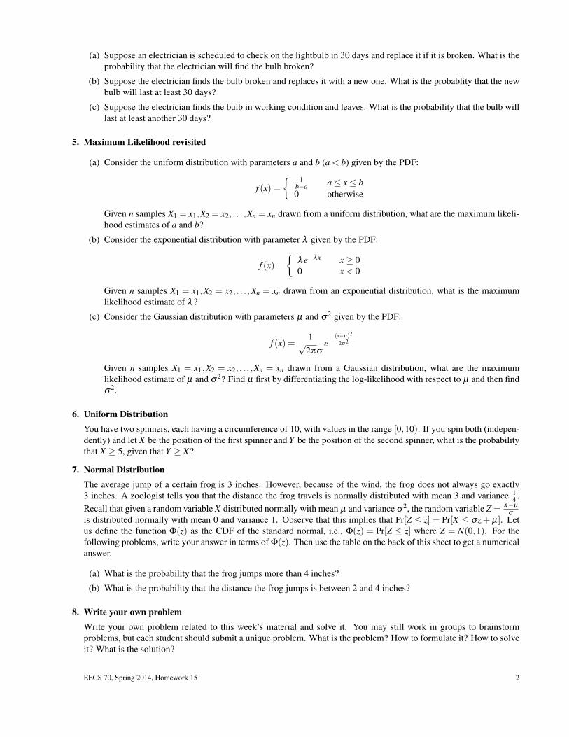
(a) Suppose an electrician is scheduled to check on the lightbulb in 30 days and replace it if it is broken. What is theprobability that the electrician will find the bulb broken?

(b) Suppose the electrician finds the bulb broken and replaces it with a new one. What is the probablity that the newbulb will last at least 30 days?

(c) Suppose the electrician finds the bulb in working condition and leaves. What is the probability that the bulb willlast at least another 30 days?

5. Maximum Likelihood revisited

(a) Consider the uniform distribution with parameters a and b (a < b) given by the PDF:

f (x) ={ 1

b−a a≤ x≤ b0 otherwise

Given n samples X1 = x1,X2 = x2, . . . ,Xn = xn drawn from a uniform distribution, what are the maximum likeli-hood estimates of a and b?

(b) Consider the exponential distribution with parameter λ given by the PDF:

f (x) ={

λe−λx x≥ 00 x < 0

Given n samples X1 = x1,X2 = x2, . . . ,Xn = xn drawn from an exponential distribution, what is the maximumlikelihood estimate of λ?

(c) Consider the Gaussian distribution with parameters µ and σ2 given by the PDF:

f (x) =1√

2πσe−

(x−µ)2

2σ2

Given n samples X1 = x1,X2 = x2, . . . ,Xn = xn drawn from a Gaussian distribution, what are the maximumlikelihood estimate of µ and σ2? Find µ first by differentiating the log-likelihood with respect to µ and then findσ2.

6. Uniform DistributionYou have two spinners, each having a circumference of 10, with values in the range [0,10). If you spin both (indepen-dently) and let X be the position of the first spinner and Y be the position of the second spinner, what is the probabilitythat X ≥ 5, given that Y ≥ X?

7. Normal DistributionThe average jump of a certain frog is 3 inches. However, because of the wind, the frog does not always go exactly3 inches. A zoologist tells you that the distance the frog travels is normally distributed with mean 3 and variance 1

4 .Recall that given a random variable X distributed normally with mean µ and variance σ2, the random variable Z = X−µ

σ

is distributed normally with mean 0 and variance 1. Observe that this implies that Pr[Z ≤ z] = Pr[X ≤ σz+ µ]. Letus define the function Φ(z) as the CDF of the standard normal, i.e., Φ(z) = Pr[Z ≤ z] where Z = N(0,1). For thefollowing problems, write your answer in terms of Φ(z). Then use the table on the back of this sheet to get a numericalanswer.

(a) What is the probability that the frog jumps more than 4 inches?

(b) What is the probability that the distance the frog jumps is between 2 and 4 inches?

8. Write your own problemWrite your own problem related to this week’s material and solve it. You may still work in groups to brainstormproblems, but each student should submit a unique problem. What is the problem? How to formulate it? How to solveit? What is the solution?

EECS 70, Spring 2014, Homework 15 2

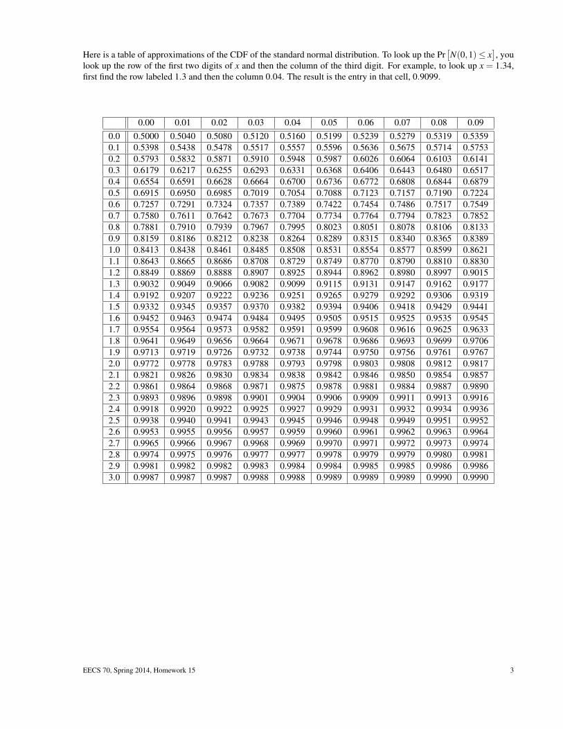
Here is a table of approximations of the CDF of the standard normal distribution. To look up the Pr[N(0,1)≤ x

], you

look up the row of the first two digits of x and then the column of the third digit. For example, to look up x = 1.34,first find the row labeled 1.3 and then the column 0.04. The result is the entry in that cell, 0.9099.

0.00 0.01 0.02 0.03 0.04 0.05 0.06 0.07 0.08 0.090.0 0.5000 0.5040 0.5080 0.5120 0.5160 0.5199 0.5239 0.5279 0.5319 0.53590.1 0.5398 0.5438 0.5478 0.5517 0.5557 0.5596 0.5636 0.5675 0.5714 0.57530.2 0.5793 0.5832 0.5871 0.5910 0.5948 0.5987 0.6026 0.6064 0.6103 0.61410.3 0.6179 0.6217 0.6255 0.6293 0.6331 0.6368 0.6406 0.6443 0.6480 0.65170.4 0.6554 0.6591 0.6628 0.6664 0.6700 0.6736 0.6772 0.6808 0.6844 0.68790.5 0.6915 0.6950 0.6985 0.7019 0.7054 0.7088 0.7123 0.7157 0.7190 0.72240.6 0.7257 0.7291 0.7324 0.7357 0.7389 0.7422 0.7454 0.7486 0.7517 0.75490.7 0.7580 0.7611 0.7642 0.7673 0.7704 0.7734 0.7764 0.7794 0.7823 0.78520.8 0.7881 0.7910 0.7939 0.7967 0.7995 0.8023 0.8051 0.8078 0.8106 0.81330.9 0.8159 0.8186 0.8212 0.8238 0.8264 0.8289 0.8315 0.8340 0.8365 0.83891.0 0.8413 0.8438 0.8461 0.8485 0.8508 0.8531 0.8554 0.8577 0.8599 0.86211.1 0.8643 0.8665 0.8686 0.8708 0.8729 0.8749 0.8770 0.8790 0.8810 0.88301.2 0.8849 0.8869 0.8888 0.8907 0.8925 0.8944 0.8962 0.8980 0.8997 0.90151.3 0.9032 0.9049 0.9066 0.9082 0.9099 0.9115 0.9131 0.9147 0.9162 0.91771.4 0.9192 0.9207 0.9222 0.9236 0.9251 0.9265 0.9279 0.9292 0.9306 0.93191.5 0.9332 0.9345 0.9357 0.9370 0.9382 0.9394 0.9406 0.9418 0.9429 0.94411.6 0.9452 0.9463 0.9474 0.9484 0.9495 0.9505 0.9515 0.9525 0.9535 0.95451.7 0.9554 0.9564 0.9573 0.9582 0.9591 0.9599 0.9608 0.9616 0.9625 0.96331.8 0.9641 0.9649 0.9656 0.9664 0.9671 0.9678 0.9686 0.9693 0.9699 0.97061.9 0.9713 0.9719 0.9726 0.9732 0.9738 0.9744 0.9750 0.9756 0.9761 0.97672.0 0.9772 0.9778 0.9783 0.9788 0.9793 0.9798 0.9803 0.9808 0.9812 0.98172.1 0.9821 0.9826 0.9830 0.9834 0.9838 0.9842 0.9846 0.9850 0.9854 0.98572.2 0.9861 0.9864 0.9868 0.9871 0.9875 0.9878 0.9881 0.9884 0.9887 0.98902.3 0.9893 0.9896 0.9898 0.9901 0.9904 0.9906 0.9909 0.9911 0.9913 0.99162.4 0.9918 0.9920 0.9922 0.9925 0.9927 0.9929 0.9931 0.9932 0.9934 0.99362.5 0.9938 0.9940 0.9941 0.9943 0.9945 0.9946 0.9948 0.9949 0.9951 0.99522.6 0.9953 0.9955 0.9956 0.9957 0.9959 0.9960 0.9961 0.9962 0.9963 0.99642.7 0.9965 0.9966 0.9967 0.9968 0.9969 0.9970 0.9971 0.9972 0.9973 0.99742.8 0.9974 0.9975 0.9976 0.9977 0.9977 0.9978 0.9979 0.9979 0.9980 0.99812.9 0.9981 0.9982 0.9982 0.9983 0.9984 0.9984 0.9985 0.9985 0.9986 0.99863.0 0.9987 0.9987 0.9987 0.9988 0.9988 0.9989 0.9989 0.9989 0.9990 0.9990

EECS 70, Spring 2014, Homework 15 3