HW #4: Dimensional Analysis, Pipe Flow, Boundary Layer ...fmeabj.lecturer.eng.chula.ac.th/2142-242 HP/242 Course Materials... · Munson B. R., Young, D. F., and Okiishi, T. H., 2002,

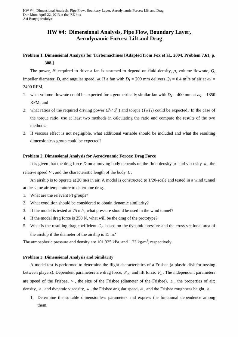
HW #4: Dimensional Analysis, Pipe Flow, Boundary Layer, Aerodynamic Forces: Lift and Drag Due Mon, April 22, 2013 at the ISE box Asi Bunyajitradulya

HW #4: Dimensional Analysis, Pipe Flow, Boundary Layer, Aerodynamic Forces: Lift and Drag

Problem 1. Dimensional Analysis for Turbomachines [Adapted from Fox et al., 2004, Problem 7.61, p.

308.]

The power, P, required to drive a fan is assumed to depend on fluid density, , volume flowrate, Q,

impeller diameter, D, and angular speed, . If a fan with D1 = 200 mm delivers Q1 = 0.4 m3/s of air at 1 =

2400 RPM,

1. what volume flowrate could be expected for a geometrically similar fan with D2 = 400 mm at 2 = 1850

RPM, and

2. what ratios of the required driving power (P2/ P1) and torque (T2/T1) could be expected? In the case of

the torque ratio, use at least two methods in calculating the ratio and compare the results of the two

methods.

3. If viscous effect is not negligible, what additional variable should be included and what the resulting

dimensionless group could be expected?

Problem 2. Dimensional Analysis for Aerodynamic Forces: Drag Force

It is given that the drag force D on a moving body depends on the fluid density and viscosity , the

relative speed V , and the characteristic length of the body L .

An airship is to operate at 20 m/s in air. A model is constructed to 1/20-scale and tested in a wind tunnel

at the same air temperature to determine drag.

1. What are the relevant PI groups?

2. What condition should be considered to obtain dynamic similarity?

3. If the model is tested at 75 m/s, what pressure should be used in the wind tunnel?

4. If the model drag force is 250 N, what will be the drag of the prototype?

5. What is the resulting drag coefficient DC based on the dynamic pressure and the cross sectional area of

the airship if the diameter of the airship is 15 m?

The atmospheric pressure and density are 101.325 kPa. and 1.23 kg/m3, respectively.

Problem 3. Dimensional Analysis and Similarity

A model test is performed to determine the flight characteristics of a Frisbee (a plastic disk for tossing

between players). Dependent parameters are drag force, DF , and lift force, LF . The independent parameters

are speed of the Frisbee, V , the size of the Frisbee (diameter of the Frisbee), D , the properties of air;

density, , and dynamic viscosity, , the Frisbee angular speed, , and the Frisbee roughness height, h .

1. Determine the suitable dimensionless parameters and express the functional dependence among

them.


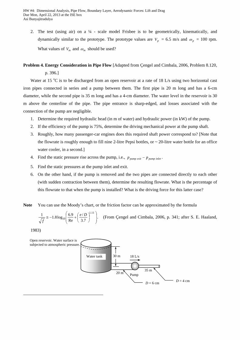
2. The test (using air) on a ¼ - scale model Frisbee is to be geometrically, kinematically, and

dynamically similar to the prototype. The prototype values are pV = 6.5 m/s and p = 100 rpm.

What values of mV and m should be used?

Problem 4. Energy Consideration in Pipe Flow [Adapted from Çengel and Cimbala, 2006, Problem 8.120,

p. 396.]

Water at 15 oC is to be discharged from an open reservoir at a rate of 18 L/s using two horizontal cast

iron pipes connected in series and a pump between them. The first pipe is 20 m long and has a 6-cm

diameter, while the second pipe is 35 m long and has a 4-cm diameter. The water level in the reservoir is 30

m above the centerline of the pipe. The pipe entrance is sharp-edged, and losses associated with the

connection of the pump are negligible.

1. Determine the required hydraulic head (in m of water) and hydraulic power (in kW) of the pump.

2. If the efficiency of the pump is 75%, determine the driving mechanical power at the pump shaft.

3. Roughly, how many passenger-car engines does this required shaft power correspond to? [Note that

the flowrate is roughly enough to fill nine 2-litre Pepsi bottles, or ~ 20-litre water bottle for an office

water cooler, in a second.]

4. Find the static pressure rise across the pump, i.e., inletpumpexitpump pp .

5. Find the static pressures at the pump inlet and exit.

6. On the other hand, if the pump is removed and the two pipes are connected directly to each other

(with sudden contraction between them), determine the resulting flowrate. What is the percentage of

this flowrate to that when the pump is installed? What is the driving force for this latter case?

Note You can use the Moody’s chart, or the friction factor can be approximated by the formula

11.1

10 7.3

/

Re

9.6log8.1

1 De

f. (From Çengel and Cimbala, 2006, p. 341; after S. E. Haaland,

1983)

Water tank 30 m

35 m 20 m

18 L/s

Pump

D = 6 cm D = 4 cm

Open reservoir. Water surface is subjected to atmospheric pressure.


Problem 5. Aerodynamic Forces

1. Find the lift-to-drag force ratio of an NACA 64(1)-412 airfoil at an angle of attack of 0o and Re ~ 106.

Also find the direction (angle measured from the drag direction) of the resultant aerodynamic force on

the airfoil.

2.

2.1. Estimate the drag force D on a smooth sphere of diameter 0.1 m that travels at a constant speed of

10 m/s in standard atmospheric air. What is the minimum power P required to sustain the

atmospheric flight of the sphere? (Minimum power here means the power that is required to propel

the sphere in the atmospheric flight only, excluding the efficiency of the propulsive device itself.)

2.2. Compare the drag force and the power to the case in which the sphere is traveling at 100 m/s by

finding the drag force ratio D(at 100 m/s) / D(at 10 m/s) and the power ratio P(at 100 m/s) / P(at 10

m/s).

2.3. If the drag coefficient does not vary with the Reynolds number and is constant, how does the power

P required vary with the speed V? Do the powers in the two cases above follow this trend? Explain.

Problem 6. Displacement and Momentum Thicknesses

1. Determine the relative displacement and momentum thicknesses, /* and / , of a boundary layer

with

the parabolic profile:

1,1

10,22

U

uf ,

and the 1-7 power law profile:

1,1

7,10,;

/1 n

U

unf

n

where u is the x-component of flow velocity, U is freestream velocity, and is boundary layer thickness.

2. For the same thickness , which profile of the two has more mass and momentum flux deficits?

Problem 7. Aerodynamic Forces

1. Estimate the drag forces on a Honda Civic at the speeds V of 60 and 120 km/h. Also, find the

required powers to drive it against the air resistance at these speeds.

Note: Try to find the information on the drag coefficient of a Civic, or a typical modern car.

2. If there is a wind at the speed wV of 30 km/h in the direction as shown below, find the total

aerodynamic force on the car at the speed of 60 km/h. Assume that the force coefficient does not

change much. In addition, also find the total power dissipated due to the air resistance.

3. Compare and discuss the results of 1 and 2.

wV

V


Appendix: Figures of External Flow, and Lift and Drag Coefficients for Various Bodies, with Brief Descriptions

References The figures and data below are from

1. Munson B. R., Young, D. F., and Okiishi, T. H., 2002, Fundamentals of Fluid Mechanics, Fourth Edition, Wiley, New York.

Some of these are after 2. Blevins, R. D., 1984, Applied Fluid Dynamics Handbook, Van Nostrand Reinhold, New York. 3. Schlichting, H., 1979, Boundary Layer Theory, Seventh Edition, McGraw-Hill, New York. 4. White, F. M., 1986, Fluid Mechanics, McGraw-Hill, New York. 5. Vennard, J. K., and Street, R. L., 1982, Elementary Fluid Mechanics, Sixth Edition, Wiley, New York. 6. Hoerner, S. F., 1965, Fluid-Dynamic Drag, published by the author, Library of Congress No. 64, 19666. 7. Vogel, J., 1994, Life in Moving Fluids, Second Edition, Willard Grant Press, Boston. 8. Gross, A. C., Kyle, C. R., and Malewicki, D. J., 1983, The Aerodynamics of Human Powered Land Vehicles,

Scientific American, Vol. 29, No. 6. 9. Abbott, I. H., von Doenhoff, A. E., and Stivers, L. S., 1945, Summary of Airfoil Data, NACA Report No. 824,

Langley Field, Va. 10. Abbott, I. H., and von Doenhoff, A. E., 1959, Theory of Wing Sections, Dover Publications, New York. 11. Goldstein, S., 1938, Modern Developments in Fluid Dynamics, Oxford Press, London.


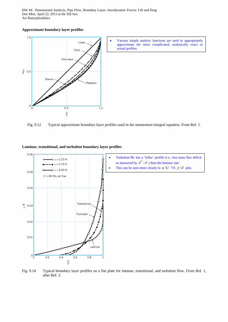
Approximate boundary layer profiles

Fig. 9.12 Typical approximate boundary layer profiles used in the momentum integral equation. From Ref. 1.

Laminar, transitional, and turbulent boundary layer profiles

Fig. 9.14 Typical boundary layer profiles on a flat plate for laminar, transitional, and turbulent flow. From Ref. 1,

after Ref. 3.

Various simple analytic functions are used to appropriately approximate the more complicated, analytically exact or actual profiles.

Turbulent BL has a ‘fuller’ profile (i.e., less mass flux deficit

as measured by /* ) than the laminar one.

This can be seen more clearly in Uu / VS /y plot.


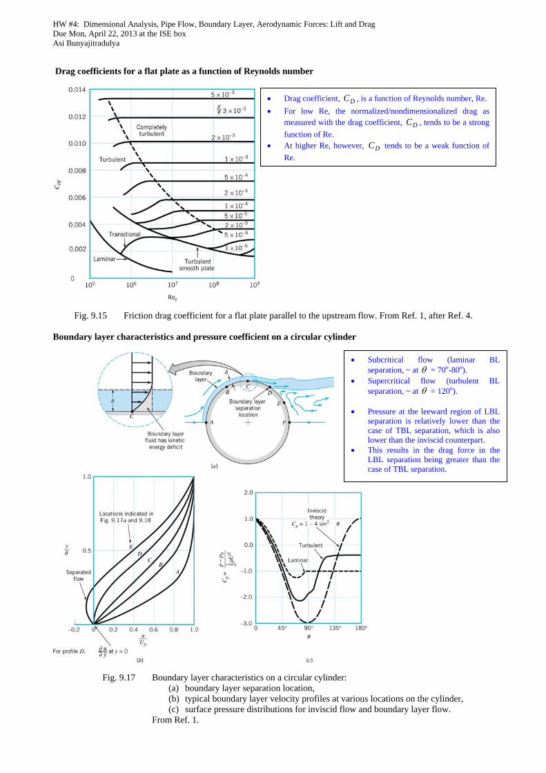
Drag coefficients for a flat plate as a function of Reynolds number

Fig. 9.15 Friction drag coefficient for a flat plate parallel to the upstream flow. From Ref. 1, after Ref. 4.

Boundary layer characteristics and pressure coefficient on a circular cylinder

Fig. 9.17 Boundary layer characteristics on a circular cylinder:

(a) boundary layer separation location, (b) typical boundary layer velocity profiles at various locations on the cylinder, (c) surface pressure distributions for inviscid flow and boundary layer flow.

From Ref. 1.

Drag coefficient, DC , is a function of Reynolds number, Re.

For low Re, the normalized/nondimensionalized drag as measured with the drag coefficient, DC , tends to be a strong

function of Re. At higher Re, however, DC tends to be a weak function of

Re.

Subcritical flow (laminar BL separation, ~ at = 70o-80o).

Supercritical flow (turbulent BL separation, ~ at = 120o).

Pressure at the leeward region of LBL

separation is relatively lower than the case of TBL separation, which is also lower than the inviscid counterpart.

This results in the drag force in the LBL separation being greater than the case of TBL separation.


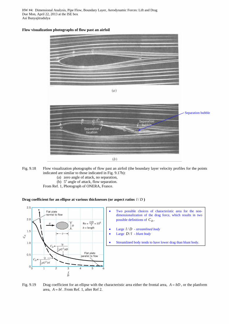
Flow visualization photographs of flow past an airfoil

Fig. 9.18 Flow visualization photographs of flow past an airfoil (the boundary layer velocity profiles for the points

indicated are similar to those indicated in Fig. 9.17b): (a) zero angle of attack, no separation, (b) 5o angle of attack, flow separation.

From Ref. 1, Photograph of ONERA, France.

Drag coefficient for an ellipse at various thicknesses (or aspect ratios Dl / )

Fig. 9.19 Drag coefficient for an ellipse with the characteristic area either the frontal area, bDA , or the planform

area, blA . From Ref. 1, after Ref 2.

Separation bubble

Two possible choices of characteristic area for the non-dimensionalization of the drag force, which results in two possible definitions of DC .

Large Dl / - streamlined body Large lD / - blunt body Streamlined body tends to have lower drag than blunt body.


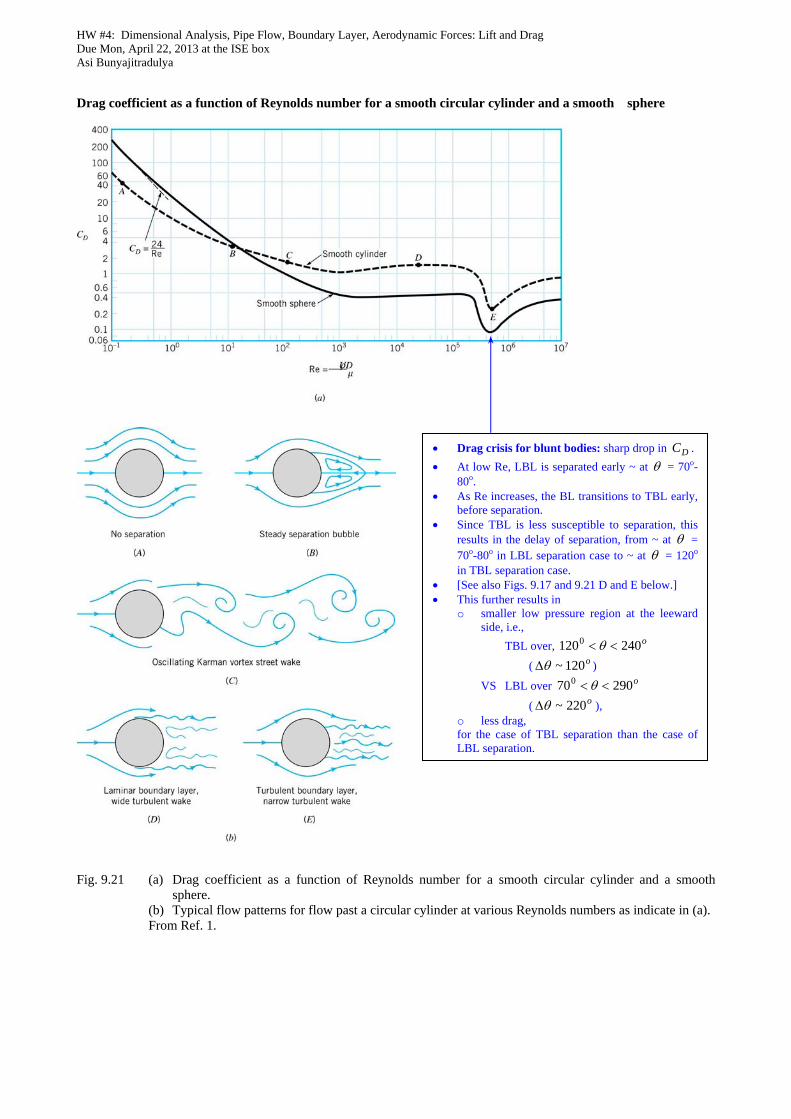
Drag coefficient as a function of Reynolds number for a smooth circular cylinder and a smooth sphere

Fig. 9.21 (a) Drag coefficient as a function of Reynolds number for a smooth circular cylinder and a smooth sphere.

(b) Typical flow patterns for flow past a circular cylinder at various Reynolds numbers as indicate in (a). From Ref. 1.

Drag crisis for blunt bodies: sharp drop in DC .

At low Re, LBL is separated early ~ at = 70o-80o.

As Re increases, the BL transitions to TBL early, before separation.

Since TBL is less susceptible to separation, this results in the delay of separation, from ~ at = 70o-80o in LBL separation case to ~ at = 120o in TBL separation case.

[See also Figs. 9.17 and 9.21 D and E below.] This further results in

o smaller low pressure region at the leeward side, i.e.,

TBL over, o2401200

( o120~ )

VS LBL over o290700

( o220~ ), o less drag, for the case of TBL separation than the case of LBL separation.


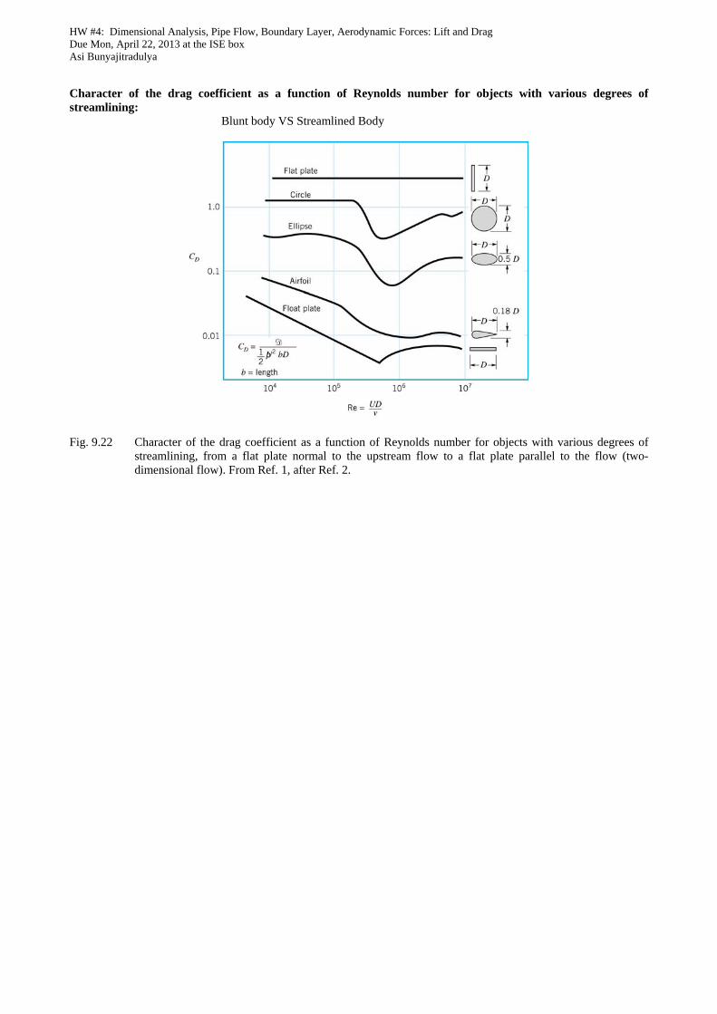
Character of the drag coefficient as a function of Reynolds number for objects with various degrees of streamlining:

Blunt body VS Streamlined Body

Fig. 9.22 Character of the drag coefficient as a function of Reynolds number for objects with various degrees of

streamlining, from a flat plate normal to the upstream flow to a flat plate parallel to the flow (two-dimensional flow). From Ref. 1, after Ref. 2.


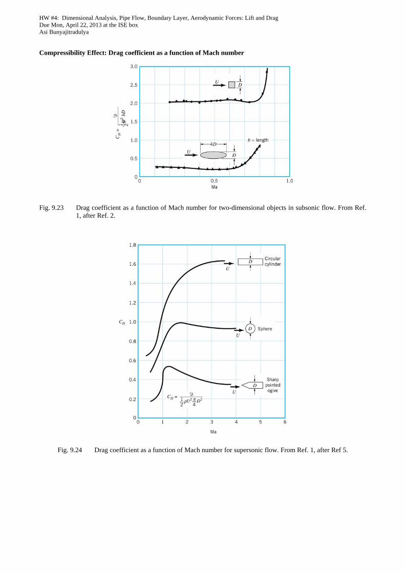
Compressibility Effect: Drag coefficient as a function of Mach number

Fig. 9.23 Drag coefficient as a function of Mach number for two-dimensional objects in subsonic flow. From Ref.

1, after Ref. 2.

Fig. 9.24 Drag coefficient as a function of Mach number for supersonic flow. From Ref. 1, after Ref 5.


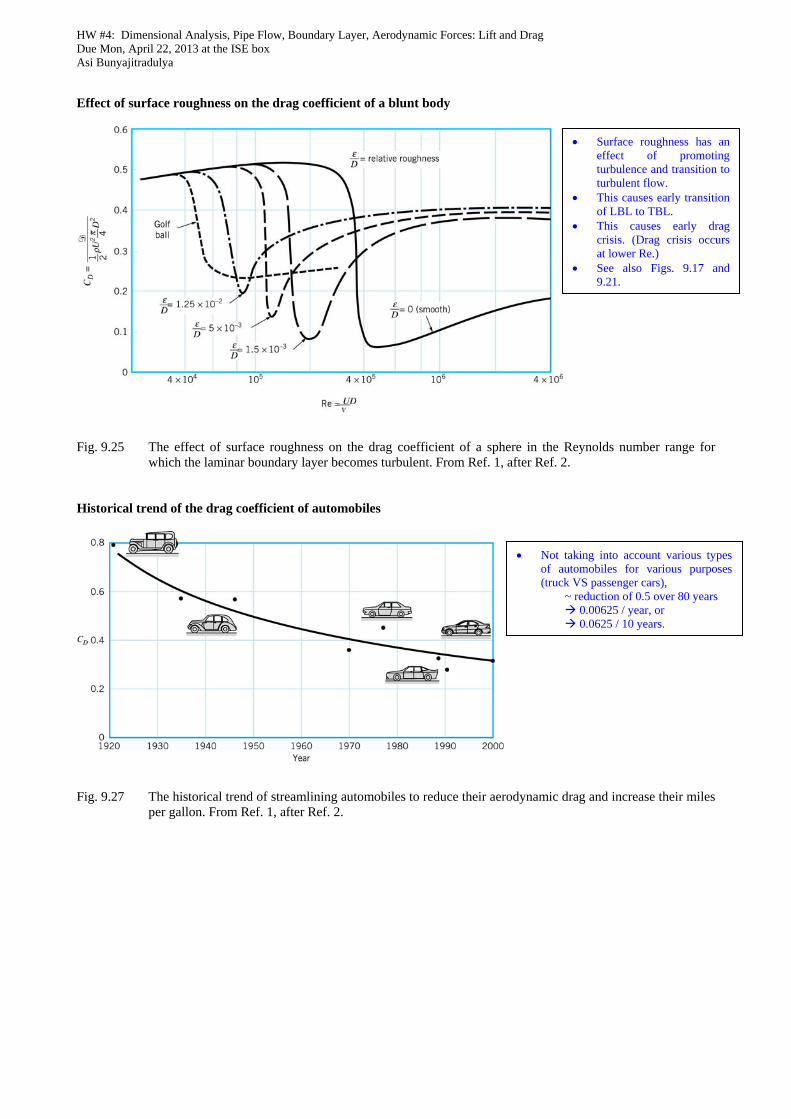
Effect of surface roughness on the drag coefficient of a blunt body

Fig. 9.25 The effect of surface roughness on the drag coefficient of a sphere in the Reynolds number range for

which the laminar boundary layer becomes turbulent. From Ref. 1, after Ref. 2. Historical trend of the drag coefficient of automobiles

Fig. 9.27 The historical trend of streamlining automobiles to reduce their aerodynamic drag and increase their miles

per gallon. From Ref. 1, after Ref. 2.

Surface roughness has an effect of promoting turbulence and transition to turbulent flow.

This causes early transition of LBL to TBL.

This causes early drag crisis. (Drag crisis occurs at lower Re.)

See also Figs. 9.17 and 9.21.

Not taking into account various types of automobiles for various purposes (truck VS passenger cars),

~ reduction of 0.5 over 80 years 0.00625 / year, or 0.0625 / 10 years.


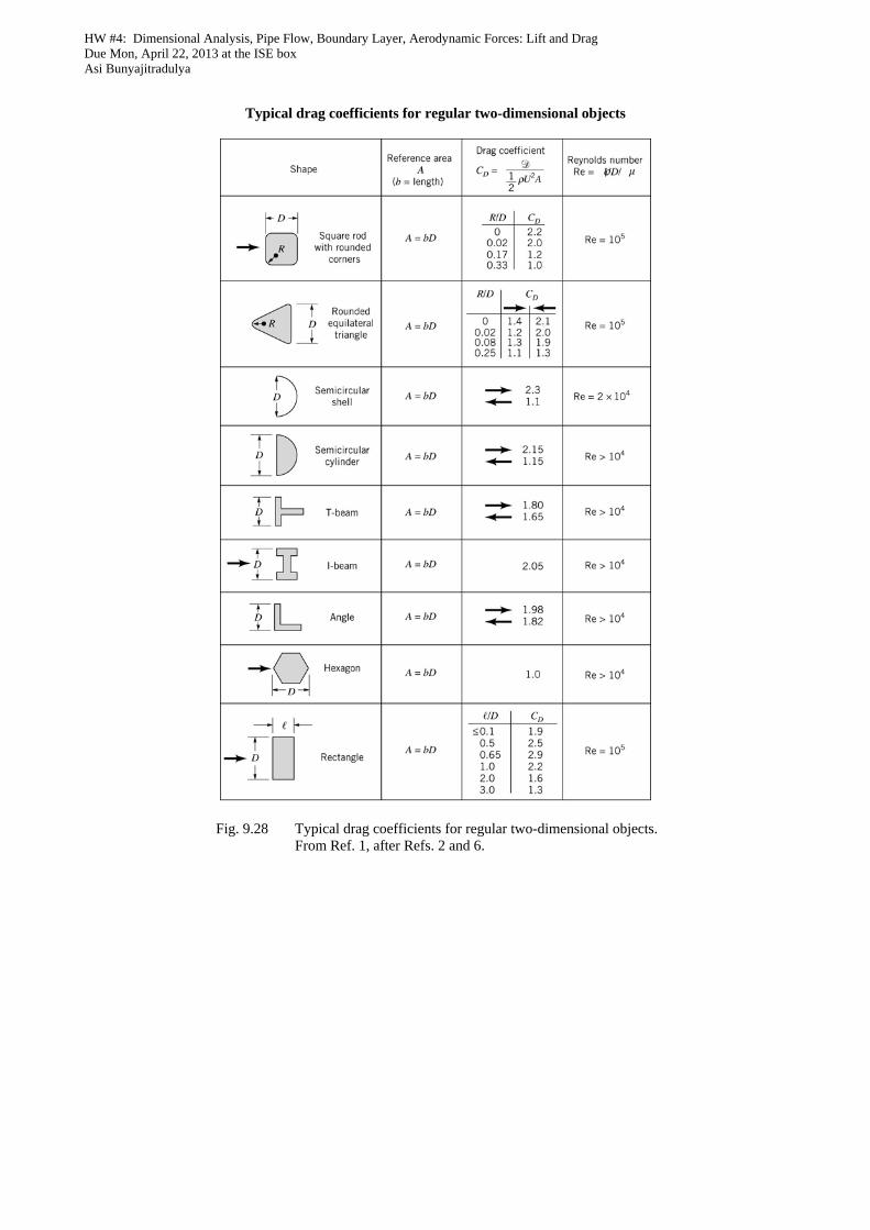
Typical drag coefficients for regular two-dimensional objects

Fig. 9.28 Typical drag coefficients for regular two-dimensional objects. From Ref. 1, after Refs. 2 and 6.


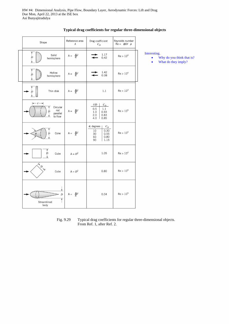
Typical drag coefficients for regular three-dimensional objects

Fig. 9.29 Typical drag coefficients for regular three-dimensional objects.

From Ref. 1, after Ref. 2.

Interesting. Why do you think that is? What do they imply?


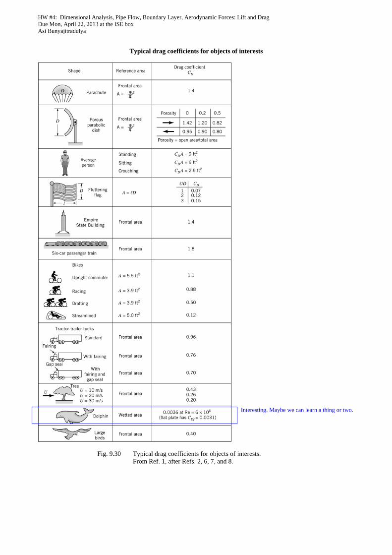
Typical drag coefficients for objects of interests

Fig. 9.30 Typical drag coefficients for objects of interests.

From Ref. 1, after Refs. 2, 6, 7, and 8.

Interesting. Maybe we can learn a thing or two.


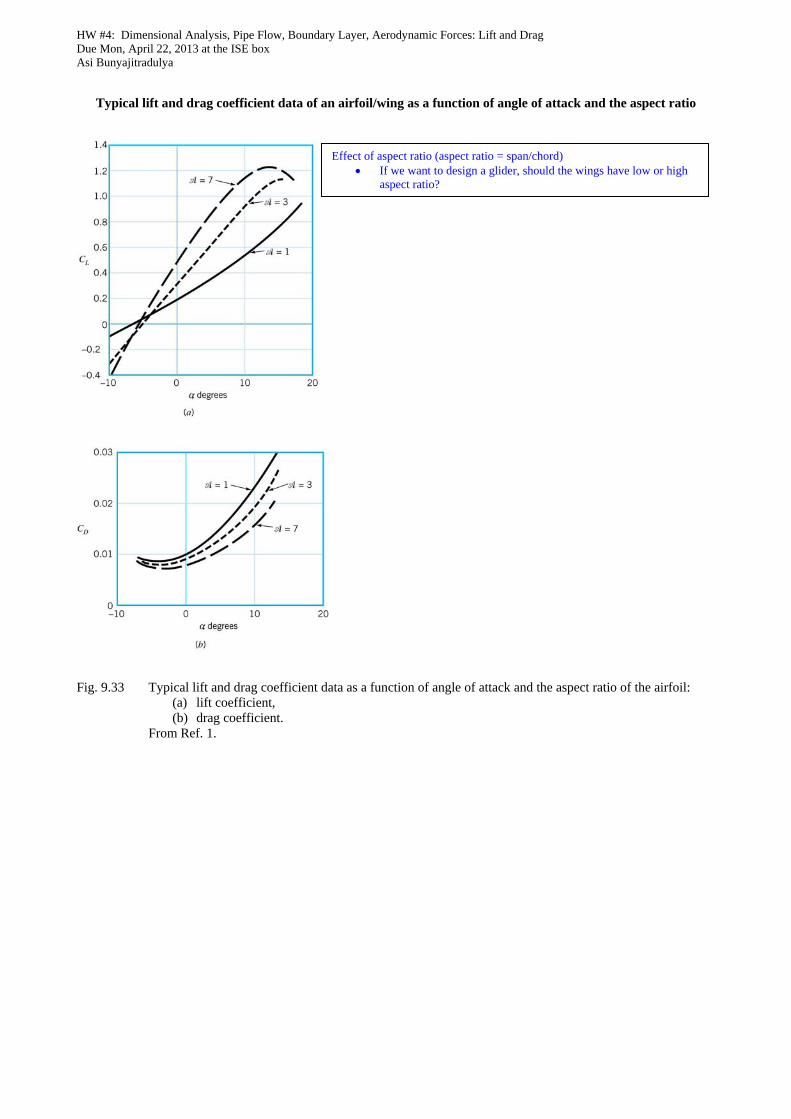
Typical lift and drag coefficient data of an airfoil/wing as a function of angle of attack and the aspect ratio

Fig. 9.33 Typical lift and drag coefficient data as a function of angle of attack and the aspect ratio of the airfoil:

(a) lift coefficient, (b) drag coefficient.

From Ref. 1.

Effect of aspect ratio (aspect ratio = span/chord) If we want to design a glider, should the wings have low or high

aspect ratio?


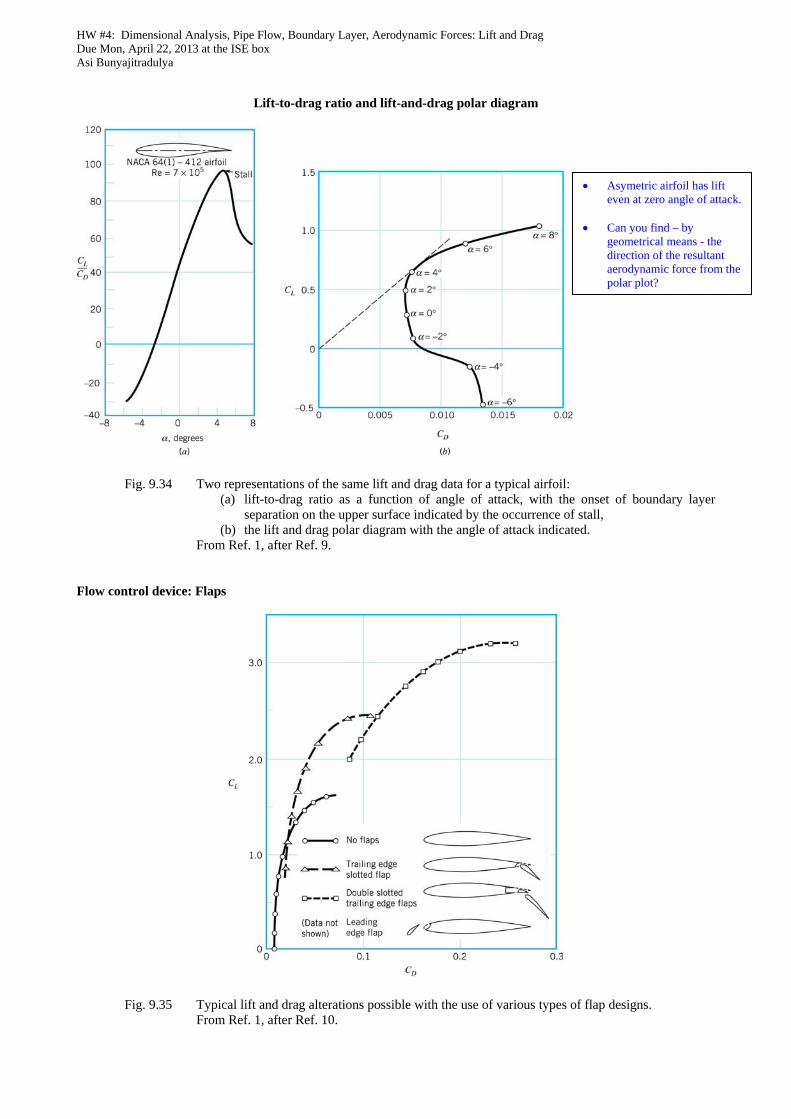
Lift-to-drag ratio and lift-and-drag polar diagram

Fig. 9.34 Two representations of the same lift and drag data for a typical airfoil:

(a) lift-to-drag ratio as a function of angle of attack, with the onset of boundary layer separation on the upper surface indicated by the occurrence of stall,

(b) the lift and drag polar diagram with the angle of attack indicated. From Ref. 1, after Ref. 9.

Flow control device: Flaps

Fig. 9.35 Typical lift and drag alterations possible with the use of various types of flap designs.

From Ref. 1, after Ref. 10.

Asymetric airfoil has lift even at zero angle of attack.

Can you find – by

geometrical means - the direction of the resultant aerodynamic force from the polar plot?


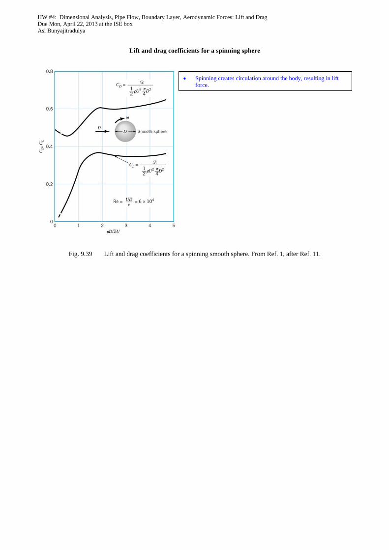
Lift and drag coefficients for a spinning sphere

Fig. 9.39 Lift and drag coefficients for a spinning smooth sphere. From Ref. 1, after Ref. 11.

Spinning creates circulation around the body, resulting in lift force.

Documents

HW #4: Dimensional Analysis, Pipe Flow, Boundary Layer ...fmeabj.lecturer.eng.chula.ac.th/2142-242 HP/242 Course Materials... · Munson B. R., Young, D. F., and Okiishi, T. H., 2002,