HW 2, Part 1

Question 1 (In EXCEL)

Create a data set with the following characteristics:

Sample size: 100

One independent variable: x, with a range of 1- 50 (You can use the ‘randbetween’ command on

excel)

One response variable: y , Let y = 3 + 3e.02x

A) Create a scatter plot of y as a function of x in EXCEL, and save the plot in a word document.

B) Use EXCEL to perform a linear regression, 2nd order polynomial regression, and an exponential

regression. On the same word document where you have your plot, record the equations and the R2

values for each regression.

C) Try to explain the trends in regression coefficients. Why does the polynomial regression fit better than

the exponential regression, even though the data set was created with an exponential function? Will a

polynomial regression fit any data set at least as well as a linear regression? Why?

Exponential gives better fit (higher R2) value than linear, as it is curved and fits better than a line.

Polynomial is a nonlinear model but has three parameters rather than two parameters in the exponential

and linear. More parameters usually leads to a better fit.

D) If you have some data and want to perform a regression, what will be your criteria for selecting the

appropriate type of regression?

Usually we use sum squared error or R2 value to determine goodness of fit.

HW 2, Part 2

1. Open your BMEN 211 folder in a file browser window.

2. Right click in your folder and select “New” then select “Microsoft Excel Worksheet”

3. Rename this worksheet “BMEN211Lab1-2011” and open the Excel document.

4. In “Sheet1” put the following values in Columns B and C, rows 1 to 9:

5. These values are for the initial time, final time, time step size, the size of the input flow change, the initial tank

height, the valve coefficient, and the tank area. These must be in the exact positions as above, columns B and C

rows 1 to 7.

6. Click the “View” tab at the top.

7. Find the “Macro” button on the far right.

8. Click the “Macro Arrow” button (not the icon) then select “Record Macro” and enter the macro name

“RunSimulation” and give your macro a shortcut, CTRL-t.

9. Immediately, click the “Macro Arrow” button (not the icon) and select “Record Macro” and click “Stop

Recording.” This is important.

10. Click the Macro Icon to open a list of macros. Select your macro from the list (RunSimulation) then hit edit. This

should open the VBA editing environment. You can switch back to excel using Alt-Tab.

11. The VBA editing environment looks like this: Note that

anything on a line after a single quote is treated as a comment and should appear in green.

12. Put the code below (in the CODE SECTION) into your VBA macro and save your file. Put your name in the title

section! This should be a bit of typing exercise. Be very careful when copying. Also, note that the code goes

below the green header comments and above the End Sub line (which ends the subroutine declaration)

13. Look at the code. Notice the For statement and If statement.

14. On the “File” tab select “Save As” and choose “Excel Macro-Enabled Workbook”.

15. Run your simulation by hitting Ctrl-t and you should get some data. Make a figure like the following using a

scatter plot for T, U, H.

16. Put your figure in a Word Doc to print out later. YOU SHOULD PASTE INTO WORD AS “PASTE SPECIAL,

PICTURE” Otherwise any change in the excel document will change the figure in your Word doc.

17. Increase the value for k by .5 and run the simulation. Keep increasing k and running the simulation until the

simulation “breaks.” This happens when the simulation tries to take a square root of a negative number.

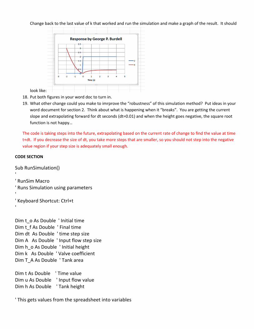
Change back to the last value of k that worked and run the simulation and make a graph of the result. It should

look like:

18. Put both figures in your word doc to turn in.

19. What other change could you make to imrprove the “robustness” of this simulation method? Put ideas in your

word document for section 2. Think about what is happening when it “breaks”. You are getting the current

slope and extrapolating forward for dt seconds (dt=0.01) and when the height goes negative, the square root

function is not happy…

The code is taking steps into the future, extrapolating based on the current rate of change to find the value at time

t+dt. If you decrease the size of dt, you take more steps that are smaller, so you should not step into the negative

value region if your step size is adequately small enough.

CODE SECTION

Sub RunSimulation()

'

' RunSim Macro

' Runs Simulation using parameters

'

' Keyboard Shortcut: Ctrl+t

'

Dim t_o As Double ' Initial time

Dim t_f As Double ' Final time

Dim dt As Double ' time step size

Dim A As Double ' Input flow step size

Dim h_o As Double ' Initial height

Dim k As Double ' Valve coefficient

Dim T_A As Double ' Tank area

Dim t As Double ' Time value

Dim u As Double ' Input flow value

Dim h As Double ' Tank height

' This gets values from the spreadsheet into variables

t_o = Range("C1")

t_f = Range("C2")

dt = Range("C3")

A = Range("C4")

h_o = Range("C5")

k = Range("C6")

T_A = Range("C7")

' This sets up where the data will go and deletes the old stuff

Range("F9") = "T"

Range("G9") = "U"

Range("H9") = "H"

Range("F10:H3000").Delete

Range("F10").Select

' Set t and h to their initial values

t = t_o

h = h_o

' This is a FOR loop, when you know how many times to run

For i = 1 To 1 + ((t_f - t_o) / dt)

' This is an IF statement, conditional execution

If (t < 0) Then ' This sets the u value for right now

u = 0

Else

u = A

End If

' This writes the values into the spreadsheet

Cells(i + 9, "F") = t

Cells(i + 9, "G") = u

Cells(i + 9, "H") = h

' This updates t and h for the next iteration

t = t + dt

h = h + dt * (u - k * Sqr(h)) / T_A

Next i ' This is the end of the For loop

' Note the indentation levels above. This helps read code!

End Sub

HW 2, Part 3

1. A process is to be modeled inside a cell. It is theorized that species B diffuses into a cell. It then

diffuses into the nucleus where it reacts to form species C. C does not leave the nucleus or react in

any way, it accumulates continuously increasing amounts. Assume the following:

Molar diffusion rate of B into the cell is D1A1(CBo(t)-CB(t))

Molar diffusion rate of B into the nucleus is D2A2(CB(t)-CBn(t))

Volume of cell outside the nucleus is V

Effective volume of cell in nucleus is Vn

Reaction rate of B changing to C is VnkCBn(t)

Develop a dynamic model for this system.

V dCb/dt = D1A1(CBo(t)-CB(t)) - D2A2(CB(t)-CBn(t))

Vn dCbn/dt = D2A2(CB(t)-CBn(t)) - VnkCBn(t)

Vn dCc/dt = VnkCBn(t)

2. For the following data: x y

100 5.5

200 7.8

300 9.5

400 13.2

Find the following approximate values:

y=f(x=170)

y=f(x=390)

y=f(x=25)

y=f(x=500)

The formula is f(x)=f(x0) + m (x-x0) with m = ( f(x1)-f(x0) ) / (x1-x0)

y=f(x=170) = f(100) + ( 170 – 100 ) * ( f(200)-f(100) ) / (200-100) = 7.11

y=f(x=390) = f(300) + ( 390 – 300 ) * ( f(400)-f(300) ) / (400-300) = 12.83

y=f(x=25) = f(100) + ( 25 – 100 ) * ( f(200)-f(100) ) / (200-100) = 3.775

y=f(x=500) = f(400) + ( 500 – 400 ) * ( f(400)-f(300) ) / (400-300) = 16.9

3. Total drug in for a second order system response can be given as:

y(x)=exp(-2x)-exp(x)

Approximate the integral of y(x) using the trapezoidal rule from x=0 to x=5 with N=5.

Knowing that the area of a trapezoid is (a+b) h /2, with h=1 the total for the five trapezoids based on

the data below is -158.7

y(x)=exp(-2x)-exp(x)

x F(x)

0 0

1 -2.58295

2 -7.37074

3 -20.0831

4 -54.5978

5 -148.413

(1/2)*( 0 + 2* (-2.582+ -7.37 + -20.0 + -54.59 ) + -148.4 ) = -158.7

Or just adding up 5 individual trapezoid areas:

(0+-2.5)*1/2+(-2.58+-7.37)*1/2+(-7.37+-20.08)*1/2+(-20.08+-54.59)*1/2+(-54.59+-148.4)*1/2=-158.7

Wolfram Alpha says the true value is -146.9

++= ∑−

=

)()(2)(2

1

10 N

N

iiT xfxfxf

hI

HW 2, Part 4

Open excel. Make a data set with 18 data points with reaction rate R as a function of concentration C. The

concentration values should be between 1 and 10 (use randbetween(1,10) and the reaction rate should be the

following expression: 5*Conc/(3+Conc)+(RAND()-0.5) This reaction rate expression represents Michaelis-Menten

kinetics in the form: ���� ������

���� with some additional noise on the rate measurement value.

Every time you make a change in excel, the random functions change values. Take a “snapshot” of your data

by copying/pasting (paste special values) into two locations, columns E&F and columns H &I. In location M2

and M3 put the text Vmax and Km. In location N2 and N3 put the values 5 and 3. In column J, develop model

equations for the modeled rate that depend on the concentration and the values for Vmax and Km in location

N2 and N3. N2 and N3 must be “anchored” using $N$2 and $N$3. In column K, develop equations for the

difference between the measure rate and the model rate, squared (use parenthesis around the values then

^2). Use the sum command to find the sum of the errors squared. Put the sum of all the error squared values

in cell K22, the sum of that column (use =sum(K3:K20) in cell K22). Your spreadsheet my look like:

Now, select your first set of data (E2:F20). Select Home->Sort & Filter ->Sort Smallest to Largest. Repeat for

Columns H and I. Next, try a custom sort. Select (E2:F20) and use Home->Sort & Filter -> Custom Sort. Add a

level and have it sort by rate after it sorts by concentration.

Nonlinear optimization using Solver. Select File-> Options. Select Add-Ins from the left tab list. Select “Solver

Add-In” and hit the “Go” button (Not OK). Select the solver check box and hit ok.

In Data->Solver set the wizard to have Objective function $K$22, set the minimize radio button, and have it change cells

$N$2:$N$3. Hit the solve button, then accept the answer. Make the scatter plot for your data and model for your word

document. Change the line types so that the data is not connected but the model is. What are your resulting values for

Vmax and Km. Do the resulting values for Vmax and Km match your “true” values? Why or why not.

The data includes some random noise. The best fit line through the data will probably not match the true values

because it is likely with a small number of data points that more of the data will be a bit high or a bit low. Given many

more data points, eventually it is likely that the average best fit would match the true values.

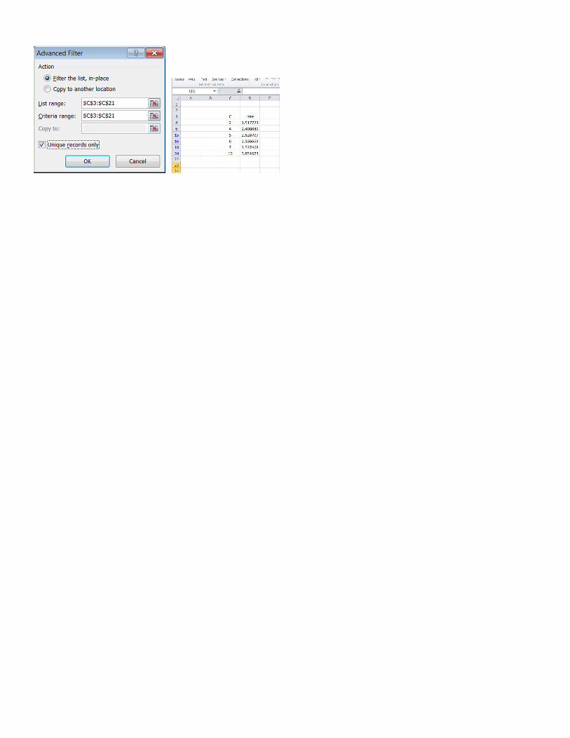
Removal of duplicates. Copy your data set into a different sheet (sheet2). Select Data->Filter-Advanced. Select only the

column for C for both list and criteria range. Hit ok. This hides rows where C was evaluated multiple times. Note you

can undo this under Data->Filter clear. Make a screen capture of your sheet (alt-PrScr) and paste it into your Word doc.

Double click the image and select the crop tool to only show the portion like below.