Embed Size (px)
Citation preview
HVAC Instrumentation and Controls Course No: M06-019
Credit: 6 PDH
A. Bhatia
Continuing Education and Development, Inc. 9 Greyridge Farm Court Stony Point, NY 10980 P: (877) 322-5800 F: (877) 322-4774 [email protected]
HVAC Instrumentation and Control
The application of Heating, Ventilating, and Air-Conditioning (HVAC) controls starts with
an understanding of the building and the use of the spaces to be conditioned and
controlled. All control systems operate in accordance with few basic principles but before
we discuss these, let’s address few fundamentals of the HVAC system first.
Why Automatic Controls?
The capacity of the HVAC system is typically designed for the extreme conditions. Most
operation is part load/off design as variables such as solar loads, occupancy, ambient
temperatures, equipment & lighting loads etc keep on changing through out the day.
Deviation from design will result in drastic swings or imbalance since design capacity is
greater than the actual load in most operating scenarios. Without control system, the
system will become unstable and HVAC would overheat or overcool spaces.
HVAC systems
HVAC systems are classified as either self-contained unit packages or as central systems.
A unit package describes a single unit that converts a primary energy source (electricity or
gas) and provides final heating and cooling to the space to be conditioned. Examples of
self-contained unit packages are rooftop HVAC systems, air conditioning units for rooms,
and air-to-air heat pumps.
With central systems, the primary conversion from fuel such as gas or electricity takes
place in a central location, with some form of thermal energy distributed throughout the
building or facility.
Central systems are a combination of central supply subsystem and multiple end use
subsystems. There are many variations of combined central supply and end use zone
systems. The most frequently used combination is central hot and chilled water distributed
to multiple fan systems. The fan systems use water-to-air heat exchangers called coils to
provide hot and/or cold air for the controlled spaces. End-use subsystems can be fan
systems or terminal units. If the end use subsystems are fan systems, they can be single
or multiple zone type. The multiple end use zone systems are mixing boxes, usually called
VAV boxes.
Another combination central supply and end use zone system is a central chiller and boiler
system for the conversion of primary energy, as well as a central fan system to delivery
hot and/or cold air. The typical uses of central systems are in larger, multistory buildings
where access to outside air is more restricted. Typically central systems have lower
operating costs but have a complex control sequence.
How does central air-conditioning system work?
Cooling Cycle (chilled water system): The supply air, which is approximately 20° F
cooler than the air in the conditioned space, leaves the cooling coil through the supply air
fan, down to the ductwork and into the conditioned space. The cool supply air picks up
heat in the conditioned space and the warmer air makes its way into the return air duct
back to the air handling unit. The return air mixes with outside air in a mixing chamber and
goes through the filters and cooling coil. The mixed air gives up its heat into the chilled
water tubes in the cooling coil, which has fins attached to the tubes to facilitate heat
transfer. The cooled supply air leaves the cooling coil and the air cycle repeats.
The chilled water circulating through the cooling coil tubes, after picking up heat from the
mixed air, leaves the cooling coil and goes through the chilled water return (CHWR) pipe
to the chiller's evaporator. Here it gives up the heat into the refrigeration system. The
newly "chilled" water leaves the evaporator and is pumped through the chilled water
supply (CHWS) piping into the cooling coil continuously and the water cycle repeats.
The evaporator is a heat exchanger that allows heat from the CHWR to flow by conduction
into the refrigerant tubes. The liquid refrigerant in the tubes "boils off" to a vapor removing
heat from the water and conveying the heat to the compressor and then to the condenser.
The heat from the condenser is conveyed to the cooling tower by the condenser water.
Finally, outside air is drawn across the cooling tower, removing the heat from the water
through the process of evaporation.
The figure below provides a conceptual view of a chilled water air-conditioning system with
water-cooled condenser.
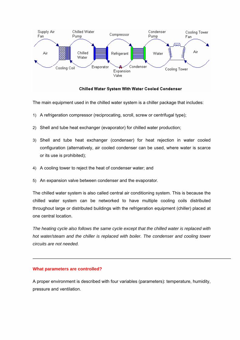
The main equipment used in the chilled water system is a chiller package that includes:
1) A refrigeration compressor (reciprocating, scroll, screw or centrifugal type);
2) Shell and tube heat exchanger (evaporator) for chilled water production;
3) Shell and tube heat exchanger (condenser) for heat rejection in water cooled
configuration (alternatively, air cooled condenser can be used, where water is scarce
or its use is prohibited);
4) A cooling tower to reject the heat of condenser water; and
5) An expansion valve between condenser and the evaporator.
The chilled water system is also called central air conditioning system. This is because the
chilled water system can be networked to have multiple cooling coils distributed
throughout large or distributed buildings with the refrigeration equipment (chiller) placed at
one central location.
The heating cycle also follows the same cycle except that the chilled water is replaced with
hot water/steam and the chiller is replaced with boiler. The condenser and cooling tower
circuits are not needed.
What parameters are controlled?
A proper environment is described with four variables (parameters): temperature, humidity,
pressure and ventilation.
Temperature
The comfort zone for temperature is between 68°F (20°C) and 75°F (25°C). Temperatures
less than 68°F (20°C) may cause some people to feel too cool. Temperatures greater than
78°F (25°C) may cause some people to feel too warm.
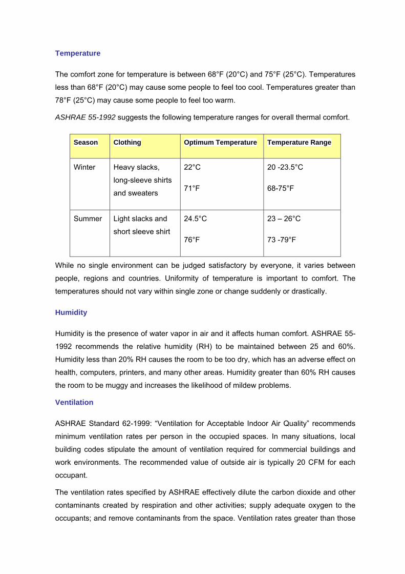
ASHRAE 55-1992 suggests the following temperature ranges for overall thermal comfort.
Season Clothing Optimum Temperature Temperature Range
Winter Heavy slacks,
long-sleeve shirts
and sweaters
22°C
71°F
20 -23.5°C
68-75°F
Summer Light slacks and
short sleeve shirt
24.5°C
76°F
23 – 26°C
73 -79°F
While no single environment can be judged satisfactory by everyone, it varies between
people, regions and countries. Uniformity of temperature is important to comfort. The
temperatures should not vary within single zone or change suddenly or drastically.
Humidity
Humidity is the presence of water vapor in air and it affects human comfort. ASHRAE 55-
1992 recommends the relative humidity (RH) to be maintained between 25 and 60%.
Humidity less than 20% RH causes the room to be too dry, which has an adverse effect on
health, computers, printers, and many other areas. Humidity greater than 60% RH causes
the room to be muggy and increases the likelihood of mildew problems.
Ventilation
ASHRAE Standard 62-1999: “Ventilation for Acceptable Indoor Air Quality” recommends
minimum ventilation rates per person in the occupied spaces. In many situations, local
building codes stipulate the amount of ventilation required for commercial buildings and
work environments. The recommended value of outside air is typically 20 CFM for each
occupant.
The ventilation rates specified by ASHRAE effectively dilute the carbon dioxide and other
contaminants created by respiration and other activities; supply adequate oxygen to the
occupants; and remove contaminants from the space. Ventilation rates greater than those
recommended by ASHARE criteria are sometimes required for controlling odors and
where cooling is not provided to offset heat gains.
Pressure
Air moves from areas of higher pressure to areas of lower pressure through any available
opening. A small crack or hole can admit significant amounts of air, if the pressure
differentials are high enough (which may be very difficult to assess). The rooms and
buildings typically have a slightly positive pressure to reduce outside air infiltration. This
helps in keeping the building clean. Typically the stable positive pressure of .01-.05” is
recommended. Pressure is an issue that comes into play in buildings where air quality is
strictly monitored; for example hospitals.
Special Control Requirements
The special requirements pertain to the interlocking with fire protection systems, smoke
removal systems, clean air systems, hazardous or noxious effluent control, etc.
Control Strategies
The simplest control in HVAC system is cycling or on/off control to meet part load
conditions. If building only needs half the energy that the system is designed to deliver, the
system runs for about ten minutes, turns off for ten minutes, and then cycles on again. As
the building load increases, the system runs longer and its off period is shorter.
One problem faced by this type of control is short-cycling which keeps the system
operating at the inefficient condition and wears the component quickly. A furnace or air-
conditioner takes several minutes before reaching "steady-state" performance.
Lengthening the time between starts to avoid short-cycling is possible but at the cost of
some discomfort for a short time.
The longer the time between cycles, the wider the temperature swings in the space. Trying
to find a compromise that allows adequate comfort without excessive wear on the
equipment is modulation or proportional control. Under this concept, if a building is calling
for half the rated capacity of the chiller, the chilled water is supplied at half the rate or in
case of a heating furnace; fuel is fed to the furnace at half the design rate (the energy
delivery is proportional to the energy demand). While this system is better than cycling, it
also has its problems. Equipment has a limited turn-down ratio. A furnace with a 5:1 turn-
down ratio can only be operated above 20% of rated capacity. If the building demand is
lower than that, cycling would still have to be used.
An alternate method of control under part-load conditions is staging. Several small units
(e.g., four units at 25% each) are installed instead of one large unit. When conditions call
for half the design capacity, only two units operate. At 60% load, two units are base-
loaded (run continuously), and a third unit swings (is either cycled or modulated) as
needed. To prevent excessive wear, sequencing is often used to periodically change the
unit being cycled. To continue our example at 60% load: assume Units 1 and 2 are base-
loaded, and Unit 3 has just cycled on. When the cycling portion of the load is satisfied, Unit
1 cycles off, and Units 2 and 3 become base loaded. When more capacity is needed, Unit
4 cycles on, and so on.
Where are HVAC controls required?
The HVAC control system is typically distributed across three areas:
1) The HVAC equipment and their controls located in the main mechanical room.
Equipment includes chillers, boiler, hot water generator, heat exchangers, pumps, etc.
2) The weather maker or the “Air Handling Units (AHUs)” may heat, cool, humidify,
dehumidify, ventilate, or filter the air and then distribute that air to a section of the
building. AHUs are available in various configurations and can be placed in a
dedicated room called secondary equipment room or may be located in an open area
such as roof top air-handling units.
3) The individual room controls depending on the HVAC system design. The equipment
includes fan coil units, variable air volume systems, terminal reheat, unit ventilators,
exhausters, zone temperature/humidistat devices, etc.
Benefits of a Control System
Controls are required for one or more of the following reasons:
1) Maintain thermal comfort conditions
2) Maintain optimum indoor air quality
3) Reduce energy use
4) Safe plant operation
5) To reduce manpower costs
6) Identify maintenance problems
7) Efficient plant operation to match the load
8) Monitoring system performance
Control Basics
What is Control?
In simplest terms, the control is defined as the starting, stopping or regulation of heating,
ventilating, and air conditioning system. Controlling an HVAC system involves three
distinct steps:
1) Measure a variable and collect data
2) Process the data with other information
3) Cause a control action
The above three functions are met through sensor, controller and the controlled device.
Elements of a Control System
HVAC control system, from the simplest room thermostat to the most complicated
computerized control, has four basic elements: sensor, controller, controlled device and
source of energy.
1) Sensor measures actual value of controlled variable such as temperature, humidity or
flow and provides information to the controller.
2) Controller receives input from sensor, processes the input and then produces
intelligent output signal for controlled device.
3) Controlled device acts to modify controlled variable as directed by controller.
4) Source of energy is needed to power the control system. Control systems use either a
pneumatic or electric power supply.
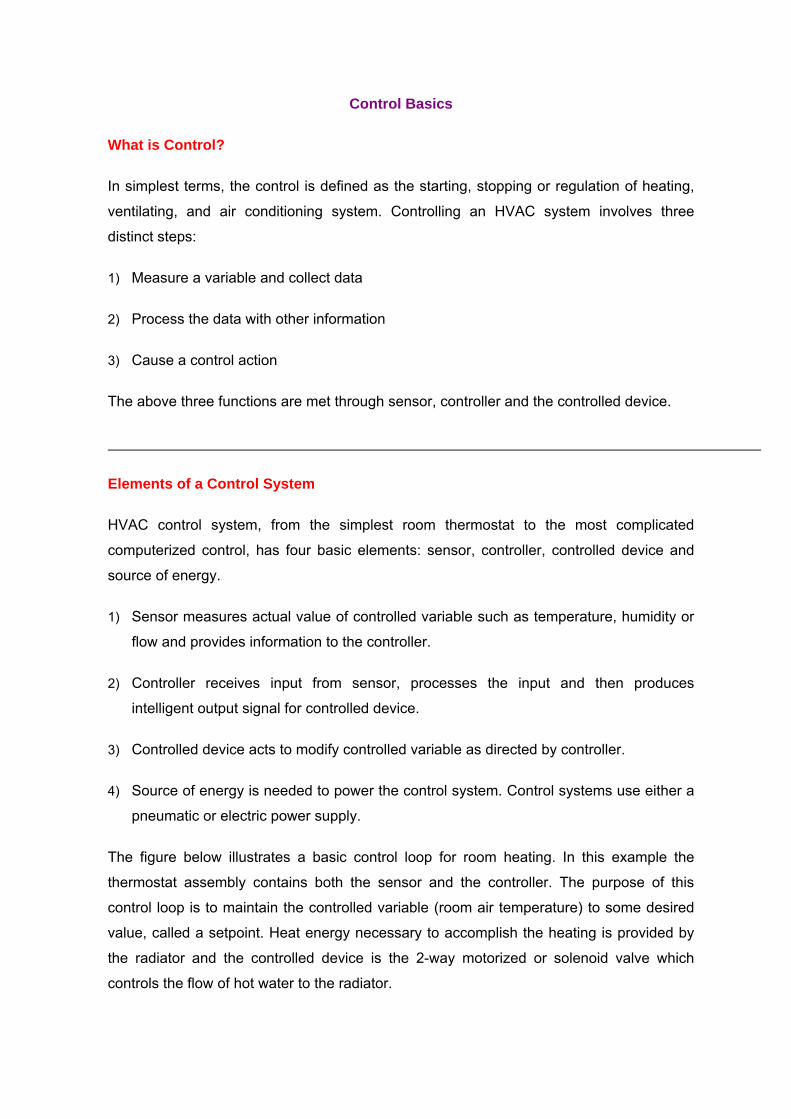
The figure below illustrates a basic control loop for room heating. In this example the
thermostat assembly contains both the sensor and the controller. The purpose of this
control loop is to maintain the controlled variable (room air temperature) to some desired
value, called a setpoint. Heat energy necessary to accomplish the heating is provided by
the radiator and the controlled device is the 2-way motorized or solenoid valve which
controls the flow of hot water to the radiator.
Theory of Controls
Basically there are two types of controls: open loop control and closed loop control.
Open loop control
Open loop control is a system with no feedback; i.e. there is no way to monitor if the
control system is working effectively. Open loop control is also called feed forward control.
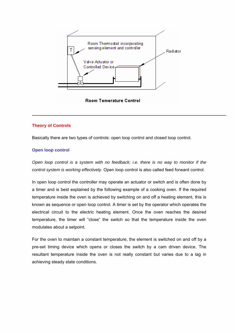
In open loop control the controller may operate an actuator or switch and is often done by
a timer and is best explained by the following example of a cooking oven. If the required
temperature inside the oven is achieved by switching on and off a heating element, this is
known as sequence or open loop control. A timer is set by the operator which operates the
electrical circuit to the electric heating element. Once the oven reaches the desired
temperature, the timer will “close” the switch so that the temperature inside the oven
modulates about a setpoint.
For the oven to maintain a constant temperature, the element is switched on and off by a
pre-set timing device which opens or closes the switch by a cam driven device. The
resultant temperature inside the oven is not really constant but varies due to a lag in
achieving steady state conditions.
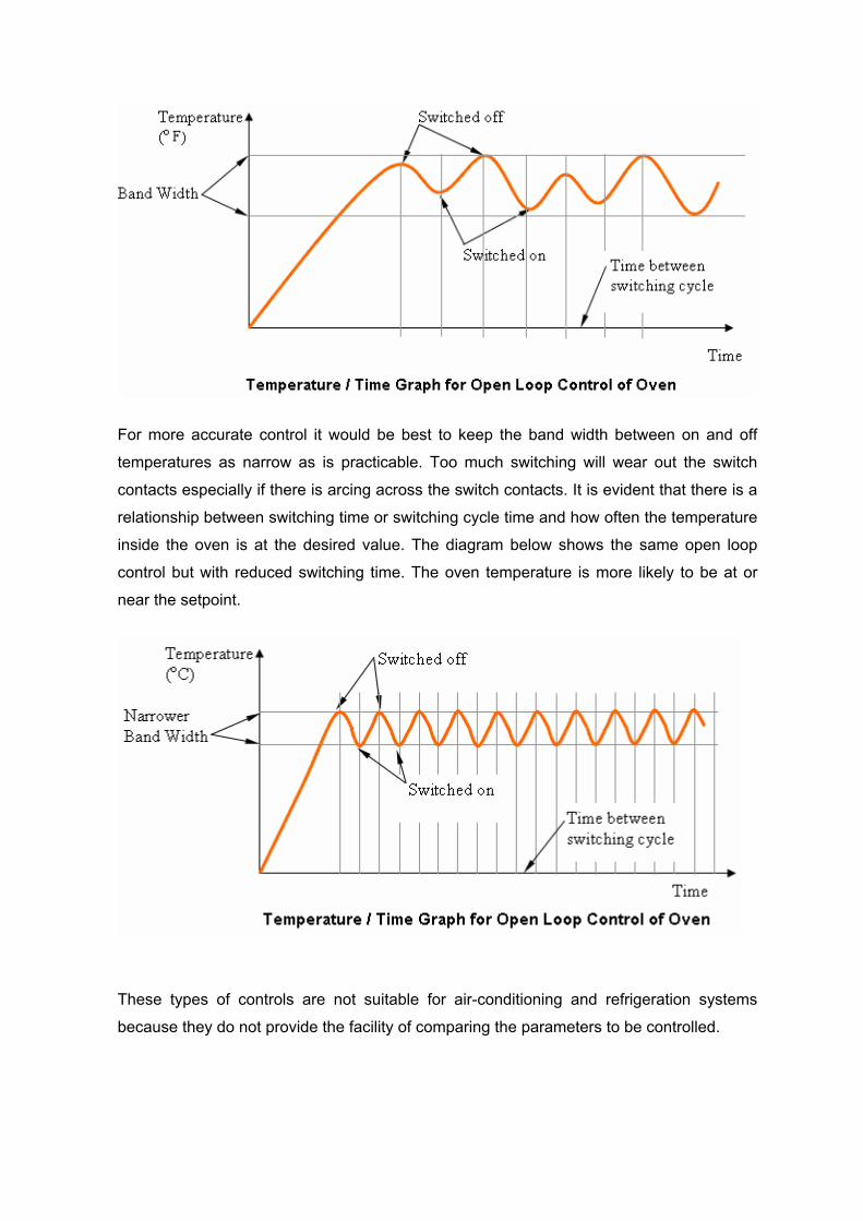
For more accurate control it would be best to keep the band width between on and off
temperatures as narrow as is practicable. Too much switching will wear out the switch
contacts especially if there is arcing across the switch contacts. It is evident that there is a
relationship between switching time or switching cycle time and how often the temperature
inside the oven is at the desired value. The diagram below shows the same open loop
control but with reduced switching time. The oven temperature is more likely to be at or
near the setpoint.
These types of controls are not suitable for air-conditioning and refrigeration systems
because they do not provide the facility of comparing the parameters to be controlled.
Closed Loop System
If the oven in the example had a temperature measuring device and the temperature
inside was continually being compared with the desired temperature then this information
could be used to adjust the amount of heat input to the electric element. In the closed
system, the controller responds to error in controlled variable. A comparison of the sensed
parameters is made with respect to the set parameters and accordingly the corresponding
signals will be generated. Closed loop control is also called feedback control.
In general, if the sensor measures a controlled variable, then the control system is closed
loop; if not, then the system is open loop.
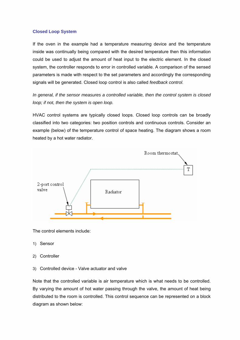
HVAC control systems are typically closed loops. Closed loop controls can be broadly
classified into two categories: two position controls and continuous controls. Consider an
example (below) of the temperature control of space heating. The diagram shows a room
heated by a hot water radiator.
The control elements include:
1) Sensor
2) Controller
3) Controlled device - Valve actuator and valve
Note that the controlled variable is air temperature which is what needs to be controlled.
By varying the amount of hot water passing through the valve, the amount of heat being
distributed to the room is controlled. This control sequence can be represented on a block
diagram as shown below:
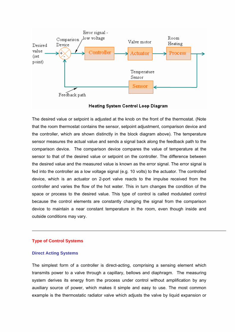
The desired value or setpoint is adjusted at the knob on the front of the thermostat. (Note
that the room thermostat contains the sensor, setpoint adjustment, comparison device and
the controller, which are shown distinctly in the block diagram above). The temperature
sensor measures the actual value and sends a signal back along the feedback path to the
comparison device. The comparison device compares the value of temperature at the
sensor to that of the desired value or setpoint on the controller. The difference between
the desired value and the measured value is known as the error signal. The error signal is
fed into the controller as a low voltage signal (e.g. 10 volts) to the actuator. The controlled
device, which is an actuator on 2-port valve reacts to the impulse received from the
controller and varies the flow of the hot water. This in turn changes the condition of the
space or process to the desired value. This type of control is called modulated control
because the control elements are constantly changing the signal from the comparison
device to maintain a near constant temperature in the room, even though inside and
outside conditions may vary.
Type of Control Systems
Direct Acting Systems
The simplest form of a controller is direct-acting, comprising a sensing element which
transmits power to a valve through a capillary, bellows and diaphragm. The measuring
system derives its energy from the process under control without amplification by any
auxiliary source of power, which makes it simple and easy to use. The most common
example is the thermostatic radiator valve which adjusts the valve by liquid expansion or
vapor pressure. Direct-acting thermostats have little power and some disadvantages but
the main advantage is individual and inexpensive emitter control. Direct-acting thermo-
static equipment gives gradual movement of the controlling device and may modulate.
Electric / Electronic Systems
Electric controlled devices provide ON/OFF or two-position control. In residential and small
commercial applications, low voltage electrical controls are most common. A transformer
is used to reduce the 115 volt alternating current (AC) to a nominal 24 volts. This voltage
signal is controlled by thermostats, and can open gas solenoid valves, energize oil burners
or solenoid valves on the DX cooling, control electric heat, operate two position valves and
dampers, or turn on-off fans and pumps. A relay or contactor is used to switch line voltage
equipment with the low voltage control signal. The advantage of an electric system is that
it eliminates the personnel safety and fire risk associated with line voltage, and allows
these control wires to be installed by a non-electrician without requiring conduit and other
safety measures. However, these systems are generally limited to providing on/off control
only: they cannot operate at half capacity.
Electronic Controlled Devices can be either modulating or two-position (ON/OFF).
Electronic control systems usually have the following characteristics:
1) Controller: Low voltage, solid state
2) Inputs: 0 to 1V dc, 0 to 10V dc, 4 to 20 mA, resistance element, thermistor, and
thermocouple
3) Outputs: 2 to 10V dc or 4 to 20 mA device
4) Control Mode: Two-position, proportional or proportional plus integral (PI)
Other features of electronic control systems include:
1) Controllers can be remotely located from sensors and actuators.
2) Controllers can accept a variety of inputs.
3) Remote adjustments for multiple controls can be located together, even though
sensors and actuators are not.
4) Electronic control systems can accommodate complex control and override schemes.
5) Universal type outputs can interface many different actuators.
6) Display meters indicate input or output values.
An electronic control system can be enhanced with visual displays that show system
status and operation. Many electronic controllers have built-in indicators that show power,
input signal, deviation signal, and output signal. An indicator light can show on/off status
or, if driven by controller circuits, the brightness of a light can show the relative strength of
a signal.
Pneumatic Systems
Historically, the most popular control system for large buildings has been a pneumatic
system which can provide both on/off and modulating control. Pneumatic actuators are
described in terms of their spring range. Common spring ranges are 3 to 8 psig (21 to 56
kPa), 5 to 10 psig (35 to 70 kPa), and 8 to 13 psig (56 to 91 kPa).
Compressed air with an input pressure can be regulated by thermostats and humidistat.
By varying the discharge air pressure from these devices, the signal can be used directly
to open valves, close dampers, and energize other equipment. The copper or plastic
tubing carries the control signals around the building, which is relatively inexpensive. The
pneumatic system is very durable, safe in hazardous areas where electrical sparks must
be avoided, and most importantly, capable of modulation or operation at part load
condition. While the 24 volt electrical control system could only energize a damper fully
open or fully closed, a pneumatic control system can hold that damper at 25%, 40% or
80% open. This allows more accurate matching of the supply with the load.
Pneumatic controls use clean, dry and oil free compressed air, both as the control signal
medium and to drive the valve stem with the use of diaphragms. It is important that dirt,
moisture and oil are absent from the compressed air supply. Instrument quality of
compressed air is more suitable for controls rather than industrial quality and requires
drying to a dew-point low enough to satisfy the application. The main disadvantages are
less reliability and more noise when compared to electronic systems.
Microprocessor Systems
Direct Digital Control (DDC) is the most common deployed control system today. The
sensors and output devices (e.g., actuators, relays) used for electronic control systems are
usually the same ones used on microprocessor-based systems. The distinction between
electronic control systems and microprocessor-based systems is in the handling of the
input signals. In an electronic control system, the analog sensor signal is amplified, and
then compared to a setpoint or override signal through voltage or current comparison and
control circuits. In a microprocessor-based system, the sensor input is converted to a
digital form, where discrete instructions (algorithms) perform the process of comparison
and control. Most subsystems, from VAV boxes to boilers and chillers, now have a built-in
DDC system to optimize the performance of that unit. A communication protocol known as
BACNet is a standard protocol that allows control units from different manufacturers to
pass data to each other.
Mixed Systems
Combinations of controlled devices are possible. For example, electronic controllers can
modulate a pneumatic actuator. Also, proportional electronic signals can be sent to a
device called transducer which converts these signals into proportional air pressure
signals used by the pneumatic actuators. These are known as electronic-to-pneumatic
(E/P) transducers. For example, an E/P transducer converts a modulating 2 to 10V dc
signal from the electronic controller to a pneumatic proportional modulating 3 to 13 psi
signal for a pneumatic actuator. A sensor-transducer assembly is called a transmitter.
The input circuits for many electronic controllers can accept a voltage range of 0 to 10V dc
or a current range of 4 to 20 mA. The inputs to these controllers are classified as universal
inputs because they accept any sensor having the correct output. These sensors are often
referred to as transmitters as their outputs are an amplified signal or a conditioned signal.
The primary requirement of these transmitters is that they produce the required voltage or
current level for an input to a controller over the desired sensing range. Transmitters
measure variable conditions such as temperature, relative humidity, airflow, water flow,
power consumption, air velocity, and light intensity. An example of a transmitter would be
a sensor that measures the level of carbon dioxide (CO2) in the return air of an air-
handling unit. The sensor provides a 4 to 20 mA signal to a controller input, which can
then modulate outdoor/exhaust dampers to maintain acceptable air quality levels. Since
electronic controllers are capable of handling voltage, amperage, or resistance inputs,
temperature transmitters are not usually used as controller inputs within the ranges of
HVAC systems due to their high cost and added complexity.
Summarizing, a transducer changes the sensor signal to an electrical signal (e.g. a
pressure into a voltage). A transmitter is electronic circuitry used to enable a suitable
strength voltage proportional to the sensed parameter to be sent to a controller.
SENSORS
Sensors measure the controlled medium and provide a controller with information
concerning changing conditions in an accurate and repeatable manner. The common
HVAC variables are temperature, pressure, flow rate and relative humidity.
The siting of sensors is critical to achieve good control. In sensing space conditions, the
sensing device must not be in the path of direct solar radiation or be located on a surface
which would give a false reading such as a poorly insulated external wall.
In pipework or ductwork, sensors must be arranged so that the active part of the device is
immersed fully in the fluid and that the position senses the average condition. Sometimes
averaging devices are used to give an average reading of a measured variable; for
example, in large spaces having a number of sensors, an averaging signal is important for
the controller.
Types of Sensors
Different types of sensors produce different types of signals:
1) An analog sensor is used to monitor continuously changing conditions. The analog
sensor provides the controller with a varying signal such as 0 to 10V.
2) A digital sensor is used to provide a two-position open or closed signal such as a
pump that is on or off. The digital sensor provides the controller with a discrete signal
such as open or closed contacts.
Some electronic sensors use an inherent attribute of their material (e.g., wire resistance)
to provide a signal and can be directly connected to the electronic controller. For example,
a sensor that detects pressure requires a transducer or transmitter to convert the pressure
signal to a voltage or current signal usable by the electronic controller. Some sensors may
measure other temperatures, time of day, electrical demand condition, or other variables
that affect the controller logic. Other sensors input data that influence the control logic or
safety including airflow, water flow, current, fire, smoke, or high/low temperature limits.
Sensors are an extremely important part of the control system and can be a weak link in
the chain of control. A sensor-transducer assembly is called a transmitter.
Classification of Sensors
Typical sensors used in electronic control systems are as follows:
1) Resistance sensors are ‘Resistance Temperature Devices (RTD’s)’ and are used in
measuring temperature. Examples are BALCO elements, Copper, Platinum, 10K
Thermistors, and 30K Thermistors.
2) Voltage sensors could be used for temperature, humidity and pressure. Typical voltage
input ranges are: 0 to 5 Vdc (Volts direct current), 1 to 11 Vdc, and 0 to 10 Vdc.
3) Current sensors could be used for temperature, humidity, and pressure. The typical
current range is 4 to 20 mA (milliamps).
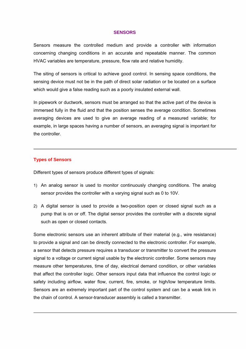
Temperature Sensors
One of the most common properties measured in the HVAC control is temperature. The
principle of measurement involves the thermal expansion of metal or gas, and a calibrated
change in electrical characteristics. Below are common types of temperature sensors:
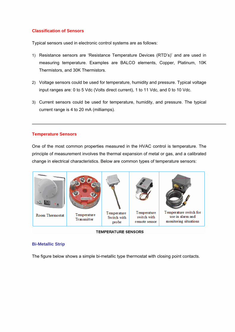
Bi-Metallic Strip
The figure below shows a simple bi-metallic type thermostat with closing point contacts.
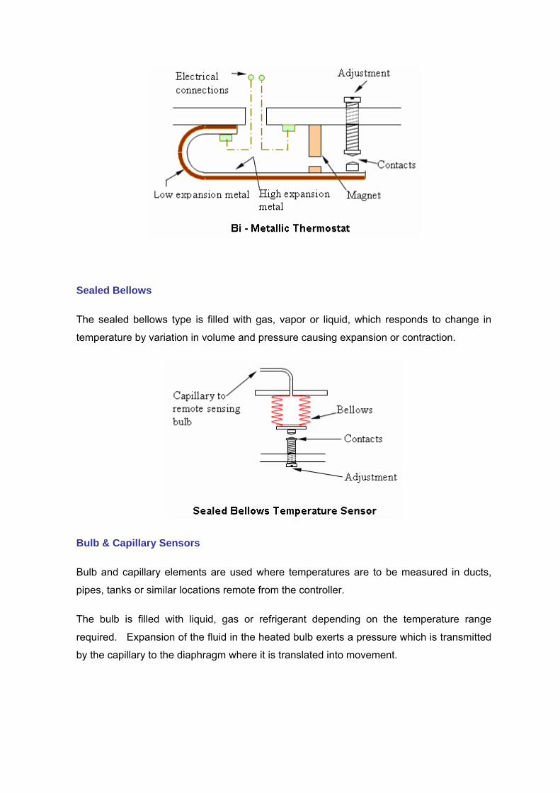
Sealed Bellows
The sealed bellows type is filled with gas, vapor or liquid, which responds to change in
temperature by variation in volume and pressure causing expansion or contraction.
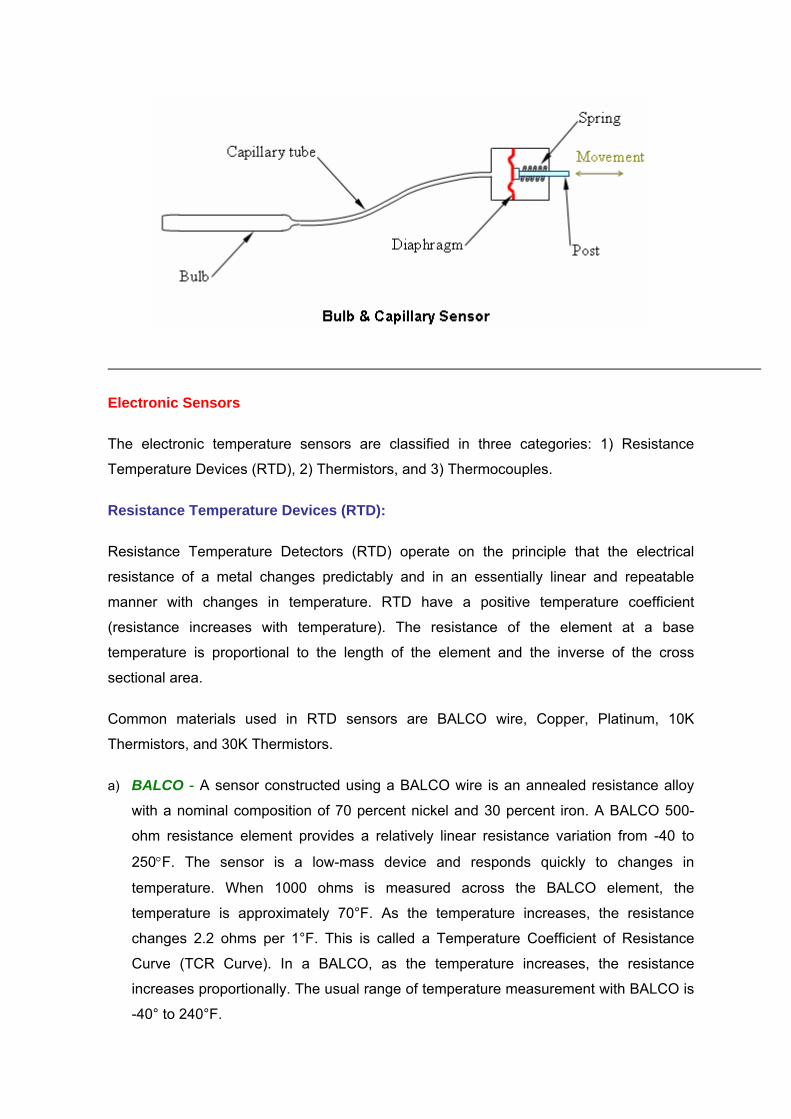
Bulb & Capillary Sensors
Bulb and capillary elements are used where temperatures are to be measured in ducts,
pipes, tanks or similar locations remote from the controller.
The bulb is filled with liquid, gas or refrigerant depending on the temperature range
required. Expansion of the fluid in the heated bulb exerts a pressure which is transmitted
by the capillary to the diaphragm where it is translated into movement.
Electronic Sensors
The electronic temperature sensors are classified in three categories: 1) Resistance
Temperature Devices (RTD), 2) Thermistors, and 3) Thermocouples.
Resistance Temperature Devices (RTD):
Resistance Temperature Detectors (RTD) operate on the principle that the electrical
resistance of a metal changes predictably and in an essentially linear and repeatable
manner with changes in temperature. RTD have a positive temperature coefficient
(resistance increases with temperature). The resistance of the element at a base
temperature is proportional to the length of the element and the inverse of the cross
sectional area.
Common materials used in RTD sensors are BALCO wire, Copper, Platinum, 10K
Thermistors, and 30K Thermistors.
a) BALCO - A sensor constructed using a BALCO wire is an annealed resistance alloy
with a nominal composition of 70 percent nickel and 30 percent iron. A BALCO 500-
ohm resistance element provides a relatively linear resistance variation from -40 to
250°F. The sensor is a low-mass device and responds quickly to changes in
temperature. When 1000 ohms is measured across the BALCO element, the
temperature is approximately 70°F. As the temperature increases, the resistance
changes 2.2 ohms per 1°F. This is called a Temperature Coefficient of Resistance
Curve (TCR Curve). In a BALCO, as the temperature increases, the resistance
increases proportionally. The usual range of temperature measurement with BALCO is
-40° to 240°F.
b) Platinum - RTD sensors using platinum material exhibit linear response and stability
over time. In some applications a short length of wire is used to provide a nominal
resistance of 100 ohms. However, with a low resistance value, element self-heating
and sensor lead wire resistance can effect the temperature indication. With a small
amount of resistance change of the element, additional amplification must be used to
increase the signal level. A platinum film sensor on an insulating base provides high
resistance to the tune of 1000 ohms at 74°F. With this high resistance, the sensor is
relatively immune to self-heating and responds quickly to changes in temperature.
RTD elements of this type are common.
Advantages: Linear resistance with temperature, good stability, wide range of operating
temperature, interchangeable over wide temperature range
Disadvantages: Small resistance change with temperature, responses may be slower,
subject to self heating, three to four wire leads (or transmitter) required for lead resistance
compensation, external circuit power required
Additional facts
1) RTD's are commonly used in sensing air and liquid temperatures in pipes and ducts,
and as room temperature sensors. The resistance of RTD elements varies as a
function of temperature. Some elements exhibit large resistance changes, linear
changes, or both over wide temperature ranges.
2) Varying voltage across the sensor element determines the resistance of the sensor.
The power supplied for this purpose can cause the element to heat slightly and can
create an inaccuracy in the temperature measurement. Reducing supply current or by
using elements with higher nominal resistance can minimize the self-heating effect.
3) Some RTD element resistances are as low as 100 ohms. In these cases, the
resistance of the lead wires connecting the RTD to the controller may add significantly
to the total resistance of the connected RTD, and can create an error in the
measurement of the temperature. For instance, a sensor placed 25 feet from the
controller has a copper control wire of 50 feet (25 x 2). If a control wire has a dc
resistance of 6.39 ohms/ft, the 50 feet of wire will have a total dc resistance of 0.319
ohms. If the sensor is a 100-ohm platinum sensor with a temperature coefficient of
0.69 ohms per degree F, the 50 feet of wire will introduce an error of 0.46 degrees F. If
the sensor is a 3000-ohm platinum sensor with a temperature coefficient of 4.8 ohms
per degree F, the 50 feet of wire will introduce an error of 0.066 degrees F.
Therefore, the lesser is the resistance of a sensor element, the higher will be the
likelihood of an error. Significant errors can be removed by adjusting a calibration
setting on the controller, or, if the controller is designed for it, a third wire can be run to
the sensor and connected to a special compensating circuit designed to remove the
lead length effect on the measurement.
Thermistors
Thermistors are temperature sensitive semiconductors that exhibit a large change in
resistance over a relatively small range of temperatures. There are two main types of
thermistors: positive temperature coefficient (PTC) and negative temperature coefficient
(NTC). NTC thermistors exhibit the characteristic of falling resistance with increasing
temperature. These are most commonly used for temperature measurement.
Unlike RTD's, the temperature-resistance characteristic of a thermistor is non-linear, and
cannot be characterized by a single coefficient. Manufacturers commonly provide
resistance-temperature data in curves, tables or polynomial expressions. Linearizing the
resistance-temperature correlation may be accomplished with analog circuitry, or by the
application of mathematics using digital computation.
Advantages: Large resistance change with temperature, rapid response time, good
stability, high resistance eliminates difficulties caused by lead resistance, low cost and
interchangeable
Disadvantages: Non-linear, limited operating temperature range, may be subjected to
inaccuracy due to overheating, current source required
Thermocouples
Thermocouples have two dissimilar metal wires joined at one end. Temperature
differences at the junction causes a voltage (in the mill volt range) which can be measured
by the input circuits of an electronic controller. The output is a voltage proportional to the
temperature difference between the junction and the free ends. By holding one junction at
a known temperature (reference junction) and measuring the voltage, the temperature at
the sensing junction can be deduced. The voltage generated is directly proportional to the
temperature difference.
At room temperatures for typical HVAC applications, these voltage levels are often too
small to be used, but are more usable at higher temperatures of 200 to 1600°F.
Consequently, thermocouples are most common in high-temperature process applications.
Advantages: Widest operating range, simple, low cost and no external power supply
required.
Disadvantages: Non-linear, low stability relative to other types, reference junction
temperature compensation required
Relative Humidity Sensors
Various sensing methods are used to determine the percentage of relative humidity,
including the measurement of changes of resistance, capacitance, impedance, and
frequency. Fabrics which change dimension with humidity variation, such as hair, nylon or
wood, are still in use as measuring elements but are unreliable. Hygroscopic plastic tape is
now more common. These media may be used to open or close contacts or to operate a
potentiometer. For electronic applications, use is made of a hygroscopic salt such as
lithium chloride, which will provide a change in resistance depending upon the amount of
moisture absorbed. Solid state sensors use polymer film elements to produce variations in
resistance or capacitance.
Resistance Relative Humidity Sensor
A method that uses change in resistance to determine relative humidity works on a layer of
hygroscopic salt, such as lithium chloride deposited between two electrodes. Both
materials absorb and release moisture as a function of the relative humidity, causing a
change in resistance of the sensor. An electronic controller connected to this sensor
detects the changes in resistance which can be used to provide control of relative
humidity.
Capacitance Relative Humidity Sensor
A method that uses changes in capacitance to determine relative humidity measures the
capacitance between two conductive plates separated by a moisture sensitive material
such as polymer plastic. As the material absorbs water, the capacitance between the
plates decreases and the change can be detected by an electronic circuit. To overcome
any hindrance of the material’s ability to absorb and release moisture, the two plates and
their electric lead wires can be on one side of the polymer plastic and a third sheet of
extremely thin conductive material on the other side of the polymer plastic forms the
capacitor. This third plate, too thin for attachment of lead wires, allows moisture to
penetrate and be absorbed by the polymer thus increasing sensitivity and response.
Because of the nature of the measurement, capacitance humidity sensors are combined
with a transmitter to produce a higher-level voltage or current signal. Key considerations in
selection of transmitter sensor combinations include range, temperature limits, end-to-end
accuracy, resolution, long-term stability, and interchangeability.
Capacitance type relative humidity sensor/transmitters are capable of measuring from 0 to
100% relative humidity with application temperatures from -40 to 200 °F. These systems
are manufactured to various tolerances with the most common being accurate to ±1%,
±2%, and ±3%. Capacitance sensors are affected by temperature such that accuracy
decreases as temperature deviates from the calibration temperature. Sensors that are
interchangeable within ±3% without calibration are available. Sensors with long term
stability of <±1% per year are also available.
Temperature Condensation
Both temperature and percent RH affect the output of all absorption based humidity
sensors. Applications calling for either high accuracy or wide temperature operating range
require temperature compensation. The temperature should be made as close as possible
to the RH sensors active area. This is especially true when using RH and temperature to
measure dew-point.
Condensation & Wetting
Condensation occurs whenever the sensor’s surface temperature drops below the dew
point of the surrounding air, even if only momentarily. When operating at levels of 95% RH
and above, small temperature changes can cause condensation.
Under these conditions, where the ambient temperature and the dew-point are very close,
condensation forms quickly but the moisture takes a long time to evaporate. Until the
moisture is gone, the sensor outputs a 100% RH signal.
Quartz Crystal Relative Humidity Sensor
Sensors that use changes in frequency to measure relative humidity can use a quartz
crystal coated with a hygroscopic material such as polymer plastic. When an oscillating
circuit energizes the quartz crystal, it generates a constant frequency. As the polymer
material absorbs moisture and changes the mass of the quartz crystal, the frequency of
oscillation varies and can be measured by an electronic circuit.
Most relative humidity sensors require electronics (referred to as transmitters) at the
sensor to modify and amplify the weak signal. The electronic circuit compensates for the
effects of the temperature as well as amplifies and linearizes the measured level of relative
humidity. The transmitter typically provides a voltage or current output that can be used as
an input to the electronic controller.
When operating in high RH (90% and above), consider these strategies:
1) Maintain good air mixing to minimize local temperature fluctuations.
2) Use a sintered stainless steel filter to protect the sensor from splashing. A hydrophobic
coating can also suppress condensation and wetting in a rapidly saturating/de-
saturating or splash prone environment.
3) Heat the RH sensor above the ambient dew point temperature. (NOTE: Heating the
sensor changes the calibration and makes it sensitive to thermal disturbances such as
airflow.
Pressure Sensors
Diverse electrical principles are applied to pressure measurement. Those commonly used
include capacitance and variable resistance (piezoelectric and strain gage).
Variable Resistance Variable resistance technology includes both strain gage and piezoelectric technologies.
An electronic pressure sensor converts pressure changes into a signal such as voltage,
current, or resistance that can be used by an electronic controller. A method that
measures pressure by detecting changes in resistance uses a small flexible diaphragm
and a strain gage assembly. The strain gage assembly includes very fine (serpentine) wire
or a thin metallic film deposited on a nonconductive base. The strain gage assembly is
stretched or compressed as the diaphragm flexes with pressure variations. The stretching
or compressing of the strain gage changes the length of its fine wire/thin film metal, which
changes the total resistance. The resistance can then be detected and amplified. These
changes in resistance are small. Therefore, an amplifier is provided in the sensor
assembly to amplify and condition the signal so the level sent to the controller is less
susceptible to external noise interference. The sensor thus becomes a transmitter. The
pressure sensing motion may be transmitted directly to an electric or pneumatic control
device. In electronic systems, the diaphragm or the sensing element is connected to a
solid state device which when distorted changes resistivity. This is known as the piezo-
electric effect.
Capacitance
Another pressure sensing method measures capacitance. A fixed plate forms one part of
the capacitor assembly and a flexible plate forms the other part of the capacitor assembly.
As the diaphragm flexes with pressure variations, the flexible plate of the capacitor
assembly moves closer to the fixed plate and changes the capacitance. A variation of
pressure sensor is one that measures differential pressure using dual pressure chambers.
The force from each chamber acts in an opposite direction with respect to the strain gage.
This type of sensor can measure small differential pressure changes even with high static
pressure.
Flow Sensors
Liquid flowrate can be obtained by measuring a velocity of a fluid in a duct or pipe and
multiplying by the known cross sectional area (at the point of measurement) of that duct or
pipe. Common methods used to measure liquid flow include differential pressure
measurement difference across a restriction to flow (orifice plate, flow nozzle, venture),
vortex shedding sensors, positive displacement flow sensors, turbine based flow sensors,
magnetic flow sensors, ultrasonic flow sensors and ‘target’ flow sensors.
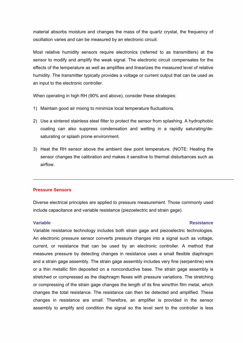
Orifice
A concentric orifice plate is the simplest differential pressure type meter that constrict the
flow of a fluid to produce a differential pressure across the plate. The result is high
pressure upstream and low pressure downstream that is proportional to the square of the
flow velocity. An orifice plate usually produces a greater overall pressure loss than other
flow elements. An advantage of this device is that cost does not increase significantly with
pipe size.
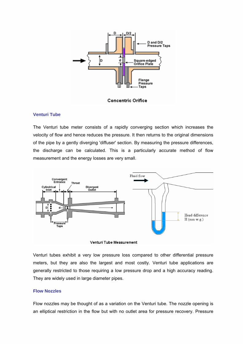
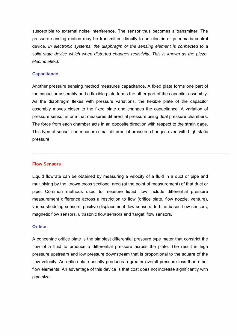
Venturi Tube
The Venturi tube meter consists of a rapidly converging section which increases the
velocity of flow and hence reduces the pressure. It then returns to the original dimensions
of the pipe by a gently diverging 'diffuser' section. By measuring the pressure differences,
the discharge can be calculated. This is a particularly accurate method of flow
measurement and the energy losses are very small.
Venturi tubes exhibit a very low pressure loss compared to other differential pressure
meters, but they are also the largest and most costly. Venturi tube applications are
generally restricted to those requiring a low pressure drop and a high accuracy reading.
They are widely used in large diameter pipes.
Flow Nozzles
Flow nozzles may be thought of as a variation on the Venturi tube. The nozzle opening is
an elliptical restriction in the flow but with no outlet area for pressure recovery. Pressure
taps are located approximately 1/2 pipe diameter downstream and 1 pipe diameter
upstream. The flow nozzle is a high velocity flow meter used where turbulence is high
(Reynolds numbers above 50,000) such as in steam flow at high temperatures. The
pressure drop of a flow nozzle falls between that of the Venturi tube and the orifice plate
(30 to 95 percent).
The turndown (ratio of the full range of the instrument to the minimum measurable flow) of
differential pressure devices is generally limited to 4:1. With the use of a low range
transmitter in addition to a high range transmitter or a high turndown transmitter and
appropriate signal processing, this can sometimes be extended to as great as 16:1 or
more. Permanent pressure loss and associated energy cost are often a major concern in
the selection of orifices, flow nozzles, and venturis. In general, for a given installation, the
permanent pressure loss will be highest with an orifice type device, and lowest with a
Venturi. Benefits of differential pressure instruments are their relatively low cost, simplicity,
and proven performance.
Vortex Shedding Sensors
Vortex shedding flow meters operate on the principle (Von Karman) that when a fluid flows
around an obstruction in the flow stream, vortices are shed from alternating sides of the
obstruction in a repeating and continuous fashion. The frequency at which the shedding
alternates is proportional to the velocity of the flowing fluid. Single sensors are applied to
small ducts, and arrays of vortex shedding sensors are applied to larger ducts, similar to
the other types of airflow measuring instruments. Vortex shedding airflow sensors are
commonly applied to air velocities in the range of 350 to 6000 feet per minute.
Positive Displacement Flow Sensors
Positive displacement meters are used where high accuracy at high turndown is required
and reasonable-to-high permanent pressure loss will not result in excessive energy
consumption. Applications include water metering (such as for potable water service,
cooling tower and boiler make-up) and hydronic system make-up. Positive displacement
meters are also used for fuel metering for both liquid and gaseous fuels. Common types of
positive displacement flow meters include lobed and gear type meters, nutating disk
meters, and oscillating piston type meters. These meters are typically constructed of
metals such as brass, bronze, cast and ductile iron, but may be constructed of engineered
plastic depending on service.
Turbine Based Flow Sensors
Turbine and propeller type meters operate on the principle that fluid flowing through the
turbine or propeller will induce a rotational speed that can be related to the fluid velocity.
Turbine and propeller type flow meters are available in full bore line mounted versions and
insertion types where only a portion of the flow being measured passes over the rotating
element. Full bore turbine and propeller meters generally offer medium to high accuracy
and turndown capability at reasonable permanent pressure loss. Turbine flow meters are
commonly used where good accuracy is required for critical flow control or measurement
for energy computations. Insertion types are used for less critical applications. Insertion
types are often easier to maintain and inspect because they can be removed for inspection
and repair without disturbing the main piping.
Magnetic Flow Sensors
Magnetic flow meters operate based upon Faraday's Law of electromagnetic induction,
which states that a voltage will be induced in a conductor moving through a magnetic field.
Faraday's Law: E= k*B*D*V
The magnitude of the induced voltage E is directly proportional to the velocity of the
conductor V, conductor width D, and the strength of the magnetic field B. The output
voltage E is directly proportional to liquid velocity, resulting in the linear output of a
magnetic flow meter. Magnetic flow meters are used to measure the flow rate of
conducting liquids (including water) where a high quality low maintenance measurement
system is desired. The cost of magnetic flow meters is high relative to many other meter
types.
Ultrasonic Flow Sensors
Ultrasonic flow sensors measure the velocity of sound waves propagating through a fluid
between two points on the length of a pipe. The velocity of the sound wave is dependant
upon the velocity of the fluid such that a sound wave traveling upstream from one point to
the other is slower than the velocity of the same wave in the fluid at rest. The downstream
velocity of the sound wave between the two points is greater than that of the same wave in
a fluid at rest. This is due to the Doppler Effect. The flow of the fluid can be measured as a
function of the difference in time travel between the upstream wave and the downstream
wave.
Ultrasonic flow sensors are non-intrusive and are available at moderate cost. Many
models are designed to clamp on to the existing pipe. Ultrasonic Doppler flow meters have
flow rate accuracies of 1 to 5%.
Air Flow Measurements
Common methods for measuring airflow include hot wire anemometers, differential
pressure measurement systems, and vortex shedding sensors.
Hot Wire Anemometers
Anemometers operate on the principle that the amount of heat removed from a heated
temperature sensor by a flowing fluid can be related to the velocity of that fluid. Most
sensors of this type are constructed with a second unheated temperature sensor to
compensate the instrument for variations in the temperature of the air. Hot wire type
sensors are better at low airflow measurements than differential pressure types, and are
commonly applied to air velocities from 50 to 12,000 feet per minute.
Pitot – Static Tube
The Pitot - static tube can be used to measure total pressure and static pressure through
the ductwork. The diagram below shows a typical Pitot-static tube. The tube facing the air
stream is called the facing tube and measures the total head. The static head is obtained
from the small tapings into the annulus. The head difference, as measured in the
manometer, is therefore the Velocity head.
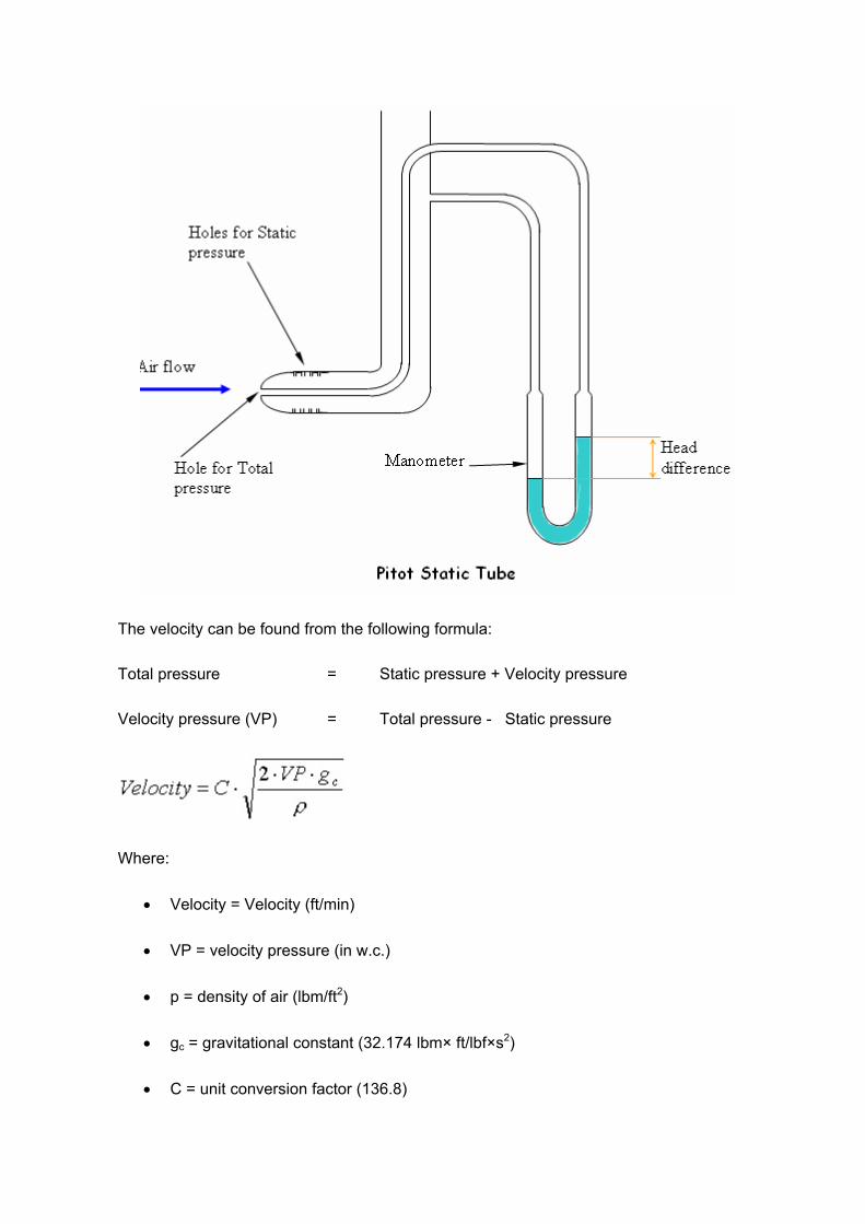
The velocity can be found from the following formula:
Total pressure = Static pressure + Velocity pressure
Velocity pressure (VP) = Total pressure - Static pressure
Where:
• Velocity = Velocity (ft/min)
• VP = velocity pressure (in w.c.)
• p = density of air (lbm/ft2)
• gc = gravitational constant (32.174 lbm× ft/lbf×s2)
• C = unit conversion factor (136.8)
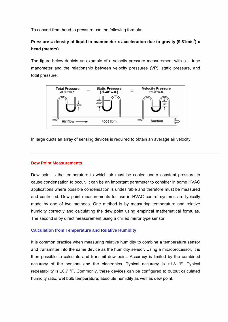
To convert from head to pressure use the following formula:
Pressure = density of liquid in manometer x acceleration due to gravity (9.81m/s2) x head (meters).
The figure below depicts an example of a velocity pressure measurement with a U-tube
manometer and the relationship between velocity pressures (VP), static pressure, and
total pressure.
In large ducts an array of sensing devices is required to obtain an average air velocity.
Dew Point Measurements
Dew point is the temperature to which air must be cooled under constant pressure to
cause condensation to occur. It can be an important parameter to consider in some HVAC
applications where possible condensation is undesirable and therefore must be measured
and controlled. Dew point measurements for use in HVAC control systems are typically
made by one of two methods. One method is by measuring temperature and relative
humidity correctly and calculating the dew point using empirical mathematical formulas.
The second is by direct measurement using a chilled mirror type sensor.
Calculation from Temperature and Relative Humidity
It is common practice when measuring relative humidity to combine a temperature sensor
and transmitter into the same device as the humidity sensor. Using a microprocessor, it is
then possible to calculate and transmit dew point. Accuracy is limited by the combined
accuracy of the sensors and the electronics. Typical accuracy is ±1.8 °F. Typical
repeatability is ±0.7 °F. Commonly, these devices can be configured to output calculated
humidity ratio, wet bulb temperature, absolute humidity as well as dew point.
Chilled Mirror Hygrometers
Modern chilled mirror hygrometers use a thermoelectric heat pump (also called a Peltier
device) to move heat away from a mirror. A light beam from an LED is directed to the
mirror and back to a photocell. When condensation (above 0 °C) or frost (below 0 °C)
forms on the mirror’s surface, the light reaching the mirror is scattered and the intensity
detected by the photocell is reduced. The mirror is maintained at the dew point
temperature by controlling the output of the thermoelectric heat pump. A high accuracy
platinum resistance thermometer (RTD) senses the temperature of the mirror’s surface
and therefore reports the dew point temperature. Chilled mirror hygrometers require a
vacuum pump to draw the sample through the sensor, and additional filtration elements in
dirty environments. Chilled mirror hygrometers are available for sensing dew/frost point
temperatures from -100 to 185 °F. Accuracy of better than ± 0.5 °F is available.
Liquid Level Measurements
Liquid level measurements are typically used to monitor and control levels in thermal
storage tanks, cooling tower sumps, water system tanks, pressurized tanks, etc. Common
technologies applicable to HVAC system requirements are based on hydrostatic pressure,
ultrasonic, capacitance and magnetostrictive-based measurement systems.
Hydrostatic Level measurement by hydrostatic pressure is based on the principle that the hydrostatic
pressure difference between the top and bottom of a column of liquid is related to the
density of the liquid and the height of the column. For open tanks and sumps, it is only
necessary to measure the gauge pressure at the lowest monitored level. For pressurized
tanks it is necessary to take the reference pressure above the highest monitored liquid
level. Pressure transmitters that are configured for level monitoring applications are
available. Pressure instruments may also be remotely located; however, this makes it
necessary to field calibrate the transmitter to compensate for the elevation difference
between the sensor and the level being measured.
Bubbler type hydrostatic level instruments have been developed for use with atmospheric
pressure underground tanks, sewage sumps and tanks, and other applications that cannot
have a transmitter mounted below the level being sensed or are prone to plugging.
Bubbler systems bleed a small amount of compressed air (or other gas) through a tube
that is immersed in the liquid, with an outlet at or below the lowest monitored liquid level.
The flow rate of the air is regulated so that the pressure loss of the air in the tube is
negligible and the resulting pressure at any point in the tube is approximately equal to the
hydrostatic head of the liquid in the tank. The accuracy of hydrostatic level instruments is
related to the accuracy of the pressure sensor used.
Ultrasonic
Ultrasonic level sensors emit sound waves and operate on the principle that liquid
surfaces reflect the sound waves back to the source and that the transit time is
proportional to the distance between the liquid surface and the transmitter. One advantage
of the ultrasonic technology is that it is non-contact and does not require immersion of any
element into the sensed liquid. Sensors that can detect levels up to 200 feet from the
sensor are available. Accuracy from 1% to 0.25% of distance and resolution of 1/8" is
commonly available.
Capacitance
Capacitance level transmitters operate on the principle that a capacitive circuit can be
formed between a probe and a vessel wall. The capacitance of the circuit will change with
a change in fluid level because all common liquids have a dielectric constant higher than
that of air. This change is then related proportionally to an analog signal.
CONTROLLERS
The controller receives signals from the sensor, compares inputs with a set of instructions
(such as setpoint, throttling range), applies control logic and then produces an output
signal. The output signal may be transmitted either to the controlled device or to other
logical control functions. The type of signals from the controllers can be electric, electronic,
pneumatic or digital. The electronic signals could either be voltage or current outputs.
Voltage outputs may be 0 to 10 Vdc, 2 to 15 Vdc, or other ranges depending on the
controller. Voltage outputs have the disadvantage, when compared to current signals, that
voltage signals are more susceptible to distortion over long wire distances. Current outputs
modulate from 4 to 20 mA. They have the advantage of producing little signal distortion
over long wire distances.
Controller Action
All controllers, from pneumatic to electronic, have an action. They are either ‘Direct Acting’
or ‘Reverse Acting’.
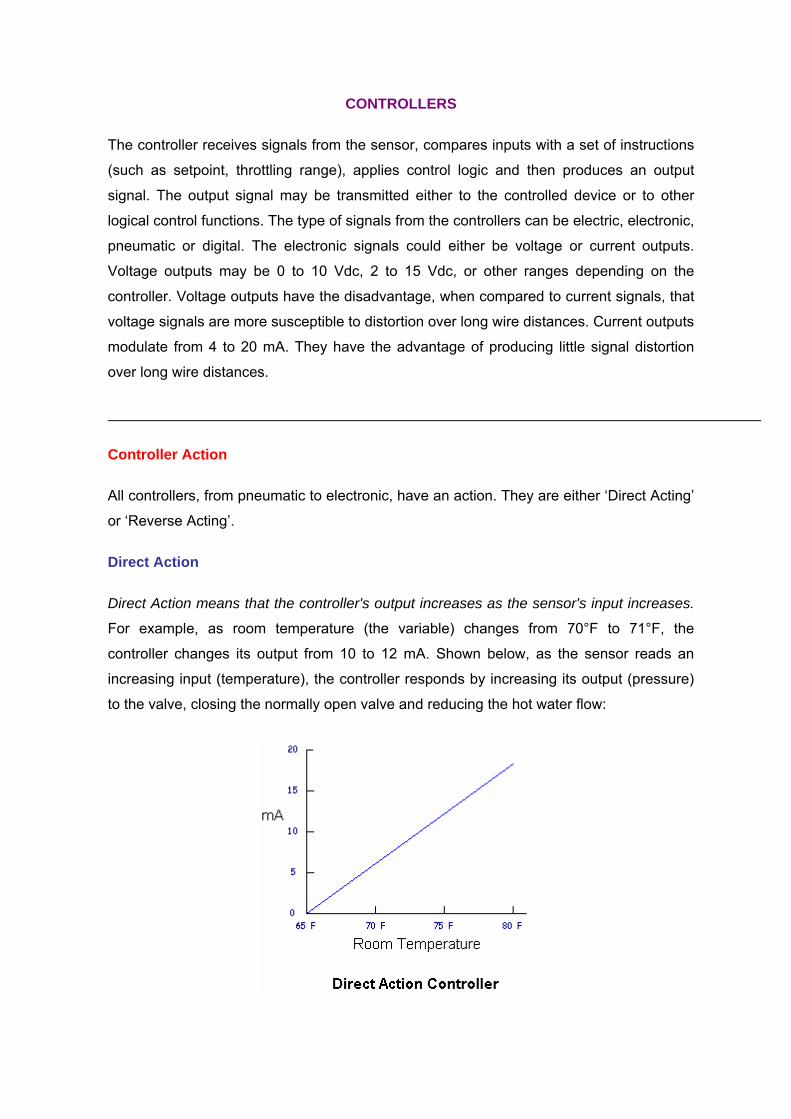
Direct Action
Direct Action means that the controller's output increases as the sensor's input increases.
For example, as room temperature (the variable) changes from 70°F to 71°F, the
controller changes its output from 10 to 12 mA. Shown below, as the sensor reads an
increasing input (temperature), the controller responds by increasing its output (pressure)
to the valve, closing the normally open valve and reducing the hot water flow:
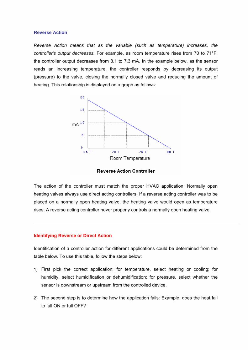
Reverse Action
Reverse Action means that as the variable (such as temperature) increases, the
controller's output decreases. For example, as room temperature rises from 70 to 71°F,
the controller output decreases from 8.1 to 7.3 mA. In the example below, as the sensor
reads an increasing temperature, the controller responds by decreasing its output
(pressure) to the valve, closing the normally closed valve and reducing the amount of
heating. This relationship is displayed on a graph as follows:
The action of the controller must match the proper HVAC application. Normally open
heating valves always use direct acting controllers. If a reverse acting controller was to be
placed on a normally open heating valve, the heating valve would open as temperature
rises. A reverse acting controller never properly controls a normally open heating valve.
Identifying Reverse or Direct Action
Identification of a controller action for different applications could be determined from the
table below. To use this table, follow the steps below:
1) First pick the correct application: for temperature, select heating or cooling; for
humidity, select humidification or dehumidification; for pressure, select whether the
sensor is downstream or upstream from the controlled device.
2) The second step is to determine how the application fails: Example, does the heat fail
to full ON or full OFF?
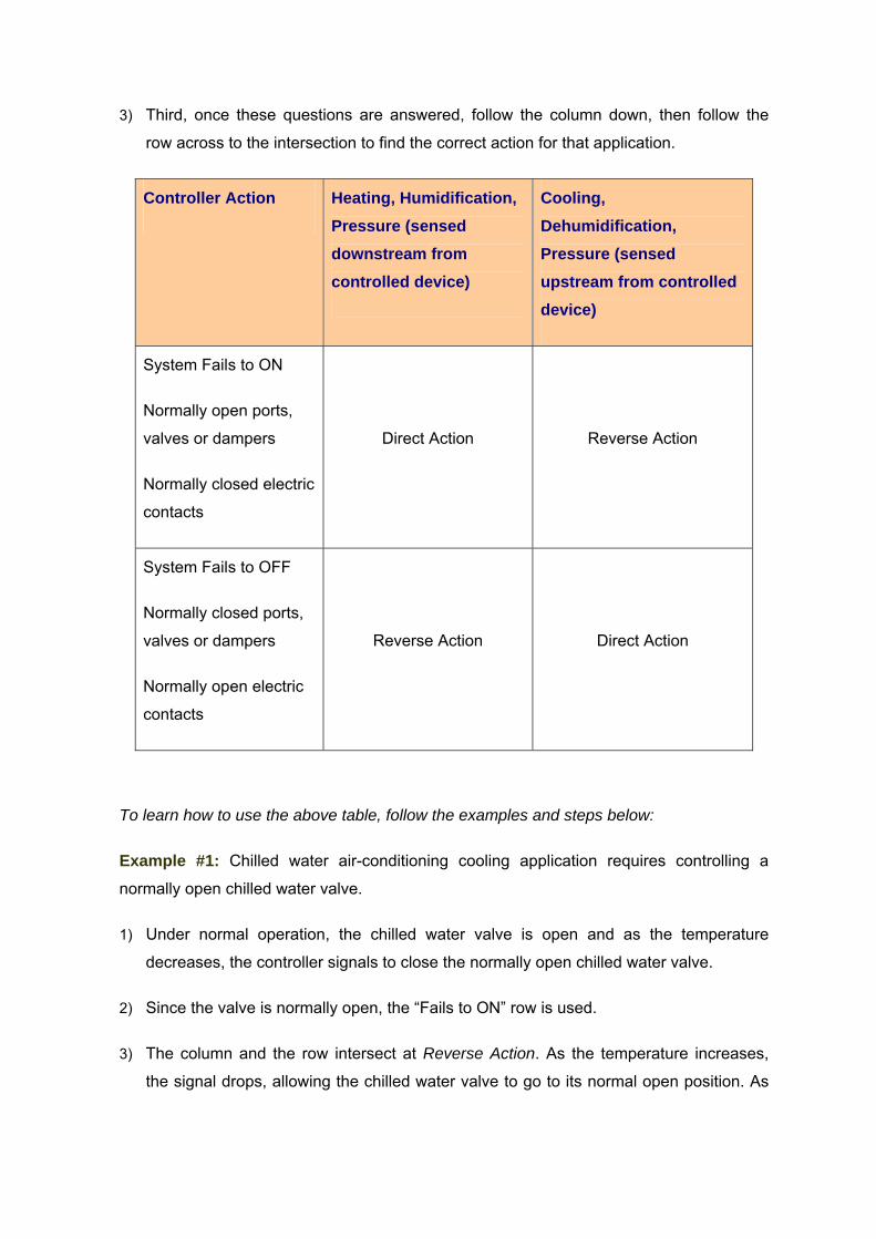
3) Third, once these questions are answered, follow the column down, then follow the
row across to the intersection to find the correct action for that application.
Controller Action Heating, Humidification, Pressure (sensed downstream from controlled device)
Cooling, Dehumidification, Pressure (sensed upstream from controlled device)
System Fails to ON
Normally open ports,
valves or dampers
Normally closed electric
contacts
Direct Action Reverse Action
System Fails to OFF
Normally closed ports,
valves or dampers
Normally open electric
contacts
Reverse Action Direct Action
To learn how to use the above table, follow the examples and steps below:
Example #1: Chilled water air-conditioning cooling application requires controlling a
normally open chilled water valve.
1) Under normal operation, the chilled water valve is open and as the temperature
decreases, the controller signals to close the normally open chilled water valve.
2) Since the valve is normally open, the “Fails to ON” row is used.
3) The column and the row intersect at Reverse Action. As the temperature increases,
the signal drops, allowing the chilled water valve to go to its normal open position. As
the temperature decreases, the signal increases, closing the normally open chilled
water valve.
Example # 2: A return air humidity sensor modulates a normally closed chilled water valve
for dehumidification. What action is needed for the controller?
Direct Action
Example #3: A static pressure sensor (located on the discharge side) modulates the
normally closed inlet vane dampers to maintain 2.0" w.c. (500 Pa). What action is needed
for the controller?
Reverse Action
Example #4: A room sensor cycles DX cooling to maintain a room temperature at 75°F.
The DX Cooling has normally open electrical contacts. What action is needed for the
controller?
Direct Action
Example #5: The mixed air sensor (located on the discharge side) modulates the normally
closed outside air dampers and the normally open return air dampers to maintain a
temperature of 55°F. What action is needed for the controller?
Direct Action
CONTROLLER TYPES
Temperature Controllers
A temperature controller, as the name implies, is an instrument used to control
temperature. The temperature controller takes the input from a temperature sensor and
provides an output that is connected to a control element such as a heater or fan.
Temperature controllers typically require a specific type or category of input sensors.
Some have input circuits to accept RTD sensors such as BALCO or platinum elements,
while others contain input circuits for thermistor sensors. These controllers have setpoint
and throttling range scales labeled in degrees F or C.
Relative Humidity Controllers
The input circuits for relative humidity controllers typically receive the sensed relative
humidity signal already converted to a 0 to 10V dc voltage or 4-to 20 mA current signals.
Setpoint and scales for these controllers are in percent relative humidity.
Enthalpy Controllers
Enthalpy controllers are specialized devices that use specific sensors for inputs. In some
cases, the sensor may combine temperature and humidity measurements and convert
them to a single voltage to represent enthalpy of the sensed air. In other cases, individual
dry bulb temperature sensors and separate wet bulb or relative humidity sensors provide
inputs and the controller calculates enthalpy. In typical applications, the enthalpy controller
provides an output signal based on a comparison of two enthalpy measurements (indoor
and outdoor) rather than on the actual enthalpy value. In other cases, the return air
enthalpy is assumed constant so that only outdoor air enthalpy is measured. It is
compared against the assumed nominal return air value.
Universal Controllers
The input circuits of a universal controller can accept one or more of the standard
transmitter/transducer signals. The most common input ranges are 0 to 10V dc and 4 to 20
mA. Other input variations in this category include a 2 to 10V dc and a 0 to 20 mA signal.
Because these inputs can represent a variety of sensed variables such as a current of 0 to
15 amperes or pressure of 0 to 3000 psi, the settings and scales are often expressed in
percent of full scale only.
RESET
The “reset” in HVAC applications is the automatic resetting of a setpoint based on a
secondary signal. Reset of a setpoint is used for comfort reasons, for better control, or to
save energy. A common example of reset is called hot water reset. Hot water reset
automatically decreases the hot water temperature setpoint as the outside air temperature
rises. If the outside air temperature is 0°F, the building requires 180°F water, and if the
outside air temperature is 70°F, the building requires 90°F water. As the outside
temperature increases, the hot water setpoint drops.
In every reset application there are at least two sensors: primary and secondary sensors.
In the example above, the two sensors are outside air temperature (OA Temp) and hot
water supply temperature (HWS). To determine which of the two is the primary sensor,
one needs to determine what are the controls trying to control?"
In the example above, the hot water temperature is being controlled; therefore the hot
water sensor is the primary sensor. The outside air temperature sensor is the secondary
sensor. The function of the secondary sensor is to reset or automatically change the
setpoint of the controller. Each reset application uses a reset schedule. This schedule is
determined by the mechanical engineer or the application engineer.
Just as the term controller action is defined as reverse and direct, the term reset is also
defined as reverse and direct. The hot water reset example is a reverse reset. Reverse
reset is the most common.
Reverse Reset
Reverse reset means that as the signal from the secondary sensor drops, the setpoint of
the controller increases. In the example above, as the outside air temperature drops, the
hot water setpoint rises.
Direct Reset
With direct reset, as the signal for the secondary input increases, the setpoint increases.
Direct reset is less common than reverse reset. An example of direct reset is an
application called “summer compensation”, shown below.
When cooling (air conditioning) was first introduced, shopping malls advertised their stores
as being a comfortable 72°F year round. This was fine until the summer became very hot.
People who were outside in 100°F weather, dressed for hot weather, would walk into a
shopping mall and feel cold. Some people did not stay long in the stores because it felt too
cool. Summer compensation is used to counteract this problem. Summer compensation
raises the zone setpoint as the outside air temperature increases. The secondary signal
and the setpoint go in the same direction. A typical reset schedule for this application may
look like the following:
Summer Compensation Reset Schedule
OA Temp Zone Setpoint
72°F 72°F
105°F 78°F
This application is used in any building where a large number of people are entering and
leaving all day, such as a shopping mall or bank. If this application is used, it may be
important to ensure that the air is dehumidified for proper comfort.
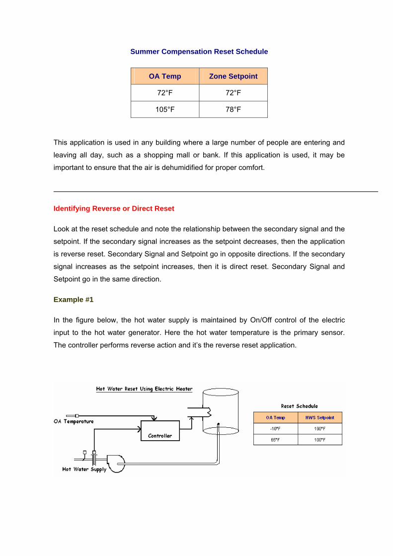
Identifying Reverse or Direct Reset
Look at the reset schedule and note the relationship between the secondary signal and the
setpoint. If the secondary signal increases as the setpoint decreases, then the application
is reverse reset. Secondary Signal and Setpoint go in opposite directions. If the secondary
signal increases as the setpoint increases, then it is direct reset. Secondary Signal and
Setpoint go in the same direction.
Example #1
In the figure below, the hot water supply is maintained by On/Off control of the electric
input to the hot water generator. Here the hot water temperature is the primary sensor.
The controller performs reverse action and it’s the reverse reset application.
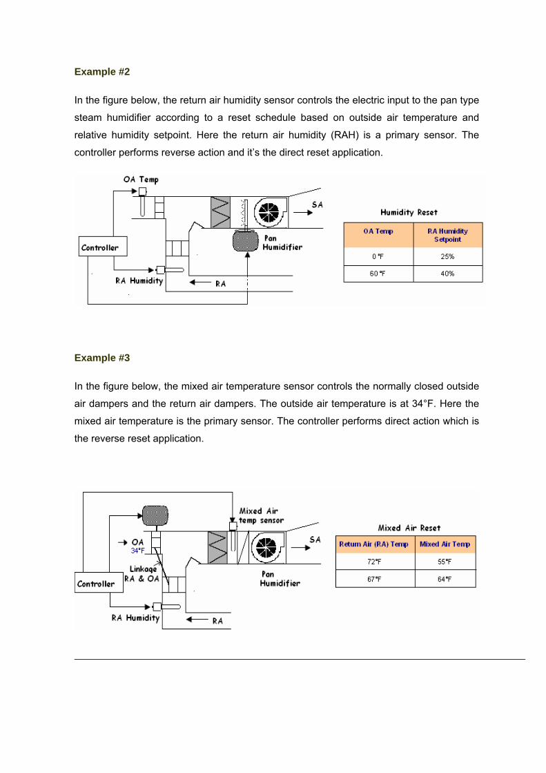
Example #2
In the figure below, the return air humidity sensor controls the electric input to the pan type
steam humidifier according to a reset schedule based on outside air temperature and
relative humidity setpoint. Here the return air humidity (RAH) is a primary sensor. The
controller performs reverse action and it’s the direct reset application.
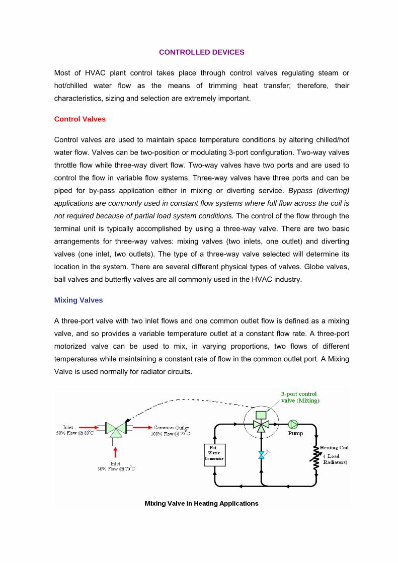
Example #3
In the figure below, the mixed air temperature sensor controls the normally closed outside
air dampers and the return air dampers. The outside air temperature is at 34°F. Here the
mixed air temperature is the primary sensor. The controller performs direct action which is
the reverse reset application.
CONTROLLED DEVICES
Most of HVAC plant control takes place through control valves regulating steam or
hot/chilled water flow as the means of trimming heat transfer; therefore, their
characteristics, sizing and selection are extremely important.
Control Valves
Control valves are used to maintain space temperature conditions by altering chilled/hot
water flow. Valves can be two-position or modulating 3-port configuration. Two-way valves
throttle flow while three-way divert flow. Two-way valves have two ports and are used to
control the flow in variable flow systems. Three-way valves have three ports and can be
piped for by-pass application either in mixing or diverting service. Bypass (diverting)
applications are commonly used in constant flow systems where full flow across the coil is
not required because of partial load system conditions. The control of the flow through the
terminal unit is typically accomplished by using a three-way valve. There are two basic
arrangements for three-way valves: mixing valves (two inlets, one outlet) and diverting
valves (one inlet, two outlets). The type of a three-way valve selected will determine its
location in the system. There are several different physical types of valves. Globe valves,
ball valves and butterfly valves are all commonly used in the HVAC industry.
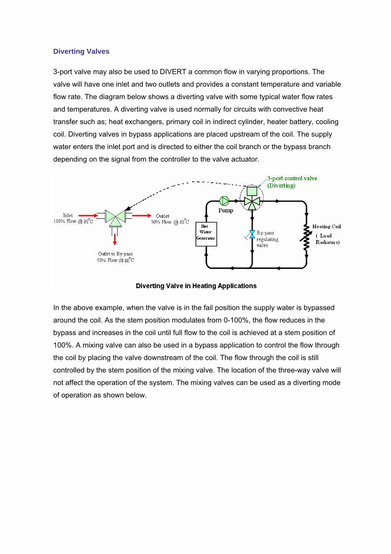
Mixing Valves
A three-port valve with two inlet flows and one common outlet flow is defined as a mixing
valve, and so provides a variable temperature outlet at a constant flow rate. A three-port
motorized valve can be used to mix, in varying proportions, two flows of different
temperatures while maintaining a constant rate of flow in the common outlet port. A Mixing
Valve is used normally for radiator circuits.
Diverting Valves
3-port valve may also be used to DIVERT a common flow in varying proportions. The
valve will have one inlet and two outlets and provides a constant temperature and variable
flow rate. The diagram below shows a diverting valve with some typical water flow rates
and temperatures. A diverting valve is used normally for circuits with convective heat
transfer such as; heat exchangers, primary coil in indirect cylinder, heater battery, cooling
coil. Diverting valves in bypass applications are placed upstream of the coil. The supply
water enters the inlet port and is directed to either the coil branch or the bypass branch
depending on the signal from the controller to the valve actuator.
In the above example, when the valve is in the fail position the supply water is bypassed
around the coil. As the stem position modulates from 0-100%, the flow reduces in the
bypass and increases in the coil until full flow to the coil is achieved at a stem position of
100%. A mixing valve can also be used in a bypass application to control the flow through
the coil by placing the valve downstream of the coil. The flow through the coil is still
controlled by the stem position of the mixing valve. The location of the three-way valve will
not affect the operation of the system. The mixing valves can be used as a diverting mode
of operation as shown below.
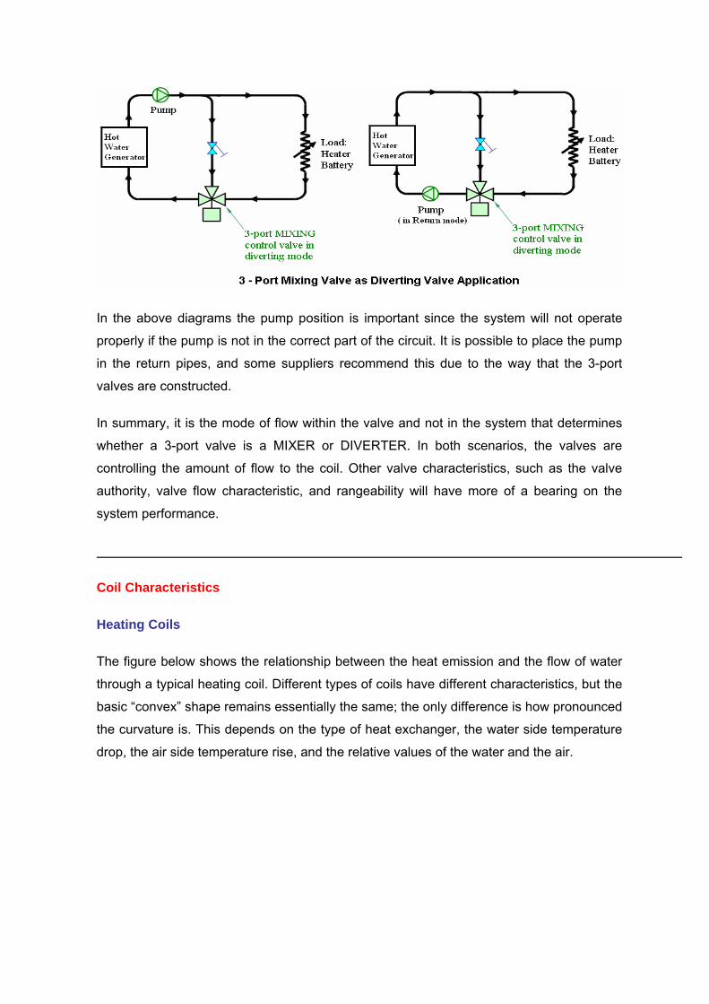
In the above diagrams the pump position is important since the system will not operate
properly if the pump is not in the correct part of the circuit. It is possible to place the pump
in the return pipes, and some suppliers recommend this due to the way that the 3-port
valves are constructed.
In summary, it is the mode of flow within the valve and not in the system that determines
whether a 3-port valve is a MIXER or DIVERTER. In both scenarios, the valves are
controlling the amount of flow to the coil. Other valve characteristics, such as the valve
authority, valve flow characteristic, and rangeability will have more of a bearing on the
system performance.
Coil Characteristics
Heating Coils
The figure below shows the relationship between the heat emission and the flow of water
through a typical heating coil. Different types of coils have different characteristics, but the
basic “convex” shape remains essentially the same; the only difference is how pronounced
the curvature is. This depends on the type of heat exchanger, the water side temperature
drop, the air side temperature rise, and the relative values of the water and the air.
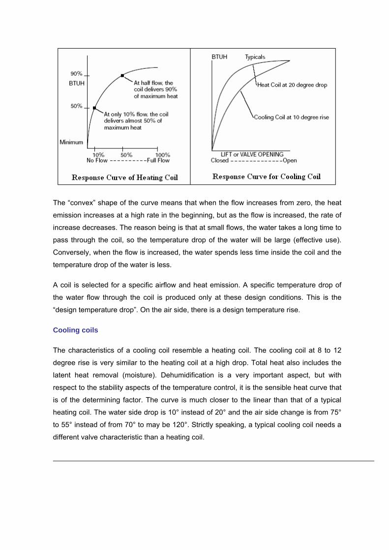
The “convex” shape of the curve means that when the flow increases from zero, the heat
emission increases at a high rate in the beginning, but as the flow is increased, the rate of
increase decreases. The reason being is that at small flows, the water takes a long time to
pass through the coil, so the temperature drop of the water will be large (effective use).
Conversely, when the flow is increased, the water spends less time inside the coil and the
temperature drop of the water is less.
A coil is selected for a specific airflow and heat emission. A specific temperature drop of
the water flow through the coil is produced only at these design conditions. This is the
“design temperature drop”. On the air side, there is a design temperature rise.
Cooling coils
The characteristics of a cooling coil resemble a heating coil. The cooling coil at 8 to 12
degree rise is very similar to the heating coil at a high drop. Total heat also includes the
latent heat removal (moisture). Dehumidification is a very important aspect, but with
respect to the stability aspects of the temperature control, it is the sensible heat curve that
is of the determining factor. The curve is much closer to the linear than that of a typical
heating coil. The water side drop is 10° instead of 20° and the air side change is from 75°
to 55° instead of from 70° to may be 120°. Strictly speaking, a typical cooling coil needs a
different valve characteristic than a heating coil.
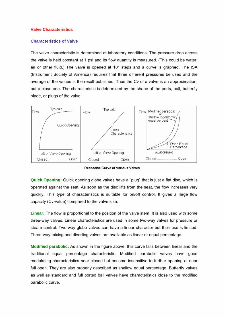
Valve Characteristics
Characteristics of Valve
The valve characteristic is determined at laboratory conditions. The pressure drop across
the valve is held constant at 1 psi and its flow quantity is measured. (This could be water,
air or other fluid.) The valve is opened at 10° steps and a curve is graphed. The ISA
(Instrument Society of America) requires that three different pressures be used and the
average of the values is the result published. Thus the Cv of a valve is an approximation,
but a close one. The characteristic is determined by the shape of the ports, ball, butterfly
blade, or plugs of the valve.
Quick Opening: Quick opening globe valves have a “plug” that is just a flat disc, which is
operated against the seat. As soon as the disc lifts from the seat, the flow increases very
quickly. This type of characteristics is suitable for on/off control. It gives a large flow
capacity (Cv-value) compared to the valve size.
Linear: The flow is proportional to the position of the valve stem. It is also used with some
three-way valves. Linear characteristics are used in some two-way valves for pressure or
steam control. Two-way globe valves can have a linear character but their use is limited.
Three-way mixing and diverting valves are available as linear or equal percentage.
Modified parabolic: As shown in the figure above, this curve falls between linear and the
traditional equal percentage characteristic. Modified parabolic valves have good
modulating characteristics near closed but become insensitive to further opening at near
full open. They are also properly described as shallow equal percentage. Butterfly valves
as well as standard and full ported ball valves have characteristics close to the modified
parabolic curve.
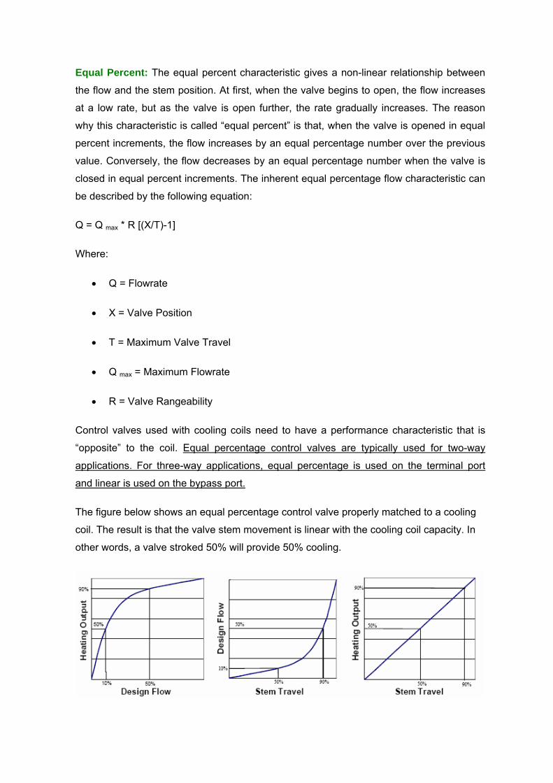
Equal Percent: The equal percent characteristic gives a non-linear relationship between
the flow and the stem position. At first, when the valve begins to open, the flow increases
at a low rate, but as the valve is open further, the rate gradually increases. The reason
why this characteristic is called “equal percent” is that, when the valve is opened in equal
percent increments, the flow increases by an equal percentage number over the previous
value. Conversely, the flow decreases by an equal percentage number when the valve is
closed in equal percent increments. The inherent equal percentage flow characteristic can
be described by the following equation:
Q = Q max * R [(X/T)-1]
Where:
• Q = Flowrate
• X = Valve Position
• T = Maximum Valve Travel
• Q max = Maximum Flowrate
• R = Valve Rangeability
Control valves used with cooling coils need to have a performance characteristic that is
“opposite” to the coil. Equal percentage control valves are typically used for two-way
applications. For three-way applications, equal percentage is used on the terminal port
and linear is used on the bypass port.
The figure below shows an equal percentage control valve properly matched to a cooling
coil. The result is that the valve stem movement is linear with the cooling coil capacity. In
other words, a valve stroked 50% will provide 50% cooling.
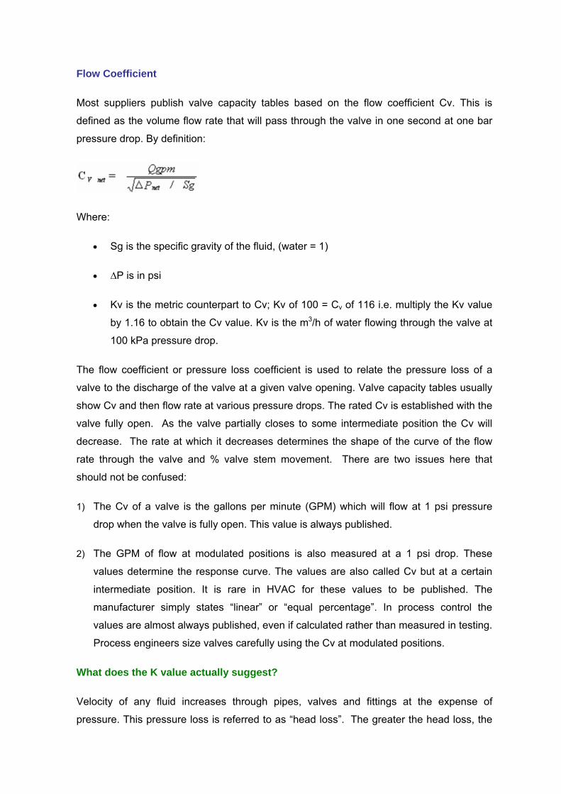
Flow Coefficient
Most suppliers publish valve capacity tables based on the flow coefficient Cv. This is
defined as the volume flow rate that will pass through the valve in one second at one bar
pressure drop. By definition:
Where:
• Sg is the specific gravity of the fluid, (water = 1)
• ∆P is in psi
• Kv is the metric counterpart to Cv; Kv of 100 = Cv of 116 i.e. multiply the Kv value
by 1.16 to obtain the Cv value. Kv is the m3/h of water flowing through the valve at
100 kPa pressure drop.
The flow coefficient or pressure loss coefficient is used to relate the pressure loss of a
valve to the discharge of the valve at a given valve opening. Valve capacity tables usually
show Cv and then flow rate at various pressure drops. The rated Cv is established with the
valve fully open. As the valve partially closes to some intermediate position the Cv will
decrease. The rate at which it decreases determines the shape of the curve of the flow
rate through the valve and % valve stem movement. There are two issues here that
should not be confused:
1) The Cv of a valve is the gallons per minute (GPM) which will flow at 1 psi pressure
drop when the valve is fully open. This value is always published.
2) The GPM of flow at modulated positions is also measured at a 1 psi drop. These
values determine the response curve. The values are also called Cv but at a certain
intermediate position. It is rare in HVAC for these values to be published. The
manufacturer simply states “linear” or “equal percentage”. In process control the
values are almost always published, even if calculated rather than measured in testing.
Process engineers size valves carefully using the Cv at modulated positions.
What does the K value actually suggest?
Velocity of any fluid increases through pipes, valves and fittings at the expense of
pressure. This pressure loss is referred to as “head loss”. The greater the head loss, the
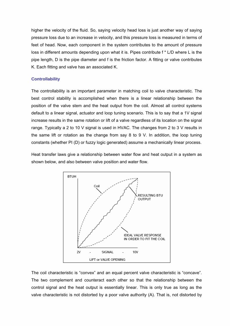
higher the velocity of the fluid. So, saying velocity head loss is just another way of saying
pressure loss due to an increase in velocity, and this pressure loss is measured in terms of
feet of head. Now, each component in the system contributes to the amount of pressure
loss in different amounts depending upon what it is. Pipes contribute f * L/D where L is the
pipe length, D is the pipe diameter and f is the friction factor. A fitting or valve contributes
K. Each fitting and valve has an associated K.
Controllability
The controllability is an important parameter in matching coil to valve characteristic. The
best control stability is accomplished when there is a linear relationship between the
position of the valve stem and the heat output from the coil. Almost all control systems
default to a linear signal, actuator and loop tuning scenario. This is to say that a 1V signal
increase results in the same rotation or lift of a valve regardless of its location on the signal
range. Typically a 2 to 10 V signal is used in HVAC. The changes from 2 to 3 V results in
the same lift or rotation as the change from say 8 to 9 V. In addition, the loop tuning
constants (whether PI (D) or fuzzy logic generated) assume a mechanically linear process.
Heat transfer laws give a relationship between water flow and heat output in a system as
shown below, and also between valve position and water flow.
The coil characteristic is “convex” and an equal percent valve characteristic is “concave”.
The two complement and counteract each other so that the relationship between the
control signal and the heat output is essentially linear. This is only true as long as the
valve characteristic is not distorted by a poor valve authority (A). That is, not distorted by
too low an authority. It is obvious that in order to get a stable control, a high valve authority
is desirable.
Resolution & Let-By
Resolution is the number of positions an actuator will assume when the control signal is
slowly changed form 0 to 100%. (You could also call it “positioning accuracy”). In
installations where it is difficult to get a valve to seat properly there will be a percentage of
let-by. A 2% let-by is normal for a double seat valve but some valves have a let-by of only
0.2%, if a reasonably tight shut-off is possible on a metal to metal seat. A soft seat may be
made from neoprene rubber to give an absolute tight shut-off where necessary.
Rangeability Factor
This describes the ability of a valve to stay on its theoretical characteristic at the bottom
end near the closed position. This is the minimum value that should be considered if good
control on light load is to be achieved. The ratio between the full flow and the minimum
controllable flow is the rangeability factor.
The rangeability factor is measured under laboratory conditions with a constant differential
pressure applied across the valve. Rangeability is a characteristic of the valve itself and it
depends on its design and tolerances.
Turndown Ratio
This is the ratio between the maximum normal flow and the minimum controllable flow. It is
substantially less than the range ability if the valve is oversized, either by error or
deliberately to allow for an occasional peak load.
The higher the turndown ratio is, the better the controllability will be. The turndown ratio
relates to installed valves only and is always smaller than the rangeability factor. The
actuator affects turndown. An actuator with a high accuracy has a 200:1 possible
rangeability (8V span / .04V response).
Example
In a laboratory, a constant differential pressure of 10 PSI is applied across the valve. The
maximum flow is 100 GPM and the minimum controllable flow is 2 GPM. Thus, the
rangeability factor is RF = 100/2 = 50:1.
Valve Authority
As a control valve closes, the pressure drop across the valve increases so that when the
valve is completely closed, the differential pressure drop across the valve matches the
pressure drop from the supply to the return line. This pressure drop is known as ∆P-max.
When the valve is completely open, the pressure drop across the valve is at its lowest
point and is referred to ∆P-min.
The ratio (N) = ∆P min ÷ ∆P max which is the valve authority.
The increase in pressure drop across the valve as it closes is important to note. Valves are
rated based on a constant pressure drop. As the pressure drop shifts, the performance of
the valve changes. The method to minimize the change in valve performance is to
maintain the Valve Authority (N) above 0.5.
Example
Consider a control valve with a Cv = 25 serving a coil that has a design flow of 50 GPM.
The pressure differential from the supply to the return line is 16 PSI.
As the valve closes, the system pressure shifts to the valve until the entire pressure drop
(16 PSI) is across the valve. If the valve was fully opened and there was 16 PSI across the
valve, the flow rate would increase to:
Q = Cv * (∆P) ½ = 25 * (16) ½ = 100 GPM
This does not actually happen; however, since the pressure drops through the coil,
balancing valve, etc., it increases and limits the flow to 50 GPM.
∆P-min = (Q) ²/ (Cv) ² = (50)²/ (25)² = 4 PSI
In this case, the valve authority (N) is 4 PSI/16 PSI = 0.25. This will not provide a linear
relationship between valve position and coil output. This can lead to poor coil performance
and low delta T syndrome. The solution is to try and keep the valve authority above 0.5. In
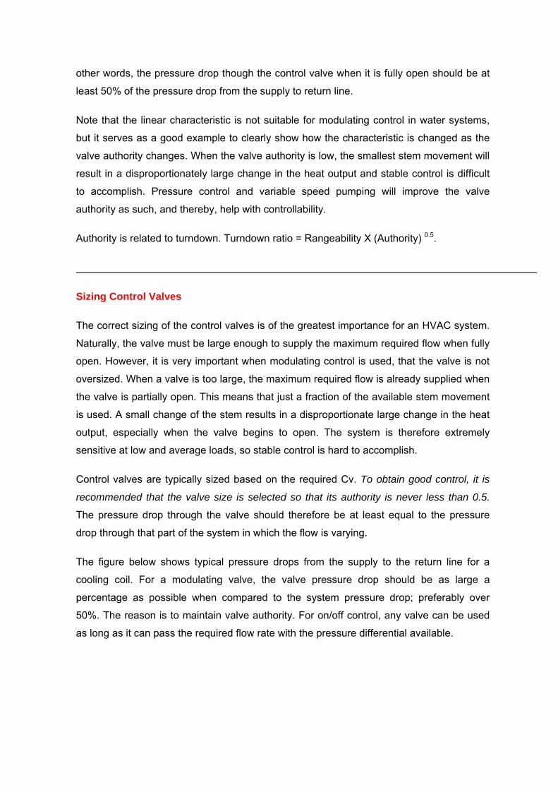
other words, the pressure drop though the control valve when it is fully open should be at
least 50% of the pressure drop from the supply to return line.
Note that the linear characteristic is not suitable for modulating control in water systems,
but it serves as a good example to clearly show how the characteristic is changed as the
valve authority changes. When the valve authority is low, the smallest stem movement will
result in a disproportionately large change in the heat output and stable control is difficult
to accomplish. Pressure control and variable speed pumping will improve the valve
authority as such, and thereby, help with controllability.
Authority is related to turndown. Turndown ratio = Rangeability X (Authority) 0.5.
Sizing Control Valves
The correct sizing of the control valves is of the greatest importance for an HVAC system.
Naturally, the valve must be large enough to supply the maximum required flow when fully
open. However, it is very important when modulating control is used, that the valve is not
oversized. When a valve is too large, the maximum required flow is already supplied when
the valve is partially open. This means that just a fraction of the available stem movement
is used. A small change of the stem results in a disproportionate large change in the heat
output, especially when the valve begins to open. The system is therefore extremely
sensitive at low and average loads, so stable control is hard to accomplish.
Control valves are typically sized based on the required Cv. To obtain good control, it is
recommended that the valve size is selected so that its authority is never less than 0.5.
The pressure drop through the valve should therefore be at least equal to the pressure
drop through that part of the system in which the flow is varying.
The figure below shows typical pressure drops from the supply to the return line for a
cooling coil. For a modulating valve, the valve pressure drop should be as large a
percentage as possible when compared to the system pressure drop; preferably over
50%. The reason is to maintain valve authority. For on/off control, any valve can be used
as long as it can pass the required flow rate with the pressure differential available.
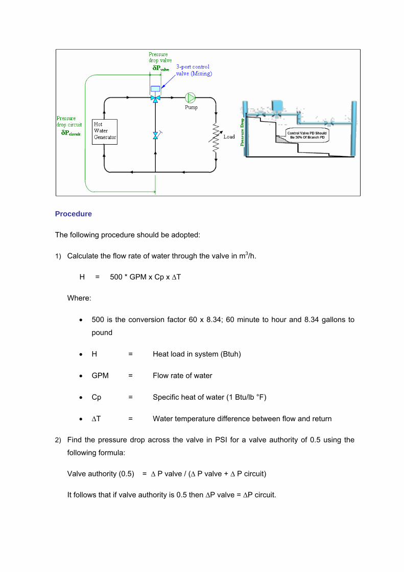
Procedure
The following procedure should be adopted:
1) Calculate the flow rate of water through the valve in m3/h.
H = 500 * GPM x Cp x ∆T
Where:
• 500 is the conversion factor 60 x 8.34; 60 minute to hour and 8.34 gallons to
pound
• H = Heat load in system (Btuh)
• GPM = Flow rate of water
• Cp = Specific heat of water (1 Btu/lb °F)
• ∆T = Water temperature difference between flow and return
2) Find the pressure drop across the valve in PSI for a valve authority of 0.5 using the
following formula:
Valve authority (0.5) = ∆ P valve / (∆ P valve + ∆ P circuit)
It follows that if valve authority is 0.5 then ∆P valve = ∆P circuit.
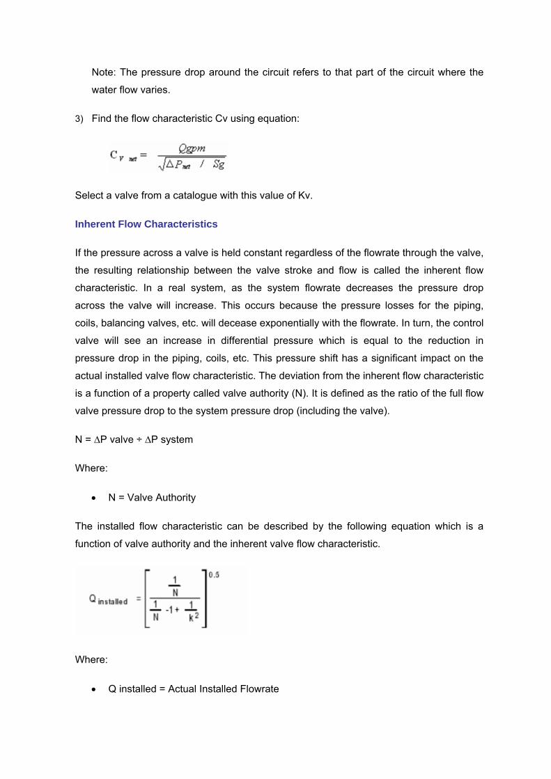
Note: The pressure drop around the circuit refers to that part of the circuit where the
water flow varies.
3) Find the flow characteristic Cv using equation:
Select a valve from a catalogue with this value of Kv.
Inherent Flow Characteristics
If the pressure across a valve is held constant regardless of the flowrate through the valve,
the resulting relationship between the valve stroke and flow is called the inherent flow
characteristic. In a real system, as the system flowrate decreases the pressure drop
across the valve will increase. This occurs because the pressure losses for the piping,
coils, balancing valves, etc. will decease exponentially with the flowrate. In turn, the control
valve will see an increase in differential pressure which is equal to the reduction in
pressure drop in the piping, coils, etc. This pressure shift has a significant impact on the
actual installed valve flow characteristic. The deviation from the inherent flow characteristic
is a function of a property called valve authority (N). It is defined as the ratio of the full flow
valve pressure drop to the system pressure drop (including the valve).
N = ∆P valve ÷ ∆P system
Where:
• N = Valve Authority
The installed flow characteristic can be described by the following equation which is a
function of valve authority and the inherent valve flow characteristic.
Where:
• Q installed = Actual Installed Flowrate
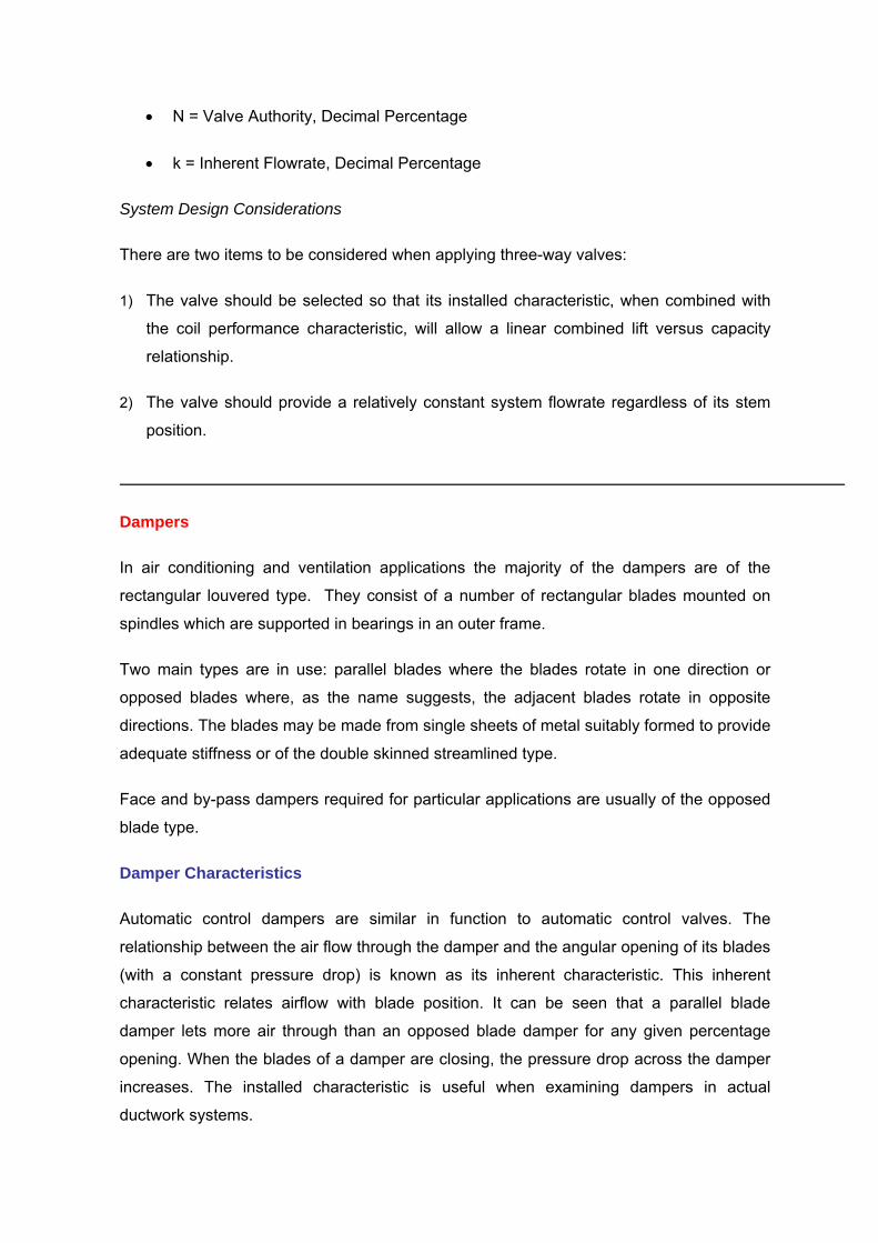
• N = Valve Authority, Decimal Percentage
• k = Inherent Flowrate, Decimal Percentage
System Design Considerations
There are two items to be considered when applying three-way valves:
1) The valve should be selected so that its installed characteristic, when combined with
the coil performance characteristic, will allow a linear combined lift versus capacity
relationship.
2) The valve should provide a relatively constant system flowrate regardless of its stem
position.
Dampers
In air conditioning and ventilation applications the majority of the dampers are of the
rectangular louvered type. They consist of a number of rectangular blades mounted on
spindles which are supported in bearings in an outer frame.
Two main types are in use: parallel blades where the blades rotate in one direction or
opposed blades where, as the name suggests, the adjacent blades rotate in opposite
directions. The blades may be made from single sheets of metal suitably formed to provide
adequate stiffness or of the double skinned streamlined type.
Face and by-pass dampers required for particular applications are usually of the opposed
blade type.
Damper Characteristics
Automatic control dampers are similar in function to automatic control valves. The
relationship between the air flow through the damper and the angular opening of its blades
(with a constant pressure drop) is known as its inherent characteristic. This inherent
characteristic relates airflow with blade position. It can be seen that a parallel blade
damper lets more air through than an opposed blade damper for any given percentage
opening. When the blades of a damper are closing, the pressure drop across the damper
increases. The installed characteristic is useful when examining dampers in actual
ductwork systems.
The pressure drop across a fully open damper depends on:
1) Damper construction
2) Blade Shape
3) Damper dimensions
4) Frame intrusion into air stream
5) Ratio of fully open damper to the duct
Typical pressure drops for fully open dampers are 10 to 15 Pa for parallel blade dampers
used in a mixing application.
The air that is being controlled can be considered an incompressible fluid at pressures
below 12 inches of water. Above that, compressibility should be considered. Gases (air)
can bend so that the volume will not be affected, and may not be controlled at all. Air can
easily stratify in duct. Therefore, a damper can be considered a poor control device at
best. At the same time, dampers can be as good as valves for control purposes, provided
they are sized properly.
Parallel Vs Opposed Blade Dampers
In HVAC installations two different types of dampers are used to modulate airflow. These
are parallel and opposed blade dampers. Each style has distinguishing characteristics
regarding fan performance control and change in air velocity profile.
Parallel blade dampers are constructed so all the blades move in the same direction and
in parallel. Parallel blade dampers tend to bend the air during the first few degrees of
rotation as they go from full open to closed, and thus do little controlling in the first 20% to
30% of movement. They bend the streams rather than modulate them. Parallel blade
dampers have an inherent curve that is not as pronounced, so the flow increases more
rapidly when the damper begins to open. Parallel blade dampers are normally used for
open-close service or fixed flow control.
Parallel blade operation is preferred:
1) When the damper makes up a significant portion of the total system pressure loss.
2) When greater control is required near the top end of the volume operating range or for
systems requiring two-position (fully open or fully closed) operation.
Note that parallel blades should not be used upstream of critical components due to
uneven airflow.
Opposed blade dampers are constructed so blades next to each other move in opposite
directions. They are normally used where the system requires airflow control and where
large amounts of stratification in the ductwork need to be prevented. Opposed blade
dampers can also be used for on/off service. Opposed blade dampers give a very slow
increase in the flow when the dampers begin to open.
Opposed blade operation is preferred:
1) When the damper doesn’t make up a significant portion of the total system pressure
loss.
2) For applications where it is necessary to maintain even distribution of air downstream
from the damper
3) For ducted outlets
4) When further opening of the opposed blades is required to obtain the same airflow
resistance as parallel blade dampers.
Some dampers are not used for control or to maintain comfort. Instead, they are used for
safety purposes. These are known as the fire and smoke dampers.
Damper Applications
Other than the volume control application for system balancing, the dampers are used for
the following:
Variable Rate Outdoor Air Introduction
Outdoor air shall be introduced by either combination motorized outdoor air/return air
mixing dampers, or a variable rate outdoor air fan controlled by CO2 sensors located in
each main return air duct. The outdoor air introduced shall be completely independent of
the point of operation of the main supply air fan.
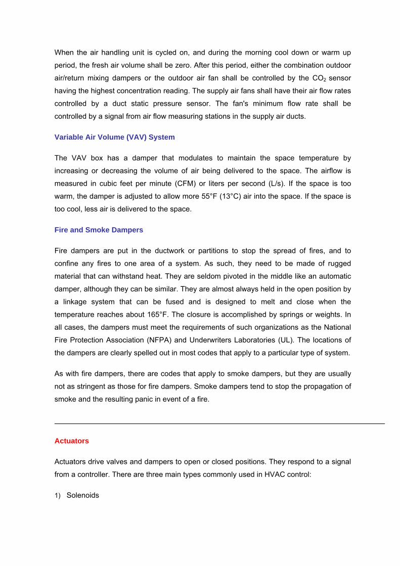
When the air handling unit is cycled on, and during the morning cool down or warm up
period, the fresh air volume shall be zero. After this period, either the combination outdoor
air/return mixing dampers or the outdoor air fan shall be controlled by the CO2 sensor
having the highest concentration reading. The supply air fans shall have their air flow rates
controlled by a duct static pressure sensor. The fan's minimum flow rate shall be
controlled by a signal from air flow measuring stations in the supply air ducts.
Variable Air Volume (VAV) System
The VAV box has a damper that modulates to maintain the space temperature by
increasing or decreasing the volume of air being delivered to the space. The airflow is
measured in cubic feet per minute (CFM) or liters per second (L/s). If the space is too
warm, the damper is adjusted to allow more 55°F (13°C) air into the space. If the space is
too cool, less air is delivered to the space.
Fire and Smoke Dampers
Fire dampers are put in the ductwork or partitions to stop the spread of fires, and to
confine any fires to one area of a system. As such, they need to be made of rugged
material that can withstand heat. They are seldom pivoted in the middle like an automatic
damper, although they can be similar. They are almost always held in the open position by
a linkage system that can be fused and is designed to melt and close when the
temperature reaches about 165°F. The closure is accomplished by springs or weights. In
all cases, the dampers must meet the requirements of such organizations as the National
Fire Protection Association (NFPA) and Underwriters Laboratories (UL). The locations of
the dampers are clearly spelled out in most codes that apply to a particular type of system.
As with fire dampers, there are codes that apply to smoke dampers, but they are usually
not as stringent as those for fire dampers. Smoke dampers tend to stop the propagation of
smoke and the resulting panic in event of a fire.
Actuators
Actuators drive valves and dampers to open or closed positions. They respond to a signal
from a controller. There are three main types commonly used in HVAC control:
1) Solenoids
2) Electric Motors
3) Pneumatic Actuators
Selection of the actuator type depends on the choice of the control system as well as
specific characteristics. The actuator characteristics that are of importance are torque and
stroke period. Torque is the ability to cause movement of the controlled device. Stroke
period is the period of movement between the limiting positions (open to closed and visa
versa). The actuator is part of the controlled device which also includes the actual valve or
damper.
Pumps & Fans Control
The control action on these devices can be simple on/off control or capacity variation if
these devices are provided with speed control variable frequency drive.
Chilled water systems are designed to supply the maximum demand of the system in
which they are installed. However, most often the HVAC is run on part load; and therefore,
the demand for water can be much less than what the system is designed for. Typical
methods of chilled water flow control include:
1) Bypass or diversion: This is a popular method in the conventional system where part
of the liquid is diverted back to the return line without going through the cooling coil.
The system employs a 3-port valve for this service. This is the most inefficient type of
control because the pump continues to run at full capacity and only a part of the
energy utilized is useful; the rest is lost in diversion. Irrespective of the capacity
utilized, the power consumption is constant.
2) Valve throttling: In this method the 2-port valve is provided in the inlet to the cooling
coil. During lean periods, the valve is throttled to restrict the chilled water flow to the
system. This is also energy inefficient as part of the energy supplied (pressure
developed) by the pump is lost across the throttle valve.
3) Variable speed devices: In this method, the speed of the pump is varied to match the
chilled water demand to the cooling coil. A Variable Frequency Drive provides an
energy efficient solution. Whenever the flow requirement varies, the speed of the pump
can be increased or decreased automatically.
Principle of operation and control of centrifugal pumps & fans
The variation of the flow, pressure developed, and the power consumption of a pump with
speed is given by the following equations:
1) Flow = K (Speed)
2) Head = K (Speed) 2
3) Power consumption = K (Speed) 3
Varying the speed of the pump achieves considerable energy savings because of the laws
which govern the operation of all pumps; in particular that the power of the motor varies by
the cube of the speed. This is the critical factor in understanding the electrical energy
savings that can be made by using variable-speed pumps.
Variable Speed Drive (VSD) Control Strategy
VSD can be programmed to adjust motor speed based on a variety of load inputs including
temperature, pressure, flow rates, or time of day setpoints. The effect of varying the speed
with a centrifugal pump is to vary both, head and flow. In the HVAC systems there is a
requirement for flow to vary based on temperature. In this instance the VFD is controlled
by both, a temperature sensor and differential pressure. The temperature controller
actuates the control valve that regulates chilled water or hot water supply to the heat
exchanger. Also, the pressure changes in a system, as a result of opening and closing of
the control valve, provide a control signal to the VFD. Sometimes in process applications,
the temperature controller directly controls the VFD to allow flow of hot or cold liquid in the
system to increase or decrease, based on the actual temperature required by the process.
This is similar in operation to pressure control, where the flow is also the variable entity,
but a constant temperature requirement from a temperature sensor replaces that from a
pressure sensor.
The fan VSD controls in the air-handler units employ the same philosophy as pumps. The
HVAC system in this case uses variable inlet terminal boxes (VAV) at multiple zones of the
space. As the damper in the VAV boxes is throttled based on the temperature reading
from the thermostat, the pressure buildup in the duct is sensed by a pressure sensor
which alters the speed of the fan to maintain the constant duct static pressure. Note that
when applying this strategy, arrangements should be made (modulating fresh air damper
based on velocity sensor) for ensuring the minimum ventilation requirements (constant
outside air intakes) as required by codes.
CONTROLLER RESPONSES
The controller's function is to compare its input instructions (from the sensor), such as
setpoint, throttling range and action, and then produce an output signal. The way in which
the controlled device acts in response to the signal is known as the control mode or control
response. There are five basic control modes which are used either individually or in
combination.
These control responses are characterized as follows::
1) Two-position
2) Floating
3) Proportional
4) Proportional plus Integral (PI or P+I)
5) Proportional plus Integral plus Derivative (PID or P+I+D)
The above control modes may be either continuous or discontinuous.
Continuous control obtains a signal from the sensor(s) all the time and the controller is
always attempting to meet the space requirements. It is sometimes referred to as
‘modulating’ control.
Discontinuous control only operates the controlled device when certain limits have been
reached as in ‘on/off’ control mode. Floating action, Proportional action, Integral action
and Derivative action are all examples of continuous or modulating control action.
Two-Position Control
In a two-position control, the controller compares the value of an analog or variable input
with instructions and generates a digital two-position output. With this form of control the
controlled device is only able to be positioned between two extremes, that is, either to a
maximum or to a minimum or to an ‘on’ or ‘off’ position.
There are no standards for defining limits. The most common terminology used is setpoint
differential. The setpoint indicates the point where the output "pulls-in", "energizes”, or is
"true." The output changes back or "drops-out" after the input value crosses through the
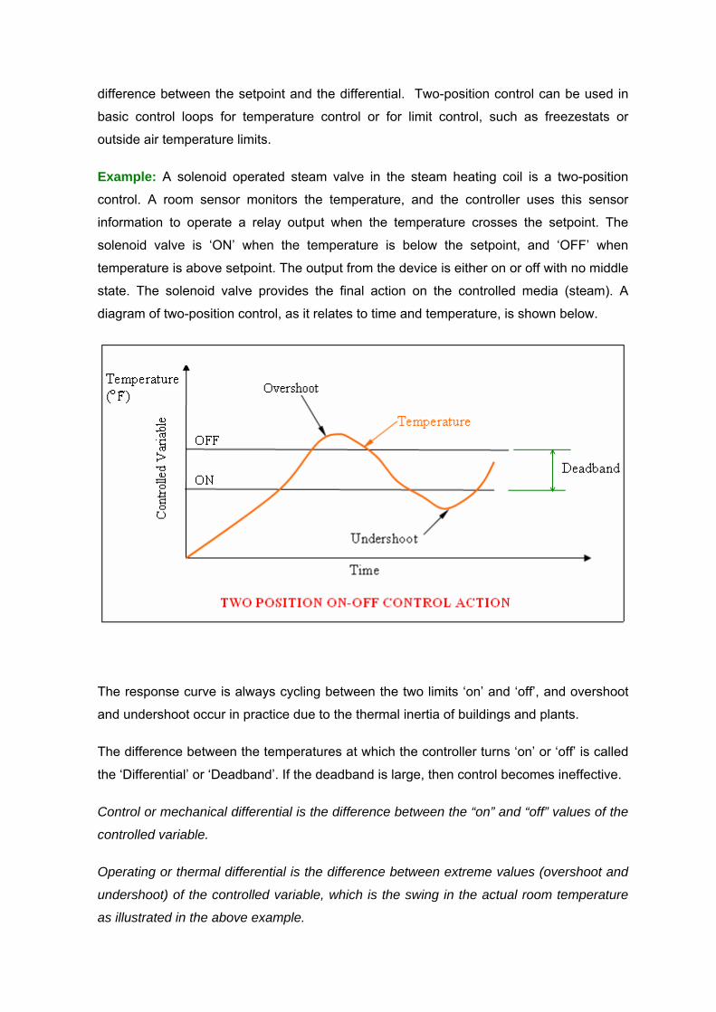
difference between the setpoint and the differential. Two-position control can be used in
basic control loops for temperature control or for limit control, such as freezestats or
outside air temperature limits.
Example: A solenoid operated steam valve in the steam heating coil is a two-position
control. A room sensor monitors the temperature, and the controller uses this sensor
information to operate a relay output when the temperature crosses the setpoint. The
solenoid valve is ‘ON’ when the temperature is below the setpoint, and ‘OFF’ when
temperature is above setpoint. The output from the device is either on or off with no middle
state. The solenoid valve provides the final action on the controlled media (steam). A
diagram of two-position control, as it relates to time and temperature, is shown below.
The response curve is always cycling between the two limits ‘on’ and ‘off’, and overshoot
and undershoot occur in practice due to the thermal inertia of buildings and plants.
The difference between the temperatures at which the controller turns ‘on’ or ‘off’ is called
the ‘Differential’ or ‘Deadband’. If the deadband is large, then control becomes ineffective.
Control or mechanical differential is the difference between the “on” and “off” values of the
controlled variable.
Operating or thermal differential is the difference between extreme values (overshoot and
undershoot) of the controlled variable, which is the swing in the actual room temperature
as illustrated in the above example.
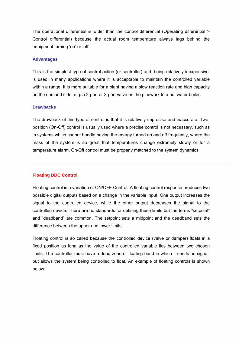
The operational differential is wider than the control differential (Operating differential >
Control differential) because the actual room temperature always lags behind the
equipment turning ‘on’ or ‘off’.
Advantages
This is the simplest type of control action (or controller) and, being relatively inexpensive,
is used in many applications where it is acceptable to maintain the controlled variable
within a range. It is more suitable for a plant having a slow reaction rate and high capacity
on the demand side; e.g. a 2-port or 3-port valve on the pipework to a hot water boiler.
Drawbacks
The drawback of this type of control is that it is relatively imprecise and inaccurate. Two-
position (On-Off) control is usually used where a precise control is not necessary, such as
in systems which cannot handle having the energy turned on and off frequently, where the
mass of the system is so great that temperatures change extremely slowly or for a
temperature alarm. On/Off control must be properly matched to the system dynamics.
Floating DDC Control
Floating control is a variation of ON/OFF Control. A floating control response produces two
possible digital outputs based on a change in the variable input. One output increases the
signal to the controlled device, while the other output decreases the signal to the
controlled device. There are no standards for defining these limits but the terms “setpoint”
and “deadband” are common. The setpoint sets a midpoint and the deadband sets the
difference between the upper and lower limits.
Floating control is so called because the controlled device (valve or damper) floats in a
fixed position as long as the value of the controlled variable lies between two chosen
limits. The controller must have a dead zone or floating band in which it sends no signal,
but allows the system being controlled to float. An example of floating controls is shown
below:
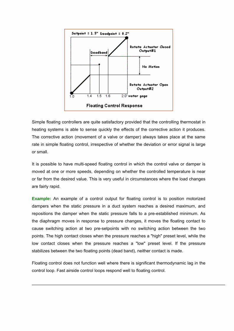
Simple floating controllers are quite satisfactory provided that the controlling thermostat in
heating systems is able to sense quickly the effects of the corrective action it produces.
The corrective action (movement of a valve or damper) always takes place at the same
rate in simple floating control, irrespective of whether the deviation or error signal is large
or small.
It is possible to have multi-speed floating control in which the control valve or damper is
moved at one or more speeds, depending on whether the controlled temperature is near
or far from the desired value. This is very useful in circumstances where the load changes
are fairly rapid.
Example: An example of a control output for floating control is to position motorized
dampers when the static pressure in a duct system reaches a desired maximum, and
repositions the damper when the static pressure falls to a pre-established minimum. As
the diaphragm moves in response to pressure changes, it moves the floating contact to
cause switching action at two pre-setpoints with no switching action between the two
points. The high contact closes when the pressure reaches a "high" preset level, while the
low contact closes when the pressure reaches a "low" preset level. If the pressure
stabilizes between the two floating points (dead band), neither contact is made.
Floating control does not function well where there is significant thermodynamic lag in the
control loop. Fast airside control loops respond well to floating control.
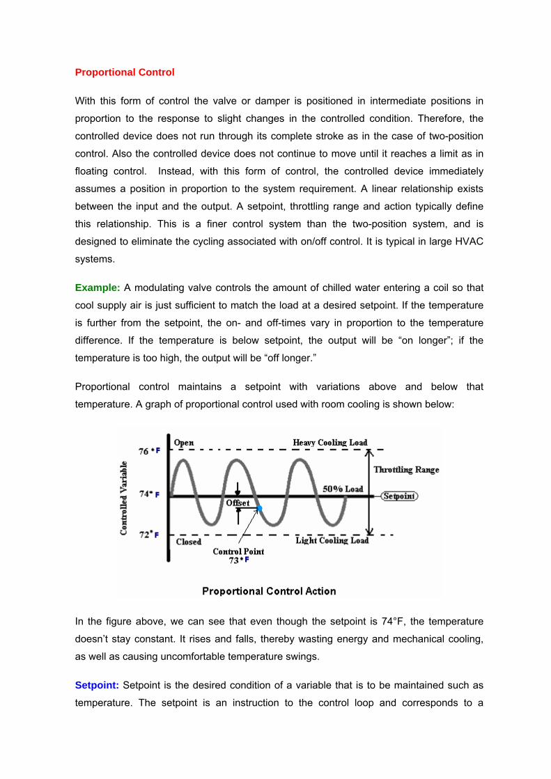
Proportional Control
With this form of control the valve or damper is positioned in intermediate positions in
proportion to the response to slight changes in the controlled condition. Therefore, the
controlled device does not run through its complete stroke as in the case of two-position
control. Also the controlled device does not continue to move until it reaches a limit as in
floating control. Instead, with this form of control, the controlled device immediately
assumes a position in proportion to the system requirement. A linear relationship exists
between the input and the output. A setpoint, throttling range and action typically define
this relationship. This is a finer control system than the two-position system, and is
designed to eliminate the cycling associated with on/off control. It is typical in large HVAC
systems.
Example: A modulating valve controls the amount of chilled water entering a coil so that
cool supply air is just sufficient to match the load at a desired setpoint. If the temperature
is further from the setpoint, the on- and off-times vary in proportion to the temperature
difference. If the temperature is below setpoint, the output will be “on longer”; if the
temperature is too high, the output will be “off longer.”
Proportional control maintains a setpoint with variations above and below that
temperature. A graph of proportional control used with room cooling is shown below:
In the figure above, we can see that even though the setpoint is 74°F, the temperature
doesn’t stay constant. It rises and falls, thereby wasting energy and mechanical cooling,
as well as causing uncomfortable temperature swings.
Setpoint: Setpoint is the desired condition of a variable that is to be maintained such as
temperature. The setpoint is an instruction to the control loop and corresponds to a
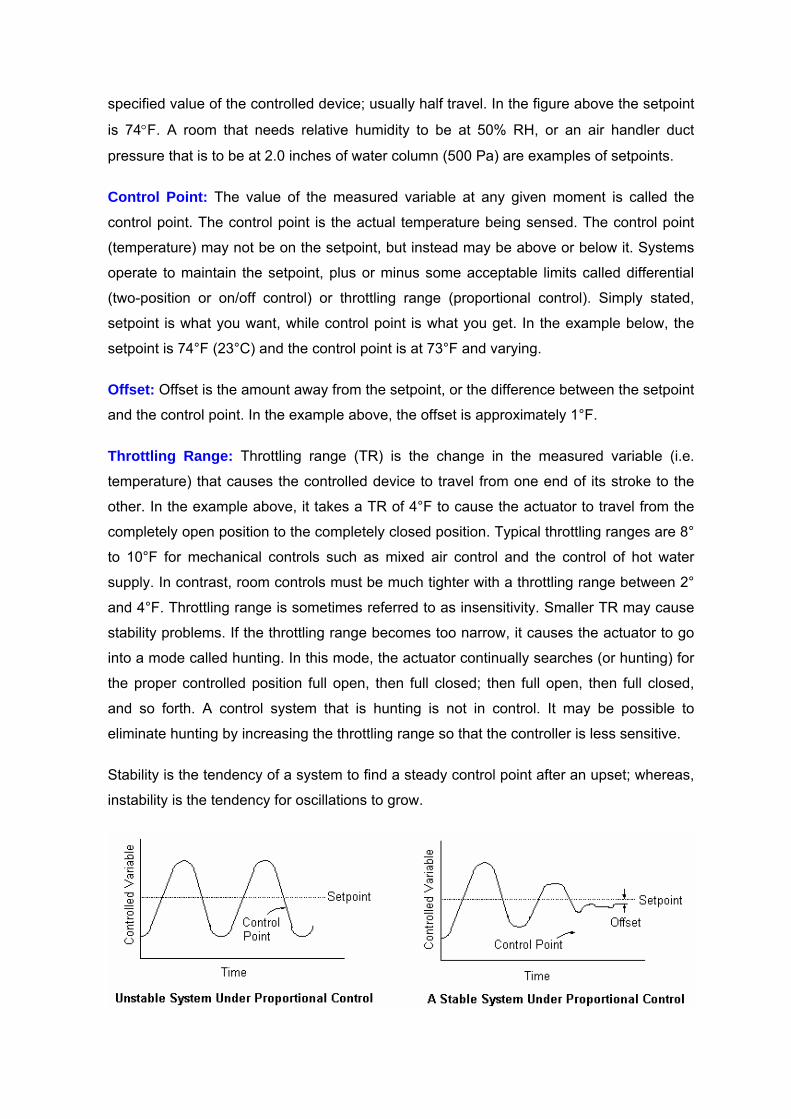
specified value of the controlled device; usually half travel. In the figure above the setpoint
is 74°F. A room that needs relative humidity to be at 50% RH, or an air handler duct
pressure that is to be at 2.0 inches of water column (500 Pa) are examples of setpoints.
Control Point: The value of the measured variable at any given moment is called the
control point. The control point is the actual temperature being sensed. The control point
(temperature) may not be on the setpoint, but instead may be above or below it. Systems
operate to maintain the setpoint, plus or minus some acceptable limits called differential
(two-position or on/off control) or throttling range (proportional control). Simply stated,
setpoint is what you want, while control point is what you get. In the example below, the
setpoint is 74°F (23°C) and the control point is at 73°F and varying.
Offset: Offset is the amount away from the setpoint, or the difference between the setpoint
and the control point. In the example above, the offset is approximately 1°F.
Throttling Range: Throttling range (TR) is the change in the measured variable (i.e.
temperature) that causes the controlled device to travel from one end of its stroke to the
other. In the example above, it takes a TR of 4°F to cause the actuator to travel from the
completely open position to the completely closed position. Typical throttling ranges are 8°
to 10°F for mechanical controls such as mixed air control and the control of hot water
supply. In contrast, room controls must be much tighter with a throttling range between 2°
and 4°F. Throttling range is sometimes referred to as insensitivity. Smaller TR may cause
stability problems. If the throttling range becomes too narrow, it causes the actuator to go
into a mode called hunting. In this mode, the actuator continually searches (or hunting) for
the proper controlled position full open, then full closed; then full open, then full closed,
and so forth. A control system that is hunting is not in control. It may be possible to
eliminate hunting by increasing the throttling range so that the controller is less sensitive.
Stability is the tendency of a system to find a steady control point after an upset; whereas,
instability is the tendency for oscillations to grow.
In proportional control, the control action is proportional to the deviation Q, where Q is
equal to the difference between the setpoint and the measured value. When the measured
value is higher than the set value, the deviation Q will be positive and the correcting signal
will be negative, and vice versa. Mathematically this can be written as:
Y = -kp Q
The problem with this type of control is that it will give rise to output offset; i.e. constant
error between set value and the output value. One way to reduce the offset is to reduce
the throttling range. Reducing the throttling range too far will lead to instability. The quicker
the sensor feels the control response, the larger the throttling range has to be to produce
stable control. Also the value of kp should be chosen in such a way that it makes the
system response faster as well as it should not affect the stability of the system.
Facts about Proportional Control
1) The proportioning action occurs within a “proportional band” around the setpoint.
Outside this band, the controller functions as an on/off unit with the output either fully
on (below the band) or fully off (above the band). At the setpoint (the midpoint of the
proportional band), the output “on:off” ratio is 1:1; that is the ‘on-time’ and ‘off-time’ are
equal.
2) In proportional control, a unique value of the measured variable corresponds to full
travel of the controlled device and another unique value corresponds to zero travel on
the controlled device. The change in the measured variable that causes the controlled
device to move from fully closed to fully open is called the throttling range.
3) The type of action dictates the slope of the control response. In direct-acting
proportional control response, the output will rise with an increase in the measured
variable. In a reverse-acting response, the output will decrease as the measured
variable increases.
4) In summary:
• Setpoint is a desired value.
• Control point is actual value.
• Setpoint - control point = Error or Offset
Integral Control Action
Integral control is seldom used alone. It is usually an important addition to other forms of
control, particularly to the proportional mode.
With Integral action there is continuous movement of the valve or damper when the sensor
is giving a value above or below the set-point. While deviation form the set-point exists,
the controller will get the actuator to move at a speed which corresponds to the amount of
deviation from the setpoint. In other words, the rate of movement is a function of the
amount of deviation from the set-point.
Proportional plus Integral (PI) Control
Proportional plus integral (PI) control is sometimes referred to as proportional with reset
and is designed to eliminate the offset. The controller always tries to match the setpoint
and every time the load changes, the controller attempts to make the setpoint and the
control point the same. PI control measures the offset or error over time. The error is
integrated and a final adjustment is made to the output signal from a proportional part of
this model. PI control response will work the control loop to reduce the offset to zero.
In integral control, the control action is taken proportional to the integral of deviation Q.
Mathematically this can be written as:
Y = -ki Qdt
Where,
• -ki is an integral gain constant and
• Y is the PI controller output.
Example: This approach would be applied, for example, to space temperature control in
circumstances where the load fluctuates widely over relatively short periods of time. This
could not be achieved by proportional control alone since the proportional band would
have to be too wide. Also PI control is used more generally for applications where close
control is required.
Other examples of PI control in buildings include mixed-air control, duct static pressure
control, and coil controls. Assume that the room that is being controlled has an oversized
valve. While there is no substitute for a properly sized valve, integral control can make this
condition less objectionable. To stop the actuator/valve assembly from hunting, a wide
throttling range of 8°F (4°C) may be set. However, room temperature swings of 8°F (4°C)
are typically unacceptable and complaints may become commonplace. A way to correct
this situation is perhaps to use proportional plus integral or PI control.
Advantages
The main advantage of this type of control is that the offset can be reduced.
A well set-up PI control loop will operate in a narrow band close to the setpoint and not
over the entire throttling range.
Limitations
PI control loops do not perform well when setpoints are dynamic, sudden load changes
occur, or the throttling range is small.
Derivative Control Action
Derivative control involves a further development of integral action such that the controller
output is a function of the rate of change of the controlled variable. This form of control,
like integral mode, would not normally be used alone but in combination with others.
Proportional plus Integral plus Derivative (PID) Control
Proportional plus integral plus derivative (PID) control adds a predictive element to the
control response, which takes care of sudden changes in deviation due to disturbances; or
in other words PID control speeds up action of PI control. This controller combines
proportional control with two additional adjustments which help the unit automatically
compensate for changes in the system.
PID is a precision process control application and is recommended in systems where the
load changes often and the controller is expected to compensate automatically due to
frequent changes in setpoint, the amount of energy available, or the mass to be controlled.
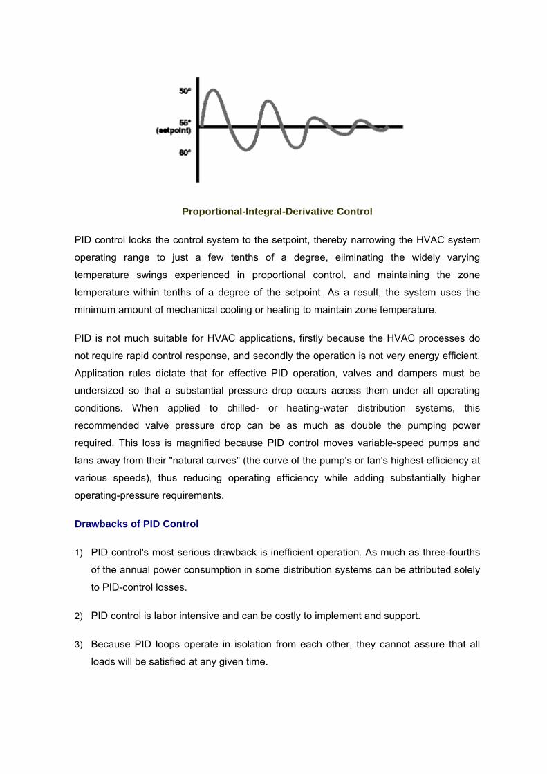
Proportional-Integral-Derivative Control
PID control locks the control system to the setpoint, thereby narrowing the HVAC system
operating range to just a few tenths of a degree, eliminating the widely varying
temperature swings experienced in proportional control, and maintaining the zone
temperature within tenths of a degree of the setpoint. As a result, the system uses the
minimum amount of mechanical cooling or heating to maintain zone temperature.
PID is not much suitable for HVAC applications, firstly because the HVAC processes do
not require rapid control response, and secondly the operation is not very energy efficient.
Application rules dictate that for effective PID operation, valves and dampers must be
undersized so that a substantial pressure drop occurs across them under all operating
conditions. When applied to chilled- or heating-water distribution systems, this
recommended valve pressure drop can be as much as double the pumping power
required. This loss is magnified because PID control moves variable-speed pumps and
fans away from their "natural curves" (the curve of the pump's or fan's highest efficiency at
various speeds), thus reducing operating efficiency while adding substantially higher
operating-pressure requirements.
Drawbacks of PID Control
1) PID control's most serious drawback is inefficient operation. As much as three-fourths
of the annual power consumption in some distribution systems can be attributed solely
to PID-control losses.
2) PID control is labor intensive and can be costly to implement and support.
3) Because PID loops operate in isolation from each other, they cannot assure that all
loads will be satisfied at any given time.
4) The goal for any distribution system employing PID control is to have a constant
pressure differential across the supply and return headers at each load, as flow in the
system changes. To accomplish this, designer’s often-oversize distribution mains or
employ reverse return-piping configurations. These pressure-leveling techniques add
costs.
5) PID control requires frequent valve- and damper-position readjustment (1- to 5-sec
reposition intervals often are recommended). This nearly continuous repositioning
shortens the actuator life, adds to maintenance costs, and makes control stability an
ongoing issue.
Stability of the System
Stability of a control system is concerned with its response to a disturbance. The system
must return to a steady state condition to be considered stable. An ‘Unstable’ system is
characterized by an oscillating response, or an ever increasing (or decreasing) response
until some natural limit is achieved.
An unstable system will often display a hunting behavior whereby the control valve is
constantly varying. (In an HVAC system, the controlled device should not change more
than 20% in a 10-minute period). This produces excessive wear on the valves and
actuators; produces thermal cycling that may impact other equipment, structure, and
contents of the building; or produces instabilities in other parts of the system.
Factors contributing to an unstable system include:
1) Too much gain (too narrow a throttling range) for a proportional system.
2) The controlled variable has too much capacity to be reasonably controlled.
3) Lack of sufficient feedback to allow control (an open loop system).
4) Control mode is too simple (ON/OFF for example).
5) Incorrect install – Often, the sensor providing feedback is located in a remote location.
Several sensors or even tens or hundreds of sensors may be wired back to an I/O
panel and several sensors may be miss-wired.
6) Too much lag time (delay) in the response of the system.
Tuning the System
Initial tuning method:
1) Verify that the system components function correctly under manual control.
a) Verify the appropriate installation of sensors and equipment.
b) Verify the wiring runs are correct.
c) Verify that the safety controls are in place and that fail-safe operation is achievable.
d) Test the system under manual control to verify predictive behavior.
2) Initial starting options of a control system:
a) Proportional Control: Start with low gain, i.e. very large throttling range.
b) Integral Control: Start with a very long integrating time.
c) Derivative Control: Start with a very short derivative action time.
3) The system should not require the controlled device to operate at an extreme position
as this is an indication of lost control.
4) Tune only one system at a time; either heating or cooling. Do not try to tune both at
the same time.
Self-Tuning and Artificial Intelligence
Tuning is a time consuming and difficult process. Several new applications have helped to
improve this process:
1) Auto-tuning – Newer Building Management Systems (BMS) have this software feature
available.
2) Adaptive Techniques – A BMS may be able to recognize changing conditions and
choose different control settings based on the sensed condition. This is helpful for
seasonal and operational changes.
3) Fuzzy Logic Control – The system monitors many inputs and performs a pseudo-logic
operation on this data. Instead of having on/off, yes/no, true/false conditions; the
sensed parameters can have degrees of on, yes, or true. Based on the combination of
these various states, the system can assign a ‘degree of control’ on a particular
device.
4) Neural Network – A control system that attempts to ‘recognize’ a given set of
circumstances that it has seen before. Therefore, it is necessary to ‘teach’ the system
how to react to given scenarios. The system attempts to choose the most likely desired
response based on a series of conditions. As the system performs, it is continuously
adjusting its decision criteria. The process is mimicking the process used by the
human brain.
In summary:
On/Off control operates with the plant fully on or fully off, which results in the controlled
temperature overshooting the differential due to the system and controller responses,
especially at low loads.
A better form of control is to vary or modulate the plant output so that as the temperature
approaches the required value, the output can be reduced to stop any overshoot. This
can be done only if the plant can be modulated; for instance, by using a modulating control
valve or, in the case of a boiler, by having a modulating burner. All of this adds to the
expense of the plant but produces better control. The control system which can provide
the modulating or varying action is proportional plus integral plus differential (PID) control.
As there are three distinct parts to PID control, it is also referred to as the three-term
control. It is possible to use only proportional or proportional plus integral control but for
computer controlled systems, like Building Management Systems (BMS), PID three-term
direct digital control is used.
The rule of thumb is that if the process has the potential to change quickly (<1 sec), use
PID or else use PI. PI is enough in many types of applications, and in some, P alone is
enough. Even if you buy equipment with a built in PID controller, you can always switch off
‘I’ and ‘D’ if needed.
DDC HVAC Systems
The modern buildings and associated HVAC design rely on a direct digital control (DDC)
system. In DDC, the inputs and outputs (in the form of input/output (IO) modules) send
information to and from a microprocessor. The microprocessor can be programmed to do
a specific task.
Definition
The definition published by ASHRAE states that: “DDC is microprocessor or computer-
based open or closed loop control of an output device based upon input data and a
sophisticated control algorithm, typically proportional, integral and derivative”. DDC
provides effective, sophisticated strategies for the optimum control and efficiency.
What is DDC?
Well in the simplest terms, it is a control system that uses a computer or many computers
linked together via a network that controls the infrastructure of a building. DDC control
consists of microprocessor-based controllers with the control logic performed by software.
Most systems distribute the software to remote controllers to eliminate the need for
continuous communication capability. The computer is primarily used to monitor the status
of the system, store back-up copies of the programs and record alarming and trending
functions. Complex strategies and energy management functions are readily available at
the lowest level in the system architecture. The central diagnostic capabilities are also a
significant asset.
DDC Terminology & Theory of Operation
Data, in the form of signals from input devices connected to the input terminals on the
controller, is conditioned by the input multiplexer then converted to digital values by the
analog to a digital converter prior to entering the DDC micro-processor. Digital
computations are performed on this data based on the set of instructions (program)
installed in the DDC controller. The outputs, as a result of this digital processing, are
converted to analog by the analog converter. The important terminologies for DDC
covered in this section are:
1) Points
• Digital Input (DI)
• Digital Output (DO)
• Analog Input (AI)
• Analog Output (AO)
2) Universal Points
3) Pulse Input
Points
When specifying an HVAC system, we often hear the term "point." A point is the
communications connection between a DDC Controller, sensors and controlled devices. It
is a common term used to describe data storage locations within a DDC system. Data can
come from sensors or from software calculations and logic. Data can also be sent to
controlled devices or software calculations and logic. Each data storage location has a
unique means of identification. If we check an energy management guide, a point is
defined as: "any input or output device used to control the overall or specific performance
of equipment or output devices related to equipment." DDC is essentially made up of two
types of points: inputs (or sensors) and outputs (or actions). Input refers to information
being sent to the DDC controller and output refers to signal sent out from the controller.
Inputs and outputs are further categorized as analog or digital. So in reality, there are four
different points: 1) Analog input, 2) Digital input, 3) Analog output, and 4) Digital output.
Data Types
1) A digital input (DI) monitors “status” which can be either ON or OFF. In the case of an
air handler, an airflow switch could provide the status On or Off. Other names for
digital inputs are two-position, binary, discrete, or logical. Examples of digital inputs are
occupied/unoccupied switches, flow switches, and static pressure switches
2) A digital output (DO) switches a device from one status to another or maintains a
status. If the control system is programmed to turn on an air handler at 8 a.m. and off
at 5 p.m., the digital output is the action of turning the switch on and keeping it on until
the stop time. Examples of digital outputs are electric heaters, fans, pumps, two
position valves, lighting contactors, DX cooling, supply fans, boiler enable and chiller
enable.
3) In contrast to digital signals which are either ON or OFF, analog signals can place the
equipment in a range of positions. Therefore, an analog input (AI) is a varying or
modulating signal that is sent to the controller. Other names for analog are
proportional, numerical, or modulating. An analog input is a sensor that monitors
“physical data” such as temperature, pressure, carbon dioxide or airflow
measurements. An example is a temperature sensor which is analog because it is a
proportional signal; it varies within a range of extremes. Other examples of analog
inputs are hot water temperature, room temperature, outside air temperature, zone
humidity, and building static pressure.
4) An analog output (AO) is a varying or modulating signal sent from the controller. An
analog output is the interface between a command generated by the processor and
the controlled equipment. In other words, it’s the physical action of a proportional
device; like an actuator opening an air damper from 20% to 50%. Other typical analog
outputs include modulating valve positions and variable frequency drives. Examples of
analog output include hot water valves, outside air dampers, and variable frequency
drives.
Data Flow
Data flow refers to whether the data is going into or out of the DDC component/logic. Input
points describe data used as input information and output points describe data used for
output information.
Data Source
Points can also be classified as external when the data is received from an external device
or sent to an external device. External points are sometimes referred to as hardware
points. Internal points represent data created by the logic of the control software. Other
terms used to describe these points are virtual points, numeric points, data points and
software points.
Contact types
If a controller has dry contacts, power must be added to make the relay work. If a
controller has powered contacts, then there is already power at the contacts and external
power is not wired to those terminals. Triacs are a very common type of powered contacts.
Universal Points
While reviewing the local control unit, one may learn that this air handler has 10 points or
that controller has 64 points. This indicates how many connections (points) can be made
to sensors and controlled devices. Each controller has a maximum number of each point
type. Some points have a fixed configuration while other points have universal or
adaptable, arrangements.
Fixed Point Configuration
Fixed points are those that are dedicated to be of a specific type and cannot be changed.
For example, a controller may have four analogue inputs (AIs). These AIs may not have to
be used but they are AIs only and cannot be changed to another point type.
Universal Point Arrangement
To address the problem of having fixed points that go unused, some points may be
programmed as any of the four different types: AI, AO, DI, or DO. These are referred to as
Universal Points. For example, if an additional temperature sensor (an AI) is desired, and
all that is available in a fixed configuration controller is a digital input, another controller
would be required to accommodate the sensor. By using a universal point configuration,
any point on the controller can be programmed as an AI after it has been wired. This
flexibility can be advantageous over a fixed-point configuration.
Pulse Inputs
A Pulse Input point type allows a controller to monitor the power consumption of a device
such as a chiller, fan, or an air hander. Pulse inputs are used to monitor the power
consumption of a whole building. Current transformers and transducers can also monitor
kilowatt usage but they use a 4 to 20 mA signal; so an AI point would be required.
Examples:
The above concepts are illustrated in the following two examples:
1) Consider the processor (controller) is programmed to adjust an air handler mixed air
damper based on the relative humidity level in the zone as compared to the relative
humidity outside. Each humidity sensor would act as a separate analog input,
measuring the percentage of relative humidity in the air and transmitting the
information to the processor. Consider it’s a warm but damp day, and the outside air
relative humidity sensor tells the processor that the relative humidity level of outside air
is too high. The processor then instructs the air handler’s mixed air dampers to
modulate to a lower percentage of outside air. This action is performed by an analog
output.
2) Consider the processor (controller) is programmed to switch on the air handler fan
when the space air temperature reaches 75°F. The temperature reading would still be
an analog input, but the action of turning the fan “on” is a discreet output. When an
airflow sensor in the air handler confirms that the fan is indeed on, this is a discreet
input. Once the input-output-input cycle is complete, it repeats again. The temperature
sensor measures the air temperature and sends the data to the processor. The
processor sees that it’s still 75°F and instructs the fan to stay on. The fan switch
reports back to the processor that the fan is still operating. The cycle, which repeats
continuously to keep the space at the desired temperature, is called closed loop
control.
DDC Hardware
The direct digital control loop consists of three main components: a sensor, a controller,
and a controlled device. The sensor measures the data, the controller (processor)
processes the data, and the controlled device causes an action. Sensors and controlled
devices are connected directly to the processor (computer). The controller's function is to
compare its input (from the sensor) instructions, such as setpoint, throttling range and
action, then produce an output signal. The control logic usually consists of a control
response along with other logical decisions that are unique to the specific control
application.
Operational Concept
The primary element for DDC is the digital computation unit (MPU or CPU) in the
controller. The basic components are:
1) Microprocessor
2) Memory
3) Input/Output Multiplexers
4) Analog-to-Digital (AID) & Digital-to-Analog (D/A) Converters
5) Communications Port
Closed Loop Control
This input/output control is the closed loop process. In closed loop control, the control
signal is sent from the processor to the controlled device (output) while the controlled
device sends constant feedback (input) to the processor. Within the processor, closed loop
control signals are determined by control algorithms, configuration values, time schedule
data, and setpoint schedule data.
Control algorithms are mathematical calculations required to be performed by the DDC
processor. These consist of formulas that actually compute the control signals and
maintain closed loop control. Because one control unit handles multiple inputs and
outputs, the algorithms require configuration values which are numbers that represent the
various points found in an HVAC system. The algorithms also require a time schedule and
setpoint schedule data, such as the times specific equipment should turn on and off,
temperatures at which valves and dampers should reset, and so on. Using this data, a
processor can be programmed to perform a wide range of control algorithms. Some of the
most typical are:
1) Heating/cooling coil control
2) Humidification/dehumidification
3) Mixed air damper optimization
4) VAV fan control
5) VAV supply and return fan tracking
6) Indoor air quality
7) Control point reset
8) Time of day scheduling
9) Discrete interlock
10) Discrete staging
11) Primary/secondary pump control
12) Night free cooling
13) Permissive interlock
Example:
A facility requires all the lights in the office block come on at 8 AM. This instruction shall be
programmed in the control system for execution. At 8 AM the next morning, the control
system processor sends a signal to the circuit panel for the lights to turn on, and a sensor
in the circuit panel sends a message to the processor confirming the action.
The Control Network
Sizable HVAC systems may have any number of controllers. These are networked
together through a communication bus the same way computers are networked together
to form a Local Area Network (LAN). The bus allows the user to see all the system’s inputs
and outputs (analog and discreet) and monitor their operation via a computer software
program.
Architecture
System architecture is the map or layout of the system used to describe the overall local
area network (LAN) structure. This map will show where the operator interfaces with the
system and may remotely communicate with the system. The network, or LAN, is the
media that connects multiple devices. This network media allows the devices to
communicate, share, display and print information, as well as store data. The most basic
task of the system architecture is to connect the DDC controllers so that information can
be shared between them.
Controller Classification
Controllers can be categorized by their capabilities and their methods of communication
(controller-to-controller). In general, the controllers can be categorized as high-end primary
controllers and low-level secondary controllers. The levels describe where the controller
resides within the system architecture on the control network, which is judged by the
importance of application.
Primary Controllers
Higher-end controllers normally reside on a higher-level network and communicate in a
peer-to-peer fashion. These are called primary controllers. Peer-to-peer means that the
controllers can share information to other peer-to-peer devices without going through an
intermediary device (called a supervisory interface). These primary controllers can range
in cost from $1500 to $4000 or more. These have more memory, more sophisticated
CPUs, higher resolution A/D converters, more accurate clocks and can store more
complex control strategies as well as trends, schedules, and alarms. Primary controllers
typically have the following features:
1) Real-time accurate clock function
2) Full software compliment
3) Larger total point capacity
4) Support for global strategies
5) Buffer for alarms/messages/trend & runtime data
6) Freeform programming
7) Downloadable database
8) Higher analog/digital converter resolution
9) Built-in communication interface for PC connection.
Secondary Controllers
The lower-level controllers normally reside on a lower-level polling network. These
controllers have more limited memory and processing capabilities and must use a
supervisory interface device to communicate with all other devices. There are many
different designs and can cost from $100 to $1000. Some are designed for terminal
applications like variable air volume boxes or fan coil units. Others may be used for air
handling systems with simple to moderately complex sequences of operation. These
controllers have limited memories; they usually do not store historical information (such as
trends) but rely on the supervisory interface for this function. Secondary controllers
typically have the following features:
1) Not necessarily 100% stand-alone
2) Limited software compliment
3) Smaller total point count
4) Freeform or application specific software
5) Typically lower analog-to-digital converter resolution
6) Trend data not typically stored at this level
7) Typical application is terminal equipment or small central station equipment.
LAN Communication
The controllers and all devices on a network communication system can be characterized
as peer-to-peer or polling.
The controllers on the peer-to-peer LAN may be primary controllers, secondary controllers,
or a mix of both.
In a polling controller LAN, the individual controllers cannot pass information directly to
one of the other controllers. Instead, data flows from one controller to the interface and
then from the interface to the other controller. The interface device manages
communication between the polling LAN controllers and with higher levels in the system
architecture. It may also supplement the capability of polling LAN controllers by providing
the following functions: clock functions; buffer for trend data, alarms or messages; and
higher order software support.
Communication Interface
The communications interface defines the path between devices that do not use the same
communications protocol. This includes computers, modems and printers.
Many systems combine the communications of a peer-to-peer network with a polling
network. The polling LAN-based devices can receive data from the peer-to-peer devices
but data must flow through the interface.
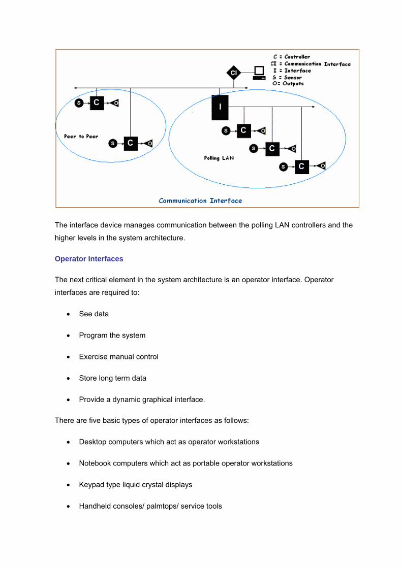
The interface device manages communication between the polling LAN controllers and the
higher levels in the system architecture.
Operator Interfaces
The next critical element in the system architecture is an operator interface. Operator
interfaces are required to:
• See data
• Program the system
• Exercise manual control
• Store long term data
• Provide a dynamic graphical interface.
There are five basic types of operator interfaces as follows:
• Desktop computers which act as operator workstations
• Notebook computers which act as portable operator workstations
• Keypad type liquid crystal displays
• Handheld consoles/ palmtops/ service tools
• Smart thermostats
Desktop computers are centralized operator workstations where the main function is
programming; building and visualizing system graphics; long term data collection; and
alarm and message filtering.
Notebook computers may connect to the LAN through a communication interface that
stands alone or is built into another device. The notebook computer connected to the LAN
at a particular level may not have the same capability as a computer connected to the LAN
at a higher level.
Keypad liquid crystal displays typically are limited to point monitoring and control. They
may have some limited programming capability such as changing a setpoint or time
schedule.
Handheld consoles, palmtops and service tools are proprietary devices that connect to
primary controllers or secondary controllers. Typically they allow point monitoring and
control, controller configurations (addressing and communication set-up), and calibration
of inputs and outputs.
Smart thermostats are sensors with additional capabilities. They connect to secondary
controllers and have a service mode to allow for point monitoring, control and calibration.
They also have a user mode that allows point information to be displayed, setpoint
adjustment and an override mode.
Protocols
In the DDC use, there are three classifications of protocols: closed protocol, open protocol
and standard protocol. A closed protocol is a proprietary protocol used by a specific
equipment manufacturer. An open protocol system uses a protocol available to anyone,
but not published by a standards organization. A standard protocol system uses a protocol
available to anyone. It is created by a standards organization. An open system is defined
as a system that allows components from different manufacturers to co-exist on the same
network. These components would not need a gateway to communicate with one another
and would not require a manufacturer specific workstation to visualize data. This would
allow more than one vendor’s product to meet a specific application requirement.
The sole use of an open or standard protocol does not guarantee that a DDC system will
be an open system. A manufacturer has the ability to use open or standard protocols, yet
create a closed system, thus continuing a building owner’s dependence on a single
manufacturer. This can be accomplished by using unique communication speeds, unique
data formatting and by not adopting the full range of an open protocol.
Note: A building owner/engineer should thoroughly research a manufacturer’s claim of an
open system. Different systems may not be compatible with one another.
BACnet™ communication protocol
In some cases it may be desirable and beneficial to connect different vendors DDC field
panels together to perform supervisory monitoring, management and control functions.
The Building Automation and Control Networking (BACnet™) protocol provides a means
to interconnect different manufacturers’ control equipment.
BACnet™ is a communication protocol specification. The development of this specification
was prompted by the desire of the building owners and operators for cost-effective inter-
operability; i.e., the ability to integrate equipment from different vendors into a coherent
automation and control system.
Work on the BACnet™ specification began in June 1987 and was completed and
approved by the ASHRAE standards committee in June 1995, and by the American
National Standards Institute in December 1995. Although the specification is complete,
work is not yet completed on a specification for a methodology for conformance testing of
products claimed by vendors to be BACnet™ compatible.
BACnet™ is intended as a standard communications protocol for HVAC&R. It is not
directly intended for other building services such as lighting, fire and security although it
does not preclude integrating these functions into a common system.
BACnet™ is a mechanism that conveys information including, but not limited to:
a) Hardware binary I/O values
b) Hardware analog I/O values
c) Software binary and analog I/O values
d) Schedule Information
e) Alarm and event information
f) Files
g) Control logic
To use the BACnet™ standard the specifier should”:
a) Understand the structure of the protocol
• Conformance Classes
• Devices, Objects, Services
• Architecture
b) Define inter-operability needs at each level of the system: supervisory computer,
operator interfaces, field panels, sensors/actuators.
c) Choose which devices will be capable of sending and receiving messages.
d) Define the functionality of the communicating devices (based on specifics/
definitions in the standard, conformance class and functional groups).
e) Define networking options. Be aware of the need for inter-networking devices
(LANs, routers, repeaters, segments, gateways, and bridges).
f) Obtain integration and commissioning services (from a vendor).
Building Automation Systems (Supervisory Control)
The role of a supervisory control is to integrate all functions of a building into a common
network. This networking allows the concept of "intelligent" building where a master control
computer operates everything from the elevators, lighting and HVAC systems to the
security, emergency power, and life-safety/fire protection systems. All these systems can
be programmed to operate in an integrated manner. For example, suppose there is a
smoke detector that alarms on the ninth floor. The computer might sound the fire alarm on
that floor immediately, drive all available elevators to the ground floor for fire personnel
use, open the exhaust dampers to remove smoke from that floor, and pressurize the
stairwells and adjacent floors to prevent smoke from migrating to those areas. All this
building information is transferred through a pair of twisted wires like speaker cable. The
electronic signals used in these systems are typically -5 to +5 volt direct current (VDC).
This control signal is only used to control the actuator that actually controls the device. In
other words, this voltage is used to set a pneumatic or electrical signal that actually does
the work. DDC computer systems are sensitive to high voltage transients such as lightning
and current inrush when motors are started, and must be protected from these signals with
varisters. Supervisory control systems have many names such as BAS (Building
automation system), BMS (Building management system), EMCS (Energy monitoring and
control system), FMS (Facility management system) and EMS (Energy management
system). BAS is the most generic of these terms.
For more information on the subject refer to the ASHRAE journals.
Advantages of Using DDC
The benefit of direct digital control over past control technologies (pneumatic or distributed
electronic) is that it improves the control effectiveness and increases the control efficiency.
DDC systems for HVAC have many advantages as follows:
1) Speed - Signals can be sent instantly.
2) Complex calculations - The computer can work out many complex calculations that a
technician might not be able to do because of the time required.
3) Reliability - The computer always works a problem in the same way, so it is reliable
and accurate as long as the information fed to it is accurate.
4) Central monitoring and control - A whole system can be controlled from a single
location. This allows instant operator interaction with the building's system or many
systems. It can provide a picture of "what is going" on in the building via a computer
screen. It can also change system operation from the same central location. This could
include opening/closing valves, starting/stopping fans and changing setpoints to name
a few.
5) Complex adjustments - A computerized control system receives signals from all the
sensors in the system and processes all the information at the same time. It instantly
computes the best possible settings for the entire system and outputs many different
signals continuously to control the system. In a non-computerized system, each
controller reacts to only one or two conditions rather than to the needs of the whole
system.
6) Anticipation - A computerized control system anticipates what will be needed. For
example, if the outside air temperature is extremely hot or cold, system settings will
adjust for the additional time it will take to bring the space to the desired setpoint. It will
also anticipate needs when the outside air temperature is changing rapidly.
7) Printed reports - A computerized system may generate all types of reports and graphs
to show trends of the system. These can be printed as desired.
8) Improved accuracy - There is less chance of human error. Equipment is more accurate
because there are no mechanical devices and no mass (weight) such as moving
contact points or mercury bulb in the computer Automatic alarms.
9) More precise control - There is less time lag between setpoints and activation. DDC
systems are electronic and use electronic circuits and devices for monitoring and
control. Compared to a pneumatic sensor which is ± 2°F accurate, a DDC sensor is
±0.3°F. As a result, improved comfort and IAQ are achieved by monitoring conditions
close to a constant level.
10) Conservation of energy - Tighter control of the system. The hours of occupation can be
refined and the temperature in the space remains at a more constant level. In some
duct systems this means that many alternate heating and cooling cycles are
eliminated. Strategies such as demand monitoring and limiting can be easily
implemented with DDC systems. The overall demand for a facility can be monitored
and controlled by resetting various setpoints based on different demand levels. By
storing trends, energy consumption patterns can be monitored.
11) Sequencing - Provides the proper sequence of equipment start-up after a system shut-
down or a power failure.
12) Feedback - Not only sends control signals to the operating systems but also feeds
back and records data concerning the status, environmental conditions, and
mechanical conditions. This data can be printed as reports, charts, or graphs.
13) Innovation - Allows the operator to invent additional strategies that can be carried out
by a computerized system.
14) Flexibility - Since the logic of a control loop is in the software, this logic can be readily
changed. In this sense, DDC is far more flexible in changing reset schedules, setpoints
and the overall control logic. Users are apt to apply more complex strategies,
implement energy saving features and optimize their system performance since there
is less cost associated with these changes than there would be when the logic is
distributed to individual components.
15) Operation & Maintenance - The alarming capabilities are strong and most systems
alarm to various locations on a given network. The trending capability technician or
engineer to troubleshoot system and control problems is visualized in various formats.
This data can also be stored and measure equipments' performance over time. Run-
times of various equipment alarms/messages can be generated when a lead/lag
changeover occurs or if it is time to conduct routine maintenance.
ENERGY SAVING FEATURES
The annual running cost of a building's heating, lighting and electrical power system can
be quite significant and can result in high overheads in any business. The energy
conservation has become important in the design of buildings.
Time Control & Energy Saving Devices
The best energy conservation method is to ensure that the energy is only used during the
time periods it is required. In heavyweight buildings it may take some time to build up room
temperatures when starting the heating system from cold, so the time clock may be set to
bring the heating on several hours before the occupancy period. Also the heating can be
set to go off some time earlier than when the occupants leave the building. There are two
types of time clocks used in controls:
1) The small synchronous motor following 60Hz, with or without clockwork 'spring'
reserve mechanism.
2) Digital clocks driven by electronic oscillator and quartz crystal regulated. They may
have a battery backup to cover mains failure.
These can give several independent switched circuits their own programs. The figure
below shows a wiring diagram with timed control.
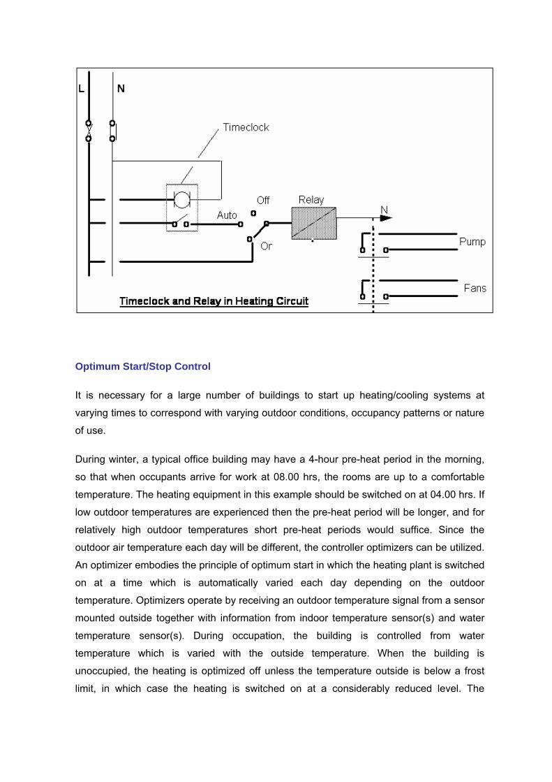
Optimum Start/Stop Control
It is necessary for a large number of buildings to start up heating/cooling systems at
varying times to correspond with varying outdoor conditions, occupancy patterns or nature
of use.
During winter, a typical office building may have a 4-hour pre-heat period in the morning,
so that when occupants arrive for work at 08.00 hrs, the rooms are up to a comfortable
temperature. The heating equipment in this example should be switched on at 04.00 hrs. If
low outdoor temperatures are experienced then the pre-heat period will be longer, and for
relatively high outdoor temperatures short pre-heat periods would suffice. Since the
outdoor air temperature each day will be different, the controller optimizers can be utilized.
An optimizer embodies the principle of optimum start in which the heating plant is switched
on at a time which is automatically varied each day depending on the outdoor
temperature. Optimizers operate by receiving an outdoor temperature signal from a sensor
mounted outside together with information from indoor temperature sensor(s) and water
temperature sensor(s). During occupation, the building is controlled from water
temperature which is varied with the outside temperature. When the building is
unoccupied, the heating is optimized off unless the temperature outside is below a frost
limit, in which case the heating is switched on at a considerably reduced level. The
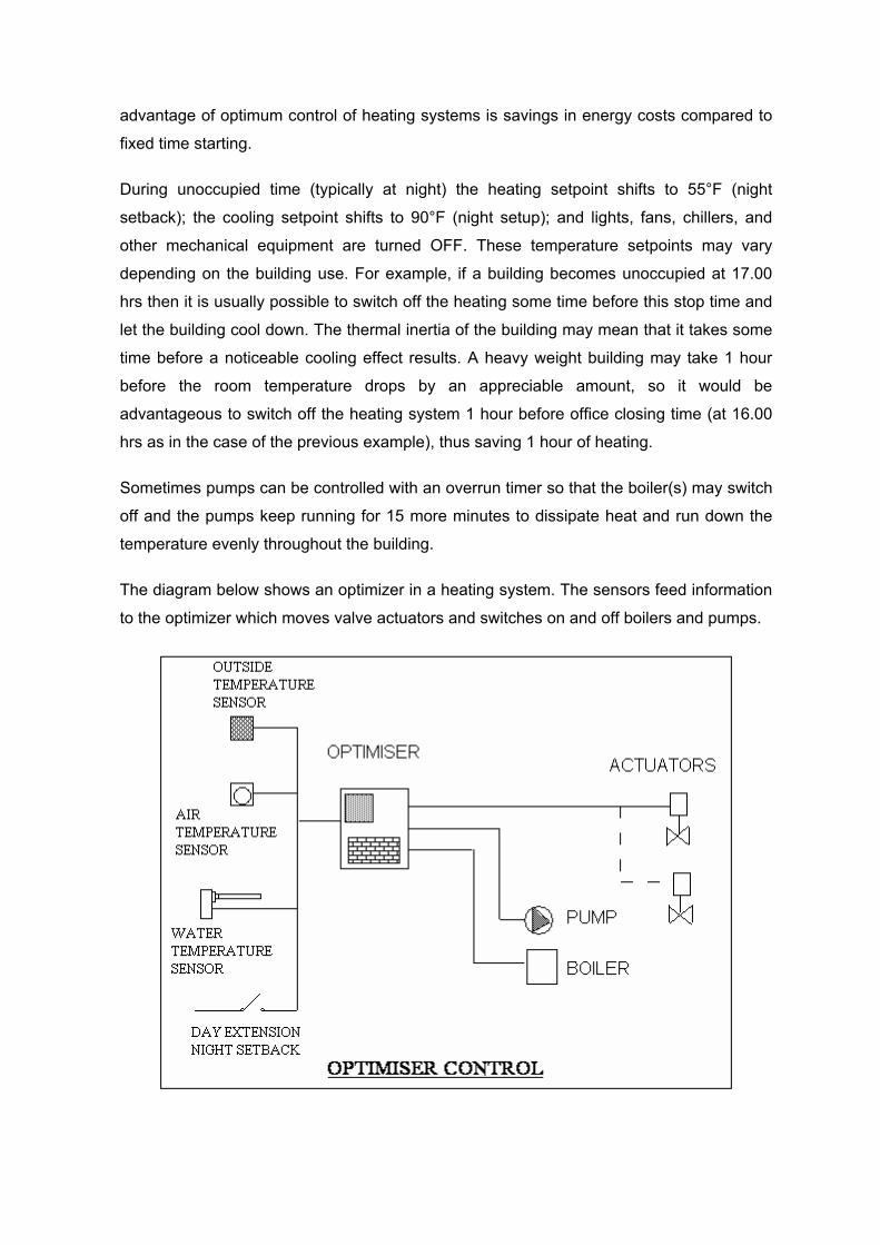
advantage of optimum control of heating systems is savings in energy costs compared to
fixed time starting.
During unoccupied time (typically at night) the heating setpoint shifts to 55°F (night
setback); the cooling setpoint shifts to 90°F (night setup); and lights, fans, chillers, and
other mechanical equipment are turned OFF. These temperature setpoints may vary
depending on the building use. For example, if a building becomes unoccupied at 17.00
hrs then it is usually possible to switch off the heating some time before this stop time and
let the building cool down. The thermal inertia of the building may mean that it takes some
time before a noticeable cooling effect results. A heavy weight building may take 1 hour
before the room temperature drops by an appreciable amount, so it would be
advantageous to switch off the heating system 1 hour before office closing time (at 16.00
hrs as in the case of the previous example), thus saving 1 hour of heating.
Sometimes pumps can be controlled with an overrun timer so that the boiler(s) may switch
off and the pumps keep running for 15 more minutes to dissipate heat and run down the
temperature evenly throughout the building.
The diagram below shows an optimizer in a heating system. The sensors feed information
to the optimizer which moves valve actuators and switches on and off boilers and pumps.
Duty Cycling
Duty cycling is a strategy that cycles certain loads (such as small exhaust fans) on and of.
For example, exhaust fans may be cycled “on” for 20 minutes and then shut “off” for 10
minutes continuously throughout the occupied time. This is referred to as a fixed duty
cycle. At the end of the day, the “off” time may amount to a large portion of the time.
This strategy may show huge savings annually on paper but in reality it should be applied
with caution. It may not be cost effective since the money that is saved during the OFF
time could be offset by the large current draw required for starting up the large fan.
Secondly the on and off cycles can require more maintenance on the motor belts and
other equipment.
A modification of this strategy is called the Temperature Compensated Duty Cycle. This
strategy is used with electric baseboard heaters. If the temperature in the space is 70°F
(21°C), the heaters are ‘on’ for 1 minute and ‘off’ for 14 minutes. If the space temperature
drops to 68°F (20°C), then the heaters are ‘on’ for 7 minutes and ‘off’ for 8 minutes. If the
space temperatures continue to drop to 66°F (19°C), then the heaters are ‘on’
continuously and are not shut off until the temperature in the space reaches the setpoint.
Electric Demand Limiting
Trying to manage the consumption of electricity is a concern for the utility providers as well
as the building owners. The utility providers typically impose demand charges/penalties if
the facility’s electric usage exceeds the demand’s set limit. Even one excursion beyond
the demand limit could mean 30 to 70% penalty over the electric bill. An effective way to
manage this, demands the use of an Electric Demand Limiting (EDL) program that
computes the magnitude of the demand and automatically sheds sufficient loads (usually
non-critical loads) to prevent the demand exceeding the set limits. Once the demand drops
below the limit, those previously shed loads are brought back on line.
Enthalpy Optimization
During the cooling season, additional energy savings may be realized by choosing the air
source (either return air or outside air) which contains the least amount of total heat
(Enthalpy). Enthalpy is determined by a combination of temperature and relative humidity.
In a nutshell, during night times when the outdoor ambient air conditions are more
favorable, less of return air and more of outside air will be drawn. There are energy
savings if the cooling coil is presented with the air having the lower enthalpy whether this
is return air or outside air.
Night Purge Cycle
During the cooling season, if the inside temperature is considerably greater than the
outside air temperature, then the air handling units may be turned ON during the night to
purge the warm air out of the building. This is called a Night Purge Cycle. This type of free
cooling reduces the amount of mechanical cooling that has to take place the following
morning. However, caution should be taken concerning the humidity of the outside air. To
address this concern, an enthalpy optimization program could be established to ensure
that only the lowest enthalpy air is used to cool the building at night. Whether or not to use
the night purge cycle is determined by comparing the cost of running the air handling units
at night versus the cost of running the mechanical cooling in the morning.