Embed Size (px)
Citation preview
Humans Are Not Machines: The Behavioral Impact of Queueing
Design on Service Time
Masha Shunko† Julie Niederhoff‡ Yaroslav Rosokha§
Abstract:
Using behavioral experiments, we study the impact of queue design on worker pro-
ductivity in service systems that involve human servers. Specifically, we consider
two queue design features: queue structure, which can either be parallel queues
(multiple queues with a dedicated server per queue) or a single queue (a pooled
queue served by multiple servers); and queue-length visibility, which can provide
either full or blocked visibility. We find that 1) the single-queue structure slows
down the servers, illustrating a drawback of pooling; and 2) poor visibility of the
queue length slows down the servers; however, this effect may be mitigated, or even
reversed, by pay schemes that incentivize the servers for fast performance. We pro-
vide additional managerial insights by isolating two behavioral drivers behind these
results–task interdependence and saliency of feedback.
Keywords: Behavioral Operations, Queueing Systems, Service Time, Real Effort
Experiments
† Foster School of Business, University of Washington • Email: [email protected]
‡ Whitman School of Management, Syracuse University • Email: [email protected]
§ Krannert School of Management, Purdue University • Email: [email protected]
∗This work was supported by grants from the Robert H. Brethen Operations Management Institute at the
Whitman School of Management.
1 Introduction
In service systems, managers are constantly seeking ways to improve customers’ experience by re-
ducing service waiting times. Service windows, such as those at banks, post offices, motor vehicle
offices, and delicatessens, are known for single-queue structures (a pooled queue served by mul-
tiple servers). Retail companies such as TJ Maxx, Hannaford, and Target have implemented or
experimented with a single-queue, “next available” checkout policy with varying degrees of success
(Hauss, 2008; Helms, 2011; Fantasia, 2009). Nevertheless, parallel queues are still common practice
for many service environments in which servers have face-to-face contact with customers and with
other servers (e.g., retail stores, ticket booths, security gates, fast food restaurants, etc.). Simi-
larly, direct job assignments can be found in service systems in which the servers have no direct
contact with either customers or other servers (e.g., technical support centers pre-assign tickets to
specific agents), effectively creating a parallel-queues policy, so it is critical to consider both queue
structures when studying worker productivity.
Bendoly et al. (2010) suggest that various behavioral factors impact worker productivity. They
point out the need for rigorous research on several research questions, including: (1) given that
a single queue has higher and more obvious task interdependence, which leads to dispensability
of individual effort and, therefore, to reduced effort (Williams et al., 1981), does this task inter-
dependence affect server speed? and (2) given that there is higher-quality feedback and a direct
relationship with every customer in parallel queues than in single queues, does this salient feedback
affect server speed?
In this study, we focus on two aspects of queue design that impact task interdependence and
salient feedback : queue structure and queue-length visibility. Queue structure is represented by
single-queue and parallel-queues environments. Queue-length visibility (hereafter “queue visibil-
ity”) is represented by the availability of feedback about the length of the queue, which we explore
at two levels: full visibility (good feedback) and blocked visibility (poor feedback).
Based on prior research, the single-queue structure has both higher feedback and lower per-
ceived interdependence relative to the parallel-queues structure and, therefore, should induce lower
comparative effort (Bendoly et al., 2010). However, a direct comparison of these two systems does
not allow us to identify which behavioral mechanism (task interdependence or saliency of feedback)
drives this reduction in effort. Thus, to determine the marginal impact of feedback compared to
interdependence, we also study these systems when both have low feedback (controlled by visi-
bility). Any performance difference observed between single- and parallel-queues structures under
equally poor feedback would indicate that workers are affected by the interdependence of the task.
Meanwhile, the relative change from this baseline when comparing the two structures under full
visibility would be the marginal impact of salient feedback. In order to isolate the variables of
interest and reduce the potential variability inherent in real-world experiments, we perform experi-
ments in controlled, simulated environments, in which subjects work with computerized co-workers
to face a computer-generated stream of customers in a grocery-store cashier setting.
Queue visibility provides a tool to manipulate feedback. Moreover, the issue of visibility is
2
a real-world concern for service management. We spoke with managers at a ticketing booth for
athletic events about queue-design choices and observed the dynamics of the queues at the booth
(which we tested in both parallel- and single-queue structures in a pilot study for a related field
experiment). Based on these observations, we find the following challenge of physical queue design:
the physical structure of the queue environment may block visibility of longer queues due to high
barriers—e.g., queues that extend behind walls or fences—or due to the position of the service
provider relative to the queue, resulting in partial (or blocked) visibility.
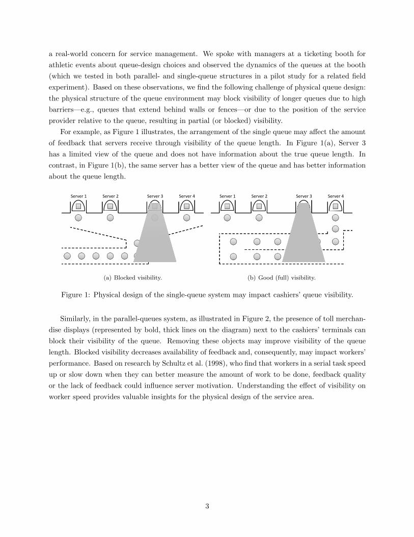
For example, as Figure 1 illustrates, the arrangement of the single queue may affect the amount
of feedback that servers receive through visibility of the queue length. In Figure 1(a), Server 3
has a limited view of the queue and does not have information about the true queue length. In
contrast, in Figure 1(b), the same server has a better view of the queue and has better information
about the queue length.
Server 1 Server 2 Server 3 Server 4
(a) Blocked visibility.
Server 1 Server 2 Server 3 Server 4
(b) Good (full) visibility.
Figure 1: Physical design of the single-queue system may impact cashiers’ queue visibility.
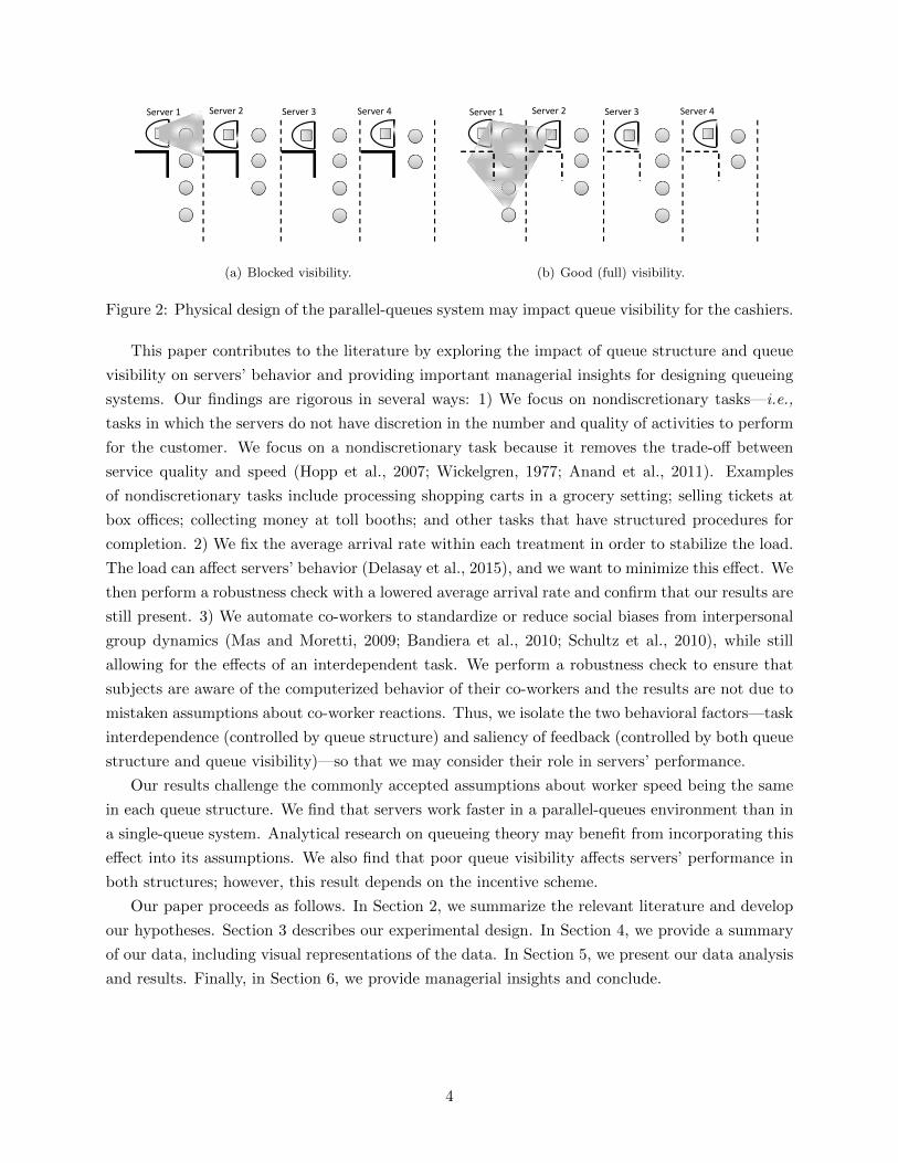
Similarly, in the parallel-queues system, as illustrated in Figure 2, the presence of toll merchan-
dise displays (represented by bold, thick lines on the diagram) next to the cashiers’ terminals can
block their visibility of the queue. Removing these objects may improve visibility of the queue
length. Blocked visibility decreases availability of feedback and, consequently, may impact workers’
performance. Based on research by Schultz et al. (1998), who find that workers in a serial task speed
up or slow down when they can better measure the amount of work to be done, feedback quality
or the lack of feedback could influence server motivation. Understanding the effect of visibility on
worker speed provides valuable insights for the physical design of the service area.
3
Server 1 Server 2 Server 3 Server 4
(a) Blocked visibility.
Server 1 Server 2 Server 3 Server 4
(b) Good (full) visibility.
Figure 2: Physical design of the parallel-queues system may impact queue visibility for the cashiers.
This paper contributes to the literature by exploring the impact of queue structure and queue
visibility on servers’ behavior and providing important managerial insights for designing queueing
systems. Our findings are rigorous in several ways: 1) We focus on nondiscretionary tasks—i.e.,
tasks in which the servers do not have discretion in the number and quality of activities to perform
for the customer. We focus on a nondiscretionary task because it removes the trade-off between
service quality and speed (Hopp et al., 2007; Wickelgren, 1977; Anand et al., 2011). Examples
of nondiscretionary tasks include processing shopping carts in a grocery setting; selling tickets at
box offices; collecting money at toll booths; and other tasks that have structured procedures for
completion. 2) We fix the average arrival rate within each treatment in order to stabilize the load.
The load can affect servers’ behavior (Delasay et al., 2015), and we want to minimize this effect. We
then perform a robustness check with a lowered average arrival rate and confirm that our results are
still present. 3) We automate co-workers to standardize or reduce social biases from interpersonal
group dynamics (Mas and Moretti, 2009; Bandiera et al., 2010; Schultz et al., 2010), while still
allowing for the effects of an interdependent task. We perform a robustness check to ensure that
subjects are aware of the computerized behavior of their co-workers and the results are not due to
mistaken assumptions about co-worker reactions. Thus, we isolate the two behavioral factors—task
interdependence (controlled by queue structure) and saliency of feedback (controlled by both queue
structure and queue visibility)—so that we may consider their role in servers’ performance.
Our results challenge the commonly accepted assumptions about worker speed being the same
in each queue structure. We find that servers work faster in a parallel-queues environment than in
a single-queue system. Analytical research on queueing theory may benefit from incorporating this
effect into its assumptions. We also find that poor queue visibility affects servers’ performance in
both structures; however, this result depends on the incentive scheme.
Our paper proceeds as follows. In Section 2, we summarize the relevant literature and develop
our hypotheses. Section 3 describes our experimental design. In Section 4, we provide a summary
of our data, including visual representations of the data. In Section 5, we present our data analysis
and results. Finally, in Section 6, we provide managerial insights and conclude.
4
2 Literature Review and Hypotheses Development
The research questions posed in Bendoly et al. (2010) indicate a need to consider both task in-
terdependence and feedback. In this section, we provide an overview of the literature underlying
these factors and form the two main hypotheses of our paper. Additionally, we consider studies
that focus on effort in groups and/or queueing settings to provide additional foundation for the
experimental assumptions made in our study.
Working in groups changes the perception of output relative to effort. Williams et al. (1981)
attribute the reduction in workers’ individual effort in a group setting—as opposed to an individual
setting–to social loafing, and Karau and Williams (1993) summarize several theories that have
been proposed to explain the phenomenon. One of these theories, dispensability of effort, is closely
related to our study: it is driven by task interdependence, which is present in the single-queue
environment. In such an environment, the servers work collectively to clear the customer queue,
and, hence, individual effort is dispensable, which is consistent with the hypotheses of Bendoly
et al. (2010). Pearce and Gregersen (1991) explain that workers feel less responsibility for the task
due to interdependence, and Kidwell and Bennett (1993) claim that “[g]reater task interdependence
will be positively related to propensity to withhold effort.” (Hypothesis 8, page 446)
Note that this interdependence is present regardless of the visibility of the other servers; and it
may be present regardless of whether the workload is shared with a human server, a machine, or
a virtual co-worker because it is about the shared effort across the pool of co-workers, not social
pressure. In a parallel-queues system, because servers have their own queues, their performance has
a direct impact on the speed at which their line moves. Moreover, the servers face every customer
who joins their queue. If customers join the shortest queue, each server also influences the total
workload of other servers, but servers are likely to view their queue as their responsibility. In
contrast, in the single-queue environment, servers work together to process one common queue,
and, thus, the impact of each individual’s effort is less apparent. In both approaches, the work is
collective, in that the workers jointly manage the final goal of processing all incoming customers.
However, the interdependence makes the collective nature more clear in the single-queue than in the
parallel-queues system (Bendoly et al., 2010). Because co-workers are known to be pre-programmed
computers, we emphasize that this study is about the task interdependence mechanism, not about
the more general concepts of social loafing. We can now state our first hypothesis:
Hypothesis 1 (Impact of queue structure) Servers work faster in the queueing environment
in which customers are aligned into multiple parallel queues instead of a single pooled queue.
Separate from the various concepts of social loafing, control theory, discussed in the behavioral
literature, tells us that workers use feedback about their actual performance relative to a goal
to self-regulate behavior (Donovan, 2001; Bendoly et al., 2010). Schultz et al. (2003) and Powell
and Schultz (2004) find that workers adjust their speeds more when feedback about performance
becomes more salient, such as when low-inventory buffers allow observation of fast and slow points
in a production line. Goal setting in conjunction with feedback leads to performance improvements
5
(Erez, 1977), but feedback alone can also lead to improvements (Latham and Locke, 1991). This
feedback can take the form of monitoring the changes to work-in-process, where the ability to view
changes in inventory levels changes worker behavior (Schultz et al., 2003; Powell and Schultz, 2004).
That is, the visibility of the workload affects worker effort, leading to our second hypothesis:
Hypothesis 2 (Impact of queue visibility) Servers work more slowly in a queueing environ-
ment with blocked (poor) queue visibility than in an environment with full (good) visibility.
Note that both behavioral mechanisms, task interdependence and feedback, suggest a slower
server performance in a single-queue structure: relative to parallel queues, the single-queue structure
has higher task interdependence and lower feedback, both leading to a reduction in effort. Hence,
observing a decrease in service rate in the single-queue structure does not indicate which behavioral
mechanism is causing the decreased effort. Manipulating visibility of the system allows us to
disentangle the impact: under blocked visibility, there is no feedback in either single- or parallel-
queue structures. Thus, observing a slowdown in service rate in a single-queue system under
blocked visibility indicates that the task interdependence mechanism is causing the slowdown.
If the slowdown is observed only under good visibility, the slowdown is caused by the feedback
mechanism.
Clearly, effort exerted by servers also depends on the provided rewards. Based on transaction
cost economics (Williamson, 1975; Jones, 1984), we know that “employees have strong incentives
to shirk and no incentive to improve performance unless task conditions allow them to demonstrate
discrete performance contributions and to obtain related rewards” (Kidwell and Bennett, 1993,
p. 445). Gilbert and Weng (1998) explore the impact of rewards in a related setting with pooled
queue structures. In an analytical study on compensation and workload allocation, they find
reduced benefit from pooling when two competing symmetric employees set a costly effort level,
are compensated per customer, and compete with other servers for tasks. In our behavioral work,
we also explore the effect of compensation on effort by including an incentive structure factor with
two payment schemes: flat payment and pay-for-performance.
By studying dispensability of effort driven by task interdependence and saliency of feedback,
we focus on structural drivers of effort reduction that occur without social interaction. However,
there are other drivers of effort reduction in group settings that arise from social and strategic
interactions between human co-workers. Such interactions have been addressed by, for example,
Mas and Moretti (2009), who find that a worker’s productivity improves when a highly productive
employee is introduced into a group of parallel-queues workers. This occurs when there is a previous
relationship, and the workers know that the faster employee can see them. Similar results show
that workers are affected by peer relationships within their teams, such as friendships and enmities
(Bandiera et al., 2010). Several studies show that individuals will converge to the average—such
that fast workers slow down and slow workers speed up—a pattern known as equity theory (Schultz
et al., 1998, 1999, 2010). Most of these studies are done in conjunctive (serial) tasks in which one
subject’s output depends on another upstream teammate’s output. Schultz et al. (2010) present
6
evidence supporting equity theory in an additive task with a common buffer, which is similar
to a single-queue setting. Additional interpersonal issues are tied to the physical structure and
design of the queue and affect our subjects: dehumanization of teammates via lack of physical
presence (Alnuaimi et al., 2010), framing of bonuses (Hossain and List, 2012), etc. In our study, all
subjects had the same degree of physical separation from their computerized co-workers that had
equal processing speeds on average and all payments occurred at the end to control for possible
interpersonal issues and focus on queue structure and queue visibility rather than on peer effects.
A number of previous studies show that servers can adjust their service speed in response to the
environment, rather than working at a stationary average speed (as early analytical work assumed).
This includes reacting to the type of task, the work load, and the pay structure. Analytical work
finds that the value of queue pooling is reduced when servers have discretion over the number or
quality of tasks to perform for a given customer (i.e., discretionary tasks) (Cachon and Zhang,
2007; Jouini et al., 2008; Debo et al., 2008; Hopp et al., 2007, 2009). Behavioral studies show that
when tasks are discretionary, workers will speed up or slow down to keep up or to appear busy
with a higher load, as necessary, particularly to meet external incentives (Tan and Netessine, 2014;
Oliva and Sterman, 2001; Hasija et al., 2010). While discretion is an interesting factor, our study
was concerned primarily with the impact of the queue design on server performance. Therefore,
to minimize the effect of discretion, we focus on nondiscretionary tasks, which are very common
in practice (checking out customers in a grocery setting, selling tickets, processing registration
information, etc). Additionally, Joustra et al. (2010) show analytically that pooling is ineffective
when merging distinct customer types, so all of our customers have comparable carts. Finally,
in studying environmental factors in queueing systems, previous studies find that load can affect
service rates (see Delasay et al. 2015 for a detailed summary). We set the queue parameters so
that all subjects in a treatment face similar average arrival rates, and we test our study under both
high and low load.
Our research is most closely related to the empirical work of Song et al. (2015) and Wang and
Zhou (2015). Song et al. (2015) examine the impact of queue pooling in a healthcare setting. They
find that patient length-of-stay is ten-percent shorter when physicians are assigned patients under a
parallel (dedicated-queue) system, compared to when the physicians work together under a pooled
(single-queue) system. This indicates that workers slow down when working with a single queue,
as opposed to parallel-queues. The healthcare environment, however, has highly variable customer
care requirements that are further compounded by the nature of discretionary task completion,
meaning that service providers have discretion over the number of tasks to perform for a given
patient. Wang and Zhou (2015) study parallel queues and single queues running simultaneously in
a grocery store and find empirical evidence that workers slow down in pooled queues. These results
support our first hypothesis in complex empirical settings.
Our study contributes to this literature by testing our hypotheses through a controlled labo-
ratory experiment, which allows us not only to demonstrate the slowdown effect in a single-queue
structure, but also to separate the behavioral mechanisms behind the servers’ slowdown: task
7
interdependence and feedback availability. Identifying which mechanism is causing the servers’
slowdown guides managers in selecting remedial actions.
3 Experimental Design
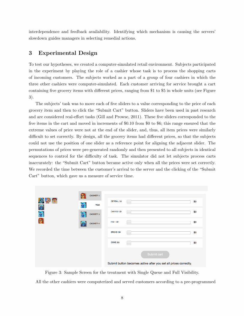
To test our hypotheses, we created a computer-simulated retail environment. Subjects participated
in the experiment by playing the role of a cashier whose task is to process the shopping carts
of incoming customers. The subjects worked as a part of a group of four cashiers in which the
three other cashiers were computer-simulated. Each customer arriving for service brought a cart
containing five grocery items with different prices, ranging from $1 to $5 in whole units (see Figure
3).
The subjects’ task was to move each of five sliders to a value corresponding to the price of each
grocery item and then to click the “Submit Cart” button. Sliders have been used in past research
and are considered real-effort tasks (Gill and Prowse, 2011). These five sliders corresponded to the
five items in the cart and moved in increments of $0.10 from $0 to $6; this range ensured that the
extreme values of price were not at the end of the slider, and, thus, all item prices were similarly
difficult to set correctly. By design, all the grocery items had different prices, so that the subjects
could not use the position of one slider as a reference point for aligning the adjacent slider. The
permutations of prices were pre-generated randomly and then presented to all subjects in identical
sequences to control for the difficulty of task. The simulator did not let subjects process carts
inaccurately: the “Submit Cart” button became active only when all the prices were set correctly.
We recorded the time between the customer’s arrival to the server and the clicking of the “Submit
Cart” button, which gave us a measure of service time.
Figure 3: Sample Screen for the treatment with Single Queue and Full Visibility.
All the other cashiers were computerized and served customers according to a pre-programmed
8
process. Their service time for each customer was a random time set to ten seconds plus an expo-
nential random variable with a mean of ten seconds. We selected this distribution after examining
data from our pilot studies, in which we measured the subjects’ service time (the plot of service time
distribution from the pilot data is presented in Figure 9 in the Appendix, Section 7.3). Computer-
simulated customers arrived for service according to a Poisson process with a mean inter-arrival
time of 5.5 seconds. In the single-queue treatment, arriving customers joined the single queue;
in the parallel-queues treatment, arriving customers observed the system and joined the shortest
queue, with ties broken randomly. Customer jockeying is an important attribute of many real-world
queues; however, because we did not have a well-developed model for customer jockeying behavior
and because our main focus was on the server behavior, we omitted this aspect from the current
study. Note that while customers already in the system did not jockey between the queues, the
arriving customers always joined the shortest queue; this led to a distribution of customers that
was fairly balanced among the queues during the experiment. Hence, we assumed that adding
jockeying would not make a large change to the balance of load among the queues.1 The simulator
was initialized with customers already present in the queue to make sure that the subjects could
immediately start working and that the system would achieve steady state relatively quickly. In
the single-queue setting: one customer at each server and eight customers in the shared queue (for
a total of 12 customers: 8 waiting and 4 in service); in the parallel-queues setting: one customer
at each server and three customers in each queue (for a total of 16 customers: 12 waiting and 4
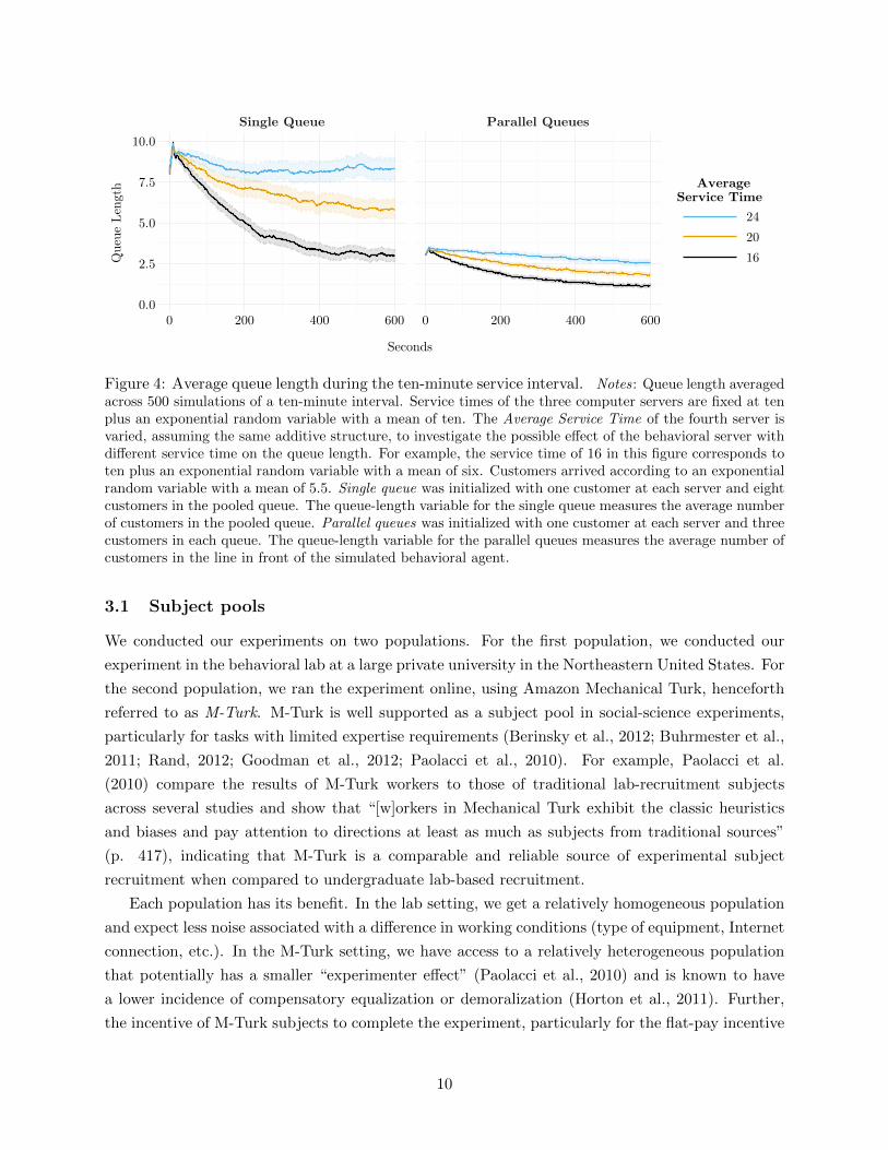
in service). To calibrate the parameters (arrival rate, service time of computerized servers, and
initial queue length parameters), we simulated our experiment with different values and assessed
the evolution of average queue length and average utilization in the system during the ten-minute
experimental round. We then chose values for which each system could achieve the steady state
within the allocated time for a variety of potential participants’ service times (as evidenced by the
plots in Figure 4) and for which the two queue structures had similar utilization (as evidenced by
the plots of the average server’s utilization in Figure 12 in the Appendix).
1We demonstrate this in Figure 13 in the Appendix, which shows the distribution of queue length assumingjockeying next to the distribution of queue length assuming that customers join the shortest queue, as implementedin our study.
9
Single Queue Parallel Queues
0.0
2.5
5.0
7.5
10.0
0 200 400 600 0 200 400 600
Seconds
Que
ue L
engt
h Average Service Time
24
20
16
Figure 4: Average queue length during the ten-minute service interval. Notes: Queue length averagedacross 500 simulations of a ten-minute interval. Service times of the three computer servers are fixed at tenplus an exponential random variable with a mean of ten. The Average Service Time of the fourth server isvaried, assuming the same additive structure, to investigate the possible effect of the behavioral server withdifferent service time on the queue length. For example, the service time of 16 in this figure corresponds toten plus an exponential random variable with a mean of six. Customers arrived according to an exponentialrandom variable with a mean of 5.5. Single queue was initialized with one customer at each server and eightcustomers in the pooled queue. The queue-length variable for the single queue measures the average numberof customers in the pooled queue. Parallel queues was initialized with one customer at each server and threecustomers in each queue. The queue-length variable for the parallel queues measures the average number ofcustomers in the line in front of the simulated behavioral agent.
3.1 Subject pools
We conducted our experiments on two populations. For the first population, we conducted our
experiment in the behavioral lab at a large private university in the Northeastern United States. For
the second population, we ran the experiment online, using Amazon Mechanical Turk, henceforth
referred to as M-Turk. M-Turk is well supported as a subject pool in social-science experiments,
particularly for tasks with limited expertise requirements (Berinsky et al., 2012; Buhrmester et al.,
2011; Rand, 2012; Goodman et al., 2012; Paolacci et al., 2010). For example, Paolacci et al.
(2010) compare the results of M-Turk workers to those of traditional lab-recruitment subjects
across several studies and show that “[w]orkers in Mechanical Turk exhibit the classic heuristics
and biases and pay attention to directions at least as much as subjects from traditional sources”
(p. 417), indicating that M-Turk is a comparable and reliable source of experimental subject
recruitment when compared to undergraduate lab-based recruitment.
Each population has its benefit. In the lab setting, we get a relatively homogeneous population
and expect less noise associated with a difference in working conditions (type of equipment, Internet
connection, etc.). In the M-Turk setting, we have access to a relatively heterogeneous population
that potentially has a smaller “experimenter effect” (Paolacci et al., 2010) and is known to have
a lower incidence of compensatory equalization or demoralization (Horton et al., 2011). Further,
the incentive of M-Turk subjects to complete the experiment, particularly for the flat-pay incentive
10
scheme, may be closer to the real-world workers’ incentive in many practical settings. Specifically,
subjects may be worried about their reputation and their ability to get future jobs because they
may be affected by the low rankings received on M-Turk from the experiment requesters.
3.2 Experimental flow
The experiment proceeded in the same manner for both populations. First, all subjects were
exposed to a series of instruction screens that provided a description of the experimental environ-
ment and task, as well as a visual example of the experiment (see Section 7.1 in the Appendix
for a complete set of instructions). Each subject then completed a two-minute training session
to become familiar with the interface and sliders. After this training, the subjects completed a
ten-minute round of the experiment. At the end of the experiment, the subjects completed an exit
survey from which we collected demographic information, information regarding subjects’ manage-
rial experience, and, for the M-Turk population, information on the type of input device (external
mouse, touchpad, touchscreen) the subjects used to move the sliders. Finally, the subjects received
payment. Each subject was allowed to participate in the experiment only once.
3.3 Incentive settings
To capture different practical settings, we ran the experiments under two different incentive settings:
Flat Pay, by which all subjects received a fixed payment for completing the experiment regardless
of their performance (e.g., student employees at a university athletics ticketing booth who receive
a fixed hourly wage); and Per Cart, by which subjects received a small fixed pay and a bonus per
each completed cart (e.g., cashiers at a retail store who have incentives based on items scanned per
minute). We explained the Per Cart payment scheme to the participants in the following way:
You will earn $0.25 ($0.04 on M-Turk) for each customer that you successfully submit.
Thus, if you complete ten customers, you will earn $2.50 ($0.40) in addition to the
$2.00 ($0.50) participation payment.
Then, we checked that the subjects understood the payment scheme by having them compute the
payoff for a sample scenario. In the case of a wrong answer, we repeated the instructions and had
them compute the payoff again until they answered correctly.
The subjects in the M-Turk population were paid $1.25 for participation in the 30-minute
experiment regardless of their performance in the Flat Pay setting, and a fixed fee of $0.50 in
the Per Cart setting plus $0.04 per each completed cart, with an average total payoff of $1.47.2
The subjects in the lab population were paid $5.00 for participation in the 30-minute experiment
regardless of their performance in the Flat Pay setting, and a fixed fee of $2.00 in the Per Cart
setting plus $0.25 per each completed cart, with an average payoff of $9.65.
2This was a relatively high pay rate for M-Turk subjects (typical rates are $0.10–0.50 per study with a typicalrate of $1.40 per hour (Horton and Chilton, 2010)).
11
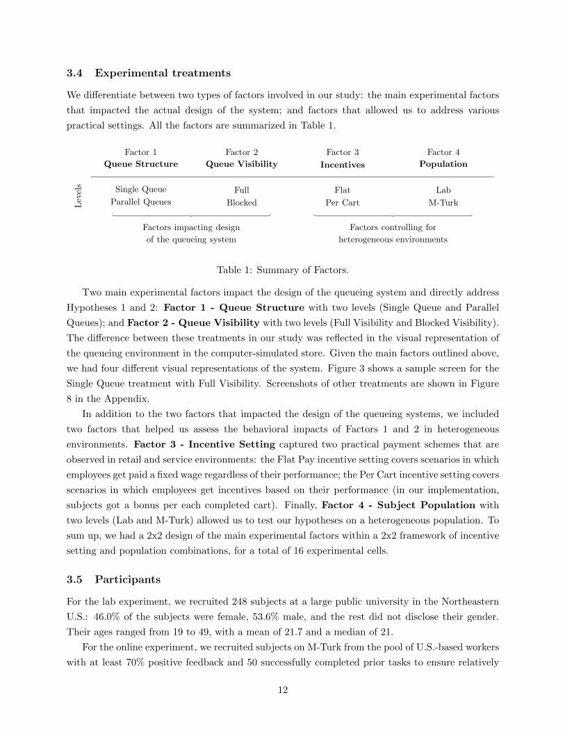
3.4 Experimental treatments
We differentiate between two types of factors involved in our study: the main experimental factors
that impacted the actual design of the system; and factors that allowed us to address various
practical settings. All the factors are summarized in Table 1.
Levels
Factor 1
Queue Structure
Single Queue
Parallel Queues
Factor 2
Queue Visibility
Full
Blocked
Factor 3
Incentives
Flat
Per Cart
Factor 4
Population
Lab
M-Turk
Factors impacting design
of the queueing system
Factors controlling for
heterogeneous environments
Table 1: Summary of Factors.
Two main experimental factors impact the design of the queueing system and directly address
Hypotheses 1 and 2: Factor 1 - Queue Structure with two levels (Single Queue and Parallel
Queues); and Factor 2 - Queue Visibility with two levels (Full Visibility and Blocked Visibility).
The difference between these treatments in our study was reflected in the visual representation of
the queueing environment in the computer-simulated store. Given the main factors outlined above,
we had four different visual representations of the system. Figure 3 shows a sample screen for the
Single Queue treatment with Full Visibility. Screenshots of other treatments are shown in Figure
8 in the Appendix.
In addition to the two factors that impacted the design of the queueing systems, we included
two factors that helped us assess the behavioral impacts of Factors 1 and 2 in heterogeneous
environments. Factor 3 - Incentive Setting captured two practical payment schemes that are
observed in retail and service environments: the Flat Pay incentive setting covers scenarios in which
employees get paid a fixed wage regardless of their performance; the Per Cart incentive setting covers
scenarios in which employees get incentives based on their performance (in our implementation,
subjects got a bonus per each completed cart). Finally, Factor 4 - Subject Population with
two levels (Lab and M-Turk) allowed us to test our hypotheses on a heterogeneous population. To
sum up, we had a 2x2 design of the main experimental factors within a 2x2 framework of incentive
setting and population combinations, for a total of 16 experimental cells.
3.5 Participants
For the lab experiment, we recruited 248 subjects at a large public university in the Northeastern
U.S.: 46.0% of the subjects were female, 53.6% male, and the rest did not disclose their gender.
Their ages ranged from 19 to 49, with a mean of 21.7 and a median of 21.
For the online experiment, we recruited subjects on M-Turk from the pool of U.S.-based workers
with at least 70% positive feedback and 50 successfully completed prior tasks to ensure relatively
12
experienced computer users. Of the 481 unique subjects who completed the experiments on M-
Turk, 54.3% were female, 44.4% male, and the rest did not disclose their gender. Their ages ranged
from 19 to 51, with a mean of 34.1 and a median of 33.
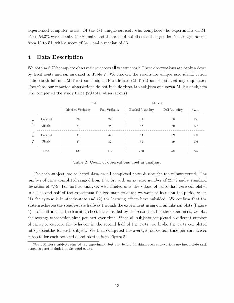
4 Data Description
We obtained 729 complete observations across all treatments.3 These observations are broken down
by treatments and summarized in Table 2. We checked the results for unique user identification
codes (both lab and M-Turk) and unique IP addresses (M-Turk) and eliminated any duplicates.
Therefore, our reported observations do not include three lab subjects and seven M-Turk subjects
who completed the study twice (20 total observations).
Lab M-Turk
Blocked Visibility Full Visibility Blocked Visibility Full Visibility
Parallel
Single
Parallel
Single
Total
Total
Flat
Per
Cart
129 119 250 231
168
177
191
193
729
28
27
27
28
60
62
53
60
37
37
32
32
63
65
59
59
Table 2: Count of observations used in analysis.
For each subject, we collected data on all completed carts during the ten-minute round. The
number of carts completed ranged from 1 to 67, with an average number of 29.72 and a standard
deviation of 7.79. For further analysis, we included only the subset of carts that were completed
in the second half of the experiment for two main reasons: we want to focus on the period when
(1) the system is in steady-state and (2) the learning effects have subsided. We confirm that the
system achieves the steady-state halfway through the experiment using our simulation plots (Figure
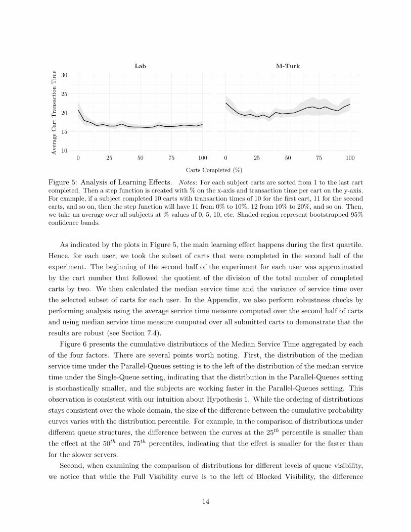
4). To confirm that the learning effect has subsided by the second half of the experiment, we plot
the average transaction time per cart over time. Since all subjects completed a different number
of carts, to capture the behavior in the second half of the carts, we broke the carts completed
into percentiles for each subject. We then computed the average transaction time per cart across
subjects for each percentile and plotted it in Figure 5.
3Some M-Turk subjects started the experiment, but quit before finishing; such observations are incomplete and,hence, are not included in the total count.
13
Lab M-Turk
10
15
20
25
30
0 25 50 75 100 0 25 50 75 100
Carts Completed (%)
Ave
rage
Car
t T
rans
action
Tim
e
Figure 5: Analysis of Learning Effects. Notes: For each subject carts are sorted from 1 to the last cartcompleted. Then a step function is created with % on the x-axis and transaction time per cart on the y-axis.For example, if a subject completed 10 carts with transaction times of 10 for the first cart, 11 for the secondcarts, and so on, then the step function will have 11 from 0% to 10%, 12 from 10% to 20%, and so on. Then,we take an average over all subjects at % values of 0, 5, 10, etc. Shaded region represent bootstrapped 95%confidence bands.
As indicated by the plots in Figure 5, the main learning effect happens during the first quartile.
Hence, for each user, we took the subset of carts that were completed in the second half of the
experiment. The beginning of the second half of the experiment for each user was approximated
by the cart number that followed the quotient of the division of the total number of completed
carts by two. We then calculated the median service time and the variance of service time over
the selected subset of carts for each user. In the Appendix, we also perform robustness checks by
performing analysis using the average service time measure computed over the second half of carts
and using median service time measure computed over all submitted carts to demonstrate that the
results are robust (see Section 7.4).
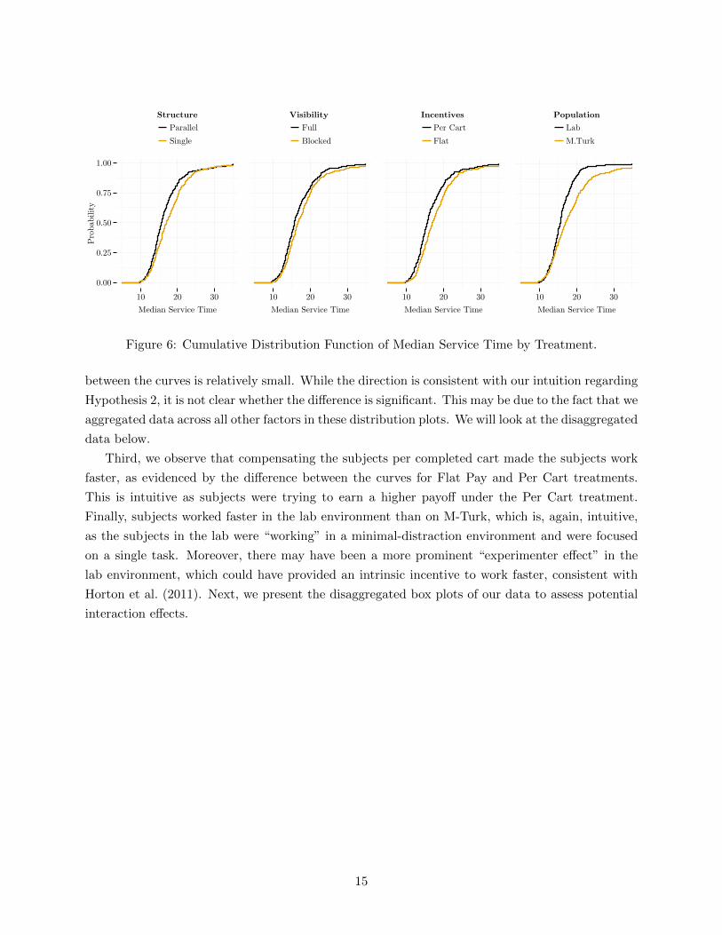
Figure 6 presents the cumulative distributions of the Median Service Time aggregated by each
of the four factors. There are several points worth noting. First, the distribution of the median
service time under the Parallel-Queues setting is to the left of the distribution of the median service
time under the Single-Queue setting, indicating that the distribution in the Parallel-Queues setting
is stochastically smaller, and the subjects are working faster in the Parallel-Queues setting. This
observation is consistent with our intuition about Hypothesis 1. While the ordering of distributions
stays consistent over the whole domain, the size of the difference between the cumulative probability
curves varies with the distribution percentile. For example, in the comparison of distributions under
different queue structures, the difference between the curves at the 25th percentile is smaller than
the effect at the 50th and 75th percentiles, indicating that the effect is smaller for the faster than
for the slower servers.
Second, when examining the comparison of distributions for different levels of queue visibility,
we notice that while the Full Visibility curve is to the left of Blocked Visibility, the difference
14
0.00
0.25
0.50
0.75
1.00
10 20 30
Median Service Time
Pro
babi
lity
StructureParallel
Single
10 20 30
Median Service Time
VisibilityFull
Blocked
10 20 30
Median Service Time
IncentivesPer Cart
Flat
10 20 30
Median Service Time
PopulationLab
M.Turk
Figure 6: Cumulative Distribution Function of Median Service Time by Treatment.
between the curves is relatively small. While the direction is consistent with our intuition regarding
Hypothesis 2, it is not clear whether the difference is significant. This may be due to the fact that we
aggregated data across all other factors in these distribution plots. We will look at the disaggregated
data below.
Third, we observe that compensating the subjects per completed cart made the subjects work
faster, as evidenced by the difference between the curves for Flat Pay and Per Cart treatments.
This is intuitive as subjects were trying to earn a higher payoff under the Per Cart treatment.
Finally, subjects worked faster in the lab environment than on M-Turk, which is, again, intuitive,
as the subjects in the lab were “working” in a minimal-distraction environment and were focused
on a single task. Moreover, there may have been a more prominent “experimenter effect” in the
lab environment, which could have provided an intrinsic incentive to work faster, consistent with
Horton et al. (2011). Next, we present the disaggregated box plots of our data to assess potential
interaction effects.
15
Lab M-Turk
10
20
30
10
20
30
Flat
Per C
art
Blocked Visibility Full Visibility Blocked Visibility Full Visibility
Med
ian
Serv
ice
Tim
e
Structure: Single Parallel
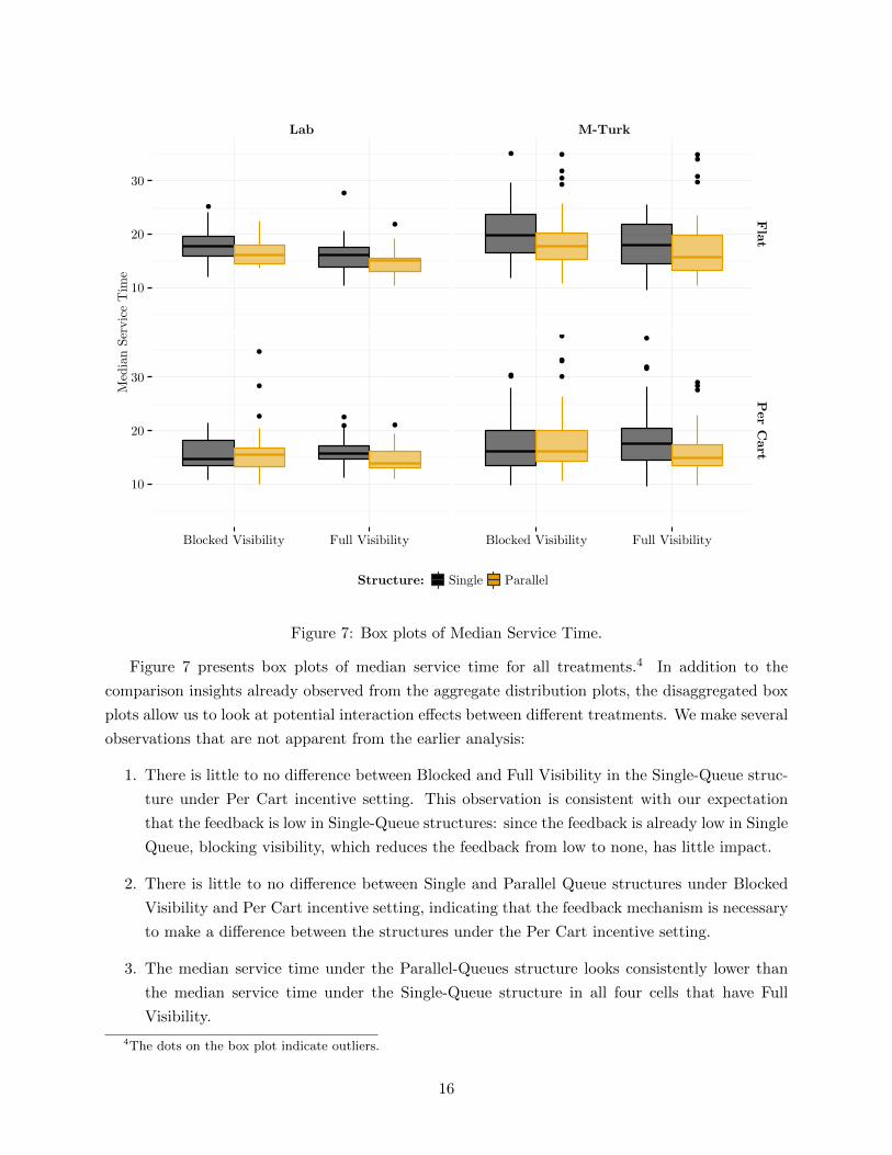
Figure 7: Box plots of Median Service Time.
Figure 7 presents box plots of median service time for all treatments.4 In addition to the
comparison insights already observed from the aggregate distribution plots, the disaggregated box
plots allow us to look at potential interaction effects between different treatments. We make several
observations that are not apparent from the earlier analysis:
1. There is little to no difference between Blocked and Full Visibility in the Single-Queue struc-
ture under Per Cart incentive setting. This observation is consistent with our expectation
that the feedback is low in Single-Queue structures: since the feedback is already low in Single
Queue, blocking visibility, which reduces the feedback from low to none, has little impact.
2. There is little to no difference between Single and Parallel Queue structures under Blocked
Visibility and Per Cart incentive setting, indicating that the feedback mechanism is necessary
to make a difference between the structures under the Per Cart incentive setting.
3. The median service time under the Parallel-Queues structure looks consistently lower than
the median service time under the Single-Queue structure in all four cells that have Full
Visibility.
4The dots on the box plot indicate outliers.
16
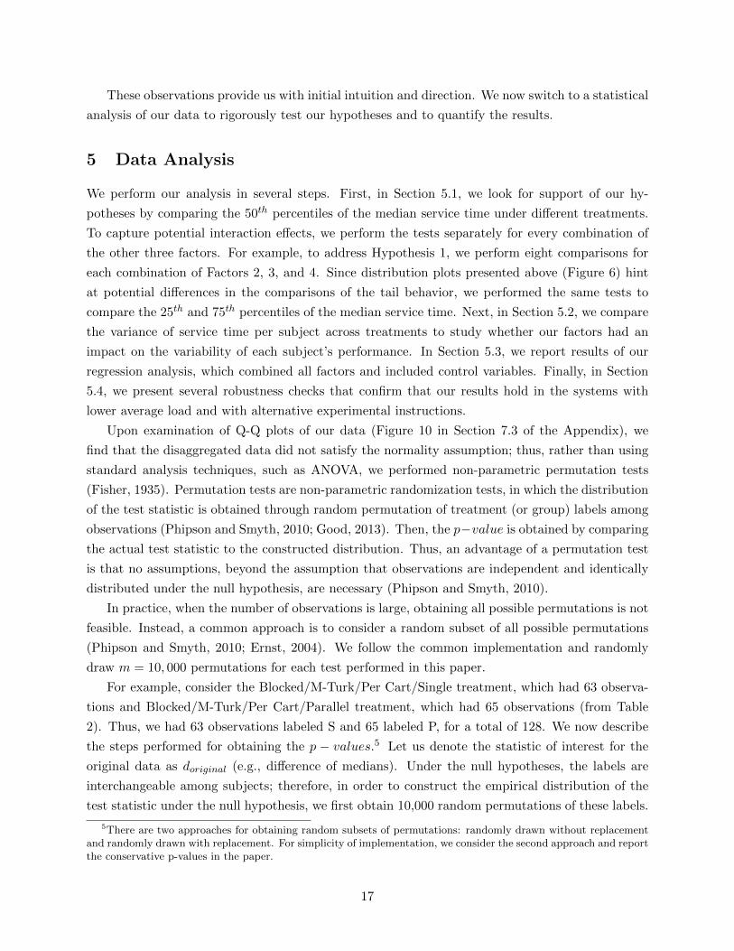
These observations provide us with initial intuition and direction. We now switch to a statistical
analysis of our data to rigorously test our hypotheses and to quantify the results.
5 Data Analysis
We perform our analysis in several steps. First, in Section 5.1, we look for support of our hy-
potheses by comparing the 50th percentiles of the median service time under different treatments.
To capture potential interaction effects, we perform the tests separately for every combination of
the other three factors. For example, to address Hypothesis 1, we perform eight comparisons for
each combination of Factors 2, 3, and 4. Since distribution plots presented above (Figure 6) hint
at potential differences in the comparisons of the tail behavior, we performed the same tests to
compare the 25th and 75th percentiles of the median service time. Next, in Section 5.2, we compare
the variance of service time per subject across treatments to study whether our factors had an
impact on the variability of each subject’s performance. In Section 5.3, we report results of our
regression analysis, which combined all factors and included control variables. Finally, in Section
5.4, we present several robustness checks that confirm that our results hold in the systems with
lower average load and with alternative experimental instructions.
Upon examination of Q-Q plots of our data (Figure 10 in Section 7.3 of the Appendix), we
find that the disaggregated data did not satisfy the normality assumption; thus, rather than using
standard analysis techniques, such as ANOVA, we performed non-parametric permutation tests
(Fisher, 1935). Permutation tests are non-parametric randomization tests, in which the distribution
of the test statistic is obtained through random permutation of treatment (or group) labels among
observations (Phipson and Smyth, 2010; Good, 2013). Then, the p−value is obtained by comparing
the actual test statistic to the constructed distribution. Thus, an advantage of a permutation test
is that no assumptions, beyond the assumption that observations are independent and identically
distributed under the null hypothesis, are necessary (Phipson and Smyth, 2010).
In practice, when the number of observations is large, obtaining all possible permutations is not
feasible. Instead, a common approach is to consider a random subset of all possible permutations
(Phipson and Smyth, 2010; Ernst, 2004). We follow the common implementation and randomly
draw m = 10, 000 permutations for each test performed in this paper.
For example, consider the Blocked/M-Turk/Per Cart/Single treatment, which had 63 observa-
tions and Blocked/M-Turk/Per Cart/Parallel treatment, which had 65 observations (from Table
2). Thus, we had 63 observations labeled S and 65 labeled P, for a total of 128. We now describe
the steps performed for obtaining the p − values.5 Let us denote the statistic of interest for the
original data as doriginal (e.g., difference of medians). Under the null hypotheses, the labels are
interchangeable among subjects; therefore, in order to construct the empirical distribution of the
test statistic under the null hypothesis, we first obtain 10,000 random permutations of these labels.
5There are two approaches for obtaining random subsets of permutations: randomly drawn without replacementand randomly drawn with replacement. For simplicity of implementation, we consider the second approach and reportthe conservative p-values in the paper.
17
Next, for each permutation, we obtain the statistic of interest, dpermut and find a number of per-
mutations, b, for which the statistic of interest exceeds or is equal to doriginal. Finally, we obtain
the p− value as p = b+1m+1 (Phipson and Smyth, 2010; Ernst, 2004).
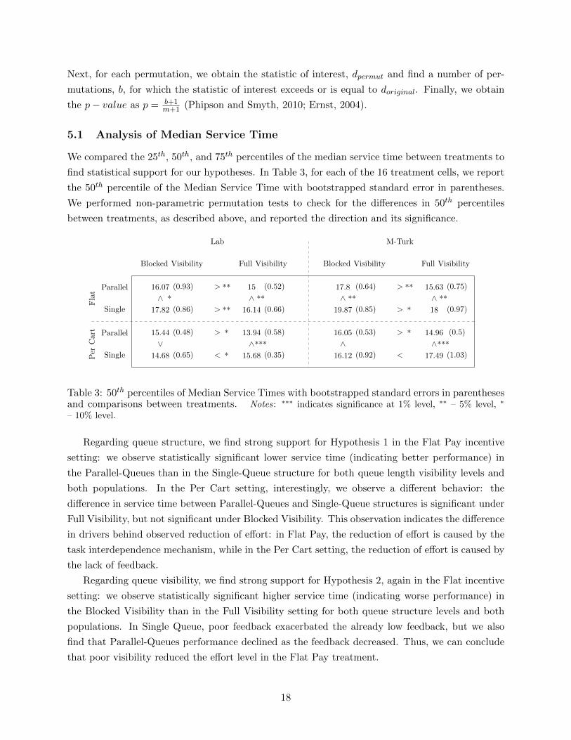
5.1 Analysis of Median Service Time
We compared the 25th, 50th, and 75th percentiles of the median service time between treatments to
find statistical support for our hypotheses. In Table 3, for each of the 16 treatment cells, we report
the 50th percentile of the Median Service Time with bootstrapped standard error in parentheses.
We performed non-parametric permutation tests to check for the differences in 50th percentiles
between treatments, as described above, and reported the direction and its significance.
Lab M-Turk
Flat
Per
Cart
Blocked Visibility Full Visibility Blocked Visibility Full Visibility
Parallel
Single
Parallel
Single
Lab M-Turk
Flat
Per
Cart
Blocked Visibility Full Visibility Blocked Visibility Full Visibility
Parallel
Single
Parallel
Single
Lab M-Turk
Flat
Per
Cart
Blocked Visibility Full Visibility Blocked Visibility Full Visibility
Parallel
Single
Parallel
Single
Lab M-Turk
Flat
Per
Cart
Blocked Visibility Full Visibility Blocked Visibility Full Visibility
Parallel
Single
Parallel
Single
Lab M-Turk
Flat
Per
Cart
Blocked Visibility Full Visibility Blocked Visibility Full Visibility
Parallel
Single
Parallel
Single
16.54 (0.46)
2.45 (0.3)
14.35 (0.37)
16.07 (0.93)
17.92 (0.66)
>***
>
>***
> **
> **
> *
>> **
> *
> *
14.62 (0.49)
2.42 (0.43)
12.91 (0.71)
15 (0.52)
15.54 (0.42)
> **
>>
> **
> **
18.99 (0.73)
5.95 (1)
15.19 (0.69)
17.8 (0.64)
20.22 (0.84)
>
<
> **
> **
>
>***
> **
> *
> **
> **
17.72 (0.9)
6.61 (1.16)
13.23 (0.48)
15.63 (0.75)
19.79 (1.2)
>< **
> *
> **
>
17.59 (0.56)
3.03 (0.47)
15.8 (0.52)
17.82 (0.86)
19.53 (0.66)
> *
<
> *
> **
> *
16.26 (0.66)
3.6 (0.65)
13.76 (0.92)
16.14 (0.66)
17.5 (1.07)
24.27 (2.15)
16.95 (4.21)
16.49 (0.64)
19.87 (0.85)
23.72 (1.59)
>***
>***
> **
> *
> **
18.01 (0.56)
4.2 (0.26)
14.35 (0.84)
18 (0.97)
21.79 (0.8)
15.95 (0.76)
4.76 (1.08)
13.18 (0.82)
15.44 (0.48)
16.79 (0.8)
>
> *
>
> *
>
<<
><
>
14.77 (0.44)
2.5 (0.3)
13.11 (0.44)
13.94 (0.58)
16.02 (0.83)
> **
>>***
>***
>
17.49 (0.68)
5.51 (0.79)
14.24 (0.54)
16.05 (0.53)
20.02 (1.23)
>
<
>
> *
> **
<>
<>
>
16.52 (0.88)
6.85 (2.04)
13.37 (0.42)
14.96 (0.5)
17.37 (0.82)
> **
>> **
>***
> **
15.56 (0.45)
2.82 (0.26)
13.5 (0.35)
14.68 (0.65)
18.2 (0.98)
<
>
< **
< *
>
16.1 (0.46)
2.59 (0.35)
14.69 (0.53)
15.68 (0.35)
17.19 (0.81)
17.47 (0.7)
5.69 (0.82)
13.5 (0.5)
16.12 (0.92)
20.09 (0.93)
< *
<
< *
<
<
19.41 (1.32)
10.16 (3.56)
14.49 (0.46)
17.49 (1.03)
20.42 (1.14)
Table 3: 50th percentiles of Median Service Times with bootstrapped standard errors in parenthesesand comparisons between treatments. Notes: ∗∗∗ indicates significance at 1% level, ∗∗ – 5% level, ∗
– 10% level.
Regarding queue structure, we find strong support for Hypothesis 1 in the Flat Pay incentive
setting: we observe statistically significant lower service time (indicating better performance) in
the Parallel-Queues than in the Single-Queue structure for both queue length visibility levels and
both populations. In the Per Cart setting, interestingly, we observe a different behavior: the
difference in service time between Parallel-Queues and Single-Queue structures is significant under
Full Visibility, but not significant under Blocked Visibility. This observation indicates the difference
in drivers behind observed reduction of effort: in Flat Pay, the reduction of effort is caused by the
task interdependence mechanism, while in the Per Cart setting, the reduction of effort is caused by
the lack of feedback.
Regarding queue visibility, we find strong support for Hypothesis 2, again in the Flat incentive
setting: we observe statistically significant higher service time (indicating worse performance) in
the Blocked Visibility than in the Full Visibility setting for both queue structure levels and both
populations. In Single Queue, poor feedback exacerbated the already low feedback, but we also
find that Parallel-Queues performance declined as the feedback decreased. Thus, we can conclude
that poor visibility reduced the effort level in the Flat Pay treatment.
18
The impact of visibility manipulation in the Per Cart incentive setting with Single Queue
deserves special attention: we observe that, in the lab population, the effect of visibility went in
the opposite direction than predicted by Hypothesis 2. That is, Blocked Visibility sped up the
servers. This may be explained as follows: in the presence of per cart incentives, the subjects tried
to complete as many carts as possible. Without knowledge of how many potential customers were
present, the subjects tried to work as fast as possible to “steal” as many customers as possible from
the other servers, consistent with Gilbert and Weng (1998).
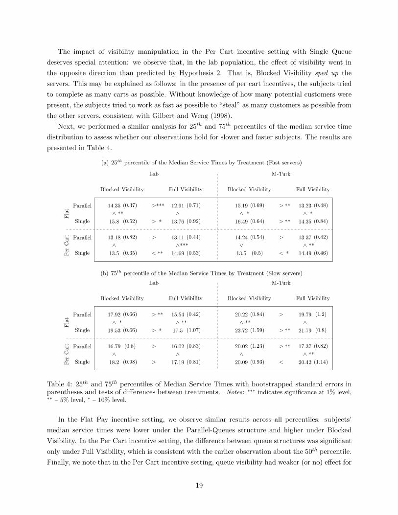
Next, we performed a similar analysis for 25th and 75th percentiles of the median service time
distribution to assess whether our observations hold for slower and faster subjects. The results are
presented in Table 4.
(a) 25th percentile of the Median Service Times by Treatment (Fast servers)
Lab M-Turk
Flat
Per
Cart
Blocked Visibility Full Visibility Blocked Visibility Full Visibility
Parallel
Single
Parallel
Single
Lab M-TurkFlat
Per
Cart
Blocked Visibility Full Visibility Blocked Visibility Full Visibility
Parallel
Single
Parallel
Single
Lab M-Turk
Flat
Per
Cart
Blocked Visibility Full Visibility Blocked Visibility Full Visibility
Parallel
Single
Parallel
Single
Lab M-Turk
Flat
Per
Cart
Blocked Visibility Full Visibility Blocked Visibility Full Visibility
Parallel
Single
Parallel
Single
Lab M-Turk
Flat
Per
Cart
Blocked Visibility Full Visibility Blocked Visibility Full Visibility
Parallel
Single
Parallel
Single
16.54 (0.46)
2.45 (0.3)
14.35 (0.37)
16.07 (0.93)
17.92 (0.66)
>***
>
>***
> **
> **
> *
>> **
> *
> *
14.62 (0.49)
2.42 (0.43)
12.91 (0.71)
15 (0.52)
15.54 (0.42)
> **
>>
> **
> **
18.99 (0.73)
5.95 (1)
15.19 (0.69)
17.8 (0.64)
20.22 (0.84)
>
<
> **
> **
>
>***
> **
> *
> **
> **
17.72 (0.9)
6.61 (1.16)
13.23 (0.48)
15.63 (0.75)
19.79 (1.2)
>< **
> *
> **
>
17.59 (0.56)
3.03 (0.47)
15.8 (0.52)
17.82 (0.86)
19.53 (0.66)
> *
<
> *
> **
> *
16.26 (0.66)
3.6 (0.65)
13.76 (0.92)
16.14 (0.66)
17.5 (1.07)
24.27 (2.15)
16.95 (4.21)
16.49 (0.64)
19.87 (0.85)
23.72 (1.59)
>***
>***
> **
> *
> **
18.01 (0.56)
4.2 (0.26)
14.35 (0.84)
18 (0.97)
21.79 (0.8)
15.95 (0.76)
4.76 (1.08)
13.18 (0.82)
15.44 (0.48)
16.79 (0.8)
>
> *
>
> *
>
<<
><
>
14.77 (0.44)
2.5 (0.3)
13.11 (0.44)
13.94 (0.58)
16.02 (0.83)
> **
>>***
>***
>
17.49 (0.68)
5.51 (0.79)
14.24 (0.54)
16.05 (0.53)
20.02 (1.23)
>
<
>
> *
> **
<>
<>
>
16.52 (0.88)
6.85 (2.04)
13.37 (0.42)
14.96 (0.5)
17.37 (0.82)
> **
>> **
>***
> **
15.56 (0.45)
2.82 (0.26)
13.5 (0.35)
14.68 (0.65)
18.2 (0.98)
<
>
< **
< *
>
16.1 (0.46)
2.59 (0.35)
14.69 (0.53)
15.68 (0.35)
17.19 (0.81)
17.47 (0.7)
5.69 (0.82)
13.5 (0.5)
16.12 (0.92)
20.09 (0.93)
< *
<
< *
<
<
19.41 (1.32)
10.16 (3.56)
14.49 (0.46)
17.49 (1.03)
20.42 (1.14)
(b) 75th percentile of the Median Service Times by Treatment (Slow servers)
Lab M-Turk
Flat
Per
Cart
Blocked Visibility Full Visibility Blocked Visibility Full Visibility
Parallel
Single
Parallel
Single
Lab M-Turk
Flat
Per
Cart
Blocked Visibility Full Visibility Blocked Visibility Full Visibility
Parallel
Single
Parallel
Single
Lab M-TurkFlat
Per
Cart
Blocked Visibility Full Visibility Blocked Visibility Full Visibility
Parallel
Single
Parallel
Single
Lab M-Turk
Flat
Per
Cart
Blocked Visibility Full Visibility Blocked Visibility Full Visibility
Parallel
Single
Parallel
Single
Lab M-Turk
Flat
Per
Cart
Blocked Visibility Full Visibility Blocked Visibility Full Visibility
Parallel
Single
Parallel
Single
16.54 (0.46)
2.45 (0.3)
14.35 (0.37)
16.07 (0.93)
17.92 (0.66)
>***
>
>***
> **
> **
> *
>> **
> *
> *
14.62 (0.49)
2.42 (0.43)
12.91 (0.71)
15 (0.52)
15.54 (0.42)
> **
>>
> **
> **
18.99 (0.73)
5.95 (1)
15.19 (0.69)
17.8 (0.64)
20.22 (0.84)
>
<
> **
> **
>
>***
> **
> *
> **
> **
17.72 (0.9)
6.61 (1.16)
13.23 (0.48)
15.63 (0.75)
19.79 (1.2)
>< **
> *
> **
>
17.59 (0.56)
3.03 (0.47)
15.8 (0.52)
17.82 (0.86)
19.53 (0.66)
> *
<
> *
> **
> *
16.26 (0.66)
3.6 (0.65)
13.76 (0.92)
16.14 (0.66)
17.5 (1.07)
24.27 (2.15)
16.95 (4.21)
16.49 (0.64)
19.87 (0.85)
23.72 (1.59)
>***
>***
> **
> *
> **
18.01 (0.56)
4.2 (0.26)
14.35 (0.84)
18 (0.97)
21.79 (0.8)
15.95 (0.76)
4.76 (1.08)
13.18 (0.82)
15.44 (0.48)
16.79 (0.8)
>
> *
>
> *
>
<<
><
>
14.77 (0.44)
2.5 (0.3)
13.11 (0.44)
13.94 (0.58)
16.02 (0.83)
> **
>>***
>***
>
17.49 (0.68)
5.51 (0.79)
14.24 (0.54)
16.05 (0.53)
20.02 (1.23)
>
<
>
> *
> **
<>
<>
>
16.52 (0.88)
6.85 (2.04)
13.37 (0.42)
14.96 (0.5)
17.37 (0.82)
> **
>> **
>***
> **
15.56 (0.45)
2.82 (0.26)
13.5 (0.35)
14.68 (0.65)
18.2 (0.98)
<
>
< **
< *
>
16.1 (0.46)
2.59 (0.35)
14.69 (0.53)
15.68 (0.35)
17.19 (0.81)
17.47 (0.7)
5.69 (0.82)
13.5 (0.5)
16.12 (0.92)
20.09 (0.93)
< *
<
< *
<
<
19.41 (1.32)
10.16 (3.56)
14.49 (0.46)
17.49 (1.03)
20.42 (1.14)
Table 4: 25th and 75th percentiles of Median Service Times with bootstrapped standard errors inparentheses and tests of differences between treatments. Notes: ∗∗∗ indicates significance at 1% level,∗∗ – 5% level, ∗ – 10% level.
In the Flat Pay incentive setting, we observe similar results across all percentiles: subjects’
median service times were lower under the Parallel-Queues structure and higher under Blocked
Visibility. In the Per Cart incentive setting, the difference between queue structures was significant
only under Full Visibility, which is consistent with the earlier observation about the 50th percentile.
Finally, we note that in the Per Cart incentive setting, queue visibility had weaker (or no) effect for
19
some combinations, and, moreover, the result in the Single-Queue setting where Blocked Visibility
sped up the servers is not observed for slow servers (75th percentile). One potential explanation for
this change at the sub-group level may be that the “slow workers” did not have many motivated
people. Understanding the individual factors that led to this difference in behavior between sub-
groups requires future research.
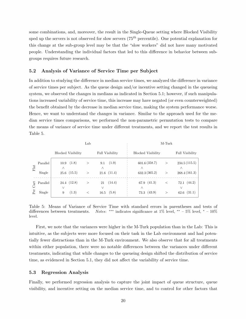
5.2 Analysis of Variance of Service Time per Subject
In addition to studying the difference in median service times, we analyzed the difference in variance
of service times per subject. As the queue design and/or incentive setting changed in the queueing
system, we observed the changes in medians as indicated in Section 5.1; however, if such manipula-
tions increased variability of service time, this increase may have negated (or even counterweighted)
the benefit obtained by the decrease in median service time, making the system performance worse.
Hence, we want to understand the changes in variance. Similar to the approach used for the me-
dian service times comparisons, we performed the non-parametric permutation tests to compare
the means of variance of service time under different treatments, and we report the test results in
Table 5.
Lab M-Turk
Flat
Per
Cart
Blocked Visibility Full Visibility Blocked Visibility Full Visibility
Parallel
Single
Parallel
Single
Lab M-Turk
Flat
Per
Cart
Blocked Visibility Full Visibility Blocked Visibility Full Visibility
Parallel
Single
Parallel
Single
Lab M-Turk
Flat
Per
Cart
Blocked Visibility Full Visibility Blocked Visibility Full Visibility
Parallel
Single
Parallel
Single
Lab M-Turk
Flat
Per
Cart
Blocked Visibility Full Visibility Blocked Visibility Full Visibility
Parallel
Single
Parallel
Single
Lab M-Turk
Flat
Per
Cart
Blocked Visibility Full Visibility Blocked Visibility Full Visibility
Parallel
Single
Parallel
Single
10.9 (1.8)
9.3 (1.8)
4.7 (1.2)
8 (1.6)
12.2 (2.8)
>
<
>
> *
>
>>
<<
>
9.1 (1.9)
10.2 (3.5)
3.6 (0.6)
5.3 (1.1)
9.9 (2.6)
>>
>>
>
601.6 (358.7)
2812.3(1129.4)
5.8 (1.1)
13.5 (3.5)
33.4 (18.2)
>
>
>
>
<
>>
> *
>> *
234.5 (115.5)
907 (380.4)
4.7 (0.8)
10 (5.4)
74.1 (31.2)
>>
>>
<
25.6 (15.5)
81.7 (46.2)
4.1 (0.7)
7.1 (2.1)
13.3 (4.1)
>
>
>
<
>
21.6 (11.4)
63.2 (34)
3.6 (1.1)
7.8 (1.7)
12 (3)
632.3 (365.2)
2816.7(1389.6)
8.7 (1.3)
20.1 (9)
87 (116.5)
>
>
> *
>
>
268.4 (161.3)
1287.5(643.3)
6 (1.5)
12.9 (3.3)
47.9 (18.4)
24.4 (12.8)
82.2 (41.9)
3.3 (0.4)
4.7 (1)
11.5 (3.9)
>
<
>
<
>
<< *
>>
<
21 (14.4)
83.8 (49.3)
3 (0.4)
4.8 (0.9)
7.4 (2)
<<
>>
>
67.9 (41.3)
337.1 (184.3)
3.7 (0.4)
6 (1.6)
20.3 (7.3)
<
>
> *
>
> *
>>
<> *
>
72.1 (44.2)
316.7 (158.6)
2.6 (0.4)
5.3 (0.8)
12.6 (3.5)
<<
>***
> **
> **
9 (1.3)
8.5 (1.4)
3.5 (0.4)
4.9 (1)
11.5 (3)
<
< *
>
>
>
16.5 (5.8)
33.5 (11.8)
3.2 (0.5)
4.8 (1)
10 (5.8)
73.3 (43.9)
359.2 (192.4)
3.4 (1)
9.3 (2.5)
25.5 (7.2)
>
>
< *
<
>
62.6 (31.1)
239 (98.4)
4.8 (0.9)
10.2 (2)
21.4 (4.9)
Table 5: Means of Variance of Service Time with standard errors in parentheses and tests ofdifferences between treatments. Notes: ∗∗∗ indicates significance at 1% level, ∗∗ – 5% level, ∗ – 10%level.
First, we note that the variances were higher in the M-Turk population than in the Lab: This is
intuitive, as the subjects were more focused on their task in the Lab environment and had poten-
tially fewer distractions than in the M-Turk environment. We also observe that for all treatments
within either population, there were no notable differences between the variances under different
treatments, indicating that while changes to the queueing design shifted the distribution of service
time, as evidenced in Section 5.1, they did not affect the variability of service time.
5.3 Regression Analysis
Finally, we performed regression analysis to capture the joint impact of queue structure, queue
visibility, and incentive setting on the median service time, and to control for other factors that
20
could potentially have impacted our results. Since control variables and the variances were different
in the Lab and M-Turk populations, we performed the regression separately for each population.
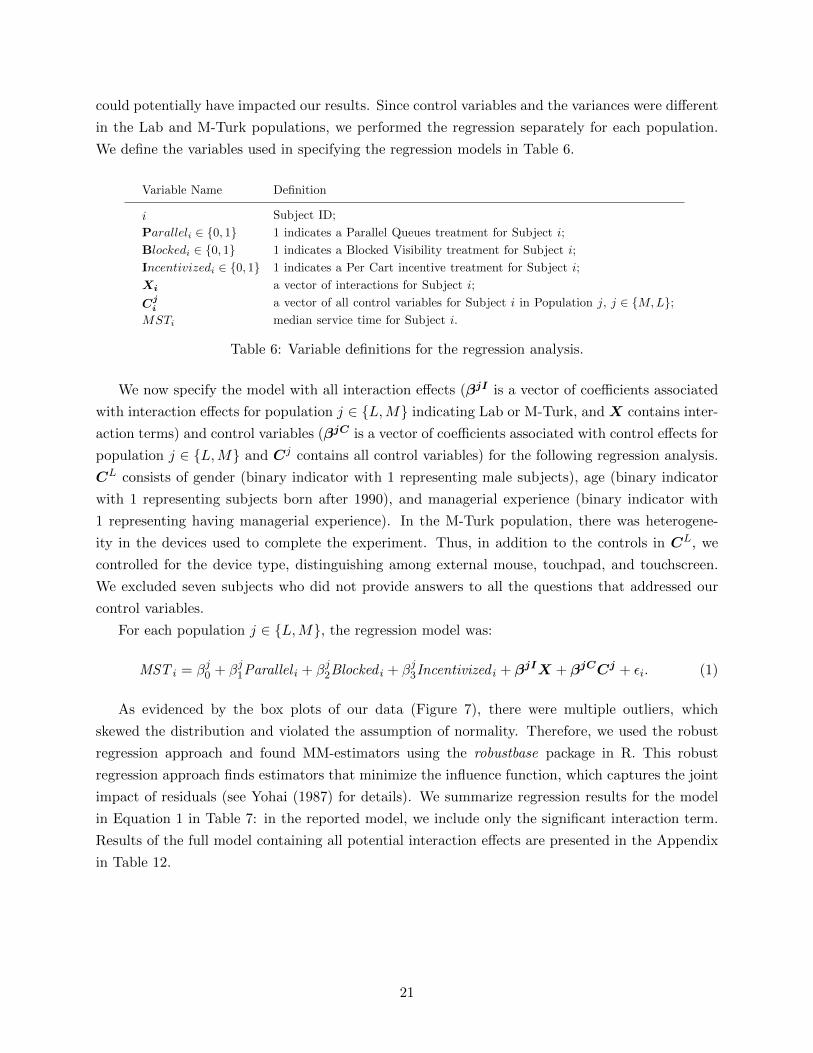
We define the variables used in specifying the regression models in Table 6.
Variable Name
i
Paralleli ∈ {0, 1}Blockedi ∈ {0, 1}Incentivizedi ∈ {0, 1}Xi
Cji
MSTi
Definition
Subject ID;
1 indicates a Parallel Queues treatment for Subject i;
1 indicates a Blocked Visibility treatment for Subject i;
1 indicates a Per Cart incentive treatment for Subject i;
a vector of interactions for Subject i;
a vector of all control variables for Subject i in Population j, j ∈ {M,L};
median service time for Subject i.
Table 6: Variable definitions for the regression analysis.
We now specify the model with all interaction effects (βjI is a vector of coefficients associated
with interaction effects for population j ∈ {L,M} indicating Lab or M-Turk, and X contains inter-
action terms) and control variables (βjC is a vector of coefficients associated with control effects for
population j ∈ {L,M} and Cj contains all control variables) for the following regression analysis.
CL consists of gender (binary indicator with 1 representing male subjects), age (binary indicator
with 1 representing subjects born after 1990), and managerial experience (binary indicator with
1 representing having managerial experience). In the M-Turk population, there was heterogene-
ity in the devices used to complete the experiment. Thus, in addition to the controls in CL, we
controlled for the device type, distinguishing among external mouse, touchpad, and touchscreen.
We excluded seven subjects who did not provide answers to all the questions that addressed our
control variables.
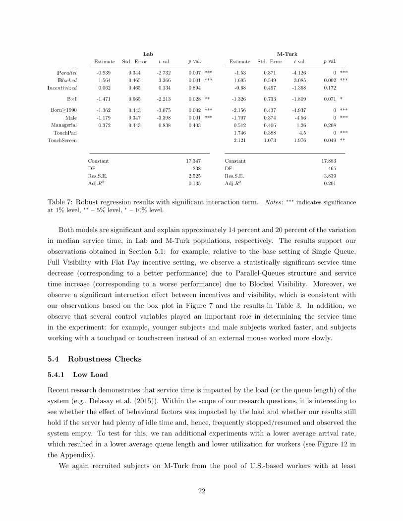
For each population j ∈ {L,M}, the regression model was:
MST i = βj0 + βj1Parallel i + βj2Blocked i + βj3Incentivized i + βjIX + βjCCj + εi. (1)
As evidenced by the box plots of our data (Figure 7), there were multiple outliers, which
skewed the distribution and violated the assumption of normality. Therefore, we used the robust
regression approach and found MM-estimators using the robustbase package in R. This robust
regression approach finds estimators that minimize the influence function, which captures the joint
impact of residuals (see Yohai (1987) for details). We summarize regression results for the model
in Equation 1 in Table 7: in the reported model, we include only the significant interaction term.
Results of the full model containing all potential interaction effects are presented in the Appendix
in Table 12.
21
Lab
Estimate Std. Error t val. p val.
Constant
DF
Res.S.E.
Adj.R2
17.347
238
2.525
0.135
Parallel ***
Blocked ***
Incentivized
-0.939
1.564
0.062
0.344
0.465
0.465
-2.732
3.366
0.134
0.007
0.001
0.894
B×I **-1.471 0.665 -2.213 0.028
Born≥1990 ***
Male ***
Managerial
TouchPad
TouchScreen
-1.362
-1.179
0.372
0.443
0.347
0.443
-3.075
-3.398
0.838
0.002
0.001
0.403
M-Turk
Estimate Std. Error t val. p val.
Constant
DF
Res.S.E.
Adj.R2
17.883
465
3.839
0.201
***
***
-1.53
1.695
-0.68
0.371
0.549
0.497
-4.126
3.085
-1.368
0
0.002
0.172
*-1.326 0.733 -1.809 0.071
-2.156
-1.707
0.512
1.746
2.121
0.437
0.374
0.406
0.388
1.073
-4.937
-4.56
1.26
4.5
1.976
0
0
0.208
0
0.049
***
***
***
**
Table 7: Robust regression results with significant interaction term. Notes: ∗∗∗ indicates significanceat 1% level, ∗∗ – 5% level, ∗ – 10% level.
Both models are significant and explain approximately 14 percent and 20 percent of the variation
in median service time, in Lab and M-Turk populations, respectively. The results support our
observations obtained in Section 5.1: for example, relative to the base setting of Single Queue,
Full Visibility with Flat Pay incentive setting, we observe a statistically significant service time
decrease (corresponding to a better performance) due to Parallel-Queues structure and service
time increase (corresponding to a worse performance) due to Blocked Visibility. Moreover, we
observe a significant interaction effect between incentives and visibility, which is consistent with
our observations based on the box plot in Figure 7 and the results in Table 3. In addition, we
observe that several control variables played an important role in determining the service time
in the experiment: for example, younger subjects and male subjects worked faster, and subjects
working with a touchpad or touchscreen instead of an external mouse worked more slowly.
5.4 Robustness Checks
5.4.1 Low Load
Recent research demonstrates that service time is impacted by the load (or the queue length) of the
system (e.g., Delasay et al. (2015)). Within the scope of our research questions, it is interesting to
see whether the effect of behavioral factors was impacted by the load and whether our results still
hold if the server had plenty of idle time and, hence, frequently stopped/resumed and observed the
system empty. To test for this, we ran additional experiments with a lower average arrival rate,
which resulted in a lower average queue length and lower utilization for workers (see Figure 12 in
the Appendix).
We again recruited subjects on M-Turk from the pool of U.S.-based workers with at least
22
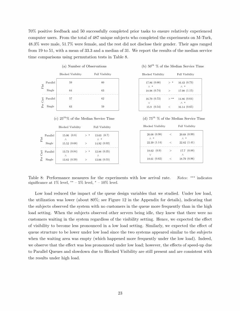
70% positive feedback and 50 successfully completed prior tasks to ensure relatively experienced
computer users. From the total of 487 unique subjects who completed the experiments on M-Turk,
48.3% were male, 51.7% were female, and the rest did not disclose their gender. Their ages ranged
from 19 to 51, with a mean of 33.3 and a median of 31. We report the results of the median service
time comparisons using permutation tests in Table 8.
(a) Number of ObservationsM-Turk: Low
Flat
Per
Cart
Blocked Visibility Full Visibility
Parallel
Single
Parallel
Single
59 60
64 63
57 62
63 59
(b) 50th % of the Median Service Time
M-Turk: Low
Flat
Per
Cart
Blocked Visibility Full Visibility
Parallel
Single
Parallel
Single
M-Turk: Low
Flat
Per
Cart
Blocked Visibility Full Visibility
Parallel
Single
Parallel
Single
M-Turk: Low
Flat
Per
Cart
Blocked Visibility Full Visibility
Parallel
Single
Parallel
Single
M-Turk: Low
Flat
Per
Cart
Blocked Visibility Full Visibility
Parallel
Single
Parallel
Single
M-Turk: LowFlat
Per
Cart
Blocked Visibility Full Visibility
Parallel
Single
Parallel
Single
18.33 (0.68)
5.21 (0.74)
15.06 (0.8)
17.86 (0.66)
20.08 (0.98)
<
< *
> *
> *
<
><
>> *
> *
19.89 (1.94)
15.04 (5.31)
13.63 (0.7)
16.43 (0.73)
20.68 (0.99)
<<
> *
> *
> *
19.34 (0.57)
4.44 (0.34)
15.52 (0.68)
18.98 (0.74)
22.39 (1.14)
<
<***
>
>
<
19.77 (0.86)
7.08 (0.95)
14.92 (0.92)
17.98 (1.15)
22.82 (1.41)
16.93 (0.61)
4.59 (0.65)
13.73 (0.84)
16.79 (0.72)
18.62 (0.9)
> *
>
> *
> **
>
<<
><
<
15.57 (0.52)
4.28 (0.46)
12.88 (0.35)
14.86 (0.64)
17.7 (0.88)
> *
>>
> *
>
16.67 (0.55)
4.29 (0.66)
13.82 (0.59)
15.9 (0.54)
18.61 (0.62)
<
<
>
<
<
16.8 (0.69)
5.42 (0.82)
13.06 (0.55)
16.14 (0.65)
18.79 (0.96)
(c) 25th% of the Median Service Time
M-Turk: Low
Flat
Per
Cart
Blocked Visibility Full Visibility
Parallel
Single
Parallel
Single
M-Turk: Low
Flat
Per
Cart
Blocked Visibility Full Visibility
Parallel
Single
Parallel
Single
M-Turk: Low
Flat
Per
Cart
Blocked Visibility Full Visibility
Parallel
Single
Parallel
Single
M-Turk: Low
Flat
Per
Cart
Blocked Visibility Full Visibility
Parallel
Single
Parallel
Single
M-Turk: Low
Flat
Per
Cart
Blocked Visibility Full Visibility
Parallel
Single
Parallel
Single
18.33 (0.68)
5.21 (0.74)
15.06 (0.8)
17.86 (0.66)
20.08 (0.98)
<
< *
> *
> *
<
><
>> *
> *
19.89 (1.94)
15.04 (5.31)
13.63 (0.7)
16.43 (0.73)
20.68 (0.99)
<<
> *
> *
> *
19.34 (0.57)
4.44 (0.34)
15.52 (0.68)
18.98 (0.74)
22.39 (1.14)
<
<***
>
>
<
19.77 (0.86)
7.08 (0.95)
14.92 (0.92)
17.98 (1.15)
22.82 (1.41)
16.93 (0.61)
4.59 (0.65)
13.73 (0.84)
16.79 (0.72)
18.62 (0.9)
> *
>
> *
> **
>
<<
><
<
15.57 (0.52)
4.28 (0.46)
12.88 (0.35)
14.86 (0.64)
17.7 (0.88)
> *
>>
> *
>
16.67 (0.55)
4.29 (0.66)
13.82 (0.59)
15.9 (0.54)
18.61 (0.62)
<
<
>
<
<
16.8 (0.69)
5.42 (0.82)
13.06 (0.55)
16.14 (0.65)
18.79 (0.96)
(d) 75th % of the Median Service Time
M-Turk: Low
Flat
Per
Cart
Blocked Visibility Full Visibility
Parallel
Single
Parallel
Single
M-Turk: Low
Flat
Per
Cart
Blocked Visibility Full Visibility
Parallel
Single
Parallel
Single
M-Turk: Low
Flat
Per
Cart
Blocked Visibility Full Visibility
Parallel
Single
Parallel
Single
M-Turk: Low
Flat
Per
Cart
Blocked Visibility Full Visibility
Parallel
Single
Parallel
Single
M-Turk: Low
Flat
Per
Cart
Blocked Visibility Full Visibility
Parallel
Single
Parallel
Single
18.33 (0.68)
5.21 (0.74)
15.06 (0.8)
17.86 (0.66)
20.08 (0.98)
<
< *
> *
> *
<
><
>> *
> *
19.89 (1.94)
15.04 (5.31)
13.63 (0.7)
16.43 (0.73)
20.68 (0.99)
<<
> *
> *
> *
19.34 (0.57)
4.44 (0.34)
15.52 (0.68)
18.98 (0.74)
22.39 (1.14)
<
<***
>
>
<
19.77 (0.86)
7.08 (0.95)
14.92 (0.92)
17.98 (1.15)
22.82 (1.41)
16.93 (0.61)
4.59 (0.65)
13.73 (0.84)
16.79 (0.72)
18.62 (0.9)
> *
>
> *
> **
><
<>
<<
15.57 (0.52)
4.28 (0.46)
12.88 (0.35)
14.86 (0.64)
17.7 (0.88)
> *
>>
> *
>
16.67 (0.55)
4.29 (0.66)
13.82 (0.59)
15.9 (0.54)
18.61 (0.62)
<
<
>
<
<
16.8 (0.69)
5.42 (0.82)
13.06 (0.55)
16.14 (0.65)
18.79 (0.96)
Table 8: Performance measures for the experiments with low arrival rate. Notes: ∗∗∗ indicatessignificance at 1% level, ∗∗ – 5% level, ∗ – 10% level.
Low load reduced the impact of the queue design variables that we studied. Under low load,
the utilization was lower (about 80%; see Figure 12 in the Appendix for details), indicating that
the subjects observed the system with no customers in the queue more frequently than in the high
load setting. When the subjects observed other servers being idle, they knew that there were no
customers waiting in the system regardless of the visibility setting. Hence, we expected the effect
of visibility to become less pronounced in a low load setting. Similarly, we expected the effect of
queue structure to be lower under low load since the two systems appeared similar to the subjects
when the waiting area was empty (which happened more frequently under the low load). Indeed,
we observe that the effect was less pronounced under low load; however, the effects of speed-up due
to Parallel Queues and slowdown due to Blocked Visibility are still present and are consistent with
the results under high load.
23
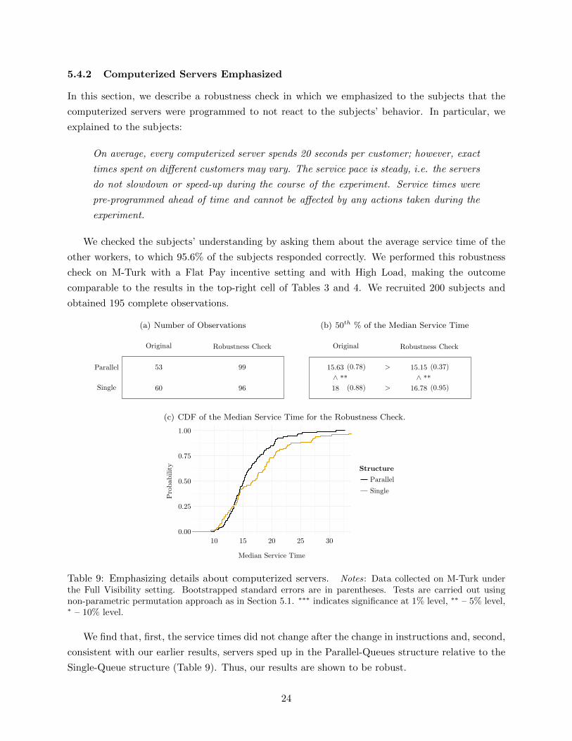
5.4.2 Computerized Servers Emphasized
In this section, we describe a robustness check in which we emphasized to the subjects that the
computerized servers were programmed to not react to the subjects’ behavior. In particular, we
explained to the subjects:
On average, every computerized server spends 20 seconds per customer; however, exact
times spent on different customers may vary. The service pace is steady, i.e. the servers
do not slowdown or speed-up during the course of the experiment. Service times were
pre-programmed ahead of time and cannot be affected by any actions taken during the
experiment.
We checked the subjects’ understanding by asking them about the average service time of the
other workers, to which 95.6% of the subjects responded correctly. We performed this robustness
check on M-Turk with a Flat Pay incentive setting and with High Load, making the outcome
comparable to the results in the top-right cell of Tables 3 and 4. We recruited 200 subjects and
obtained 195 complete observations.
(a) Number of ObservationsM-Turk: Full Visibility
Flat
Original Robustness Check
Parallel
Single
St.dev.
M-Turk
Flat
Original Robustness Check
Parallel
Single
25th perc.
M-Turk
Flat
Original Robustness Check
Parallel
Single
M-Turk: Full Visibility
Flat
Original Robustness Check
Parallel
Single
75th perc.
M-Turk
Flat
Original Robustness Check
Parallel
Single
53
6.61 (1.14)
13.23 (0.47)
15.63 (0.78)
19.79 (1.19)
> **
<
>
> *
< **
> *
> **
>
99
3.81 (0.4)
13.45 (0.29)
15.15 (0.37)
17.88 (0.7)
>***
<> **
>***
60
4.2 (0.26)
14.35 (0.79)
18 (0.88)
21.79 (0.76)
<***
> *
>
>
96
12.79 (4.94)
13.35 (0.56)
16.78 (0.95)
20.41 (0.78)
(b) 50th % of the Median Service Time
M-Turk: Full Visibility
Flat
Original Robustness Check
Parallel
Single
St.dev.
M-Turk
Flat
Original Robustness Check
Parallel
Single
25th perc.
M-Turk
Flat
Original Robustness Check
Parallel
Single
M-Turk: Full Visibility
Flat
Original Robustness Check
Parallel
Single
75th perc.
M-Turk
Flat
Original Robustness Check
Parallel
Single
53
6.61 (1.14)
13.23 (0.47)
15.63 (0.78)
19.79 (1.19)
> **
<
>
> *
< **
> *
> **
>
99
3.81 (0.4)
13.45 (0.29)
15.15 (0.37)
17.88 (0.7)
>***
<> **
>***
60
4.2 (0.26)
14.35 (0.79)
18 (0.88)
21.79 (0.76)
<***
> *
>
>
96
12.79 (4.94)
13.35 (0.56)
16.78 (0.95)
20.41 (0.78)
(c) CDF of the Median Service Time for the Robustness Check.
0.00
0.25
0.50
0.75
1.00
10 15 20 25 30
Median Service Time
Pro
babi
lity Structure
Parallel
Single
Table 9: Emphasizing details about computerized servers. Notes: Data collected on M-Turk underthe Full Visibility setting. Bootstrapped standard errors are in parentheses. Tests are carried out usingnon-parametric permutation approach as in Section 5.1. ∗∗∗ indicates significance at 1% level, ∗∗ – 5% level,∗ – 10% level.
We find that, first, the service times did not change after the change in instructions and, second,
consistent with our earlier results, servers sped up in the Parallel-Queues structure relative to the
Single-Queue structure (Table 9). Thus, our results are shown to be robust.
24
6 Conclusion
The results of our study indicate that the physical layout of the service environment can influence
worker effort and, hence, the system’s overall performance. Specifically, we show that the median
service time is higher in single-queue structures than in parallel-queues. From a managerial stand-
point, when choosing to transition to single-queue structures, one has to be aware of the potential
slowdown of servers; otherwise, the managers can overestimate the increase in performance after
the move and fail to meet service goals.
We show that the behavioral mechanism that causes this slowdown depends on the payment
scheme. In queueing systems in which servers are compensated regardless of their performance
(flat pay incentive setting), the slowdown of servers is driven by task interdependence. In practice,
this implies that in order to prevent (or mitigate) this slowdown, the managers have to focus
on decreasing the task interdependence or decreasing effort dispensability. In queueing systems
in which servers are compensated for performance (per cart incentive setting), the slowdown is
driven by the feedback availability. Thus, to mitigate the slowdown, the managers have to focus
on increasing feedback (for example, by providing real-time information about the queue to the
servers or explicitly monitoring individual performances).
Within each structure, queue visibility plays an important role: in most settings, blocked visi-
bility increases service time (decreasing performance); hence, managers of such systems may want
to manipulate feedback to improve performance. Improvement of feedback can come from adjusting
the physical layout of the queue to reduce visibility barriers (e.g., lowering the height of display
cases) or adding visibility enhancements (e.g., mirrors or video displays of the line or electronic
displays of customer movement within the store). However, when servers are compensated for per-
formance (per cart incentive setting) in the single-queue structure, blocking visibility may lead to
improved performance.
Across the literature on worker behavior and queueing theory, we have explored the separate ef-
fects of feedback and task interdependence as drivers of performance for parallel and single queues.
These findings add to the body of work on the impact of the work environment on employees’ be-
havior. More specifically, within the queueing theory literature, we consider non-discretionary tasks
across environmental factors. To isolate feedback and interdependence as the variables of interest,
we have controlled for many additional factors, including group size, interpersonal dynamics, cart
complexities, and relative speed of co-workers. Incorporating these real-world complexities into the
future research would further enrich the understanding of how output and performance are driven
by the physical and personal design of work teams.
Finally, the impact of worker slowdown on customer satisfaction requires further analysis. Over-
all, the slower worker speed under single queues or low visibility may result in lower customer
satisfaction, but not necessarily. In settings in which customers are not concerned about speed,
but, rather, prefer a slower and more-personalized service, the result of server slowdown may lead
to an increase in customer satisfaction. This area of research, as proposed by Bendoly et al. (2010),
requires further investigation. Another important consideration in selecting the queue structure
25
is fairness as perceived by customers: social justice would favor single-queue systems due to the
first-come-first-serve order of serving customers. Exploring customer perceptions regarding queue
structure and corresponding changes in service time also requires further study.
26
References
Alnuaimi, O. A., L. P. Robert, L. M. Maruping. 2010. Team size, dispersion, and social loafing in technology-
supported teams: A perspective on the theory of moral disengagement. Journal of Management Informa-
tion Systems 27(1) 203–230.
Anand, K. S., M Fazıl Pac, S. Veeraraghavan, et al. 2011. Quality–speed conundrum: Tradeoffs in customer-
intensive services. Management Science 57(1) 40–56.
Bandiera, O., I. Barankay, I. Rasul. 2010. Social incentives in the workplace. The Review of Economic
Studies 77(2) 417–458.
Bendoly, E., R. Croson, P. Goncalves, K. L Schutlz. 2010. Bodies of knowledge for research in behavioral
operations. Production and Operations Management 19(4) 434–452.
Berinsky, A. J., G. A. Huber, G. S. Lenz. 2012. Evaluating online labor markets for experimental research:
Amazon.com’s Mechanical Turk. Political Analysis 20(3) 351–368.
Buhrmester, M, T. Kwang, S. D. Gosling. 2011. Amazon’s Mechanical Turk: A new source of inexpensive,
yet high-quality, data? Perspectives on Psychological Science 6(3) 3–5.
Cachon, G., F. Zhang. 2007. Obtaining fast service in a queueing system via performance-based allocation
of demand. Management Science 53(3) 408–420.
Debo, L., B. Toktay, L. N. Van Wassenhove. 2008. Queueing for expert services. Management Science 54(8)
1497–1512.
Delasay, M., A. Ingolfsson, B. Kolfal, K. Schultz. 2015. Load effect on service times. Working Paper.
Donovan, J. J. 2001. Work motivation. N. Anderson, D. S. Ones, H. K. Sinangil, C. Viswesvaran, eds.,
Handbook of Industrial work and Organizational Psychology , vol. 2. Sage, London, 53–76.
Erez, M. 1977. Feedback: A necessary condition for the goal setting-performance relationship. Journal of
Applied Psychology 62(5) 624.
Ernst, M. D. 2004. Permutation methods: a basis for exact inference. Statistical Science 19(4) 676–685.
Fantasia, R. 2009. Move up to the head of the line: Hannaford market tests managing cart traffic at the
register. TimesUnion.com. 1 August, 2009.
Fisher, R.A. 1935. The Design of Experiments. 3rd ed. Oliver & Boyd, London.
Gilbert, S. M., Z. K. Weng. 1998. Incentive effects favor nonconsolidating queues in a service system: The
principal–agent perspective. Management Science 44(12) 1662–1669.
Gill, D., V. L. Prowse. 2011. A novel computerized real effort task based on sliders. Working Paper, Econstor.
Good, P. 2013. Permutation tests: a practical guide to resampling methods for testing hypotheses. Springer
Science & Business Media.
Goodman, J. K., C. E. Cryder, A. Cheema. 2012. Data collection in a flat world: The strengths and
weaknesses of Mechanical-Turk samples. Journal of Behavioral Decision Making 26 213–224.
27
Hasija, S., E. Pinker, R. A. Shumsky. 2010. Work expands to fill the time available: Capacity estimation
and staffing under Parkinson’s law. Manufacturing & Service Operations Management 12(1) 1–18.
Hauss, D. 2008. Queue science helps retailers recover revenue at checkout. RetailTouchpoints.com. 8 August,
2008.
Helms, M. 2011. Minneapolis Target store’s new checkout system ‘test’ raises customer hackles – and
questions. MinnPost.com. 22 November 2011.
Hopp, W. J., S. Iravani, F. Liu. 2009. Managing white-collar work: An operations-oriented survey. Production
and Operations Management 18(1) 1–32.
Hopp, W. J., S. Iravani, G. Y. Yuen. 2007. Operations systems with discretionary task completion. Man-
agement Science 53(1) 61–77.
Horton, J., L. Chilton. 2010. The labor economics of paid crowdsourcing. Proceedings of the 11th ACM
Conference on Electronic Commerce. EC ’10, ACM, New York, NY, USA, 209–218.
Horton, J. J, D. G Rand, R. J Zeckhauser. 2011. The online laboratory: conducting experiments inareal-
labormarket. Experimental Economics 14(3) 399–425.
Hossain, T., J. A List. 2012. The behavioralist visits the factory: Increasing productivity using simple
framing manipulations. Management Science 58(12) 2151–2167.
Jones, G. R. 1984. Task visibility, free riding, and shirking: Explaining the effect of structure and technology
on employee behavior. Academy of Management Review 9(4) 684–695.
Jouini, O., Y. Dallery, R. Nait-Abdallah. 2008. Analysis of the impact of team-based organizations in call
center management. Management Science 54(2) 400–414.
Joustra, P. E., E. Van der Sluis, N. M. Van Dijk. 2010. To pool or not to pool in hospitals: a theoretical and
practical comparison for a radiotherapy outpatient department. Annals of Operations Research 178(1)
77–89.
Karau, S. J., K. D. Williams. 1993. Social loafing: A meta-analytic review and theoretical integration.
Journal of Personality and Social Psychology 65(4) 681–706.
Kidwell, R. E., N. Bennett. 1993. Employee propensity to withhold effort: A conceptual model to intersect
three avenues of research. Academy of management review 18(3) 429–456.
Latham, G. P., E. A. Locke. 1991. Self-regulation through goal setting. Organizational behavior and human
decision processes 50(2) 212–247.
Mas, A., E. Moretti. 2009. Peers at work. American Economic Review 99(1) 112–145.
Oliva, R., J. D. Sterman. 2001. Cutting corners and working overtime: Quality erosion in the service industry.
Management Science 47(7) 894–914.
Paolacci, G., J. Chandler, P. G. Ipeirotis. 2010. Running experiments on Amazon Mechanical Turk. Judgment
and Decision Making 5(5) 411–419.
28
Pearce, J. L., H. B. Gregersen. 1991. Task interdependence and extrarole behavior: A test of the mediating
effects of felt responsibility. Journal of Applied Psychology 76(6) 838.
Phipson, B., G. K. Smyth. 2010. Permutation p-values should never be zero: calculating exact p-values when
permutations are randomly drawn. Statistical applications in genetics and molecular biology 9(1).
Powell, S. G., K. L. Schultz. 2004. Throughput in serial lines with state-dependent behavior. Management
Science 50(8) 1095–1105.
Rand, D. G. 2012. The promise of Mechanical Turk: How online labor markets can help theorists run
behavioral experiments. Journal of Theoretical Biology 299 172 – 179.
Schultz, K. L, D. C Juran, J. W Boudreau. 1999. The effects of low inventory on the development of
productivity norms. Management Science 45(12) 1664–1678.
Schultz, K. L, D. C Juran, J. W Boudreau, J. O McClain, J. L Thomas. 1998. Modeling and worker
motivation in JIT production systems. Management Science 44(12-part-1) 1595–1607.
Schultz, K. L., J. O. McClain, J. L. Thomas. 2003. Overcoming the dark side of worker flexibility. Journal
of Operations Management 21(1) 81–92.
Schultz, K. L., T. Schoenherr, D. Nembhard. 2010. An example and a proposal concerning the correlation
of worker processing times in parallel tasks. Management Science 56(1) 176–191.
Song, H., A. Tucker, K. L. Murrell. 2015. The diseconomies of queue pooling: An empirical investigation of
emergency department length of stay. Management Science 61(12) 3032–3053.
Tan, F., S. Netessine. 2014. The implications of worker behavior for staffing decisions: Empirical evidence
and best practices. Cornell Hospitality Quarterly forthcoming.
Wang, J., Y. Zhou. 2015. Social loafing and queue driven speedup: Evidence from a supermarket. Working
Paper.
Wickelgren, W. A. 1977. Speed–accuracy tradeoff and information processing dynamics. Acta Psychologica
41 67–85.
Williams, K., S. G Harkins, B. Latane. 1981. Identifiability as a deterrant to social loafing: Two cheering
experiments. Journal of Personality and Social Psychology 40(2) 303.
Williamson, O. E. 1975. Markets and hierarchies. New York 26–30.
Yohai, V. J. 1987. High breakdown-point and high efficiency robust estimates for regression. The Annals of
Statistics 15(2) 642–656.
29
7 Appendix
7.1 Experimental Instructions
Welcome: “Thank you for your participation today. This task should take 20 minutes. You will earn [X]
for your time today. Your responses will be used to do academic research. We appreciate you taking your
time and giving this your full consideration.” Subjects then create a unique user ID. Consent is confirmed.
Next, subjects are asked to fill out a questionnaire, which includes questions about managerial experience,
gender, age, marital status, children, education, time in the United States, and input device type.
Training: “You will be completing a 2 minute training period on the next screen.” Subjects are presented
with the animated training screen. “This is an individual task which will give you practice before you
participate in the study task in later screens.”
“You will be acting as a cashier in a grocery store. Your customers each have five items in their cart. To
process a customer’s order, slide each bar to match the listed price. Once all items are entered, click submit
button to move to the next cart. The “Submit Cart” button will remain inactive until you correctly set all 5
prices. This training period is to ensure you can do the mechanics of the task on your machine. The screen
will auto-advance after 2 minutes.” Upon completion, subjects verify that training screens loaded. If they do
not, they can repeat training.
Task Instructions: Instructions for each treatment follow.
Per Cart treatment: “The training period is complete. The actual task is about to begin. You will earn
[rate] for each customer that you successfully submit. Thus if you complete 10 customers, you will earn
[bonus] in addition to the [flat payment]. Please indicate that you read the following by correctly answering:
If you complete X carts, how much will you earn as a bonus?” Forced response.
Flat Pay: “That completes your training on the software. You will now work a ten minute shift in the
grocery store. When the shift is over you will be asked several questions about your experience. ”
M-Turk: “Then you will receive a completion code to submit to M-Turk to claim payment.”
Lab: “Then you will get a printed receipt for payment.”
Parallel: “Reminder, the task will last 10 minutes, and when it is over you will be asked several questions
about your experience. You will now be working in a group with 3 other computerized servers. As customers
arrive to the checkout area, they choose the line that currently has the fewest customers and wait in that
line. Each server has his or her own line.”
Single: “Reminder, the task will last 10 minutes, and when it is over you will be asked several questions
about your experience. You will now be working in a group with 3 other computerized servers. As customers
arrive to the checkout area, they join a single group line and then go to the next available server when their
turn comes.”
Blocked Visibility: “You can see part, but not all of the line as it wraps behind a fence.”
All: “You will be awarded your payment upon completion of one 10 minute shift and some short
surveys. Please answer the following questions to indicate your understanding” Subjects are presented with
an animated sample screen. Next, subjects are asked questions about how the customers wait in line and
number of co-workers.
Exit Surveys: Subjects were then assessed for questions of self-efficacy, group cohesion and perception,
locus-of-control, as well as manipulation checks regarding the number of servers, the type of co-workers
(human or computerized), queue structure, items per cart, and their perception of relative service time.
30
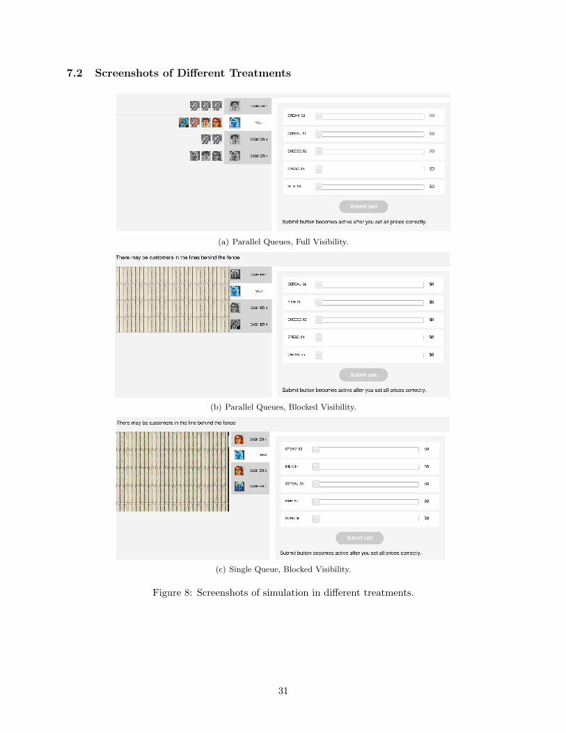
7.2 Screenshots of Different Treatments
(a) Parallel Queues, Full Visibility.
(b) Parallel Queues, Blocked Visibility.
(c) Single Queue, Blocked Visibility.
Figure 8: Screenshots of simulation in different treatments.
31
7.3 Supplemental Figures
0.00
0.25
0.50
0.75
1.00
10 20 30
Service Time
Pro
babi
lity
Figure 9: Empirical distribution of service times from a pilot study. Notes: The pilot was conductedin the lab and involved a four-server setup similar to that in the current experiment. Empirical distributionis solid black. Dashed Red is the distribution associated with a service time of ten plus an exponentialrandom variable with a mean of ten. The red dashed line represents the distribution of service times usedfor the computerized servers.
Lab M.Turk
0
25
50
75
100
-2 0 2 -2 0 2Theoretical Quantiles
Sam
ple
Qua
ntile
s
Figure 10: Q-Q Plot of Median Service Time
32
Single Queue Parallel Queues
0.0
2.5
5.0
7.5
10.0
0 200 400 600 0 200 400 600
Seconds
Que
ue L
engt
h Average Service Time
24
20
16
Figure 11: Average queue length during the ten-minute service interval for the low load. Notes:Queue length averaged across 500 simulations of a ten-minute interval. Service times of the three computerservers are fixed at ten plus an exponential random variable with a mean of ten. The Average Service Timeof the fourth server is varied, assuming the same additive structure, to investigate the possible effect of thebehavioral server with different service time on the queue length. For example, the service time of 16 inthis figure corresponds to ten plus an exponential random variable with a mean of six. Customers arrivedaccording to an exponential random variable with a mean of 6.5. Single queue was initialized with onecustomer at each server and three customers in the pooled queue. The queue-length variable for the singlequeue measures the average number of customers in the pooled queue. Parallel queues was initialized withone customer at each server and two customers in each queue. The queue-length variable for the parallelqueues measures the average number of customers in the line in front of the simulated behavioral agent.
33
Single Queue Parallel Queues
0.00
0.25
0.50
0.75
1.00
0 200 400 600 0 200 400 600
Seconds
Utilization
Average Service Time
24
20
16
(a) High Load
Single Queue Parallel Queues
0.00
0.25
0.50
0.75
1.00
0 200 400 600 0 200 400 600
Seconds
Utilization
Average Service Time
24
20
16
(b) Low Load
Figure 12: Average server utilization during the ten-minute service interval. Notes: Server utilizationaveraged across 500 simulations of a ten-minute interval. Service times of the three computerized servers arefixed at ten plus an exponential random variable with mean of ten. The Average Service Time of the fourthserver is varied, assuming the same additive structure, to investigate possible effect of a human server withdifferent service times on the utilization. For example, the service time of 16 in this figure corresponds toten plus an exponential random variable with mean of six. The Utilization variable measures the averageutilization of the simulated human agent. (a) Customers arrive according to an exponential random variablewith a mean of 5.5. Single queue starts with one customer at each server and eight customers in the pooledqueue. Parallel queues start with one customer at each server and three customers in each queue. (b)Customers arrive according to an exponential random variable with a mean of 6.5. Single queue startswith one customer at each server and three customers in the pooled queue. Parallel queues start with onecustomer at each server and two customers in each queue.
34
Parallel Queues
0
1
2
3
4
5
0 200 400 600
Seconds
Que
ue L
engt
h Customers' Queue-joining Behavior
Join Random Queue
Join Shortest Queue
Jockeying
Figure 13: Average queue length depending on customers’ queue-joining behavior. Notes: Queuelength averaged across 500 simulations of a ten-minute interval for the high load setting. Service times ofthe three computerized servers are fixed at ten plus an exponential random variable with a mean of ten.The service time of the fourth server is also fixed, assuming the same additive structure, at ten plus anexponential random variable with a mean of six. Customers arrive according to an exponential randomvariable with a mean of 5.5. Parallel queues start with one customer at each server and three customers ineach queue. The Queue Length variable for the parallel queues measures the average number of customersin the line in front of the simulated behavioral agent, depending on the queue-joining behavior.
7.4 Supplemental Tables
7.4.1 Robustness Check: Average Service Time
For robustness, we perform our means and 50th percentile comparison tests using Average Service Time
measure:
35
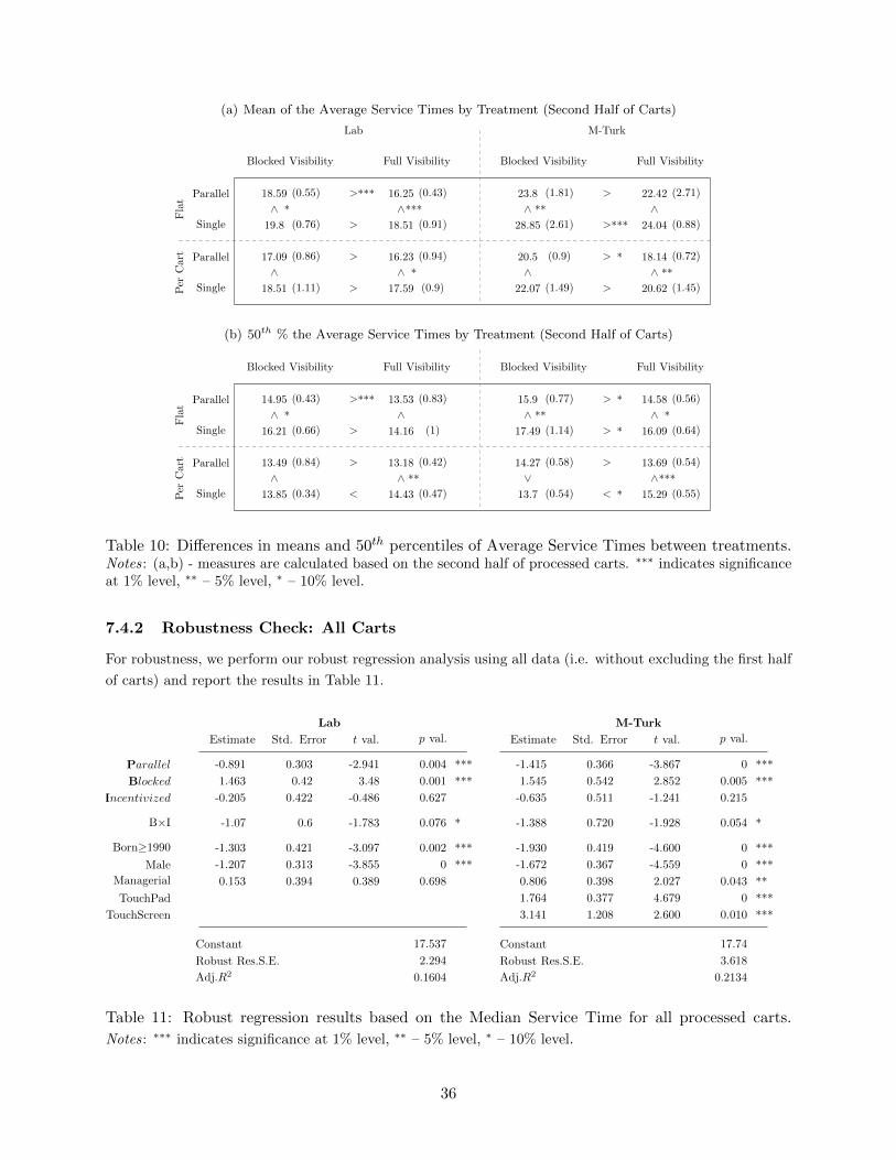
(a) Mean of the Average Service Times by Treatment (Second Half of Carts)
Lab M-Turk
Flat
Per
Cart
Blocked Visibility Full Visibility Blocked Visibility Full Visibility
Parallel
Single
Parallel
Single
Lab M-Turk
Flat
Per
Cart
Blocked Visibility Full Visibility Blocked Visibility Full Visibility
Parallel
Single
Parallel
Single
Lab M-Turk
Flat
Per
Cart
Blocked Visibility Full Visibility Blocked Visibility Full Visibility
Parallel
Single
Parallel
Single
Lab M-Turk
Flat
Per
Cart
Blocked Visibility Full Visibility Blocked Visibility Full Visibility
Parallel
Single
Parallel
Single
Lab M-Turk
Flat
Per
Cart
Blocked Visibility Full Visibility Blocked Visibility Full Visibility
Parallel
Single
Parallel
Single
16.95 (0.45)
2.43 (0.33)
14.95 (0.43)
16.98 (0.78)
18.59 (0.55)
>***
<
>***
>***
>***
> **
>> *
> *
> *
15.1 (0.5)
2.7 (0.5)
13.53 (0.83)
15.29 (0.47)
16.25 (0.43)
> **
>>
> **
>***
22.46 (1.67)
12.64 (3.19)
15.9 (0.77)
19.16 (0.87)
23.8 (1.81)
>
>
> *
> **
>
> **
>> **
> **
> **
20.17 (1.11)
8.24 (1.15)
14.58 (0.56)
16.88 (0.9)
22.42 (2.71)
><
> *
> *
>
18.52 (0.83)
4.31 (1.23)
16.21 (0.66)
18.34 (0.84)
19.8 (0.76)
>
>
>
>
>
16.99 (0.8)
4.24 (1.05)
14.16 (1)
16.92 (0.67)
18.51 (0.91)
27.84 (2.65)
21.37 (5.43)
17.49 (1.14)
21.26 (1.11)
28.85 (2.61)
>***
> **
> *
> *
>***
20.4 (0.9)
7.14 (1.5)
16.09 (0.64)
19.1 (0.96)
24.04 (0.88)
16.52 (0.91)
5.55 (1.52)
13.49 (0.84)
15.59 (0.41)
17.09 (0.86)
>
>
>
> *
>
<<
><
>
15.15 (0.53)
3.01 (0.6)
13.18 (0.42)
14.26 (0.56)
16.23 (0.94)
> **
>> **
>***
> *
18.68 (0.94)
7.58 (1.55)
14.27 (0.58)
16.69 (0.67)
20.5 (0.9)
>
>
>
>
> *
><
<>
>
17.39 (0.98)
7.53 (1.59)
13.69 (0.54)
15.61 (0.64)
18.14 (0.72)
> **
>>***
>***
> **
15.97 (0.46)
2.96 (0.25)
13.85 (0.34)
15.09 (0.59)
18.51 (1.11)
<
<
<
< *
>
16.75 (0.57)
3.34 (0.5)
14.43 (0.47)
16.3 (0.49)
17.59 (0.9)
18.76 (0.83)
6.82 (0.99)
13.7 (0.54)
16.76 (0.83)
22.07 (1.49)
<
<
< *
<
>
20.43 (1.45)
10.86 (3.37)
15.29 (0.55)
18.55 (1.05)
20.62 (1.45)
(b) 50th % the Average Service Times by Treatment (Second Half of Carts)
Lab M-Turk
Flat
Per
Cart
Blocked Visibility Full Visibility Blocked Visibility Full Visibility
Parallel
Single
Parallel
Single
Lab M-Turk
Flat
Per
Cart
Blocked Visibility Full Visibility Blocked Visibility Full Visibility
Parallel
Single
Parallel
Single
Lab M-Turk
Flat
Per
Cart
Blocked Visibility Full Visibility Blocked Visibility Full Visibility
Parallel
Single
Parallel
Single
Lab M-Turk
Flat
Per
Cart
Blocked Visibility Full Visibility Blocked Visibility Full Visibility
Parallel
Single
Parallel
Single
Lab M-Turk
Flat
Per
Cart
Blocked Visibility Full Visibility Blocked Visibility Full Visibility
Parallel
Single
Parallel
Single
16.95 (0.45)
2.43 (0.33)
14.95 (0.43)
16.98 (0.78)
18.59 (0.55)
>***
<
>***
>***
>***
> **
>> *
> *
> *
15.1 (0.5)
2.7 (0.5)
13.53 (0.83)
15.29 (0.47)
16.25 (0.43)
> **
>>
> **
>***
22.46 (1.67)
12.64 (3.19)
15.9 (0.77)
19.16 (0.87)
23.8 (1.81)
>
>
> *
> **
>
> **
>> **
> **
> **
20.17 (1.11)
8.24 (1.15)
14.58 (0.56)
16.88 (0.9)
22.42 (2.71)
><
> *
> *
>
18.52 (0.83)
4.31 (1.23)
16.21 (0.66)
18.34 (0.84)
19.8 (0.76)
>
>
>
>
>
16.99 (0.8)
4.24 (1.05)
14.16 (1)
16.92 (0.67)
18.51 (0.91)
27.84 (2.65)
21.37 (5.43)
17.49 (1.14)
21.26 (1.11)
28.85 (2.61)
>***
> **
> *
> *
>***
20.4 (0.9)
7.14 (1.5)
16.09 (0.64)
19.1 (0.96)
24.04 (0.88)
16.52 (0.91)
5.55 (1.52)
13.49 (0.84)
15.59 (0.41)
17.09 (0.86)
>
>
>
> *
>
<<
><
>
15.15 (0.53)
3.01 (0.6)
13.18 (0.42)
14.26 (0.56)
16.23 (0.94)
> **
>> **
>***
> *
18.68 (0.94)
7.58 (1.55)
14.27 (0.58)
16.69 (0.67)
20.5 (0.9)
>
>
>
>
> *
><
<>
>
17.39 (0.98)
7.53 (1.59)
13.69 (0.54)
15.61 (0.64)
18.14 (0.72)
> **
>>***
>***
> **
15.97 (0.46)
2.96 (0.25)
13.85 (0.34)
15.09 (0.59)
18.51 (1.11)
<
<
<
< *
>
16.75 (0.57)
3.34 (0.5)
14.43 (0.47)
16.3 (0.49)
17.59 (0.9)
18.76 (0.83)
6.82 (0.99)
13.7 (0.54)
16.76 (0.83)
22.07 (1.49)
<
<
< *
<
>
20.43 (1.45)
10.86 (3.37)
15.29 (0.55)
18.55 (1.05)
20.62 (1.45)
Table 10: Differences in means and 50th percentiles of Average Service Times between treatments.Notes: (a,b) - measures are calculated based on the second half of processed carts. ∗∗∗ indicates significanceat 1% level, ∗∗ – 5% level, ∗ – 10% level.
7.4.2 Robustness Check: All Carts
For robustness, we perform our robust regression analysis using all data (i.e. without excluding the first half
of carts) and report the results in Table 11.
Lab
Estimate Std. Error t val. p val.
Constant
Robust Res.S.E.
Adj.R2
17.537
2.294
0.1604
Parallel ***
Blocked ***
Incentivized
-0.891
1.463
-0.205
0.303
0.42
0.422
-2.941
3.48
-0.486
0.004
0.001
0.627
B×I *-1.07 0.6 -1.783 0.076
Born≥1990 ***
Male ***
Managerial
TouchPad
TouchScreen
-1.303
-1.207
0.153
0.421
0.313
0.394
-3.097
-3.855
0.389
0.002
0
0.698
M-Turk
Estimate Std. Error t val. p val.
Constant
Robust Res.S.E.
Adj.R2
17.74
3.618
0.2134
***
***
-1.415
1.545
-0.635
0.366
0.542
0.511
-3.867
2.852
-1.241
0
0.005
0.215
*-1.388 0.720 -1.928 0.054
***
***
**
***
***
-1.930
-1.672
0.806
1.764
3.141
0.419
0.367
0.398
0.377
1.208
-4.600
-4.559
2.027
4.679
2.600
0
0
0.043
0
0.010
Table 11: Robust regression results based on the Median Service Time for all processed carts.
Notes: ∗∗∗ indicates significance at 1% level, ∗∗ – 5% level, ∗ – 10% level.
36
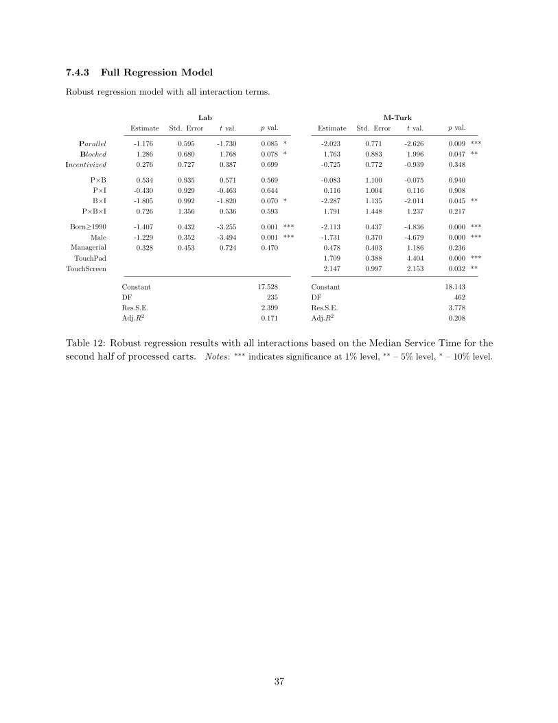
7.4.3 Full Regression Model
Robust regression model with all interaction terms.
Lab
Estimate Std. Error t val. p val.
Constant
DF
Res.S.E.
Adj.R2
17.528
235
2.399
0.171
Parallel *
Blocked *
Incentivized
-1.176
1.286
0.276
0.595
0.680
0.727
-1.730
1.768
0.387
0.085
0.078
0.699
P×B
P×I
B×I *
P×B×I
0.534
-0.430
-1.805
0.726
0.935
0.929
0.992
1.356
0.571
-0.463
-1.820
0.536
0.569
0.644
0.070
0.593
Born≥1990 ***
Male ***
Managerial
TouchPad
TouchScreen
-1.407
-1.229
0.328
0.432
0.352
0.453
-3.255
-3.494
0.724
0.001
0.001
0.470
M-Turk
Estimate Std. Error t val. p val.
Constant
DF
Res.S.E.
Adj.R2
18.143
462
3.778
0.208
***
**
-2.023
1.763
-0.725
0.771
0.883
0.772
-2.626
1.996
-0.939
0.009
0.047
0.348
**
-0.083
0.116
-2.287
1.791
1.100
1.004
1.135
1.448
-0.075
0.116
-2.014
1.237
0.940
0.908
0.045
0.217
***
***
***
**
-2.113
-1.731
0.478
1.709
2.147
0.437
0.370
0.403
0.388
0.997
-4.836
-4.679
1.186
4.404
2.153
0.000
0.000
0.236
0.000
0.032
Table 12: Robust regression results with all interactions based on the Median Service Time for the
second half of processed carts. Notes: ∗∗∗ indicates significance at 1% level, ∗∗ – 5% level, ∗ – 10% level.
37


![08 Queueing Models.ppt [Kompatibilitätsmodus] ... KeyelementsofqueueingsystemsKey elements of queueing systems ... • Customer is pendingwhen the customer is outside the queueing](https://img.pdfslide.us/doc/110x75/5b236bc17f8b9a92298b6c18/08-queueing-kompatibilitaetsmodus-keyelementsofqueueingsystemskey-elements.jpg)