Human Motion Capture Project

Jeff Marsh

Spring 2008

Contents

Introduction 1

Overview of the Motion Capture Format 2

Calculating Accelerations 3

Using the Matlab Routines 7

Acknowledgements 8

References 8

Appendix: Tables 10

Introduction

This article documents some of the work I’ve done processing motion captureinformation. It assumes the reader is already somewhat familiar with thesubject of motion capture, Acclaim file formats, and using Matlab.

Objective: Using motion capture data, obtain vector accelerations for thearms and legs of a human walking and running.

Motivation: The accelerations are to be used to enhance a mathematicalmodel of the human cardiopulmonary system (by Radu Cascaval, Uni-versity of Colorado).

1

Computer code: All code development was done using Matlab (version7.1.0.124 R14 service pack 3, but the routines should run on any morerecent version of Matlab).

Data: All the data come from the Carnegie Mellon University (CMU) mo-tion capture library [12]. I assume position data are in meters, timedata are in seconds, and the frame rate is 120 frames per second. I’venot tested these routines with any other data, but I see no reason theywould not work as long as the skeleton definition is the same.

File formats: I have worked exclusively with the Acclaim Motion Capture(AMC) and the Acclaim Skeleton File (ASF) formats [2, 6, 7, 11]. Theseare ordinary text files and the contents can be viewed and modified withany text editor.

Overview of the Motion Capture Format

This is a very brief overview of the Acclaim motion capture format andhow the data are processed; for details see the references below. Note thatthe skeleton description is specific to the CMU library; different skeletondefinitions are possible.

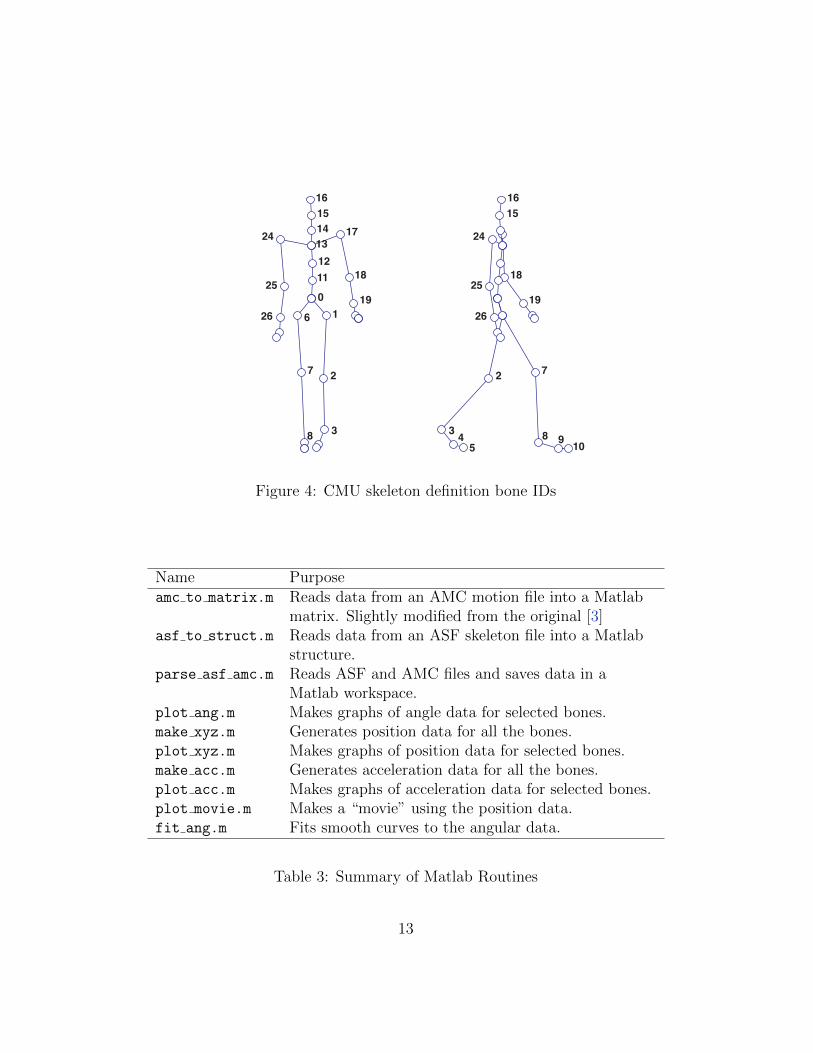
The skeleton file (ASF) defines a tree structure representing the humanskeleton. The edges of this tree represent rigid, fixed-length bones and thevertices represent joints. Each bone is assigned an ID number and a name,and with the exception of the root, has a unique parent. See table 1 andfigure 4.

The skeleton file defines the topology of the tree, the lengths of the bones,and the possible motions of each bone relative to its parent. Each subject inthe CMU library has a corresponding skeleton file.

The motion capture file (AMC) records the position of the bones at fixedintervals of time (I have assumed the frame rate is always 120 frames persecond). In each frame the position of the root vertex is recorded as Cartesiancoordinates in the world coordinate system. In addition, the orientation ofthe coordinate system attached to the root vertex is recorded as three Eulerangles. The position of each bone is then specified as three Euler anglesrelative to the parent bone’s coordinate system.

To determine the Cartesian coordinates of the endpoint of a bone inthe world coordinate system, one first determines the coordinates in the

2

parent bone’s coordinate system. This involves four operations: a translationfrom the parent bone’s origin, then three rotations, one for each Euler angle.Then one repeats this to obtain the coordinates in the grandparent bone’scoordinate system, then the great-grandparent bone’s system, and so on untilthe root bone is reached and ultimately we get the coordinates in the worldcoordinate system. Of course, all this is done for each bone and for eachframe. See [3–5, 10] for details.

The above procedure description is a bit of an oversimplification; theactual procedure isn’t too bad really, but figuring it all out was very diffi-cult. The major problem was that all the references I could find were eitherinsufficiently detailed or insufficiently precise. It took some guesswork andtrail-and-error to get it all to work.

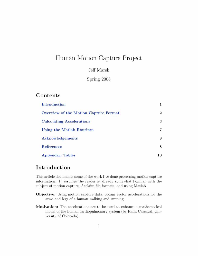
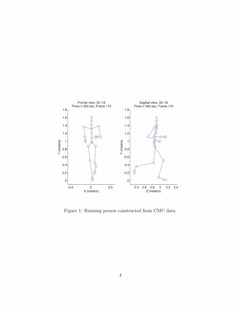
In all the files I have worked with, “up” is in the positive y direction andthe subject is moving in approximately the positive z direction.

The content of the skeleton file is summarized in table 1 and figure 4.An example of all this, as constructed from CMU data, is show in figure 1.

Calculating Accelerations

The accelerations may be approximated from the positions using the standardcentral finite-difference formula:

fi = (fi+1 − 2fi + fi−1) /h2

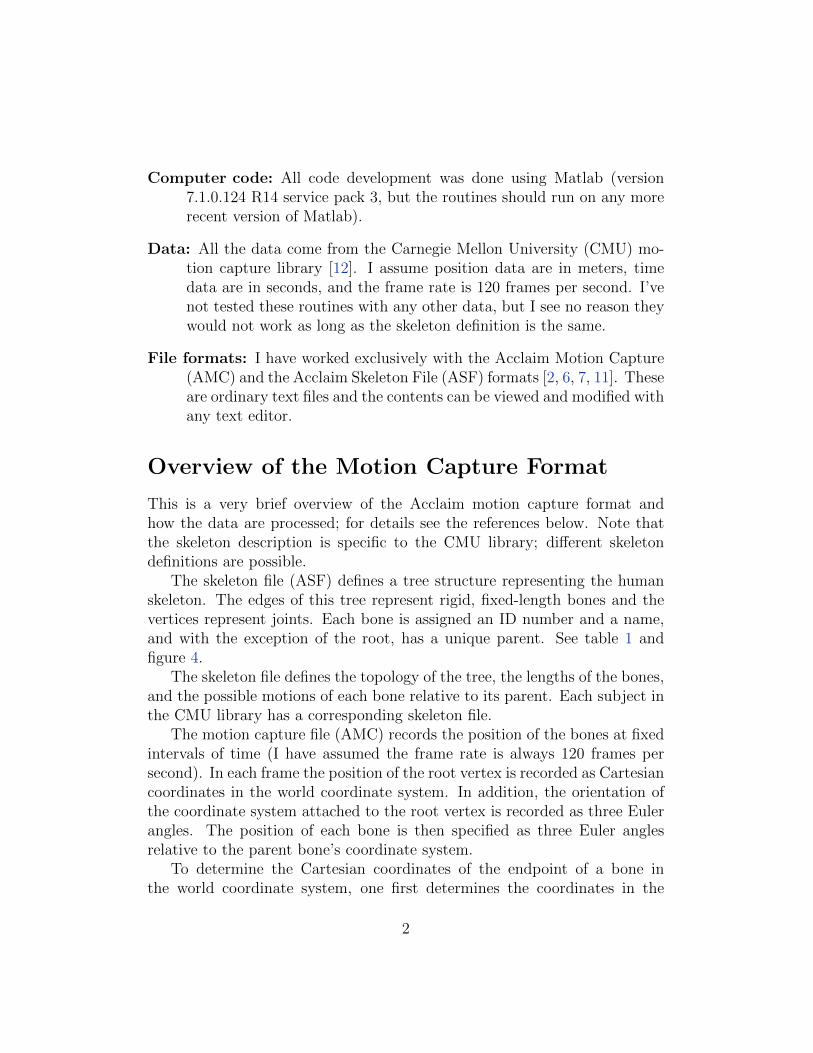
where h is the (assumed constant) time interval between samples, and thetruncation error is on the order of h2. Unfortunately, applying this for-mula directly to the x, y, z data produces garbage. This is because of theunavoidable presence of measurement noise in the original data. Since thesecond time derivative of any frequency component sin(ωt) is proportionalto ω2, high-frequency noise tends to be amplified in the computation of theacceleration. This can be seen in the following simple example.

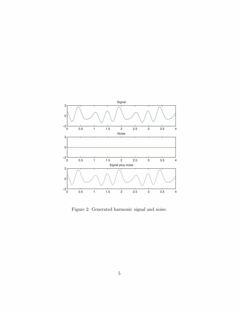
I’ve calculated a signal by summing several harmonic functions, as shownin the top graph of figure 2. I then generate some random noise (uniformlydistributed) equal to only 0.1 % of the signal (that is, the peak-to-peak noiseequals 0.1 % of the peak-to-peak signal). This noise is shown in the middlegraph of figure 2 — it is so small compared to the signal that it appears to

3

−0.5 0 0.5

0

0.2

0.4

0.6

0.8

1

1.2

1.4

1.6

1.8

X (meters)

Y (m

eter

s)

Frontal view, 35−18Time=1.450 sec, Frame 175

2.4 2.6 2.8 3 3.2 3.4

0

0.2

0.4

0.6

0.8

1

1.2

1.4

1.6

1.8

Z (meters)

Y (m

eter

s)

Sagittal view, 35−18Time=1.450 sec, Frame 175

Figure 1: Running person constructed from CMU data.

4

0 0.5 1 1.5 2 2.5 3 3.5 4−2

0

2Signal

0 0.5 1 1.5 2 2.5 3 3.5 4−2

0

2Noise

0 0.5 1 1.5 2 2.5 3 3.5 4−2

0

2Signal plus noise

Figure 2: Generated harmonic signal and noise.

5

0 0.5 1 1.5 2 2.5 3 3.5 4−400

−300

−200

−100

0

100

200

300

400

Blue: Exact accelerationRed: Acceleration calculated using finite differences

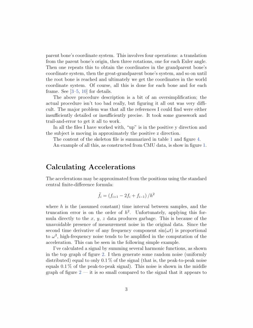
Figure 3: Calculated accelerations.

be a horizontal line. The signal plus noise is shown in the bottom graph offigure 2. At this scale, you can’t tell it from the original signal.

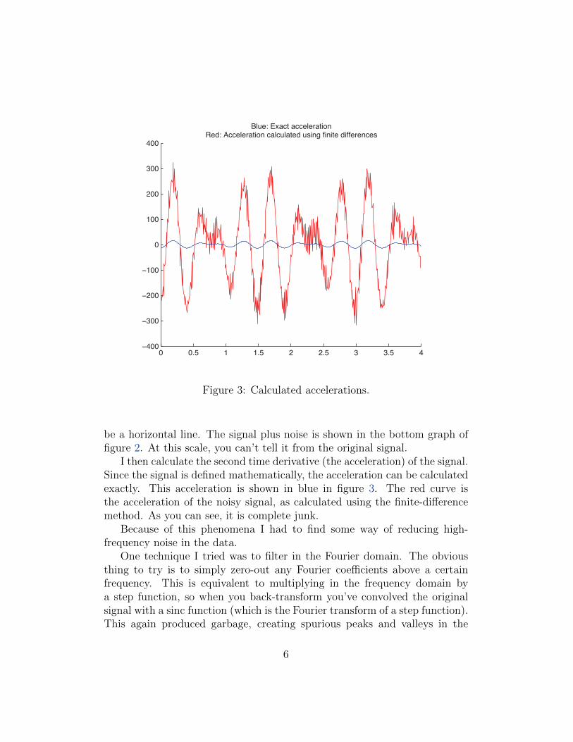
I then calculate the second time derivative (the acceleration) of the signal.Since the signal is defined mathematically, the acceleration can be calculatedexactly. This acceleration is shown in blue in figure 3. The red curve isthe acceleration of the noisy signal, as calculated using the finite-differencemethod. As you can see, it is complete junk.

Because of this phenomena I had to find some way of reducing high-frequency noise in the data.

One technique I tried was to filter in the Fourier domain. The obviousthing to try is to simply zero-out any Fourier coefficients above a certainfrequency. This is equivalent to multiplying in the frequency domain bya step function, so when you back-transform you’ve convolved the originalsignal with a sinc function (which is the Fourier transform of a step function).This again produced garbage, creating spurious peaks and valleys in the

6

original data. This sometimes made the subject look like he/she had thedelirium tremens.

Filtering in the frequency domain with a Gaussian was a little better.Since the transform of a Gaussian is another Gaussian, this has the effect ofconvolving with a Gaussian in the time domain. But this “Gaussian blur” hastwo undesirable side-effects: a local maximum (or minimum) gets reduced (orincreased) in the time domain, and the width of any peaks or valleys in thedata gets increased. I found that filtering sufficiently so that the accelerationsstarted to make sense would produce a “ghostly” motion, where the subjectjust drifts forward, barely moving, sometimes with his/her feet not eventouching the ground.

Another technique I tried is the Savitzky-Golay filter [9], which I selectedbecause it tends to preserve the width and heights of local maxima. Thisfilter computes a linear combination of data points within a moving win-dow; essentially a convolution in the time domain. This worked much betterthan the Fourier technique, but again, filtering sufficiently to get reasonableaccelerations produced unrealistic-looking motions.

I finally settled on simply fitting the raw angle data to a linear combi-nation of harmonic functions [13]. Ideally, for a subject walking and run-ning, each bone undergoes periodic motion. So I decided to model the time-dependence of a given Euler angle as:

c0 + c1 sin(ωt) + c2 cos(ωt) + c3 sin(2ωt) + c4 cos(2ωt) + . . .

where ω, c0, c1, c2, . . . are constants. For the x and z coordinates of the rootvertex, I add a linear term ct.

At this time I’ve not been able to get the routine to reliably converge whenestimating ω, so I require that the period of motion be estimated by handand input to the routine. However, all other constants are automaticallycalculated.

I was a little surprised at how well this works; only a few harmonics arenecessary to get a good fit to the data.

See [1] for more smoothing techniques.

Using the Matlab Routines

The routine parse asf amc.m prompts for the name of a skeleton file and amotion capture file, parses and copies the data into the workspace, and saves

7

the workspace. Once in the workspace, you can do anything you want to thedata. Use Matlab’s “load” command to load a saved workspace. Data fromthe skeleton file is put into the structure S (see table 2).

The data in the motion capture file is placed in the 2-dimensional matrixD. The first (row) index into D is the frame number, and the second (column)index into D gives the particular datum, see table 1 for a list. Most of thedata represent Euler angles (in degrees) specifying the position of the bone.Note that not all bones have all three degrees of freedom.

Important note: The plot routines simply plot whatever is in the currentworkspace. This is an advantage because the user can plot data from anysource, smoothed or un-smoothed, using the same routine. However, thedisadvantage is that it is the responsibility of the user to keep track of wherethe information came from and what has been done to it.

See table 3 for a summary of the routines.

Acknowledgements

The data used in this project were obtained from http://mocap.cs.cmu.

edu. This database was created with funding from NSF EIA-0196217.

References

[1] Allard, Stokes, and Blanchi, editors. Three-dimensional Analysis ofHuman Movement. Unknown publisher, 1995. See chapter 5,Smoothing and Differentiation Techniques Applied to 3D Data byHerman J. Woltring.

[2] Unknown Author. Acclaim ASF/AMC, 1999. URL http://www.cs.

wisc.edu/graphics/Courses/cs-838-1999/Jeff/ASF-AMC.html.Poorly written and consequently almost misleading; mixes the left andright multiplication conventions, and contains several typos. But doescontain some practical information on constructing the transformmatrices.

[3] Jernej Barbic. amc to matrix.m, 2003. URLhttp://graphics.cs.cmu.edu/software/amc_to_matrix.m. OriginalMatlab function.

8

[4] Jinxiang Chai. Motion Representation and Forward Kinematics, 2006.URL http:

//faculty.cs.tamu.edu/jchai/CPSC689/689_ppts/lecture2.ppt.Short on detail and contains some typos but it is a useful introductionto the subject.

[5] J. D. Foley and A. Van Dam. Fundamentals of Interactive ComputerGraphics. Addison-Wesley, 1982. Chapter 7 is a good introduction tohow the computer graphics people deal with matrices and transforms.

[6] Jeff Lander. Working with Motion Capture File Formats, 1998. URLhttp://www.darwin3d.com/gamedev/articles/col0198.pdf.Written for game developer wannabes, this is a fluff introduction to thefile formats; almost useless.

[7] M. Meredith and S. Maddock. Motion Capture File FormatsExplained, 2005. URL http:

//www.dcs.shef.ac.uk/intranet/research/resmes/CS0111.pdf.Does not specifically mention ASF/AMC file format, but containssome useful explanations of how to construct the transforms.

[8] NCHS. National Center for Health Statistics, 2008. URLhttp://www.cdc.gov/nchs/. A source for human body measurements.

[9] W. H. Press, S. A. Teukolsky, W. T. Vetterling, and B. P. Flannery.Numerical Recipes in C; The Art of Scientific Computing. CambridgeUniversity Press, 2nd edition, 1992. See section 14.8, Savitzky-GolaySmoothing Filters.

[10] Tido Roder. Similarity, Retrieval, and Classification of MotionCapture Data, 2006. URL http://hss.ulb.uni-bonn.de/diss_

online/math_nat_fak/2007/roeder_tido/. Detailed, comprehensive,and written for mathematicians. The appendix Representing rotationsof R3 is a real gem.

[11] M. Schafer. Acclaim File Definitions, 1994. URLhttp://www.darwin3d.com/gamedev/acclaim.zip. The zip filecontains two microsoft word documents: acclaimdef.doc, “AcclaimFormat - ASF line details”, and acclaimimp.doc, “Acclaim skeletonfile definition”. Terse, but useful.

9

[12] Carnegie Mellon University. Graphics Lab Motion Capture Database,2002. URL http://mocap.cs.cmu.edu/.

[13] Eric W. Weisstein. Nonlinear Least Squares Fitting, 2008. URL http:

//mathworld.wolfram.com/NonlinearLeastSquaresFitting.html.This details the procedure used to fit the angle data to harmonicfunctions.

Appendix: Tables

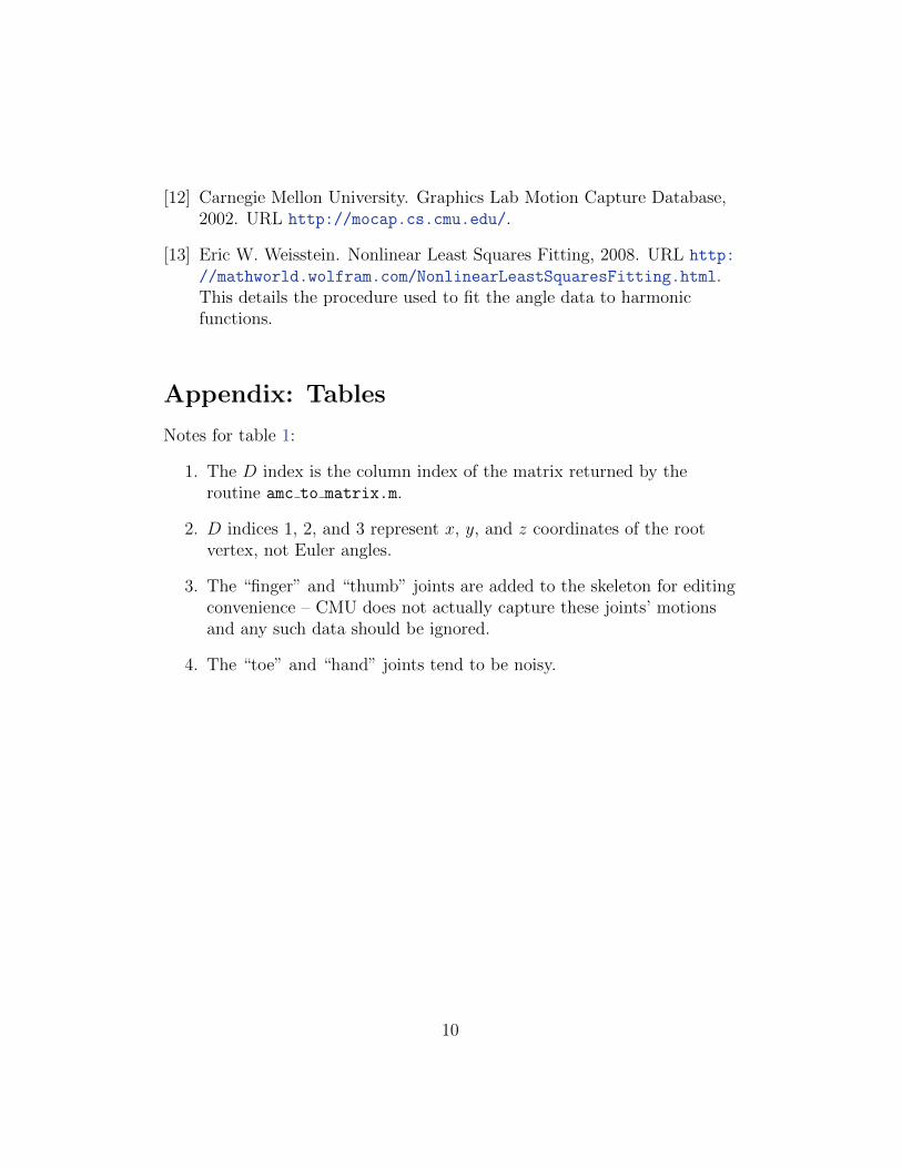
Notes for table 1:

1. The D index is the column index of the matrix returned by theroutine amc to matrix.m.

2. D indices 1, 2, and 3 represent x, y, and z coordinates of the rootvertex, not Euler angles.

3. The “finger” and “thumb” joints are added to the skeleton for editingconvenience – CMU does not actually capture these joints’ motionsand any such data should be ignored.

4. The “toe” and “hand” joints tend to be noisy.

10

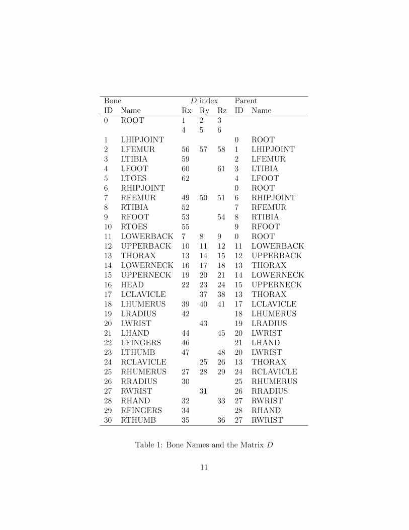
Bone D index ParentID Name Rx Ry Rz ID Name0 ROOT 1 2 3

4 5 61 LHIPJOINT 0 ROOT2 LFEMUR 56 57 58 1 LHIPJOINT3 LTIBIA 59 2 LFEMUR4 LFOOT 60 61 3 LTIBIA5 LTOES 62 4 LFOOT6 RHIPJOINT 0 ROOT7 RFEMUR 49 50 51 6 RHIPJOINT8 RTIBIA 52 7 RFEMUR9 RFOOT 53 54 8 RTIBIA10 RTOES 55 9 RFOOT11 LOWERBACK 7 8 9 0 ROOT12 UPPERBACK 10 11 12 11 LOWERBACK13 THORAX 13 14 15 12 UPPERBACK14 LOWERNECK 16 17 18 13 THORAX15 UPPERNECK 19 20 21 14 LOWERNECK16 HEAD 22 23 24 15 UPPERNECK17 LCLAVICLE 37 38 13 THORAX18 LHUMERUS 39 40 41 17 LCLAVICLE19 LRADIUS 42 18 LHUMERUS20 LWRIST 43 19 LRADIUS21 LHAND 44 45 20 LWRIST22 LFINGERS 46 21 LHAND23 LTHUMB 47 48 20 LWRIST24 RCLAVICLE 25 26 13 THORAX25 RHUMERUS 27 28 29 24 RCLAVICLE26 RRADIUS 30 25 RHUMERUS27 RWRIST 31 26 RRADIUS28 RHAND 32 33 27 RWRIST29 RFINGERS 34 28 RHAND30 RTHUMB 35 36 27 RWRIST

Table 1: Bone Names and the Matrix D

11

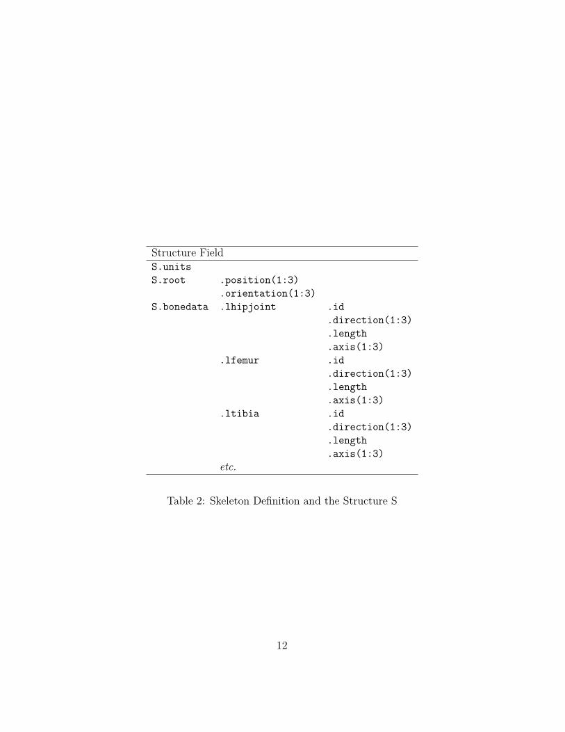
Structure FieldS.units

S.root .position(1:3)

.orientation(1:3)

S.bonedata .lhipjoint .id

.direction(1:3)

.length

.axis(1:3)

.lfemur .id

.direction(1:3)

.length

.axis(1:3)

.ltibia .id

.direction(1:3)

.length

.axis(1:3)

etc.

Table 2: Skeleton Definition and the Structure S

12

10

2

3

6

7

8

111213141516

17

18

19

24

25

26

3 45

2

8

7

9 10

1615

19

24

2518

26

Figure 4: CMU skeleton definition bone IDs

Name Purposeamc to matrix.m Reads data from an AMC motion file into a Matlab

matrix. Slightly modified from the original [3]asf to struct.m Reads data from an ASF skeleton file into a Matlab

structure.parse asf amc.m Reads ASF and AMC files and saves data in a

Matlab workspace.plot ang.m Makes graphs of angle data for selected bones.make xyz.m Generates position data for all the bones.plot xyz.m Makes graphs of position data for selected bones.make acc.m Generates acceleration data for all the bones.plot acc.m Makes graphs of acceleration data for selected bones.plot movie.m Makes a “movie” using the position data.fit ang.m Fits smooth curves to the angular data.

Table 3: Summary of Matlab Routines

13