Human Development Report 2006hdr.undp.org/sites/default/files/fuentes_et_al_a.pdfHuman Development Report 2006 ... urban/rural differences in the infant mortality rate ... estimation

Human Development Report 2006 Human Development Report Office OCCASIONAL PAPER

Does Access to Water and Sanitation Affect Child Survival? A Five Country Analysis Ricardo Fuentes, Tobias Pfütze and Papa Seck

2006/4

"Does Access to Water and Sanitation Affect Child Survival? A Five Country Analysis."

Ricardo Fuentes, Tobias Pfuetze & Papa Seck. This research was carried out as a background paper for Human Development Report 2006 “Beyond Scarcity: power, poverty and the global water crisis”. We would like to thank Partha Deb, Edilberto Loaiza, Howard White and Shea Rutstein for their helpful comments. We would also like to acknowledge the valuable insights provided to us by the members of the statistical advisory panel, Gareth Jones in particular, the entire Human Development Report Office team and finally this year’s advisory panel members. We have also benefited from excellent research assistance by Min Zang. The analysis and views expressed in this document do not necessarily reflect the views of the Human Development Report Office or the United Nations Development Programme. All remaining errors and omissions are solely the responsibility of the authors.

I) Introduction: About 10 million children die every year, most of them from preventable diseases. Although chance plays its role in this tragedy, poor living conditions are the main cause of this event. Children living in houses with poor ventilation, rustic floors and unsafe windows are more likely to suffer an accident, a disease or early death. Access to water and sanitation is a large element of the definition of decent, safe housing. Moreover, access to water and sanitation has large direct and indirect impacts on children's health: Many of the most pervasive diseases are water related1. The WHO estimates that water-related diseases account for 4% of all deaths and 5.7 % of the total disease burden (Pruss et all 2002). In this paper, we explore the linkages between types of water sources, sanitation facilities and mortality in the first year of life. For this, we use a set of household surveys -the Demographic and Health Surveys (DHS) conducted by Macro International. As the name indicates, the DHS collect and monitor population, health and nutrition indicators. The topic is of extreme relevance for human development. The place where a child is born will be determinant in her life and death. If she sees the first day of light in a household without running water and a toilet facility, she will be more likely to die from risks associated to poor environmental conditions. Previous research has found that the two most important factors explaining the decrease in under-five fatality during the 1990s were water supply, sanitation and improved nourishment conditions (Rutstein 2000). This paper is part of a two paper series. While it focuses on mortality, the companion paper addresses morbidity. Our main objective is to detect general patterns of the impact of water and sanitation conditions on neonatal and post-neonatal mortality; to this end we will present a broad series of estimations for different countries and regions. A word of caution is in place nonetheless when estimating the impact of different housing characteristics on mortality. Whether conditions of morbidity translate into deaths depend to a large degree on access and quality of health care among other things. We are not able to control for those factors. Our estimations represent therefore the combined effect of a variety of mechanism (behavioral, social, environmental) which we are not able to disentangle. In this context it is important to point out that our approach represents a social science approach as opposed to a medical science approach (see Mosely, Chen 1984). We determine the effect of A on B, without attempting to explain the precise chain of causation that leads there. To this effect, we use statistical methods extensively used in medical and economic research. To analyze the effect of household conditions on neo natal death we use a standard logit model where our variable to explain is the occurrence of death. To estimate the chances of survival in the next eleven months of life, we use a duration model, in particular a Proportional Cox Hazard model. 1 Among these are : cholera, typhoid, bacillary dysentery and gastroenteritis (water-borne) and scabies, trachoma, leprosy (water-washed) -Ashbolt 2004)

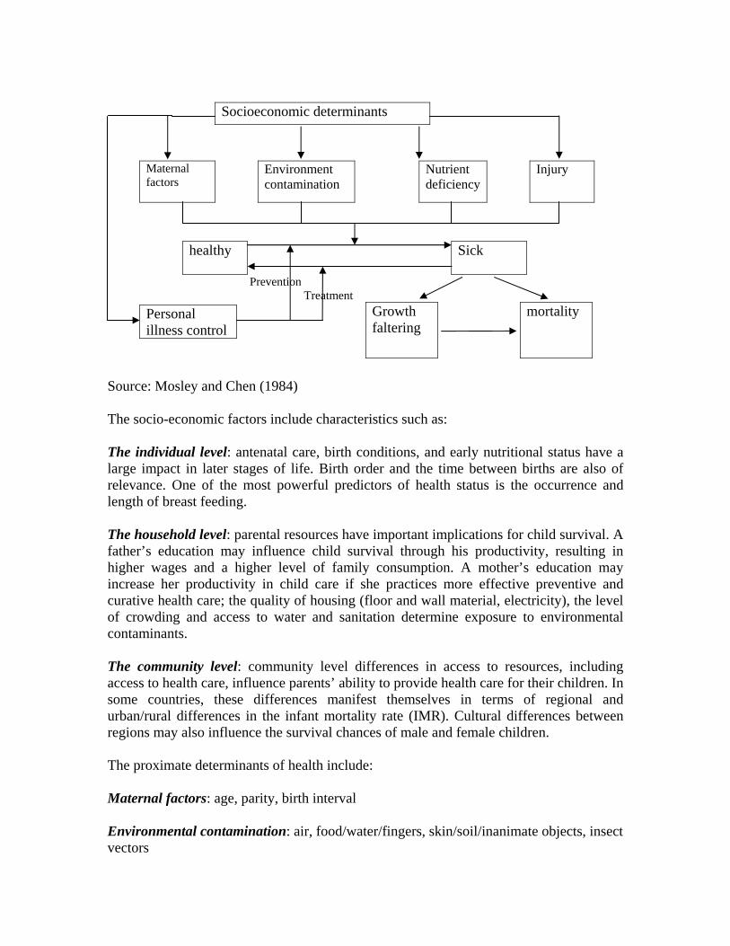
The paper is divided in six sections: section two provides a literature reviews, section three describes the data, section four discusses the methodology, section five shows the results obtained and the last section concludes. II) Framework and Literature Review : Framework There are two possible approaches to study the effects of water and sanitation –and household conditions in general- in the risk of premature death: the social science and the medical research methods. While the former tries to identify which socioeconomic variables have a significant impact on the odds of death at a young age, without trying to identify the biological processes underlying it, the latter focuses on precisely these processes without paying much attention to the underlying causes. Mosley and Chen (1984) propose a general theoretical model underlying each approach and a unifying framework which enables the integration of the two methods. This framework is the most comprehensive and systematic model for analyzing infant and child mortality. According to the Mosley-Chen framework, socio-economic factors at the community, household or individual level operate through proximate determinants of health to influence the level of infant and child mortality. The proximate determinants represent underlying mechanisms that influence the disease process. They include maternal fertility factors, environmental contamination, nutrient deficiency, injury and personal illness control, and are the pathway through which socio-economic processes affect infant health. The framework can be explained in a diagram:

Socioeconomic determinants

Maternal factors

Environment contamination

Nutrient deficiency

Injury

healthy Sick

Prevention Treatment

Growth faltering

mortality

Source: Mosley and Chen (1984) The socio-economic factors include characteristics such as: The individual level: antenatal care, birth conditions, and early nutritional status have a large impact in later stages of life. Birth order and the time between births are also of relevance. One of the most powerful predictors of health status is the occurrence and length of breast feeding. The household level: parental resources have important implications for child survival. A father’s education may influence child survival through his productivity, resulting in higher wages and a higher level of family consumption. A mother’s education may increase her productivity in child care if she practices more effective preventive and curative health care; the quality of housing (floor and wall material, electricity), the level of crowding and access to water and sanitation determine exposure to environmental contaminants. The community level: community level differences in access to resources, including access to health care, influence parents’ ability to provide health care for their children. In some countries, these differences manifest themselves in terms of regional and urban/rural differences in the infant mortality rate (IMR). Cultural differences between regions may also influence the survival chances of male and female children. The proximate determinants of health include: Maternal factors: age, parity, birth interval Environmental contamination: air, food/water/fingers, skin/soil/inanimate objects, insect vectors

Personal illness control

Nutrient deficiency: calories, protein, micronutrients (vitamins and minerals) Injury: accidental, intentional Personal illness control: personal preventive measures, medical treatment As explained in the introduction, our objective is to identify the likely impact of a policy relevant intervention, in particular the provision of adequate water and sanitation infrastructure. The exact biological means of transmission running from our variables of interest to mortality are of no direct interest in this study and are only taken into account as far as they might induce omitted variable bias. Literature Review Several empirical studies have used slight variations of this framework. A study conducted in the Brazilian state of Ceará (Terra de Souza et al 1999) using the 1991 census and the community Health Worker’s Program – a state government programme implemented in all but two of the 184 municipalities of Ceará- found that breastfeeding and ante natal care had a large correlation with infant mortality rates, defined as the ratio of infant deaths to live births in the 30 month duration of the study. However, no association could be established between sanitation facilities and mortality rates, mainly because the data did not present enough dispersion – sanitation is uniformly of bad quality across municipalities of Ceará. A similar study conducted in Egypt (Abou-ali Hala 2003) found a strong and negative relationship between the quality of the water source, sanitation facilities and mortality rates after the first month of life. This study used information from the 1995 Demographic and Health Survey and applied several methodologies including parametric and non-parametric duration models. This study draws heavily on previous similar studies in Eritrea and Sri Lanka. A third study conducted in Ghana (Asenso-Okyere et al 1997) attempted to gauge the determinants of nutritional and health conditions for children using the Ghana Living Standards Measurement Survey. The results show that breastfeeding and education of the mother present the largest impact in the nutritional status of children. The authors also suggest as part of their policy recommendations to improve water and sanitation conditions. Several other studies have used micro data to capture the determinants of children health, tough not necessarily using the Mosley-Chen Framework. The advent of standardized household surveys such as the Demographic and Health surveys and the Multiple Indicator Cluster Surveys have made this strand of research more feasible. Research in Pakistan (Agha 2000), sub-Saharan Africa (Madise et al 1990) and Central America and the Caribbean (Hojman 1996) among many have shown the importance of mother’s education and breastfeeding in health status.

In our study, we attempt to detect general patterns of how access to clean water and sanitary facilities affect mortality risk during the first year of life across countries. To this end we conduct our estimations for five countries: Cameroon, Egypt, Peru, Uganda and Viet Nam. We surveyed several of the studies cited above to identify the common characteristics that affect the chance of surviving in urban and rural areas. Moreover, we also test the consistency of our results using Propensity Score Matching for most of our initial estimations. III) Estimation methods: Logit and Proportional Hazard The risk of mortality in the first year of life can be decomposed into two different statistics. The first is neonatal mortality, which we define here as death within the first month of life, the second is post-neonatal mortality, understood as death after the completion of the first month of life but before the completion of the first year. We decided to partition the analysis this way because the elements affecting the health status and chances of survival for newborn children are very different from those elements that can have an impact for infants. Our survey data reports whether a child died within the first five years of life and the age at death in months. The estimation strategy for neonatal mortality is straightforward: We use a standard logit estimation where our dependent variable equals one if a child dies within the first month of life and zero otherwise. Our control variables consist of a set of dummy variables which are explained in the next section. To capture the determinants of post-neonatal mortality we use a more elaborate estimation method given the presence of censored observations. Children in our sample can drop out due to death or because they haven’t completed the first year of life at the time of the interview. In other words, the data used do not contain observations for the entire period of analysis for all children. For example, a child who is four months old at the time of the interview and dies at age five months will not be recorded in the survey as a death. This child will be considered a survivor when in reality he will not reach the first year of life. One way to address this problem would be to restrict our sample to those children who were at least one year old at the time of the interview; however this could create sample selection problems and eliminate a considerable number of observations. We choose instead to use a hazard model which accounts for issues of censoring (see Greene, 2000, chapter 20, for an exhaustive discussion of hazard models). We follow an extensive literature on mortality and apply a Cox Proportional Hazard Model (Cox, 1972) which is a semi-parametric estimation given that the underlying hazard rate is not modeled by some functional form. This model has only one requisite structural assumption; the effect of the covariates on the relative hazard rate must be constant over the time period under consideration.

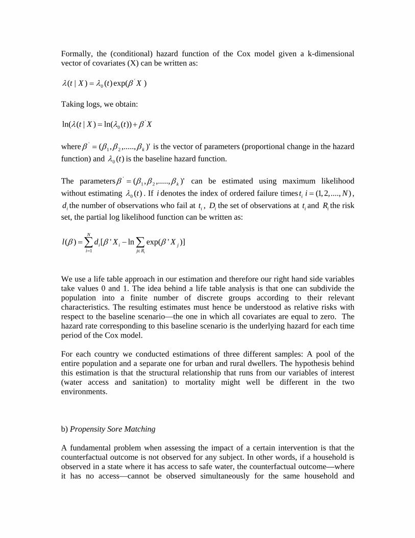
Formally, the (conditional) hazard function of the Cox model given a k-dimensional vector of covariates (X) can be written as:

XtXt '0 exp()()|( βλλ = )

Taking logs, we obtain:

XtXt '0 ))(ln()|(ln( βλλ +=

where )',.....,,( 21

'kββββ = is the vector of parameters (proportional change in the hazard

function) and )(0 tλ is the baseline hazard function. The parameters )',.....,,( 21

'kββββ = can be estimated using maximum likelihood

without estimating )(0 tλ . If i denotes the index of ordered failure times it (1,2,...., )i N= ,

id the number of observations who fail at it , iD the set of observations at it and iR the risk set, the partial log likelihood function can be written as:

1( ) [ ' ln exp( ' )]

i

N

i i ji j R

l d X Xβ β β= ∈

= −∑ ∑

We use a life table approach in our estimation and therefore our right hand side variables take values 0 and 1. The idea behind a life table analysis is that one can subdivide the population into a finite number of discrete groups according to their relevant characteristics. The resulting estimates must hence be understood as relative risks with respect to the baseline scenario—the one in which all covariates are equal to zero. The hazard rate corresponding to this baseline scenario is the underlying hazard for each time period of the Cox model. For each country we conducted estimations of three different samples: A pool of the entire population and a separate one for urban and rural dwellers. The hypothesis behind this estimation is that the structural relationship that runs from our variables of interest (water access and sanitation) to mortality might well be different in the two environments. b) Propensity Sore Matching A fundamental problem when assessing the impact of a certain intervention is that the counterfactual outcome is not observed for any subject. In other words, if a household is observed in a state where it has access to safe water, the counterfactual outcome—where it has no access—cannot be observed simultaneously for the same household and

essentially becomes a missing data problem. Specifically, there might be an unobserved characteristic that drives both the quality of the water source and the occurrence of death. If this would be the case, the result from the logit and proportional hazard model would be biased. Evaluation studies seek to remedy this problem by estimating an average treatment effect (ATE), which amounts to comparing the mean outcome for the treated (Y=1) to that of untreated group (Y=0). The estimation of the conditional mean outcomes using any probability model will give consistent estimates of the true effect only if program placement (having access to safe water and toilet facilities in our case) is exogenous. For example, in the program evaluation framework, people can chose or decline to participate in a specific program (self selection). Due to this self selection, the error term in the regression will not vanish in expectation, introducing a source of selection bias. Due to this violation of the exogeneity of placement, the conditional mean outcome will be a biased estimate of the true effect. This topic is discussed at length in Ravallion (2005). The gold standard in this kind of study is what is generally referred to as experimental design where subjects are randomly placed in one of two groups (some assigned the treatment and some used as a control group) essentially guaranteeing the conditional mean independence. In the absence of an experiment, as is generally the case, one has to worry about unobserved characteristics that may be correlated with the treatment variable or expressed differently, cov( , ) 0i iD ε ≠ where

iD is treatment characteristic and iε is the error term. In our case, it may well be that some parents care more about the welfare of their children than others (which can be correlated with the type of water children will be given), something that is inherently unobserved, but will potentially affect the child’s survival status. Instrumental variable regression can remedy the problem, but the search for a valid instrument is not always a straightforward exercise, especially given the pervasive natures of neonatal and post-neonatal mortality. Propensity Score Matching methods (PSM) attempt to circumvent the counterfactual problem by essentially creating an observational analogue of the natural experiment. In PSM, subjects are matched on a vector of pre-treatment characteristics (Zi) using the probability of treatment ( )iP Z . Rosenbaum and Rubin (1983) show that if treatment is independent across subjects and outcome is independent of participation given Xi, then outcome is also independent of ( )iP Z . Intuitively, if households are matched on pre-treatment characteristics, it is as if they were selected randomly, one assigned to the treatment group and the other representing the counterfactual. Once these conditions are met, PSM will consistently estimate the ATE. There are essentially three steps to propensity score matching. First, the probability of participation is estimated as:

)'()1Pr( ii ZD βΦ== where (.)Φ is the normal distribution, iZ is a vector of pre-treatment characteristics and iD is the treatment variable. The resulting predicted probabilities represent the propensity score for each household. In the next step, households are sub-classified into propensity score strata using the score of households that fall in the region of overlap between treated and control groups using nearest neighbor matching (five nearest neighbors in our case). To avoid using the same unit several times, the treatment group needs to be smaller the control group. Using five strata generally removes 90% of the pre-treatment bias (Caliendo and Kopeinig, 2005). Within each stratum, a group means test is performed to check the balancing properties between treated and non-treated groups. Higher order terms and interactions are added as needed for the unbalanced covariates and the process is repeated until the balancing properties are satisfied. In the last step, one can perform a group means test for the outcome of interest or multivariate regression on the matched sample. If after matching some variables fail to satisfy the balancing property, they can be added as additional controls in a regression. IV) Data: Demographic and Health Surveys We use Demographic and Health Surveys (DHS), the most extensive standardized dataset on housing and demographic characteristics. The DHS are mostly funded by USAID within its “Monitoring and Evaluation to Assess and Use Results” (MEASURE) program. These surveys collect information on a wide set of variables at the individual, household and community level and are conducted every five years to allow comparisons over time. They usually sample 5,000-30,000 households in each round but don’t have a longitudinal design. Neonatal and post-neonatal deaths, even though they are tragic, constitute a rare event in statistical terminology. This poses a well known problem when estimating binary dependent variable models such as ours. The resulting estimators are consistent but downwardly biased. They also tend to underestimate the significance of a certain covariate. The rate at which this bias goes asymptotically towards zero is a function of the frequency with which a “success” event occurs (in our case a death) and the sample size. King and Zeng (2001) show that for estimations using a logistical model, this bias can be sizable if “success” events are rare (less than 3% of all observations) even though sample sizes are fairly large. Their paper also provides a good treatment of the general problem. This has several implications for our work: the estimates obtained during this research, are likely to be underestimates of the real impact. The problem is of course exacerbated when we estimate two separate models for the urban and rural population in each

country. Below we will provide further information on sample size and death rates for the five countries for which we carried the analysis. We present two approaches to partially mitigate this problem. For countries where the sample size or mortality incidence were too small in the latest DHS available, we follow the same strategy as in World Bank (2005) and merge the data with the survey from the preceding round. This procedure is admissible under the assumption that the structural relationship between our variables of interest and mortality are stable over time. We can do this since the households included are randomly sampled in each survey round An obvious implication of these problems outlined above is that one has to worry about unobserved characteristics that could bias the estimates. As a consistency check, we use the propensity score estimation methods explained in the previous section for the neonatal mortality exercise. A final implication of the rare event problem is that it forces us to specify a model as parsimonious as possible, since our estimates would be quickly rendered insignificant due to degree of freedom considerations. This is especially a concern with respect to the inclusion of interaction terms between water and sanitation variables since the number of control variables rapidly explodes. Another caveat in the exercise arises from the fact that the number of deaths occurred over the five year period prior to the interview while our covariates correspond to the moment of the interview. This is however another instance in which the true effect is most likely going to be underestimated. The reasoning is that, absent such tragedies as war or major natural disasters, a household is likely to improve its living conditions over time, especially since both latrines and water supply infrastructures are considered to be durable goods. We would therefore match, on average, more deaths with improved living conditions than with deteriorated ones which would lower our estimate for the impact of our variables of interest. It is also likely to add to the variance in the data and hence to lower p-values. Variables included For the purpose of our analysis, we use children as the primary subjects. We attempt to identify the elements that impact the chances of survival in different stages of life. First, we estimate the effects of individual, household and community characteristics which contribute to neonatal mortality. For this purpose, we define our main variable as a discrete indicator with two values: 0 if the child is alive and 1 if the child died during the first month of life. To estimate the impact of different elements into post neonatal survival, we define the outcome as a discrete time variable ranging from 1 to11 indicating the occurrence of

death between the second and the eleventh month of life. We proceed by using a Cox proportional hazard model to estimate the chances of survival. We included a set of control variables that can be categorized in three distinct groups following the Chen-Mosley framework: individual, household and community indicators. Individual level control variables: education of the mother, age of the mother at birth of child, length of birth interval, sex of child, access to media, whether the child was ever breastfed, mother’s knowledge of oral re-hydration therapy (ORT). Household level control variables: access to electricity, type of floor in dwelling, type of water facility, type of sanitation facility, religion of the mother and wealth status. It is worth expanding on this last variable. Since the main interest of our study is to capture the effect of water and sanitation infrastructure on health outcomes, we had to construct our own wealth index that would exclude these variables. We followed the standard procedure for the construction of wealth indices as indicated in World Bank 2005. We included eight different household assets to calculate the first principal component, with this information we constructed a standardized index using principal component analysis. Households were then subdivided into quintiles based on their asset score. Community level controls: urban/rural, and season of birth A brief explanation of the variables related to water and sanitation will clarify the terms used in the study. In the estimations of the models we used the definitions that are explained below: Safe Water: We followed the Joint Monitoring Program (JMP) definition of improved water with the exception of rain water. It corresponds to a household having access to piped water or a covered well. Independent Water: Indicates whether a household has access to a private water source or whether more than one household share a single water supply. Flush Toilet: Indicates whether a household has a flush toilet. Pit Toilet: Indicates whether a household has a pit latrine. Improved Toilet: Indicates whether a household has a flush toilet or an improved pit latrine. Traditional Toilet: Indicates whether a household has an unimproved/traditional pit latrine. This term is generally used in contrast to Improved Toilet, while the pair Improved/Traditional Toilet is used interchangeably with the pair Flush/Pit Toilet.

Toilet Facility: Indicates whether a household has any toilet facility at all. This term is used when not enough observations are available to distinguish between toilet types. All the control variables were codified as dummy indicators, in other words, all independent variables take values either 0 or 1. This allows for an easier interpretation of parameters. It is important to note that not all variables are available for all countries and that in some cases a particular control is not included due to lack of dispersion in that indicator. Our control variables are generated in such a way that our baseline corresponds to a worst case scenario. The characteristics of the sample under study are presented on table 2. Countries in Sub-Saharan Africa (Cameroon and Uganda) display the highest rates of mortality, 9.9% and 10.3% of children do not live past their first birthday in Cameroon and Uganda respectively. The corresponding figures are 5.6% for Egypt, 4.6% for Peru and a relatively low 2% for Vietnam. Access to a safe water source is high in Egypt (90.2%), compared to less than 60% for Peru, Uganda and Cameroon and 67.6% for Vietnam. Access to a toilet facility paints a more sobering picture. In Uganda and Cameroon respectively, 98.1% and 95% of children live in a household without access to a flush toilet. For Peru, more than a third of children live in a household without access to a toilet facility. The corresponding figures are 26% for Vietnam and 15% for Egypt. The sex ratio (girls for 100 boys) is close to one for all countries except in Vietnam where there are almost 105 boys for every 100 girls. An educated mother is a desirable feature but countries display wide disparities on that indicator. Egypt displays the lowest proportion of children with educated mothers; only 45% of children in the Egyptian sample have a mother with some form of formal education. In Cameroon and Uganda, a quarter of the children have uneducated mothers. This is in contrast with Vietnam and Peru where respectively 90.2% and 89.5% of children have educated mothers. As expected, breastfeeding is a widespread practice in all of the countries, with Egypt being the only exception at 64%. The knowledge of Oral Rehydration Therapy (ORT) is more mixed with high levels recorded in Egypt and Uganda. Overall, more than half of the children in the surveys live in rural areas, with disproportionately high levels found in Vietnam and Uganda (respectively 80% and 76%). Table 3 shows the distribution of access to safe water stratified by wealth quintile. Access to a safe water source seems to be wealth dependant. At the bottom of the wealth distribution, a greater proportion of children do not have access to a safe source of water supply. This picture is reversed at the top of the income distribution. These differences are especially stark in Peru where 66% of children in the poorest quintile do not have access to safe water, compared to 5.4% of those in the richest quintile. The comparative figures are 58% and 8% for Vietnam, also an indication of high levels of inequality. This

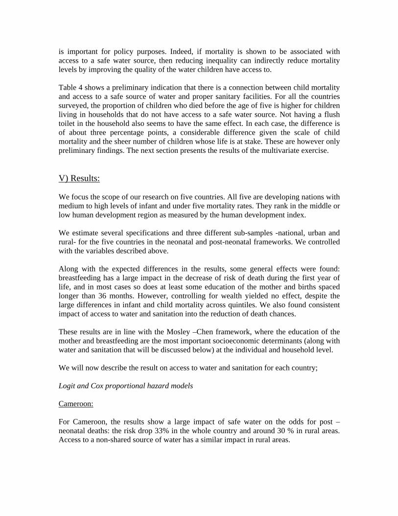
is important for policy purposes. Indeed, if mortality is shown to be associated with access to a safe water source, then reducing inequality can indirectly reduce mortality levels by improving the quality of the water children have access to. Table 4 shows a preliminary indication that there is a connection between child mortality and access to a safe source of water and proper sanitary facilities. For all the countries surveyed, the proportion of children who died before the age of five is higher for children living in households that do not have access to a safe water source. Not having a flush toilet in the household also seems to have the same effect. In each case, the difference is of about three percentage points, a considerable difference given the scale of child mortality and the sheer number of children whose life is at stake. These are however only preliminary findings. The next section presents the results of the multivariate exercise. V) Results: We focus the scope of our research on five countries. All five are developing nations with medium to high levels of infant and under five mortality rates. They rank in the middle or low human development region as measured by the human development index. We estimate several specifications and three different sub-samples -national, urban and rural- for the five countries in the neonatal and post-neonatal frameworks. We controlled with the variables described above. Along with the expected differences in the results, some general effects were found: breastfeeding has a large impact in the decrease of risk of death during the first year of life, and in most cases so does at least some education of the mother and births spaced longer than 36 months. However, controlling for wealth yielded no effect, despite the large differences in infant and child mortality across quintiles. We also found consistent impact of access to water and sanitation into the reduction of death chances. These results are in line with the Mosley –Chen framework, where the education of the mother and breastfeeding are the most important socioeconomic determinants (along with water and sanitation that will be discussed below) at the individual and household level. We will now describe the result on access to water and sanitation for each country; Logit and Cox proportional hazard models Cameroon: For Cameroon, the results show a large impact of safe water on the odds for post –neonatal deaths: the risk drop 33% in the whole country and around 30 % in rural areas. Access to a non-shared source of water has a similar impact in rural areas.

In terms of sanitation, the results in urban places show that access to an improved toilet reduces the risk of death by around 40 %, although in this case water does not seemingly have any effect on the chances of surviving. This leads to some conjectures that might deserve further exploration: namely that the quality of water is of extreme importance in rural areas, both the ownership structure and the type of infrastructure, while in cities a small improvement in the sanitation facilities can provide a large health safeguard. When we conduct the analysis on neo natal deaths, we found that children living in household with shared sources of water have a 60 % higher risk of dying in the first month of life. The result is particularly strong in rural areas although it is close to reach statistical significance when we run the estimation for the whole country. Egypt: In the case of Egypt we pooled the two most recent surveys (we include a control variable for the survey year), and have as our only wealth proxy whether a household has electricity2. We furthermore distinguish between traditional flush toilets and modern ones, while pit latrines are merged into the baseline scenario. The results are very strong. For neonatal mortality we find that safe water is significant and has a strong impact on the chances of survival – 35 % in the whole country and around 75 % in urban areas. A non-shared water source can also reduce the probability of early death: in urban areas the effect can reach about 60 % decrease in the risk of neonatal decease. Sanitation is not consistently significant under any specification. However, some of the estimations suggest that having access to a modern toilet facility can somewhat reduce the risk of death. In both the national and rural specification, access to a safe source of water reduces the probability of early death by 30%, while access to a modern toilet cuts this same risk by more than half. The results also show that the relative improvements of sanitation facilities have, as we expected, on the chances of surviving: while going from no sanitation facility to a traditional toilet reduces the risk of fatality by 25 %, the impact of a modern toilet is much larger, around 55%, as mentioned above. In urban areas of Egypt, sanitation has an even larger impact: the hazard rates decline by two thirds with the presence of a traditional toilet and by around 80% with a modern one. As in the case of Cameroon, the results suggest that the main infrastructure element in urban areas is sanitation while water plays a larger role in rural settings.

2 Due to the lack of enough socio-economic indicators, we were not able to calculate a wealth index for Egypt.

Peru: As in the case of Egypt, we pooled the two most recent surveys to expand our sample size. Our results showed an important impact on mortality through sanitation improvements. In the case of neonatal deaths having a pit latrine reduces the risk by about 27% in the whole country, while having access to a flush toilet does so by about 40%. It appears reasonable to say that the latter result is driven by the urban sector, where a flush toilet reduces the risk by more than 60% while in the rural areas the result does not hold in statistical terms. The existence of a pit latrine results in a 55% reduction in the odds of premature death. In particular, using the post neonatal sample for the whole country, we found that access to a flush toilet reduces the hazard rate significantly - by around 40%. In the urban sector the improvement in the chances of survival is larger, by about 70%; having access to a pit latrine also increases the chances avoiding early death by 50%. Uganda:

For Uganda we found strong evidence that both interventions, improvements in water and sanitation, have a significant effect on mortality decline. A safe water source lowers the risk rate by 22% when we analyzed the whole country. When we focused our attention only on rural areas, we obtained a very similar result – a reduction of 23 %. In the case of sanitation, we estimated the effect of having a pit latrine on the chances of child survival at 40% for the whole country and 40 % for the rural areas. Vietnam: With Vietnam, the issue of small sample size is more acute; the sample size for these surveys (we merged the two most recent surveys in this case as well) is less than 3,000 observations. As a result we were not able to estimate a separate model for the urban areas. However the results are very strong and were tested in several ways to check their stability. The only variables which turned out to be consistently significant are water related when analyzing post neonatal death. The impact is very strong and very similar in size for both accesses to safe water and access to a non-shared water source –around 78 % reduction in risk. When we focus our attention to neo natal mortality, we found sanitation infrastructure to be the driving force behind risk of early death decrease: our results show that going from the scenario with no sanitation facility to having access to a pit latrine reduces the chances of decease by 60 %, while a further improvement to a flush toilet reduces the

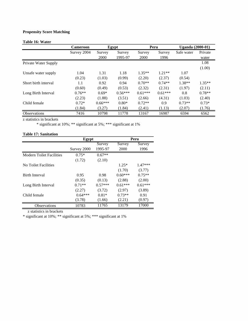
same risk by an additional 16 %. The results hold when we change the definition of sanitation facility: we compare a baseline scenario with no access to any sanitation facility to a scenario where children have access to traditional facilities, with an associated reduction in risk of 55 %, and to a situation with access to an improved facility (with a 83 % drop in the chances of death). Propensity Score Matching As the discussion above indicates, PSM is a labor intensive process. In order to avoid matching samples from different years, the steps described above were performed for each survey separately (a total of six surveys for access to water) and four surveys for sanitation. For Uganda, the same exercise was also repeated for access to a private water supply. Due to space constraints, the results of the test of the balancing properties for the various surveys are not presented. For each survey, we compared the percentage difference in means before matching to the difference after matching and also the model’s predictive power before and after matching. For all the surveys, we had low recorded R2 after matching which indicate that the matching variables had no remaining predictive power and do not explain the model anymore. In other words, the matched households are similar on all of these characteristics. Once the balancing properties were satisfied, we proceeded by estimating logistic regressions of neonatal mortality on access to water and sanitation separately. For variables with substantial remaining bias (over 5%), a regression adjustment method in which the variables are included as controls was used. The results are presented on tables 16 and 17. The results are as expected. Having an unsafe water supply increases the odds of dying by 35% and 21% in Peru (columns 4 and 5). For all the other surveys, the results point in the same direction but the odds are not significant. The relationship is clearer once we move to sanitation. Having modern toilet facilities in Egypt (the 2000 and 1996-97 surveys respectively) is associated with a 25% and a 33% decline in the probability of death, while for Peru, the absence of toilet facilities increases the chance of dying by 25% and 47% respectively. At first there seems to be a peculiarity in these results. New born babies after all are not directly affected by the water and sanitation infrastructures. Nevertheless, it is not implausible that they are indirectly affected, through bottled milk perhaps in the case of water and their interaction with other members of the household for sure in terms of sanitation. This latter channel can certainly constitute the deadly link between the increased risk of neonatal fatality and the lack of proper sanitary facilities. Other channels are also likely such as contamination and so on. This suggests that combining proper sanitary facilities and other hygienic practices can help reduce death rates for newborns. As stated earlier however, the purpose of this study is not to catalogue and investigate the different channels separately.

Another result worth mentioning is that girls have a much higher chance of survival than boys in virtually all of these countries. This is an indication that greater attention should be paid to girls in the first stages of life as this could affect gender ratios upstream. VI) Conclusions: The results outlined above show some clear trends: the seemingly consistent finding that access to safe water is more important in rural areas and access to an improved sanitation facility can increase the chances of survival in cities; we did not find strong consistent evidence of the impact of water and sanitation in neo natal deaths –although this is in line with what the literature suggest: neonatal deaths are determined by ante natal care and mothers health status and overall household sanitary behavior, while later diseases are more influenced by conditions in the household and the community. We also found some evidence that having access to a non shared water source or a private toilet can have a positive impact in the survival chances of children. Although these results were not significant across countries, the recurrence suggests that a “tragedy of the commons” might be present in some parts of the countries at study: lack of clear accountability might lead to pollution of the water source and thus to a higher risk of early death. In addition, the fact that water has to be transported for relatively long distances could very well be another potent source of contamination. The size of the reduction is very relevant: in every case where we found the effect to be significant, it is larger than 30%. Unfortunately, we could not test for the complementarities between both interventions under the current setting (the interactions were not significant when included in the specification, mostly due to the lack of variation in the data) although some of the results vaguely suggest a strong degree of complementarities between the two. Another interesting finding shows that the gradual improvements in the quality of infrastructure have a distinctive effect: as it was expected, the risk of death is reduced when a child has access to a pit latrine when compared to not having access to any type of sanitation, but the reduction is larger when the household has a flush toilet. This result also holds for the quality of water sources. As expected, one of the most consistent finding in the study is the importance of mother’s education and knowledge. Higher levels of schooling of the mother, knowledge of oral re-hydration therapy and breastfeeding practices are strongly associated with lower chances of disease. Unfortunately, we could not test for the linkages between mother’s education, use of water and sanitation infrastructure and fewer deaths. It is expected that the mother’s level of education influence the behavior of all members of the household, in particular in terms of hygiene. Further analysis on this issue is needed.

When testing the consistency of our result using propensity score matching, we found that the results hold, especially in the case of sanitation. There are several policy recommendations that emerge from this study: the quality of water and sanitation is very important, and constant improvements will reduce the chances of child death by a significant percentage. However, community arrangements, such as clear mechanism to share and maintain water sources, can also have an important role in risk reduction. The effect of other control variables suggests that education and knowledge of preventive measures play an important role in child survival, even more than asset ownership. Thus, an optimal policy would mix improvements in infrastructure, in community mechanism to maintain the water and sanitation facilities and programs to educate members of the household, in particular the mother, on how to make a better use of those facilities.

References Abou-ali, Hala. 2003 “The effect of water and sanitation on child mortality in Egypt,” Working paper in economics provided by Department of Economics, Goteborg University. Agha, Sohail. 2000. “The determinants of infant mortality in Pakistan,” Social Science & Medicine 51: 199-208. Asenso-Okyere, W.K., F.A. Asante, M. Nube. 1997. “Understanding the health and nutritional status of children in Ghana,” Agricultural Economics 17: 59-74. Bartlett, Sheridan. 2005. “Water, Sanitation and Urban Children: the Need to Go Beyond “Improved” Provision,” Children, Youth and Environments 15(1): 115-137 Caliendo, Marco and Sabine kopeinig. May 2005. “Some practical guidance for the implementation of propensity score matching”. IZA discussion paper No 1588. http://repec.iza.org/dp1588.pdf Deaton, Augus. 2003. “Health, inequality, and economic development,” Journal of Economic Literature, vol. XLI (March) pp: 113-158. Haines, Michael R., and Roger C. Avery. 1982. “Differential infant and child mortality in Costa Rica: 1968-1973,” Population Studies, vol. 36, no.1 (Mar.): 31-43. Hojman, David E.. 1996. “Economic and other determinants of infant and child mortality in small developing countries: the case of Central American and the Caribbean,” Applied Economics 28: 281-290 Julie Da Vanzo, W.P. Butz, and J.-P.Habicht. 1983. “How biological and behavioral influences on mortality in Malaysia vary during the first year of life,” Population Studies, vol. 37, no. 3 (Nov.): 381-402. Larsen B. 2003. “Hygiene and health in developing countries: defining priorities through cost - benefit assessments,” International Journal of Environmental Health Research 13 Suppl 1:S37-46. Lee, Lung-fei, Mark.R. Rosenzweig, and Mark.M. Pitt. 1997. “The effects of improved nutrition, sanitation, and water quality on child health in high-mortality populations,” Journal of Economics 77: 209-235. Leuven Edwin and Barbara Sianesi. 2003. “psmatch2: Stata’s module to perform full Mahalanobis and propensity score matching, common support graphing, and covariate imbalance testing”. http://ideas.repec.org/c/boc/bocode/s432001.html

Madise. Nyovani J., Zoe Matthews and Barrie Margetts. 1990. “Heterogeneity of child nutritional status between households: a comparison of six sub-Saharan African countries,” Population Studies 53: 331-343 Merrick, Thomas W. 1985. “The effect of piped water on early childhood mortality in urban Brazil, 1970 to 1976,” Demography, vol. 22, no. 1(February): 1-24. Morris, Saul S., Robert E Black, and Lana Tomaskovic. 2003. “Predicting the distribution of under-five deaths by cause in countries without adequate vital registration systems,” International Journal of Epidemiology 32: 1041-1051. Mosley, W.Henry, and Lincoln C. Chen. 1984. “An Analytical Framework for the Study of Child Survival in Developing Countries,” Population and Development Review Suppl: 25-45. Paxson, Christina, and Norbert Schady. 2005. “Child health and economic crisis in Peru,” The World Bank Economic Review, doi:10.1093/wber/lhi011. Ravallion, Marcus. June 2005. “Evaluating Anti_Poverty Programs”. World Bank Policy Research Working Paper No 3625, World Bank, Washington DC. Terra de Souza AC, Cufino E, Peterson KE, Gardner J, Vasconcelos do Amaral MI, and Ascherio A. 1999. “Variations in infant mortality rates among municipalities in the state of Ceara, Northeast Brazil: an ecological analysis,” International Journal of Epidemiology 28(2):267-75. Woldemicael, Gebremariam. 2000. “The effects of water supply and sanitation on childhood mortality in urban Eritrea,” Journal of Biosocial Science 32(2):207-27.

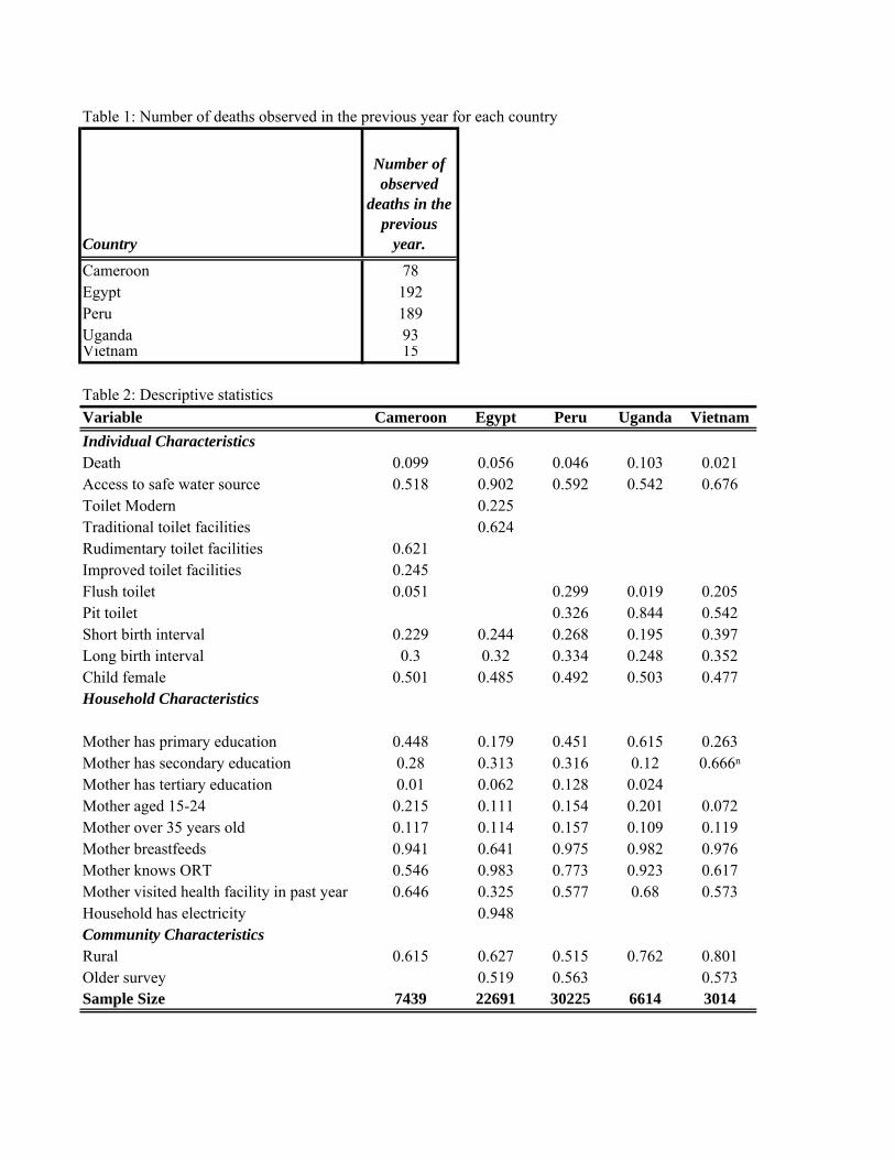
Table 1: Number of deaths observed in the previous year for each country

Country

Number of observed

deaths in the previous

year.

Cameroon 78Egypt 192Peru 189Uganda 93Vietnam 15

Table 2: Descriptive statisticsVariable Cameroon Egypt Peru Uganda VietnamIndividual CharacteristicsDeath 0.099 0.056 0.046 0.103 0.021Access to safe water source 0.518 0.902 0.592 0.542 0.676Toilet Modern 0.225Traditional toilet facilities 0.624Rudimentary toilet facilities 0.621Improved toilet facilities 0.245Flush toilet 0.051 0.299 0.019 0.205Pit toilet 0.326 0.844 0.542Short birth interval 0.229 0.244 0.268 0.195 0.397Long birth interval 0.3 0.32 0.334 0.248 0.352Child female 0.501 0.485 0.492 0.503 0.477Household Characteristics

Mother has primary education 0.448 0.179 0.451 0.615 0.263Mother has secondary education 0.28 0.313 0.316 0.12 0.666ⁿMother has tertiary education 0.01 0.062 0.128 0.024Mother aged 15-24 0.215 0.111 0.154 0.201 0.072Mother over 35 years old 0.117 0.114 0.157 0.109 0.119Mother breastfeeds 0.941 0.641 0.975 0.982 0.976Mother knows ORT 0.546 0.983 0.773 0.923 0.617Mother visited health facility in past year 0.646 0.325 0.577 0.68 0.573Household has electricity 0.948Community CharacteristicsRural 0.615 0.627 0.515 0.762 0.801Older survey 0.519 0.563 0.573Sample Size 7439 22691 30225 6614 3014

Table 3: Water availability stratified by wealth quintilePoorest Second Third Fourth Richest Total

CameroonUnsafe water 1008 1,194 734 377 270 3583

13.55% 16.05% 9.87% 5.07% 3.63% 48.17%Safe water 628 643 787 797 1,001 3856

8.44% 8.64% 10.58% 10.71% 13.46% 51.83%PeruUnsafe water 4813 4,643 1,970 717 185 12328

15.92% 15.36% 6.52% 2.37% 0.61% 40.79%Safe water 2483 2891 4421 4847 3255 17897

8.22% 9.56% 14.63% 16.04% 10.77% 59.21%UgandaUnsafe water 851 814 832 396 135 3028

12.87% 12.31% 12.58% 5.99% 2.04% 45.78%Safe water 707 783 684 710 702 3586

10.69% 11.84% 10.34% 10.73% 10.61% 54.22%VietnamUnsafe water 443 260 149 85 40 977

14.70% 8.63% 4.94% 2.82% 1.33% 32.42%Safe water 326 441 410 387 473 2037

10.82% 14.63% 13.60% 12.84% 15.69% 67.58%

Table 4: Water, sanitation and mortality, possible connectionsProbability of death

Unsafe Water Safe Water No flush Toilet Flush toiletCameroon 11.70% 8.29% 10.10% 6.56%Egypt 8.12% 5.38% 9.05% 5.04%Peru 5.79% 3.73% 5.35% 2.73%Uganda 11.89% 8.95% 10.30% 7.10%Vietnam 3.17% 1.52% 2.33% 0.97%

Table 5: Percentage of children in the baseline scenario Country PercentageCameroon 2.40%Egypt 0.90%Peru 1.70%Uganda 2.00%Vietnam 4.60%

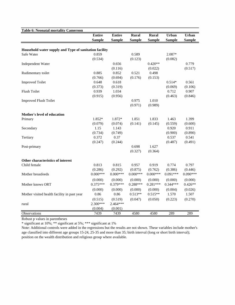
Table 6: Neonatal mortality CameroonEntire Sample

Entire Sample

Rural Sample

Rural Sample

Urban Sample

Urban Sample

Household water supply and Type of sanitation facilitySafe Water 0.859 0.589 2.087*

(0.534) (0.123) (0.082)Independent Water 0.656 0.420** 0.779

(0.116) (0.022) (0.517)Rudimentary toilet 0.885 0.852 0.521 0.498

(0.766) (0.694) (0.176) (0.153)Improved Toilet 0.648 0.618 0.514* 0.561

(0.373) (0.319) (0.069) (0.106)Flush Toilet 0.939 1.034 0.712 0.907

(0.915) (0.956) (0.463) (0.846)Improved Flush Toilet 0.975 1.010

(0.971) (0.989)

Mother's level of educationPrimary 1.852* 1.872* 1.851 1.833 1.463 1.399

(0.079) (0.074) (0.141) (0.145) (0.559) (0.600)Secondary 1.15 1.143 0.920 0.911

(0.734) (0.749) (0.900) (0.890)Tertiary 0.372 0.37 0.537 0.541

(0.247) (0.244) (0.487) (0.491)Post-primary 0.698 1.627

(0.327) (0.364)

Other characteristics of interestChild female 0.813 0.815 0.957 0.919 0.774 0.797

(0.286) (0.292) (0.875) (0.762) (0.386) (0.446)Mother breasfeeds 0.000*** 0.000*** 0.000*** 0.000*** 0.091*** 0.090***

(0.000) (0.000) (0.000) (0.000) (0.000) (0.000)Mother knows ORT 0.375*** 0.379*** 0.288*** 0.281*** 0.344*** 0.426**

(0.000) (0.000) (0.000) (0.000) (0.004) (0.026)Mother visited health facility in past year 0.86 0.86 0.513** 0.515** 1.570 1.507

(0.515) (0.519) (0.047) (0.050) (0.223) (0.270)rural 2.300*** 2.464***

(0.004) (0.001)Observations 7439 7439 4580 4580 289 289Robust p values in parentheses* significant at 10%; ** significant at 5%; *** significant at 1%Note: Additional controls were added in the regressions but the results are not shown. These variables include mother's age classified into different age groups 15-24, 25-35 and more than 35; birth interval (long or short birth interval); position on the wealth distribution and religious group where available.

Table 7: Neonatal mortality EgyptEntire Sample

Entire Sample

Rural Sample

Rural Sample

Urban Sample

Urban Sample

Household water supply and Type of sanitation facilitySafe water 0.659* 0.851 0.259**

(0.067) (0.519) (0.01)Independent water 0.853 1.022 0.419*

(0.412) (0.917) (0.058)Modern Toilet 0.664 0.653* 0.56 0.547 0.5 0.503

(0.113) (0.098) (0.158) (0.143) (0.195) (0.2)Traditional toilet 0.925 0.904 0.977 0.958 0.649 0.636

(0.682) (0.589) (0.91) (0.837) (0.405) (0.386)

Mother's level of educationPrimary 0.723** 0.716** 0.684** 0.676** 0.812 0.796

(0.045) (0.038) (0.049) (0.042) (0.495) (0.455)Secondary 0.913 0.902 0.92 0.902 0.897 0.89

(0.577) (0.527) (0.699) (0.634) (0.68) (0.657)Tertiary 0.692 0.683 1.501 1.467 0.61 0.602

(0.275) (0.258) (0.638) (0.657) (0.221) (0.207)

Other characteristics of interestChild female 0.746*** 0.748** 0.751** 0.752** 0.755 0.752


(0.000) (0.000) (0.000) (0.000) (0.000) (0.000)Mother knows ORT 0.774 0.767 0.553 0.549 1.046 1.061

(0.493) (0.481) (0.269) (0.269) (0.942) (0.923)Mother visited health facility in past year 0.903 0.902 0.894 0.896 0.905 0.906

(0.434) (0.432) (0.516) (0.525) (0.626) (0.63)rural 1.341** 1.356**

(0.048) (0.041)Observations 22691 22692 14231 14231 8460 8460Robust p values in parentheses* significant at 10%; ** significant at 5%; *** significant at 1%

Table 8: Neonatal mortality PeruEntire Sample

Entire Sample

Rural Sample

Rural Sample

Urban Sample

Urban Sample

Household water supply and Type of sanitation facilitySafe water 1.036 1.181 0.845

(0.839) (0.469) (0.539)Independent water 0.89 0.943 0.788

(0.506) (0.814) (0.351)Pit toilet 0.738* 0.744 0.934 0.943 0.457** 0.461**

(0.093) (0.103) (0.771) (0.801) (0.015) (0.017)Flush toilet 0.584** 0.621** 0.753 0.812 0.394*** 0.418***

(0.019) (0.045) (0.596) (0.699) (0.003) (0.007)

Mother's level of educationPrimary 0.835 0.842 0.832 0.841 0.969 1.001

(0.456) (0.477) (0.533) (0.554) (0.952) (0.998)Secondary 0.641 0.652 0.815 0.858 0.704 0.723

(0.117) (0.13) (0.617) (0.704) (0.514) (0.544)Tertiary 0.555* 0.567* 0.35 0.358 0.638 0.657

(0.078) (0.088) (0.178) (0.189) (0.425) (0.453)



(0.000) (0.000) (0.000) (0.000) (0.000) (0.000)Mother knows ORT 0.799 0.801 0.85 0.849 0.824 0.834

(0.181) (0.186) (0.467) (0.463) (0.475) (0.504)Mother visited health facility in past year 1.304* 1.313* 1.313 1.327 1.315 1.317

(0.059) (0.053) (0.199) (0.183) (0.149) (0.147)rural 1.724*** 1.706***

(0.005) (0.005)Observations 30225 30225 15575 15575 14650 14650Robust p values in parentheses* significant at 10%; ** significant at 5%; *** significant at 1%

Table 9: Neonatal mortality UgandaEntire Sample

Entire Sample Rural Sample Rural Sample

Household water supply and Type of sanitation facilitySafe water 1.033 1.852

(0.949) (0.335)Independent water 1.278 1.782

(0.606) (0.473)Pit toilet 0.718 0.774 0.864 0.947

(0.688) (0.757) (0.867) (0.954)Flush toilet 0.159 0.172 3.746 4.76

(0.145) (0.163) (0.142) (0.134)

Mother's level of educationPrimary 1.563 1.62 1.217 1.35

(0.464) (0.431) (0.793) (0.683)Secondary 1.224 1.267

(0.805) (0.773)Tertiary 1.328 1.394

(0.836) (0.805)Post-primary 0.572 0.598

(0.62) (0.657)

Other characteristics of interestChild female 1.195 1.19 1.767 1.783

(0.682) (0.692) (0.317) (0.308)Mother breasfeeds 0.000*** 0.000*** 0.000*** 0.000***

(0.000) (0.000) (0.000) (0.000)Mother knows ORT 0.331 0.336 0.458 0.49

(0.224) (0.232) (0.383) (0.447)Mother visited health facility in past year 0.984 0.968 2.157 1.99

(0.978) (0.956) (0.242) (0.269)rural 1.383 1.416

(0.577) (0.525)Observations 6614 6614 5039 5039Robust p values in parentheses* significant at 10%; ** significant at 5%;*** significant at 1%

Table 10: Neonatal mortality Viet NamEntire Sample

Entire Sample Rural Sample Rural Sample

Household water supply and Type of sanitation facilitySafe water 0.999 0.873

(0.999) (0.743)Independent water 1.115 0.927

(0.774) (0.855)Pit toilet 0.397** 0.392**

(0.022) (0.02)Flush toilet 0.239* 0.234*

(0.099) (0.094)Toilet facility in dwelling 0.416** 0.414**

(0.047) (0.045)

Mother's level of educationPrimary 1.096 1.071 1.309 1.288

(0.905) (0.93) (0.724) (0.74)Post-primary 1.21 1.157 1.191 1.161


(0.35) (0.355) (0.605) (0.606)Mother breasfeeds 0.003*** 0.003*** 0.003*** 0.671***

(0.000) (0.000) (0.000) (0.000)Mother knows ORT 0.716 0.718 0.668 0.671

(0.371) (0.371) (0.338) (0.343)Mother visited health facility in past year 2.549** 2.550** 3.395** 3.399**

(0.018) (0.017) (0.010) (0.010)rural 0.425 0.429

(0.179) (0.182)Observations 3014 3014 2415 2415Robust p values in parentheses* significant at 10%; ** significant at 5%; *** significant at 1%

Table 11: Infant mortality CameroonEntire Sample Entire

SampleRural

SampleRural

SampleUrban Sample

Urban Sample

Household water supply and type of sanitation facilitySafe water 0.673*** 0.696** 0.650

(0.005) (0.028) (0.100)Independent water 0.743* 0.713* 0.885

(0.053) (0.055) (0.686)Rudimentary toilet facilities 1.029 1.007 1.047 1.030

(0.897) (0.975) (0.843) (0.898)Improved toilet 0.889 0.849 0.614* 0.592*

(0.677) (0.566) (0.084) (0.058)Flush toilet 1.025 1.054 0.678 0.669

(0.956) (0.904) (0.42) (0.408)Improved flush toilets 1.241 1.219

(0.475) (0.514)

Mother's Education LevelPrimary 1.289 1.262 1.111 1.086 2.479** 2.471**

(0.121) (0.164) (0.566) (0.653) (0.028) (0.034)Secondary 0.879 0.846 1.630 1.593

(0.576) (0.473) (0.297) (0.327)Tertiary 0.913 0.870 2.142 2.046

(0.916) (0.870) (0.431) (0.456)Post-primary 0.767 0.738

(0.344) (0.280)


(0.744) (0.729) (0.65) (0.64) (0.835) (0.828)Mother Breastfeeds 0.635 0.639 0.762 0.759 0.580 0.582

(0.100) (0.105) (0.514) (0.506) (0.139) (0.139)Mother knows ORT 0.918 0.916 1.08 1.083 0.619* 0.604*

(0.542) (0.531) (0.621) (0.609) (0.074) (0.06)Mother has visited health facility in past year 0.959 0.954 0.884 0.878 1.093 1.104

(0.766) (0.733) (0.451) (0.428) (0.742) (0.712)rural 1.310 1.484**

(0.118) (0.017)Observations 7002 7002 4309 4309 2693 2693Robust p values in parentheses; * significant at 10%; ** significant at 5%; *** significant at 1%

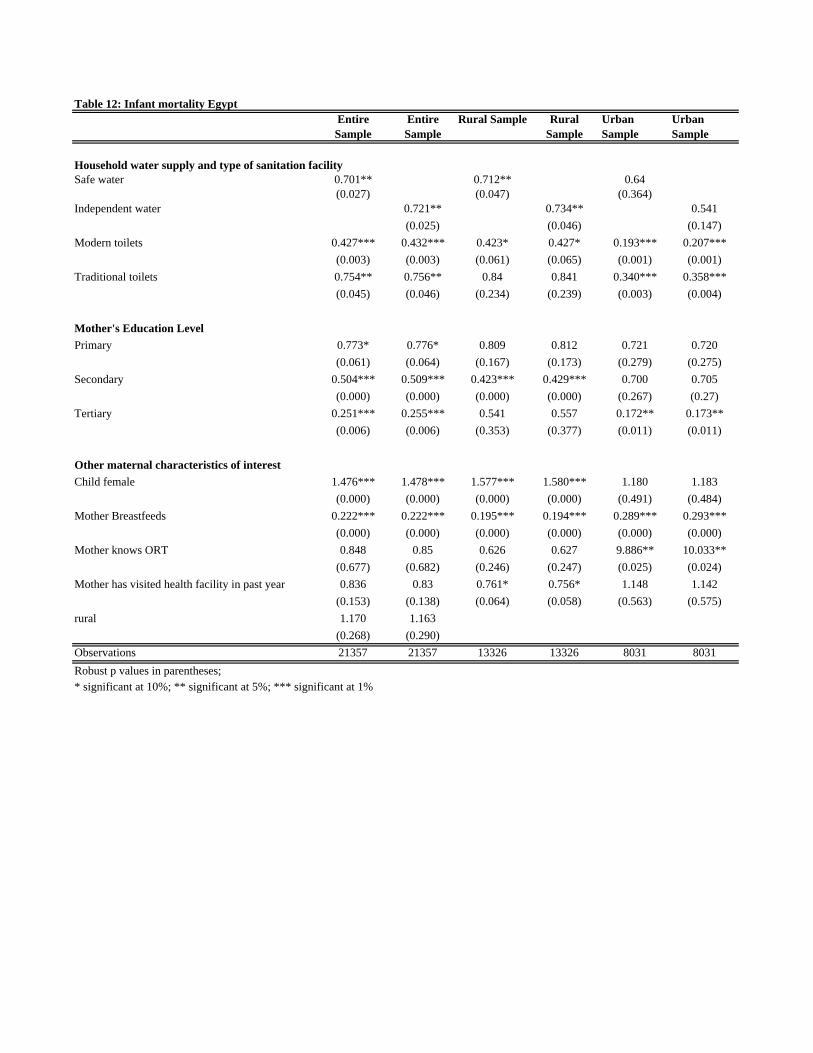
Table 12: Infant mortality EgyptEntire Sample

Entire Sample

Rural Sample Rural Sample

Urban Sample

Urban Sample

Household water supply and type of sanitation facilitySafe water 0.701** 0.712** 0.64

(0.027) (0.047) (0.364)Independent water 0.721** 0.734** 0.541

(0.025) (0.046) (0.147)Modern toilets 0.427*** 0.432*** 0.423* 0.427* 0.193*** 0.207***

(0.003) (0.003) (0.061) (0.065) (0.001) (0.001)Traditional toilets 0.754** 0.756** 0.84 0.841 0.340*** 0.358***

(0.045) (0.046) (0.234) (0.239) (0.003) (0.004)

Mother's Education LevelPrimary 0.773* 0.776* 0.809 0.812 0.721 0.720

(0.061) (0.064) (0.167) (0.173) (0.279) (0.275)Secondary 0.504*** 0.509*** 0.423*** 0.429*** 0.700 0.705

(0.000) (0.000) (0.000) (0.000) (0.267) (0.27)Tertiary 0.251*** 0.255*** 0.541 0.557 0.172** 0.173**

(0.006) (0.006) (0.353) (0.377) (0.011) (0.011)

Other maternal characteristics of interestChild female 1.476*** 1.478*** 1.577*** 1.580*** 1.180 1.183

(0.000) (0.000) (0.000) (0.000) (0.491) (0.484)Mother Breastfeeds 0.222*** 0.222*** 0.195*** 0.194*** 0.289*** 0.293***

(0.000) (0.000) (0.000) (0.000) (0.000) (0.000)Mother knows ORT 0.848 0.85 0.626 0.627 9.886** 10.033**

(0.677) (0.682) (0.246) (0.247) (0.025) (0.024)Mother has visited health facility in past year 0.836 0.83 0.761* 0.756* 1.148 1.142

(0.153) (0.138) (0.064) (0.058) (0.563) (0.575)rural 1.170 1.163


Table 13: Infant mortality PeruEntire Sample Entire

SampleRural

SampleRural

SampleUrban Sample

Urban Sample

Household water supply and type of sanitation facilitySafe water 0.853 0.851 0.796


(0.781) (0.852) (0.601)Pit toilet 0.825 0.816 0.957 0.945 0.503** 0.500**

(0.244) (0.218) (0.809) (0.756) (0.019) (0.017)Flush toilet 0.414*** 0.399*** 1.013 0.97 0.291*** 0.287***

(0.003) (0.002) (0.974) (0.938) (0.002) (0.003)

Mother's Education LevelPrimary 0.767 0.770 0.794 0.795 0.585 0.597

(0.152) (0.157) (0.267) (0.270) (0.171) (0.193)Secondary 0.628* 0.630* 0.651 0.650 0.449* 0.457*

(0.065) (0.067) (0.154) (0.152) (0.073) (0.082)Tertiary 0.669 0.668 0.965 0.955 0.489 0.496

(0.272) (0.268) (0.941) (0.923) (0.199) (0.210)

Other characteristics of interestChild female 0.776** 0.778** 0.887 0.889 0.594** 0.597**


(0.000)) (0.000) (0.002) (0.002) (0.000) (0.000)Mother knows ORT 0.766* 0.768* 0.685** 0.687** 1.152 1.161


(0.910) (0.890) (0.994) (0.994) (0.685) (0.677)rural 1.156 1.179


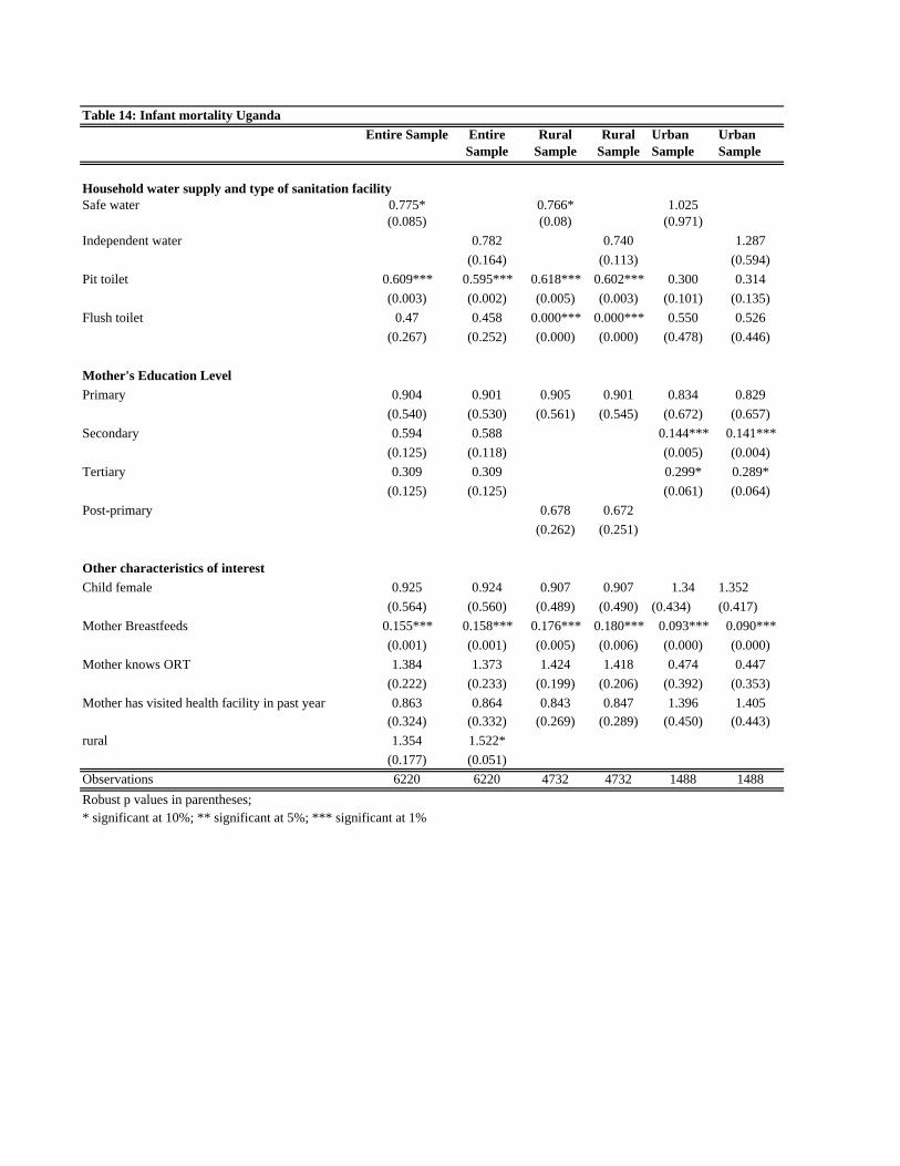
Table 14: Infant mortality UgandaEntire Sample Entire

SampleRural

SampleRural

SampleUrban Sample

Urban Sample

Household water supply and type of sanitation facilitySafe water 0.775* 0.766* 1.025


(0.164) (0.113) (0.594)Pit toilet 0.609*** 0.595*** 0.618*** 0.602*** 0.300 0.314

(0.003) (0.002) (0.005) (0.003) (0.101) (0.135)Flush toilet 0.47 0.458 0.000*** 0.000*** 0.550 0.526

(0.267) (0.252) (0.000) (0.000) (0.478) (0.446)

Mother's Education LevelPrimary 0.904 0.901 0.905 0.901 0.834 0.829

(0.540) (0.530) (0.561) (0.545) (0.672) (0.657)Secondary 0.594 0.588 0.144*** 0.141***

(0.125) (0.118) (0.005) (0.004)Tertiary 0.309 0.309 0.299* 0.289*

(0.125) (0.125) (0.061) (0.064)Post-primary 0.678 0.672

(0.262) (0.251)



(0.001) (0.001) (0.005) (0.006) (0.000) (0.000)Mother knows ORT 1.384 1.373 1.424 1.418 0.474 0.447


(0.324) (0.332) (0.269) (0.289) (0.450) (0.443)rural 1.354 1.522*


Table 15: Infant mortality Viet NamEntire Sample Entire Sample Rural

SampleRural Sample

Household water supply and type of sanitation facilitySafe water 0.219*** 0.208**

(0.007) (0.011)Independent water 0.227*** 0.212**

(0.008) (0.012)Pit toilet 2.383 2.406

(0.373) (0.368)Flush toilet 0.758 0.804

(0.830) (0.868)Toilet facility in dwelling 2.327 2.355

(0.389) (0.384)

Mother's Education LevelPrimary 0.527 0.527 0.523 0.523

(0.507) (0.507) (0.504) (0.506)Post-primary 0.69 0.679 0.631 0.624

(0.634) (0.621) (0.555) (0.546)


(0.55) (0.555) (0.454) (0.453)Mother Breastfeeds 0.059*** 0.059*** 0.051*** 0.051***

(0.002) (0.002) (0.001) (0.001)Mother knows ORT 0.803 0.812 0.925 0.929

(0.694) (0.709) (0.889) (0.896)Mother has visited health facility in past year 0.781 0.788 0.738 0.744

(0.654) (0.665) (0.597) (0.608)rural 2.337 2.676

(0.393) (0.32)Observations 2813 2813 2250 2250Robust p values in parentheses; * significant at 10%; ** significant at 5%; *** significant at 1%

Propensity Score Matching

Table 16: WaterCameroon Egypt Peru Uganda (2000-01)

Survey 2004 Survey 2000

Survey 1995-97

Survey 2000

Survey 1996

Safe water Private water

Private Water Supply 1.08(1.00)

Unsafe water supply 1.04 1.31 1.18 1.35** 1.21** 1.07(0.23) (1.03) (0.99) (2.20) (2.37) (0.54)

Short birth interval 1.1 0.92 0.94 0.70** 0.74** 1.38** 1.35**(0.60) (0.49) (0.53) (2.32) (2.31) (1.97) (2.11)

Long Birth Interval 0.76** 0.69* 0.56*** 0.61*** 0.61*** 0.8 0.78**(2.23) (1.88) (3.51) (2.66) (4.31) (1.03) (2.40)

Child female 0.72* 0.66*** 0.80* 0.72** 0.9 0.73** 0.73*(1.84) (3.27) (1.84) (2.41) (1.13) (2.07) (1.76)

Observations 7416 10798 11778 13167 16987 6594 6562z statistics in brackets

* significant at 10%; ** significant at 5%; *** significant at 1%

Table 17: Sanitation Egypt Peru

Survey 2000Survey

1995-97Survey 2000

Survey 1996

Modern Toilet Facilities 0.75* 0.67**(1.72) (2.10)

No Toilet Facilities 1.25* 1.47***(1.70) (3.77)

Birth Interval 0.95 0.98 0.60*** 0.75**(0.35) (0.13) (2.88) (2.00)

Long Birth Interval 0.71** 0.57*** 0.61*** 0.61***(2.27) (3.72) (2.97) (3.89)

Child female 0.64*** 0.81* 0.73** 0.91(3.78) (1.66) (2.21) (0.97)

Observations 10783 11765 13179 17000z statistics in brackets

* significant at 10%; ** significant at 5%; *** significant at 1%

Documents

Human Development Report 2006hdr.undp.org/sites/default/files/fuentes_et_al_a.pdfHuman Development Report 2006 ... urban/rural differences in the infant mortality rate ... estimation