1

Chapter 6

Human Capital

Copyright © 2010 The McGraw-Hill Companies, Inc. All rights reserved.McGraw-Hill/Irwin

Labor Economics, 5th edition

7 - 2

Introduction

W i d b diff k l diff b f• Wages received by different workers not only differ because of compensating wage differentials, but also because different workers bring into the labour market unique sets of abilities and acquired skills known as human capital.

• Workers add to their stock of human capital throughout their lives (“life-long learning”), especially through formal and ( g g ), p y ginformal education and job experience.

• How do workers choose what skills to acquire, and how does that affect earnings?

2

7 - 3

Introduction ctd.

• Basic trade-off: People receive lower or no earnings during d ti d t i i b t h t i hi h i l teducation and training, but hope to receive higher earnings later

due to their increased human capital. But is it a good investment?

• Basic assumption: A person chooses the level of human capital investments that maximises the present value of lifetime earnings. g

• Note that this is not the only determinant of a person’s income. Human capital cannot explain everything (but possibly a lot). Luck also plays a role in ‘real life’.

7 - 4

6-1 Education in the Labour Market: Some Stylized Facts

d i i l l d i h• Education is strongly correlated with:- Labour force participation rates.- Unemployment rates.- Earnings.

This applies to NZ as well as the US. pp

• Some NZ statistics from Statistics NZ’s “Labour Market Statistics 2007” where shown in class.

3

7 - 5

6-2 Present Value

• Present value (PV) allows comparison of dollar amounts spentPresent value (PV) allows comparison of dollar amounts spent and received in different time periods.

PV = y/(1+r)t

- PV is the present value of y dollars received t years from now. - r is the discount rate.

7 - 6

6-3 The Schooling Model

• The basic assumption (i.e. maximisation of the PV of lifetime earnings) is quite strong! Education & training are valued onlyearnings) is quite strong! Education & training are valued onlybecause they increase earnings!

- Non-monetary rewards of ‘schooling’ are neglected for simplicity. But there are many of these!

• A simple model: - 18 year old who finished high-school: To go or not to go to

university for four years? - Assume for simplicity there is no on-the-job training if s/he joins

the workforce instead of going to university. Also, assume skills learned at school do not depreciate over time. In that case, the person’s productivity does not change after leaving school and his/her real income stays constant over the life-cycle.

4

7 - 7

Figure 6-1: Potential Earnings StreamsFaced by a High School Graduate

Dollars

wCOL

wHS

Goes to College

Quits After High School

A person who quits school after getting his/her high school diploma can earn wHS from age 18 until the age of retirement. If s/he decides to go to college, /h f th i

18 6522Age

-H

0

s/he foregoes these earnings and incurs a cost of Hdollars for 4 years and then earns wCOL until retirement age.

7 - 8

The Schooling Model ctd.

• Real earnings (earnings adjusted for inflation)• Real earnings (earnings adjusted for inflation).• Figure 6.1 shows two age-earnings profiles – the two wage

profiles over the person’s (work) lifespan.

• Going to university involved two types of costs:- Foregone earnings (opportunity costs of 4 years wages at wHS).- Direct costs while studying (H): Fees, books etc.

• Calculate the PVs of the person’s two potential lifetime income streams. See equations (6.4) and (6.5), Borjas, p. 241.

5

7 - 9

The Schooling Model ctd.

• WCOL has to be greater than wHS or no person would go to university (the higher wage is like a compensating differential for the higher training costs).Equation (6.6): Go to College if PVCOL > PVHS

• The discount rate is usually crucial: The higher the discount rate, the less likely someone will invest in education (since th l f t i t d)they are less future oriented).

• The discount rate depends on:- The market rate of interest.- The individual’s “time preference” (how a person feels about

giving up today’s consumption in return for future rewards).

7 - 10

The Wage-Schooling Locus

• The comparison of PVs can be generalized to more than two options, e.g. hi h h l d d d d h fhigh-school, undergraduate versus graduate degree, or each year of schooling.

• Another approach to determine the optimal length of schooling is to draw a wage-schooling locus. This locus shows what salary firms are willing to pay a particular worker for given levels of schooling. It is market determined!

• Three properties of the wage-schooling locus:It is upward sloping (more educated workers earn more)- It is upward sloping (more educated workers earn more).

- The slope of the wage-schooling locus indicates the increase in earnings associated with one more year of schooling.

- The wage-schooling locus in concave (diminishing returns to education are assumed).

• Do you think these properties always apply?

6

7 - 11

The Wage-Schooling Locus

The wage-schooling locus Dollars

g ggives the salary that a particular worker would earn if s/he completed a particular level of schooling. If the worker graduates from high school, s/he earns $20,000

30,000

20,000

23,00025,000

annually. If s/he goes to university for 1 year, s/he earns $23,000.

(Note that in the US high school finished after year 12)

0 13 14 1812 Years of Schooling

7 - 12

The Marginal Rate of Return to Schooling

• The slope of the wage-schooling locus (Δw/ Δs) tells us the• The slope of the wage-schooling locus (Δw/ Δs) tells us the increase in earnings for one more year of schooling.

• The marginal rate of return (MRR) to schooling is the percentage change in earnings resulting from one more year of schooling.

MRR: (Δw/w)*100

The MRR declines with more years of schooling.

The MRR gives the percentage increase in earnings per $ spent in educational investment (see p. 244).

7

7 - 13

Figure 6-3: The Schooling Decision

Rate of The MRR schedule gives the Rate of Discount

r′

r

gmarginal rate of return to schooling.

The stopping rule for schooling investments:

A worker maximizes the present value of lifetime earnings by

i t h l til th MRR t

Years of Schoolings*s′

MRR

going to school until the MRR to schooling equals the rate of discount. A worker with discount rate r goes to school for s* years. A worker with a higher discount rate goes to school for fewer years.

7 - 14

6-4 Education and Earnings

• Observed data on earnings and schooling do not allow us to estimate returns to schooling.

• In theory, a more able person gets more from an additional year of education.

• Ability bias – the extent to which unobserved ability diff i t ff t ti t t t h li ( idifferences exist affects estimates on returns to schooling (since the ability differences, and not the length of schooling, may be the true source of the wage differentials). If there is an ability bias, different workers have different wage-schooling loci.

8

7 - 15

MRR if Workers Differ Only in Terms of Their Discounts Rates

• Case 1:Case 1: If workers differ only in terms of their discount rates, it is easy to estimate the returns to schooling:

- They lie on different points of the same wage-schooling locus and have the same MRR schedule (Figure 6-4)

- We can use the observed wage differential wHS – wDROP to calculate the MRR:

MRR = (wHS – wDROP) / wDROP

7 - 16

Figure 6-4: Schooling and Earnings When Workers Have Different Rates of Discount (Case 1)

Rate of Interest Dollars

rBO

rAL

MRR

wDROP PAL

PBO

wHS

Years of Schooling

Years of Schooling

1212 1111

MRR

9

7 - 17

Returns to Schooling and Ability Bias

• Case 2:It is much more difficult to estimate returns to schooling when all workers have the same discount rate, but each faces a different wage-schooling locus because of differences in unobserved ability that result in different MRR schedules. (Unobserved ability means we have no data on ability differences between workers)

- See Figure 6-5: Bob is more productive than Ace. Bob earnsSee Figure 6 5: Bob is more productive than Ace. Bob earns more than Ace even if both have the same level of schooling.

This has important policy implications: More schooling alone will not increase earnings of the less able to the level of the more able workers!

7 - 18

Figure 6-5: Schooling and Earnings When Workers Have Different Abilities (Case 2)

Rate of Interest Dollars ZInterest

r

MRR

MRRBOB

wHS

wACE

PACE

wDROP

ZBob

Ace

Years of Schooling

Years of Schooling

1211

MRRACE

1211

Ace and Bob have the same discount rate (r) but each worker faces a different wage-schooling locus. Ace drops out of high school and Bob gets a high school diploma. The wage differential between Bob and Ace (or wHS - wDROP) arises both because Bob goes to school for one more year and because Bob is more able. As a result, this wage differential does not tells us by how much Ace’s earnings would increase if he were to complete high school (or WACE – wDROP).

10

7 - 19

6-5 Estimating the Rate of Return to Schooling

• A typical study estimates a regression of the form:

log(w) = bs + other variables

• w is the worker’s wage • s is the years of schooling acquired by the worker• b is the coefficient that estimates the rate of return to

one additional year of schooling (assuming that the ‘other variables’ control for all other differences between workers, including any differences in ability). However, we can never be sure that ‘all other differences’ are controlled for.

- “Consensus’ estimate of about 9 % for MRR.

7 - 20

How to control for ‘other differences’?

In order to get around this problem, various approaches have o de to get a ou d t s p ob e , va ous app oac es avebeen used:

- ‘Natural experiments’: Use data on identical twins! In studies of twins, presumably holding ability constant, valid estimates of MRR to schooling can be estimated.• Mixed results (MRR between 3-15%)! Identical twins

not really identical.

- Using instrumental variables generated by government policies (MRR about 7.5%).

11

7 - 21

6-7 Policy Application: School Quality and Earnings

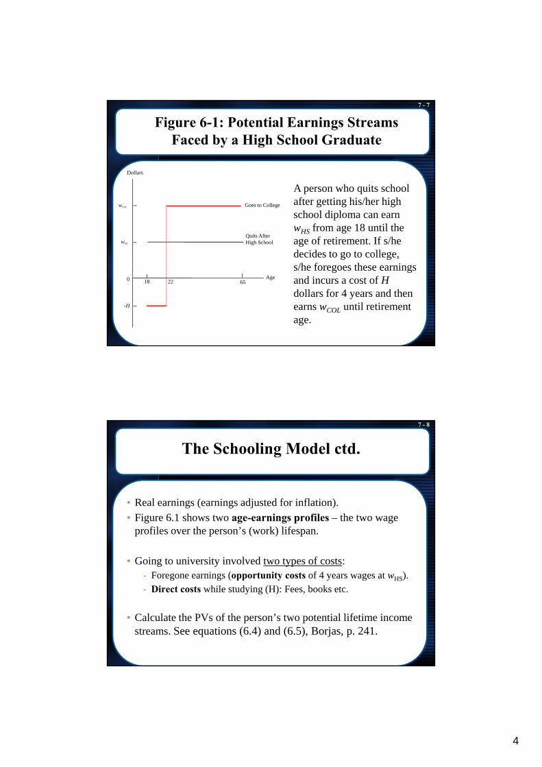
• Review of the history of the US debate about whether schooling• Review of the history of the US debate about whether schooling quality increases earnings.

• Card & Krueger (1992): Schooling quality as measured by class size negatively affects the MRR to education, whereas teachers’ earnings affect it positively .

• Generally they found the rate of return to schooling higher for• Generally, they found the rate of return to schooling higher for workers who were born in US states with well-funded education systems.

• Briefly discussed NZ school funding, e.g. low decile schools receive higher government funding.

7 - 22

Figure 6-6: School Quality and the Rate of Return to Schooling

8g 8ng

2

3

4

5

6

7

15 20 25 30 35 40

Pupil/teacher ratio

Rate

of r

etur

n to

sch

oolin

2

3

4

5

6

7

0.5 0.75 1 1.25 1.5 1.75 2

Relative teacher wage

Rat

e of

ret

urn

to s

choo

li

p

Source: David Card and Alan B. Krueger, “Does School Quality Matter? Returns to Education and the Characteristics of Public Schools in the United States,” Journal of Political Economy 100 (February 1992), Tables 1 and 2. The data in the graphs refer to the rate of return to school and the school quality variables for the cohort of persons born in 1920-1929.

12

7 - 23

6-8 Do Workers Maximize Life-Time Earnings?

• The schooling model assumes that workers select their level of d ti t i i th t l f lif ti ieducation to maximize the present value of lifetime earnings.

• The only way to test this hypothesis is if we can observe the age-earnings profile of a worker in two ways: If s/he chooses college, or if s/he stops education investments after finishing high school.

U f t t l h i i d t b th• Unfortunately, once a choice is made, we cannot observe the earnings stream associated with the non-choice.

• Thus, using the observed wage differential to determine if the worker selected the “right” earnings stream yields meaningless results. “Selection Bias”

7 - 24

Self-Selection Bias

• Workers may select themselves into jobs for which they are Wo e s ay se ect t e se ves to jobs o w c t ey a ebetter suited (see numerical example, p. 260/1), i.e. for which they have a comparative advantage.

• Therefore, wage differentials may not be associated with education, but different abilities which are not due to education.

• Then what is the point of investing in higher education? For h i ’ !some, there isn’t any!

• There are econometric techniques that correct for the selection bias. Models that use them seem to confirm the theory that people choose the schooling option that maximizes the PV of lifetime earnings.

13

7 - 25

6-9 Schooling as a Signal

Alt ti i t th t f th H C it l d l Ed ti• Alternative view to that of the Human Capital model: Education does not increase productivity but acts as a signal:

- The employer cannot properly observe a worker’s ability directly. An education qualification (e.g. university degree) acts as a signal that the person is likely to have the abilities and qualities required to become a productive worker!

• Often used by university lecturers to justify boring lectures: If students can cope with that, they can cope with working life!

• Using positive spin, one could say instead that if students are able and motivated enough to pass university, they are likely to cope with jobs.

7 - 26

Schooling as a Signal ctd.

• Why use signaling? From the high productivity worker’s ti i li i t id ‘ liperspective, signaling is necessary to avoid a ‘pooling

equilibrium’ (p. 263) which results in lower wages for them (i.e. employers pool high- and low-productivity workers and pay an average wage below what high-productivity workers are worth).

• Instead, there could be a “separating equilibrium” (also see , p g q (numerical example pp. 264-266).

- Low-productivity workers choose not to obtain X years of education, voluntarily signaling their low productivity.

- High-productivity workers choose to get at least X years of schooling and separate themselves from the pack.

14

7 - 27

Figure 6-7: Education as a Signal

Dollars

Costs

Dollars

300,000

25,001y−

20,000y−

200,000

0 Years of

Costs

Slope = 25,001

300,000

200,000

0 Years of

Costs

Slope = 20,000

y− y−

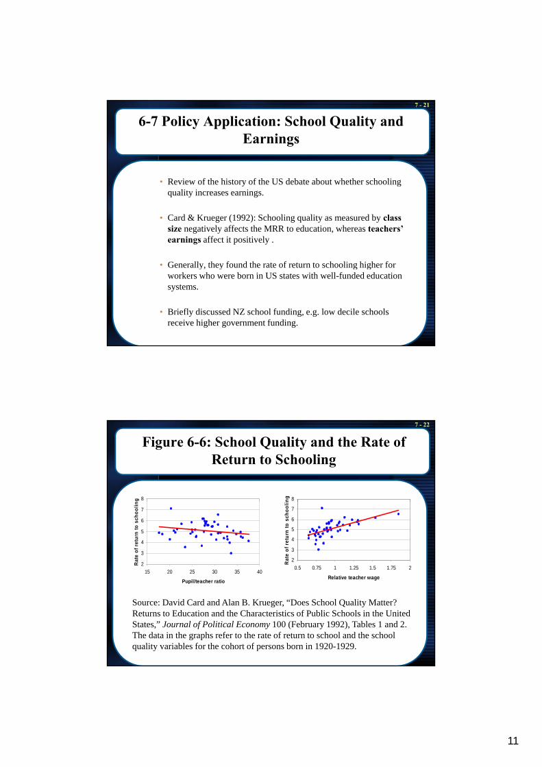
Workers get paid $200,000 if they get less than y− years of college, and $300,000 if they get at least y− years. Low-productivity workers find it more expensive to invest in college, and will not get y− years. High-productivity workers do obtain y− years. As a result, the worker’s education signals if s/he is a low-productivity or a high-productivity worker.

0 Years of Schooling

0 Years of Schooling

(a) Low-Productivity Workers

y y

(b) High-Productivity Workers

7 - 28

Implications of Schooling as a Signal

• Crucial assumption of the “schooling as a signal model”: Low-C uc a assu pt o o t e sc oo g as a s g a ode : owproductivity workers find it more costly than high-productivity workers to obtain the signal (and therefore do not obtain it).

• Very difficult to establish empirically if education plays a productivity enhancing role (human capital model), a signaling role (signaling model), or both. BOTH theories imply that more educated workers earn higher wages. g g

• It is important for many policy questions to know the extent to which each model applies!

• If the signaling model applies, there is a positive private rate of return to schooling, but the social rate of return is zero!

15

7 - 29

Private and Social Rates of Return to Schooling

• Private rate of return to schooling: The percentage increase in a worker’s earnings resulting from an additional year of schooling.

• Social rate of return to schooling: The percentage increase in national income resulting from an additional year of schooling.

• However, the social rate of return is still likely to be positive even if a particular worker’s human capital is not increased by schooling because signaling sorts workers into the right jobs, i.e. it reduces the costs of worker and job mismatches!

• One can also argue that the ‘social rate of return’ should include the impact of education on things other than earnings (like civic engagement, reduction in crime, attitudes towards democracy, acceptance of new ideas & technology, etc.).

7 - 30

Some Empirical Findings on Rates of Returnto Education

Some NZ and international findings:

• Maani, S. (1996), “Private and social rates of return to secondary and higher education in New Zealand: Evidence from the 1991 census”, Australian Economic Review, 113, 1st Quarter 1996, 82-100. (330 Aus)

• Gibson, J. (2000), “Sheepskin effects and the return to education in New Zealand: Do they differ by ethnic group?”, New Zealand Economic Papers, 34(2), 201-220. (330.993 New)

• Maani, S. and T. Maloney (2004), “Returns to post-school qualifications: New evidence based on the HLFS Income Supplement (1997-2002)” Report to theevidence based on the HLFS Income Supplement (1997 2002) , Report to the Labour Market Policy Group, Department of Labour, Wellington. http://www.dol.govt.nz/PDFs/PostSchoolQuals.pdf

• Nair, B. (2007), Measuring the Returns on Investment in Tertiary Education Three and Five Years After Study, Ministry of Education, Wellington.

• Psacharopoulos, G. and H. A. Patrinos (2004), “Returns to investment in education: A further update”, Education Economics, 12 (2), 111-134. (379 Edu)

16

7 - 31

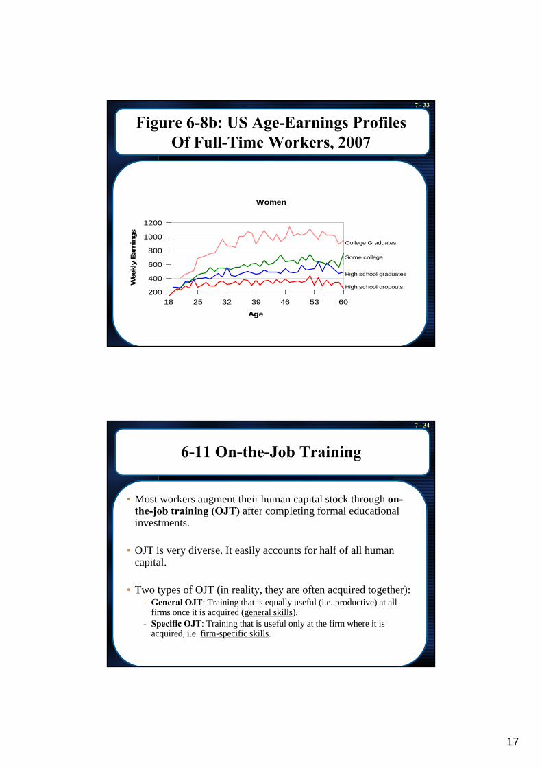
6-10 Post-School Human Capital Investments

• Three important properties of age-earnings profiles:• Three important properties of age-earnings profiles:- Highly educated workers earn more than less educated workers.- Earnings rise over time at a decreasing rate.- The age-earnings profiles of different education cohorts diverge over time (they

“fan outwards”), i.e. earnings increase faster for more educated workers.

• Some NZ evidence from:- Maani, S. (1996), “Private and social rates of return to secondary and higher , ( ), y g

education in New Zealand: Evidence from the 1991 census”, Australian Economic Review, 113, 1st Quarter 1996, 82-100. (330 Aus)

- Le, T., Gibson, J, and L. Oxley (2006), “A forward-looking measure of the stock of human capital in New Zealand”, Manchester School, 74(5), 593-609. (330 Man)

7 - 32

Figure 6-8a: US Age-Earnings Profiles Of Full-Time Workers, 2007

110014001700200023002600

kly

Earn

ing

s

Men

Some college

College Graduates

200500800

1100

18 25 32 39 46 53 60

Week

Age

Some collegeHigh school graduatesHigh school dropouts

17

7 - 33

Figure 6-8b: US Age-Earnings Profiles Of Full-Time Workers, 2007

Women

600

800

1000

1200

y Ea

rnin

gs

Some college

College Graduates

200

400

600

18 25 32 39 46 53 60

Age

Wee

kly

High school graduates

High school dropouts

7 - 34

6-11 On-the-Job Training

• Most workers augment their human capital stock through on-ost wo e s aug e t t e u a cap ta stoc t oug othe-job training (OJT) after completing formal educational investments.

• OJT is very diverse. It easily accounts for half of all human capital.

• Two types of OJT (in reality, they are often acquired together):- General OJT: Training that is equally useful (i.e. productive) at all

firms once it is acquired (general skills).- Specific OJT: Training that is useful only at the firm where it is

acquired, i.e. firm-specific skills.

18

7 - 35

A Simple Model of OJT

• A worker is employed by a firm for two periods. The firm’s hiring condition is:

TC1 + TC2/(1+r) = VMP1 + VMP2/(1+r) (6-21)

• TC is the wage plus any other cost involved in employing the worker. Assume there is OJT in the first period (at a cost of H $s):)

w1 + H + w2/(1+r) = VMP1 + VMP2/(1+r) (6-22)

• If OJT is general, the firm will have to pay a wage in the second period equal to the now higher VMP2 (because the worker could earn this at other firms). Use w2=VMP2 in (6-22):

7 - 36

A Simple Model of OJT ctd.

w1 = VMP1 – H (6-23)

• (6-23) implies that the worker has to accept a lower wage in the first period to get the general OJT. Workers pay for general OJT, competitive firms do not.

• What if OJT is specific? In this case, the worker’s alternative wage in period 2 is independent of the OJT and equals the pre-training wage. Two cases two consider:

19

7 - 37

A Simple Model of OJT ctd.

• Case A: Assume the firm paid for specific OJT. - To recoup the training costs, the firm could keep the wage low in

period 2 (i.e. below VMP2).• To do this, the firm has to have some assurance that the worker,

once trained, does not leave the firm. Otherwise the firm would suffer a loss (i.e. the training cost).

• Case B: Assume the worker paid for specific OJT.- The worker gets a lower wage in period 1, and a higher wage in

period 2. • To accept this, the worker has to have some assurance that the firm

will employ him/her in period 2. Otherwise the worker will lose the investment in OJT.

• To summarise, both firms and workers are reluctant to invest in specific OJT.

7 - 38

A Simple Model of OJT ctd.

• The way out of this dilemma:• The way out of this dilemma:- Fine-tune the post-training wage to reduce the probabilities of

both quits and layoffs:Set the post-training (period 2) wage so that the firm and the worker share the returns to specific training:

• Set it somewhere between the alternative wage that the worker could earn at other firms and his/her VMP2.

• In that case, the firm has no incentive to lay-off the worker (theIn that case, the firm has no incentive to lay off the worker (the firm pays the worker less than VMP2) and the worker has no incentive to quite (s/he receives a wage larger than the alternative wage).

• Firms and workers sharing the benefits of specific OJT also implies that they share the costs of it (i.e. 30% of costs and 30% of benefits for one, 70% of each for the other)!

20

7 - 39

Some Implications of Specific OJT

• Specific OJT breaks the link between the worker’s wage and VMP throughout his/her life cycle and creates a kind of ‘lifetime employmentthroughout his/her life-cycle and creates a kind of lifetime employment contract’.

• The model can explain the ‘last hired, first fired’ rule: The workers last hired have less specific OJT (and therefore less of a gap between the wage and their VMP). Workers with more specific OJT have a larger ‘buffer’ between their wage and their VMP.

- When there is a downturn, VMP falls. Workers with longer tenure are more ‘protected’more protected .

• The model can explain temporary layoffs of (older) workers with more firm-specific OJT. They tend to wait longer to get re-hired by the same firm.

• Specific OJT can explain the negative correlation between job turnover and job seniority.

7 - 40

6-12 On-the-Job Training and the Age-Earnings Profile

• OJT affects wages and therefore the shape of the age-earnings function.

• When during a working life should OJT take place? Rule: In every time period invest in human capital through OJT up to the point where Marginal Revenue equals Marginal Cost of the investment.

• How do MR and MC of investment in OJT change over time?• A simple model:

- Human capital measured in ‘efficiency units’ (standardised units of- Human capital measured in efficiency units (standardised units of human capital).

- These ‘efficiency units’ can be rented out in the labour market at a rate of R dollars.

- Assume the market for ‘efficiency units’ is competitive. R is the same for each unit.

- Assume general OJT and no depreciation of human capital!

21

7 - 41

Another Simple Model

- Assume a worker starts work at age 20 and plans to retire at age 65. g p gThe MR of acquiring one efficiency unit of human capital at age 20 is:

MR20 = R + R/(1+r) + R/(1+r)2 … + R/(1+r)45 (6-25)

- MR of acquiring one efficiency unit of human capital at age 30 is:

MR = R + R/(1+r) + R/(1+r)2 + R/(1+r)35 (6 26)MR30 = R + R/(1+r) + R/(1+r)2 … + R/(1+r)35 (6-26)

- MR30 is smaller than MR20 (10 fewer terms), assuming the worker still plans to retire at age 65.

- The model implies that human capital investments are more profitable the earlier they are made. But are they always?

7 - 42

Another Simple Model ctd.

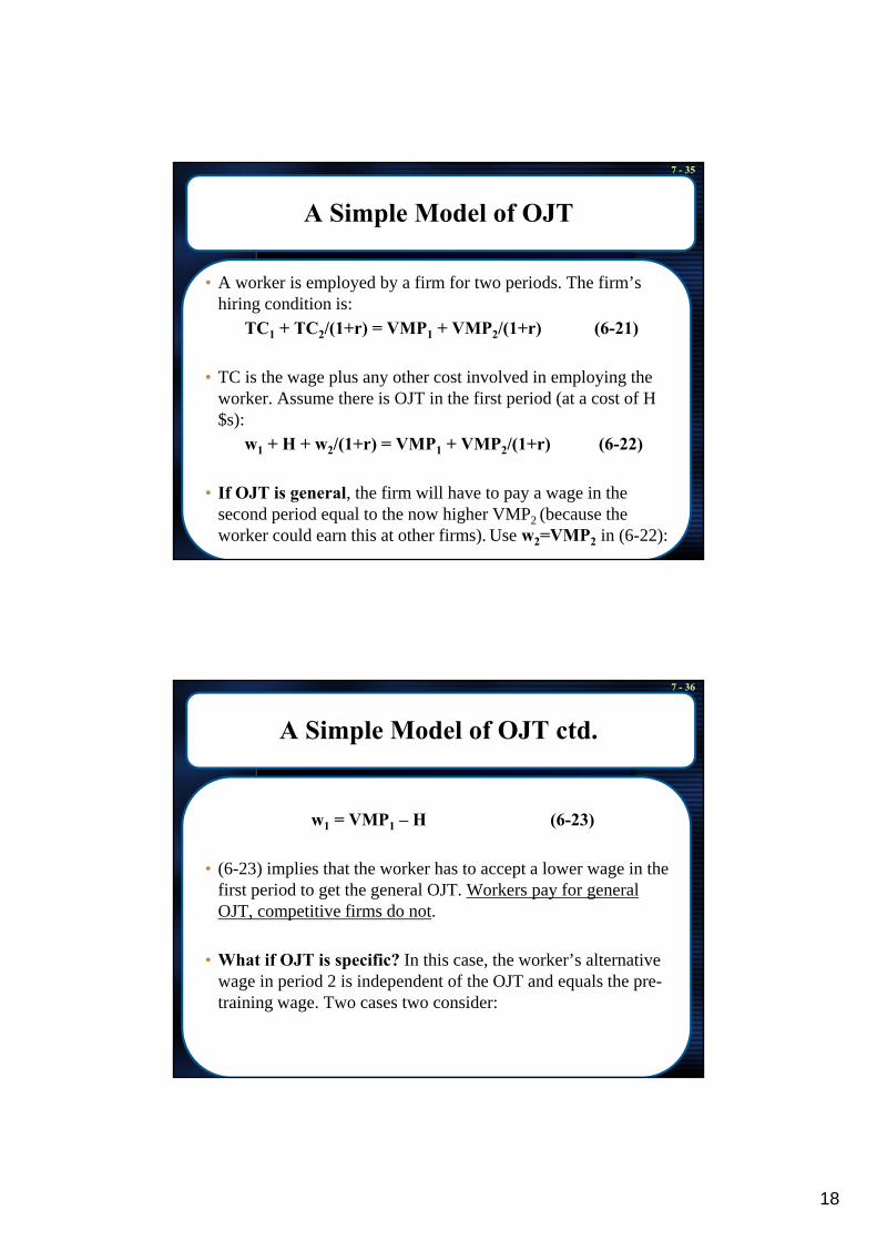
• What about the MC of acquiring an extra efficiency unit of human capital? It is assumed that MC rise as morehuman capital? It is assumed that MC rise as more efficiency units are acquired.

- Do they really? We are not talking about formal education which involves tuition fees etc. Also see footnote 42, p. 276.

• The simplified assumptions of the model allow us to draw some ‘common sense’ conclusions, e.g. that the worker acquires fewer efficiency units as s/he gets older. See Figure 6-9.Figure 6 9.

- What about life-long learning? The increase in ‘knowledge work’ has made this necessary for more and more workers.

• Because the worker acquires more human capital when young, his/her age-earnings profile is upward sloping (see Figure 6-10).

22

7 - 43

Figure 6-9: The Acquisition of Human Capital over the Life Cycle

Dollars The marginal revenue of ffi i it f

MC

MR20

MR30

an efficiency unit of human capital is assumed to decline as the worker ages (so that MR20, the marginal revenue of a unit acquired at age 20, lies above MR30). At each age, the worker equates the

0 Q30 Q20

Efficiency Units

qmarginal revenue with the marginal cost, so that more units are acquired when the worker is younger.

7 - 44

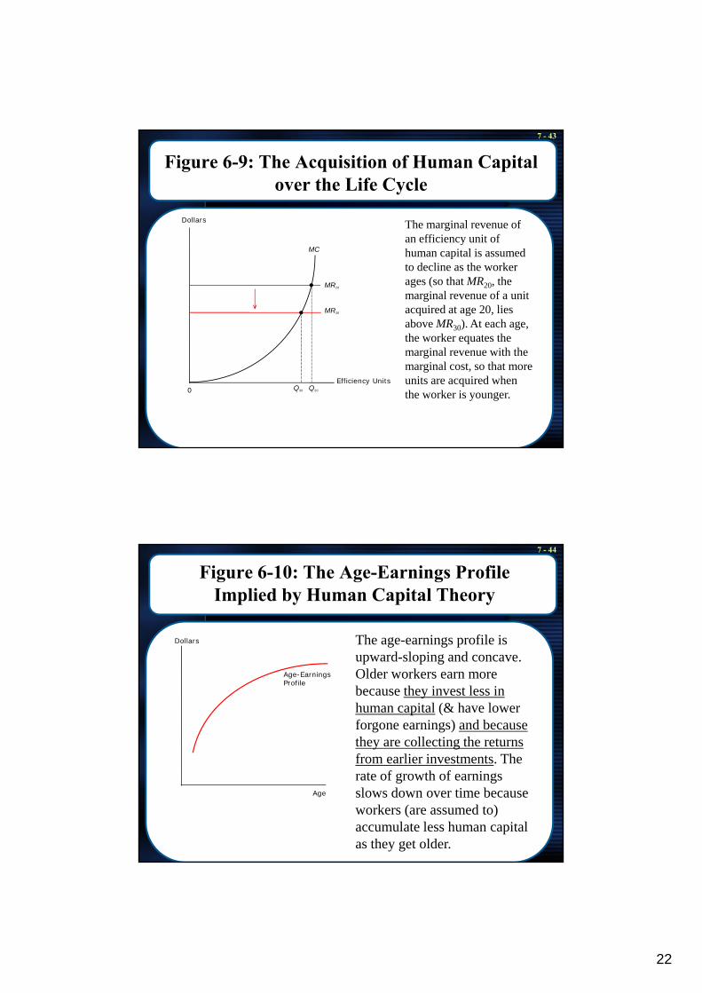
Figure 6-10: The Age-Earnings Profile Implied by Human Capital Theory

Dollars The age-earnings profile is

Age-Earnings Profile

upward-sloping and concave. Older workers earn more because they invest less in human capital (& have lower forgone earnings) and because they are collecting the returns f li i t t Th

Age

from earlier investments. The rate of growth of earnings slows down over time because workers (are assumed to) accumulate less human capital as they get older.

23

7 - 45

The Mincer Earnings Function

• Jacob Mincer showed that the human capital model t i f ti f th fgenerates age-earnings functions of the form:

Log(w) = a∗s + b∗t – c∗t2 + other variables (6-27)

w = wage; s = years of formal education; t = years of job experience; t2 takes care of non-linearity of the function.

‘a’ estimates the rate of return to formal schooling (if the ability bias is controlled for).

‘b’ & ‘c’ estimate the importance of OJT (its impact on earnings).

• Hundreds of studies have estimated such Mincer earnings functions. Formal education & OJT seem to explain about one third of the variation in wages.

7 - 46

6-13: Policy Application: Evaluating Government Training Programmes

• The discussion, although US-specific, is instructive for anyone interested in g p ythe evaluation of training and employment policies.

- The human capital model implies that training unskilled workers can substantially improve their economic welfare. How can such training programmes be evaluated?

- Because of self-selection bias, before and after comparisons of income (and associated rates of return) are meaningless.

‘R l ti ’ hift i li l ti i th U S t d d i d- ‘Revolutionary’ shift in policy evaluation in the U.S. towards randomized experiments (see pp. 279-81 and Table 6-4). They seem to suggest that the rate of return to government training programmes is around 10%.

- But even randomised experiments can be criticized because the self-selection bias may still be present.

24

7 - 47

Policy Evaluation

F i f ti th NZ it ti• For information on the NZ situation see: - Johri, R., de Boer, M. Pusch, H., Ramasamy, S. and K. Wong (2004),

Evidence to date on the working and effectiveness of ALMPs in New Zealand, Department of Labour and Ministry of Social Development, Wellington. http://www.msd.govt.nz/about-msd-and-our-work/publications-resources/evaluation/evidence-effectiveness-almps-nz/

• The paper provides an overview of active labour market policies (ALMPs) in NZ. Johri et al. state that randomised experiments have not yet been used in NZ. Instead, they use a ‘quasi-experimental’ method:

- This involves selecting a treatment and control group after the policy intervention (in randomised experiments the two groups are selected before policy intervention).

7 - 48

Policy Evaluation

• Johri et al. find there is no ‘golden bullet’ or single programme g g p gwhich will be successful for all job seekers. Most programmes are effective for some participants.

• For a summary of the findings on the effectiveness of various ALMPs, see Johri et al., Table 11, p. 38.

• The NZ findings are consistent with international findings (see g g (Johri et al., Table 14, p.41).

End of Chapter 6