Embed Size (px)
Citation preview
1
ISSN 1833-4474
Human Capital Inequality and the Kuznets Curve
Audrey Siew Kim LIM and Kam Ki TANG*
School of Economics
University of Queensland
March 2006
Summary � This paper develops a measure of human capital distribution. Based on a
Mincer specification of human capital, the measure takes into consideration years of
schooling, school dropouts, differential rates of returns to schooling, and education quality.
We apply the proposed measure to evaluate national and global human capital inequality
and compare them with education inequality measures. Human capital Kuznets curves are
evident when relative inequality measures are used while education Kuznets curves are
found when absolute inequality measures are used. It is also found that while global
education inequality has been declining over the past four decades, global human capital
inequality remains largely steady.
Key words: education, human capital, inequality, Kuznets curve
JEL Classification: D63, I32, O15
* Corresponding author. Address: School of Economics, University of Queensland, QLD 4072, Australia. Telephone: +617 3365 9796. Fax: +617 3365 7299. Email: [email protected]. The authors wish to acknowledge helpful suggestions from Jongwha Lee, D.S. Prasada Rao, James Laurecenson, Alicia Rambaldi, Phil Bodman and Derek Headey on earlier versions of the paper.
2
1. INTRODUCTION
This paper focuses on the measurement of human capital inequality. In the vast
majority of the empirical growth literature, emphases have been put solely on the average
level of human capital of nations, especially the capital derived from investments in
education (e.g. see Barro 2001; Krueger & Lindahl 2000; Mankiw, Romer & Weil 1992).
The impact of the distribution of human capital has not received much attention until very
recently. For instance, Thomas, Wang and Fan (TWF) (2000) and Castelló and Doménech
(2002) examine the relationship between human capital inequality and growth across
countries, whereas Checchi (2001) and De Gregorio and Lee (2002) investigate the linkage
between human capital inequality and income inequality.
It is important to consider the distribution of human capital in addition to the average
quantity of human capital in studying growth or development for a number of reasons.
Firstly, human capital, unlike other types of capital, is not perfectly tradable; hence, its
marginal product across individuals is not equalized. This gives rise to aggregation
problems and thus aggregate output no longer depends merely on the average level of the
human capital, but also on its distribution (TWF2002). Secondly, the distribution of human
capital is determined by individual ability and investment financing opportunities, and this
distribution is an approximate determinant of the distribution of earnings. Thus, if a
population�s abilities are normally distributed, a skewed distribution of education services
would potentially cause great welfare losses (Mincer 1974). Thirdly, since human capital is
a key determinant of not only current and but also future income, measures of human capital
inequality can provide a leading indicator of income inequality and aid policymakers in
developing income transfer programs if the situation requires.
While there is a growing interest in studying the impacts of human capital inequality
on growth and development, the measurement of human capital inequality has not yet been
3
properly constructed. For instance, in the studies cited above, education inequality is used
as a proxy of human capital inequality, and education quality is not accounted for. Our
survey of the literature shows that although the literature on measuring the average level of
human capital has advanced substantially in recent years, the literature on measuring human
capital distribution has not yet caught up. This paper attempts to close the gap between the
two literatures.
This paper applies the latest techniques in the literature of human capital measurement
to improve on existing measures of human capital inequality. In particular, we use the
Mincer specification of human capital and differential rates of returns to various levels of
education to develop a separate measure of human capital inequality from the education
inequality used in previous studies. Moreover, we construct a measure to differentiate
education quality across countries in order to measure global education and human capital
inequalities properly. In doing so, we have found a number of new results.
Firstly, we find that while the average levels of human capital and education have a
largely monotonic positive relationship, their distributions are not. This has an important
implication that despite the common practice of using average education as a proxy for
average human capital, it is incorrect to extend the practice to using education inequality as
a proxy for human capital inequality.
Secondly, our findings can resolve the human capital Kuznets curve puzzle in the
literature. In his classic paper, Kuznets (1955) suggests that inequality increases as average
income rises from a low level but then, at a critical point, begins to decrease as average
income rises further. Given the close linkage between human capital and income, the
existence of income Kuznets curves logically calls for the search for education or human
capital Kuznets curves. However, the evidence in the literature thus far is inconsistent. Ram
(1990) and Londoño (1990) report some indications of education Kuznets curves while
4
TWF (2000) shows the opposite. By distinguishing education and human capital
inequalities, we show that whether one can observe education Kuznets curves or human
capital Kuznet curves critically depends on the use of absolute or relative measures of
inequality.
Thirdly, we find that although there is a steady fall in global education inequality over
the past four decades, global human capital inequality remains fairly stable. Since human
capital is a key determinant of income and the human capital stock evolves only gradually,
measurements of global human capital inequality will give us a reference for the
approximate state of global income inequality in both short and medium terms. To the best
of our knowledge, this is the first attempt in the literature to measure global education and
human capital inequalities.
The roadmap of the rest of the paper is as follows. In the next section, we review the
literature on measuring average human capital and its inequality. Section 3 details the
methodology employed to estimate our human capital inequality measures. Section 4
reports the empirical findings on education and human capital inequality and Section 5
concludes.
2. LITERATURE REVIEW
A sound measure of the distribution of human capital has to be founded on a sound
measure of individual human capital. Therefore, this section starts with a review of the
measurement of human capital and then proceeds to review the measurement of human
capital inequality.
5
(a) Specifying Human Capital
Early cross-country growth regressions consider the inclusion of adult literacy rates as
a human capital proxy e.g. Azariadis and Drazen (1990). Since literacy rates measure the
proportion of a population with basic reading and writing abilities, they can only represent a
small part of the total human capital stock. School enrolment ratios, which measure the
number of students enrolled in a particular grade level relative to the total population of the
corresponding age group, are another proxy used in the literature, e.g. Barro (1991) and
Mankiw, Romer and Weil (1992). A caveat of this proxy is that enrolment ratios are flow
variables while human capital is a stock variable. Children currently enrolled in schools are
by definition not yet part of the labor force, so that the human capital they are accumulating
through schooling cannot yet be used in production (Barro & Lee 1993; Wößmann 2003).
Given that human capital represents a stock concept, education attainment which takes
into account the total amount of formal education received by the population, appears to be
a suitable specification. As such, an abundance of literature including research by Barro
(1997), Islam (1995) and Krueger and Lindahl (2000) have specified the average years of
schooling as a proxy for human capital stock. Nevertheless, using merely the average years
of schooling ignores a gamut of microeconometric literature on wage rate differentials
which shows evidence of decreasing returns to schooling. Recent studies like Hall and
Jones (1999), and Gundlach et al. (1998) therefore weight the average years of schooling in
each level, by level-specific rates of return. While these specifications are a marked
improvement over previous specifications, they still ignore country differences in the
quality of schooling. Accounting for education quality is important in measuring human
capital when cross-country data are used. This is because one year of education in
Bangladesh is unlikely to generate the same amount of human capital as that in Switzerland
for the same person.
6
Thus far, Wößmann (2003) appears to be the only study which attempts to adjust for
differences in schooling quality on top of adjusting for differences in rates of return to
schooling. The author combine quality measures from Hanushek and Kimko (2000) and
world average rates of return to education at different education levels with the average
years of schooling for each level of schooling in a Mincer-type specification of human
capital for a country. Nonetheless, his measure is plagued by another misspecification.
According to Mincer�s specification, the human capital of individual i with is years of
schooling is equal to exp( )i i ihc s r= , where ir is the rate of return to schooling. Therefore,
the average human capital of a population with a size N is equal to:
(1/ ) (1/ ) exp( )N N
i i ii i
HC N hc N s r= =∑ ∑ (1)
Nevertheless, Wößmann specifies the average human capital of the population as:
exp (1/ )N
i ii
N s r
∑ (2)
which is equal to (1) only either by coincidence or when there is perfect education equality
within the population, i.e. , ,i js s i j N= ∀ ∈ . Therefore, in general cases, it is rather difficult
to interpret the measure in (2). Our measure rectifies this misspecification.
(b) Human Capital Inequality
Most previous studies have considered education and human capital to be synonymous
and have therefore referred to the distribution of education as the distribution of human
capital. Ram (1990), Londoño (1990) and De Gregorio and Lee (2002) use the standard
deviation of schooling to measure education dispersion. All of these studies reveal the
existence of an education Kuznets curve, i.e. education inequality is a concave function of
average education level. On the other hand, Checchi (2001), Castelló and Doménech (2002),

7
TWF (2000) use Gini coefficients to calculate education inequality, and they all find a
negative correlation between the average educational level and educational inequality.
A limitation of Checchi�s and Castelló and Doménech�s studies is that only four levels
of education: no schooling, primary schooling, secondary schooling and higher schooling,
are considered in their Gini coefficient calculations. Subsequently, the studies ignore the
distinction between those who actually completed a level of education and those who did
not. This issue is partially addressed by TWF (2000). Using schooling distribution data from
the Barro and Lee (henceforth BL) 1996 dataset and schooling cycle1 data from
Psacharopoulos and Arriagada (1986), the authors define seven levels of education: no
schooling, partial primary, complete primary, partial secondary, complete secondary, partial
tertiary and complete tertiary in their cross-country analysis of education inequality.
Students who only partially completed a level of schooling were assumed to have received
half the total duration of that level of education. The study finds that inequality in education
attainment for most countries has been declining over the 1960 to 1990 period.
Our analysis uses a seven category disaggregation similar to that used by TWF
(2000), but with a different treatment of dropouts. The BL dataset counts those who have
received at least one year of schooling in a particular level to have partial education. Thus,
it is not necessarily that all those who have partial education have completed half the
duration of that education level. To account for this, in our measure we calculate the
average years of education for dropouts for each level of schooling and for each country
separately.
While studies on the measurement of average human capital has long embraced the
Mincer formulation, studies on human capital inequality remain lagging behind. The only
noticeable exception is TWF (2002). However, the study assumes a constant average rate of
return for all levels of education and, thus, neglects microeconometric findings of
8
decreasing returns to schooling. Moreover, while the study acknowledges the importance of
cross-country differences in schooling quality, it does not attempt to account for it in the
face of empirical difficulties.
In short, when measuring either average human capital or its distribution, previous
studies have mis-specified their measures in a number of ways: directly using education
attainment as a proxy of human capital; omitting decreasing returns to education; neglecting
cross-country differences in education quality; ignoring the difference between those who
completed a certain level of schooling and those did not. While some studies rectify one or
two problems, none have addressed them comprehensively, as what this paper sets out to do.
3. CONSTRUCTING THE HUMAN CAPITAL INEQUALITY MEASURE
(a) Data2
Data on years of schooling are drawn from the widely used BL (2000) dataset. Data
on rates of return to education are drawn from Psacharopoulos & Patrinos (2004). Data on
countries� schooling cycles are drawn from the UNESCO Institute for Statistics Database.
The limitation on certain data restricts our dataset to 99 countries, covering countries from
all continents. These countries represent at least 84 percent of the world population. There
are in total nine time periods starting 1960 till 2000, with a five-year gap between every
consecutive pair of periods.
(b) Computing the Number of Years of Schooling for Dropouts
The average years of primary schooling can be defined as the weighted average of the
number of years of primary education received by students who completed and those who
did not complete primary schooling. The proportion of students who did not complete
primary education can be calculated by simply taking the difference between the proportion
9
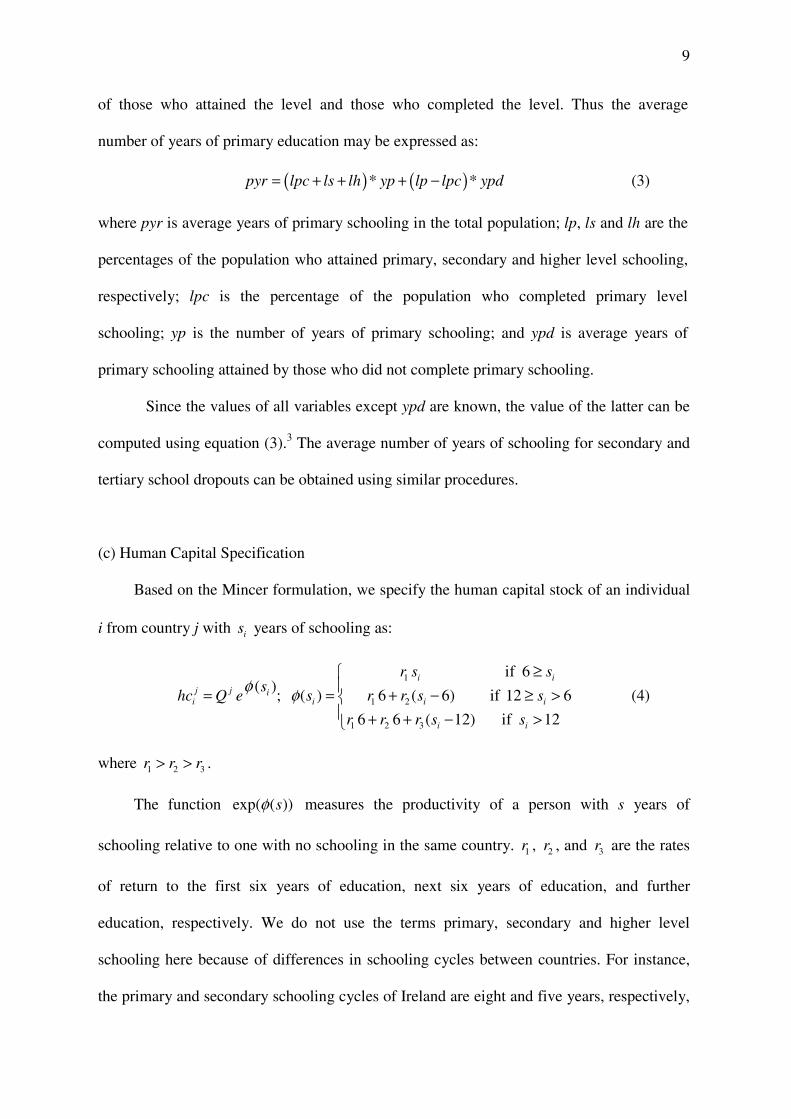
of those who attained the level and those who completed the level. Thus the average
number of years of primary education may be expressed as:
( ) ( )* *pyr lpc ls lh yp lp lpc ypd= + + + − (3)
where pyr is average years of primary schooling in the total population; lp, ls and lh are the
percentages of the population who attained primary, secondary and higher level schooling,
respectively; lpc is the percentage of the population who completed primary level
schooling; yp is the number of years of primary schooling; and ypd is average years of
primary schooling attained by those who did not complete primary schooling.
Since the values of all variables except ypd are known, the value of the latter can be
computed using equation (3).3 The average number of years of schooling for secondary and
tertiary school dropouts can be obtained using similar procedures.
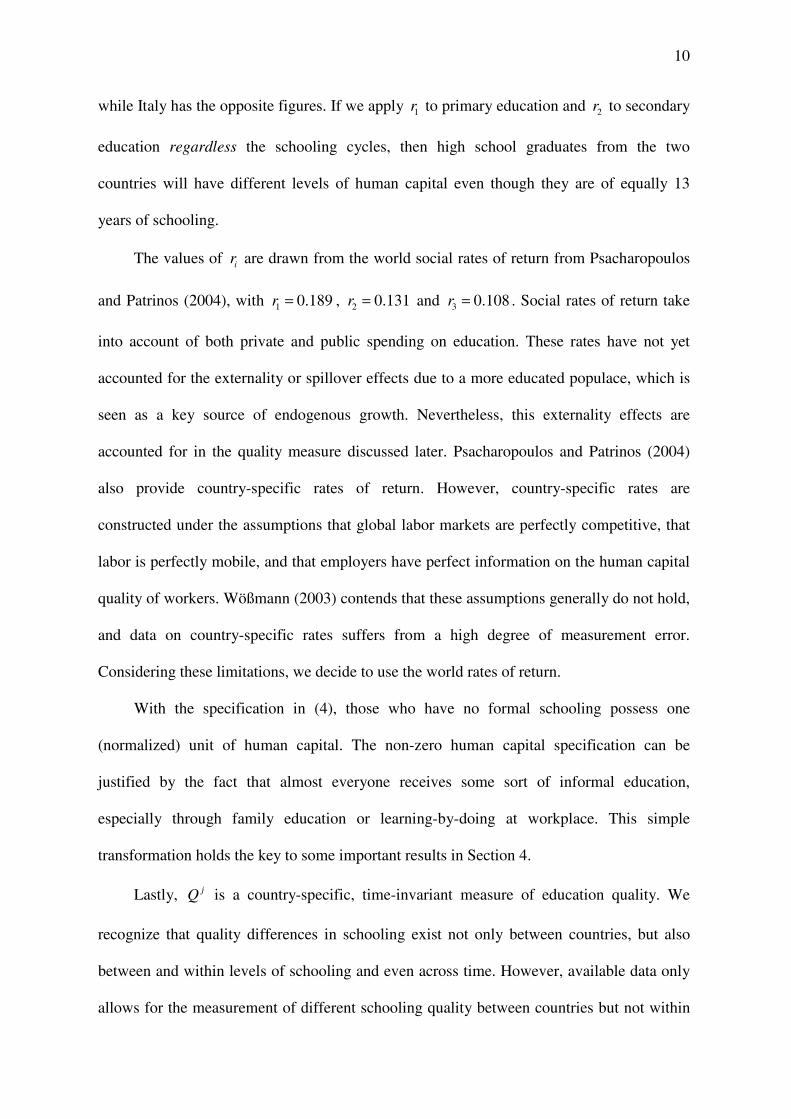
(c) Human Capital Specification
Based on the Mincer formulation, we specify the human capital stock of an individual
i from country j with is years of schooling as:
1
1 2
1 2 3
if 6( )
; ( ) 6 ( 6) if 12 6
6 6 ( 12) if 12
i i
j j ii i i i
i i
r s ss
hc Q e s r r s s
r r r s s
φ φ≥
= = + − ≥ > + + − >
(4)
where 1 2 3r r r> > .
The function exp( ( ))sφ measures the productivity of a person with s years of
schooling relative to one with no schooling in the same country. 1r , 2r , and 3r are the rates
of return to the first six years of education, next six years of education, and further
education, respectively. We do not use the terms primary, secondary and higher level
schooling here because of differences in schooling cycles between countries. For instance,
the primary and secondary schooling cycles of Ireland are eight and five years, respectively,
10
while Italy has the opposite figures. If we apply 1r to primary education and 2r to secondary
education regardless the schooling cycles, then high school graduates from the two
countries will have different levels of human capital even though they are of equally 13
years of schooling.
The values of ir are drawn from the world social rates of return from Psacharopoulos
and Patrinos (2004), with 1 0.189r = , 2 0.131r = and 3 0.108r = . Social rates of return take
into account of both private and public spending on education. These rates have not yet
accounted for the externality or spillover effects due to a more educated populace, which is
seen as a key source of endogenous growth. Nevertheless, this externality effects are
accounted for in the quality measure discussed later. Psacharopoulos and Patrinos (2004)
also provide country-specific rates of return. However, country-specific rates are
constructed under the assumptions that global labor markets are perfectly competitive, that
labor is perfectly mobile, and that employers have perfect information on the human capital
quality of workers. Wößmann (2003) contends that these assumptions generally do not hold,
and data on country-specific rates suffers from a high degree of measurement error.
Considering these limitations, we decide to use the world rates of return.
With the specification in (4), those who have no formal schooling possess one
(normalized) unit of human capital. The non-zero human capital specification can be
justified by the fact that almost everyone receives some sort of informal education,
especially through family education or learning-by-doing at workplace. This simple
transformation holds the key to some important results in Section 4.
Lastly, jQ is a country-specific, time-invariant measure of education quality. We
recognize that quality differences in schooling exist not only between countries, but also
between and within levels of schooling and even across time. However, available data only
allows for the measurement of different schooling quality between countries but not within
11
countries. Also, given the available data, we are unable to evaluate the differences in
education quality over time.4 Moreover, since jQ is uniformly applied to everyone within a
country, including those with no formal education, it means that we assume the relative
qualities of informal education between countries are the same as those of formal education.
This is partly to reflect the fact that formal education could spillover to informal education
and partly to simplify the specification. The values of jQ are largely drawn from Hanushek
and Kimko (2000) with minor extension. The construction of jQ is detailed in the appendix.
(d) Education and Human Capital Inequality
Different from previous studies that treat education and human capital inequalities
synonymously, we distinguish between the two concepts in the following analysis while
also seeking to establish the relationship between them. We measure the distribution of
education and human capital in the same way as how income distribution is measured. The
Gini coefficient is used as the main measure of education and human capital dispersion.
Alternative inequality measures such as standard deviation, coefficient of variation and
Theil index will also be computed and presented later.
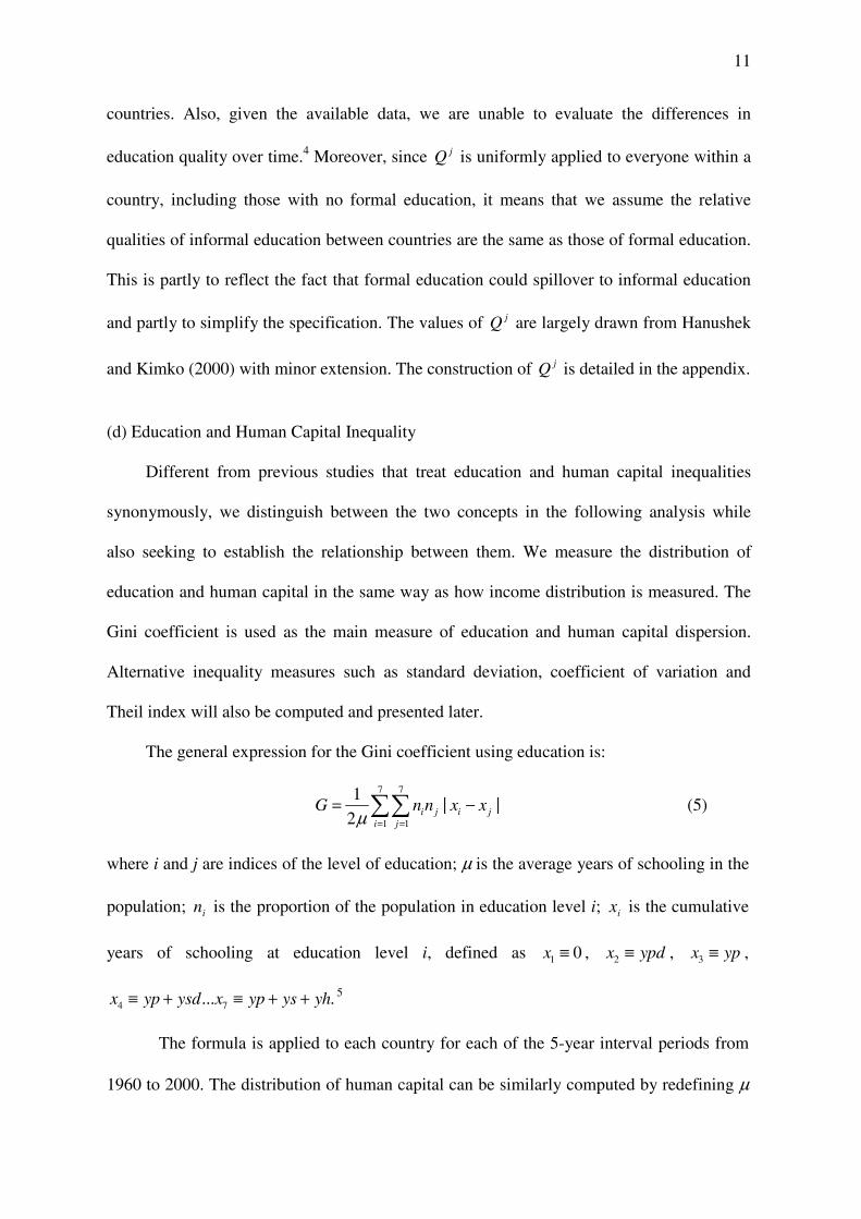
The general expression for the Gini coefficient using education is:
7 7
1 1
1| |
2 i j i ji j
G n n x xµ = =
= −∑∑ (5)
where i and j are indices of the level of education; µ is the average years of schooling in the
population; in is the proportion of the population in education level i; ix is the cumulative
years of schooling at education level i, defined as 1 0x ≡ , 2x ypd≡ , 3x yp≡ ,
4 7... .x yp ysd x yp ys yh≡ + ≡ + + 5
The formula is applied to each country for each of the 5-year interval periods from
1960 to 2000. The distribution of human capital can be similarly computed by redefining µ
12
to be the average human capital in the population, and ix to be the amount of human capital
cumulated through schooling up to education level i as specified in (4).
4. EMPIRICAL RESULTS
(a) Average Education and Average Human Capital
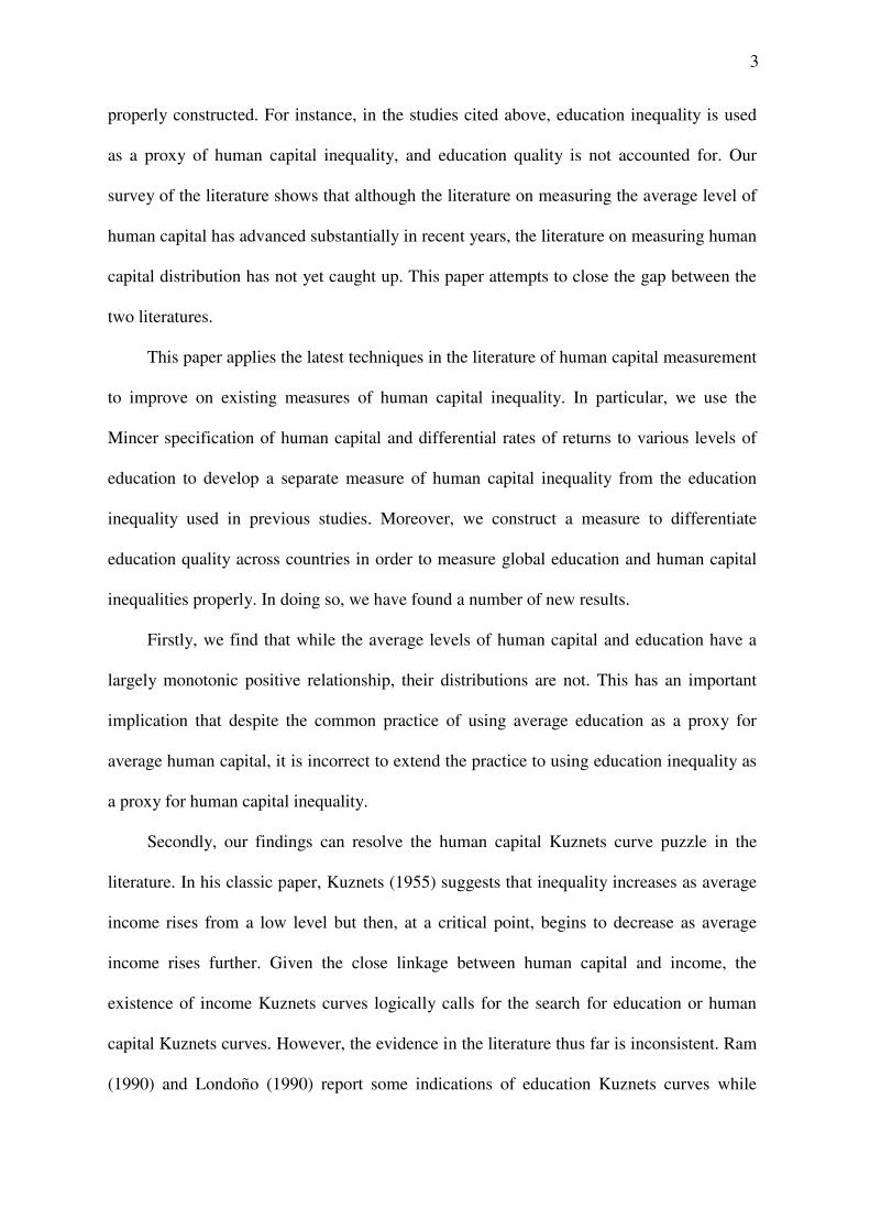
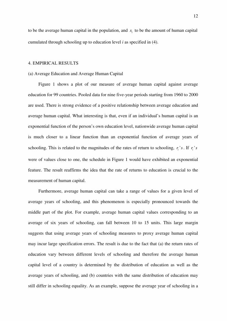
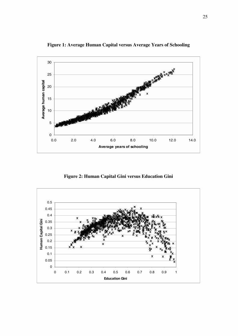
Figure 1 shows a plot of our measure of average human capital against average
education for 99 countries. Pooled data for nine five-year periods starting from 1960 to 2000
are used. There is strong evidence of a positive relationship between average education and
average human capital. What interesting is that, even if an individual�s human capital is an
exponential function of the person�s own education level, nationwide average human capital
is much closer to a linear function than an exponential function of average years of
schooling. This is related to the magnitudes of the rates of return to schooling, 'ir s . If 'ir s
were of values close to one, the schedule in Figure 1 would have exhibited an exponential
feature. The result reaffirms the idea that the rate of returns to education is crucial to the
measurement of human capital.
Furthermore, average human capital can take a range of values for a given level of
average years of schooling, and this phenomenon is especially pronounced towards the
middle part of the plot. For example, average human capital values corresponding to an
average of six years of schooling, can fall between 10 to 15 units. This large margin
suggests that using average years of schooling measures to proxy average human capital
may incur large specification errors. The result is due to the fact that (a) the return rates of
education vary between different levels of schooling and therefore the average human
capital level of a country is determined by the distribution of education as well as the
average years of schooling, and (b) countries with the same distribution of education may
still differ in schooling equality. As an example, suppose the average year of schooling in a
13
community of 16 people is equal to one, i.e. total years of schooling are equal to 16. The
average human capital of the community will be 30 percent higher if all 16 years of
schooling are acquired by a single person (i.e. prefect inequality) compared to the case that
two persons have eight years of schooling. However, if everyone has one year of schooling
(i.e. prefect equality) then average human capital is 84 percent higher than the case of
prefect inequality.
(Figure 1 here)
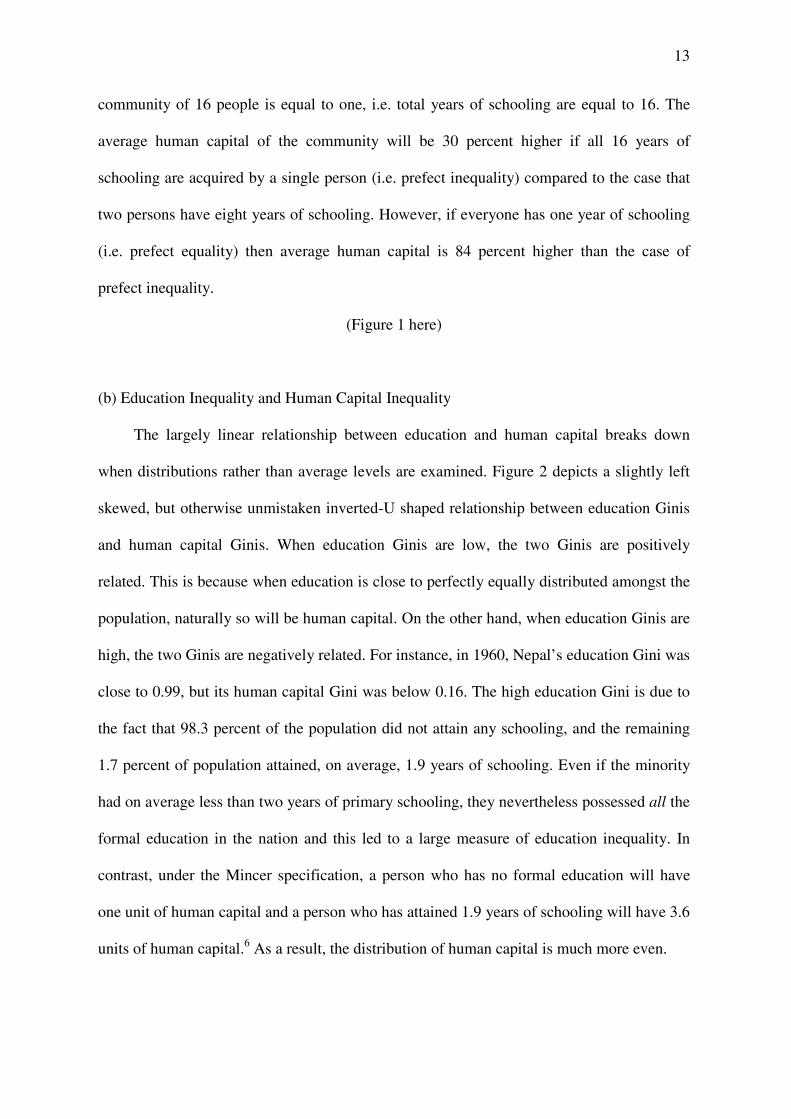
(b) Education Inequality and Human Capital Inequality
The largely linear relationship between education and human capital breaks down
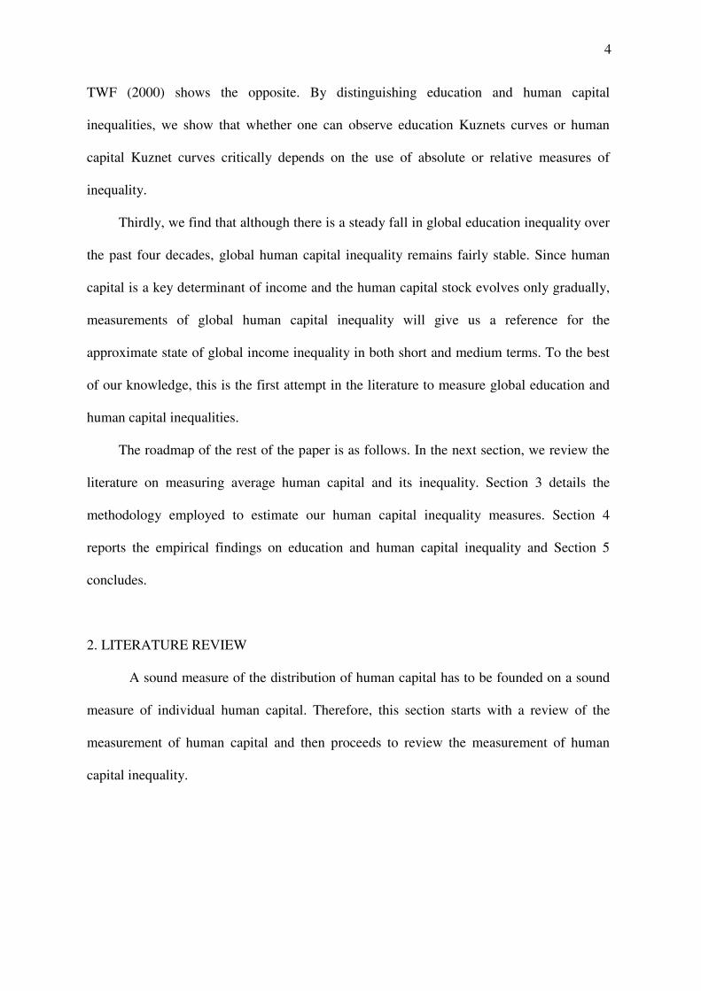
when distributions rather than average levels are examined. Figure 2 depicts a slightly left
skewed, but otherwise unmistaken inverted-U shaped relationship between education Ginis
and human capital Ginis. When education Ginis are low, the two Ginis are positively
related. This is because when education is close to perfectly equally distributed amongst the
population, naturally so will be human capital. On the other hand, when education Ginis are
high, the two Ginis are negatively related. For instance, in 1960, Nepal�s education Gini was
close to 0.99, but its human capital Gini was below 0.16. The high education Gini is due to
the fact that 98.3 percent of the population did not attain any schooling, and the remaining
1.7 percent of population attained, on average, 1.9 years of schooling. Even if the minority
had on average less than two years of primary schooling, they nevertheless possessed all the
formal education in the nation and this led to a large measure of education inequality. In
contrast, under the Mincer specification, a person who has no formal education will have
one unit of human capital and a person who has attained 1.9 years of schooling will have 3.6
units of human capital.6 As a result, the distribution of human capital is much more even.
14
The Nepalese example clearly illustrates that using formal education as a proxy of
human capital is particularly problematic when average years of schooling are low, because
in such a situation informal education will constitute a significant part of human capital. The
Mincer specification in equation (4) provides a simple means to acknowledge those
immeasurable components of human capital.
Furthermore, the points in Figure 2 are closely clustered towards the left hand side.
This is expected because if education is perfectly equally distributed, human capital should
also be perfectly equally distributed, after excluding individual ability and experience.
However, the points are increasingly dispersed as they move towards the right. This is,
again, because of the changing return rates to education with the level of schooling.
(Figure 2 here)
An important implication of Figures 1 and 2 is that, whereas using average education
as a proxy of average human capital incurs some measurement errors, using education
inequality as a proxy of human capital inequality is conceptually misleading.
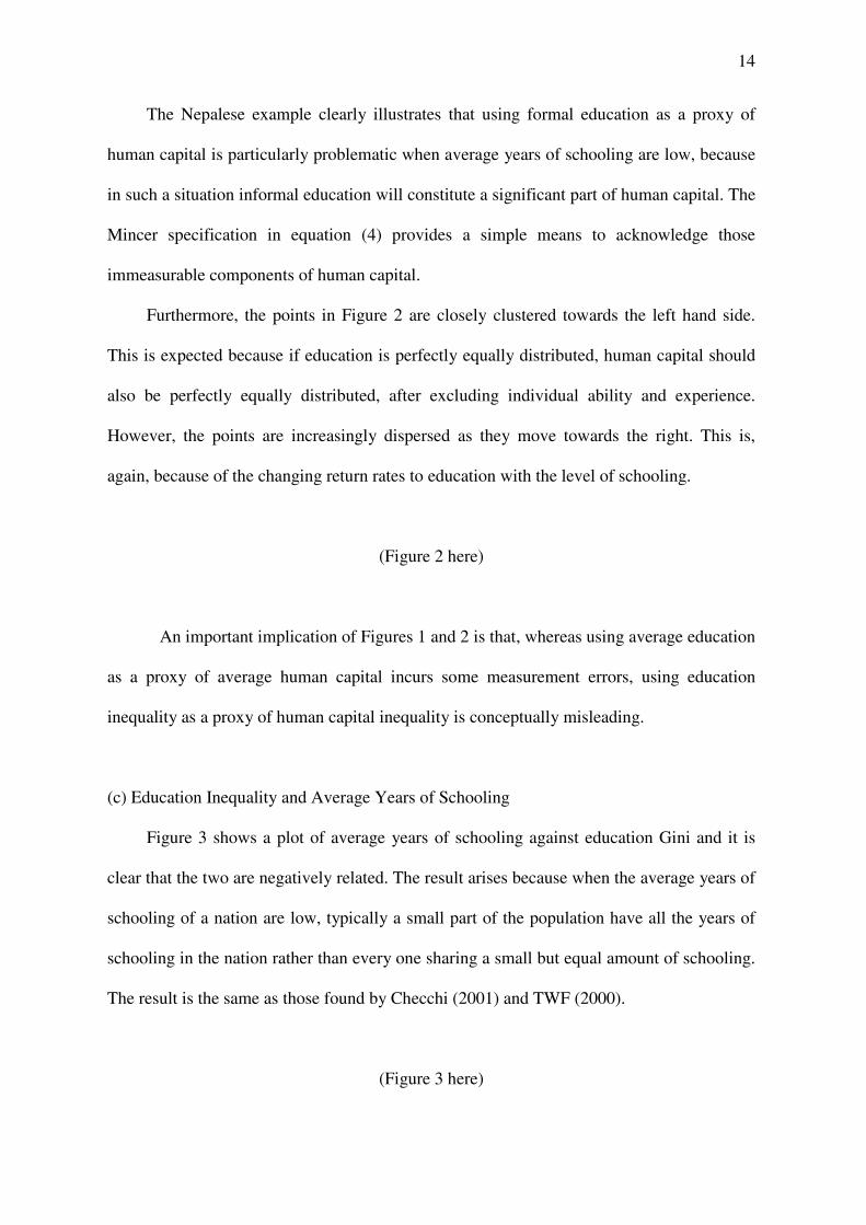
(c) Education Inequality and Average Years of Schooling
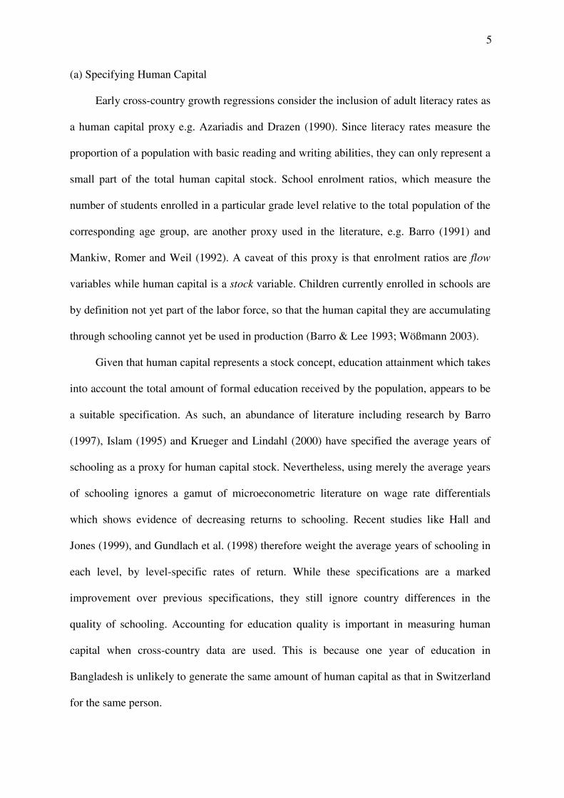
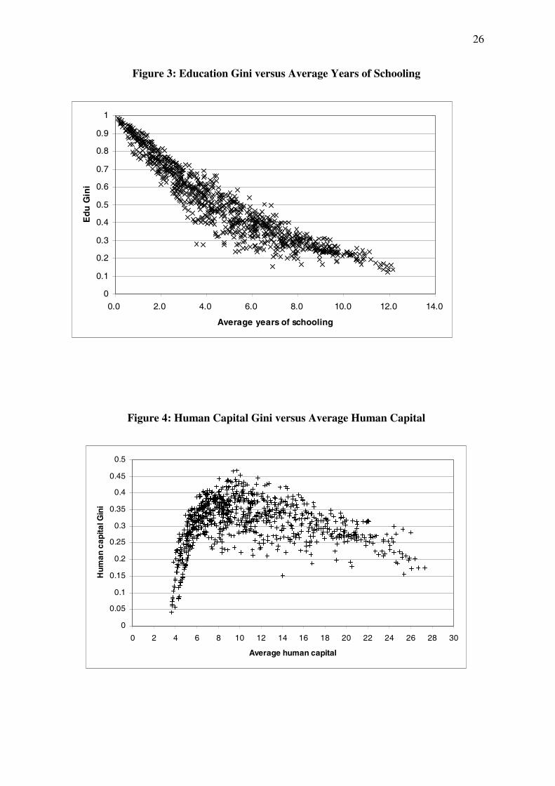
Figure 3 shows a plot of average years of schooling against education Gini and it is
clear that the two are negatively related. The result arises because when the average years of
schooling of a nation are low, typically a small part of the population have all the years of
schooling in the nation rather than every one sharing a small but equal amount of schooling.
The result is the same as those found by Checchi (2001) and TWF (2000).
(Figure 3 here)
15
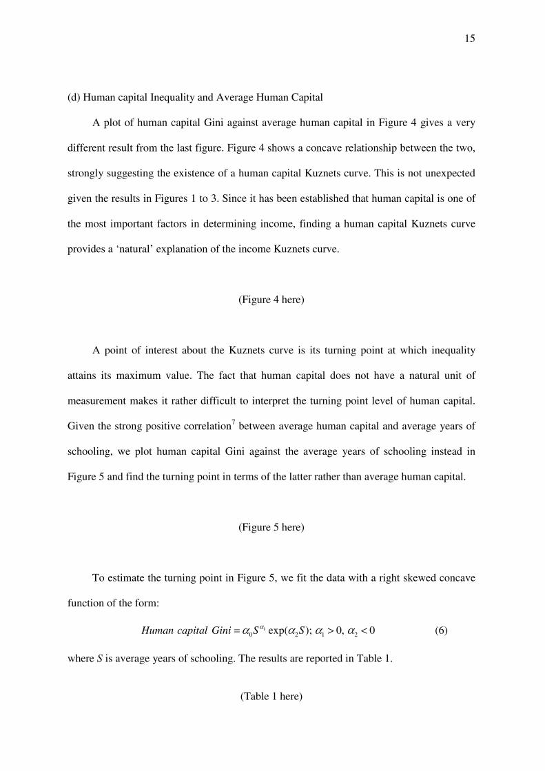
(d) Human capital Inequality and Average Human Capital
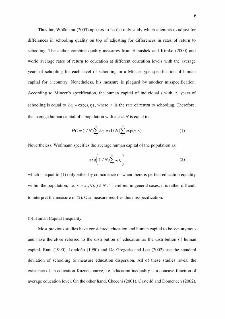
A plot of human capital Gini against average human capital in Figure 4 gives a very
different result from the last figure. Figure 4 shows a concave relationship between the two,
strongly suggesting the existence of a human capital Kuznets curve. This is not unexpected
given the results in Figures 1 to 3. Since it has been established that human capital is one of
the most important factors in determining income, finding a human capital Kuznets curve
provides a �natural� explanation of the income Kuznets curve.
(Figure 4 here)
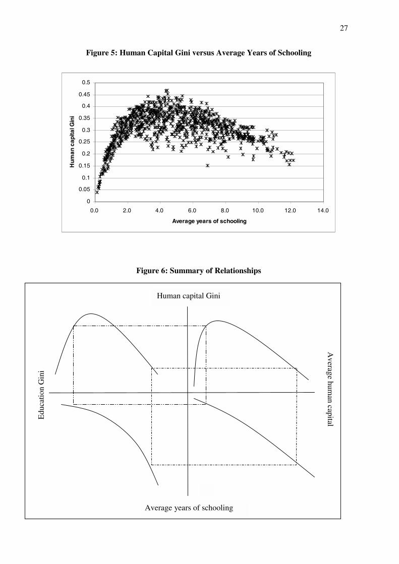
A point of interest about the Kuznets curve is its turning point at which inequality
attains its maximum value. The fact that human capital does not have a natural unit of
measurement makes it rather difficult to interpret the turning point level of human capital.
Given the strong positive correlation7 between average human capital and average years of
schooling, we plot human capital Gini against the average years of schooling instead in
Figure 5 and find the turning point in terms of the latter rather than average human capital.
(Figure 5 here)
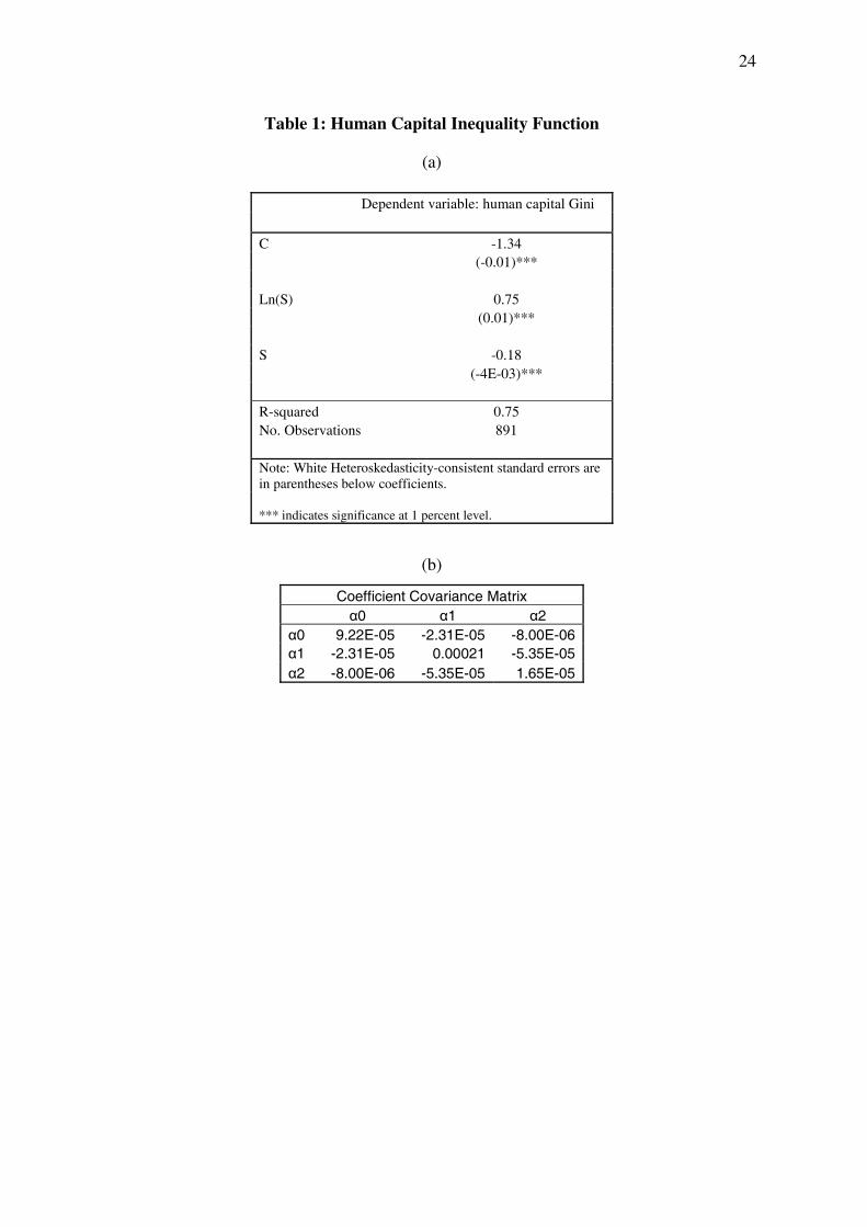
To estimate the turning point in Figure 5, we fit the data with a right skewed concave
function of the form:
10 2 1 2exp( ); 0, 0Human capital Gini S Sαα α α α= > < (6)
where S is average years of schooling. The results are reported in Table 1.
(Table 1 here)
16
The turning point of (6) occurs when S equals to 1 2α α− . Using Theorem 4 of Mood
et al (1974, p. 181),8 the expected value of 1 2α α− is estimated to be 4.165 years and its
variance to be 0.0016. Given the small variance, the point estimate is highly accurate for our
dataset. Moreover, this estimated figure of average years of schooling ties closely with that
calculated by De Gregorio and Lee (2002). The corresponding human capital Gini at the
turning point is 0.36.
By 2000, a substantial number of Sub-Saharan African countries still have average
years of schooling well below 4.2; for example, Mali (0.76), Niger (0.82), Mozambique
(1.2), Gambia (1.9), Rwanda (2.0), Sierra Leone (2.0), and Liberia (2.3). In other regions,
there are also many low income countries being far away from passing the turning point
level of average education, for instance, Afghanistan (1.1), Nepal (1.9), Papua New Guinea
(2.4), Pakistan (2.5), Bangladesh (2.5), Haiti (2.7), and Guatemala (3.1).
The evidence of a human capital Kuznets curve and the position of its turning point
have important implications for education policy, such as the United Nations� second
Millennium Development Goal (MDG). The second MDG is to ensure that by 2015,
children everywhere, boys and girls alike, will be able to complete a full course of primary
schooling. If the UN successfully achieves its target, we should then observe average years
of schooling in the least developing countries to increase. However, if a nation�s starting
average years of schooling is well below the threshold level of 4.2, one may observe human
capital inequality, and thus possibly income inequality, to increase rather than to decrease as
the nation achieves universal primary education. Furthermore, due to the fact that part of the
adult population may have little or zero formal schooling, even if universal primary
education is achieved by 2015, the average years of schooling for the workforce may remain
below the threshold level for many years to come. Therefore, policymakers should be
17
cautious in expecting falling income inequality in the society as an incentive of
accomplishing the MDG. Nevertheless, it is equally unwarranted to advocate that, if a
nation falls below the 4.2 year threshold level, an educational expansion will definitely be
accomplished with raising inequality. For example, expenditure inequality may not link to
income inequality if there is resource sharing within households. In particular, households
with uneducated parents could still benefit if their children can receive education and earn
higher incomes in the future than the parents themselves could have. To put all these
arguments into perspective, it is useful to refer to the findings of a recent survey by Hannum
& Buchmann (2004) on the impact on socio-economic development of educational
expansion. The survey finds that decades of sociological studies give no evidence that
educational expansion necessarily reduces socio-economic inequality.
As a way to conclude this section, we summarize the inter-relationships between the
level and distribution of education and human capital using a simple four-quadrant diagram
in Figure 6.
(Figure 6 here)
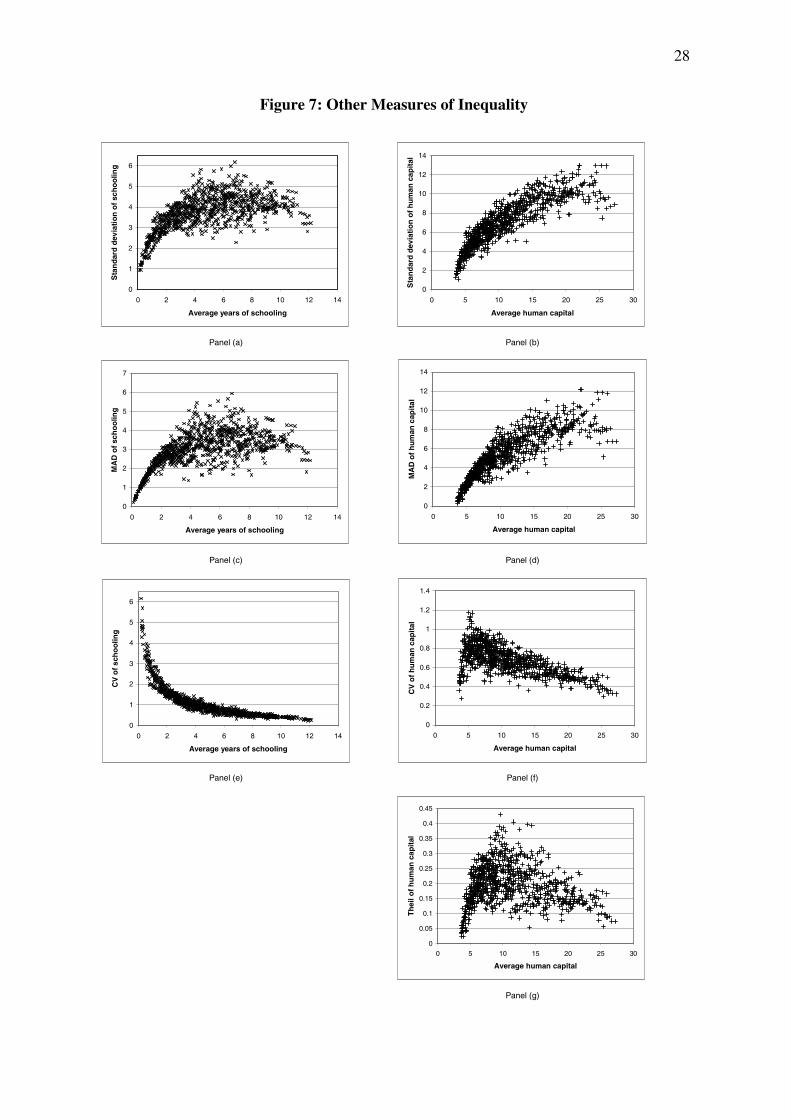
(e) Other Measures of Inequality
The discussion on inequality so far is based on a relative measurement of inequality �
the Gini coefficient. Nevertheless, there is an array of inequality measures, ranging from
other relative measures like the Theil entropy measure and the coefficient of variation (CV),
to absolute measures like the standard deviation (SD) and the mean absolute deviation
(MAD). Since policymakers may use multiple measures of inequality, it is important to
know how robust the human capital Kuznets curve is with respect to different measures of
inequality. Figure 7 shows how the use of other inequality measures alters the results in
18
Figures 3 and 4, respectively. Theil measure is not calculated for education inequality
because it is undefined when a portion of the population has zero year of schooling.
(Figure 7 here)
In Figure 7, we observe an education Kuznets curve when SD and MAD are used but
not when CV is used. Londoño (1990), Ram (1990), De Gregorio and Lee (2002) and TWF
(2002) find similar education Kuznets curves using SD as an inequality measure. In
addition, we observe a clear human capital Kuznets curve when Theil and CV are used.
When SD and MAD are used, although human capital inequality and average human capital
display a slightly concave relationship, there are insufficient observations on the far right of
panels (b) and (d) to confirm a Kuznets curve. In general, the human capital Kuznets curves
in panels (f) and (g) as well as in Figure 3 appear to be much more pronounced than the
education Kuznets curves in panels (a) and (c).
The fact that we cannot observe education Kuznets curves when using relative
measures of inequality is not by chance. Relative measures of education inequality are
essentially some absolute measures of education inequality divided by average years of
schooling. When average years of schooling tend to zero, even if absolute measures of
education inequality are small, relative measures of education inequality will tend to the
upper bound (i.e. 1 for Gini coefficient and infinity for CV), resulting in a downward
sloping relationship between relative measures of education inequality and average years of
schooling. In the case of human capital, due to the Mincer specification, average human
capital is bound to be bigger than one and therefore prevents the relative measures of human
capital inequality from reaching their upper bound values. Our findings thus not only
highlight the sensitivity of education and human capital to different measures of inequality
19
but also explain why there is inconsistent evidence between education and human capital
Kuznet curves in the literature.
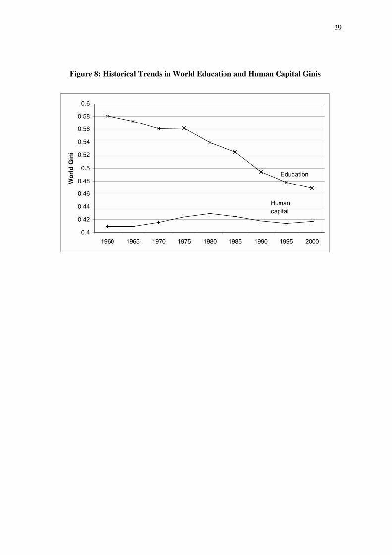
(f) World Education and Human Capital Inequality
Since the dataset covers at least 84 percent of the world population, it can be used to
construct a measure of world education and human capital inequality. Country population
size is accounted for in constructing these inequality measures. The result is shown in
Figure 8. Recall that country-specific measures of education quality are static over time;
thus, the changes in world human capital inequality are due largely to changes in the
quantity of education (its total and distribution) amongst nations over time.
(Figure 8 here)
Over the 40 year period, there has been a steady decrease in education Ginis across the
world and the pace of it has increased since 1975. Average years of schooling for the world,
as expected, has also increased steadily during the period from 3.5 years in 1960 to 6.3 years
in 2000. On the contrary, the world human capital Gini exhibits a slightly concave trend
with a peak at about 0.43 Gini points in 1980. Therefore, the inter-relationships between the
world education and human capital resemble those described in the four-quadrant diagram
in Figure 6. Furthermore, the evolution path of the world�s human capital stock resembles a
Kuznets curve, and it reaches the turning point in 1980. In that year, the world average years
of schooling are equal to 4.4, which is very close to the previously estimated 4.2 years using
national data.
20
5. CONCLUSION
One of the issues confounding modern growth economists is the search for a suitable
proxy for human capital. A substantial part of the empirical literature in growth has been
devoted to attempting to quantify the contribution of human capital, particularly the capital
derived from investments in education. After the initial explosion of literature discussing the
average quantity of human capital, recent research has begun to focus on the importance of
the distribution of human capital in affecting growth. However, the measurement of human
capital distribution has lagged far behind that of the average level of human capital. The
mis-measurement of human capital distribution will lead to errors in empirical research and
may adversely affect policy makers� decisions. Hence, the main objective of this paper was
to improve on existing measures of human capital distribution. Our improved measure was
then applied in an analysis of education and human capital inequalities, on both national and
global scales.
Our findings highlighted the importance in distinguishing between education and
human capital. Although average education and average human capital exhibited a strong
positive correlation, the use of average education to proxy for human capital is subject to a
large margin of error. It was also found that the relationship between education and human
capital inequality measured by Gini coefficients was concave, implying that using education
inequality as a proxy of human capital inequality could lead to completely misleading
findings. Furthermore, there was clear evidence of a human capital Kuznets curve with a
turning point at about 4.2 years of schooling. This result had particular implications for
policymakers in that promoting universal primary education as set out in the UN�s second
MDG, may lead to an increase rather than a decrease in human capital inequality.
Policymakers should be cautious in expecting a fall in income gap in the society as a
consequence of their education campaigns.
21
The evidence of a human capital Kuznets curve provided a natural explanation for the
occurrence of the income Kuznets curve. However, the human capital Kuznets was only
observed when we used relative measures of inequality. On the contrary, an education
Kuznets curve was observed only when absolute measures of inequality were used, such as
the coefficient of variation. These findings thus explained why there was inconsistent
evidence in the literature about the existence of education or human capital Kuznets curves
when different inequality measures were used.
On a global scale, human capital Ginis have remained rather static throughout the past
four decades even though education Ginis trended downwards. It is interesting to read this
result along side with that of Dowrick & Akmal (2005). The study finds that global income
inequality, when measured by a Gini coefficient using �true Afriat income,� was largely
stable over the 1980s and the 1990s.
As mentioned in previous sections, a limitation of the human capital measure
constructed in the literature is the lack of reliable measures of education quality that can
account for quality inequality between countries and within countries, at a point in time and
over time. This is likely to be a very fruitful (but data demanding) research area. Lastly, as
labor and education markets are increasingly globalized, the flows of foreign and migrant
workers and international students will be increasingly important in defining the human
capital content of the labor force of a country. Another item on the research agenda,
therefore, is how to account for these global flows of human capital in the construction of a
national human capital stock.
22
REFERENCES
Azariadis, C & Drazen, A 1990, 'Threshold Externalities in Economic Development', Quarterly Journal of Economics, vol. 105, no. 2, pp. 501-26.
Baker, M & Benjamin, D 1994, 'The performance of immigrants in the Canadian labor market', Journal of Labor Economics, vol. 12, no. 3, pp. 369-405.
Barro, RJ 1997, Determinants of Economic Growth: A Cross-Country Empirical Study, MIT Press, Cambridge, Massachusetts.
---- 2001, 'Human Capital and Growth', The American Economic Review, vol. 91, no. 2, pp. 12-7.
Barro, RJ & Lee, J-W 1993, 'International Comparisons of Educational Attainment', Journal of Monetary Economics, vol. 32, pp. 363 - 94.
---- 2000, International Data on Educational Attainment: Updates and Implications, Working Paper No. 7911, National Bureau of Economic Research.
Castelló, A & Doménech, R 2002, 'Human Capital Inequality and Economic Growth: Some New Evidence', The Economic Journal, vol. 112, pp. 187 - 200.
Checchi, D 2001, 'Education, Inequality and Income Inequality', Distributional Analysis Research Programme, no. DARP 52.
De Gregorio, J & Lee, J-W 2002, 'Education and Income Inequality: New Evidence from Cross-country Data', Review of Income and Wealth, vol. 48, no. 3, pp. 395-416.
Dowrick, S & Akmal, M 2005, 'Contradictory Trends in Global Income Inequality: A Tale of Two Biases', Review of Income and Wealth, vol. 51, no. 2, pp. 201-29.
Gundlach, E, Rudman, D & Wößmann, L 1998, 'Second Thoughts on Development Accounting', Kiel Working Paper, no. 895. Hall, RE & Jones, CI 1999, 'Why Do Some Countries Produce So Much More Output per Worker Than Others?' Quarterly Journal of Economics, vol. 114, no. 1,
pp. 83-116. Hannum, E & Buchmann, C 2004, 'Global educational expansion and socio-economic
development: an assessment of findings from the social sciences', World Development, vol. 33, no. 3, pp. 333-54.
Hanushek, EA & Kimko, DD 2000, 'Schooling, Labor-Force Quality, and the Growth of Nations', The American Economic Review, vol. 90, no. 5, pp. 1184-208.
Islam, N 1995, 'Growth Empirics: A Panel Data Approach', The Quarterly Journal of Economics, vol. 110, no. 4, pp. 1127-70.
Kee, P 1995, 'Native-immigrant wage differentials in the Netherlands: discrimination?' Oxford Economic Papers, vol. 47, no. 2, pp. 302-17.
Krueger, A & Lindahl, M 2000, Education for Growth: Why and For Whom?, Working Paper No. 7591, National Bureau of Economic Research.
Kuznets, S 1955, 'Economic Growth and Income Inequality', American Economic Review, vol. 45, no. 1, pp. 1-28.
Londoño, JL 1990, 'Kuznetsian Tales with Attention to Human Capital', paper presented to Third Inter-American Seminar in Economics, Rio de Janeiro, Brazil.
Mankiw, NG, Romer, D & Weil, DN 1992, 'A Contribution to the Empirics of Economic Growth', The Quarterly Journal of Economics, vol. 107, no. 2, pp. 407-37.
Mincer, J 1974, Schooling, Experience, And Earnings, National Bureau of Economic Research, New York and London.
Mood, AM, Graybill, FA & Boes, DC 1974, Introduction to the Theory of Statistics, 3rd edn, McGraw-Hill, Tokyo.
Psacharopoulos, G & Arriagada, A-M 1986, The Educational Attainment of the Labor Force: An International Comparison, EDT38, The World Bank.
23
Psacharopoulos, G & Patrinos, HA 2004, 'Returns to Investment in Education: A Further Update', Education Economics, vol. 12, no. 2, pp. 111 - 34.
Ram, R 1990, 'Educational Expansion and Schooling Inequality; International Evidence and Some Implications', The Review of Economics and Statistics, vol. 72, no. 2, pp. 266-74.
Thomas, V, Wang, Y & Fan, X 2000, 'Measuring Education Inequality: Gini Coefficients of Education', World Bank Policy Research Working Paper, no. WPS2525.
---- 2002, A New Dataset on Inequality in Education: Gini and Theil Indices of Schooling for 140 Countries, 1960 - 2000, The World Bank, Washington.
Wößmann, L 2003, 'Specifying Human Capital', Journal of Economic Surveys, vol. 17, no. 3, pp. 239-70.
24
Table 1: Human Capital Inequality Function
(a)
Dependent variable: human capital Gini
C -1.34 (-0.01)*** Ln(S) 0.75 (0.01)*** S -0.18 (-4E-03)***
R-squared 0.75 No. Observations 891 Note: White Heteroskedasticity-consistent standard errors are in parentheses below coefficients. *** indicates significance at 1 percent level.
(b)
Coefficient Covariance Matrix α0 α1 α2 α0 9.22E-05 -2.31E-05 -8.00E-06 α1 -2.31E-05 0.00021 -5.35E-05 α2 -8.00E-06 -5.35E-05 1.65E-05
25
Figure 1: Average Human Capital versus Average Years of Schooling
0
5
10
15
20
25
30
0.0 2.0 4.0 6.0 8.0 10.0 12.0 14.0
Average years of schooling
Ave
rag
e h
um
an c
apit
al
Figure 2: Human Capital Gini versus Education Gini
0
0.05
0.1
0.15
0.2
0.25
0.3
0.35
0.4
0.45
0.5
0 0.1 0.2 0.3 0.4 0.5 0.6 0.7 0.8 0.9 1
Education Gini
Hum
an C
apita
l Gin
i
26
Figure 3: Education Gini versus Average Years of Schooling
0
0.1
0.2
0.3
0.4
0.5
0.6
0.7
0.8
0.9
1
0.0 2.0 4.0 6.0 8.0 10.0 12.0 14.0
Average years of schooling
Ed
u G
ini
Figure 4: Human Capital Gini versus Average Human Capital
0
0.05
0.1
0.15
0.2
0.25
0.3
0.35
0.4
0.45
0.5
0 2 4 6 8 10 12 14 16 18 20 22 24 26 28 30
Average human capital
Hum
an c
apita
l Gin
i
27
Figure 5: Human Capital Gini versus Average Years of Schooling
0
0.05
0.1
0.15
0.2
0.25
0.3
0.35
0.4
0.45
0.5
0.0 2.0 4.0 6.0 8.0 10.0 12.0 14.0
Average years of schooling
Hum
an c
apita
l Gin
i
Figure 6: Summary of Relationships
Human capital Gini
Average years of schooling
Average hum
an capital
Edu
catio
n G
ini
28
Figure 7: Other Measures of Inequality
Panel (f)Panel (e)
Panel (g)
Panel (b)Panel (a)
Panel (c) Panel (d)
0
1
2
3
4
5
6
0 2 4 6 8 10 12 14
Average years of schooling
Sta
nd
ard
dev
iati
on
of
sch
oo
ling
0
2
4
6
8
10
12
14
0 5 10 15 20 25 30
Average human capital
Sta
nd
ard
dev
iati
on
of
hu
man
cap
ital
0
1
2
3
4
5
6
0 2 4 6 8 10 12 14
Average years of schooling
CV
of
sch
oo
ling
0
0.2
0.4
0.6
0.8
1
1.2
1.4
0 5 10 15 20 25 30
Average human capital
CV
of
hu
man
cap
ital
0
1
2
3
4
5
6
7
0 2 4 6 8 10 12 14
Average years of schooling
MA
D o
f sc
ho
olin
g
0
2
4
6
8
10
12
14
0 5 10 15 20 25 30
Average human capital
MA
D o
f h
um
an c
apit
al
0
0.05
0.1
0.15
0.2
0.25
0.3
0.35
0.4
0.45
0 5 10 15 20 25 30
Average human capital
Th
eil o
f h
um
an c
apit
al
29
Figure 8: Historical Trends in World Education and Human Capital Ginis
0.4
0.42
0.44
0.46
0.48
0.5
0.52
0.54
0.56
0.58
0.6
1960 1965 1970 1975 1980 1985 1990 1995 2000
Wo
rld
Gin
i
Education
Human capital
30
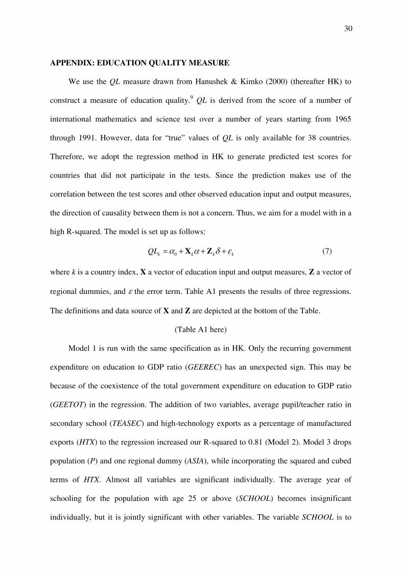
APPENDIX: EDUCATION QUALITY MEASURE
We use the QL measure drawn from Hanushek & Kimko (2000) (thereafter HK) to
construct a measure of education quality.9 QL is derived from the score of a number of
international mathematics and science test over a number of years starting from 1965
through 1991. However, data for �true� values of QL is only available for 38 countries.
Therefore, we adopt the regression method in HK to generate predicted test scores for
countries that did not participate in the tests. Since the prediction makes use of the
correlation between the test scores and other observed education input and output measures,
the direction of causality between them is not a concern. Thus, we aim for a model with in a
high R-squared. The model is set up as follows:
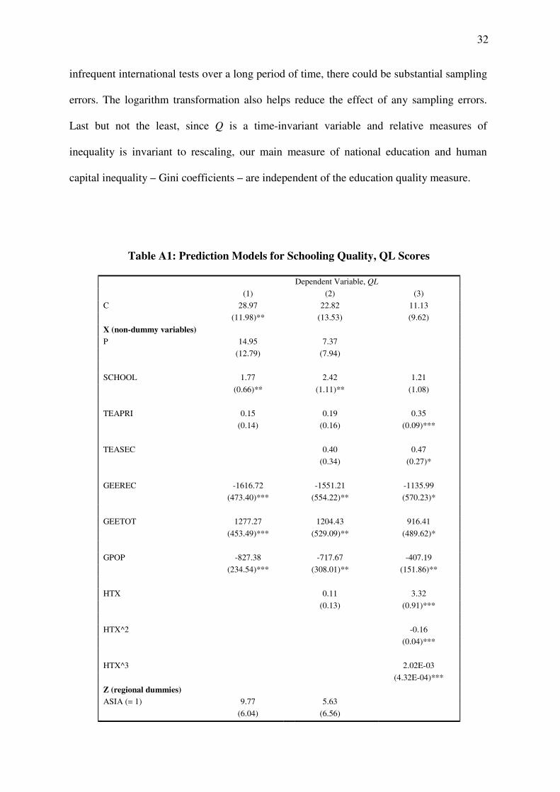
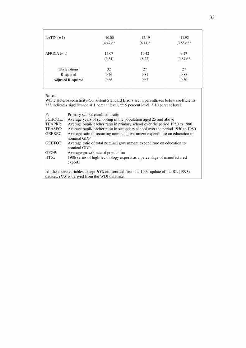
0k k k kQL α α δ ε= + + +X Z (7)
where k is a country index, X a vector of education input and output measures, Z a vector of
regional dummies, and ε the error term. Table A1 presents the results of three regressions.
The definitions and data source of X and Z are depicted at the bottom of the Table.
(Table A1 here)
Model 1 is run with the same specification as in HK. Only the recurring government
expenditure on education to GDP ratio (GEEREC) has an unexpected sign. This may be
because of the coexistence of the total government expenditure on education to GDP ratio
(GEETOT) in the regression. The addition of two variables, average pupil/teacher ratio in
secondary school (TEASEC) and high-technology exports as a percentage of manufactured
exports (HTX) to the regression increased our R-squared to 0.81 (Model 2). Model 3 drops
population (P) and one regional dummy (ASIA), while incorporating the squared and cubed
terms of HTX. Almost all variables are significant individually. The average year of
schooling for the population with age 25 or above (SCHOOL) becomes insignificant
individually, but it is jointly significant with other variables. The variable SCHOOL is to
31
account for the potential externality of individuals� education on the population�s human
capital stock. This externality effect of human capital accumulation is important in many
endogenous growth models. A Ramsey RESET test does not reject the null hypothesis that
Model 3 is of correct specification. Model 3 is also the one with the highest R-squared of
0.88, which makes it a suitable model for prediction purposes. Thus, Model 3 is chosen as
our preferred model.
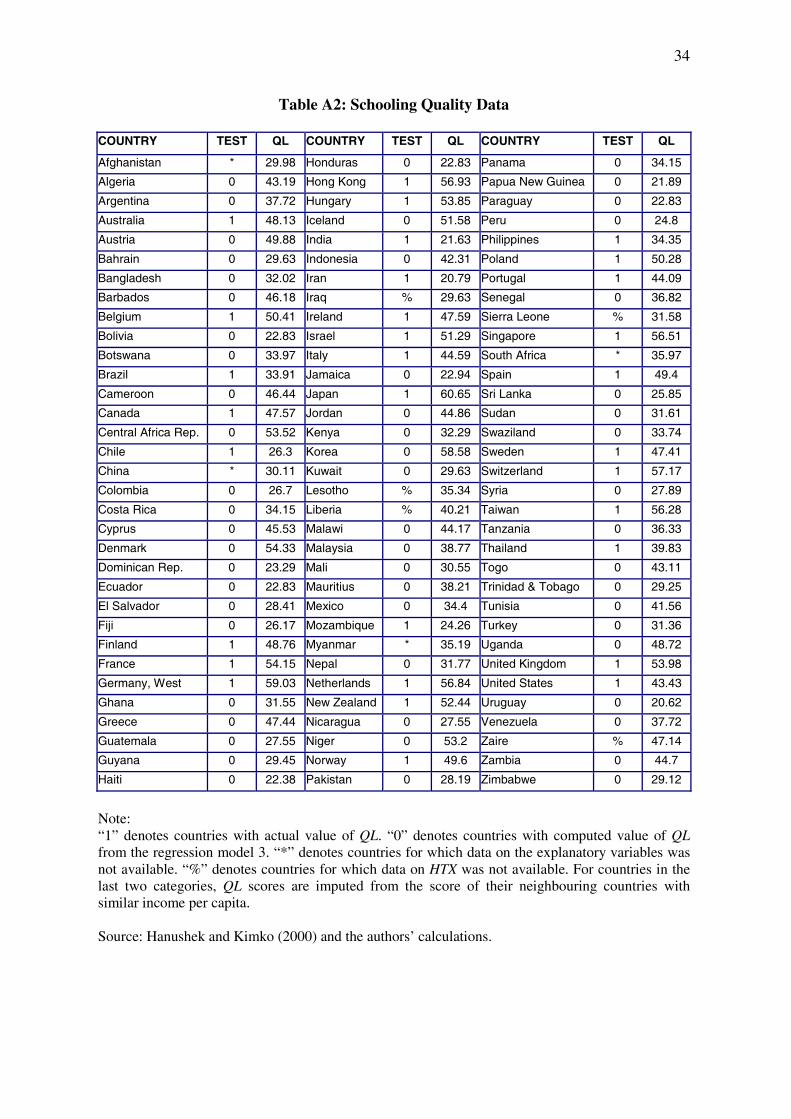
The actual observations of QL range between 20 and 60. Some of the predicted values
however fall out of these bounds and their accuracy could be a concern. For those countries,
we use the average scores of two countries in the same region; one with a GDP per capita
higher than the country in concern, and another with a lower per capita GDP. In doing so,
we assume that countries in the same region with similar per capita income have similar
spending behavior on education. The predicted and actual QL scores are shown in Table
A2.
The quality measure, Q, is defined as ln( )Q QL= . A logarithmic transformation is
used for two reasons. Firstly, directly applying the raw QL scores as Q in the human capital
specification implies that a student from developed countries would have human capital two
to three times that of a student from developing countries with the same years of schooling
(e.g. Japan and Uruguay), and the difference between developed countries would also be
over 20 percent (e.g. Japan and Finland). However, the literature on wage differentials
between migrant workers from less developed countries and native workers in developed
countries are of a order of magnitude between 10 to 50 percent only (Baker & Benjamin
1994; Kee 1995). Since migrant workers may face labor market discrimination, differences
in labor quality will account for an even smaller portion of the observed wage differentials.
The logarithmic function serves to bring the test scores differences between countries in line
with the evidence on wage differences. Secondly, since QL scores come from very
32
infrequent international tests over a long period of time, there could be substantial sampling
errors. The logarithm transformation also helps reduce the effect of any sampling errors.
Last but not the least, since Q is a time-invariant variable and relative measures of
inequality is invariant to rescaling, our main measure of national education and human
capital inequality � Gini coefficients � are independent of the education quality measure.
Table A1: Prediction Models for Schooling Quality, QL Scores
Dependent Variable, QL
(1) (2) (3)
C 28.97 22.82 11.13
(11.98)** (13.53) (9.62)
X (non-dummy variables)
P 14.95 7.37
(12.79) (7.94)
SCHOOL 1.77 2.42 1.21
(0.66)** (1.11)** (1.08)
TEAPRI 0.15 0.19 0.35
(0.14) (0.16) (0.09)***
TEASEC 0.40 0.47
(0.34) (0.27)*
GEEREC -1616.72 -1551.21 -1135.99
(473.40)*** (554.22)** (570.23)*
GEETOT 1277.27 1204.43 916.41
(453.49)*** (529.09)** (489.62)*
GPOP -827.38 -717.67 -407.19
(234.54)*** (308.01)** (151.86)**
HTX 0.11 3.32
(0.13) (0.91)***
HTX^2 -0.16
(0.04)***
HTX^3 2.02E-03
(4.32E-04)***
Z (regional dummies)
ASIA (= 1) 9.77 5.63
(6.04) (6.56)
33
LATIN (= 1) -10.00 -12.19 -11.92
(4.47)** (6.11)* (3.88)***
AFRICA (= 1) 13.07 10.42 9.27
(9.34) (8.22) (3.87)**
Observations 32 27 27
R-squared 0.76 0.81 0.88
Adjusted R-squared 0.66 0.67 0.80
Notes: White Heteroskedasticity-Consistent Standard Errors are in parentheses below coefficients. *** indicates significance at 1 percent level, ** 5 percent level, * 10 percent level. P: Primary school enrolment ratio SCHOOL: Average years of schooling in the population aged 25 and above TEAPRI: Average pupil/teacher ratio in primary school over the period 1950 to 1980 TEASEC: Average pupil/teacher ratio in secondary school over the period 1950 to 1980 GEEREC: Average ratio of recurring nominal government expenditure on education to
nominal GDP GEETOT: Average ratio of total nominal government expenditure on education to
nominal GDP GPOP: Average growth rate of population HTX: 1986 series of high-technology exports as a percentage of manufactured
exports All the above variables except HTX are sourced from the 1994 update of the BL (1993) dataset. HTX is derived from the WDI database.
34
Table A2: Schooling Quality Data
COUNTRY TEST QL COUNTRY TEST QL COUNTRY TEST QL
Afghanistan * 29.98 Honduras 0 22.83 Panama 0 34.15
Algeria 0 43.19 Hong Kong 1 56.93 Papua New Guinea 0 21.89
Argentina 0 37.72 Hungary 1 53.85 Paraguay 0 22.83
Australia 1 48.13 Iceland 0 51.58 Peru 0 24.8
Austria 0 49.88 India 1 21.63 Philippines 1 34.35
Bahrain 0 29.63 Indonesia 0 42.31 Poland 1 50.28
Bangladesh 0 32.02 Iran 1 20.79 Portugal 1 44.09
Barbados 0 46.18 Iraq % 29.63 Senegal 0 36.82
Belgium 1 50.41 Ireland 1 47.59 Sierra Leone % 31.58
Bolivia 0 22.83 Israel 1 51.29 Singapore 1 56.51
Botswana 0 33.97 Italy 1 44.59 South Africa * 35.97
Brazil 1 33.91 Jamaica 0 22.94 Spain 1 49.4
Cameroon 0 46.44 Japan 1 60.65 Sri Lanka 0 25.85
Canada 1 47.57 Jordan 0 44.86 Sudan 0 31.61
Central Africa Rep. 0 53.52 Kenya 0 32.29 Swaziland 0 33.74
Chile 1 26.3 Korea 0 58.58 Sweden 1 47.41
China * 30.11 Kuwait 0 29.63 Switzerland 1 57.17
Colombia 0 26.7 Lesotho % 35.34 Syria 0 27.89
Costa Rica 0 34.15 Liberia % 40.21 Taiwan 1 56.28
Cyprus 0 45.53 Malawi 0 44.17 Tanzania 0 36.33
Denmark 0 54.33 Malaysia 0 38.77 Thailand 1 39.83
Dominican Rep. 0 23.29 Mali 0 30.55 Togo 0 43.11
Ecuador 0 22.83 Mauritius 0 38.21 Trinidad & Tobago 0 29.25
El Salvador 0 28.41 Mexico 0 34.4 Tunisia 0 41.56
Fiji 0 26.17 Mozambique 1 24.26 Turkey 0 31.36
Finland 1 48.76 Myanmar * 35.19 Uganda 0 48.72
France 1 54.15 Nepal 0 31.77 United Kingdom 1 53.98
Germany, West 1 59.03 Netherlands 1 56.84 United States 1 43.43
Ghana 0 31.55 New Zealand 1 52.44 Uruguay 0 20.62
Greece 0 47.44 Nicaragua 0 27.55 Venezuela 0 37.72
Guatemala 0 27.55 Niger 0 53.2 Zaire % 47.14
Guyana 0 29.45 Norway 1 49.6 Zambia 0 44.7
Haiti 0 22.38 Pakistan 0 28.19 Zimbabwe 0 29.12
Note: �1� denotes countries with actual value of QL. �0� denotes countries with computed value of QL from the regression model 3. �*� denotes countries for which data on the explanatory variables was not available. �%� denotes countries for which data on HTX was not available. For countries in the last two categories, QL scores are imputed from the score of their neighbouring countries with similar income per capita. Source: Hanushek and Kimko (2000) and the authors� calculations.
35
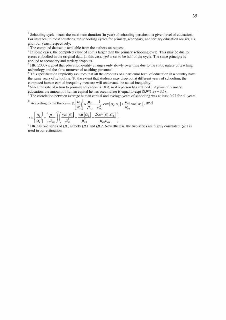
1 Schooling cycle means the maximum duration (in year) of schooling pertains to a given level of education. For instance, in most countries, the schooling cycles for primary, secondary, and tertiary education are six, six and four years, respectively. 2 The compiled dataset is available from the authors on request. 3 In some cases, the computed value of ypd is larger than the primary schooling cycle. This may be due to errors embodied in the original data. In this case, ypd is set to be half of the cycle. The same principle is applied to secondary and tertiary dropouts. 4 HK (2000) argued that education quality changes only slowly over time due to the static nature of teaching technology and the slow turnover of teaching personnel. 5 This specification implicitly assumes that all the dropouts of a particular level of education in a country have the same years of schooling. To the extent that students may drop out at different years of schooling, the computed human capital inequality measure will understate the actual inequality. 6 Since the rate of return to primary education is 18.9, so if a person has attained 1.9 years of primary education, the amount of human capital he has accumulate is equal to exp(18.9*1.9) = 3.58. 7 The correlation between average human capital and average years of schooling was at least 0.97 for all years. 8 According to the theorem, [ ] [ ]1 11
1 2 22 32 2 2 2
1cov , varα α
α α α
µ µα α α αα µ µ µ
Ε ≈ − +
, and
[ ] [ ] [ ]2
1 2 1 2112 2
2 2 1 2 1 2
var var 2cov ,var α
α α α α α
α α α αµαα µ µ µ µ µ
≈ + −
.
9 HK has two series of QL, namely QL1 and QL2. Nevertheless, the two series are highly correlated. QL1 is used in our estimation.