Embed Size (px)
Citation preview

Hugo Miguel Andrade Lopes Figueiredo da
Silva
Determination of the material/geometry of
the section most adequate for a static loaded
beam subjected to a combination of
bending and torsion
Guimarães, 2011

2

iii
ABSTRACT
The Finite Element Method (FEM) is widely used to solve structural analysis problems.
In this work, a novel Finite Element Model Updating methodology for static analysis is
presented. The aim of the work is to improve the quality of the results using the Finite
Element Updating techniques, by optimizing geometric parameters of the models and
material properties in order to minimize deflection. Deflection can be minimized by
increasing the Inertia moment of the section and/or Young modulus of the material. The
Young modulus can be optimized by selecting an adequate material. In this work,
material selection charts were used to determine the most reliable material. The selected
material was then tested by tensile and extensometry tests to obtain Young modulus,
Yield stress, and Poisson coefficient. The Inertia moment can be maximized by
improving the geometry of the section, such as adding ribs or webs. A substantial
improvement of the deflection can be achieved, but, in order to obtain the best results,
optimization must be used. A MATLAB program was used to optimize the ANSYS
models using a programming code. In order to know if the results are getting worse or
better in relation to the previous iterations, an objective function was defined. The
model is optimized when is not possible to further optimize the objective function.

iv
v
RESUMO
O método dos elementos finitos (FEM) é amplamente utilizado para resolver problemas
de análise estrutural estática. Neste trabalho é apresentada uma nova metodologia de
melhoria de modelos de elementos finitos para análise estática. O objectivo do trabalho
é melhorar a qualidade dos resultados utilizando as técnicas de melhoramento de
elementos finitos, através da optimização de parâmetros geométricos dos modelos e
propriedades do material, de modo a reduzir os deslocamentos. Os deslocamentos
podem ser minimizados através do aumento do momento de Inércia da secção e/ou
módulo de Young do material. O módulo de Young pode ser optimizado através da
escolha de um material adequado. Neste trabalho foram usadas cartas de selecção de
materiais para determinar o material mais adequado. Foram feitos ensaios de
extensometria e de tracção ao material seleccionado para obter as propriedades
relevantes do material: módulo de Young, tensão de Cedência e coeficiente de Poisson.
O momento de inércia pode ser maximizado melhorando a geometria da secção com
nervuras ou redes longitudinais. Uma melhoria substancial do deslocamento pode ser
obtida, mas, de modo a obter os melhores resultados, tem de se usar optimização. O
programa MATLAB foi utilizado para optimizar os modelos do ANSYS com um
código de programação. De modo a saber se os resultados estão a melhorar ou a piorar
em cada iteração, em relação às iterações anteriores, uma função objectivo foi definida.
O modelo está optimizado quando não é possível optimizar mais a função objectivo.

vi

vii
KEYWORDS
FINITE ELEMENT METHOD
FINITE ELEMENT MODEL UPDATING
OPTIMIZATION
STRUCTURAL STATIC ANALYSIS
MATERIALS SELECTION
MECHANICAL TESTS

viii

ix
ACKNOWLEDGMENTS
This work was a real pleasure, because it is strongly multi-subject, it gave to me
scientific knowledge in those subjects and it has practical applications.
I want to acknowledge:
-My scientific supervisor Professor José Filipe Meireles, for all the dedication, help, and
time spent in the orientation of my work.
-My father David, my mother Cidália, my sister Mara, my godmother Sónia, and my
friend Daniel Veiga, for the incredible support, encouragement, and belief in the
conclusion of this work.
-Mr. Araújo, material tests laboratory technician, for all the dedication in the
mechanical tests performed during this thesis.

x
xi
INDEX
ABSTRACT ........................................................................................................ iii
RESUMO............................................................................................................ v
KEYWORDS ..................................................................................................... vii
ACKNOWLEDGMENTS ..................................................................................... ix
CHAPTER 1-INTRODUCTION ........................................................................... 1
1.1 Motivation ..................................................................................................... 3
1.2 Aim of this work ............................................................................................ 4
1.3 State of the art .............................................................................................. 5
1.3.1 Rigidity and the Finite Element Method ................................................. 5
1.3.2 About Optimization methods .................................................................. 8
1.4 Context and purpose of the work and structure of the thesis........................ 9
CHAPTER 2-RELATED THEORY .................................................................... 11
2.1 Introduction to Finite Element Method ........................................................ 13
2.2 About ANSYS ............................................................................................. 15
2.3 Bending and Torsion loading ...................................................................... 15
2.3.1 Mechanical deflection .......................................................................... 16
2.3.1.1Differential elastic curve ................................................................. 16
2.3.1.2 Torsion deflection .......................................................................... 17
2.3.1.3 Total deflection .............................................................................. 21
2.4 Stresses in torsion and bending loading ..................................................... 21
2.5 Rigidity indices of materials ........................................................................ 22
2.6 Relation between structural rigidity and material properties ....................... 24
2.7 Mechanical tests ......................................................................................... 26
2.7.1 About tensile test ................................................................................. 26
2.7.2 Elastic and Plastic domains ................................................................. 27
2.7.3 Relevant properties obtained from a tensile test .................................. 28
2.7.3.1 Modulus of Elasticity ...................................................................... 28
2.7.3.2 Yield stress .................................................................................... 28
2.7.3.3 Rupture stress ............................................................................... 28
2.7.3.4 Elongation ..................................................................................... 28
2.7.3.5 Ultimate Tensile Strength .............................................................. 29
2.7.4 Determination of the Young modulus in tensile test ............................. 30
2.8 About MATLAB ........................................................................................... 31
2.9 Mathematical formulation of optimization methods ..................................... 32

xii
xiii
CHAPTER 3-EXPERIMENTAL PROCEDURE ................................................. 35
3.1 Materials selection ...................................................................................... 37
3.1.1 Initial selection ..................................................................................... 37
3.1.2 Intermediate material selection ............................................................ 39
3.1.3 Final material selection ........................................................................ 40
3.1.4 About commercial dual phase steels (High strength steels) ................ 41
3.1.4.1 Main characteristics ....................................................................... 41
3.1.4.2 About DOCOL dual phase steels .................................................. 42
3.2 Section Optimization .................................................................................. 44
3.2.1 Section Optimization: Main purposes................................................... 44
3.2.2 Section optimization: Longitudinal Webs ............................................. 45
3.2.3 Section optimization: Ribbing ............................................................... 47
3.3 FEM and Optimization ................................................................................ 50
3.3.1 Introduction .............................................................................................. 50
3.3.2 Finite Element Method experimental procedure .................................. 50
3.3.3 The FEM models ................................................................................. 52
3.3.4 Optimization Model .............................................................................. 54
3.3.5 The MATLAB program ......................................................................... 55
3.3.6 ANSYS Input file structure ................................................................... 59
4.1 Numeric approximation- Comparison between numeric and analytic methods ........................................................................................................... 63
4.1.1 About the model ................................................................................... 63
4.1.2 Beam Deflection by the Analytic method ............................................. 63
4.1.2.1 Bending ......................................................................................... 63
4.1.2.2 Torsion .......................................................................................... 64
4.1.2.3 Total deflection .............................................................................. 66
4.1.3 Beam Deflection by the numeric method ............................................. 66
4.1.4 Comparison of numeric and analytic methods ..................................... 67
4.2 Mechanical Tests ....................................................................................... 69
4.2.1 Denomination of the tested specimens ................................................ 70
4.2.1.1 Tensile test .................................................................................... 70
4.2.1.2 Extensometry test .......................................................................... 70
4.2.2 Tensile test experimental results ......................................................... 70
4.2.2.1 Stress-Strain and Stress-Extension charts .................................... 70
4.2.2.2 Determination of Young modulus in tensile test ............................ 70
4.2.2.3 Determination of Yield stress in tensile test ................................... 71
4.2.2.4 Determination of the Poisson coefficient, normal stress, and Young modulus in extensometry test .................................................................... 72

xiv

xv
4.3 Variable analysis ........................................................................................ 72
4.3.1 Variable analysis of model 1- ribbed plate ........................................... 74
4.3.2 Variable analysis of model 2- tubular beam ......................................... 74
4.4 Optimization results .................................................................................... 75
4.4.1 Model 1-Ribbed plate ........................................................................... 75
4.4.1.1 Initial variable values and limits ..................................................... 75
4.4.1.2 Geometric parameters optimization results ................................... 76
4.4.1.3 Material properties optimization results ......................................... 76
4.4.1.4 Optimization results using all variables ......................................... 77
4.4.2 Model 2- Tubular beam ........................................................................ 77
4.4.2.1 Initial variable values and limits ..................................................... 77
4.4.2.2 Geometric parameters optimization results ................................... 78
4.4.2.3 Material properties optimization results ......................................... 79
4.4.2.4 Optimization results using all variables ......................................... 79
4.5 Optimization settings .................................................................................. 80
4.6 FEM results ................................................................................................ 81
4.6.1 Model1: Ribbed plate ........................................................................... 81
4.6.1.1 Initial model results ........................................................................ 81
4.6.1.2 Geometric parameters ANSYS results .......................................... 81
4.6.1.3 Material properties ANSYS results ................................................ 82
4.6.1.4 ANSYS results using all variables ................................................. 83
4.6.2 Model2: Tubular beam ......................................................................... 83
4.6.2.1 Initial model results ........................................................................ 83
4.6.2.2 Geometric parameters ANSYS results .......................................... 84
4.6.2.3 Material properties ANSYS results ................................................ 85
4.6.2.4 ANSYS results using all variables ................................................. 86
CHAPTER 5-RESULTS DISCUSSION AND CONCLUSIONS......................... 87
5.1 Results discussion ...................................................................................... 89
5.1.1 Variable analysis .................................................................................. 89
5.1.1.1Material properties .......................................................................... 89
5.1.1.2 Geometric parameters ................................................................... 89
5.1.1.2.1 Model 1: ribbed plate ......................................................................... 89
5.1.1.2.2 Model 2: tubular beam ....................................................................... 90
5.1.2 Mechanical tests .................................................................................. 90
5.1.2.1 Extensometry test .......................................................................... 90
5.1.2.2 Tensile test .................................................................................... 90
5.1.3 Optimization results ............................................................................. 91

xvi
xvii
5.1.4 FEM results .......................................................................................... 91
5.1.5 Materials selection ............................................................................... 91
5.2 Conclusions of the work ............................................................................. 92
5.3 Future work proposals ................................................................................ 92
REFERENCES ................................................................................................. 95
Bibliographic references ................................................................................... 97
ANNEXES ...................................................................................................... 101
ANNEX 1-MECHANICAL TESTS ................................................................... 103
A1.0-Conditions of the Mechanical tests ........................................................ 105
A1.1-Stress-strain and stress-extension charts .............................................. 105
Specimen 1 ............................................................................................. 105
Specimen 2 ............................................................................................. 106
A1.2-Determination of Young modulus in tensile test ..................................... 107
Specimen 1 ............................................................................................. 107
Specimen 2 ............................................................................................. 108
A1.3-Charts used to determine Yield stress ................................................... 108
Specimen 1 ............................................................................................. 108
Specimen 2 ............................................................................................. 109
A1.4-Determination of Poisson coefficient and Young modulus in extensometry test ................................................................................................................. 109
ANNEX 2-VARIABLE ANALYSIS DATA ........................................................ 111
A2.1 Variable analysis data ............................................................................ 113
A2.1.1 Model 1- Ribbed plate ..................................................................... 113
A2.1.1.1 LG1 Variable ............................................................................. 113
A2.1.1.2 LG2 Variable ............................................................................. 114
A2.1.1.3 LG3 Variable ............................................................................. 115
A2.1.1.4 EX Variable ............................................................................... 116
A2.1.1.5 PXY Variable............................................................................. 117
A2.1.1.6 DNS Variable ............................................................................ 118
A2.1.2 Model 2- Tubular beam ................................................................... 119
A2.1.2.1 LG4 Variable ............................................................................. 119
A2.1.2.2 LG5 Variable ............................................................................. 120
A2.1.2.3 LG6 Variable ............................................................................. 121
A2.1.2.4 EX Variable ............................................................................... 122
A2.1.2.5 PXY Variable............................................................................. 123
A2.1.2.6 DNS Variable ............................................................................ 124
A2.2 Variable Analysis Charts ........................................................................ 125

xviii
xix
A2.2.1 Model 1: Ribbed plate ...................................................................... 125
LG1 variable ............................................................................................ 125
LG2 variable ............................................................................................ 125
LG3 variable ............................................................................................ 126
EX variable .............................................................................................. 126
PXY variable ........................................................................................... 127
DNS variable ........................................................................................... 127
A2.2.2 Model 2: tubular beam ..................................................................... 128
LG4 variable ............................................................................................ 128
LG5 variable ............................................................................................ 128
LG6 variable ............................................................................................ 129
EX variable .............................................................................................. 129
PXY variable ........................................................................................... 130
DNS variable ........................................................................................... 130
ANNEX 3-FINITE ELEMENT MODEL FILES ................................................. 131
A3.1-Model 1: ribbed plate ............................................................................. 133
A3.2-Model 2: Tubular beam .......................................................................... 141
ANNEX 4-SCIENTIFIC PAPER ...................................................................... 155
Abstract ........................................................................................................... 157
1. Introduction .................................................................................................. 157
2. Bending and torsion combined load ................................................................. 158
3. The FEM models ........................................................................................... 159
4. Optimization Model ....................................................................................... 160
5. Materials selection ......................................................................................... 160
6 Results ......................................................................................................... 161
6.1 Tensile test results ....................................................................................... 161
6.2 Extensometry test results .............................................................................. 162
6.3 Optimization results ..................................................................................... 162
7. Results discussion and conclusions.................................................................. 162
References ....................................................................................................... 163

xx
xxi
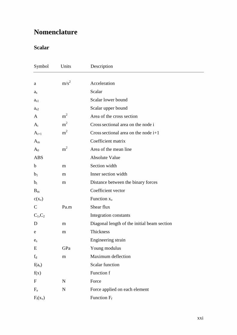
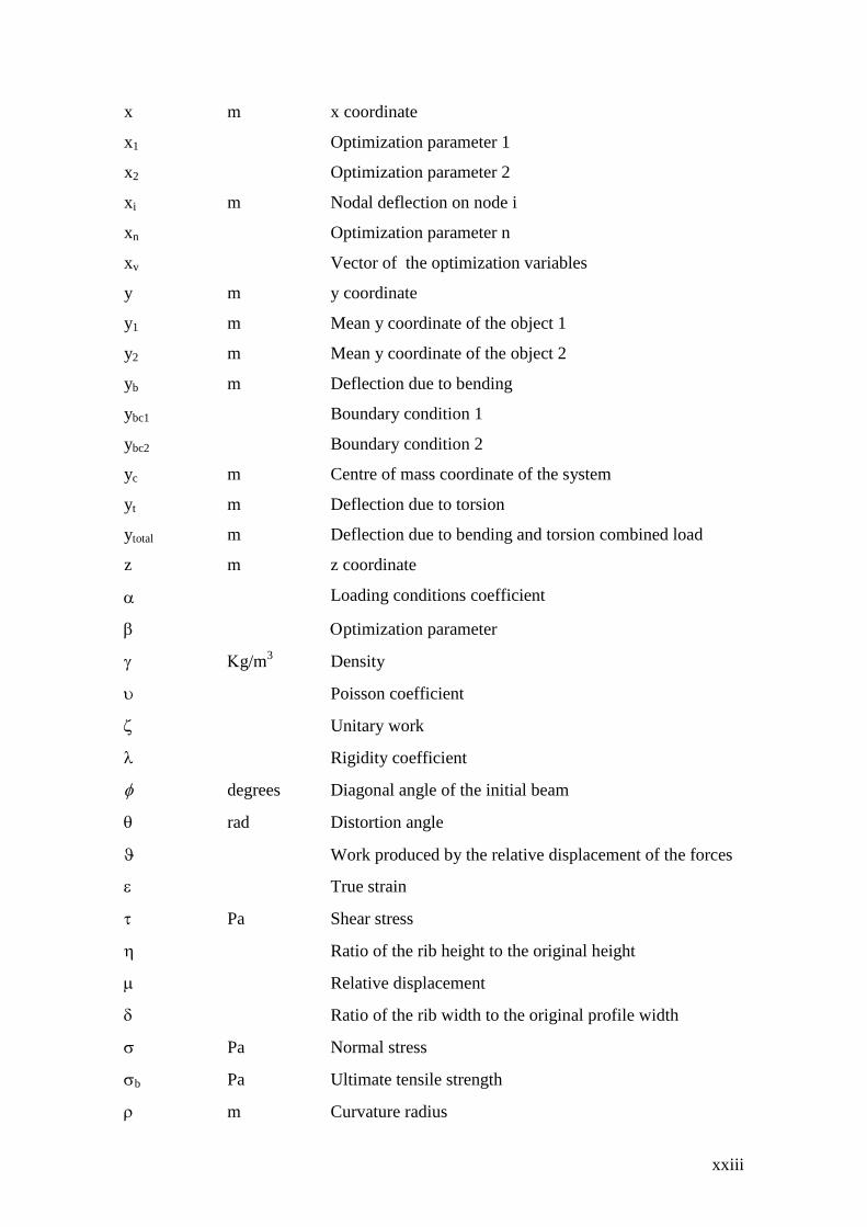
Nomenclature
Scalar
Symbol Units Description
a m/s2 Acceleration
as Scalar
as1 Scalar lower bound
as2 Scalar upper bound
A m2 Area of the cross section
Ai m2 Cross sectional area on the node i
Ai+1 m2 Cross sectional area on the node i+1
Am Coefficient matrix
A0 m2
Area of the mean line
ABS Absolute Value
b m Section width
b1 m Inner section width
bi m Distance between the binary forces
Bm Coefficient vector
c(xv) Function xv
C Pa.m Shear flux
C1,C2 Integration constants
D m Diagonal length of the initial beam section
e m Thickness
es Engineering strain
E GPa Young modulus
fd m Maximum deflection
f(as) Scalar function
f(x) Function f
F N Force
Fe N Force applied on each element
Ff(xv) Function Ff

xxii
F1 Binary load
g(x) Function g
G GPa Transversal Elasticity Modulus
h m Section height
h1 m Inner section height
h(x) Function h
H Quadratic programming optimization Matrix
I m4 Axial Inertia moment
Ip m4 Polar inertia moment
k Element stiffness
K(xv,w) Function K
l m Element length
lb Lower Bound
lt m Mean line perimeter
L m Length
Li m Instantaneous length of the specimen on tensile test
m kg Mass
m1 kg Mass of the object 1
m2 kg Mass of the object 2
ma Lower limit or upper limit constraints
me Equality constraints
mf Inequality constraints
Mf(x) N.m Bending moment
Mt N.m Torsion Moment
n Safety coefficient
q(x) m Objective function
r m Distance of the point to the action line of the force
s Slope of the recta
ub Upper bound
ui N Force on the elements at nodes i
ui+1 N Force on the elements at nodes i+1
V m3 Volume
w Weight of the optimization variables
W m3 Moment of resistance
xxiii
x m x coordinate
x1 Optimization parameter 1
x2 Optimization parameter 2
xi m Nodal deflection on node i
xn Optimization parameter n
xv Vector of the optimization variables
y m y coordinate
y1 m Mean y coordinate of the object 1
y2 m Mean y coordinate of the object 2
yb m Deflection due to bending
ybc1 Boundary condition 1
ybc2 Boundary condition 2
yc m Centre of mass coordinate of the system
yt m Deflection due to torsion
ytotal m Deflection due to bending and torsion combined load
z m z coordinate
Loading conditions coefficient
ptimization parameter
g/m3 Density
Poisson coefficient
Unitary work
Rigidity coefficient
degrees Diagonal angle of the initial beam
rad Distortion angle
Work produced by the relative displacement of the forces
True strain
Pa Shear stress
Ratio of the rib height to the original height
Relative displacement
Ratio of the rib width to the original profile width
Pa Normal stress
b Pa Ultimate tensile strength
m Curvature radius

xxiv
Subscriptions
Symbol Description
0 Initial
1 First
avg Relative to average value
0.2 Relative to Yield
eq Relative to equivalent
flex Relative to flexure (bending)
gen Relative to generalized rigidity index
l Relative to the lower limit
long Relative to longitudinal direction
trans Relative to transversal direction
tens Relative to tensile
total Relative to torsion and bending combined load
tors Relative to torsion
T Relative to transverse matrix
u Relative to the upper limit
xx Relative to the x axis
y Relative to y direction
Operators
Symbol Description
ds Distance between two points
dx 1st order differential of x coordinate
dy 1st
order differential of y coordinate
d2x 2
th order differential of x coordinate
d2y 2
th order differential of y coordinate
Variation
xxv
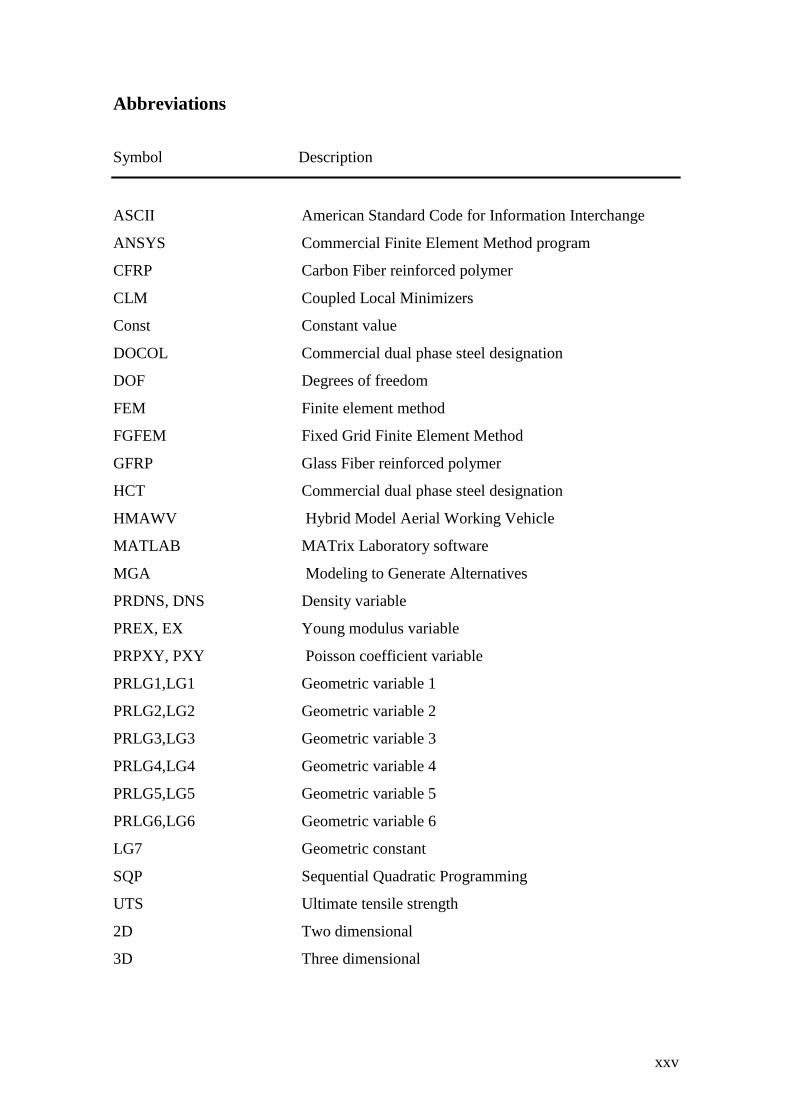
Abbreviations
Symbol Description
ASCII American Standard Code for Information Interchange
ANSYS Commercial Finite Element Method program
CFRP Carbon Fiber reinforced polymer
CLM Coupled Local Minimizers
Const Constant value
DOCOL Commercial dual phase steel designation
DOF Degrees of freedom
FEM Finite element method
FGFEM Fixed Grid Finite Element Method
GFRP Glass Fiber reinforced polymer
HCT Commercial dual phase steel designation
HMAWV Hybrid Model Aerial Working Vehicle
MATLAB MATrix Laboratory software
MGA Modeling to Generate Alternatives
PRDNS, DNS Density variable
PREX, EX Young modulus variable
PRPXY, PXY Poisson coefficient variable
PRLG1,LG1 Geometric variable 1
PRLG2,LG2 Geometric variable 2
PRLG3,LG3 Geometric variable 3
PRLG4,LG4 Geometric variable 4
PRLG5,LG5 Geometric variable 5
PRLG6,LG6 Geometric variable 6
LG7 Geometric constant
SQP Sequential Quadratic Programming
UTS Ultimate tensile strength
2D Two dimensional
3D Three dimensional


1
CHAPTER 1-INTRODUCTION

2
CHAPTER 1-INTRODUCTION
3
1.1 Motivation
The projects of industrial equipments have suffered severe changes, mainly because of
the increasing accelerations caused by electrical motors. Those motors are able to cause
movements with very high accelerations, sometimes going up to twelve times the
acceleration of gravity. The improvement of the movement capability makes necessary
an improvement on the resistance and rigidity of structures. The rigidity is one of the
basic factors that determine the working capability of equipments, and it usually has a
superior effect than resistance on the structure dimensioning. The deflection increase
due to high accelerations can cause problems on the equipment regular behaviour before
the lack of resistance is problematic. The lack of rigidity in structures causes an increase
of friction and wear in the mobile parts, but the main problem are the exaggerated
vibrations, which sometimes disturb the adequate operation. To improve rigidity it is
necessary to increase the Young modulus of the material and/or the Inertia moment of
the material section. The rigidity also depends of the geometrical characteristics, the
length of the object and the type of load. In the other hand, it is possible that some
composites, such as the glass fiber reinforcement polymer, even having a lower Young
modulus than most metals, could have a good mechanical behaviour, as well. Due to the
low density of those materials, one can strengthen the structure using more material, and
therefore, improve the inertia moment, having a low weight object as a result. The only
problem is the high cost of those materials, which are usually more expensive than any
commercial steel. The present work focuses the optimization of relevant parameters in
structural static analysis by the Finite Element Method. The tools used are the ANSYS
program, used for Finite Element modelling and the MATLAB program, used to run
and optimize ANSYS models, running a programming code written specifically for this
purpose.
CHAPTER 1-INTRODUCTION
4
1.2 Aim of this work
The main aim of this work is the development and analysis of a Finite Element Model
Updating application for structural static analysis to optimize the mechanical behavior
of the models when subjected to static combined loads. To achieve the aim, one must
optimize geometric parameters and material properties, with the goal of maximizing the
rigidity and minimizing the object mass. Rigidity is very important in what relates to
engineering parts, because it determines the work capability of engineering industrial
equipments. As told before, the importance of rigidity can be higher than resistance in
what relates to equipment reliability. To achieve this aim, one has to focus on two main
factors: The Young modulus and the Inertia moment. The Young modulus is only
dependent of the chosen material, and the Inertia moment is highly dependent on the
section of the object. In the other hand, a low mass is good because two factors: the
material cost and the admissible acceleration. According to Newton 2th
law (eq.1):
Fa=
m
(Eq. 1)
where:
a is the acceleration
F is the applied force
m is the mass
A lower mass can increase the admissible acceleration that is possible for a system, if
the Force F is kept constant. This is important because of the increasing accelerations of
new industrial equipments. In the other hand, a good mass position leads to a higher
inertia moment. Rigidity is of special importance in machines performing accurate
operations, such as metal cutting tools (example: Laser cutting), where the dimensional
precision of the final product must be as higher as possible. Rigidity is also very
important in some manufacturing machines, mainly those used commonly to
manufacture transport vehicles, aircraft and rockets. Special attention is given to rigidity
problems presenting high tensile strength or super-high tensile strength materials, where
those materials may drastically increase deflections. In fact, there is the tendency of
reducing the high-strength object thickness because the Yield stress is higher in high-
strength steels than in regular steel. However, their Young modulus is similar, which
CHAPTER 1-INTRODUCTION
5
means that if the material enters the plastic domain, the deflections should be similar if
the objects have the same dimensions. Therefore, if the thickness of a high-strength
steel object is decreased, there might be a drastic increase of deflection in comparison to
a similar object, made of regular steel but with a higher thickness [1]. The applications
of this work are the transversal beams of some industrial equipments, such as laser
cutting machines and plotters.
1.3 State of the art
1.3.1 Rigidity and the Finite Element Method
Rigidity can be defined as the capability of a mechanical system to deflect as less as
possible when subjected to external loads. If the rigidity of a system is higher in
comparison to other considering the same applied loads and the same material, the
deflections are lower. There are equations to evaluate the rigidity of structural parts by
means of a stiffness coefficient. The stiffness coefficient is the ratio between the load F
applied to a system and the maximum deformation f that results from the application of
the load. In the case of tension-compression of a beam with constant cross-section in
the elastic domain, the stiffness coefficient complies with Hooke´s law:
tensF EA
λ = =f L
(Eq. 2)
where:
tens is the rigidity coefficient in tension-compression
E is the Elasticity Modulus of the material
A is the area of cross section of the beam
L is the beam length measured along the action of the force
F is the applied load
f is the maximum deflection
When a beam with constant cross-section is subjected to torsion, the stiffness coefficient
is the ratio between the applied torque moment Mt and the twist angle (eq.3):
t ptors
M GIλ = =
θ L
(Eq. 3)

CHAPTER 1-INTRODUCTION
6
where:
tors is the rigidity coefficient in torsion
G is the Shear Modulus of the material
Ip is the polar moment of inertia of beam section
L is the beam length measured along the action of the force
Mt is the torsion moment
is the distortion angle
In the case of bending of a beam with constant cross-section, the stiffness coefficient
can be expressed by the eq. 4:
flex3
F αEIλ = =
f L
(Eq. 4)
where:
flex is the rigidity coefficient in bending
I is the axial inertia moment of the beam´s section
is a coefficient depending upon loading conditions
f is the maximum deflection
As described, the rigidity of the constructions is governed by the factors:
-E in tension-compression and bending and G in torsion
-The moment of inertia I or Ip respectively in bending or torsion loading
-Linear dimensions of the deformed body L
-Type of loading and type of supports
The elasticity is a very stable characteristic of the metals and depends uniquely of the
density of the atomic crystalline lattice (the mean inter-atomic distance). However, with
the development of composite materials, it has become possible to have multiple
materials in one object only with the aim of obtaining an adjustable mean Young
modulus. In these circumstances, this strategy can be considered, along with Inertia
moment improvement, the best practical way of improving rigidity of a system.
Particularly in thin walled structures, like plates and shells, the stability of the systems
is very important. One strategy that can be used against the lack of stability is the
reinforcement of easily deformable sections in the system by introducing stiffness limits
CHAPTER 1-INTRODUCTION
7
between the deforming section and the rigid units, and providing higher rigidity on
connecting points. Together with the increase in external sizes and decrease of wall
sections thickness it is necessary to increase rigidity in the transversal directions of
acting bending forces and torsion moments in order to avoid losses of construction
stability. Ribbing has wide application in improving rigidity, particularly in thin walled
components. Strength may significantly increase when one increase the rib thickness,
particularly at the critical regions. The influence of relative rib pitch and width of ribs
upon the rigidity and strength of a part is not easily expressed in a generalized form.
Because of this fact, an optimization process that can help the designer in the most
adequate selection between the existing valid solutions is very interesting and useful.
The use of numeric methods of calculus, such as the Finite Element Method (FEM),
controlled by optimization processes, can be a precious help in these cases [1]. There
are scientific works about the application of the Finite Element Method in structural
static and dynamic analysis. Y. Liu and L. Gannon wrote a paper entitled “Finite
element study of steel beams reinforced while under load”, consisting of reinforcing a
w-Shape steel beam with welded plates while under load. The Finite Element Method
was used for its modeling with the finality of investigate the effect of some parameters
related to the process [2]. Other authors, as G. Falsone, G. Ferro, demonstrated that “An
exact solution for the static and dynamic analysis of FE discretized uncertain structures”
can be obtained. The work is about the probabilistic analysis of FE discretized uncertain
linear structures in the static and dynamic structural analysis. The authors concluded
that the corresponding relationships between the response and the reduced number of
variables may be trivially deduced from the exact ones [3]. The Fixed Grid Finite
Element Method (FGFEM) method has been recently used by F. Daneshmand and M.
Kazemzadeh-Parsi to study the “Static and dynamic analysis of 2D and 3D elastic solids
using the modified FGFEM”. In this work a modification of the FGFEM is presented
and used for the static and dynamic analysis of 2D and 3D elastic solids. The accuracy
and convergence of the proposed method was analyzed via some numeric examples and
the results were compared with analytic and numeric solutions. The authors conclude
that the results show good agreement with the analytic and numeric solutions [4]. The
mechanical behavior of shells of revolution was studied in the work “Nonlinear static
and dynamic analysis of shells of revolution”, by C. Polat , Y. Calayir. In this work,
geometrically nonlinear static and dynamic response of shells of revolution is
investigated. During this work, a MATLAB code was developed to study geometrically

CHAPTER 1-INTRODUCTION
8
linear and nonlinear static and dynamic responses of shells of revolution. The authors
conclude that the nonlinearity affect the solutions significantly [5].
1.3.2 About Optimization methods
B. Zárate and J. Caicedo studied multiple alternatives to the Finite Element Model
Updating technique in the work “Finite element model updating: Multiple alternatives”.
The authors studied a Finite Element Model Updating methodology of complex
structural systems. Traditional Finite Element Model Updating techniques optimize an
objective function to calculate one single optimal model that behaves similarly to the
real structure and represents the physical characteristics of the structure. The author
have discovered that a local minimum, rather than the global minimum could be a better
representation of the physical properties of the structure, mainly due to numeric and
identification errors, as well as the limited number of sensors in structures. The
proposed method is based on MGA – Modeling to Generate Alternatives [6]. An
optimization method called “Coupled Local Minimizers” was used by P. Bakir, E.
Reynders, G. Roeck in the paper entitled “An improved Finite Element Model
Updating method by the global optimization technique ‘Coupled Local Minimizers’ “.In
this scientific work, a global optimization method called ‘Coupled Local Minimizers’
(CLM) is used for updating the Finite Element Model of a complex structure. The CLM
method is compared with other local optimization methods such as the Levenberg–
Marquardt algorithm, Sequential Quadratic Programming and Gauss–Newton methods
and the results show that the CLM algorithm gives better results in Finite Element
Model Updating problems compared to the above-mentioned local optimization
methods [7]. The paper “Discrete optimization problems of the steel bar structures”, by
S. Kalanta, J. Atkociunas, A. Venskus focus the optimal design problems of elastic and
elastic-plastic bar structures. These problems are formulated as nonlinear discrete
optimization. The main conclusions were: Elastic-plastic framed structure analysis
confirmed the statement that often an optimal structure project is determined not by the
strength, but the stiffness, stability and structural requirements, and, mathematical
models and solution algorithms for 2D optimization problems can be adopted for
solutions of 3D optimization problems [8]. X. Bin, C. Nan and C. Haunt have
implemented “An integrated method of multi-objective optimization for complex
mechanical structure”, where the authors present an integrated method of multi-
CHAPTER 1-INTRODUCTION
9
objective optimization for complex mechanical structures. It integrates prototype
modeling, FEM analysis and optimization. To explore its advantages over traditional
methods, optimization of a manipulator in hybrid mode aerial working vehicle
(HMAWV) is adopted. The results indicated that this integrated method is effective and
shows a potential in engineering applications. The authors concluded that this integrated
method of multi-objective optimization has solved a practical problem successfully, and
its efficiency has been improved greatly compared with enumerative methods [9]. Based
on the work of this thesis, a scientific paper was written and oral presented on VI
International Materials Symposium MATERIAIS 2011, held in University of Minho,
Guimarães (Annex 4) [10].
1.4 Context and purpose of the work and structure of
the thesis
The most important goal of this work is the minimization of nodal deflections due to
applied loads. Ribbing is an effective way of maximizing inertia moment. Therefore,
there is the need of optimizing ribbing-related variables, such as rib thickness, length
between consecutive ribs, and rib height, in the particular case of plate objects. When
those three parameters are optimized using a suitable objective function, one can
achieve good results. In the case of the tubular beam considered in this work, the
relevant variables are: distance from the center to the corner segment in each side;
length of the center segment, and height of the center segment. In the other hand,
material properties, such as Young modulus and Poisson coefficient also affect the
deflection results. Having this fact in consideration, all the variables were studied alone,
in order to know how its variation affects the value of the objective function. In chapter
1, the state of the art is presented, as well as the motivation and the aim of this work. In
chapter 2, the related theory is presented, including theory about mechanical tests,
equation demonstrations and optimization. In Chapter 3, the experimental procedure is
presented. This chapter is about the materials selection, section optimization, FEM
models and the MATLAB optimization program. The results are presented on chapter 4.
The chapter 4 is about mechanical tests results (tensile test and extensometry test),
variable analysis of the two finite element models (ribbed plate and tubular beam), FEM
results on ANSYS, and MATLAB optimization results (final values of the objective

CHAPTER 1-INTRODUCTION
10
function and variables). The optimization variables were six, in both models: three
variables are geometric, and three variables are material properties. The geometric
parameters are different in the two FEM models. However, the studied material
properties are the same for the two models. Chapter 5 is about the results discussion and
conclusions. It features mechanical tests, FEM, and optimization results discussion and
conclusions. The Annex 1 contains the tensile test and extensometry test charts,
featuring stress-strain charts, stress-extension charts, and charts used to determine two
mechanical properties of the material: Yield stress and Young modulus. In the Annex 1,
there are also the tables used to calculate Young modulus and Poisson coefficient in
extensometry test. In the Annex 2, one can see the variable analysis data, featuring
nodal deflection values and the charts obtained in the variable analysis. In the Annex 3
one can see the Finite Element Model input files, used to optimize the models on
MATLAB. In the Annex 4 there is the scientific paper published during this thesis.

11
CHAPTER 2-RELATED THEORY

12

CHAPTER 2-RELATED THEORY
13
2.1 Introduction to Finite Element Method
The Finite Element Method is a numeric procedure that can be used to obtain solutions
to a large number of engineering problems involving stress, deflection, heat transfer and
electromagnetic phenomena. The finite element method (FEM) consists in a computer
model that is analyzed under certain conditions. FEM is used either in new product
design, and existing product refinement. It is very useful to verify if a proposed design
will be able to perform to the client's specifications before manufacturing. A
modification in an existing product or structure is usually done with the purpose of
qualify the product or structure for a new service condition. In case of structural failure,
FEM may be used to help the design improvement in order to meet the new service
condition [11]. In the case of structural static analysis, which is the subject of this work,
the model is statically loaded. In this work, one is analyzing the elastic domain only,
due to the nature of the application. In the elastic domain, there is a linear relation
between stress and strain. The proportionality constant is the Young modulus E, as
shown next in eq. 5:
0
ΔLσ=Εε=E
L (Eq. 5)
where:
is theNormal stress
is the Strain
is the Young modulus
L is the length variation
L0 is the initial length of the object
In FEM, it is very important to assume a solution that approximates the behaviour of the
elements. Considering the deflection of a solid member with a uniform cross-section A,
a length L when subjected to a tensile Force F, one can say that the normal stress is
given by eq. 6:
Fσ=
A (Eq. 6)

CHAPTER 2-RELATED THEORY
14
where:
F is the applied force
A is the area of the cross-section
Using Eq. 5 and 6, one can obtain a new equation (Eq.7):
0
AEF= ΔL
L (Eq. 7)
The elastic behaviour of an element can be modelled by an equivalent linear spring
according to the eq. 8 [12]:
avg i+1 ie eq i+1 i i+1 i i+1 i
A E (A +A)EF =k (u -u )= (u -u )= (u -u )
l 2l (Eq. 8)
where:
Fe is the force on the elements
Ai and Ai+1 are the cross sectional areas of the member at nodes i and i+1
Aavg is the average area
l is the length of the element
ui and ui+1 are the forces on the elements at nodes i and i+1, respectively
The equivalent element stiffness is i+1 i
eq(A +A)E
k =2l
Despite the advantages of the FEM, it has limitations that can lead to errors in the
analysis results. In many practical engineering problems one cannot obtain exact
solutions. The difficulties to obtain exact solutions may be attributed to either the
complex nature of the governing differential equations or the difficulties that arise from
dealing with the boundary and initial conditions. The errors that contribute to the
models limitations can be divided into: User errors, due to mistakes in the data input
process, such as physical properties and dimensions, misuse of the selected elements,
misapplication of DOF constraints, low discretization of the geometry of the structure,
for example, due to an inappropriate rough mesh size or an inaccurate approximation of
geometries and inherent numeric methods errors used to solve the equilibrium
equations. These errors are due to the finite precision of the method, where conditions
are not controllable, or expected. For complex structures, even when using correct
meshes for each specific problem, errors can be substantial. These errors occur due to
difficulties in adapting the meshes to the geometry of the model [13].

CHAPTER 2-RELATED THEORY
15
2.2 About ANSYS
The implementation of the Finite Element Method usually follows three steps: Pre-
processing, solution and post-processing. Within these three basic steps, there are sub-
steps. In pre-processing, one defines the geometric model and builds the mesh with the
elements. In this work, the sequence of creating the geometric model was: keypoints,
then lines by keypoints and then areas by lines. The mesh makes possible the
discretization of the elements on the domain, by assigning to each element segment a
partial differential equation. All the differential equations are discretized after
integration in the area of the elements. The equations are then solved by algebraic
methods, such as gauss elimination method. In the solution menu it’s necessary to
define the loads and the DOF displacements (constraints). After solving the model, the
results can be viewed in the post-processing menu. For structural static analysis, as in
this work, the most important are the stresses and the deflections. This work has the aim
of obtaining the lowest possible deflections. Because of that, the results taken from the
program were the deflections. The stresses are also an indicator of the mechanical
behavior, since they are responsible for mechanical deflection. With FEM commercial
software, such as ANSYS, all these steps can be performed through graphical interfaces
or by command input.
2.3 Bending and Torsion loading
In practice is very common to find situations where the objects are loaded with a
combination of bending and torsion. Bending is usually due to central transverse load,
and torsion can be due to transverse load that is not centered. In some situations, these
two types of loading act at the same time, and so, one have a combination of bending
and torsion. In bending there are only normal stresses, and in torsion there are only
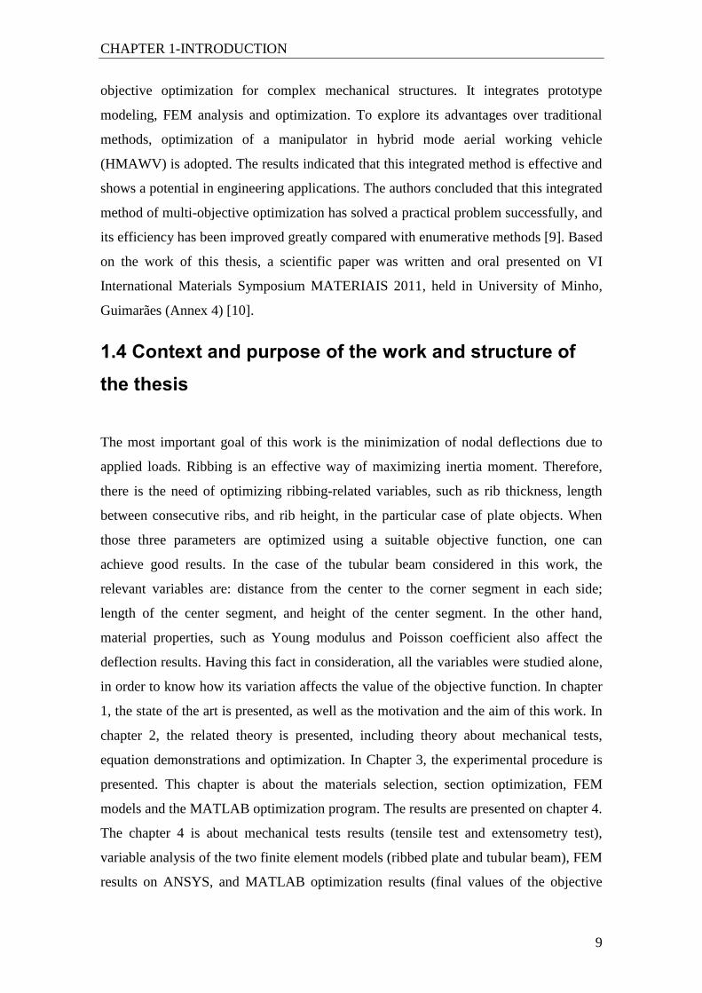
shear stresses. The next figure (fig. 1) shows the FEM model, its loading and DOF
constraints used in the preliminary analysis. The considered load was a centred bending
load F of 3528 N, which is 12 times the acceleration of gravity on a mass of 30 kg
(12*9,8*30=3528 N) and a binary load Mt=0,2*F1 that produces torsion, in which F1 is
equal to of 5120 N:
CHAPTER 2-RELATED THEORY
16
Fig. 1-Load applied to FEM models and DOF constrains
In torsion and bending combined loading, there are both shear stresses due to torsion
and normal stresses due to bending. The total deflection is the sum of the deflection due
to bending and the deflection due to torsion.
2.3.1 Mechanical deflection
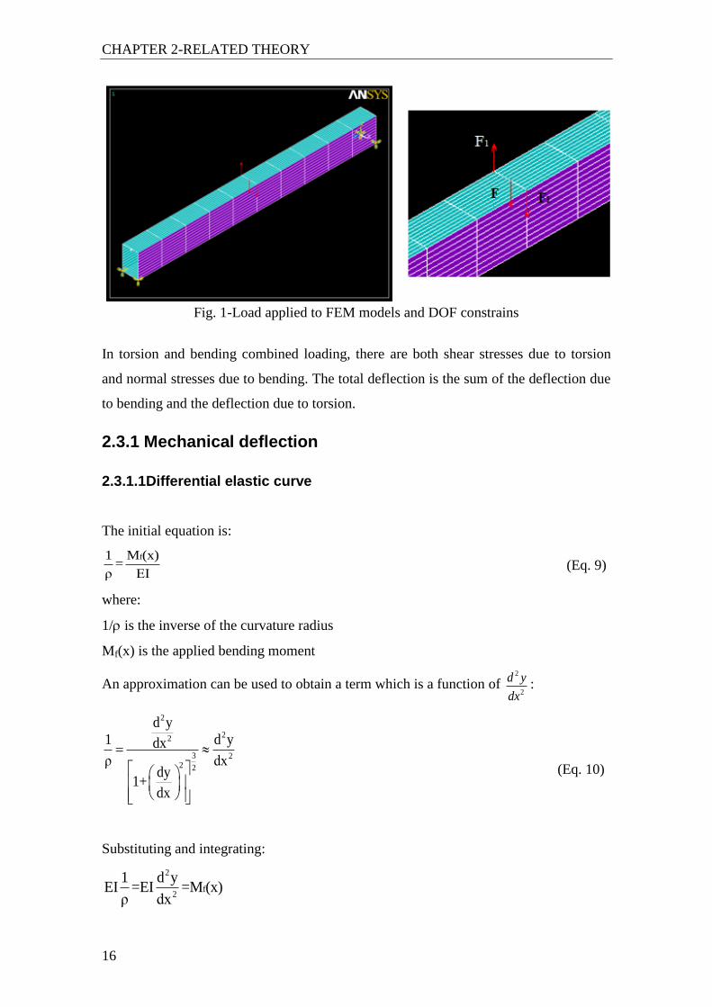
2.3.1.1Differential elastic curve
The initial equation is:
f1 M (x)=
ρ EI (Eq. 9)
where:
1/is the inverse of the curvature radius
Mf(x) is the applied bending moment
An approximation can be used to obtain a term which is a function of 2
2
d y
dx:
2
22
3 22 2
d y
1 d ydx
ρ dxdy
1+dx
(Eq. 10)
Substituting and integrating:
2
f2
1 d yEI =EI =M (x)
ρ dx
CHAPTER 2-RELATED THEORY
17
x
f 1
0
dyEIθ EI M (x)dx+C
dx
x x
f 1 2
0 0
EIy dx M (x)dx+C x+C
x x
f 1 2
0 0
EIy= dx M (x)dx+C x+C
Constants can be determined by applying boundary conditions. For a simply supported
beam, one has:
bc1 bc2y =0,y =0
The final equation used to obtain the deflection is:
3 2 3
b2 3
FL x xy = 3 -4
48EI L L
(Eq. 11)
where:
yb is the deflection due to bending
F is the applied load
L is the length of the object
x is the x coordinate
One can see that the deflection is dependent of both the geometry of the object (Inertia
moment I and length L) and the material (Young modulus E). The deflection is also
dependent on the load F and is a function of the x coordinate [14].
2.3.1.2 Torsion deflection
As a simplification, one can admit that the shear stress is constant along the thickness,
with a better accuracy the thinner the object is in relation to the dimensions of the
section. One can then demonstrate that the shear flux C=τt is constant, meaning that
the shear stress is constant if the thickness is constant.
If e,e1 are the thicknesses, and ,are the shear stresses in any two points m and n, it is
possible to know, by sectioning n and m, that those sections are subjected to shear
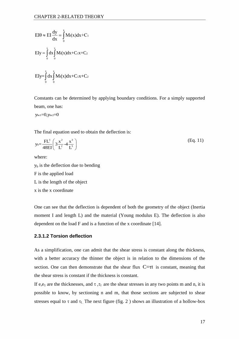
stresses equal to and The next figure (fig. 2 ) shows an illustration of a hollow-box
CHAPTER 2-RELATED THEORY
18
object, along with the representation of the shear stresses ,, the points m, n, the
thicknesses e, e1 and the distance between two points ds.
Fig. 2-Representation of a hollow-box object and relevant torsion parameters [15]
Considering two points located on the object wall, separated by a distance ds , the flux is
the same for the two points:
1 1C=τe=τ e (Eq. 12)
where:
C is the shear flux
is the shear stress
e is the object thickness
A face eds is subjected to a force τeds , and the moment of this force in relation to any
point of the section is τerds , where r is the distance of the considered point to the
action line of the force τeds . Considering that the sum of the moments in every point of
the wall should be equal to the torsion moment:
τerds=Mt
(Eq. 13)
Therefore, the flux τe can be expressed as a relation with the torsion moment tM :
tτe rds=M (Eq. 14)
The above equation (Eq. 14) represents the double of the area A0 of the inner side of the
mean line. Solving the integral, one can find the expression of the shear stress due to
torsion:
t
0
Mτ=
2A e (Eq. 15)

CHAPTER 2-RELATED THEORY
19
where:
is the shear stress
Mt is the torsion moment
A0 is the area of the mean line
e is the thickness
The unitary angle of torsion can be obtained by the laws of energy conservation, by
considering equal the work of deformation of a beam part with unitary length to the
inner work of the same part:
tM θξ=
2 (Eq. 16)
where:
is the unitary work
Mt is the torsion moment
is the twist angle due to torsion
The forces τeds applied to the horizontal faces of the volume element suffer the relative
displacement . The work produced by them is:
1= τeμds
2 . (Eq. 17 )
where:
is the work produced by the relative displacement of the applied forces
is the shear stress
e is the thickness
is the relative displacement
ds is the distance between the points n and m
Because the shear flux e on the vertical faces of the element moves perpendicularly to
it, the work produced by them is null. The inner work of the entire object is then:
21 1 τ
ξ1= τeμds= eds2 2 G
Considering the equation 16, one obtains:

CHAPTER 2-RELATED THEORY
20
2 2t t t2
2 2 20 0
M θ 1 1 M M ds= τ eds= eds=
2 2G 2G 4A e 8GA e
The distortion angle is then:
t
20
M dsθ=
4GA e (Eq. 18)
If the thickness is constant, then the equation 18, reduces to:
t t t
20 0
M l Clθ= =
4GA e 2GA e (Eq. 19)
where:
is the twist angle
C is the shear flux
lt is the mean line perimeter
G is the transversal elasticity modulus
A0 is the mean line area
e is the object thickness
Mt is the torsion moment
The deflection due to torsion can then be calculated [15]:
tD
y= θL2
(Eq. 20)
where:
yt is the deflection due to bending
D is the diagonal length of the object
L is the length
is the distortion angle
In the next figure (fig. 3), one can see an illustration of a hollow-box object subjected to
torsion:
Fig. 3-Hollow-box object subjected to torsion and relevant parameters
CHAPTER 2-RELATED THEORY
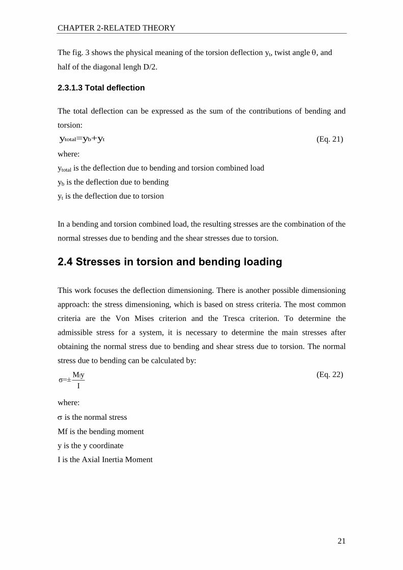
21
The fig. 3 shows the physical meaning of the torsion deflection yt, twist angle , and
half of the diagonal lengh D/2.
2.3.1.3 Total deflection
The total deflection can be expressed as the sum of the contributions of bending and
torsion:
total b ty =y +y (Eq. 21)
where:
ytotal is the deflection due to bending and torsion combined load
yb is the deflection due to bending
yt is the deflection due to torsion
In a bending and torsion combined load, the resulting stresses are the combination of the
normal stresses due to bending and the shear stresses due to torsion.
2.4 Stresses in torsion and bending loading
This work focuses the deflection dimensioning. There is another possible dimensioning
approach: the stress dimensioning, which is based on stress criteria. The most common
criteria are the Von Mises criterion and the Tresca criterion. To determine the
admissible stress for a system, it is necessary to determine the main stresses after
obtaining the normal stress due to bending and shear stress due to torsion. The normal
stress due to bending can be calculated by:
fM yσ=±
I
(Eq. 22)
where:
is the normal stress
Mf is the bending moment
y is the y coordinate
I is the Axial Inertia Moment

CHAPTER 2-RELATED THEORY
22
The shear stresses due to torsion in thin walled objects can be calculated by:
t
0
Mτ=
2tA (Eq. 15)
where:
is the shear stress due to torsion
Mt is the torsion moment (torque)
t is the beam thickness
A0 is the section mean line area
After obtaining the admissible stress by the chosen criteria, one must chose a material
with a Yield stress higher than the admissible stress as many times as the safety
coefficient n value.
2.5 Rigidity indices of materials
It is possible to obtain a generalized strength-rigidity index, by using the factors that
represent the weight advantage in terms of strength: 0.2σ
γ and rigidity advantage:
E
γ .
The generalized index is:
0.2gen
σ Eλ =
γ (Eq. 23)
where:
gen is the generalized rigidity index
0.2 is the yield stress
E is the Young modulus
is the density
This index represents the capability of a material to have the less deflection possible,
and less weight when subjected to high loads. The fig. 4 shows the value of the
generalized rigidity index for the most common engineering materials. The
correspondence of the material to the number is as follows:

CHAPTER 2-RELATED THEORY
23
Fig. 4-Generalized strength-rigidity indices [1]
According to the fig. 4, the materials can be separated in four groups:
1-Super high-strength steels ( gen 8*105)
2-Alloy steels, titanium alloys and sitalls( 3,5*105 gen 4*10
5)
3-Carbon steels, high strength cast irons and wrought aluminium alloys ( gen 1*105)
4-Structural bronzes, wrought magnesium alloys, cast aluminium alloys, cast
magnesium alloys, grey cast irons ( gen 0,5*105)).
In the table 1 one can see some properties of the most common structural materials,
along with their rigidity characteristics. The material with highest generalized rigidity
index is the high-strength steel, with a value of 8,4. The alloy steels are the second best,
but are much worse than the first, with a value of 3,8. Titanium alloys and Sitalls have a
value of 3,6, a value close to the alloy steels. The other materials have an index much
lower than titanium alloys. For some materials, the index is slightly higher than 1, but
for some materials it is substantially lower than one.

CHAPTER 2-RELATED THEORY
24
Materials
Density
(kgf/dm3
)
Modulus
of
elasticity
(kgf/mm2)
Rigidity
characteristi
c -3
b
E*10
σ
Generalized
factor
0.2 -5σ Ε*10
γ
Carbon Steels
7,85 21000
2,6 1,3
Alloy Steels 1,17 3,8
High-strenght Steels 0,6 8,4
Grey cast irons 7,2 8000 2,3 0,3
High-Strenght cast irons 7,4 15000 1,9 1,1
Aluminium
alloys
Cast 2,8 7200
2,9 0,45
Wrought 1,2 1,1
Magnesium
alloys
Cast 1,8 4500
2,1 0,32
Wrought 1,4 0,52
Structural Bronzes 8,8 11000 1,85 0,6
Titanium alloys 4,5 12000 0,8 3,6
Structural
plastics
Delta-
wood 1,4 4000 2 -
Glass-
fibers 1,6 5000 1,67 -
GFAM 1,9 6000 0,86 -
Sitalls 3 15000 1,87 3,6
Table 1-Strenght and rigidity characteristics of structural materials [1]
The material selection for a structural application is determined by the strength-rigidity
characteristics, but also by the relevant material properties for the considered
application. The mechanical design has a very high importance, because it´s possible to
build an object with high rigidity and strength, even when the material is not so stiff and
strong. The shape is therefore more relevant than the material for the mechanical
deflections reduction [1].
2.6 Relation between structural rigidity and material properties

CHAPTER 2-RELATED THEORY
25
The rigidity of the structures is determined by the deflection. The deflection is
dependent of the material properties and depends also of the geometric characteristics of
the object. The bending deflection due to transverse load can be expressed, as told
before, by:
3 2 3
b2 3
FL x xy = 3 -4
48EI L L
(Eq. 11)
where:
yb is the deflection (function of x coordinate)
I is the axial inertia moment of the section
E is the Young modulus of the material
L is the beams length
F is the applied load
x is the x coordinate
One can see that the material selection plays an important role in this work, since there
is a dependency of Young modulus on the deflection results. The results may vary
drastically if a different material is used, mainly in terms of the Young modulus. The
density is very important because the object mass is directly related to it:
mγ=
V (Eq. 24)
where:
is the density of the material
m is the material mass
V is the object volume
As Newton´s second law say that:
Fa=
m (Eq. 1)
where:
m is the mass of the material
a is the acceleration
F is the applied force
One can see that a lower mass can be important to obtain a good behavior of the
structure, since for a certain load, the lower the mass, the higher can be the acceleration

CHAPTER 2-RELATED THEORY
26
without structural failure, or/and undesirable vibrations. The density should be as low as
possible because for an object of the same dimensions, the mass is lower the lower is
the density. Two methodologies can be used in this work to achieve the goal of
deflection minimization:
- The Young modulus of the material must be the highest possible, because the
deflections are a function of it. This methodology is based on the importance of the
material properties. The high-strength steels, such as dual-phase steels, seem to be the
most suitable materials. This was the methodology used in this work.
- One can choose a material with not so high Young modulus, but with a
relatively low density and low/medium cost that allows the maximization of the Inertia
moment by means of object reinforcement with longitudinal webs or ribs. This
methodology is based on the improvement of the Inertia moment. Some suitable
materials for this methodology include composites, such as GFRP- Glass fiber
reinforced polymer.
2.7 Mechanical tests
2.7.1 About tensile test
A tensile test, also known as tension test, is the most relevant type of mechanical test
that can be performed on a material. It is used to determine the mechanical properties of
metals and metallic alloys. The main advantages of tensile tests are: simplicity, they are
relatively inexpensive, and fully standardized. As the test is performed, one will obtain
a stress-strain curve similar to what is shown next: (fig. 5)
Fig. 5-Typical stress-strain curve on a tensile test [16]
CHAPTER 2-RELATED THEORY
27
By performing this test, one can determine how the material reacts to the force being
applied, and consequently, one is able to obtain the material´s most important
properties, such as Young modulus, elongation, Yield stress, stress at rupture,
elongation until fracture (%), and area reduction until fracture (%). The results obtained
from the test can be used to build a normal stress-strain chart and a normal stress-
extension chart. The test specimens can be round, having 12,7 mm of diameter or can be
flat. When the original material has enough thickness, the specimens are usually round.
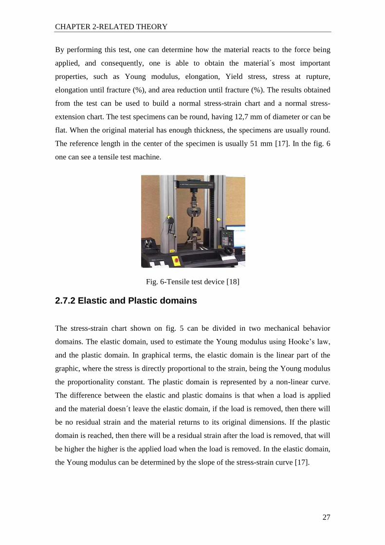
The reference length in the center of the specimen is usually 51 mm [17]. In the fig. 6
one can see a tensile test machine.
Fig. 6-Tensile test device [18]
2.7.2 Elastic and Plastic domains
The stress-strain chart shown on fig. 5 can be divided in two mechanical behavior
domains. The elastic domain, used to estimate the Young modulus using Hooke’s law,
and the plastic domain. In graphical terms, the elastic domain is the linear part of the
graphic, where the stress is directly proportional to the strain, being the Young modulus
the proportionality constant. The plastic domain is represented by a non-linear curve.
The difference between the elastic and plastic domains is that when a load is applied
and the material doesn´t leave the elastic domain, if the load is removed, then there will
be no residual strain and the material returns to its original dimensions. If the plastic
domain is reached, then there will be a residual strain after the load is removed, that will
be higher the higher is the applied load when the load is removed. In the elastic domain,
the Young modulus can be determined by the slope of the stress-strain curve [17].
CHAPTER 2-RELATED THEORY
28
2.7.3 Relevant properties obtained from a tensile test
2.7.3.1 Modulus of Elasticity
The modulus of elasticity is a measure of the stiffness of the material, but its
determination is only valid in the linear region of the stress-strain chart. Even in the
linear region of the chart, one cannot obtain the exact Young modulus, but an
approximation. The Young modulus is constant in every point of the linear region of the
stress-strain chart (elastic domain) [17].
2.7.3.2 Yield stress
The Yield stress of a material can be defined as the stress applied to the material at
which plastic deformation starts to be relevant when the material is loaded. Because
there is not a well defined point that is the end of the elastic domain region and the
beginning of the plastic domain, one usually chooses a Yield stress for a certain plastic
deformation. For structure projects, yield stress is usually calculated for a plastic
deformation of 0,002, which is 0,2%. Yield stress is usually calculated by making a line,
starting on the point 0,002 in the strain axis and stress equal to 0. The line is parallel to
the elastic domain curve. The point where the recta intersects the plastic domain of the
stress-strain curve is the Yield stress (stress axis) and Yield strain (strain axis) [17].
2.7.3.3 Rupture stress
Rupture stress is the current stress when the specimen suffers rupture. In projects with
ductile metallic alloys, the rupture stress is usually not an important value, because the
correspondent strain is very high. However, rupture stress can give an indication about
the presence of defects. When there are defects, such as pores or inclusions, the rupture
stress may be lower than the expected [17.]
2.7.3.4 Elongation
One is able to determine the amount of stretch or elongation the specimen suffers during
tensile test. This can be expressed as an absolute measurement in the change in length
called extension or as a relative measurement called "strain". There are two types of
strain, the "engineering strain" and "true strain". Engineering strain is probably the

CHAPTER 2-RELATED THEORY
29
easiest and the most common expression of strain used. It is the ratio of the change in
length to the original length:
0s
0 0
L-L ΔLe = =
L L (Eq. 25)
where:
es is the engineering strain
L is the final specimen length
L0 is the initial specimen length
The true strain is similar but based on the instantaneous length of the specimen as the
test progresses:
i
0
Lε=ln
L
(Eq. 26)
where:
is the true strain
Li is the instantaneous length
L0 the initial length.
The elongation is a measure of the material ductility. When the elongation is high, the
material ductility is usually high, and when the elongation is low, the material ductility
is usually low. The elongation can be obtained by joining the two parts of the specimen
that break during the tensile test and measuring the length. The initial length is usually
51 mm. The length should be delimited with a marker before the test, because one has
no way of measuring the elongation if this is not done [16].
2.7.3.5 Ultimate Tensile Strength
The ultimate tensile strength (UTS) is the maximum load the specimen sustains during
the test. The UTS may or may not be equal to the strength at break. This all depends on
what type of material one is testing: brittle, ductile, or a substance that even exhibits
both properties. The ductility depends on the conditions used, for example, sometimes a
material may be ductile when tested in a laboratory, but when placed in service and
exposed to extreme cold temperatures, it may suffer a transition to brittle behavior [17].

CHAPTER 2-RELATED THEORY
30
2.7.4 Determination of the Young modulus in tensile test
In tensile test, one obtained a results file. The results file has many columns, such as
time (in seconds), extension (mm), strain 2% (%), Load (N), Tensile Stress (MPa),
Tensile extension (mm), Tensile strain (%), displacement (Strain 2 in mm), True strain
%, position(mm),corrected position, toughness (gf/tex), and true stress (Pa).The results
are sorted by time, and each line corresponds to a time instant. The relevant results are
the extension, the strain 2%, and the load. By dividing the load by the transversal area
of the specimen one can find the nominal stress:
Fσ=
A (Eq. 6)
where:
F is the applied load
A is the transversal area of the specimen
is the normal stress
The Young modulus is given by equation 5:
σE=
ε (Eq. 5)
where:
E is the Young modulus
is the normal stress
is the strain
In order to determine Young modulus, one must do the linear fit of the stress-strain
chart for the elastic domain data. The equation used to perform the linear fit is:
cy=sx+b (Eq. 27)
where:
y is the y coordinate
x is the x coordinate
s is the slope of the recta
bc is the y coordinate on origin

CHAPTER 2-RELATED THEORY
31
Because the tested material is a dual-phase steel, the expected Young modulus for the
mechanical tests, either tensile and extensometry is 210 GPa, which is the regular value
for a steel.
2.8 About MATLAB
MATLAB is a technical computing environment for high performance numeric
computation and visualization. MATLAB features numeric analysis, matrix
computation, signal processing and graphics in an easy-to-use environment. MATLAB
features a family of solutions for specific applications called toolboxes. Toolboxes are
collections of MATLAB functions (M-files) that were pre-programmed in order to
extend MATLAB capabilities. MATLAB toolboxes can be related to many areas,
including optimization, signal processing, control design, dynamic systems simulation,
among others. In this work, the optimization toolbox was used in order to be possible to
use a required optimization function named fmincon [19]. There are many types of
optimization. According to the type of optimization (linear/nonlinear, constrained/non-
constrained), an objective function can be used for minimization or maximization. The
optimization toolbox consists of functions that can be applied to each particular case,
according to the optimization type. These routines require the definition of an objective
function. The following table (table 2) show the functions provided in the optimization
toolbox for different optimization problems.
Type Notation Function
Scalar Minimization s
s s1 s s2amin f(a ) such that a < a <a
fminbnd
Unconstrained Minimization v
vxmin f(x )
fminunc,
fminsearch
Linear Programming v
Tvx
m v m eq v eq b v b
min f x such that
A .x b , A .x =b , l x u
linprog
Quadratic Programming
v
T Tv v vx
m v m eq v eq b v b
1min x Hx +f x such that
2
A .x b , A .x = b , l x u
quadprog
Constrained Minimization v
v eq v
m v m eq v eq b v b
min f(x ) such that
c(x ) 0, c (x )= 0
A .x b , A .x = b , l x u
x
fmincon

CHAPTER 2-RELATED THEORY
32
Goal Attainment ,
v
v eq v
m v m eq v eq b v b
min such that
F(x ) = w. goal
c(x ) 0, c (x )= 0
A .x b , A .x = b , l x u
vx
fgoalattain
Minimax ( ) { }
v eq v
m v m eq v eq b v b
min max { } such that
c(x ) 0, c (x )= 0
A .x b , A .x = b , l x u
vf
f xx F F
fminimax
Semi-Infinite Minimization v
v
v eq v
m v m eq v eq b v b
min f(x ) such that
K(x ,w) 0 for all w
c(x ) 0, c (x )= 0
A .x b , A .x =b , l x u
x
fseminf
Table 2- MATLAB Minimization functions [20]
In this work, the function fmincon was used to optimize the objective function. The
function fmincon is used for “constrained minimization” optimization type [20].
2.9 Mathematical formulation of optimization methods
To achieve an optimal solution one must understand the mathematical formulation of
the optimization methods, since it is needed to establish correct mathematical
conditions. Optimization techniques are used to determine a set of parameters
Tx=[x1,x2..xn] that can be defined as optimum in certain conditions. Those parameters
are the optimization variables. An objective function q(x) is subject to a process of
minimization or maximization, which can be linear or non-linear, and constrained or
non-constrained. The constraints are functions that restrict the optimization variables,
and can be of three types: equality constraints, inequality constraints, and upper/lower
limit constraints as shown next:
ig (x) 0 e(i=l,...,m ) ; with me equality constraints
jh (x) 0 f(j=l,...,m ) ; with mf inequality constraints
l uk k ax ,x (k=l,...,m ) , with ma lower limit or upper limit constraints
An optimization problem is usually described by the minimization (or maximization) of
the objective function q(x):
min q(x)
subjected to the constraints conditions:
g(x)=0

CHAPTER 2-RELATED THEORY
33
h(x) 0
l ux x x
where:
x is the vector of the optimization parameters
q(x), g(x) and h(x) are functions.
To achieve an efficient solution, one must consider not only the number of constraints
and optimization variables, but also the characteristics of the objective and constraining
functions. In linear programming, all the optimization functions have linear behavior. In
quadratic programming, a quadratic function is minimized or maximized and linearly
constrained. For both optimization types, there are numeric procedures to obtain the
solution. For non-linear optimization, there is the need to run an iterative procedure,
achieved by the solution of a linear programming, quadratic programming, or even a
non-constrained optimization problem. The objective function q(x) has the purpose of
establishing a relation between the objective of the project and its variables. Such
variables can be material properties or geometric parameters. In this work, both material
properties and geometric parameters are the optimization variables. Usually, the
variables have linear behavior, but, if at least a single variable has non-linear behavior,
non-linear programming must be used [13].

34

35
CHAPTER 3-EXPERIMENTAL PROCEDURE

36

CHAPTER 3-EXPERIMENTAL PROCEDURE
37
3.1 Materials selection
3.1.1 Initial selection
The first step in the materials selection is the identification of the relevant properties of
the application. For this application the relevant properties are:
- Young modulus
- Toughness
- Inertia moment
- Cost of the material (cost of matter and manufacturing process)
- Density
The desired properties are:
- Young modulus (highest possible)
- Toughness (highest possible)
- Inertia moment (highest possible)
- Cost of the material (lowest possible)
- Density (lowest possible)
There are some properties that depend on the material, and some that are independent of
the material. This independency is shown next:
- Young modulus (dependent)
- Toughness (dependent)
- Inertia moment (independent)
- Cost of the material (dependent)
- Density (dependent)
The inertia moment is not dependent of the material. In fact, the inertia moment depends
of the geometrical characteristics of the objects, and doesn´t depend on which specific
material is chosen.

CHAPTER 3-EXPERIMENTAL PROCEDURE
38
For the materials selection one can only focus the material dependent properties. For the
first materials selection it is necessary to choose a material class, not a specific material.
This is true because one has more mobility to change to a material in the same class
with better properties for the application. The materials selection was done using
materials selection charts. In those charts one has two properties in 2 axes (2D) and
inside the chart there are the materials classes. This kind of diagrams make the materials
selection more organized, more simple and more effective than other methods, for
example, search in handbooks for reliable materials for a specific application. The
charts used for the first selection of the material were the Young modulus/Cost and
Young modulus/density. They are shown next (fig. 7) and (fig. 8):
Fig. 7-Materials selection chart Young modulus/density [21]
In this chart (fig. 7), one should select a class of the closest possible to the top left
corner (ideally) to obtain the highest possible Young modulus and lowest possible
density. There are no such materials, so one must look and find the best existing classes.
They are the ceramics, the composites and the metals. The ceramics are too brittle for
this application, the composites are too expensive, although GFRP- Glass Fiber
Reinforced Polymer is not very expensive in absolute terms, costing slightly more than
two Euros a kilogram [21], it is expensive comparing to most of the common metals.
The CFRP- Carbon Fiber reinforced Polymer is very expensive, with a cost of more
than 23 Euros a kilogram [21]. The metals have a high Toughness and high Young

CHAPTER 3-EXPERIMENTAL PROCEDURE
39
modulus. The only problem is they have a high density. But one can choose a specific
material inside the class that has a relatively low density to improve this.
Fig. 8-Materials selection chart Young modulus/Cost [21]
In this chart (fig. 8), one should select a material´s class that is the closest possible to
the up left corner as in the previous chart to obtain the highest possible Young modulus
and the lowest possible cost. As in the previous chart, there is no such material class.
The best material classes are: Metals and alloys, the Composites and the Ceramics. The
Composites have lower Young modulus than the Metals, and their cost is higher, so
they are not the best choice. The composites have a much lower density but with a
higher cost. The selection of the composites is only suitable for high performance
applications where the equipment cost is high, like boats. The ceramics, as told, are
brittle and they may fracture easily in an application such as this one. One can then
conclude that in the current state of art, the best material class is the Metals and Alloys,
which is the best class in both charts [21].
3.1.2 Intermediate material selection
If one details the Young modulus/density diagram (fig. 9), one sees that the best
materials for this application are: Steel, Cast Iron and Nickel, whose have a high Young
modulus and a relatively low density (they have the best relation between the two
properties).
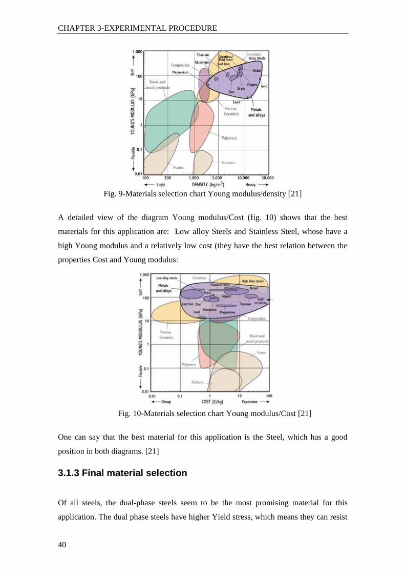
CHAPTER 3-EXPERIMENTAL PROCEDURE
40
Fig. 9-Materials selection chart Young modulus/density [21]
A detailed view of the diagram Young modulus/Cost (fig. 10) shows that the best
materials for this application are: Low alloy Steels and Stainless Steel, whose have a
high Young modulus and a relatively low cost (they have the best relation between the
properties Cost and Young modulus:
Fig. 10-Materials selection chart Young modulus/Cost [21]
One can say that the best material for this application is the Steel, which has a good
position in both diagrams. [21]
3.1.3 Final material selection
Of all steels, the dual-phase steels seem to be the most promising material for this
application. The dual phase steels have higher Yield stress, which means they can resist

CHAPTER 3-EXPERIMENTAL PROCEDURE
41
higher stresses without entering the plastic domain. In the plastic domain, unlike the
elastic domain, stress is not proportional to the strain and the strain is not totally
relieved after removal of the load. As in this application one desires that the object
works all the time in the elastic domain, this material seems to be highly suitable for this
application. The commercial dual phase steel DOCOL is the selected material. With the
dual phase steels it can be possible to obtain lower area sections having enough
mechanical resistance for the involved solicitations.
3.1.4 About commercial dual phase steels (High strength
steels)
3.1.4.1 Main characteristics
The main incentive for adopting dual phase steels for engineering structures
manufacture is the significant reduction in processing costs that are possible. The three
major direct cost savings are: no spheroidisation anneal, no quench and temper
treatment and no post Q&T descaling necessary. The Dual-phase steel has a soft ferrite
microstructure, with a matrix containing islands of martensite (increasing yield to
tensile strength) in the secondary phase (with proportional volume fraction increase in
analogue to tensile strength.) The fig. 11 shows the microstructure of some commercial
steels of this type, known as HCT:
Fig. 11-Microstructure of commercial dual phase steels [22]

CHAPTER 3-EXPERIMENTAL PROCEDURE
42
This type of steel features a low yield to tensile strength ratio, high tensile strength and
high work hardening rate. The high tensile strength is mainly achieved by the
composition, with manganese, chromium and silicone. The increase of the yield to
strength ratio in the martensitic phase is achieved by quenching the material before it
enters the zinc pot of the hot-dip galvanization unit. In the next figure (fig. 12) one can
see the Stress-Strain Curves for HCT commercial dual phase steels:
Fig. 12-Stress/Strain curves of some commercial dual phase steels [22]
The Stress-Strain curves are an excellent way to describe some of the most important
mechanical properties of materials. In the above figure (fig. 12), one can see the
mechanical behaviour of HCT450XD, HCT500XD and HCT600XD. It is notorious that
their Young modulus is similar, because the elastic domain slope is similar, but their
yield stress is quite different. The HCT600XD steel has the highest yield stress of all
three materials shown in the chart (fig. 12) [22].
3.1.4.2 About DOCOL dual phase steels
Below (table 3) one can see the chemical composition of the DOCOL dual phase steels.
Each steel designation number is related to tensile strength, eg. A DOCOL600 has a
tensile strength of near 600 [23].

CHAPTER 3-EXPERIMENTAL PROCEDURE
43
Table 3-Chemical composition of some dual phase commercial steels [23]
The mechanical properties of these steels are shown in the next table (Table 4):
Table 4-Mechanical properties of some dual phase commercial steels [23]
One can see that the Yield stress is presented in a range of values. Also, there is not a
determined value for Young modulus. Therefore, there is the need to perform
mechanical tests to determine a value for the Young modulus (extensometry test and
tensile test) and for the Yield stress (tensile test). Poisson coefficient was also
determined, due to its relevancy in the material deflection (extensometry test). In the
Annex 1, one can see the Young Modulus, Poisson coefficient and Yield stress obtained
in tensile test and extensometry test. The obtained values for the Young modulus are
smaller than the expected 210 GPa for all specimens. The Poisson coefficient is also
smaller than the expected 0,29 for all specimens, but the values are very close to the
expected value for most of the specimens.
CHAPTER 3-EXPERIMENTAL PROCEDURE
44
3.2 Section Optimization
3.2.1 Section Optimization: Main purposes
For the purpose of this work, rigidity is more important than resistance in what relates
to its structural applications. The bending deflection yb is a function of the bending
moment Mf(x), the axial inertia moment I and the Young modulus E. It is directly
proportional to Mf(x) and inversely proportional to I and E. However, in order to
decrease deflection, it´s important to choose a material with high Yield Stress, because
with a material having high Yield stress, it´s possible to reduce the object weight using
a lower thickness and then improve the Inertia moment of the section with ribs,
resulting in a lower deflection with a similar material cost. The bending deflection
equation results from double integration of the eq. 28, using the appropriate boundary
conditions, as shown in chapter 2:
2b f
2
d y M (x)=
dx IE (Eq. 28)
To increase rigidity one must increase the axial inertia moment I, as well as the Young
modulus E. The aim is to obtain a minimal deflection yb. There are ways of increasing
the Inertia moment. One is by the use of webs inside the object, the other is by the use
of ribs. Ribbing is usually less expensive than webs because of material costs (material
required to web a structure is usually more than to rib the same structure). The increase
of the axial Inertia moment of a modified object (usually ribbed or webbed) in
comparison with the initial object is defined by the ratio I/I0. As an example: a ratio of 2
means that the reinforced object has twice the inertia moment in comparison to the
initial object. Ribbing is usually more effective in terms of I/I0 than webbing. The
higher I/I0 one has in the ribbed structure, the higher the Inertia moment will be in
comparison to the inertia moment of the initial structure (non-ribbed). As a result of the
improvement of the Inertia moment, there is higher rigidity and consequently, lower
deflections. In fig. 13, one can see a ribbed plate FEM model:

CHAPTER 3-EXPERIMENTAL PROCEDURE
45
Fig. 13-Example of a ribbed plate
However, there are implications in the use of ribbing. The most critical implication is
the deflection increase due to wrong ribbing. Also important is the mechanical
resistance, due to high shear stresses in the ribs joints caused by transverse loads,
especially when the rib thickness is low [1].
3.2.2 Section optimization: Longitudinal Webs
About longitudinal webs, the theory says that the best improvement obtained by adding
longitudinal webs is achieved when there are two longitudinal webs, as in fig. 15. It was
found in the literature that the webs minimize the lower deflections and stresses while
almost not affecting the others, and ribs lower the high deflections and stresses while
almost not affecting the lowers. The next figure (fig. 14) shows the possible types of
longitudinal webs and the correspondent improvement of the axial inertia moment I.
Fig. 14-Effect of longitudinal webs on Inertia moment [1]
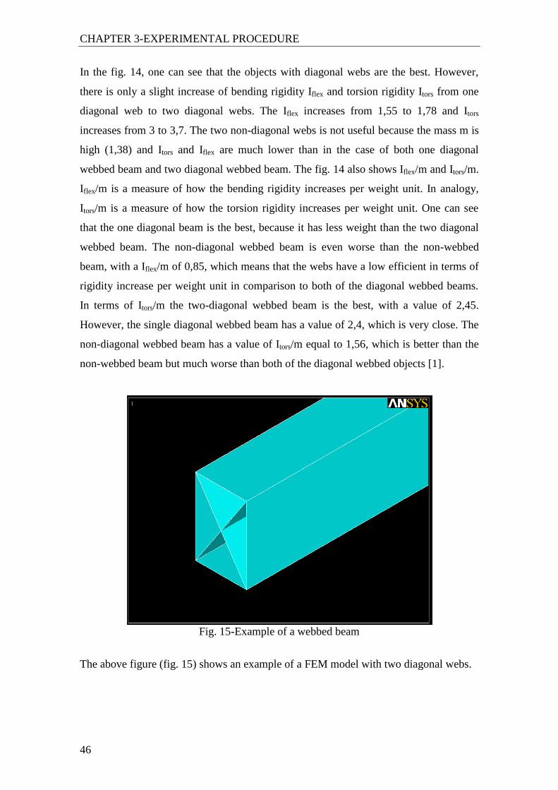
CHAPTER 3-EXPERIMENTAL PROCEDURE
46
In the fig. 14, one can see that the objects with diagonal webs are the best. However,
there is only a slight increase of bending rigidity Iflex and torsion rigidity Itors from one
diagonal web to two diagonal webs. The Iflex increases from 1,55 to 1,78 and Itors
increases from 3 to 3,7. The two non-diagonal webs is not useful because the mass m is
high (1,38) and Itors and Iflex are much lower than in the case of both one diagonal
webbed beam and two diagonal webbed beam. The fig. 14 also shows Iflex/m and Itors/m.
Iflex/m is a measure of how the bending rigidity increases per weight unit. In analogy,
Itors/m is a measure of how the torsion rigidity increases per weight unit. One can see
that the one diagonal beam is the best, because it has less weight than the two diagonal
webbed beam. The non-diagonal webbed beam is even worse than the non-webbed
beam, with a Iflex/m of 0,85, which means that the webs have a low efficient in terms of
rigidity increase per weight unit in comparison to both of the diagonal webbed beams.
In terms of Itors/m the two-diagonal webbed beam is the best, with a value of 2,45.
However, the single diagonal webbed beam has a value of 2,4, which is very close. The
non-diagonal webbed beam has a value of Itors/m equal to 1,56, which is better than the
non-webbed beam but much worse than both of the diagonal webbed objects [1].
Fig. 15-Example of a webbed beam
The above figure (fig. 15) shows an example of a FEM model with two diagonal webs.

CHAPTER 3-EXPERIMENTAL PROCEDURE
47
3.2.3 Section optimization: Ribbing
The next figure (fig. 16) shows how ribs affect the moment of resistance W and the
axial inertia moment I of beams. The moment of resistance W of a non-ribbed section is
considered to be unitary.
Fig. 16-Effect of Ribs on the inertia moment and W [1]
About ribbing, one can say that the best rib section has W=180 and I=300 as shown in
the fig. 16. The rib sections on the left side of the fig. 16 don´t have enough thickness
and/or height. Due to this fact, the resistance moment W is equal or less than 1 for all
cases, except for one case, that W wasn´t determined. However, for some rib sections,
there is a substantial increase of the inertia moment, with values of 4,5 for the last rib
sections, and 7,8 for the fifth rib section. In the right side of the fig. 16, one can see that
the second, third and forth solutions have a W=2 and a I of 21 for the second and 11 for
the third and forth. The second best rib section is the fifth on the right side, with a W of
5 and a I of 35. The influence of rib height and rib thickness on the Inertia moment and
moment of resistance can be expressed in a generalized form. For the inertia moment,
the expression is:
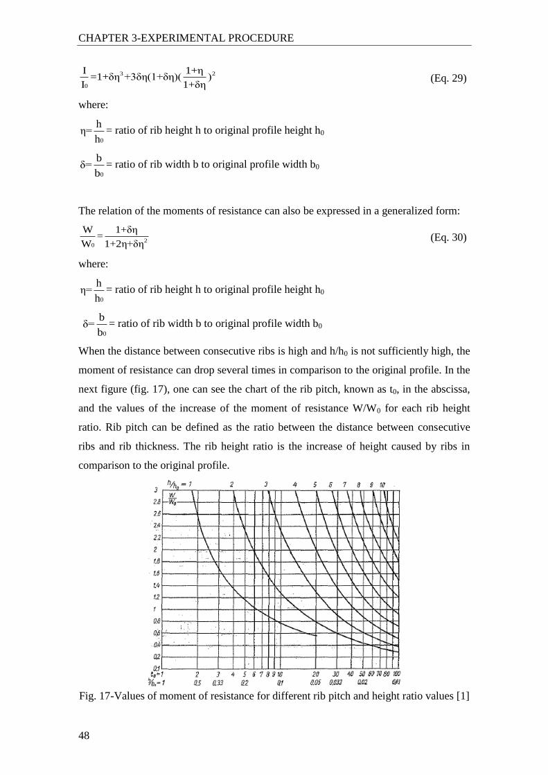
CHAPTER 3-EXPERIMENTAL PROCEDURE
48
3 2
0
I 1+η=1+δη +3δη(1+δη)( )
I 1+δη (Eq. 29)
where:
0
hη=
h= ratio of rib height h to original profile height h0
0
bδ=
b= ratio of rib width b to original profile width b0
The relation of the moments of resistance can also be expressed in a generalized form:
20
W 1+δη=
W 1+2η+δη (Eq. 30)
where:
0
hη=
h= ratio of rib height h to original profile height h0
0
bδ=
b= ratio of rib width b to original profile width b0
When the distance between consecutive ribs is high and h/h0 is not sufficiently high, the
moment of resistance can drop several times in comparison to the original profile. In the
next figure (fig. 17), one can see the chart of the rib pitch, known as t0, in the abscissa,
and the values of the increase of the moment of resistance W/W0 for each rib height
ratio. Rib pitch can be defined as the ratio between the distance between consecutive
ribs and rib thickness. The rib height ratio is the increase of height caused by ribs in
comparison to the original profile.
Fig. 17-Values of moment of resistance for different rib pitch and height ratio values [1]

CHAPTER 3-EXPERIMENTAL PROCEDURE
49
One can say that for some values of rib pitch and height ratio there is a decrease of the
moment of resistance W. This happens when W/W0 < 1. The object will be weaker if
the rib height decreases, and/or if there is a higher rib pitch. There are three ways of
increasing rigidity of a ribbed structure: one has to increase rib height, to decrease rib
pitch, or to increase rib thickness. Ribbing has shown to be a better way to improve the
rigidity of beams than longitudinal webs. It is better in what concerns to material cost
and in what concerns to deflections. However, one must consider the processing of the
ribs. As the material processing of the ribs requires more structural detail, it is more
expensive than webs (using the same processing method to be able to compare). This
cost can be relatively high, if the ribbing structure has many ribs [1]. In the next
illustration (fig. 18) one can see a ribbed structure.
Fig. 18-Example of a ribbed beam
This sub-chapter was the base for the selection of the variables of the ribbed plate
model. It was shown that rib thickness, rib height and rib pitch can substantially affect
the deflection of ribbed objects, by influencing the rigidity and the resistance. The
distance between consecutive inner ribs is represented on the ribbed plate model by the
LG1 variable, the rib height is represented by the LG2 variable and the thickness is
represented by the LG3 variable. Rib pitch concept was applied to the ribbed plate FEM
model as the distance between consecutive inner ribs, for a question of simplicity. There
is no need to define the ratio of distance between consecutive inner ribs divided by the
thickness, and one can apply the rib thickness only to one variable (LG3).

CHAPTER 3-EXPERIMENTAL PROCEDURE
50
3.3 FEM and Optimization
3.3.1 Introduction
Nowadays, the engineering structures usually have a high level of complexity. The
numeric methods, such as the FEM- Finite Element Method, are very useful to test if the
engineering object specifications are adequate for the working conditions of the
application. In the case of this work, the aim is to reduce the nodal deflections as much
as possible in the FEM models. The commercial FEM software used was ANSYS.
ANSYS can itself give deflection solutions. However, the aim is to reduce the
deflections as much as possible. To be possible to achieve the aim, one has to use
another program, called MATLAB (MATrix LABoratory) to optimize the models. A
programming code was developed in this work for the control of the optimization
processes. MATLAB is responsible for the control of the optimization processes, by
collecting deflection data from the text file l5.glw that is filled by ANSYS,
optimizing the variable values, and re-sending the model input file MODnume.txt
with the new variable values to ANSYS to be re-analyzed. This process can be done as
many times as needed to achieve an optimum solution, in an iterative process. The
ANSYS input file is a text file with all instructions related to the model construction.
The input files must be edited in order to have: the variables in the keypoints, the initial
variable values, and to write the deflection results in the nodal points to a file named
n5.lgw, used by MATLAB to calculate the objective function.
3.3.2 Finite Element Method experimental procedure
The ANSYS program is divided mainly in 3 sections: Pre-processor, Solution and Post-
processing:
-Modelling, definitions and meshing in Pre-processor
-Loads, DOF constraints and solution (solving) in Solution section.
-Plot results and query results (Total Strain) in Post-processing.
The steps to create and solve the FEM models were:
Preprocessor
Modelling
CHAPTER 3-EXPERIMENTAL PROCEDURE
51
Creation of keypoints, then lines by keypoints and then areas by lines
Definitions
Definition of the Element Type
Definition of real constants: shell thickness
Material properties: Young modulus, density and Poisson coefficient
Attributes: Application of the definitions and material properties
Meshing: element divisions using mapped quadrilaterals elements
Solution
Loads: Binary load on the edges (torsion) and a centred load (bending)
DOF constraints: simply supported at its ends. In the program this can be done
by applying displacements on keypoints of both sides
Solving: In order to solve the current model
Postprocessing:
Plot results
Strain solutions were obtained.
Query results
Strain results were queried on the central nodes on the top surface (centre
in x coordinate) along the length of the model
In modelling, the model geometry was created, and in the definitions one chose the
element type and the material properties. The material properties were the properties of
the steel: density of 7890 kg/m3, Young modulus of 210 GPa and Poisson coefficient of
0,29. The material properties used in the FEM modelling are standard values (were not
determined experimentally). In this work, the element type used is Shell elastic 4 nodes
(named as Shell63). In meshing one choose the mesh type (triangular or quadrilateral),
and the mesh refinement (how many elements in each direction). In this work only
quadrilateral element meshes were used. The mesh refinement is different in the two
models. The main aim is to refine the mesh as much as needed for the results to have a
good precision, but without a very long processing time to obtain the FEM solutions in
ANSYS. After the mesh is created, one can apply the loads. As mentioned in chapter
2.3, the considered load was a centred bending load F of 3528 N, which is 12 times the
acceleration of gravity on a mass of 30 kg (12*9,8*30=3528 N) and a binary load
Mt=0,2*F1 that produces torsion, in which F1 is equal to of 5120 N. The loads applied
on the FEM models are represented on fig.1 (Chapter 2).These values are used as a

CHAPTER 3-EXPERIMENTAL PROCEDURE
52
starting point, having in mind the common values for the laser cutting machines and
plotters, which are the main applications of this work. The DOF constraints were:
rotation in x,y,z and translation in x,y,z. DOF means degrees of freedom and is in what
directions the object is allowed to move with translation and/or rotation during the
processing of the FEM solution by ANSYS. The solution sub-section allows solving the
current model. After the results are ready, one can see the results in the Post-processing
menu. In this case, the main aim is to study the deflections. In order to study the
deflection in specific nodal points, the “Query results” submenu (in Post-processing)
was used for the initial beam.
3.3.3 The FEM models
In order to validate the Finite Element Model Updating methodology done during this
thesis two models were built: a ribbed plate (model one) and a tubular beam (model
two). In both models one considered three geometric variables and three material
properties variables. Due to the different nature of the two objects the geometric
variables are different. However, the material properties were the same in the two
models: Poisson coefficient, density and Young modulus. The loads must be applied on
keypoints, because if the loads are applied on the nodes, the nodes move during the
optimization, and the loads move along with the nodes. This means that in that case, one
is also optimizing the loads. Optimizing load position is not the aim of this work, and
because of that, the loads must be completely static. For that, loads must be applied on
keypoints that belong to the model. One can see some small areas at the center of both
models because those areas were made using the keypoints where the loads are applied.
The next screenshot shows the ribbed plate model and its geometric variables (fig. 19):
Fig. 19-Areas (left) and variables (right) of the ribbed plate FEM model

CHAPTER 3-EXPERIMENTAL PROCEDURE
53
The variables for this model are:
Geometric variables:
LG1: Distance between consecutive inner ribs
LG2: Rib Height
LG3: Thickness
Material properties variables
EX: Young modulus
PXY: Poisson coefficient
DNS: Density
The ribbed plate model has length L=0,6 m; width b=0,3 m e=0,002 m and has 4 ribs
having length L=0,6 m; thickness e=0,002 m and height h=0,03 m.
The next screenshot shows the tubular beam FEM model and its geometric variables
(fig. 20):
Fig. 20-Areas (left) and variables (right) of the tubular beam FEM model
This model is useful to validate the FEM methodology because tubular beams are
common in machine parts, such as laser cutting machines and industrial printers
(plotters).
The variables for this model are:
Geometric variables:
LG4: Distance from the center to the corner segment
LG5: Half of the Center width on the wall
LG6: Height of the central part on the wall

CHAPTER 3-EXPERIMENTAL PROCEDURE
54
Material properties variables
EX: Young modulus
PXY: Poisson coefficient
DNS: Density
The tubular beam model has length L=1 m, thickness e=0,002 m, section width b=0,3
m, and section height h=b=0,3 m. There is the aim to prove that this Finite Element
Model Updating methodology can be applied to different models, with different
variables (rib related or rib unrelated) and different object nature (beams or plates).
3.3.4 Optimization Model
This section is about the methodology of the Finite Element Model Updating program
developed in MATLAB. The main aim of this thesis is the development of a
programming code in MATLAB, which, using an optimization model, can improve the
deflections of the FEM models. The fig. 21 shows the interaction between ANSYS and
the MATLAB optimization program. The MATLAB program is used together with
ANSYS. MATLAB controls the optimization processes and ANSYS calculates the
FEM problem, by sending the deflections in specific nodes to a text file, named
n5.lgw that MATLAB can read. Then, MATLAB calculates the objective function
value, changes variable values in modife.txt and sends orders to ANSYS to begin
the new FEM calculation. The objective function q(x) will be minimized by a
MATLAB function named fmincon. The fmincon function is a Sequential
Quadratic Programming-SQP optimization function.
The objective function q is defined as:
q(x)=BS(xi)
where:
q(x) is the objective function
xi is the deflection on each node
ABS is absolute value of an argument

CHAPTER 3-EXPERIMENTAL PROCEDURE
55
Fig. 21-Functional fluxogram of the optimization methodology used in this work [13]
The analysis of the deflection results and the change of variables values is done by the
Finite Element Updating program, without any user action (is totally automated), using
the implemented optimization methodology. For the solution to be possible, it is needed
that ANSYS modify the input file modife.txt and the output file n5.lgw, to be
possible for the Finite Element Model updating program to read and write relevant
information about the FEM models, such as the objective function value and the
variables values [13].
3.3.5 The MATLAB program
The MATLAB program was developed using .m files. The .m files are programming
files that MATLAB can read, write and run. The objective of the program is to modify
the models variables in a manner that the deflections in the nodal points (nodes) are as
close as possible to zero. The main program is called exper33x.m, and is the program
used to run the optimization. There are several smaller programs named corri9x.m,
escri9x.m, calcon21ax.m, nlcOUT6x.m, escrimx3.m and MACfun6x.m.
Each one has a specific purpose in the program. During the execution of
expert33x.m, the other programs are executed. One could have all programming
code in only one .m file, but the program is much more organized this way. The next
figure (fig. 22) is about what the program does (in the order of execution). Some
programs run inside others: escrimx3.m is executed inside nlcOUT6x.m.

CHAPTER 3-EXPERIMENTAL PROCEDURE
56
exper33x;
1-corri9x;
Run the initial input numeric model in ANSYS and leave after obtaining the
results
2-escri9x;
Counts the lines of the MODnume.txt file
Creates the modife.txt file, similar to MODnume.txt at the beginning.
The modife.txt is modified during the optimization routine.
Open the modife.txt for write access and saves it.
3-Creates a set of global variables (expert33x)
4-Establish the weight of each variable (expert33x)
5- Identifies the lines with parameters and saves them in arrays. Calculates constraints
for use in x0 vector and writes the results on the array table.
6-calcon21ax;
Identifies the lines with parameters and saves them in Arrays
Calculate constraints
Does a loop to remove the letters of the string
Concatenate letter by letter
7-nlcOUT6x;
Writes the modified file (modife.txt)
Runs the modified input file on ANSYS and leaves after results
8-escrimx3;
Changes the modife.txt file in order to write the updated parameters
9- Initializes the initial values, including the initial vector x0 and initial values of PRNx
array (exper33x)
10-Builds matrix PRNx containing initial constraint values, with the objective to modify
the modife.txt file according to the new values obtained by the MATLAB program.
(exper33x)
11- Builds a constraint matrix (exper33x)
12- Builds the matrix of Lower Bound ‘LB’ and Upper Bound ‘UB’ constraints.
(exper33)
13- Calls the optimization routine, using the fmincon function and the Macfun6x
objective function code (exper33x)
14- Prints on the screen the optimization results (exper33x)
15-nlcOUT6x;
Writes the modife.txt file with the optimum design variables and executes it
16-escrimx3;
Changes the modife.txt file in order to write the updated parameters
17- Clear the contents of the used variables (exper33x)
Fig. 22-MATLAB program instructions
The main program (exper33x.m) runs ANSYS to start the static analysis of the FEM
models, using the ANSYS input file that contains every instruction. The MATLAB
program calls the function escri9x.m that copies the initial ANSYS input file,
named MODnume.txt to a new file, named modife.txt. This step is performed to
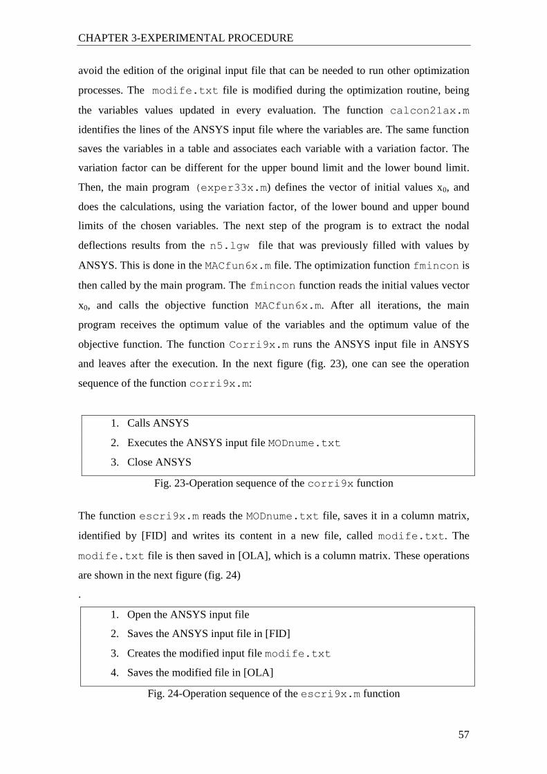
CHAPTER 3-EXPERIMENTAL PROCEDURE
57
avoid the edition of the original input file that can be needed to run other optimization
processes. The modife.txt file is modified during the optimization routine, being
the variables values updated in every evaluation. The function calcon21ax.m
identifies the lines of the ANSYS input file where the variables are. The same function
saves the variables in a table and associates each variable with a variation factor. The
variation factor can be different for the upper bound limit and the lower bound limit.
Then, the main program (exper33x.m) defines the vector of initial values x0, and
does the calculations, using the variation factor, of the lower bound and upper bound
limits of the chosen variables. The next step of the program is to extract the nodal
deflections results from the n5.lgw file that was previously filled with values by
ANSYS. This is done in the MACfun6x.m file. The optimization function fmincon is
then called by the main program. The fmincon function reads the initial values vector
x0, and calls the objective function MACfun6x.m. After all iterations, the main
program receives the optimum value of the variables and the optimum value of the
objective function. The function Corri9x.m runs the ANSYS input file in ANSYS
and leaves after the execution. In the next figure (fig. 23), one can see the operation
sequence of the function corri9x.m:
1. Calls ANSYS
2. Executes the ANSYS input file MODnume.txt
3. Close ANSYS
Fig. 23-Operation sequence of the corri9x function
The function escri9x.m reads the MODnume.txt file, saves it in a column matrix,
identified by [FID] and writes its content in a new file, called modife.txt. The
modife.txt file is then saved in [OLA], which is a column matrix. These operations
are shown in the next figure (fig. 24)
.
1. Open the ANSYS input file
2. Saves the ANSYS input file in [FID]
3. Creates the modified input file modife.txt
4. Saves the modified file in [OLA]
Fig. 24-Operation sequence of the escri9x.m function

CHAPTER 3-EXPERIMENTAL PROCEDURE
58
The function calcon21ax.m creates and fills the [PRN] and {PRNs} matrix. The
[PRN] and {PRNs} are matrix with the information necessary to inform the program the
value of the variables. In the next figure (fig. 25), one can see the operation sequence of
this function:
1. Create [PRN] and {PRNs} matrixes
2. Extract variables
3. Defines variable limits
4. Fills [PRN] and [PRNs]
Fig. 25-Operation sequence of the calcon21ax.m function
The MATLAB program builds a matrix denominated [PRN] which has five columns.
Each column has several lines, and the columns have, respectively:
1. The number of the line in the file where the parameter is located
2. The position where the equality signal is located
3. The value of the parameter
4 The lower bound limit
5 The upper bound limit
The program also builds a second table [PRNs], with one column containing a text
string with the parameter description in text. The function escrimx3.m reads the
modife.txt file, saves it in a column matrix identified by [OLAM] and changes the
lines corresponding to the variables, according with the information received in the
optimization routine. This information is received by a column matrix denominated
[PRNx]. The next figure (fig. 26) shows the operation sequence.
1. Reads the input file modife.txt
2. Modifies the [OLAM] matrix using the [PRNx] values
3. Saves the input file in [OLAM]
Fig. 26-Operation sequence of the escrimx3.m function
The function nlcOUT6x.m runs escrimx3.m and runs the modife.txt in
ANSYS, as shown in the figure below (fig. 27)
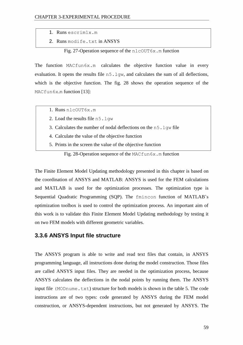
CHAPTER 3-EXPERIMENTAL PROCEDURE
59
1. Runs escrim1x.m
2. Runs modife.txt in ANSYS
Fig. 27-Operation sequence of the nlcOUT6x.m function
The function MACfun6x.m calculates the objective function value in every
evaluation. It opens the results file n5.lgw, and calculates the sum of all deflections,
which is the objective function. The fig. 28 shows the operation sequence of the
MACfun6x.m function [13]:
1. Runs nlcOUT6x.m
2. Load the results file n5.lgw
3. Calculates the number of nodal deflections on the n5.lgw file
4. Calculate the value of the objective function
5. Prints in the screen the value of the objective function
Fig. 28-Operation sequence of the MACfun6x.m function
The Finite Element Model Updating methodology presented in this chapter is based on
the coordination of ANSYS and MATLAB: ANSYS is used for the FEM calculations
and MATLAB is used for the optimization processes. The optimization type is
Sequential Quadratic Programming (SQP). The fmincon function of MATLAB’s
optimization toolbox is used to control the optimization process. An important aim of
this work is to validate this Finite Element Model Updating methodology by testing it
on two FEM models with different geometric variables.
3.3.6 ANSYS Input file structure
The ANSYS program is able to write and read text files that contain, in ANSYS
programming language, all instructions done during the model construction. Those files
are called ANSYS input files. They are needed in the optimization process, because
ANSYS calculates the deflections in the nodal points by running them. The ANSYS
input file (MODnume.txt) structure for both models is shown in the table 5. The code
instructions are of two types: code generated by ANSYS during the FEM model
construction, or ANSYS-dependent instructions, but not generated by ANSYS. The

CHAPTER 3-EXPERIMENTAL PROCEDURE
60
write of results to output file, the definition of initial variable values, the keypoints
coordinate modification in order to include the variables, and the commands to get
nodal deflections are the ANSYS-dependent instructions that were not originated during
the construction of the model.
User instruction Defines initial variable values
ANSYS-Preprocessor-Modeling
Creates Keypoints (with variables)
Creates Lines
Creates Areas
ANSYS-Preprocessor-Element type Select element type- Shell63
ANSYS-Preprocessor-Real constants Defines shell thickness
ANSYS-Preprocessor- Material
properties
Define Material properties
ANSYS-Preprocessor- Mesh tool Creates mesh
ANSYS-Solution- Loads Apply Loads and Displacements
ANSYS-Solution Solves the Model
User instruction Get nodal deflections from the model
User instruction Writes results to output file n5.lgw
Table 5-Sequence of the ANSYS input files operations.
The ANSYS input file code for the ribbed plate and tubular beam models is shown on
the Annex 3- Finite Element Model files.

61
CHAPTER 4-RESULTS

62
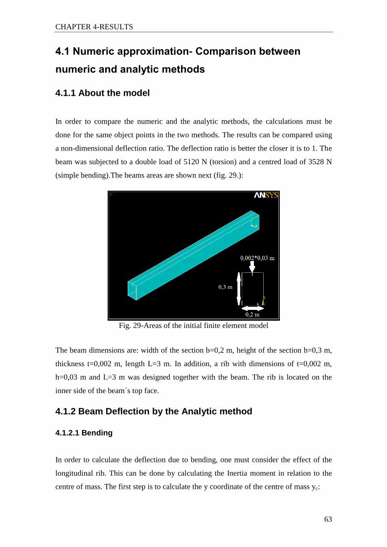
CHAPTER 4-RESULTS
63
4.1 Numeric approximation- Comparison between
numeric and analytic methods
4.1.1 About the model
In order to compare the numeric and the analytic methods, the calculations must be
done for the same object points in the two methods. The results can be compared using
a non-dimensional deflection ratio. The deflection ratio is better the closer it is to 1. The
beam was subjected to a double load of 5120 N (torsion) and a centred load of 3528 N
(simple bending).The beams areas are shown next (fig. 29.):
Fig. 29-Areas of the initial finite element model
The beam dimensions are: width of the section b=0,2 m, height of the section h=0,3 m,
thickness t=0,002 m, length L=3 m. In addition, a rib with dimensions of t=0,002 m,
h=0,03 m and L=3 m was designed together with the beam. The rib is located on the
inner side of the beam´s top face.
4.1.2 Beam Deflection by the Analytic method
4.1.2.1 Bending
In order to calculate the deflection due to bending, one must consider the effect of the
longitudinal rib. This can be done by calculating the Inertia moment in relation to the
centre of mass. The first step is to calculate the y coordinate of the centre of mass yc:

CHAPTER 4-RESULTS
64
1 1 2 2
c
1 2
m y +m y 2*0,285+47*0,15y = = =0,1556
m +m 2+47 m
where:
yc is the centre of mass coordinate of the system
m1 is the mass of the object 1(rib)
m2 is the mass of the object 2 (beam without rib)
y1 is the mean y coordinate of the object 1(rib)
y2 is the mean y coordinate of the object 2 (beam without rib)
The inertia moment of the object in relation to the x axis is:
3 3 3 3
1 1 -5xx
bh b h 0,2*0,3 0,196*0,296I = - = - *=2,64*10
12 12 12 12m
4
where:
Ixx is the inertia moment in relation to the x axis
b is the section width of the beam
h is the section height of the beam
b1 is the inner section width
h1 is the inner section height
The inertia moment in relation to the centre of mass can now be obtained:
2 -5 2 -5 4m xx cI =I +Ay =2,64*10 +0,002*0,03*0,1556 =2,7853*10 m
where:
Im is the inertia moment in relation to the centre of mass
A is the transversal rib area
The deflection due to bending can now be calculated using the calculated inertia
moment:
3 2 3 3 2 3
b2 3 9 -5 2 3
FL x x 3528*3 1,5 1,5y = 3 -4 = 3* -4*
48EI L L 48*210*10 *2,7853*10 3 3
58,482*10 m
4.1.2.2 Torsion
In torsion, the rigidity is governed by the transversal elasticity modulus G:

CHAPTER 4-RESULTS
65
910E 210*10
G= = =8,14*102*(1+ν) 2*(1+0,29)
Pa
The torsion moment can be calculated by multiplying the applied load P by the distance
between the line of action of the two binary forces. In this case the distance between the
line of action of the two binary forces bi is equal to the section width b. The torsion
moment is then:
tM=P*b=5120*0,2=1024 N.m
The area of the mean line is necessary to calculate the distortion angle :
2
0A =(b-e)*(h-e)=(0,2-0,002)*(0,3-0,002)=0,059 m
The shear stresses must be calculated, in order to be possible to calculate the shear flux:
0
Mt 1024τ= = =4338983,1 Pa
2*e*A 2*0,002*0,059
The shear flux can now be calculated, by multiplying the shear stress by the thickness of
the object:
C=τ*t=4338983,1*0,002=8678 Pa.m
The mean line perimeter lt must be calculated, in order to be possible to calculate the
distortion angle:
tl=2*((h-e)+(b-e))=2*((0,3-0,002)+(0,2-0,002))=0,992 m
The distortion angle can now be calculated:
t -4
100
Cl 8678*0,992θ= = =4,48*10 rad
2GA e 2*8,14*10 *0,059*0,002
To be possible to calculate the deflection due to torsion, one must calculate the diagonal
length of the object. It is necessary to calculate the angle of the section:
0,5*b 0,1
Tg = =0,5*h 0,15
-1 0,1=Τg ( )=33,7 º
0,15

CHAPTER 4-RESULTS
66
The length of the diagonal can then be calculated:
h 0,3
D= = =0,430 mcos cos33,7
The deflection due to torsion can now be calculated by multiplying half of the section
diagonal by the distortion angle and by the length:
-4 -4t
D 0,430y= θL= *4,48*10 *3=2,89*10 m
2 2
Because the rib is longitudinal, it has not a significant effect on the torsion deflection.
As a simplification, the rib was not considered in the calculation of the torsion
deflection yt.
4.1.2.3 Total deflection
The total deflection can be expressed as the sum of the torsion and bending deflections:
-5 -4 -4total b ty =y +y=8,482*10 +2,89*10 =3,74*10 m
4.1.3 Beam Deflection by the numeric method
The element type used in the initial beam is the shell elastic four nodes, named shell63.
The constraints were applied on the two lower keypoints in each side of the beam (four
in total), which means that the beam is simply supported as its ends. The total deflection
results are shown next (fig. 30):
Fig. 30-Deflection results for the initial FEM model

CHAPTER 4-RESULTS
67
One can see that the value obtained for the total deflection by the analytic method
belongs to the interval of values obtained by the numeric method. One can also see that
there is a much higher deflection in the central region of the beam, due to the applied
loads.
4.1.4 Comparison of numeric and analytic methods
As told before, the comparison between analytic and numeric methods was done using a
deflection ratio. The next figure (fig. 31) shows the points were deflections were
queried on the numeric method (on ANSYS).
Fig. 31- Points were results were queried on ANSYS
One can see that the results were queried on the top surface of the object, having the
points x coordinate of 0,1, y coordinate of 0,3 and z coordinate shown in fig. 31. In the
next table (table 6) one can see the deflection results by the two methods. The deflection
ratio was calculated and is also shown on the same table:

CHAPTER 4-RESULTS
68
Analytic Numeric
Z coordinate[m] yb [m] yt [m] ytotal [m] Total
deflection[m]
Deflection
ratio
0 0,00E+00 2,89E-04 2,89E-04 2,50E-04 1,16
0,3 8,82E-06 2,89E-04 2,98E-04 2,60E-04 1,15
0,6 2,98E-05 2,89E-04 3,19E-04 2,77E-04 1,15
0,9 5,49E-05 2,89E-04 3,44E-04 2,50E-04 1,38
1,2 7,60E-05 2,89E-04 3,65E-04 8,99E-05 4,06
1,5 8,48E-05 2,89E-04 3,74E-04 1,32E-03 0,28
1,8 7,60E-05 2,89E-04 3,65E-04 8,99E-05 4,06
2,1 5,49E-05 2,89E-04 3,44E-04 2,50E-04 1,38
2,4 2,98E-05 2,89E-04 3,19E-04 2,77E-04 1,15
2,7 8,82E-06 2,89E-04 2,98E-04 2,60E-04 1,15
3 0,00E+00 2,89E-04 2,89E-04 2,50E-04 1,16
Table 6-Comparison between numeric and analytic method in terms of strain
The bending deflection is a function of the distance to the supports, and the deflection
due to torsion is constant. In the next figure (fig. 32), one can see the deflection ratio for
the analytic and numeric methods. The deflection ratio is better, the closer it is to 1.
Fig. 32-Deflection Ratio in function of the z coordinate
0,00
0,50
1,00
1,50
2,00
2,50
3,00
3,50
4,00
4,50
0 0,3 0,6 0,9 1,2 1,5 1,8 2,1 2,4 2,7 3
De
fle
ctio
n r
atio
Z coordinate (m)
CHAPTER 4-RESULTS
69
The deflection ratio is close to 1 for most of the considered points, except for the center
point and for the two points near center. The low deflection ratio in the center of the
beam is due to stress concentration in the numeric method, because one load is
concentrated and applied in the center of the beam. Because there is stress concentration
in the center of the object, it is normal that there is less stress in the surrounding zones.
This fact can explain the high stress ratios in the points z=1,2 and z=1,8. One can also
see that the deflection ratio results are symmetric (fig. 32).
4.2 Mechanical Tests
In the chapter 3, the selected material was the DOCOL dual-phase steel. However, there
is no Young modulus or Poisson coefficient value in the DOCOL dual-phase steels
catalogue. Also, there is a range of values for the Yield stress. Because the lack of
material properties values in the catalogue, there is the need to perform mechanical tests
to determine a value for the Young modulus, Poisson coefficient and Yield stress. The
mechanical tests performed were two: tensile test and extensometry test. The tensile test
has the aim of determining Yield stress with 0,2% offset and Young modulus. The
extensometry test has the aim of determining Poisson coefficient, and was also used to
determine Young modulus. Because in tensile test the material suffers rupture, both the
elastic and plastic domains can be studied. The Yield stress was determined only in
tensile test, because in extensometry test the material is always in the elastic domain.
The Young modulus can be determined in both tensile and extensometry tests. In tensile
test, one considers the Stress-Strain chart and selects only the points that belong to the
elastic domain. By using a linear fit, one can obtain the Young modulus, because of the
proportionality between the stresses and strains in the elastic domain. In extensometry
test, one determines the stress by dividing the load by the transversal area of the
specimen. Then, dividing the obtained Stress by the longitudinal strain, one can obtain
the Young modulus. The Poisson coefficient is determined in extensometry test by
applying relatively small loads, and measuring the longitudinal and transversal strain
using an extensometer. The Poisson coefficient is the ratio between the transversal and
longitudinal strain.
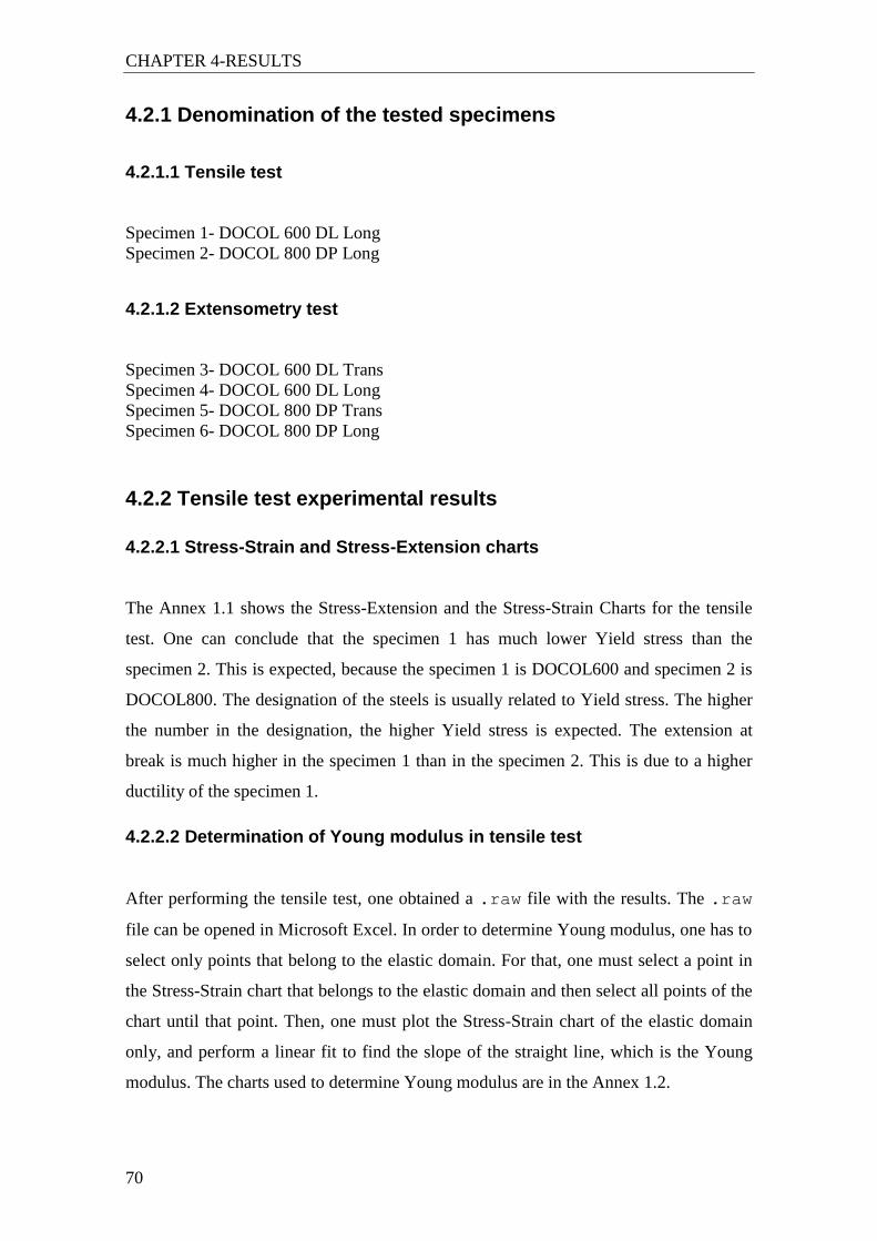
CHAPTER 4-RESULTS
70
4.2.1 Denomination of the tested specimens
4.2.1.1 Tensile test
Specimen 1- DOCOL 600 DL Long
Specimen 2- DOCOL 800 DP Long
4.2.1.2 Extensometry test
Specimen 3- DOCOL 600 DL Trans
Specimen 4- DOCOL 600 DL Long
Specimen 5- DOCOL 800 DP Trans
Specimen 6- DOCOL 800 DP Long
4.2.2 Tensile test experimental results
4.2.2.1 Stress-Strain and Stress-Extension charts
The Annex 1.1 shows the Stress-Extension and the Stress-Strain Charts for the tensile
test. One can conclude that the specimen 1 has much lower Yield stress than the
specimen 2. This is expected, because the specimen 1 is DOCOL600 and specimen 2 is
DOCOL800. The designation of the steels is usually related to Yield stress. The higher
the number in the designation, the higher Yield stress is expected. The extension at
break is much higher in the specimen 1 than in the specimen 2. This is due to a higher
ductility of the specimen 1.
4.2.2.2 Determination of Young modulus in tensile test
After performing the tensile test, one obtained a .raw file with the results. The .raw
file can be opened in Microsoft Excel. In order to determine Young modulus, one has to
select only points that belong to the elastic domain. For that, one must select a point in
the Stress-Strain chart that belongs to the elastic domain and then select all points of the
chart until that point. Then, one must plot the Stress-Strain chart of the elastic domain
only, and perform a linear fit to find the slope of the straight line, which is the Young
modulus. The charts used to determine Young modulus are in the Annex 1.2.
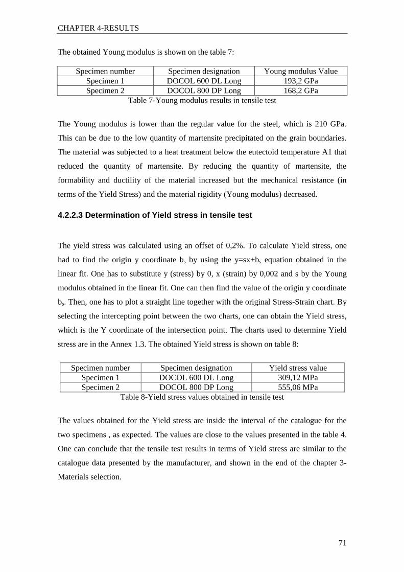
CHAPTER 4-RESULTS
71
The obtained Young modulus is shown on the table 7:
Specimen number Specimen designation Young modulus Value
Specimen 1 DOCOL 600 DL Long 193,2 GPa
Specimen 2 DOCOL 800 DP Long 168,2 GPa
Table 7-Young modulus results in tensile test
The Young modulus is lower than the regular value for the steel, which is 210 GPa.
This can be due to the low quantity of martensite precipitated on the grain boundaries.
The material was subjected to a heat treatment below the eutectoid temperature A1 that
reduced the quantity of martensite. By reducing the quantity of martensite, the
formability and ductility of the material increased but the mechanical resistance (in
terms of the Yield Stress) and the material rigidity (Young modulus) decreased.
4.2.2.3 Determination of Yield stress in tensile test
The yield stress was calculated using an offset of 0,2%. To calculate Yield stress, one
had to find the origin y coordinate bs by using the y=sx+bs equation obtained in the
linear fit. One has to substitute y (stress) by 0, x (strain) by 0,002 and s by the Young
modulus obtained in the linear fit. One can then find the value of the origin y coordinate
bs. Then, one has to plot a straight line together with the original Stress-Strain chart. By
selecting the intercepting point between the two charts, one can obtain the Yield stress,
which is the Y coordinate of the intersection point. The charts used to determine Yield
stress are in the Annex 1.3. The obtained Yield stress is shown on table 8:
Specimen number Specimen designation Yield stress value
Specimen 1 DOCOL 600 DL Long 309,12 MPa
Specimen 2 DOCOL 800 DP Long 555,06 MPa
Table 8-Yield stress values obtained in tensile test
The values obtained for the Yield stress are inside the interval of the catalogue for the
two specimens , as expected. The values are close to the values presented in the table 4.
One can conclude that the tensile test results in terms of Yield stress are similar to the
catalogue data presented by the manufacturer, and shown in the end of the chapter 3-
Materials selection.
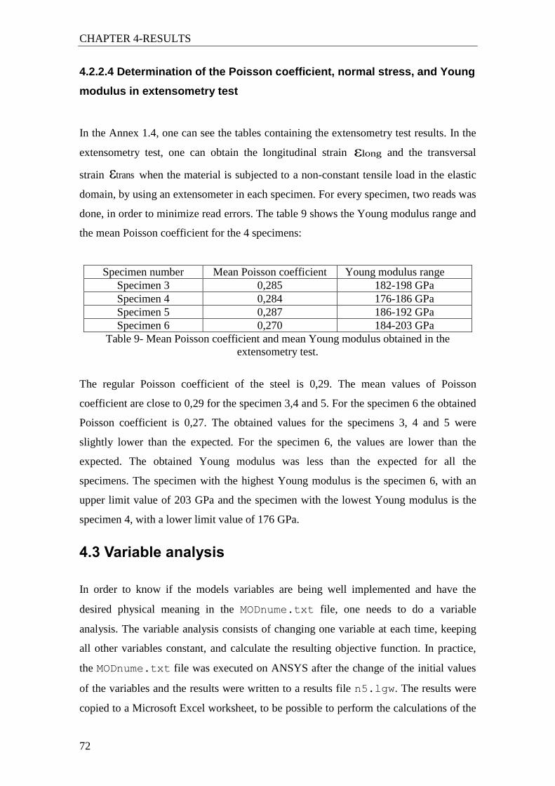
CHAPTER 4-RESULTS
72
4.2.2.4 Determination of the Poisson coefficient, normal stress, and Young
modulus in extensometry test
In the Annex 1.4, one can see the tables containing the extensometry test results. In the
extensometry test, one can obtain the longitudinal strain long ε and the transversal
strain transε when the material is subjected to a non-constant tensile load in the elastic
domain, by using an extensometer in each specimen. For every specimen, two reads was
done, in order to minimize read errors. The table 9 shows the Young modulus range and
the mean Poisson coefficient for the 4 specimens:
Specimen number Mean Poisson coefficient Young modulus range
Specimen 3 0,285 182-198 GPa
Specimen 4 0,284 176-186 GPa
Specimen 5 0,287 186-192 GPa
Specimen 6 0,270 184-203 GPa
Table 9- Mean Poisson coefficient and mean Young modulus obtained in the
extensometry test.
The regular Poisson coefficient of the steel is 0,29. The mean values of Poisson
coefficient are close to 0,29 for the specimen 3,4 and 5. For the specimen 6 the obtained
Poisson coefficient is 0,27. The obtained values for the specimens 3, 4 and 5 were
slightly lower than the expected. For the specimen 6, the values are lower than the
expected. The obtained Young modulus was less than the expected for all the
specimens. The specimen with the highest Young modulus is the specimen 6, with an
upper limit value of 203 GPa and the specimen with the lowest Young modulus is the
specimen 4, with a lower limit value of 176 GPa.
4.3 Variable analysis
In order to know if the models variables are being well implemented and have the
desired physical meaning in the MODnume.txt file, one needs to do a variable
analysis. The variable analysis consists of changing one variable at each time, keeping
all other variables constant, and calculate the resulting objective function. In practice,
the MODnume.txt file was executed on ANSYS after the change of the initial values
of the variables and the results were written to a results file n5.lgw. The results were
copied to a Microsoft Excel worksheet, to be possible to perform the calculations of the

CHAPTER 4-RESULTS
73
objective function. This type of analysis was done for the two models: the ribbed plate,
and the tubular beam. The optimization variables are subjected to constraints limits
b 0 bl x u
where:
lb is the lower bound
x0 is the initial value
ub is the upper bound
The limits are different for the geometric variables in the two models, since its initial
value is also different. The vector x0 is the initial values vector (line vector). The
variable names start in PR(PRLG1,PRLG2,PRLG3,PREX,etc.), however, in the
optimization there is the need that the initial variables values are all of the same order
(for example, in the geometric parameters optimization if PRLG1 has a value of 0,2 ,
then PRLG2 and PRLG3 value must belong to the interval [0,1;1[ ). This detail is for
the MATLAB optimization program to deal with all variables in the same order of
value. Having that fact in consideration, one must define a relation between the PR
variables, and the variables used by the program, because the initial variable values
have a different order of value. A relation variable has the same name as the original,
but without the PR (PRLG1 relation variable is denoted by LG1, PREX has a relation
variable of EX, and so on). The variable analysis can be useful to determine the
importance of each variable in the optimization program, but it can also be used to have
a rough idea if the variables are being well written in the ANSYS input file. For
example, if the objective function decreases with the decrease of the LG3 variable “rib
thickness”, then something is wrong in the ANSYS input file. A decrease of the PRLG3
variable must originate a worse (higher) objective function. In the Annex 2.1, one can
see the deflection results for each considered nodal point, when one variable value
changes. The variable values are also shown on each table. The objective function was
calculated by the sum of the absolute values of the deflections in all considered nodal
points. The objective function values were used to make one chart per each variable per
model, representing the variation of the objective function as dependent variable with
the value of each considered variable as independent variable.
CHAPTER 4-RESULTS
74
4.3.1 Variable analysis of model 1- ribbed plate
About the variable analysis of model 1, one can say that the variation of the three
material properties variables seems to be logical: the objective function decreases
linearly with the increase of Young modulus. The higher the Young modulus, the higher
rigidity the material has, and, as a consequence, the lower are the deflections. About
Poisson coefficient, one can say that an increase of the Poisson coefficient leads to
lower deflections. This happens because the higher the Poisson coefficient, the higher is
the transversal deformation in relation to the longitudinal deformation. Because there is
less longitudinal deformation the resulting deflections are lower. The density does not
affect in any way the objective function, being the objective function totally
independent of the density value. About the LG1 variable, the results are not so logical.
There is a decrease of the objective function value from LG1=0,01 m to LG1=0,025 m
and then a sudden increase from LG1=0,025 m to LG1=0,03 m. This could happen due
to the small number of considered nodes (15) used to calculate the objective function. In
fact, one can see that the nodes 7 and 8 in the model 1 for LG1=0,03 have much higher
deflection than for LG1=0,025. If the number of considered nodes was higher, ideally
all nodes, the expected results were a decrease of the objective function with a decrease
of the LG1 variable. About LG2, one can say that the objective function decreases with
the increasing value of the rib height, except for LG2=0,65. This can be due to the small
number of nodal points considered for the calculations that can lead to a high error in
results, as for the LG1 variable. The variation of the LG3 variable, which is the
thickness, seems to be logical: the higher the thickness, the lower is the objective
function, in an approximate inverse proportionality. In the Annex 2 one can see the
variable analysis tables and charts for this model.
4.3.2 Variable analysis of model 2- tubular beam
About the variable analysis of Model 2, one can say that the material properties have an
expected influence on the objective function, like in the model 1. The LG4 variable has
an expected behavior, because the higher the distance of the center to the corner
segment of the cross section, the lower rigidity the object has. As a consequence, the
objective function is higher. The LG5 variable has a non-linear behavior, which could
happen due to the self non-linearity of the variable, or due to the small number of

CHAPTER 4-RESULTS
75
considered nodes, like in the LG1 and LG2 variables of the ribbed plate model. The
LG6 variable has an expected influence on the objective function: the higher the LG6
variable, the higher the object rigidity, and, as a consequence, the objective function is
lower. In the Annex 2, one can see the variable analysis tables and charts for the tubular
beam model.
4.4 Optimization results
The ANSYS input file MODnume.txt is used by MATLAB and ANSYS in the
optimization routines and the modifications that occur during the optimization processes
are written to another file called modife.txt. First, the three geometric variables
were optimized. Then the three material properties were optimized. Then one uses the
optimized variables values of both geometric parameters optimization and material
properties optimization and runs an optimization with all six variables. The results were
analyzed in terms of optimization, having in consideration the initial variable values, the
final variable values and the final value of the objective function in each optimization
routine for both models, but also in terms of the FEM results, which are useful to show
that the models deflections decreased in a global way, and not only on the considered
nodal points.
4.4.1 Model 1-Ribbed plate
4.4.1.1 Initial variable values and limits
The initial variable values and the variable limits for the geometric parameters
optimization were: (Table 10):
Variable Lower Bound Initial Value Upper Bound
LG1[m] 0,025 0,100 0,230
LG2[m] 0,0075 0,030 0,069
LG3[m] 0,0005 0,002 0,0046
Table 10-Variable limits for the geometric optimization (ribbed plate)
The initial values and the limits for the material properties optimization were: (table 11)
Variable Lower Bound Initial Value Upper Bound
EX[GPa] 21 210 231
PXY 0,145 0,29 0,435
DNS[kg/m3] 3945 7890 15780

CHAPTER 4-RESULTS
76
Table 11-Variable limits for the material properties optimization (ribbed plate)
For all variables optimization, the initial variable values and the variable limits were:
(table 12):
Variable Lower Bound Initial Value Upper Bound
LG1[m] 0,00625 0,025 0,0575
LG2[m] 0,01275 0,0510 0,11730
LG3[m] 0,001150 0,0046 0,010580
EX [GPa] 23,1 231 254,1
PXY 0,2175 0,435 0,6525
DNS[kg/m3] 3945 7890 15780
Table 12-Variable limits for all variables optimization (tubular beam)
4.4.1.2 Geometric parameters optimization results
The final value of the objective function is: q(x)=0,00092 m
The optimum design variables are (table 13):
Variable Value
LG1[m] 0,025
LG2[m] 0,0510
LG3[m] 0,0046
Table 13-Final variable values for the geometric parameters optimization (ribbed plate)
The final value of the LG1 variable is the lower limit. In the LG1 variable analysis one
can see that the minimum objective function is obtained when LG1=0,025 m, which is
the final LG1 variable value. The optimum value of the LG2 variable is closer to the
upper bound than to the lower bound, as expected. The optimum value of LG3 is the
upper bound. The LG3 variable behavior can be understood by looking at the variable
analysis, where one can see that the objective function always decreases with an
increasing value of LG3 variable, which means that the optimum value is always the
upper bound. With that fact in consideration, there is no need to change the variable
limits.
4.4.1.3 Material properties optimization results
The final value of the objective function is: q(x)=0,04258 m
The optimum design variables are: (table 14)

CHAPTER 4-RESULTS
77
Variable Value
EX [GPa] 231
PXY 0,435
DNS[kg/m3] 7890
Table 14-Final variable values for the material properties optimization (ribbed plate)
The final variables values for the EX and PXY variables are the upper bound limits. In
fact, the variable analysis showed that the value of the objective function always
decreases with an increase of the EX and PXY variables values. The density has no
influence on the objective function, as demonstrated in the variable analysis.
4.4.1.4 Optimization results using all variables
The final value of the objective function is: q(x)=0,00077 m
The optimum design variables are (table 15):
Variable Value
LG1[m] 0,025
LG2[m] 0,051
LG3[m] 0,0046
EX [GPa] 231
PXY 0,435
DNS[kg/m3] 7890
Table 15-Final variable values for all variables optimization (ribbed plate)
One can say that the results are quite similar to the obtained before in the materials
properties optimization and in the geometric parameters optimization. This means that
the MATLAB optimization program is not able to further optimize the models. This can
be due to already fully optimized values or the function tolerance is not sufficiently low,
and therefore MATLAB has no resolution to further optimize the models.
4.4.2 Model 2- Tubular beam
4.4.2.1 Initial variable values and limits
For the geometric parameters optimization, the initial variable values and the variable
limits were (table 16):

CHAPTER 4-RESULTS
78
Variable Lower Bound Initial Value Upper Bound
LG4[m] 0,0213 0,0850 0,1955
LG5[m] 0,0075 0,0300 0,0690
LG6[m] 0,0088 0,0350 0,0805
Table 16-Variable limits for the geometric parameters optimization (tubular beam)
For the material properties optimization, the initial variable values and variable limits
were (table 17):
Variable Lower Bound Initial Value Upper Bound
EX [GPa] 21 210 231
PXY 0,145 0,29 0,435
DNS[kg/m3] 3945 7890 15780
Table 17-Variable limits for the material properties optimization (tubular beam)
For all variables optimization, the initial variable values and the variable limits were
(table 18):
Variable Lower Bound Initial Value Upper Bound
LG4[m] 0,00531 0,0213 0,04888
LG5[m] 0,001905 0,0076 0,017526
LG6[m] 0,02013 0,0805 0,18515
EX [GPa] 23,1 231 254,1
PXY 0,1460 0,2919 0,4378
DNS[kg/m3] 3945 7890 15780
Table 18-Variable limits for all variables optimization (tubular beam)
4.4.2.2 Geometric parameters optimization results
The final value of the objective function is: q(x)=0,00053 m
The optimum design variables are presented in table 19:
Variable Value
LG4[m] 0,0213
LG5[m] 0,0076
LG6[m] 0,0805
Table 19-Final variable values for the geometric optimization
One can say that the optimum value for the LG4 variable is the lower bound. In fact, in
the variable analysis charts (Annex 2.2) one can see that the objective function always
increase with the increase of the LG4 variable. If the variable limits were changed, the
optimum value would be always the lower bound. If the lower bound had a lower value,
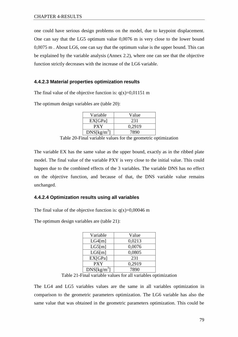
CHAPTER 4-RESULTS
79
one could have serious design problems on the model, due to keypoint displacement.
One can say that the LG5 optimum value 0,0076 m is very close to the lower bound
0,0075 m . About LG6, one can say that the optimum value is the upper bound. This can
be explained by the variable analysis (Annex 2.2), where one can see that the objective
function strictly decreases with the increase of the LG6 variable.
4.4.2.3 Material properties optimization results
The final value of the objective function is: q(x)=0,01151 m
The optimum design variables are (table 20):
Variable Value
EX[GPa] 231
PXY 0,2919
DNS[kg/m3] 7890
Table 20-Final variable values for the geometric optimization
The variable EX has the same value as the upper bound, exactly as in the ribbed plate
model. The final value of the variable PXY is very close to the initial value. This could
happen due to the combined effects of the 3 variables. The variable DNS has no effect
on the objective function, and because of that, the DNS variable value remains
unchanged.
4.4.2.4 Optimization results using all variables
The final value of the objective function is: q(x)=0,00046 m
The optimum design variables are (table 21):
Variable Value
LG4[m] 0,0213
LG5[m] 0,0076
LG6[m] 0,0805
EX[GPa] 231
PXY 0,2919
DNS[kg/m3] 7890
Table 21-Final variable values for all variables optimization
The LG4 and LG5 variables values are the same in all variables optimization in
comparison to the geometric parameters optimization. The LG6 variable has also the
same value that was obtained in the geometric parameters optimization. This could be

CHAPTER 4-RESULTS
80
due to the value of the function tolerance (10-6
), which allows relatively fast results
processing time, but with a loss of resolution in the optimization process. The optimized
values of the material properties are the same than the obtained in the previous materials
optimization routine: the density did not change because, as told before, the objective
function value does not depend of it, and the Young modulus and Poisson coefficient
remain unchanged because they already have the optimum value for the used function
tolerance.
4.5 Optimization settings
The optimization settings were the following:
'MaxFunEvals'=300
'MaxIter',=200
'DiffMaxChange'=10
'DiffMinChange'=1*10-1
'TolFun'=1*10-6
where:
MaxFunEvals is the maximum evaluations that can be run on a single iteration
MaxIter is the maximum number of iterations allowed in the optimization process.
DiffMaxChange is the maximum value that a variable can change at once
DiffMinChange is the minimum value that a variable can change at once
TolFun is the function tolerance
In every optimization routine done in this work, the optimization ended with the
following message: “Local minimum found that satisfies the constraints. Optimization
completed because the objective function is non-decreasing in feasible directions, to
within the selected value of the function tolerance, and constraints were satisfied to
within the default value of the constraint tolerance.”
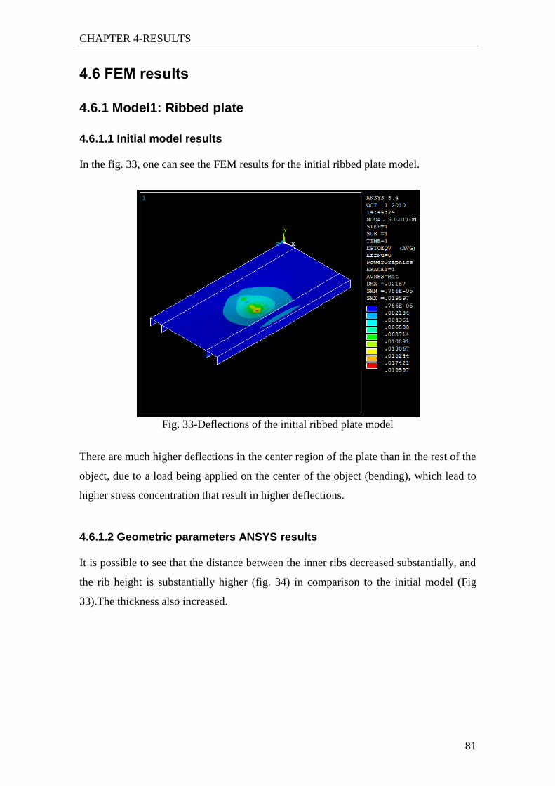
CHAPTER 4-RESULTS
81
4.6 FEM results
4.6.1 Model1: Ribbed plate
4.6.1.1 Initial model results
In the fig. 33, one can see the FEM results for the initial ribbed plate model.
Fig. 33-Deflections of the initial ribbed plate model
There are much higher deflections in the center region of the plate than in the rest of the
object, due to a load being applied on the center of the object (bending), which lead to
higher stress concentration that result in higher deflections.
4.6.1.2 Geometric parameters ANSYS results It is possible to see that the distance between the inner ribs decreased substantially, and
the rib height is substantially higher (fig. 34) in comparison to the initial model (Fig
33).The thickness also increased.

CHAPTER 4-RESULTS
82
Fig. 34-Deflections of the ribbed plate model after geometric parameters optimization
Because the element type is shell, it is not possible to know by the screenshot if the
thickness is lower or higher in comparison to the initial model, it is only possible to
know by the optimization results. The deflections reduced greatly in comparison to the
initial model: the maximum deflection decreased from 0,019597 m to 0,003748 m,
which is great. The minimum deflection decreased from 0,786*10-5
m to 0,331*10-5
m,
which means that the minimum deflection of the optimized model is near half of the
initial model.
4.6.1.3 Material properties ANSYS results
The deflection results of the material properties optimization seem to be higher (fig. 35)
than the initial model (fig. 33).
Fig. 35-Deflections of the ribbed plate model after material properties optimization

CHAPTER 4-RESULTS
83
This was surely true if the colors of the two figures were exactly the same. One can see
that there is a higher quantity of dark blue in the fig. 35, which means that the deflection
in that area reduced. In fact, the dark blue deflection range in the fig. 35 is [0,947*10-5
,
2,467*10-3
] m and the blue deflection in the fig. 33 is [2,184*10-3
-4,361*10-3
] m, which
means there is a deflection reduction. The nodes with deflection higher than 2,184*10-3
m in the fig. 35 can have a higher deflection than in the fig. 33, but in general terms,
there is a deflection reduction.
4.6.1.4 ANSYS results using all variables
The FEM results of all variables optimization show that the deflections have decreased
strongly (fig. 36) in comparison to the initial model (fig. 33).
Fig. 36-Deflections of the ribbed plate model after all variables optimization
There is a larger area of dark blue, which means that the deflections have reduced in
that area. When comparing the deflection value range of each color, one can see that
there is a strong decrease of the deflections for all colors.
4.6.2 Model2: Tubular beam
4.6.2.1 Initial model results
The initial tubular beam model is represented on the next figure (fig. 37).

CHAPTER 4-RESULTS
84
Fig. 37-Nodal deflection for the initial tubular beam model
In fig. 37 one can see the nodal deflections of the initial tubular beam model. Like in the
ribbed plate model, one can see much higher deflections in the center region of the
object, because there is one load applied exactly in the center of the object (bending),
and there is also a binary load that is equivalent to a torsion moment. One can say that
the initial tubular beam model has low deflections, and has a good rigidity.
4.6.2.2 Geometric parameters ANSYS results
It is possible to see that the cross section shape of the tubular beam suffered a severe
change during the optimization (fig. 37 and fig. 38).
Fig. 38-Nodal deflections for the geometrically optimized tubular beam model
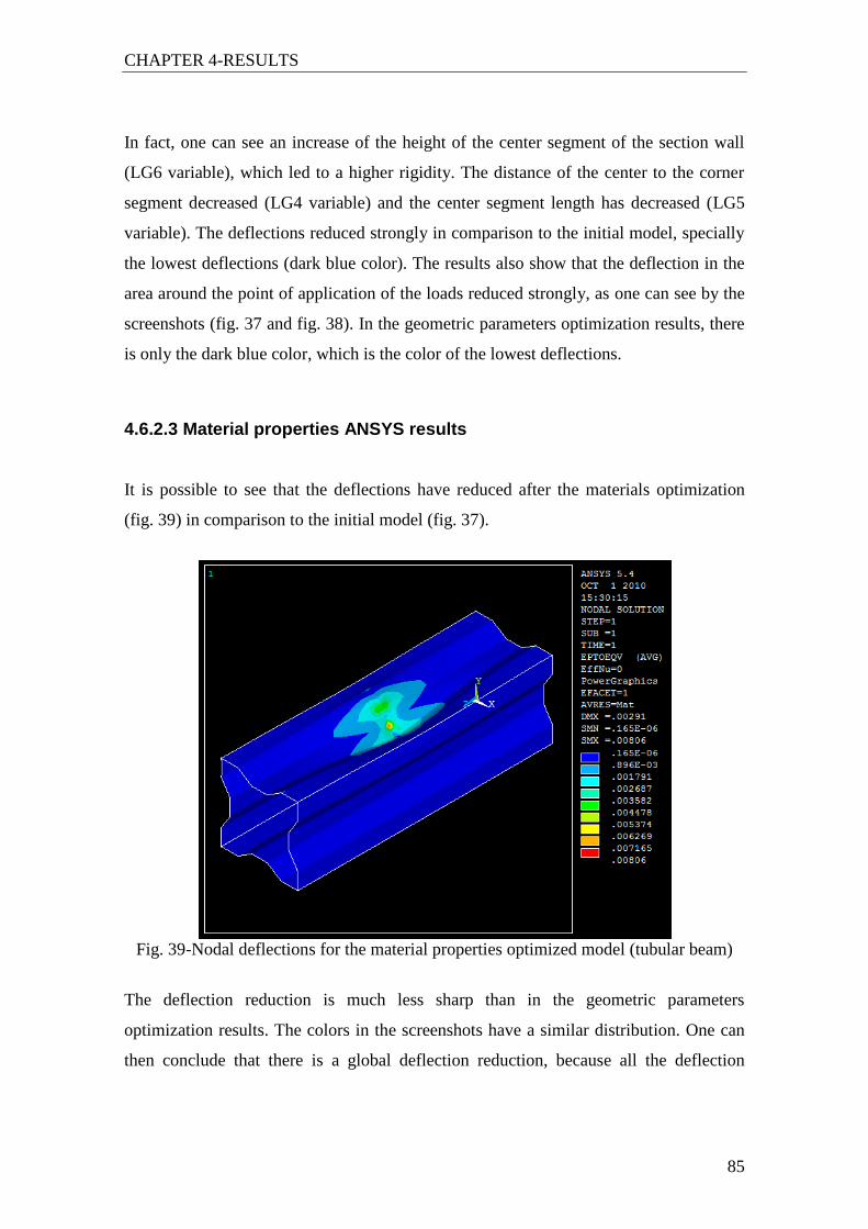
CHAPTER 4-RESULTS
85
In fact, one can see an increase of the height of the center segment of the section wall
(LG6 variable), which led to a higher rigidity. The distance of the center to the corner
segment decreased (LG4 variable) and the center segment length has decreased (LG5
variable). The deflections reduced strongly in comparison to the initial model, specially
the lowest deflections (dark blue color). The results also show that the deflection in the
area around the point of application of the loads reduced strongly, as one can see by the
screenshots (fig. 37 and fig. 38). In the geometric parameters optimization results, there
is only the dark blue color, which is the color of the lowest deflections.
4.6.2.3 Material properties ANSYS results
It is possible to see that the deflections have reduced after the materials optimization
(fig. 39) in comparison to the initial model (fig. 37).
Fig. 39-Nodal deflections for the material properties optimized model (tubular beam)
The deflection reduction is much less sharp than in the geometric parameters
optimization results. The colors in the screenshots have a similar distribution. One can
then conclude that there is a global deflection reduction, because all the deflection

CHAPTER 4-RESULTS
86
values are lower in the fig. 39 than in the fig. 37 and the color distribution in the two
screenshots is very similar.
4.6.2.4 ANSYS results using all variables
The FEM screenshots for all-variables optimization (fig. 40) show that the geometric
parameters values are quite similar than in the geometric parameters optimization, due
to the similar shape of the object cross section.
Fig. 40-Nodal deflections for all variables optimized model (tubular beam)
There is only one color in the fig. 40, which is dark blue. This means that the
deflections are very low in every zones of the model. All the deflection values are lower
than in the initial model. A huge decrease in the deflection can be seen in the lower
bound of dark blue color: 0,292*10-8
m in the optimized model (fig. 40) and 0,185*10-6
m in the initial model (fig. 37).

87
CHAPTER 5-RESULTS DISCUSSION AND
CONCLUSIONS

88
CHAPTER 5-RESULTS DISCUSSION AND CONCLUSIONS
89
5.1 Results discussion
5.1.1 Variable analysis
5.1.1.1Material properties
The variables EX, PXY, and DNS have the physical meaning of: Young modulus,
Poisson coefficient, and density, respectively. The variable analysis tables and charts are
on the Annex 2.1 and Annex 2.2, respectively. The variable analysis charts for those
variables have a similar curve for both models. One can see that there is a linear
dependency between the objective function and the Young modulus. The objective
function decreases with the increase of Young modulus. This behavior is expected,
because a higher material rigidity leads to higher object rigidity. There is an almost
linear dependency between the Poisson coefficient and the objective function. The
objective function decreases with the increase of the Poisson coefficient. This behavior
is expected, because when the longitudinal strain is higher and the transversal strain is
kept constant the Poisson coefficient decreases. The objective function is not dependent
of the density, as one can see by the results.
5.1.1.2 Geometric parameters
5.1.1.2.1 Model 1: ribbed plate
The chart q(x)=f(LG1) shows a non-linear dependency between the distance of the inner
ribs to the center (LG1 variable) and the objective function. One can see that the
minimum value of the objective function occurs for LG1=0,025 m. According to this
fact, the geometrically optimized model has a LG1 value of 0,025 m in order to
minimize the objective function. One can say that the objective function decreases with
LG2 from LG2=0,036 m to LG2=0,061 m. From LG2=0,061 m to LG2=0,066 m there
is a significant increase of the objective function. There is a decrease of the objective
function with an increase of the LG3 variable (thickness). The variation is similar to an
inverse proportionality. An increase of the LG3 variable will necessarily result in a
higher Inertia moment, and will originate a lower objective function q(x).

CHAPTER 5-RESULTS DISCUSSION AND CONCLUSIONS
90
5.1.1.2.2 Model 2: tubular beam
The objective function always increases with the increase of the LG4 variable in the
considered interval [0,015;0,027]. About LG5, the objective function suffers little
variation from the interval [0,005;0,01], and then decreases sharply for LG5=0,011. The
variable analysis chart is similar to an inverse proportionality for LG6 variable. In LG6
variable analysis chart, the objective function always decreases in the chosen interval
[0,066;0,096].
5.1.2 Mechanical tests
A great variety of materials were analyzed for this application. However, one can
conclude that the dual-phase steel is the most adequate material because: it has a high
Young modulus, despite not as high as expected, its cost is relatively low, and their
Yield stress is high, which means that the material has high mechanical resistance, and
can be subjected to high loads before entering the plastic domain. Because of these
reasons, dual-phase specimens were obtained and mechanically tested to determine the
most relevant properties for the application: Yield stress, Young modulus and Poisson
coefficient.
5.1.2.1 Extensometry test
The obtained Poisson coefficient was near 0,29, which is the normal value for a steel,
except for the specimen 6. For the specimen 6, the obtained Poisson coefficient was
near 0,27. The Young modulus obtained by the extensometry test ranged from near 180
to 200 GPa. Those values are lower than the regular value of the steel, which is 210
GPa.
5.1.2.2 Tensile test
The specimen 1 has the highest Young modulus of the two specimens tested: 193,2
GPa. The specimen 2 has a Young modulus of near 168,2 GPa, which is much lower
than the expected 210 GPa. The Specimen 1 has a lower Yield stress, which is expected,
because its designation is 600 and the designation of the specimen 2 is 800. This
number is related to the Yield stress in relative terms, which means that a lower number
CHAPTER 5-RESULTS DISCUSSION AND CONCLUSIONS
91
designation means a lower Yield stress when comparing two specimens. The Yield
stress was measured using a 0,2% proportionality straight line that is parallel to the
elastic domain of the stress-strain curve. The Yield stress can be determined by the
intersection of the stress-strain curve with the straight line.
5.1.3 Optimization results
The final variable values usually comply with the results of the variable analysis. When
this does not happen, it´s because the variables when studied alone have different
behavior then when studied in combination with others. The obtained objective function
is lower in the geometric parameters optimization than in the material properties
optimization for both models. One can then conclude that the optimization of the
geometry is more important than the optimization of the material to achieve deflection
reduction.
5.1.4 FEM results
One can say that sometimes is obvious the deflection decrease between optimized and
non-optimized models. In the other cases, mainly in the material properties optimized
models, the deflections may seem to increase. This is not true, because the material
properties optimization screenshots have a larger area of dark blue. So, some values
may be higher in the material optimized model screenshot, but there is a deflection
decrease in most of the nodes of the object.
What could have happened during this work is that the considered number of nodal
points in both models was small (15 nodal points in the ribbed plate model and 21 in the
tubular beam model), and due to that fact, there can be a high error when comparing the
FEM results with the optimization results.
5.1.5 Materials selection
The material selection charts made possible the material selection for the applications of
this work. The analysed charts were Young modulus/Cost and Young modulus/density.
The desirable properties are: highest possible Young modulus to improve material
stiffness, lowest possible Cost for the solution to be reliable and lowest possible density
for the improvement of the admissible acceleration, having in mind that a lower density
CHAPTER 5-RESULTS DISCUSSION AND CONCLUSIONS
92
means a lower mass for objects with the same dimensions. The combination of those
factors dictates the best material. It was found that the best material is the high-strength
steel. The specific material is the DOCOL dual-phase steel.
5.2 Conclusions of the work
The conclusions of this work are:
- The Finite Element Model Updating code developed in this work can be successfully
used to optimize both geometric parameters and material properties.
- The geometric parameters play a more important role in the optimization process than
the material properties, because the obtained objective function is lower in the
geometric parameters optimization than in the material properties optimization.
- The DOCOL dual phase steels tested by tensile test and extensometry test have a
lower Young modulus than the expected. The expected value was 210 GPa.
- The Young modulus and the Poisson coefficient are relevant properties for the
deflection reduction, because they have influence on the objective function, as shown on
the variable analysis.
- The density has no influence on the objective function.
- The material properties influence on the objective function is the same for the two
models studied in this work. However, the value of the objective function was not the
same, because the objects are of different nature.
- The tested materials have high Yield stresses, which mean that the material can be
subjected to high loads before entering the plastic domain. In the practical applications
of this work (plotters and laser cutting machines) it is very important to ensure that the
material doesn´t reach the plastic domain, otherwise the permanent deformation will
negatively affect the machine operation. Considering this fact, the dual phase steels are
an adequate material for the applications of this work.
5.3 Future work proposals
A graphical interface could be created in order to implement the Finite Element Model
Updating code developed in this work in a user-friendly environment. The
programming code could then be used to create an executable file, in order to avoid the

CHAPTER 5-RESULTS DISCUSSION AND CONCLUSIONS
93
need of having MATLAB installed on the computer. Other models can be tested by this
novel methodology, such as hollow-box rectangular section ribbed beams and hollow-
box square section ribbed beams, to optimize both geometric parameters and material
properties.

94

95
REFERENCES

96

BIBLIOGRAPHIC REFERENCES
97
Bibliographic references
[1] P. Orlov, 1976, ”Fundamentals of Machine design”, 1st volume, MIR Publishers,
Moscow.
[2] Y. Liu and L. Gannon, 2009, “Finite element study of steel beams reinforced while
under load”, Elsevier, Engineering Structures, volume 31, pages 2630-2642
[3] G.Falsone , G. Ferro, 2007, "An exact solution for the static and dynamic analysis of
FE discretized uncertain structures", Elsevier, Computer Methods in Applied
Mechanics and Engineering, volume 196, pages 2390-2400
[4] F. Daneshmand , M. J. Kazemzadeh-Parsi, 2009, "Static and dynamic analysis of 2D
and 3D elastic solids using the modified FGFEM", Elsevier, Finite Elements in
Analysis and Design, volume 45, pages 755-765
[5] C. Polat, Y. Calayir, 2010, "Nonlinear static and dynamic analysis of shells of
revolution", Elsevier, Mechanics Research Communications, volume 37, pages 205–209
[6] B. A. Zárate, J. M. Caicedo, 2008, "Finite element model updating: Multiple
alternatives", Elsevier, Engineering Structures, volume 30, pages 3724-3730
[7] P. G. Bakir, E. Reynders, G. De Roeck, 2008, "An improved finite element model
updating method by the global optimization technique Coupled Local Minimizers‟,
Elsevier, Computers and Structures, volume 86, pages 1339–1352
[8] S. Kalanta, J. Atkociunas, A. Venskus, 2009, "Discrete optimization problems of the
steel bar structures", Elsevier, Engineering Structures, volume 31, pages 1298-1304
[9] X. Bin , C. Nan, C. Huajun, 2010, ”An integrated method of multi-objective
optimization for complex mechanical structure", Elsevier, Advances in Engineering
Software, Volume 41, pages 277–285

BIBLIOGRAPHIC REFERENCES
98
[10] H. M. Silva, J. F. Meireles, 2011, “Determination of material/geometry of the
section most adequate for a static loaded beam subjected to a combination of bending
and torsion”, VI International Materials Symposium, Guimarães, Portugal
[11] http://www.sv.vt.edu/classes/MSE2094_NoteBook/97ClassProj/num/widas
/history.html, 1997.
[12] S. Moaveni, 2003, ”Finite Element Analysis- Theory and Applications with
ANSYS”, Prentice Hall, Second Edition.
[13] J. F. B. Meireles, 2007, ”Análise dinâmica de estruturas por modelos de elementos
finitos identificados experimentalmente”, Ph.D. Thesis, University of Minho.
[14] F. Beer, Johnston, De Wolf, 2001, “Mechanics of Materials, McGraw Hill, Third
Edition.
[15] C. Massonnet, 1968, ”Resistance des matériaux”, DUNOD, deuxiéme édition,
Paris.
[16] http://www.instron.us/wa/applications/test_types/tension/default.aspx.
[17] W. F. Smith, 1996, ”Princípios de ciência e engenharia dos materiais”, McGraw
Hill, Third Edition.
[18] http://www.rutlandplastics.co.uk/materials_datasheets_tensile.shtml.
[19] http://www.math.tu-dresden.de/~schwetli/teaching/tools/using_ml.pdf.
[20] http://www.math.tu-berlin.de/Vorlesungen/WS03/NonLinOpt/optim_tb.pdf.
[21] http://www-materials.eng.cam.ac.uk/mpsite/interactive_charts/default.html.

BIBLIOGRAPHIC REFERENCES
99
[22] Material data sheet, Dual-phase steel, 2005, ”Continuously hot-dip coated strip
made of multiphase steels for cold forming in hot-dip galvanized”.
[23] SSAB- Swedish Steel, 2009, “DOCOL DP/DL-Cold reduced dual phase steel”.

100

101
ANNEXES

102

103
ANNEX 1-MECHANICAL TESTS

104
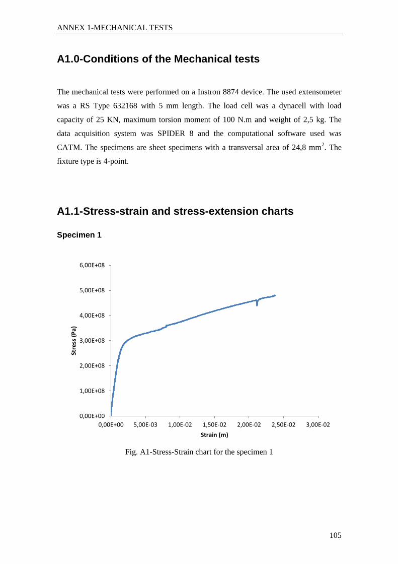
ANNEX 1-MECHANICAL TESTS
105
A1.0-Conditions of the Mechanical tests
The mechanical tests were performed on a Instron 8874 device. The used extensometer
was a RS Type 632168 with 5 mm length. The load cell was a dynacell with load
capacity of 25 KN, maximum torsion moment of 100 N.m and weight of 2,5 kg. The
data acquisition system was SPIDER 8 and the computational software used was
CATM. The specimens are sheet specimens with a transversal area of 24,8 mm2. The
fixture type is 4-point.
A1.1-Stress-strain and stress-extension charts
Specimen 1
Fig. A1-Stress-Strain chart for the specimen 1
0,00E+00
1,00E+08
2,00E+08
3,00E+08
4,00E+08
5,00E+08
6,00E+08
0,00E+00 5,00E-03 1,00E-02 1,50E-02 2,00E-02 2,50E-02 3,00E-02
Stre
ss (
Pa)
Strain (m)

ANNEX 1-MECHANICAL TESTS
106
Fig. A2-Stress-Extension chart for the specimen 1
Specimen 2
Fig. A3-Stress-Strain chart for the specimen 2
0,00E+00
1,00E+08
2,00E+08
3,00E+08
4,00E+08
5,00E+08
6,00E+08
7,00E+08
0,00 5,00 10,00 15,00 20,00 25,00 30,00 35,00
Stre
ss (
Pa)
Extension (mm)
0,00E+00
1,00E+08
2,00E+08
3,00E+08
4,00E+08
5,00E+08
6,00E+08
7,00E+08
8,00E+08
9,00E+08
0,00E+00 1,00E-02 2,00E-02 3,00E-02 4,00E-02 5,00E-02 6,00E-02
Stre
ss (
Pa)
Strain
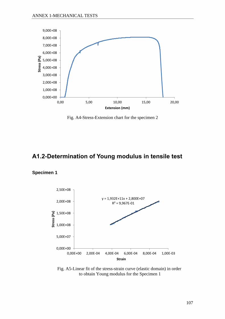
ANNEX 1-MECHANICAL TESTS
107
Fig. A4-Stress-Extension chart for the specimen 2
A1.2-Determination of Young modulus in tensile test
Specimen 1
Fig. A5-Linear fit of the stress-strain curve (elastic domain) in order
to obtain Young modulus for the Specimen 1
0,00E+00
1,00E+08
2,00E+08
3,00E+08
4,00E+08
5,00E+08
6,00E+08
7,00E+08
8,00E+08
9,00E+08
0,00 5,00 10,00 15,00 20,00
Stre
ss (
Pa)
Extension (mm)
y = 1,932E+11x + 2,800E+07 R² = 9,967E-01
0,00E+00
5,00E+07
1,00E+08
1,50E+08
2,00E+08
2,50E+08
0,00E+00 2,00E-04 4,00E-04 6,00E-04 8,00E-04 1,00E-03
Stre
ss (
Pa)
Strain

ANNEX 1-MECHANICAL TESTS
108
Specimen 2
Fig. A6-Linear fit of the stress-strain curve (elastic domain) in order
to obtain Young modulus for the Specimen 2
A1.3-Charts used to determine Yield stress
Specimen 1
Fig. A7-Determination of the Yield stress for the specimen 1
y = 1,682E+11x + 3,575E+07 R² = 9,960E-01
0,00E+00
5,00E+07
1,00E+08
1,50E+08
2,00E+08
2,50E+08
3,00E+08
3,50E+08
4,00E+08
4,50E+08
0,00E+00 5,00E-04 1,00E-03 1,50E-03 2,00E-03 2,50E-03
Stre
ss (
Pa)
Strain
0,00E+00
1,00E+08
2,00E+08
3,00E+08
4,00E+08
5,00E+08
6,00E+08
0,00E+00 5,00E-03 1,00E-02 1,50E-02 2,00E-02 2,50E-02 3,00E-02
Stre
ss (
Pa)
Strain

ANNEX 1-MECHANICAL TESTS
109
Specimen 2
Fig. A8-Determination of the Yield stress for the specimen 2
A1.4-Determination of Poisson coefficient and Young modulus in extensometry test
Load long transPoisson
coeficient Stress
Young
modulus(Pa)
Young
modulus(GPa)
2066 424 -124 0,2925 8,33E+07 1,9648E+11 196,48
3043 624 -126 0,2011 1,23E+08 1,9664E+11 196,64
4028 834 -248 0,2974 1,62E+08 1,9475E+11 194,75
5000 1103 -335 0,3037 2,02E+08 1,8279E+11 182,79
Table A1-Poisson coefficient, Normal Stress, and Young modulus for specimen 4,
1st read
Load long transPoisson
coeficient Stress
Young
modulus(Pa)
Young
modulus (GPa)
2010 416 -123 0,2957 8,10E+07 1,9483E+11 194,83
3100 634 -187 0,2950 1,25E+08 1,9716E+11 197,16
4040 821 -243 0,2960 1,63E+08 1,9842E+11 198,42
5010 1044 -311 0,2979 2,02E+08 1,9350E+11 193,50
Table A2-Poisson coefficient, Normal Stress, and Young modulus for specimen 4,
2nd
read
Load long trans Poisson
coeficient Stress
Young
modulus(Pa)
Young
modulus (GPa)
2060 459 -129 0,2810 8,31E+07 1,8097E+11 180,97
3010 663 -187 0,2821 1,21E+08 1,8306E+11 183,06
4060 885 -252 0,2847 1,64E+08 1,8498E+11 184,98
5020 1148 -333 0,2901 2,02E+08 1,7632E+11 176,32
Table A3-Poisson coefficient, Normal Stress, and Young modulus for specimen 5,
1st read
0,00E+00
1,00E+08
2,00E+08
3,00E+08
4,00E+08
5,00E+08
6,00E+08
7,00E+08
8,00E+08
9,00E+08
0,00E+00 1,00E-02 2,00E-02 3,00E-02 4,00E-02 5,00E-02 6,00E-02
Stre
ss (
Pa)
Strain

ANNEX 1-MECHANICAL TESTS
110
Load long trans Poisson
coeficient Stress
Young
modulus(Pa)
Young
modulus (GPa)
2100 465 -131 0,2817 8,5E+07 1,8210E+11 182,10
3100 676 -191 0,2825 1,3E+08 1,8491E+11 184,91
4045 873 -247 0,2829 1,6E+08 1,8683E+11 186,83
5050 1107 -315 0,2846 2E+08 1,8395E+11 183,95
Table A4-Poisson coefficient, Normal Stress, and Young modulus for specimen 5,
2nd
read
Load long trans Poisson
coeficient Stress
Young
modulus(Pa)
Young
modulus (GPa)
2018 437 -126 0,2883 8,14E+07 1,8620E+11 186,20
4030 859 -244 0,2841 1,63E+08 1,8917E+11 189,17
6020 1285 -369 0,2872 2,43E+08 1,8890E+11 188,90
Table A5-Poisson coefficient, Normal Stress, and Young modulus for specimen 6,
1st read
Load long trans Poisson
coeficient Stress
Young
modulus(Pa)
Young
modulus (GPa)
2040 428 -126 0,2944 8,23E+07 1,9219E+11 192,19
4050 852 -243 0,2852 1,63E+08 1,9167E+11 191,67
6100 1277 -365 0,2858 2,46E+08 1,9261E+11 192,61
Table A6-Poisson coefficient, Normal Stress, and Young modulus for specimen 6,
2nd
read
Load long trans Poisson
coeficient Stress
Young
modulus(Pa)
Young
modulus (GPa)
2120 420 -117 0,2786 8,55E+07 2,0353E+11 203,53
4060 867 -234 0,2699 1,64E+08 1,8882E+11 188,82
6060 1325 -355 0,2679 2,44E+08 1,8442E+11 184,42
Table A7-Poisson coefficient, Normal Stress, and Young modulus for specimen 7,
1st read
Load long transPoisson
coeficient Stress
Young
modulus(Pa)
Young
modulus (GPa)
2140 435 -118 0,2713 8,63E+07 1,9837E+11 198,37
4120 879 -235 0,2673 1,66E+08 1,8900E+11 189,00
6100 1313 -351 0,2673 2,46E+08 1,8733E+11 187,33
Table A8-Poisson coefficient, Normal Stress, and Young modulus for specimen 7,
2nd
read
111
ANNEX 2-VARIABLE ANALYSIS DATA

112

ANNEX 2-VARIABLE ANALYSIS
113
A2.1 Variable analysis data
A2.1.1 Model 1- Ribbed plate
A2.1.1.1 LG1 Variable
Variable
values LG1 0,01 0,015 0,02 0,025 0,03 0,035 0,04
LG2 0,051 0,051 0,051 0,051 0,051 0,051 0,051
LG3 0,0046 0,0046 0,0046 0,0046 0,0046 0,0046 0,0046
EX 2,10E+11 2,10E+11 2,10E+11 2,10E+11 2,10E+11 2,10E+11 2,10E+11
PXY 0,29 0,29 0,29 0,29 0,29 0,29 0,29
DNS 7890 7890 7890 7890 7890 7890 7890
Nodal
deflections Node 1 6,00E-07 1,10E-07 4,10E-07 9,50E-07 1,50E-06 2,10E-06 2,73E-06
Node 2 9,24E-06 8,26E-06 7,34E-06 6,49E-06 4,45E-06 3,88E-06 3,36E-06
Node 3 5,16E-05 4,88E-05 4,61E-05 4,34E-05 4,78E-05 4,53E-05 4,28E-05
Node 4 8,06E-06 7,20E-06 6,41E-06 5,66E-06 7,39E-05 6,94E-05 6,49E-05
Node 5 7,97E-05 7,58E-05 7,19E-05 6,80E-05 4,11E-05 3,81E-05 3,53E-05
Node 6 2,97E-05 2,77E-05 2,57E-05 2,38E-05 3,00E-04 2,95E-04 2,90E-04
Node 7 1,70E-05 1,58E-05 1,46E-05 1,35E-05 4,60E-04 4,53E-04 4,47E-04
Node 8 5,19E-06 4,82E-06 4,48E-06 4,15E-06 1,06E-03 1,05E-03 1,04E-03
Node 9 4,83E-04 4,77E-04 4,71E-04 4,66E-04 3,34E-04 3,30E-04 3,24E-04
Node 10 1,32E-04 1,30E-04 1,27E-04 1,24E-04 1,05E-04 1,02E-04 1,00E-04
Node 11 2,42E-05 2,39E-05 2,34E-05 2,30E-05 9,44E-05 9,24E-05 9,02E-05
Node 12 8,53E-06 8,39E-06 8,25E-06 8,08E-06 5,34E-05 5,66E-05 6,01E-05
Node 13 8,72E-05 8,60E-05 8,46E-05 8,31E-05 3,90E-05 4,13E-05 4,38E-05
Node 14 1,12E-05 1,18E-05 1,24E-05 1,31E-05 5,33E-05 5,65E-05 6,00E-05
Node 15 3,99E-05 4,22E-05 4,46E-05 4,71E-05 8,09E-05 7,92E-05 7,72E-05
Objective
function q(x) 9,87E-04 9,67E-04 9,48E-04 9,30E-04 2,75E-03 2,71E-03 2,68E-03
Table A9-Variable values, obtained nodal deflections, and objective function for the
LG1 variable analysis (ribbed plate model)

ANNEX 2-VARIABLE ANALYSIS
114
A2.1.1.2 LG2 Variable
Variable
values LG1 0,025 0,025 0,025 0,025 0,025 0,025 0,025
LG2 0,035 0,04 0,045 0,05 0,055 0,06 0,065
LG3 0,0046 0,0046 0,0046 0,0046 0,0046 0,0046 0,0046
EX 2,10E+11 2,10E+11 2,10E+11 2,10E+11 2,10E+11 2,10E+11 2,10E+11
PXY 0,29 0,29 0,29 0,29 0,29 0,29 0,29
DNS 7890 7890 7890 7890 7890 7890 7890
Nodal
deflections Node 1 2,56E-06 1,20E-06 1,10E-06 9,50E-07 7,90E-07 6,70E-07 9,00E-08
Node 2 9,12E-05 6,62E-06 6,56E-06 6,49E-06 6,43E-06 6,38E-06 6,00E-08
Node 3 7,68E-05 4,85E-05 4,56E-05 4,34E-05 4,18E-05 4,07E-05 1,12E-06
Node 4 4,42E-05 5,81E-06 5,73E-06 5,66E-06 5,60E-06 5,55E-06 6,15E-05
Node 5 8,30E-06 7,64E-05 7,15E-05 6,80E-05 6,54E-05 6,37E-05 7,01E-05
Node 6 3,77E-04 2,59E-05 2,47E-05 2,38E-05 2,32E-05 2,27E-05 5,52E-05
Node 7 4,89E-04 1,44E-05 1,39E-05 1,35E-05 1,32E-05 1,29E-05 7,57E-05
Node 8 9,31E-05 4,69E-06 4,38E-06 4,15E-06 3,98E-06 3,88E-06 6,71E-05
Node 9 8,74E-05 4,80E-04 4,72E-04 4,66E-04 4,61E-04 4,57E-04 2,59E-05
Node 10 4,91E-04 1,28E-04 1,26E-04 1,24E-04 1,22E-04 1,21E-04 2,62E-05
Node 11 1,13E-04 3,81E-05 2,91E-05 2,30E-05 1,87E-05 1,60E-05 5,95E-05
Node 12 3,03E-05 1,31E-05 1,01E-05 8,08E-06 6,66E-06 5,80E-06 9,78E-04
Node 13 1,67E-04 1,40E-04 1,06E-04 8,31E-05 6,67E-05 5,68E-05 1,50E-04
Node 14 3,17E-06 2,20E-05 1,67E-05 1,31E-05 1,06E-05 9,03E-06 1,42E-05
Node 15 5,13E-06 8,12E-05 6,09E-05 4,71E-05 3,75E-05 3,18E-05 5,25E-05
Objective
function q(x) 2,08E-03 1,09E-03 9,94E-04 9,30E-04 8,83E-04 8,55E-04 1,64E-03
Table A10-Variable values, obtained nodal deflections, and objective function for the
LG2 variable analysis (ribbed plate model)

ANNEX 2-VARIABLE ANALYSIS
115
A2.1.1.3 LG3 Variable
Variable
values LG1 0,025 0,025 0,025 0,025 0,025 0,025 0,025
LG2 0,051 0,051 0,051 0,051 0,051 0,051 0,051
LG3 0,0031 0,0036 0,0041 0,0046 0,0051 0,0056 0,0061
EX 2,10E+11 2,10E+11 2,10E+11 2,10E+11 2,10E+11 2,10E+11 2,10E+11
PXY 0,29 0,29 0,29 0,29 0,29 0,29 0,29
DNS 7890 7890 7890 7890 7890 7890 7890
Nodal
deflections Node 1 1,80E-06 1,45E-06 1,17E-06 9,50E-07 7,50E-07 5,90E-07 4,50E-07
Node 2 2,15E-05 1,37E-05 9,21E-06 6,49E-06 4,74E-06 3,56E-06 2,73E-06
Node 3 1,32E-04 8,60E-05 5,97E-05 4,34E-05 3,28E-05 2,56E-05 2,05E-05
Node 4 1,86E-05 1,19E-05 8,01E-06 5,66E-06 4,15E-06 3,13E-06 2,41E-06
Node 5 2,05E-04 1,34E-04 9,32E-05 6,80E-05 5,16E-05 4,04E-05 3,24E-05
Node 6 7,45E-05 4,82E-05 3,31E-05 2,38E-05 1,78E-05 1,37E-05 1,09E-05
Node 7 4,27E-05 2,75E-05 1,88E-05 1,35E-05 1,00E-05 7,69E-06 6,05E-06
Node 8 1,23E-05 8,10E-06 5,66E-06 4,15E-06 3,16E-06 2,49E-06 2,01E-06
Node 9 1,49E-03 9,59E-04 6,53E-04 4,66E-04 3,44E-04 2,62E-04 2,05E-04
Node 10 3,98E-04 2,56E-04 1,74E-04 1,24E-04 9,16E-05 6,98E-05 5,45E-05
Node 11 3,45E-05 2,96E-05 2,59E-05 2,30E-05 2,07E-05 1,87E-05 1,71E-05
Node 12 1,21E-05 1,04E-05 9,10E-06 8,08E-06 7,27E-06 6,59E-06 6,03E-06
Node 13 1,25E-04 1,07E-04 9,36E-05 8,31E-05 7,47E-05 6,77E-05 6,18E-05
Node 14 1,94E-05 1,67E-05 1,47E-05 1,31E-05 1,18E-05 1,08E-05 9,91E-06
Node 15 6,96E-05 6,01E-05 5,28E-05 4,71E-05 4,26E-05 3,89E-05 3,57E-05
Objective
function q(x) 2,66E-03 1,77E-03 1,25E-03 9,30E-04 7,18E-04 5,72E-04 4,67E-04
Table A11-Variable values, obtained nodal deflections, and objective function for the
LG3 variable analysis (ribbed plate model)
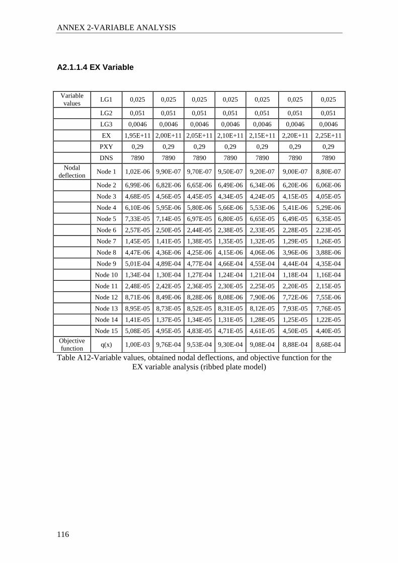
ANNEX 2-VARIABLE ANALYSIS
116
A2.1.1.4 EX Variable
Table A12-Variable values, obtained nodal deflections, and objective function for the
EX variable analysis (ribbed plate model)
Variable
values LG1 0,025 0,025 0,025 0,025 0,025 0,025 0,025
LG2 0,051 0,051 0,051 0,051 0,051 0,051 0,051
LG3 0,0046 0,0046 0,0046 0,0046 0,0046 0,0046 0,0046
EX 1,95E+11 2,00E+11 2,05E+11 2,10E+11 2,15E+11 2,20E+11 2,25E+11
PXY 0,29 0,29 0,29 0,29 0,29 0,29 0,29
DNS 7890 7890 7890 7890 7890 7890 7890
Nodal
deflection Node 1 1,02E-06 9,90E-07 9,70E-07 9,50E-07 9,20E-07 9,00E-07 8,80E-07
Node 2 6,99E-06 6,82E-06 6,65E-06 6,49E-06 6,34E-06 6,20E-06 6,06E-06
Node 3 4,68E-05 4,56E-05 4,45E-05 4,34E-05 4,24E-05 4,15E-05 4,05E-05
Node 4 6,10E-06 5,95E-06 5,80E-06 5,66E-06 5,53E-06 5,41E-06 5,29E-06
Node 5 7,33E-05 7,14E-05 6,97E-05 6,80E-05 6,65E-05 6,49E-05 6,35E-05
Node 6 2,57E-05 2,50E-05 2,44E-05 2,38E-05 2,33E-05 2,28E-05 2,23E-05
Node 7 1,45E-05 1,41E-05 1,38E-05 1,35E-05 1,32E-05 1,29E-05 1,26E-05
Node 8 4,47E-06 4,36E-06 4,25E-06 4,15E-06 4,06E-06 3,96E-06 3,88E-06
Node 9 5,01E-04 4,89E-04 4,77E-04 4,66E-04 4,55E-04 4,44E-04 4,35E-04
Node 10 1,34E-04 1,30E-04 1,27E-04 1,24E-04 1,21E-04 1,18E-04 1,16E-04
Node 11 2,48E-05 2,42E-05 2,36E-05 2,30E-05 2,25E-05 2,20E-05 2,15E-05
Node 12 8,71E-06 8,49E-06 8,28E-06 8,08E-06 7,90E-06 7,72E-06 7,55E-06
Node 13 8,95E-05 8,73E-05 8,52E-05 8,31E-05 8,12E-05 7,93E-05 7,76E-05
Node 14 1,41E-05 1,37E-05 1,34E-05 1,31E-05 1,28E-05 1,25E-05 1,22E-05
Node 15 5,08E-05 4,95E-05 4,83E-05 4,71E-05 4,61E-05 4,50E-05 4,40E-05
Objective
function q(x) 1,00E-03 9,76E-04 9,53E-04 9,30E-04 9,08E-04 8,88E-04 8,68E-04

ANNEX 2-VARIABLE ANALYSIS
117
A2.1.1.5 PXY Variable
Variable
values LG1 0,025 0,025 0,025 0,025 0,025 0,025 0,025
LG2 0,051 0,051 0,051 0,051 0,051 0,051 0,051
LG3 0,0046 0,0046 0,0046 0,0046 0,0046 0,0046 0,0046
EX 2,10E+11 2,10E+11 2,10E+11 2,10E+11 2,10E+11 2,10E+11 2,10E+11
PXY 0,23 0,25 0,27 0,29 0,31 0,33 0,35
DNS 7890 7890 7890 7890 7890 7890 7890
Nodal
deflection Node 1 7,20E-07 7,90E-07 8,70E-07 9,50E-07 1,02E-06 1,10E-06 1,18E-06
Node 2 6,76E-06 6,67E-06 6,58E-06 6,49E-06 6,39E-06 6,29E-06 6,18E-06
Node 3 4,46E-05 4,42E-05 4,39E-05 4,34E-05 4,30E-05 4,25E-05 4,20E-05
Node 4 5,91E-06 5,83E-06 5,75E-06 5,66E-06 5,57E-06 5,48E-06 5,38E-06
Node 5 6,97E-05 6,92E-05 6,87E-05 6,80E-05 6,74E-05 6,66E-05 6,59E-05
Node 6 2,46E-05 2,44E-05 2,41E-05 2,38E-05 2,35E-05 2,32E-05 2,29E-05
Node 7 1,40E-05 1,38E-05 1,37E-05 1,35E-05 1,33E-05 1,31E-05 1,29E-05
Node 8 4,29E-06 4,25E-06 4,20E-06 4,15E-06 4,10E-06 4,05E-06 3,99E-06
Node 9 4,81E-04 4,76E-04 4,71E-04 4,66E-04 4,60E-04 4,54E-04 4,47E-04
Node 10 1,29E-04 1,27E-04 1,26E-04 1,24E-04 1,22E-04 1,20E-04 1,18E-04
Node 11 2,31E-05 2,31E-05 2,30E-05 2,30E-05 2,30E-05 2,29E-05 2,29E-05
Node 12 8,18E-06 8,15E-06 8,12E-06 8,08E-06 8,05E-06 8,02E-06 7,99E-06
Node 13 8,35E-05 8,34E-05 8,33E-05 8,31E-05 8,30E-05 8,28E-05 8,27E-05
Node 14 1,31E-05 1,31E-05 1,31E-05 1,31E-05 1,31E-05 1,31E-05 1,31E-05
Node 15 4,71E-05 4,71E-05 4,71E-05 4,71E-05 4,72E-05 4,72E-05 4,72E-05
Objective
function q(x) 9,55E-04 9,47E-04 9,39E-04 9,30E-04 9,20E-04 9,10E-04 8,99E-04
Table A13-Variable values, obtained nodal deflections, and objective function for the
PXY variable analysis (ribbed plate model)
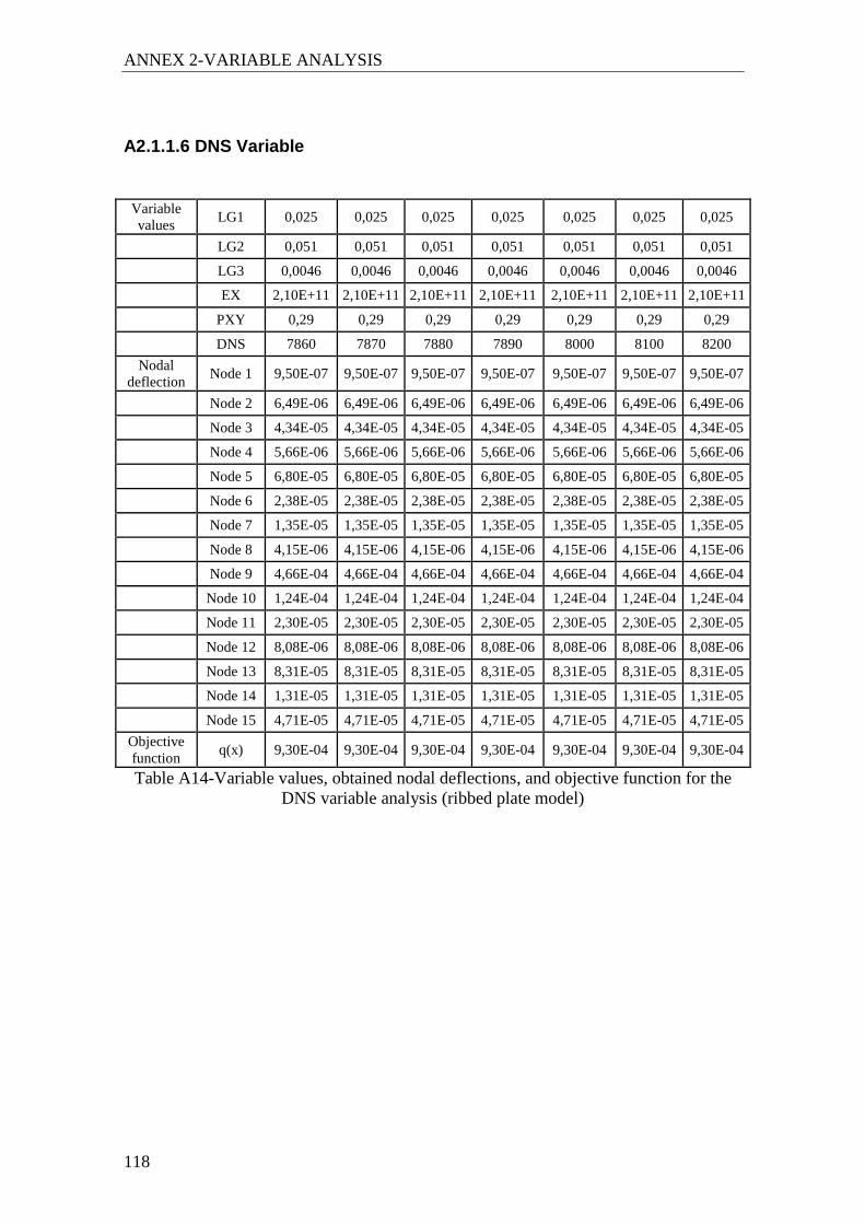
ANNEX 2-VARIABLE ANALYSIS
118
A2.1.1.6 DNS Variable
Table A14-Variable values, obtained nodal deflections, and objective function for the
DNS variable analysis (ribbed plate model)
Variable
values LG1 0,025 0,025 0,025 0,025 0,025 0,025 0,025
LG2 0,051 0,051 0,051 0,051 0,051 0,051 0,051
LG3 0,0046 0,0046 0,0046 0,0046 0,0046 0,0046 0,0046
EX 2,10E+11 2,10E+11 2,10E+11 2,10E+11 2,10E+11 2,10E+11 2,10E+11
PXY 0,29 0,29 0,29 0,29 0,29 0,29 0,29
DNS 7860 7870 7880 7890 8000 8100 8200
Nodal
deflection Node 1 9,50E-07 9,50E-07 9,50E-07 9,50E-07 9,50E-07 9,50E-07 9,50E-07
Node 2 6,49E-06 6,49E-06 6,49E-06 6,49E-06 6,49E-06 6,49E-06 6,49E-06
Node 3 4,34E-05 4,34E-05 4,34E-05 4,34E-05 4,34E-05 4,34E-05 4,34E-05
Node 4 5,66E-06 5,66E-06 5,66E-06 5,66E-06 5,66E-06 5,66E-06 5,66E-06
Node 5 6,80E-05 6,80E-05 6,80E-05 6,80E-05 6,80E-05 6,80E-05 6,80E-05
Node 6 2,38E-05 2,38E-05 2,38E-05 2,38E-05 2,38E-05 2,38E-05 2,38E-05
Node 7 1,35E-05 1,35E-05 1,35E-05 1,35E-05 1,35E-05 1,35E-05 1,35E-05
Node 8 4,15E-06 4,15E-06 4,15E-06 4,15E-06 4,15E-06 4,15E-06 4,15E-06
Node 9 4,66E-04 4,66E-04 4,66E-04 4,66E-04 4,66E-04 4,66E-04 4,66E-04
Node 10 1,24E-04 1,24E-04 1,24E-04 1,24E-04 1,24E-04 1,24E-04 1,24E-04
Node 11 2,30E-05 2,30E-05 2,30E-05 2,30E-05 2,30E-05 2,30E-05 2,30E-05
Node 12 8,08E-06 8,08E-06 8,08E-06 8,08E-06 8,08E-06 8,08E-06 8,08E-06
Node 13 8,31E-05 8,31E-05 8,31E-05 8,31E-05 8,31E-05 8,31E-05 8,31E-05
Node 14 1,31E-05 1,31E-05 1,31E-05 1,31E-05 1,31E-05 1,31E-05 1,31E-05
Node 15 4,71E-05 4,71E-05 4,71E-05 4,71E-05 4,71E-05 4,71E-05 4,71E-05
Objective
function q(x) 9,30E-04 9,30E-04 9,30E-04 9,30E-04 9,30E-04 9,30E-04 9,30E-04

ANNEX 2-VARIABLE ANALYSIS
119
A2.1.2 Model 2- Tubular beam
A2.1.2.1 LG4 Variable
Table A15-Variable values, obtained nodal deflections, and objective function for the
LG4 variable analysis (tubular beam model)
Variable
values LG4 0,015 0,017 0,019 0,021 0,023 0,025 0,027
LG5 0,008 0,008 0,008 0,008 0,008 0,008 0,008
LG6 0,081 0,081 0,081 0,081 0,081 0,081 0,081
EX 2,10E+11 2,10E+11 2,10E+11 2,10E+11 2,10E+11 2,10E+11 2,10E+11
PXY 0,29 0,29 0,29 0,29 0,29 0,29 0,29
DNS 7890 7890 7890 7890 7890 7890 7890
Nodal
deflection Node 1 2,60E-07 3,50E-07 5,30E-07 7,90E-07 1,14E-06 1,57E-06 2,09E-06
Node 2 5,00E-08 5,00E-08 5,00E-08 5,00E-08 4,00E-08 4,00E-08 4,00E-08
Node 3 1,08E-06 1,00E-06 8,70E-07 7,00E-07 5,00E-07 2,60E-07 2,00E-08
Node 4 2,66E-06 2,72E-06 2,68E-06 2,57E-06 2,39E-06 2,13E-06 1,81E-06
Node 5 1,05E-05 1,13E-05 1,21E-05 1,30E-05 1,39E-05 1,49E-05 1,60E-05
Node 6 2,00E-08 1,00E-08 0,00E+00 1,00E-08 2,00E-08 3,00E-08 3,00E-08
Node 7 4,09E-06 4,45E-06 4,82E-06 5,22E-06 5,63E-06 6,07E-06 6,54E-06
Node 8 9,53E-06 1,03E-05 1,10E-05 1,19E-05 1,27E-05 1,36E-05 1,46E-05
Node 9 1,92E-04 2,00E-04 2,06E-04 2,11E-04 2,15E-04 2,18E-04 2,20E-04
Node 10 3,90E-06 4,23E-06 4,54E-06 4,85E-06 5,16E-06 5,48E-06 5,80E-06
Node 11 6,49E-05 6,69E-05 6,84E-05 6,96E-05 7,04E-05 7,10E-05 7,14E-05
Node 12 1,78E-04 1,85E-04 1,92E-04 1,97E-04 2,01E-04 2,04E-04 2,06E-04
Node 13 1,00E-08 1,00E-08 1,00E-08 1,00E-08 1,00E-08 1,00E-08 1,00E-08
Node 14 1,20E-07 1,30E-07 1,50E-07 1,70E-07 1,90E-07 2,20E-07 2,50E-07
Node 15 3,00E-08 3,00E-08 4,00E-08 5,00E-08 7,00E-08 8,00E-08 9,00E-08
Node 16 0,00E+00 0,00E+00 0,00E+00 0,00E+00 0,00E+00 0,00E+00 0,00E+00
Node 17 6,00E-08 6,00E-08 6,00E-08 6,00E-08 6,00E-08 5,00E-08 5,00E-08
Node 18 2,00E-08 2,00E-08 2,00E-08 2,00E-08 1,00E-08 1,00E-08 1,00E-08
Node 19 0,00E+00 0,00E+00 0,00E+00 0,00E+00 0,00E+00 0,00E+00 0,00E+00
Node 20 1,00E-07 1,00E-07 1,00E-07 9,00E-08 9,00E-08 9,00E-08 8,00E-08
Node 21 4,00E-08 4,00E-08 3,00E-08 3,00E-08 3,00E-08 3,00E-08 3,00E-08
Objective
function q(x) 4,67E-04 4,87E-04 5,03E-04 5,17E-04 5,28E-04 5,37E-04 5,45E-04

ANNEX 2-VARIABLE ANALYSIS
120
A2.1.2.2 LG5 Variable
Variable
values LG4 0,021 0,021 0,021 0,021 0,021 0,021 0,021
LG5 0,005 0,006 0,007 0,008 0,009 0,01 0,011
LG6 0,081 0,081 0,081 0,081 0,081 0,081 0,081
EX 2,10E+11 2,10E+11 2,10E+11 2,10E+11 2,10E+11 2,10E+11 2,10E+11
PXY 0,29 0,29 0,29 0,29 0,29 0,29 0,29
DNS 7890 7890 7890 7890 7890 7890 7890
Nodal
deflections Node 1 5,09E-06 3,22E-06 1,25E-06 7,90E-07 2,86E-06 4,92E-06 1,12E-05
Node 2 8,00E-08 6,00E-08 5,00E-08 5,00E-08 6,00E-08 7,00E-08 1,25E-05
Node 3 2,61E-06 1,92E-06 1,30E-06 7,00E-07 9,00E-08 5,80E-07 3,10E-06
Node 4 7,12E-06 5,73E-06 4,21E-06 2,57E-06 8,60E-07 8,80E-07 6,52E-06
Node 5 6,25E-06 8,53E-06 1,08E-05 1,30E-05 1,52E-05 1,72E-05 1,81E-05
Node 6 6,00E-08 4,00E-08 2,00E-08 1,00E-08 0,00E+00 1,00E-08 1,91E-05
Node 7 3,10E-06 3,79E-06 4,50E-06 5,22E-06 5,94E-06 6,65E-06 5,28E-06
Node 8 5,76E-06 7,79E-06 9,84E-06 1,19E-05 1,38E-05 1,57E-05 1,58E-05
Node 9 2,23E-04 2,20E-04 2,16E-04 2,11E-04 2,05E-04 1,97E-04 1,35E-04
Node 10 8,87E-06 6,71E-06 5,27E-06 4,85E-06 5,33E-06 6,39E-06 2,38E-06
Node 11 6,96E-05 6,73E-05 6,75E-05 6,96E-05 7,25E-05 7,55E-05 6,12E-05
Node 12 1,95E-04 1,97E-04 1,98E-04 1,97E-04 1,95E-04 1,92E-04 1,62E-04
Node 13 2,00E-08 1,00E-08 1,00E-08 1,00E-08 1,00E-08 1,00E-08 1,00E-08
Node 14 9,00E-08 0,00E+00 9,00E-08 1,70E-07 2,40E-07 3,10E-07 2,00E-08
Node 15 4,00E-08 0,00E+00 3,00E-08 5,00E-08 8,00E-08 1,00E-07 0,00E+00
Node 16 0,00E+00 0,00E+00 0,00E+00 0,00E+00 0,00E+00 0,00E+00 3,00E-08
Node 17 1,00E-07 9,00E-08 7,00E-08 6,00E-08 5,00E-08 3,00E-08 3,50E-07
Node 18 3,00E-08 3,00E-08 2,00E-08 2,00E-08 1,00E-08 1,00E-08 1,30E-07
Node 19 0,00E+00 0,00E+00 0,00E+00 0,00E+00 0,00E+00 0,00E+00 0,00E+00
Node 20 1,00E-07 1,00E-07 1,00E-07 9,00E-08 9,00E-08 9,00E-08 8,00E-08
Node 21 4,00E-08 4,00E-08 3,00E-08 3,00E-08 3,00E-08 3,00E-08 4,00E-08
Objective
function q(x) 5,27E-04 5,23E-04 5,19E-04 5,17E-04 5,16E-04 5,17E-04 4,53E-04
Table A16-Variable values, obtained nodal deflections, and objective function for the
LG5 variable analysis (tubular beam model)

ANNEX 2-VARIABLE ANALYSIS
121
A2.1.2.3 LG6 Variable
Table A17-Variable values, obtained nodal deflections, and objective function for the
LG6 variable analysis (tubular beam model)
Variable
values LG4 0,021 0,021 0,021 0,021 0,021 0,021 0,021
LG5 0,008 0,008 0,008 0,008 0,008 0,008 0,008
LG6 0,066 0,071 0,076 0,081 0,086 0,091 0,096
EX 2,10E+11 2,10E+11 2,10E+11 2,10E+11 2,10E+11 2,10E+11 2,10E+11
PXY 0,29 0,29 0,29 0,29 0,29 0,29 0,29
DNS 7890 7890 7890 7890 7890 7890 7890
Nodal
deflections Node 1 0,00E+00 0,00E+00 0,00E+00 7,90E-07 6,30E-07 4,80E-07 3,60E-07
Node 2 4,60E-07 4,20E-07 3,90E-07 5,00E-08 5,00E-08 7,00E-08 8,00E-08
Node 3 3,60E-07 3,40E-07 3,40E-07 7,00E-07 8,10E-07 9,20E-07 1,03E-06
Node 4 6,85E-06 6,43E-06 6,12E-06 2,57E-06 2,55E-06 2,53E-06 2,51E-06
Node 5 1,60E-04 1,34E-04 1,12E-04 1,30E-05 1,27E-05 1,24E-05 1,22E-05
Node 6 1,89E-04 1,57E-04 1,31E-04 1,00E-08 2,00E-08 2,00E-08 3,00E-08
Node 7 2,32E-04 1,87E-04 1,50E-04 5,22E-06 5,05E-06 4,91E-06 4,81E-06
Node 8 8,92E-05 7,56E-05 6,51E-05 1,19E-05 1,15E-05 1,13E-05 1,11E-05
Node 9 1,04E-06 1,02E-06 9,30E-07 2,11E-04 1,96E-04 1,83E-04 1,72E-04
Node 10 1,65E-05 1,43E-05 1,29E-05 4,85E-06 4,66E-06 4,79E-06 5,16E-06
Node 11 8,22E-05 7,66E-05 7,26E-05 6,96E-05 6,62E-05 6,39E-05 6,24E-05
Node 12 4,00E-07 4,00E-07 3,60E-07 1,97E-04 1,85E-04 1,76E-04 1,68E-04
Node 13 1,60E-07 1,40E-07 1,20E-07 1,00E-08 1,00E-08 1,00E-08 1,00E-08
Node 14 7,00E-08 6,00E-08 5,00E-08 1,70E-07 1,60E-07 1,60E-07 1,60E-07
Node 15 0,00E+00 0,00E+00 0,00E+00 5,00E-08 5,00E-08 4,00E-08 4,00E-08
Node 16 6,10E-07 4,50E-07 3,30E-07 0,00E+00 0,00E+00 0,00E+00 0,00E+00
Node 17 3,60E-07 2,80E-07 2,30E-07 6,00E-08 5,00E-08 5,00E-08 4,00E-08
Node 18 6,00E-08 5,00E-08 4,00E-08 2,00E-08 1,00E-08 1,00E-08 1,00E-08
Node 19 1,02E-05 9,23E-06 8,46E-06 0,00E+00 0,00E+00 0,00E+00 0,00E+00
Node 20 4,05E-06 3,52E-06 3,07E-06 9,00E-08 8,00E-08 6,00E-08 5,00E-08
Node 21 1,57E-05 1,41E-05 1,28E-05 3,00E-08 3,00E-08 2,00E-08 2,00E-08
Objective
function q(x) 8,10E-04 6,80E-04 5,78E-04 5,17E-04 4,86E-04 4,61E-04 4,40E-04
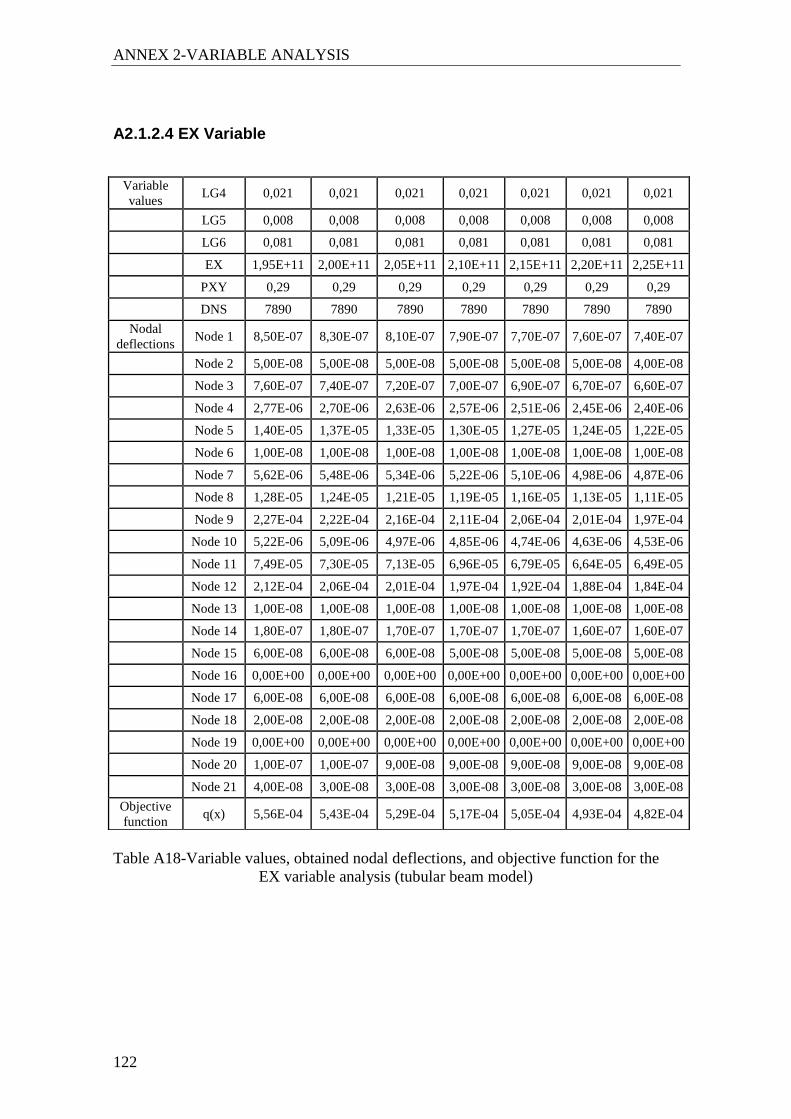
ANNEX 2-VARIABLE ANALYSIS
122
A2.1.2.4 EX Variable
Table A18-Variable values, obtained nodal deflections, and objective function for the
EX variable analysis (tubular beam model)
Variable
values LG4 0,021 0,021 0,021 0,021 0,021 0,021 0,021
LG5 0,008 0,008 0,008 0,008 0,008 0,008 0,008
LG6 0,081 0,081 0,081 0,081 0,081 0,081 0,081
EX 1,95E+11 2,00E+11 2,05E+11 2,10E+11 2,15E+11 2,20E+11 2,25E+11
PXY 0,29 0,29 0,29 0,29 0,29 0,29 0,29
DNS 7890 7890 7890 7890 7890 7890 7890
Nodal
deflections Node 1 8,50E-07 8,30E-07 8,10E-07 7,90E-07 7,70E-07 7,60E-07 7,40E-07
Node 2 5,00E-08 5,00E-08 5,00E-08 5,00E-08 5,00E-08 5,00E-08 4,00E-08
Node 3 7,60E-07 7,40E-07 7,20E-07 7,00E-07 6,90E-07 6,70E-07 6,60E-07
Node 4 2,77E-06 2,70E-06 2,63E-06 2,57E-06 2,51E-06 2,45E-06 2,40E-06
Node 5 1,40E-05 1,37E-05 1,33E-05 1,30E-05 1,27E-05 1,24E-05 1,22E-05
Node 6 1,00E-08 1,00E-08 1,00E-08 1,00E-08 1,00E-08 1,00E-08 1,00E-08
Node 7 5,62E-06 5,48E-06 5,34E-06 5,22E-06 5,10E-06 4,98E-06 4,87E-06
Node 8 1,28E-05 1,24E-05 1,21E-05 1,19E-05 1,16E-05 1,13E-05 1,11E-05
Node 9 2,27E-04 2,22E-04 2,16E-04 2,11E-04 2,06E-04 2,01E-04 1,97E-04
Node 10 5,22E-06 5,09E-06 4,97E-06 4,85E-06 4,74E-06 4,63E-06 4,53E-06
Node 11 7,49E-05 7,30E-05 7,13E-05 6,96E-05 6,79E-05 6,64E-05 6,49E-05
Node 12 2,12E-04 2,06E-04 2,01E-04 1,97E-04 1,92E-04 1,88E-04 1,84E-04
Node 13 1,00E-08 1,00E-08 1,00E-08 1,00E-08 1,00E-08 1,00E-08 1,00E-08
Node 14 1,80E-07 1,80E-07 1,70E-07 1,70E-07 1,70E-07 1,60E-07 1,60E-07
Node 15 6,00E-08 6,00E-08 6,00E-08 5,00E-08 5,00E-08 5,00E-08 5,00E-08
Node 16 0,00E+00 0,00E+00 0,00E+00 0,00E+00 0,00E+00 0,00E+00 0,00E+00
Node 17 6,00E-08 6,00E-08 6,00E-08 6,00E-08 6,00E-08 6,00E-08 6,00E-08
Node 18 2,00E-08 2,00E-08 2,00E-08 2,00E-08 2,00E-08 2,00E-08 2,00E-08
Node 19 0,00E+00 0,00E+00 0,00E+00 0,00E+00 0,00E+00 0,00E+00 0,00E+00
Node 20 1,00E-07 1,00E-07 9,00E-08 9,00E-08 9,00E-08 9,00E-08 9,00E-08
Node 21 4,00E-08 3,00E-08 3,00E-08 3,00E-08 3,00E-08 3,00E-08 3,00E-08
Objective
function q(x) 5,56E-04 5,43E-04 5,29E-04 5,17E-04 5,05E-04 4,93E-04 4,82E-04

ANNEX 2-VARIABLE ANALYSIS
123
A2.1.2.5 PXY Variable
Table A19-Variable values, obtained nodal deflections, and objective function for the
PXY variable analysis (tubular beam model)
Variable
values LG4 0,021 0,021 0,021 0,021 0,021 0,021 0,021
LG5 0,008 0,008 0,008 0,008 0,008 0,008 0,008
LG6 0,081 0,081 0,081 0,081 0,081 0,081 0,081
EX 2,10E+11 2,10E+11 2,10E+11 2,10E+11 2,10E+11 2,10E+11 2,10E+11
PXY 0,23 0,25 0,27 0,29 0,31 0,33 0,35
DNS 7890 7890 7890 7890 7890 7890 7890
Nodal
deflections Node 1 6,90E-07 7,20E-07 7,60E-07 7,90E-07 8,30E-07 8,70E-07 9,10E-07
Node 2 5,00E-08 5,00E-08 5,00E-08 5,00E-08 5,00E-08 5,00E-08 5,00E-08
Node 3 7,50E-07 7,40E-07 7,20E-07 7,00E-07 6,90E-07 6,70E-07 6,50E-07
Node 4 2,66E-06 2,64E-06 2,60E-06 2,57E-06 2,54E-06 2,50E-06 2,46E-06
Node 5 1,31E-05 1,31E-05 1,30E-05 1,30E-05 1,30E-05 1,30E-05 1,30E-05
Node 6 2,00E-08 2,00E-08 1,00E-08 1,00E-08 0,00E+00 0,00E+00 1,00E-08
Node 7 5,24E-06 5,24E-06 5,23E-06 5,22E-06 5,21E-06 5,20E-06 5,19E-06
Node 8 1,19E-05 1,19E-05 1,19E-05 1,19E-05 1,18E-05 1,18E-05 1,18E-05
Node 9 2,15E-04 2,14E-04 2,12E-04 2,11E-04 2,10E-04 2,08E-04 2,07E-04
Node 10 4,93E-06 4,91E-06 4,88E-06 4,85E-06 4,82E-06 4,80E-06 4,77E-06
Node 11 7,07E-05 7,03E-05 7,00E-05 6,96E-05 6,91E-05 6,87E-05 6,82E-05
Node 12 2,01E-04 1,99E-04 1,98E-04 1,97E-04 1,95E-04 1,93E-04 1,92E-04
Node 13 1,00E-08 1,00E-08 1,00E-08 1,00E-08 1,00E-08 1,00E-08 1,00E-08
Node 14 1,70E-07 1,70E-07 1,70E-07 1,70E-07 1,70E-07 1,70E-07 1,70E-07
Node 15 5,00E-08 5,00E-08 5,00E-08 5,00E-08 5,00E-08 6,00E-08 6,00E-08
Node 16 0,00E+00 0,00E+00 0,00E+00 0,00E+00 0,00E+00 0,00E+00 0,00E+00
Node 17 6,00E-08 6,00E-08 6,00E-08 6,00E-08 6,00E-08 6,00E-08 6,00E-08
Node 18 2,00E-08 2,00E-08 2,00E-08 2,00E-08 2,00E-08 2,00E-08 2,00E-08
Node 19 0,00E+00 0,00E+00 0,00E+00 0,00E+00 0,00E+00 0,00E+00 0,00E+00
Node 20 9,00E-08 9,00E-08 9,00E-08 9,00E-08 9,00E-08 9,00E-08 9,00E-08
Node 21 3,00E-08 3,00E-08 3,00E-08 3,00E-08 3,00E-08 3,00E-08 3,00E-08
Objective
function q(x) 5,26E-04 5,23E-04 5,20E-04 5,17E-04 5,13E-04 5,10E-04 5,06E-04
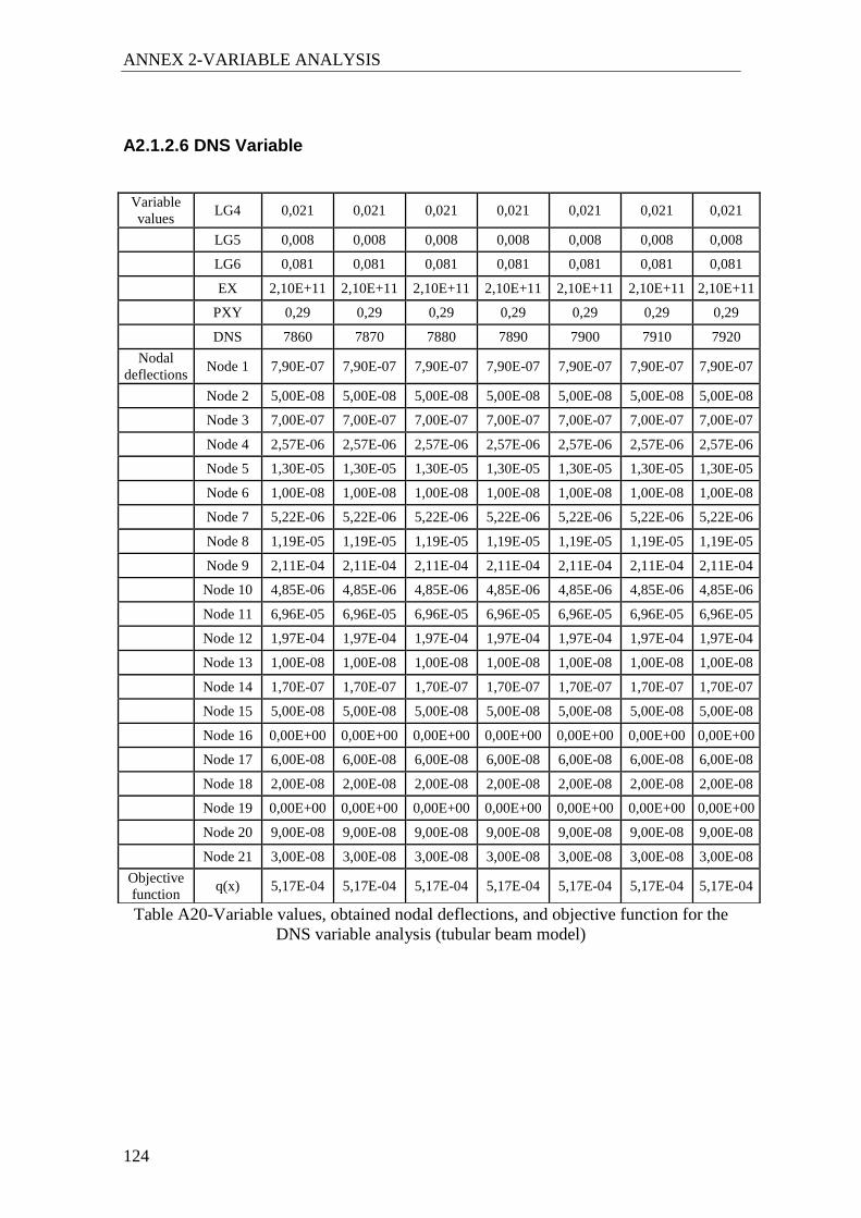
ANNEX 2-VARIABLE ANALYSIS
124
A2.1.2.6 DNS Variable
Table A20-Variable values, obtained nodal deflections, and objective function for the
DNS variable analysis (tubular beam model)
Variable
values LG4 0,021 0,021 0,021 0,021 0,021 0,021 0,021
LG5 0,008 0,008 0,008 0,008 0,008 0,008 0,008
LG6 0,081 0,081 0,081 0,081 0,081 0,081 0,081
EX 2,10E+11 2,10E+11 2,10E+11 2,10E+11 2,10E+11 2,10E+11 2,10E+11
PXY 0,29 0,29 0,29 0,29 0,29 0,29 0,29
DNS 7860 7870 7880 7890 7900 7910 7920
Nodal
deflections Node 1 7,90E-07 7,90E-07 7,90E-07 7,90E-07 7,90E-07 7,90E-07 7,90E-07
Node 2 5,00E-08 5,00E-08 5,00E-08 5,00E-08 5,00E-08 5,00E-08 5,00E-08
Node 3 7,00E-07 7,00E-07 7,00E-07 7,00E-07 7,00E-07 7,00E-07 7,00E-07
Node 4 2,57E-06 2,57E-06 2,57E-06 2,57E-06 2,57E-06 2,57E-06 2,57E-06
Node 5 1,30E-05 1,30E-05 1,30E-05 1,30E-05 1,30E-05 1,30E-05 1,30E-05
Node 6 1,00E-08 1,00E-08 1,00E-08 1,00E-08 1,00E-08 1,00E-08 1,00E-08
Node 7 5,22E-06 5,22E-06 5,22E-06 5,22E-06 5,22E-06 5,22E-06 5,22E-06
Node 8 1,19E-05 1,19E-05 1,19E-05 1,19E-05 1,19E-05 1,19E-05 1,19E-05
Node 9 2,11E-04 2,11E-04 2,11E-04 2,11E-04 2,11E-04 2,11E-04 2,11E-04
Node 10 4,85E-06 4,85E-06 4,85E-06 4,85E-06 4,85E-06 4,85E-06 4,85E-06
Node 11 6,96E-05 6,96E-05 6,96E-05 6,96E-05 6,96E-05 6,96E-05 6,96E-05
Node 12 1,97E-04 1,97E-04 1,97E-04 1,97E-04 1,97E-04 1,97E-04 1,97E-04
Node 13 1,00E-08 1,00E-08 1,00E-08 1,00E-08 1,00E-08 1,00E-08 1,00E-08
Node 14 1,70E-07 1,70E-07 1,70E-07 1,70E-07 1,70E-07 1,70E-07 1,70E-07
Node 15 5,00E-08 5,00E-08 5,00E-08 5,00E-08 5,00E-08 5,00E-08 5,00E-08
Node 16 0,00E+00 0,00E+00 0,00E+00 0,00E+00 0,00E+00 0,00E+00 0,00E+00
Node 17 6,00E-08 6,00E-08 6,00E-08 6,00E-08 6,00E-08 6,00E-08 6,00E-08
Node 18 2,00E-08 2,00E-08 2,00E-08 2,00E-08 2,00E-08 2,00E-08 2,00E-08
Node 19 0,00E+00 0,00E+00 0,00E+00 0,00E+00 0,00E+00 0,00E+00 0,00E+00
Node 20 9,00E-08 9,00E-08 9,00E-08 9,00E-08 9,00E-08 9,00E-08 9,00E-08
Node 21 3,00E-08 3,00E-08 3,00E-08 3,00E-08 3,00E-08 3,00E-08 3,00E-08
Objective
function q(x) 5,17E-04 5,17E-04 5,17E-04 5,17E-04 5,17E-04 5,17E-04 5,17E-04

ANNEX 2-VARIABLE ANALYSIS
125
A2.2 Variable Analysis Charts
A2.2.1 Model 1: Ribbed plate
LG1 variable
Fig. A9-q(x)=f(LG1) chart for the model 1
LG2 variable
Fig. A10-q(x)=f(LG2) chart for the model
0
0,0005
0,001
0,0015
0,002
0,0025
0,003
0 0,01 0,02 0,03 0,04 0,05
Oje
ctiv
e f
un
ctio
n (
m)
LG1 variable (m)
0,0000
0,0005
0,0010
0,0015
0,0020
0,0025
0,035 0,04 0,045 0,05 0,055 0,06 0,065
Ob
ject
ive
fu
nct
ion
(m
)
LG2 variable (m)

ANNEX 2-VARIABLE ANALYSIS
126
LG3 variable
Fig. A11-q(x)=f(LG3) chart for the model 1
EX variable
Fig. A12-q(x)=f(EX) chart for the model 1
0
0,0005
0,001
0,0015
0,002
0,0025
0,003
0,0031 0,0036 0,0041 0,0046 0,0051 0,0056 0,0061
Ob
ejc
tive
fu
nct
ion
(m
)
LG3 variable (m)
0,0008
0,00085
0,0009
0,00095
0,001
0,00105
1,95E+11 2,00E+11 2,05E+11 2,10E+11 2,15E+11 2,20E+11 2,25E+11
Ob
ejc
tive
fu
nct
ion
(m
)
EX variable (Pa)

ANNEX 2-VARIABLE ANALYSIS
127
PXY variable
Fig. A13-q(x)=f(PXY) chart for the model 1
DNS variable
Fig. A14-q(x)=f(DNS) chart for the model 1
0,00087
0,00088
0,00089
0,0009
0,00091
0,00092
0,00093
0,00094
0,00095
0,00096
0,23 0,25 0,27 0,29 0,31 0,33 0,35
Ob
ject
ive
fu
nct
ion
(m
)
PXY variable
0
0,0001
0,0002
0,0003
0,0004
0,0005
0,0006
0,0007
0,0008
0,0009
0,001
7860 7870 7880 7890 8000 8100 8200
Ob
ejc
tive
fu
nct
ion
(m
)
DNS variable (Kg/m3)

ANNEX 2-VARIABLE ANALYSIS
128
A2.2.2 Model 2: tubular beam
LG4 variable
Fig. A15-q(x)=f(LG4) chart for the model 2
LG5 variable
Fig. A16-q(x)=f(LG5) chart for the model 2
0,00042
0,00044
0,00046
0,00048
0,0005
0,00052
0,00054
0,00056
0,015 0,017 0,019 0,021 0,023 0,025 0,027
Ob
ject
ive
fu
nct
ion
(m
)
LG4 variable (m)
0,0004
0,00042
0,00044
0,00046
0,00048
0,0005
0,00052
0,00054
0,005 0,006 0,007 0,008 0,009 0,01 0,011
Ob
ejc
tive
fu
nct
ion
(m
)
LG5 variable (m)
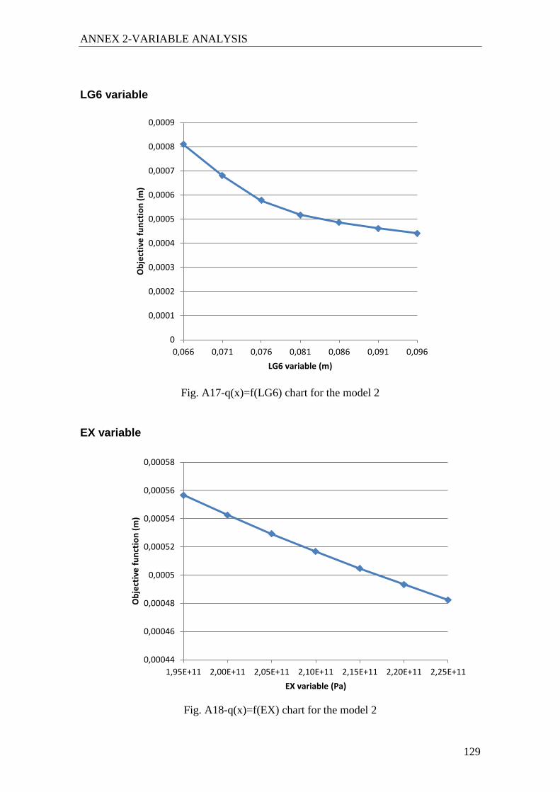
ANNEX 2-VARIABLE ANALYSIS
129
LG6 variable
Fig. A17-q(x)=f(LG6) chart for the model 2
EX variable
Fig. A18-q(x)=f(EX) chart for the model 2
0
0,0001
0,0002
0,0003
0,0004
0,0005
0,0006
0,0007
0,0008
0,0009
0,066 0,071 0,076 0,081 0,086 0,091 0,096
Ob
ject
ive
fu
nct
ion
(m
)
LG6 variable (m)
0,00044
0,00046
0,00048
0,0005
0,00052
0,00054
0,00056
0,00058
1,95E+11 2,00E+11 2,05E+11 2,10E+11 2,15E+11 2,20E+11 2,25E+11
Ob
ject
ive
fu
nct
ion
(m
)
EX variable (Pa)

ANNEX 2-VARIABLE ANALYSIS
130
PXY variable
Fig. A19-q(x)=f(PXY) chart for the model 2
DNS variable
Fig. A20-q(x)=f(DNS) chart for the model 2
0,000495
0,0005
0,000505
0,00051
0,000515
0,00052
0,000525
0,00053
0,23 0,25 0,27 0,29 0,31 0,33 0,35
Ob
ject
ive
fu
nct
ion
(m
)
PXY variable
0
0,0001
0,0002
0,0003
0,0004
0,0005
0,0006
7860 7870 7880 7890 7900 7910 7920
Ob
ejc
tive
fu
nct
ion
(m
)
DNS variable (Kg/m3)

131
ANNEX 3-FINITE ELEMENT MODEL FILES

132

ANNEX 3-FINITE ELEMENT MODEL FILES
133
A3.1-Model 1: ribbed plate ______________________________________________________________________
!/BATCH
! /COM,ANSYS RELEASE 5.4 UP19970828 10:02:38 08/10/2010
/input,start,ans ,C:\ansys54\docu\,,,,,,,,,,,,,,,,1
/PREP7
!
PREX=2.1
PRPXY=2.9
PRDNS=7.89
PRLG1=0.025
PRLG2=0.65
PRLG3=0.46
PRM=15
!
LG1=PRLG1*1
LG2=PRLG2*0.1
LG3=PRLG3*0.01
EX=PREX*1e11
PXY=PRPXY*0.1
DNS=PRDNS*1000
!
K,1,0,-LG2,0,
K,2,0,0,0,
K,3,0.3,-LG2,0,
K,4,0.3,0,0,
!
K,5,0.15-LG1,-LG2,0,
K,6,0.15-LG1,0,0,
K,7,0.15+LG1,-LG2,0
K,8,0.15+LG1,0,0,
!
K,10,0,-LG2,0.6,
K,11,0,0,0.6,
K,12,0.3,-LG2,0.6,
K,13,0.3,0,0.6,
!
K,14,0.15-LG1,-LG2,0.6,
K,15,0.15-LG1,0,0.6,
K,16,0.15+LG1,-LG2,0.6,
K,17,0.15+LG1,0,0.6,
!
K,2014,0.12,0,0.3,
K,2191,0.15,0,0.3,
K,2368,0.18,0,0.3,
!
! /VIEW, 1 ,1,1,1
! /ANG, 1

ANNEX 3-FINITE ELEMENT MODEL FILES
134
! /REP,FAST
K,3000,0.12,0,0.6,
K,4000,0.15,0,0.6,
K,5000,0.18,0,0.6,
K,6000,0.12,0,0,
!
K,7000,0.15,0,0,
K,8000,0.18,0,0,
! /VIEW, 1 ,1,1,1
! /ANG, 1
! /REP,FAST
K,9000,0.3,0,0.3,
K,10000,0.15+LG1,0,0.3,
!
K,11000,0,0,0.3,
K,12000,0.15-LG1,0,0.3,
K,13000,0.15+LG1,-LG2,0.3,
K,14000,0.15-LG1,-LG2,0.3,
!
K,15000,0,-LG2,0.3,
K,16000,0.3,-LG2,0.3,
!
! /REPLOT
! /AUTO, 1
! /REP
! /AUTO, 1
! /REP
! /AUTO, 1
! /REP
! klist,all,,,coord
LSTR, 14, 15
LSTR, 15, 12000
LSTR, 12000, 6
LSTR, 2, 11000
LSTR, 11000, 11
LSTR, 11, 10
LSTR, 10, 1
LSTR, 5, 14
LSTR, 5, 6
LSTR, 1, 2
LSTR, 3000, 2014
LSTR, 2014, 6000
LSTR, 7000, 2191
LSTR, 2191, 4000
LSTR, 5000, 2368
LSTR, 2368, 8000
LSTR, 4, 9000
LSTR, 9000, 13
LSTR, 13, 12
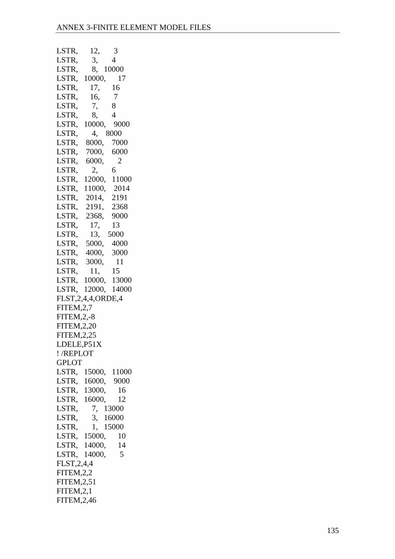
ANNEX 3-FINITE ELEMENT MODEL FILES
135
LSTR, 12, 3
LSTR, 3, 4
LSTR, 8, 10000
LSTR, 10000, 17
LSTR, 17, 16
LSTR, 16, 7
LSTR, 7, 8
LSTR, 8, 4
LSTR, 10000, 9000
LSTR, 4, 8000
LSTR, 8000, 7000
LSTR, 7000, 6000
LSTR, 6000, 2
LSTR, 2, 6
LSTR, 12000, 11000
LSTR, 11000, 2014
LSTR, 2014, 2191
LSTR, 2191, 2368
LSTR, 2368, 9000
LSTR, 17, 13
LSTR, 13, 5000
LSTR, 5000, 4000
LSTR, 4000, 3000
LSTR, 3000, 11
LSTR, 11, 15
LSTR, 10000, 13000
LSTR, 12000, 14000
FLST,2,4,4,ORDE,4
FITEM,2,7
FITEM,2,-8
FITEM,2,20
FITEM,2,25
LDELE,P51X
! /REPLOT
GPLOT
LSTR, 15000, 11000
LSTR, 16000, 9000
LSTR, 13000, 16
LSTR, 16000, 12
LSTR, 7, 13000
LSTR, 3, 16000
LSTR, 1, 15000
LSTR, 15000, 10
LSTR, 14000, 14
LSTR, 14000, 5
FLST,2,4,4
FITEM,2,2
FITEM,2,51
FITEM,2,1
FITEM,2,46

ANNEX 3-FINITE ELEMENT MODEL FILES
136
AL,P51X
FLST,2,4,4
FITEM,2,46
FITEM,2,3
FITEM,2,9
FITEM,2,52
AL,P51X
FLST,2,4,4
FITEM,2,6
FITEM,2,5
FITEM,2,7
FITEM,2,50
AL,P51X
FLST,2,4,4
FITEM,2,4
FITEM,2,10
FITEM,2,49
FITEM,2,7
AL,P51X
FLST,2,4,4
FITEM,2,44
FITEM,2,5
FITEM,2,34
FITEM,2,2
AL,P51X
FLST,2,4,4
FITEM,2,3
FITEM,2,33
FITEM,2,4
FITEM,2,34
AL,P51X
FLST,2,4,4
FITEM,2,43
FITEM,2,35
FITEM,2,5
FITEM,2,11
AL,P51X
FLST,2,4,4
FITEM,2,4
FITEM,2,32
FITEM,2,12
FITEM,2,35
AL,P51X
FLST,2,4,4
FITEM,2,15
FITEM,2,14
FITEM,2,41
FITEM,2,37
AL,P51X
FLST,2,4,4

ANNEX 3-FINITE ELEMENT MODEL FILES
137
FITEM,2,36
FITEM,2,42
FITEM,2,11
FITEM,2,14
AL,P51X
FLST,2,4,4
FITEM,2,12
FITEM,2,31
FITEM,2,13
FITEM,2,36
AL,P51X
FLST,2,4,4
FITEM,2,37
FITEM,2,16
FITEM,2,30
FITEM,2,13
AL,P51X
FLST,2,4,4
FITEM,2,19
FITEM,2,25
FITEM,2,8
FITEM,2,18
AL,P51X
FLST,2,4,4
FITEM,2,24
FITEM,2,23
FITEM,2,45
FITEM,2,20
AL,P51X
FLST,2,4,4
FITEM,2,8
FITEM,2,48
FITEM,2,21
FITEM,2,17
AL,P51X
FLST,2,4,4
FITEM,2,45
FITEM,2,22
FITEM,2,26
FITEM,2,47
AL,P51X
FLST,2,4,4
FITEM,2,39
FITEM,2,18
FITEM,2,28
FITEM,2,23
AL,P51X
FLST,2,4,4
FITEM,2,28
FITEM,2,17

ANNEX 3-FINITE ELEMENT MODEL FILES
138
FITEM,2,27
FITEM,2,22
AL,P51X
FLST,2,4,4
FITEM,2,40
FITEM,2,38
FITEM,2,15
FITEM,2,18
AL,P51X
FLST,2,4,4
FITEM,2,16
FITEM,2,29
FITEM,2,17
FITEM,2,38
AL,P51X
!*
! /VIEW, 1 ,1,1,1
! /ANG, 1
! /REP,FAST
!*
ET,1,SHELL63
!
R,1,LG3,LG3,LG3,LG3, , ,
RMORE, , , ,
!*
!*
UIMP,1,EX, , ,EX,
UIMP,1,DENS, , ,DNS,
UIMP,1,ALPX, , , ,
UIMP,1,REFT, , , ,
UIMP,1,NUXY, , ,PXY,
UIMP,1,PRXY, , , ,
UIMP,1,GXY, , , ,
UIMP,1,MU, , , ,
UIMP,1,DAMP, , , ,
UIMP,1,KXX, , , ,
UIMP,1,C, , , ,
UIMP,1,ENTH, , , ,
UIMP,1,HF, , , ,
UIMP,1,EMIS, , , ,
UIMP,1,QRATE, , , ,
UIMP,1,RSVX, , , ,
UIMP,1,PERX, , , ,
UIMP,1,VISC, , , ,
UIMP,1,SONC, , , ,
!*
TYPE, 1
MAT, 1
REAL, 1
ESYS, 0

ANNEX 3-FINITE ELEMENT MODEL FILES
139
!*
ESIZE,0.02,0,
MSHAPE,0,2D
MSHKEY,1
!*
FLST,5,20,5,ORDE,2
FITEM,5,1
FITEM,5,-20
CM,_Y,AREA
ASEL, , , ,P51X
CM,_Y1,AREA
CHKMSH,'AREA'
CMSEL,S,_Y
!*
AMESH,_Y1
!*
CMDEL,_Y
CMDEL,_Y1
CMDEL,_Y2
!*
FINISH
/SOLU
! KPLOT
FLST,2,1,3,ORDE,1
FITEM,2,2191
FK,P51X,FY,-3528,
FLST,2,1,3,ORDE,1
FITEM,2,2368
FK,P51X,FY,-5120,
FLST,2,1,3,ORDE,1
FITEM,2,2014
FK,P51X,FY,5120,
FLST,2,16,3,ORDE,4
FITEM,2,1
FITEM,2,-8
FITEM,2,10
FITEM,2,-17
DK,P51X, , , ,0,ALL
!
!
! FKLIST, ALL
! FLIST, ALL
/SOLU
FLST,2,899,1,ORDE,2
FITEM,2,1
FITEM,2,-899
FDELE,P51X,ALL
! FKLIST, ALL
!
! /STAT,SOLU

ANNEX 3-FINITE ELEMENT MODEL FILES
140
SOLVE
!*
/POST1
m=PRM
*DIM,VALUE1,,m,1
! RECOLHE VALORES
*GET,U1,NODE,170,U,Y
*GET,U2,NODE,252,U,Y
*GET,U3,NODE,308,U,Y
*GET,U4,NODE,346,U,Y
*GET,U5,NODE,377,U,Y
*GET,U6,NODE,420,U,Y
*GET,U7,NODE,422,U,Y
*GET,U8,NODE,429,U,Y
*GET,U9,NODE,468,U,Y
*GET,U10,NODE,477,U,Y
*GET,U11,NODE,777,U,Y
*GET,U12,NODE,782,U,Y
*GET,U13,NODE,805,U,Y
*GET,U14,NODE,841,U,Y
*GET,U15,NODE,870,U,Y
!
*VFILL,VALUE1(1,1),DATA,U1
*VFILL,VALUE1(2,1),DATA,U2
*VFILL,VALUE1(3,1),DATA,U3
*VFILL,VALUE1(4,1),DATA,U4
*VFILL,VALUE1(5,1),DATA,U5
*VFILL,VALUE1(6,1),DATA,U6
*VFILL,VALUE1(7,1),DATA,U7
*VFILL,VALUE1(8,1),DATA,U8
*VFILL,VALUE1(9,1),DATA,U9
*VFILL,VALUE1(10,1),DATA,U10
*VFILL,VALUE1(11,1),DATA,U11
*VFILL,VALUE1(12,1),DATA,U12
*VFILL,VALUE1(13,1),DATA,U13
*VFILL,VALUE1(14,1),DATA,U14
*VFILL,VALUE1(15,1),DATA,U15
!*
/output,n5,lgw,d:\abc
*VWRITE,VALUE1(1,1)
(1X,F10.8)
/output
!*
______________________________________________________________________
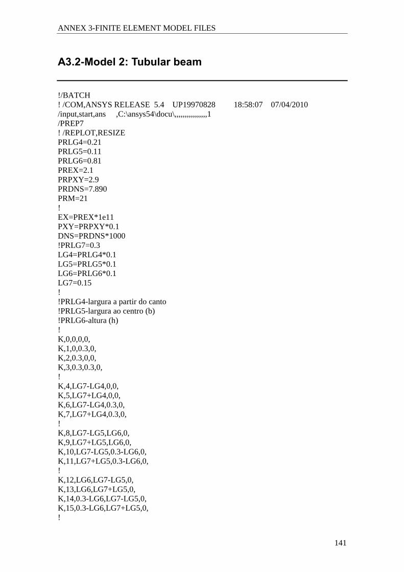
ANNEX 3-FINITE ELEMENT MODEL FILES
141
A3.2-Model 2: Tubular beam
!/BATCH
! /COM,ANSYS RELEASE 5.4 UP19970828 18:58:07 07/04/2010
/input,start,ans ,C:\ansys54\docu\,,,,,,,,,,,,,,,,1
/PREP7
! /REPLOT,RESIZE
PRLG4=0.21
PRLG5=0.11
PRLG6=0.81
PREX=2.1
PRPXY=2.9
PRDNS=7.890
PRM=21
!
EX=PREX*1e11
PXY=PRPXY*0.1
DNS=PRDNS*1000
!PRLG7=0.3
LG4=PRLG4*0.1
LG5=PRLG5*0.1
LG6=PRLG6*0.1
LG7=0.15
!
!PRLG4-largura a partir do canto
!PRLG5-largura ao centro (b)
!PRLG6-altura (h)
!
K,0,0,0,0,
K,1,0,0.3,0,
K,2,0.3,0,0,
K,3,0.3,0.3,0,
!
K,4,LG7-LG4,0,0,
K,5,LG7+LG4,0,0,
K,6,LG7-LG4,0.3,0,
K,7,LG7+LG4,0.3,0,
!
K,8,LG7-LG5,LG6,0,
K,9,LG7+LG5,LG6,0,
K,10,LG7-LG5,0.3-LG6,0,
K,11,LG7+LG5,0.3-LG6,0,
!
K,12,LG6,LG7-LG5,0,
K,13,LG6,LG7+LG5,0,
K,14,0.3-LG6,LG7-LG5,0,
K,15,0.3-LG6,LG7+LG5,0,
!

ANNEX 3-FINITE ELEMENT MODEL FILES
142
K,16,0,LG7-LG4,0,
K,17,0.3,LG7-LG4,0,
K,18,0,LG7+LG4,0,
K,19,0.3,LG7+LG4,0,
K,20,0,0,0,
!
K,100,0,0,1,
K,101,0,0.3,1,
K,102,0.3,0,1,
K,103,0.3,0.3,1,
!
K,104,LG7-LG4,0,1,
K,105,LG7+LG4,0,1,
K,106,LG7-LG4,0.3,1,
K,107,LG7+LG4,0.3,1,
!
K,108,LG7-LG5,LG6,1,
K,109,LG7+LG5,LG6,1,
K,110,LG7-LG5,0.3-LG6,1,
K,111,LG7+LG5,0.3-LG6,1,
!
K,112,LG6,LG7-LG5,1,
K,113,LG6,LG7+LG5,1,
K,114,0.3-LG6,LG7-LG5,1,
K,115,0.3-LG6,LG7+LG5,1,
!
K,116,0,LG7-LG4,1,
K,117,0.3,LG7-LG4,1,
K,118,0,LG7+LG4,1,
K,119,0.3,LG7+LG4,1,
!
K,1000,0.15,0.3-LG6,0,
K,2000,0.15,0.3-LG6,1,
K,3000,LG7-LG5,0.3-LG6,0.5,
K,4000,0.15,0.3-LG6,0.5,
!
K,5000,LG7+LG5,0.3-LG6,0.5,
K,6000,0,0,0.5,
K,7000,0,0.3,0.5,
K,8000,0.3,0,0.5,
!
K,9000,0.3,0.3,0.5,
K,10000,LG7-LG4,0,0.5,
K,11000,LG7+LG4,0,0.5,
K,12000,LG7-LG4,0.3,0.5,
!
K,13000,LG7+LG4,0.3,0.5,
K,14000,LG7-LG5,LG6,0.5,
K,15000,LG7+LG5,LG6,0.5,
K,16000,LG6,LG7-LG5,0.5,

ANNEX 3-FINITE ELEMENT MODEL FILES
143
!
K,17000,LG6,LG7+LG5,0.5,
K,18000,0.3-LG6,LG7-LG5,0.5,
K,19000,0.3-LG6,LG7+LG5,0.5,
K,20000,0,LG7-LG4,0.5,
!
K,21000,0.3,LG7-LG4,0.5,
K,22000,0.3,LG7+LG4,0.5,
K,23000,0,LG7+LG4,0.5,
!
! /VIEW, 1 ,1,1,1
! /ANG, 1
! /REP,FAST
LSTR, 101, 118
LSTR, 118, 113
LSTR, 113, 112
LSTR, 112, 116
LSTR, 116, 100
LSTR, 100, 104
LSTR, 104, 108
LSTR, 108, 109
LSTR, 109, 105
LSTR, 105, 102
LSTR, 102, 117
LSTR, 117, 114
LSTR, 114, 115
LSTR, 115, 119
LSTR, 119, 103
LSTR, 103, 107
LSTR, 107, 111
LSTR, 111, 2000
LSTR, 2000, 110
LSTR, 110, 106
LSTR, 106, 101
LSTR, 7000, 23000
LSTR, 23000, 17000
LSTR, 17000, 16000
LSTR, 16000, 20000
LSTR, 20000, 6000
LSTR, 6000, 10000
LSTR, 10000, 14000
LSTR, 14000, 15000
LSTR, 15000, 11000
LSTR, 11000, 8000
LSTR, 8000, 21000
LSTR, 21000, 18000
LSTR, 18000, 19000
LSTR, 19000, 22000
LSTR, 22000, 9000
LSTR, 9000, 13000
ANNEX 3-FINITE ELEMENT MODEL FILES
144
LSTR, 13000, 5000
LSTR, 5000, 4000
LSTR, 4000, 3000
LSTR, 3000, 12000
LSTR, 12000, 7000
LSTR, 1, 18
LSTR, 18, 13
LSTR, 13, 12
LSTR, 12, 16
LSTR, 16, 20
LSTR, 20, 4
LSTR, 4, 8
LSTR, 8, 9
LSTR, 9, 5
LSTR, 5, 2
LSTR, 2, 17
LSTR, 17, 14
LSTR, 14, 15
LSTR, 15, 19
LSTR, 19, 3
LSTR, 3, 7
LSTR, 7, 11
LSTR, 11, 1000
LSTR, 1000, 10
LSTR, 10, 6
LSTR, 6, 1
LSTR, 101, 7000
LSTR, 7000, 1
LSTR, 118, 23000
LSTR, 23000, 18
LSTR, 113, 17000
LSTR, 17000, 13
LSTR, 112, 16000
LSTR, 16000, 12
LSTR, 116, 20000
LSTR, 20000, 16
LSTR, 100, 6000
LSTR, 6000, 20
LSTR, 104, 10000
LSTR, 10000, 4
LSTR, 108, 14000
LSTR, 14000, 8
LSTR, 109, 15000
LSTR, 15000, 9
LSTR, 105, 11000
LSTR, 11000, 5
LSTR, 102, 8000
LSTR, 8000, 2
LSTR, 117, 21000
LSTR, 21000, 17
ANNEX 3-FINITE ELEMENT MODEL FILES
145
LSTR, 114, 18000
LSTR, 18000, 14
LSTR, 115, 19000
LSTR, 19000, 15
LSTR, 119, 22000
LSTR, 22000, 19
LSTR, 103, 9000
LSTR, 9000, 3
LSTR, 107, 13000
LSTR, 13000, 7
LSTR, 111, 5000
LSTR, 5000, 11
LSTR, 2000, 4000
LSTR, 4000, 1000
LSTR, 110, 3000
LSTR, 3000, 10
LSTR, 106, 12000
LSTR, 12000, 6
FLST,2,4,4
FITEM,2,6
FITEM,2,74
FITEM,2,27
FITEM,2,76
AL,P51X
FLST,2,4,4
FITEM,2,5
FITEM,2,72
FITEM,2,26
FITEM,2,74
AL,P51X
FLST,2,4,4
FITEM,2,4
FITEM,2,70
FITEM,2,25
FITEM,2,72
AL,P51X
FLST,2,4,4
FITEM,2,3
FITEM,2,68
FITEM,2,24
FITEM,2,70
AL,P51X
FLST,2,4,4
FITEM,2,2
FITEM,2,66
FITEM,2,23
FITEM,2,68
AL,P51X
FLST,2,4,4
FITEM,2,1

ANNEX 3-FINITE ELEMENT MODEL FILES
146
FITEM,2,64
FITEM,2,22
FITEM,2,66
AL,P51X
FLST,2,4,4
FITEM,2,21
FITEM,2,64
FITEM,2,42
FITEM,2,104
AL,P51X
FLST,2,4,4
FITEM,2,20
FITEM,2,102
FITEM,2,41
FITEM,2,104
AL,P51X
FLST,2,4,4
FITEM,2,19
FITEM,2,102
FITEM,2,40
FITEM,2,100
AL,P51X
FLST,2,4,4
FITEM,2,100
FITEM,2,18
FITEM,2,98
FITEM,2,39
AL,P51X
FLST,2,4,4
FITEM,2,98
FITEM,2,17
FITEM,2,96
FITEM,2,38
AL,P51X
LSTR, 103, 9000
! LPLOT
FLST,2,4,4
FITEM,2,94
FITEM,2,16
FITEM,2,96
FITEM,2,37
AL,P51X
GPLOT
FLST,2,4,4
FITEM,2,94
FITEM,2,15
FITEM,2,36
FITEM,2,92
AL,P51X
FLST,2,4,4

ANNEX 3-FINITE ELEMENT MODEL FILES
147
FITEM,2,14
FITEM,2,90
FITEM,2,35
FITEM,2,92
AL,P51X
FLST,2,4,4
FITEM,2,7
FITEM,2,78
FITEM,2,28
FITEM,2,76
AL,P51X
FLST,2,4,4
FITEM,2,8
FITEM,2,78
FITEM,2,29
FITEM,2,80
AL,P51X
FLST,2,4,4
FITEM,2,9
FITEM,2,80
FITEM,2,30
FITEM,2,82
AL,P51X
FLST,2,4,4
FITEM,2,10
FITEM,2,82
FITEM,2,31
FITEM,2,84
AL,P51X
FLST,2,4,4
FITEM,2,11
FITEM,2,86
FITEM,2,32
FITEM,2,84
AL,P51X
FLST,2,4,4
FITEM,2,12
FITEM,2,88
FITEM,2,33
FITEM,2,86
AL,P51X
FLST,2,4,4
FITEM,2,13
FITEM,2,88
FITEM,2,34
FITEM,2,90
AL,P51X
! /ANG, 1 ,-30.000000,YS,1
! /REP,FAST
! /ANG, 1 ,30.000000,YS,1

ANNEX 3-FINITE ELEMENT MODEL FILES
148
! /REP,FAST
! /ANG, 1 ,30.000000,YS,1
! /REP,FAST
! /VIEW, 1 ,1,1,1
! /ANG, 1
! /REP,FAST
FLST,2,4,4
FITEM,2,22
FITEM,2,65
FITEM,2,43
FITEM,2,67
AL,P51X
FLST,2,4,4
FITEM,2,23
FITEM,2,67
FITEM,2,44
FITEM,2,69
AL,P51X
FLST,2,4,4
FITEM,2,24
FITEM,2,69
FITEM,2,45
FITEM,2,71
AL,P51X
FLST,2,4,4
FITEM,2,25
FITEM,2,73
FITEM,2,46
FITEM,2,71
AL,P51X
FLST,2,4,4
FITEM,2,26
FITEM,2,73
FITEM,2,47
FITEM,2,75
AL,P51X
FLST,2,4,4
FITEM,2,27
FITEM,2,75
FITEM,2,48
FITEM,2,77
AL,P51X
FLST,2,4,4
FITEM,2,28
FITEM,2,77
FITEM,2,49
FITEM,2,79
AL,P51X
FLST,2,4,4
FITEM,2,29

ANNEX 3-FINITE ELEMENT MODEL FILES
149
FITEM,2,79
FITEM,2,50
FITEM,2,81
AL,P51X
FLST,2,4,4
FITEM,2,30
FITEM,2,81
FITEM,2,51
FITEM,2,83
AL,P51X
FLST,2,4,4
FITEM,2,32
FITEM,2,87
FITEM,2,53
FITEM,2,85
AL,P51X
FLST,2,4,4
FITEM,2,33
FITEM,2,89
FITEM,2,54
FITEM,2,87
AL,P51X
FLST,2,4,4
FITEM,2,34
FITEM,2,55
FITEM,2,89
FITEM,2,91
AL,P51X
FLST,2,4,4
FITEM,2,35
FITEM,2,93
FITEM,2,56
FITEM,2,91
AL,P51X
FLST,2,4,4
FITEM,2,36
FITEM,2,95
FITEM,2,57
FITEM,2,93
AL,P51X
FLST,2,4,4
FITEM,2,37
FITEM,2,95
FITEM,2,58
FITEM,2,97
AL,P51X
FLST,2,4,4
FITEM,2,42
FITEM,2,65
FITEM,2,63

ANNEX 3-FINITE ELEMENT MODEL FILES
150
FITEM,2,105
AL,P51X
FLST,2,4,4
FITEM,2,41
FITEM,2,103
FITEM,2,62
FITEM,2,105
AL,P51X
FLST,2,4,4
FITEM,2,40
FITEM,2,103
FITEM,2,61
FITEM,2,101
AL,P51X
FLST,2,4,4
FITEM,2,39
FITEM,2,60
FITEM,2,101
FITEM,2,99
AL,P51X
FLST,2,4,4
FITEM,2,38
FITEM,2,99
FITEM,2,59
FITEM,2,97
AL,P51X
!
! /VIEW, 1 ,1,1,1
! /ANG, 1
! /REP,FAST
!*
ET,1,SHELL63
!*
!*
R,1,0.002,0.002,0.002,0.002, , ,
RMORE, , , ,
!*
!*
UIMP,1,EX, , ,EX,
UIMP,1,DENS, , ,DNS,
UIMP,1,ALPX, , , ,
UIMP,1,REFT, , , ,
UIMP,1,NUXY, , ,PXY,
UIMP,1,PRXY, , , ,
UIMP,1,GXY, , , ,
UIMP,1,MU, , , ,
UIMP,1,DAMP, , , ,
UIMP,1,KXX, , , ,
UIMP,1,C, , , ,
UIMP,1,ENTH, , , ,

ANNEX 3-FINITE ELEMENT MODEL FILES
151
UIMP,1,HF, , , ,
UIMP,1,EMIS, , , ,
UIMP,1,QRATE, , , ,
UIMP,1,RSVX, , , ,
UIMP,1,PERX, , , ,
UIMP,1,VISC, , , ,
UIMP,1,SONC, , , ,
!*
TYPE, 1
MAT, 1
REAL, 1
ESYS, 0
!*
ESIZE,0.05,0,
ESIZE,0.02,0,
MSHAPE,0,2D
MSHKEY,1
!*
FLST,5,41,5,ORDE,2
FITEM,5,1
FITEM,5,-41
CM,_Y,AREA
ASEL, , , ,P51X
CM,_Y1,AREA
CHKMSH,'AREA'
CMSEL,S,_Y
!*
AMESH,_Y1
!*
CMDEL,_Y
CMDEL,_Y1
CMDEL,_Y2
!*
FINISH
/SOLU
! KPLOT
FLST,2,1,3,ORDE,1
FITEM,2,4000
FK,P51X,FY,-3528,
FLST,2,1,3,ORDE,1
FITEM,2,5000
FK,P51X,FY,-5120,
FLST,2,1,3,ORDE,1
FITEM,2,3000
FK,P51X,FY,5120,
FLST,2,40,3,ORDE,4
FITEM,2,1
FITEM,2,-20
FITEM,2,100
FITEM,2,-119

ANNEX 3-FINITE ELEMENT MODEL FILES
152
DK,P51X, , , ,0,ALL
! /STAT,SOLU
SOLVE
! /REPLOT,RESIZE
! LGWRITE,vigatub_original,lgw,..\..\MATLAB6p5\work\,COMMENT
!
m=PRM
*DIM,VALUE1,,m,1
*GET,U1,NODE,625,U,Y
!
*GET,U2,NODE,629,U,Y
*GET,U3,NODE,640,U,Y
*GET,U4,NODE,649,U,Y
*GET,U5,NODE,833,U,Y
*GET,U6,NODE,835,U,Y
*GET,U7,NODE,844,U,Y
*GET,U8,NODE,854,U,Y
*GET,U9,NODE,941,U,Y
*GET,U10,NODE,948,U,Y
*GET,U11,NODE,957,U,Y
*GET,U12,NODE,965,U,Y
*GET,U13,NODE,3378,U,Y
*GET,U14,NODE,3385,U,Y
*GET,U15,NODE,3394,U,Y
*GET,U16,NODE,3478,U,Y
*GET,U17,NODE,3489,U,Y
*GET,U18,NODE,3497,U,Y
*GET,U19,NODE,3678,U,Y
*GET,U20,NODE,3687,U,Y
*GET,U21,NODE,3695,U,Y
!
*VFILL,VALUE1(1,1),DATA,U1
*VFILL,VALUE1(2,1),DATA,U2
*VFILL,VALUE1(3,1),DATA,U3
*VFILL,VALUE1(4,1),DATA,U4
*VFILL,VALUE1(5,1),DATA,U5
*VFILL,VALUE1(6,1),DATA,U6
*VFILL,VALUE1(7,1),DATA,U7
*VFILL,VALUE1(8,1),DATA,U8
*VFILL,VALUE1(9,1),DATA,U9
*VFILL,VALUE1(10,1),DATA,U10
*VFILL,VALUE1(11,1),DATA,U11
*VFILL,VALUE1(12,1),DATA,U12
*VFILL,VALUE1(13,1),DATA,U13
*VFILL,VALUE1(14,1),DATA,U14
*VFILL,VALUE1(15,1),DATA,U15
*VFILL,VALUE1(16,1),DATA,U16
*VFILL,VALUE1(17,1),DATA,U17

ANNEX 3-FINITE ELEMENT MODEL FILES
153
*VFILL,VALUE1(18,1),DATA,U18
*VFILL,VALUE1(19,1),DATA,U19
*VFILL,VALUE1(20,1),DATA,U20
*VFILL,VALUE1(21,1),DATA,U21
!*
/output,n5,lgw,d:\abc
*VWRITE,VALUE1(1,1)
(1X,F10.8)
/output
!*
FINISH
!*
!/EXIT
______________________________________________________________________

154

155
ANNEX 4-SCIENTIFIC PAPER

156

ANNEX 4-SCIENTIFIC PAPER
157
Determination of material/geometry of the section most adequate for a static loaded beam subjected to a combination
of bending and torsion
Hugo Miguel Silva1, a, José Filipe Meireles1,b 1 Department of Mechanical Engineering, University of Minho, campus de Azurém,
4800-058 Guimarães, Portugal
[email protected] (corresponding author), [email protected], Keywords: Finite Element Method, Finite Element Model Updating, Optimization, MATLAB, ANSYS, Structural Static Analysis, Materials Selection, Strength
Abstract. The acceleration of industrial machines mobile parts has been increasing over
the last few years, due to the need of higher production in a short period of time. The
machines were dimensioned for a lower value of acceleration, which means there is not
enough rigidity for the correct operation at much higher accelerations. Nowadays, the
accelerations can be near 12 times the acceleration of gravity. There is the need of
improving rigidity to make possible the correct machine operation without undesired
vibrations that can ultimately lead to failure. The main applications of this work are
plotters and laser cutting machines. To improve rigidity, one must improve the relevant
material properties, and the relevant geometric variables of the model.[1] A novel Finite
Element Model Updating methodology is presented in this paper. The considered
models were : a ribbed plate and a tubular beam. The models were built by means of the
Finite Element Method (FEM), and MATLAB was used to control the optimization
process, using a programming code. Both material properties and geometric parameters
were optimized. The main aim of the materials modeling is to know how the value of
the objective function changes with the value of the material properties. Materials
selection was performed, using material selection charts, to select the best material for
the application. The value of these properties was not in the catalogue, and the
properties used to perform the material selection were related to a material sub-class,
Eg. Steel. The final material selection determined the best specific material for the
application, and that material was mechanically tested. The mechanical tests performed
were: Tensile Test and Extensometry Test, to obtain the relevant material properties,
mainly Young Modulus, Poisson Coefficient and Yield Stress. The deflection of the
optimized models reduced strongly in comparison to the initial models.
1. Introduction
This paper consists mainly in the development and analysis of a finite element model
updating application for structural static analysis to reduce the models deflections to a
minimum when subjected to static bending and torsion combined loads. To achieve the
aim of deflection reduction, one must optimize both geometric parameters and material
properties, focusing two main factors: The Young Modulus and the Inertia Moment,
with the goal of maximizing the rigidity and minimizing the object mass. The Young
Modulus is only dependent of the chosen material, and the Inertia Moment is highly
dependent of the geometric characteristics of the object. Rigidity is very important in
what relates to engineering parts, because it determines the work capability of
engineering industrial equipments. The importance of rigidity can be higher than
resistance in what relates to equipment reliability.[1] The use of numeric methods of
calculus, such as the Finite Element Method (FEM), controlled by optimization

ANNEX 4-SCIENTIFIC PAPER
158
processes that can help the designer in the most adequate selection between the existing
valid solutions can be very useful.
2. Bending and torsion combined load
In practice is very common to find situations where the structural parts are loaded with a
combination of bending and torsion. Bending is usually due to moments or centered
transverse loads, and torsion can be due to non-centered transverse load. In some
situations, these two types of loads act at the same time, and so, one have a combination
of bending and torsion. In bending there are only normal stresses, and in torsion there
are only shear stresses.
The deflection due to bending can be calculated by (1): 2
2 48
bd y PL
EIdx .
(1)
The models in this work are simply supported at its ends. For this type of support, the
bending deflection due to transverse load can be obtained by (2): 3 2 3
2 3
3 4*( ).
48b
PL x xy
EI L L
(2)
where:
yb is the deflection due to bending, P is the applied load, L is the beam´s length, E is the
Young Modulus, I is the axial inertia moment, x is the x coordinate
In a similar manner, the maximum distortion angle for hollow-box beams of low
thickness subjected to torsion is (3):
2
0 0
.4 2
tM M CM
GA t GA t
(3)
where:
is the twist angle, C is the shear flux, M is the mean line perimeter, G is the
transversal elasticity modulus,A0 is the mean line area, t is the object thickness, Mt is
the torsion moment
The deflection due to torsion can be calculated by (4):
.2
t
Dy L
(4)
where:
yt is the deflection due to torsion, D is the diagonal length of the object
The total deflection can be expressed as the sum of the contributions of bending and
torsion (5):
.total b ty y y
(5)
In a bending and torsion combined load, the resulting deflection is a consequence of the
combination of the normal stresses due to bending and the shear stresses due to
torsion.[2,3]

ANNEX 4-SCIENTIFIC PAPER
159
3. The FEM models
In order to validate the Finite Element Model Updating methodology done during this
work two models were built: a ribbed plate, named model one and a tubular beam,
named model two. In both models one considered three geometric variables and three
material properties variables. Due to the different nature of the two objects the
geometric variables are different in the two models. However, the material properties
were the same in the two models: Poisson coefficient, Density and Young Modulus. The
variables of the FEM models are in the table 1(ribbed plate) and in the table 2(tubular
beam). The figure 1 and 2 shows the areas of the FEM models, as well as its variables:
Fig.1-Areas (left) and variables (right) of the ribbed plate FEM model
Variables of the ribbed plate FEM model
Geometric variables Material properties
LG1 Distance of inner ribs to the center EX Young modulus
LG2 Rib Height PXY Poisson coefficient
LG3 Thickness DNS Density
Table 1- Variables of the ribbed plate FEM model
Fig.2-Areas (left) and variables (right) of the tubular beam FEM model
Variables of the tubular beam FEM model
Geometric variables Material properties
LG4 Center to corner segment distance EX Young modulus
LG5 Half width of the central segment PXY Poisson coefficient
LG6 Height of the central part on the wall DNS Density
Table 2- Variables of the tubular beam FEM model

ANNEX 4-SCIENTIFIC PAPER
160
4. Optimization Model
The MATLAB program is used together with ANSYS. MATLAB controls the
optimization process and ANSYS solves the FEM problem, by sending the deflections
in specific nodes to a text file, that MATLAB can read. Then MATLAB calculates a
new objective function value, changes variable values and sends orders to ANSYS to
recalculate the deflections for the new variable values. The objective function q(U) can
be defined as:
( ) ( )q U ABS Ui (5)
where:
q(U) is the objective function, Ui is the deflection on each nodal points (nodes),ABS is
absolute value of an argument.
The objective function q(U) was minimized by a MATLAB function named fmincon
(nonlinear minimization). The objective function value is better the closer it is to zero.
The figure 3 shows the interaction between ANSYS and the MATLAB optimization
program:
Fig.3-Functional fluxogram of the optimization methodology [4]
5. Materials selection
The first step in the materials selection is the definition of the relevant properties for the
application. In this work, the desired properties are (Table3):
Relevant properties for the materials selection
- Young modulus (highest possible) - Toughness (highest possible) - Cost of the material (lowest possible)
- Density (lowest possible)
Table 3- Desired properties for materials selection
For the initial materials selection it is necessary to choose a material class, not a specific
material, because one has more mobility to change to another material in the same class
with better properties for the application. The materials selection was performed using
the Young Modulus/Density and Young Modulus/Cost materials selection charts
(Fig.4).

ANNEX 4-SCIENTIFIC PAPER
161
Fig.4-Materials selection charts Young Modulus/Density (left)
and Young Modulus/Cost (right) [5]
In both charts(fig.4), the best classes are the ceramics, the composites with high Young
Modulus and the metals. The ceramics are too brittle for this application. The
composites with high Young Modulus are expensive (Eg. CFRP- Carbon Fiber
Reinforced Polymer). The cheaper Composites have a low density but a lower Young
Modulus than Metals. The Metals have a high Toughness and high Young Modulus.
Some Composites have a low density and high Young Modulus, but their cost is much
higher, so they are not the best choice. The best material class is the Metals and Alloys,
which is the best class in both charts. In a detailed view of the Density/Young modulus
diagram (fig.4), one can see that the best materials for this application are: Steel, Cast
Iron and Nickel, whose have a high Young Modulus and a relatively low density,
compared with some metals, such as Gold or Lead. A detailed view of the diagram
Cost/Young modulus (fig.4) shows that the best materials for this application are: Low
alloy Steels and Stainless Steel, whose have a high Young modulus and a relatively low
cost. One can say that the best material for this application is the Steel, which has a
good position in both diagrams. Of all steels, the dual-phase steels seem to be the most
promising material for this application. Dual phase steels allows decreasing the objects
thickness and improving the inertia moment of the section to obtain lower deflections
with a similar material cost. The dual phase steel has high yield stress, which means it
can be subjected to high loads without entering the plastic domain. The commercial
dual phase steel DOCOL is the selected material.
6 Results
6.1 Tensile test results
In order to determine Young Modulus, one must plot the Stress-Strain chart of the
elastic domain only, and do a linear fit to find the slope of the recta. The Yield Stress
was calculated using a 0,2% offset. The obtained Young Modulus and Yield Stress is
shown on the table 4:
Young Modulus and Yield Stress obtained in tensile test
Specimen number Specimen designation Young Modulus Value Yield Stress value
Specimen 1 DOCOL 600 DL Long 193,2 [GPa] 309,12 [MPa]
Specimen 2 DOCOL 800 DP Long 168,2 [GPa] 555,06 [MPa]
Table 4- Young modulus and Yield Stress obtained in the extensometry test

ANNEX 4-SCIENTIFIC PAPER
162
6.2 Extensometry test results
The table 5 shows the Young Modulus range and the mean Poisson coefficient for the
four specimens tested by extensometry test:
Poisson coefficient and Young Modulus obtained in Extensometry test
Specimen number Specimen designation Poisson coefficient Young modulus
Specimen 3 DOCOL 600 DL Trans 0,285 182-198 [GPa]
Specimen 4 DOCOL 600 DL Long 0,284 176-186 [GPa]
Specimen 5 DOCOL 800 DP Trans 0,287 186-192 [GPa]
Specimen 6 DOCOL 800 DP Long 0,270 184-203 [GPa]
Table 5- Poisson coefficient and Young modulus obtained in the extensometry
test.
6.3 Optimization results
The final variable values for the ribbed plate model are shown in the table 6. The final
value of the objective function was: q(x)=0,00092 for the geometric parameters
optimization and q(x)=0,04258 for the material properties optimization.
Final variable values for the ribbed plate model
Geometric parameters optimization Material properties optimization
Variable Initial
Value[m]
Final
Value[m] Variable Initial Value Final Value
LG1 0,100 0,025 EX 2,1*1011
[Pa] 2,31*1011
[Pa]
LG2 0,03 0,0507 PXY 0,29 0,435
LG3 0,002 0,0046 DNS 7890 [Kg/m3] 7890 [Kg/m
3]
Table 6-Final variable values for the geometric parameters optimization (ribbed plate)
The final variable values for the tubular beam model are shown in the table 7. The final
value of the objective function was: q(x)=0,00053 for the geometric parameters
optimization and q(x)=0,01151 for the material properties optimization.
Final variable values for the tubular beam model
Geometric parameters optimization Material properties optimization
Variable Initial
Value[m]
Final
Value[m] Variable
Initial
Value[m] Final Value
LG4 0,085 0,0213 EX 2,1*1011
[Pa] 2,31*1011
[Pa]
LG5 0,030 0,0076 PXY 0,29 0,292
LG6 0,035 0,0805 DNS 7890 [Kg/m3] 7890 [Kg/m
3]
Table 7-Final variable values for the material properties optimization (tubular
beam)
7. Results discussion and conclusions
In tensile test, the specimen 1 has the highest Young Modulus of the two specimens
tested: 193,2 GPa. The specimen 2 has a Young Modulus of near 168,2 GPa. The
Young Modulus obtained by extensometry test ranged from near 180 to 200 GPa. The

ANNEX 4-SCIENTIFIC PAPER
163
Young Modulus values are lower than the regular value of the steel, which is 210 GPa.
The manufacturing processes may be the reason of such values of Young Modulus,
because the material is conformed, and as a result of the increase in plasticity, the
Young Modulus may decrease. The Specimen 1 has a lower Yield Stress, which is
expected, because its designation is 600 and the specimen 2 is 800. This number is
related to the Yield Stress in relative terms, which means that a lower number
designation means a lower Yield Stress when comparing two specimens. The obtained
Poisson Coefficient in extensometry test was near 0,29, which is the normal value for a
steel, except for the specimen 6, which was near 0,27. About the optimization results,
the obtained objective function is lower in the geometric parameters optimization than
in the material properties optimization for both models. The conclusions of this work
are: the developed Finite Element Model Updating code can be successfully used to
optimize both geometric parameters and material properties. The geometric parameters
play a more important role in the optimization process than the material properties,
because the obtained objective function is lower in the geometric parameters
optimization than in the material properties optimization. The tested specimens have
high Yield Stresses, which means the material can be subjected to high loads before
entering the plastic domain. In the practical applications of this work (plotters and laser
cutting machines) it is very important to ensure that the material doesn´t leave the
elastic domain, otherwise the permanent deformation will negatively affect the machine
operation. Considering this fact, the dual phase steels are an adequate material for the
applications of this work. The selected material does not reduce the deflections, because
it has a lower Young Modulus, but the deflections can be substantially improved by the
optimization of the geometry.
References
[1] C. M. Branco, J. M. Ferreira, J. D. Costa, A. S. Ribeiro, Projecto de Órgãos de
Máquinas, Fundação Calouste Gulbenkian, Lisboa, Portugal, 2005.
[2] F. Beer, Johnston, De Wolf, “Mechanics of Materials, McGraw Hill, Third Edition,
2001
[3] C. Massonnet,”Resistance des matériaux”, DUNOD,deuxiéme édition, Paris, 1968
[4] J. F. B. Meireles,”Análise dinâmica de estruturas por modelos de elementos finitos
identificados experimentalmente”, Ph.D. Thesis, University of Minho,2007
[5] Information on http://www.materials.eng.cam.ac.uk/mpsite/interactive_charts
/default.html


![Untitled-1 [] · Title: Untitled-1 Author: Pedro Figueiredo Created Date: 20161203104633Z](https://img.pdfslide.us/doc/110x75/5bed0a7709d3f26e208cf593/untitled-1-title-untitled-1-author-pedro-figueiredo-created-date-20161203104633z.jpg)