Embed Size (px)
Citation preview
DA Training Course 2014
Variational Quality Control
Elias Holm
Data Assimilation Section, ECMWF
Contributors: Lars Isaksen, Christina Tavolato,Erik Andersson and Elias Holm, ECMWF
1

Outline of Lecture
Introduction
VarQC formulation 1: Gaussian+constant
Rejection limits and tuning
VarQC formulation 2: Huber norm
Example
Summary
DA Training Course 2014 2
DA Training Course 2014
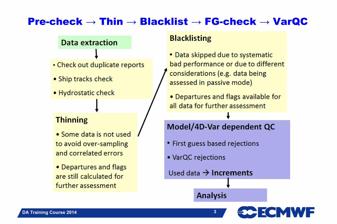
Pre-check → Thin → Blacklist → FG-check → VarQC
3

DA Training Course 2014
Weight of observations in the analysis
Assuming Gaussian statistics, the maximum likelihood solution to the linear estimation problem results in observation analysis weights (w) that are independent of the observed value.
22
2
)(
bo
b
bba
w
Hxywxx
Outliers will be given the same weight as good data, potentially corrupting the analysis
4

DA Training Course 2014
Even good-quality data show significant deviations from the pure Gaussian form
“Tail”QC-rejection or
good data?
Actual distribution
K
The real data distribution has fatter tails than the Gaussian
Aircraft temperature observations shown here
Gaussian
obs-bg departures
5
DA Training Course 2014
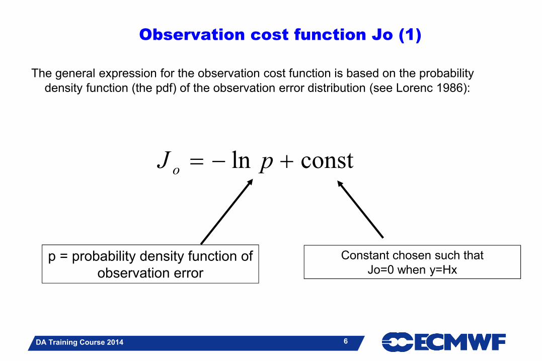
The general expression for the observation cost function is based on the probability density function (the pdf) of the observation error distribution (see Lorenc 1986):
constln pJ o
p = probability density function of observation error
Constant chosen such thatJo=0 when y=Hx
Observation cost function Jo (1)
6
DA Training Course 2014
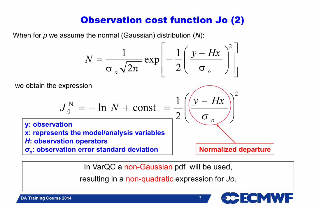
When for p we assume the normal (Gaussian) distribution (N):
2
N0
2
1constln
o
HxyNJ
2
2
1exp
2
1
oo
HxyN
we obtain the expression
In VarQC a non-Gaussian pdf will be used,
resulting in a non-quadratic expression for Jo.
Observation cost function Jo (2)
y: observationx: represents the model/analysis variablesH: observation operatorsσo: observation error standard deviation Normalized departure
7
DA Training Course 2014
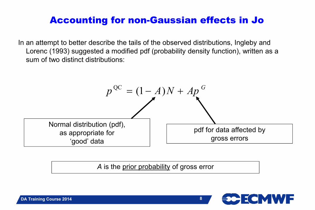
Accounting for non-Gaussian effects in Jo
In an attempt to better describe the tails of the observed distributions, Ingleby and Lorenc (1993) suggested a modified pdf (probability density function), written as a sum of two distinct distributions:
GApNAp )1(QC
A is the prior probability of gross error
Normal distribution (pdf),as appropriate for
‘good’ data
pdf for data affected bygross errors
8
DA Training Course 2014
-70 -60 -50 -40 -30 -20 -10 0 10 20 30
OBS TEMPERATURE (C)
-10
-9
-8
-7
-6
-5
-4
-3
-2
-1
0
1
2
3
4
5
6
7
8
9
10
OB
S -
FG
1
3
6
11
20
36
66
121
OB
S -
FG
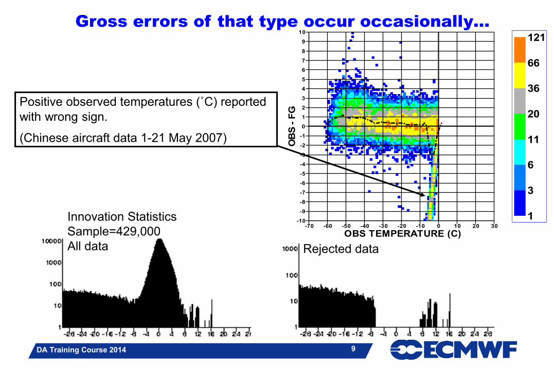
Innovation StatisticsSample=429,000All data
Positive observed temperatures (˚C) reported with wrong sign.
(Chinese aircraft data 1-21 May 2007)
Gross errors of that type occur occasionally…
Rejected data
9
DA Training Course 2014
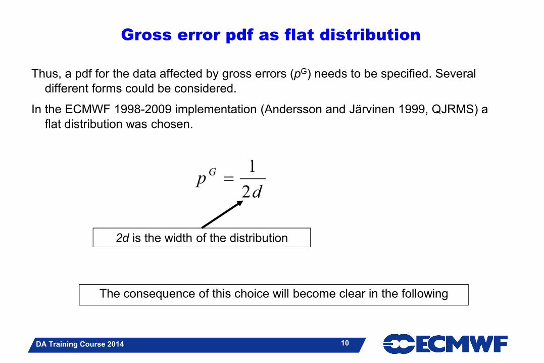
Gross error pdf as flat distribution
Thus, a pdf for the data affected by gross errors (pG) needs to be specified. Several different forms could be considered.
In the ECMWF 1998-2009 implementation (Andersson and Järvinen 1999, QJRMS) a flat distribution was chosen.
dp G
2
1
The consequence of this choice will become clear in the following
2d is the width of the distribution
10
DA Training Course 2014
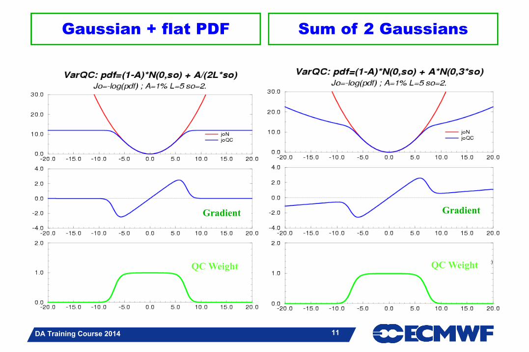
Gaussian + flat PDF
GradientGradient
QC WeightQC Weight
Sum of 2 Gaussians
11

DA Training Course 2014
Tuning the rejection limit
The left histogram on the left has been transformed into the right histogram such that the Gaussian part appears as a pair of straight lines forming a ‘V’ at zero.The slope of the lines gives the standard deviation of the Gaussian.
The rejection limit can be chosen to be where the actual distribution is some distance away from the ‘V’ - around 6 to 7 K in this case, would be appropriate.
12
DA Training Course 2014
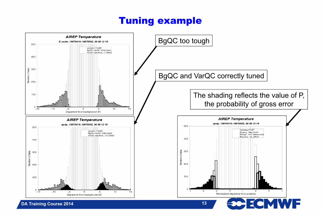
Tuning example
BgQC too tough
BgQC and VarQC correctly tuned
The shading reflects the value of P,the probability of gross error
13
DA Training Course 2014
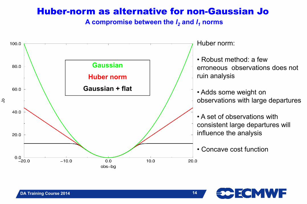
Huber-norm as alternative for non-Gaussian Jo A compromise between the l2 and l1 norms
Gaussian
Huber norm
Gaussian + flat
Huber norm:
• Robust method: a few erroneous observations does not ruin analysis
• Adds some weight on observations with large departures
• A set of observations with consistent large departures will influence the analysis
• Concave cost function
14
DA Training Course 2014
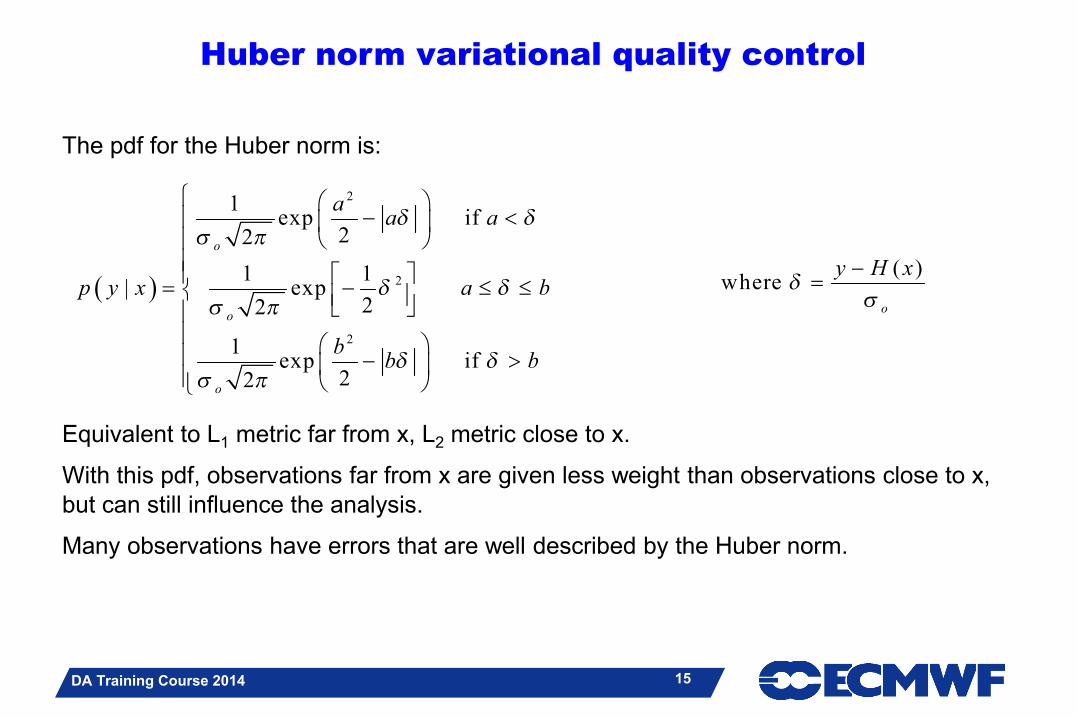
Huber norm variational quality control
The pdf for the Huber norm is:
Equivalent to L1 metric far from x, L2 metric close to x.
With this pdf, observations far from x are given less weight than observations close to x, but can still influence the analysis.
Many observations have errors that are well described by the Huber norm.
2
2
2
1exp if
22
1 1| exp
22
1exp if
22
o
o
o
aa a
p y x a b
bb b
( )where
o
y H x
15

DA Training Course 2014
Comparing observation weights:Huber-norm (red) versus Gaussian+flat (blue)
More weight in the middle of the distribution
More weight on the edges of the distribution
More influence of data with large departures
-Weights: 0 – 25%
25%
16
DA Training Course 2014
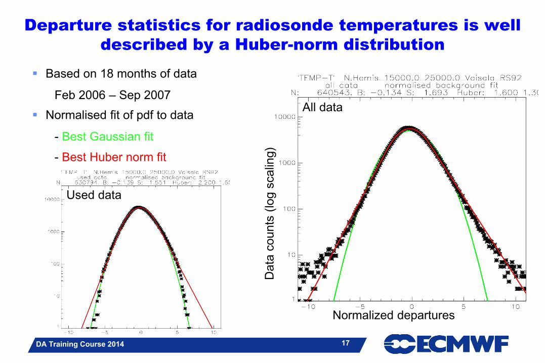
Departure statistics for radiosonde temperatures is well described by a Huber-norm distribution
Based on 18 months of data
Feb 2006 – Sep 2007
Normalised fit of pdf to data
- Best Gaussian fit
- Best Huber norm fit
Normalized departures
Data
counts
(lo
g s
calin
g)
All data
Used data
17
DA Training Course 2014
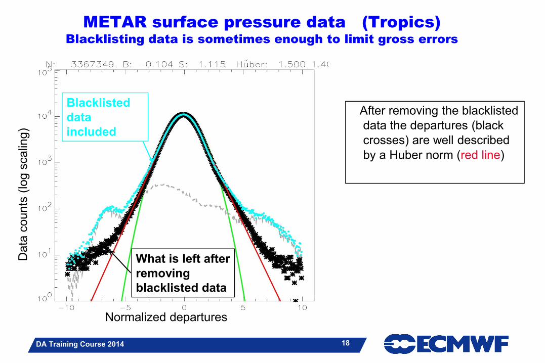
METAR surface pressure data (Tropics)Blacklisting data is sometimes enough to limit gross errors
Blacklisted data included
What is left after removing blacklisted data
After removing the blacklisted data the departures (black crosses) are well described by a Huber norm (red line)
Normalized departures
Data
counts
(lo
g s
calin
g)
18
DA Training Course 2014
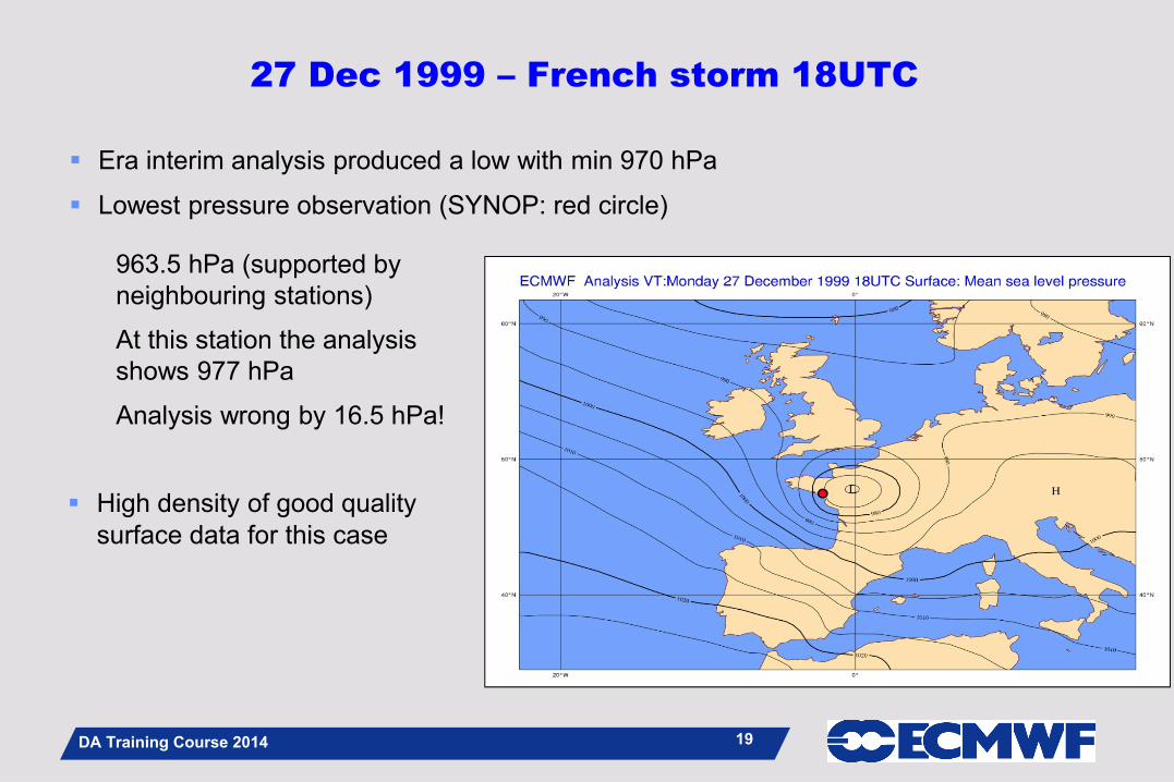
27 Dec 1999 – French storm 18UTC
963.5 hPa (supported by neighbouring stations)
At this station the analysis shows 977 hPa
Analysis wrong by 16.5 hPa!
High density of good quality surface data for this case
Era interim analysis produced a low with min 970 hPa
Lowest pressure observation (SYNOP: red circle)
19
DA Training Course 2014
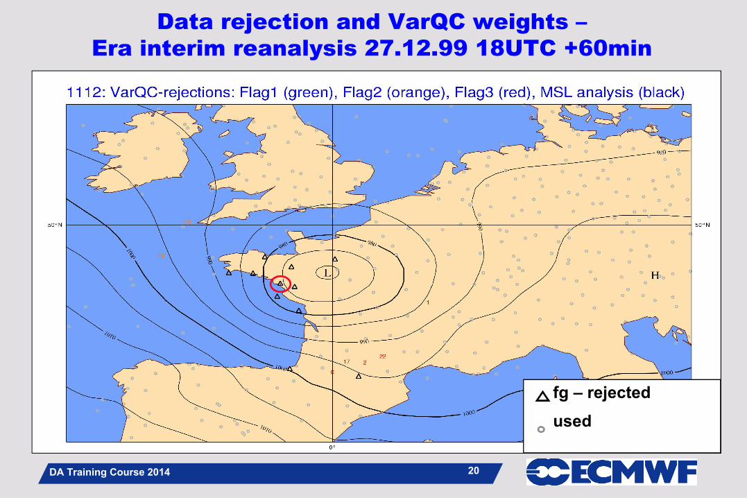
Data rejection and VarQC weights –Era interim reanalysis 27.12.99 18UTC +60min
fg – rejected
used
20
DA Training Course 2014
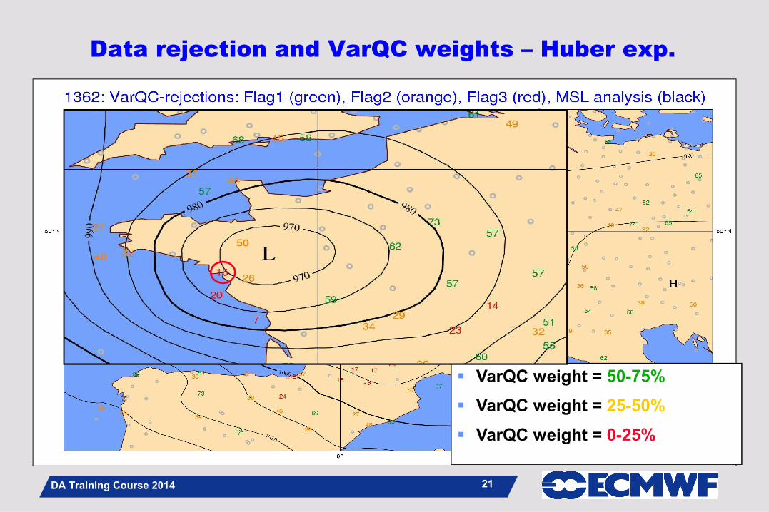
Data rejection and VarQC weights – Huber exp.
VarQC weight = 50-75%
VarQC weight = 25-50%
VarQC weight = 0-25%
21
DA Training Course 2014
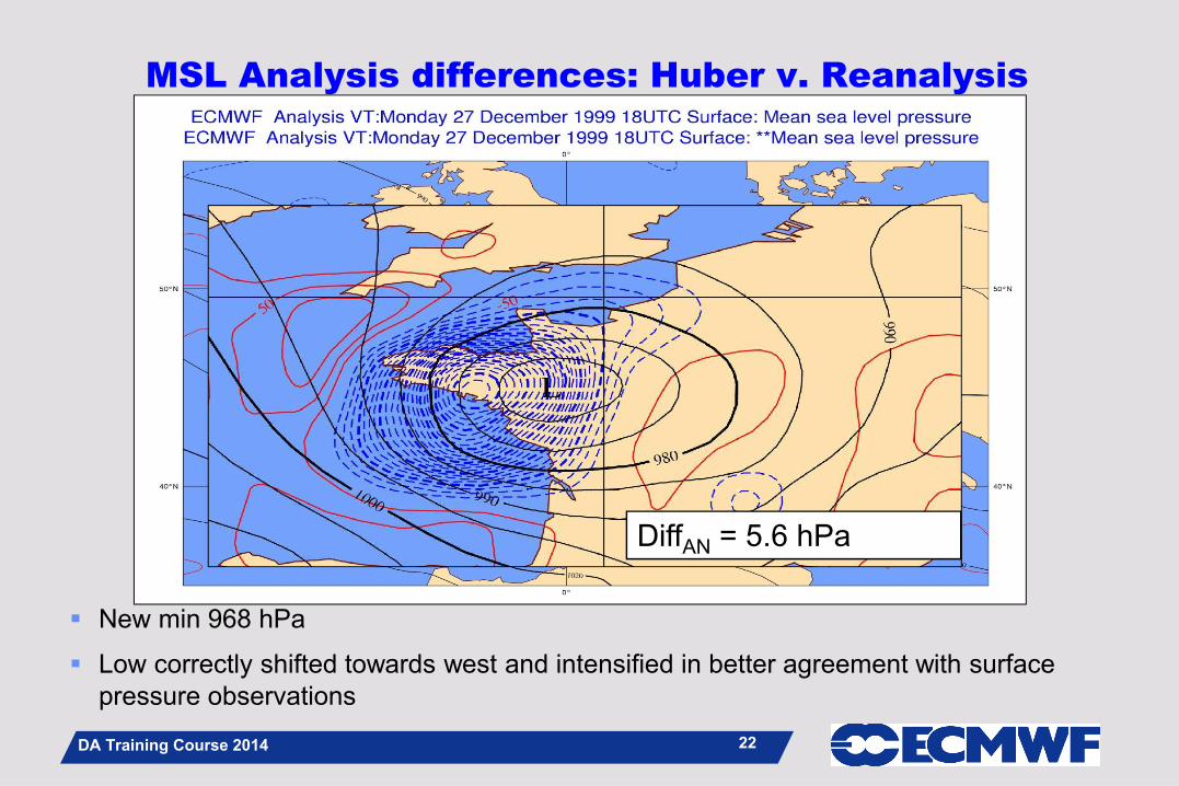
MSL Analysis differences: Huber v. Reanalysis
New min 968 hPa
Low correctly shifted towards west and intensified in better agreement with surface pressure observations
DiffAN = 5.6 hPa
22
DA Training Course 2014
VarQC general summary
VarQC provides a satisfactory and very efficient quality control mechanism - consistent with 3D/4D-Var.
The implementation can be very straight forward (multiply observation departures by a factor).
VarQC does not replace the pre-analysis checks - the checks against the background for example. However, with Huber-norm these are relaxed significantly.
All observational data from all data types are quality controlled simultaneously, as part of the general 3D/4D-Var minimisation.
A good description of background errors is essential foreffective, flow-dependent QC: background error lecture.
23