Embed Size (px)
DESCRIPTION
Huawei LTE Planning
Citation preview
Long Term Evolution (LTE) Radio Access Network Planning Guide
Long Term Evolution (LTE) Radio Access Network Planning Guide
1 How to Use This Guide ..............................................................................................................................1
1.1 Introduction ...............................................................................................................................................1
1.2 General Radio Network Planning Process ....................................................................................................1
1.3 Quick Guide to Content of Each Section .....................................................................................................2
2 LTE Fundamentals & Key Technologies .......................................................................................................3
2.1 Overview of Data Market as a Whole ..........................................................................................................3
2.2 3GPP Evolution and Market Expectation .....................................................................................................3
2.3 LTE Modulation Technology Highlight .........................................................................................................4
2.3.1 OFDM Fundamental .....................................................................................................................................................................5
2.3.2 SC-FDMA Fundamental ................................................................................................................................................................7
2.4 LTE Frame Structure ....................................................................................................................................8
2.5 LTE Resource Block Architecture ..................................................................................................................9
2.6 Reference Signal Structure ........................................................................................................................10
2.7 Timing and Sampling Architecture ............................................................................................................11
2.7.1 Normal and Extended Cyclic Prefix .............................................................................................................................................12
2.7.2 Synchronization Channel ............................................................................................................................................................13
2.8 Uplink Physical Channel Structure .............................................................................................................13
2.8.1 FDD Uplink Control, Sounding and Demodulation Reference Signal Structure ............................................................................14
2.9 Multiple Input Multiple Output (MIMO) ....................................................................................................15
2.9.1 3GPP MIMO Mode Definition .....................................................................................................................................................15
2.9.2 Open Loop MIMO ......................................................................................................................................................................16
2.9.3 Closed Loop MIMO ....................................................................................................................................................................17
2.9.4 Pre-coding Matrix ......................................................................................................................................................................18
2.9.5 Beam Forming ...........................................................................................................................................................................20
2.10 LTE FDD vs LTE TDD Main Features Comparison ......................................................................................21
2.11 LTE Channels Hierarchy Overview ............................................................................................................22
2.11.1 Physical Channel Modulation Schemes .....................................................................................................................................22
2.11.2 Downlink Channel Functionality Breakdown .............................................................................................................................23
2.11.3 Uplink Channel Functionality Breakdown .................................................................................................................................23
2.11.4 Channel Functionality Description in Detail ...............................................................................................................................23
2.11.5 Downlink Control Channel and RE Mapping Relationship .........................................................................................................25
2.12 Cell Search, Synchronization & Mobility–UE Call Flow View .....................................................................25
2.12.1 Cell Search and Synchronization ...............................................................................................................................................25
2.12.2 UE Procedure for Reporting Channel Quality Indication (CQI), Precoding Matrix indicator (PMI) and rank indication (RI) ...........26
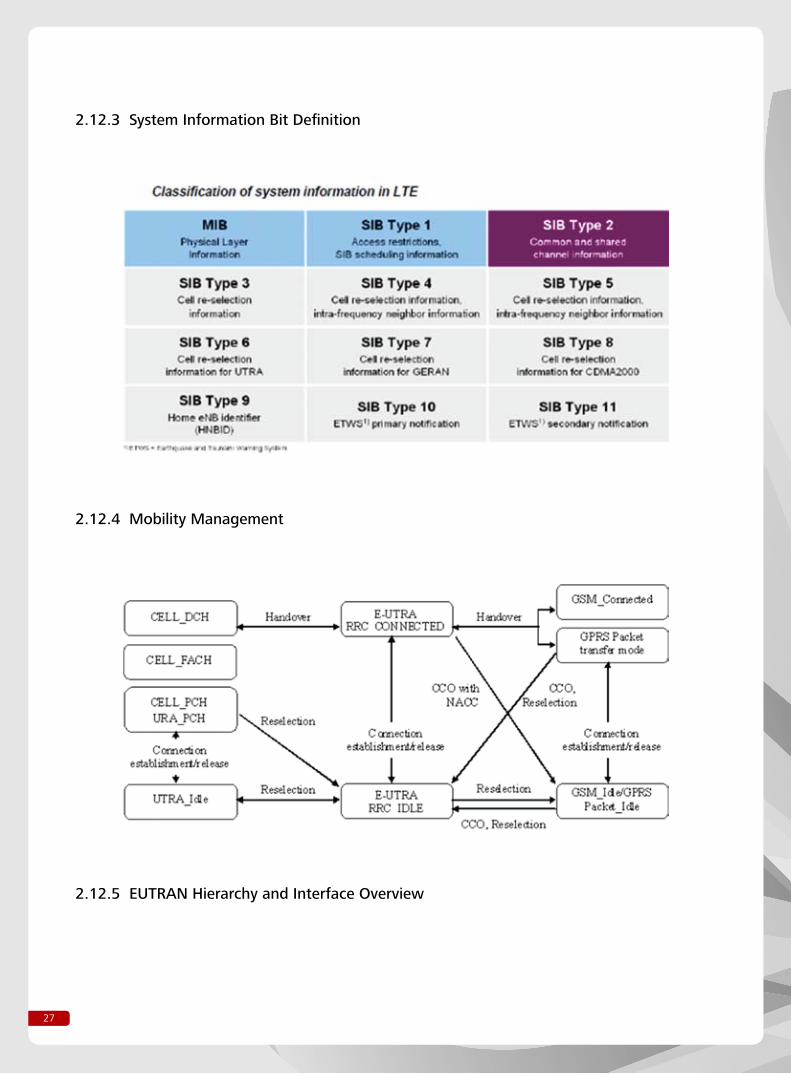
2.12.3 System Information Bit Definition .............................................................................................................................................27
2.12.4 Mobility Management ..............................................................................................................................................................27
2.12.5 EUTRAN Hierarchy and Interface Overview ...............................................................................................................................27
2.12.6 Summary of Handover Call Flow – 3GPP Example TS36.300 .....................................................................................................28
2.13 Example of Peak Data Rate Calculation ...................................................................................................29
3 LTE Frequency and Spectrum Planning .....................................................................................................30
3.1 Frequency Spectrum Overview - FDD ........................................................................................................30
3.2 Frequency Spectrum Overview - TDD ........................................................................................................30
3.3 Channel Bandwidth and Subcarrier Allocation ...........................................................................................31
3.4 Channel Arrangement ...............................................................................................................................32
3.4.1 Channel Spacing ........................................................................................................................................................................32
3.4.2 Channel Raster ...........................................................................................................................................................................32
3.4.3 Carrier Frequency and EARFCN ...................................................................................................................................................33
3.5 Frequency Planning Recommendations .....................................................................................................34
3.5.1 Conventional Frequency Reuse Scheme 1*3*1 ............................................................................................................................34
3.5.2 SFR 1*3*1 – Downlink and Uplink ..............................................................................................................................................35
3.5.3 TDD Specific Frequency Planning Considerations ........................................................................................................................36
3.5.4 Frequency Band Selection ..........................................................................................................................................................37
3.5.5 Cyclic Prefix Planning .................................................................................................................................................................38
3.5.6 Placing Multiple Technologies@Multiple Frequency Band ...........................................................................................................38
4 Link Budget and Coverage Planning .........................................................................................................40
4.1 Conventional Link Budget .........................................................................................................................41
4.2 Propagation Parameters ............................................................................................................................42
4.2.1 Channel Model ..........................................................................................................................................................................42
4.2.2 3GPP Value for Multipath and Doppler Effect .............................................................................................................................43
4.2.3 Propagation Model ....................................................................................................................................................................45
4.2.4 Penetration Loss .........................................................................................................................................................................50
4.2.5 Body Loss ...................................................................................................................................................................................51
4.2.6 Feeder Loss ................................................................................................................................................................................52
4.2.7 Background Noise ......................................................................................................................................................................53
4.3 Equipment-Related Parameters .................................................................................................................53
4.3.1 Transmit Power ..........................................................................................................................................................................53
4.3.2 Receiver Sensitivity .....................................................................................................................................................................54
4.3.3 Noise Figure ...............................................................................................................................................................................54
4.3.4 Antenna Gain .............................................................................................................................................................................54
4.4 LTE-Related Parameters .............................................................................................................................56
4.4.1 MIMO Gains ..............................................................................................................................................................................56
4.4.2 Cell Edge Rate ............................................................................................................................................................................57
4.4.3 Interference Margin ...................................................................................................................................................................59
4.4.4 Beam Forming ...........................................................................................................................................................................59
4.5 System Reliability ......................................................................................................................................60
4.5.1 Slow Fading Margin ...................................................................................................................................................................60
4.5.2 Effect of Earth Curvature ............................................................................................................................................................62
4.5.3 Absence of Fast Fading and Soft Handover Margin ....................................................................................................................62
4.6 Specific Factors in Link Budget Consideration ............................................................................................62
4.6.1 Features Overview ......................................................................................................................................................................62
4.6.2 TTI Bundling ...............................................................................................................................................................................63
4.6.3 Interference Rejection Combining ..............................................................................................................................................63
4.6.4 Reference Signal Power Boosting Gain .......................................................................................................................................65
4.6.5 Remote Radio Unit and eNodeB Portfolio ...................................................................................................................................65
4.7 Summary of Variables inside Link Budget Tools .........................................................................................65
5 Interference and Guard Band Analysis ......................................................................................................69
5.1 Overview ..................................................................................................................................................69
5.1.1 Basic Concepts ...........................................................................................................................................................................69
5.1.2 Analysis of Background Noise ....................................................................................................................................................73
5.1.3 Impact of Interference ...............................................................................................................................................................74
5.2 Interference Between TDD Systems ...........................................................................................................75
5.2.1 Interference between Different Carriers ......................................................................................................................................75
5.2.2 Interference within the Same Carrier ..........................................................................................................................................76
5.2.3 Theoretical Analysis of Interference under Site Sharing ...............................................................................................................77
5.2.4 Theoretical Analysis of Interference: Non Colocated eNodeB .....................................................................................................78
5.3 Guard Band Requirement: LTE-FDD vs GSM/UMTS ....................................................................................79
5.4 GuardBand Requirement: LTE FDD vs LTE TDD ..........................................................................................79
5.5 Spectrum Refarming for LTE ......................................................................................................................80
5.5.1 Summary ...................................................................................................................................................................................80
5.5.2 GSM Spectrum Refarming ..........................................................................................................................................................80
5.5.3 Introduction of Buffer Zone ........................................................................................................................................................81
5.6 Radio Access Technologies Co-location Strategies .....................................................................................82
5.6.1 Overview ...................................................................................................................................................................................82
5.6.2 GSM-LTE Co-Location Examples .................................................................................................................................................82
5.6.3 LTE TDD and WiMAX Systems Co-Location .................................................................................................................................87
6 LTE Access Network Capacity Planning .....................................................................................................89
6.1 Definition of Capacity ...............................................................................................................................89
6.2 3GPP Services Classification ......................................................................................................................91
6.3 EUTRAN Capacity Limiting Factors ............................................................................................................91
6.3.1 Operating Frequency Band .........................................................................................................................................................92
6.3.2 RF coverage - RSRP ....................................................................................................................................................................93
6.3.3 Impact of Interference on Capacity ............................................................................................................................................93
6.3.4 Signal Interference Noise Ratio and Adaptive Coding .................................................................................................................94
6.3.5 Radio (Transmitter) Power Availability .........................................................................................................................................94
6.3.6 Spectrum Bandwidth Availability ................................................................................................................................................94
6.3.7 Base Band Channel Card Processing Capacity .............................................................................................................................94
6.3.8 S1/X2 Capacity ...........................................................................................................................................................................94
6.3.9 Application of Special Antenna Technologies (MIMO/BF/V MIMO) ..............................................................................................94
6.3.10 Scheduling Mode .....................................................................................................................................................................95
6.3.11 Actual Cell Site Placement in Relation to Traffic ........................................................................................................................96
6.3.12 UE Capability ............................................................................................................................................................................96
6.3.13 User Traffic Mix and Call Modelling ..........................................................................................................................................97
6.3.14 Time Slot Allocation for Uplink and Downlink – TDD specific ....................................................................................................97
6.3.15 Cyclical Prefix Allocation ...........................................................................................................................................................98
6.4 S1 Bandwidth Dimensioning Procedure .....................................................................................................98
6.5 X2 Bandwidth Dimensioning Procedure ....................................................................................................99
6.6 Impact of Latency of X2 on Cell Throughput ...........................................................................................100
6.7 Inter Radio Access Technology Handover Considerations ........................................................................100
7 U-Net Simulation and Operation ............................................................................................................103
7.1 Introduction ............................................................................................................................................103
7.2 Simulation Process ..................................................................................................................................103
7.3 Creating Project ......................................................................................................................................104
7.4 Geographical Information .......................................................................................................................104
7.4.1 Quick Import Function .............................................................................................................................................................104
7.4.2 Defining Coordinate Systems ....................................................................................................................................................105
7.4.3 Properties of Clutter Class ........................................................................................................................................................106
7.5 Equipment Parameter .............................................................................................................................107
7.5.1 Overview .................................................................................................................................................................................107
7.5.2 Network Settings .....................................................................................................................................................................107
7.5.3 Equipment ...............................................................................................................................................................................113
7.5.4 Site, Cell and Transmitter Listing ..............................................................................................................................................113
7.5.5 Viewing “Hidden” Parameters ..................................................................................................................................................115
7.5.6 Propagation Model Selection ...................................................................................................................................................115
7.5.7 Clutter Related Modelling ........................................................................................................................................................118
7.5.8 Impact of Parameter Setting on Prediction and Simulation .......................................................................................................118
7.6 Engineering Parameter ............................................................................................................................119
7.6.1 Power Setting ..........................................................................................................................................................................119
7.6.2 Load Setting ............................................................................................................................................................................121
7.6.3 Frequency Planning ..................................................................................................................................................................122
7.6.4 Scheduling Parameters .............................................................................................................................................................125
7.6.5 Antenna Property .....................................................................................................................................................................126
7.6.6 Properties of a Single Transmitter .............................................................................................................................................128
7.6.7 Properties of a eNodeB Template .............................................................................................................................................130
7.7 LTE Traffic Model Parameters ..................................................................................................................132
7.7.1 Overview .................................................................................................................................................................................132
7.7.2 Environments ...........................................................................................................................................................................132
7.7.3 User Profiles .............................................................................................................................................................................133
7.7.4 Terminals .................................................................................................................................................................................134
7.7.5 Mobility Types ..........................................................................................................................................................................135
7.7.6 Services ....................................................................................................................................................................................136
7.7.7 Traffic Map ..............................................................................................................................................................................137
7.8 Prediction and Simulation .......................................................................................................................141
7.8.1 Predictions ...............................................................................................................................................................................141
7.8.2 Simulation ................................................................................................................................................................................145
7.9 Point Analysis Tool ..................................................................................................................................151
7.9.1 Profile ......................................................................................................................................................................................151
7.9.2 Reception ................................................................................................................................................................................151
7.9.3 Signal Analysis .........................................................................................................................................................................152
7.9.4 Result ......................................................................................................................................................................................152
7.10 RF Cell Planning Optimization ...............................................................................................................152
7.11 U-Net Planning Case .............................................................................................................................154
7.11.1 Overview of Planning Area .....................................................................................................................................................154
7.11.2 Site Distribution .....................................................................................................................................................................155
7.11.3 Parameter Configuration and General Assumption .................................................................................................................156
7.11.4 Network Coverage Predictions ...............................................................................................................................................157
7.11.5 Network Capacity Simulation .................................................................................................................................................160
8 LTE Network Key Performance Indicators ...............................................................................................163
8.1 KPI Measurement Methodology ..............................................................................................................163
8.2 KPI Acceptance Procedure ......................................................................................................................163
8.3 Service KPIs and Network KPIs ................................................................................................................164
8.4 Cluster and Test Route ............................................................................................................................164
8.5 Proposed Key Performance Indicators .....................................................................................................165
8.6 Proposed KPIs for Final Acceptance (Stability Acceptance, Optional) .......................................................165
9 Network Planning Checklist ...................................................................................................................166
9.1 Introduction ............................................................................................................................................166
9.2 Checklist Items Consideration .................................................................................................................166
9.2.1 Understanding Customer Spectrum Bandwidth Availability .......................................................................................................166
9.2.2 Actual Frequency Band Allocation for LTE .................................................................................................................................166
9.2.3 Frequency Band Refarming Requirement for LTE ......................................................................................................................167
9.2.4 Location of Customer Coverage Requirement ...........................................................................................................................167
9.2.5 Highway and Tunnel Coverage Requirement ............................................................................................................................168
9.2.6 Evaluate Existing Network Condition for InterRAT ....................................................................................................................168
9.2.7 Terrain and Clutter Database Availability and Accuracy .............................................................................................................168
9.2.8 Scheduler Selection ..................................................................................................................................................................169
9.2.9 Indoor Coverage Requirement .................................................................................................................................................169
9.2.10 Cell Edge Throughput Requirement ........................................................................................................................................169
9.2.11 Call Model and SmartPhone Penetration Growth Considerations ............................................................................................169
9.2.12 Base Station Antenna and Other Co-siting Equipment Selection .............................................................................................170
9.2.13 Interference Protection and Isolation Requirement .................................................................................................................170
9.2.14 Radio Related Equipment Selection ........................................................................................................................................171
9.2.15 Network and Spectrum Evolution Consideration ....................................................................................................................171
9.2.16 MIMO and Beam Forming Implementation ............................................................................................................................171
9.2.17 Cyclic Prefix Planning .............................................................................................................................................................171
9.2.18 Understanding of Current Transmission Backhaul Network Capability .....................................................................................172
9.2.19 UE Distribution and Channel Model : Pedestrian vs High Mobility ...........................................................................................172
9.2.20 TDD Specific Uplink and Downlink Configuration ...................................................................................................................172
9.2.21 Power Boosting Configuration ...............................................................................................................................................172
10 Appendix: RF Antenna Systems ..............................................................................................................174
10.1 Overview ..............................................................................................................................................174
10.2 Antenna Classification ..........................................................................................................................174
10.2.1 Frequency ..............................................................................................................................................................................174
10.2.2 Directivity ...............................................................................................................................................................................174
10.3 Main Specifications of Antenna ............................................................................................................174
10.3.1 Work Band .............................................................................................................................................................................175
10.3.2 Antenna Gain .........................................................................................................................................................................175
10.3.3 Antenna Pattern .....................................................................................................................................................................176
10.3.4 Beamwidth ............................................................................................................................................................................177
10.3.5 Relation between Beamwidth and Gain .................................................................................................................................177
10.3.6 Front-to-rear Ratio .................................................................................................................................................................178
10.3.7 Upper Side Lobe Suppression .................................................................................................................................................178
10.3.8 Polarization Mode ..................................................................................................................................................................179
10.3.9 Down Tilt ...............................................................................................................................................................................179
10.3.10 VSWR (Voltage Standing Wave Ratio) ...................................................................................................................................179
10.3.11 Port Isolation .......................................................................................................................................................................180
10.3.12 Power Capacity ....................................................................................................................................................................180
10.3.13 Input Port of Antenna ..........................................................................................................................................................180
10.3.14 Passive Intermodulation (PIM) ..............................................................................................................................................180
10.3.15 Dimensions and Weight of Antenna .....................................................................................................................................181
10.3.16 Wind Load ...........................................................................................................................................................................181
10.3.17 Work Temperature and Humidity .........................................................................................................................................181
10.3.18 Lightning Protection .............................................................................................................................................................181
10.3.19 Three-proof Capability ..........................................................................................................................................................181
10.3.20 Camouflaged Antenna Scheme for Sites ...............................................................................................................................181
10.3.21 Customized Camouflage ......................................................................................................................................................182
10.3.22 Outlook Camouflage ............................................................................................................................................................183
10.3.23 Antenna Camouflage in Special Environment .......................................................................................................................183
11 References ...........................................................................................................................................184
1
1.1 Introduction
The purpose of this document is to provide systems engineers/planners with a set of guidelines and introductions to
LTE deployment planning that may aid the design of a high quality Long Term Evolution (LTE) RF System. In general,
most of the content provided in this planning guide can be applied to LTE system design with field implementation
considerations. Specific RF planning information unique to Huawei’s LTE EUTRAN product is also provided.
Although there are numerous and detailed references made to particular tools, it is not the purpose of this planning
document to replace any product and tools' operating manual/instruction. Please refer to the official publications of
the respective product/tool for their most up to date functionality.
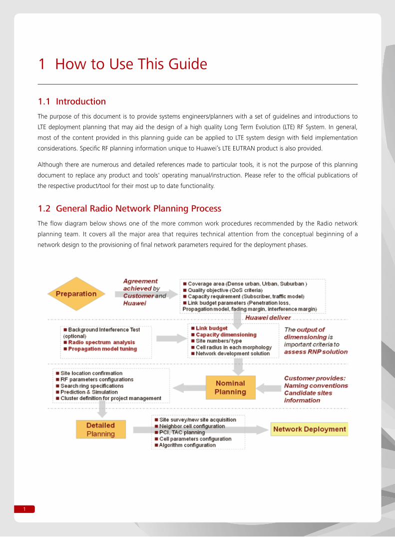
1.2 General Radio Network Planning Process
The flow diagram below shows one of the more common work procedures recommended by the Radio network
planning team. It covers all the major area that requires technical attention from the conceptual beginning of a
network design to the provisioning of final network parameters required for the deployment phases.
1 How to Use This Guide
2
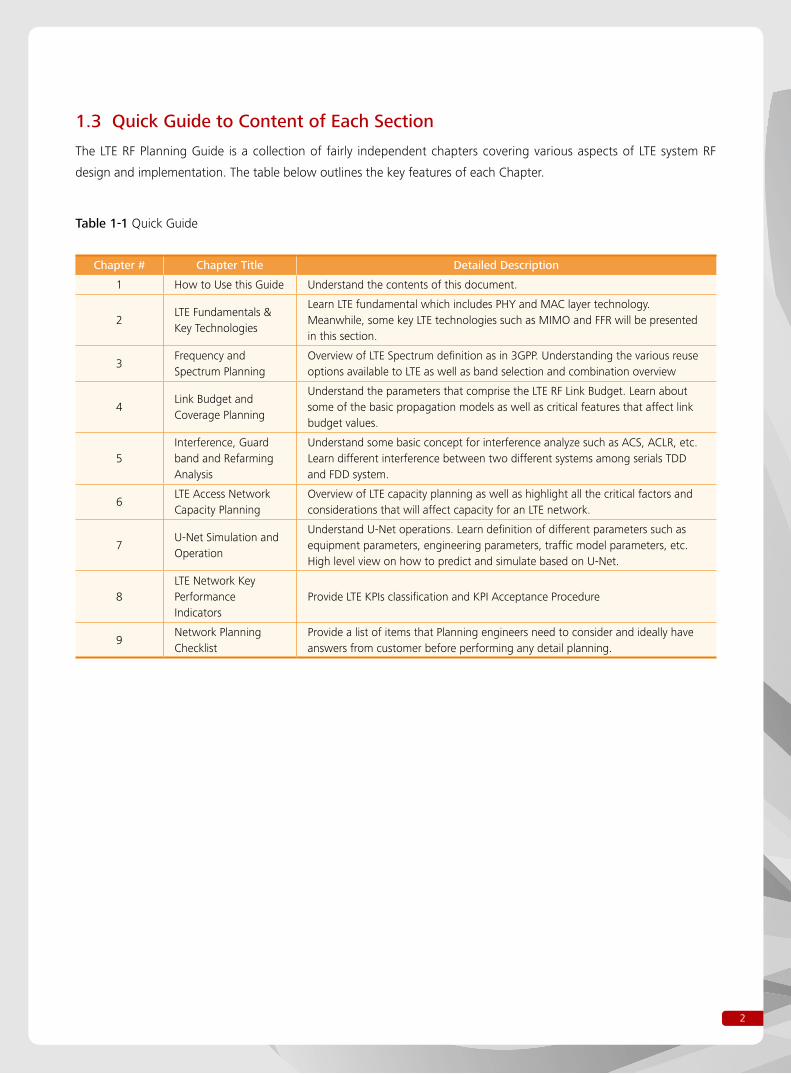
1.3 Quick Guide to Content of Each Section
The LTE RF Planning Guide is a collection of fairly independent chapters covering various aspects of LTE system RF
design and implementation. The table below outlines the key features of each Chapter.
Chapter # Chapter Title Detailed Description
1 How to Use this Guide Understand the contents of this document.
2LTE Fundamentals & Key Technologies
Learn LTE fundamental which includes PHY and MAC layer technology. Meanwhile, some key LTE technologies such as MIMO and FFR will be presented in this section.
3Frequency and Spectrum Planning
Overview of LTE Spectrum definition as in 3GPP. Understanding the various reuse options available to LTE as well as band selection and combination overview
4Link Budget and Coverage Planning
Understand the parameters that comprise the LTE RF Link Budget. Learn about some of the basic propagation models as well as critical features that affect link budget values.
5Interference, Guard band and Refarming Analysis
Understand some basic concept for interference analyze such as ACS, ACLR, etc. Learn different interference between two different systems among serials TDD and FDD system.
6LTE Access Network Capacity Planning
Overview of LTE capacity planning as well as highlight all the critical factors and considerations that will affect capacity for an LTE network.
7U-Net Simulation and Operation
Understand U-Net operations. Learn definition of different parameters such as equipment parameters, engineering parameters, traffic model parameters, etc. High level view on how to predict and simulate based on U-Net.
8LTE Network Key Performance Indicators
Provide LTE KPIs classification and KPI Acceptance Procedure
9Network Planning Checklist
Provide a list of items that Planning engineers need to consider and ideally have answers from customer before performing any detail planning.
Table 1-1 Quick Guide
3
2 LTE Fundamentals & Key Technologies
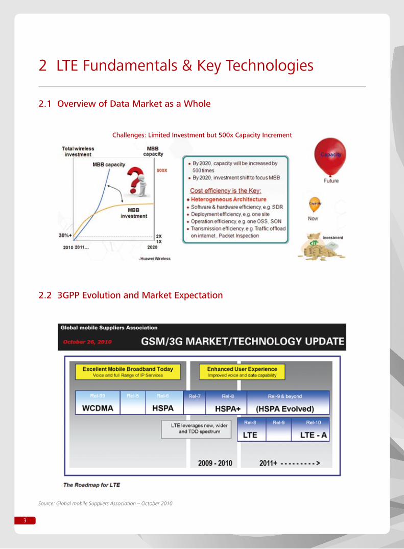
2.1 Overview of Data Market as a Whole
Challenges: Limited Investment but 500x Capacity Increment
2.2 3GPP Evolution and Market Expectation
Source: Global mobile Suppliers Association – October 2010
4
2.3 LTE Modulation Technology Highlight
In Nov. 2004, 3GPP began a project to define the long-term evolution (LTE) of Universal Mobile Telecommunications
System (UMTS) cellular technology. The main goal is to provide
Higher throughput performance •
100 Mbit/s peak downlink, 50 Mbit/s peak uplink•
1G for LTE Advanced•
Higher cell edge performance•
Reduced latency in setup time. Shorter transfer delay, shorter handover latency and interruption time for better •
user experience
Support of variable and scalable bandwidth (1.4, 3, 5, 10, 15 and 20 MHz)•
Backwards compatible with Existing 3G technologies •
Works with GSM/EDGE/UMTS systems•
Utilizes existing 2G and 3G spectrum and new spectrum•
Supports hand-over and roaming to existing mobile networks•
Quality of Service Support. •
Wide application •
TDD (unpaired) and FDD (paired) spectrum modes•
Mobility up to 450km/h•
Large range of terminals (phones and PCs to cameras)•
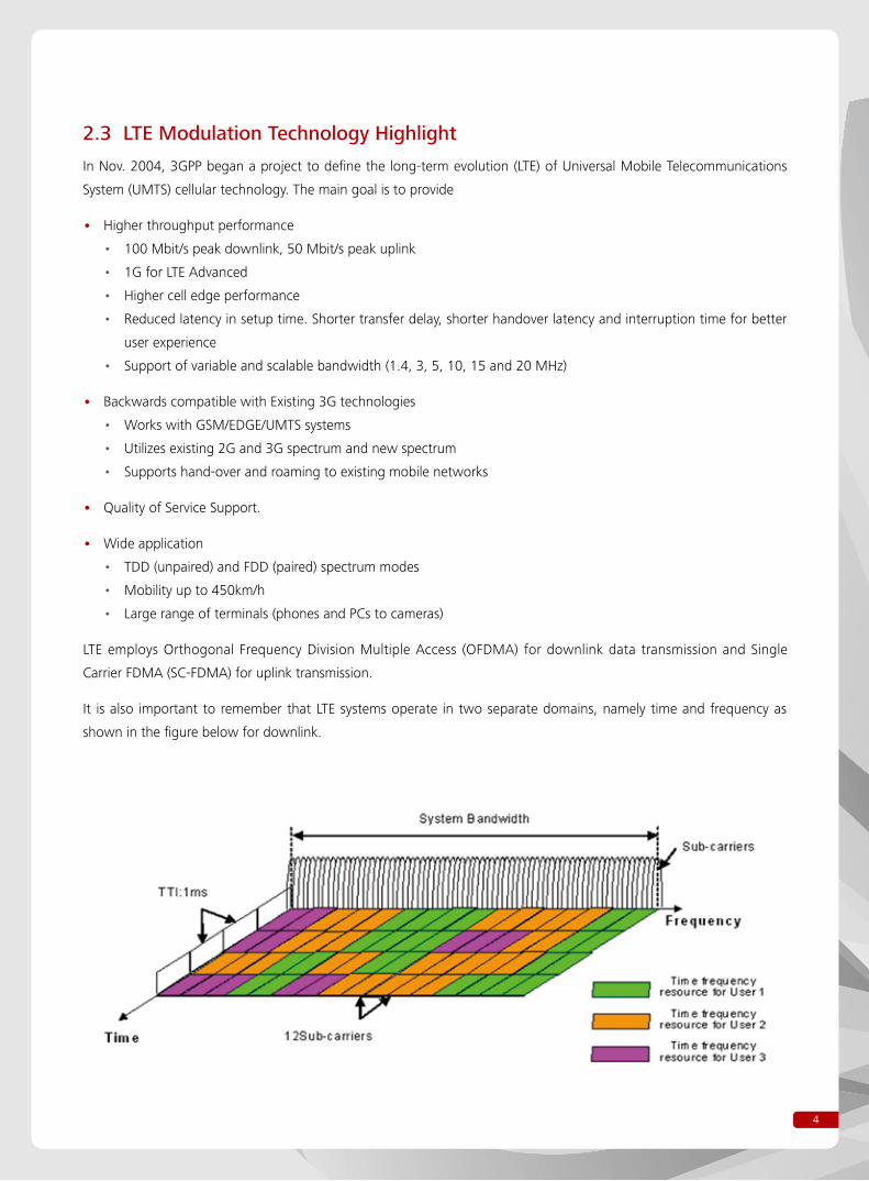
LTE employs Orthogonal Frequency Division Multiple Access (OFDMA) for downlink data transmission and Single
Carrier FDMA (SC-FDMA) for uplink transmission.
It is also important to remember that LTE systems operate in two separate domains, namely time and frequency as
shown in the figure below for downlink.
5
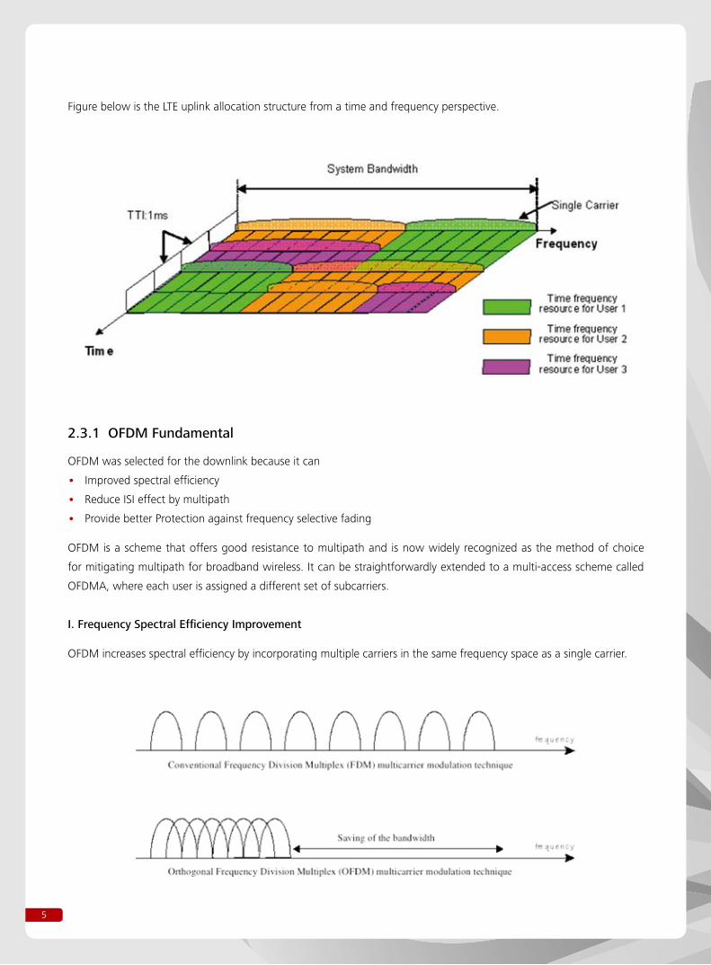
Figure below is the LTE uplink allocation structure from a time and frequency perspective.
2.3.1 OFDM Fundamental
OFDM was selected for the downlink because it can
Improved spectral efficiency •
Reduce ISI effect by multipath •
Provide better Protection against frequency selective fading •
OFDM is a scheme that offers good resistance to multipath and is now widely recognized as the method of choice
for mitigating multipath for broadband wireless. It can be straightforwardly extended to a multi-access scheme called
OFDMA, where each user is assigned a different set of subcarriers.
I. Frequency Spectral Efficiency Improvement
OFDM increases spectral efficiency by incorporating multiple carriers in the same frequency space as a single carrier.
6
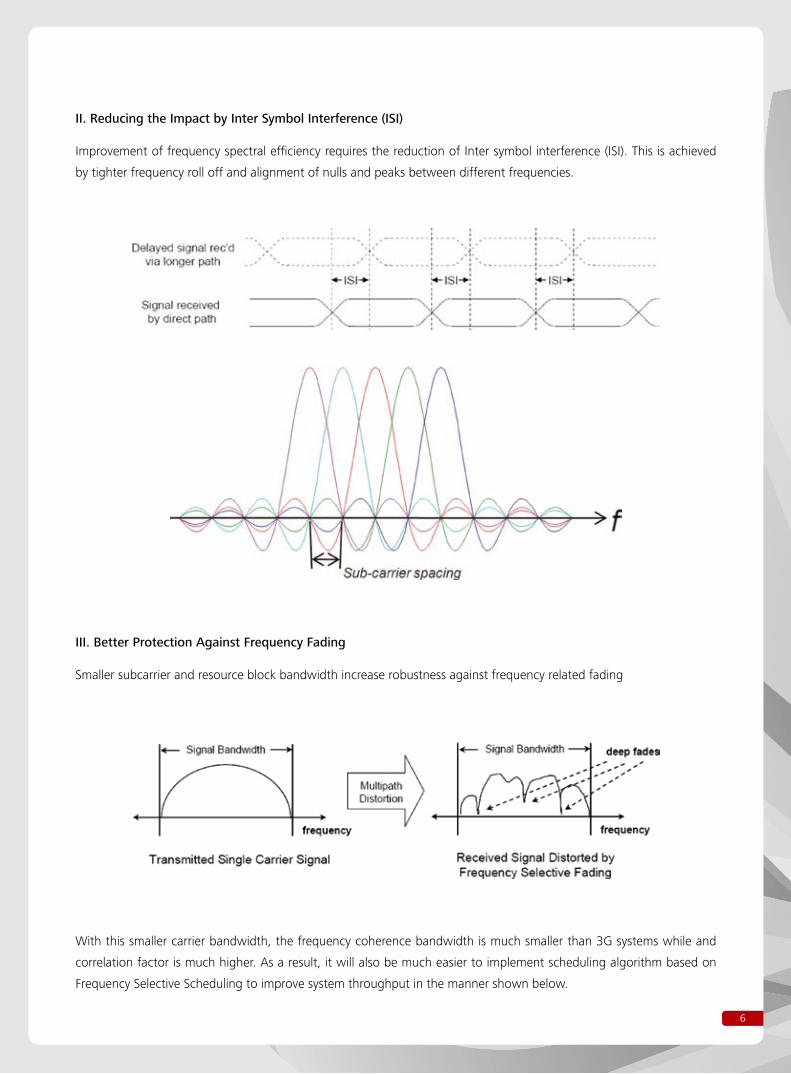
II. Reducing the Impact by Inter Symbol Interference (ISI)
Improvement of frequency spectral efficiency requires the reduction of Inter symbol interference (ISI). This is achieved
by tighter frequency roll off and alignment of nulls and peaks between different frequencies.
III. Better Protection Against Frequency Fading
Smaller subcarrier and resource block bandwidth increase robustness against frequency related fading
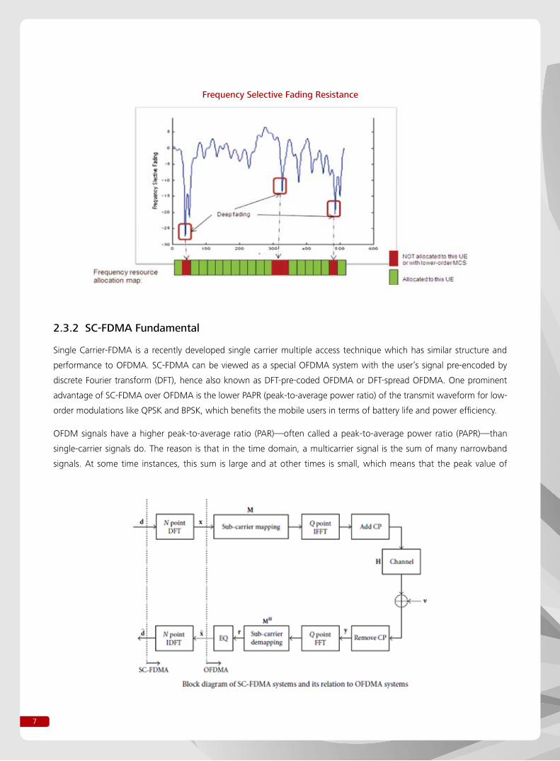
With this smaller carrier bandwidth, the frequency coherence bandwidth is much smaller than 3G systems while and
correlation factor is much higher. As a result, it will also be much easier to implement scheduling algorithm based on
Frequency Selective Scheduling to improve system throughput in the manner shown below.
7
2.3.2 SC-FDMA Fundamental
Single Carrier-FDMA is a recently developed single carrier multiple access technique which has similar structure and
performance to OFDMA. SC-FDMA can be viewed as a special OFDMA system with the user’s signal pre-encoded by
discrete Fourier transform (DFT), hence also known as DFT-pre-coded OFDMA or DFT-spread OFDMA. One prominent
advantage of SC-FDMA over OFDMA is the lower PAPR (peak-to-average power ratio) of the transmit waveform for low-
order modulations like QPSK and BPSK, which benefits the mobile users in terms of battery life and power efficiency.
OFDM signals have a higher peak-to-average ratio (PAR)—often called a peak-to-average power ratio (PAPR)—than
single-carrier signals do. The reason is that in the time domain, a multicarrier signal is the sum of many narrowband
signals. At some time instances, this sum is large and at other times is small, which means that the peak value of
Frequency Selective Fading Resistance
8
the signal is substantially larger than the average value. This high PAR is one of the most important implementation
challenges that face OFDM, because it reduces the efficiency and hence increases the cost of the RF power amplifier,
which is one of the most expensive components in the radio. The figure below shows the relationship between OFDM
and SC-FDMA in LTE.
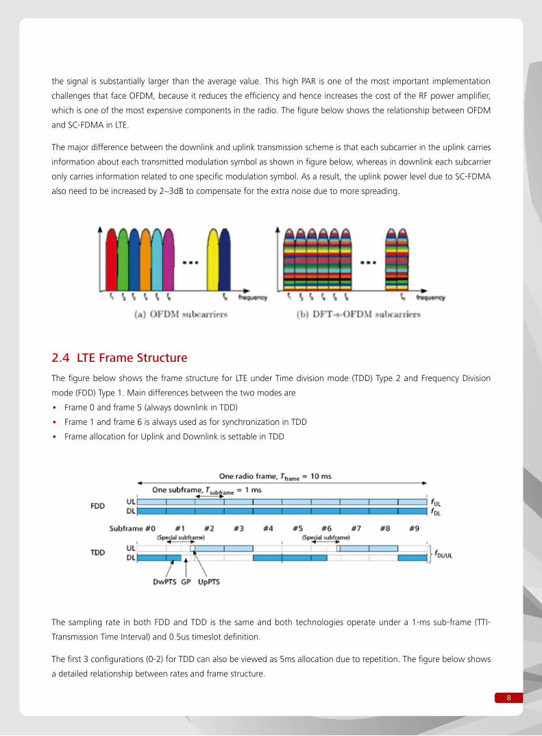
The major difference between the downlink and uplink transmission scheme is that each subcarrier in the uplink carries
information about each transmitted modulation symbol as shown in figure below, whereas in downlink each subcarrier
only carries information related to one specific modulation symbol. As a result, the uplink power level due to SC-FDMA
also need to be increased by 2~3dB to compensate for the extra noise due to more spreading.
2.4 LTE Frame Structure
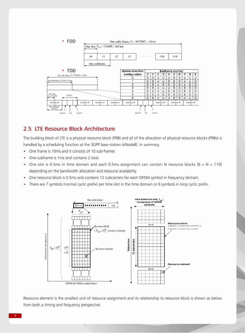
The figure below shows the frame structure for LTE under Time division mode (TDD) Type 2 and Frequency Division
mode (FDD) Type 1. Main differences between the two modes are
Frame 0 and frame 5 (always downlink in TDD) •
Frame 1 and frame 6 is always used as for synchronization in TDD •
Frame allocation for Uplink and Downlink is settable in TDD •
The sampling rate in both FDD and TDD is the same and both technologies operate under a 1-ms sub-frame (TTI-
Transmission Time Interval) and 0.5us timeslot definition.
The first 3 configurations (0-2) for TDD can also be viewed as 5ms allocation due to repetition. The figure below shows
a detailed relationship between rates and frame structure.
9
2.5 LTE Resource Block Architecture
The building block of LTE is a physical resource block (PRB) and all of the allocation of physical resource blocks (PRBs) is
handled by a scheduling function at the 3GPP base station (eNodeB). In summary,
One frame is 10ms and it consists of 10 sub-frames •
One subframe is 1ms and contains 2 slots •
One slot is 0.5ms in time domain and each 0.5ms assignment can contain N resource blocks [6 < N < 110] •
depending on the bandwidth allocation and resource availability.
One resource block is 0.5ms and contains 12 subcarriers for each OFDM symbol in frequency domain. •
There are 7 symbols (normal cyclic prefix) per time slot in the time domain or 6 symbols in long cyclic prefix. •
Resource element is the smallest unit of resource assignment and its relationship to resource block is shown as below
from both a timing and frequency perspective.
10
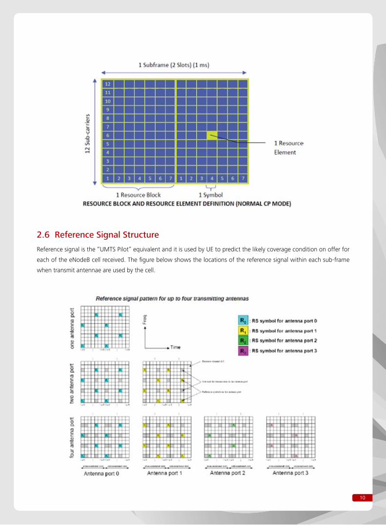
2.6 Reference Signal Structure
Reference signal is the “UMTS Pilot” equivalent and it is used by UE to predict the likely coverage condition on offer for
each of the eNodeB cell received. The figure below shows the locations of the reference signal within each sub-frame
when transmit antennae are used by the cell.
11
As LTE is a MIMO based technology, it can have more than two transmit antennae and in order to avoid reference
signals from the same cell interfering with each other, different antennae will be transmitting reference signal at
different time and frequency and how these are allocated are shown below.
As defined in the standard for TDD operations, the channel-sounding mechanism involves the UE’s transmitting a
deterministic signal that can be used by the eNodeB to estimate the UL channel from the UE. If the UL and DL channels are
properly calibrated, the eNodeB can then use the UL channel as an estimate of the DL channel, due to channel reciprocity.
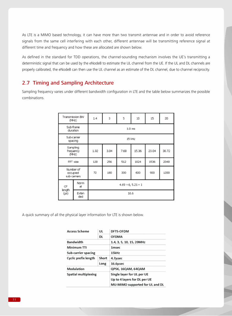
2.7 Timing and Sampling Architecture
Sampling frequency varies under different bandwidth configuration in LTE and the table below summarizes the possible
combinations.
A quick summary of all the physical layer information for LTE is shown below.
12
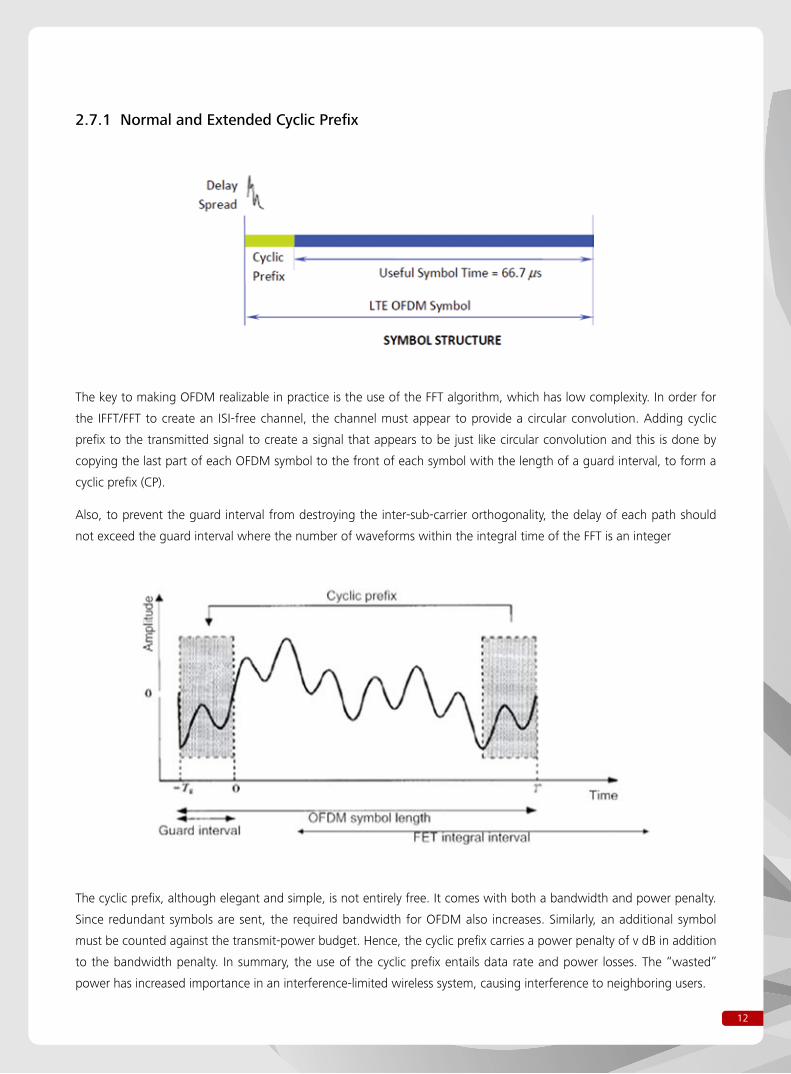
2.7.1 Normal and Extended Cyclic Prefix
The key to making OFDM realizable in practice is the use of the FFT algorithm, which has low complexity. In order for
the IFFT/FFT to create an ISI-free channel, the channel must appear to provide a circular convolution. Adding cyclic
prefix to the transmitted signal to create a signal that appears to be just like circular convolution and this is done by
copying the last part of each OFDM symbol to the front of each symbol with the length of a guard interval, to form a
cyclic prefix (CP).
Also, to prevent the guard interval from destroying the inter-sub-carrier orthogonality, the delay of each path should
not exceed the guard interval where the number of waveforms within the integral time of the FFT is an integer
The cyclic prefix, although elegant and simple, is not entirely free. It comes with both a bandwidth and power penalty.
Since redundant symbols are sent, the required bandwidth for OFDM also increases. Similarly, an additional symbol
must be counted against the transmit-power budget. Hence, the cyclic prefix carries a power penalty of v dB in addition
to the bandwidth penalty. In summary, the use of the cyclic prefix entails data rate and power losses. The “wasted”
power has increased importance in an interference-limited wireless system, causing interference to neighboring users.
13
Where L is the power used for non CP transmission. In the case where there is a large delay spread, e.g. due to large
cell radius, an extended CP option can be used.
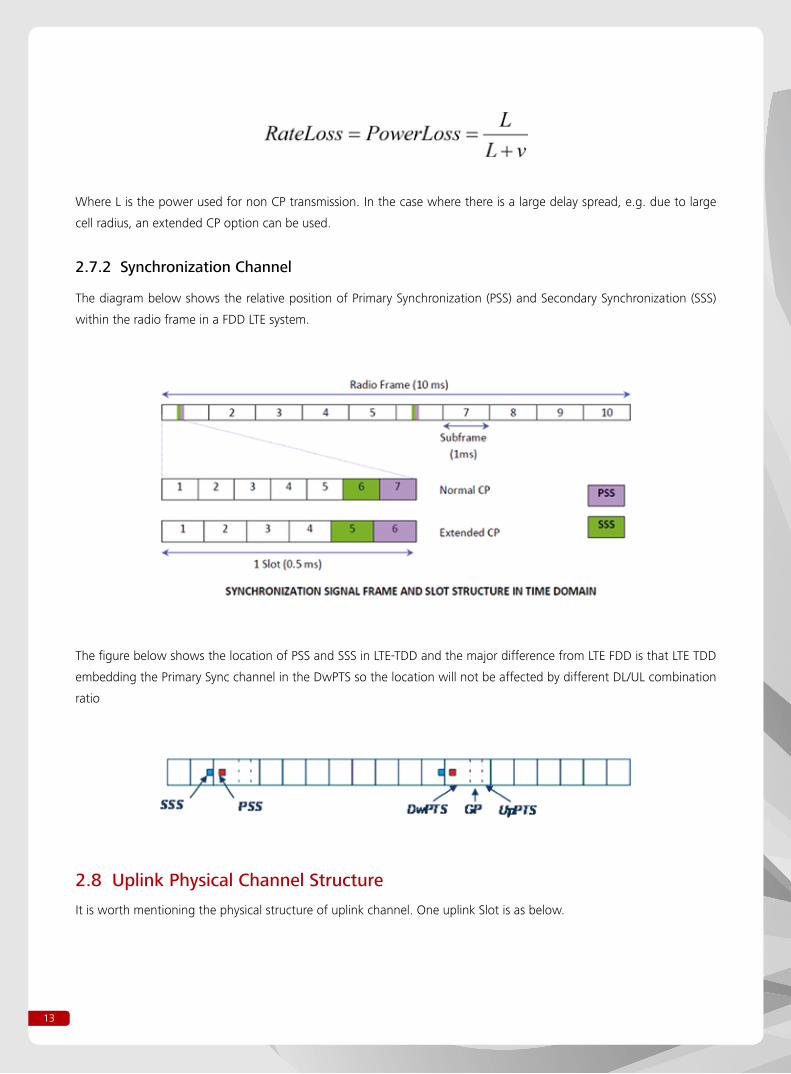
2.7.2 Synchronization Channel
The diagram below shows the relative position of Primary Synchronization (PSS) and Secondary Synchronization (SSS)
within the radio frame in a FDD LTE system.
The figure below shows the location of PSS and SSS in LTE-TDD and the major difference from LTE FDD is that LTE TDD
embedding the Primary Sync channel in the DwPTS so the location will not be affected by different DL/UL combination
ratio
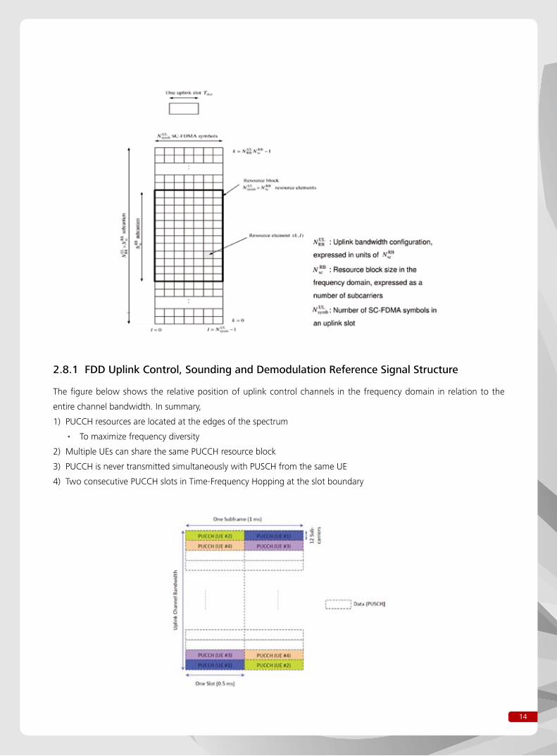
2.8 Uplink Physical Channel Structure
It is worth mentioning the physical structure of uplink channel. One uplink Slot is as below.
14
2.8.1 FDD Uplink Control, Sounding and Demodulation Reference Signal Structure
The figure below shows the relative position of uplink control channels in the frequency domain in relation to the
entire channel bandwidth. In summary,
1) PUCCH resources are located at the edges of the spectrum
To maximize frequency diversity•
2) Multiple UEs can share the same PUCCH resource block
3) PUCCH is never transmitted simultaneously with PUSCH from the same UE
4) Two consecutive PUCCH slots in Time-Frequency Hopping at the slot boundary
15
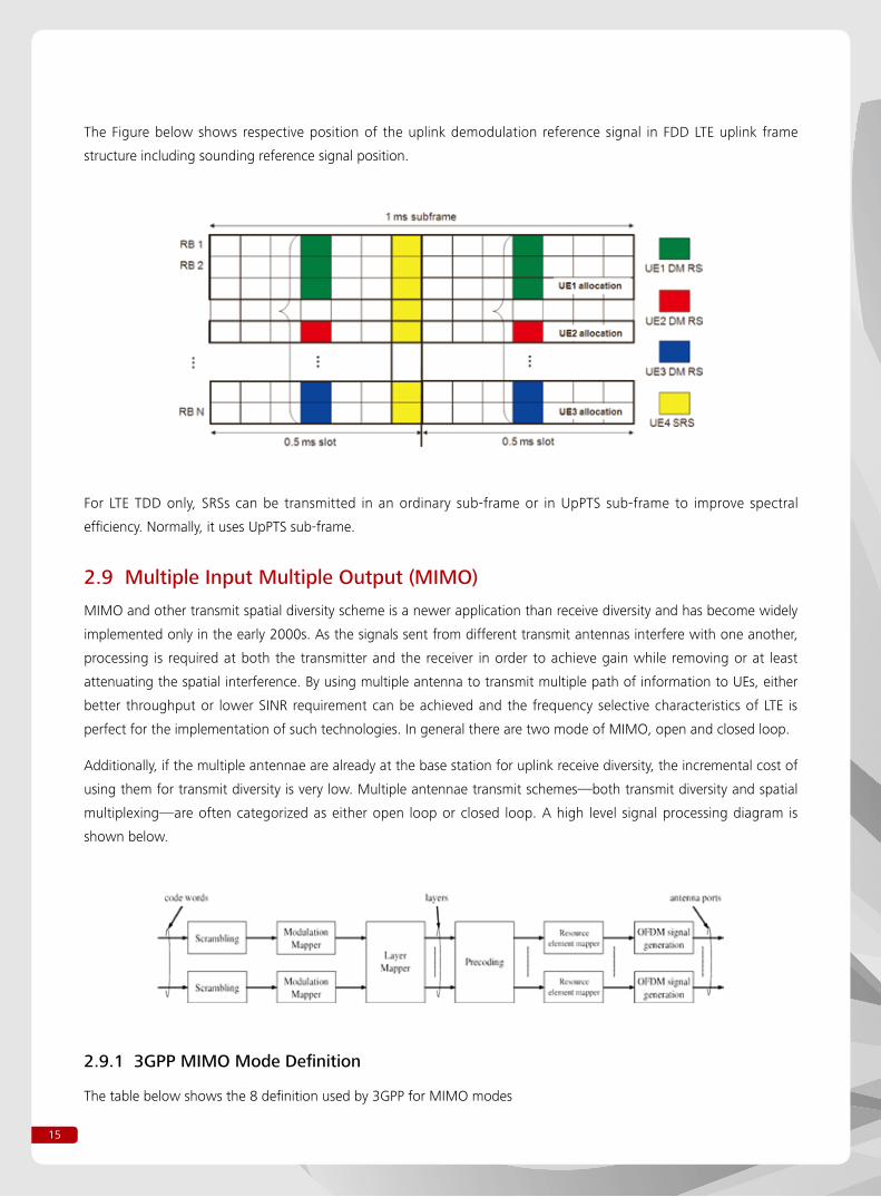
The Figure below shows respective position of the uplink demodulation reference signal in FDD LTE uplink frame
structure including sounding reference signal position.
For LTE TDD only, SRSs can be transmitted in an ordinary sub-frame or in UpPTS sub-frame to improve spectral
efficiency. Normally, it uses UpPTS sub-frame.
2.9 Multiple Input Multiple Output (MIMO)
MIMO and other transmit spatial diversity scheme is a newer application than receive diversity and has become widely
implemented only in the early 2000s. As the signals sent from different transmit antennas interfere with one another,
processing is required at both the transmitter and the receiver in order to achieve gain while removing or at least
attenuating the spatial interference. By using multiple antenna to transmit multiple path of information to UEs, either
better throughput or lower SINR requirement can be achieved and the frequency selective characteristics of LTE is
perfect for the implementation of such technologies. In general there are two mode of MIMO, open and closed loop.
Additionally, if the multiple antennae are already at the base station for uplink receive diversity, the incremental cost of
using them for transmit diversity is very low. Multiple antennae transmit schemes—both transmit diversity and spatial
multiplexing—are often categorized as either open loop or closed loop. A high level signal processing diagram is
shown below.
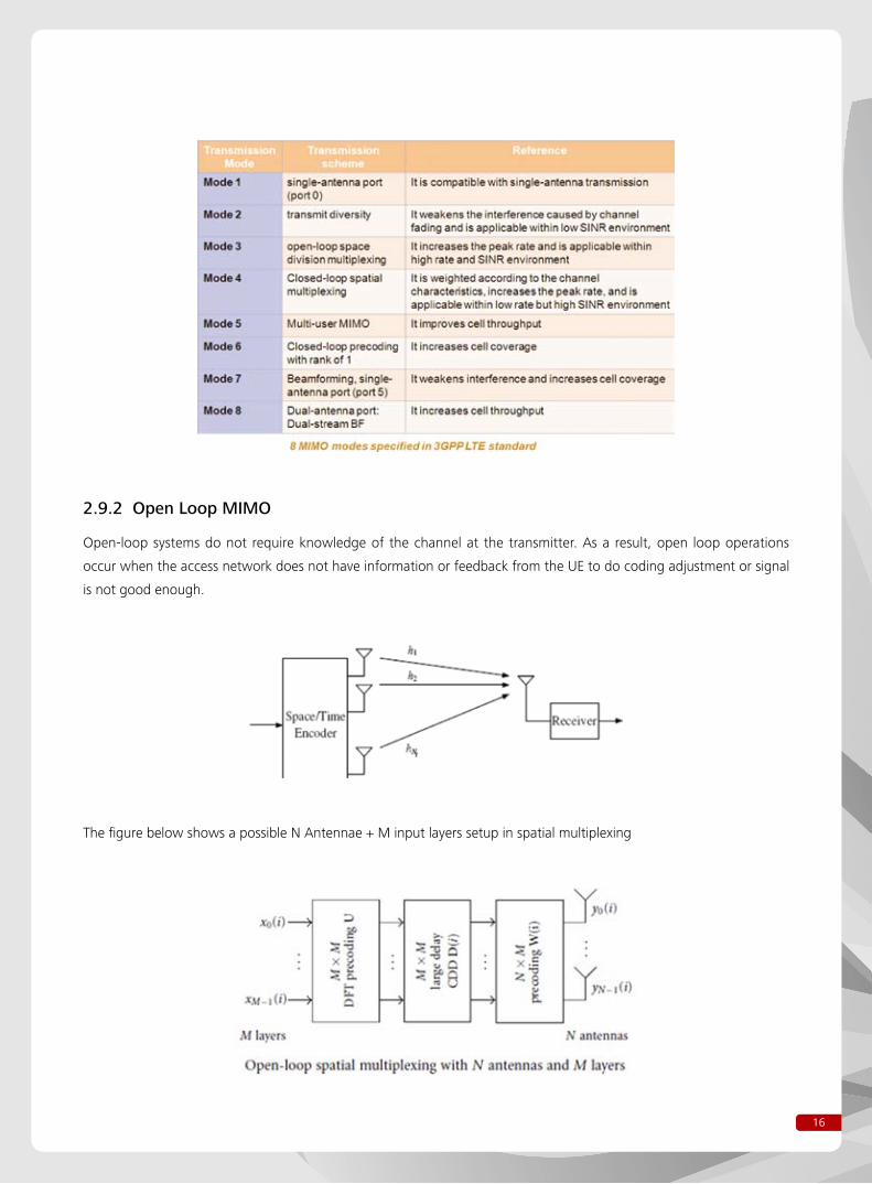
2.9.1 3GPP MIMO Mode Definition
The table below shows the 8 definition used by 3GPP for MIMO modes
16
2.9.2 Open Loop MIMO
Open-loop systems do not require knowledge of the channel at the transmitter. As a result, open loop operations
occur when the access network does not have information or feedback from the UE to do coding adjustment or signal
is not good enough.
The figure below shows a possible N Antennae + M input layers setup in spatial multiplexing
17
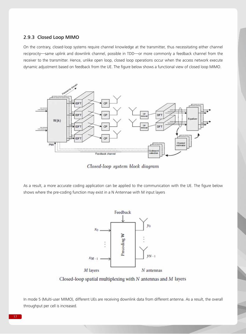
2.9.3 Closed Loop MIMO
On the contrary, closed-loop systems require channel knowledge at the transmitter, thus necessitating either channel
reciprocity—same uplink and downlink channel, possible in TDD—or more commonly a feedback channel from the
receiver to the transmitter. Hence, unlike open loop, closed loop operations occur when the access network execute
dynamic adjustment based on feedback from the UE. The figure below shows a functional view of closed loop MIMO.
As a result, a more accurate coding application can be applied to the communication with the UE. The figure below
shows where the pre-coding function may exist in a N Antennae with M input layers
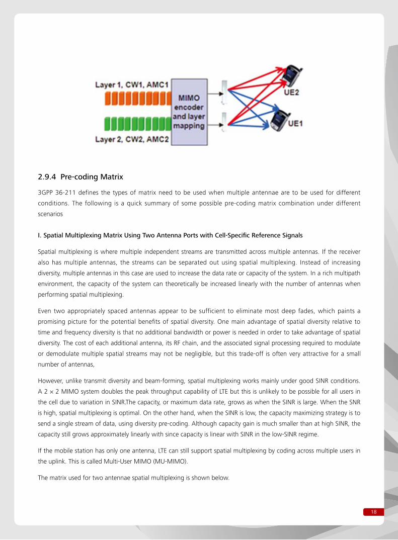
In mode 5 (Multi-user MIMO), different UEs are receiving downlink data from different antenna. As a result, the overall
throughput per cell is increased.
18
2.9.4 Pre-coding Matrix
3GPP 36-211 defines the types of matrix need to be used when multiple antennae are to be used for different
conditions. The following is a quick summary of some possible pre-coding matrix combination under different
scenarios
I. Spatial Multiplexing Matrix Using Two Antenna Ports with Cell-Specific Reference Signals
Spatial multiplexing is where multiple independent streams are transmitted across multiple antennas. If the receiver
also has multiple antennas, the streams can be separated out using spatial multiplexing. Instead of increasing
diversity, multiple antennas in this case are used to increase the data rate or capacity of the system. In a rich multipath
environment, the capacity of the system can theoretically be increased linearly with the number of antennas when
performing spatial multiplexing.
Even two appropriately spaced antennas appear to be sufficient to eliminate most deep fades, which paints a
promising picture for the potential benefits of spatial diversity. One main advantage of spatial diversity relative to
time and frequency diversity is that no additional bandwidth or power is needed in order to take advantage of spatial
diversity. The cost of each additional antenna, its RF chain, and the associated signal processing required to modulate
or demodulate multiple spatial streams may not be negligible, but this trade-off is often very attractive for a small
number of antennas,
However, unlike transmit diversity and beam-forming, spatial multiplexing works mainly under good SINR conditions.
A 2 × 2 MIMO system doubles the peak throughput capability of LTE but this is unlikely to be possible for all users in
the cell due to variation in SINR.The capacity, or maximum data rate, grows as when the SINR is large. When the SNR
is high, spatial multiplexing is optimal. On the other hand, when the SINR is low, the capacity maximizing strategy is to
send a single stream of data, using diversity pre-coding. Although capacity gain is much smaller than at high SINR, the
capacity still grows approximately linearly with since capacity is linear with SINR in the low-SINR regime.
If the mobile station has only one antenna, LTE can still support spatial multiplexing by coding across multiple users in
the uplink. This is called Multi-User MIMO (MU-MIMO).
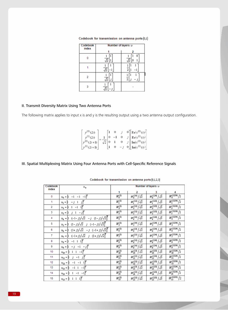
The matrix used for two antennae spatial multiplexing is shown below.
19
II. Transmit Diversity Matrix Using Two Antenna Ports
The following matrix applies to input x is and y is the resulting output using a two antenna output configuration.
III. Spatial Multiplexing Matrix Using Four Antenna Ports with Cell-Specific Reference Signals
20
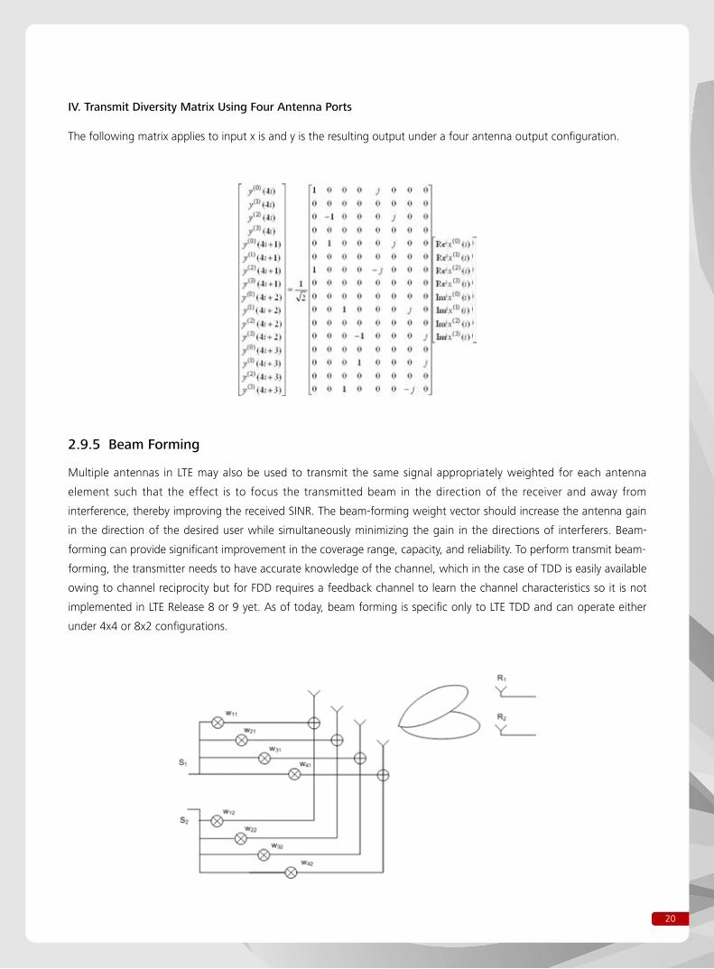
IV. Transmit Diversity Matrix Using Four Antenna Ports
The following matrix applies to input x is and y is the resulting output under a four antenna output configuration.
2.9.5 Beam Forming
Multiple antennas in LTE may also be used to transmit the same signal appropriately weighted for each antenna
element such that the effect is to focus the transmitted beam in the direction of the receiver and away from
interference, thereby improving the received SINR. The beam-forming weight vector should increase the antenna gain
in the direction of the desired user while simultaneously minimizing the gain in the directions of interferers. Beam-
forming can provide significant improvement in the coverage range, capacity, and reliability. To perform transmit beam-
forming, the transmitter needs to have accurate knowledge of the channel, which in the case of TDD is easily available
owing to channel reciprocity but for FDD requires a feedback channel to learn the channel characteristics so it is not
implemented in LTE Release 8 or 9 yet. As of today, beam forming is specific only to LTE TDD and can operate either
under 4x4 or 8x2 configurations.
21
One popular beam-forming algorithm is based on Direction of Arrival where the incoming signals to a receiver may
consist of desired energy and interference energy—for example, from other users or from multipath reflections. The
various signals can be characterized in terms of the DOA or the angle of arrival (AOA) of each received signal. Each
DOA can be estimated by using EUTRAN signal-processing techniques as requested in 3GPP-TS 36-214. From these
acquired DOAs, a beam-former extracts a weighting vector for the antenna elements and uses it to transmit or receive
the desired signal of a specific user while suppressing the undesired interference signals.
Ideally, the beam-former has unity gain for the desired user and two nulls at the directions of two interferers and can
place nulls in the directions of interferers. The DOA-based beam-former in this case is often called the null-steering
beam-former. The null-steering beam-former can be designed to completely cancel out interfering signals only if the
number of such signals is strictly less than the number of antenna elements.
Typically, there exists a trade-off between interference null and desired gain lost. Thus far, we have assumed that the
array response vectors of different users with corresponding AOAs are known. In practice, each resolvable multipath
is likely to comprise several unresolved components coming from significantly different angles. In this case, it is not
possible to associate a discrete AOA with a signal impinging the antenna array. Therefore, the DOA based beam-former
is viable only in LOS environments or in environments with limited local scattering around the transmitter.
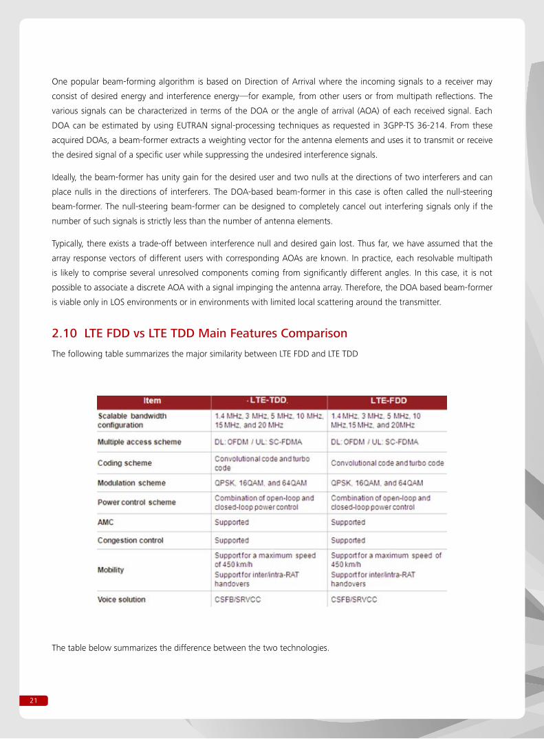
2.10 LTE FDD vs LTE TDD Main Features Comparison
The following table summarizes the major similarity between LTE FDD and LTE TDD
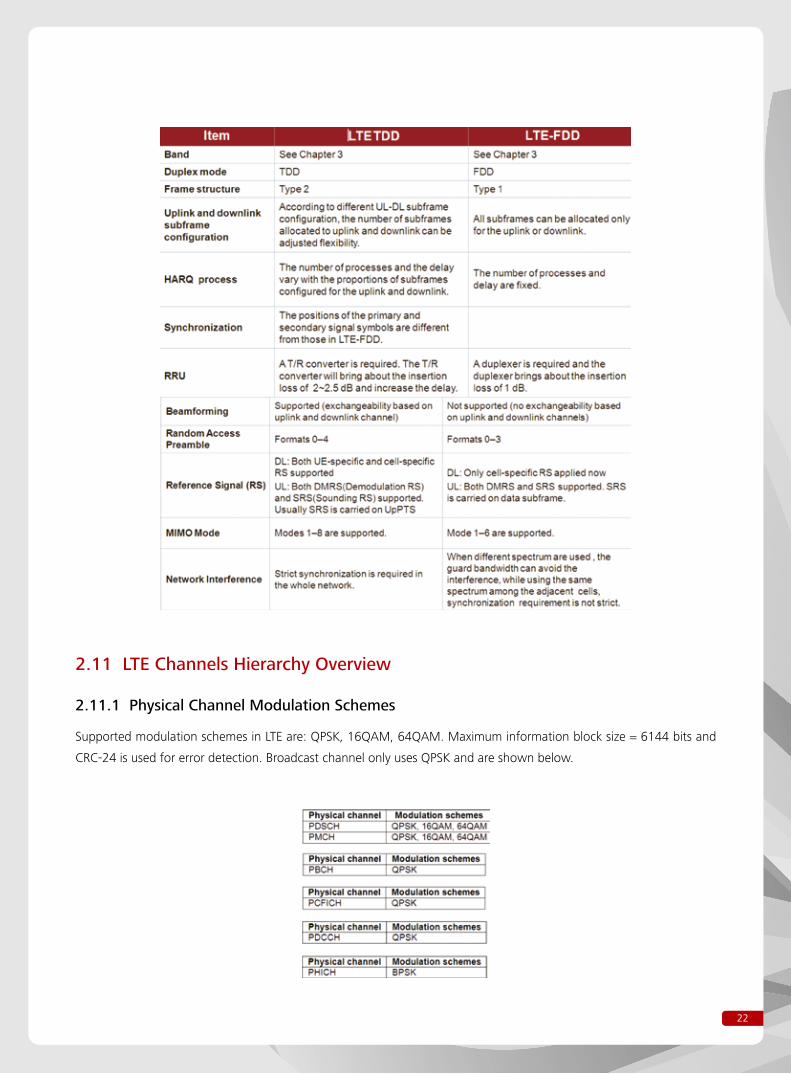
The table below summarizes the difference between the two technologies.
22
2.11 LTE Channels Hierarchy Overview
2.11.1 Physical Channel Modulation Schemes
Supported modulation schemes in LTE are: QPSK, 16QAM, 64QAM. Maximum information block size = 6144 bits and
CRC-24 is used for error detection. Broadcast channel only uses QPSK and are shown below.
23
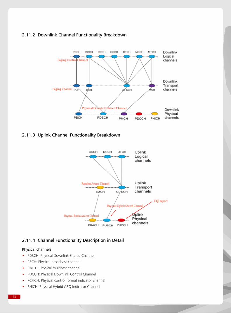
2.11.2 Downlink Channel Functionality Breakdown
2.11.3 Uplink Channel Functionality Breakdown
2.11.4 Channel Functionality Description in Detail
Physical channels
PDSCH: Physical Downlink Shared Channel •
PBCH: Physical broadcast channel •
PMCH: Physical multicast channel •
PDCCH: Physical Downlink Control Channel •
PCFICH: Physical control format indicator channel •
PHICH: Physical Hybrid ARQ Indicator Channel •
24
Reference Signal (RS)
Cell specific RS •
UE-specific RS •
MBSFN RS •
Synchronization Signal (SCH)
Primary Synchronization Signal (P-SCH) •
Secondary Synchronization Signal (S-SCH) •
SCH used for:
Symbol synchronization •
Frame synchronization •
Cell-ID determination •
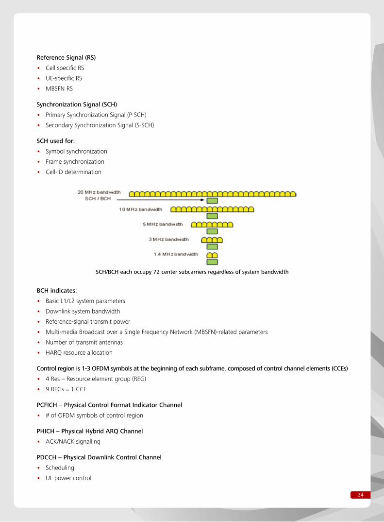
BCH indicates:
Basic L1/L2 system parameters •
Downlink system bandwidth •
Reference-signal transmit power •
Multi-media Broadcast over a Single Frequency Network (MBSFN)-related parameters •
Number of transmit antennas •
HARQ resource allocation •
Control region is 1-3 OFDM symbols at the beginning of each subframe, composed of control channel elements (CCEs)
4 Res = Resource element group (REG) •
9 REGs = 1 CCE •
PCFICH – Physical Control Format Indicator Channel
# of OFDM symbols of control region •
PHICH – Physical Hybrid ARQ Channel
ACK/NACK signalling •
PDCCH – Physical Downlink Control Channel
Scheduling •
UL power control •
SCH/BCH each occupy 72 center subcarriers regardless of system bandwidth
25
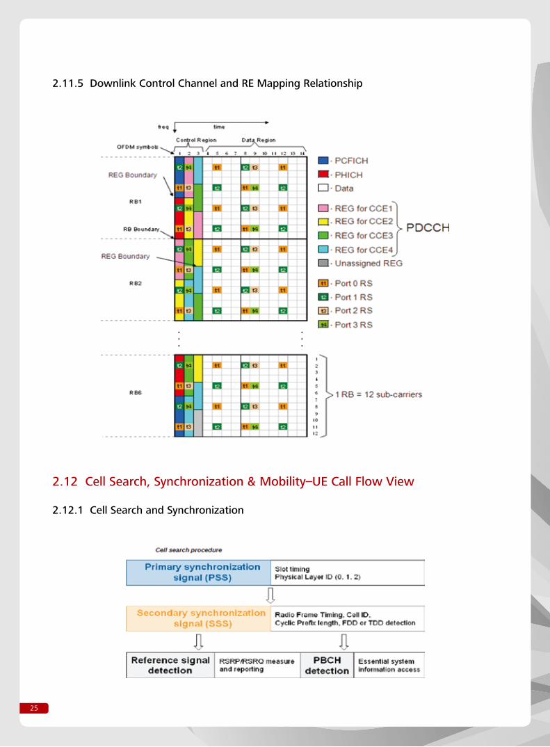
2.11.5 Downlink Control Channel and RE Mapping Relationship
2.12 Cell Search, Synchronization & Mobility–UE Call Flow View
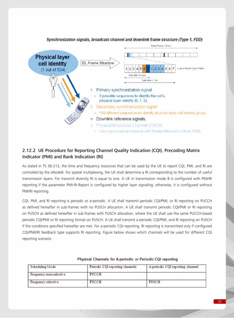
2.12.1 Cell Search and Synchronization
26
2.12.2 UE Procedure for Reporting Channel Quality Indication (CQI), Precoding Matrix Indicator (PMI) and Rank Indication (RI)
As stated in TS 36-213, the time and frequency resources that can be used by the UE to report CQI, PMI, and RI are
controlled by the eNodeB. For spatial multiplexing, the UE shall determine a RI corresponding to the number of useful
transmission layers. For transmit diversity RI is equal to one. A UE in transmission mode 8 is configured with PMI/RI
reporting if the parameter PMI-RI-Report is configured by higher layer signaling; otherwise, it is configured without
PMI/RI reporting.
CQI, PMI, and RI reporting is periodic or a-periodic. A UE shall transmit periodic CQI/PMI, or RI reporting on PUCCH
as defined hereafter in sub-frames with no PUSCH allocation. A UE shall transmit periodic CQI/PMI or RI reporting
on PUSCH as defined hereafter in sub-frames with PUSCH allocation, where the UE shall use the same PUCCH-based
periodic CQI/PMI or RI reporting format on PUSCH. A UE shall transmit a-periodic CQI/PMI, and RI reporting on PUSCH
if the conditions specified hereafter are met. For a-periodic CQI reporting, RI reporting is transmitted only if configured
CQI/PMI/RI feedback type supports RI reporting. Figure below shows which channels will be used for different CQI
reporting scenario
27
2.12.5 EUTRAN Hierarchy and Interface Overview
2.12.4 Mobility Management
2.12.3 System Information Bit Definition
28
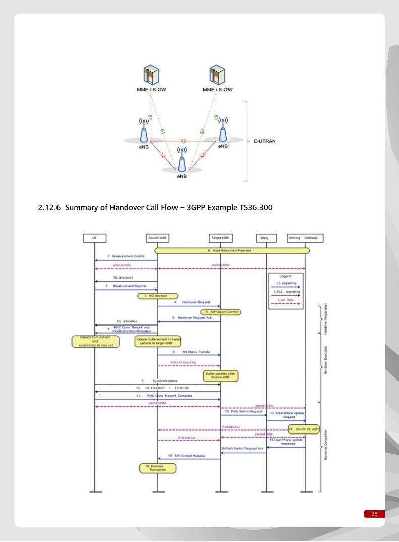
2.12.6 Summary of Handover Call Flow – 3GPP Example TS36.300
29
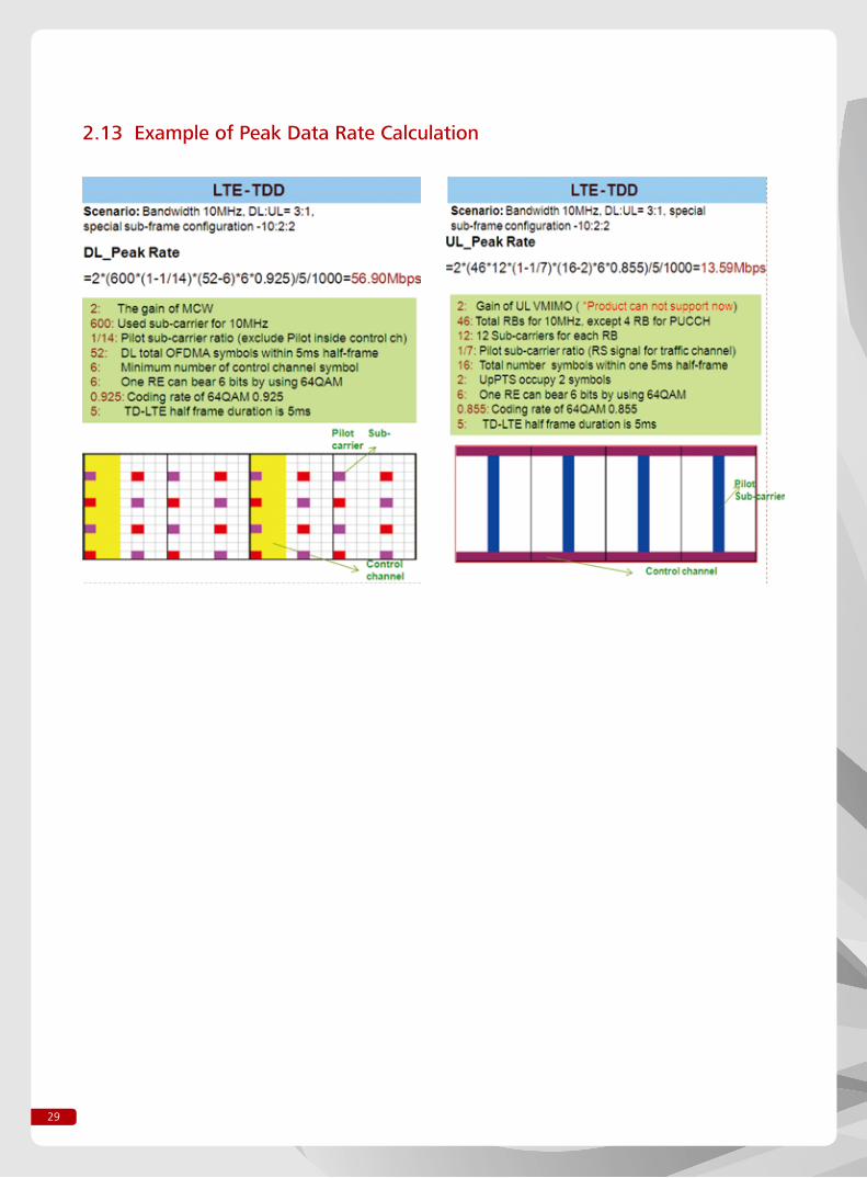
2.13 Example of Peak Data Rate Calculation
30
3 LTE Frequency and Spectrum Planning
3.1 Frequency Spectrum Overview - FDD
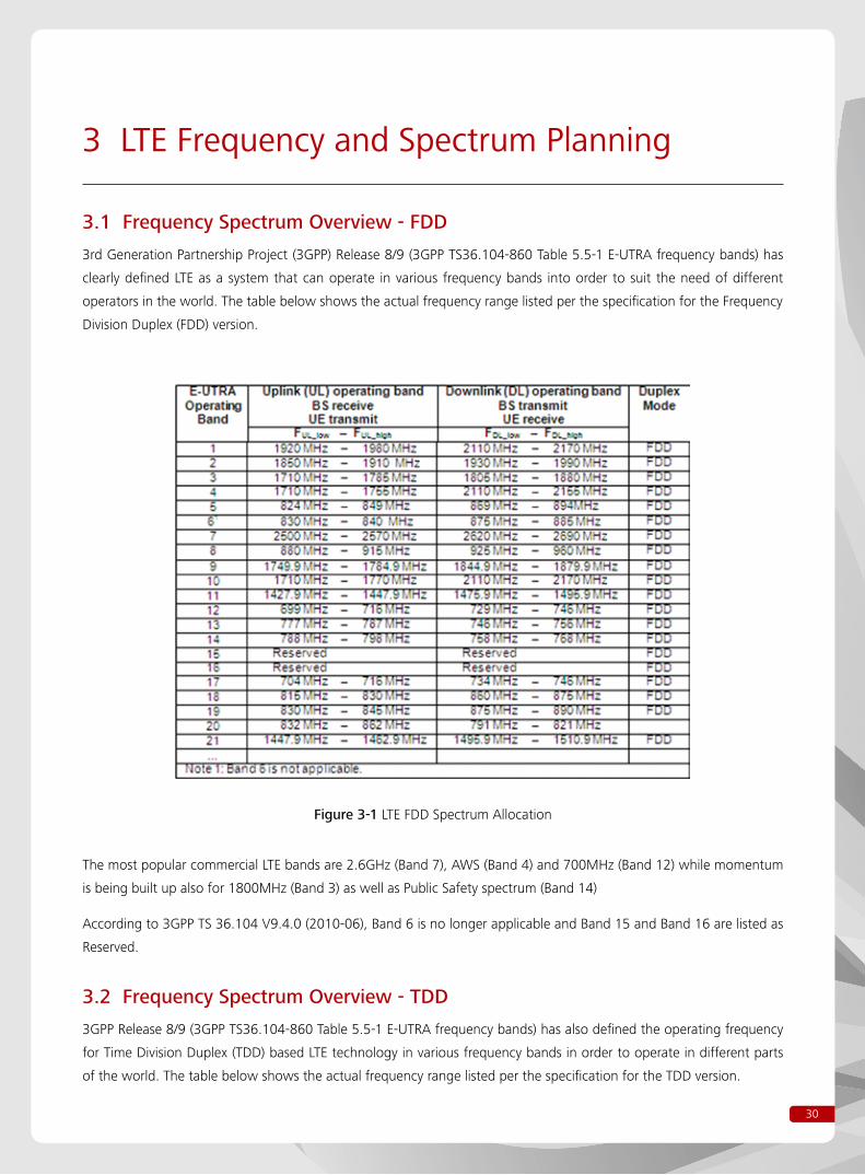
3rd Generation Partnership Project (3GPP) Release 8/9 (3GPP TS36.104-860 Table 5.5-1 E-UTRA frequency bands) has
clearly defined LTE as a system that can operate in various frequency bands into order to suit the need of different
operators in the world. The table below shows the actual frequency range listed per the specification for the Frequency
Division Duplex (FDD) version.
The most popular commercial LTE bands are 2.6GHz (Band 7), AWS (Band 4) and 700MHz (Band 12) while momentum
is being built up also for 1800MHz (Band 3) as well as Public Safety spectrum (Band 14)
According to 3GPP TS 36.104 V9.4.0 (2010-06), Band 6 is no longer applicable and Band 15 and Band 16 are listed as
Reserved.
3.2 Frequency Spectrum Overview - TDD
3GPP Release 8/9 (3GPP TS36.104-860 Table 5.5-1 E-UTRA frequency bands) has also defined the operating frequency
for Time Division Duplex (TDD) based LTE technology in various frequency bands in order to operate in different parts
of the world. The table below shows the actual frequency range listed per the specification for the TDD version.
Figure 3-1 LTE FDD Spectrum Allocation
31
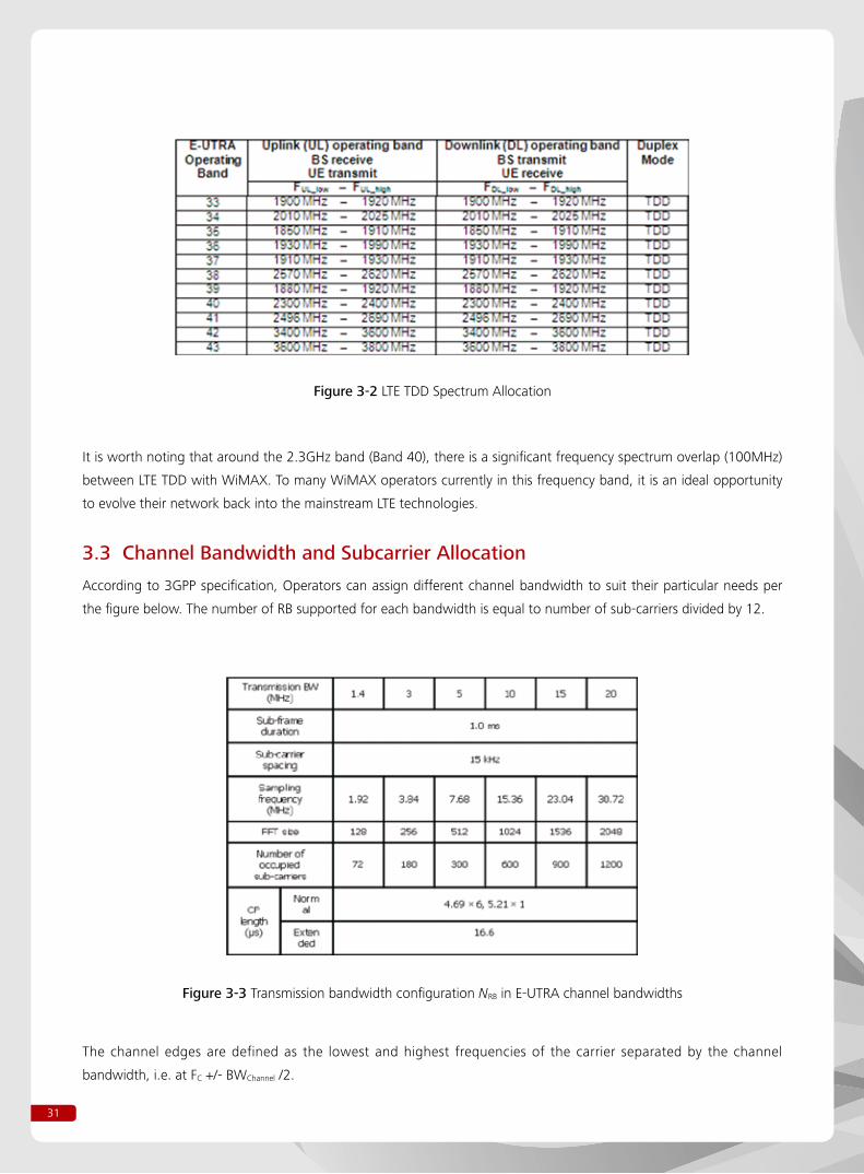
It is worth noting that around the 2.3GHz band (Band 40), there is a significant frequency spectrum overlap (100MHz)
between LTE TDD with WiMAX. To many WiMAX operators currently in this frequency band, it is an ideal opportunity
to evolve their network back into the mainstream LTE technologies.
3.3 Channel Bandwidth and Subcarrier Allocation
According to 3GPP specification, Operators can assign different channel bandwidth to suit their particular needs per
the figure below. The number of RB supported for each bandwidth is equal to number of sub-carriers divided by 12.
Figure 3-2 LTE TDD Spectrum Allocation
Figure 3-3 Transmission bandwidth configuration NRB in E-UTRA channel bandwidths
The channel edges are defined as the lowest and highest frequencies of the carrier separated by the channel
bandwidth, i.e. at FC +/- BWChannel /2.
32
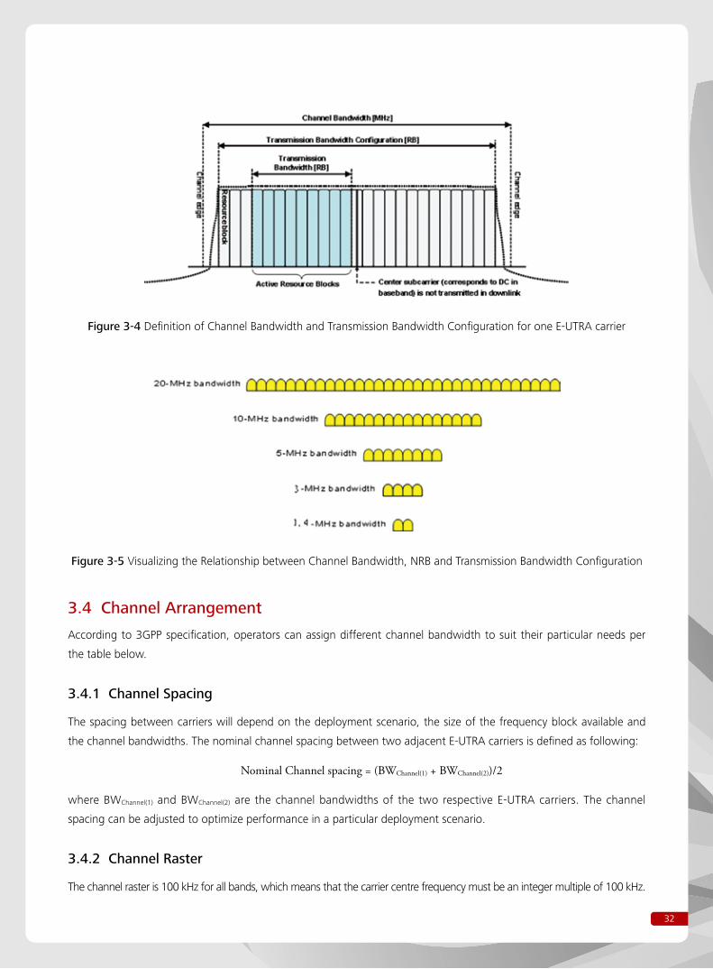
Figure 3-4 Definition of Channel Bandwidth and Transmission Bandwidth Configuration for one E-UTRA carrier
Figure 3-5 Visualizing the Relationship between Channel Bandwidth, NRB and Transmission Bandwidth Configuration
3.4 Channel Arrangement
According to 3GPP specification, operators can assign different channel bandwidth to suit their particular needs per
the table below.
3.4.1 Channel Spacing
The spacing between carriers will depend on the deployment scenario, the size of the frequency block available and
the channel bandwidths. The nominal channel spacing between two adjacent E-UTRA carriers is defined as following:
Nominal Channel spacing = (BWChannel(1) + BWChannel(2))/2
where BWChannel(1) and BWChannel(2) are the channel bandwidths of the two respective E-UTRA carriers. The channel
spacing can be adjusted to optimize performance in a particular deployment scenario.
3.4.2 Channel Raster
The channel raster is 100 kHz for all bands, which means that the carrier centre frequency must be an integer multiple of 100 kHz.
33
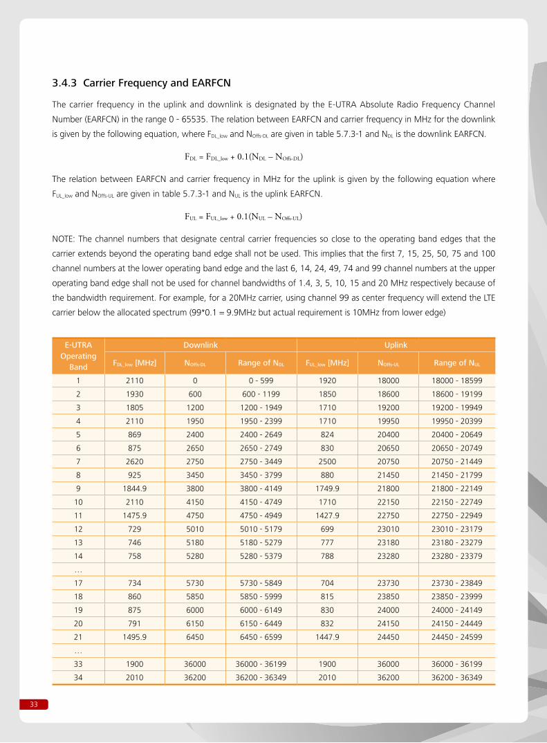
3.4.3 Carrier Frequency and EARFCN
The carrier frequency in the uplink and downlink is designated by the E-UTRA Absolute Radio Frequency Channel
Number (EARFCN) in the range 0 - 65535. The relation between EARFCN and carrier frequency in MHz for the downlink
is given by the following equation, where FDL_low and NOffs-DL are given in table 5.7.3-1 and NDL is the downlink EARFCN.
FDL = FDL_low + 0.1(NDL – NOffs-DL)
The relation between EARFCN and carrier frequency in MHz for the uplink is given by the following equation where
FUL_low and NOffs-UL are given in table 5.7.3-1 and NUL is the uplink EARFCN.
FUL = FUL_low + 0.1(NUL – NOffs-UL)
NOTE: The channel numbers that designate central carrier frequencies so close to the operating band edges that the
carrier extends beyond the operating band edge shall not be used. This implies that the first 7, 15, 25, 50, 75 and 100
channel numbers at the lower operating band edge and the last 6, 14, 24, 49, 74 and 99 channel numbers at the upper
operating band edge shall not be used for channel bandwidths of 1.4, 3, 5, 10, 15 and 20 MHz respectively because of
the bandwidth requirement. For example, for a 20MHz carrier, using channel 99 as center frequency will extend the LTE
carrier below the allocated spectrum (99*0.1 = 9.9MHz but actual requirement is 10MHz from lower edge)
E-UTRA Operating
Band
Downlink Uplink
FDL_low [MHz] NOffs-DL Range of NDL FUL_low [MHz] NOffs-UL Range of NUL
1 2110 0 0 - 599 1920 18000 18000 - 18599
2 1930 600 600 - 1199 1850 18600 18600 - 19199
3 1805 1200 1200 - 1949 1710 19200 19200 - 19949
4 2110 1950 1950 - 2399 1710 19950 19950 - 20399
5 869 2400 2400 - 2649 824 20400 20400 - 20649
6 875 2650 2650 - 2749 830 20650 20650 - 20749
7 2620 2750 2750 - 3449 2500 20750 20750 - 21449
8 925 3450 3450 - 3799 880 21450 21450 - 21799
9 1844.9 3800 3800 - 4149 1749.9 21800 21800 - 22149
10 2110 4150 4150 - 4749 1710 22150 22150 - 22749
11 1475.9 4750 4750 - 4949 1427.9 22750 22750 - 22949
12 729 5010 5010 - 5179 699 23010 23010 - 23179
13 746 5180 5180 - 5279 777 23180 23180 - 23279
14 758 5280 5280 - 5379 788 23280 23280 - 23379
…
17 734 5730 5730 - 5849 704 23730 23730 - 23849
18 860 5850 5850 - 5999 815 23850 23850 - 23999
19 875 6000 6000 - 6149 830 24000 24000 - 24149
20 791 6150 6150 - 6449 832 24150 24150 - 24449
21 1495.9 6450 6450 - 6599 1447.9 24450 24450 - 24599
…
33 1900 36000 36000 - 36199 1900 36000 36000 - 36199
34 2010 36200 36200 - 36349 2010 36200 36200 - 36349
34
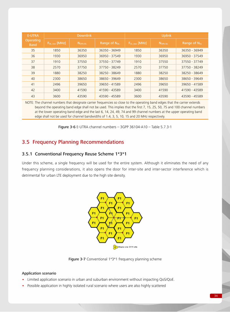
Figure 3-6 E-UTRA channel numbers – 3GPP 36104-A10 – Table 5.7.3-1
E-UTRA Operating
Band
Downlink Uplink
FDL_low [MHz] NOffs-DL Range of NDL FUL_low [MHz] NOffs-UL Range of NUL
35 1850 36350 36350 - 36949 1850 36350 36350 - 36949
36 1930 36950 36950 - 37549 1930 36950 36950 - 37549
37 1910 37550 37550 - 37749 1910 37550 37550 - 37749
38 2570 37750 37750 - 38249 2570 37750 37750 - 38249
39 1880 38250 38250 - 38649 1880 38250 38250 - 38649
40 2300 38650 38650 - 39649 2300 38650 38650 - 39649
41 2496 39650 39650 - 41589 2496 39650 39650 - 41589
42 3400 41590 41590 - 43589 3400 41590 41590 - 43589
43 3600 43590 43590 - 45589 3600 43590 43590 - 45589
NOTE: The channel numbers that designate carrier frequencies so close to the operating band edges that the carrier extends beyond the operating band edge shall not be used. This implies that the first 7, 15, 25, 50, 75 and 100 channel numbers at the lower operating band edge and the last 6, 14, 24, 49, 74 and 99 channel numbers at the upper operating band edge shall not be used for channel bandwidths of 1.4, 3, 5, 10, 15 and 20 MHz respectively.
3.5 Frequency Planning Recommendations
3.5.1 Conventional Frequency Reuse Scheme 1*3*1
Under this scheme, a single frequency will be used for the entire system. Although it eliminates the need of any
frequency planning considerations, it also opens the door for inter-site and inter-sector interference which is
detrimental for urban LTE deployment due to the high site density.
Figure 3-7 Conventional 1*3*1 frequency planning scheme
Application scenario
Limited application scenario in urban and suburban environment without impacting QoS/QoE. •
Possible application in highly isolated rural scenario where users are also highly scattered •
35
Advantage
High spectral efficiency and high throughput per site. •
Easy to deploy. •
No special scheduling algorithm required •
Disadvantage
High level of interference especially on cell edge area •
Low throughput on cell boundary and lower QoS/QoE for users on boundary area. •
Coverage control of cells becomes an important factor in achieving a high throughput level •
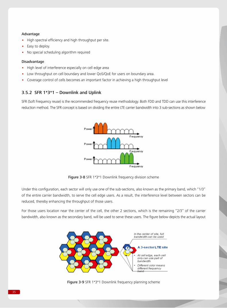
3.5.2 SFR 1*3*1 – Downlink and Uplink
SFR (Soft Frequency reuse) is the recommended frequency reuse methodology. Both FDD and TDD can use this interference
reduction method. The SFR concept is based on dividing the entire LTE carrier bandwidth into 3 sub-sections as shown below
Under this configuration, each sector will only use one of the sub-sections, also known as the primary band, which “1/3”
of the entire carrier bandwidth, to serve the cell edge users. As a result, the interference level between sectors can be
reduced, thereby enhancing the throughput of those users.
For those users location near the center of the cell, the other 2 sections, which is the remaining “2/3” of the carrier
bandwidth, also known as the secondary band, will be used to serve these users. The figure below depicts the actual layout
Figure 3-8 SFR 1*3*1 Downlink frequency division scheme
Figure 3-9 SFR 1*3*1 Downlink frequency planning scheme
36
Application scenario
Recommended configuration to satisfy high traffic and high site density requirement. •
Best results will require the introduction of Inter Cell Interference Coordination (ICIC) •
Advantage
Reduce inter-cell interference under a high site density deployment. •
Improve cell edge user throughput and quality of experience. •
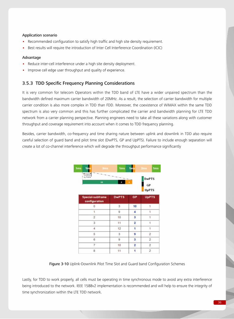
3.5.3 TDD Specific Frequency Planning Considerations
It is very common for telecom Operators within the TDD band of LTE have a wider unpaired spectrum than the
bandwidth defined maximum carrier bandwidth of 20MHz. As a result, the selection of carrier bandwidth for multiple
carrier condition is also more complex in TDD than FDD. Moreover, the coexistence of WiMAX within the same TDD
spectrum is also very common and this has further complicated the carrier and bandwidth planning for LTE TDD
network from a carrier planning perspective. Planning engineers need to take all these variations along with customer
throughput and coverage requirement into account when it comes to TDD frequency planning.
Besides, carrier bandwidth, co-frequency and time sharing nature between uplink and downlink in TDD also require
careful selection of guard band and pilot time slot (DwPTS, GP and UpPTS). Failure to include enough separation will
create a lot of co-channel interference which will degrade the throughput performance significantly
Figure 3-10 Uplink-Downlink Pilot Time Slot and Guard band Configuration Schemes
Lastly, for TDD to work properly, all cells must be operating in time synchronous mode to avoid any extra interference
being introduced to the network. IEEE 1588v2 implementation is recommended and will help to ensure the integrity of
time synchronization within the LTE TDD network.
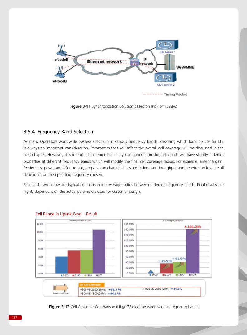
37
3.5.4 Frequency Band Selection
As many Operators worldwide possess spectrum in various frequency bands, choosing which band to use for LTE
is always an important consideration. Parameters that will affect the overall cell coverage will be discussed in the
next chapter. However, it is important to remember many components on the radio path will have slightly different
properties at different frequency bands which will modify the final cell coverage radius. For example, antenna gain,
feeder loss, power amplifier output, propagation characteristics, cell edge user throughput and penetration loss are all
dependent on the operating frequency chosen.
Results shown below are typical comparison in coverage radius between different frequency bands. Final results are
highly dependent on the actual parameters used for customer design.
Figure 3-11 Synchronization Solution based on IPclk or 1588v2
Figure 3-12 Cell Coverage Comparison (UL@128kbps) between various frequency bands
Cell Range in Uplink Case -- Result
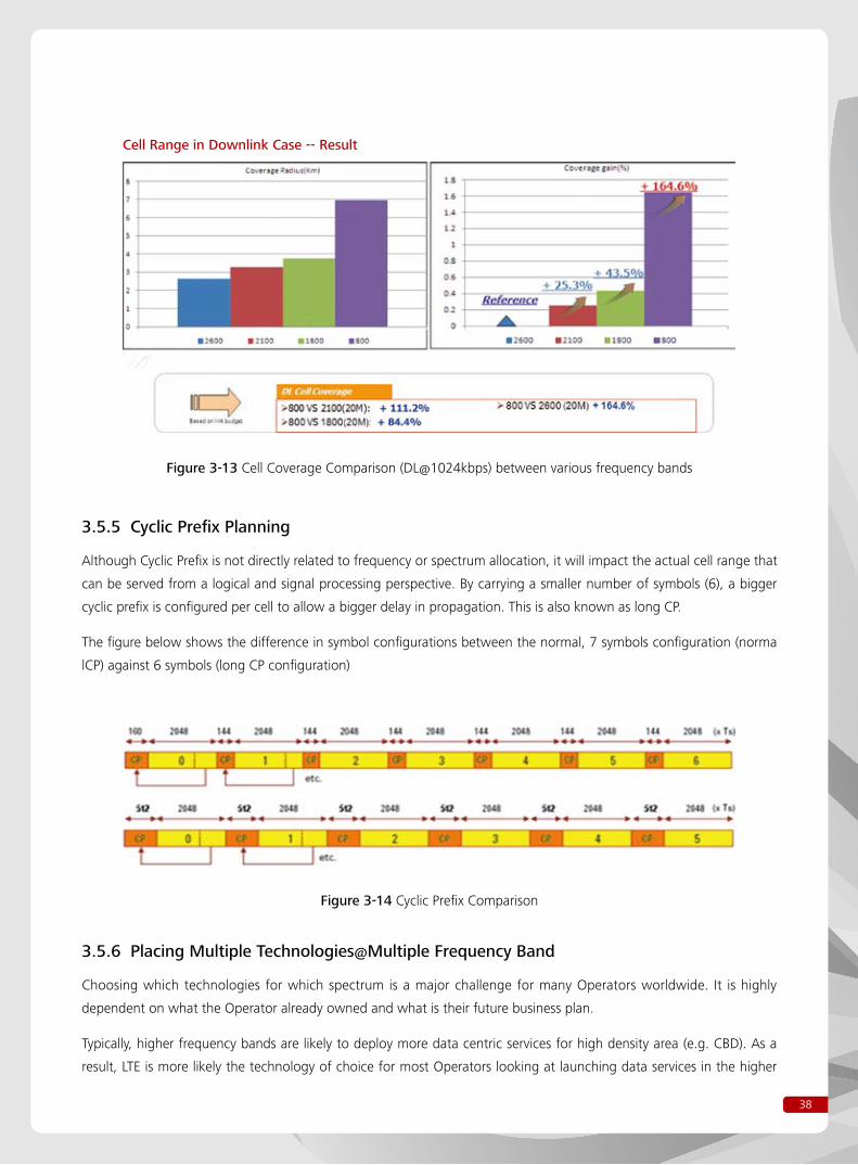
38
Cell Range in Downlink Case -- Result
Figure 3-13 Cell Coverage Comparison (DL@1024kbps) between various frequency bands
3.5.5 Cyclic Prefix Planning
Although Cyclic Prefix is not directly related to frequency or spectrum allocation, it will impact the actual cell range that
can be served from a logical and signal processing perspective. By carrying a smaller number of symbols (6), a bigger
cyclic prefix is configured per cell to allow a bigger delay in propagation. This is also known as long CP.
The figure below shows the difference in symbol configurations between the normal, 7 symbols configuration (norma
lCP) against 6 symbols (long CP configuration)
Figure 3-14 Cyclic Prefix Comparison
3.5.6 Placing Multiple Technologies@Multiple Frequency Band
Choosing which technologies for which spectrum is a major challenge for many Operators worldwide. It is highly
dependent on what the Operator already owned and what is their future business plan.
Typically, higher frequency bands are likely to deploy more data centric services for high density area (e.g. CBD). As a
result, LTE is more likely the technology of choice for most Operators looking at launching data services in the higher
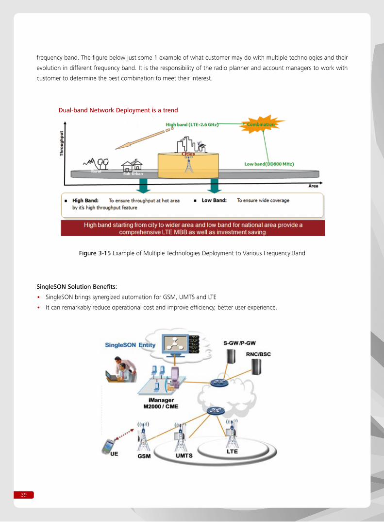
39
frequency band. The figure below just some 1 example of what customer may do with multiple technologies and their
evolution in different frequency band. It is the responsibility of the radio planner and account managers to work with
customer to determine the best combination to meet their interest.
SingleSON Solution Benefits:
SingleSON brings synergized automation for GSM, UMTS and LTE •
It can remarkably reduce operational cost and improve efficiency, better user experience. •
Dual-band Network Deployment is a trend
Figure 3-15 Example of Multiple Technologies Deployment to Various Frequency Band
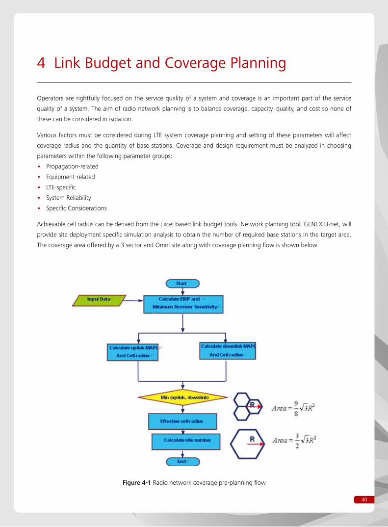
40
Figure 4-1 Radio network coverage pre-planning flow
4 Link Budget and Coverage Planning
Operators are rightfully focused on the service quality of a system and coverage is an important part of the service
quality of a system. The aim of radio network planning is to balance coverage, capacity, quality, and cost so none of
these can be considered in isolation.
Various factors must be considered during LTE system coverage planning and setting of these parameters will affect
coverage radius and the quantity of base stations. Coverage and design requirement must be analyzed in choosing
parameters within the following parameter groups:
Propagation-related •
Equipment-related •
LTE-specific •
System Reliability •
Specific Considerations •
Achievable cell radius can be derived from the Excel based link budget tools. Network planning tool, GENEX U-net, will
provide site deployment specific simulation analysis to obtain the number of required base stations in the target area.
The coverage area offered by a 3 sector and Omni site along with coverage planning flow is shown below
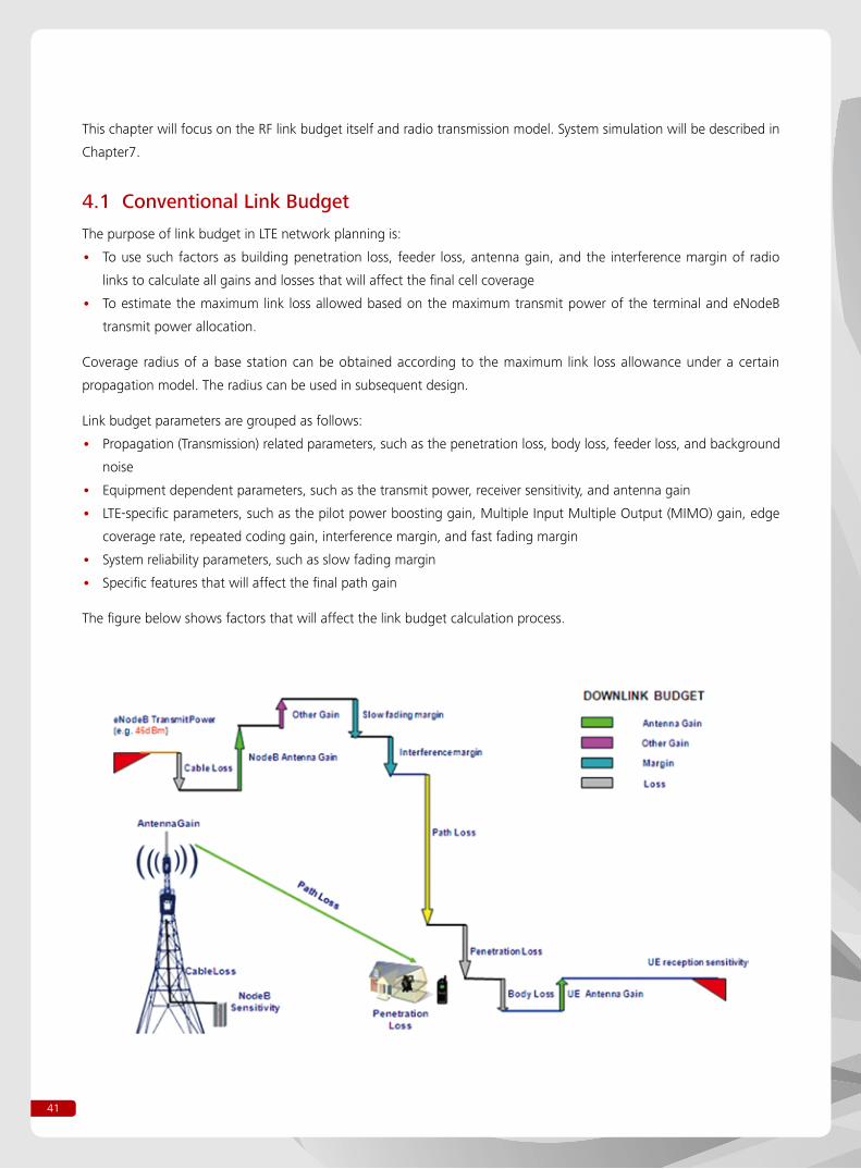
41
This chapter will focus on the RF link budget itself and radio transmission model. System simulation will be described in
Chapter7.
4.1 Conventional Link Budget
The purpose of link budget in LTE network planning is:
To use such factors as building penetration loss, feeder loss, antenna gain, and the interference margin of radio •
links to calculate all gains and losses that will affect the final cell coverage
To estimate the maximum link loss allowed based on the maximum transmit power of the terminal and eNodeB •
transmit power allocation.
Coverage radius of a base station can be obtained according to the maximum link loss allowance under a certain
propagation model. The radius can be used in subsequent design.
Link budget parameters are grouped as follows:
Propagation (Transmission) related parameters, such as the penetration loss, body loss, feeder loss, and background •
noise
Equipment dependent parameters, such as the transmit power, receiver sensitivity, and antenna gain •
LTE-specific parameters, such as the pilot power boosting gain, Multiple Input Multiple Output (MIMO) gain, edge •
coverage rate, repeated coding gain, interference margin, and fast fading margin
System reliability parameters, such as slow fading margin •
Specific features that will affect the final path gain •
The figure below shows factors that will affect the link budget calculation process.
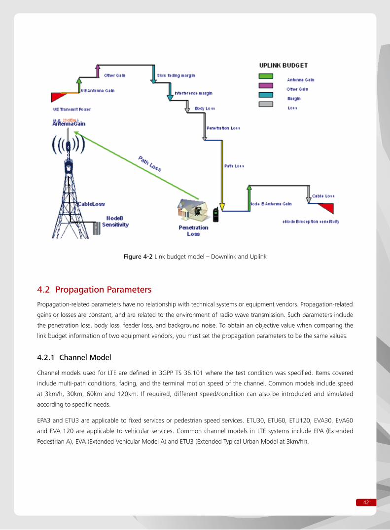
42
Figure 4-2 Link budget model – Downlink and Uplink
4.2 Propagation Parameters
Propagation-related parameters have no relationship with technical systems or equipment vendors. Propagation-related
gains or losses are constant, and are related to the environment of radio wave transmission. Such parameters include
the penetration loss, body loss, feeder loss, and background noise. To obtain an objective value when comparing the
link budget information of two equipment vendors, you must set the propagation parameters to be the same values.
4.2.1 Channel Model
Channel models used for LTE are defined in 3GPP TS 36.101 where the test condition was specified. Items covered
include multi-path conditions, fading, and the terminal motion speed of the channel. Common models include speed
at 3km/h, 30km, 60km and 120km. If required, different speed/condition can also be introduced and simulated
according to specific needs.
EPA3 and ETU3 are applicable to fixed services or pedestrian speed services. ETU30, ETU60, ETU120, EVA30, EVA60
and EVA 120 are applicable to vehicular services. Common channel models in LTE systems include EPA (Extended
Pedestrian A), EVA (Extended Vehicular Model A) and ETU3 (Extended Typical Urban Model at 3km/hr).
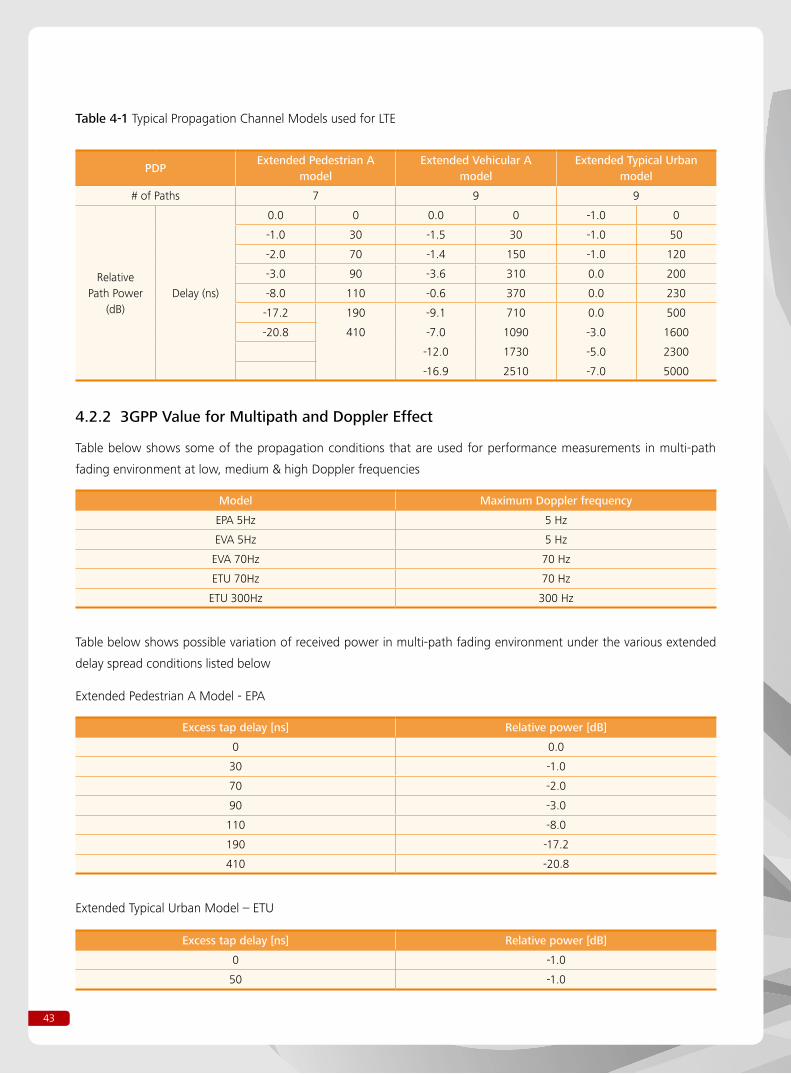
43
PDPExtended Pedestrian A
model Extended Vehicular A
modelExtended Typical Urban
model
# of Paths 7 9 9
Relative Path Power
(dB) Delay (ns)
0.0 0 0.0 0 -1.0 0
-1.0 30 -1.5 30 -1.0 50
-2.0 70 -1.4 150 -1.0 120
-3.0 90 -3.6 310 0.0 200
-8.0 110 -0.6 370 0.0 230
-17.2 190 -9.1 710 0.0 500
-20.8 410 -7.0 1090 -3.0 1600
-12.0 1730 -5.0 2300
-16.9 2510 -7.0 5000
Table 4-1 Typical Propagation Channel Models used for LTE
4.2.2 3GPP Value for Multipath and Doppler Effect
Table below shows some of the propagation conditions that are used for performance measurements in multi-path
fading environment at low, medium & high Doppler frequencies
Model Maximum Doppler frequency
EPA 5Hz 5 Hz
EVA 5Hz 5 Hz
EVA 70Hz 70 Hz
ETU 70Hz 70 Hz
ETU 300Hz 300 Hz
Excess tap delay [ns] Relative power [dB]
0 0.0
30 -1.0
70 -2.0
90 -3.0
110 -8.0
190 -17.2
410 -20.8
Table below shows possible variation of received power in multi-path fading environment under the various extended
delay spread conditions listed below
Extended Pedestrian A Model - EPA
Excess tap delay [ns] Relative power [dB]
0 -1.0
50 -1.0
Extended Typical Urban Model – ETU
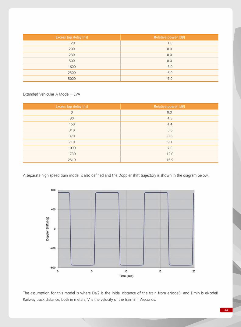
44
Excess tap delay [ns] Relative power [dB]
0 0.0
30 -1.5
150 -1.4
310 -3.6
370 -0.6
710 -9.1
1090 -7.0
1730 -12.0
2510 -16.9
Extended Vehicular A Model – EVA
A separate high speed train model is also defined and the Doppler shift trajectory is shown in the diagram below.
Excess tap delay [ns] Relative power [dB]
120 -1.0
200 0.0
230 0.0
500 0.0
1600 -3.0
2300 -5.0
5000 -7.0
The assumption for this model is where Ds/2 is the initial distance of the train from eNodeB, and Dmin is eNodeB
Railway track distance, both in meters; V is the velocity of the train in m/seconds.
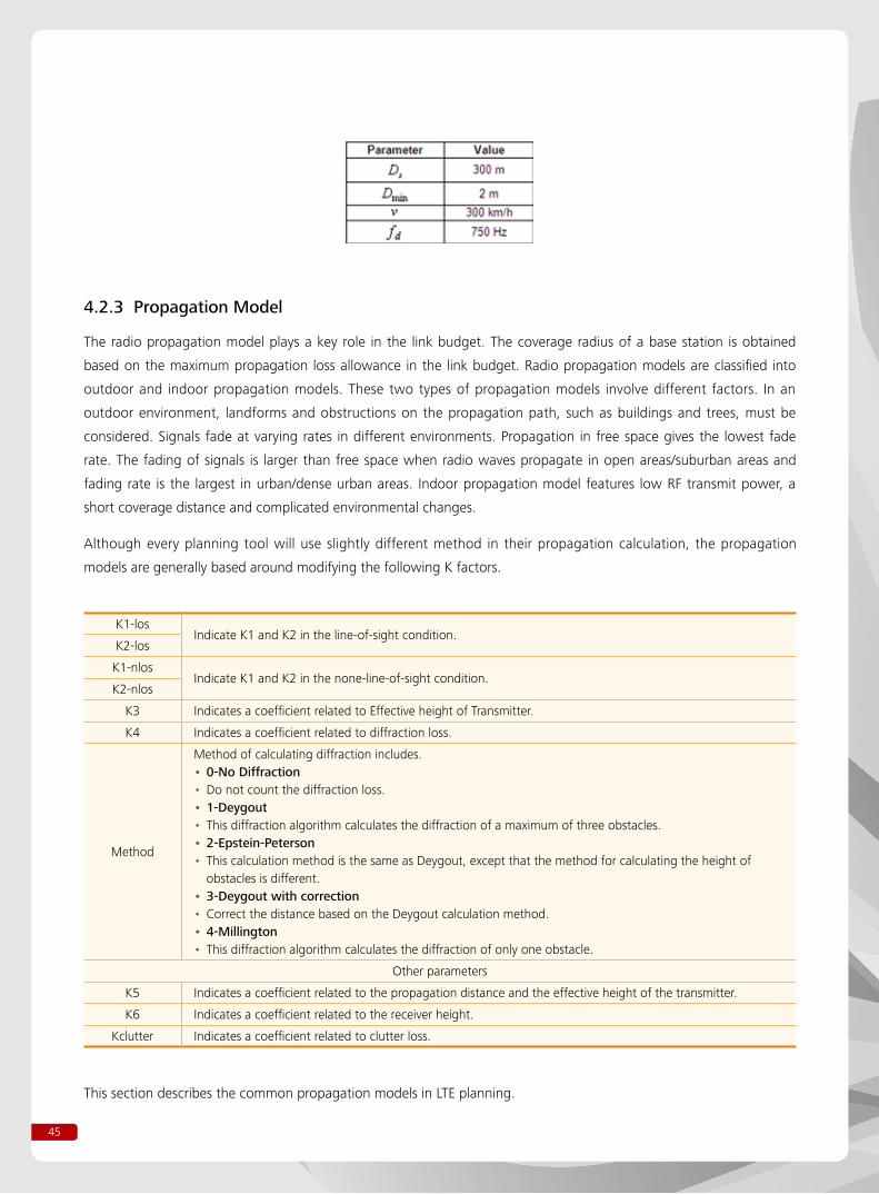
45
4.2.3 Propagation Model
The radio propagation model plays a key role in the link budget. The coverage radius of a base station is obtained
based on the maximum propagation loss allowance in the link budget. Radio propagation models are classified into
outdoor and indoor propagation models. These two types of propagation models involve different factors. In an
outdoor environment, landforms and obstructions on the propagation path, such as buildings and trees, must be
considered. Signals fade at varying rates in different environments. Propagation in free space gives the lowest fade
rate. The fading of signals is larger than free space when radio waves propagate in open areas/suburban areas and
fading rate is the largest in urban/dense urban areas. Indoor propagation model features low RF transmit power, a
short coverage distance and complicated environmental changes.
Although every planning tool will use slightly different method in their propagation calculation, the propagation
models are generally based around modifying the following K factors.
K1-losIndicate K1 and K2 in the line-of-sight condition.
K2-los
K1-nlosIndicate K1 and K2 in the none-line-of-sight condition.
K2-nlos
K3 Indicates a coefficient related to Effective height of Transmitter.
K4 Indicates a coefficient related to diffraction loss.
Method
Method of calculating diffraction includes.0-No Diffraction• Do not count the diffraction loss.• 1-Deygout• This diffraction algorithm calculates the diffraction of a maximum of three obstacles.• 2-Epstein-Peterson• This calculation method is the same as Deygout, except that the method for calculating the height of • obstacles is different.3-Deygout with correction• Correct the distance based on the Deygout calculation method.• 4-Millington• This diffraction algorithm calculates the diffraction of only one obstacle.•
Other parameters
K5 Indicates a coefficient related to the propagation distance and the effective height of the transmitter.
K6 Indicates a coefficient related to the receiver height.
Kclutter Indicates a coefficient related to clutter loss.
This section describes the common propagation models in LTE planning.
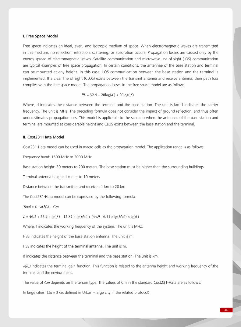
46
I. Free Space Model
Free space indicates an ideal, even, and isotropic medium of space. When electromagnetic waves are transmitted
in this medium, no reflection, refraction, scattering, or absorption occurs. Propagation losses are caused only by the
energy spread of electromagnetic waves. Satellite communication and microwave line-of-sight (LOS) communication
are typical examples of free space propagation. In certain conditions, the antennae of the base station and terminal
can be mounted at any height. In this case, LOS communication between the base station and the terminal is
implemented. If a clear line of sight (CLOS) exists between the transmit antenna and receive antenna, then path loss
complies with the free space model. The propagation losses in the free space model are as follows:
PL = 32.4 + 20log(d ) + 20log( f )
Where, d indicates the distance between the terminal and the base station. The unit is km. f indicates the carrier
frequency. The unit is MHz. The preceding formula does not consider the impact of ground reflection, and thus often
underestimates propagation loss. This model is applicable to the scenario when the antennas of the base station and
terminal are mounted at considerable height and CLOS exists between the base station and the terminal.
II. Cost231-Hata Model
Cost231-Hata model can be used in macro cells as the propagation model. The application range is as follows:
Frequency band: 1500 MHz to 2000 MHz
Base station height: 30 meters to 200 meters. The base station must be higher than the surrounding buildings.
Terminal antenna height: 1 meter to 10 meters
Distance between the transmitter and receiver: 1 km to 20 km
The Cost231-Hata model can be expressed by the following formula:
Total = L - a(Hss) + Cm
L = 46.3 + 33.9 × lg( f ) - 13.82 × lg(HBS) + (44.9 - 6.55 × lg(HBS)) × lg(d )
Where, f indicates the working frequency of the system. The unit is MHz.
HBS indicates the height of the base station antenna. The unit is m.
HSS indicates the height of the terminal antenna. The unit is m.
d indicates the distance between the terminal and the base station. The unit is km.
a(hss) indicates the terminal gain function. This function is related to the antenna height and working frequency of the
terminal and the environment.
The value of Cm depends on the terrain type. The values of Cm in the standard Cost231-Hata are as follows:
In large cities: Cm = 3 (as defined in Urban - large city in the related protocol)
47
In medium-sized cities: Cm = 0 (as defined in Urban – small city in the related protocol)
In suburban areas: Cm = -2(log( f /28))2 - 5.4dB (as defined in Urban – Suburban in the related protocol)
In rural open areas: Cm = -4.78 × (lg( f ))2 + 18.33 × lg( f ) -40.94
(As defined in Rural (open) – desert in the related protocol)
In highways: Cm = -4.78 × (lg( f ))2 + 18.33 × lg( f ) -35.94
(As defined in Rural (quasi-open) – countryside where the terminal is unobstructed for 100 meters in the front in the
related protocol)
Since some of the working frequencies of the LTE networks are 2.3 GHz and 2.6 GHz have exceeded the band range
of the standard Cost 231-Hata model, that is, 150 MHz to 2000 MHz. Therefore, in the actual LTE system design, the
standard Cost231-Hata model must be corrected based on the CW test result. According to the planning experience
and actual CW test results in multiple scenarios, a set of Cm has been created in the experienced model.
III. Standard Propagation Model (SPM)
The standard propagation model is a model (deduced from the Hata formula) particularly suitable for predication
in the 150MHz~3500MHz band over long distance (1Km<d<20Km) and is very adapted to GSM900/1800, UMTS,
CDMA2000, WiMAX and LTE technologies. This model uses the terrain profile, diffraction mechanisms (calculated in
several ways) and take into account clutter classes and effective antenna heights in order to calculate path loss.
The model may be used for any technology; it is based on the following formula:
LSPM = K1 + K2 log (d )+ K3 log (H Txeff)+ K4 Diffractio nLoss + K5 log (d )log (H Txeff)+ K6 H Rxeff + K cluttrt f (clutter)
Where:
K1 Constant offset (dB)
K2 Multiplying factor for log(d)
d Distance between the receiver and the transmitter (m)
K3 Multiplying factor for log(HTxeff)
HTxeff Effective height of the transmitter antenna(m)
K4 Multiplying factor for diffraction calculation, K4 has to be a positive number
Diffraction loss Losses due to diffraction over an obstructed path(dB)
K5 Multiplying factor for log(d)log(HTxeff)
K6 Multiplying factor for HRxeff
HRxeff Mobile antenna height (m)
KClutter Multiplying factor for f(clutter)
f(clutter) Average of weighted losses due to clutter
The standard propagation model can be used for propagation model calibration through CW (Continuous Wave) test
by using simulation tools- GENEX U-Net.
48
IV. Okumura-Hata Model
The Hata Model for Urban Areas, also known as the Okumura-Hata model for being a developed version of the
Okumura Model, is the most widely used radio frequency propagation model for predicting the behavior of cellular
propagation in built up areas. This model incorporates the graphical information from Okumura model and develops
it further to realize the effects of diffraction, reflection and scattering caused by city structures. Okumura model was
originally built into three modes, one for urban, suburban and open areas. The model for urban areas was built first
and used as the base for others The Okumura Hata model also has two more varieties for propagation in Suburban
Areas and Open Areas. The original Okumura model for Urban Areas is a radio propagation model that was built using
the data collected in the city of Tokyo, Japan. The model is ideal for using in cities with many urban structures but not
many tall blocking structures. The model served as a base for the Hata Model and the following assumptions apply to
the use of Okumura Hata model.
Frequency: 150 MHz to 1500 MHz
Mobile Station Antenna Height: between 1 m and 10 m
Base station Antenna Height: between 30 m and 200 m
Link distance: between 1 km and 20 km.
The traditional Okumura Hata model formula is shown below:
V. ITU Indoor Model
The IEEE documents provide a propagation loss model in the indoor base station environment. This model is based on
the Cost231 model. The expression of this model is as follows:
Where,
49
LFS indicates the propagation losses in free space.
Lc indicates the constant loss.
kwi indicates the number of walls in type i penetration.
n indicates the number of penetrated floors.
Lwi indicates the loss brought by penetration through walls in i mode.
Lf indicates the loss of neighboring floors.
b indicates the experience parameter.
The value of Lc is often 37 dB. In normal indoor offices, the value of n is 4. For capacity calculations in moderately
pessimistic environments, the value can be changed to 3.
Table 4-2 Weighted average for loss categories
Loss category Description Factor (dB)
Lf
Typical floor structures (i.e. offices)Hollow pot tiles• Reinforced concrete• Thickness typ. < 30 cm•
18.3
Lw1Light internal walls
Plasterboard• Walls with large numbers of holes (e.g. windows)•
3.4
Lw2Internal walls
Concrete, brick• Minimum number of holes•
6.9
Caution:
In an indoor cell, often the antenna height of the base station or terminal is not specified and the deviation of shadow
fading in log-normal distribution is often 12 dB.
VI. Ray Tracing Model
The ray tracing model involves analyzing electric wave propagation by using the ray tracing method and obtaining the
field strength of received signals through theoretical calculation. Some LTE network uses the higher part of the UHF
band such as 2.3 GHz and 2.6 GHz. The wavelength of the radio wave is several centimeters. Therefore, obstructions
in the propagation environment are often larger than the wavelength of the radio wave. In this case, the ray tracing
method can be used to analyze wave propagation. In addition, geological information technologies allow you to
identify each building in a city as a right prism in a high precision degree. Such a right prism is identified by the top
coordinate of the polygon at the bottom and height. The basic idea of the ray tracing method is as follows: Determine
the position of a transmission source. Identify all the propagation routes from the transmission source to each receive
point, that is, the test point, according to the features and layout of the buildings on the 3D map. Determine reflection
and diffraction losses based on the Fresnel equation and the geometrical or uniform theory of diffraction. In this case,
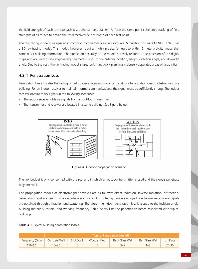
50
the field strength of each route to each test point can be obtained. Perform the same point coherence stacking of field
strengths of all routes to obtain the total received field strength of each test point.
The ray tracing model is integrated in common commercial planning software. Simulation software GENEX U-Net uses
a 3D ray tracing model. This model, however, requires highly precise (at least to within 5 meters) digital maps that
contain 3D building information. The prediction accuracy of the model is closely related to the precision of the digital
maps and accuracy of site engineering parameters, such as the antenna position, height, direction angle, and down-tilt
angle. Due to the cost, the ray tracing model is used only in network planning in densely populated areas of large cities.
4.2.4 Penetration Loss
Penetration loss indicates the fading of radio signals from an indoor terminal to a base station due to obstruction by a
building. For an indoor receiver to maintain normal communications, the signal must be sufficiently strong. The indoor
receiver obtains radio signals in the following scenarios:
The indoor receiver obtains signals from an outdoor transmitter. •
The transmitter and receiver are located in a same building. See Figure below •
The link budget is only concerned with the scenario in which an outdoor transmitter is used and the signals penetrate
only one wall.
The propagation modes of electromagnetic waves are as follows: direct radiation, inverse radiation, diffraction,
penetration, and scattering. In areas where no indoor distributed system is deployed, electromagnetic wave signals
are obtained through diffraction and scattering. Therefore, the indoor penetration loss is related to the incident angle,
building materials, terrain, and working frequency. Table below lists the penetration losses associated with typical
buildings.
Figure 4-3 Indoor propagation scenario
Table 4-3 Typical building penetration losses
Typical Penetration Loss (dB)
Frequency (GHz) Concrete Wall Brick Wall Wooden Floor Thick Glass Wall Thin Glass Wall Lift Door
1.8~2.6 15~30 10 5 3~5 1~3 20-30
51
In the link budget, penetration loss values depend on the coverage scenario. Therefore, coverage target areas are
classified into densely populated urban areas, common urban areas, suburban areas, rural areas, and highways. Table
below lists the area classification principles.
The building penetration loss ranges from 5 dB to 40 dB. In link budget, if no actual test data in the target area is
available, an assumed penetration loss value must be used. The final assumption is also highly dependent on local
customer requirement. For example in sophisticated Asian Metropolis like Hong Kong, Singapore and Shanghai, the
indoor coverage expectation will be very high, hence requiring a high penetration loss provisioning. On the other
hand, in less developed market such as Africa and Latin America, customer expectation is lower so the penetration loss
requirement can be reduced to reduce overall cost involved. During network planning, if no actual field testing data is
available, refer to the penetration loss values listed in Table below.
Table 4-4 Principles for classifying coverage scenarios
Scenario Name Description
Densely populated urban area
In this scenario, buildings are densely distributed, and the average building height exceeds 30 m. In certain areas, buildings are distributed in order. The distance between buildings is narrow and is not fixed. The average distance between buildings is 10 m to 20 m. Most streets that are not main avenues are narrow. These areas are densely populated.
Common urban areaIn this scenario, the average building height is about 20 m. The average distance between buildings is similar to the average building height. Such areas contain a certain amount of open spaces and greenery.
Suburban areaIn this scenario, the average building height is about 10 m. Buildings are scattered and the average distance between buildings is 30 to 50 m. The streets are wide. Such areas may contain much greenery and many open spaces.
Rural areaIn this scenario, buildings are scarce. The average building height is about 5 m. Such areas are likely to contain vast open spaces, fields, greenery, and roads.
Table 4-5 Example of penetration loss
Scenario Penetration Loss
Densely populated urban area 18 - 25 dB
Common urban area 15 - 18 dB
Suburban area 10 - 12 dB
Rural area 6 - 8 dB
4.2.5 Body Loss
Body loss indicates the loss generated due to signal blocking and absorption when a terminal antenna is close to the
body. This affects handsets in particular. Body loss depends on the position of the terminal. For fixed service, normally
USB dongle is used. Terminals, such as indoor and outdoor CPEs, are often mounted on roofs, windows, or desks. An
eNodeB antenna is mounted at a height of tens of meters, in which case body loss can be ignored as the body loss
value is 0 dB. For mobile applications, especially PDA-based VoIP services, body loss must be considered and in this
instance, the body loss is about 3 dB.
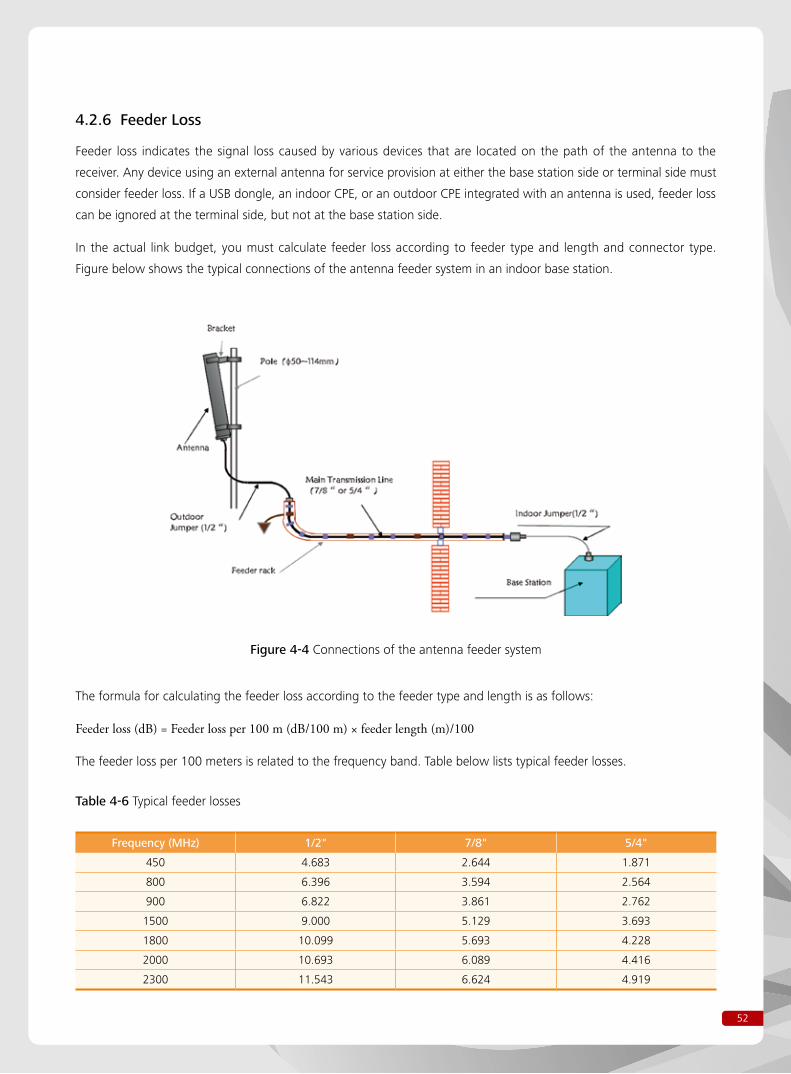
52
Table 4-6 Typical feeder losses
Frequency (MHz) 1/2" 7/8" 5/4"
450 4.683 2.644 1.871
800 6.396 3.594 2.564
900 6.822 3.861 2.762
1500 9.000 5.129 3.693
1800 10.099 5.693 4.228
2000 10.693 6.089 4.416
2300 11.543 6.624 4.919
4.2.6 Feeder Loss
Feeder loss indicates the signal loss caused by various devices that are located on the path of the antenna to the
receiver. Any device using an external antenna for service provision at either the base station side or terminal side must
consider feeder loss. If a USB dongle, an indoor CPE, or an outdoor CPE integrated with an antenna is used, feeder loss
can be ignored at the terminal side, but not at the base station side.
In the actual link budget, you must calculate feeder loss according to feeder type and length and connector type.
Figure below shows the typical connections of the antenna feeder system in an indoor base station.
The formula for calculating the feeder loss according to the feeder type and length is as follows:
Feeder loss (dB) = Feeder loss per 100 m (dB/100 m) × feeder length (m)/100
The feeder loss per 100 meters is related to the frequency band. Table below lists typical feeder losses.
Figure 4-4 Connections of the antenna feeder system
53
Frequency (MHz) 1/2" 7/8" 5/4"
2400 11.733 6.733 5.000
2500 12.035 6.906 5.129
3000 13.218 7.525 5.624
3300 13.932 7.932 5.928
3500 14.348 8.169 6.105
If a base station is mounted indoors, the link budget must include the losses of all devices from the RF port of the base
station to the antenna interface, including the indoor jumper, connector, main transmission feeder, combiners, splitters
and the outdoor jumper. If the RRU of a distributed base station is mounted on the tower top, you need to consider
only the loss of the outdoor 1/2" jumper. In this case, the total cable loss can be greatly reduced to approximately 0.5dB.
4.2.7 Background Noise
The background noise of the LTE system is the same as that of other communication systems. The calculation formula
is as follows:
Nth = KTB. K indicates the Boltzmann constant.
The value is as follows: 1.38 x 10 ^ (- 23)J/K. T indicates absolute temperature at a value of 290K. The result of KT is
the density of the heat noise power spectrum and the value is -174dBm/Hz. B indicates channel bandwidth and in LTE,
it can be 1.4MHz/3MHz/5 MHz/10 MHz/15 MHz/20 MHz
4.3 Equipment-Related Parameters
Equipment-related parameters include the base station, antenna, and terminal. The link budget parameters vary with
the base stations, antennas, and terminals of different vendors. These parameters affect the link budget result. As a
result, the downlink is unaffected in most scenarios.
4.3.1 Transmit Power
Transmit power includes that of the base station and terminal sides. The transmit power at the base station side affects
the downlink budget. The transmit power at the terminal side affects the uplink budget.
With the adoption of MIMO technology, two or more antennae are used at the same time at the base station for
transmission. Therefore, the power combining gain must be considered. The formula for calculating the power
combining gain is as follows:
Power Combining Gain=10*Log(N)
Where, N indicates the number of transmit channels of the base station.
For example, when a base station contains two transmitters and two receivers, the power combining gain is 3 dB.
Therefore, the transmit power in each sector (2T2R) is as follows:
46 dBm (40 Watt) in total for a 2x2 system with 20W from each transmit path
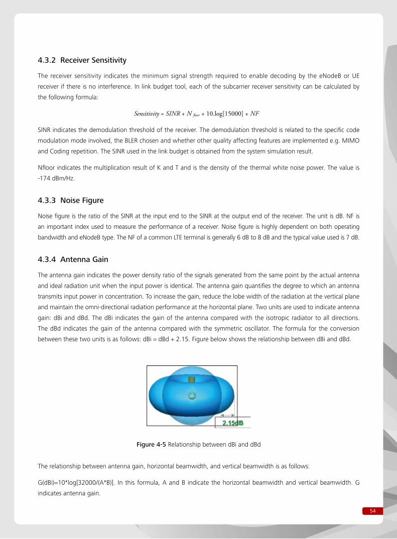
54
4.3.2 Receiver Sensitivity
The receiver sensitivity indicates the minimum signal strength required to enable decoding by the eNodeB or UE
receiver if there is no interference. In link budget tool, each of the subcarrier receiver sensitivity can be calculated by
the following formula:
Sensitivity = SINR + N floor + 10.log[15000] + NF
SINR indicates the demodulation threshold of the receiver. The demodulation threshold is related to the specific code
modulation mode involved, the BLER chosen and whether other quality affecting features are implemented e.g. MIMO
and Coding repetition. The SINR used in the link budget is obtained from the system simulation result.
Nfloor indicates the multiplication result of K and T and is the density of the thermal white noise power. The value is
-174 dBm/Hz.
4.3.3 Noise Figure
Noise figure is the ratio of the SINR at the input end to the SINR at the output end of the receiver. The unit is dB. NF is
an important index used to measure the performance of a receiver. Noise figure is highly dependent on both operating
bandwidth and eNodeB type. The NF of a common LTE terminal is generally 6 dB to 8 dB and the typical value used is 7 dB.
4.3.4 Antenna Gain
The antenna gain indicates the power density ratio of the signals generated from the same point by the actual antenna
and ideal radiation unit when the input power is identical. The antenna gain quantifies the degree to which an antenna
transmits input power in concentration. To increase the gain, reduce the lobe width of the radiation at the vertical plane
and maintain the omni-directional radiation performance at the horizontal plane. Two units are used to indicate antenna
gain: dBi and dBd. The dBi indicates the gain of the antenna compared with the isotropic radiator to all directions.
The dBd indicates the gain of the antenna compared with the symmetric oscillator. The formula for the conversion
between these two units is as follows: dBi = dBd + 2.15. Figure below shows the relationship between dBi and dBd.
Figure 4-5 Relationship between dBi and dBd
The relationship between antenna gain, horizontal beamwidth, and vertical beamwidth is as follows:
G(dBi)=10*log[32000/(A*B)]. In this formula, A and B indicate the horizontal beamwidth and vertical beamwidth. G
indicates antenna gain.
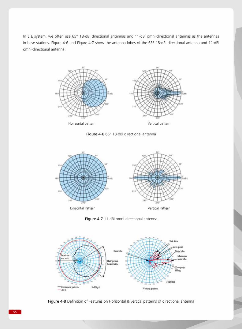
55
In LTE system, we often use 65° 18-dBi directional antennas and 11-dBi omni-directional antennas as the antennas
in base stations. Figure 4-6 and Figure 4-7 show the antenna lobes of the 65° 18-dBi directional antenna and 11-dBi
omni-directional antenna.
Horizontal pattern Vertical pattern
Figure 4-6 65° 18-dBi directional antenna
Horizontal Pattern Vertical Pattern
Figure 4-7 11-dBi omni-directional antenna
Figure 4-8 Definition of Features on Horizontal & vertical patterns of directional antenna
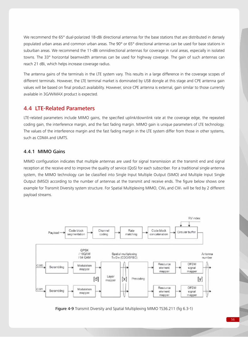
56
We recommend the 65° dual-polarized 18-dBi directional antennas for the base stations that are distributed in densely
populated urban areas and common urban areas. The 90° or 65° directional antennas can be used for base stations in
suburban areas. We recommend the 11-dBi omnidirectional antennas for coverage in rural areas, especially in isolated
towns. The 33° horizontal beamwidth antennas can be used for highway coverage. The gain of such antennas can
reach 21 dBi, which helps increase coverage radius.
The antenna gains of the terminals in the LTE system vary. This results in a large difference in the coverage scopes of
different terminals. However, the LTE terminal market is dominated by USB dongle at this stage and CPE antenna gain
values will be based on final product availability. However, since CPE antenna is external, gain similar to those currently
available in 3G/WiMAX product is expected.
4.4 LTE-Related Parameters
LTE-related parameters include MIMO gains, the specified uplink/downlink rate at the coverage edge, the repeated
coding gain, the interference margin, and the fast fading margin. MIMO gain is unique parameters of LTE technology.
The values of the interference margin and the fast fading margin in the LTE system differ from those in other systems,
such as CDMA and UMTS.
4.4.1 MIMO Gains
MIMO configuration indicates that multiple antennas are used for signal transmission at the transmit end and signal
reception at the receive end to improve the quality of service (QoS) for each subscriber. For a traditional single-antenna
system, the MIMO technology can be classified into Single Input Multiple Output (SIMO) and Multiple Input Single
Output (MISO) according to the number of antennas at the transmit and receive ends. The figure below shows one
example for Transmit Diversity system structure. For Spatial Multiplexing MIMO, CW0 and CW1 will be fed by 2 different
payload streams.
Figure 4-9 Transmit Diversity and Spatial Multiplexing MIMO TS36.211 (fig 6.3-1)
57
In the example above, a single data input stream is used to feed two separate antennae but it is equally possible to
feed two different input data streams into this setup to provide higher data rate and it is the fundamental principle for
Multiple Code Word (MCW) in LTE.
Multi-antenna technology can improve system capacity and coverage without largely increasing cost. This is because
the multi-antenna technology gives the following gains: power combining gain, array gain, space diversity gain,
and interference reduction gain. In addition, the MIMO achieves a spatial multiplexing gain, which is mainly used to
increase the system capacity. This section describes the various gains brought by the MIMO.
1. Power combining gain
When multiple antennae (N) are used to transmit signals, N transmit channels are available. In this case, the total
transmit power is equal to N times the transmit power from a single antenna signal transmission. As a result, a
power gain of 10log(N) dB can be obtained. If a single antenna is used to transmit signals, you can also increase the
transmit power. In this case, however, the requirements for the power amplifier are high, and implementation cost
is complex and increased.
2. Array gain
The array gain indicates an improvement in the average signal noise ratio (SINR) at the receive end when the total
transmit power is the same. The array gain can be obtained through the coherent combining of various antenna
signals. Various multi-antenna systems can obtain the array gain. That is, after the multi-antenna technology is used,
the receiving SINR can be improved.
3. Space diversity gain
Due to the fading nature of wireless channels, the signals in a single-antenna system suffer from deep fading. In
a multi-antenna system, the distance between antennae is often large. This ensures that the signal fading of an
antenna is independent. Therefore, the SINR fluctuation of the received signals after combining stabilizes, thus
improving received signal quality.
4. Interference reduction gain
In mobile cellular communications system, inter-cell interference cannot be ignored due to the frequency sharing
and multiplexing nature both within and between cells. However, different from white noise, the interference signal
is colored noise. You can combine the expected signals and suppress the interference signal through proper multi-
antenna spatial weight at the receiving end to improve the average SINR at the receiving end. This is the basis of
Interference Reduction Combining feature.
5. Spatial multiplexing gain
The spatial multiplexing gain indicates the improvement of data throughput or transmission rate when the transmit
power and bandwidth remain unchanged. You can obtain a spatial multiplexing gain by transmitting multiple
parallel data streams over the same time-frequency resources. The spatial multiplexing gain is used to increase
system capacity.
4.4.2 Cell Edge Rate
Similar to other wireless communications systems, such as CDMA2000 EVDO, WiMAX and HSPA, the LTE features a
rate layering feature. That is, the higher the required edge rate, the smaller the cell coverage radius. The lower the
58
required edge rate, the larger the cell coverage radius. This comes about due to the fixed power offered by UE (normally
23dBm) being spread evenly to the number of RBs involved in the modulation scheme assigned, assuming there is no
power control (i.e. Downlink ICIC also disabled). Some of the factors that affect the edge rate in the LTE system are as
follows:
Uplink/downlink TDD proportion •
MIMO schemes chosen •
eNodeB Power Amplifier power (affect downlink only) •
Number of RB used at the sector edge •
Modulation mode (1 of 29 coding methods) •
Repeated coding times •
The formula for calculating the downlink cell edge rate is as follows:
Cell edge rate_Phy = Number of Different data stream transmitted x Number of Resource Block assigned to
user per frame x Number of available Traffic carrying Resource Element per Resource Block x Coding rate x
Modulation model level / Duration of each frame - Where,
Number of Resource Block Assigned (a single RB is the basic resource assignment level) reflects the number of
resource blocks used by user at the edge of the sector. The smaller the number of resource blocks assigned, the
lower the cell edge rate. In previous version of link budget tools, receive sensitivity of a base station is defined by the
bandwidth of the RB which is 180 kHz. More recent version are using per subcarrier as basis of receiver sensitivity and
the conversion value is simply 10log10(12). RB can be assigned down to a per TTI level (1 ms duration)
Number of Different data stream transmitted is related to the number of data stream being simultaneously
transmitted. Number can be ranging from 1 (SFBC) to 2 (MCW 2x2). In case of BF, the value should be 1 for single
antenna port transmission mode 7 (port 7 or 8), and 2 streams for dual antenna port transmission mode 8 (port 7 and 8).
Number of available Traffic carrying Resource Element per Resource Block indicates the number of RE available
for each resource block. In FDD system, a maximum of 3 symbols (36 Res) can be consumed per frame (10ms) for
control channel signaling purposes and there is at least 6 more extra RE can be used for Downlink Reference signaling
per TTI (1ms). A minimum of 1 symbol (12 Res) will be required per RB for control signaling purposes. In TDD system,
due to frequency sharing and time gap requirement for switching between uplink and downlink, 6 symbols equivalent
(72 Res) will be the minimum overhead requirement per TTI.
Coding rate indicates the volume coding rate of the channel code. For example, the volume coding rate of QPSK1/2 is
1/2, and the volume coding rate of 16QAM3/4 is 3/4.
Modulation model level indicates the number of bits in the modulation mode. For example, the modulation mode
levels of QPSK, 16QAM, and 64QAM are 2, 4, and 6 respectively.
Duration of each frame indicates the frame size. As regulated by the protocols, the frame size in LTE networks is 10 ms.
In the link budget, the settings of the uplink/downlink cell edge rates (in particular the uplink cell edge rate) will
determine the final cell coverage radius. Hence, an understanding of edge coverage requirement is very critical from
a network planning perspective. If Downlink ICIC is enabled, downlink power control must be enabled also (which
is executed at 20ms intervals based on UE BER reported value) and edge rate calculation will be more complex and
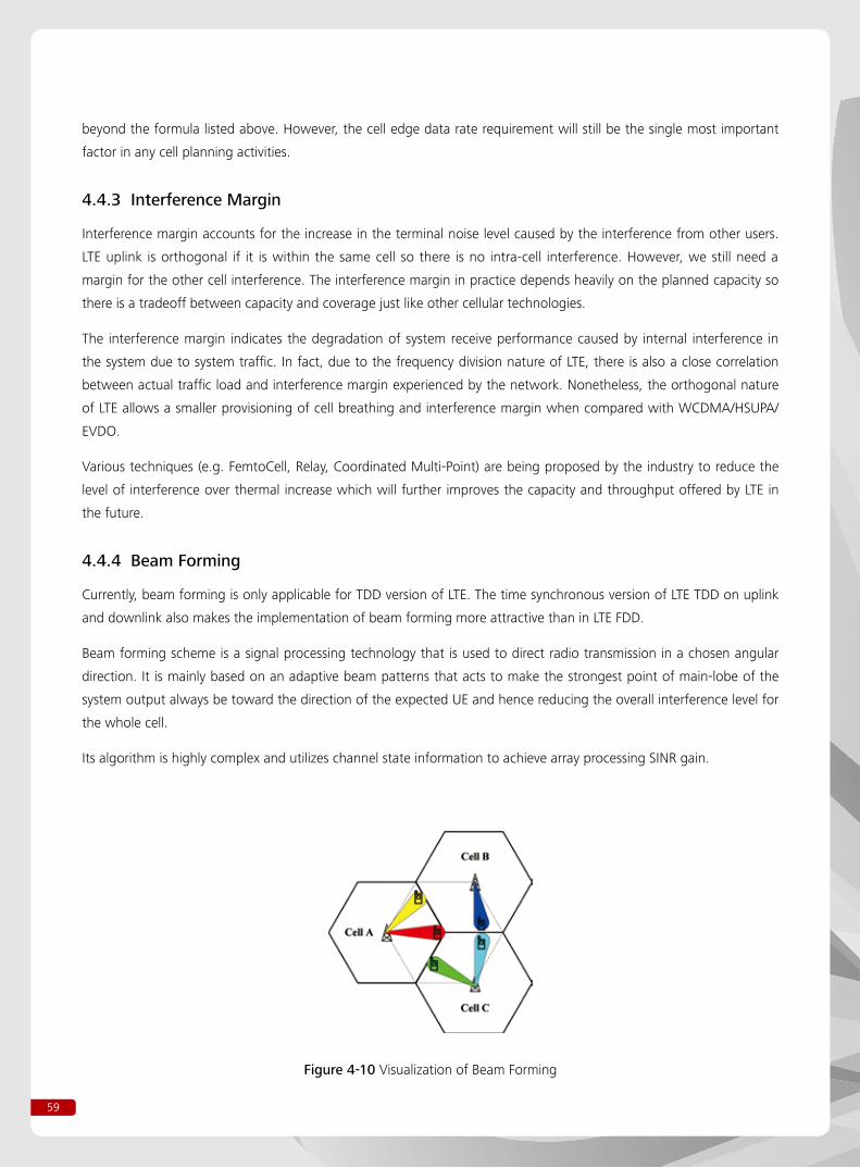
59
beyond the formula listed above. However, the cell edge data rate requirement will still be the single most important
factor in any cell planning activities.
4.4.3 Interference Margin
Interference margin accounts for the increase in the terminal noise level caused by the interference from other users.
LTE uplink is orthogonal if it is within the same cell so there is no intra-cell interference. However, we still need a
margin for the other cell interference. The interference margin in practice depends heavily on the planned capacity so
there is a tradeoff between capacity and coverage just like other cellular technologies.
The interference margin indicates the degradation of system receive performance caused by internal interference in
the system due to system traffic. In fact, due to the frequency division nature of LTE, there is also a close correlation
between actual traffic load and interference margin experienced by the network. Nonetheless, the orthogonal nature
of LTE allows a smaller provisioning of cell breathing and interference margin when compared with WCDMA/HSUPA/
EVDO.
Various techniques (e.g. FemtoCell, Relay, Coordinated Multi-Point) are being proposed by the industry to reduce the
level of interference over thermal increase which will further improves the capacity and throughput offered by LTE in
the future.
4.4.4 Beam Forming
Currently, beam forming is only applicable for TDD version of LTE. The time synchronous version of LTE TDD on uplink
and downlink also makes the implementation of beam forming more attractive than in LTE FDD.
Beam forming scheme is a signal processing technology that is used to direct radio transmission in a chosen angular
direction. It is mainly based on an adaptive beam patterns that acts to make the strongest point of main-lobe of the
system output always be toward the direction of the expected UE and hence reducing the overall interference level for
the whole cell.
Its algorithm is highly complex and utilizes channel state information to achieve array processing SINR gain.
Figure 4-10 Visualization of Beam Forming
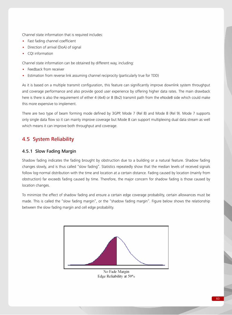
60
Channel state information that is required includes:
Fast fading channel coefficient •
Direction of arrival (DoA) of signal •
CQI information •
Channel state information can be obtained by different way, including:
Feedback from receiver •
Estimation from reverse link assuming channel reciprocity (particularly true for TDD) •
As it is based on a multiple transmit configuration, this feature can significantly improve downlink system throughput
and coverage performance and also provide good user experience by offering higher data rates. The main drawback
here is there is also the requirement of either 4 (4x4) or 8 (8x2) transmit path from the eNodeB side which could make
this more expensive to implement.
There are two type of beam forming mode defined by 3GPP, Mode 7 (Rel 8) and Mode 8 (Rel 9). Mode 7 supports
only single data flow so it can mainly improve coverage but Mode 8 can support multiplexing dual data stream as well
which means it can improve both throughput and coverage.
4.5 System Reliability
4.5.1 Slow Fading Margin
Shadow fading indicates the fading brought by obstruction due to a building or a natural feature. Shadow fading
changes slowly, and is thus called “slow fading”. Statistics repeatedly show that the median levels of received signals
follow log-normal distribution with the time and location at a certain distance. Fading caused by location (mainly from
obstruction) far exceeds fading caused by time. Therefore, the major concern for shadow fading is those caused by
location changes.
To minimize the effect of shadow fading and ensure a certain edge coverage probability, certain allowances must be
made. This is called the “slow fading margin”, or the “shadow fading margin”. Figure below shows the relationship
between the slow fading margin and cell edge probability.
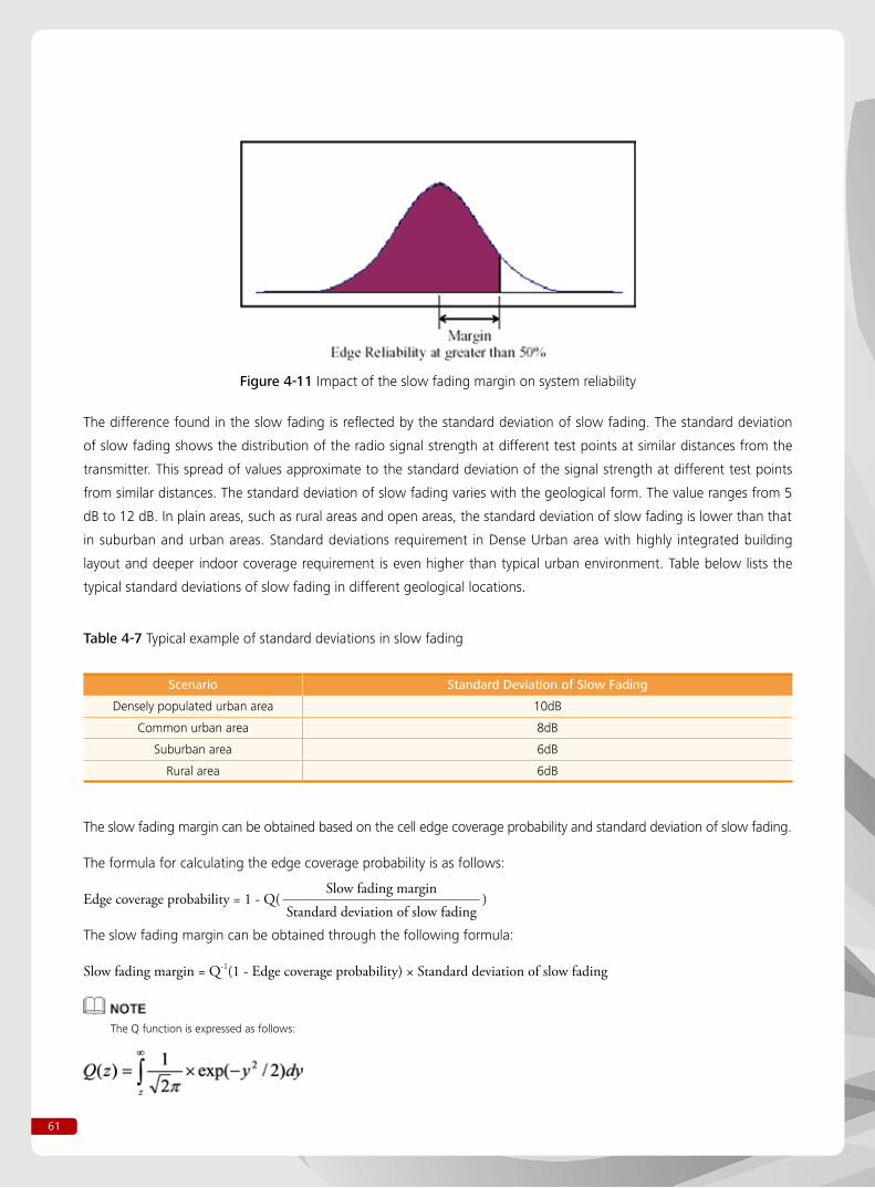
61
The difference found in the slow fading is reflected by the standard deviation of slow fading. The standard deviation
of slow fading shows the distribution of the radio signal strength at different test points at similar distances from the
transmitter. This spread of values approximate to the standard deviation of the signal strength at different test points
from similar distances. The standard deviation of slow fading varies with the geological form. The value ranges from 5
dB to 12 dB. In plain areas, such as rural areas and open areas, the standard deviation of slow fading is lower than that
in suburban and urban areas. Standard deviations requirement in Dense Urban area with highly integrated building
layout and deeper indoor coverage requirement is even higher than typical urban environment. Table below lists the
typical standard deviations of slow fading in different geological locations.
Table 4-7 Typical example of standard deviations in slow fading
Scenario Standard Deviation of Slow Fading
Densely populated urban area 10dB
Common urban area 8dB
Suburban area 6dB
Rural area 6dB
The slow fading margin can be obtained based on the cell edge coverage probability and standard deviation of slow fading.
The formula for calculating the edge coverage probability is as follows:
Edge coverage probability = 1 - Q( )
The slow fading margin can be obtained through the following formula:
Slow fading margin = Q-1(1 - Edge coverage probability) × Standard deviation of slow fading
Slow fading margin
Standard deviation of slow fading
The Q function is expressed as follows:
Figure 4-11 Impact of the slow fading margin on system reliability
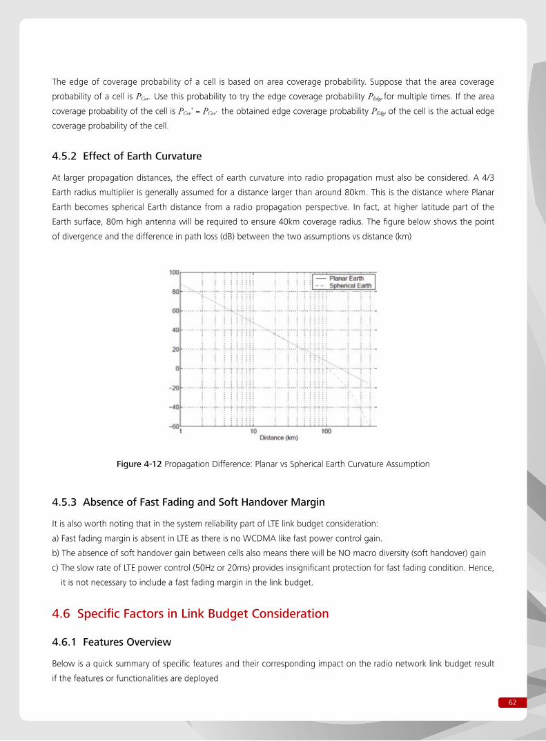
62
The edge of coverage probability of a cell is based on area coverage probability. Suppose that the area coverage
probability of a cell is PCov. Use this probability to try the edge coverage probability PEdge for multiple times. If the area
coverage probability of the cell is PCov' = PCov’ the obtained edge coverage probability PEdge of the cell is the actual edge
coverage probability of the cell.
4.5.2 Effect of Earth Curvature
At larger propagation distances, the effect of earth curvature into radio propagation must also be considered. A 4/3
Earth radius multiplier is generally assumed for a distance larger than around 80km. This is the distance where Planar
Earth becomes spherical Earth distance from a radio propagation perspective. In fact, at higher latitude part of the
Earth surface, 80m high antenna will be required to ensure 40km coverage radius. The figure below shows the point
of divergence and the difference in path loss (dB) between the two assumptions vs distance (km)
Figure 4-12 Propagation Difference: Planar vs Spherical Earth Curvature Assumption
4.5.3 Absence of Fast Fading and Soft Handover Margin
It is also worth noting that in the system reliability part of LTE link budget consideration:
a) Fast fading margin is absent in LTE as there is no WCDMA like fast power control gain.
b) The absence of soft handover gain between cells also means there will be NO macro diversity (soft handover) gain
c) The slow rate of LTE power control (50Hz or 20ms) provides insignificant protection for fast fading condition. Hence,
it is not necessary to include a fast fading margin in the link budget.
4.6 Specific Factors in Link Budget Consideration
4.6.1 Features Overview
Below is a quick summary of specific features and their corresponding impact on the radio network link budget result
if the features or functionalities are deployed
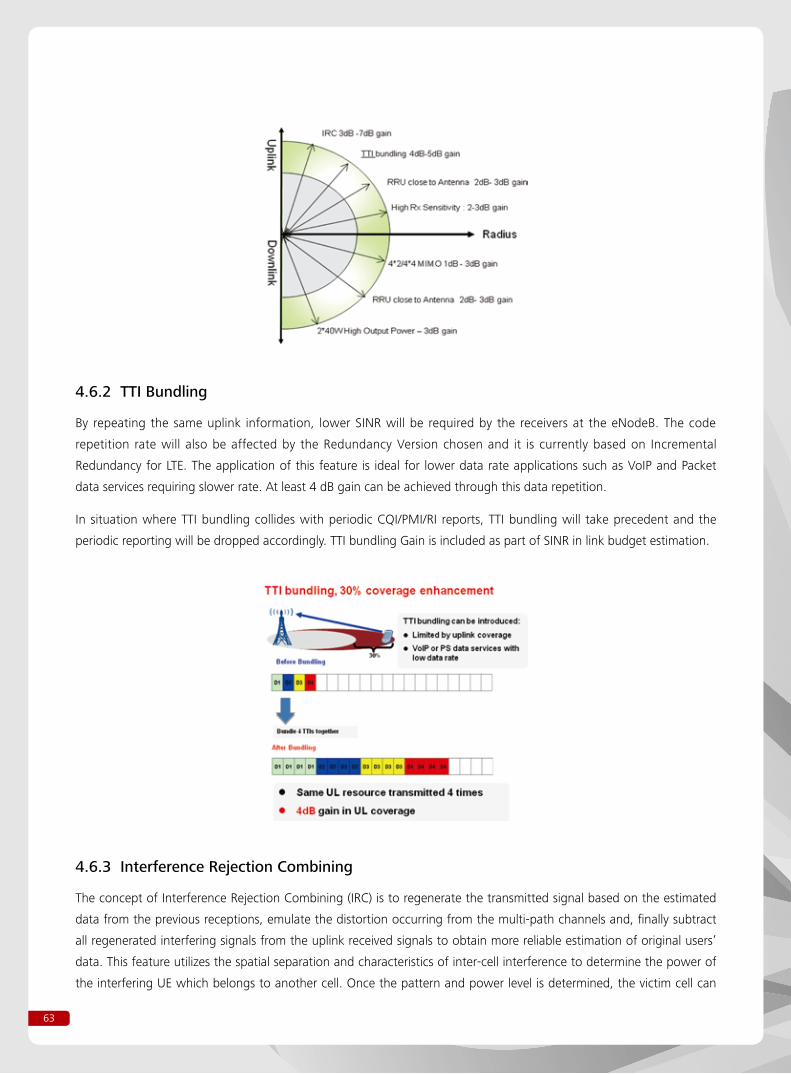
63
4.6.2 TTI Bundling
By repeating the same uplink information, lower SINR will be required by the receivers at the eNodeB. The code
repetition rate will also be affected by the Redundancy Version chosen and it is currently based on Incremental
Redundancy for LTE. The application of this feature is ideal for lower data rate applications such as VoIP and Packet
data services requiring slower rate. At least 4 dB gain can be achieved through this data repetition.
In situation where TTI bundling collides with periodic CQI/PMI/RI reports, TTI bundling will take precedent and the
periodic reporting will be dropped accordingly. TTI bundling Gain is included as part of SINR in link budget estimation.
4.6.3 Interference Rejection Combining
The concept of Interference Rejection Combining (IRC) is to regenerate the transmitted signal based on the estimated
data from the previous receptions, emulate the distortion occurring from the multi-path channels and, finally subtract
all regenerated interfering signals from the uplink received signals to obtain more reliable estimation of original users’
data. This feature utilizes the spatial separation and characteristics of inter-cell interference to determine the power of
the interfering UE which belongs to another cell. Once the pattern and power level is determined, the victim cell can
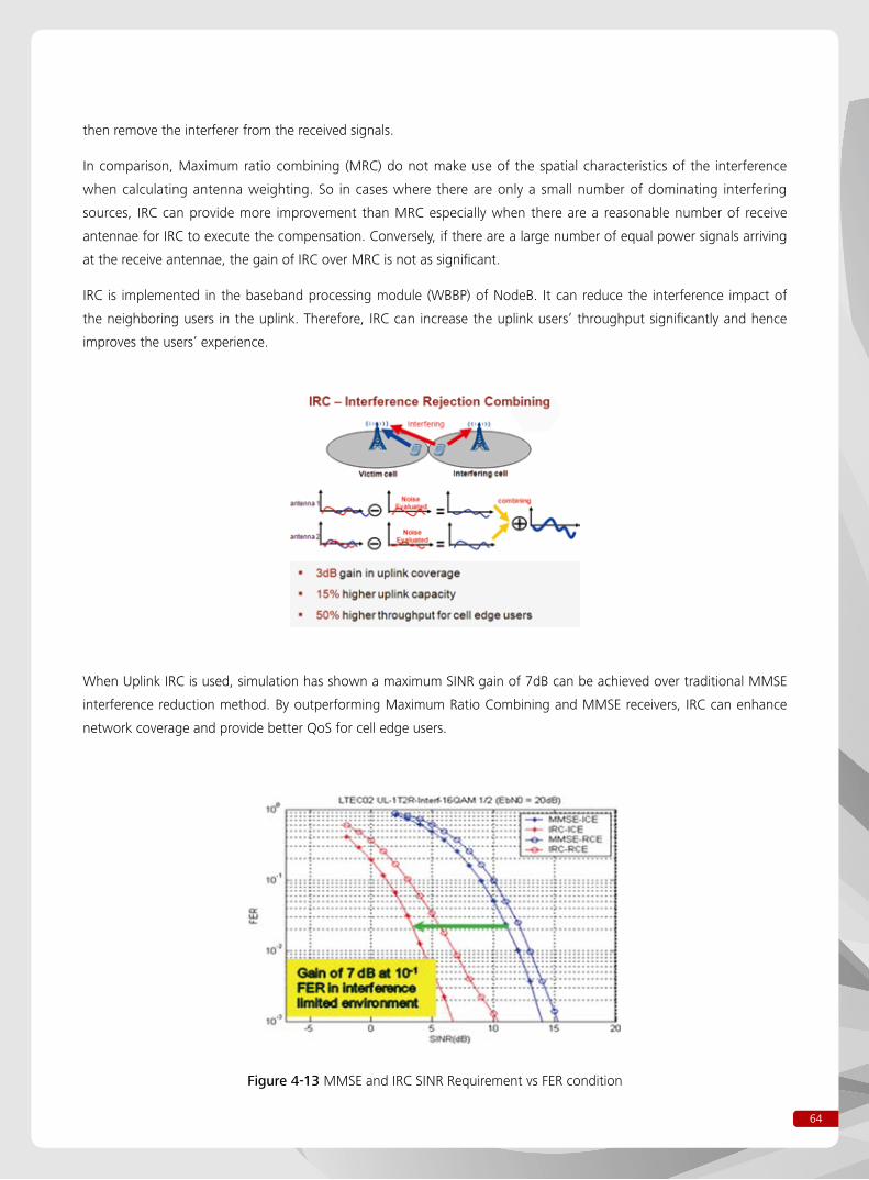
64
then remove the interferer from the received signals.
In comparison, Maximum ratio combining (MRC) do not make use of the spatial characteristics of the interference
when calculating antenna weighting. So in cases where there are only a small number of dominating interfering
sources, IRC can provide more improvement than MRC especially when there are a reasonable number of receive
antennae for IRC to execute the compensation. Conversely, if there are a large number of equal power signals arriving
at the receive antennae, the gain of IRC over MRC is not as significant.
IRC is implemented in the baseband processing module (WBBP) of NodeB. It can reduce the interference impact of
the neighboring users in the uplink. Therefore, IRC can increase the uplink users’ throughput significantly and hence
improves the users’ experience.
When Uplink IRC is used, simulation has shown a maximum SINR gain of 7dB can be achieved over traditional MMSE
interference reduction method. By outperforming Maximum Ratio Combining and MMSE receivers, IRC can enhance
network coverage and provide better QoS for cell edge users.
Figure 4-13 MMSE and IRC SINR Requirement vs FER condition
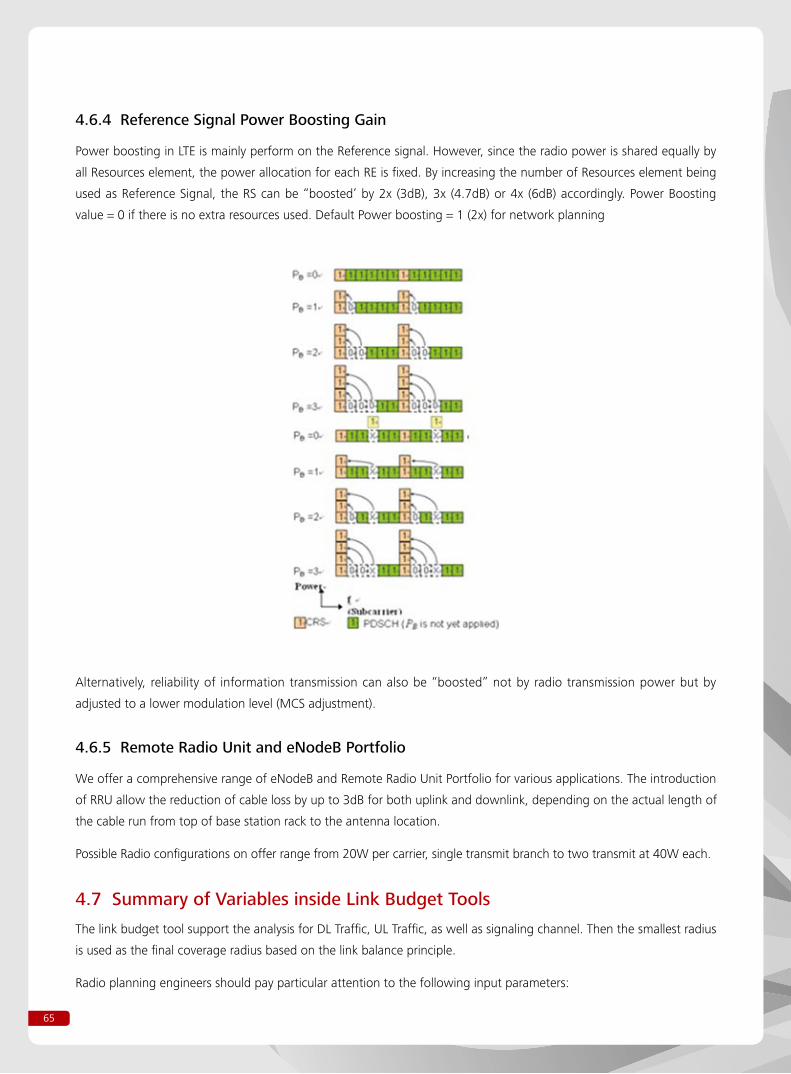
65
4.6.4 Reference Signal Power Boosting Gain
Power boosting in LTE is mainly perform on the Reference signal. However, since the radio power is shared equally by
all Resources element, the power allocation for each RE is fixed. By increasing the number of Resources element being
used as Reference Signal, the RS can be “boosted’ by 2x (3dB), 3x (4.7dB) or 4x (6dB) accordingly. Power Boosting
value = 0 if there is no extra resources used. Default Power boosting = 1 (2x) for network planning
Alternatively, reliability of information transmission can also be “boosted” not by radio transmission power but by
adjusted to a lower modulation level (MCS adjustment).
4.6.5 Remote Radio Unit and eNodeB Portfolio
We offer a comprehensive range of eNodeB and Remote Radio Unit Portfolio for various applications. The introduction
of RRU allow the reduction of cable loss by up to 3dB for both uplink and downlink, depending on the actual length of
the cable run from top of base station rack to the antenna location.
Possible Radio configurations on offer range from 20W per carrier, single transmit branch to two transmit at 40W each.
4.7 Summary of Variables inside Link Budget Tools
The link budget tool support the analysis for DL Traffic, UL Traffic, as well as signaling channel. Then the smallest radius
is used as the final coverage radius based on the link balance principle.
Radio planning engineers should pay particular attention to the following input parameters:
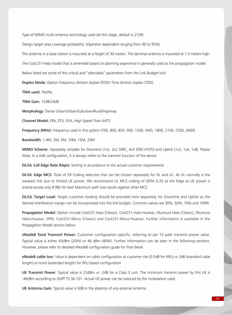
66
Type of MIMO multi-antenna technology used (At this stage, default is 2T2R)
Design target area coverage probability. (Operator dependent ranging from 90 to 95%)
The antenna in a base station is mounted at a height of 30 meters. The terminal antenna is mounted at 1.5 meters high.
The Cost231-Hata model that is amended based on planning experience is generally used as the propagation model.
Below listed are some of the critical and “selectable” parameters from the Link Budget tool
Duplex Mode: Option Frequency division duplex (FDD)/ Time division duplex (TDD).
TMA used: Yes/No
TMA Gain: 12dB/24dB
Morphology: Dense Urban/Urban/Suburban/Rural/Highway
Channel Model: EPA, ETU, EVA, High Speed Train (HST)
Frequency (MHz): Frequency used in this system (700, 800, 850, 900, 1500, AWS, 1800, 2100, 2300, 2600)
Bandwidth: 1.4M, 3M, 5M, 10M, 15M, 20M
MIMO Scheme: Separately settable for Downlink (1x2, 2x2 SFBC, 4x2 SFBC+FSTD) and Uplink (1x2, 1x4, 1x8). Please
Note, In a AxB configuration, A is always refers to the transmit function of the device
DL/UL Cell Edge Rate (kbps): Setting in accordance to the actual customer requirements
DL/UL Edge MCS: Total of 29 Coding selection that can be chosen separately for DL and UL. As UL normally is the
weakest link due to limited UE power, We recommend UL MCS coding of QPSK 0.25 at the Edge as UE power is
shared across only 8 RBs for best Maximum path loss results against other MCS.
DL/UL Target Load: Target customer loading should be provided here separately for Downlink and Uplink so the
desired interference margin can be incorporated into the link budget. Common values are 30%, 50%, 70% and 100%
Propagation Model: Option include Cost231-Hata (Classic), Cost231-Hata-Huawei, Okumura Hata (Classic), Okumura
Hata-Huawei, SPM, Cost231-Micro (Classic) and Cost231-Micro-Huawei. Further information is available in the
Propagation Model section below
eNodeB Total Transmit Power: Customer configuration specific, referring to per TX path transmit power value.
Typical value is either 43dBm (20W) or 46 dBm (40W). Further information can be seen in the following sections.
However, please refer to detailed eNodeB configuration guide for final detail.
eNodeB cable loss: Value is dependent on cable configuration at customer site (0.5dB for RRU) vs 3dB (standard cable
length) or more (extended length) for RFU based configuration
UE Transmit Power: Typical value is 23dBm +/- 2dB for a Class 3 unit. The minimum transmit power by this UE is
-40dBm according to 3GPP TS 36.101. Actual UE power can be reduced by the modulation used.
UE Antenna Gain: Typical value is 0dB in the absence of any external antenna
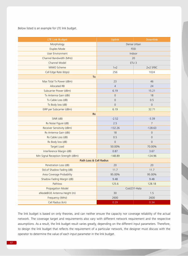
67
Below listed is an example for LTE link budget.
LTE Link Budget Uplink Downlink
Morphology Dense Urban
Duplex Mode FDD
User Environment Indoor
Channel Bandwidth (MHz) 20
Channel Model ETU 3
MIMO Scheme 1×2 2×2 SFBC
Cell Edge Rate (kbps) 256 1024
Tx
Max Total Tx Power (dBm) 23 46
Allocated RB 4 24
Subcarrier Power (dBm) 6.19 15.21
Tx Antenna Gain (dBi) 0 18
Tx Cable Loss (dB) 0 0.5
Tx Body loss (dB) 0 0
EIRP per Subcarrier (dBm) 6.19 32.71
Rx
SINR (dB) -2.52 -3.39
Rx Noise Figure (dB) 2.5 7
Receiver Sensitivity (dBm) -132.26 -128.63
Rx Antenna Gain (dBi) 18 0
Rx Cable Loss (dB) 0.5 0
Rx Body loss (dB) 0 0
Target Load 50.00% 70.00%
Interference Margin (dB) 0.87 3.67
Min Signal Reception Strength (dBm) -148.89 -124.96
Path Loss & Cell Radius
Penetration Loss (dB) 20 20
Std.of Shadow Fading (dB) 11.7 11.7
Area Coverage Probability 95.00% 95.00%
Shadow Fading Margin (dB) 9.48 9.48
Pathloss 125.6 128.18
Propagation Model Cost231-Hata
eNodeB/UE Antenna Height (m) 30 1.5
Frequency (MHz) 2600 2600
Cell Radius (km) 0.29 0.34
The link budget is based on only theories, and can neither ensure the capacity nor coverage reliability of the actual
network. The coverage target and requirements also vary with different network requirement and the respective
assumptions. As a result, the link budget result varies greatly, depending on the different input parameters. Therefore,
to design the link budget that reflects the requirement of a particular network, the designer must discuss with the
operator to determine the value of each input parameter in the link budget.

68
Link budget also assumes a uniform landform, simple terrain, ideal site locations, and even subscriber distribution.
System simulation covers detailed landform distribution, actual site location, terrain type, and subscriber distribution.
Hence, the link budget result serves ONLY as the theoretical calculation result. The calculated coverage radius is
used for reference in simulated site distribution. The detailed coverage planning must be completed through system
simulation. For a given coverage area, the number of planned base stations will depend on the system simulation
result.
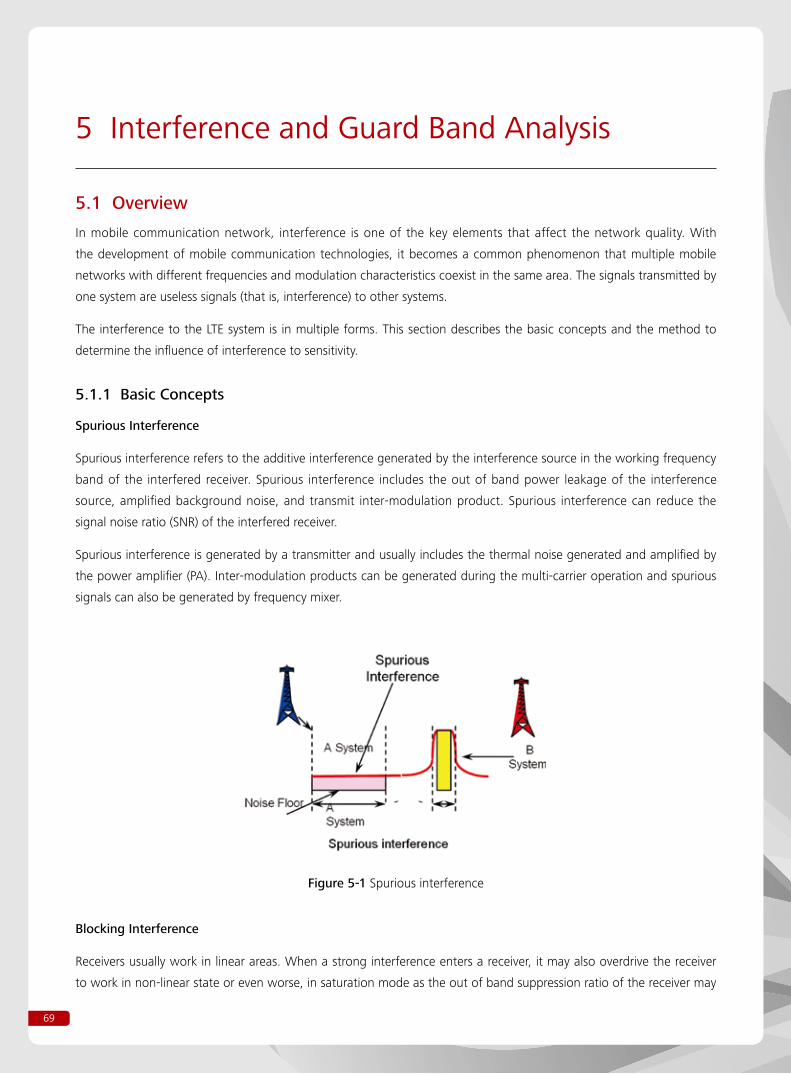
69
5 Interference and Guard Band Analysis
5.1 Overview
In mobile communication network, interference is one of the key elements that affect the network quality. With
the development of mobile communication technologies, it becomes a common phenomenon that multiple mobile
networks with different frequencies and modulation characteristics coexist in the same area. The signals transmitted by
one system are useless signals (that is, interference) to other systems.
The interference to the LTE system is in multiple forms. This section describes the basic concepts and the method to
determine the influence of interference to sensitivity.
5.1.1 Basic Concepts
Spurious Interference
Spurious interference refers to the additive interference generated by the interference source in the working frequency
band of the interfered receiver. Spurious interference includes the out of band power leakage of the interference
source, amplified background noise, and transmit inter-modulation product. Spurious interference can reduce the
signal noise ratio (SNR) of the interfered receiver.
Spurious interference is generated by a transmitter and usually includes the thermal noise generated and amplified by
the power amplifier (PA). Inter-modulation products can be generated during the multi-carrier operation and spurious
signals can also be generated by frequency mixer.
Blocking Interference
Receivers usually work in linear areas. When a strong interference enters a receiver, it may also overdrive the receiver
to work in non-linear state or even worse, in saturation mode as the out of band suppression ratio of the receiver may
Figure 5-1 Spurious interference
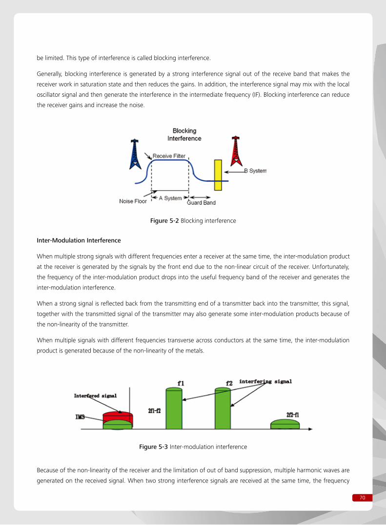
70
Figure 5-2 Blocking interference
be limited. This type of interference is called blocking interference.
Generally, blocking interference is generated by a strong interference signal out of the receive band that makes the
receiver work in saturation state and then reduces the gains. In addition, the interference signal may mix with the local
oscillator signal and then generate the interference in the intermediate frequency (IF). Blocking interference can reduce
the receiver gains and increase the noise.
Inter-Modulation Interference
When multiple strong signals with different frequencies enter a receiver at the same time, the inter-modulation product
at the receiver is generated by the signals by the front end due to the non-linear circuit of the receiver. Unfortunately,
the frequency of the inter-modulation product drops into the useful frequency band of the receiver and generates the
inter-modulation interference.
When a strong signal is reflected back from the transmitting end of a transmitter back into the transmitter, this signal,
together with the transmitted signal of the transmitter may also generate some inter-modulation products because of
the non-linearity of the transmitter.
When multiple signals with different frequencies transverse across conductors at the same time, the inter-modulation
product is generated because of the non-linearity of the metals.
Figure 5-3 Inter-modulation interference
Because of the non-linearity of the receiver and the limitation of out of band suppression, multiple harmonic waves are
generated on the received signal. When two strong interference signals are received at the same time, the frequency
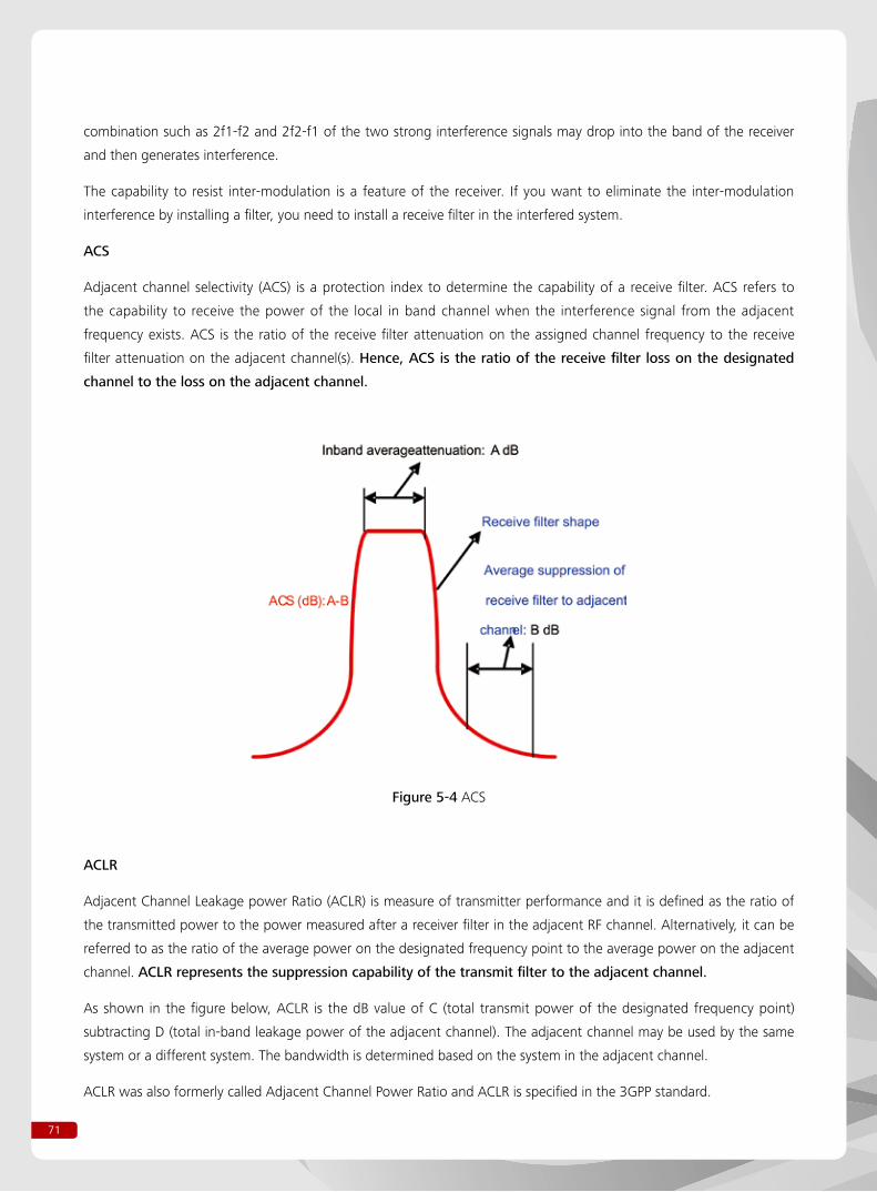
71
combination such as 2f1-f2 and 2f2-f1 of the two strong interference signals may drop into the band of the receiver
and then generates interference.
The capability to resist inter-modulation is a feature of the receiver. If you want to eliminate the inter-modulation
interference by installing a filter, you need to install a receive filter in the interfered system.
ACS
Adjacent channel selectivity (ACS) is a protection index to determine the capability of a receive filter. ACS refers to
the capability to receive the power of the local in band channel when the interference signal from the adjacent
frequency exists. ACS is the ratio of the receive filter attenuation on the assigned channel frequency to the receive
filter attenuation on the adjacent channel(s). Hence, ACS is the ratio of the receive filter loss on the designated
channel to the loss on the adjacent channel.
Figure 5-4 ACS
ACLR
Adjacent Channel Leakage power Ratio (ACLR) is measure of transmitter performance and it is defined as the ratio of
the transmitted power to the power measured after a receiver filter in the adjacent RF channel. Alternatively, it can be
referred to as the ratio of the average power on the designated frequency point to the average power on the adjacent
channel. ACLR represents the suppression capability of the transmit filter to the adjacent channel.
As shown in the figure below, ACLR is the dB value of C (total transmit power of the designated frequency point)
subtracting D (total in-band leakage power of the adjacent channel). The adjacent channel may be used by the same
system or a different system. The bandwidth is determined based on the system in the adjacent channel.
ACLR was also formerly called Adjacent Channel Power Ratio and ACLR is specified in the 3GPP standard.
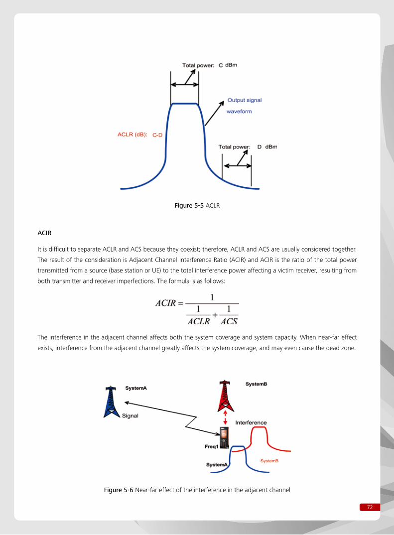
72
Figure 5-5 ACLR
Figure 5-6 Near-far effect of the interference in the adjacent channel
ACIR
It is difficult to separate ACLR and ACS because they coexist; therefore, ACLR and ACS are usually considered together.
The result of the consideration is Adjacent Channel Interference Ratio (ACIR) and ACIR is the ratio of the total power
transmitted from a source (base station or UE) to the total interference power affecting a victim receiver, resulting from
both transmitter and receiver imperfections. The formula is as follows:
The interference in the adjacent channel affects both the system coverage and system capacity. When near-far effect
exists, interference from the adjacent channel greatly affects the system coverage, and may even cause the dead zone.
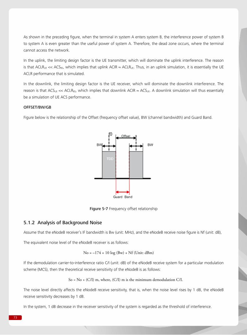
73
As shown in the preceding figure, when the terminal in system A enters system B, the interference power of system B
to system A is even greater than the useful power of system A. Therefore, the dead zone occurs, where the terminal
cannot access the network.
In the uplink, the limiting design factor is the UE transmitter, which will dominate the uplink interference. The reason
is that ACLRUE << ACSBS, which implies that uplink ACIR ≈ ACLRUE. Thus, in an uplink simulation, it is essentially the UE
ACLR performance that is simulated.
In the downlink, the limiting design factor is the UE receiver, which will dominate the downlink interference. The
reason is that ACSUE << ACLRBS, which implies that downlink ACIR ≈ ACSUE. A downlink simulation will thus essentially
be a simulation of UE ACS performance.
OFFSET/BW/GB
Figure below is the relationship of the Offset (frequency offset value), BW (channel bandwidth) and Guard Band.
Figure 5-7 Frequency offset relationship
5.1.2 Analysis of Background Noise
Assume that the eNodeB receiver’s IF bandwidth is Bw (unit: MHz), and the eNodeB receive noise figure is Nf (unit: dB),
The equivalent noise level of the eNodeB receiver is as follows:
No = –174 + 10 log (Bw) + Nf (Unit: dBm)
If the demodulation carrier-to-interference ratio C/I (unit: dB) of the eNodeB receive system for a particular modulation
scheme (MCS), then the theoretical receive sensitivity of the eNodeB is as follows:
So = No + (C/I) m, where, (C/I) m is the minimum demodulation C/I.
The noise level directly affects the eNodeB receive sensitivity, that is, when the noise level rises by 1 dB, the eNodeB
receive sensitivity decreases by 1 dB.
In the system, 1 dB decrease in the receiver sensitivity of the system is regarded as the threshold of interference.
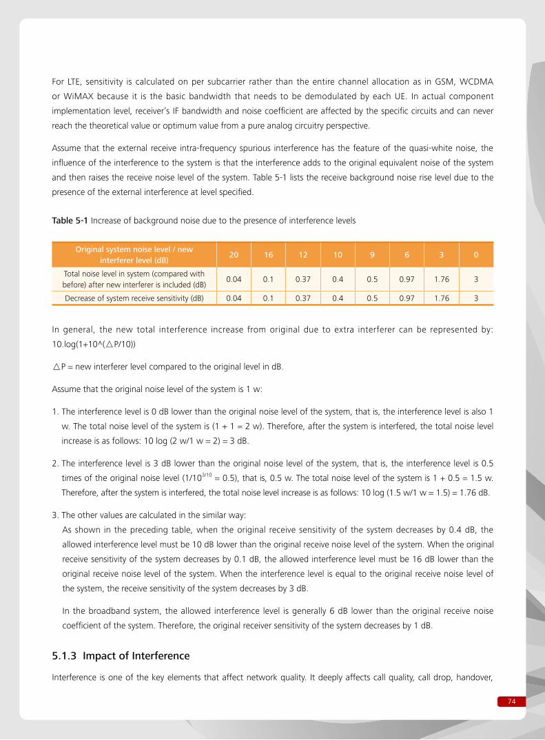
74
For LTE, sensitivity is calculated on per subcarrier rather than the entire channel allocation as in GSM, WCDMA
or WiMAX because it is the basic bandwidth that needs to be demodulated by each UE. In actual component
implementation level, receiver’s IF bandwidth and noise coefficient are affected by the specific circuits and can never
reach the theoretical value or optimum value from a pure analog circuitry perspective.
Assume that the external receive intra-frequency spurious interference has the feature of the quasi-white noise, the
influence of the interference to the system is that the interference adds to the original equivalent noise of the system
and then raises the receive noise level of the system. Table 5-1 lists the receive background noise rise level due to the
presence of the external interference at level specified.
Table 5-1 Increase of background noise due to the presence of interference levels
Original system noise level / new interferer level (dB)
20 16 12 10 9 6 3 0
Total noise level in system (compared with before) after new interferer is included (dB)
0.04 0.1 0.37 0.4 0.5 0.97 1.76 3
Decrease of system receive sensitivity (dB) 0.04 0.1 0.37 0.4 0.5 0.97 1.76 3
In general, the new total interference increase from original due to extra interferer can be represented by:
10.log(1+10^(△P/10))
△P = new interferer level compared to the original level in dB.
Assume that the original noise level of the system is 1 w:
1. The interference level is 0 dB lower than the original noise level of the system, that is, the interference level is also 1
w. The total noise level of the system is (1 + 1 = 2 w). Therefore, after the system is interfered, the total noise level
increase is as follows: 10 log (2 w/1 w = 2) = 3 dB.
2. The interference level is 3 dB lower than the original noise level of the system, that is, the interference level is 0.5
times of the original noise level (1/103/10 = 0.5), that is, 0.5 w. The total noise level of the system is 1 + 0.5 = 1.5 w.
Therefore, after the system is interfered, the total noise level increase is as follows: 10 log (1.5 w/1 w = 1.5) = 1.76 dB.
3. The other values are calculated in the similar way:
As shown in the preceding table, when the original receive sensitivity of the system decreases by 0.4 dB, the
allowed interference level must be 10 dB lower than the original receive noise level of the system. When the original
receive sensitivity of the system decreases by 0.1 dB, the allowed interference level must be 16 dB lower than the
original receive noise level of the system. When the interference level is equal to the original receive noise level of
the system, the receive sensitivity of the system decreases by 3 dB.
In the broadband system, the allowed interference level is generally 6 dB lower than the original receive noise
coefficient of the system. Therefore, the original receiver sensitivity of the system decreases by 1 dB.
5.1.3 Impact of Interference
Interference is one of the key elements that affect network quality. It deeply affects call quality, call drop, handover,
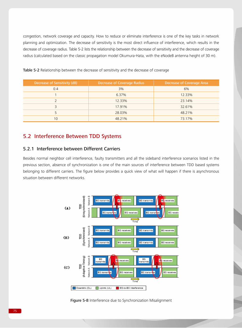
75
congestion, network coverage and capacity. How to reduce or eliminate interference is one of the key tasks in network
planning and optimization. The decrease of sensitivity is the most direct influence of interference, which results in the
decrease of coverage radius. Table 5-2 lists the relationship between the decrease of sensitivity and the decrease of coverage
radius (calculated based on the classic propagation model Okumura-Hata, with the eNodeB antenna height of 30 m).
Table 5-2 Relationship between the decrease of sensitivity and the decrease of coverage
Decrease of Sensitivity (dB) Decrease of Coverage Radius Decrease of Coverage Area
0.4 3% 6%
1 6.37% 12.33%
2 12.33% 23.14%
3 17.91% 32.61%
5 28.03% 48.21%
10 48.21% 73.17%
5.2 Interference Between TDD Systems
5.2.1 Interference between Different Carriers
Besides normal neighbor cell interference, faulty transmitters and all the sideband interference scenarios listed in the
previous section, absence of synchronization is one of the main sources of interference between TDD based systems
belonging to different carriers. The figure below provides a quick view of what will happen if there is asynchronous
situation between different networks.
Figure 5-8 Interference due to Synchronization Misalignment
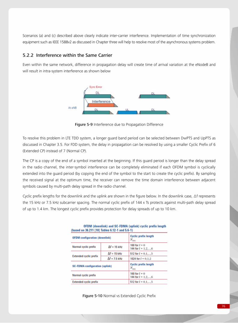
76
Scenarios (a) and (c) described above clearly indicate inter-carrier interference. Implementation of time synchronization
equipment such as IEEE 1588v2 as discussed in Chapter three will help to resolve most of the asynchronous systems problem.
5.2.2 Interference within the Same Carrier
Even within the same network, difference in propagation delay will create time of arrival variation at the eNodeB and
will result in intra-system interference as shown below
Figure 5-9 Interference due to Propagation Difference
To resolve this problem in LTE TDD system, a longer guard band period can be selected between DwPTS and UpPTS as
discussed in Chapter 3.5. For FDD system, the delay in propagation can be resolved by using a smaller Cyclic Prefix of 6
(Extended CP) instead of 7 (Normal CP).
The CP is a copy of the end of a symbol inserted at the beginning. If this guard period is longer than the delay spread
in the radio channel, the inter-symbol interference can be completely eliminated if each OFDM symbol is cyclically
extended into the guard period (by copying the end of the symbol to the start to create the cyclic prefix). By sampling
the received signal at the optimum time, the receiver can remove the time domain interference between adjacent
symbols caused by multi-path delay spread in the radio channel.
Cyclic prefix lengths for the downlink and the uplink are shown in the figure below. In the downlink case, Δf represents
the 15 kHz or 7.5 kHz subcarrier spacing. The normal cyclic prefix of 144 x Ts protects against multi-path delay spread
of up to 1.4 km. The longest cyclic prefix provides protection for delay spreads of up to 10 km.
Figure 5-10 Normal vs Extended Cyclic Prefix
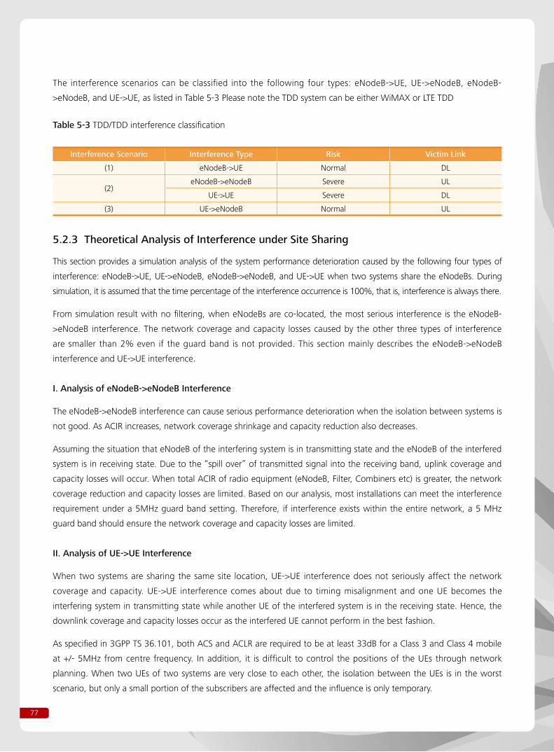
77
The interference scenarios can be classified into the following four types: eNodeB->UE, UE->eNodeB, eNodeB-
>eNodeB, and UE->UE, as listed in Table 5-3 Please note the TDD system can be either WiMAX or LTE TDD
5.2.3 Theoretical Analysis of Interference under Site Sharing
This section provides a simulation analysis of the system performance deterioration caused by the following four types of
interference: eNodeB->UE, UE->eNodeB, eNodeB->eNodeB, and UE->UE when two systems share the eNodeBs. During
simulation, it is assumed that the time percentage of the interference occurrence is 100%, that is, interference is always there.
From simulation result with no filtering, when eNodeBs are co-located, the most serious interference is the eNodeB-
>eNodeB interference. The network coverage and capacity losses caused by the other three types of interference
are smaller than 2% even if the guard band is not provided. This section mainly describes the eNodeB->eNodeB
interference and UE->UE interference.
I. Analysis of eNodeB->eNodeB Interference
The eNodeB->eNodeB interference can cause serious performance deterioration when the isolation between systems is
not good. As ACIR increases, network coverage shrinkage and capacity reduction also decreases.
Assuming the situation that eNodeB of the interfering system is in transmitting state and the eNodeB of the interfered
system is in receiving state. Due to the “spill over” of transmitted signal into the receiving band, uplink coverage and
capacity losses will occur. When total ACIR of radio equipment (eNodeB, Filter, Combiners etc) is greater, the network
coverage reduction and capacity losses are limited. Based on our analysis, most installations can meet the interference
requirement under a 5MHz guard band setting. Therefore, if interference exists within the entire network, a 5 MHz
guard band should ensure the network coverage and capacity losses are limited.
II. Analysis of UE->UE Interference
When two systems are sharing the same site location, UE->UE interference does not seriously affect the network
coverage and capacity. UE->UE interference comes about due to timing misalignment and one UE becomes the
interfering system in transmitting state while another UE of the interfered system is in the receiving state. Hence, the
downlink coverage and capacity losses occur as the interfered UE cannot perform in the best fashion.
As specified in 3GPP TS 36.101, both ACS and ACLR are required to be at least 33dB for a Class 3 and Class 4 mobile
at +/- 5MHz from centre frequency. In addition, it is difficult to control the positions of the UEs through network
planning. When two UEs of two systems are very close to each other, the isolation between the UEs is in the worst
scenario, but only a small portion of the subscribers are affected and the influence is only temporary.
Table 5-3 TDD/TDD interference classification
Interference Scenario Interference Type Risk Victim Link
(1) eNodeB->UE Normal DL
(2)eNodeB->eNodeB Severe UL
UE->UE Severe DL
(3) UE->eNodeB Normal UL
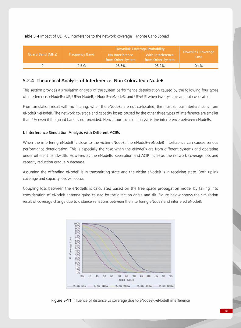
78
Table 5-4 Impact of UE->UE interference to the network coverage – Monte Carlo Spread
Guard Band (MHz) Frequency Band
Downlink Coverage ProbabilityDownlink Coverage
LossNo Interference from Other System
With Interference from Other System
0 2.5 G 98.6% 98.2% 0.4%
5.2.4 Theoretical Analysis of Interference: Non Colocated eNodeB
This section provides a simulation analysis of the system performance deterioration caused by the following four types
of interference: eNodeB->UE, UE->eNodeB, eNodeB->eNodeB, and UE->UE when two systems are not co-located.
From simulation result with no filtering, when the eNodeBs are not co-located, the most serious interference is from
eNodeB->eNodeB. The network coverage and capacity losses caused by the other three types of interference are smaller
than 2% even if the guard band is not provided. Hence, our focus of analysis is the interference between eNodeBs.
I. Interference Simulation Analysis with Different ACIRs
When the interfering eNodeB is close to the victim eNodeB, the eNodeB->eNodeB interference can causes serious
performance deterioration. This is especially the case when the eNodeBs are from different systems and operating
under different bandwidth. However, as the eNodeBs’ separation and ACIR increase, the network coverage loss and
capacity reduction gradually decrease.
Assuming the offending eNodeB is in transmitting state and the victim eNodeB is in receiving state. Both uplink
coverage and capacity loss will occur.
Coupling loss between the eNodeBs is calculated based on the free space propagation model by taking into
consideration of eNodeB antenna gains caused by the direction angle and tilt. Figure below shows the simulation
result of coverage change due to distance variations between the interfering eNodeB and interfered eNodeB.
Figure 5-11 Influence of distance vs coverage due to eNodeB->eNodeB interference
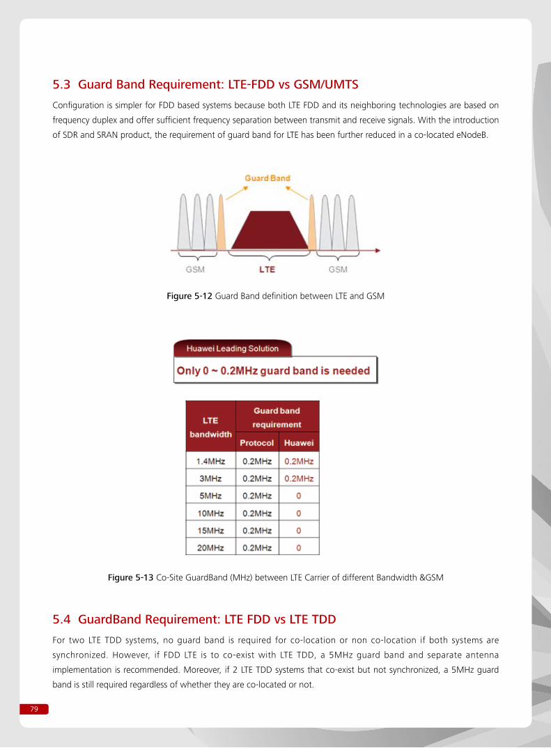
79
5.3 Guard Band Requirement: LTE-FDD vs GSM/UMTS
Configuration is simpler for FDD based systems because both LTE FDD and its neighboring technologies are based on
frequency duplex and offer sufficient frequency separation between transmit and receive signals. With the introduction
of SDR and SRAN product, the requirement of guard band for LTE has been further reduced in a co-located eNodeB.
Figure 5-12 Guard Band definition between LTE and GSM
Figure 5-13 Co-Site GuardBand (MHz) between LTE Carrier of different Bandwidth &GSM
5.4 GuardBand Requirement: LTE FDD vs LTE TDD
For two LTE TDD systems, no guard band is required for co-location or non co-location if both systems are
synchronized. However, if FDD LTE is to co-exist with LTE TDD, a 5MHz guard band and separate antenna
implementation is recommended. Moreover, if 2 LTE TDD systems that co-exist but not synchronized, a 5MHz guard
band is still required regardless of whether they are co-located or not.
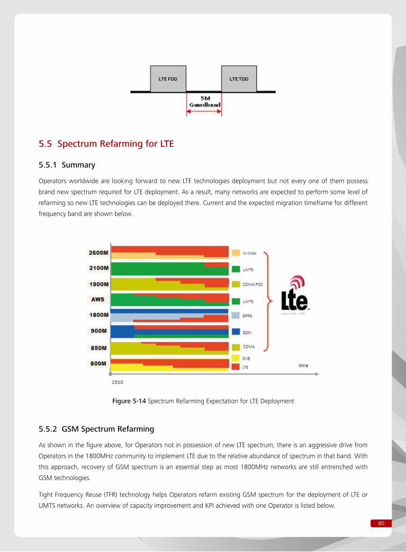
80
5.5 Spectrum Refarming for LTE
5.5.1 Summary
Operators worldwide are looking forward to new LTE technologies deployment but not every one of them possess
brand new spectrum required for LTE deployment. As a result, many networks are expected to perform some level of
refarming so new LTE technologies can be deployed there. Current and the expected migration timeframe for different
frequency band are shown below.
Figure 5-14 Spectrum Refarming Expectation for LTE Deployment
5.5.2 GSM Spectrum Refarming
As shown in the figure above, for Operators not in possession of new LTE spectrum, there is an aggressive drive from
Operators in the 1800MHz community to implement LTE due to the relative abundance of spectrum in that band. With
this approach, recovery of GSM spectrum is an essential step as most 1800MHz networks are still entrenched with
GSM technologies.
Tight Frequency Reuse (TFR) technology helps Operators refarm existing GSM spectrum for the deployment of LTE or
UMTS networks. An overview of capacity improvement and KPI achieved with one Operator is listed below.
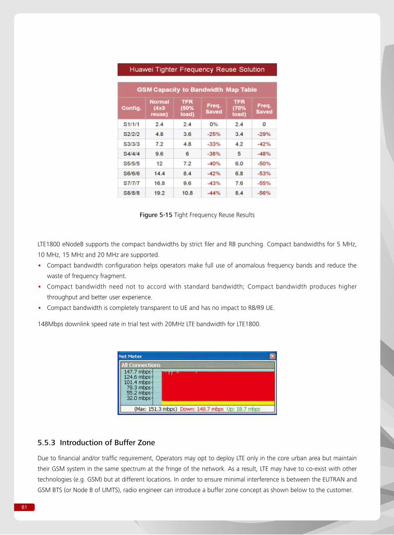
81
Figure 5-15 Tight Frequency Reuse Results
LTE1800 eNodeB supports the compact bandwidths by strict filer and RB punching. Compact bandwidths for 5 MHz,
10 MHz, 15 MHz and 20 MHz are supported.
Compact bandwidth configuration helps operators make full use of anomalous frequency bands and reduce the •
waste of frequency fragment.
Compact bandwidth need not to accord with standard bandwidth; Compact bandwidth produces higher •
throughput and better user experience.
Compact bandwidth is completely transparent to UE and has no impact to R8/R9 UE. •
148Mbps downlink speed rate in trial test with 20MHz LTE bandwidth for LTE1800.
5.5.3 Introduction of Buffer Zone
Due to financial and/or traffic requirement, Operators may opt to deploy LTE only in the core urban area but maintain
their GSM system in the same spectrum at the fringe of the network. As a result, LTE may have to co-exist with other
technologies (e.g. GSM) but at different locations. In order to ensure minimal interference is between the EUTRAN and
GSM BTS (or Node B of UMTS), radio engineer can introduce a buffer zone concept as shown below to the customer.
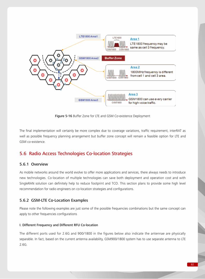
82
Figure 5-16 Buffer Zone for LTE and GSM Co-existence Deployment
The final implementation will certainly be more complex due to coverage variations, traffic requirement, interRAT as
well as possible frequency planning arrangement but buffer zone concept will remain a feasible option for LTE and
GSM co-existence.
5.6 Radio Access Technologies Co-location Strategies
5.6.1 Overview
As mobile networks around the world evolve to offer more applications and services, there always needs to introduce
new technologies. Co-location of multiple technologies can save both deployment and operation cost and with
SingleRAN solution can definitely help to reduce footprint and TCO. This section plans to provide some high level
recommendation for radio engineers on co-location strategies and configurations.
5.6.2 GSM-LTE Co-Location Examples
Please note the following examples are just some of the possible frequencies combinations but the same concept can
apply to other frequencies configurations
I. Different Frequency and Different RFU Co-location
The different ports used for 2.6G and 900/1800 in the figures below also indicate the antennae are physically
separable. In fact, based on the current antenna availability, GSM900/1800 system has to use separate antenna to LTE
2.6G.
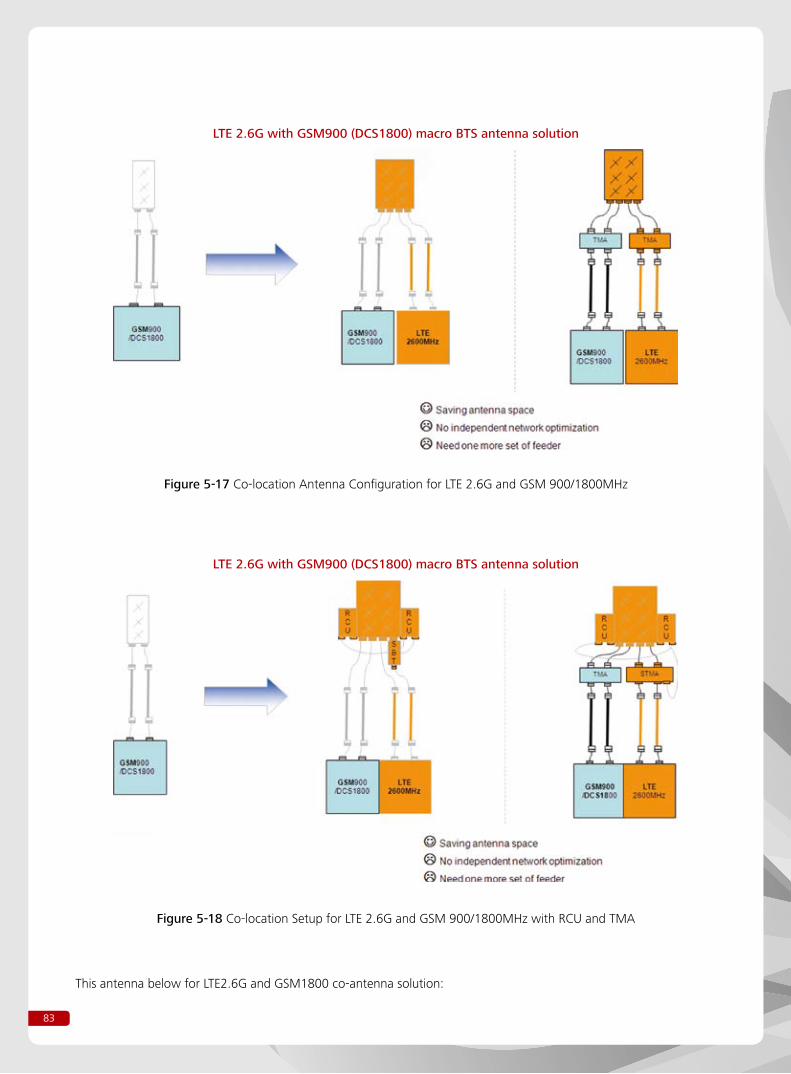
83
Figure 5-17 Co-location Antenna Configuration for LTE 2.6G and GSM 900/1800MHz
LTE 2.6G with GSM900 (DCS1800) macro BTS antenna solution
Figure 5-18 Co-location Setup for LTE 2.6G and GSM 900/1800MHz with RCU and TMA
LTE 2.6G with GSM900 (DCS1800) macro BTS antenna solution
This antenna below for LTE2.6G and GSM1800 co-antenna solution:
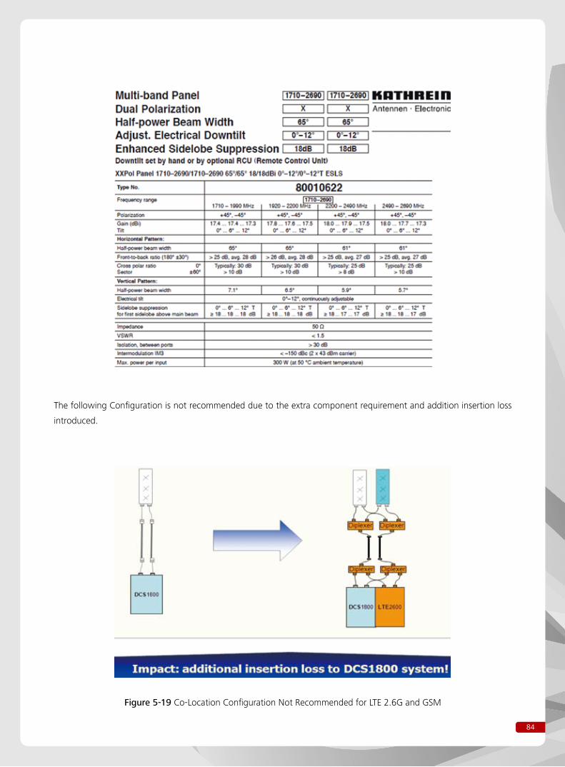
84
Figure 5-19 Co-Location Configuration Not Recommended for LTE 2.6G and GSM
The following Configuration is not recommended due to the extra component requirement and addition insertion loss
introduced.
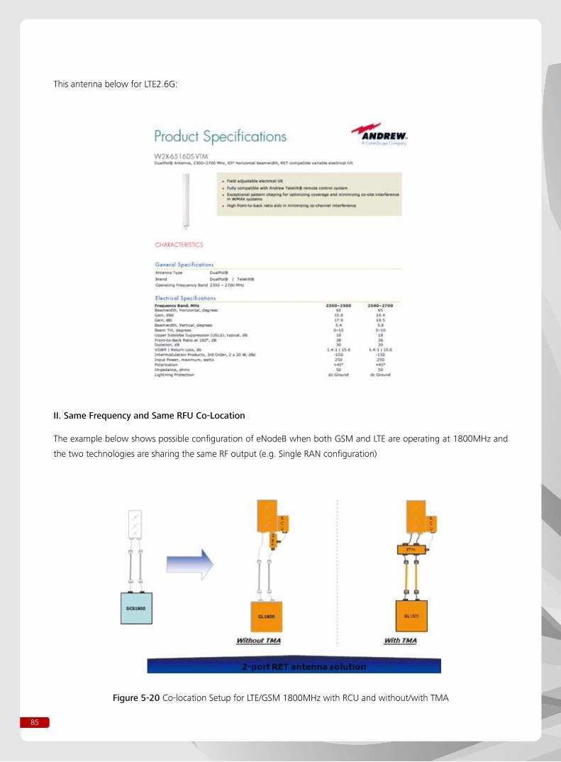
85
This antenna below for LTE2.6G:
II. Same Frequency and Same RFU Co-Location
The example below shows possible configuration of eNodeB when both GSM and LTE are operating at 1800MHz and
the two technologies are sharing the same RF output (e.g. Single RAN configuration)
Figure 5-20 Co-location Setup for LTE/GSM 1800MHz with RCU and without/with TMA
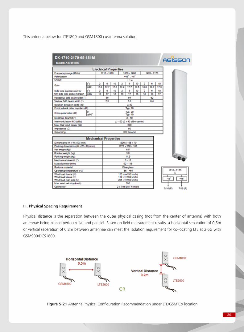
86
This antenna below for LTE1800 and GSM1800 co-antenna solution:
III. Physical Spacing Requirement
Physical distance is the separation between the outer physical casing (not from the center of antenna) with both
antennae being placed perfectly flat and parallel. Based on field measurement results, a horizontal separation of 0.5m
or vertical separation of 0.2m between antennae can meet the isolation requirement for co-locating LTE at 2.6G with
GSM900/DCS1800.
Figure 5-21 Antenna Physical Configuration Recommendation under LTE/GSM Co-location
OR
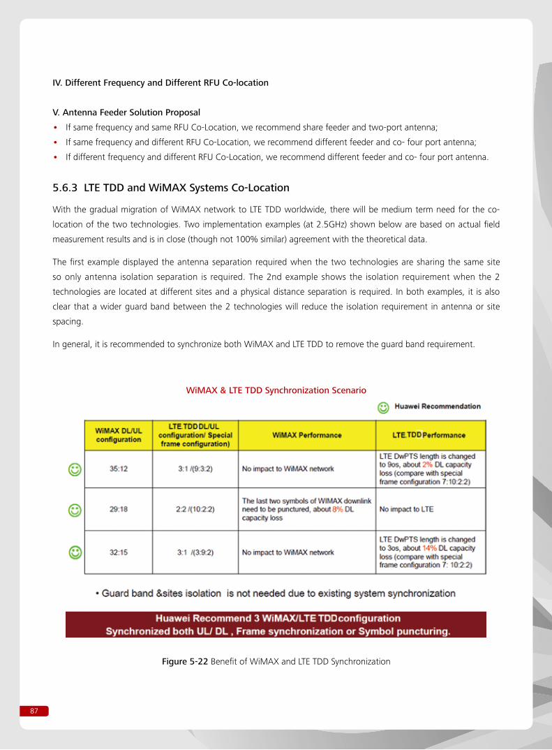
87
IV. Different Frequency and Different RFU Co-location
V. Antenna Feeder Solution Proposal
If same frequency and same RFU Co-Location, we recommend share feeder and two-port antenna; •
If same frequency and different RFU Co-Location, we recommend different feeder and co- four port antenna; •
If different frequency and different RFU Co-Location, we recommend different feeder and co- four port antenna. •
5.6.3 LTE TDD and WiMAX Systems Co-Location
With the gradual migration of WiMAX network to LTE TDD worldwide, there will be medium term need for the co-
location of the two technologies. Two implementation examples (at 2.5GHz) shown below are based on actual field
measurement results and is in close (though not 100% similar) agreement with the theoretical data.
The first example displayed the antenna separation required when the two technologies are sharing the same site
so only antenna isolation separation is required. The 2nd example shows the isolation requirement when the 2
technologies are located at different sites and a physical distance separation is required. In both examples, it is also
clear that a wider guard band between the 2 technologies will reduce the isolation requirement in antenna or site
spacing.
In general, it is recommended to synchronize both WiMAX and LTE TDD to remove the guard band requirement.
Figure 5-22 Benefit of WiMAX and LTE TDD Synchronization
WiMAX & LTE TDD Synchronization Scenario
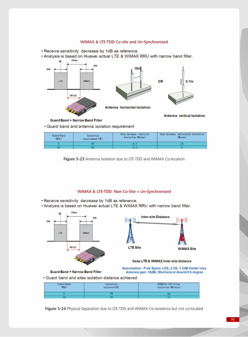
88
Figure 5-23 Antenna Isolation due to LTE TDD and WiMAX Co-location
WiMAX & LTE-TDD Co-site and Un-Synchronized
Figure 5-24 Physical Separation due to LTE TDD and WiMAX Co-existence but not co-located
WiMAX & LTE-TDD: Non Co-Site + Un-Synchronized
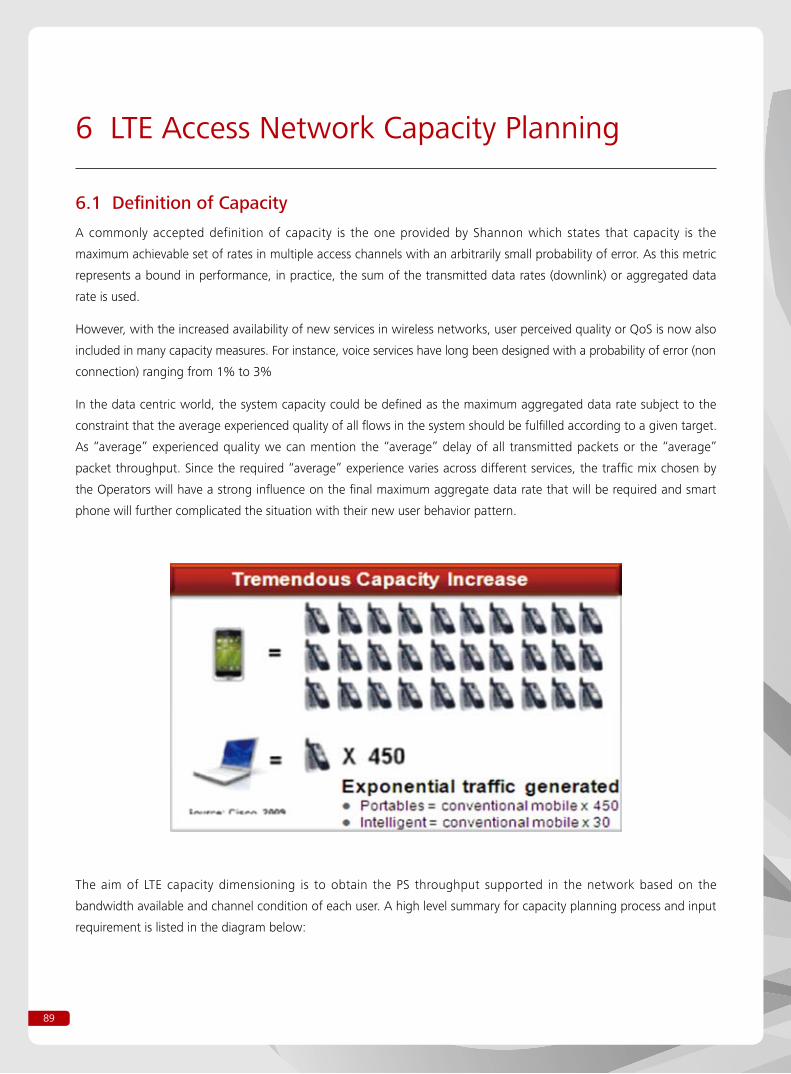
89
6 LTE Access Network Capacity Planning
6.1 Definition of Capacity
A commonly accepted definition of capacity is the one provided by Shannon which states that capacity is the
maximum achievable set of rates in multiple access channels with an arbitrarily small probability of error. As this metric
represents a bound in performance, in practice, the sum of the transmitted data rates (downlink) or aggregated data
rate is used.
However, with the increased availability of new services in wireless networks, user perceived quality or QoS is now also
included in many capacity measures. For instance, voice services have long been designed with a probability of error (non
connection) ranging from 1% to 3%
In the data centric world, the system capacity could be defined as the maximum aggregated data rate subject to the
constraint that the average experienced quality of all flows in the system should be fulfilled according to a given target.
As “average” experienced quality we can mention the “average” delay of all transmitted packets or the “average”
packet throughput. Since the required “average” experience varies across different services, the traffic mix chosen by
the Operators will have a strong influence on the final maximum aggregate data rate that will be required and smart
phone will further complicated the situation with their new user behavior pattern.
The aim of LTE capacity dimensioning is to obtain the PS throughput supported in the network based on the
bandwidth available and channel condition of each user. A high level summary for capacity planning process and input
requirement is listed in the diagram below:
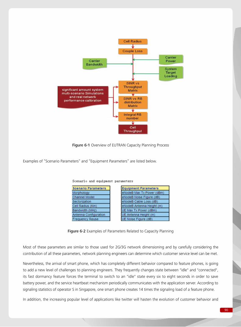
90
Figure 6-1 Overview of EUTRAN Capacity Planning Process
Figure 6-2 Examples of Parameters Related to Capacity Planning
Examples of “Scenario Parameters” and “Equipment Parameters” are listed below.
Most of these parameters are similar to those used for 2G/3G network dimensioning and by carefully considering the
contribution of all these parameters, network planning engineers can determine which customer service level can be met.
Nevertheless, the arrival of smart phone, which has completely different behavior compared to feature phones, is going
to add a new level of challenges to planning engineers. They frequently changes state between "idle" and "connected",
its fast dormancy feature forces the terminal to switch to an "idle" state every six to eight seconds in order to save
battery power, and the service heartbeat mechanism periodically communicates with the application server. According to
signaling statistics of operator S in Singapore, one smart phone creates 14 times the signaling load of a feature phone.
In addition, the increasing popular level of applications like twitter will hasten the evolution of customer behavior and
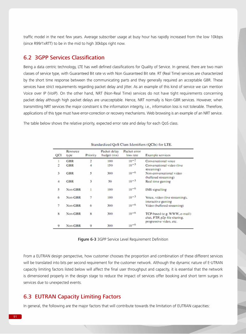
91
traffic model in the next few years. Average subscriber usage at busy hour has rapidly increased from the low 10kbps
(since R99/1xRTT) to be in the mid to high 30kbps right now.
6.2 3GPP Services Classification
Being a data centric technology, LTE has well defined classifications for Quality of Service. In general, there are two main
classes of service type, with Guaranteed Bit rate vs with Non Guaranteed Bit rate. RT (Real Time) services are characterized
by the short time response between the communicating parts and they generally required an acceptable GBR. These
services have strict requirements regarding packet delay and jitter. As an example of this kind of service we can mention
Voice over IP (VoIP). On the other hand, NRT (Non-Real Time) services do not have tight requirements concerning
packet delay although high packet delays are unacceptable. Hence, NRT normally is Non-GBR services. However, when
transmitting NRT services the major constraint is the information integrity, i.e., information loss is not tolerable. Therefore,
applications of this type must have error-correction or recovery mechanisms. Web browsing is an example of an NRT service.
The table below shows the relative priority, expected error rate and delay for each QoS class.
From a EUTRAN design perspective, how customer chooses the proportion and combination of these different services
will be translated into bits per second requirement for the customer network. Although the dynamic nature of E-UTRAN
capacity limiting factors listed below will affect the final user throughput and capacity, it is essential that the network
is dimensioned properly in the design stage to reduce the impact of services offer booking and short term surges in
services due to unexpected events.
6.3 EUTRAN Capacity Limiting Factors
In general, the following are the major factors that will contribute towards the limitation of EUTRAN capacities:
Figure 6-3 3GPP Service Level Requirement Definition
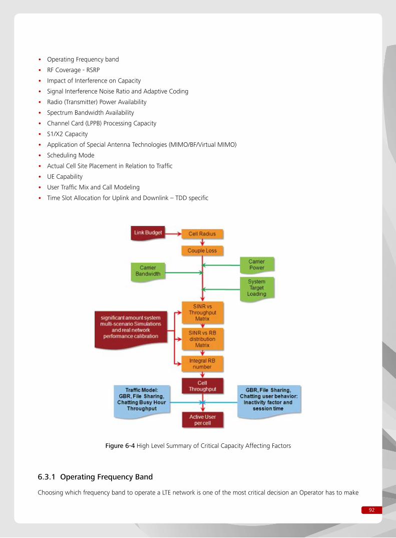
92
Figure 6-4 High Level Summary of Critical Capacity Affecting Factors
Operating Frequency band •
RF Coverage - RSRP •
Impact of Interference on Capacity •
Signal Interference Noise Ratio and Adaptive Coding •
Radio (Transmitter) Power Availability •
Spectrum Bandwidth Availability •
Channel Card (LPPB) Processing Capacity •
S1/X2 Capacity •
Application of Special Antenna Technologies (MIMO/BF/Virtual MIMO) •
Scheduling Mode •
Actual Cell Site Placement in Relation to Traffic •
UE Capability •
User Traffic Mix and Call Modeling •
Time Slot Allocation for Uplink and Downlink – TDD specific •
6.3.1 Operating Frequency Band
Choosing which frequency band to operate a LTE network is one of the most critical decision an Operator has to make
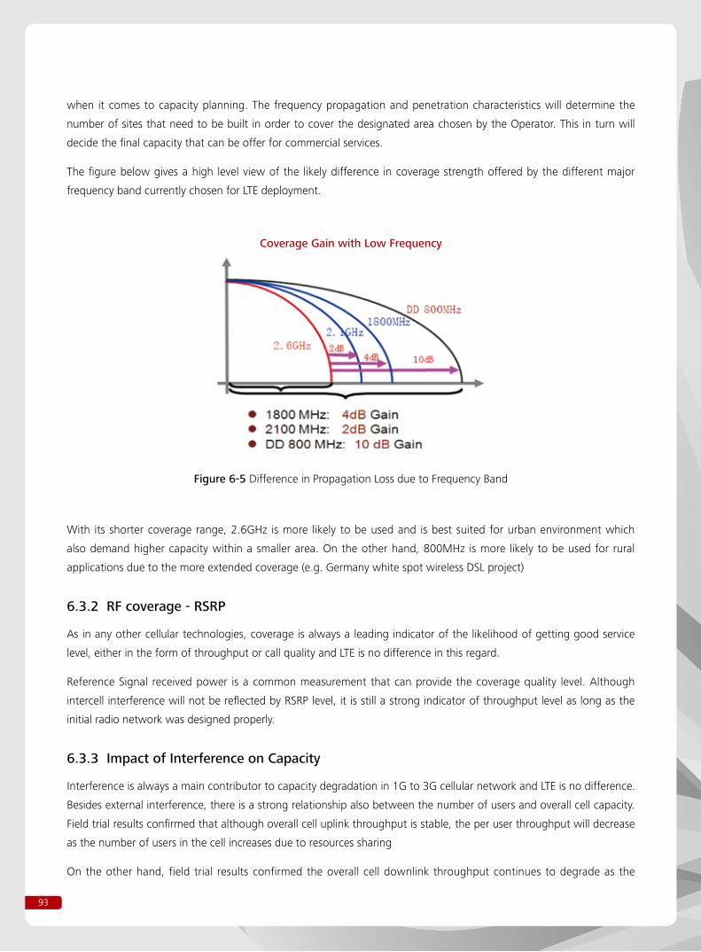
93
when it comes to capacity planning. The frequency propagation and penetration characteristics will determine the
number of sites that need to be built in order to cover the designated area chosen by the Operator. This in turn will
decide the final capacity that can be offer for commercial services.
The figure below gives a high level view of the likely difference in coverage strength offered by the different major
frequency band currently chosen for LTE deployment.
Figure 6-5 Difference in Propagation Loss due to Frequency Band
Coverage Gain with Low Frequency
With its shorter coverage range, 2.6GHz is more likely to be used and is best suited for urban environment which
also demand higher capacity within a smaller area. On the other hand, 800MHz is more likely to be used for rural
applications due to the more extended coverage (e.g. Germany white spot wireless DSL project)
6.3.2 RF coverage - RSRP
As in any other cellular technologies, coverage is always a leading indicator of the likelihood of getting good service
level, either in the form of throughput or call quality and LTE is no difference in this regard.
Reference Signal received power is a common measurement that can provide the coverage quality level. Although
intercell interference will not be reflected by RSRP level, it is still a strong indicator of throughput level as long as the
initial radio network was designed properly.
6.3.3 Impact of Interference on Capacity
Interference is always a main contributor to capacity degradation in 1G to 3G cellular network and LTE is no difference.
Besides external interference, there is a strong relationship also between the number of users and overall cell capacity.
Field trial results confirmed that although overall cell uplink throughput is stable, the per user throughput will decrease
as the number of users in the cell increases due to resources sharing
On the other hand, field trial results confirmed the overall cell downlink throughput continues to degrade as the
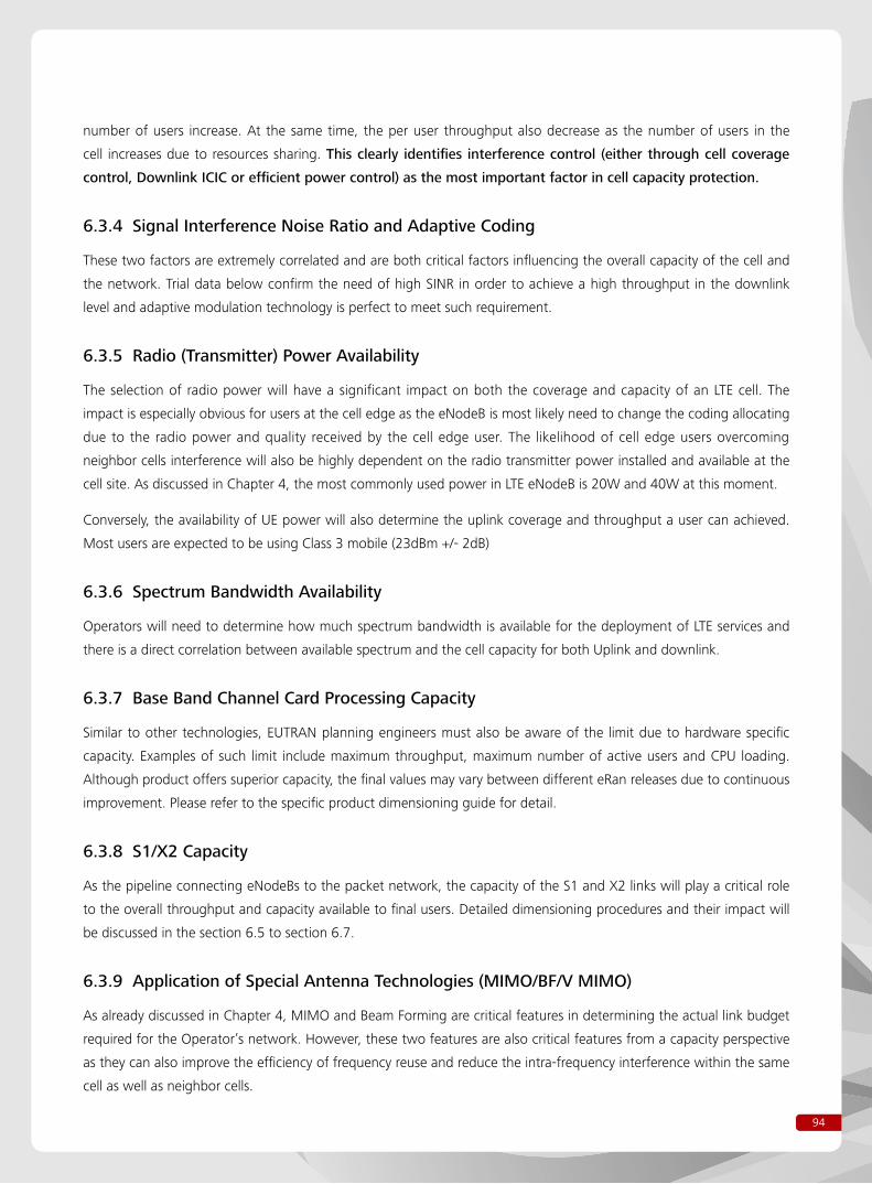
94
number of users increase. At the same time, the per user throughput also decrease as the number of users in the
cell increases due to resources sharing. This clearly identifies interference control (either through cell coverage
control, Downlink ICIC or efficient power control) as the most important factor in cell capacity protection.
6.3.4 Signal Interference Noise Ratio and Adaptive Coding
These two factors are extremely correlated and are both critical factors influencing the overall capacity of the cell and
the network. Trial data below confirm the need of high SINR in order to achieve a high throughput in the downlink
level and adaptive modulation technology is perfect to meet such requirement.
6.3.5 Radio (Transmitter) Power Availability
The selection of radio power will have a significant impact on both the coverage and capacity of an LTE cell. The
impact is especially obvious for users at the cell edge as the eNodeB is most likely need to change the coding allocating
due to the radio power and quality received by the cell edge user. The likelihood of cell edge users overcoming
neighbor cells interference will also be highly dependent on the radio transmitter power installed and available at the
cell site. As discussed in Chapter 4, the most commonly used power in LTE eNodeB is 20W and 40W at this moment.
Conversely, the availability of UE power will also determine the uplink coverage and throughput a user can achieved.
Most users are expected to be using Class 3 mobile (23dBm +/- 2dB)
6.3.6 Spectrum Bandwidth Availability
Operators will need to determine how much spectrum bandwidth is available for the deployment of LTE services and
there is a direct correlation between available spectrum and the cell capacity for both Uplink and downlink.
6.3.7 Base Band Channel Card Processing Capacity
Similar to other technologies, EUTRAN planning engineers must also be aware of the limit due to hardware specific
capacity. Examples of such limit include maximum throughput, maximum number of active users and CPU loading.
Although product offers superior capacity, the final values may vary between different eRan releases due to continuous
improvement. Please refer to the specific product dimensioning guide for detail.
6.3.8 S1/X2 Capacity
As the pipeline connecting eNodeBs to the packet network, the capacity of the S1 and X2 links will play a critical role
to the overall throughput and capacity available to final users. Detailed dimensioning procedures and their impact will
be discussed in the section 6.5 to section 6.7.
6.3.9 Application of Special Antenna Technologies (MIMO/BF/V MIMO)
As already discussed in Chapter 4, MIMO and Beam Forming are critical features in determining the actual link budget
required for the Operator’s network. However, these two features are also critical features from a capacity perspective
as they can also improve the efficiency of frequency reuse and reduce the intra-frequency interference within the same
cell as well as neighbor cells.
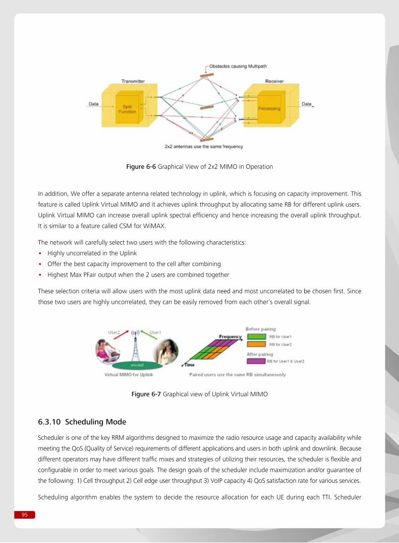
95
Figure 6-6 Graphical View of 2x2 MIMO in Operation
In addition, We offer a separate antenna related technology in uplink, which is focusing on capacity improvement. This
feature is called Uplink Virtual MIMO and it achieves uplink throughput by allocating same RB for different uplink users.
Uplink Virtual MIMO can increase overall uplink spectral efficiency and hence increasing the overall uplink throughput.
It is similar to a feature called CSM for WiMAX.
The network will carefully select two users with the following characteristics:
Highly uncorrelated in the Uplink •
Offer the best capacity improvement to the cell after combining •
Highest Max PFair output when the 2 users are combined together •
These selection criteria will allow users with the most uplink data need and most uncorrelated to be chosen first. Since
those two users are highly uncorrelated, they can be easily removed from each other’s overall signal.
Figure 6-7 Graphical view of Uplink Virtual MIMO
6.3.10 Scheduling Mode
Scheduler is one of the key RRM algorithms designed to maximize the radio resource usage and capacity availability while
meeting the QoS (Quality of Service) requirements of different applications and users in both uplink and downlink. Because
different operators may have different traffic mixes and strategies of utilizing their resources, the scheduler is flexible and
configurable in order to meet various goals. The design goals of the scheduler include maximization and/or guarantee of
the following: 1) Cell throughput 2) Cell edge user throughput 3) VoIP capacity 4) QoS satisfaction rate for various services.
Scheduling algorithm enables the system to decide the resource allocation for each UE during each TTI. Scheduler
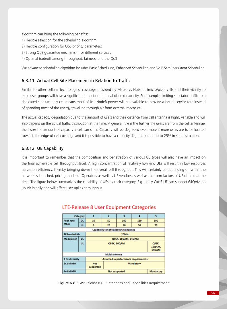
96
Figure 6-8 3GPP Release 8 UE Categories and Capabilities Requirement
algorithm can bring the following benefits:
1) Flexible selection for the scheduling algorithm
2) Flexible configuration for QoS priority parameters
3) Strong QoS guarantee mechanism for different services
4) Optimal tradeoff among throughput, fairness, and the QoS
We advanced scheduling algorithm includes Basic Scheduling, Enhanced Scheduling and VoIP Semi-persistent Scheduling.
6.3.11 Actual Cell Site Placement in Relation to Traffic
Similar to other cellular technologies, coverage provided by Macro vs Hotspot (micro/pico) cells and their vicinity to
main user groups will have a significant impact on the final offered capacity. For example, limiting spectator traffic to a
dedicated stadium only cell means most of its eNodeB power will be available to provide a better service rate instead
of spending most of the energy travelling through air from external macro cell.
The actual capacity degradation due to the amount of users and their distance from cell antenna is highly variable and will
also depend on the actual traffic distribution at the time. A general rule is the further the users are from the cell antennae,
the lesser the amount of capacity a cell can offer. Capacity will be degraded even more if more users are to be located
towards the edge of cell coverage and it is possible to have a capacity degradation of up to 25% in some situation.
6.3.12 UE Capability
It is important to remember that the composition and penetration of various UE types will also have an impact on
the final achievable cell throughput level. A high concentration of relatively low end UEs will result in low resources
utilization efficiency, thereby bringing down the overall cell throughput. This will certainly be depending on when the
network is launched, pricing model of Operators as well as UE vendors as well as the form factors of UE offered at the
time. The figure below summarizes the capability of UEs by their category. E.g. only Cat-5 UE can support 64QAM on
uplink initially and will affect user uplink throughput.
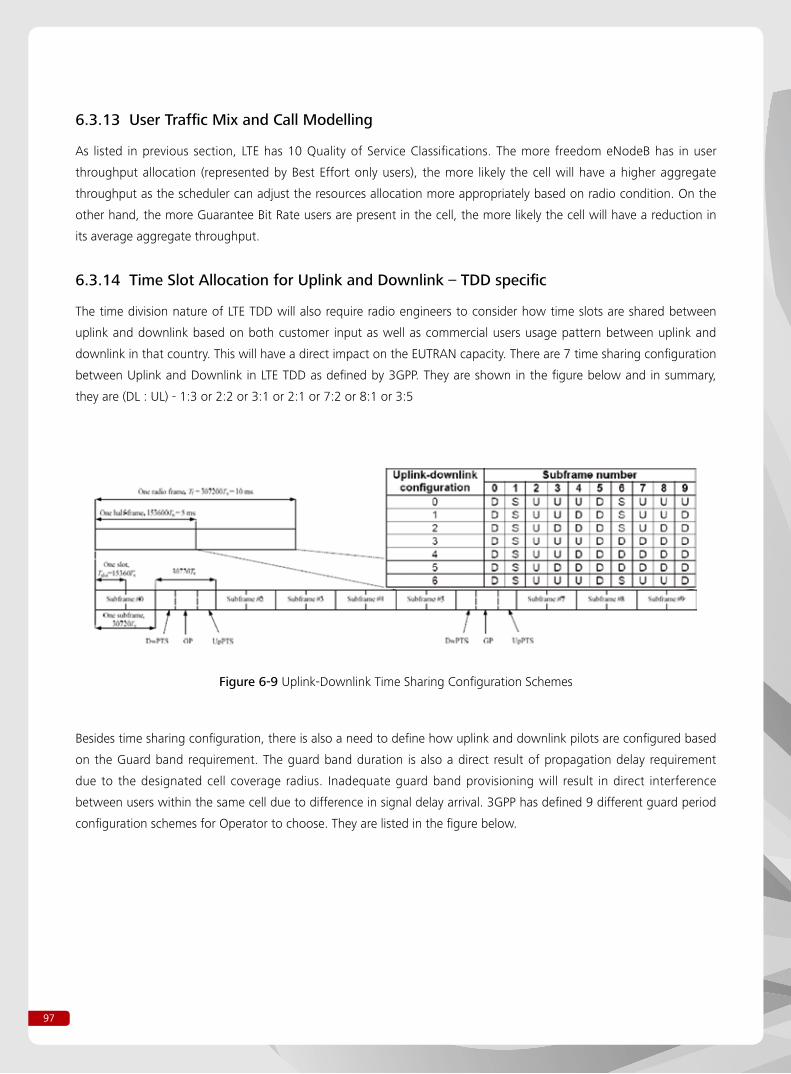
97
6.3.13 User Traffic Mix and Call Modelling
As listed in previous section, LTE has 10 Quality of Service Classifications. The more freedom eNodeB has in user
throughput allocation (represented by Best Effort only users), the more likely the cell will have a higher aggregate
throughput as the scheduler can adjust the resources allocation more appropriately based on radio condition. On the
other hand, the more Guarantee Bit Rate users are present in the cell, the more likely the cell will have a reduction in
its average aggregate throughput.
6.3.14 Time Slot Allocation for Uplink and Downlink – TDD specific
The time division nature of LTE TDD will also require radio engineers to consider how time slots are shared between
uplink and downlink based on both customer input as well as commercial users usage pattern between uplink and
downlink in that country. This will have a direct impact on the EUTRAN capacity. There are 7 time sharing configuration
between Uplink and Downlink in LTE TDD as defined by 3GPP. They are shown in the figure below and in summary,
they are (DL : UL) - 1:3 or 2:2 or 3:1 or 2:1 or 7:2 or 8:1 or 3:5
Besides time sharing configuration, there is also a need to define how uplink and downlink pilots are configured based
on the Guard band requirement. The guard band duration is also a direct result of propagation delay requirement
due to the designated cell coverage radius. Inadequate guard band provisioning will result in direct interference
between users within the same cell due to difference in signal delay arrival. 3GPP has defined 9 different guard period
configuration schemes for Operator to choose. They are listed in the figure below.
Figure 6-9 Uplink-Downlink Time Sharing Configuration Schemes
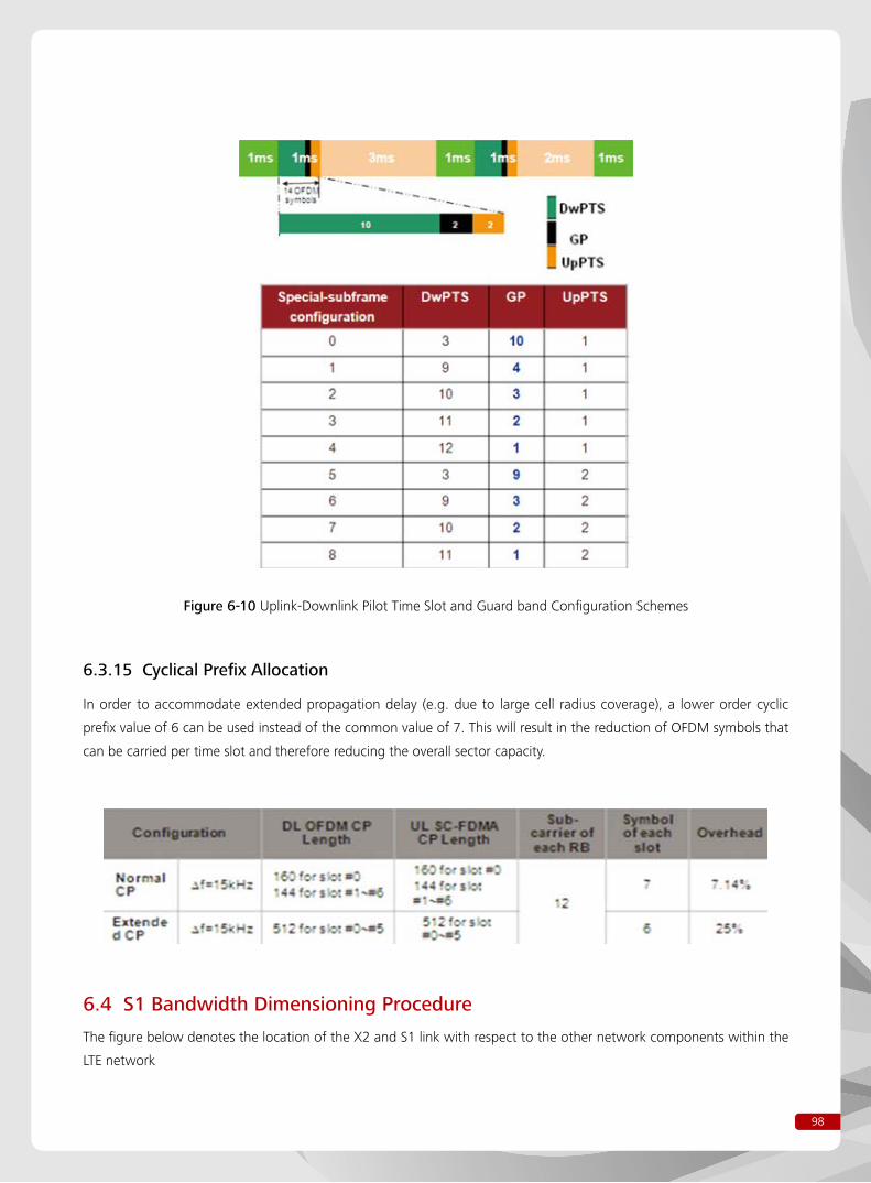
98
Figure 6-10 Uplink-Downlink Pilot Time Slot and Guard band Configuration Schemes
6.4 S1 Bandwidth Dimensioning Procedure
The figure below denotes the location of the X2 and S1 link with respect to the other network components within the
LTE network
6.3.15 Cyclical Prefix Allocation
In order to accommodate extended propagation delay (e.g. due to large cell radius coverage), a lower order cyclic
prefix value of 6 can be used instead of the common value of 7. This will result in the reduction of OFDM symbols that
can be carried per time slot and therefore reducing the overall sector capacity.
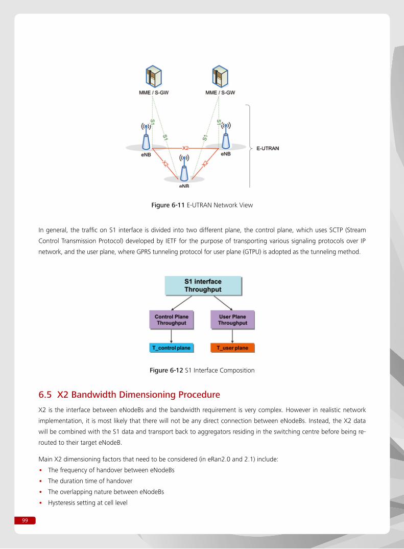
99
In general, the traffic on S1 interface is divided into two different plane, the control plane, which uses SCTP (Stream
Control Transmission Protocol) developed by IETF for the purpose of transporting various signaling protocols over IP
network, and the user plane, where GPRS tunneling protocol for user plane (GTPU) is adopted as the tunneling method.
Figure 6-11 E-UTRAN Network View
Figure 6-12 S1 Interface Composition
6.5 X2 Bandwidth Dimensioning Procedure
X2 is the interface between eNodeBs and the bandwidth requirement is very complex. However in realistic network
implementation, it is most likely that there will not be any direct connection between eNodeBs. Instead, the X2 data
will be combined with the S1 data and transport back to aggregators residing in the switching centre before being re-
routed to their target eNodeB.
Main X2 dimensioning factors that need to be considered (in eRan2.0 and 2.1) include:
The frequency of handover between eNodeBs •
The duration time of handover •
The overlapping nature between eNodeBs •
Hysteresis setting at cell level •
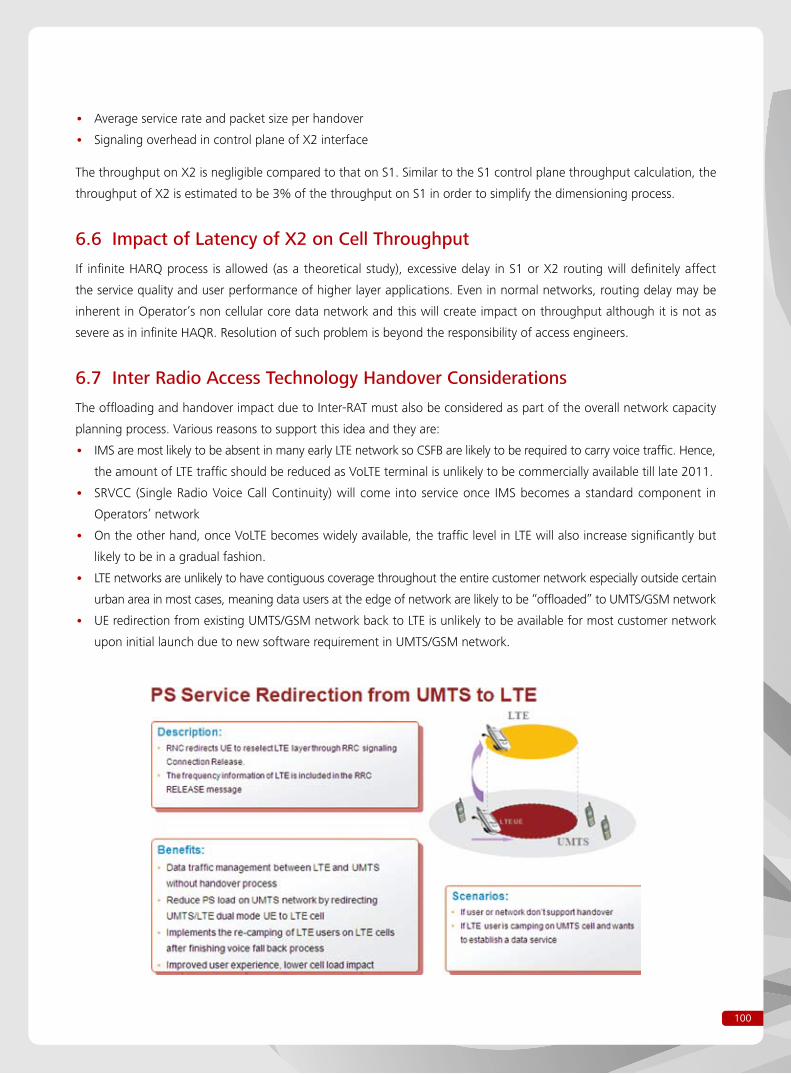
100
Average service rate and packet size per handover •
Signaling overhead in control plane of X2 interface •
The throughput on X2 is negligible compared to that on S1. Similar to the S1 control plane throughput calculation, the
throughput of X2 is estimated to be 3% of the throughput on S1 in order to simplify the dimensioning process.
6.6 Impact of Latency of X2 on Cell Throughput
If infinite HARQ process is allowed (as a theoretical study), excessive delay in S1 or X2 routing will definitely affect
the service quality and user performance of higher layer applications. Even in normal networks, routing delay may be
inherent in Operator’s non cellular core data network and this will create impact on throughput although it is not as
severe as in infinite HAQR. Resolution of such problem is beyond the responsibility of access engineers.
6.7 Inter Radio Access Technology Handover Considerations
The offloading and handover impact due to Inter-RAT must also be considered as part of the overall network capacity
planning process. Various reasons to support this idea and they are:
IMS are most likely to be absent in many early LTE network so CSFB are likely to be required to carry voice traffic. Hence, •
the amount of LTE traffic should be reduced as VoLTE terminal is unlikely to be commercially available till late 2011.
SRVCC (Single Radio Voice Call Continuity) will come into service once IMS becomes a standard component in •
Operators’ network
On the other hand, once VoLTE becomes widely available, the traffic level in LTE will also increase significantly but •
likely to be in a gradual fashion.
LTE networks are unlikely to have contiguous coverage throughout the entire customer network especially outside certain •
urban area in most cases, meaning data users at the edge of network are likely to be “offloaded” to UMTS/GSM network
UE redirection from existing UMTS/GSM network back to LTE is unlikely to be available for most customer network •
upon initial launch due to new software requirement in UMTS/GSM network.
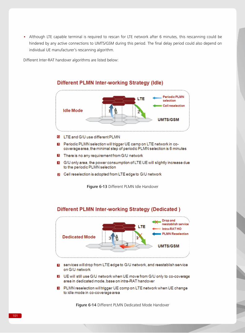
101
Although LTE capable terminal is required to rescan for LTE network after 6 minutes, this rescanning could be •
hindered by any active connections to UMTS/GSM during this period. The final delay period could also depend on
individual UE manufacturer’s rescanning algorithm.
Different Inter-RAT handover algorithms are listed below:
Figure 6-13 Different PLMN Idle Handover
Figure 6-14 Different PLMN Dedicated Mode Handover
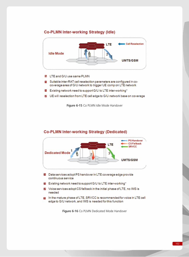
102
Figure 6-15 Co PLMN Idle Mode Handover
Figure 6-16 Co PLMN Dedicated Mode Handover
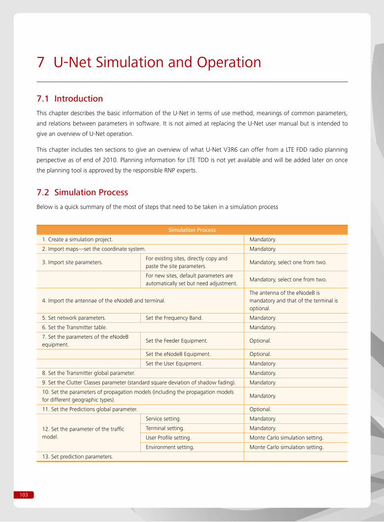
103
7 U-Net Simulation and Operation
7.1 Introduction
This chapter describes the basic information of the U-Net in terms of use method, meanings of common parameters,
and relations between parameters in software. It is not aimed at replacing the U-Net user manual but is intended to
give an overview of U-Net operation.
This chapter includes ten sections to give an overview of what U-Net V3R6 can offer from a LTE FDD radio planning
perspective as of end of 2010. Planning information for LTE TDD is not yet available and will be added later on once
the planning tool is approved by the responsible RNP experts.
7.2 Simulation Process
Below is a quick summary of the most of steps that need to be taken in a simulation process
Simulation Process
1. Create a simulation project. Mandatory.
2. Import maps—set the coordinate system. Mandatory.
3. Import site parameters.For existing sites, directly copy and paste the site parameters.
Mandatory, select one from two.
For new sites, default parameters are automatically set but need adjustment.
Mandatory, select one from two.
4. Import the antennae of the eNodeB and terminal.The antenna of the eNodeB is mandatory and that of the terminal is optional.
5. Set network parameters. Set the Frequency Band. Mandatory.
6. Set the Transmitter table. Mandatory.
7. Set the parameters of the eNodeB equipment.
Set the Feeder Equipment. Optional.
Set the eNodeB Equipment. Optional.
Set the User Equipment. Mandatory.
8. Set the Transmitter global parameter. Mandatory.
9. Set the Clutter Classes parameter (standard square deviation of shadow fading). Mandatory.
10. Set the parameters of propagation models (including the propagation models for different geographic types).
Mandatory.
11. Set the Predictions global parameter. Optional.
12. Set the parameter of the traffic model.
Service setting. Mandatory.
Terminal setting. Mandatory.
User Profile setting. Monte Carlo simulation setting.
Environment setting. Monte Carlo simulation setting.
13. Set prediction parameters.
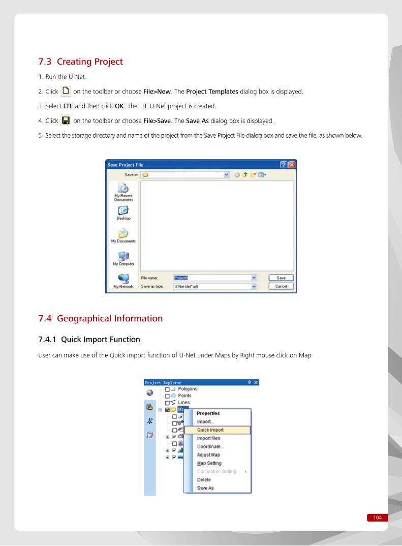
104
7.3 Creating Project
1. Run the U-Net.
2. Click on the toolbar or choose File>New. The Project Templates dialog box is displayed.
3. Select LTE and then click OK. The LTE U-Net project is created.
4. Click on the toolbar or choose File>Save. The Save As dialog box is displayed.
5. Select the storage directory and name of the project from the Save Project File dialog box and save the file, as shown below.
7.4 Geographical Information
7.4.1 Quick Import Function
User can make use of the Quick import function of U-Net under Maps by Right mouse click on Map
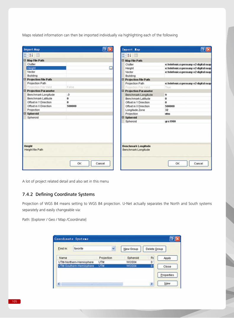
105
Maps related information can then be imported individually via highlighting each of the following
A lot of project related detail and also set in this menu
7.4.2 Defining Coordinate Systems
Projection of WGS 84 means setting to WGS 84 projection. U-Net actually separates the North and South systems
separately and easily changeable via:
Path: [Explorer / Geo / Map /Coordinate]
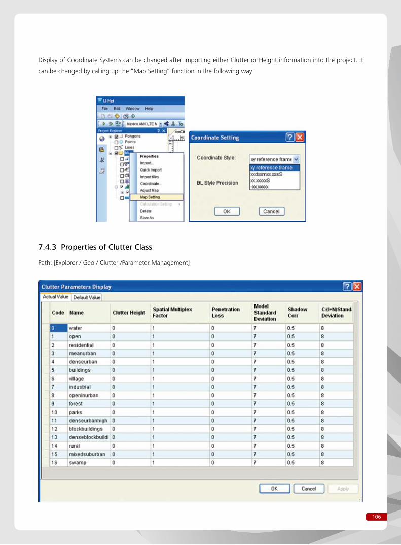
106
Display of Coordinate Systems can be changed after importing either Clutter or Height information into the project. It
can be changed by calling up the “Map Setting” function in the following way
7.4.3 Properties of Clutter Class
Path: [Explorer / Geo / Clutter /Parameter Management]
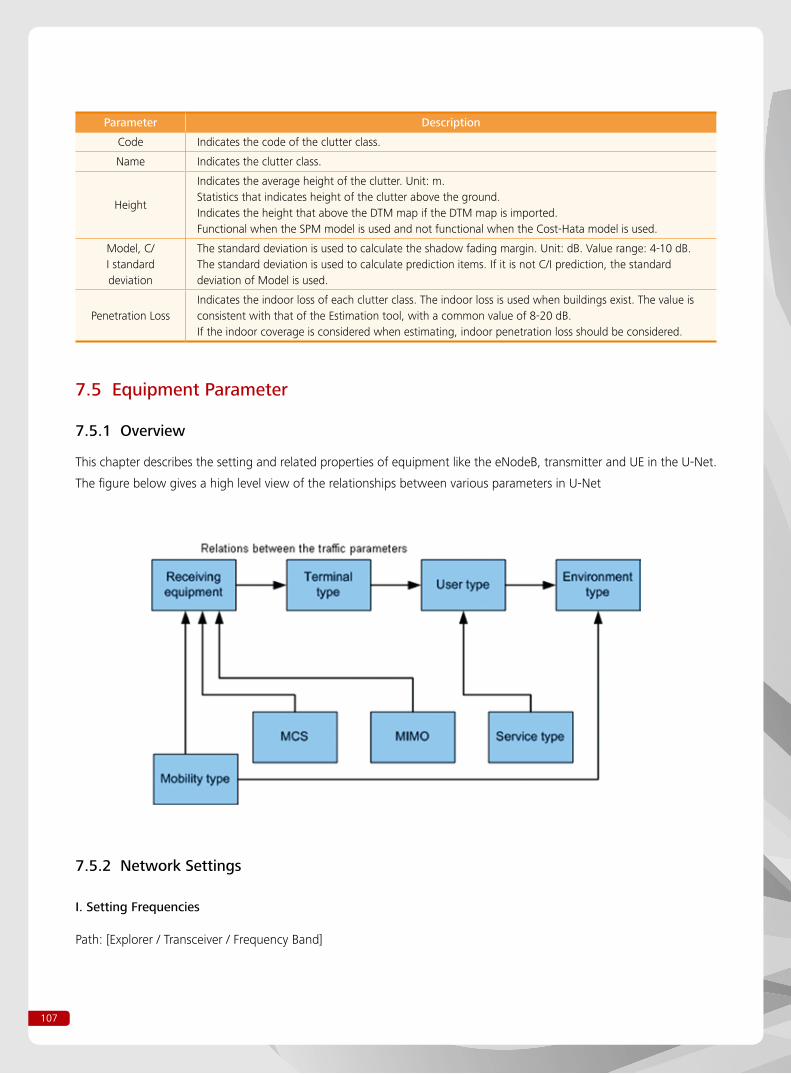
107
Parameter Description
Code Indicates the code of the clutter class.
Name Indicates the clutter class.
Height
Indicates the average height of the clutter. Unit: m.Statistics that indicates height of the clutter above the ground.Indicates the height that above the DTM map if the DTM map is imported.Functional when the SPM model is used and not functional when the Cost-Hata model is used.
Model, C/I standard deviation
The standard deviation is used to calculate the shadow fading margin. Unit: dB. Value range: 4-10 dB.The standard deviation is used to calculate prediction items. If it is not C/I prediction, the standard deviation of Model is used.
Penetration LossIndicates the indoor loss of each clutter class. The indoor loss is used when buildings exist. The value is consistent with that of the Estimation tool, with a common value of 8-20 dB.If the indoor coverage is considered when estimating, indoor penetration loss should be considered.
7.5 Equipment Parameter
7.5.1 Overview
This chapter describes the setting and related properties of equipment like the eNodeB, transmitter and UE in the U-Net.
The figure below gives a high level view of the relationships between various parameters in U-Net
7.5.2 Network Settings
I. Setting Frequencies
Path: [Explorer / Transceiver / Frequency Band]
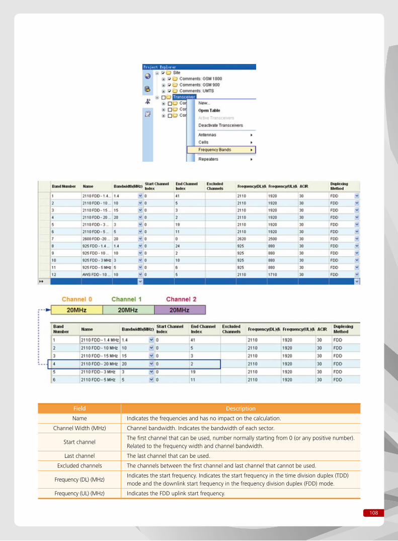
108
Field Description
Name Indicates the frequencies and has no impact on the calculation.
Channel Width (MHz) Channel bandwidth. Indicates the bandwidth of each sector.
Start channelThe first channel that can be used, number normally starting from 0 (or any positive number). Related to the frequency width and channel bandwidth.
Last channel The last channel that can be used.
Excluded channels The channels between the first channel and last channel that cannot be used.
Frequency (DL) (MHz)Indicates the start frequency. Indicates the start frequency in the time division duplex (TDD) mode and the downlink start frequency in the frequency division duplex (FDD) mode.
Frequency (UL) (MHz) Indicates the FDD uplink start frequency.
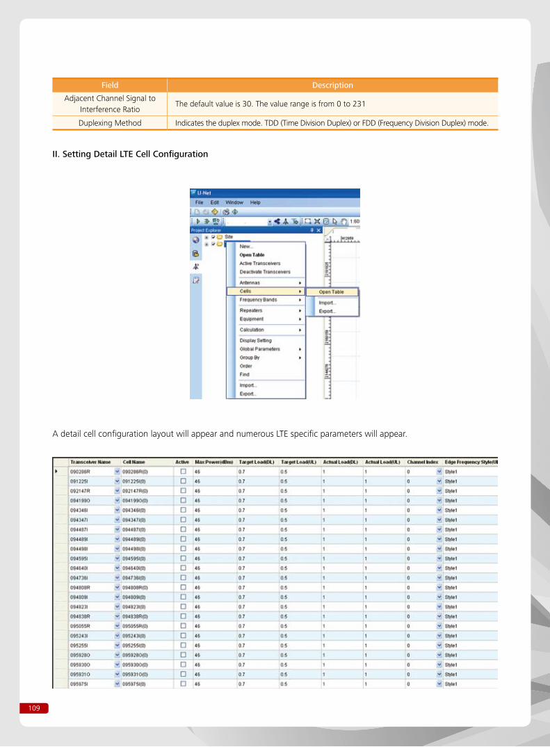
109
Field Description
Adjacent Channel Signal to Interference Ratio
The default value is 30. The value range is from 0 to 231
Duplexing Method Indicates the duplex mode. TDD (Time Division Duplex) or FDD (Frequency Division Duplex) mode.
II. Setting Detail LTE Cell Configuration
A detail cell configuration layout will appear and numerous LTE specific parameters will appear.
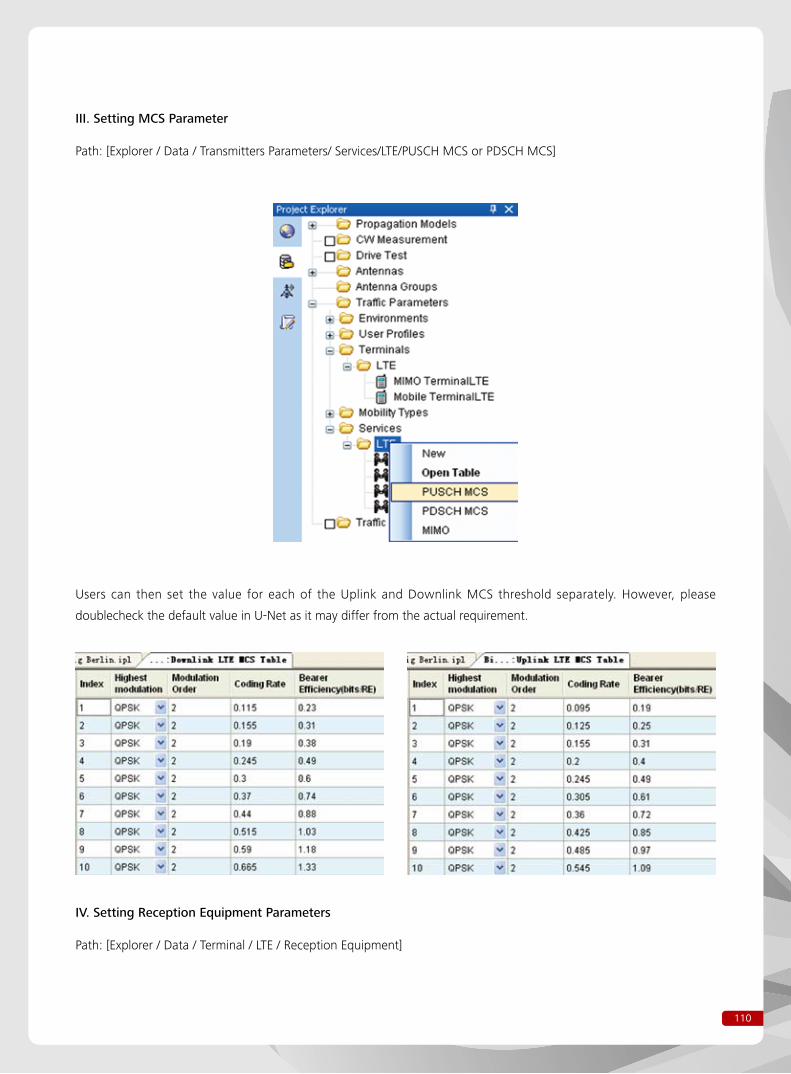
110
III. Setting MCS Parameter
Path: [Explorer / Data / Transmitters Parameters/ Services/LTE/PUSCH MCS or PDSCH MCS]
Users can then set the value for each of the Uplink and Downlink MCS threshold separately. However, please
doublecheck the default value in U-Net as it may differ from the actual requirement.
IV. Setting Reception Equipment Parameters
Path: [Explorer / Data / Terminal / LTE / Reception Equipment]
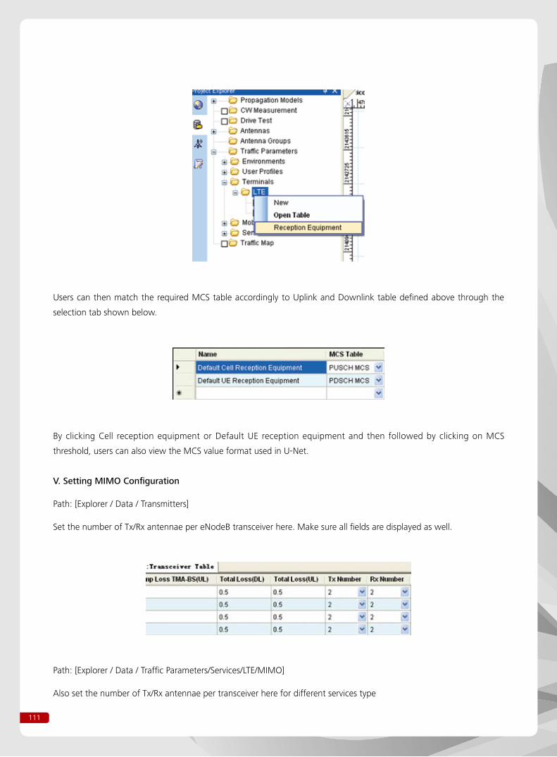
111
Users can then match the required MCS table accordingly to Uplink and Downlink table defined above through the
selection tab shown below.
By clicking Cell reception equipment or Default UE reception equipment and then followed by clicking on MCS
threshold, users can also view the MCS value format used in U-Net.
V. Setting MIMO Configuration
Path: [Explorer / Data / Transmitters]
Set the number of Tx/Rx antennae per eNodeB transceiver here. Make sure all fields are displayed as well.
Path: [Explorer / Data / Traffic Parameters/Services/LTE/MIMO]
Also set the number of Tx/Rx antennae per transceiver here for different services type
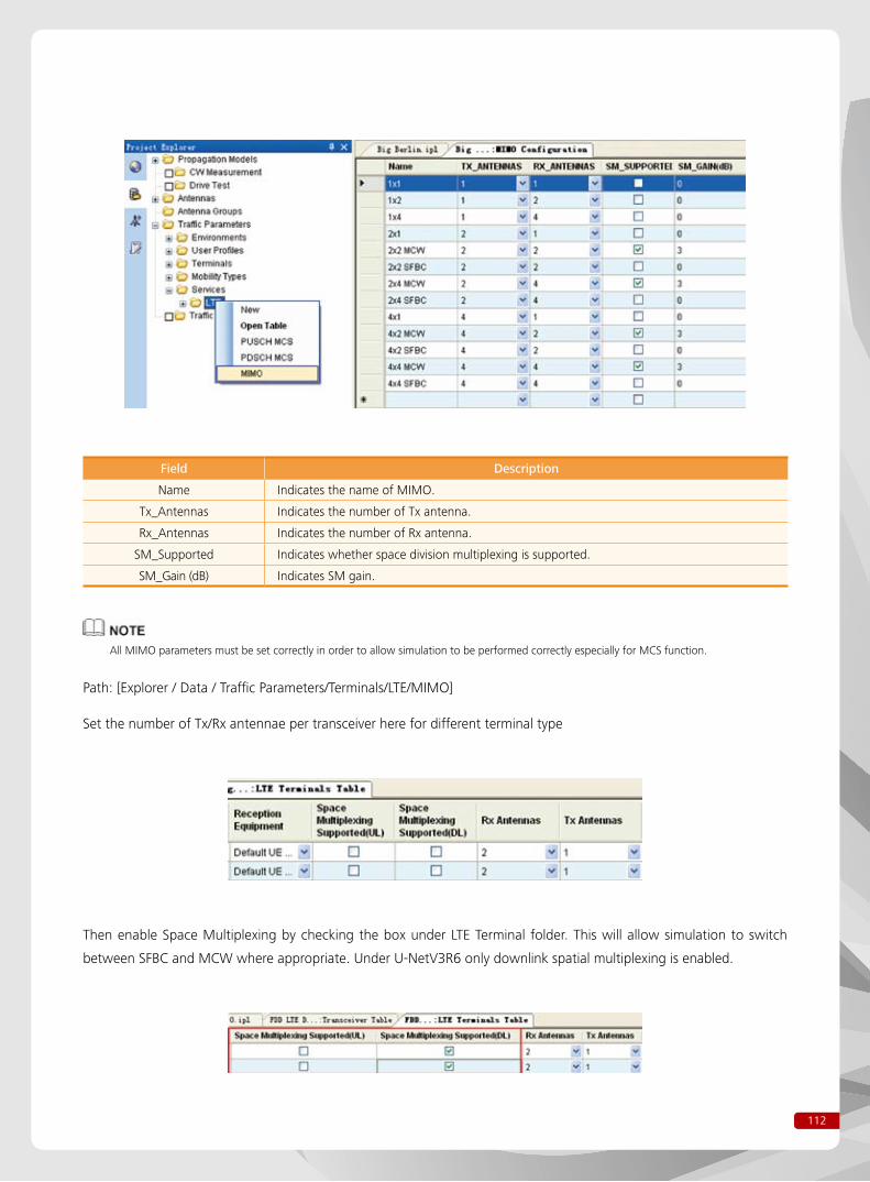
112
Field Description
Name Indicates the name of MIMO.
Tx_Antennas Indicates the number of Tx antenna.
Rx_Antennas Indicates the number of Rx antenna.
SM_Supported Indicates whether space division multiplexing is supported.
SM_Gain (dB) Indicates SM gain.
All MIMO parameters must be set correctly in order to allow simulation to be performed correctly especially for MCS function.
Path: [Explorer / Data / Traffic Parameters/Terminals/LTE/MIMO]
Set the number of Tx/Rx antennae per transceiver here for different terminal type
Then enable Space Multiplexing by checking the box under LTE Terminal folder. This will allow simulation to switch
between SFBC and MCW where appropriate. Under U-NetV3R6 only downlink spatial multiplexing is enabled.
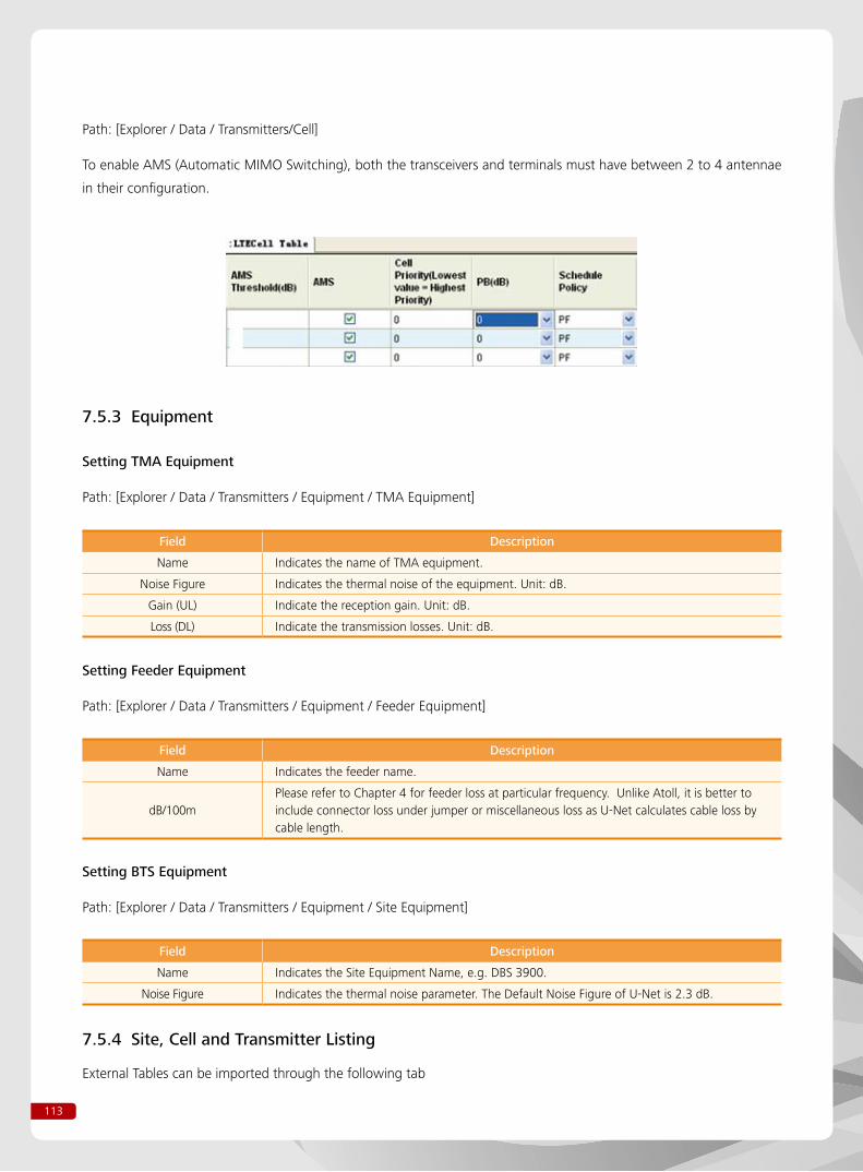
113
Path: [Explorer / Data / Transmitters/Cell]
To enable AMS (Automatic MIMO Switching), both the transceivers and terminals must have between 2 to 4 antennae
in their configuration.
7.5.3 Equipment
Setting TMA Equipment
Path: [Explorer / Data / Transmitters / Equipment / TMA Equipment]
Setting Feeder Equipment
Path: [Explorer / Data / Transmitters / Equipment / Feeder Equipment]
Field Description
Name Indicates the name of TMA equipment.
Noise Figure Indicates the thermal noise of the equipment. Unit: dB.
Gain (UL) Indicate the reception gain. Unit: dB.
Loss (DL) Indicate the transmission losses. Unit: dB.
Field Description
Name Indicates the feeder name.
dB/100mPlease refer to Chapter 4 for feeder loss at particular frequency. Unlike Atoll, it is better to include connector loss under jumper or miscellaneous loss as U-Net calculates cable loss by cable length.
Field Description
Name Indicates the Site Equipment Name, e.g. DBS 3900.
Noise Figure Indicates the thermal noise parameter. The Default Noise Figure of U-Net is 2.3 dB.
Setting BTS Equipment
Path: [Explorer / Data / Transmitters / Equipment / Site Equipment]
7.5.4 Site, Cell and Transmitter Listing
External Tables can be imported through the following tab
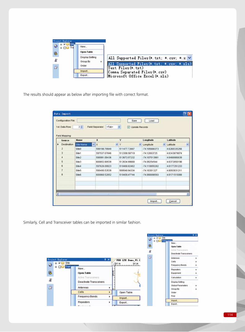
114
The results should appear as below after importing file with correct format.
Similarly, Cell and Transceiver tables can be imported in similar fashion.
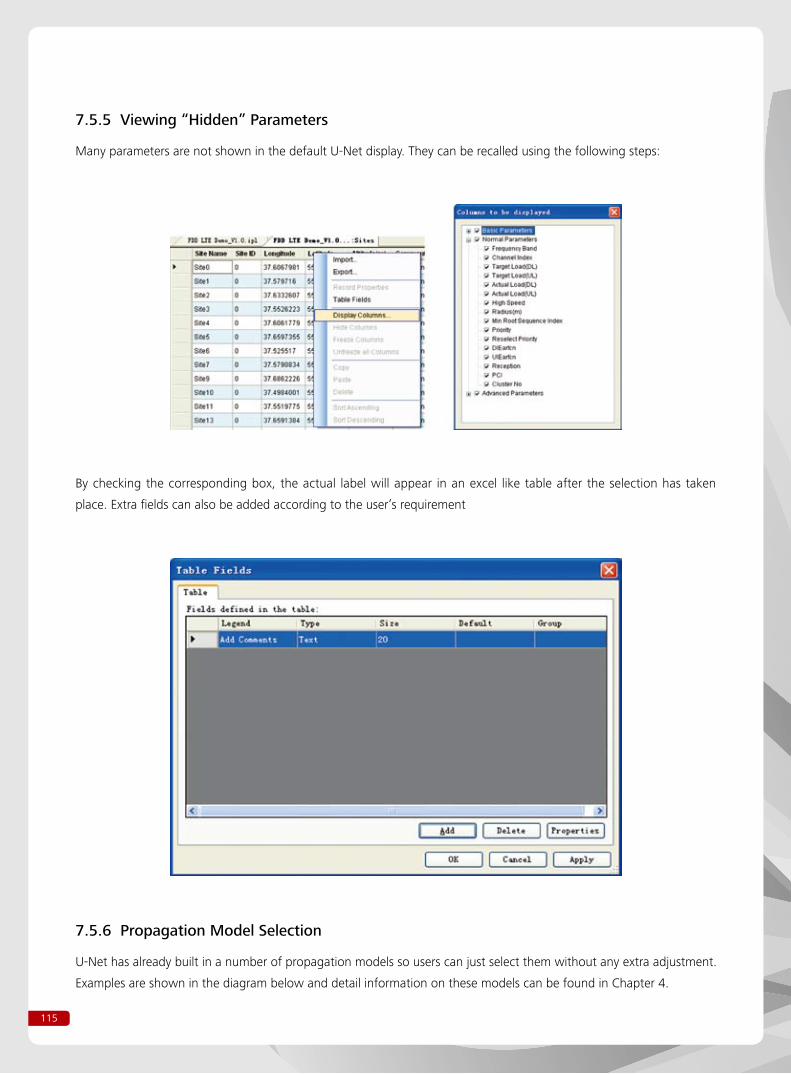
115
7.5.5 Viewing “Hidden” Parameters
Many parameters are not shown in the default U-Net display. They can be recalled using the following steps:
By checking the corresponding box, the actual label will appear in an excel like table after the selection has taken
place. Extra fields can also be added according to the user’s requirement
7.5.6 Propagation Model Selection
U-Net has already built in a number of propagation models so users can just select them without any extra adjustment.
Examples are shown in the diagram below and detail information on these models can be found in Chapter 4.
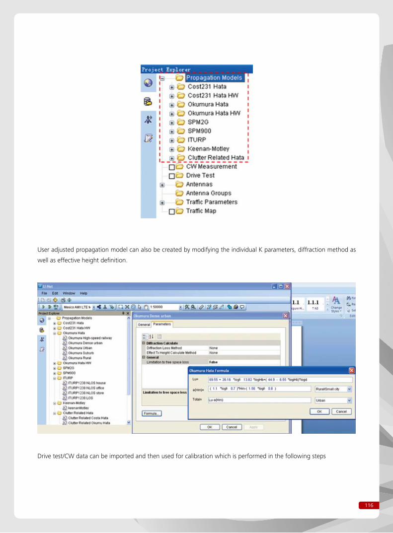
116
User adjusted propagation model can also be created by modifying the individual K parameters, diffraction method as
well as effective height definition.
Drive test/CW data can be imported and then used for calibration which is performed in the following steps
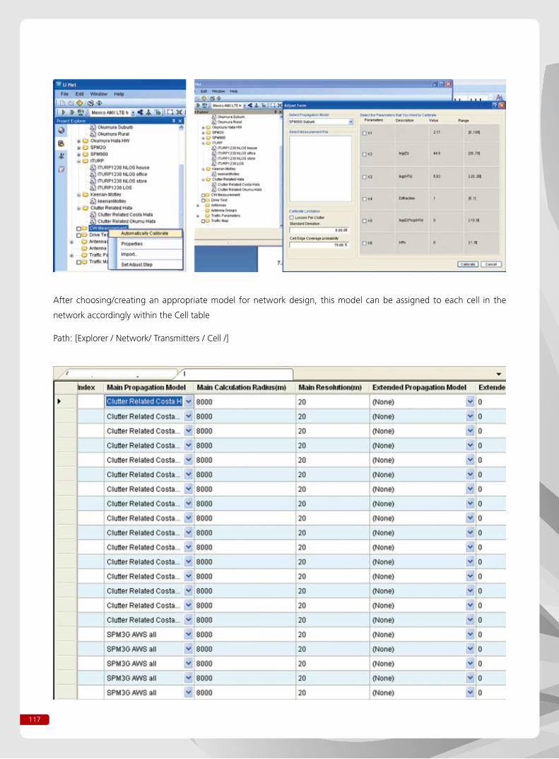
117
After choosing/creating an appropriate model for network design, this model can be assigned to each cell in the
network accordingly within the Cell table
Path: [Explorer / Network/ Transmitters / Cell /]
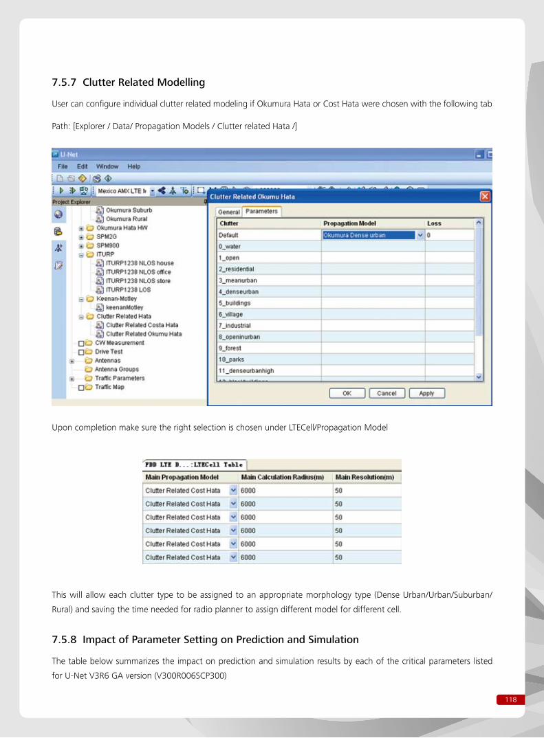
118
7.5.7 Clutter Related Modelling
User can configure individual clutter related modeling if Okumura Hata or Cost Hata were chosen with the following tab
Path: [Explorer / Data/ Propagation Models / Clutter related Hata /]
Upon completion make sure the right selection is chosen under LTECell/Propagation Model
This will allow each clutter type to be assigned to an appropriate morphology type (Dense Urban/Urban/Suburban/
Rural) and saving the time needed for radio planner to assign different model for different cell.
7.5.8 Impact of Parameter Setting on Prediction and Simulation
The table below summarizes the impact on prediction and simulation results by each of the critical parameters listed
for U-Net V3R6 GA version (V300R006SCP300)
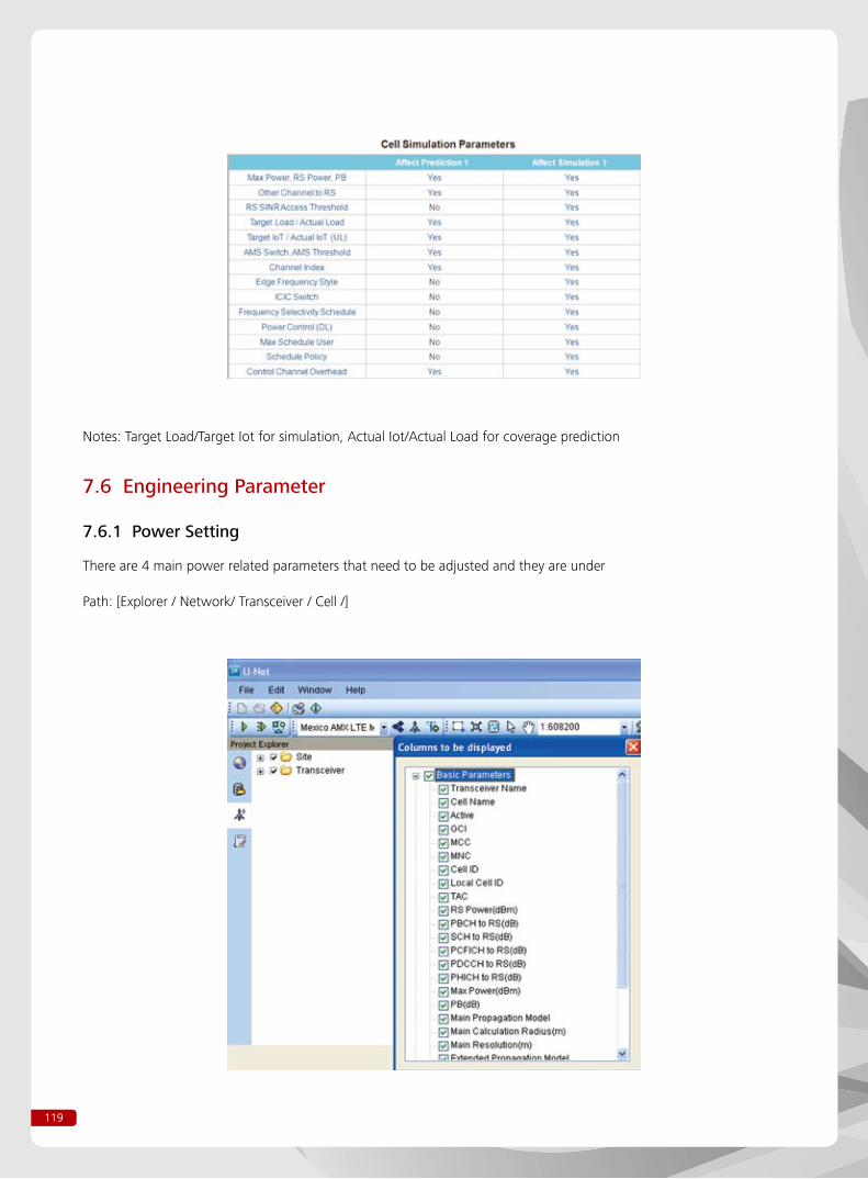
119
Notes: Target Load/Target Iot for simulation, Actual Iot/Actual Load for coverage prediction
7.6 Engineering Parameter
7.6.1 Power Setting
There are 4 main power related parameters that need to be adjusted and they are under
Path: [Explorer / Network/ Transceiver / Cell /]
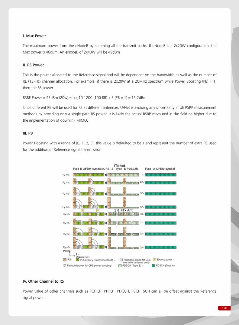
120
I. Max Power
The maximum power from the eNodeB by summing all the transmit paths. If eNodeB is a 2x20W configuration, the
Max power is 46dBm. An eNodeB of 2x40W will be 49dBm
II. RS Power
This is the power allocated to the Reference signal and will be dependent on the bandwidth as well as the number of
RE (15kHz) channel allocation. For example, if there is 2x20W at a 20MHz spectrum while Power Boosting (PB) = 1,
then the RS power
RSRE Power = 43dBm (20w) – Log10 1200 (100 RB) + 3 (PB = 1) = 15.2dBm
Since different RE will be used for RS at different antennae, U-Net is avoiding any uncertainty in UE RSRP measurement
methods by providing only a single path RS power. It is likely the actual RSRP measured in the field be higher due to
the implementation of downlink MIMO.
III. PB
Power Boosting with a range of [0, 1, 2, 3], this value is defaulted to be 1 and represent the number of extra RE used
for the addition of Reference signal transmission.
IV. Other Channel to RS
Power value of other channels such as PCFICH, PHICH, PDCCH, PBCH, SCH can all be offset against the Reference
signal power.
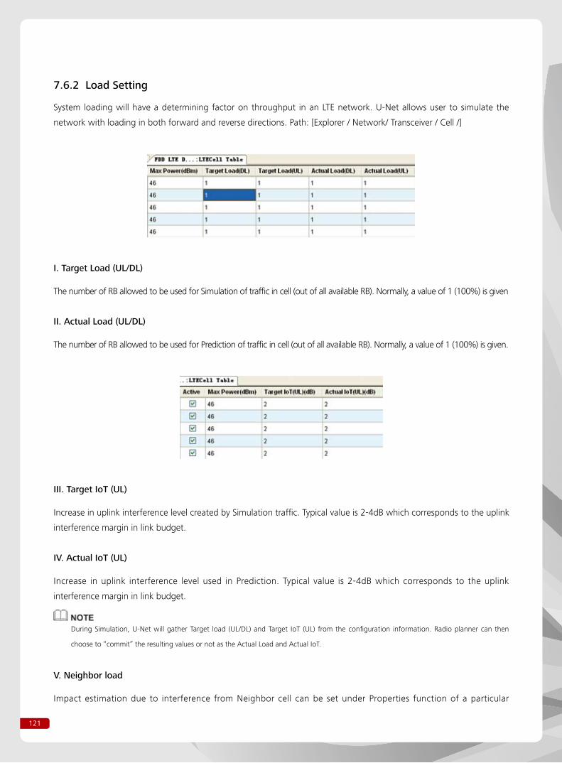
121
7.6.2 Load Setting
System loading will have a determining factor on throughput in an LTE network. U-Net allows user to simulate the
network with loading in both forward and reverse directions. Path: [Explorer / Network/ Transceiver / Cell /]
I. Target Load (UL/DL)
The number of RB allowed to be used for Simulation of traffic in cell (out of all available RB). Normally, a value of 1 (100%) is given
II. Actual Load (UL/DL)
The number of RB allowed to be used for Prediction of traffic in cell (out of all available RB). Normally, a value of 1 (100%) is given.
III. Target IoT (UL)
Increase in uplink interference level created by Simulation traffic. Typical value is 2-4dB which corresponds to the uplink
interference margin in link budget.
IV. Actual IoT (UL)
Increase in uplink interference level used in Prediction. Typical value is 2-4dB which corresponds to the uplink
interference margin in link budget.
During Simulation, U-Net will gather Target load (UL/DL) and Target IoT (UL) from the configuration information. Radio planner can then
choose to “commit” the resulting values or not as the Actual Load and Actual IoT.
V. Neighbor load
Impact estimation due to interference from Neighbor cell can be set under Properties function of a particular
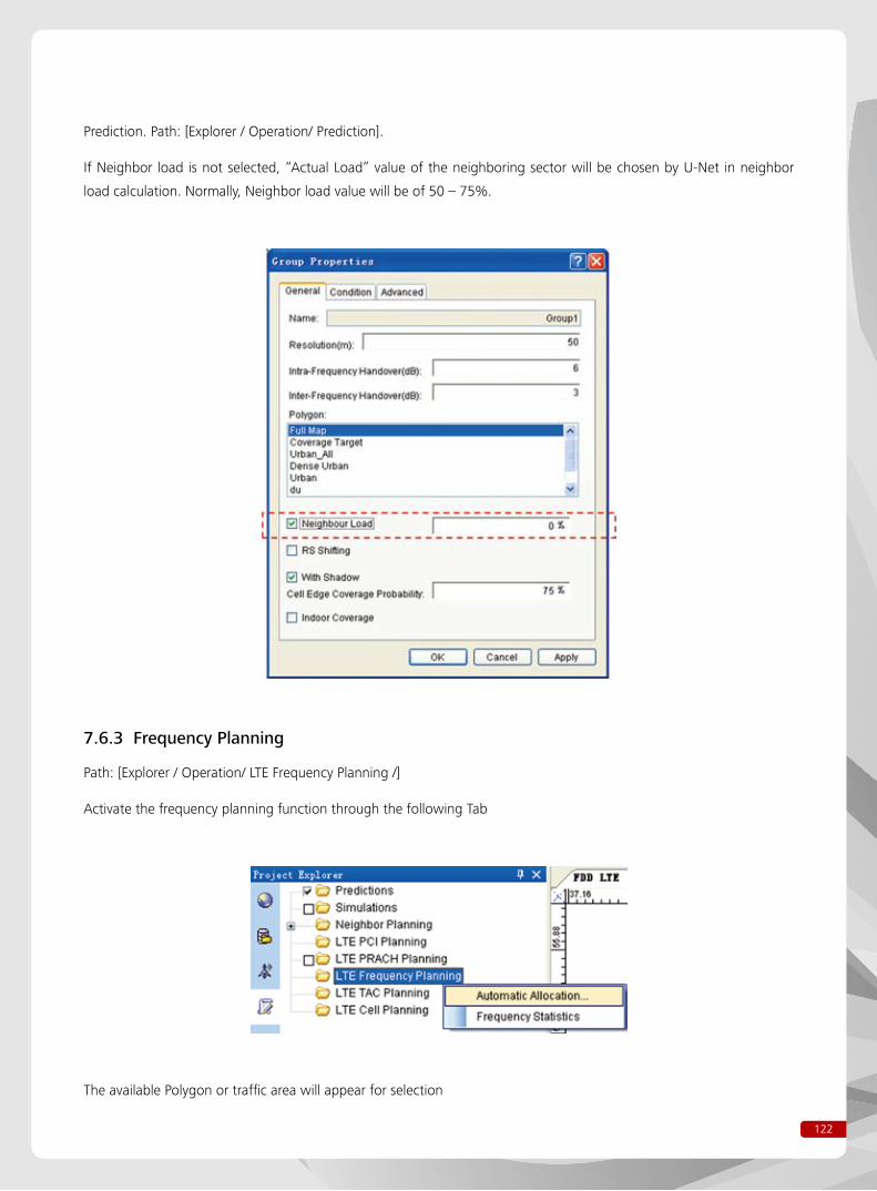
122
Prediction. Path: [Explorer / Operation/ Prediction].
If Neighbor load is not selected, “Actual Load” value of the neighboring sector will be chosen by U-Net in neighbor
load calculation. Normally, Neighbor load value will be of 50 – 75%.
7.6.3 Frequency Planning
Path: [Explorer / Operation/ LTE Frequency Planning /]
Activate the frequency planning function through the following Tab
The available Polygon or traffic area will appear for selection
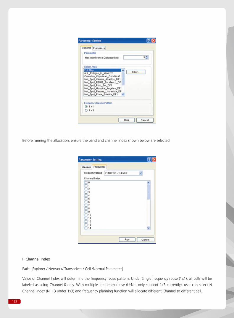
123
Before running the allocation, ensure the band and channel index shown below are selected
I. Channel Index
Path: [Explorer / Network/ Transceiver / Cell /Normal Parameter]
Value of Channel Index will determine the frequency reuse pattern. Under Single frequency reuse (1x1), all cells will be
labeled as using Channel 0 only. With multiple frequency reuse (U-Net only support 1x3 currently), user can select N
Channel index (N = 3 under 1x3) and frequency planning function will allocate different Channel to different cell.
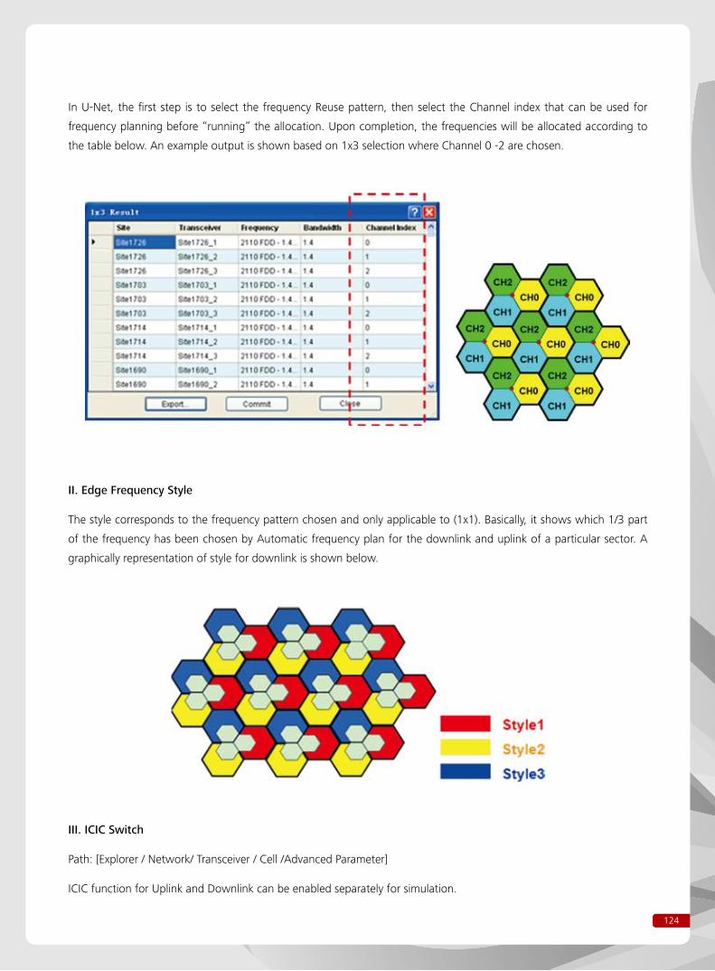
124
In U-Net, the first step is to select the frequency Reuse pattern, then select the Channel index that can be used for
frequency planning before “running” the allocation. Upon completion, the frequencies will be allocated according to
the table below. An example output is shown based on 1x3 selection where Channel 0 -2 are chosen.
II. Edge Frequency Style
The style corresponds to the frequency pattern chosen and only applicable to (1x1). Basically, it shows which 1/3 part
of the frequency has been chosen by Automatic frequency plan for the downlink and uplink of a particular sector. A
graphically representation of style for downlink is shown below.
III. ICIC Switch
Path: [Explorer / Network/ Transceiver / Cell /Advanced Parameter]
ICIC function for Uplink and Downlink can be enabled separately for simulation.
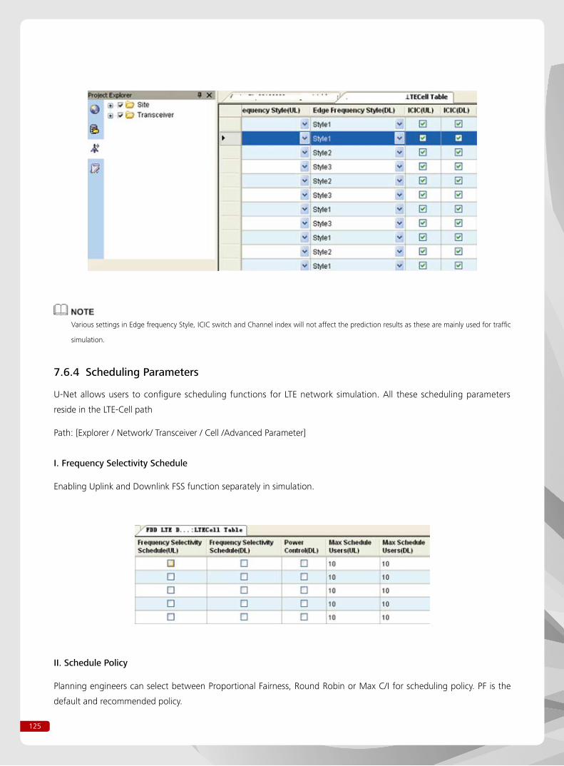
125
Various settings in Edge frequency Style, ICIC switch and Channel index will not affect the prediction results as these are mainly used for traffic
simulation.
7.6.4 Scheduling Parameters
U-Net allows users to configure scheduling functions for LTE network simulation. All these scheduling parameters
reside in the LTE-Cell path
Path: [Explorer / Network/ Transceiver / Cell /Advanced Parameter]
I. Frequency Selectivity Schedule
Enabling Uplink and Downlink FSS function separately in simulation.
II. Schedule Policy
Planning engineers can select between Proportional Fairness, Round Robin or Max C/I for scheduling policy. PF is the
default and recommended policy.
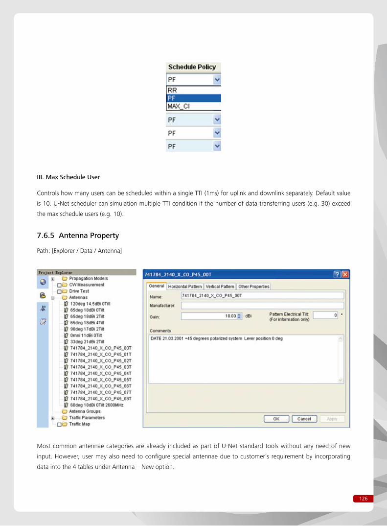
126
III. Max Schedule User
Controls how many users can be scheduled within a single TTI (1ms) for uplink and downlink separately. Default value
is 10. U-Net scheduler can simulation multiple TTI condition if the number of data transferring users (e.g. 30) exceed
the max schedule users (e.g. 10).
7.6.5 Antenna Property
Path: [Explorer / Data / Antenna]
Most common antennae categories are already included as part of U-Net standard tools without any need of new
input. However, user may also need to configure special antennae due to customer’s requirement by incorporating
data into the 4 tables under Antenna – New option.
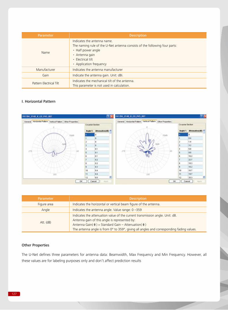
127
Parameter Description
Name
Indicates the antenna name.The naming rule of the U-Net antenna consists of the following four parts:
Half power angle• Antenna gain• Electrical tilt• Application frequency•
Manufacturer Indicates the antenna manufacturer
Gain Indicate the antenna gain. Unit: dBi.
Pattern Electrical TiltIndicates the mechanical tilt of the antenna.This parameter is not used in calculation.
Parameter Description
Figure area Indicates the horizontal or vertical beam figure of the antenna.
Angle Indicates the antenna angle. Value range: 0 –359
Att. (dB)
Indicates the attenuation value of the current transmission angle. Unit: dB.Antenna gain of this angle is represented by:Antenna Gain(θ) = Standard Gain – Attenuation(θ)The antenna angle is from 0° to 359°, giving all angles and corresponding fading values.
I. Horizontal Pattern
Other Properties
The U-Net defines three parameters for antenna data: Beamwidth, Max Frequency and Min Frequency. However, all
these values are for labeling purposes only and don’t affect prediction results
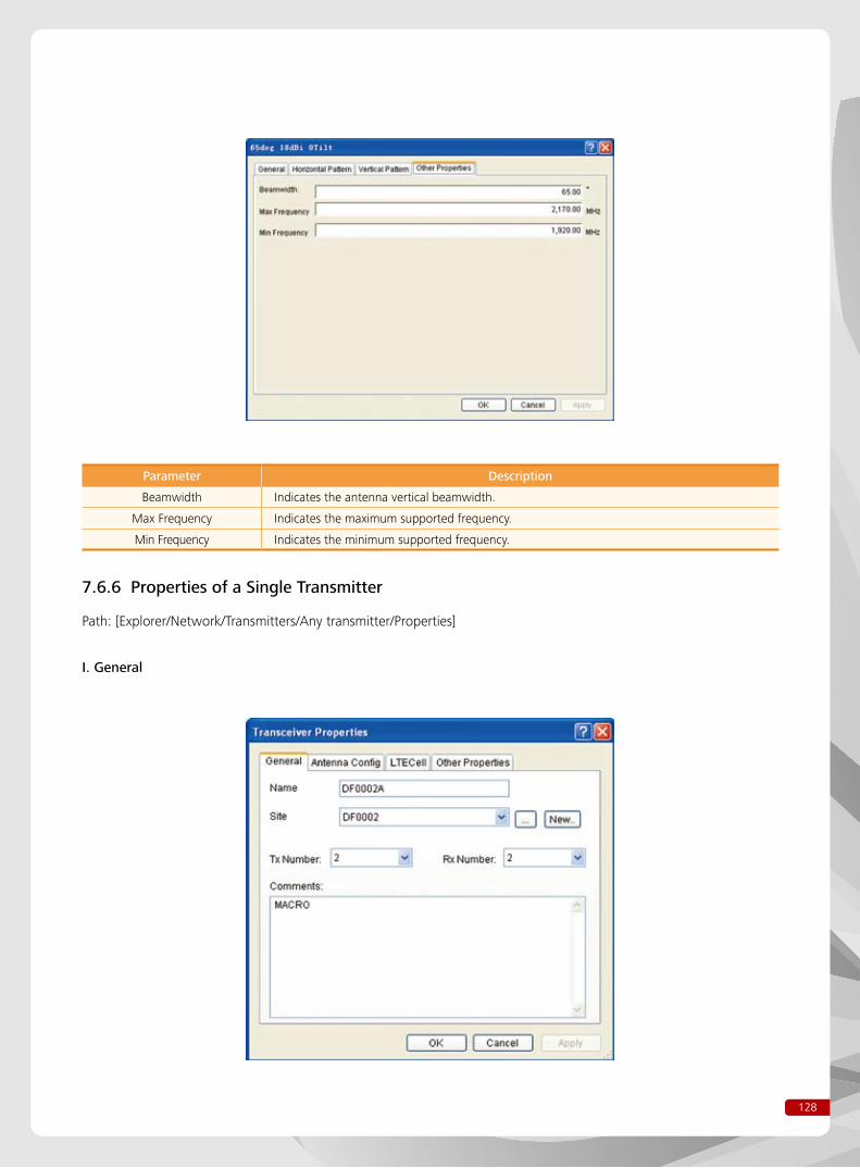
128
Parameter Description
Beamwidth Indicates the antenna vertical beamwidth.
Max Frequency Indicates the maximum supported frequency.
Min Frequency Indicates the minimum supported frequency.
7.6.6 Properties of a Single Transmitter
Path: [Explorer/Network/Transmitters/Any transmitter/Properties]
I. General
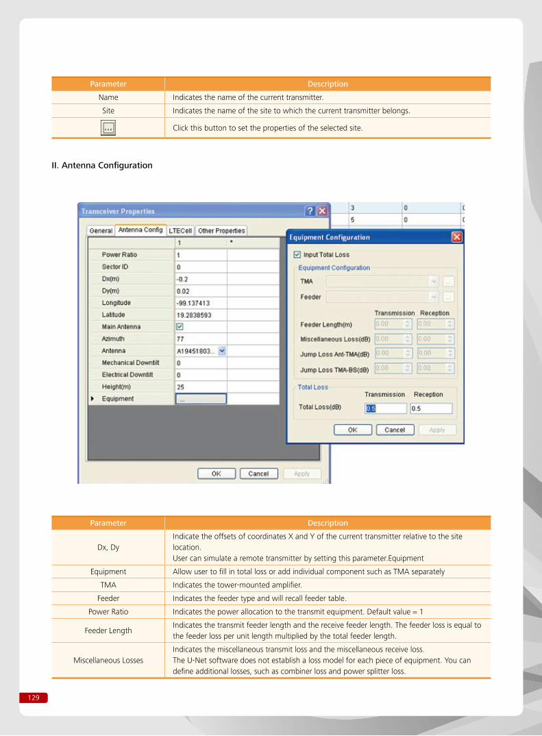
129
Parameter Description
Name Indicates the name of the current transmitter.
Site Indicates the name of the site to which the current transmitter belongs.
Click this button to set the properties of the selected site.
II. Antenna Configuration
Parameter Description
Dx, DyIndicate the offsets of coordinates X and Y of the current transmitter relative to the site location.User can simulate a remote transmitter by setting this parameter.Equipment
Equipment Allow user to fill in total loss or add individual component such as TMA separately
TMA Indicates the tower-mounted amplifier.
Feeder Indicates the feeder type and will recall feeder table.
Power Ratio Indicates the power allocation to the transmit equipment. Default value = 1
Feeder LengthIndicates the transmit feeder length and the receive feeder length. The feeder loss is equal to the feeder loss per unit length multiplied by the total feeder length.
Miscellaneous LossesIndicates the miscellaneous transmit loss and the miscellaneous receive loss.The U-Net software does not establish a loss model for each piece of equipment. You can define additional losses, such as combiner loss and power splitter loss.
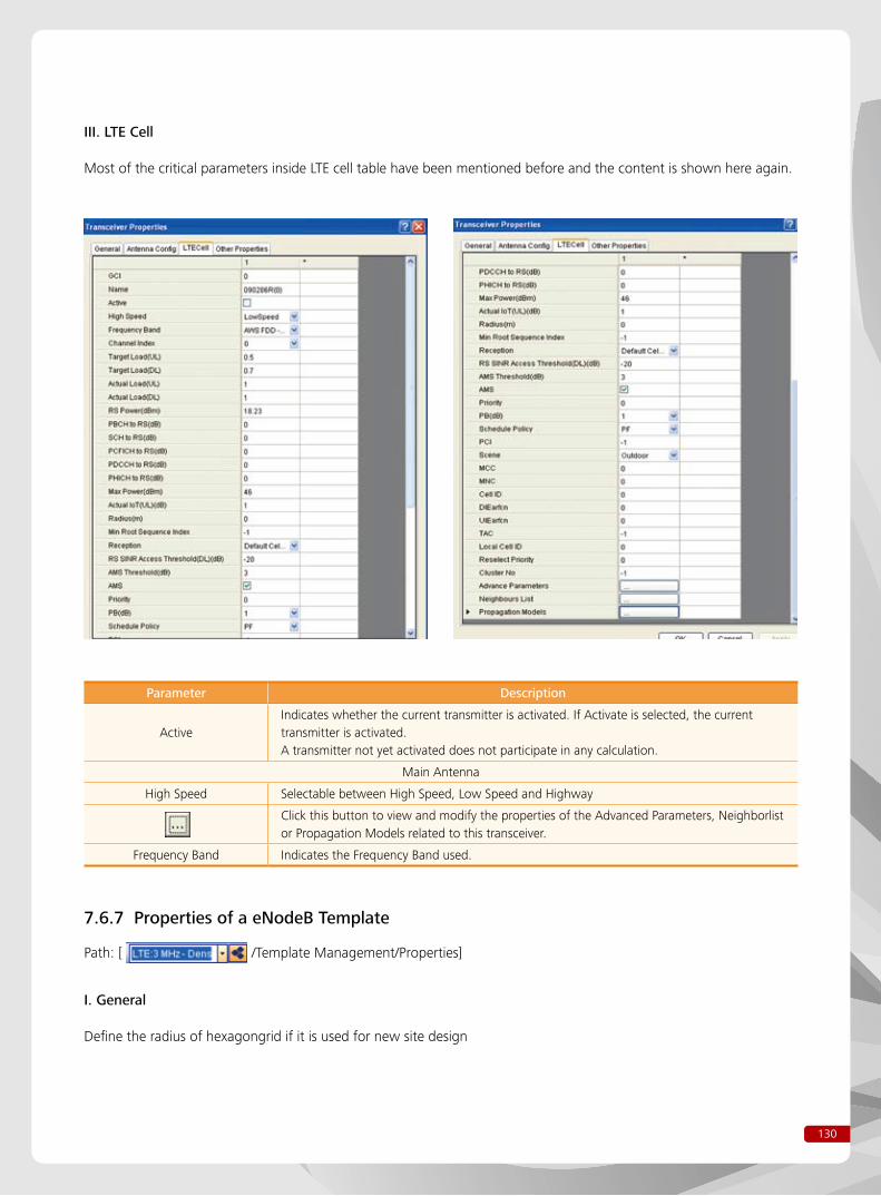
130
III. LTE Cell
Most of the critical parameters inside LTE cell table have been mentioned before and the content is shown here again.
Parameter Description
ActiveIndicates whether the current transmitter is activated. If Activate is selected, the current transmitter is activated.A transmitter not yet activated does not participate in any calculation.
Main Antenna
High Speed Selectable between High Speed, Low Speed and Highway
Click this button to view and modify the properties of the Advanced Parameters, Neighborlist or Propagation Models related to this transceiver.
Frequency Band Indicates the Frequency Band used.
7.6.7 Properties of a eNodeB Template
Path: [ /Template Management/Properties]
I. General
Define the radius of hexagongrid if it is used for new site design
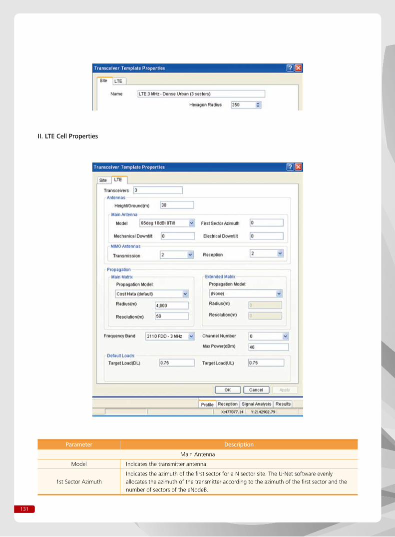
131
II. LTE Cell Properties
Parameter Description
Main Antenna
Model Indicates the transmitter antenna.
1st Sector AzimuthIndicates the azimuth of the first sector for a N sector site. The U-Net software evenly allocates the azimuth of the transmitter according to the azimuth of the first sector and the number of sectors of the eNodeB.
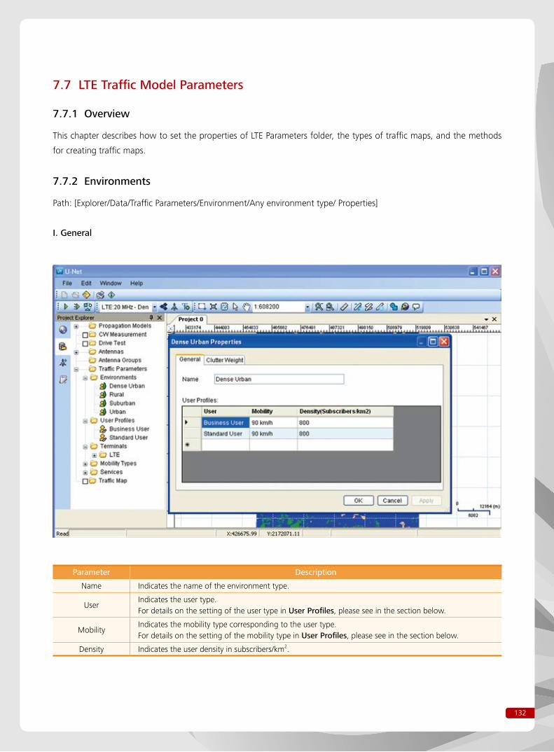
132
7.7 LTE Traffic Model Parameters
7.7.1 Overview
This chapter describes how to set the properties of LTE Parameters folder, the types of traffic maps, and the methods
for creating traffic maps.
7.7.2 Environments
Path: [Explorer/Data/Traffic Parameters/Environment/Any environment type/ Properties]
I. General
Parameter Description
Name Indicates the name of the environment type.
UserIndicates the user type. For details on the setting of the user type in User Profiles, please see in the section below.
MobilityIndicates the mobility type corresponding to the user type. For details on the setting of the mobility type in User Profiles, please see in the section below.
Density Indicates the user density in subscribers/km2.
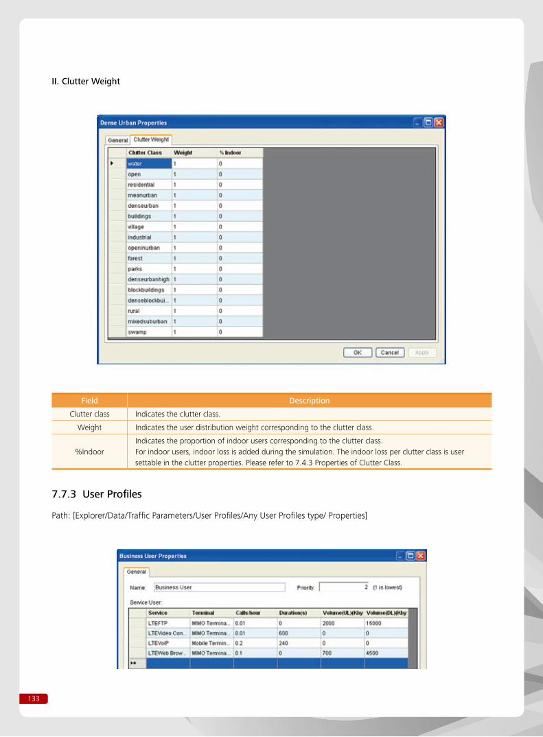
133
II. Clutter Weight
Field Description
Clutter class Indicates the clutter class.
Weight Indicates the user distribution weight corresponding to the clutter class.
%IndoorIndicates the proportion of indoor users corresponding to the clutter class.For indoor users, indoor loss is added during the simulation. The indoor loss per clutter class is user settable in the clutter properties. Please refer to 7.4.3 Properties of Clutter Class.
7.7.3 User Profiles
Path: [Explorer/Data/Traffic Parameters/User Profiles/Any User Profiles type/ Properties]
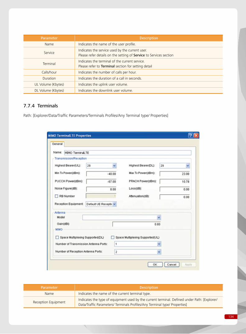
134
Parameter Description
Name Indicates the name of the user profile.
ServiceIndicates the service used by the current user.Please refer details on the setting of Service to Services section
TerminalIndicates the terminal of the current service.Please refer to Terminal section for setting detail
Calls/hour Indicates the number of calls per hour.
Duration Indicates the duration of a call in seconds.
UL Volume (Kbytes) Indicates the uplink user volume.
DL Volume (Kbytes) Indicates the downlink user volume.
Parameter Description
Name Indicates the name of the current terminal type.
Reception EquipmentIndicates the type of equipment used by the current terminal. Defined under Path: [Explorer/Data/Traffic Parameters/ Terminals Profiles/Any Terminal type/ Properties]
7.7.4 Terminals
Path: [Explorer/Data/Traffic Parameters/Terminals Profiles/Any Terminal type/ Properties]
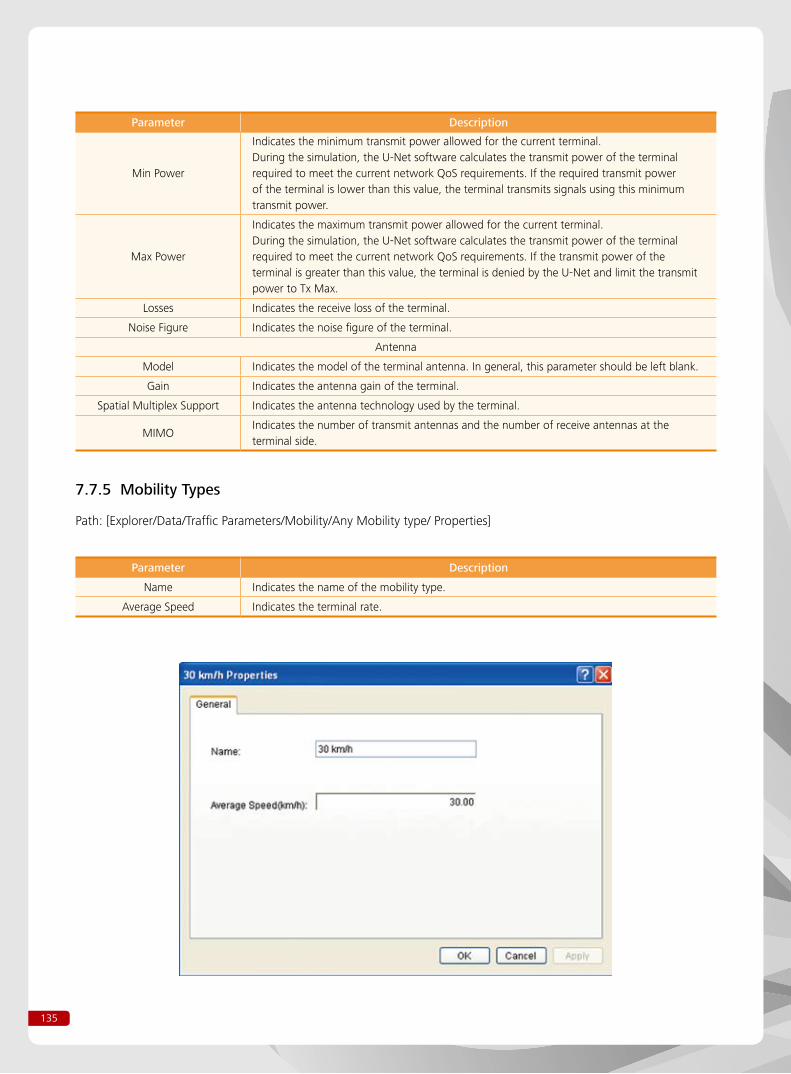
135
Parameter Description
Min Power
Indicates the minimum transmit power allowed for the current terminal.During the simulation, the U-Net software calculates the transmit power of the terminal required to meet the current network QoS requirements. If the required transmit power of the terminal is lower than this value, the terminal transmits signals using this minimum transmit power.
Max Power
Indicates the maximum transmit power allowed for the current terminal. During the simulation, the U-Net software calculates the transmit power of the terminal required to meet the current network QoS requirements. If the transmit power of the terminal is greater than this value, the terminal is denied by the U-Net and limit the transmit power to Tx Max.
Losses Indicates the receive loss of the terminal.
Noise Figure Indicates the noise figure of the terminal.
Antenna
Model Indicates the model of the terminal antenna. In general, this parameter should be left blank.
Gain Indicates the antenna gain of the terminal.
Spatial Multiplex Support Indicates the antenna technology used by the terminal.
MIMOIndicates the number of transmit antennas and the number of receive antennas at the terminal side.
Parameter Description
Name Indicates the name of the mobility type.
Average Speed Indicates the terminal rate.
7.7.5 Mobility Types
Path: [Explorer/Data/Traffic Parameters/Mobility/Any Mobility type/ Properties]
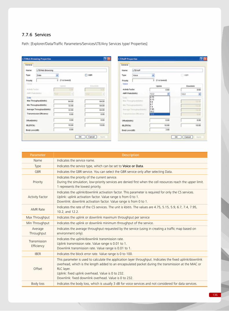
136
Parameter Description
Name Indicates the service name.
Type Indicates the service type, which can be set to Voice or Data.
GBR Indicates the GBR service. You can select the GBR service only after selecting Data.
PriorityIndicates the priority of the current service.During the simulation, low-priority services are denied first when the cell resources reach the upper limit.1 represents the lowest priority.
Activity FactorIndicates the uplink/downlink activation factor. This parameter is required for only the CS services.Uplink: uplink activation factor. Value range is from 0 to 1.Downlink: downlink activation factor. Value range is from 0 to 1.
AMR RateIndicates the rate of the CS services. The unit is kbit/s. The values are 4.75, 5.15, 5.9, 6.7, 7.4, 7.95, 10.2, and 12.2.
Max Throughput Indicates the uplink or downlink maximum throughput per service
Min Throughput Indicates the uplink or downlink minimum throughput of the service.
Average Throughput
Indicates the average throughput requested by the service (using in creating a traffic map based on environment only).
Transmission Efficiency
Indicates the uplink/downlink transmission rate.Uplink transmission rate. Value range is 0.01 to 1.Downlink transmission rate. Value range is 0.01 to 1.
IBER Indicates the block error rate. Value range is 0 to 100.
Offset
This parameter is used to calculate the application layer throughput. Indicates the fixed uplink/downlink overhead, which is the length added to an encapsulated packet during the transmission at the MAC or RLC layer.Uplink: fixed uplink overhead. Value is 0 to 232.Downlink: fixed downlink overhead. Value is 0 to 232.
Body loss Indicates the body loss, which is usually 3 dB for voice services and not considered for data services.
7.7.6 Services
Path: [Explorer/Data/Traffic Parameters/Services/LTE/Any Services type/ Properties]
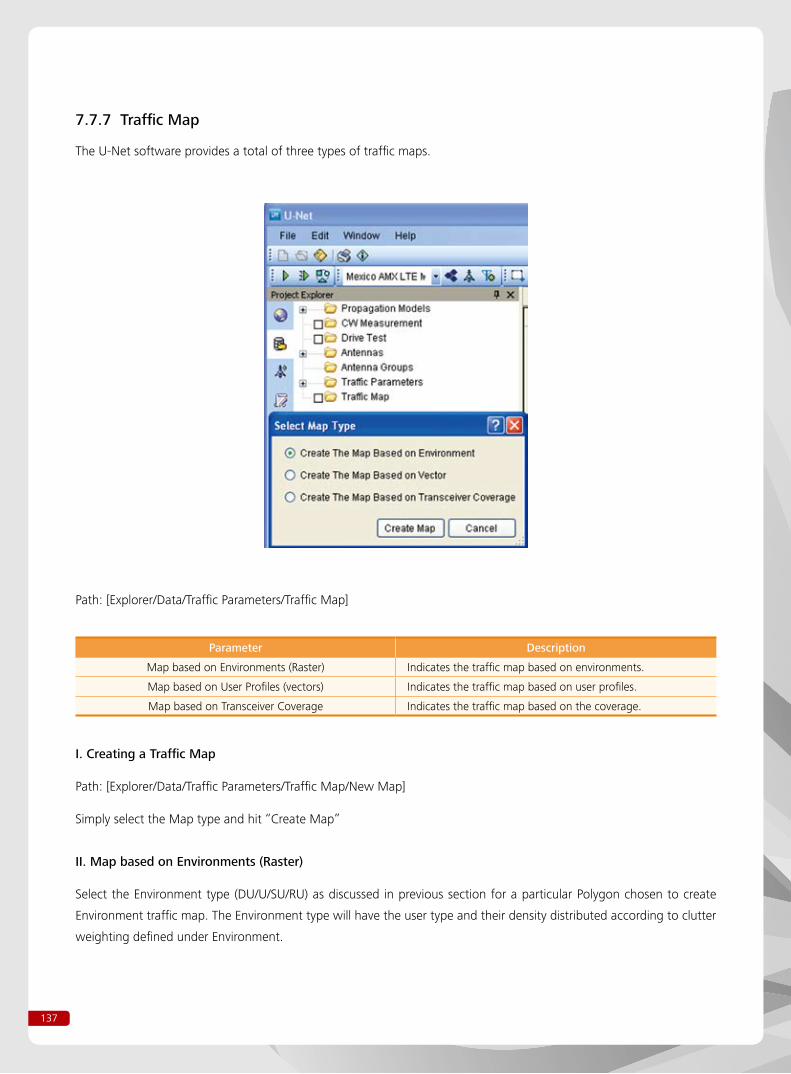
137
7.7.7 Traffic Map
The U-Net software provides a total of three types of traffic maps.
Path: [Explorer/Data/Traffic Parameters/Traffic Map]
Parameter Description
Map based on Environments (Raster) Indicates the traffic map based on environments.
Map based on User Profiles (vectors) Indicates the traffic map based on user profiles.
Map based on Transceiver Coverage Indicates the traffic map based on the coverage.
I. Creating a Traffic Map
Path: [Explorer/Data/Traffic Parameters/Traffic Map/New Map]
Simply select the Map type and hit “Create Map”
II. Map based on Environments (Raster)
Select the Environment type (DU/U/SU/RU) as discussed in previous section for a particular Polygon chosen to create
Environment traffic map. The Environment type will have the user type and their density distributed according to clutter
weighting defined under Environment.
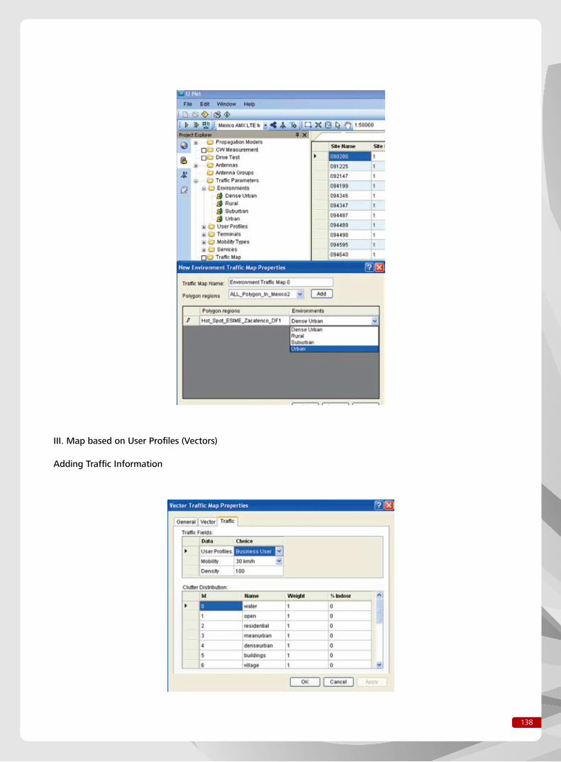
138
III. Map based on User Profiles (Vectors)
Adding Traffic Information
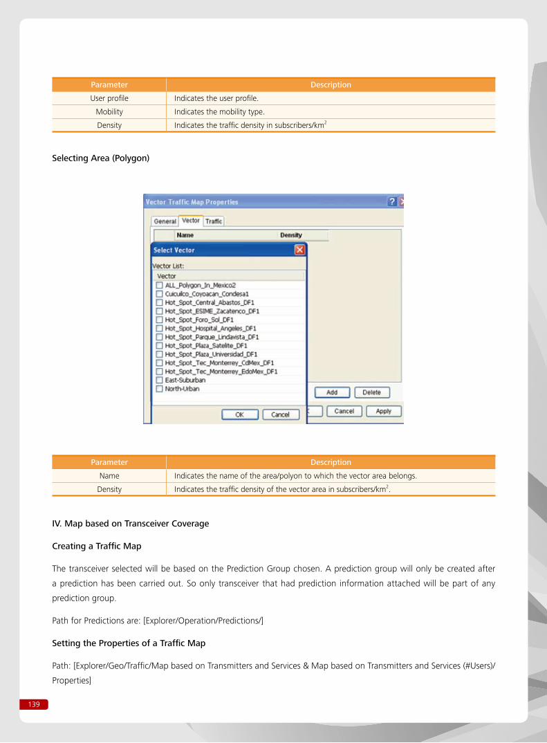
139
Selecting Area (Polygon)
Parameter Description
User profile Indicates the user profile.
Mobility Indicates the mobility type.
Density Indicates the traffic density in subscribers/km2
Parameter Description
Name Indicates the name of the area/polyon to which the vector area belongs.
Density Indicates the traffic density of the vector area in subscribers/km2.
IV. Map based on Transceiver Coverage
Creating a Traffic Map
The transceiver selected will be based on the Prediction Group chosen. A prediction group will only be created after
a prediction has been carried out. So only transceiver that had prediction information attached will be part of any
prediction group.
Path for Predictions are: [Explorer/Operation/Predictions/]
Setting the Properties of a Traffic Map
Path: [Explorer/Geo/Traffic/Map based on Transmitters and Services & Map based on Transmitters and Services (#Users)/
Properties]
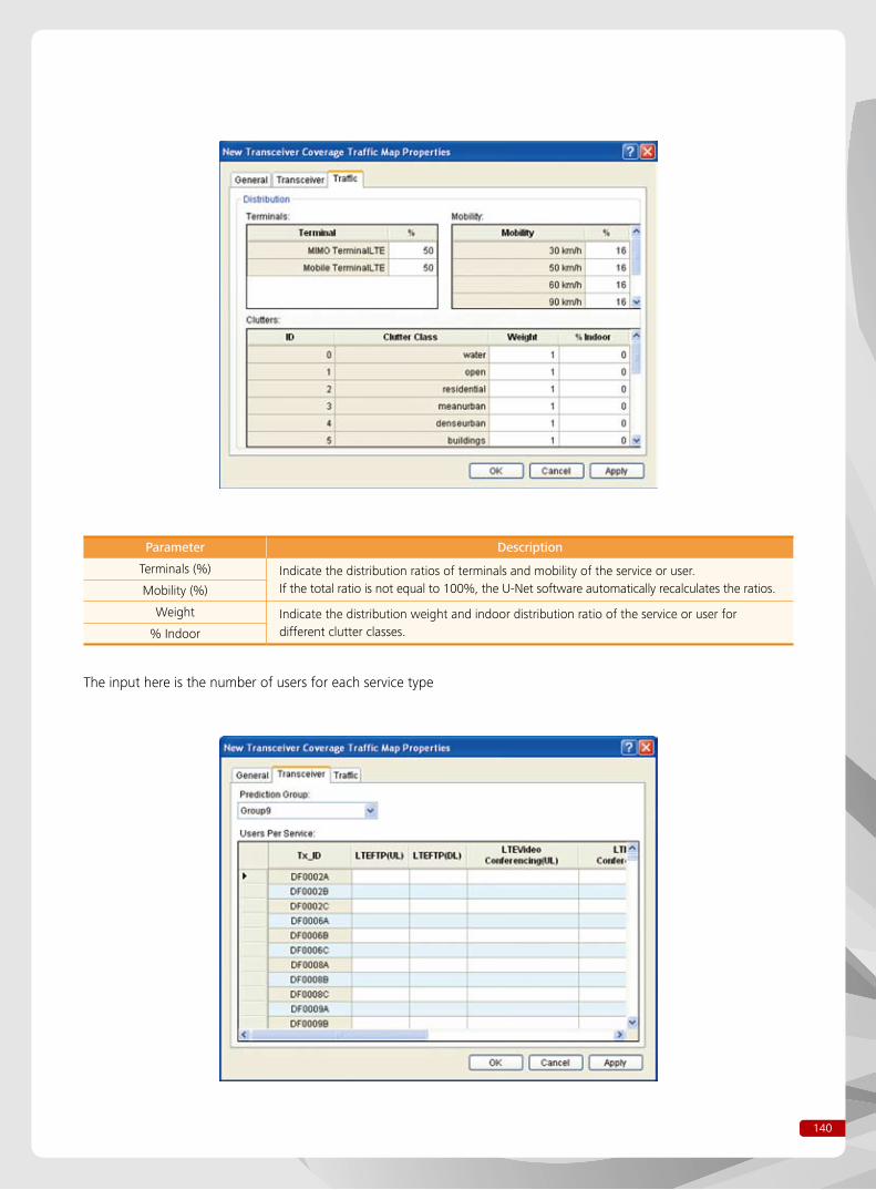
140
Parameter Description
Terminals (%) Indicate the distribution ratios of terminals and mobility of the service or user.If the total ratio is not equal to 100%, the U-Net software automatically recalculates the ratios.Mobility (%)
Weight Indicate the distribution weight and indoor distribution ratio of the service or user for different clutter classes.% Indoor
The input here is the number of users for each service type
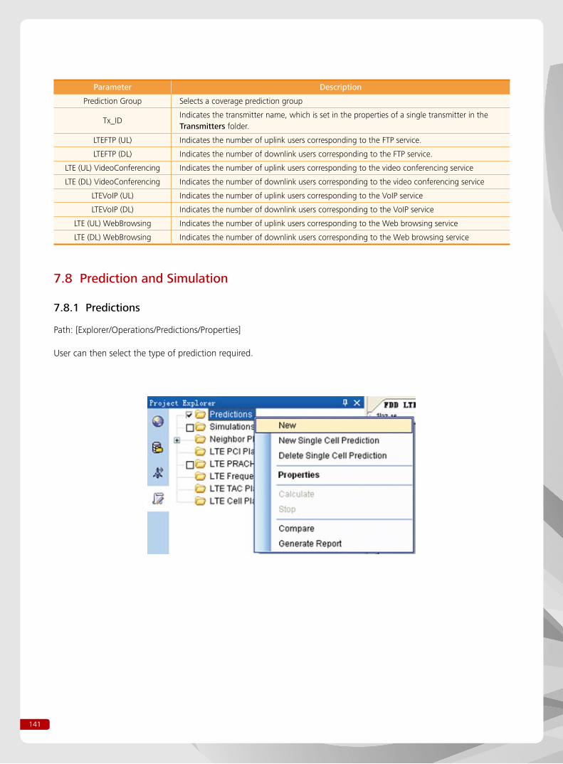
141
7.8 Prediction and Simulation
7.8.1 Predictions
Path: [Explorer/Operations/Predictions/Properties]
User can then select the type of prediction required.
Parameter Description
Prediction Group Selects a coverage prediction group
Tx_IDIndicates the transmitter name, which is set in the properties of a single transmitter in the Transmitters folder.
LTEFTP (UL) Indicates the number of uplink users corresponding to the FTP service.
LTEFTP (DL) Indicates the number of downlink users corresponding to the FTP service.
LTE (UL) VideoConferencing Indicates the number of uplink users corresponding to the video conferencing service
LTE (DL) VideoConferencing Indicates the number of downlink users corresponding to the video conferencing service
LTEVoIP (UL) Indicates the number of uplink users corresponding to the VoIP service
LTEVoIP (DL) Indicates the number of downlink users corresponding to the VoIP service
LTE (UL) WebBrowsing Indicates the number of uplink users corresponding to the Web browsing service
LTE (DL) WebBrowsing Indicates the number of downlink users corresponding to the Web browsing service
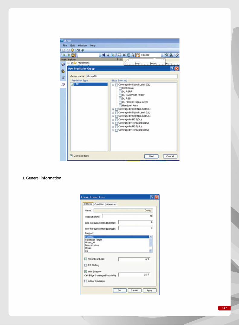
142
I. General information
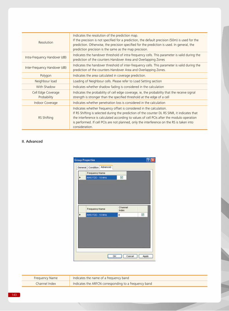
143
II. Advanced
Resolution
Indicates the resolution of the prediction map. If the precision is not specified for a prediction, the default precision (50m) is used for the prediction. Otherwise, the precision specified for the prediction is used. In general, the prediction precision is the same as the map precision.
Intra-Frequency Handover (dB)Indicates the handover threshold of intra-frequency cells. This parameter is valid during the prediction of the counters Handover Area and Overlapping Zones
Inter-Frequency Handover (dB)Indicates the handover threshold of inter-frequency cells. This parameter is valid during the prediction of the counters Handover Area and Overlapping Zones.
Polygon Indicates the area calculated in coverage prediction.
Neighbour load Loading of Neighbour cells. Please refer to Load Setting section
With Shadow Indicates whether shadow fading is considered in the calculation
Cell Edge Coverage Probability
Indicates the probability of cell edge coverage, ie, the probability that the receive signal strength is stronger than the specified threshold at the edge of a cell
Indoor Coverage Indicates whether penetration loss is considered in the calculation
RS Shifting
Indicates whether frequency offset is considered in the calculation. If RS Shifting is selected during the prediction of the counter DL RS SINR, it indicates that the interference is calculated according to values of cell PCIs after the modulo operation is performed. If cell PCIs are not planned, only the interference on the RS is taken into consideration.
Frequency Name Indicates the name of a frequency band
Channel Index Indicates the ARFCN corresponding to a frequency band
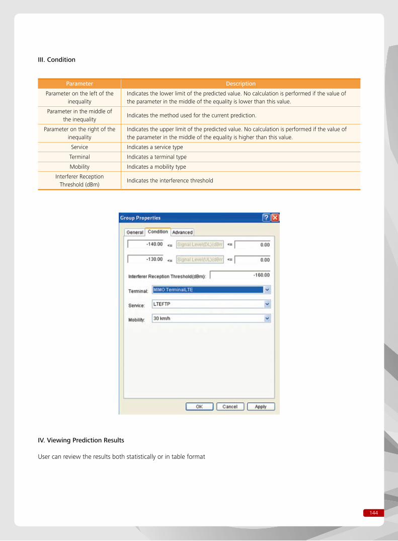
144
III. Condition
Parameter Description
Parameter on the left of the inequality
Indicates the lower limit of the predicted value. No calculation is performed if the value of the parameter in the middle of the equality is lower than this value.
Parameter in the middle of the inequality
Indicates the method used for the current prediction.
Parameter on the right of the inequality
Indicates the upper limit of the predicted value. No calculation is performed if the value of the parameter in the middle of the equality is higher than this value.
Service Indicates a service type
Terminal Indicates a terminal type
Mobility Indicates a mobility type
Interferer Reception Threshold (dBm)
Indicates the interference threshold
IV. Viewing Prediction Results
User can review the results both statistically or in table format
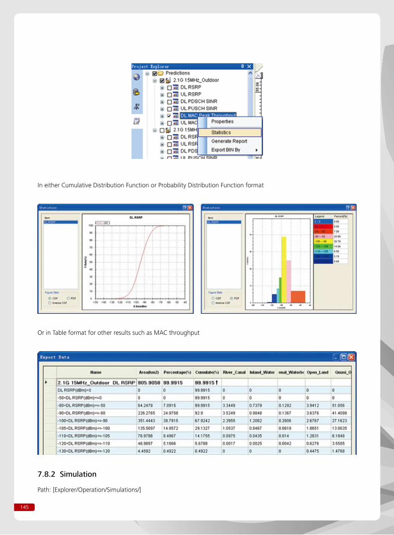
145
In either Cumulative Distribution Function or Probability Distribution Function format
Or in Table format for other results such as MAC throughput
7.8.2 Simulation
Path: [Explorer/Operation/Simulations/]
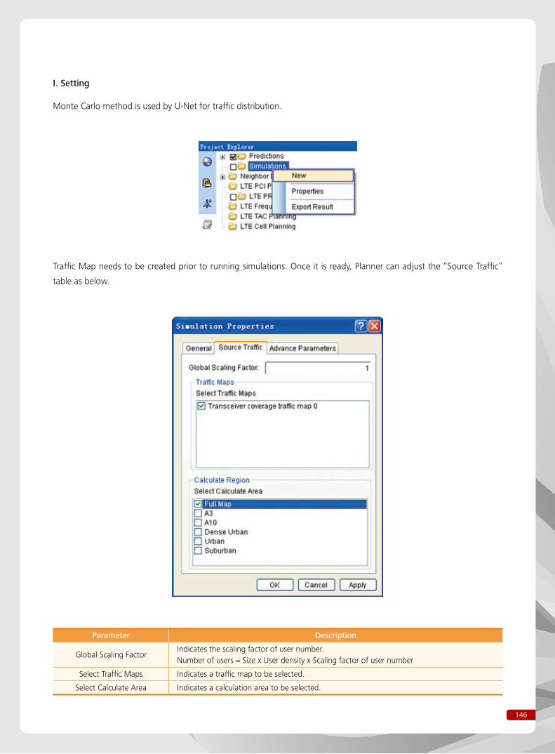
146
Traffic Map needs to be created prior to running simulations. Once it is ready, Planner can adjust the “Source Traffic”
table as below.
Parameter Description
Global Scaling FactorIndicates the scaling factor of user number.Number of users = Size x User density x Scaling factor of user number
Select Traffic Maps Indicates a traffic map to be selected.
Select Calculate Area Indicates a calculation area to be selected.
I. Setting
Monte Carlo method is used by U-Net for traffic distribution.
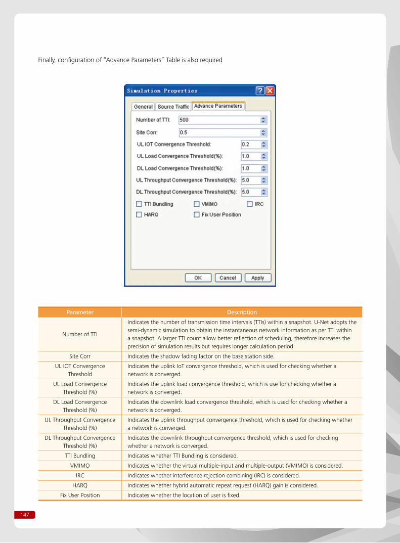
147
Finally, configuration of “Advance Parameters” Table is also required
Parameter Description
Number of TTI
Indicates the number of transmission time intervals (TTIs) within a snapshot. U-Net adopts the semi-dynamic simulation to obtain the instantaneous network information as per TTI within a snapshot. A larger TTI count allow better reflection of scheduling, therefore increases the precision of simulation results but requires longer calculation period.
Site Corr Indicates the shadow fading factor on the base station side.
UL IOT Convergence Threshold
Indicates the uplink IoT convergence threshold, which is used for checking whether a network is converged.
UL Load Convergence Threshold (%)
Indicates the uplink load convergence threshold, which is use for checking whether a network is converged.
DL Load Convergence Threshold (%)
Indicates the downlink load convergence threshold, which is used for checking whether a network is converged.
UL Throughput Convergence Threshold (%)
Indicates the uplink throughput convergence threshold, which is used for checking whether a network is converged.
DL Throughput Convergence Threshold (%)
Indicates the downlink throughput convergence threshold, which is used for checking whether a network is converged.
TTI Bundling Indicates whether TTI Bundling is considered.
VMIMO Indicates whether the virtual multiple-input and multiple-output (VMIMO) is considered.
IRC Indicates whether interference rejection combining (IRC) is considered.
HARQ Indicates whether hybrid automatic repeat request (HARQ) gain is considered.
Fix User Position Indicates whether the location of user is fixed.
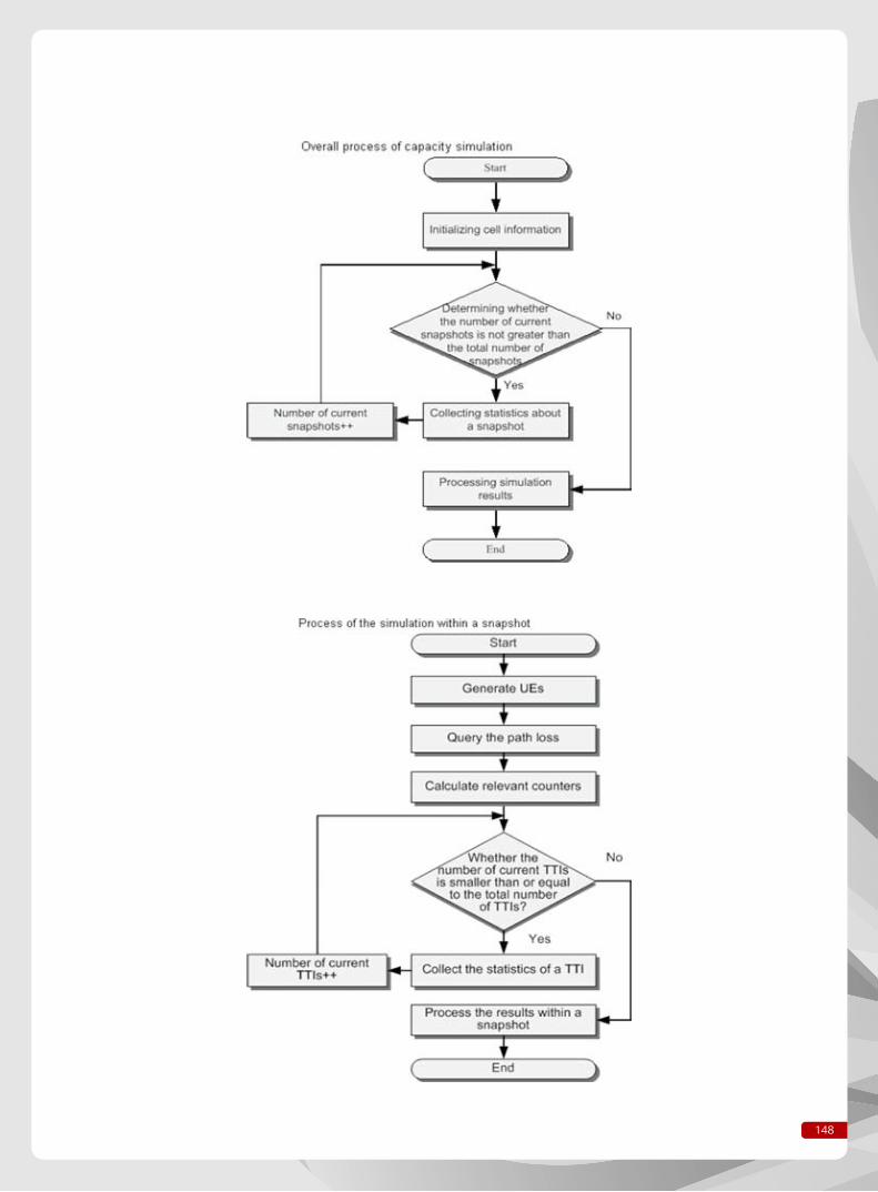
148
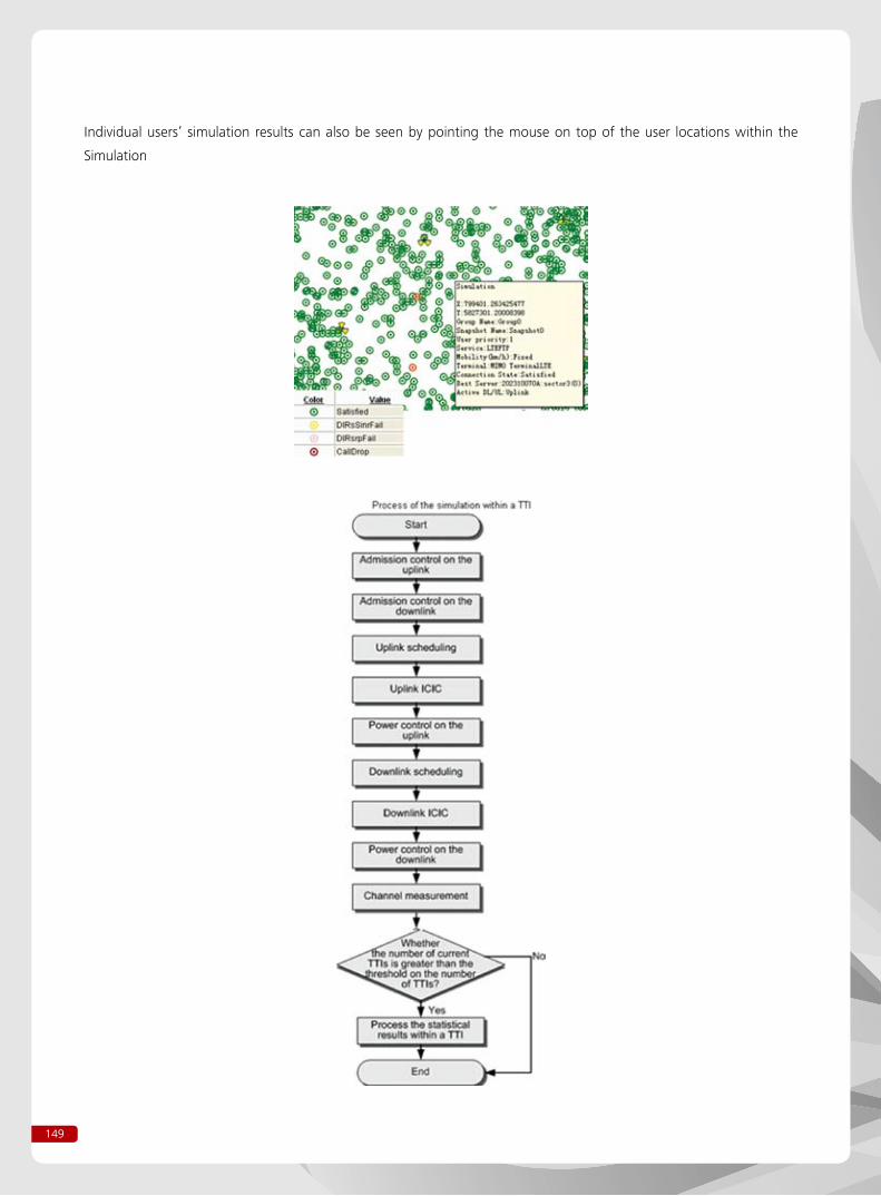
149
Individual users’ simulation results can also be seen by pointing the mouse on top of the user locations within the
Simulation
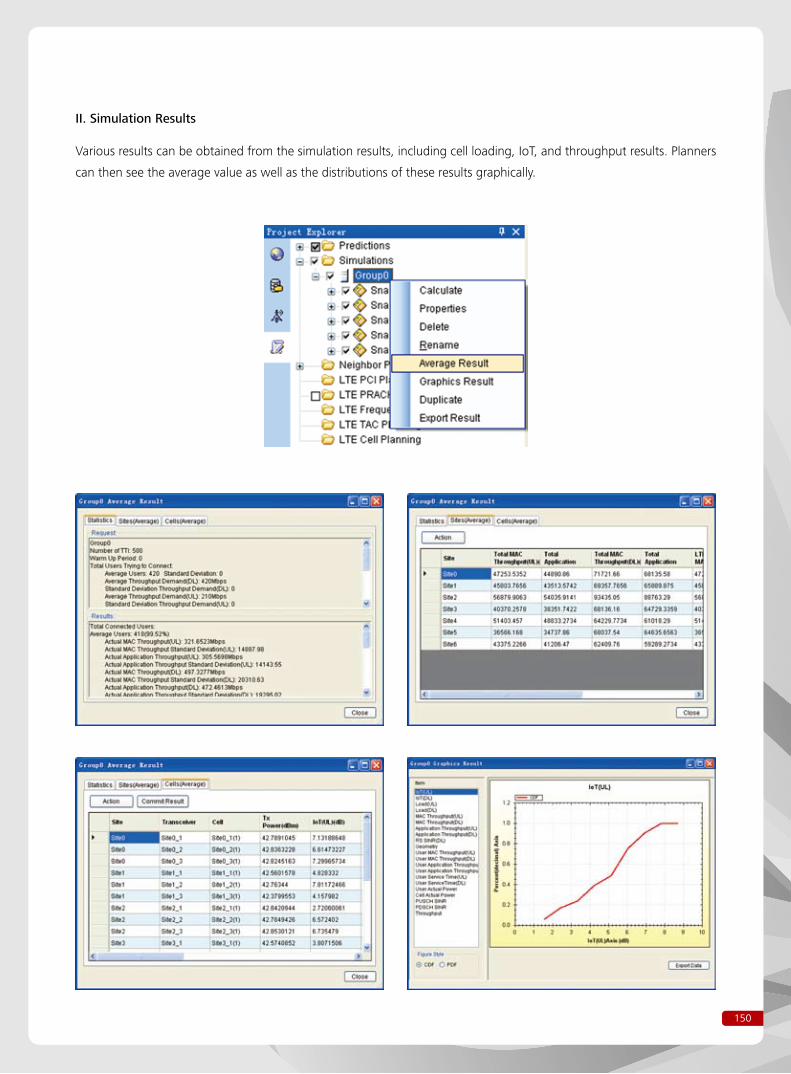
150
II. Simulation Results
Various results can be obtained from the simulation results, including cell loading, IoT, and throughput results. Planners
can then see the average value as well as the distributions of these results graphically.
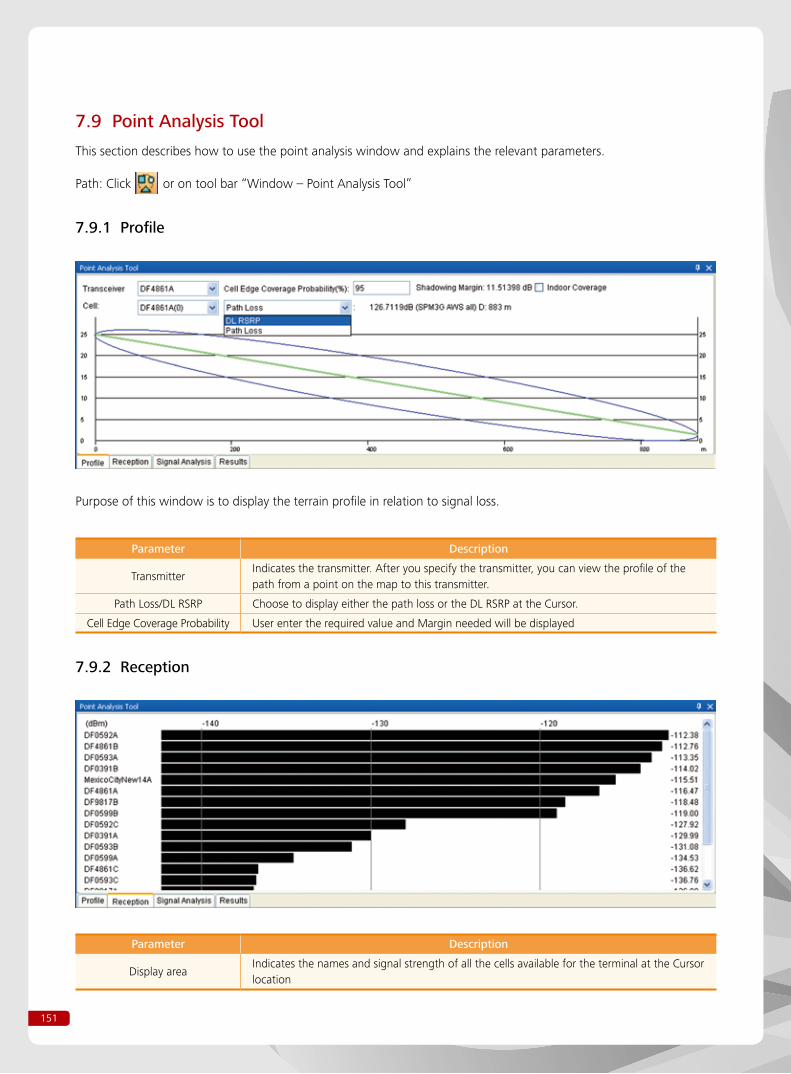
151
7.9 Point Analysis Tool
This section describes how to use the point analysis window and explains the relevant parameters.
Path: Click or on tool bar “Window – Point Analysis Tool”
7.9.1 Profile
Purpose of this window is to display the terrain profile in relation to signal loss.
Parameter Description
TransmitterIndicates the transmitter. After you specify the transmitter, you can view the profile of the path from a point on the map to this transmitter.
Path Loss/DL RSRP Choose to display either the path loss or the DL RSRP at the Cursor.
Cell Edge Coverage Probability User enter the required value and Margin needed will be displayed
Parameter Description
Display areaIndicates the names and signal strength of all the cells available for the terminal at the Cursor location
7.9.2 Reception
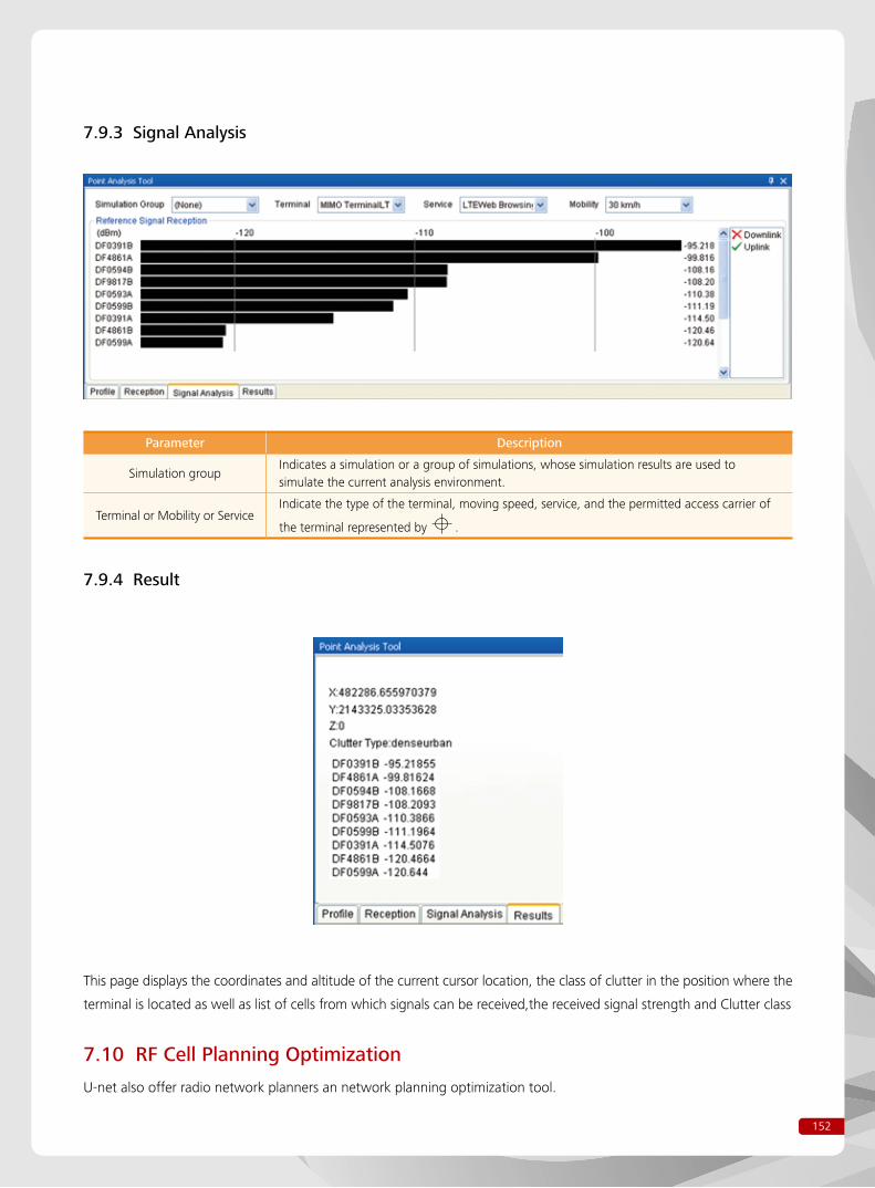
152
7.9.3 Signal Analysis
Parameter Description
Simulation groupIndicates a simulation or a group of simulations, whose simulation results are used to simulate the current analysis environment.
Terminal or Mobility or ServiceIndicate the type of the terminal, moving speed, service, and the permitted access carrier of
the terminal represented by .
7.9.4 Result
This page displays the coordinates and altitude of the current cursor location, the class of clutter in the position where the
terminal is located as well as list of cells from which signals can be received,the received signal strength and Clutter class
7.10 RF Cell Planning Optimization
U-net also offer radio network planners an network planning optimization tool.
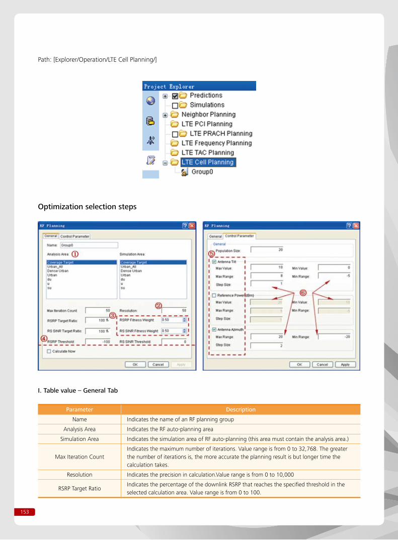
153
Path: [Explorer/Operation/LTE Cell Planning/]
Optimization selection steps
I. Table value – General Tab
Parameter Description
Name Indicates the name of an RF planning group
Analysis Area Indicates the RF auto-planning area
Simulation Area Indicates the simulation area of RF auto-planning (this area must contain the analysis area.)
Max Iteration CountIndicates the maximum number of iterations. Value range is from 0 to 32,768. The greater the number of iterations is, the more accurate the planning result is but longer time the calculation takes.
Resolution Indicates the precision in calculation.Value range is from 0 to 10,000
RSRP Target RatioIndicates the percentage of the downlink RSRP that reaches the specified threshold in the selected calculation area. Value range is from 0 to 100.
154
Parameter Description
RSRP FitnessWeightIndicates the weight of the RSRP performance counter of a cell. Value range is from 0 to 1. RS SINR Fitness Weight + RSRP Fitness Weight = 1
RS SINR Fitness WeightIndicates the weight of the RS SINR performance counter of a cell. Value range is from 0 to 1. RS SINR Fitness Weight + RSRP Fitness Weight = 1
RS SINR Target RatioIndicates the percentage of the downlink RS SINR that reaches the specified threshold in the selected calculation area.
Calculate Now Indicates whether to perform the RF auto-planning immediately
Parameter Description
Population Size
Indicates the size of a population, that is, the total number of individuals in a population. In U-Net, an individual represents the configuration combination of the RF parameters related to all the cells in a calculation area. Individuals of Population Size are calculated in each iteration and the greater the number of individuals, the more accurate the planning result is, but the longer time the calculation takes. Value range is from 10 to 40.
Antenna Tilt Max or Min Value
Indicates the maximum/minimum downtilt angle. Value range is from -90 to 90.
Antenna Tilt Max RangeIndicates the maximum adjustment range of the downtilt angle.The value range is from 0 to 180.
Antenna Tilt Min RangeIndicates the minimum adjustment range of the downtilt angle. The value range is from -180 to 0.
Tilt Step Size Indicates the step length at which the downtilt angle is adjusted. Value range is from 0 to 90.
Reference Power Max or Min (dBm)
Indicates the maximum/minimum transmit power of the reference signal. Value range is from -32,768 to 32,768.
Maximum RangeIndicates the maximum adjustment range of the reference signal. Value range is from 0 to 32,768
Minimum RangeIndicates the minimum adjustment range of the reference signal. Value range is from -32,768 to 0.
Power Step SizeIndicates the step length at which the reference signal is adjusted. Value range is from 0 to 32,768.
Antenna Azimuth Max Range Indicates the maximum adjustment range of the azimuth. Value range is from 0 to 360.
Antenna Azimuth Min Range Indicates the minimum adjustment range of the azimuth. Value range is from -360 to 0.
Antenna Azimuth Step Size Indicates the step length at which the azimuth is adjusted. Value range is from 0 to 360.
II. Control Parameter
7.11 U-Net Planning Case
U-Net is widely applied in global LTE planning projects by RNP engineers. Here is one case presented as reference.
7.11.1 Overview of Planning Area
The clutter information and planning target area of City X are presented as below. The planning area is about 30
square km and shown as the red broken line polygon. Main morphologies include Dense Urban, Urban and Suburban.
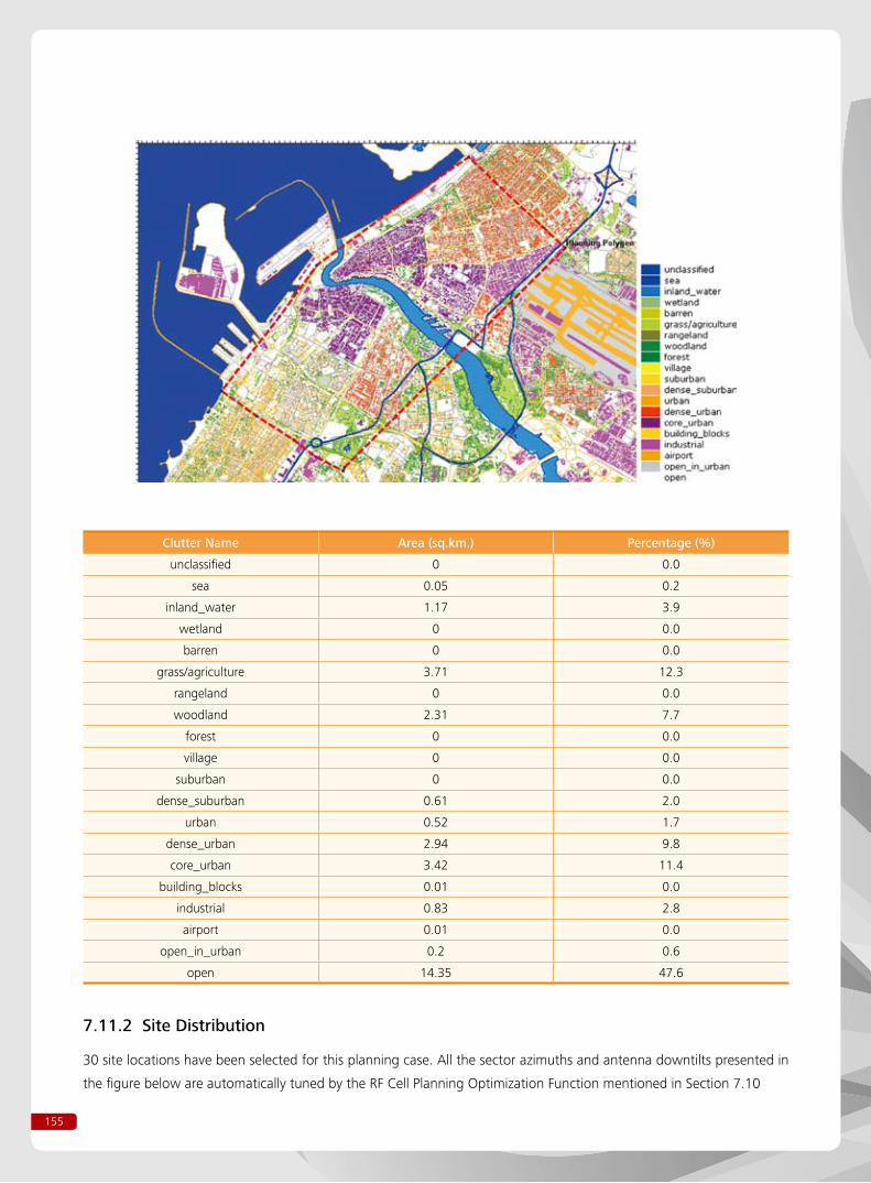
155
7.11.2 Site Distribution
30 site locations have been selected for this planning case. All the sector azimuths and antenna downtilts presented in
the figure below are automatically tuned by the RF Cell Planning Optimization Function mentioned in Section 7.10
Clutter Name Area (sq.km.) Percentage (%)
unclassified 0 0.0
sea 0.05 0.2
inland_water 1.17 3.9
wetland 0 0.0
barren 0 0.0
grass/agriculture 3.71 12.3
rangeland 0 0.0
woodland 2.31 7.7
forest 0 0.0
village 0 0.0
suburban 0 0.0
dense_suburban 0.61 2.0
urban 0.52 1.7
dense_urban 2.94 9.8
core_urban 3.42 11.4
building_blocks 0.01 0.0
industrial 0.83 2.8
airport 0.01 0.0
open_in_urban 0.2 0.6
open 14.35 47.6
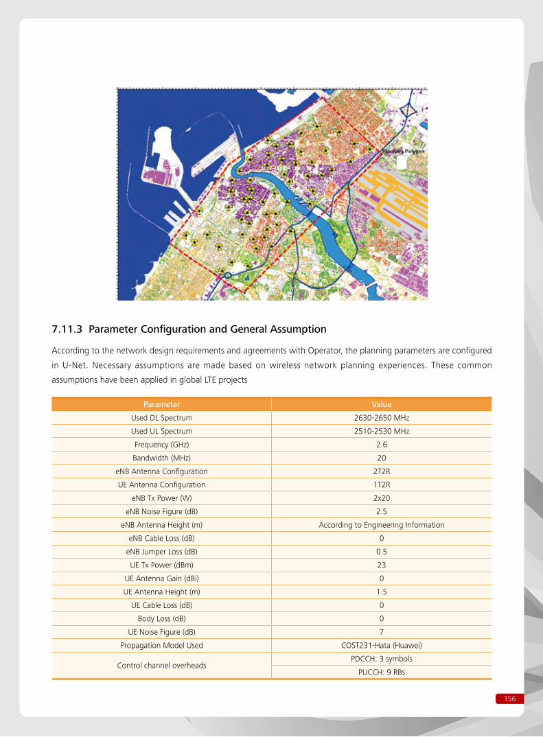
156
7.11.3 Parameter Configuration and General Assumption
According to the network design requirements and agreements with Operator, the planning parameters are configured
in U-Net. Necessary assumptions are made based on wireless network planning experiences. These common
assumptions have been applied in global LTE projects
Parameter Value
Used DL Spectrum 2630-2650 MHz
Used UL Spectrum 2510-2530 MHz
Frequency (GHz) 2.6
Bandwidth (MHz) 20
eNB Antenna Configuration 2T2R
UE Antenna Configuration 1T2R
eNB Tx Power (W) 2x20
eNB Noise Figure (dB) 2.5
eNB Antenna Height (m) According to Engineering Information
eNB Cable Loss (dB) 0
eNB Jumper Loss (dB) 0.5
UE Tx Power (dBm) 23
UE Antenna Gain (dBi) 0
UE Antenna Height (m) 1.5
UE Cable Loss (dB) 0
Body Loss (dB) 0
UE Noise Figure (dB) 7
Propagation Model Used COST231-Hata (Huawei)
Control channel overheadsPDCCH: 3 symbols
PUCCH: 9 RBs
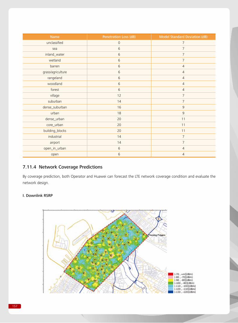
157
Name Penetration Loss (dB) Model Standard Deviation (dB)
unclassified 0 7
sea 6 7
inland_water 6 7
wetland 6 7
barren 6 4
grass/agriculture 6 4
rangeland 6 4
woodland 6 4
forest 6 4
village 12 7
suburban 14 7
dense_suburban 16 9
urban 18 9
dense_urban 20 11
core_urban 20 11
building_blocks 20 11
industrial 14 7
airport 14 7
open_in_urban 6 4
open 6 4
7.11.4 Network Coverage Predictions
By coverage prediction, both Operator and Huawei can forecast the LTE network coverage condition and evaluate the
network design.
I. Downlink RSRP
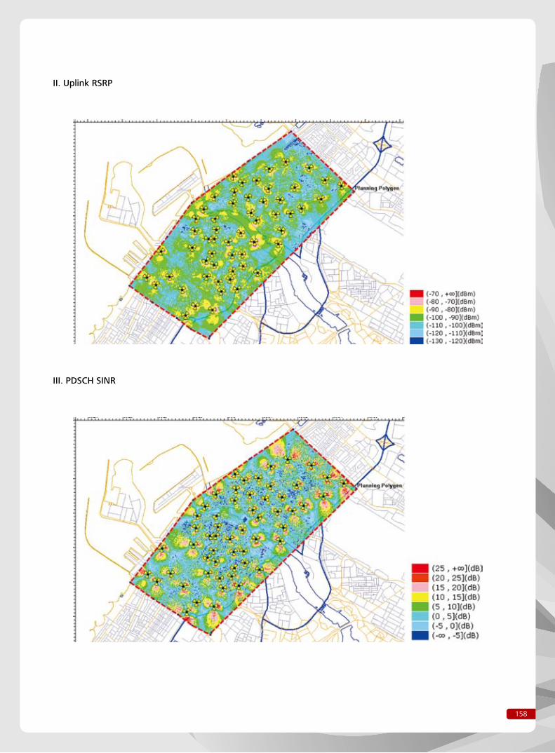
158
II. Uplink RSRP
III. PDSCH SINR
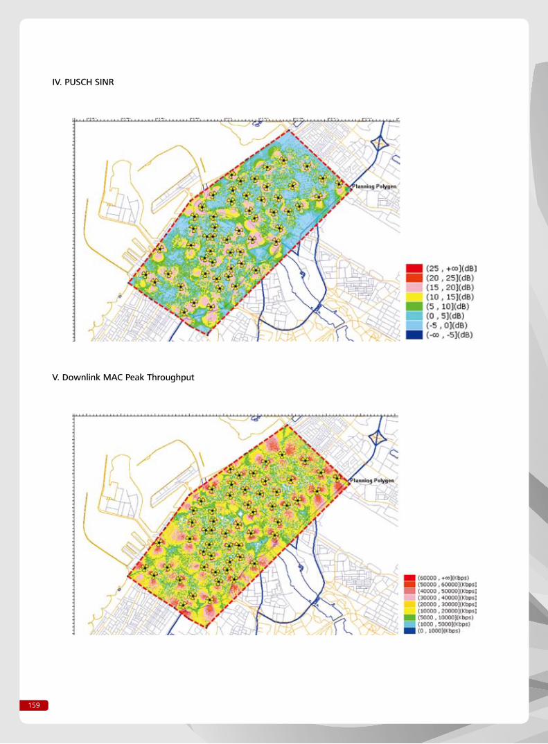
159
IV. PUSCH SINR
V. Downlink MAC Peak Throughput
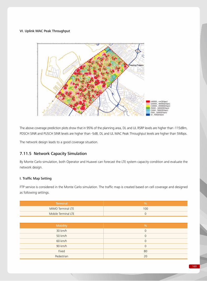
160
Terminal %
MIMO Terminal LTE 100
Mobile Terminal LTE 0
Mobility %
30 km/h 0
50 km/h 0
60 km/h 0
90 km/h 0
Fixed 80
Pedestrian 20
VI. Uplink MAC Peak Throughput
The above coverage prediction plots show that in 95% of the planning area, DL and UL RSRP levels are higher than -115dBm,
PDSCH SINR and PUSCH SINR levels are higher than -5dB, DL and UL MAC Peak Throughput levels are higher than 5Mbps.
The network design leads to a good coverage situation.
7.11.5 Network Capacity Simulation
By Monte Carlo simulation, both Operator and Huawei can forecast the LTE system capacity condition and evaluate the
network design.
I. Traffic Map Setting
FTP service is considered in the Monte Carlo simulation. The traffic map is created based on cell coverage and designed
as following settings.
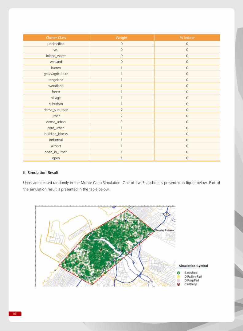
161
II. Simulation Result
Users are created randomly in the Monte Carlo Simulation. One of five Snapshots is presented in figure below. Part of
the simulation result is presented in the table below.
Clutter Class Weight % Indoor
unclassified 0 0
sea 0 0
inland_water 0 0
wetland 0 0
barren 1 0
grass/agriculture 1 0
rangeland 1 0
woodland 1 0
forest 1 0
village 1 0
suburban 1 0
dense_suburban 2 0
urban 2 0
dense_urban 3 0
core_urban 1 0
building_blocks 1 0
industrial 1 0
airport 1 0
open_in_urban 1 0
open 1 0
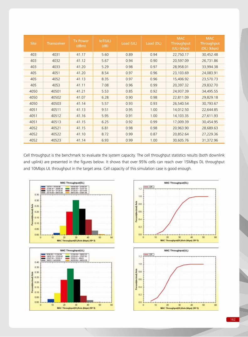
162
Site TransceiverTx Power
(dBm)IoT(UL)
(dB)Load (UL) Load (DL)
MAC Throughput (UL) (kbps)
MAC Throughput (DL) (kbps)
403 4031 41.17 5.60 0.89 0.94 22,750.17 30,452.48
403 4032 41.12 5.67 0.94 0.90 20,597.09 26,731.86
403 4033 41.20 5.29 0.98 0.97 28,958.01 33,994.38
405 4051 41.20 8.54 0.97 0.96 23,103.69 24,083.91
405 4052 41.13 8.35 0.97 0.96 15,406.92 23,570.73
405 4053 41.11 7.08 0.96 0.99 20,397.32 29,832.70
4050 40501 41.21 5.53 0.85 0.92 24,937.39 34,495.55
4050 40502 41.07 6.28 0.90 0.98 22,811.09 29,829.18
4050 40503 41.14 5.57 0.93 0.93 26,540.54 30,793.67
4051 40511 41.13 9.51 0.95 1.00 14,012.50 22,644.85
4051 40512 41.16 5.95 0.91 1.00 14,103.35 27,611.93
4051 40513 41.15 6.25 0.92 0.99 17,009.39 30,454.95
4052 40521 41.15 6.81 0.98 0.98 20,963.90 28,689.63
4052 40522 41.10 8.72 0.99 0.87 20,852.64 27,229.36
4052 40523 41.14 6.93 0.99 1.00 30,605.76 31,372.96
Cell throughput is the benchmark to evaluate the system capacity. The cell throughput statistics results (both downlink
and uplink) are presented in the figures below. It shows that over 95% cells can reach over 15Mbps DL throughput
and 10Mbps UL throughput in the target area. Cell capacity of this simulation case is good enough.
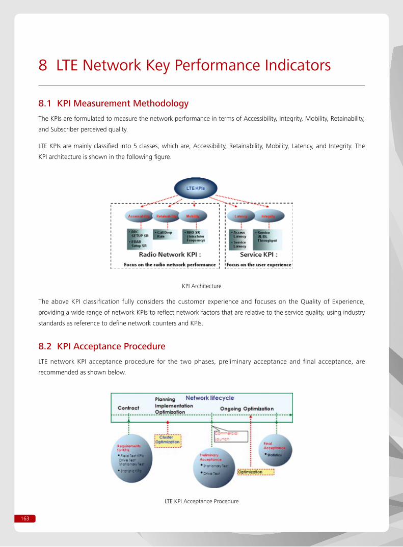
163
8 LTE Network Key Performance Indicators
8.1 KPI Measurement Methodology
The KPIs are formulated to measure the network performance in terms of Accessibility, Integrity, Mobility, Retainability,
and Subscriber perceived quality.
LTE KPIs are mainly classified into 5 classes, which are, Accessibility, Retainability, Mobility, Latency, and Integrity. The
KPI architecture is shown in the following figure.
The above KPI classification fully considers the customer experience and focuses on the Quality of Experience,
providing a wide range of network KPIs to reflect network factors that are relative to the service quality, using industry
standards as reference to define network counters and KPIs.
8.2 KPI Acceptance Procedure
LTE network KPI acceptance procedure for the two phases, preliminary acceptance and final acceptance, are
recommended as shown below.
KPI Architecture
LTE KPI Acceptance Procedure
164
During the phase of preliminary acceptance before commercial launch, KPIs will be derived from the drive test analysis
and stationary measurements, and this analysis and measurement are on the basis of cluster which constitutes a group
of sites (20-40 sites).
Statistics KPIs are not proposed and measured at this stage as the traffic is insufficient, statistics will not eligible
statistical result without enough samples.
After on-going optimization while the traffic keeps increasing after commercial launch, the final acceptance of the
whole network performance on the basis of statistics will be implemented. However, the KPI values of statistics
probably might not be same with those in drive test due to different calculations and considerations.
8.3 Service KPIs and Network KPIs
The Field Test KPIs into two categories: Service KPIs and Network KPIs.
Service KPIs are the KPIs that are not subject to be effected by cluster tuning and optimization activities, mainly
determined by product performance, configuration and parameter setting, e.g. ping delay, throughput, etc. We
recommend that only one cluster (named pilot cluster) is selected for the evaluation and acceptance for the Service
KPIs, no necessary for repeating the measurement in all clusters
Based on the above reasons, the Service KPIs’ test is suggested to be performed by Stationary Test (ST) in the area with
good RF conditions and close to the cell in order to eliminate the affect of poor RF or non-equipment factor and the
test is proposed to be implemented under the condition of one serving cell.
Whereas, for Network KPIs, such as Call setup success rate, Call Drop Rate, Handover Success Rate, which is
determined by the radio network environment, planning and optimization capabilities, should be performed on the
Drive Test (DT) routes in rollout clusters.
8.4 Cluster and Test Route
The following contents present recommendation for Cluster Optimization and the selection of Drive Test Route for this
project.,
(1) Cluster Optimization
Performing optimization/acceptance per Cluster is recommended. Cluster means a group of sites (Normally 20-40
sites) which are geographically neighbor and all the eNodeBs of this test cluster should be integrated and on air,
along with surrounding neighbor cells, but the actual sites number of per cluster should be flexible to allow a faster
rollout and acceptance.
(2) Drive Test Route Selection
For cluster optimization, the planning of the test route shall consider the handover performance, neighboring
relations, coverage, etc. In general the test routes shall be planned according to the following criteria:
(a) All sectors of each site in the cluster should be covered by the drive route, if possible.
(b) Routes shall pass through Key business centers, major roads, shopping centers, tourist attractions and railway stations.
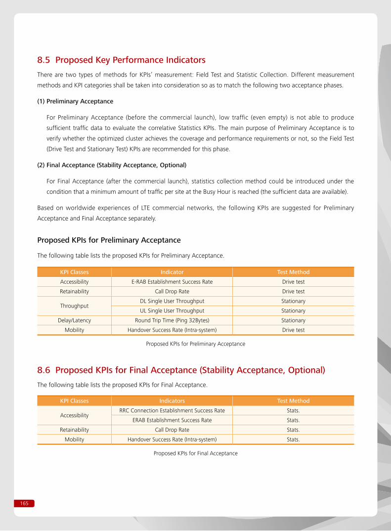
165
8.5 Proposed Key Performance Indicators
There are two types of methods for KPIs’ measurement: Field Test and Statistic Collection. Different measurement
methods and KPI categories shall be taken into consideration so as to match the following two acceptance phases.
(1) Preliminary Acceptance
For Preliminary Acceptance (before the commercial launch), low traffic (even empty) is not able to produce
sufficient traffic data to evaluate the correlative Statistics KPIs. The main purpose of Preliminary Acceptance is to
verify whether the optimized cluster achieves the coverage and performance requirements or not, so the Field Test
(Drive Test and Stationary Test) KPIs are recommended for this phase.
(2) Final Acceptance (Stability Acceptance, Optional)
For Final Acceptance (after the commercial launch), statistics collection method could be introduced under the
condition that a minimum amount of traffic per site at the Busy Hour is reached (the sufficient data are available).
Based on worldwide experiences of LTE commercial networks, the following KPIs are suggested for Preliminary
Acceptance and Final Acceptance separately.
Proposed KPIs for Preliminary Acceptance
The following table lists the proposed KPIs for Preliminary Acceptance.
KPI Classes Indicator Test Method
Accessibility E-RAB Establishment Success Rate Drive test
Retainability Call Drop Rate Drive test
ThroughputDL Single User Throughput Stationary
UL Single User Throughput Stationary
Delay/Latency Round Trip Time (Ping 32Bytes) Stationary
Mobility Handover Success Rate (Intra-system) Drive test
Proposed KPIs for Preliminary Acceptance
KPI Classes Indicators Test Method
AccessibilityRRC Connection Establishment Success Rate Stats.
ERAB Establishment Success Rate Stats.
Retainability Call Drop Rate Stats.
Mobility Handover Success Rate (Intra-system) Stats.
Proposed KPIs for Final Acceptance
8.6 Proposed KPIs for Final Acceptance (Stability Acceptance, Optional)
The following table lists the proposed KPIs for Final Acceptance.
166
9 Network Planning Checklist
9.1 Introduction
By now, radio planning engineers should have a good understanding on the technological background, limitations
and considerations required for the planning of a LTE network. This chapter will go through the required information
step by step from a practical implementation perspective to highlight the approach needed for both radio engineers in
deciding on the strategy required for LTE network planning.
The purpose of the checklist is to ensure all the major aspects are considered either from our intelligence or with
customer input. With all these information on hand, the final network plan created will sure be more customer relevant
and less rework will be required.
9.2 Checklist Items Consideration
Radio planning engineers are highly recommended to review the following checklist items in full and confirm the detail
of all these items BEFORE committing to any network site count to begin to perform any network simulation
9.2.1 Understanding Customer Spectrum Bandwidth Availability
The purpose of detail planning is to determine a solid radio network design for possible deployment so radio engineer
should not be using detail planning as a mean to determine or compare the network capacity offering between 5MHz,
10MHz, 15MHz or 20MHz bandwidth.
However, it is generally true downtown area would require higher bandwidth (15MHz or 20MHz) due to higher traffic
requirement while rural and/or suburban area may only require smaller bandwidth (10MHz). Further issues need
clarifications include
Spectrum availability and timeframe e.g. will customer buy more spectrum in same band, different band. •
Will customer need to perform migration or refarming of 2G/3G technologies first before spectrum is available for LTE •
Any government plan for Spectrum recovery (e.g. swapping customer current spectrum to another band) •
Any spectrum licenses restrictions (e.g. Spectrum only available within 100km from City centre) •
Will the entire network be running on the same frequency spectrum (e.g. City is 2.6G but countryside is 800) •
Too often proposals are based on wrong assumptions on spectrum and the available bandwidth that will be used for
new network deployment which results in a significant cost and work implications.
9.2.2 Actual Frequency Band Allocation for LTE
Similar to spectrum bandwidth availability, radio planners need to know which band is to be given for their network.
The final frequency band granted will have a significant impact on site count and hence overall project cost due to the
propagation and pathloss characteristics of different frequency bands.
The same five questions/issues raised in “Understanding Customer Spectrum Bandwidth Availability” also need to be
167
clarified here if it has not be done so before any detail planning activities are to begin.
It is also worth noting here although the bits/Hz value will not change with different frequency band (i.e. per cell
capacity is bandwidth not frequency band dependent), the final capacity offer by the network will be different due
to the coverage requirement. This is mainly because the final site count is more likely to be determined by coverage
requirement and the capacity offered by the network is the product of site count x capacity per site.
9.2.3 Frequency Band Refarming Requirement for LTE
Some of the most popular questions from customer these days are
How they can perform refarming? •
When is the best time? •
How much spectrum do they need? •
For radio planners, answers to these questions are highly variable and every network will be different due to their
current capacity status, growth forecast, marketing strategies and even management preferences to showcase their
technological leadership or not. As a result, it is recommended until a clear vision is obtained from customer for all 3
questions listed above, no detail network design activities should begin.
In case where LTE is to be introduced after spectrum refarming, the following items will need to be considered carefully
prior to detail network design:
Any co-location with Existing Technology (2G/3G)? •
Guard Band in place already? If not, Guard band spectrum availability? •
Additional passive equipment/path loss introduced due to possible equipment swap out (e.g. antennae change, •
jumper cable, coupler or splitter addition) to enable co-siting with existing technology (CDMA/GSM/UMTS)
Changes in Hardware (e.g. RRU, TMA) which will lead to path loss changes. •
Extra workload requirement due to refarming which may have human resources impact (e.g. require GSM planning). •
Not necessary LTE specific but will be required by 2G/3G e.g. introducing TFR to improve GSM efficiency first.
9.2.4 Location of Customer Coverage Requirement
It is critical to have the proposed LTE site locations correspond to where it can best serve the designated traffic area
and traffic type. In developed markets, high subscriber density and high usage is expected for dense urban and city
area, hence it is normal to have more site count being allocated to dense urban/urban environment.
Currently, there is also a big push in Europe for white spot (rural) wireless DSL coverage in Europe DD spectrum based
on LTE. Therefore, different customers will have different focus on traffic requirement.
In general, high subscriber density area are most likely made up of users with low mobility so the emphasis on site
placement for dense urban is more critical and it is important to be closer to users in high traffic area. On the other
hand, in rural and highway condition, users are likely to be of lower usage and of higher speed so maximizing
coverage through site antenna height or higher terrain is more important.
In summary, radio planning engineers need to have a good understanding of where customer traffic will be in order
to allocate an appropriate distribution of base stations. This allocation can be affected by such factors as indoor
168
penetration margin and slow fading margin in the link budget. If customer focus is just in covering dense urban area, it
will be inappropriate to design a radio network with solid coverage everywhere (suburban/rural alike) where customer
do not appreciate the value or return on their investment.
9.2.5 Highway and Tunnel Coverage Requirement
Most Operators will require good coverage along major highway and major tunnels due to the strategic visibility of
services. In both situations, traffic likely to be high speed but low volume so smaller capacity provisioning is acceptable. In
LTE, this means either smaller bandwidth, small transmit power or even less MIMO complexity as long as coverage is fine.
One major problem for this type of coverage is the feasibility of installation due to for example space and air
conditioning restrictions inside tunnel or location restrictions along major highway so Radio planner also need to
ensure the appropriate type of eNodeB is chosen. In general, it is NOT a good practice to rely on the external eNodeBs
to provide coverage inside the tunnel.
9.2.6 Evaluate Existing Network Condition for InterRAT
Radio planning engineers need to understand the existing customer’s network configuration as well as its footprint.
This is particularly important before designing any network that requires commitment on KPIs later. In any Greenfield
LTE deployment, there will be a need for InterRAT handover either due to coverage hole within the LTE network or on
the fringe of the LTE network to area beyond its coverage.
Hence, understanding the current status of the underlying network from both a coverage and performance perspective
is critical in finalizing the LTE network design and capacity planning. For example,
It is unwise to place an InterRAT border in a heavily congested area. •
Similarly, it is not appropriate to locate an InterRAT border in location where the existing 3G or 2G network is of •
poor coverage.
It is also not recommended to place any InterRAT border along interRNC/BSC or inter PLMN border area. •
Try to locate LTE InterRAT border in area where customer network is offering good throughput to reduce the level •
of future customer complaint.
In order to make these InterRAT boundary decision intelligently, it is reasonable to request traffic loading and
performance information from the customer regarding the existing network both within and on the edge of the
proposed LTE network
9.2.7 Terrain and Clutter Database Availability and Accuracy
It may not appear to be important but the resolution and accuracy of terrain and clutter information will have a BIG
influence on the reliability of the final network design. Clutter resolution comes as 10m, 25m, 50m, 100m and beyond
depending on the price paid as well as the location of the clutter. For instance, downtown area will require higher
resolution while rural town can accept data of a lower resolution nature.
Besides data resolution, it is also important to ensure the clutter data is not shifted from the real structural location.
Another important factor is when the database was made available and when was the latest update made. It is very
worthwhile to valid the clutter information against other sources of information e.g. Google earth (which is normally 3
169
to 6 months late) to ensure critical structures have been included.
9.2.8 Scheduler Selection
Radio design engineer can choose between different data transmission schedulers in the OSS database depending on
the likely radio performance of the network. Normally, PF scheduling is preferred but Max C/I scheduling will give the
best throughput for a network with solid coverage.
9.2.9 Indoor Coverage Requirement
Customer coverage expectation will have a direct impact on link budget considerations for both indoor penetration
requirement and standard deviation. The final requirement of site count will thereby be directly impacted.
Nevertheless, at important indoor locations such as lobbies of major hotels, popular sport stadium, subway stations
and airports, there is always a need of indoor microcell and customer is normally quite willingness to pay for the extra
coverage. On the other hand, customer may have difficulties in accessing certain buildings or shopping malls so these
areas may need to be covered by outdoor eNodeBs which will increase the penetration requirement.
9.2.10 Cell Edge Throughput Requirement
The final requirement of Uplink and Downlink throughput requirement at cell edge has to come from customer and
is directly related to their pricing as well as branding. Sometimes, the edge throughput requirement is also a result of
special government legislation on Operator e.g. white spot coverage in European countries like Germany as well as
rural coverage in US, Canada and Australia.
9.2.11 Call Model and SmartPhone Penetration Growth Considerations
The arrival of Smartphone has introduced a whole new trend in data applications and hence resource usage condition.
There is now a much bigger data requirement especially in short and bursting traffic. As a result, some networks are
seeing single smart-phone user consuming up to 14 times network resources normally consumed by traditional non
smart phone user.
Depending on the network morphologies weighting, final site count will also be affected as it would be unwise to
assume high data traffic usage uniformly across the entire network. It is likely high data usage traffic be concentrated
around dense urban and urban area while Rural and Highway area will consist of lower than average data user. By
assigning appropriate data user model inside U-net, different usage behavior should be simulated accordingly.
Other important questions to be considered before finalizing the network plan are
How much spare capacity the network has to tackle the growth and change in subscriber’s usage without adding •
extra equipment?
How well data hot spots (e.g. big shopping mall, major pedestrian walkways, major stadium and other high profile •
locations) are covered? Do they have dedicated cell coverage?
How much penetration margin is provided for indoor coverage? Indoor user will be a major factor for interference •
generation to other users due to the higher power requirement.
Any major driver for surprise usage increase in the near future? (e.g. Government legislation to improve rural/ •
170
suburban usage, home DSL replacement package, shutting down of existing data network and migrating users to
new LTE networks)
9.2.12 Base Station Antenna and Other Co-siting Equipment Selection
New LTE network is likely to be overlaying with customer’s existing radio networks. Hence, antenna selection would be
a critical factor in the new LTE radio network design. Frequency band of the new LTE network will also be a critical factor
in antenna selection. If SingleRAN solution is already in place and new LTE network is built on frequency band covered by
existing antennae, no additional loss will be incurred. However, this may come at the expense of limitation in tilting flexibility.
On the other hand, if the LTE network is to be overlay on other vendor’s network within the same frequency band,
addition loss (e.g. combiners, splitters and jumper cables) needs to be included in the prediction design to ensure all
the extra combining loss are included due to equipment co-siting.
While use of separate and/or new antenna may incur additional project cost, radio planners need to evaluate the
benefit of having this tilting and orientation flexibility carefully on a site by site basis. Existing radio networks are also
likely to have additional downtilt for coverage control purposes so independent tilt for Greenfield LTE network may
help to reduce the final site count required.
New multiband antennae now offered by Huawei Agisson can provide independent electrical tilt for different band
which may be useful for some situations. However, certain network requirements may demand new antennae
altogether due to different network coverage requirement.
Finally, installation of new antennae in certain locations may not be possible due to local authority restriction, for
example: inside shared antenna system in major shopping malls, tunnels and sporting stadium. Hence, radio engineers
need to ensure project team or customer can provide appropriate installation feasibility for such locations. In general,
engineers should not rely on tunnel coverage to be provided by radio signals coming from the base station located
outside the tunnel premises.
9.2.13 Interference Protection and Isolation Requirement
Similar to any radio network, standard isolation would be required if equipment from different vendors are to be
combined. Please refer to previous discussion in Chapter 5 for guard band, filtering as well as vertical/horizontal
separation information.
In addition, indoor DAS (distributed antenna system) may contribute to interference problem particularly on the
uplink due to PIM related inter-modulation, over drive of input RF power as well as impedance mismatch between
components.
Wideband repeaters operating in the same or even adjacent band to the LTE networks may generate unwelcomed
interference. Due the close vicinity to traditional microwave frequencies, LTE networks at 2.3G to 2.6G may also be
subjected to interference either from standard microwave, satellite transmission or MMDS/LMDS networks. Conversely,
700/800MHz digital dividend spectrum could be subjected to interference signals coming from big television
broadcasting towers. These two factors could lead to extra guard band and worst case full retune requirement for
protection purposes.
171
At certain cell site sectors, antenna orientation and tilt may need to be adjusted to avoid interference from external
sources and existing customer network configuration may give hints in this direction.
Although external interference sometimes could be unavoidable due to various reasons, ideally, radio engineers should
choose a spectrum that is relatively clean in both the uplink and downlink for new LTE systems deployment.
Finally, interference increase due to traffic loading is always an important consideration especially when subscriber
number increases. Careful planning of location update border and coverage control remains two of the most important
techniques in resolving this problem.
9.2.14 Radio Related Equipment Selection
With the introduction of new Remote radio head technology, it is important the benefit of applying such products
is reflected in our design proposal and link budget estimation. For instance, there is a 2.5dB reduction in cable loss
in using DBS RRU (0.5dB) vs Macro RFU (3dB). Radio engineers also need to understand the current configuration
of customer sites so the realistic cable and/or combiner loss are reflected in their coverage design. Normally, a cable
length of 30m is assumed but this definitely needs to be reviewed during the design stage on a site by site basis based
on customer information (e.g. site drawing)
9.2.15 Network and Spectrum Evolution Consideration
Different Operators may have different network evolution considerations. For instance, most FDD based Operators
will likely to be focusing on existing spectrum (850/900/1800MHz) refarming while WiMAX Operators will have major
concern on co-existence between WiMAX and LTE TDD.
All these considerations will affect the selection of network components involved (e.g. filter bandwidth, RRU power
and guard band/spectrum requirement). Depending on the chosen direction, the total path loss will also be different
so radio engineers need to discuss with customer in detail on their plan and preference to ensure the discussion results
are reflected in the detail network design plan.
9.2.16 MIMO and Beam Forming Implementation
The number of antenna deployed per cell will have an immediate impact on the coverage and capacity offered by
diversity based technology like LTE. As a major application for LTE TDD, beam forming is very similar to the diversity
transmission, the main difference being that in beam forming one typically considers a physical antenna beam being
constructed towards the UE. So for best result, beam forming requires closely spaced antennae and this is unlike
the MIMO diversity schemes which require at least a few wavelength antenna spacing. However, due to installation
limitation, beams will be at least a few wavelength apart but the arrival of higher transmit/receive order antenna may
well change this situation in the future.
However, radio engineers need to remember the addition of new antennae may incur extra CAPEX and OPEX cost on
the operator due to extra mounting pole requirement so prior customer discussion is recommended.
9.2.17 Cyclic Prefix Planning
172
Radio engineer should also discuss with customer to ensure any sites needing extended coverage are addressed by
using the Long CP configuration as discussed in Chapter 3 and 6.
9.2.18 Understanding of Current Transmission Backhaul Network Capability
Radio planners should regularly report and remind core and transmission network designers about the LTE access
network transmission capacity requirement based on customer edge throughput and traffic requirement. An
appropriate buffer needs to be provisioned by the transmission planners as there will be extra loading due to S1/X2
interfaces as described in Chapter 6. Result of backhaul congestion will be slower user throughput, possible drop call
and QoS/QoE degradation.
Although the expansion of backhaul capacity will normally occur in conjunction with LTE access network rollout, it is
still essential to ensure no commitment of radio access throughput beyond backhaul latency, capability and capacity is
made. Transmission expansion based on microwave could be lengthy from a time perspective due to various technical
and spectrum regulations so radio planners should report their requirement as soon as possible.
9.2.19 UE Distribution and Channel Model : Pedestrian vs High Mobility
The impact of user distribution (pedestrian oriented vs high mobility focus) needs to be reflected in the channel model
chosen for link budget estimation. On the other hand, appropriate proportioning between mobile and pedestrian users
can also be configured in U-Net Simulations using the correct channel mode under each of the Environment entries.
If the target network is a dense metropolis like Hong Kong, Shanghai or Singapore, using the wrong incorrect (higher
mobility) channel models will have a higher demand on capacity and throughput estimation. On the other hand, for more
mobility oriented cities in Western Europe, North America and Australia/New Zealand, using a more pedestrian oriented
channel model will most likely result in an under-estimation of equipment requirement. This is because power control
works much more efficiently in low mobility environment and its gain diminishes as the speed of mobility increases.
Hence, radio engineers should observe the local condition and make appropriate adjustment in their radio plan.
9.2.20 TDD Specific Uplink and Downlink Configuration
Due to the spectrum sharing and time division nature of TDD, there are seven Downlink vs Uplink assignment ration
as well as nine Uplink/Downlink Pilot Time Slot vs Guard Band configuration available for radio planner’s selection. The
different combination will have an impact on both the coverage and capacity availability especially when there is an
extended range requirement.
Radio engineers are recommended to determine the traffic ratio between downlink and uplink from the customer’s
current network to assist in the selection of appropriate slot assignment ratio. Requirement of extended cell can also
be determined via customer discussion and current network coverage review to minimize provisioning of guard band
in LTE TDD network.
9.2.21 Power Boosting Configuration
Similar to most wireless systems, the perception of customer coverage is likely to be dictated by the “coverage” shown
by UEs (e.g. number of signal bars). Hence, at initial LTE network launch when loading is low, a higher power boosting

173
factor will help to improve coverage perception and reduce cell site count as RSRP is always a major requirement from
customer.
However, once network traffic grows steadily, there will be a need to scale back power boosting as
Power Boosting consumes extra RE that could have been used for traffic •
The higher the MIMO order, the more RE will be consumed •
More new sites are likely to be added to enhance coverage as well as capacity so Power boosting will indeed have •
a negative impact on coverage control in this situation.
174
10 Appendix: RF Antenna Systems
10.1 Overview
Antenna is a device which converts an electric wave guided by a conductor into a free-space, unguided
electromagnetic wave, and vice versa. Electrical energy is fed to the antenna via a transmission line, a conductor which
passes electrical energy from one point to another. A matching device is usually required to ease the abrupt transition
between the guided and the free wave. The wave guided by the line is radiated into space by the antenna.
10.2 Antenna Classification
There are dozens of antenna types and variations of each. The type of antenna selected for use depends on the
propagation characteristics required.
10.2.1 Frequency
Antennas can be classified as single-band antennas (narrow-band antennas), wide-band antennas, dual-band
antennas, triple-band antennas, etc
10.2.2 Directivity
Antennas can be omnidirectional, sector or directive. Omni-directional antennas radiate roughly the same pattern all
around the antenna in a complete 360° pattern. The most popular types of omnidirectional antennas are the dipole
and the ground plane. Sectorial antennas radiate primarily in a specific area. The beam can be as wide as 180 degrees,
or as narrow as 60 degrees. Directional or directive antennas are antennas in which the beamwidth is much narrower
than in sector antennas. They have the highest gain and therefore used for long distance coverage. Types of directive
antennas are the Yagi, the biquad, the horn, the helicoidal, the patch antenna, the parabolic dish, and many others.
10.3 Main Specifications of Antenna
The technical specifications of antenna include:
Work band •
Gain •
Polarization mod •
Beam width •
Preset down tilt •
Down tilt mode •
Adjustable range of down tilt •
Front-to-rear ratio •
Side lobe suppression ratio •
Zero point filling •
Echo loss •

175
Power capacity •
Impedance •
Third order intermodulation •
The mechanical specifications of antenna include:
Dimensions •
Weight •
Number Input ports •
Port connector type (e.g. N or DIN) •
Wind load •
10.3.1 Work Band
It is the work band of LTE system. Huawei Agisson is offering antenna product of the following frequency band:
806-960MHz (FDD 850MHz, 900MHz) •
1710-2170MHz (FDD 1800MHz, 2100MHz, AWS and TDD Band 33-37, Band 39) •
2300-2700MHz (TDD Band 38/40 and FDD 2.6G) •
824-960/1710-2180MHz (Dual Band) •
2300-2700/2300-2700MHz (for 4T4R MIMO) •
The only major band not covered by Huawei Agisson is 700MHz band used mainly for US LTE networks.
10.3.2 Antenna Gain
The antenna is a passive device. It can neither strengthen the signal nor transmit signal by itself. It concentrates the
power to a direction by changing the combination of oscillators and changing the feeder mode. Gain is a key index for
antenna, standing for the capability of concentrating the power to a direction. There are usually two units for antenna
gain: dBi and dBd. The relationship between the two units is as the following equation:
0 dBd = 2.15 dBi
dBi: the capability of concentrating power by actual directional antenna (including omnidirectional) compared with •
the isotropic antenna. The i in dBi means isotropic.
dBd: the capability of concentrating power by actual directional antenna (including omnidirectional) compared with •
half-wave dipole antenna. The d in dBd means dipole.
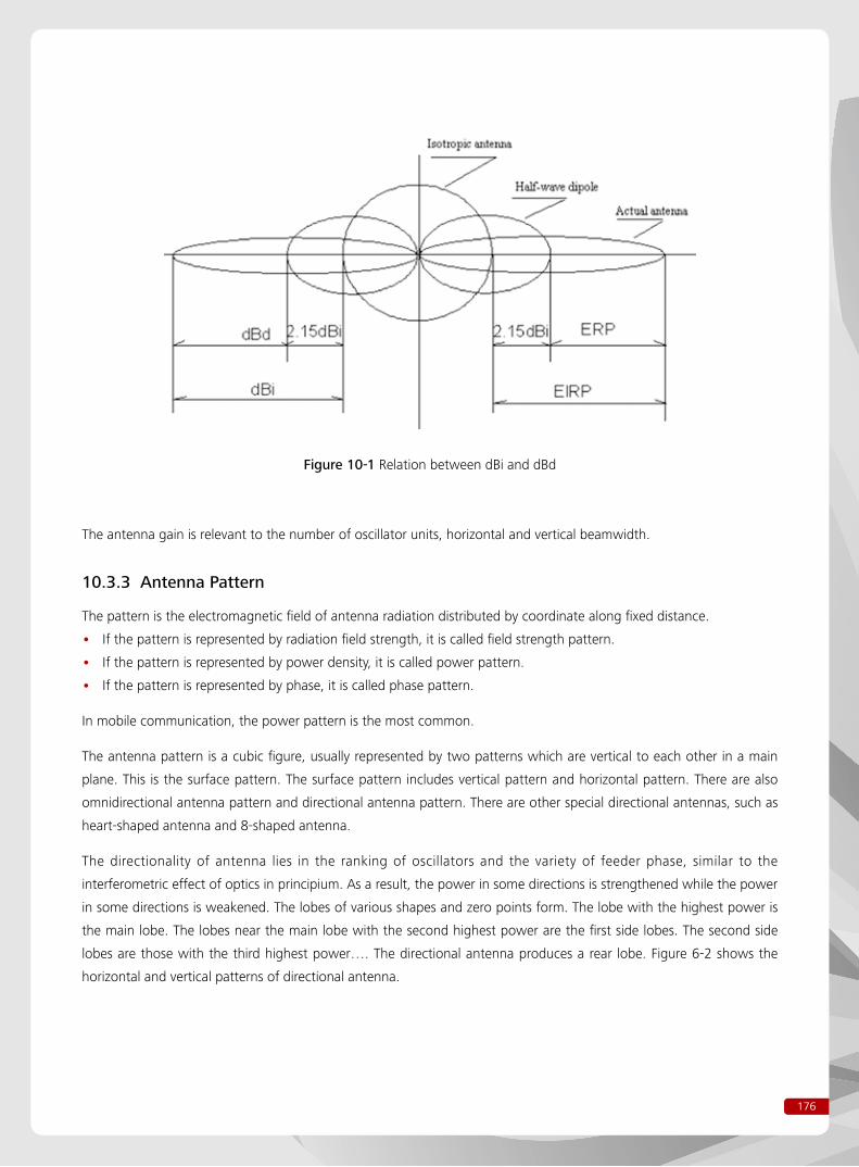
176
Figure 10-1 Relation between dBi and dBd
The antenna gain is relevant to the number of oscillator units, horizontal and vertical beamwidth.
10.3.3 Antenna Pattern
The pattern is the electromagnetic field of antenna radiation distributed by coordinate along fixed distance.
If the pattern is represented by radiation field strength, it is called field strength pattern. •
If the pattern is represented by power density, it is called power pattern. •
If the pattern is represented by phase, it is called phase pattern. •
In mobile communication, the power pattern is the most common.
The antenna pattern is a cubic figure, usually represented by two patterns which are vertical to each other in a main
plane. This is the surface pattern. The surface pattern includes vertical pattern and horizontal pattern. There are also
omnidirectional antenna pattern and directional antenna pattern. There are other special directional antennas, such as
heart-shaped antenna and 8-shaped antenna.
The directionality of antenna lies in the ranking of oscillators and the variety of feeder phase, similar to the
interferometric effect of optics in principium. As a result, the power in some directions is strengthened while the power
in some directions is weakened. The lobes of various shapes and zero points form. The lobe with the highest power is
the main lobe. The lobes near the main lobe with the second highest power are the first side lobes. The second side
lobes are those with the third highest power…. The directional antenna produces a rear lobe. Figure 6-2 shows the
horizontal and vertical patterns of directional antenna.
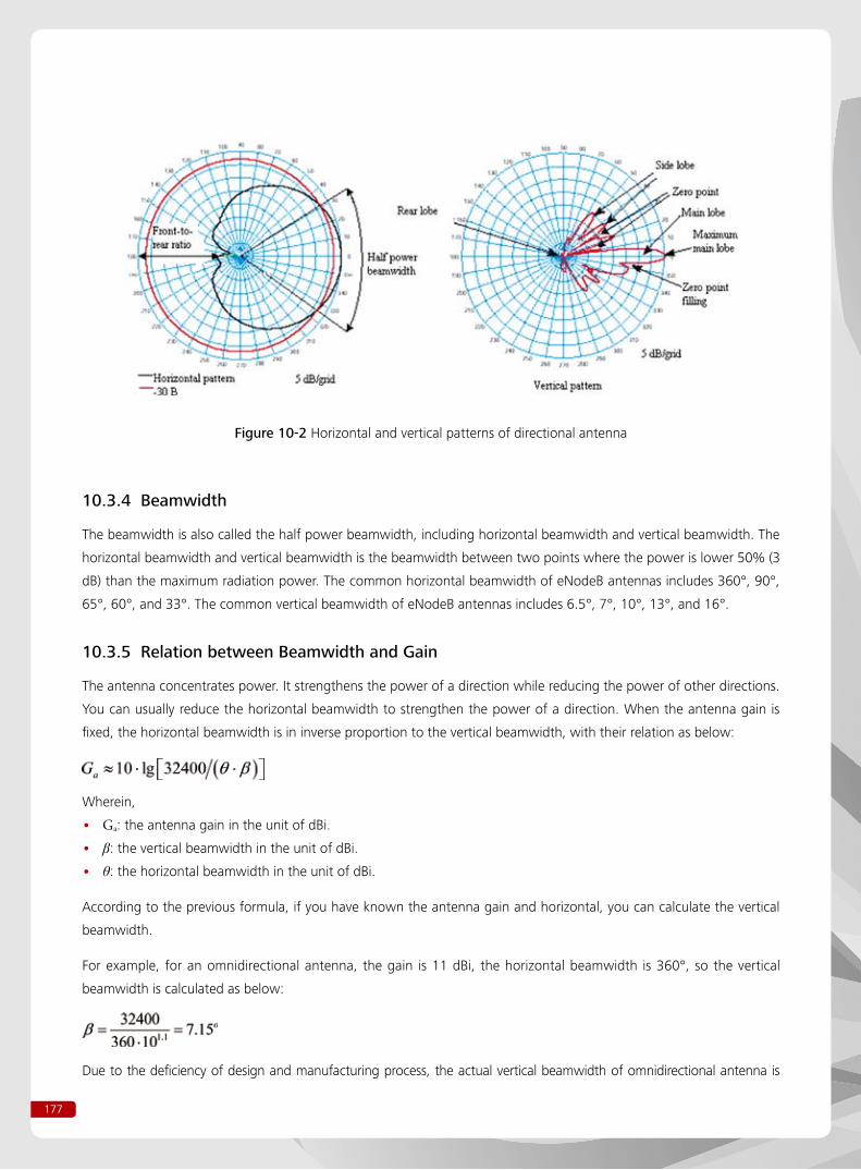
177
Figure 10-2 Horizontal and vertical patterns of directional antenna
10.3.4 Beamwidth
The beamwidth is also called the half power beamwidth, including horizontal beamwidth and vertical beamwidth. The
horizontal beamwidth and vertical beamwidth is the beamwidth between two points where the power is lower 50% (3
dB) than the maximum radiation power. The common horizontal beamwidth of eNodeB antennas includes 360°, 90°,
65°, 60°, and 33°. The common vertical beamwidth of eNodeB antennas includes 6.5°, 7°, 10°, 13°, and 16°.
10.3.5 Relation between Beamwidth and Gain
The antenna concentrates power. It strengthens the power of a direction while reducing the power of other directions.
You can usually reduce the horizontal beamwidth to strengthen the power of a direction. When the antenna gain is
fixed, the horizontal beamwidth is in inverse proportion to the vertical beamwidth, with their relation as below:
Wherein,
G • a: the antenna gain in the unit of dBi.
β • : the vertical beamwidth in the unit of dBi.
θ • : the horizontal beamwidth in the unit of dBi.
According to the previous formula, if you have known the antenna gain and horizontal, you can calculate the vertical
beamwidth.
For example, for an omnidirectional antenna, the gain is 11 dBi, the horizontal beamwidth is 360°, so the vertical
beamwidth is calculated as below:
Due to the deficiency of design and manufacturing process, the actual vertical beamwidth of omnidirectional antenna is
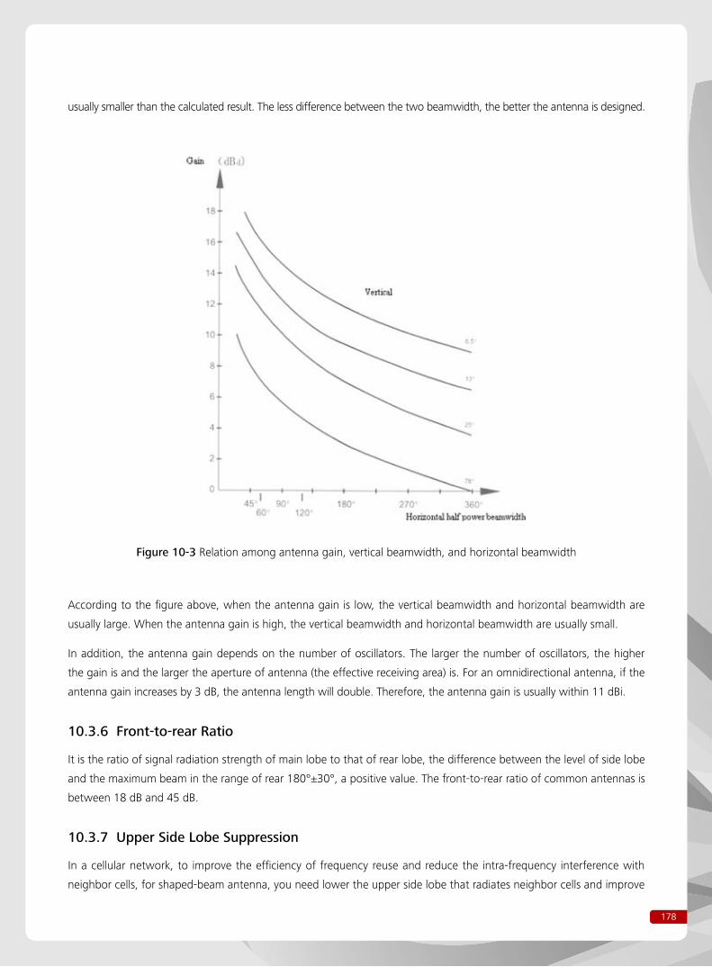
178
usually smaller than the calculated result. The less difference between the two beamwidth, the better the antenna is designed.
Figure 10-3 Relation among antenna gain, vertical beamwidth, and horizontal beamwidth
According to the figure above, when the antenna gain is low, the vertical beamwidth and horizontal beamwidth are
usually large. When the antenna gain is high, the vertical beamwidth and horizontal beamwidth are usually small.
In addition, the antenna gain depends on the number of oscillators. The larger the number of oscillators, the higher
the gain is and the larger the aperture of antenna (the effective receiving area) is. For an omnidirectional antenna, if the
antenna gain increases by 3 dB, the antenna length will double. Therefore, the antenna gain is usually within 11 dBi.
10.3.6 Front-to-rear Ratio
It is the ratio of signal radiation strength of main lobe to that of rear lobe, the difference between the level of side lobe
and the maximum beam in the range of rear 180°±30°, a positive value. The front-to-rear ratio of common antennas is
between 18 dB and 45 dB.
10.3.7 Upper Side Lobe Suppression
In a cellular network, to improve the efficiency of frequency reuse and reduce the intra-frequency interference with
neighbor cells, for shaped-beam antenna, you need lower the upper side lobe that radiates neighbor cells and improve
179
the D/U ratio (the ratio of strength of useful signal to that of interference signal). The level of the first upper side lobe
compared with main lobe shall be smaller than –18 dB. This is invalid to the antennas of macro cell eNodeB.
10.3.8 Polarization Mode
The polarization is a radiation feature for indicating the vector special direction of field strength of electromagnetic
wave. If unspecified, the spatial direction of electric field vector usually serves as the polarization direction of
electromagnetic wave. The spatial direction of electric field vector is the direction of maximum radiation by antenna.
The electromagnetic wave of which the spatial direction of electric filed vector keeps fixed any time is the linear
polarization wave. With the ground as a reference, the polarization of which the direction of electric field vector is
parallel to ground is the horizontal polarization wave and polarization of which the direction of electric field vector is
vertical to ground is the horizontal polarization wave.
The spatial direction of electric field vector is not always fixed.
If the endpoint trace of electric field vector forms a circle, the polarization wave is circular polarization wave. •
If the endpoint trace of electric field vector forms an ellipse, the polarization wave is elliptical polarization wave. •
The elliptical polarization wave and circular polarization wave have polarization direction.
The electromagnetic wave of different bands caters for different polarization modes for propagation. The mobile
communication systems usually choose vertical polarization while the broadcasting systems usually choose horizontal
polarization. The elliptical polarization usually applies for satellite communication.
The polarization modes of antennas include the polarization and dual polarization, and they are all linear polarization.
The dual polarization antenna reduces the impact from multi-path attenuation and improves the quality of signals
received by the eNodeB by using polarization diversity. The dual polarization antenna in LTE networks usually use ±45°
cross polarization mode.
10.3.9 Down Tilt
The down tilt of antenna is an important means that you can enhance the signal level of serving cell and reduce the
interference with other cells. The common down tilt modes include mechanical down tilt, preset electrical down tilt,
and adjustable electrical down tilt (RET antenna) as below:
Mechanical down tilt: you adjust the mechanical down tilt by lowering the support. •
Electrical down tilt: you adjust the electrical down tilt by adjusting the phase of oscillators. After the preset •
electrical down tilt is sold out of the factory, the down tilt cannot be adjusted. The adjustable electrical down tilt is
adjustable.
You can adjust the mechanical down tilt and electrical down tilt simultaneously.
10.3.10 VSWR (Voltage Standing Wave Ratio)
In mobile communication systems, the VSWR of antenna is 1.5:1 at most. Assume that:
Z • A: input impedance of antenna
Z • 0: nominal characteristic impedance

180
So the reflection coefficient is calculated as below:
You can also represent the matching character of port with echo loss as below:
If the VSWR is 1.5:1, the RL is 13.98 dB.
When the input impedance of antenna is not equal to characteristic impedance, the reflected and incident waves form
standing wave after overlapping on the feeder. The ratio of the maximum adjacent voltage of standing wave to the
minimum adjacent voltage of standing wave is the voltage standing wave ratio (VSWR). If the VSWR is over large, the
communication distance will be shortened and the reflected power will return the transmitter. As a result, the power
amplifier may be burnt and the communication system will work abnormally.
10.3.11 Port Isolation
For multi-port antennas, such as dual polarization antenna and dual band dual polarization antenna, the isolation must
exceed 30 dB when the Rx port is the TX port.
10.3.12 Power Capacity
It is the average power capacity. The antenna comprises of coupling parts, such as matching, balancing, and phase
shift, so it can bear a limited power. If the power of a carrier is 20 W and a port of the antenna can support four
carriers at most, the maximum input power of antenna is 80 W. therefore, the power capacity per port shall exceed
150 W (in a 65°C ambient temperature).
10.3.13 Input Port of Antenna
To improve the reliability of passive intermodulation and RF connection, the input port of antenna is 7/16 DIN-Female.
Before the antenna is used, there shall be a protective cap over the port to avoid generating oxide or absorbing
impurity.
10.3.14 Passive Intermodulation (PIM)
The passive intermodulation is caused by non-linearity of the part when the passive parts like connectors, feeders,
antennas, and filters work under high power of multi-carrier. The passive parts are usually considered linear but they
may have non-linearity to some degree under high power due to the following factors:
The contact between different metals •
The contact between the same metal with rough surface •
181
Loose connection •
Rusty or water filled connection •
Magnetic objects •
The intermodulation product interferes with communication systems, and especially the intermodulation products in
the receiver band have severe impact on the receiving performance of system. As a result, there are strict requirements
on the intermodulation feature of passive parts like connectors, cable, and antennas as below:
Passive intermodulation index of connects: ≤ –150 dBc •
Passive intermodulation index of cable: ≤ –170 dBc •
Passive intermodulation index of antenna: ≤ –150 dBc •
10.3.15 Dimensions and Weight of Antenna
To facilitate storage, transport, installation, and safety, the antenna is required to have a size as small as possible and a
weight as light as possible when all the electrical specifications are met.
The operators have more and more strict requirements on the dimensions, weight, and outlook of antenna, so you
must focus on both the technical and non-technical specifications upon antenna selection. In urban areas, the antenna
of eNodeB shall be light, small, and beautiful. In suburban and rural areas, there is no such restriction.
10.3.16 Wind Load
The antennas are usually installed on high buildings or towers. In the littoral areas, the wind is strong with high speed,
so the antennas are required to work normally under a wind speed of 36 m/s and to keep complete under a wind
speed of 55 m/s.
The antenna can usually resist strong wind. In some windy areas, the antennas are damaged due to unstable tower
and pole, so you shall choose the antennas with small surface area.
10.3.17 Work Temperature and Humidity
The antenna of eNodeB shall work in a temperature of –40°C to +65°C and a humidity of 0 to 100%.
10.3.18 Lightning Protection
A direct DC connection of each RF input ports of antenna to the ground is required.
10.3.19 Three-proof Capability
The antenna of eNodeB must capable of damp-proof, salt mist-proof, and leaf mold-proof. For an omnidirectional
antenna, it can also be installed bottom up and meet the three-proof capacity.
10.3.20 Camouflaged Antenna Scheme for Sites
A camouflaged antenna is beautiful, hidden, and according with technical requirements. The camouflaged antenna
aims to keep consistent with the environment and to avoid being noticed so that the mobile communication project
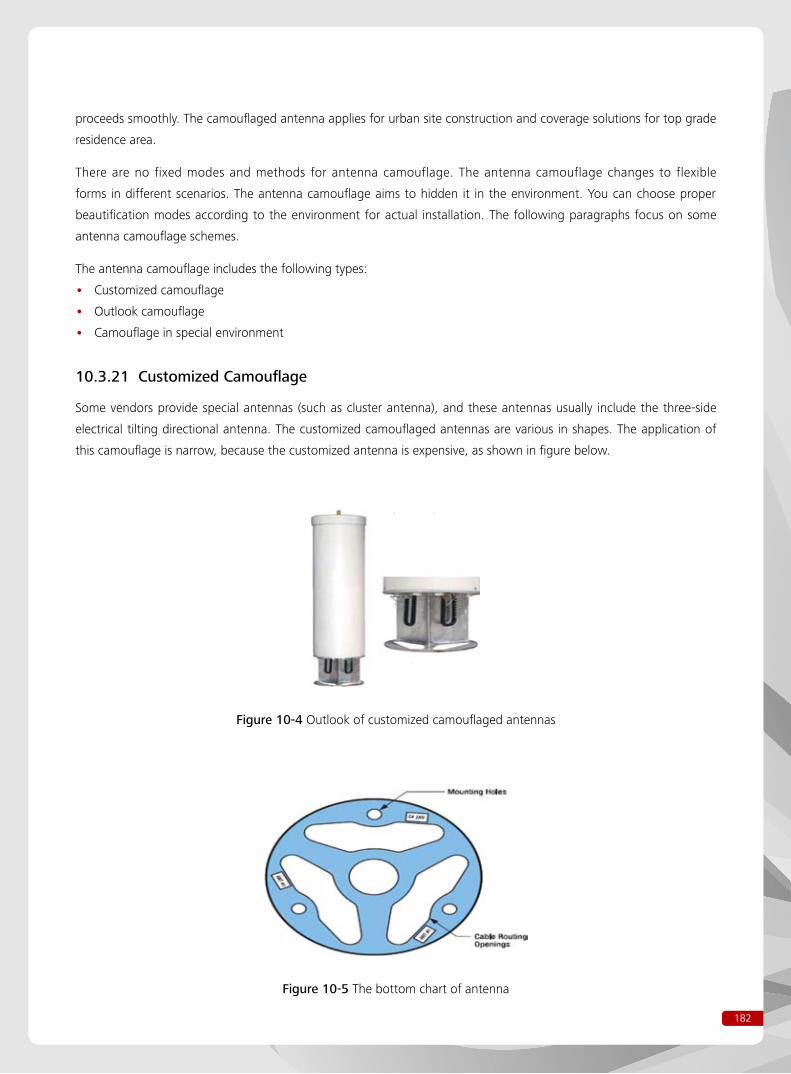
182
proceeds smoothly. The camouflaged antenna applies for urban site construction and coverage solutions for top grade
residence area.
There are no fixed modes and methods for antenna camouflage. The antenna camouflage changes to flexible
forms in different scenarios. The antenna camouflage aims to hidden it in the environment. You can choose proper
beautification modes according to the environment for actual installation. The following paragraphs focus on some
antenna camouflage schemes.
The antenna camouflage includes the following types:
Customized camouflage •
Outlook camouflage •
Camouflage in special environment •
10.3.21 Customized Camouflage
Some vendors provide special antennas (such as cluster antenna), and these antennas usually include the three-side
electrical tilting directional antenna. The customized camouflaged antennas are various in shapes. The application of
this camouflage is narrow, because the customized antenna is expensive, as shown in figure below.
Figure 10-4 Outlook of customized camouflaged antennas
Figure 10-5 The bottom chart of antenna
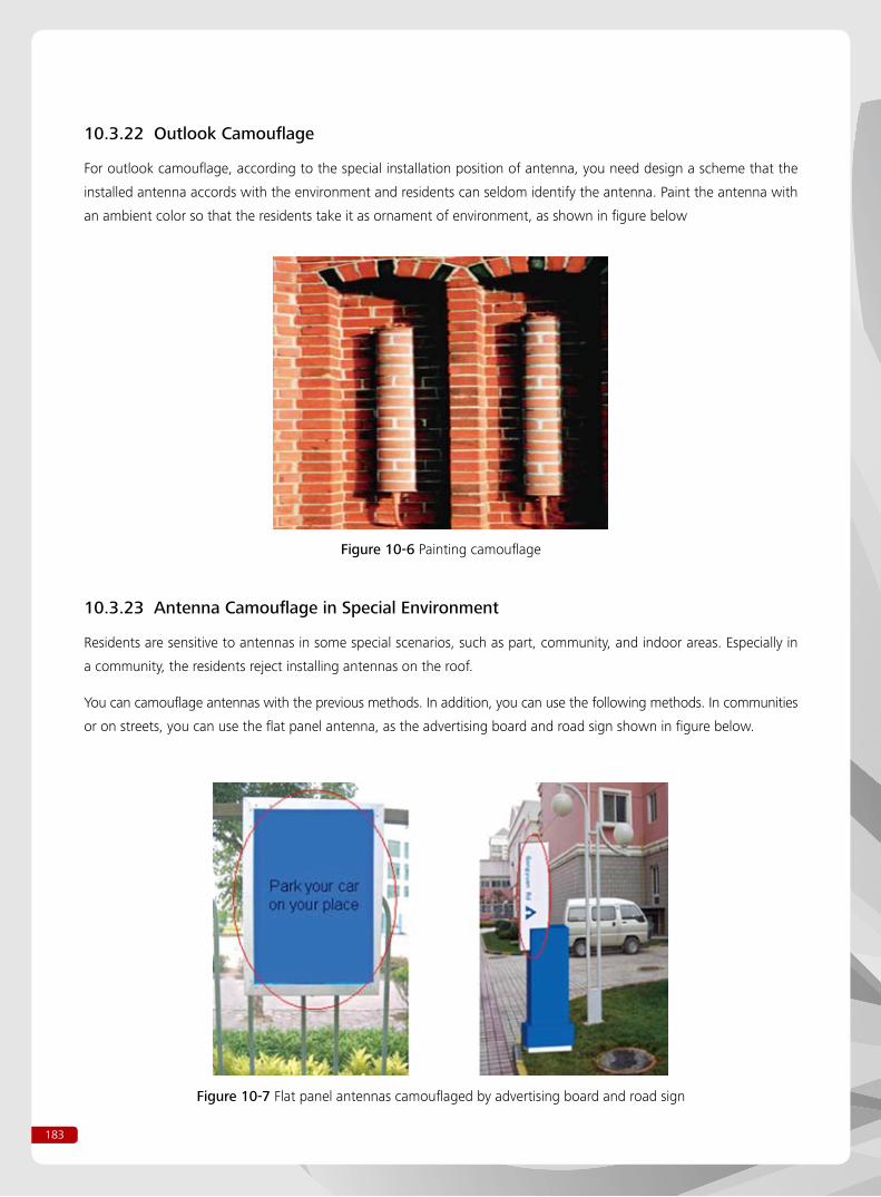
183
10.3.22 Outlook Camouflage
For outlook camouflage, according to the special installation position of antenna, you need design a scheme that the
installed antenna accords with the environment and residents can seldom identify the antenna. Paint the antenna with
an ambient color so that the residents take it as ornament of environment, as shown in figure below
Figure 10-6 Painting camouflage
Figure 10-7 Flat panel antennas camouflaged by advertising board and road sign
10.3.23 Antenna Camouflage in Special Environment
Residents are sensitive to antennas in some special scenarios, such as part, community, and indoor areas. Especially in
a community, the residents reject installing antennas on the roof.
You can camouflage antennas with the previous methods. In addition, you can use the following methods. In communities
or on streets, you can use the flat panel antenna, as the advertising board and road sign shown in figure below.
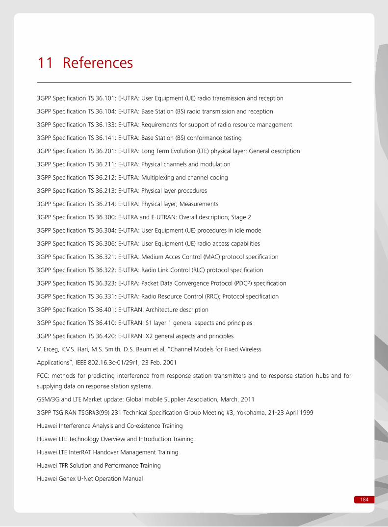
184
11 References
3GPP Specification TS 36.101: E-UTRA: User Equipment (UE) radio transmission and reception
3GPP Specification TS 36.104: E-UTRA: Base Station (BS) radio transmission and reception
3GPP Specification TS 36.133: E-UTRA: Requirements for support of radio resource management
3GPP Specification TS 36.141: E-UTRA: Base Station (BS) conformance testing
3GPP Specification TS 36.201: E-UTRA: Long Term Evolution (LTE) physical layer; General description
3GPP Specification TS 36.211: E-UTRA: Physical channels and modulation
3GPP Specification TS 36.212: E-UTRA: Multiplexing and channel coding
3GPP Specification TS 36.213: E-UTRA: Physical layer procedures
3GPP Specification TS 36.214: E-UTRA: Physical layer; Measurements
3GPP Specification TS 36.300: E-UTRA and E-UTRAN: Overall description; Stage 2
3GPP Specification TS 36.304: E-UTRA: User Equipment (UE) procedures in idle mode
3GPP Specification TS 36.306: E-UTRA: User Equipment (UE) radio access capabilities
3GPP Specification TS 36.321: E-UTRA: Medium Acces Control (MAC) protocol specification
3GPP Specification TS 36.322: E-UTRA: Radio Link Control (RLC) protocol specification
3GPP Specification TS 36.323: E-UTRA: Packet Data Convergence Protocol (PDCP) specification
3GPP Specification TS 36.331: E-UTRA: Radio Resource Control (RRC); Protocol specification
3GPP Specification TS 36.401: E-UTRAN: Architecture description
3GPP Specification TS 36.410: E-UTRAN: S1 layer 1 general aspects and principles
3GPP Specification TS 36.420: E-UTRAN: X2 general aspects and principles
V. Erceg, K.V.S. Hari, M.S. Smith, D.S. Baum et al, “Channel Models for Fixed Wireless
Applications”, IEEE 802.16.3c-01/29r1, 23 Feb. 2001
FCC: methods for predicting interference from response station transmitters and to response station hubs and for
supplying data on response station systems.
GSM/3G and LTE Market update: Global mobile Supplier Association, March, 2011
3GPP TSG RAN TSGR#3(99) 231 Technical Specification Group Meeting #3, Yokohama, 21-23 April 1999
Huawei Interference Analysis and Co-existence Training
Huawei LTE Technology Overview and Introduction Training
Huawei LTE InterRAT Handover Management Training
Huawei TFR Solution and Performance Training
Huawei Genex U-Net Operation Manual

Copyright © Huawei Technologies Co., Ltd. 2011. All rights reserved.
No part of this document may be reproduced or transmitted in any form or by any means without prior written consent of Huawei Technologies Co., Ltd.
General Disclaimer
The information in this document may contain predictive statements including,
without limitation, statements regarding the future financial and operating results,
future product portfolio, new technology, etc. There are a number of factors
that could cause actual results and developments to differ materially from those
expressed or implied in the predictive statements. Therefore, such information
is provided for reference purpose only and constitutes neither an offer nor an
acceptance. Huawei may change the information at any time without notice.
HUAWEI TECHNOLOGIES CO., LTD.
Huawei Industrial Base
Bantian Longgang
Shenzhen 518129, P.R. China
Tel: +86-755-28780808
Version No.: M3-121210199-20110718-C-1.0
www.huawei.com
Trademark Notice
, HUAWEI, and are trademarks or registered trademarks of Huawei Technologies Co., Ltd.
Other trademarks, product, service and company names mentioned are the property of their respective owners.
Consultant:
Wang Tao
Editors-in-chief:
Liu Jinghai, Cheng Tangbai, Yang Bo
Editors:
Lin Guangpu, Dong Fei, Zhong Fanliang, Xu Haihong,
Jin Keyou, Xie Guozhu, Li Guoyue, Gao Zhengwei,
Zhao Yinghe, Zhang Fan, Hao Guangming, Zhou Dongfei,
Ma Guotian, Hu Kangyan, Chen Qi, Wang Mingmin,
Zhou Zhibing, Zhao Xinlei, Liu Yingwei, Fang Minxi,
Liu Yadong, Fang Minghai, Xiang Rui
Auditors:
Lin Guangpu, Dong Fei, Ying Weimin, He Gang, Tan Zhu


![Huawei eWBB LTE Solution[1]](https://img.pdfslide.us/doc/110x75/55cf9ac5550346d033a350a0/huawei-ewbb-lte-solution1.jpg)